Student achievement and birthday effects *

Bjarne Strøm

Department of Economics

Norwegian University of Science and Technology

Dragvoll

N-7491 Trondheim

Norway

Abstract

The paper explores the strict school enrolment rules to estimate the effect of age at school

entry on school achievement for 15-16 year old students in Norway using achievement tests in

reading from OECD-PISA. Since enrolment date is common and compulsory for all students

born in a particular calendar year, it is possible to identify the pure effect of enrolment age

holding the length of schooling constant. The results indicate that the youngest children (born

in December) face a significant disadvantage in reading compared to their older classmates.

These results suggest that more flexible enrolment rules should be considered to equalize the

opportunities of the children.

JEL codes:I21, I28, J34

Keywords: Enrolment age, student test scores

Paper prepared for presentation at the CESifo-Harvard University/PEPG Conference on

“Schooling and Human Capital in the Global Economy: Revisiting the Equity-Efficiency

Quandary,” CESifo Conference Center, Munich, September 3-4, 2004. Present version, July

2004.

* Comments from Hans Bonesrønning, Torberg Falch, Oddbjørn Raaum and participants at

the 2004 Annual Meeting of Norwegian Economists, Trondheim are gratefully acknowledged.

1

1. Introduction

While several studies show that student characteristics and family background are important

factors shaping students performance in school, economists have paid little attention to the

relationship between educational outcomes and the age at which students are enrolled in

schools. Cognitive theories give ambiguous predictions on this issue. On the one hand, some

theories suggest that young children are more receptive for learning than older ones, while

other theories takes the position that children have to reach a certain age in order to learn

more complex material [Mayer and Knutson (1999)]. This suggests that the relationship

between student achievement and age at enrolment depends on the curriculum faced by the

children when they are exposed to schooling. Further, the effect of enrolment age can be

highly non-linear, i.e. children may benefit from starting at age 7 compared to age 8, while

they may lose from starting at age 5 compared to age 6. Finally, although enrolment age may

be important for the child’s learning in the first grades, the effects may fade as the children

become older. Ultimately, the relationship between achievement and school enrolment age is

an empirical one that deserves attention.

The issue is important when policymakers make decisions on school entry rules, i.e. whether

children should start school at age 5, 6 or 7. Further, the degree of flexibility in the school

entry rules is a policy question. On the one hand, low cost is an argument for inflexible rules.

A rule saying that all children born in a calendar year shall enter school at the same time is

easy to run and implies small administrative costs compared to a system where the parents

have some choice of the school enrolment time, potentially combined with individual testing

procedures. On the other hand, if there is a relationship between children’s age and the ability

to learn, strict rules may hurt children born in specific parts of the year. Thus, if reform

towards more enrolment flexibility is to be considered such negative effects from strict rules

should be identified and quantified. This paper addresses the question whether students gain

or lose by being exposed to schooling at a younger age than their classmates, holding the

quantity of schooling constant.

Empirical studies have not yet produced clear evidence on the issue. Some studies by

specialists in pedagogy and psychology find that the youngest children in a grade seem to

perform less well than their older classmates in several dimensions; lower test scores, higher

1

2

propensity to repeat a grade and more likely to qualify for special education1. Others find that

younger children do equally well as their younger class mates. A recent study by Mayer and

Knutson (1999) from the US, using more sophisticated statistical methods, suggest that the

younger students have even higher test scores than their older classmates controlling for

schooling quantity. Most of these studies investigate the effects in the first grades. A

particular issue in this paper is to study the age effect on achievement when students are about

to leave compulsory schooling, since this achievement is likely to directly affect their future

career in the labour and education market.

While most of the studies are done by none-economists, two economic papers have studied

the link between age at enrolment and performance in the education and labour market. First,

Leuven et al. (2003) use variation in potential enrolment age together with the incidence of

holidays to estimate the effect of potential time in school on achievement for young Dutch

children. Variation of birthdays relative to the summer holiday introduces an exogenous

variation in potential time in school. They find that conditional on age, potential time in

school increases achievement only for disadvantaged students. Their findings imply that the

age effect and time in school effect cancel out for non-disadvantaged students.

Second, Angrist and Krueger (1991) used quarter of birth as an instrument for length of

schooling in human capital earnings equations. Since US compulsory school laws imply that

students have to remain in school until their 16.th or 17.th birthday (varies across states) and

the school year starts in the third quarter, students born early in the year will have more

schooling than students born in the third quarter. The identifying assumption is that quarter of

birth does not affect earnings or productivity directly, only through the variation in length of

schooling. Thus, an investigation of possible direct effects of age at enrolment on student

performance is worthwhile in order to evaluate the general validity of the Angrist and Krueger

approach.

An important challenge when addressing the age effect empirically is to isolate the effect of

enrolment age from the effect of schooling quantity. This problem arises if children exposed

to schooling at a young age also receive more schooling (measured as months of schooling)

than children enrolled at an older age. Another, and related challenge is the possibility that

1 A brief survey can be found in Mayer and Knutson (1999).

2

3

some parents may choose the enrolment date strategically in order to optimise their child’s

opportunities. For instance, if children are required to start school no later than the year they

turn 7 years old, but parents are allowed to enrol their child earlier from the year they turn 6,

the age distribution within a grade will partly reflect the decision of parents to enrol their

child earlier or later. Thus, if school motivated parents have a higher propensity to delay

school entry for children born late in the year, a simple regression of individual test scores in

a given grade on student age measured in months could easily generate a biased estimate of

the age effect.

The present paper contributes to the existing literature on school entry age effects by

exploring the strict enrolment rules in Norway to identify and estimate the effect of age on

achievement for 15-16 year old students tested in 2000 in connection with the OECD-PISA

2000 program. Norwegian children are exposed to very strict enrolment rules as the school

law requires every child born in a certain calendar year to start school at the same point in

time. An important element in the education policy in Norway has been to integrate children

with different backgrounds and ability. Most important for the question at hand is that the

possibility to except from the school entry rule by starting earlier or later is severely limited.

As argued below, in practise, very few students get exception from the rules. Further, students

almost never retain a grade or get promoted faster than the normal rule. Thus, a grade consists

of children born in the same calendar year, with the students born in January nearly one year

older than their youngest classmates. The basic identification assumption is that the strict

enrolment rules and the absence of grade repetition allow me to treat the variation in birth

dates across students in a given grade as exogenous. By estimating reduced form education

production functions extended by students’ age, I find that 15-16 year old students born late in

the calendar year achieve significantly lower test scores in reading compared to their oldest

classmates. This result is quite robust across several econometric specifications including

fixed school effects and different sub-samples.

The paper is organized as follows: Section 2 presents a simple model to discuss enrolment age

effects. Section 3 summarizes the existing literature on age effects. Section 4 describes the

institutional details and the identification strategy. Section 5 presents the data and empirical

results, while section 6 concludes.

3

4

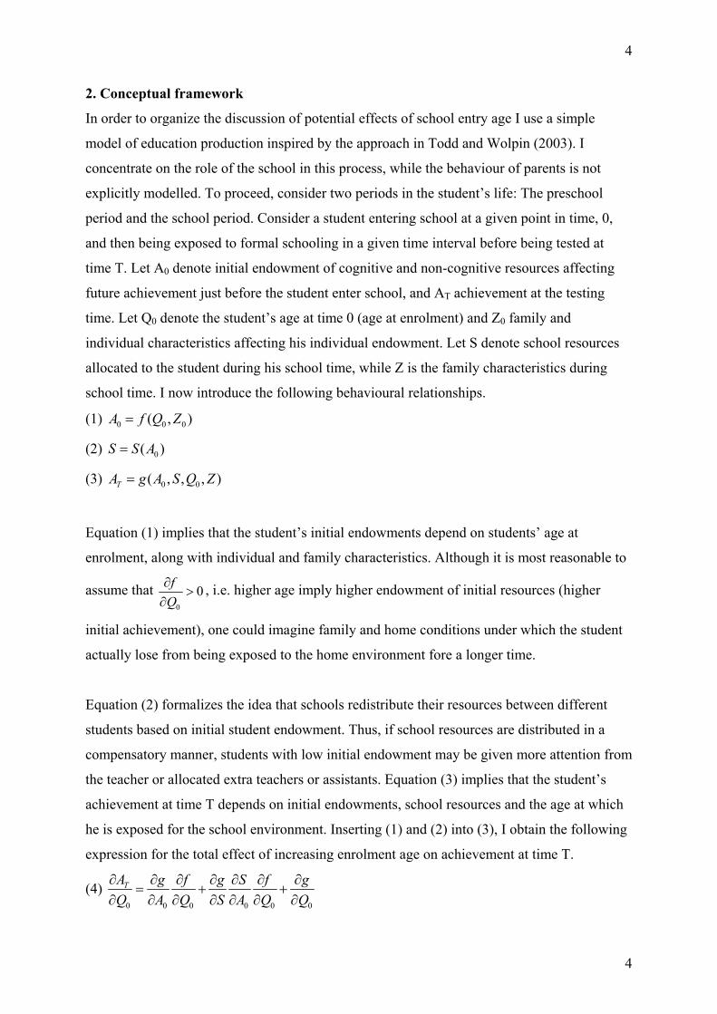
2. Conceptual framework

In order to organize the discussion of potential effects of school entry age I use a simple

model of education production inspired by the approach in Todd and Wolpin (2003). I

concentrate on the role of the school in this process, while the behaviour of parents is not

explicitly modelled. To proceed, consider two periods in the student’s life: The preschool

period and the school period. Consider a student entering school at a given point in time, 0,

and then being exposed to formal schooling in a given time interval before being tested at

time T. Let A0 denote initial endowment of cognitive and non-cognitive resources affecting

future achievement just before the student enter school, and AT achievement at the testing

time. Let Q0 denote the student’s age at time 0 (age at enrolment) and Z0 family and

individual characteristics affecting his individual endowment. Let S denote school resources

allocated to the student during his school time, while Z is the family characteristics during

school time. I now introduce the following behavioural relationships.

(1) 0 0( , )A f Q Z= 0

(2) 0( )S S A=

(3) 0 0( , , , )TA g A S Q Z=

Equation (1) implies that the student’s initial endowments depend on students’ age at

enrolment, along with individual and family characteristics. Although it is most reasonable to

assume that 0

0fQ∂

>∂

, i.e. higher age imply higher endowment of initial resources (higher

initial achievement), one could imagine family and home conditions under which the student

actually lose from being exposed to the home environment fore a longer time.

Equation (2) formalizes the idea that schools redistribute their resources between different

students based on initial student endowment. Thus, if school resources are distributed in a

compensatory manner, students with low initial endowment may be given more attention from

the teacher or allocated extra teachers or assistants. Equation (3) implies that the student’s

achievement at time T depends on initial endowments, school resources and the age at which

he is exposed for the school environment. Inserting (1) and (2) into (3), I obtain the following

expression for the total effect of increasing enrolment age on achievement at time T.

(4) 0 0 0 0 0

TA g f g S f gQ A Q S A Q Q∂ ∂ ∂ ∂ ∂ ∂ ∂

= + +∂ ∂ ∂ ∂ ∂ ∂ ∂ 0

4

5

According to (4) the total effect of age at enrolment on achievement operates through three

main channels. The first term in (4) reflects that an increase in enrolment age affects initial

endowments. Since the achievement effect of higher endowment is positive and initial

endowment is positively related to age at enrolment, the first term is positive. It is reasonable

to believe that the effect of age at enrolment through this effect is most pronounced in the first

grades, i.e. for low T. The second term represents the effect of enrolment age on the

distribution of school resources. If school resources are distributed across students in a

compensatory manner, this term is negative. The last term represents the direct effect on

achievement from being exposed for formal schooling at an older age. To illustrate, if a

teacher reads the same text to two otherwise equal students, one exactly 9 years old and the

other nearly 8 years old, the effect on achievement for the two students may differ. Some

cognitive theories suggest that young children are more receptive for learning than older ones,

while others take the position that children have to reach a certain age in order to learn more

complex material. Thus, the sign of the third effect is ambiguous and it would obviously

depend on the curriculum faced by the students.

The most satisfactory approach would be to identify the separate contribution from each of

these channels. However this is a very demanding task. For instance, identification of the pure

school learning effect (the third term in equation (4)), requires conditioning on initial

endowments immediately prior to school entry and on school resources allocated to individual

students during their whole school career. Since this requires unrealistic amounts of data, the

ambition in this paper is to estimate the total effect of exogenous variation in school entry age

on achievement, conditional on school quantity (measured in school years or months). This

question should be of interest to policymakers when deciding whether to change the

compulsory enrolment age or to make the enrolment rules more flexible. The empirical

challenge discussed below is to ensure that the school entry age variation is exogenous and

possible to separate from variation in length of schooling.

3. Existing literature.

The existing literature on education outcomes and school enrolment age is quite diverse.

Some educational studies have typically found that the oldest children in a cohort perform

5

6

better than their younger classmates, but that the effects are relatively small and tend to

decrease as the children reach higher grades [Crosser (1991), Sharp et. al. (1994)]. An

interesting study by Cahan and Cohen (1989) used data on achievement for 5 and 6-graders in

Jerusalem schools to estimate the separate impacts of one year of additional schooling and

one year of age on cognitive development. Their point of departure is that students born close

to the cut off enrolment date are approximately similar in age, but those born just before the

cut off date have one year additional schooling compared to those born just after the cut off

date. The achievement difference between these children then gives an estimate on the effect

of an additional year of schooling holding age constant. The age effect was estimated by

comparing within grade achievement between those born early and late in the academic year.

A problem in their study is that school admission was delayed or accelerated compared to the

normal cut off date for a significant part of the children and this was most frequent for

children born close to the cut off date. To cope with this problem, they excluded from the

within grade analysis the children who were under-aged or over-aged and those born close to

the cut off date. While they estimate a positive effect of age on within grade achievement,

they conclude that one year of additional schooling gives three times more achievement than

one year of age.

Morrison et al. (1997) tried to isolate the pure school learning age effect from the initial

endowment effects. They used cut off school entry age to compare the achievement growth of

first grade children born just after the cut off date with the achievement growth of children

born just before the cut off date. In addition, to obtain a pre-post research design, they used

kindergarten children just too young to join the first grade as a control group to assess how

much a child at the same age would have learnt when not being in first grade. They used a

total sample of 539 children from 26 schools in one city in Canada. The results showed that

the youngest and oldest children in first grade had similar growth in achievement and that the

youngest first graders did significantly better than the control group. Thus, they argue that

early enrolment will likely have a positive effect on student performance in early grades.

However, their results do not provide evidence on the long time effect from early schooling.

Another interesting recent study by Mayer and Knutson (1999) extends the literature on

achievement effects by using data from US schools and exploring differences in enrolment

age and procedures across states to obtain identification of the causal effect of age. Their

results show that children exposed for schooling at a younger age scores higher on cognitive

6

7

tests compared to older ones conditional on schooling length. This latter result may suggest

that lower school enrolment age is a promising policy tool.

Other researchers have investigated the effect of school entry age on other aspects of student

behaviour. Shephard and Smith (1986) found that children who were young relative to their

classmates, i.e. born just before the school entry cut-off date, had a higher risk of grade

repetition. Another strand of literature studies the relationship between age in school and the

incidence of psychological disorders. Based on a large sample of children from UK, Goodman

et. al. (2003) presents evidence that the youngest children in a school year is more prevalent

to psychological disadvantage than older children

An important drawback of many of the studies of the age effect on several aspects of student

performance is that they do not take into account that the possibility of strategic enrolment

decisions by the parents along with grade repetition decisions made the schools may cause

serious bias in the estimated effects. Another weakness of many studies is the usually small

samples used by the researchers.

As to research done by economists, a recent interesting paper by Leuven et al. investigate the

relationship between early test scores and time in school using exogenous variation in the

potential schooling time generated by enrolment rules in the Dutch school system. Dutch

children are required to start school at the beginning of the school year they turn 5 years old2.

However, the children may actually start school from their 4.th birthday on. The children

choosing this option, spends the time in the first grade, and than starts grade one again from

the beginning of the school year. Children having their 4.th birthday before the summer

holiday has a lower number of potential school months than children having their 4.birthday

after the holiday, conditional on age. This creates an exogenous variation in potential school

time conditional on age, and the authors find that increased potential school time increase

second grade test scores for the disadvantaged students only. On the one hand, starting school

earlier increases school length, which has a positive effect on test scores. On the other hand,

being exposed for schooling at a younger age has a negative effect on achievement. Their

findings indicate that the net effect on achievement is positive only for disadvantaged

2 The school year in the Netherlands lasts from October 1 to September 30.

7

8

students. It is however an open question to which extent these results carry over to

achievement in higher grades.

Another type of research, initiated by Angrist and Krueger (1991), have used birth quarter as

an instrument for education attainment in human capital earnings equations. Since US

students in the time period analysed were obliged to stay in school until a certain age that

varied across states, students born in different quarters of the year would have different

compulsory length of schooling. Interestingly, the identification assumption behind the

Angrist and Krueger study was that age at enrolment did not affect worker productivity

directly; only indirectly through the length of compulsory schooling. This assumption would

not be valid if enrolment age affects student achievement for given quantity of schooling, a

question raised by Bound and Jaeger (2000) in their critic of the Angrist and Krueger

approach.

To sum up, although researchers from several disciplines have investigated the relationship

between age at school entry and school and labour market performance, the evidence is so far

not conclusive. One particular problem with much existing research on the issue is the failure

to identify the total school entry age effect conditional on school quantity, particular in

circumstances when school entry age is to some extent a choice variable for the parents. A

second weakness is that most of the evidence is based on children in early grades. Thus the

size of the age effects on student’s achievement at the end of compulsory school is still an

open question.

4. Institutions, empirical strategy and data.

4.1. Institutional context and empirical strategy.

The empirical challenge is to estimate the effect of exogenous variation in students’ age on

student achievement conditional on school length. Most countries use specific cut off dates

such that children born within a certain time interval, i.e. a calendar year, starts school at the

same time. A simple strategy to identify age effects would then be to compare achievement

for children born at different dates in the calendar year using the assumption that birth dates

are randomly distributed within the year. At least two main obstacles may exist to this simple

procedure. First, many countries give parents some choice regarding enrolment date. As an

illustration, in the Netherlands, all children is required to enrol in the beginning of the

academic year they turn five years old, but they have the option to enrol from their 4. birthday

8

9

[Leuven et. al. (2003)]. Second, in many countries students’ advancement from one grade to

another is conditional on a minimum achievement level. Both these possibilities will imply

that the age variation within a grade is not exogenous and that the length of schooling across

students within a grade is not constant. Thus, variation in achievement levels across student

ages within a grade would then reflect both variations in age, variations in school length and

potential variations in parents’ propensity to delay or accelerate school start for their children.

I will argue that three features of the schooling system in Norway make it possible to rely on a

simple empirical strategy to identify the age effect. First, the school enrolment date or year is

not subject to parental choice. According to the school law the students in the sample had to

enrol in school in the year they became 7 years old and had to join compulsory school for 9

years.3 Exemptions from this rule required a formal application from the parents, and the

application had to be approved by health and school specialists, while the final decision were

taken by the local government. Accordingly, very few children were exempted from the rule.

Second, while grade retention is quite normal in the US and several other countries around the

world, this almost never happen within the Norwegian compulsory school system. This is

consistent with the strong integration and equalizing policy that all students within a cohort

should be treated equal, and be given education in their ordinary classes. Thus, all students

who have been exposed to the Norwegian school system during their whole school career

have identical length of schooling. Third, private schools cover a negligible fraction of the

students, implying that the only realistic choice for the parents is the public school system

regulated by the school law. The public schools use a national curriculum and are subject to

national rules on maximum class sizes, criteria for special education and teacher certification.

Finally, all students start school in mid August and the school year lasts until mid June.

These institutional features imply that the enrolment date for the children born in a certain

calendar year is in reality not a choice variable for the parents, and that nearly all students

tested in a given grade have been exposed for exactly the same number of school years and

months. Further, as the cut-off date is January 1, a student born in January entered school

nearly 1 year older than a student born in December. The institutional setting described above

suggests that the age variation within a grade is only due to differences in birth date. To

ensure that we only include students exposed to the Norwegian public school system

3 From 1997, the school entry age was changed to 6 years, while the number of school years increased from 9 to 10.

9

10

throughout their whole school career, we include only students born in Norway. The fact that

99.5% of the remaining students in public schools born in 1984 in the Norwegian PISA study

reported that they were in grade 10 documents that the institutional arrangements regarding

enrolment and grade were actually enforced. Thus, the Norwegian setting provides a nice

opportunity to identify effects from age at school entry on student performance. The simplest

way to do this is to compare average test scores for students born in different quarters within a

year. However, this will not be a satisfactory strategy if birth season differs systematically

between individuals with different backgrounds. For instance, if highly educated parents for

some reason have a higher propensity to have children born in the first quarter of the year than

others, simply comparing average test scores could erroneously indicate that children born

early in the year have higher test scores. Accordingly, I choose to embed the analysis of age

of enrolment effects in the education production function tradition, see Hanushek (2003) and

Todd and Wolpin (2003) for an extensive review. This literature emphasizes the role of both

individual background variables and school resource variables as the main determinants of

education achievement.

4.2. Data description

Empirical research on enrolment age effects on student achievement requires access to

achievement data combined with detailed information on student age and grade. The data

used in this paper consists of the Norwegian part of the international PISA 2000 data from

testing 15-16 year olds in reading, which in addition to test scores includes of a huge amount

of information on individual background factors including birth month and year. The tests

were completed between March 27 and April 15, 2000. Since I only have information on test

scores at one point in time, the test scores reflect the cumulative effect of school, individual

and family effects during the entire life and school time up to the test date. The reading test

consisted of three parts: One part focused on retrieving information, another part focused on

interpreting text and the third part focused on reflection and evaluation. Within each of these

parts, the students answered several questions. To obtain a reading test score index, the PISA

study used Item Response Theory (IRT) to calculate weighted averages of the correct answers

to all questions with the difficulty of the questions as weights4. In a final step the individual

test scores were standardized across OECD countries with mean 500 and standard error equal

4 More details on this procedure can be found on the PISA web site, http://www.pisa.oecd.org/index.htm. Fertig and Smith (2002), Wolter and Vellacott (2002) and Fertig (2003) are recent examples on studies using the PISA data to estimate education production functions.

10

11

to 100. The methodology used to obtain the test scores in the PISA study is very similar to

that used in the international study of student performance in mathematics and science

(TIMMS)5.

To ensure that the students included in the analysis have all been exposed to the Norwegian

school system in their whole school career, I exclude students born in other countries.

Moreover, I exclude from the analysis the few students reporting grades other than grade 10

and students in non-public schools.

5. Empirical results.

5.1. Descriptive evidence

I first present in Table 1 the raw mean test scores for students born in different quarters of the

year 1984. The picture is quite clear: Students born in the first quarter have a mean score

about 17 points above those born in the fourth quarter. This is a first indication that the

youngest students face a real disadvantage relative to their older classmates. Figure 1 presents

a further illustration of the relationship between test scores and age with birth month on the

horizontal axes and mean test score on the vertical axes. Measuring birth date at the monthly

frequency reveals much the same broad picture: older students have a higher test score than

younger ones. However, such raw data differences can be driven by composition effects due

to systematic relationships between birth season and family background variables affecting

student achievement. Thus, it is important to control for other family and school specific

factors that may affect student performance. Another reason for estimating the age effect

conditional on other factors determining achievement is to gauge the quantitative effect of age

variation.

5.2. Reduced form education production functions.

In this section I present the results from estimation of reduced form education production

functions extended by variables representing student age. While the PISA data set contains

numerous variables describing the students attitudes towards school, homework, time use and

so on, these variables are likely to be outcome variables and thus should not be included as

determinants of achievement. One possible threat to my empirical strategy is the possibility

that birth season is correlated with observable or unobservable determinants of student

5 Woessmann (2003) contains a detailed discussion of the TIMMS data. Hanushek and Luque (2002) is another recent example of the use of these data in estimation of education production functions.

11

12

performance. Consequently, I choose to include reasonably objective student background and

family variables traditionally used in education production functions: Gender, father and

mother’s education and labour market attachment, and educational resources at home are

standard variables. Following this tradition I include a gender dummy variable, dummy

variables indicating whether mother (father) has higher education and dummy variables

indicating whether mother (father) has a fulltime job. To account for educational resources at

home I include dummy variables indicating whether the family has between 10 and 50 books,

between 50 and 100 books, between 100 and 250 books and above 250 books at home.

Families with less than 10 books serve as the reference group.

Further, a number of studies including Behrman and Taubman (1986), Plug and Wijverberg

(2003), Wolter and Vellacot (2002) and Bonesrønning (2003) find that birth order and family

size have significant effects on student achievement. Older siblings are found to achieve

higher test scores and to have a higher propensity to attain college, than younger ones

presumably because the oldest siblings and the children in small families receive more

education resources at home. If birth season tends to differ systematically between say the

first and second child, it would be important to control for these variables, and accordingly I

include the students number of siblings and dummy variables indicating whether the student is

single child, first born and middle born with youngest child being the reference category.

Moreover, I also include a variable indicating whether the student speaks another language

than Norwegian. This is a potential important variable in determining reading test scores. A

final variable included to capture family background is a dummy variable indicating whether

the student lives with both parents.

Another determinant of student performance is school resources. Since the coefficient of

interest is an individual characteristic, we can control for resources affecting all students in

the school equally in a very general way by including school specific effects. This is

potentially important if birth season vary geographically.

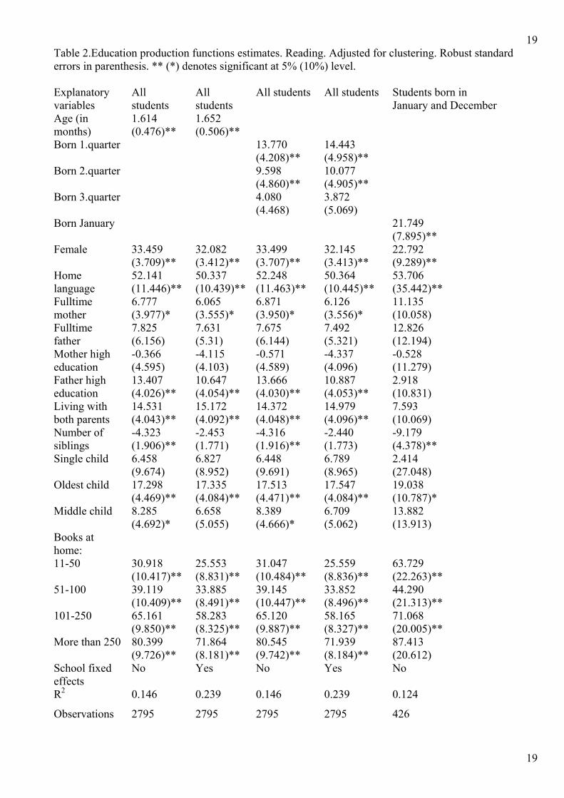
The first column in Table 2 shows the result from a simple specification with the student age

measured in months and with only student and family characteristics included. The effect of

student age is significantly positive and implies that a student born in January scores about 17

points higher than a student born in December, close to the gap found in the raw data. The

second column in Table 2 extends the specification with school fixed effects and the results

12

13

are almost unchanged. To account for possible non-linearities in the age effect, the third and

fourth columns report the results from specifications with birth quarters. Again, the picture is

remarkably stable, and implies that a student born in the first quarter scores about 14 points

above students born in the fourth quarter of 1984. To gauge the quantitative relevance of the

effect I compare the age effect with other standard determinants of student achievement. First,

the effect of being born in the first quarter of the year is approximately similar in magnitude

to the effect of having a father with high education. Second, the magnitude of the effect is

close to half of the gender achievement gap since girls are found to have a reading score about

30 points higher than boys. Thus, based on these findings it is tempting to conclude that the

rigid enrolment rules in Norway implies that students born late in the year face a significant

disadvantage compared to their older classmates.

So far I have shown that the conclusion is robust with respect to the inclusion of several

observed family characteristics and observed and unobserved school variables. It is still a

possibility that part of the effect may be driven by unobserved family characteristics. If some

potential parents believe in a negative effect on student performance from starting school at a

young age, they may manipulate the time of birth in order to optimise their child’s age at

school enrolment. In particular, if unmeasured parental variables determining the propensity

to fine-tune birth time with respect to school enrolment age is positively correlated with

student performance, the above estimates may be biased upwards. However, the extent to

which birth-date can be fine tuned is physically limited. One strategy to account for this

would be to restrict the sample to only include students born very close to the cut-off date.

Ideally, if I could include only students born, say the last week of December and those born

the first week of January, being the youngest or oldest in class is reasonably a random event.

Unfortunately, I cannot get that far since I only have data on birth month. Even if exact birth

date data were available, reliable results from such a strategy would probably require a much

larger total sample of students tested in each country than in the PISA study. A second best

alternative is to restrict the sample to only those born in January and December and include a

dummy variable indicating whether the student is born in January. The results from this

specification are shown in the fifth column of Table 2. While the sample is quite small (425

students), the model reveals a numerically higher effect of student age than the above

specification. According to the results from this restricted sample, a student born in January

have close to 22 points higher reading score than a student born in December, other factors

constant. Although, this strategy is less than perfect in removing non-randomness in student

13

14

birth dates, it supports the earlier results that the youngest students face an important

disadvantage due to the strict enrolment system.

5.3. Sub-sample results

Having shown that variation of student age within a grade, conditional on schooling quantity

is generally important, it is of interest to investigate whether the effect differs between student

groups. For instance, if the physical and mental development of boys are generally slower

than for girls, being born late in the year may be more negative for boys than for girls. The

two first columns in Table 3 show the estimation results when the sample is split between

male and female students. The effect of student age (in months) is much the same across

genders, while the effect of other family and personal characteristics differs quite substantial.

Another question is that the effect of being exposed to schooling at an earlier age may differ

between students with different home resources. One possibility is that children with small

educational resources at home in the preschool period may actually gain from being exposed

to school at a young age. The results in Leuven et al. (2003) seem to indicate that the net

effect on early test scores from more potential school time is positive for children with low

parental resources. Unfortunately, I only have information on home resources at the test date,

and thus cannot isolate the effect of home resources during the preschool period from the

effect of home resources during the whole school career. Nevertheless, to provide some

evidence on the distributional effects, I estimate the model on the sample of students with and

without higher education. The results from this exercise are presented in the third and fourth

columns in Table 3. There is some evidence that the age effect is stronger for students with

high educated parents than for students with parents without higher education, but the

difference is not dramatic. The same pattern arise if I split the sample according to the number

of books at home as shown in the fifth and sixth columns in Table 3 where the model is

estimated on the sample of students reporting less than 100 books at home and another sample

of students reporting having more than 250 books at home. Thus, it is tempting to conclude

that there is some weak evidence that the disadvantage from being born late in the calendar

year is highest for children with relatively large home and parental resources.

5. Conclusion

This paper has investigated the relationship between students’ achievement at the end of

compulsory school, and the age at which students are exposed to formal schooling, holding

14

15

schooling time constant. Using the Norwegian institutional arrangements with strict enrolment

rules the variation in enrolment age generated by birthday variation is reasonably exogenous.

The results show that younger students have a significant disadvantage relative to their older

classmates. I find that the oldest students, born in January just after the school entry cut off

date score nearly 1/5 of a standard deviation higher than the youngest students born in

December, just before the cut off date. This age effect is approximately equal to the estimated

effect from having father with high education. Further, I find that the age effects are fairly

similar across students with different family backgrounds, although some weak evidence

indicated that children with high educated parents suffered the most from being born late in

the calendar year. While I cannot offer a structural interpretation of the results, it does indicate

that there is a potential gain from using more flexible school entry rules.

15

16

References: Angrist, J. and A. Krueger (1991): Does compulsory school attendance affect schooling and earnings? Quarterly Journal of Economics 106 (4) 979-1014. Behrman, J.R. and P. Taubman (1986): Birth order, schooling and earnings. Journal of Labor Economics 4, 121-45. Bonesrønning, H. (2003): Birth order and student achievement: Is the relationship conditional upon mother’s education? Mimeo. Department of Economics, Norwegian University of Science and Technology. Bound, J. and D. A. Jaeger (2000): Do compulsory school attendance laws alone explain the association between quarter of birth and earnings? Worker Well-being 19, 83-108. Cahan, S. and N. Cohen (1989): Age versus schooling effects on intelligence. Child Development 60, 1239-1249. Crosser, S. (1991): Summer birth date children: Kindergarten entrance age and academic achievement. Journal of Educational Research 84, 140-46. Fertig, M. (2003): Educational production, endogenous peer group formation and class competition-Evidence from the PISA 2000 study. IZA Discussion Paper no. 714, IZA-Bonn. Fertig, M. and C. M. Smith (2002): The role of background factors for reading literacy: Straight national scores in the PISA 2000 study. IZA Discussion Paper no. 545, IZA-Bonn. Goodman, R., J. Gledhill and T. Ford (2003): Child psyciatric disorder and relative age within school year: cross sectional survey of large population sample. British Medical Journal 327 (August) 472-475. Hanushek, E. H. (2003): The failure of input-based schooling policies. Economic Journal 113, 64-98. Hanushek, E. H. and J. A. Luque (2003): Efficiency and equity in schools around the world. Economics of Education Review 20, 481-502. Leuven, E. M. Lindahl, H. Oosterbeek and D. Webbink (2003): The effect of potential time in school on early test scores. Unpublished. Department of Economics, University of Amsterdam. Mayer, S. E. and D. Knutson (1999): Does the timing of school affect how much children learn? In Mayer, S. E. and P. E. Peterson, editors, Earning and Learning: How School Matters, p. 70-102. Brookings Institution and Russell Sage Foundation. Morrison, F. J., E. G. Griffith and D. Alberts (1997): Nature-Nurture in the classroom: Entrance age, school readiness, and learning in children. Developmental Psychology 33, 254-262.

16

17

Plug, E. and W. Vijverberg (2003): Schooling, Family Background, and Adoption: Is It Nature or Is It Nurture? Journal of Political Economy 111, 611-641. Sharp, C., D. Hutchison and C. Whetton (1994). How do season of birth and length of schooling affect children’s attainment at key stage 1? Educational Research 36 (2), 107-21. Shephard, L. and M. Smith (1986): Escalating academic demand in kindergarten: Counterproductive policies. The Elementary School Journal 89, 135-145. Todd, P. E. and K. Wolpin (2003): On the specification and estimation of the production function for cognitive achievement. Economic Journal 113, 3-33. Wolter, S. and M. C. Vellacott (2002): Sibling Rivalry: A look at Switzerland with PISA data. IZA Discussion Paper no. 594, IZA-Bonn Woessmann, L. (2003): Schooling resources, educational institutions and student performance: the international evidence. Oxford Bulletin of Economics and Statistics 65, 117-170.

Table 1. Mean achievement across birth quarters. Students born 1984, 10.grade.

Birth quarter Mean test score

in reading

Number of students

1. Quarter 515.0 960

2. Quarter 512.4 1012

3. Quarter 504.2 893

4. Quarter 498.8 797

17

18

Figure 1. Average test score by birth month

480

485

490

495

500

505

510

515

520

525

1 2 3 4 5 6 7 8 9 10 11 12

month

Test

sco

re

18

19

19

Table 2.Education production functions estimates. Reading. Adjusted for clustering. Robust standard errors in parenthesis. ** (*) denotes significant at 5% (10%) level. Explanatory variables

All students

All students

All students All students Students born in January and December

Age (in months)

1.614 (0.476)**

1.652 (0.506)**

Born 1.quarter 13.770 (4.208)**

14.443 (4.958)**

Born 2.quarter 9.598 (4.860)**

10.077 (4.905)**

Born 3.quarter 4.080 (4.468)

3.872 (5.069)

Born January 21.749 (7.895)**

Female 33.459 (3.709)**

32.082 (3.412)**

33.499 (3.707)**

32.145 (3.413)**

22.792 (9.289)**

Home language

52.141 (11.446)**

50.337 (10.439)**

52.248 (11.463)**

50.364 (10.445)**

53.706 (35.442)**

Fulltime mother

6.777 (3.977)*

6.065 (3.555)*

6.871 (3.950)*

6.126 (3.556)*

11.135 (10.058)

Fulltime father

7.825 (6.156)

7.631 (5.31)

7.675 (6.144)

7.492 (5.321)

12.826 (12.194)

Mother high education

-0.366 (4.595)

-4.115 (4.103)

-0.571 (4.589)

-4.337 (4.096)

-0.528 (11.279)

Father high education

13.407 (4.026)**

10.647 (4.054)**

13.666 (4.030)**

10.887 (4.053)**

2.918 (10.831)

Living with both parents

14.531 (4.043)**

15.172 (4.092)**

14.372 (4.048)**

14.979 (4.096)**

7.593 (10.069)

Number of siblings

-4.323 (1.906)**

-2.453 (1.771)

-4.316 (1.916)**

-2.440 (1.773)

-9.179 (4.378)**

Single child 6.458 (9.674)

6.827 (8.952)

6.448 (9.691)

6.789 (8.965)

2.414 (27.048)

Oldest child 17.298 (4.469)**

17.335 (4.084)**

17.513 (4.471)**

17.547 (4.084)**

19.038 (10.787)*

Middle child 8.285 (4.692)*

6.658 (5.055)

8.389 (4.666)*

6.709 (5.062)

13.882 (13.913)

Books at home:

11-50 51-100 101-250 More than 250

30.918 (10.417)** 39.119 (10.409)** 65.161 (9.850)** 80.399 (9.726)**

25.553 (8.831)** 33.885 (8.491)** 58.283 (8.325)** 71.864 (8.181)**

31.047 (10.484)** 39.145 (10.447)** 65.120 (9.887)** 80.545 (9.742)**

25.559 (8.836)** 33.852 (8.496)** 58.165 (8.327)** 71.939 (8.184)**

63.729 (22.263)** 44.290 (21.313)** 71.068 (20.005)** 87.413 (20.612)

School fixed effects

No Yes No Yes No

R2 0.146 0.239 0.146 0.239 0.124

Observations 2795 2795 2795 2795 426

20

Table 3. Table 2.Education production functions estimates. Reading. Adjusted for clustering.

Robust standard errors in parenthesis. ** (*) denotes significant at 5% (10%) level.

Explanatory variables

Females Males Both parents high education

None of parents high education

More than 250 books at home

Less than 100 books At home

Age (in months)

1.710 (0.657)**

1.556 (0.778)**

2.022 (0.884)**

1.595 (0.617)**

1.961 (0.823)**

1.462 (0.841)*

Female 39.136 (6.383)**

32.320 (5.324)**

44.435 (5.608)**

25.850 (5.549)**

Home language

27.821 (12.906)**

72.085 (19.754)**

27.337 (18.215)**

82.558 (23.092)**

52.587 (21.704)**

49.403 (17.755)**

Fulltime mother

10.025 (4.672)**

3.105 (5.742)

9.362 (7.051)

2.592 (5.394)

0.624 (6.297)

9.813 (5.894)

Fulltime father

15.559 (6.136)**

-2.327 (9.919)

1.801 (13.339)

5.467 (6.883)

14.082 (10.923)

-6.813 (7.619)

Mother high education

5.339 (5.493)

-5.842 (6.612)

12.116 (5.992)**

-8.495 (7.525)

Father high education

8.541 (5.161)*

18.795 (6.045)**

15.647 (6.647)**

10.932 (6.982)

Living with both parents

13.688 (5.235)**

16.158 (6.241)

16.908 (7.723)**

14.872 (6.360)**

5.199 (6.075)

10.750 (6.193)*

Number of siblings

-2.143 (2.556)

-5.547 (2.839)**

-7.171 (3.942)*

-4.648 (2.665)

-2.960 (3.237)

-8.357 (2.697)**

Single child 14.234 (12.257)

1.967 (13.249)

11.586 (20.627)

-2.094 (12.856)

15.179 (18.295)

-28.384 (14.113)

Oldest child 19.017 (5.393)**

14.467 (6.015)**

11.714 (7.504)

22.028 (6.812)**

22.235 (6.505)**

11.549 (7.144)

Middle child 7.098 (6.601)

7.131 (6.286)

10.453 (9.176)

11.287 (6.873)*

9.221 (8.651)

6.759 (7.017)

Books at home:

11-50 15.457 (12.676)

43.141 (14.215)**

41.215 (25.532)**

26.659 (11.923)**

32.01 (10.261)**

51-100 29.999 (12.821)**

46.246 (15.243)**

73.925 (24.453)**

31.596 (11.327)**

40.979 (10.370)**

101-250 55.917 (12.821)**

73.248 (13.401)**

88.835 (22.747)**

57.035 (11.830)**

More than 250

78.675 (11.911)**

79.980 (13.668)**

116.313 (23.611)**

63.583 (11.391)**

School fixed effects

No No No No No No

R2 0.152 0.103 0.159 0.149 0.091 0.096

Observations 1400 1394 899 1225 1091 1032

20