structures of supercavitating multiphase flows

International Journal of Thermal Sciences 47 (2008) 1263–1275www.elsevier.com/locate/ijts

Structures of supercavitating multiphase flows

Xiangbin Li a, Guoyu Wang a,∗, Mindi Zhang a, Wei Shyy b

a Department of Thermal Energy Engineering, Beijing Institute of Technology, Beijing 100081, People’s Republic of Chinab Department of Aerospace Engineering, University of Michigan, Ann Arbor, MI 48109, USA

Received 15 August 2007; received in revised form 24 November 2007; accepted 24 November 2007

Available online 8 January 2008

Abstract

Supercavitation around a hydrofoil is studied based on flow visualization and detailed velocity measurement. The main purpose of this study isto offer information for validating computational models, and to shed light on the multiphase transport processes. A high-speed video camera isused to visualize the flow structures under different cavitation numbers, and a particle image velocimetry (PIV) technique is used to measure theinstantaneous velocity and vorticity fields. It is shown that the cavitation structure depends on the interaction of the water–vapor mixture and thevapor among the whole supercavitation stage. As the cavitation number is progressively lowered, three supercavitating flow regimes are observed:first, fluctuating cavity with periodic vortex shedding, then, vapor and water–vapor mixture coexist inside the cavity with a turbulent wake, andfinally, a cavity largely filled with vapor and with a two-phase tail and distinct phase boundaries in the wake region. Even though the overall cavityboundary seems to be quite steady, the unsteadiness of the pressure fluctuation and mass transfer process between the vapor and the two-phaseregions is substantial. Furthermore, in the cavitating region, strong momentum transfer between the higher and lower flow layers takes place,resulting in a highly even velocity distribution in the core part of the cavitating region, and the lower velocity area becomes smaller and, as thecavitation number lowers, moves toward the downstream.© 2007 Elsevier Masson SAS. All rights reserved.

Keywords: Supercavitation; High speed camera; Particle image velocimetry; Multiphase dynamics; Mass transfer

1. Introduction

Cavitation appears in various flow devices and can causesubstantial, sometimes catastrophic, impact on the performanceand structural integrity of them. By decreasing the cavitationnumbers, four regimes can be identified: inception cavitation,sheet cavitation, cloud cavitation, and supercavitation (Wanget al. [1]). While the cavitating zone increases from discreetbubbles to contiguous domains, the cavitation generation mech-anism varies from localized, instantaneous pressure drop foundin inception cavitation (Rood [2]), to sustained, time depen-dent cavities observed in cloud and sheet cavitation (Kawanamiet al. [3], Legar and Ceccio [4], Delange and Debruin [5], Kjeld-sen et al. [6]). With a sufficiently low cavitation number, su-percavitation occurs when the size of cavity covers the entireunderwater object. Compared with other types of cavitation,

* Corresponding author. Tel.: +86 (10) 68912395, fax: +86 (10) 68940903.E-mail address: [email protected] (G. Wang).

1290-0729/$ – see front matter © 2007 Elsevier Masson SAS. All rights reserved.doi:10.1016/j.ijthermalsci.2007.11.010

in this regime, there is often a distinct interface between themain flow and the cavitating region. In recent years, supercav-itation research has attracted growing interests due to its po-tential for vehicle maneuvering and drag reduction (Hrubes [7],Kuklinski et al. [8]). The pressure in a supercavitation region istypically considered to be uniform and equal to the saturationvapor pressure. Based on these observations, simplified analyti-cal approaches have been proposed. For example, a free streammethod based on the potential flow theory has been developedto predict the cavitation dynamics (Wu and Wang [9]). How-ever, the potential flow analysis method does not account forthe viscous and turbulent effects and is insufficient as a predic-tive framework.

Recently, the Navier–Stokes equations-based modeling andsimulation techniques have been proposed to simulate the cav-itation and supercavitation physics (e.g., Wang et al. [1], Kunzet al. [10], Senocak and Shyy [11], Wu et al. [12], Hosangadiet al. [13]). In parallel, various experimental techniques havebeen developed to study the flow structures and modeling issuesto help guide the refinement of the cavitation models (Wang

1264 X. Li et al. / International Journal of Thermal Sciences 47 (2008) 1263–1275

Nomenclature

c chord length of hydrofoil . . . . . . . . . . . . . . . . . . . . mP∞ reference static pressure . . . . . . . . . . . . . . . . . N m−2

Pv saturation vapor pressure of water . . . . . . . . N m−2

U reference velocity . . . . . . . . . . . . . . . . . . . . . . . m s−1

u velocity component in x-direction . . . . . . . . . m s−1

v velocity component in y-direction . . . . . . . . . m s−1

Fr Froude number, Fr = U/√

gc

Re Reynolds number, Re = Uc/υ

σ cavitation number, σ = 2(P∞ − Pv)/(ρU2)

ωz z-component of the vorticity,ωz = ∂v/∂x − ∂u/∂y . . . . . . . . . . . . . . . . . . . . . . s−1

Greek letters

ν kinematic viscosity . . . . . . . . . . . . . . . . . . . . . m2 s−1

ρ density . . . . . . . . . . . . . . . . . . . . . . . . . . . . . . . . kg m−3

et al. [1], Tassin et al. [14], Claudia and Ceccio [15], Gopalanand Katz [16]). In particular, the Particle image velocimetry(PIV) technique is frequently used. For example, Tassin et al.[14] have developed a PIV system to study the flow around thetraveling bubbles in the incipient regime, and reported the nearwall velocity data and gas/liquid interface location. Claudia andCeccio [15] have studied the cavitation dynamics, the veloc-ity field, the vorticity, strain rates, and the Reynolds stressesof the flow downstream of a cavitating shear flow using thePIV technique. Based on the PIV and high-speed photographymeasurements, Gopalan and Katz [16] have studied the flowstructure in a closure region of an attached cavity. Recently,Foeth et al. [17] have applied the time-resolved PIV to studyfully developed sheet cavitation around a hydrofoil with a vary-ing angle of attack along the spanwise direction.

The application of PIV represents an opportunity to exam-ine the cavitating flow in a more quantitatively comprehensivemanner (Adrian [18]). Since cavitating flows consist of vaporand liquid phases, it is difficult to visualize the characteristics ofan individual phase. The fluid–vapor interfaces are irregular inshape and exhibit strong time dependency. Indeed, the liquid–vapor surface can scatter the laser light, and interfere with theobservation of the particle tracers due to the illumination ofother particles that are not within the plane of interrogation. So,typically, the measurements are conducted around the cavity,but the flow structures inside it are still unclear. In the super-cavitation regime, the cavity covers the entire solid object. Inorder to address the challenging issues such as drag reduction,improved understanding of the flow structure inside the cavityis critically important. In particular, in order to build a satisfac-tory cavitation model, the turbulent transport issues need to beaddressed.

The present study focuses on multiphase fluid physics re-lated to supercavitation to help shed light on fluid physicsand to offer a basis for modeling improvement. A high speedvideo camera is used to observe the supercavitation develop-ment and two-phase fluid dynamics in the cavitating region.The PIV technique is used to map the instantaneous and av-erage velocity and vorticity of supercavitating flows. In the PIVmeasurements, bubbles due to cavitation as well as initial en-trainment of air in the water, are used as “the tracer particles” tooffer improved insight into the flow structure in the supercav-itating region. Various cavitation numbers have been adoptedto investigate the evolution of the flow structures around and

downstream of the hydrofoil, the velocity and vorticity distrib-utions, and the time dependency of the flow field are observed.

2. Approach and set-up

2.1. Cavitation tunnel

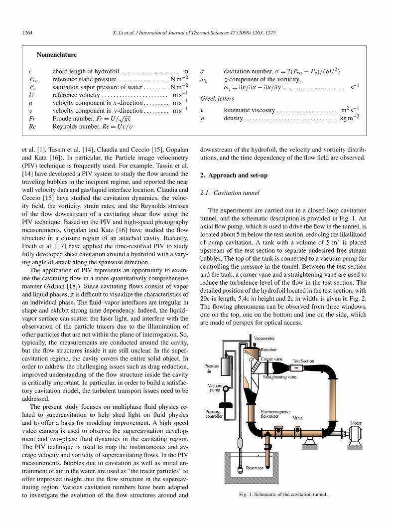
The experiments are carried out in a closed-loop cavitationtunnel, and the schematic description is provided in Fig. 1. Anaxial flow pump, which is used to drive the flow in the tunnel, islocated about 5 m below the test section, reducing the likelihoodof pump cavitation. A tank with a volume of 5 m3 is placedupstream of the test section to separate undesired free streambubbles. The top of the tank is connected to a vacuum pump forcontrolling the pressure in the tunnel. Between the test sectionand the tank, a corner vane and a straightening vane are used toreduce the turbulence level of the flow in the test section. Thedetailed position of the hydrofoil located in the test section, with20c in length, 5.4c in height and 2c in width, is given in Fig. 2.The flowing phenomena can be observed from three windows,one on the top, one on the bottom and one on the side, whichare made of perspex for optical access.

Fig. 1. Schematic of the cavitation tunnel.

X. Li et al. / International Journal of Thermal Sciences 47 (2008) 1263–1275 1265

Fig. 2. Sketch of the foil’s position in the test section.

To ensure the turbulent flow characteristics in the test sec-tion, the flow velocity distributions in the test section without ahydrofoil are measured by LDV (Laser Doppler Velocimetry).The distribution of the average velocities and the turbulenceintensities along the spanwise direction of the test section areshown in Fig. 3. The measurement is conducted when the cav-itation number is 1.29. The data are obtained at three positions:including upstream, downstream and center of the test sec-tion. The average velocities are well-distributed in the measure-mented positions, and the turbulence intensity levels are smallerthan 2% except the near-wall area. Since we capture data onlynear the mid-span area, the measured velocity distributions arelimited near the middle position along Y direction; therefore,the effect from the top and bottom wall can be neglected.

The experimental conditions are maintained to within 1%uncertainty on the hydrofoil angle of incidence and 2% un-certainty on both the flow velocity and the upstream pressure.In detail, an electromagnetic flowmeter, with 0.5% uncertainty,measures the needed velocity; and a pressure transducer, with0.25% uncertainty, monitors the upstream pressure. Together,the cavitation number can be controlled to within 5% uncer-tainty.

In this study, the reference velocity U is fixed at 10 m s−1,the Reynolds number Re is 3.5 × 105, and the Froude numberFr is 17.

2.2. Supercavitating hydrofoil

A hydrofoil investigated by Tulin [19], as shown in Fig. 4,is adopted in the present study. A main feature of this hydro-foil is supercavitation can occur easily. The hydrofoil, with 2cin spanwise direction, is made of stainless steel, and highlysurface-polished. As is clamped on the wall of the test sec-tion with a mechanical locking system, the foil can be fixedat a given angle of incidence. The suction side of the foil ismounted toward the bottom for the convenience of viewing theflowing field. The definition of incidence angle is also presentedin Fig. 4.

2.3. Visualization techniques

The cavitation phenomena are documented by a high-speeddigital camera (HG-LE, by Redlake), up to a rate of 105 framesper second (fps). In order to maintain desirable spatial reso-lutions, much lower recording speed is adopted. Specifically,depending on the focus of the investigation, three rates, namely,50, 2000, and 500 fps are used in this study, respectively. Theexperimental setup is illustrated in Fig. 5. With the flowingfield at the mid-span of the foil illuminated by a continuouslaser beam sheet (LBS) from the bottom wall, the pictures arecaptured and transmitted to the computer in real time for postprocessing.

2.4. Velocity data acquisition

Also as shown in Fig. 5, a 2D-PIV system, manufactured byTSI, is composed of double-pulsed Nd:YAG laser emitting alaser sheet, a PIVCAM 10-30 CCD (Charge Coupled Device)camera with a resolution of 12 bits, 1024 × 1024 pixels col-lecting the instantaneous images, and one type of synchronizerproviding the timing and sequencing of events. The precision of

Fig. 3. Distributions of the average velocity and the turbulence intensity along spanwise direction in the test section (without a hydrofoil).


Fig. 4. Schematic of supercavitation foil.

Fig. 5. Schematic of the layout of the experimental setup.

the whole system is within 0.5 ∼ 2%. The pulse laser sheet isformed with a light-guide arm and shown as a green light band(around 532 nm), with an energy of 50 mJ/pulse at a repetitionrate of 30 Hz.

For two-phase flows, it’s necessary to partition the velocityfields. Grünefeld et al. [20], Boëdec, and Simoëns [21] col-lected both images with different wavelengths using two setsof PIV systems, which combined PIV and laser-induced fluo-rescence (LIF). This is costly due to the additional PIV sys-tem. Furthermore, the uncertainty of measurements increasesdue to interference between different laser sheets, synchroniza-tion of two sets of PIV systems, and choice of two separatetracer particles. For the cavitating flows, appropriate selectionsof tracer particles are particularly critical because (1) the track-ing capability of the tracer particles, which must be of a similardensity to the liquid/gas medium and with small enough ofdiameters, and (2) the cavitating area is defined by irregularly-shaped and time dependent liquid–vapor interface, which canscatter the laser sheet and give incorrect interrogation informa-tion.

On the other hand, in the cavitating flows, the velocity in-formation inside the cavity can also be captured only usingthe vapor bubbles as “tracer particles” (Wosnik and Milosevic[22]). In fact, the free stream carries some air bubbles and thecavitating region consists of numerous vapor bubbles. With thisapproach, both the cavitating flow structure and the measure-ment uncertainty can be assessed.

The commercial PIV-software Insight 2.0 from TSI is usedto process the velocity vector fields with the interrogation areasof 32 × 32 pixels and 50% overlap in general. The images aretreated with two-frame cross-correlation processing. In additionto Fast Fourier Transforms (FFT) and Gaussian algorithm forpeak search, multiple filters have also been employed to removethe erroneous vectors by specifying the relative tolerance untilreasonable results are obtained.

3. Results and discussions

3.1. Multiphase structures associated with supercavitation

In the present study, when the cavitation number is reducedto 0.77 or lower, at 15-degree angle-of-attack, supercavitationis attained and a relatively stable cavity covers the entire hy-drofoil suction surface, extending behind the trailing edge. Inthe supercavitation regime, the different flow patterns appearin response to the variation of the cavitation numbers. Selectedsupercavitation patterns under different cavitation numbers arepresented in Fig. 6. Both original flow visualization illuminatedby a LBS (Fig. 6(a)) and schematic interpretations (Fig. 6(b)),drawn by an in-house feature-recognition software package, arepresented. In the supercavitation regime, there is a distinct inter-face between water and cavitating flow regions, which is calledthe cavity boundary in this study. The cavitating flow patternsexhibit different characteristics in accordance with the cavita-tion numbers. Based on the observations, three stages are shownin the figure, that is: first, fluctuating cavity with periodicalvortex shedding, then, vapor and water–vapor mixture coexistinside the cavity, followed by a turbulent wake, and finally, acavity largely filled with vapor and with a two-phase tail anddistinct phase boundaries in the wake region.

Refer to aforementioned comment on three stages, with thecavitation number of 0.77, the whole cavity is full of water andvapor mixture. As shown in Fig. 7, the flowing structures ex-hibit substantial temporal variations. Generated from the foil’sleading (the lower vortex) and the rear blunt edge (the uppervortex), the cavitation vortices shed from the cavity tail withobvious period. The period is counted between two consecu-tive peak positions of the upper shedding vortices. At the timeof t = 0 ms, the upper cavitation vortex begins to shed as thearrows indicated. An arrow also points out the shedding ofthe lower vortex as t = 4 ms. Several shedding frequencies ofthe vortices are listed in Table 1, according to various record-ing rates. The average shedding frequency—about 129 Hz, isobtained. It can be said that the first stage of supercavitation de-velopment is characterized by fluctuating cavity with periodicvortex shedding.

Further lowering the cavitation number, the cavity becomeslarger and longer, and a transparent area can be observed nearthe hydrofoil suction surface (see, e.g., the case of σ = 0.30 inFig. 6), which indicates that the cavity’s front is largely filledwith vapor. In the condition, the cavitating area consists of twoparts: vapor area in the foreside of the cavity, two-phase mixturearea in the rear region, and a distinct interface between the twozones can be seen. To show it more clearly, the time-evolvedpictures with σ = 0.30 are given in Fig. 8, the arrows in thefigure point out the interface position. Obviously, the interfacelocation is highly unsteady, which indicates a reverse motionfrom two-phase mixture area to vapor area, just like the back-filling process in ventilated supercavitation (Knapp [23]). Afterarriving at the rearward portion of the foil at t = 16 ms, the in-terface continues to move toward the leading edge along the foilsuction section until t = 28 ms, which shows a fully developedbackfilling process. What’s more, various backfilling processes


Fig. 6. Three supercavitating flow structures with different cavitation numbers. In all cases, α = 15◦ . Both flow visualization and schematic interpretation aredepicted.

Fig. 7. Time evolution of the cavity fluctuating and the vortex shedding (σ = 0.77).


Table 1Comparisons of observed vortex shedding dynamics

Recording rate (fps) 2000Shedding 133.33 117.65 142.86 153.85 125.00 105.26 142.86 117.65 133.33Frequency (Hz) 117.65 133.33 117.65 142.86 117.65 153.85 125.00 117.65Average value (Hz) 129.26Recording rate (fps) 500

166.67 125.00 100.00 125.00 166.67 100.00 125.00 125.00 125.00Shedding 125.00 125.00 166.67 100.00 125.00 166.67 125.00 100.00 166.67Frequency (Hz) 100.00 100.00 125.00 125.00 125.00 166.67 100.00 166.67 125.00

125.00 100.00 166.67 125.00 125.00 125.00 125.00Average value (Hz) 128.92

Fig. 8. Time evolution of the interface between vapor and two-phase mixture regions—1 (σ = 0.30).

can be found in the present study. As shown in Fig. 9, the in-terface is divided into two parts: the vertical section in upperpart and the declining section in lower part. While there is a pe-riodic backfilling in the upper region, water–vapor mixture isconverted to vapor in the lower region. Furthermore, the cor-responding backfilling velocities of the interface are estimatedwith normalized data in Fig. 10(a) and (b) respectively. Here,t ′ = t/t∞, t and t∞ (c/U ) are the real time and reference timerespectively, and v′ = v/U∗100%. It can be found that the fluc-tuating ranges of the velocity are kept within 12–25%, i.e., thebackfilling velocity occupies 12–25 percentage of the referencevelocity.

Since the pressure in the transparent vapor area is essen-tially the same as the vapor pressure, and the pressure in themixture region is expected to be higher, the pressure differ-ence induces the time dependency of the interface location.When the interface moves to the left (see Figs. 8 and 9), the va-por region becomes smaller and the two-phase mixture regiongrows. In the process, condensation occurs in the left region,resulting in a higher pressure there. Conversely, as the inter-face moves to the right, the evaporation occurs, and the pressurein the left region is expected to decrease. Under supercavita-tion condition, even though the cavity boundary seems to bequite steady, the pressure fluctuation and unsteady mass trans-fer process can still be substantial inside the cavity, betweenthe vapor and the two-phase regions. Thus, the second stage

of supercavitation development can be characterized as vaporand water–vapor mixture coexist inside the cavity, followed bya turbulent wake.

When the cavitation number further decreases to 0.26, whilestill maintaining the angle-of-attack at 15-degree, the violentfluctuation of the interface between the vapor and the two-phaseregions in the cavity disappears, the cavitation area is largelyfilled with vapor, and the water–vapor mixture only occupies anarrow region, as shown in Fig. 6. The time-evolved pictures areshown in Fig. 11, which exhibit similar features. The same flowpattern persists while the cavitation number is further lowered.In summary, this final stage of supercavitation development canbe characterized as a vapor-filled cavity with a two-phase tailand distinct phase boundaries in the wake region.

3.2. Velocity distributions

The supercavitating and no-cavitating flow fields are mea-sured by double-pulsed PIV images. The concerned flow regionis illuminated by a laser beam sheet from the bottom windowof the test section, as shown in Fig. 12, which gives a double-pulsed images when σ = 0.77. In the experiment, the intervalbetween the image pairs is 50 µs. Based on the velocity vectordata processed in Fig. 13, the following velocity and vorticitydistributions can be obtained through post-processing.


Fig. 9. Time evolution of the interface between vapor and two-phase mixture regions—2 (σ = 0.30).

Fig. 10. Variation of backfilling velocity of the interface.

Fig. 11. Time-evolved supercavitation structures (σ = 0.26).

Fig. 12. Double-pulsed image pairs (σ = 0.77).

3.2.1. Flow structures in no-cavitation conditionThe distributions of flowing fields with no cavitation are

presented in Fig. 14. Fig. 14(a) shows the distribution of thevelocity vectors, and Fig. 14(b) gives the distribution of the vor-

ticity contours. The gray area indicates no laser light entered.Apparently, in the single-phase flows, the whole flowing fieldcan be divided into two areas: (1) In the rearward portion of thefoil-suction section, the velocity is much lower than that in an-other flow region, and extending to form a wake. Thus, this areais characterized as low velocity area. (2) In the other region ex-cept the low velocity area, no large velocity fluctuating occurs.This area is characterized as main stream (free stream) area.

The following characteristics can be observed in the afore-mentioned low velocity area: (a) Two vorticity bands, withpositive and negative direction respectively, are formed. Time-evolved vorticity-contour distributions under no-cavitation con-ditions are presented in Fig. 15. It can be found the position


Fig. 13. The final velocity vector fields (σ = 0.77).

Fig. 14. Distribution of the average characteristics with no cavitation (σ = 2.67).

Fig. 15. Illustration of the instantaneous, z-component vorticity distribution (σ = 2.67).


Fig. 16. Schematic of special locations (σ = 2.67).

from which the vortex is formed remains unchanged, while theirshape and length changes violently, which shows that the vor-ticity distribution of the flowing fields behaves substantial fluc-tuating under no cavitation condition. (b) In order to offer morequantitative information, the average velocity distributions inselected sections, as shown in Fig. 16, are provided in Fig. 17.At the positions of x = 0.5c and x = 1.1c near the foil suctionsection, there are larger velocity fluctuation, in a double-troughshape, while the wakes are quite smooth between x = 1.7c andx = 2.3c.

3.2.2. Velocity distributionsThe average velocity distributions are given in Fig. 18 for

three cavitation numbers: 0.77, 0.30, and 0.26. The velocityvector plots and contours are presented in Fig. 18(a) and (b),respectively. The quantitative velocity distributions in the samesections, as shown in Fig. 16, are provided in Fig. 19. It canbe seen that the velocity distributions in the cavitating regionsare different from those in the bulk flows. Compared to the lowvelocity area in Fig. 14(a), similar characteristics are observedin the cavitation area. However, there is more uniform velocitydistribution in the cavity core, as exhibited by Figs. 17 and 19,e.g., at x = 0.5c and x = 1.1c. In summary, in the cavitatingconditions, with the generation of cavities in the water–vaportwo-phase flow, enhanced momentum transfer between upperand lower flow layers is induced by phase change and cavita-tion dynamics.

Indeed, with the cavitation number decreasing, different fea-tures can be found. As σ = 0.77, the low velocity area extendsalong the whole downstream field with the violent fluctuatingof vortex shedding. When reducing the cavitation number, thelow velocity area becomes smaller, confined between the upperand lower free streams, and the low speed fluid moves towardthe rear region of the cavity.

Fig. 17. Velocity distributions in various sections (σ = 2.67).

3.2.3. Vorticity distributionAround the interface between cavitating and no-cavitating

areas, as discussed by Wang et al. [1], and confirmed by thepresent measurement, a shear flow region exists. The z-compo-nent vorticity distributions can be seen in Fig. 20. As expected,high levels of vorticity are observed around the cavity bound-ary in different cavitating conditions. The vortex bands behavewith obvious stage characteristics with the decreasing of thecavitation number. Firstly, the upper and lower vortex bandsapproach each other with the decreasing of the cavitation num-ber, and extend downstream. Secondly, the position in whichthe lower vortex band form moves back, indicating the inherentrelation between the vortex band and the water–vapor mixture.What’s more, the vorticity is reduced with the decreasing of thecavitation number, just as shown in Fig. 21. To further high-light the cavitation dynamics, time-evolved vorticity-contourdistributions with three cavitation numbers σ = 0.77, σ = 0.30and σ = 0.26 are presented in Figs. 22–24, respectively. Withthe cavitation number σ = 0.77, as shown in Fig. 22, the vor-tex bands almost centralize along the wake flow close to thefoil, although much shorter than that with the cavitation num-ber σ = 2.67. With the cavitation area extending to the wholetest region, the vortex bands become much longer and move tothe right end as shown in Fig. 23. In this stage, correspondingto the traverses of the interface between the vapor phase and themixture phase, changes of the vortex bands area are observed.At the final stage as shown in Fig. 24, the vortex bands appearsteady with less shedding.

3.3. Computational and modeling issues

Regarding future directions, various issues related to super-cavitation should be addressed using combined computationalmodeling and experimental approaches. Specifically, the struc-tures of the three supercavitating flow regimes need to be clari-


Fig. 18. Velocity distribution under different cavitation numbers.

fied. For example, the vortex shedding frequency and the mech-anism about the instability of the interface between the vaporand the two-phase mixture are not well understood. These as-pects seem to be closely related to the interplay between the su-percavitation and the vortex dynamics. A multi-scale model canbe fruitful for treating bubbly flows for finely structured cavi-tating flows. Turbulence modeling needs to be refined to handletwo-phase and compressibility effects. In particular, capabilitiesfor handling the following characteristics are not adequately de-veloped:

i. substantial departure from equilibrium between productionand dissipation of the turbulent kinetic energy,

ii. turbulence-enhanced mass transfer across the liquid–vaporinterface,

iii. momentum transfer between liquid and vapor phases.

The conventional Reynolds-averaged Navier–Stokes ap-proach, even with nonequilibrium effects, may not be adequateto address these challenges. Other than large eddy simulations(LES) and direct numerical simulations (DNS), a hybrid ap-proach such as filter-based RANS model can be useful. As


Fig. 19. The average velocity distributions in special sections.

Fig. 20. The z-component average vorticity distribution in supercavitation conditions.

Fig. 21. The z-component average vorticity distribution under various cavitation numbers.

presented by Johansen et al. [24], and partially evaluated byWu et al. [12] for cavitating flow simulations, the predictivecapability of the current RANS-based engineering turbulenceclosure, conditional averaging can be adopted for the Navier–Stokes equation, with one more parameter, based on the filtersize, introduced into the turbulence model. There are great op-portunities to make progress in the modeling and simulation ofcavitating flows.

4. Conclusions

The multiphase dynamics, velocity, and vorticity distribu-tions associated with supercavitation are presented. The follow-ing is a summary of the main findings:

(1) The cavitation structure depends on the interaction of thewater–vapor mixture and the vapor among the whole su-percavitation stage. Distinct flow regimes are observedwith the decreasing cavitation numbers: (a) first, fluctuatingcavity with periodic vortex shedding; (b) then, vapor andwater–vapor mixture coexist inside the cavity, followed bya turbulent wake; and (c) finally, a cavity largely filled withvapor and with a two-phase tail and distinct phase bound-aries in the wake region.

(2) The interface between the vapor and the two-phase mixtureexhibits substantial unsteadiness, indicating frequent masstransfer processes occurring inside the cavity.

(3) In the supercavitating region, strong momentum transferbetween higher and lower flow layers takes place; velocity




distribution appears even in the core part of the cavitatingregion, and the lower velocity area becomes smaller and,as the cavitation number lowers, moves toward the down-stream.

(4) Around the cavity boundary of the two-phase mixture is ashear layer flow, with a pair of vortex bands formed. Thedevelopment of the lower vortex band is related with the

distribution of the water–vapor mixture. Also, the vorticityreduces with the decreasing of the cavitation number.

Various issues related to supercavitation including the struc-tures of the three supercavitating flow regimes, the vortex shed-ding frequency, and the mechanism about the instability of theinterface between the vapor and the two-phase mixture await to



be addressed based on first-principles computational modelingtechniques.

Acknowledgements

The authors gratefully acknowledge support by the Na-tional Natural Science Foundation of China (NSFC, Grant No.:50276004 and No.: 50679001) and NASA Constellation Uni-versity Institutes Program.

References

[1] G.Y. Wang, I. Senocak, W. Shyy, T. Ikohagi, S.L. Cao, Dynamics of at-tached turbulent cavitating flows, Prog. Aerosp. Sci. 37 (2001) 551–581.

[2] E.P. Rood, Review-mechanisms of cavitation inception, J. Fluids Eng. 113(1991) 163–175.

[3] Y. Kawanami, H. Kato, H. Yamauchi, M. Tanimura, Y. Tagaya, Mecha-nism and control of cloud cavitation, J. Fluids Eng. 119 (1997) 788–794.

[4] A.T. Leger, S.L. Ceccio, Examination of the flow near the leading edge ofattached cavitation, part 1. Detachment of two-dimensional and axisym-metric cavities, J. Fluid Mech. 376 (1998) 61–90.

[5] D.F. Delange, G.J. Debruin, Sheet cavitation and cloud cavitation, re-entrant jet and three-dimensionality, Appl. Sci. Res. 58 (1998) 91–114.

[6] M. Kjeldsen, R.E.A. Arndt, M. Effertz, Spectral characteristics ofsheet/cloud cavitation, Transactions of the ASME, J. Fluids Eng. 122(2000) 481–487.

[7] J.D. Hrubes, High-speed imaging of supercavitating underwater projec-tiles, Exp. Fluids 30 (2001) 57–64.

[8] R. Kuklinski, C. Henoch, J. Castano, Experimental study of ventilatedcavities on dynamic test model, in: Proceedings of Fifth InternationalSymposium on Cavitation (CAV2001), Pasadena, California, USA, 2001,Session B3.004.

[9] Y.T. Wu, D.P. Wang, A wake model for free-streamline flow theory, part 2.Cavity flows past obstacles of arbitrary profile, J. Fluid Mech. 18 (1963)65–93.

[10] R.F. Kunz, D.R. Stinebring, T.S. Chyczewski, J.W. Lindau, H.J. Gibel-ing, S. Venkateswaran, T.R. Govindan, A preconditioned Navier–Stokes

method for two-phase flows with application to cavitation prediction,Comput. Fluids 29 (2000) 849–875.

[11] I. Senocak, W. Shyy, A pressure-based method for turbulent cavitatingflow computation, J. Comput. Phys. 176 (2002) 363–383.

[12] J.Y. Wu, G.Y. Wang, W. Shyy, Time-dependent turbulent cavitating flowcomputations with interfacial transport and filter-based models, Int. J. Nu-mer. Meth. Fluids 49 (2005) 739–761.

[13] A. Hosangadi, V. Ahuja, S. Arunajatesan, A generalized compressiblecavitation model, in: Proceedings of Fifth International Symposium onCavitation (CAV2001), Pasadena, California, USA, 2001, Session B4.003.

[14] A.L. Tassin, C.Y. Li, S.L. Ceccio, L.P. Bernal, Velocity field measurementsof cavitating flows, Exp. Fluids 20 (1995) 125–130.

[15] O. Claudia, S. Ceccio, The Influence of developed cavitation on the flowof a turbulent shear layer, Phys. Fluids 14 (2002) 3414–3431.

[16] S. Gopalan, J. Katz, Flow structure and modeling issues in the closureregion of attached cavitation, Phys. Fluids 12 (2000) 895–911.

[17] E.J. Foeth, C.W.H. Vandoorne, T. Vantersiega, B. Wieneke, Time resolvedPIV and flow visualization of 3D sheet cavitation, Exp. Fluids 40 (2006)503–513.

[18] R.J. Adrian, Twenty years of particle image velocimetry, Exp. Fluids 39(2005) 159–169.

[19] M.P. Tulin, Supercavitating propellers, in: Proceedings of fourth ONRSymp. on Naval Hydrodyn., ONR/ACR-92, Belgium, 2001, pp. 239–286.

[20] G. Grünefeld, H. Finke, J. Bartelheimer, S. Krüger, Probing the velocityfields of gas and liquid phase simultaneously in a two-phase flow, Exp.Fluids 29 (2000) 322–330.

[21] T. Boëdec, S. Simoëns, Instantaneous and simultaneous planar velocityfield measurements of two phases for turbulent mixing of high pressuresprays, Exp. Fluids 31 (2001) 506–518.

[22] M. Wosnik, G. Lucas, R.E.A. Arndt, Measurements in high void fractionturbulent bubbly wakes created by axisymmetric ventilated supercavita-tion, in: Proceedings of ASME Fluids Engineering Division Summer Con-ference, 2005 Forums, FEDSM2005, 2005, pp. 531–538.

[23] R.T. Knapp, J.W. Daily, F.G. Hammitt, Cavitation, McGraw–Hill, NewYork, 1970.

[24] S.T. Johansen, J. Wu, W. Shyy, Filter-based unsteady RANS computa-tions, Int. J. Heat Fluid Flow 25 (2004) 10–21.

structures of supercavitating multiphase flows

Documents