INDEGREE PROJECT ,SECOND CYCLE, 30 CREDITS

,

Structural design and performanceof tube mega frame in arch-shapedhigh-rise buildings

MATISS SAKNE

KTH ROYAL INSTITUTE OF TECHNOLOGYSCHOOL OF ARCHITECTURE AND THE BUILT ENVIRONMENT

DEGREE PROJECT IN CIVIL ENGINEERING, SECOND LEVEL STOCKHOLM, SWEDEN 2017

TRITA-BKN Examensarbete 505, Brobyggnad 2017

ISSN 1103-4297

ISRN KTH/BKN /EX-505-SE

KTH ROYAL INSTITUTE OF TECHNOLOGY

KTH ARCHITECTURE AND THE BUILT ENVIRONMENT

AF223X DEGREE PPROJECT IN STRUCTURAL ENGINEERING AND BRIDGES 2017

Structural design and performance of tube mega frame

in arch-shaped high-rise buildings.

i

Abstract A recent development and innovation in elevator technologies have sprawled interest in how these technologies would affect the forms and shapes of future high-rise buildings. The elevator that uses linear motors instead of ropes and can thus travel horizontally and on inclines is of particular interest. Once the vertical cores are no longer needed for the elevators, new and radical building forms and shapes are anticipated. It is expected that the buildings will have bridges and/or the buildings themselves will structurally perform more like bridges than buildings, therefore this study addresses the following topic - structural design and performance of tube mega frame in arch-shaped high-rise buildings.

Evidently, for a structure of an arched shape, the conventional structural system used in high-rise buildings does not address the structural challenges. On the other hand, The Tubed Mega Frame system developed by Tyréns is designed to support a structural system for high-rise building without the central core, in which the purpose is to transfer all the loads to the ground via the perimeter of the building, making the structure more stable by maximizing the lever arm for the structure. The system has not yet been realized nor tested in realistic circumstances. This thesis aims at evaluating the efficiency of the Tubed Mega Frame system in arched shaped tall buildings. Multiple shapes and type of arches are evaluated to find the best possible selection.

Structural behavior of different arch structures is studied using analytical tools and also finite element method in software SAP2000. The most efficient arch shape is sought to distribute the self-weight of the structure. The analysis shows that it is possible to accurately determine efficient arch shape based on a specific load distribution.

Furthermore, continuing with the arch shape found in previous steps, a 3D finite element model is built and analyzed for linear static, geometric non-linearity (P-Delta) and linear dynamic cases in the ETABS software. For the given scope, the results of the analysis show that the Tubed Mega Frame structural system is potentially feasible and has relatively high lateral stiffness in the plane of the arch, while the out-of-plane lateral stiffness is comparatively smaller. For the service limit state, the maximum story drift ratio is within the limitation of 1/400 for in-plane deformations, while for out-of-plane the comfort criteria limit is exceeded.

ii

iii

Preface

This master thesis has been written at the division of structural design and bridges, department of the Civil and Architectural Engineering, at the Royal Institute of Technology (KTH). The writing process took place in Tyréns, in Stockholm and has been a very rewarding experience. This study concludes two-year Mater’s program at KTH.

I would like to express large appreciation and gratitude to Tyréns and particularly my supervisor Fritz King for providing this great opportunity to conduct my master thesis within an engineering field that I am very much interested in and also for offering his guidance and engineering judgment throughout the whole process.

I also thank my supervisor and examiner Professor Raid Karoumi, for his guidance and inspiration throughout my time in KTH and also for his help, support and feedback throughout the writing process.

Thanks to Mahir Ülker, for his suggestions and knowledge concerning my questions during the process.

Last but not least, I would like to thank the whole working group in Tyréns studying the tube mega frame concept for new building shapes and forms. Thanks to David Desimons, Matea Bradaric for helping with the wind load estimation, also, Grigoris Tsamis, Hamzah Maitham, Levi Grennvall, Sujan Rimal, Lydia Marantou and Paulina Chojnicka for great discussions throughout the process.

Stockholm, June 2017

Matiss Sakne

iv

v

Notations

𝐴 Cross-section area

𝐵 Width of a structural section

𝑏 Width of a cross- section of mega tube

𝑐𝑝𝑤 Windward Coefficient

𝑐𝑝𝑙 Leeward Coefficient

𝐷 Arch bending stiffness

𝐷0 The arch stiffness at the crown

𝐷𝑎 The stiffness at the springing

𝑑𝑥 Horizontal projection of arch element

𝑑𝑦 Vertical projection of arch element

𝐸 Elastic modulus (Young’s modulus)

𝑒1 Eccentricity ratio for wind load (ASCE 7-10 Fig. 27.4-8)

𝑒2 Eccentricity ratio for wind load (ASCE 7-10 Fig. 27.4-8)

𝐹 Transverse load

𝑓𝑐 The cyclic frequency

𝑓 Rise of an arch

𝐺(𝑟) The geometric (P-Delta) stiffness due to the load vector 𝑟

𝐻 Height of a structural section

𝐻𝑞 Horizontal force in the arch

ℎ Height of a cross- section of mega tube

𝐼 The moment of inertia

𝐾 The stiffness matrix

𝐾𝑧𝑡 Topographical Factor

𝐾𝑑 Directionality Factor

𝐿 Theoretical span of an arch

𝑙 Stretched length of a string

𝑙1 Natural length of a string

𝑀𝑠 Moment at the support

𝑀 The diagonal mass matrix

𝑃 Axial load

𝑞(𝑥) Basic load

𝑅 A vector of forces acting at the direction of the structure global displacement

vi

𝑟 The load vector

𝑠 Arc length

𝑇 Period of a Mode

𝑇1 Force at each end of a string

𝑡 Thickness of a cross- section of mega tube

𝑈 A vector of the system global displacements

𝑢 Poison’s Ratio

𝑉 Vertical for in the arch

𝑤 Weight of structural material

𝑥 Horizontal coordinate for the arch

𝑦 Vertical coordinate for the arch

𝑦′ Slope of the tangent line for the arch

𝑦′′ The change of the slope of the tangent line for the arch

𝛼 Thermal expansion coefficient

𝜆 The diagonal matrix of eigenvalues

𝜌(𝑠) Density function for the weight of the chain

𝛷 The matrix of the corresponding eigenvectors (mode Shapes)

𝜑 The angle which tangent to the arc makes with the horizontal axis

𝛹 The matrix of corresponding eigenvectors (Mode shapes)

𝜔 The circular frequency

𝛺2 The diagonal matrix of eigenvalues

vii

Content

1 Introduction .................................................................................................................................... 1

1.1 Background ......................................................................................................................... 1

1.2 Aim and scope ..................................................................................................................... 1

1.3 Assumptions and limitations ............................................................................................... 2

1.4 Method ............................................................................................................................... 2

2 Arch shape and structural behavior................................................................................................. 5

2.1 Arch type ............................................................................................................................. 8

2.2 Arch shape........................................................................................................................... 9

2.2.1 Analytical calculation of the funicular line .......................................................... 11

2.2.2 Numerical calculation of the funicular line ......................................................... 13

2.3 Cross-section variation ...................................................................................................... 14

2.4 Construction technique and sequence.............................................................................. 16

2.4.1 Temporary supports ............................................................................................ 17

2.4.2 Prefabrication ..................................................................................................... 17

3 High-rise structures and Tube mega frame ................................................................................... 19

3.1 High-rise structures ........................................................................................................... 19

3.2 Tube mega frame .............................................................................................................. 20

4 Finite Element Method ................................................................................................................. 21

4.1 Linear elasticity.................................................................................................................. 21

4.2 Structural dynamics ........................................................................................................... 23

4.3 Discrepancies in FEM application ...................................................................................... 23

4.3.1 Material ............................................................................................................... 24

4.3.2 Load .................................................................................................................... 24

4.3.3 Discretization ...................................................................................................... 25

4.4 Finite element types .......................................................................................................... 25

4.4.1 Beam elements ................................................................................................... 25

4.4.2 Shell elements ..................................................................................................... 26

4.5 Construction sequence analysis ........................................................................................ 26

5 Arch Mega Structure ..................................................................................................................... 27

5.1 Introduction ...................................................................................................................... 27

5.1.1 Rules and Regulations ......................................................................................... 27

viii

5.2 Geometry .......................................................................................................................... 28

5.2.1 Cross-sections ..................................................................................................... 28

5.2.2 Support conditions - Foundation ........................................................................ 29

5.2.3 Interactions ......................................................................................................... 29

5.3 Material and Loads ............................................................................................................ 30

5.3.1 Materials ............................................................................................................. 30

5.3.2 Loads ................................................................................................................... 30

5.4 Load Combinations ............................................................................................................ 31

5.5 Quality assurance .............................................................................................................. 32

5.5.1 Model mass ......................................................................................................... 32

5.5.2 Convergence ....................................................................................................... 33

6 Results and discussions ................................................................................................................. 35

6.1 Preliminary arch shape evaluation .................................................................................... 35

6.2 Arch shape and characteristics .......................................................................................... 40

6.3 Bracing system evaluation ................................................................................................. 50

6.4 Arch Mega Structure ......................................................................................................... 53

6.4.1 Deformation ........................................................................................................ 53

6.4.2 Story drift ............................................................................................................ 56

6.4.3 Mode shapes and frequencies ............................................................................ 57

6.4.4 Reaction forces ................................................................................................... 59

6.4.5 Buckling ............................................................................................................... 60

7 Conclusion .................................................................................................................................... 61

8 Further studies .............................................................................................................................. 63

9 References .................................................................................................................................... 65

10 Annex ............................................................................................................................................ 67

10.1 Annex A ............................................................................................................................. 67

10.2 Annex C ............................................................................................................................. 68

10.3 Annex D ............................................................................................................................. 72

10.4 Annex E ............................................................................................................................. 73

1

1 Introduction

1.1 Background

Company Tyrens, the Council on Tall Buildings and Urban Habitat and ThyssenKrupp have formed an architectural and structural engineering group to study the effects of shared-shaft elevator technologies on the forms and shapes of high-rise buildings.

ThyssenKrupp is developing an elevator that uses linear motors instead of ropes and can thus travel horizontally and on inclines. Once the vertical cores are no longer needed for the elevators new and radical building forms and shapes are anticipated. These new buildings will begin a new era in building forms. It is expected that the buildings will have bridges and/or the buildings themselves will structurally perform more like bridges than buildings.

Based on these novel ideas it is of high interest to evaluate the structural performance of these new building shapes and forms. By eliminating the need for vertical elevator shafts, which also functioned as the main structural stability elements for conventional high-rise structures, it is possible to consider different and new novel ways of stabilizing the structure. One such concept is the tube mega frame (TMF), which essentially provides the structural integrity of the structure on building perimeter and eliminates the central core.

The tube mega frame concept has been studied for more conventional high-rise shapes and proven to be by all means a structurally sound concept. Therefore, as further development of the TMF, it would be of interest to evaluate, whether or to what extent this concept would perform well with the new building shapes and forms. With initial structural restrictions limiting architectural designs, now it is of interest to evaluate where the new limitation lies.

For the thesis at hand, an evaluation of the structural performance of a novel architectural design of high-rise structure is performed. The structural shape takes a form of an arch. Arched megastructures have been commonly used in the construction of bridges and stadium roofs, where the span of the structure is usually much longer than the height. For this particular thesis, the other end of the spectrum is studied, where the height of the structure is greater than the span, allowing for the structure to enter the realms of high-rise structure.

Arched structures can take various forms and shapes, therefore, a thorough investigation of the optimal geometry is performed, which essentially leads to reduced material consumption and preferable construction sequence and, most importantly, demonstrate that such a structure can be realized under the right circumstances.

1.2 Aim and scope

The aim of the study is to evaluate an arch structure and its suitability for tall building application, in particular, using tube mega frame concept. In order to demonstrate the structural performance the study focuses on indicating relevant parameters that are vital for arched structures and play a major role in the efficiency of the structural system. Parameters influencing the shape of the structure, force distribution within the structure as well as the effect of different bracing systems are to be evaluated. Furthermore, the emphasis is put on demonstrating the continuity between the results of analytical and numerical calculation with finite element models.

2

1.3 Assumptions and limitations

The study only considers one prototype of an arch structure. Different parameters are studied on various levels of complexity in order to define the structural elements of the structural system. Material nonlinearity is not considered. The effects of creep, shrinkage or temperature have not been analyzed for concrete. A limited amount of the loads are included in the study. Loads such as installation loads and façade loads among others are not considered. The assessment of the structure system using finite element method is limited to linear static load conditions, geometric non-linear conditions (P-Delta) and linear dynamic load conditions.

1.4 Method

LITERATURE STUDY

Literature study serves the purpose of acquisition of knowledge. As a part of the revision, brief history and structural principles of arch structures are studied, which essentially set the basis for the particular arch structure under consideration. Also, structural design principles of Tubed Mega Frame concept are investigated through previous publications, allowing for a qualitative estimation of the preferable structural system. Finite Element Method is briefly included in the literature study as it is selected as the main tool for the analysis. Through the literature review the strengths, but most importantly sources of error and limitations of FEM are highlighted to provide an understanding of potential drawbacks of more complex models.

FINITE ELEMENT METHOD

The study primarily uses finite element method to model and analyses the structure. The analysis is performed on multiple scales of complexity in ascending manner. This particular setting allows for better understanding and overall control of the models. For simpler models, equivalent analytical solution procedures are available, therefore, allowing for quality verification tools. Furthermore, results in more complex models can be traced back and must be comparable to ones in simpler models.

PRELIMINARY ARCH SHAPE EVALUATION

An evaluation of common arch shapes based on presented functions is performed. For constant material and cross-sectional geometry properties as well as a constant span to rise ratio - linear, parabolic, catenary and arc shapes are evaluated in terms of support reactions and also relative buckling safety. The evaluation is performed using FEM software SAP2000, structures are analyzed using self-weight of the structure.

ARCH SHAPE CALCULATION

The arch shape is calculated by numerical iterative procedure, where the self-weight distribution within the structure is accounted for. Cross-sectional variation is applied by enforcing initial assumption upon the structural elements, particularly, varying cross-section height. For the acquired arch shape, few options are examined relating to mega tube location with respect to one another and the centerline of the arch shape. The evaluation is performed using FEM software SAP2000, structures are analyzed using self-weight of the structure. Available quantities from the numerical iterative procedure are evaluated with the results of FEM. Elastic modulus for the megastructure is kept constant as well as the thickness of the tube section. For more detailed information on the calculation procedure see section 2.

3

BRACING SYSTEM EVALUATION

An evaluation of different bracing systems is performed for specified tube mega frame arrangement. 2D FEM in SAP2000 is used to assess the deformation of the structure, buckling safety as well as mode shapes and frequencies. Three different bracing arrangements are evaluated to one another by having equivalent weight, which include some of the most common principles for typical bracing systems. X-BRACING system consist of common steel braces arranged in cross formation, F-BRACING utilizes the principles of steel moment frames, and B-BRACING includes steel truss principles at certain heights along the building. The evaluation more thoroughly examines three types of bracing systems for in-plane performance.

STATIC ANALYSIS

The 3D arch mega structure is evaluated using static analysis, which is implemented using finite element analysis software ETABS considering both linear static and non-linear static cases. The geometry of the finite element model is based on the results of the preliminary studies. Estimated loads are applied to the model and linear static analysis is performed. For geometric non-linearity analysis, P-delta effects are considered. The P-delta effects are considered as a separate load case in ETABS and analyzed as the initial load case. Upon converged results, for P-delta effects the stiffness of the model is further used for the analysis of remaining linear static cases. The assessment of the results includes self-weight of the whole structure, reaction force at the base, story drift ratios, and the deflections of the structure. Also, forces in structural elements are evaluated including the effects of P-delta. Buckling safety of megastructure is evaluated.

DYNAMIC ANALYSIS

Dynamic analysis is performed within the same finite element model and includes Modal analysis. From the modal analysis, the natural frequencies and periods of the building are obtained which allow for the evaluation of the overall stiffness of the structure.

4

5

2 Arch shape and structural behavior

Arched structures have been used for various purposes and have been around for a long time. These structures provide very efficient transfer of forces if designed accordingly. The very first structures that resemble an arch were built in form of so-called “corbelled arch” (1). The structural behavior of these structures produce no horizontal force at the supports, however, for larger spans, extensive height is required.

Shortly after the “corbelled arch”, the use of “vault” structures emerged. These structures were built in a way to only support compressive forces, mainly, due to construction technique and material availability at the time. These type of structures were constructed using bricks or stones, with very weak or no binding material in between. The main and only difference between an arch, as we know it today, and a vault is that arches can withstand tensile forces within the structure, however, arches at times are designed to resemble vaults and the difference between the two often are somewhat blurred. (1)

Structures which employ vaults are known to be preserved from around 1000 BC (1), however, the Romans were the first to construct major structures utilizing the principles of an arch in the form of barrel vault, as shown in Figure 2.1. At the time structures like bridges, aqueducts and roof structures were constructed in this way (2).

Gothic arches emerged through Middle Ages, characterized by the pointed apex, and were extensively used in the construction of European cathedrals. These types of arches still functioned in compression, however, they had the tendency to produce large horizontal forces at the supports, also called springing. For the structure to work it was necessary to construct heavy structures that would withstand the horizontal force, without a collapse, therefore frequently flying buttresses were constructed to fulfill this function. (2)

In the 18th century, many bridges were designed and built utilizing masonry vault structures, as shown in Figure 2.2. Many of these bridges have been conserved to this day and carry the load that is vastly greater that the ones, that these structures were intended for at the time. (2) Substantial research has been conducted on these types of bridges and recently it has been possible to show that the interaction with the filling material greatly increases the strength of the bridge, hence, clarifying the strength and durability phenomena of these structures. (1)

When an unrestricted approach is taken when designing arched structures the word “arch” is used. For such structures materials with sufficient tensile capacity are required. Most common arches are of reinforced concrete, steel or laminated timber (Glulam), although in theory many materials could be used. (1)

Figure 2.1 – Roman barrel vault arch structure

Figure 2.2 – Masonry bridge vault structure (1)

6

Among the evident economic advantages, these structures give unique visual experience. They have been used in various shapes to get across the intended aesthetic impression for specific buildings.

Nowadays most new built arched mega structures can be observed in many bridge structures. As per (1) the development of the arch spans has increased considerably over past century, due to technological advances and increased understanding and knowledge of structural behavior. Nowadays the longest spans reach 552 m for steel structures and 445 m for concrete structures. See Annex D for a full list of largest arch bridges. Arch mega structures are common to use in stadium roof construction and massive dam constructions as well.

Another great structure, where the principles of the concept of the ideal arch shape, or at least the quest in pursuit of the ideal aesthetic and structurally honest arch shape is present is the Gateway Arch – The Jefferson Memorial dedicated to Thomas Jefferson – to his vision of an America stretching across the continent, and his Louisiana Purchase, which roughly doubled the size of America at the time. This magnificent structure constructed in the shape of an arch is among the highest arch structures ever built, considering the rise of an arch. In the context of the present study this monumental structure draws undeniable similarities, therefore, a more thorough look is taken to examine the origins of the shape and design principles of the Gateway Arch.

Although there has been some initial confusion about the shape of the arch, it has since been determined and proved that the arch takes the shape of a so-called weighted catenary. Very simply put, the arch resembles the shape of a hanging chain with varying size of the chain links. More thorough discussion on arch shapes is presented further on in this study.

The size of an arch is 630 feet (192 m) high and 630 feet (192 m) wide forming the aspect ratio of 1:1. The term aspect ratio in this context describes no more that the width to height ratio of an arch structure. These aspect ratios are not typically used for arch bridges, dams or stadium roof trusses, instead, these structures strive for more shallow arch shapes with aspect ratios of around 5:1. This notion by itself arises design challenges that are quite different from the ones in more shallow arch megastructures, however, in general “it may be worth noting that the 1:1 aspect ratio is a very old tradition in architecture. In medieval times, it was known as ad quadratum. The original 1386 specification for the cathedral of Milan is an example”. (3)

Chaotianmen

Lupo HuangpuNew River Gorge

Bayonne Kill van Kull

Wupper BridgeEads Bridge

0

100

200

300

400

500

600

700

1700 1800 1900 2000

Max

. SP

AN

[m

]

Figure 2.3 - Largest arch bridges from 18th century to nowadays

Figure 2.4 - Eero Saarinen’s Gateway Arch, St. Louis.

Image reproduced from (3)

7

R. Osserman has studied the trade-offs between the mathematical and esthetical reasoning behind the description of the shape of the Gateway Arch and in his work, has provided some general notions concerning the relation between the formulation of hanging chain and that of an arch.

“It was Robert Hooke who in 1675 made the connection between the ideal shape of an arch and that of a hanging chain in an aphorism that says, in abbreviated form, “As hangs the chain, so stands the arch.” In other words, the geometry of a standing arch should mirror that of a hanging chain.” (4)

He has decisively concluded that the aesthetic and structural decisions that have to be made when designing an arch are “inextricably entwined”. This statement, however, is not surprising and is repeatedly addressed in this study as well.

Once the fact that the hanging chain and an arch being similar, is established, it is evident that analogous issues have to be addressed. The quest for finding the ideal shape has to be commenced. The history of the problem has been clearly presented in R. Osserman’s research, therefore it is recommended to see (3) and (4) for further insight.

In general, the term catenary is used when describing the shape of a hanging cable under its own weight. Evidently, the function describing the cable is derived based on the weight density1 of the cable. In structural mechanics2, the catenary can be described using the theory of elastic strings, which is based on the Hook’s law3. This theory describes the elongation of a string under tensile forces and only considers axial deformations. (5)

𝑙 − 𝑙1 = 𝑙1𝑇1

𝐸 ( 2-1 )

Where l is the stretched length of a string, l1 natural length, 𝑇1 the force at each end of a string, E elastic modulus (Young’s modulus).

“This law governs the extension of other substances besides elastic strings. It applies also to the compression and elongation of elastic roads.” (5)

“This law is true only when the extension does not exceed certain limits, called the limits of elasticity. When stretching is too great the body either breaks or receives such a permanent change of structure that it does not return to its original length when the stretching force is removed.” (Routh Art. 490)

Using theory of elastic strings, it is possible to calculate force equilibrium when the cable is subjected to any load and also to its own weight.

“It is shown that the equilibrium of an arch is achieved by combining forces at the points of an arch and, similarly to hanging chain, the horizontal component of the force is constant and simply transmitted along the arch or chain, while the vertical forces are mirror images.” (4)

An important aspect when using elastic string theory is to understand that the basis of this theory originates around tensile axial deformation and in no way, consider bending stiffness of a string,

1 Weight density - the weight per unit volume of a substance or object. (www.dictionary.com 28.03.2017)

2 Structural mechanics or Mechanics of structures is the computation of deformations, deflections, and internal forces or stresses (stress equivalents) within structures, either for design or for performance evaluation of existing structures. (Wikipedia 28.03.2017)

3 Hook’s law - is a principle of physics that states that the force (F) needed to extend or compress a spring by some distance X is proportional to that distance. That is: F = kX, where k is a constant factor characteristic of the spring: its stiffness, and X is small compared to the total possible deformation of the spring. The law is named after 17th-century British physicist Robert Hooke. (Wikipedia 28.03.2017)

8

therefore, it is reasonable to believe that the accuracy of this theory, when used for arch structure, will not reflect the real behavior, especially, when structure is designed to have significant bending stiffness.

The procedure of finding the shape of the structure, however, is a sound concept, and similarly, for an arch structure, the shape can be derived based on the weight density of the structure.

2.1 Arch type

From the perspective of structural definition, arches often are categorized by their structural system. In (1) H. Sundquist uses terms “single-hinge”, “two-hinge”, “three-hinge” and “zero-hinge” arch referring to statical determinacy of the system. In Figure 2.5, it is possible to observe the notations used when describing an arch from a structural perspective. The respective arch lines represent the center-of-gravity lines for the arches. Each of these types has their own advantages and, therefore, the choice of a system for a particular case is based on the actual conditions. The major contributing factors are foundation condition and construction method, which will eventually determine the structural design.

Zero-hinge arches require good foundation conditions, also for most cases reinforced concrete material would be the most economic choice, although steel has the advantage in cases where complex construction sequences have to be resorted to. Under sufficient conditions, especially for large spans, it is appropriate to choose zero-hinge arch, since this leads to reduced consumption of material for the megastructure, provided that the cross-sectional variation is resorted to. (1)

“The relationship is illustrated in Table 2.1, which applies for an evenly distributed variable load p and which indicates the maximum moment, the average value of the maximum moment curve and the relative buckling safety for a given section at the crown and a given load. The Table 2.1 shows that the zero-hinge arch has the lowest average moment and thus the lowest material consumption. At the same time, it has the greatest buckling safety, which permits slender dimensions and less weight for large spans.” (1)

Table 2.1 – Comparison of different arch types (1)

ARCH TYPE CROSS-SECTION VARIATION MAX. MOMENT AVERAGE MAX. MOMENT RELATIVE BUCKLING SAFETY

3-HINGE - ± 0,0188pL² ± 0,0125pL² 1,00

2-HINGE D = EI cos φ = D0 ± 0,0166pL² ± 0,0116pL² 1,33

0-HINGE Kararnowsky-type ± 0,0218pL² ± 0,0071pL² 3,28

Based on the knowledge of the structural definition, the study will focus on the zero-hinge arch, as it is expected that the sheer scale of the structure will require efficient design and solid foundation, therefore, an assumption is made that at this instance foundation is in good enough condition to support a zero-hinge structure.

Figure 2.5 - Arch types with respect to the number of hinges together with notations. (1)

9

2.2 Arch shape

As mentioned before the shape of the Gateway Arch is a weighted catenary, although it has been confused with catenary and parabola instead. It is not, however, something that visually is easily distinguishable, although the mathematical formulation is quite different. Parabola is a function of the single-variable quadratic polynomial ( 2-2 ), the catenary is a function of hyperbolic cosine ( 2-3 ), while weighted catenary is a function of hyperbolic cosine ( 2-4 ) but includes constants that allow for shrinking of the curve.

𝑓(𝑥) = 𝑎𝑥2 + 𝑏𝑥 + 𝑐 ( 2-2 )

𝑓(𝑥) = 𝑎 ∙ cosh (𝑥

𝑎) =

𝑎(𝑒𝑥𝑎+𝑒

−𝑥𝑎)

2 ( 2-3 )

𝑓(𝑥) = 𝑏 ∙ cosh (𝑥

𝑎) =

𝑏(𝑒𝑥𝑎+𝑒

−𝑥𝑎)

2 ( 2-4 )

“The term “weighted catenary” conveys essentially no useful information; virtually any curve that one can picture as a possible candidate for weighted catenary can actually be reproduced by a suitably weighted chain. Furthermore, it is not descriptive, in that it says nothing about the actual shape of the arch, but only about the method used to produce it.” (3) Rather than using the term weighted catenary, R. Osserman uses the term flattened catenary. “In short, a “pure catenary” is the ideal shape for an arch of uniform thickness, and a flattened catenary is an ideal shape for an arch that is tapered in certain precise (and elementary) manner.” (3) Further, the term flattened catenary is adopted and resorted to whenever describing a tapered catenary.

In the case of weighted chain, R. Osserman puts forward equation for expressing the amount of the weight of the chain by a density function ρ(s) , where the weight of any arc of the chain is the integral of ρ(s) with respect to arc lengths over the arc. Osserman shows that a given flattened catenary of the form

𝑓(𝑥) = 𝐴 ∙ 𝑐𝑜𝑠ℎ(𝐵 ∙ 𝑥) + 𝐶 ( 2-5 )

Is obtained from the density function 𝜌 which, when expressed in terms of 𝑥, takes the form:

𝜌(𝑠(𝑥)) = (𝑎𝑦+𝑏)

𝑑𝑠

𝑑𝑥

= (𝑎𝑓(𝑥)+𝑏)

√1+(𝑓′(𝑥))2 ( 2-6 )

Where the coefficients a and b are determined by the coefficients A, B, C of 𝑓(𝑥), up to an arbitrary multiple since multiplying the density by an arbitrary positive constant just changes the total weight, but not the shape of a hanging chain. The physical meaning of this is that the weight of any portion of the chain laying over a segment of the x-axis, given by ∫ 𝜌(𝑠)𝑑𝑠, is equal to ∫ 𝜌(𝑎𝑦 + 𝑏)𝑑𝑥 over the given x-interval, hence providing a method for estimation of arch shape based on its weight density.

The weight of the structure defines the most efficient shape of transferring the weight to the foundation, however, another important aspect that greatly affects the shape is the aspect ratio. By changing the aspect ratio, it is possible to either minimize the effects of weight distribution in defining the shape of the structure or highly increase these effects.

10

Also, a great discussion is brought up by R. Osserman about the influence of aspect ratio on the perception of the structure but more importantly differences between previously mentioned functions that are likely to mathematically describe the ideal shape for an arch. As he points out and also as can be observed in Figure 2.6 and Figure 2.7 the difference between the catenary and the parabola becomes indistinguishable as the aspect ratio increases, on the other hand, the differences are undeniable for smaller aspect ratios. The takeaway from these observations is that for shallower arches one can get away with using almost any of previously mentioned functions to describe the shape of the arch and still be relatively close to the ideal shape for the arch, however, if one wants to be more accurate in finding the ideal shape for an arch with a small aspect ratio, it will be of utmost importance to resort to the function of flattened catenary to mathematically describe the shape.

Figure 2.7 - Different functions (aspect ratio 4:1)

An aspect ratio is somewhat more an aesthetic tool that will affect the visual perception of an arch. As discussed before, the structural design of an arch could be seen through for various aspect ratios. Further in this study, the parameters affected by aspect ratio are discussed, however, the choice of aspect ratio for the arch evaluated will be based on more of an aesthetic motivation.

The ideal shape of an arch is a key concept and, therefore perhaps a more thorough explanation should be given to grasp the context. H. Sundquist has used term “funicular line” to describe the ideal shape. The funicular line also known as a compression line is a factious curve which connects load position so that only compression forces occur in the arch. When the arch shape coincides with the funicular line – no moments in the arch arise. It must be reminded that the funicular line is determined for one specific load situation and for all other loading combinations bending moments are likely to occur in the arch. For example, for a point load at the crown, the funicular line would be triangular, while for a uniformly

Numerical Parabola Catenary Flattened catenary

Numerical

Parabola

Catenary

Flattenedcatenary

Figure 2.6 - Different functions (aspect ratio 3:4)

11

distributed load (second-degree parabola) the funicular line would be parabolic. R. Osserman points out an interesting phenomenon, that if one would design an arch to take parabolic shape, since following Hooke’s dictum, in that case, it would require the greatest weight at the crown, and therefore an arch that was thickest at the top and slimming down toward the bottom, which is counterintuitive with what would be required from structural point of view.

It is also noted that the process of calculating the fully three-dimensional shape of the Gateway Arch was somewhat different from the more common approach of starting with a hanging chain and adopting the form it takes in order to build an arch. In this particular case, the desired shape was settled upon first and thereafter the degree of tapering was determined that would fit the shape from a structural perspective. Although different, the process still involved the same parameters and concepts. The relation between the weight distribution in the arch and the ideal shape are directly correlated.

2.2.1 Analytical calculation of the funicular line

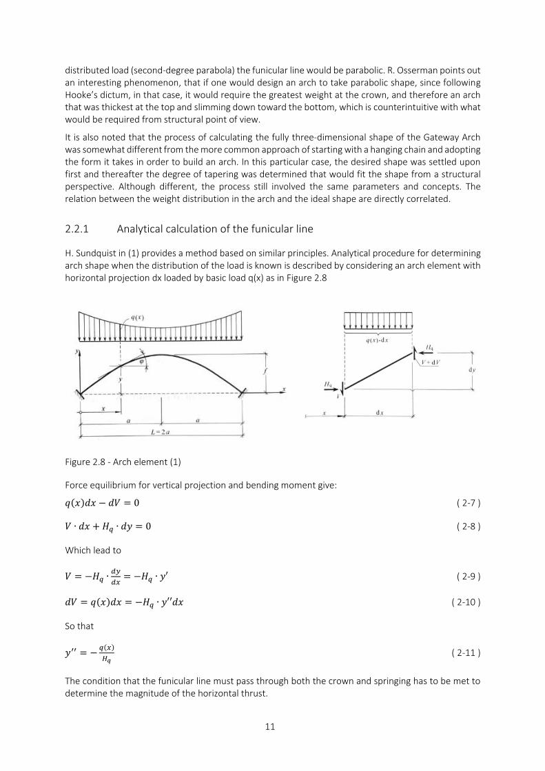
H. Sundquist in (1) provides a method based on similar principles. Analytical procedure for determining arch shape when the distribution of the load is known is described by considering an arch element with horizontal projection dx loaded by basic load q(x) as in Figure 2.8

Figure 2.8 - Arch element (1)

Force equilibrium for vertical projection and bending moment give:

𝑞(𝑥)𝑑𝑥 − 𝑑𝑉 = 0 ( 2-7 )

𝑉 ∙ 𝑑𝑥 + 𝐻𝑞 ∙ 𝑑𝑦 = 0 ( 2-8 )

Which lead to

𝑉 = −𝐻𝑞 ∙𝑑𝑦

𝑑𝑥= −𝐻𝑞 ∙ 𝑦′ ( 2-9 )

𝑑𝑉 = 𝑞(𝑥)𝑑𝑥 = −𝐻𝑞 ∙ 𝑦′′𝑑𝑥 ( 2-10 )

So that

𝑦′′ = −𝑞(𝑥)

𝐻𝑞 ( 2-11 )

The condition that the funicular line must pass through both the crown and springing has to be met to determine the magnitude of the horizontal thrust.

12

The analytical funicular line in Figure 2.10 is derived for parabolic load approximation according to (1) illustrated in Figure 2.9. One can observe that the funicular line “raises its back” (1) the more the basic load increases towards the springing. It is also noted that in many cases, the basic load can be approximated by a parabolic function as shown in Figure 2.9.

Figure 2.9 – Parabolically varying basic load 𝑞(𝑥) = 𝑞(𝑢) = 𝑞0 + ∆𝑞(1 − 𝑢)2. (1)

Although the parabolic function is a good approximation for the basic load, it is not the exact solution. A different procedure is required in order to more accurately determine the funicular curve for the basic load when the load variation is more complex and cannot be directly estimated by known mathematical function.

The closer the structure resembles the funicular curve for the specific loading case the smaller the effect of bending moments in the structure, which in general leads to more optimized structures and reduced material consumption.

When evaluating the influence of span/raise ratios on parabolic load approximation of a basic load distribution it can be observed in Figure 2.11, that the load magnitude increases rapidly towards the springing as the span/raise ratio decreases. Such relationship can be expected based on the load estimation principles mentioned previously.

0.0

0.1

0.2

0.3

0.4

0.5

0.6

0.7

0.8

0.9

1.0

0.0 0.1 0.2 0.3 0.4 0.5 0.6 0.7 0.8 0.9 1.0

y/f

x/L

1

2

4

9

∆𝑞/𝑞0

Figure 2.10 - The shape of the funicular curve for different distributions of the load.

13

Figure 2.11 - Basic load distribution for different span/raise ratios (constant cross-section area)

If the ratio of load increase at springing with respect to the load at the crown is considered, it is possible to observe in Figure 2.12 that the ratio decreases exponentially as the span to raise ratio increases.

Figure 2.12 - Δq/q0 at springing for different span/raise ratios (constant cross-section area)

2.2.2 Numerical calculation of the funicular line

The geometric shape of an arch greatly affects the functionality, design, and performance of the structure. The key to quality design is to define a shape that closely follows the natural path of forces through the structure, in this way leading to the fundamental basic concept of an arch in that it shall primarily function as a structure under pure axial pressure.

Any arch can be designed to function purely under compressive forces for a particular basic load q. Usually, the basic load is preferred to be a self-weight of the structure as this type of action is permanent on any structure.

The process of defining the structural shape, however, takes thorough consideration in early stages in the design process. It is clear, that it will not be possible to design a structure to act purely in compression for all loading situations, and since the self-weight of the megastructure accounts for large part of the force exerted on the structure, a sensible approach is to design the structure close to the funicular shape for the self-weigh of the structure. To compute the funicular line for self-weight (1) provides a methodology in which an iterative procedure is used. “Numerical determination of the funicular line where the shape of this line is dependent on the load, and where the load, in turn, is

0.0

2.0

4.0

6.0

8.0

10.0

12.0

14.0

16.0

0.0 0.1 0.2 0.3 0.4 0.5 0.6 0.7 0.8 0.9 1.0

q(x

)/q

0

x/L

0,50

0,75

1,00

1,50

5,00

𝐿/𝑓

1.0

2.0

4.0

8.0

16.0

32.0

64.0

128.0

0.0 0.5 1.0 1.5 2.0 2.5 3.0 3.5 4.0 4.5 5.0

Δq

/q0

L/f

14

dependent on the arch shape.” (1) At times, multiple iteration steps are required to acquire converged result. The amount of these steps depends on the quality of the first estimate of the form of the funicular line.

Rather than attempting to find an analytical solution to define the shape of an arch, it is possible to resort to the numerical calculation to determine the funicular line. A common way of implementing this procedure is by using numerical integration of ( 2-11 ). The accuracy of this solution can be adjusted by the amount of discretization of the calculation model. Trapezoidal rule is used for the integration. This procedure allows for easy incorporation computer software.

To construct a funicular curve, the load arrangement of the self-weight of the structure must be estimated. One advantage of this procedure is that the first estimation, even if not very accurate, will only increase the iteration steps required to arrive at desired accuracy for funicular line, therefore one can start by assuming a parabolic shape, which, if we consider the previous discussion, will certainly not be close to funicular line for this structure, but gives a rather easy way to define a shape which fits the overall rise and span set out for the arch.

This study resort to the numerical calculation procedure in order to determine the shape of the arch. This procedure leads to the development of practical tools in MATLAB in order to make the calculation quick and also the further implementation in the FEM software is made more fluent in this way.

2.3 Cross-section variation

The cross-sectional variation of the arch is influenced by various variables. The choice of the material, the span, construction techniques and maintenance consideration play a significant role in the design process. Also, the way in which the load is transferred into the structure is vital. The choices for cross-sectional design must take into consideration economic aspects of the design and assembly. In general, it is beneficial to maintain a lower weight for the structure, however, the design must not lead to a complex design, which would rapidly outweigh the benefits of the lower weight. (1)

For long spans, it is of interest to have more sophisticated cross-section variation. As the forces increase towards the springing it should be reasonable to increase the cross-sectional dimensions in regions with higher force concentrations, as can be observed in Figure 2.13.

Figure 2.13 - Notations for bending stiffness of zero-hinge arch (1)

Arch bending stiffness is expressed as

𝐷 = 𝐸𝐼 cos(𝜑) ( 2-12 )

Where E is the modulus of elasticity, 𝐼 is the moment of inertia and 𝜑 is the angle which tangent to the arc makes with the horizontal axis.

15

Cross-sectional variation methods mentioned by (1) provides few different possibilities of describing the variation. Strassner variation presents a case wherein ( 2-13 ) k = 1 while Ritter using the same ( 2-13 ) presents a case with k = 2, both are given for different values of n = D0/Da.

𝐷(𝑥)

𝐷0=

𝐸(𝑥)𝐼(𝑥) cos(𝜑(𝑥))

𝐸𝐼0=

1

1−(1−𝐷𝑎𝐷0

)(1−2𝑥

𝐿)

𝑘 ( 2-13 )

Kasarnowsky has produced the case for variation in stiffness which is described by:

𝐷(𝑥)

𝐷0=

𝐷𝑎

𝐷0(1 −

2𝑥

𝐿)

4 𝑓𝑜𝑟 0 < 𝑥 <

𝐿

2(1 − √

𝐷𝑎

𝐷0

4) ( 2-14 )

𝐷(𝑥)

𝐷0= 1 ,00 𝑓𝑜𝑟

𝐿

2(1 − √

𝐷𝑎

𝐷0

4) < 𝑥 <

𝐿

2 ( 2-15 )

Where 𝐷0 is the arch stiffness at the crown and 𝐷𝑎 is the stiffness at the springing.

The advantages of using one or the other variation strongly depend on the limitations that occur on the site, especially the condition of the foundation, other than that the variation type will determine the force distribution within the structure.

In Figure 2.14 one can observe an example of the comparison of the cross-sectional variation methods.

Figure 2.14 – Examples of cross-section variation when the stiffness ratio between the crown and springing is 𝐷𝑎/𝐷0 = 3 (1)

The advantage of using predefined cross-section variation is that for these particular cases structural engineers have developed analytical solutions for force distribution within the structure, which can serve as a beneficial tool for verification of calculation models.

0.00

0.50

1.00

1.50

2.00

2.50

3.00

0.0

0

0.0

5

0.1

0

0.1

5

0.2

0

0.2

5

0.3

0

0.3

5

0.4

0

0.4

5

0.5

0

Dx/

D0

x/LStrassner Ritter Kasarowsky

16

2.4 Construction technique and sequence

It is expensive and complicated to construct the formwork and scaffolding for casting large concrete arch structures. Formwork for arch bridges is costly, various methods for rational formwork and assembly of arches have, therefore, been developed, see Figure 2.15. (1)

Types of formwork

Conventional formwork with shoring

Formwork suspended in hangers

Simply supported formwork

Statically interacting formwork

Cantilever building procedures

The “Freivoorbau” method with suspended formwork

The “Freivoorbau” method with combined shoring suspended formwork

The “Freivoorbau” method with a truss supporting system

Suspended formwork approach

Figure 2.15 – Examples of construction procedures for arch bridges. (1)

The construction method, temporary support system and formwork largely affect the economic feasibility of building an arch structure. More so, the choice will affect the design procedure and principles. Stresses that accumulate during construction stages largely affect the structure and eventually the performance of the structure in exploitation. Without knowing exact steps in the construction sequence, it will be difficult to complete a thorough structural assessment analysis and provide accurately design structural components.

17

2.4.1 Temporary supports

Figure 2.16 illustrate a method which has been implemented in a construction process of an arch structure. The procedure follows the sequence where the foundation for the cast stages nearest to the supports is papered and the formwork is built with help of conventional form towers and a special truss system. Followed by temporary formwork with caissons is prepared and towers are erected on these. The subsequent construction is done with cables as support. (1)

Figure 2.16 - Example of construction sequence of an arch bridge. (1)

This procedure might be difficult to apply for arches having lower aspect ratios, therefore, adequate methods likely have to be considered.

2.4.2 Prefabrication

Assembly of the arch structure is expected to be a lengthy process, more so, if concrete formwork is of varying nature so that it has to be adjusted for every consecutive stage. Evidently, this would largely affect the feasibility of the whole construction. A prefabrication process in these instances would be beneficial. A great example addressing this issue was used in The Gateway Arch construction. It was done by prefabricating stainless steel outer shells, which then would be assembled on site and filled with concrete, in this way avoiding time-consuming framework issues. While addressing some issues, other might have arisen, therefore, it is of utmost importance to evaluate all aspects of such a construction project to find the middle ground.

18

19

3 High-rise structures and Tube mega frame

3.1 High-rise structures

There is no absolute definition of what constitutes a “tall building” or a high-rise structure according to the Council of Tall Buildings and Urban Habitat (CTBUH), however, several criteria can be evaluated to establish whether a structure would qualify as one. Amongst the important aspects are height relative to context, proportions of the structure and tall building technologies. In more general terms, “The CTBUH defines “supertall” as a building over 300 meters (984 feet) in height, and a “mega tall” as a building over 600 meters (1,968 feet) in height. As of June 2015, there was 91 super tall and 2 mega tall buildings fully completed and occupied globally.” (6)

“In 2016, 128 buildings of 200 meters’ height or greater were completed, setting a new record for annual tall building completions and marking the third consecutive record-breaking year.” (7) Figure 3.1 illustrate the tendency of increasing height of high-rise structures. Clearly, it can be observed that the demand for building higher is genuine, which in turn sets the excellent environment for innovation to address new challenges arising as the height of the structures increase.

Figure 3.1 - The Average Height of the Tallest Buildings (7)

Conventional tall structures mostly employ common structural systems that have been used on various occasions and that have been thoroughly studied for their structural performance. Amongst the common systems are moment frames, tubes, core systems, tubed moment frames, trussed tubes, tube in a tube, outrigger systems and combinations of these systems as well. For a more thorough description of these systems, it is recommended to read (8).

In the urge of addressing the ever important aspect of usable floor area in high-rise structures, “Tyréns has developed a new structural system for super tall buildings called the Tubed Mega Frame (TMF). The main purpose of this system is to transfer all loads to the perimeter of the building and thereby achieve higher stability since the lever arm between the load bearing components will be longer than in a core system. With this structural system, there will be no central core. “ (8)

20

3.2 Tube mega frame

The structural principles of tube mega frame have been developed to increase the efficiency of the load bearing structure of high-rise buildings. The key features allowing this concept to accelerate ahead of the more conventional design techniques are the increase of moment of inertia at the base of the structure, leading to increased moment resistance, as well as the increase of a rentable floor space due to the elimination of central core (9).

The increase in the moment resistance at the base when using TMF leads to very appealing design possibilities. This aspect directly can contribute to increased slenderness of the structural system beyond what has been conceivable in the past (9).

A. Partovi and J. Svärd in (8) have comprehensively described and evaluated few different possibilities regarding structural design of TMF. The range of options varies from multiple frame members on the perimeter to few hollow mega columns. The following types of tubes mega frame layouts have been evaluated shown in Figure 3.2:

a) Perimeter frame with belt walls on three levels b) Perimeter frame with cross walls on three levels c) Mega columns with belt walls on three levels d) Mega columns with cross walls on three levels

a) b) c) d)

Figure 3.2 – Tube mega frame and bracing system arrangement (8)

The bracing system plays a major role in the force distribution within a structural system. In order to effectively transfer the forces between the mega tubes bracing system has to be designed accordingly. In the study by A. Partovi and J. Svärd in (8) tube mega frame has been evaluated using belt walls for bracing purposes, while theoretically this function can be fulfilled by truss-like bracing, moment frames amongst others.

All of the options in Figure 3.2 cover the majority of different layout principles that can be engaged when using tube mega frame concept. While it has been shown that the TMF concepts perform better than more conventional structural systems, there is no clear favorite type of TMF that would be the most efficient across all of the loading situations. The structural system preference is strongly related to the actual condition at the location of the building site and can be tailored to the specific circumstances.

21

4 Finite Element Method

“Finite element method is a way of numerically solving field problems which are described by differential equations. There are many different areas where this method can be useful besides structural systems; heat transfer and magnetic fields among others. When using this method, the structure is divided into small elements which are assigned chosen geometry and material properties. The division of a model into elements is called discretization. These elements are, as the name of the method implies, not infinitesimal but finitely small. The elements are connected to each other at nodes. The nodes are assigned boundary values and restraints. It is at these nodes the analysis yields the results, and the values are then interpolated between the nodes to get results there as well. The network of elements attached to each other is called mesh. “ (10)

The outcome of the finite element analysis is only an approximation, considering the fact that the elements used for creation of the model are not infinitely small, therefore it is of utmost importance to be aware of the element type and size used for the analysis, as these factors greatly contribute to the accuracy of the desired results. In order to achieve more accurate results, either more elements or higher order elements have to be used, thus providing a solution that mathematically converges toward the real solution. The advantage of the finite element method is that it is possible to model any structure regardless of the complexity of the geometry and acquire convergent results.

The finite element method is applied by using computer software – SAP2000. It is very important to be familiar with the software and be aware of its shortcomings. There is various software available to solve finite element problems and most of them have developed unique algorithms to solve differential equations, therefore an important aspect of improving the quality of the results and procedures, is to be accustomed to the particular software at use.

4.1 Linear elasticity

The linear static analysis of a structure consists of solving the system of linear equation defined by:

𝐾 ∙ 𝑈 = 𝑅 ( 4-1 )

Where K is structure stiffness matrix, U is a vector of the system global displacements and R is a vector of forces acting at the direction of the structure global displacement. (11)

NONLINEAR STATIC ANALYSIS

The nonlinear static analysis is used for a wide variety of purposes; however, the subject of interest is to analyze the structure for geometric nonlinearity to form the P-Delta stiffness for subsequent linear analyses, also to investigate staged (incremental) construction sequence.

Geometric nonlinearity is considered in the form of both P-Delta effects and large-displacement/rotation effects. Strains within the elements are assumed to be small. The implementation is based on a step-by-step basis in nonlinear static analyses and incorporated in the stiffness matrix for linear analyses.

THE P-DELTA EFFECTS

“The P-delta effect refers specifically to the nonlinear geometric effect of a large tensile or compressive direct stress upon transverse bending and shear behavior. A compressive stress tends to make the structural member more flexible in transverse bending and shear, whereas a tensile stress tends to stiffen the member against transverse deformation.” (12)

22

The P-Delta effects are particularly of interest in structures where the effects significant gravity loads affect the lateral stiffness of the structure.

One can observe P-Delta effects in Figure 4.1, where cantilever beam is subjected to axial load P and a transverse load F. If equilibrium conditions are enforced the internal axial load in the element is equal to P. In the original configuration, the moment at the support is

𝑀𝑠 = 𝐹𝐿 ( 4-2 )

And decreases linearly to zero at the loaded end. On the other hand, if deformed configuration is considered, the moment at the support becomes

𝑀𝑠 = 𝐹𝐿 + 𝑃∆ ( 4-3 )

Where axial load causes additional moment due to the eccentric action on the beam and obliterates the linear moment variation along the beam. When the beam is loaded by compressive force, the moment throughout the beam are increased resulting in increased transverse deflection.

Once the compressive force reaches a certain magnitude, the transverse stiffness goes to zero forcing deflection to tend to infinity – the structure has buckled. (12)

LINEAR BUCKLING ANALYSIS

Linear buckling analysis estimates the instability modes of the structure due to the P-Delta effects under a specified set of loads. The analysis considers the solution of the generalized eigenvalue problem:

[𝐾 − 𝜆𝐺(𝑟)]𝛹 = 0 ( 4-4 )

Where K is the stiffness matrix, 𝐺(𝑟) is the geometric (P-Delta) stiffness due to the load vector 𝑟, 𝜆 is the diagonal matrix of eigenvalues, and 𝛹 is the matrix of corresponding eigenvectors (Mode shapes).

Each eigenvalue-eigenvector pair is referred to as a buckling mode of the structure. The mods are identified by numbers from 1 to 𝑛. The eigenvalue 𝜆 is referred to as the buckling factor. It is a scale factor that must multiply loads in 𝑟 to cause buckling in the given mode. If the buckling factor is greater than one, the load must be decreased to prevent buckling. Buckling modes depend on the load, therefore there are multiple sets of buckling modes for a structure, hence the structure must be explicitly evaluated for buckling for each set of loads of concern. (12)

For each buckling case either the stiffness matrix of the full structure in its unstressed state, or the stiffness of the structure at converged nonlinear state, to include P-Delta effects, can be applied.

Figure 4.1 – Geometry and moment diagrams for cantilever beam (12)

23

4.2 Structural dynamics

Modal analysis is used in order to determine the vibration modes of the structure. The results of the modal analysis provide useful tools to increase the understanding of the behavior of the structure. Modal analysis is implemented as linear and is either based on the stiffness of the full unstressed structure or upon the stiffness at the end of a nonlinear load case. By using the stiffness at the end of a nonlinear case, one can evaluate the modes under P-delta conditions and at different stages if construction. (12)

Eigenvector analysis determines the undamped free vibration mode shapes and frequencies of the structural. These natural Modes provide insight into the behavior of the structural system. Eigenvector analysis consists of solving the generalized eigenvalue problem:

[𝐾 − 𝛺2𝑀]𝛷 = 0 ( 4-5 )

Where K is the stiffness matrix, M is the diagonal mass matrix, 𝛺2 is the diagonal matrix of eigenvalues, and 𝛷 is the matrix of the corresponding eigenvectors (mode Shapes). Each eigenvalue-eigenvector pair is referred to as a natural Vibration Mode of the structural system. The Modes are identified by numbers from 1 to n in the order in which the modes are found in the solution. (12)

The eigenvalue is the square of the circular frequency 𝜔 for that Mode

The cyclic frequency 𝑓𝑐 and period 𝑇 of the Mode are related to circular frequency by:

𝑇 =1

𝑓 ( 4-6 )

𝑓𝑐 =𝜔

2𝜋 ( 4-7 )

4.3 Discrepancies in FEM application

Finite Element Modelling of arched structures requires a thorough understanding of the FE method.

“One has to be careful when performing a finite element analysis since there are different kinds of errors that can be introduced that can affect the accuracy of the results. First of all, modeling error can arise if the model is wrongly computed or too many or too incorrect simplifications are made. Another problem can be discretization error which can occur if the elements are too large and can yield a less accurate result since the distance between the nodes becomes greater. This can be improved by dividing the structure into more elements. Furthermore, numerical error is introduced when the computer makes calculations with a finite number of decimals. These are just a few possible errors that can occur, there are others besides from these that one has to be aware of” (10)

The ability to predict and control the errors in finite element analysis, provide useful modeling tool. Where possible, analytical or numerical hand calculation techniques will be used to grant reassurance of the results. This is common way handling complex models, as due to their complexity it is very difficult to recognize some design flaws or errors. In some sense, this might be considered as an improvement of the construct validity of the procedure, specifically, convergent validity, as the results of the two approaches taken should lead to the same result – converge.

24

4.3.1 Material

Applying accurate material properties in a Finite Element Model is often a difficult task. Frequently common building materials exhibit highly nonlinear material behavior, including concrete, which is largely modeled having linear elastic material properties, when analyzing the response of a structure and determining internal forces and moments. Implementing nonlinear material properties in large models require a large amount of work in defining the material accurately, as well as the computational requirements, increase drastically due to the complexity of the model. Linear material assumptions, however, are sufficient on many occasions. Although, certain cases explicitly require nonlinear material behavior. Nonlinear material behavior should be considered when designing slender columns and thin slab structures, where members undergo large deformations. Also, optimization of the load redistribution and reduction of member forces in case of restraints can be considered. Nonlinear material properties also must be used for comparison of test results to acquire exact deformation of the structure and simulate accurate failure conditions and damages.

4.3.2 Load

The applied load in a finite element model is always distributed to the nodes, regardless of the type or nature of the action.

Self-weight of the structure is integrated over the volume of a finite element and distributed to the connecting nodes in the model.

Live load is applied as a distributed area load on floor diaphragms and distributed to surrounding support structures.

Wind loads are automatically calculated by exposure to floor diaphragms using the available tools in ETABS. A separate lateral load is created for each diaphragm present at a story level. The wind loads at any story level are based on the story level elevation, the story height above and below that level, the assumed width of the diaphragm at the story level, and various code-dependent wind coefficients. (13)

Figure 4.2 shows the principal lateral wind load distribution to the floor diaphragms.

Figure 4.2 - Example extent of wind loading (13)

25

In addition, the automatic wind loads are calculated according to ASCE 7-10, therefore any additional input coefficients are defined by respective design code. The wind case types are described in ASCE 7-10 Figure 27.4-8 and can be 1, 2, 3 or 4. The eccentricity factors are described in ASCE 7-10 Figure 27.4-8. A typical value for 𝑒1 and 𝑒2 is 0.15. (13)

4.3.3 Discretization

In order to apply the Finite Element Method, the structural geometry has to be approximated by a finite number of different elements. This process is referred to as discretization and often is the source of potential errors in the analysis. Frequently errors are generated by singularities or kinematic effects in the structural model, other usual causes are the unfitting size of the elements, shape functions or support conditions. (14)

4.4 Finite element types

4.4.1 Beam elements

Beam elements are referred to as frame elements in the (12). “The frame element uses a general, three-dimensional, beam-column formulation which includes the effects of biaxial bending, torsion, axial deformation, and biaxial shear deformations.” (12) The formulation is structured in accordance to (11). Frame elements are modeled as straight lines connecting two points in a Finite Element Model, therefore modeling curved structures require discretizing the structure in a certain amount of straight line frame elements. The definition of a frame element can be observed in Figure 4.3.

Frame element section properties include a set of material and geometric properties that describe the cross-section of the particular frame element. Two basic types of properties include:

• Prismatic – all properties are constant along the length of the entire element

• Noon-prismatic – some or all properties vary along the length of the element.

Non-prismatic sections are defined by referring to two starts and end of a frame element, although, more detailed variation along the length can be imposed.

Figure 4.3 - Frame Element Local Coordinate System (12)

26

4.4.2 Shell elements

The Shell element is a type of area object that is used to the model membrane, plate, and shell behavior in planar and three-dimensional structures. Three or four node formulation of the shell element combines membrane and plate-bending behavior. Each element has its own local coordinate system as shown in Figure 4.4, which defines material properties, loads and output data. A four-point numerical integration formulation is used for the Shell stiffness. Stress and internal force and moments, in the element local coordinate system, are evaluated at 2-by-2 Gauss integration points and extrapolated to the joints of the element. An approximate error in the element stresses or internal forces can be estimated from differences in the values calculated from different elements attached to a common joint, giving an indication of the accuracy of a given FE approximation and can be used for indications of the required finite element discretization of shell elements. The structures that are modeled using shell elements are floor slabs, although in principle shell elements can be also used for modeling walls, bridge decks, and other structural elements. Floor slabs are formulated as homogeneous shell elements combining independent membrane and plate behavior. The membrane behavior is formulated as isoperimetric, including translational in-plane stiffness components and a “drilling” rotational stiffness component. In-plane displacements are quadratic. Plate-bending behavior includes two-way, out-of-plane, plate rotational stiffness components and a translational stiffness component. A thin-plate (Kirchhoff) formulation, neglecting transverse shear deformation, or a thick plate (Mindlin/Reissner) formulation, including shear deformation, is available. Out-of-plane displacements are cubic. (12)

4.5 Construction sequence analysis

Staged construction allows defining a sequence of stages wherein it is possible to add or remove portions of the structure, selectively apply a load to portions of the structure, and to consider time-dependent material behavior such as aging, creep, and shrinkage. Staged construction is variously known as incremental construction, sequential construction, or segmental construction. (12)

A construction sequence analysis is performed to look at the force and stress distributions as well as deformations at different steps in the construction sequence defined by the engineer, usually one step per story. For high-rise buildings, this is a good option because the deflections in the top slabs and columns would otherwise be very large. (15) For a usual linear FE analysis, every load is applied in one step. This causes the elements with lower stiffness, such as columns, to have large deflections compared to the very stiff walls. When constructing a building on the site, the deflection on each floor is corrected for, which leads to very small deflections in the top floor. The construction stage analysis performs steps, where one story is analyzed at a time and the load on that story is applied before the next story is added in the calculation model. The engineer has the ability to choose the individual member age of each element and also how long each story takes to construct. This will affect the deflections and the stress distributions of the building. However, performing a construction stage analysis is a difficult and time-consuming task but gives good indications of whether or not creep and shrinkage effect has to be considered in the design of the building. (15)

Figure 4.4 – Area element joint connectivity and face definitions (12)

27

5 Arch Mega Structure

5.1 Introduction

The structural analysis is to be performed with the finite element analysis tool ETABS, see Figure 5.1. It allows a detailed modeling of the structure in three dimensions with the purpose to capture its true behavior.

Figure 5.1 – Arch mega structure

5.1.1 Rules and Regulations

The design calculations follow the guidelines given in the American Codes and comply with the additional requirements specified in the respective codes. The following individual codes are relevant for the project:

• Minimum Design Loads for Buildings and Other Structures ASCE 7-10

• Specification for Structural Steel Buildings AISC 360-10

• Building Code Requirements for Structural Concrete ACI 318-14

28

5.2 Geometry

Overall dimension

• Span 𝐿 = 300 𝑚

• Rise 𝑓 = 400 𝑚

• Span/Rise 0.75

• Width 30 𝑚

• Slenderness ~ 1: 10

• Story height 5 𝑚

• Number of stories 80

5.2.1 Cross-sections

Section A-A

• Height 𝐻 = 10 𝑚

• Width 𝐵 = 30 𝑚

Box cross-section at crown

• Height ℎ = 2 𝑚

• Width 𝑏 = 2 𝑚

• Thickness 𝑡 = 0.4 𝑚

Section B-B

• Height 𝐻 = 30 𝑚

• Width 𝐵 = 30 𝑚

Box cross-section at base

• Height ℎ = 6 𝑚

• Width 𝑏 = 6 𝑚

• Thickness 𝑡 = 0.4 𝑚

Figure 5.2 - Notations

Figure 5.3 – Overall cross-section dimensions and notations

29

Table 5.1 - Cross-section geometry for steel floor beams

Section property W36X652(AISC14) W44X335(AISC14)

Total depth 1043,9 𝑚𝑚 1117,6 𝑚𝑚

Top flange width 447 𝑚𝑚 403,9 𝑚𝑚

Top flange Thickness 89,9 𝑚𝑚 45 𝑚𝑚

Web thickness 50 𝑚𝑚 26,2 𝑚𝑚

Bottom flange width 447 𝑚𝑚 403,9 𝑚𝑚

Bottom flange Thickness 89,9 𝑚𝑚 45 𝑚𝑚

Fillet Radius 24,1 𝑚𝑚 20,1 𝑚𝑚

Table 5.2 - Cross-section geometry for steel braces

Section property 800x800x60 1000x1000x60 1200x1200x60

Total depth 800 𝑚𝑚 1000 𝑚𝑚 1200 𝑚𝑚

Total width 800 𝑚𝑚 1000 𝑚𝑚 1200 𝑚𝑚

Flange Thickness 60 𝑚𝑚 60 𝑚𝑚 60 𝑚𝑚

Web thickness 60 𝑚𝑚 60 𝑚𝑚 60 𝑚𝑚

Corner Radius 0 𝑚𝑚 0 𝑚𝑚 0 𝑚𝑚

Cross-section size for floor beams and braces is selected from the list in Table 5.1 and Table 5.2 by using auto design tools in ETABS based on the American design codes. This procedure is used to best approximate the most relevant cross-section size of the members under given loads. No further or in-depth analysis is performed on member design as it is out of the scope of this study.

Floor slabs

Floor slabs are modeled as 250mm thick solid reinforced concrete slabs.

5.2.2 Support conditions - Foundation

Support conditions are assumed to be pinned at the base of the structure. Although support conditions are expected to play a major role in the design process and response of the structure, no further investigation is considered since the site and ground conditions have not been defined and are out of the scope of this study.

5.2.3 Interactions

The interactions considered for the structure are the connections of floor beams, braces, and slabs to arched mega tubes. The connections of floor beams are prescribed to be pinned to mega tubes. Braces are also connected with pinned connection to mega tubes, and also have a rigid connection at the intersections between two braces forming a cross brace. Otherwise, floor beams and braces are modeled to have no connection. Floor slabs are supported on the floor beams and prescribed to have semi-rigid diaphragm action. Further, in the design process, these connections have to be examined more thoroughly, and perhaps, adjusted to best model the connections on the site. This, however, is out of the scope of this study.

30

5.3 Material and Loads

5.3.1 Materials

• CONCRETE 4000Psi o Elastic Modulus 𝐸 = 24.85558 𝐺𝑃𝑎 o Poison’s Ratio 𝑢 = 0.2 o Thermal exp. Coef. 𝛼 = 1.00 𝐸 − 5 o Weight 𝑤 = 23.56312 𝑘𝑁/𝑚3

• STEEL A992Fy50 o Elastic Modulus 𝐸 = 199.948 𝐺𝑃𝑎 o Poison’s Ratio 𝑢 = 0,3 o Thermal exp. Coef. 𝛼 = 1,17𝐸 − 5 o Weight 𝑤 = 76.97286 𝑘𝑁/𝑚3

5.3.2 Loads

The loads that are applied to the model so as for the model verification is determined according to the ASCE 7-10 code with risk category III.

SELF-WEIGHT

The density of steel, concrete, and other materials are according to the material weights listed previously in section 5.3.1. The weight of the structure is considered through the geometry of the finite element model and the given density. The self-weight is applied as a gravity load with a linear acceleration of 9.81 m/s2 in the vertical direction.

LIVE LOAD

The live loads are determined according to chapter 4 in ASCE 7-10 code. The magnitude of live loads before reduction is set to be the larger of office and residential occupancy - 2.4 kN/m2. The occupancy type is not evaluated nor determined in this study and is out of the scope. According to ASCE 7-10 chapter 4.7, the live loads on members that fulfill certain criteria are permitted to be designed for a reduction. In this case, the reduction of live loads is performed by ETABS program’s live load reduction function according to the ASCE 7-10 code using attribute area method.

WIND LOAD

A program-defined auto wind load pattern in the ETABS program according to ASCE 7-10 code is used for wind load application. The inputs for the wind loads calculation are listed in the below. The basic wind speed is chosen from a site condition similar to southern China according to (9).

Wind Coefficients

• Wind Speed (ULS) 94,62 mph

• Wind Speed (SLS) 80,30 mph

• Exposure Type B

• Topographical Factor, Kzt 1,00

• Gust Factor 1,018

• Directionality Factor, Kd 0,85

Wind Pressure Coefficients

• Windward Coefficient, Cpw 0,8

• Leeward Coefficient, Cpl 0,5

31

Wind Exposure Parameters

• Case (ASCE 7-10 Fig. 27.4-8) All Cases and Sets in

• Table 5.3

• e1 Ratio (ASCE 7-10 Fig. 27.4-8) 0,15

• e2 Ratio (ASCE 7-10 Fig. 27.4-8) 0,15

Table 5.3 - Wind load cases (ASCE 7-10 Fig. 27.4-8)

Set Angle ASCE Case e1 Ratio e2 Ratio

1 0 1 0 0

2 90 1 0 0

3 0 2 0,15 0

4 0 2 -0,15 0

5 90 2 0,15 0

6 90 2 -0,15 0

7 0 3 0 0

8 90 3 0 0

9 0 4 0,15 0,15

10 0 4 -0,15 -0,15

11 90 4 0,15 0,15

12 90 4 -0,15 -0,15

5.4 Load Combinations

The load combinations are defined according to ASCE 7-10 chapter 2.3. In Table 5.4 it is possible to observe the load combinations applied to the Finite Element Model.

The following abbreviations are used in Table 5.4

• D Dead Load

• L Live Load

• W Wind Load

Table 5.4 - Load Combinations

Load Combinations

1 1.4D Ultimate Limit State

2 1.2D + 1.6L Ultimate Limit State

3 1.2D + 1.0L Ultimate Limit State

4 1.2D + 0.5WULS Ultimate Limit State

5 1.2D + 1.0W + 1.0L Ultimate Limit State

6 0.9D + 1.0WULS Ultimate Limit State

7 1.0D + 0.5L + 1.0WSLS Service Limit State

32

5.5 Quality assurance

A quality control is important in all stages of the design work. Wrong input gives inaccurate output and poor modeling gives false results. To ensure the accuracy of the three-dimensional model, key output from the model is compared to values calculated by hand where possible.

5.5.1 Model mass

Table 5.5 summarizes the total mass of the model by comparing the total mass from the calculation model in ETABS with total mass calculated by hand. The difference of 7.4% is within reasonable limits to show that the calculation model is constructed accordingly. The difference arises from calculation of the mega tube weight, due to the varying nature of the cross-section along the height of the structure. Model mass is evaluated early in the model assembly stages, therefore, it differs from the final model mass, as cross-section sizes are changed for improvements.

Table 5.5 - Model mass verification

Count Total Length Total Area Thickness Weight

Model Mass m m m kg/m³ kg

Outer Mega Tube REC. TUBE 2 937,5 - - 2402,77 25949916

Inner Mega Tube REC. TUBE 2 888,5 - - 2402,77 24593600

Floor Beams X-direction W36X652 326 7959,518 - - 7849,047 7738733

Floor Beams Y-direction W36X652 336 9780 - - 7849,047 9508717

Floor Slabs 250 mm 159 - 119392,77 0,25 2402,77 71718341

Bracing 800x800x25 580 10274,5508 - - 7849,047 8637126

SUM 148146433

ETABS 137929419

DIFF. 7,4 %

Reaction components for the self-weight of the structure are expected to comply with the symmetry of the structure and, therefore, the load must be distributed symmetrically between the supports. Figure 5.4 shows the support location and labeling, while Table 5.6 shows the values of the reaction forces at nodes.

Figure 5.4 - Support node labeling.

33

Table 5.6 - Support reaction for the self-weight of the structure.

Story Joint Label Load Case FX FY FZ

kN

Symmetry precision kN

Symmetry precision kN

Symmetry precision

Base 1 Self-weight 21512 0,06%

5827 0,00%

181847 0,02%

Base 329 Self-weight -21500 5828 181805

Base 46 Self-weight 6763 -0,19%

5769 0,18%

177719 -0,16%

Base 284 Self-weight -6776 5759 177999

Base 655 Self-weight 21521 0,06%

-5828 0,02%

181846 0,03%

Base 983 Self-weight -21507 -5827 181795

Base 700 Self-weight 6753 -0,19%

-5768 0,16%

177711 -0,16%

Base 938 Self-weight -6766 -5759 178000

5.5.2 Convergence

A convergence analysis is a necessity for all types of finite element models. The influence of mesh size and of different element types is evaluated concerning the sought result. A convergence analysis is performed and presented for at least three densities of the mesh, with element length d; 0.5d and 0.25d where d is free to choose. The convergence is analyzed in section 6.2, where the number of frame elements is evaluated for the required mesh density. Although, the influence of different element types should also be investigated, in this particular case this step is omitted. When working with beam elements, often it is sufficient to manipulate only the number of elements as the processing requirements are relatively low for beam elements, compared to shell elements. The results from shell elements are not examined in this study, therefore, the mesh convergence for shell elements are not studied. It is generally known that stress fields require denser mesh for convergence than displacements and for further study mesh density for shell elements should be analyzed.

The analysis is performed for self-weight. The studied quantity is the resulting section forces for the static analysis. The final mesh and element type is chosen with consideration to the result of the convergence analyses.

34

35

6 Results and discussions

6.1 Preliminary arch shape evaluation

The arch shapes are evaluated having the following input variables, further mathematical specification of different shapes can be observed in Annex A. Overall dimension (centerline) are the same for all shapes:

• Span (𝐿) 𝐿 = 450 𝑚

• Rise (𝑓) 𝑓 = 225 𝑚

• Span/Rise (𝐿/𝑓) 𝐿/𝑓 = 2.00

Box cross-section constant

• Height (ℎ) ℎ = 5 𝑚

• Width (𝑏) 𝑏 = 5 𝑚

• Thickness (𝑡) 𝑡 = 0.4 𝑚

Material Properties

• CONCRETE C90/95

• Elastic Modulus 𝐸 = 44 𝐺𝑃𝑎

• Shear Modulus 𝐺 = 18.3 𝐺𝑃𝑎

• Poison’s Ratio 𝑢 = 0.2

• Thermal exp. Coef. 𝛼 = 1𝐸 − 5

• Weight 𝑤 = 24.9926 𝑘𝑁/𝑚3

Results in Table 6.1, and also in Figure 6.1 to Figure 6.3 show the bending moments, shear forces and reaction forces in the structure with pinned supports due to the self-weight.

Table 6.1 - Max/Min Bending moment and shear force in the structure. Reaction forces at left-hand support. (Support conditions – Pinned)

SHAPE MOMENT [MNm] SHEAR [MN] REACTIONS [MN], [MNm]

MAX MIN MAX MIN Fx (FEM) Fz (FEM) My (FEM)

LINEAR 926,70 -1643,86 25,86 -25,86 36,57 58,53 0,00

PARABOLA 180,99 -195,71 3,55 -3,55 26,97 61,21 0,00

CATENARY 1,48 0,00 0,46 -0,46 25,61 61,91 0,00

ARC 659,13 -854,07 19,69 -19,69 20,70 65,01 0,00

Figure 6.1 - Bending moment diagram for different arch shapes (Support conditions – Pinned).

-2000

-1500

-1000

-500

0

500

1000

1500

0.00 0.10 0.20 0.30 0.40 0.50 0.60 0.70 0.80 0.90 1.00Ben

din

g M

om

ent

[MN

m]

Coordinate along the arch

LIN-SIMP PAR-SIMP CAT-SIMP ARC-SIMP

36

a) Linear

b) Parabola

Max/Min shear force 25,86 / -25,86 MN Max/Min shear force 3,55 / -3,55 MN

c) Catenary

d) Arc

Max/Min shear force 0,46 / -0,46 MN Max/Min shear force 25,44 / -25,44 MN

Figure 6.2 – Shear force diagrams (Support conditions – Pinned) (Scale 1:1000)

a) Linear

b) Parabola

Max/Min Moment 926,70 / -1643,86 MNm Max/Min Moment 180,99 / -195,71 MNm

c) Catenary

d) Arc

Max/Min Moment 1,48 / 0,00 MNm Max/Min Moment 1015,03 / -438,60 MNm

Figure 6.3 - Bending moment diagrams (Support conditions – Pinned) (Scale 1:20000)

37

Results in Table 6.2, and also in Figure 6.4 to Figure 6.6 show the bending moments, shear forces and reaction forces in the structure with fixed supports due to the self-weight.

Table 6.2 - Max/Min Bending moment and shear force in the structure. Reaction forces at left-hand support. (Support conditions – Fixed)

SHAPE MOMENT [MNm] SHEAR [MN] REACTIONS [MN], [MNm]

MAX MIN MAX MIN Fx (FEM) Fz (FEM) My (FEM)

LINEAR 548,73 -1100,23 20,71 -20,71 29,24 58,53 1100,23

PARABOLA 108,31 -214,09 4,68 -4,68 25,71 61,21 -214,09

CATENARY 1,86 -3,55 0,48 -0,48 25,59 61,91 -3,55

ARC 1015,03 -438,60 25,44 -25,44 26,44 65,01 1015,03

Figure 6.4 - Bending moment diagram for different arch shapes (Support conditions – Fixed).

a) Linear

b) Parabola

Max/Min shear force 20,71 / -20,71 MN Max/Min shear force 4,68 / -4,68 MN

c) Catenary

d) Arc

Max/Min shear force -0,48 / 0,48 MN Max/Min shear force 19,69 / -19,69 MN

Figure 6.5 – Shear force diagrams (Support conditions – Fixed) (Scale 1:1000)

-1500

-1000

-500

0

500

1000

1500

0.00 0.10 0.20 0.30 0.40 0.50 0.60 0.70 0.80 0.90 1.00

Ben

din

g M

om

ent

[MN

m]

Coordinate along the arch

LIN-FIX PAR-FIX CAT-FIX ARC-FIX

38

a) Linear

b) Parabola

Max/Min Moment 548,73 / -1100,23 MNm Max/Min Moment 108,31 / -214,09 MNm

c) Catenary

d) Arc

Max/Min Moment 1,86 / -3,55 MNm Max/Min Moment 659,13 / -854,07 MNm

Figure 6.6 - Bending moment diagrams (Support conditions – Fixed) (Scale 1:20000)

It can be observed in Figure 6.7 that even though relatively small compared to other arch shapes, the bending moment in the catenary arch is still significant. Also, the shape of the bending moment diagram has rather uncommon looking characteristics. The reason for this is likely the insufficient degree of discretization in the FEM analysis. This issue is further addressed in Section 6.2.

Figure 6.7 - Bending moment diagram for catenary arch shape and support conditions.

-4

-3

-2

-1

0

1

2

3

4

5

0.00 0.10 0.20 0.30 0.40 0.50 0.60 0.70 0.80 0.90 1.00

Ben

din

g M

om

ent

[MN

m]

Coordinate along the arch

CAT-SIMP CAT-FIX Approx. (CAT-SIMP) Approx. (CAT-FIX)

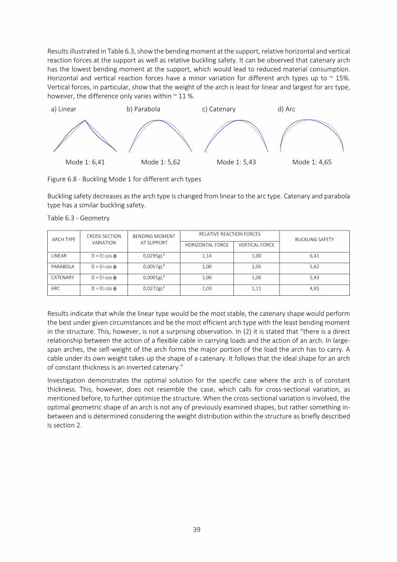
39

Results illustrated in Table 6.3, show the bending moment at the support, relative horizontal and vertical reaction forces at the support as well as relative buckling safety. It can be observed that catenary arch has the lowest bending moment at the support, which would lead to reduced material consumption. Horizontal and vertical reaction forces have a minor variation for different arch types up to ~ 15%. Vertical forces, in particular, show that the weight of the arch is least for linear and largest for arc type, however, the difference only varies within ~ 11 %.

a) Linear b) Parabola c) Catenary d) Arc

Mode 1: 6,41 Mode 1: 5,62 Mode 1: 5,43 Mode 1: 4,65

Figure 6.8 - Buckling Mode 1 for different arch types

Buckling safety decreases as the arch type is changed from linear to the arc type. Catenary and parabola type has a similar buckling safety.

Table 6.3 - Geometry

ARCH TYPE CROSS-SECTION

VARIATION BENDING MOMENT

AT SUPPORT RELATIVE REACTION FORCES

BUCKLING SAFETY HORIZONTAL FORCE VERTICAL FORCE

LINEAR D = EI cos φ 0,0295gL² 1,14 1,00 6,41

PARABOLA D = EI cos φ 0,0057gL² 1,00 1,05 5,62

CATENARY D = EI cos φ 0,0001gL² 1,00 1,06 5,43

ARC D = EI cos φ 0,0272gL² 1,03 1,11 4,65

Results indicate that while the linear type would be the most stable, the catenary shape would perform the best under given circumstances and be the most efficient arch type with the least bending moment in the structure. This, however, is not a surprising observation. In (2) it is stated that “there is a direct relationship between the action of a flexible cable in carrying loads and the action of an arch. In large-span arches, the self-weight of the arch forms the major portion of the load the arch has to carry. A cable under its own weight takes up the shape of a catenary. It follows that the ideal shape for an arch of constant thickness is an inverted catenary.”

Investigation demonstrates the optimal solution for the specific case where the arch is of constant thickness. This, however, does not resemble the case, which calls for cross-sectional variation, as mentioned before, to further optimize the structure. When the cross-sectional variation is involved, the optimal geometric shape of an arch is not any of previously examined shapes, but rather something in-between and is determined considering the weight distribution within the structure as briefly described is section 2.

40

6.2 Arch shape and characteristics

The arch shape is designed having the following input variables:

Overall dimension (centerline)

• Span (𝐿) 𝐿 = 300 𝑚

• Rise (𝑓) 𝑓 = 400 𝑚

• Span/Rise (𝐿/𝑓) 𝐿/𝑓 = 0.75

Box cross-section at crown

• Height (ℎ) ℎ = 2 𝑚

• Width (𝑏) 𝑏 = 2 𝑚

• Thickness (𝑡) 𝑡 = 0.4 𝑚

Box cross-section at base

• Height (ℎ) ℎ = 6 𝑚

• Width (𝑏) 𝑏 = 6 𝑚

• Thickness (𝑡) 𝑡 = 0.4 𝑚

Material Properties

• CONCRETE C90/95

• Elastic Modulus 𝐸 = 44 𝐺𝑃𝑎

• Shear Modulus 𝐺 = 18.3 𝐺𝑃𝑎

• Poison’s Ratio 𝑢 = 0.2

• Thermal exp. Coef. 𝛼 = 1𝐸 − 5

• Weight 𝑤 = 24.9926 𝑘𝑁/𝑚3

The results show that the shape of the arch calculated using the numerical method described in Section 2.2.2, is rather different from any of the previously described analytical functions in section 2.2, equations ( 2-2 ), ( 2-3 ) and ( 2-4 ). In Figure 6.9 it is clearly evident that the arch shape acquired using numerical iterative procedure differs quite significantly, thus indicating that describing an arch shape with mathematical function is a challenging task and require an in-depth understanding.

The function of the flattened catenary is implemented according to the formulations that were used for describing the shape of the Gateway Arch, the contestants used in ( 2-4 ) are described in (4). It is, however, evident that the shape of the Gateway Arch has been governed more by architectural reasons than the mathematical expression of the theoretically ideal shape.

Further, each shape has been evaluated using FEM Software SAP2000, where the structure is subjected to its own self-weight.

Figure 6.9 - Arch shape comparison (centrelines)

0

50

100

150

200

250

300

350

400

450

0 100 200 300

Ris

e, f

Span, L

Numerical Parabola

Catenary Flattened catenary

41

If the bending moment is observed for all of the shapes in Figure 6.10 and Figure 6.11 one can see that the numerically calculated shape gives rise to smallest moments in the structure, as intended.

a) PARABOLA

b) CATENARY

Max/Min Moment 394,13 / -185,77 MNm Max/Min Moment 164,32 / -68,83 MNm

c) FLATTENED CATENARY

d) NUMERICAL

Max/Min Moment 259,45 / -122,90 MNm Max/Min Moment 15,47 / -4,26 MNm

Figure 6.10 - Bending moment diagrams (Support conditions – Pinned) (Scale 1:10000)

42

Figure 6.11 - Bending moment diagrams for different arch shapes.

Also, if the numerical shape is examined more closely in Figure 6.12, it is possible to observe that the bending moment are not exactly zero nor negligible. However, it can be shown that by increasing the degree of discretization of the calculation model, the tendency is for bending moments to decrease toward zero for the numerically acquired shape, as can be observed in Figure 6.13, while for the other shapes the change due to the degree of discretization is insignificant, showed in Table 6.4.

This is a direct consequence of using FEM and Numerical calculation procedure, as the arch is modeled using straight elements in between the calculation points, while the ideal arch shape should be a curve. However, one can also observe in Figure 6.12 that although the magnitude of the bending moment decrease when more elements are used, the results does not necessarily have reached complete convergence. The reason for these discrepancies lies in the numerical calculation method itself, described in Section 2.2.2, where it is emphasized that the method utilizes numerical integration methods in the calculation procedure, which is also an approximation of the real solution. Therefore, in order to further increase the accuracy of the results, by further reducing the bending moment in the structure, it is necessary to adjust the numerical method by implementing more accurate numerical integration methods.

Figure 6.12 - Bending moment diagrams for numerically calculated arch shape for different degrees of discretization.

-200

-100

0

100

200

300

400

0.00 0.10 0.20 0.30 0.40 0.50 0.60 0.70 0.80 0.90 1.00

Ben

din

g M

om

ent

[MN

m]

Coordinate along the arch

PAR CAT FLC NUM

-5

0

5

10

15

0.00 0.10 0.20 0.30 0.40 0.50 0.60 0.70 0.80 0.90 1.00

Ben

din

g M

om

ent

[MN

m]

Coordinate along the arch

NUM_100 NUM_300 NUM_600 NUM_1200

43

Based on the results, presented above, it showed that the numerical method is the most efficient and, therefore, is to be used for determination of arch shape for the prototype building. Also, the degree of discretization to be used in the prototype building is best if 1200 elements are to be used. Although it does not give completely convergent results, it provides reasonable results. The practical implementation of the finite element model, however, is rather demanding if such a large number of elements is used.

Figure 6.13 - Max/Min Bending moment in the numerically calculated arch shape for different degrees of discretization.

In Table 6.4 and Figure 6.14 it is also possible to observe that the horizontal reaction force from FEM analysis and numerical calculation converge as the degree of discretization is increased.

Table 6.4 - Bending moment and reaction forces for different arch shapes and degrees of discretization.

SHAPE

MOMENT [MNm] REACTIONS [MN]

Figure 6.14 - Horizontal reaction force for different degrees of discretization.

DISCR. MAX MIN Fx

(FEM) Fy

(FEM) Fx

(Calc.)

PARABOLA

100 394,13 -185,77 6,87 61,25 -

300 393,94 -185,62 6,86 61,25 -

600 - - - - -

CATENARY

100 164,32 -68,83 5,41 61,58 -

300 164,00 -68,67 5,41 61,58 -

600 - - - - -

FLATTENED CATENARY

100 259,45 -122,90 6,07 61,38 -

300 259,33 -122,75 6,07 61,38 -

600 - - - - -

NUMERICAL

100 15,47 -4,26 4,52 61,91 4,10

300 5,59 -1,55 4,49 61,90 4,34

600 2,87 -0,79 4,48 61,90 4,41

1200 1,46 - 0,39 4,48 61,90 4,44

APP. 1,46 - 0,70 4,48 61,90 -

-5

0

5

10

15

0 200 400 600 800 1000 1200Ben

din

g M

om

ent

[MN

m]

Number of elements

MAX MIN

4

4.1

4.2

4.3

4.4

4.5

4.6

0 200 400 600 800 1000 1200

Rea

ctio

n F

orc

e Fx

[M

N]

Number of elements

Fx (FEM) Fx (Calc.)

44

Table 6.4 also includes an approximate discretization for numerical solution. This type is based on the dense 1200 discretization, where only coordinates matching floor height of every 5 m are extracted and used. Figure 6.15 shows the comparison between the two in terms of bending moment distribution. Bending moment and other forces in the structure are listed in Table 6.4. It is possible to deduct that the results are relatively similar for the two cases and the differences are minor, while the number of finite elements used in the FEM model is reduced significantly to 164 elements, compared to 1200 elements used initially.

This type of discretization allows for “lighter” and more functional FEM model. These characteristics are the main motivation for choosing this discretization for further analysis, as the complexity of the FEM model is expected to increase when extending the analysis to 3-dimensional space. Other vital aspects that would benefit from this type of approximation, are construction considerations, as it would be much easier to construct and erect straight structural elements.

Figure 6.15 - Approximate discretization

-1

-0.5

0

0.5

1

1.5

2

0 0.1 0.2 0.3 0.4 0.5 0.6 0.7 0.8 0.9 1

Ben

din

g M

om

ent

[MN

m]

Coordinate along the arch

NUM_1200 NUM_APP_164

45

The location of the outer and inner mega tubes of the arch can be modeled using few different approaches. The two considered in this study are – modeling inner and outer mega tube to follow an individual funicular line for each tube, further referred to as IND approach, or modeling inner and outer mega tube to perform as a unit and follow one combined funicular line, further referred to as KAS approach. The shape of the arch for the two approaches are slightly different as can be observed in Figure 6.17 and Figure 6.16.

Figure 6.16 shows the IND approach where the location of the inner and outer mega tube is calculated by defining a funicular line for each tube separately. The parameters used in this process to achieve the desired shape are the distance between the mega tubes at the springing and at the crown, respectively 30.0 m and 10.0 m.

Figure 6.16 - Mega tube location

0

50

100

150

200

250

300

350

400

450

-50 0 50 100 150 200 250 300 350

Ris

e [m

]

Span [m]

46

Figure 6.17 shows the KAS approach where the location of the inner and outer mega tube is calculated by defining a funicular line that is the centerline for both mega tubes and by using Kasarnowsky variation in ( 2-14 ) and ( 2-15 ) and varying the distance to the centerline.

In Figure 6.17 it is visually possible to observe that the distance between the mega tubes is decreasing from springing to the crown. In this way manipulating the moment of inertia of the structure to be consistent with the envisioned stiffness variation. The parameters used in this process to achieve the desired variation are the distance between the mega tubes at the springing and at the crown, respectively 30.0 m and 8.926 m. This approach, however, requires a system that connects the mega tubes to evenly distribute the forces, even for the self-weight of the structure. Clearly, more material is expected to be used to design such a system.

Figure 6.17 - Mega tube location with respect to centre-line

0

50

100

150

200

250

300

350

400

450

-50 0 50 100 150 200 250 300 350

Ris

e [m

]

Span [m]

47

Both approaches, however, follow the same cross-sectional linear variation with height. Figure 6.18 illustrates the variation, where one can observe that the cross-section at the bottom of the structure is 3.5 times larger than that of the crown. For IND approach this is valid for each individual mega tube, while for the KAS approach this is valid for the centre-line of the structure, where both mega tubes are considered.

Figure 6.18 - Cross-section area variation along the height of the arch.

Due to the differences between the two approaches, the self-weight of the mega tubes in the structure is slightly different as well.

0.00

0.10

0.20

0.30

0.40

0.50

0.60

0.70

0.80

0.90

1.00

0.00 0.50 1.00 1.50 2.00 2.50 3.00 3.50 4.00

y/f

A(x)/A0

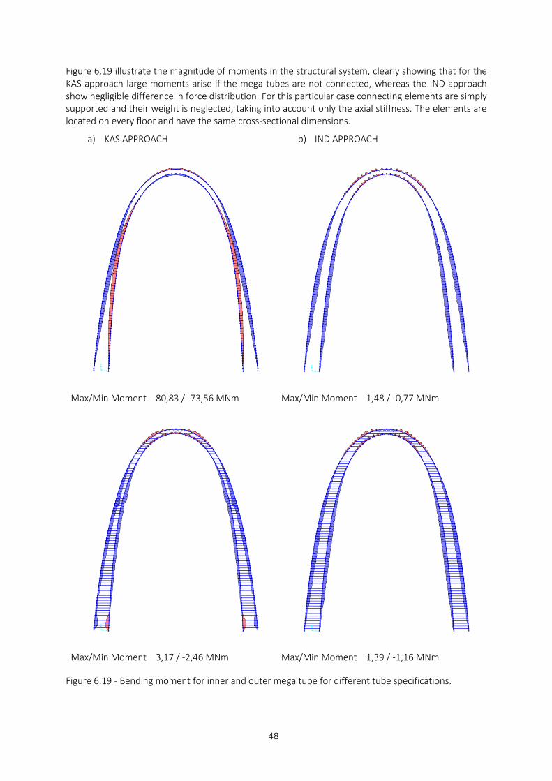
48

Figure 6.19 illustrate the magnitude of moments in the structural system, clearly showing that for the KAS approach large moments arise if the mega tubes are not connected, whereas the IND approach show negligible difference in force distribution. For this particular case connecting elements are simply supported and their weight is neglected, taking into account only the axial stiffness. The elements are located on every floor and have the same cross-sectional dimensions.

a) KAS APPROACH b) IND APPROACH

Max/Min Moment 80,83 / -73,56 MNm Max/Min Moment 1,48 / -0,77 MNm

Max/Min Moment 3,17 / -2,46 MNm Max/Min Moment 1,39 / -1,16 MNm

Figure 6.19 - Bending moment for inner and outer mega tube for different tube specifications.

49

Figure 6.20 also indicates the magnitude of axial forces in the elements connecting the mega tubes. It is possible to observe that, in general, the elements are more axially utilized in the KAS approach, while IND approach rises considerably smaller forces in these elements. If the axial forces are somewhat similar towards the top of the building, then larger differences are noticeable throughout the rest of the structure. This behavior is expected and is a direct consequence of the approach taken in the calculations process for mega tube location. The extra forces in the system are not beneficial and also the results clearly indicate that the IND approach is better of the two, and therefore, is to be used further in the study.

c) KAS APPROACH d) IND APPROACH

Max/Min Axial Force 179,13 / -159,60 kN Max/Min Axial Force 34,32 / -141,75 kN

Figure 6.20 – Axial force distribution in connection elements for different tube specifications.

50

6.3 Bracing system evaluation

Bracing system evaluation is performed by comparison of three different bracing system types, which include some of the most common principles for typical bracing systems. X-BRACING system consist of common steel braces arranged in cross formation, F-BRACING utilizes the principles of steel moment frames, and B-BRACING includes steel truss principles at certain heights along the building. All systems are modeled to have similar weight. For the very top part of the building, above 390 m, the structural element arrangement is kept the same for all three cases. Also, all of the cases include simply supported HE1000B floor beams at every floor level.

Material Properties - Bracing

• STEEL S355

• Elastic Modulus 𝐸 = 210 𝐺𝑃𝑎

• Shear Modulus 𝐺 = 80.7 𝐺𝑃𝑎

• Poison’s Ratio 𝑢 = 0.3

• Thermal exp. Coef. 𝛼 = 1.17𝐸 − 5

• Weight 𝑤 = 76.9 𝑘𝑁/𝑚3

X-BRACING systems have the following parameters:

Steel box cross-section

• Height (ℎ) ℎ = 0.500 𝑚

• Width (𝑏) 𝑏 = 0.250 𝑚

• Thickness (𝑡) 𝑡 = 0.025 𝑚

Cross-braces have pinned connection to mega tubes and have fixed connection at intersection points. The bracing system is not connected with floor beams.

a) X - BRACING

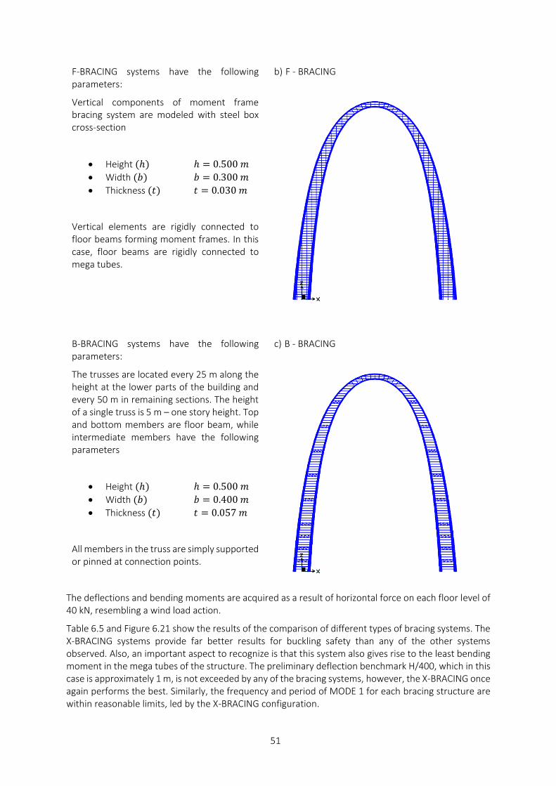
51

F-BRACING systems have the following parameters:

Vertical components of moment frame bracing system are modeled with steel box cross-section

• Height (ℎ) ℎ = 0.500 𝑚

• Width (𝑏) 𝑏 = 0.300 𝑚

• Thickness (𝑡) 𝑡 = 0.030 𝑚

Vertical elements are rigidly connected to floor beams forming moment frames. In this case, floor beams are rigidly connected to mega tubes.

b) F - BRACING

B-BRACING systems have the following parameters:

The trusses are located every 25 m along the height at the lower parts of the building and every 50 m in remaining sections. The height of a single truss is 5 m – one story height. Top and bottom members are floor beam, while intermediate members have the following parameters

• Height (ℎ) ℎ = 0.500 𝑚

• Width (𝑏) 𝑏 = 0.400 𝑚

• Thickness (𝑡) 𝑡 = 0.057 𝑚

All members in the truss are simply supported or pinned at connection points.

c) B - BRACING

The deflections and bending moments are acquired as a result of horizontal force on each floor level of 40 kN, resembling a wind load action.

Table 6.5 and Figure 6.21 show the results of the comparison of different types of bracing systems. The X-BRACING systems provide far better results for buckling safety than any of the other systems observed. Also, an important aspect to recognize is that this system also gives rise to the least bending moment in the mega tubes of the structure. The preliminary deflection benchmark H/400, which in this case is approximately 1 m, is not exceeded by any of the bracing systems, however, the X-BRACING once again performs the best. Similarly, the frequency and period of MODE 1 for each bracing structure are within reasonable limits, led by the X-BRACING configuration.

52

Table 6.5 - Bracing system comparison

TYPE

WEIGHT OF BRACING SYSTEM

MOMENT IN MEGA TUBES [MNm]

DEFLECTION [m] BUCKLING

FACTOR MODAL ANALYSIS (MODE1)

[kN] MAX MIN HORIZONTAL VERTICAL MODE 1 PERIOD [s] FEQUENCY [Hz]

X - BRACING 6009.96 4.19 -4.19 0.219 0.044 30.832 4.948 0.202

F - BRACING 6014.97 18.38 -18.38 0.729 0.087 6.565 9.675 0.103

B - BRACING 6027.49 35.22 -35.22 0.586 0.096 11.720 8.204 0.122

NO - BRACING - 209.67 -209.67 30.869 5.039 0.233 59.571 0.017

Figure 6.21 - Bracing system comparison for Period, Frequency, Buckling Factor and Weight.

0

10

20

30

40

50

60

70

PER

IOD

[s]

X - BRACING F - BRACING

B - BRACING NO - BRACING

0.00

0.05

0.10

0.15

0.20

0.25

FREQ

UEN

CY

[Hz]

X - BRACING F - BRACING

B - BRACING NO - BRACING

0

5

10

15

20

25

30

35

BU

CK

LIN

G F

AC

TOR

X - BRACING F - BRACING

B - BRACING NO - BRACING

0

1000

2000

3000

4000

5000

6000

7000

WEI

GH

T [k

N]

X - BRACING F - BRACING

B - BRACING NO - BRACING

53

6.4 Arch Mega Structure

The results of the analysis concerning 3D arch mega structure shown in Figure 6.22 and described in Section 5 are presented in this section.

Figure 6.22 - Arch Mega Structure

6.4.1 Deformation

Maximum displacement of top occupied story (story 80) for different load cases are listed in Table 6.6

Table 6.6 - Max displacements for story 80

Load case/combination

No P-DELTA P-DELTA

Max displacements Max displacements

mm mm

UX UY UX UY

1 1.4D 0,004 -0,354 0,008 -0,402

2 1.2D + 1.6L -0,098 -0,461 -0,102 -0,524

3 1.2D + 1.0L -0,06 -0,402 -0,061 -0,457

4 1.2D + 0.5W 295,718 582,904 317,88 673,494

5 1.2D + 1.0W + 1.0L 591,369 1166,014 635,686 1347,221

6 0.9D + 1.0W 591,431 1166,188 635,752 1347,419

7 1.0D + 0.5L + 1.0W 425,93 839,774 457,85 970,281

54

It is evident that the wind load is causing the largest lateral deformation, while the self-weight and live load only account for nearly negligible contribution. The results show that it has been possible through the thorough design of the shape of the arch achieve minor deformation due to self-weight of the structure, as intended. Furthermore, it can be observed that the structure undergoes larger deformations in the y-direction (out-of-plane of the arch) while being a lot more robust against deformations in the x-direction (in-plane of the arch). Evidently, it is apparent that the lateral forces would govern the design of the structure, which corresponds to the general idea of the lateral load being the most critical for high-rise structures. Important lateral loads, that have not been included in this study comes from the actions of earthquakes and, therefore, must be considered, if relevant, in further analysis of this structure.

It can also be observed that P-Delta effects cause differences in the deformation magnitude of approximately 7 % in the x-direction and 13.5 % in the y-direction, suggesting that if the stiffness of the structure is higher, the structure is subjected to lower influence from P-Delta effects on the deformation of the structure.

Figure 6.23 and Figure 6.24 show the displacements for service limit wind loads considering P-Delta effects in the x-direction and y-direction, respectively. Similarly, P-Delta effects can be observed having a greater effect in the y-direction than x-direction. Figure 6.25 illustrates the displacements in two principal directions shown in Figure 6.23 and Figure 6.24.

Figure 6.23 - Displacements for service limit wind loads considering P-delta effects.

0

10

20

30

40

50

60

70

80

0 100 200 300 400 500 600

Sto

ry

Displacement x-direc. [mm]

PDELTA No PDELTA

55

Figure 6.24 - Displacements for service limit wind loads considering P-delta effects.

Figure 6.25 - Displacements for service limit wind loads in two principal directions – x and y.

0

10

20

30

40

50

60

70

80

0 200 400 600 800 1000 1200

Sto

ry

Displacement y-direc. [mm]

PDELTA No PDELTA

56

6.4.2 Story drift

In Figure 6.26 it is possible to observe the story drift ratios of the building under service limit state wind loads. The story drift ratios are defined as the differences of horizontal displacements between two consecutive stories divided by the floor heights, ∆u/hfloor, and are determined in ETABS.

According to the ASCE 7-10 code, the maximum story drift ratio is recommended to be limited between 1/400 and 1/600 for service limit state verifications. Figure 6.26 shows that the maximum story drift ratio of the arch mega structure exceeds the limit of 1/600 but doesn’t exceed the lower limit, which is 1/400 in the x-direction (in-plane of the arch), however, in y-direction (out-of-plane of the arch) the structure has higher story drift ratios exceeding the limit of 1/600 and reaching up to 1/250 at peak. Clearly, these results show the difference between the natures of story drifts through the structure in the two principal directions. Also, it is evident that these results would not be satisfactory for the design verification purposes, however, the results are indicative that structure is not entirely out of proportion and it is expected that the bracing of the structure could be improved to perform adequately, satisfying story drift requirements.

Wind SLS Max

Wind SLS Max

Figure 6.26 – Max story drift ratios for service limit wind loads.

0

10

20

30

40

50

60

70

80

0 0.001 0.002 0.003

Sto

ry

Story drift ratio x-direc.

No PDELTA PDELTA

1/400 1/600

0

10

20

30

40

50

60

70

80

0 0.002 0.004 0.006

Sto

ry

Story drift ratio y-direc.

No PDELTA PDELTA

1/250 1/600

57

6.4.3 Mode shapes and frequencies

Table 6.7 shows the first twelve natural frequencies, periods and vibration modes for the arch mega structure, both with and without P-delta effects. Annex E shows the first 12 vibration modes in figures.

Table 6.7 - Modal Periods and Frequencies

Mode Vibration Mode

No P-DELTA P-DELTA

Period Frequency Period Frequency

sec Hz sec Hz

1 y-axis bending 9,725 0,103 10,432 0,096

2 Asymmetrical x-axis bending 6,849 0,146 7,103 0,141

3 Torsion + Asymmetrical x-axis bending 5,155 0,194 5,408 0,185

4 Symmetrical x-axis bending 2,967 0,337 3,021 0,331

5 Torsion + Symmetrical x-axis bending 2,499 0,400 2,567 0,390

6 Asymmetrical x-axis bending 1,803 0,555 1,829 0,547

7 Torsion + Asymmetrical x-axis bending 1,674 0,597 1,699 0,588

8 Torsion + Symmetrical x-axis bending 1,285 0,778 1,317 0,759

9 Symmetrical x-axis bending 1,228 0,815 1,246 0,803

10 Torsion + Asymmetrical x-axis bending 1,135 0,881 1,166 0,857

11 Torsion + Symmetrical x-axis bending 1,011 0,990 1,027 0,973

12 Asymmetrical x-axis bending 0,931 1,074 0,975 1,026

In Table 6.7 it can be observed that the natural frequency of first vibration mode is 0.103 Hz, which is slightly lower than that of the second mode at 0.146 Hz, suggesting that the structure has lower stiffness in y-direction or the out-of-plane direction of the arch. This type of behavior of the structure is generally expected and can be designed to have a better response if necessary. To give a perspective of the response of the structure, it is possible to note the response of other high-rise buildings in the world. The Shanghai Center has a fundamental frequency of 0.1105 Hz while the total height is 632 m (9). The Ping An Finance Center has a fundamental frequency of 0.116 Hz (9) while the total height is 660m (structural height 588m). It is rather difficult to directly compare structures with vastly different structural shape and system, but a good indication of the structural response of the arch mega structure relative to iconic high-rise buildings can be drawn. Although the height of the arch mega structure is listed at 405 m high, the centerline of the structure reaches approximately 900 m, making it difficult to compare the structure to more conventional shaped high-rise buildings. On the other hand, the results are acquired through analysis consisting of many assumptions and simplifications, therefore, interpretation of the results only serve the purpose of indicative nature, however, it is evident that tube mega frame structural system has a relatively high stiffness, especially in the x-direction. Also, at this time, it is not known and is very unlikely, that any of the more conventional structural systems could be adapted to support a structure of this particular shape with higher efficiency.

When P-delta effects are considered, it can be observed that the fundamental period of the structure increases from 9.725s to 10.432s, which is approximately 6.8% larger in the y-direction, while in the x-direction the fundamental period of the structure increases from 6.849s to 7.103s, which is approximately only 3.6% larger. This suggests that the stiffness of the structure is reduced by the P-Delta effects, however, the magnitude of the effect of P-Delta effects are different in the two principal directions.

58

Figure 6.27 and Figure 6.28 visualize the difference when P-Delta effects are considered. It can be observed that the increase of the period of the structure reduces for every consecutive vibration mode, and the differences are nearly negligible for the higher modes, however, the decrease in the frequency of the structure due to P-Delta, is relatively constant for every consecutive vibration mode, and the differences are nearly negligible, which generally suggest that the stiffness of the structure is reduced due to the P-Delta effects.

Figure 6.27 - Modal Periods

Figure 6.28 - Modal Frequencies

0

1

2

3

4

5

6

7

8

9

10

11

1 2 3 4 5 6 7 8 9 10 11 12

Per

iod

[s]

Mode

No P-DELTA P-DELTA

0.00

0.10

0.20

0.30

0.40

0.50

0.60

0.70

0.80

0.90

1.00

1.10

1.20

1 2 3 4 5 6 7 8 9 10 11 12

Freq

uen

cy [

Hz]

Mode

No P-DELTA P-DELTA

59

6.4.4 Reaction forces

Figure 6.29 shows the magnitude of the reaction forces for different load combination described in section 5.4. The support numbering is consistent with Figure 5.4 in section 5.5. It can be observed that the structure is not subjected to uplifting forces under the specific loading conditions, eliminating the need for more complex foundation design. Also, for load combination LC1 to LC3, the symmetric nature of the structure can be observed, as the magnitude of the vertical loads is equal for supports symmetrical around x and y symmetry axis.

Figure 6.29 - Vertical reaction forces for different load combinations.

Figure 6.30 shows the differences in vertical reaction forces due to P-Delta effect for different load combinations. It can be observed that the differences are nearly negligible for a case which consider vertical loads, while for combinations including lateral loads, the p-delta effects account for up to 10 MN of the vertical reaction force.

Figure 6.30 - Differences in vertical reaction forces due to P-Delta effect for different load combinations.

0

50

100

150

200

250

300

350

400

LC1 LC2 LC3 LC4 Max LC4 Min LC5 Max LC5 Min LC6 Max LC6 Min LC7 Max LC7 Min

Rea

ctio

n F

orc

e [M

N]

1 46 284 329 655 700 938 983

-15

-10

-5

0

5

10

15

LC1 LC2 LC3 LC4 Max LC4 Min LC5 Max LC5 Min LC6 Max LC6 Min LC7 Max LC7 Min

Rea

ctio

n F

orc

e d

iffe

ren

ce [

MN

]

1 46 284 329 655 700 938 983

60

6.4.5 Buckling

The buckling analysis for the self-weight of the structure did not provide tangible results for the purpose of this study. The analysis resulted in capturing local buckling modes of the braces in the structural system as these buckling modes proved to have much smaller buckling safety than that of the whole structure itself, therefore the intent of observing global buckling modes was not fulfilled. The suspected difficulties capturing global buckling of the structure, most likely occur due to the very basic application of the self-weight in the finite element analysis. Since all load is applied in one step, large axial forces arise in bracing elements due to initial deformation of the structure. These forces are expected to be reduced if more accurate load application is used, employing quality construction sequence analysis. On the other hand, the results showed the buckling factors to be higher than 1 for all modes determined, suggesting that the structural safety due to buckling would not be of concern for the global buckling modes as well.

61

7 Conclusion

The aim of this thesis is the evaluation of the structural performance of tube mega frame structural system in arch shape buildings. The evaluation of high-rise structures requires multipart analysis including various phases and degrees of complexity in order to demonstrate the adequacy of the structural system to be built and perform according to all of the rules and regulations. The ultimate confirmation of the structural system is the actual construction and exploitation of a building as monitoring of the structure allow for verification and if necessary calibration of the calculation models. When the structural system has not been built, the analysis relies on the physical knowledge of the structural principles, as in the case of an arch mega structure that has been examined in this thesis. Nonetheless, the simplified models of the arch mega structure provide a generalized idea of the behavior of the structural system and globally show that the tube mega frame structural system potentially can be adopted and demonstrate the feasible and efficient performance of the structural system for arch shaped high-rise buildings. Also, this thesis account only for few initial phases in the analysis of such novel high-rise structure and is based on multiple limitations and assumptions, however, the results presented in this study should provide the basis to build upon on studying equivalent structures.

Through the study, it has been possible to demonstrate that the arch shape can be designed to transfer a specific load in very efficient way. The arch is most effective when designed for self-weight of the structure. The more precisely the load is accounted for the more efficient the structure would perform. The tools used for determination of the arch shape exhibit good accuracy, however, some improvements would be beneficial. The numerical procedure discretizes the structure along the horizontal axis. While this approach is effective for bridge structures with large span to rise ratios, for a structure with low span to rise ratios this approach is not very practical as a large number of elements are required to achieve convergent results. Also, numerical integration methods could be improved for better results.

The bracing system evaluation provides only indicative results of potentially favoring bracing system out of a few options. Although the results show that the bracing system has good properties for increasing the overall stiffness of the structure, it is expected that large improvements can be achieved in this area. It is often that combinations of different bracing systems are used for high-rise structures to improve the performance.

The results of the analysis of arch mega structure in ETABS demonstrate that the tube mega frame structural system has high in-plane arch stiffness, while out-of-plane stiffness is comparatively lower. These results are not unexpected, as a thorough evaluation of the bracing system for out-of-plane stiffness is not presented in this thesis. Nonetheless, the provided results show that structural system under consideration is within reasonable limits and prone to significant improvements. The P-Delta effects have a non-negligible impact on the structure and should be included in the analysis. The differences due to P-Delta range from 5% to 13%, depending on specific parameter under consideration. On few occasions, the tendency of P-delta effects having a smaller impact on stiffer parts of the structure was noted.

The application of the self-weight in the finite element model does not follow the most accurate principles. For structures of such magnitude construction sequence analysis is preferred. The consequences of not implementing construction sequence are evident throughout the results. Larger deformation and excessive forces occur in structural elements that would otherwise not suffer from such effects under self-weigh. The elements of the bracing system are particularity exposed to this flaw in the analysis process.

62

The results provide enough evidence to that the tube mega frame structural system can be used and have adequate design and performance when implemented in arch shaped buildings. Also, at this time, it is not known and is very unlikely, that any of the more conventional structural systems could be adapted to support a structure of this particular shape with higher efficiency.

63

8 Further studies

Further studies built upon this thesis can be led in various directions to advance the understanding of the structural system of tube mega frame in arch shaped buildings. Evidently, more accurate modeling and evaluation of the material properties including nonlinear properties would be recommended, thus such phenomena as shrinkage and creep could be accounted for in concrete elements and yielding in steel elements. Also, a thorough study of the bracing system could be undertaken to improve the effectiveness of the system and also examine the connection more closely. The foundation for such structure are of utmost importance and should be studied in-depth, providing more insight on the type of support conditions that should be used in finite element analysis. The structure should also be examined using all of the required loads in relevant design codes, including seismic actions, if necessary, as these actions might reveal flaws or weaknesses in the structural system, that should be addressed.

An important aspect that should be comprehensively studied is the construction process and sequence of this structure. Understanding the construction process could provide indications of the economic feasibility of the structure as well as give a better understanding of how to model the structure so that the application of the self-weight is done as accurately as possible and temporary supporting conditions of the structure are fully understood.

Another interesting investigation might include a study of the possible use of influence lines. One suggestion might be, that since the structure is related to slanted elevator technologies, it would be curious to see how their movement might influence the various arch structures under investigation.

These suggestions are just a few among many possibilities of studying this particular structure. Further studies are vital in order to increase the understanding and knowledge of these type of structures so that it would be possible realize such buildings in real life.

64

65

9 References

1. Sundquist, Håkan. Arch Structures. Stockholm : KTH Structural Design & Bridges, 2010. ISSN 1103-4289.

2. T.H.G., Megson. Chapter 6 - Arches, In Structural and Stress Analysis (2) Pages 133-149. Oxford : Butterworth-Heinemann, 2005. ISBN 9780750662215.

3. How the Gateway Arch Got its Shape. Osserman, Robert. Nexus Network Journal No. 2, s.l. : © 2010 Kim Williams Books, Turin, 2010, Vol. 12. DOI 10.1007/s00004-010-0030-8.

4. Mathematics of the Gateway Arch. Osserman, Robert. Number 2, s.l. : Notices of the AMS, 2010, Vol. 57. ISSN 0002-9920.

5. Routh, Edward John. A TREATISE ON ANALYTICAL STATICS WITH NUMEROUS EXAMPLES. Second Edition. Cambridge : CAMBRIDGE UNIVERSITY PRESS , 1909. Vol. Volume 1.

6. CTBUH. Criteria for the Defining and Measuring of Tall Buildings. Chicago, IL, USA : Council on Tall Buildings and Urban Habitat, 2016.

7. —. CTBUH Year in Review: Tall Trends of 2016. Chicago, IL 60603 USA : The Council on Tall Buildings and Urban Habitat, 2016.

8. Partovi, Arezo and Svärd, Jenny. Global Analysis of tall buildings with tubed mega frame structures. Stockholm : ISRN KTH/BKN/EX--489--SE, 2016. ISSN 1103-4297.

9. Zhang, Han. Global Analysis and Structural Performance of the Tubed Mega Frame. Stockholm : ISRN KTH/BKN/EX--426--SE, 2014. ISSN 1103-4297.

10. Cook, Robert David. Concepts and Applications of Finite Element Analysis, 4th Ed. University of Wisconsin-Madison : John Wiley & Sons, Inc., 2002. ISBN: 978-0-471-35605-9.

11. Bathe, Klaus Jurgen and Wilson, Edward L. NUMERICAL METHODS IN FINITE ELEMENT ANALYSIS. New Jersey : PRENTICE-HALL, INC., 1976.

12. Computers & Structures, Inc. CSI Analysis Reference Manual. Berkeley, California, USA : Computers & Structures, Inc., 2016. ISO# GEN062708M1 Rev.15.

13. —. Lateral Loads Manual. Berkeley, California, USA : Computers & Structures, Inc., 2016. ISO ETA122815M4 Rev. 1.

14. Hallebrand, Erik and Jacobsson, Wilhelm. STRUCTURAL DESIGN OF HIGH-RISE BUILDINGS. Lund : Printed by Media-Tryck LU, 2016. ISSN 0281-6679.

15. Rombach, Guenter Axel. Finite-element design of concrete structures, Practical problems and their solutions. London : ICE Publishing, 2011. Vol. Second edition.

66

67

10 Annex

10.1 Annex A

Among the most common are linear, arc, catenary and parabola. Each of these shapes has a different performance with respect to the forces that arise in the structure when external loads are applied. To get an idea of how these geometrically different arches behave, a brief evaluation is performed using Finite Element Method in software SAP2000.

a) Linear b) Parabola c) Catenary d) Arc

Figure 10.1 – Geometry of different arch types

The geometry in these examples is based on well-established functions for respective shapes. To make a comparison the span and the raise are kept constant with span to raise the ratio of 2:1, which allows for the establishment of three points that these arches will pass through, therefore allowing for straightforward derivation of required constants for the functions describing arch shape:

𝑝1 = (𝑥1, 𝑦1) = (0,0) ; 𝑝2 = (𝑥2, 𝑦2) = (225,225) ; 𝑝3 = (𝑥3, 𝑦3) = (450,0)

Based on these input values it is possible to establish constants in respective functions:

LINEAR

𝑓(𝑥) = 𝑎𝑥 + 𝑏

𝑓(𝑥) = 1,0𝑥2 𝑓𝑜𝑟 0 < 𝑥 < 225

𝑓(𝑥) = −1,0𝑥2 + 450 𝑓𝑜𝑟 0 < 𝑥 < 450

PARABOLIC

𝑓(𝑥) = 𝑎𝑥2 + 𝑏𝑥 + 𝑐

𝑓(𝑥) = −1

225𝑥2 + 2𝑥 𝑓𝑜𝑟 0 < 𝑥 < 450

CATENARY

𝑓(𝑥) = 𝑦0 − 𝑎 ∙ (cosh (𝑥 − 𝑥0

𝑎) − 1) , 𝑤ℎ𝑒𝑟𝑒 (𝑥0, 𝑦0) 𝑐𝑜𝑜𝑟𝑑𝑖𝑛𝑎𝑡𝑒 𝑜𝑓 𝑎𝑝𝑒𝑥

𝑓(𝑥) = 225 − 139,2208 ∙ (cosh (𝑥 − 225

139,2208) − 1) 𝑓𝑜𝑟 0 < 𝑥 < 450

ARC

𝑥2 + 𝑦2 + 𝐴𝑥 + 𝐵𝑦 + 𝐶 = 0

𝑓(𝑥) = √450 ∙ 𝑥 − 𝑥2 𝑓𝑜𝑟 0 < 𝑥 < 450

The cross-sectional variation is set to be the same for all arch types at the crown and varying towards the springing based on the angle φ. The structure is analyzed under the load of a self-weight g, by keeping the span to raise ratio constant.

68

10.2 Annex C

Funicular.m

clear, clc, close all

% INPUT f = 405; % Arch rise [m] L = 330; % Arch span [m] hb = 6; % Mega tube height at bottom [m] ht = 2; % Mega tube height at top [m] t = 0.4; % Mega tube thickness [m] E = 44000000; % Elastic modulus w = -24.9926; % Weight of concrete [kN/m³] n1 = 1200; % Discretization dx = L/n1; % Element length [m] u = (0:dx/(L/2):1)'; % u-coordinates x = (0:dx:L)'; % x-coordinates yin=(-(4*f/L^2)*((u*L/2)-L/2).^2+f)/f; % Initial guess y-coordinates err = 1; % Initiate error value iter = 1; % Initiate itteration value

% Iterative procedure to determine ideal arch shape under self-weight while err > 1E-15 [ynor,n,err,Y,Y1,Z,H,A,Qb,coefH] = FunInt(f,L,hb,ht,t,u,yin,dx,n1); yin = ynor; iter = iter + 1; end fprintf('Just finished iteration #%d\n', iter); fprintf('Extimated error %d\n', err);

Hq1 = coefH*(w*A(n,:))*L^2/f; % Horizontal force

% Determine arch mega tube location if Kasarnowsky is used [Dx,Ixx,yx,yex,xex,yin,xin] = Kasarnowsky(x,L,n,t,E,Y,Y1,H,A);

% Calculate common arch shapes with the same overall dimensions [ypar,yflc,ycat,Apar,Aflc,Acat] = SHAPES(f,L,hb,ht,t,n1);

% Plot Results figure plot(x,ypar), hold on plot(x,yflc), hold on plot(x,ycat), hold on plot(x,Y), hold on plot(xex,yex),hold on plot(xin,yin),hold on

figure plot(x,Qb), hold on plot(A,Y), hold on plot(x,A), hold on plot(x/L,Dx/Dx(n,:)), hold on, axis([0 1 0 Dx(1,:)/Dx(n,:)]);

69

SHAPES.m function [ypar,yflc,ycat,Apar,Aflc,Acat] = SHAPES(f,L,hb,ht,t,n1);

% INPUT A1 = (4*(hb*t-t^2)); % Mega tube area at bottom

[m²] A0 = (4*(ht*t-t^2)); % Mega tube area at top [m²] dx = L/n1; % Element length [m] u = (0:dx/(L/2):1)'; % u-coordinates x = (0:dx:L)'; % x-coordinates n = length(u); % u vector size

% Parabolic shape ypar = -4*f/L^2*(x-L/2).^2+f; % y-coord for parabolic shape for i = 1:n hpar(i,:) = hb-(hb-ht)*ypar(i,:)/f; % cross-section height Apar(i,:) = 4*(hpar(i,:)*t-t^2); % cross-section area end Apar = [Apar(1:n-1,:); flipud(Apar)]; % cross-section height hpar = [hpar(1:n-1,:); flipud(hpar)]; % cross-section area

% Catenary shape syms acat t0 = solve(f-acat*(cosh((L/2)/acat)-1),acat); ycat = f-t0*(cosh((x-L/2)/t0)-1); % y-coord for catenary shape for i = 1:n hcat(i,:) = hb-(hb-ht)*ycat(i,:)/f; % cross-section height Acat(i,:) = 4*(hcat(i,:)*t-t^2); % cross-section area end Acat = [Acat(1:n-1,:); flipud(Acat)]; % cross-section area hcat = [hcat(1:n-1,:); flipud(hcat)]; % cross-section height

% Flattened catenary (Gateway Arch) B = 2/L*acosh(A1/A0); yflc = -(f/(A1/A0-1))*(cosh(B*(x-L/2))-1)+f;% y-coord flattened cat.

shape for i = 1:n hflc(i,:) = hb-(hb-ht)*yflc(i,:)/f; % cross-section height Aflc(i,:) = 4*(hflc(i,:)*t-t^2); % cross-section area end Aflc = [Aflc(1:n-1,:); flipud(Aflc)]; % cross-section area hflc = [hflc(1:n-1,:); flipud(hflc)]; % cross-section height

end

FunInt.m function [ynor,n,err,Y,Y1,Z,H,A,Qb,coefH] =

FunInt(f,L,hb,ht,t,u,yin,dx,n1); % Calculation procedure according to "Arch Structures" by H.Sundquist % Chapter 3.3 - Numerical calculation of the funicular line

A1 = 2*(4*(hb*t-t^2)); % Mega tube area at bottom [m²] A0 = 2*(4*(ht*t-t^2)); % Mega tube area at top [m²] q0 = 1; % Unit load initiation n = length(u); % u vector size y1in = zeros(n,1); % Prelocating array

70

h = zeros(n,1); % Prelocating array A = zeros(n,1); % Prelocating array secphi = zeros(n,1); % Prelocating array qb = zeros(n,1); % Prelocating array error = zeros(n,1); % Prelocating array err = zeros(n,1); % Prelocating array y1 = zeros(n,1); % Prelocating array y = zeros(n,1); % Prelocating array for i = 1:n if i==1 y1in(i,:) = 1/(2*dx)*(-3*yin(i,:)+4*yin(i+1,:)-yin(i+2,:))*f; elseif i==n y1in(i,:) = 0; else y1in(i,:) = 1/(2*dx)*(yin(i+1,:)-yin(i-1,:))*f; end h(i,:) = hb-(hb-ht)*yin(i,:); A(i,:) = 2*4*(h(i,:)*t-t^2); secphi(i,:) = sec(atan(y1in(i,:))); qb(i,:) = q0*A(i,:)/A0*secphi(i,:); end

for i = 1:n-1 if i==n y1(n,:) = 0; elseif i == n-1 y1(n-1,:) = qb(n,:)/2; else y1(n-(i+1),:) = trapz(qb(n-i:n,:)); % trapezoidal integration end end

for i = 1:n if i == 1 y(i,:) = 0; else y(i,:) = trapz(y1(1:i,:)); % trapezoidal integration end end

ynor = y./max(y); for i = 1:n error(i) = abs(1-abs((ynor(i)/yin(i)))); end err = max(error); yin = ynor; coefH = y(n,:)/(n1*n1);

Y = [ynor(1:n-1,:)*f; flipud(ynor*f)]; % y-coord for funicular Y1 = [y1in(1:n-1,:); -flipud(y1in)]; % Slope Z = 20*((f-Y)/f).^2+30; % Define final equation H = [h(1:n-1,:); flipud(h)]; % Height of cross-section A = [A(1:n-1,:); flipud(A)]; % Area of cross-section Qb = [qb(1:n-1,:); flipud(qb)]; % Projected weight of arch end

71

Kasarnowsky.m function [Dx,Ixx,yx,yex,xex,yin,xin] = Kasarnowsky(x,L,n,t,E,Y,Y1,H,A)

Ixxb = 2*(H(1,:)^4/12-(H(1,:)-2*t)^4/12+(A(1,:))*15^2); % 2nd Moment of

area Ixxt = 2*(H(n,:)^4/12-(H(n,:)-2*t)^4/12+(A(n,:))*4.463^2);% 2nd Moment of

area D0 = E*Ixxt*cos(0); % Bending Stiffness Da = E*Ixxb*cos(atan(Y1(1,:))); % Bending Stiffness Dx = zeros(length(x),1); % Prelocating array Ixx = zeros(length(x),1); % Prelocating array yx = zeros(length(x),1); % Prelocating array

for i = 1:length(x) if x(i,:) < L/2*(1-(D0/Da)^(1/4)); Dx(i,:) = Da*(1-2*x(i,:)/L)^4; elseif x(i,:)< L-L/2*(1-(D0/Da)^(1/4)); Dx(i,:) = D0; else Dx(i,:) = Da*(1-2*x(i,:)/L)^4; end Ixx(i,:) = Dx(i,:)/(E*cos(atan(Y1(i,:)))); yx(i,:) = sqrt((Ixx(i,:)/2-(H(i,:)^4-(H(i,:)-2*t)^4)/12)/(A(i,:))); end

yex = zeros(n,1); % Prelocating array xex = zeros(n,1); % Prelocating array yin = zeros(n,1); % Prelocating array xin = zeros(n,1); % Prelocating array

for i = 1:length(Y) yex(i,:) = Y(i,:)+sin(pi/2-atan(Y1(i,:)))*yx(i,:); xex(i,:) = x(i,:)-cos(pi/2-atan(Y1(i,:)))*yx(i,:); yin(i,:) = Y(i,:)-sin(pi/2-atan(Y1(i,:)))*yx(i,:); xin(i,:) = x(i,:)+cos(pi/2-atan(Y1(i,:)))*yx(i,:); end end

72

10.3 Annex D

The list is adapted from (1).

Nr. Name Country Max-span Opened Material 1 Chaotianmen China 552 2008 STEEL 2 Lupo Huangpu China 550 2003 STEEL 3 New River Gorge USA 518 1976 STEEL 4 Bayonne Kill van Kull USA 504 1931 STEEL 5 Sidney Harbour Australia 503 1932 STEEL 6 Chenab India 461 2008 STEEL 7 Wushan China 460 2005 STEEL 8 Wanxian China 420 1997 CONCRETE 9 Caiyuanba China 420 2005 STEEL 10 Krk 1 Yugoslavia 390 1977 CONCRETE 11 Fremont USA 383 1973 STEEL 12 Numata River Gorge Japan 380 2007 STEEL 13 Port Mann Canada 366 1964 STEEL 14 Yajisha China 360 2000 STEEL 15 Trois-Rivers Canada 355 1967 STEEL 16 Beppu-Myoban Japan 351 1989 CONCRETE 17 Thatcher Panama 344 1962 STEEL 18 Laviolette Canada 335 1967 STEEL 19 Jiangjiehe China 330 1995 CONCRETE 20 Zdakov Czech Republic 330 1967 STEEL 21 Runcorn-Widnes UK 330 1961 STEEL 22 Birchenough Zimbabwe 329 1935 STEEL 23 Hoover dam Bypass USA 323 2008 CONCRETE 24 Nagasaki-Sasebo Japan 317 1955 STEEL 25 Glen Canyon USA 313 1959 STEEL 26 Yongjiang China 312 1998 CONCRETE 27 Lewiston-Queenston USA 305 1962 STEEL 28 Amizade Brazil 290 1964 CONCRETE 29 Tjörnbro 1 Sweden 288 1960 STEEL 30 Ponte Infante Dom Henrique Portugal 280 2003 CONCRETE 31 Bloukrans South Africa 272 1983 CONCRETE 32 Arrabida, Oporto Portugal 270 1963 CONCRETE 33 Sandöbron Sweden 264 1943 CONCRETE 34 Wilde Gera Germany 252 2000 CONCRETE 35 Femarnsund Germany 248 1963 STEEL 36 Svinesundsbro Norway-Sweden 247 2005 CONCRETE 37 Sibenik Yugoslavia 246 1966 CONCRETE 38 Fiumarello Italy 231 1961 CONCRETE 39 Zaporello Russia 228 1952 CONCRETE 40 Viaur France 220 STEEL 41 Lingenau Austria 210 1968 CONCRETE 42 Västerbron Sweden 204 1935 STEEL 43 Wu China 200 1988 CONCRETE 44 Frederistadsbron Norway 196 STEEL 45 Karmsund Norway 184 1955 STEEL 46 Tranebergsbron Sweden 181 1934 CONCRETE 47 Djuröbron Sweden 180 1962 CONCRETE 48 Wupper Bridge Germany 180 1890 STEEL 49 Eads Bridge USA 158 1874 STEEL 50 Svinesundsbro Norway-Sweden 155 1946 CONCRETE 51 Årstabron Sweden 151 1929 STEEL 52 Tärendo ö Kalix älv Sweden 122 1935 CONCRETE 53 Wuchao China 120 1991 STONE 54 Skanstullsbron Sweden 112 1947 CONCRETE 55 Colossus UK 103 WOOD 56 Anji China 37 600 STONE 57 Coalbrookdale UK 30 1776 STEEL

73

10.4 Annex E

Mode 1: 9.725 s

Mode 2: 6.849 s

Mode 3: 5.155 s

Mode 4: 2.967 s

Mode 5: 2.499 s

Mode 6: 1.803 s

74

Mode 7: 1.674 s

Mode 8: 1.285 s

Mode 9: 1.228 s

Mode 10: 1.135 s

Mode 11: 1.011 s

Mode 12: 0.931 s

TRITA TRITA-BKN Examensarbete 505, Brobyggnad 2017

ISSN ISSN 1103-4297

ISRN ISRN KTH/BKN /EX-505-SE

www.kth.se