Structural control of elastic moduli in ferrogels and the importance of non-affinedeformationsGiorgio Pessot, Peet Cremer, Dmitry Y. Borin, Stefan Odenbach, Hartmut Löwen, and Andreas M. Menzel

Citation: The Journal of Chemical Physics 141, 124904 (2014); doi: 10.1063/1.4896147 View online: http://dx.doi.org/10.1063/1.4896147 View Table of Contents: http://scitation.aip.org/content/aip/journal/jcp/141/12?ver=pdfcov Published by the AIP Publishing Articles you may be interested in Hardening transition in a one-dimensional model for ferrogels J. Chem. Phys. 138, 204906 (2013); 10.1063/1.4807003 Full-field deformation of magnetorheological elastomer under uniform magnetic field Appl. Phys. Lett. 100, 211909 (2012); 10.1063/1.4722789 Measuring the deformation of a ferrogel sphere in a homogeneous magnetic field J. Chem. Phys. 128, 164709 (2008); 10.1063/1.2905212 Control of flow through porous media using polymer gels J. Appl. Phys. 92, 1143 (2002); 10.1063/1.1487454 Magnetically textured - Fe 2 O 3 nanoparticles in a silica gel matrix: Structural and magnetic properties J. Appl. Phys. 83, 7776 (1998); 10.1063/1.367952

This article is copyrighted as indicated in the article. Reuse of AIP content is subject to the terms at: http://scitation.aip.org/termsconditions. Downloaded to IP:

134.99.64.185 On: Fri, 26 Sep 2014 07:37:49

THE JOURNAL OF CHEMICAL PHYSICS 141, 124904 (2014)

Structural control of elastic moduli in ferrogels and the importanceof non-affine deformations

Giorgio Pessot,1 Peet Cremer,1 Dmitry Y. Borin,2 Stefan Odenbach,2 Hartmut Löwen,1

and Andreas M. Menzel1,a)

1Institut für Theoretische Physik II: Weiche Materie, Heinrich-Heine-Universität Düsseldorf,D-40225 Düsseldorf, Germany2Technische Universität Dresden, Institute of Fluid Mechanics, D-01062 Dresden, Germany

(Received 1 July 2014; accepted 9 September 2014; published online 25 September 2014)

One of the central appealing properties of magnetic gels and elastomers is that their elastic modulican reversibly be adjusted from outside by applying magnetic fields. The impact of the internal mag-netic particle distribution on this effect has been outlined and analyzed theoretically. In most cases,however, affine sample deformations are studied and often regular particle arrangements are consid-ered. Here we challenge these two major simplifications by a systematic approach using a minimaldipole-spring model. Starting from different regular lattices, we take into account increasingly ran-domized structures, until we finally investigate an irregular texture taken from a real experimentalsample. On the one hand, we find that the elastic tunability qualitatively depends on the structuralproperties, here in two spatial dimensions. On the other hand, we demonstrate that the assumptionof affine deformations leads to increasingly erroneous results the more realistic the particle distri-bution becomes. Understanding the consequences of the assumptions made in the modeling processis important on our way to support an improved design of these fascinating materials. © 2014 AIPPublishing LLC. [http://dx.doi.org/10.1063/1.4896147]

I. INTRODUCTION

In the search of new materials of outstanding novelproperties, one route is to combine the features of differ-ent compounds into one composite substance.1–5 Ferrogelsand magnetic elastomers provide an excellent example forthis approach. They consist of superparamagnetic or ferro-magnetic particles of nano- or micrometer size embeddedin a crosslinked polymer matrix.6 In this way, they combinethe properties of ferrofluids and magnetorheological fluids7–16

with those of conventional polymers and rubbers:17 we obtainelastic solids, the shape and mechanical properties of whichcan be changed reversibly from outside by applying externalmagnetic fields.6, 18–25

This magneto-mechanical coupling opens the door to amultitude of applications. Deformations induced by exter-nal magnetic fields suggest a use of the materials as softactuators26 or as sensors to detect magnetic fields and fieldgradients.27, 28 The non-invasive tunability of the mechanicalproperties by external magnetic fields makes them candidatesfor the development of novel damping devices29 and vibrationabsorbers19 that adjust to changed environmental conditions.Finally, local heating due to hysteretic remagnetization lossesin an alternating external magnetic field can be achieved. Thiseffect can be exploited in hyperthermal cancer treatment.30, 31

In recent years, several theoretical studies were per-formed to elucidate the role of the spatial magnetic particledistribution on these phenomena.23, 32–42 It turns out that theparticle arrangement has an even qualitative impact on theeffect that external magnetic fields have on ferrogels. That

a)Electronic mail: menzel@thphy.uni-duesseldorf.de

is, the particle distribution within the samples determineswhether the systems elongate or shrink along an external mag-netic field, or whether an elastic modulus increases or de-creases when a magnetic field is applied. As a first step, manyof the theoretical investigations focused on regular latticestructures of the magnetic particle arrangement.32, 36, 42 Mean-while, it has been pointed out that a touching or clusteringof the magnetic particles and spatial inhomogeneities in theparticle distributions can have a major influence.23, 35, 39–41, 43

More randomized or “frozen-in” gas-like distributions wereinvestigated.23, 33–35, 38, 40 Yet, typically in these studies anaffine deformation of the whole sample is assumed, i.e., theoverall macroscopic deformation of the sample is mappeduniformly to all distances in the system. An exception is givenby microscopic37 and finite-element studies,23, 35, 41 but thepossible implication of the assumption of an affine deforma-tion for non-aggregated particles remains unclear from theseinvestigations.

Here, we systematically challenge these issues using theexample of the compressive elastic modulus under varyingexternal magnetic fields. We start from regular lattice struc-tures that are more and more randomized. In each case, theresults for affine and non-affine deformations are compared.Finally, we consider a particle distribution that has been ex-tracted from the investigation of a real experimental sample.It turns out that the assumption of affine deformations grow-ingly leads to erroneous results with increasingly randomizedparticle arrangements and is highly problematic for realisticparticle distributions.

In the following, we first introduce our minimal dipole-spring model used for our investigations. We then consider

0021-9606/2014/141(12)/124904/10/$30.00 © 2014 AIP Publishing LLC141, 124904-1

This article is copyrighted as indicated in the article. Reuse of AIP content is subject to the terms at: http://scitation.aip.org/termsconditions. Downloaded to IP:

134.99.64.185 On: Fri, 26 Sep 2014 07:37:49

124904-2 Pessot et al. J. Chem. Phys. 141, 124904 (2014)

different lattice structures: rectangular, hexagonal, and honey-comb, all of them with increasing randomization. Differentdirections of magnetization are taken into account. Finally,an irregular particle distribution extracted from a real ex-perimental sample is considered, before we summarize ourconclusions.

II. DIPOLE-SPRING MINIMAL MODEL

For reasons of illustration and computational economics,we will work with point-like particles confined in a two-dimensional plane with open boundary conditions. On the onehand, we will study regular lattices, for which simple analyti-cal arguments can be given to predict whether the elastic mod-ulus will increase or decrease with increasing magnetic inter-action. These lattices will also be investigated after randomlyintroducing positional irregularities. Such structures could re-flect the properties of more realistic systems, for example,those of thin regularly patterned magnetic block-copolymerfilms.44, 45

On the other hand, irregular particle distributions in aplane to some extent reflect the situation in three dimensionalanisotropic magnetic gels and elastomers.47–52 In fact, our ex-ample of irregular particle distribution is extracted from a realanisotropic experimental sample. These anisotropic materi-als are manufactured under the presence of a strong homo-geneous external magnetic field. It can lead to the formationof chain-like particle aggregates that are then “locked-in” dur-ing the final crosslinking procedure. These chains lie parallelto each other along the field direction and can span the wholesample.50 To some extent, the properties in the plane perpen-dicular to the anisotropy direction may be represented by con-sidering the two-dimensional cross-sectional layers on which,in this work, we will focus our attention.

Our system is made of N = Nx × Ny point-like parti-cles with positions Ri , i = 1. . . N, each carrying an identicalmagnetic moment m. That is, we consider an equal magneticmoment induced for instance by an external magnetic field inthe case of paramagnetic particles, or an equal magnetic mo-ment of ferromagnetic particles aligned along one commondirection. We assume materials in which the magnetic parti-cles are confined in pockets of the polymer mesh. They cannotbe displaced with respect to the enclosing polymer matrix,i.e., out of their pocket locations. Neighboring particles arecoupled by springs of different unstrained length l0

ij accord-ing to the selected initial particle distribution. All springs havethe same elastic constant k. The polymer matrix, representedby the springs, is assumed to have a vanishing magnetic sus-ceptibility. Therefore, it does not directly interact with mag-netic fields. (The reaction of composite bilayered elastomersof non-vanishing magnetic susceptibility to external magneticfields was investigated recently in a different study46).

The total energy U of the system is the sum of elastic andmagnetic energies43, 53, 54 Uel and Um defined by

Uel = k

2

∑〈ij〉

(rij − l0

ij

)2, (1)

where 〈ij〉 means sum over all the couples connected bysprings, r ij = Rj − Ri , rij = |r ij | and

Um = μ0m2

4π

∑i<j

r2ij − 3(m · r ij )2

r5ij

, (2)

where i < j means sum over all different couples of parti-cles, and m = m/m is the unit vector along the direction ofm. In our reduced units, we measure lengths in multiples of l0and energies in multiples of kl0

2; here we define l0 = 1/√

ρ,where ρ is the particle area density. To allow a comparisonbetween the different lattices we choose the initial density al-ways the same in each case. Furthermore, our magnetic mo-

ment is measured in multiples of m0 =√

4πk2l05/μ0.

Estimative calculations show that the magnetic momentsobtainable in real systems are 4−5 orders of magnitudesmaller than our reduced unit for the magnetic moment,so only the behavior for the rescaled |m|/m0 = m/m0 � 1would need to be considered. Here, we run our calculationsfor m as big as possible, until the magnetic forces becomeso strong as to cause the lattice to collapse, which typicallyoccurs beyond realistic values of m. After rescaling, the mag-netic moment m is the only remaining parameter in our equa-tions which can be used to tune the system for a given particledistribution.

III. ELASTIC MODULUS FROM AFFINEAND NON-AFFINE TRANSFORMATIONS

We are interested in the elastic modulus E for dilativeand compressive deformations of the system, as a functionof varying magnetic moment and lattices of different orien-tations and particle arrangements. For a fixed geometry andmagnetic moment m, once we have found the equilibriumstate of minimum energy of the system, we calculate E asthe second derivative of total energy with respect to a smallexpansion/shrinking of the system, here in x-direction:

E = d2U

dδx2 � U (−δx) + U (δx) − 2U (0)

δx2 . (3)

δx is a small imposed variation of the sample length alongx. In order to remain in the linear elasticity regime, δxmust imply an elongation of every single spring by a quan-tity small compared to its unstrained length. In our calcu-lations, we chose a total length change of the sample ofδx = Lx/100

√N � l0/100 throughout, where Lx is the equi-

librium length of the sample along x. Thus, on average, eachspring is strained along x by less than 1%. To indicate thedirection of the induced strain, we use the letter ε in the fig-ures below. The magnitude of the strain follows as |ε| = δx/Lx� 10−4−10−3. Strains of such magnitude were for exampleapplied experimentally using a piezo-rheometer.47 A naturalunit to measure the elastic modulus E in Eq. (3) is given bythe elastic spring constant k.

There are different ways of deforming the lattices in or-der to find the equilibrium configuration of the system andcalculate the elastic modulus. We will demonstrate that con-sidering non-affine instead of affine transformations can lead

This article is copyrighted as indicated in the article. Reuse of AIP content is subject to the terms at: http://scitation.aip.org/termsconditions. Downloaded to IP:

134.99.64.185 On: Fri, 26 Sep 2014 07:37:49

124904-3 Pessot et al. J. Chem. Phys. 141, 124904 (2014)

to serious differences in the results, especially for randomizedand realistic particle distributions.

An affine transformation (AT) conserves parallelism be-tween lines and in each direction modifies all distances by acertain ratio. In our case of a given strain in x-direction, inAT we obtain the equilibrium state by minimizing the energyover the ratio of compression/expansion in y-direction.

In a non-affine transformation (NAT), instead, most ofthe particles are free to adjust their positions independentlyof each other in 2D. Only the particles on the two opposingedges of the sample are “clamped” and forced to move in aprescribed way along x-direction, but they are free to adjustin y-direction. All clamped particles in the NAT are forcedto be expanded in the x-direction in the same way as in thecorresponding AT to allow better comparison (see Fig. 1 foran illustration of the two kinds of deformation). To performNAT minimization, we have implemented the conjugated gra-dients algorithm55, 56 using analytical expressions of the gra-dient and Hessian of the total energy. Numerical thresholdswere set such that the resulting error bars in the figures beloware significantly smaller than the symbol size.

FIG. 1. An initial square lattice undergoing the same total amount of hori-zontal strain at vanishing magnetic moment and relaxed through NAT (top)and AT (bottom). Clamped particles are colored in black in the NAT case. Thedepicted deformations are much larger than the ones used in the following todetermine the elastic moduli (here the sample was expanded in x-direction bya factor of 2.5).

As a consequence, NAT minimizes energy over � 2Ndegrees of freedom. Since the NAT has many more degreesof freedom for the minimization than AT, we expect the for-mer to always find a lower energetic minimum comparedto the latter. Thus, for the elastic modulus, we obtain EAT

≥ ENAT. Figure 1 shows how NAT and AT minimizations yielddifferent ground states for the same total amount of strainalong x.

To compute the elastic modulus, we first find the equilib-rium state through NAT for prescribed m. Next, using AT, weimpose a small shrinking/expansion and after the describedAT minimization obtain EAT via Eq. (3). Then, starting fromthe NAT ground state again, we perform the same procedureusing the NAT minimization and thus determine ENAT.

IV. RESULTS

In the following, we will briefly discuss the behavior ofthe elastic modulus in the limit of large systems. Then, onthe one hand, we will demonstrate that introducing a random-ization in the lattices dramatically affects the performance ofaffine calculations. On the other hand, we will investigate howin each case structure and relative orientation of the nearestneighbors determine the trend of E(m).

A. Elastic modulus for large systems

We run our simulations for lattices of Nx = Ny. It isknown that the total elastic modulus of two identical springsin series halves, whereas, if they are in parallel doubles, com-pared to the elastic modulus of a single spring. In our case ofdetermining the elastic modulus in x-direction, the total elas-tic modulus E will be proportional to Ny/Nx. Thus, with ourchoice of Nx = Ny, it should not depend on N. We will in-vestigate the exemplary case of a rectangular or square latticefor m = 0 to estimate the impact of finite size effects on ourresults, since a simple analytical model can be used to predictthe value of E.

Our rectangular lattice is made of vertical and horizontalsprings coupling nearest neighbors and diagonal springs con-necting next-nearest neighbors. The diagonal springs are nec-essary to avoid an unphysical soft-mode shear instability ofthe bulk rectangular crystal. In the large-N limit, there are onaverage one horizontal, one vertical, and two diagonal springsper particle. The deformation of a corresponding “unit springcell” is depicted in Fig. 2. b0 and h0 are, respectively, thelength of the horizontal and vertical spring of the unit cellin the undeformed state, whereas b and h are the respective

FIG. 2. Minimal rectangular model consisting of one x-oriented, one y-oriented, and two diagonal springs. b0 and h0 are the base and height of therectangular cell in the unstrained state. Under strain, b0 → b and the heightis free to adjust in order to minimize the elastic energy, h0 → h.

This article is copyrighted as indicated in the article. Reuse of AIP content is subject to the terms at: http://scitation.aip.org/termsconditions. Downloaded to IP:

134.99.64.185 On: Fri, 26 Sep 2014 07:37:49

124904-4 Pessot et al. J. Chem. Phys. 141, 124904 (2014)

1

1.2

1.4

1.6

1.8

2

2.2

2.4

2.6

100 200 300 400 500 600 700

EN

AT(m

=0)

/k

N

∞

∞

∞

Rect. Latt. r0=2.5 ENAT(m=0)Square Latt. r0=1.0 ENAT(m=0)

Rect. Latt. r0=0.5 ENAT(m=0)Power law fits

FIG. 3. ENAT(m = 0)/k for different rectangular lattices increasing the number of particles N. Fits with a power law of the form EN/k = E∞ + αNβ show aconvergence towards the finite values indicated in the figure, while the values predicted by Eq. (4) are, (bottom to top curve) 1.154, 1.500, and 2.351. The valuesof β resulting from the fit are (bottom to top curve) −0.56, −0.55, and −0.54. ENAT(m = 0)/k show the same convergence behavior for any m.

quantities in the deformed state. b is fixed by the imposedstrain, whereas h adjusts to minimize the energy, ∂U/∂h = 0.This model describes, basically, the deformation of a cell inthe bulk within an AT framework.

If magnetic effects are neglected, we find that the linearelastic modulus of such a system is

E(m = 0) � d2Uel

db2

∣∣∣∣b=b0

= k

(1 + 2r2

0

3 + r20

). (4)

Here r0 = b0/h0 is the base-height ratio of the unstrained lat-tice. Furthermore, we have linearized the h(b) deformationaround b = b0.

In the limit of large N, the elastic modulus determined byNAT should be dominated by bulk behavior. For regular rect-angular lattices stretched along the outer edges of the latticecell, the deformation in the bulk becomes indistinguishablefrom an affine deformation. We therefore can use our analyti-cal calculation to test whether our systems are large enough tocorrectly reproduce the elastic modulus of the bulk. For thisregular lattice structure, it should correspond to the modulusfollowing from Eq. (4). We calculated numerically ENAT(m= 0) for different rectangular lattices as a function of N andplot the results in Fig. 3. Indeed, for large N, we find the con-vergence as expected.

From Fig. 3, we observe that the modulus has mostly con-verged to its large-N limit at N = 400, therefore most of ourcalculations are performed for N = 400 particles. We havechecked numerically that a similar convergence holds for anyinvestigated choice of m and lattice structure. For any m = 0that we checked, we found a similar convergence behavior asthe one depicted for m = 0 in Fig. 3.

B. Impact of lattice randomization on AT calculations

We have seen how, in the large-N limit, AT analyticalmodels and NAT numerical calculations converge to the sameresult in the case of regular rectangular lattices. In fact, weexpect AT to be a reasonable approximation in this regularlattice case, since it conserves the initial shape of the lattice.For symmetry reasons, this behavior may be expected also forNAT at small degrees of deformation. But how does AT per-form in more realistic and disordered cases where the initialparticle distribution can be irregular? To answer this questionwe will consider the difference EAT − ENAT, the elastic mod-ulus numerically calculated with AT and NAT, at m = 0, fordifferent and increasingly randomized lattices.

We have considered a rectangular lattice with diagonalsprings, a hexagonal lattice with horizontal rows of nearestneighbor springs, one with vertical rows, and a honeycomblattice with springs beyond nearest neighbors (as depicted inFig. 4).

To obtain the randomized lattices, we start from their reg-ular counterparts and randomly move each particle within asquare box of edge length η and centered in the regular latticesite. We call η the randomization parameter used to quantifythe degree of randomization. In our numerical calculations,we increased η up to η = 0.375l0. This is an appreciable de-gree of randomization considering that at η = l0 two nearestneighbors in a square lattice may end up at the same location.To average over different realizations of the randomized lat-tices, we have performed 100 numerical runs for every initialregular lattice and every chosen value of η. In Fig. 4, we plotthe relative difference between EAT and ENAT.

Already for the regular lattices of vanishing randomiza-tion η = 0, we find a relative deviation of EAT from ENAT in

This article is copyrighted as indicated in the article. Reuse of AIP content is subject to the terms at: http://scitation.aip.org/termsconditions. Downloaded to IP:

134.99.64.185 On: Fri, 26 Sep 2014 07:37:49

124904-5 Pessot et al. J. Chem. Phys. 141, 124904 (2014)

0

2

4

6

8

10

12

14

16

18

0 0.05 0.1 0.15 0.2 0.25 0.3 0.35 0.4

[EA

T(m

=0)

-EN

AT(m

=0)

]/EN

AT(m

=0)

[%

]

η_

/l0

RectangularHexagonal horiz.Hexagonal vert.

Honeycomb

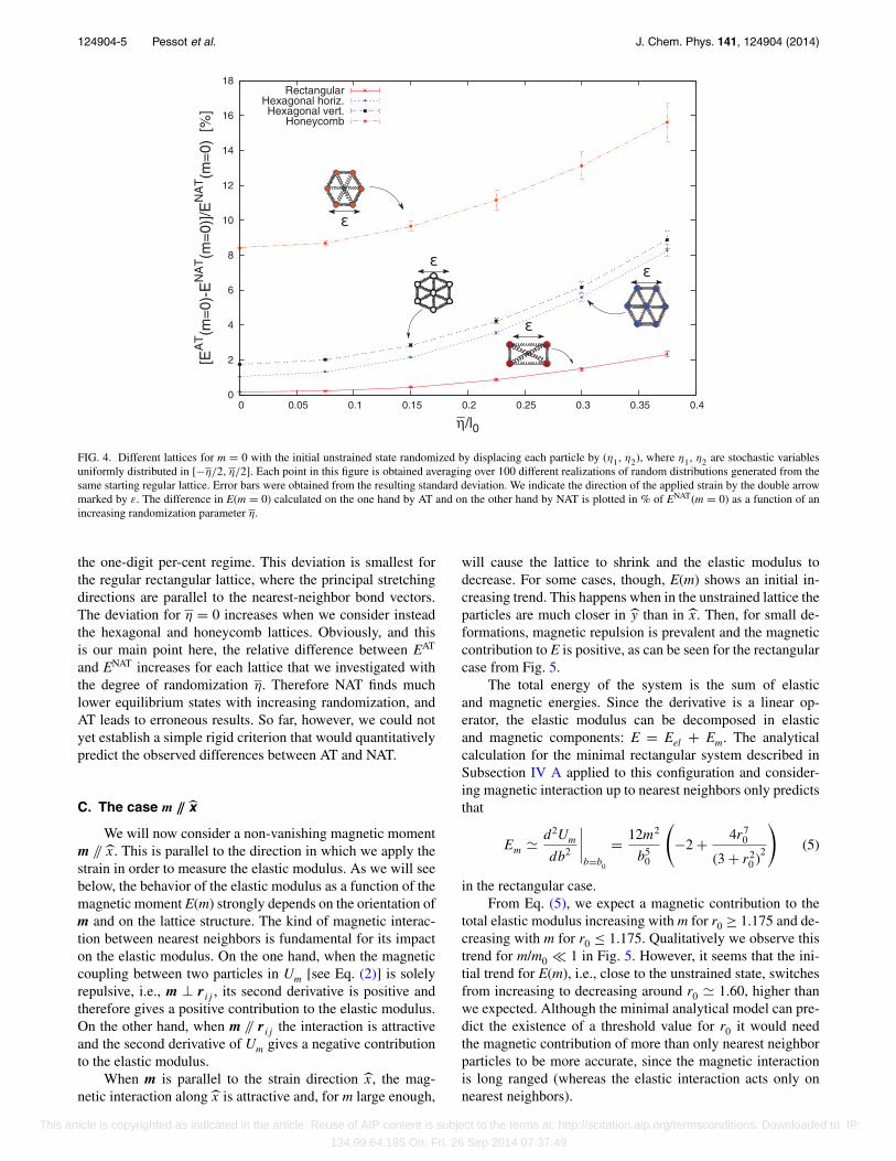
FIG. 4. Different lattices for m = 0 with the initial unstrained state randomized by displacing each particle by (η1, η2), where η1, η2 are stochastic variablesuniformly distributed in [−η/2, η/2]. Each point in this figure is obtained averaging over 100 different realizations of random distributions generated from thesame starting regular lattice. Error bars were obtained from the resulting standard deviation. We indicate the direction of the applied strain by the double arrowmarked by ε. The difference in E(m = 0) calculated on the one hand by AT and on the other hand by NAT is plotted in % of ENAT(m = 0) as a function of anincreasing randomization parameter η.

the one-digit per-cent regime. This deviation is smallest forthe regular rectangular lattice, where the principal stretchingdirections are parallel to the nearest-neighbor bond vectors.The deviation for η = 0 increases when we consider insteadthe hexagonal and honeycomb lattices. Obviously, and thisis our main point here, the relative difference between EAT

and ENAT increases for each lattice that we investigated withthe degree of randomization η. Therefore NAT finds muchlower equilibrium states with increasing randomization, andAT leads to erroneous results. So far, however, we could notyet establish a simple rigid criterion that would quantitativelypredict the observed differences between AT and NAT.

C. The case m // x

We will now consider a non-vanishing magnetic momentm // x. This is parallel to the direction in which we apply thestrain in order to measure the elastic modulus. As we will seebelow, the behavior of the elastic modulus as a function of themagnetic moment E(m) strongly depends on the orientation ofm and on the lattice structure. The kind of magnetic interac-tion between nearest neighbors is fundamental for its impacton the elastic modulus. On the one hand, when the magneticcoupling between two particles in Um [see Eq. (2)] is solelyrepulsive, i.e., m ⊥ r ij , its second derivative is positive andtherefore gives a positive contribution to the elastic modulus.On the other hand, when m // r ij the interaction is attractiveand the second derivative of Um gives a negative contributionto the elastic modulus.

When m is parallel to the strain direction x, the mag-netic interaction along x is attractive and, for m large enough,

will cause the lattice to shrink and the elastic modulus todecrease. For some cases, though, E(m) shows an initial in-creasing trend. This happens when in the unstrained lattice theparticles are much closer in y than in x. Then, for small de-formations, magnetic repulsion is prevalent and the magneticcontribution to E is positive, as can be seen for the rectangularcase from Fig. 5.

The total energy of the system is the sum of elasticand magnetic energies. Since the derivative is a linear op-erator, the elastic modulus can be decomposed in elasticand magnetic components: E = Eel + Em. The analyticalcalculation for the minimal rectangular system described inSubsection IV A applied to this configuration and consider-ing magnetic interaction up to nearest neighbors only predictsthat

Em � d2Um

db2

∣∣∣∣b=b0

= 12m2

b50

(−2 + 4r7

0

(3 + r20 )

2

)(5)

in the rectangular case.From Eq. (5), we expect a magnetic contribution to the

total elastic modulus increasing with m for r0 ≥ 1.175 and de-creasing with m for r0 ≤ 1.175. Qualitatively we observe thistrend for m/m0 � 1 in Fig. 5. However, it seems that the ini-tial trend for E(m), i.e., close to the unstrained state, switchesfrom increasing to decreasing around r0 � 1.60, higher thanwe expected. Although the minimal analytical model can pre-dict the existence of a threshold value for r0 it would needthe magnetic contribution of more than only nearest neighborparticles to be more accurate, since the magnetic interactionis long ranged (whereas the elastic interaction acts only onnearest neighbors).

This article is copyrighted as indicated in the article. Reuse of AIP content is subject to the terms at: http://scitation.aip.org/termsconditions. Downloaded to IP:

134.99.64.185 On: Fri, 26 Sep 2014 07:37:49

124904-6 Pessot et al. J. Chem. Phys. 141, 124904 (2014)

0.94

0.95

0.96

0.97

0.98

0.99

1

1.01

0 0.02 0.04 0.06 0.08 0.1

EN

AT(m

/m0)

/EN

AT(m

=0)

m/m0

r0=2.50r0=1.90r0=1.60r0=1.30r0=1.00

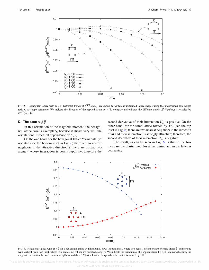
FIG. 5. Rectangular lattice with m // x. Different trends of ENAT(m/m0) are shown for different unstrained lattice shapes using the undeformed base-heightratio r0 as shape parameter. We indicate the direction of the applied strain by ε. To compare and enhance the different trends, ENAT(m/m0) is rescaled byENAT(m = 0).

D. The case m // y

In this orientation of the magnetic moment, the hexago-nal lattice case is exemplary, because it shows very well theorientational structural dependence of E(m).

On the one hand, for the hexagonal lattice “horizontally”oriented (see the bottom inset in Fig. 6) there are no nearestneighbors in the attractive direction y; there are instead twoalong x whose interaction is purely repulsive, therefore the

second derivative of their interaction Um is positive. On theother hand, for the same lattice rotated by π /2 (see the topinset in Fig. 6) there are two nearest neighbors in the directionof m and their interaction is strongly attractive; therefore, thesecond derivative of their interaction Um is negative.

The result, as can be seen in Fig. 6, is that in the for-mer case the elastic modulus is increasing and in the latter isdecreasing.

0.95

1

1.05

1.1

1.15

1.2

1.25

1.3

1.35

1.4

0 0.02 0.04 0.06 0.08 0.1 0.12 0.14 0.16

EN

AT(m

/m0)

/k

m/m0

ENAT vertical ENAT horizontal

FIG. 6. Hexagonal lattice with m // y for a hexagonal lattice with horizontal rows (bottom inset, where two nearest neighbors are oriented along x) and for onewith vertical rows (top inset, where two nearest neighbors are oriented along y). We indicate the direction of the applied strain by ε. It is remarkable how themagnetic interaction between nearest neighbors and the ENAT(m) behavior change when the lattice is rotated by π /2.

This article is copyrighted as indicated in the article. Reuse of AIP content is subject to the terms at: http://scitation.aip.org/termsconditions. Downloaded to IP:

134.99.64.185 On: Fri, 26 Sep 2014 07:37:49

124904-7 Pessot et al. J. Chem. Phys. 141, 124904 (2014)

FIG. 7. Elastic modulus E(m/m0)/k calculated with NAT for m // z for the different lattices shown. We indicate the direction of the applied strain by ε. Themagnetic interaction is purely repulsive and strengthens the elastic modulus in this configuration.

E. The case m // z

In this configuration, the magnetic interactions betweenour particles are all repulsive and have the form m2/rij

3. Thesecond derivative of the magnetic interparticle energy is al-ways positive along the direction connecting the particles.Therefore, we expect the elastic modulus to be enhanced withincreasing m, and E(m) to be a monotonically increasing func-tion. As can be seen from Fig. 7, this is true for all the differentlattices we have considered.

We have already seen in Fig. 4 how the randomizationof the lattice seriously affects the difference between AT andNAT. For the m // z case, we have also considered a real par-ticle distribution taken from an experimental sample.50 Thereal sample was of cylindrical shape with a diameter of about3 cm. It had the magnetic particles arranged in chain-like ag-gregates parallel to the cylinder axis and spanning the wholesample. The positions of the particles were obtained throughX-ray micro-tomography and subsequent image analysis. Weextracted the data from a circular cross-section taken approx-imately at half height of the cylinder and shown in Fig 8. Inthis way we consider by our model the physics of one cross-sectional plane of the cylindrical sample.

The extracted lattice was used as an input for our dipole-spring model. We placed a magnetic particle at the centerof each identified spot in the tomographic image, see Fig 8.Guided by the situation in the real sample, the magnetic mo-ments of the particles are chosen perpendicular to the plane(i.e., “along the cylinder axis”). The springs in the resultinglattice are set using Delaunay triangulation51, 57, 58 with theparticles at the vertices of the triangles and the springs placedat their edges. Then, we cut a square block from the centerof the sample containing the desired number of particles. Theclamped particles are chosen in such a way that they coverabout 10% of the total area (see left inset in Fig. 9).

FIG. 8. Realistic lattice used to determine the elastic modulus as a functionof the magnetic interactions in the case m // z. The lattice was determinedfrom an X-ray micro-tomographic image of a real experimental sample50 inthe following way. The sample was of cylindrical shape with a diameter ofapproximately 3 cm. We show a cross-sectional cut through the sample atintermediate height. Inside the sample, the magnetic particles formed chainsparallel to the cylinder axis, i.e., perpendicular to the depicted plane. Theaverage size of the particles was around 35 μm. Gray areas correspond tothe tomographic spots generated by the magnetic particles in the sample andwere identified by image analysis. In our model, we then used the centers ofthese spots, marked by the black boxes, as lattice sites. One magnetic parti-cle was placed on each lattice site. Then the whole plane was tessellated byDelaunay triangulation with the particle positions at the vertices of the result-ing triangles. Elastic springs were set along the edges of the triangles. Themicro-tomography data (see Fig. 5 (H=3 mm) in Ref. 50) are reproducedwith permission from Gunther et al., Smart Mater. Struct. 21, 015005 (2012).Copyright 2012 by IOP Publishing.

This article is copyrighted as indicated in the article. Reuse of AIP content is subject to the terms at: http://scitation.aip.org/termsconditions. Downloaded to IP:

134.99.64.185 On: Fri, 26 Sep 2014 07:37:49

124904-8 Pessot et al. J. Chem. Phys. 141, 124904 (2014)

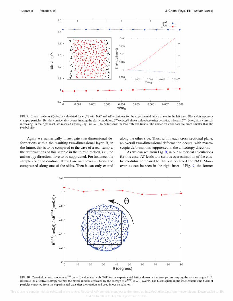
FIG. 9. Elastic modulus E(m/m0)/k calculated for m // z with NAT and AT techniques for the experimental lattice drawn in the left inset. Black dots representclamped particles. Besides considerably overestimating the elastic modulus, EAT(m/m0)/k shows a flat/decreasing behavior, whereas ENAT(m/m0)/k is correctlyincreasing. In the right inset, we rescaled E(m/m0) by E(m = 0) to better show the two different trends. The numerical error bars are much smaller than thesymbol size.

Again we numerically investigate two-dimensional de-formations within the resulting two-dimensional layer. If, inthe future, this is to be compared to the case of a real sample,the deformations of this sample in the third direction, i.e., theanisotropy direction, have to be suppressed. For instance, thesample could be confined at the base and cover surfaces andcompressed along one of the sides. Then it can only extend

along the other side. Thus, within each cross-sectional plane,an overall two-dimensional deformation occurs, with macro-scopic deformations suppressed in the anisotropy direction.

As we can see from Fig. 9, in our numerical calculationsfor this case, AT leads to a serious overestimation of the elas-tic modulus compared to the one obtained for NAT. More-over, as can be seen in the right inset of Fig. 9, the former

0

0.2

0.4

0.6

0.8

1

1.2

0 10 20 30 40 50 60 70 80 90

EN

AT(m

=0,

θ) /

<E

NA

T(m

=0,

θ)>

θ (degrees)

FIG. 10. Zero-field elastic modulus ENAT(m = 0) calculated with NAT for the experimental lattice drawn in the inset picture varying the rotation angle θ . Toillustrate the effective isotropy we plot the elastic modulus rescaled by the average of ENAT(m = 0) over θ . The black square in the inset contains the block ofparticles extracted from the experimental data after the rotation and used in our calculation.

This article is copyrighted as indicated in the article. Reuse of AIP content is subject to the terms at: http://scitation.aip.org/termsconditions. Downloaded to IP:

134.99.64.185 On: Fri, 26 Sep 2014 07:37:49

124904-9 Pessot et al. J. Chem. Phys. 141, 124904 (2014)

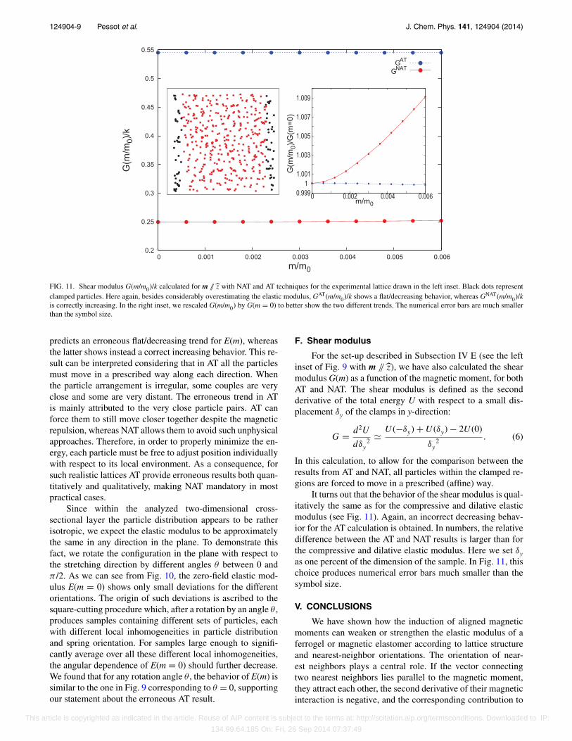
FIG. 11. Shear modulus G(m/m0)/k calculated for m // z with NAT and AT techniques for the experimental lattice drawn in the left inset. Black dots representclamped particles. Here again, besides considerably overestimating the elastic modulus, GAT(m/m0)/k shows a flat/decreasing behavior, whereas GNAT(m/m0)/kis correctly increasing. In the right inset, we rescaled G(m/m0) by G(m = 0) to better show the two different trends. The numerical error bars are much smallerthan the symbol size.

predicts an erroneous flat/decreasing trend for E(m), whereasthe latter shows instead a correct increasing behavior. This re-sult can be interpreted considering that in AT all the particlesmust move in a prescribed way along each direction. Whenthe particle arrangement is irregular, some couples are veryclose and some are very distant. The erroneous trend in ATis mainly attributed to the very close particle pairs. AT canforce them to still move closer together despite the magneticrepulsion, whereas NAT allows them to avoid such unphysicalapproaches. Therefore, in order to properly minimize the en-ergy, each particle must be free to adjust position individuallywith respect to its local environment. As a consequence, forsuch realistic lattices AT provide erroneous results both quan-titatively and qualitatively, making NAT mandatory in mostpractical cases.

Since within the analyzed two-dimensional cross-sectional layer the particle distribution appears to be ratherisotropic, we expect the elastic modulus to be approximatelythe same in any direction in the plane. To demonstrate thisfact, we rotate the configuration in the plane with respect tothe stretching direction by different angles θ between 0 andπ /2. As we can see from Fig. 10, the zero-field elastic mod-ulus E(m = 0) shows only small deviations for the differentorientations. The origin of such deviations is ascribed to thesquare-cutting procedure which, after a rotation by an angle θ ,produces samples containing different sets of particles, eachwith different local inhomogeneities in particle distributionand spring orientation. For samples large enough to signifi-cantly average over all these different local inhomogeneities,the angular dependence of E(m = 0) should further decrease.We found that for any rotation angle θ , the behavior of E(m) issimilar to the one in Fig. 9 corresponding to θ = 0, supportingour statement about the erroneous AT result.

F. Shear modulus

For the set-up described in Subsection IV E (see the leftinset of Fig. 9 with m // z), we have also calculated the shearmodulus G(m) as a function of the magnetic moment, for bothAT and NAT. The shear modulus is defined as the secondderivative of the total energy U with respect to a small dis-placement δy of the clamps in y-direction:

G = d2U

dδy2 � U (−δy) + U (δy) − 2U (0)

δy2 . (6)

In this calculation, to allow for the comparison between theresults from AT and NAT, all particles within the clamped re-gions are forced to move in a prescribed (affine) way.

It turns out that the behavior of the shear modulus is qual-itatively the same as for the compressive and dilative elasticmodulus (see Fig. 11). Again, an incorrect decreasing behav-ior for the AT calculation is obtained. In numbers, the relativedifference between the AT and NAT results is larger than forthe compressive and dilative elastic modulus. Here we set δyas one percent of the dimension of the sample. In Fig. 11, thischoice produces numerical error bars much smaller than thesymbol size.

V. CONCLUSIONS

We have shown how the induction of aligned magneticmoments can weaken or strengthen the elastic modulus of aferrogel or magnetic elastomer according to lattice structureand nearest-neighbor orientations. The orientation of near-est neighbors plays a central role. If the vector connectingtwo nearest neighbors lies parallel to the magnetic moment,they attract each other, the second derivative of their magneticinteraction is negative, and the corresponding contribution to

This article is copyrighted as indicated in the article. Reuse of AIP content is subject to the terms at: http://scitation.aip.org/termsconditions. Downloaded to IP:

134.99.64.185 On: Fri, 26 Sep 2014 07:37:49

124904-10 Pessot et al. J. Chem. Phys. 141, 124904 (2014)

the total elastic modulus is negative, too. If, instead, the near-est neighbors lie on a direction perpendicular to the magneticmoment, the second derivative of their magnetic interactionis positive and it tends to increase the total elastic modulus.This effect can be seen modifying the nearest-neighbor struc-ture, for instance tuning the shape of a rectangular lattice orrotating a hexagonal lattice. We have also seen how the perfor-mance of affine transformations worsens for randomized andmore realistic particle distributions, making non-affine trans-formation calculations mandatory when working with dataextracted from experiments.

In the present case, we scaled out the typical particle sep-aration and the elastic constant from the equations to keep thedescription general. Both quantities are available when realsamples are considered. The mean particle distance followsfrom the average density, while the elastic constant could beconnected to the elastic modulus of the polymer matrix.

The dipole-spring system we have considered is a mini-mal model. We look forward to improving it in different di-rections. First, we would like to go beyond linear elastic in-teractions using nonlinear springs, perhaps deriving a realisticinteraction potential from experiments or more microscopicsimulations. Second, the use of periodic boundary conditionsmay improve the efficiency of our calculations and give usnew insight into the system behavior (although we demon-strated by our study of asymptotic behavior that border ef-fects are negligible in the present set-up). Furthermore, wemay include a constant volume constraint, since volume con-servation is not rigidly enforced in the present model. To iso-late the effects of different lattice structures and the assump-tion of affine deformations, we here assumed that all magneticmoments are rigidly anchored along one given direction. In asubsequent step, this constraint could be weakened by explic-itly implementing the interaction with an external magneticfield or an orientational memory. Finally, to build the bridgeto real system modeling, an extension of our calculations tothree dimensions is mandatory in most practical cases.

ACKNOWLEDGMENTS

The authors thank the Deutsche Forschungsgemeinschaftfor support of this work through the priority program SPP1681.

1E. Jarkova, H. Pleiner, H.-W. Müller, and H. R. Brand, Phys. Rev. E 68,041706 (2003).

2P. M. Ajayan, L. S. Schadler, C. Giannaris, and A. Rubio, Adv. Mater. 12,750 (2000).

3S. Stankovich, D. A. Dikin, G. H. B. Dommett, K. M. Kohlhaas, E. J. Zim-ney, E. A. Stach, R. D. Piner, S. T. Nguyen, and R. S. Ruoff, Nature (Lon-don) 442, 282 (2006).

4S. C. Glotzer and M. J. Solomon, Nat. Mater. 6, 557 (2007).5J. Yuan, Y. Xu, and A. H. E. Müller, Chem. Soc. Rev. 40, 640 (2011).6G. Filipcsei, I. Csetneki, A. Szilágyi, and M. Zrínyi, Adv. Polym. Sci. 206,137 (2007).

7S. H. L. Klapp, J. Phys.: Condens. Matter 17, R525 (2005).8R. E. Rosensweig, Ferrohydrodynamics (Cambridge University Press,Cambridge, 1985).

9S. Odenbach, Colloid Surf., A 217, 171 (2003).10S. Odenbach, Magnetoviscous Effects in Ferrofluids (Springer,

Berlin/Heidelberg, 2003).11B. Huke and M. Lücke, Rep. Prog. Phys. 67, 1731 (2004).12S. Odenbach, J. Phys.: Condens. Matter 16, R1135 (2004).13P. Ilg, M. Kröger, and S. Hess, J. Magn. Magn. Mater. 289, 325 (2005).

14J. P. Embs, S. May, C. Wagner, A. V. Kityk, A. Leschhorn, and M. Lücke,Phys. Rev. E 73, 036302 (2006).

15P. Ilg, E. Coquelle, and S. Hess, J. Phys.: Condens. Matter 18, S2757(2006).

16C. Gollwitzer, G. Matthies, R. Richter, I. Rehberg, and L. Tobiska, J. FluidMech. 571, 455 (2007).

17G. Strobl, The Physics of Polymers (Springer, Berlin/Heidelberg, 2007).18M. Zrínyi, L. Barsi, and A. Büki, J. Chem. Phys. 104, 8750 (1996).19H.-X. Deng, X.-L. Gong, and L.-H. Wang, Smart Mater. Struct. 15, N111

(2006).20G. V. Stepanov, S. S. Abramchuk, D. A. Grishin, L. V. Nikitin, E. Y. Kra-

marenko, and A. R. Khokhlov, Polymer 48, 488 (2007).21X. Guan, X. Dong, and J. Ou, J. Magn. Magn. Mater. 320, 158 (2008).22H. Böse and R. Röder, J. Phys.: Conf. Ser. 149, 012090 (2009).23X. Gong, G. Liao, and S. Xuan, Appl. Phys. Lett. 100, 211909 (2012).24B. A. Evans, B. L. Fiser, W. J. Prins, D. J. Rapp, A. R. Shields, D. R. Glass,

and R. Superfine, J. Magn. Magn. Mater. 324, 501 (2012).25D. Y. Borin, G. V. Stepanov, and S. Odenbach, J. Phys.: Conf. Ser. 412,

012040 (2013).26K. Zimmermann, V. A. Naletova, I. Zeidis, V. Böhm, and E. Kolev, J. Phys.:

Condens. Matter 18, S2973 (2006).27D. Szabó, G. Szeghy, and M. Zrínyi, Macromolecules 31, 6541 (1998).28R. V. Ramanujan and L. L. Lao, Smart Mater. Struct. 15, 952 (2006).29T. L. Sun, X. L. Gong, W. Q. Jiang, J. F. Li, Z. B. Xu, and W. Li, Polym.

Test. 27, 520 (2008).30M. Babincová, D. Leszczynska, P. Sourivong, P. Cicmanec, and P. Babinec,

J. Magn. Magn. Mater. 225, 109 (2001).31L. L. Lao and R. V. Ramanujan, J. Mater. Sci.: Mater. Med. 15, 1061 (2004).32D. Ivaneyko, V. P. Toshchevikov, M. Saphiannikova, and G. Heinrich,

Macromol. Theor. Simul. 20, 411 (2011).33D. S. Wood and P. J. Camp, Phys. Rev. E 83, 011402 (2011).34P. J. Camp, Magnetohydrodynamics 47, 123 (2011).35O. V. Stolbov, Y. L. Raikher, and M. Balasoiu, Soft Matter 7, 8484 (2011).36D. Ivaneyko, V. Toshchevikov, M. Saphiannikova, and G. Heinrich, Con-

dens. Matter Phys. 15, 33601 (2012).37R. Weeber, S. Kantorovich, and C. Holm, Soft Matter 8, 9923 (2012).38A. Y. Zubarev, Soft Matter 8, 3174 (2012).39A. Y. Zubarev, Soft Matter 9, 4985 (2013).40A. Zubarev, Physica A 392, 4824 (2013).41Y. Han, W. Hong, and L. E. Faidley, Int. J. Solids Struct. 50, 2281 (2013).42D. Ivaneyko, V. Toshchevikov, M. Saphiannikova, and G. Heinrich, Soft

Matter 10, 2213 (2014).43M. A. Annunziata, A. M. Menzel, and H. Löwen, J. Chem. Phys. 138,

204906 (2013).44C. Garcia, Y. Zhang, F. DiSalvo, and U. Wiesner, Angew. Chem., Int. Ed.

42, 1526 (2003).45J. Kao, K. Thorkelsson, P. Bai, B. J. Rancatore, and T. Xu, Chem. Soc. Rev.

42, 2654 (2013).46E. Allahyarov, A. M. Menzel, L. Zhu, and H. Löwen, “Magnetomechanical

response of bilayered magnetic elastomers,” Smart Mater. Struct. (to bepublished); preprint arXiv:1406.6412 (2014).

47D. Collin, G. K. Auernhammer, O. Gavat, P. Martinoty, and H. R. Brand,Macromol. Rapid Commun. 24, 737 (2003).

48Z. Varga, J. Fehér, G. Filipcsei, and M. Zrínyi, Macromol. Symp. 200, 93(2003).

49S. Bohlius, H. R. Brand, and H. Pleiner, Phys. Rev. E 70, 061411 (2004).50D. Günther, D. Y. Borin, S. Günther, and S. Odenbach, Smart Mater. Struct.

21, 015005 (2012).51T. Borbáth, S. Günther, D. Y. Borin, T. Gundermann, and S. Odenbach,

Smart Mater. Struct. 21, 105018 (2012).52T. Gundermann, S. Günther, D. Borin, and S. Odenbach, J. Phys.: Conf.

Ser. 412, 012027 (2013).53J. J. Cerdà, P. A. Sánchez, C. Holm, and T. Sintes, Soft Matter 9, 7185

(2013).54P. A. Sánchez, J. J. Cerdà, T. Sintes, and C. Holm, J. Chem. Phys. 139,

044904 (2013).55M. R. Hestenses and E. Stiefel, J. Res. Natl. Bur. Stand. 49, 409 (1952).56J. R. Shewchuk, “An introduction to the conjugate gradient method with-

out the agonizing pain,” 1994, see http://www.cs.cmu.edu/~quake-papers/painless-conjugate-gradient.pdf.

57B. Delaunay, Bull. Acad. Sci. URSS. Cl. Sci. Math. Nat. 6, 793 (1934).58S. Pion and M. Teillaud, in CGAL User and Reference Manual, 4th

ed. (CGAL Editorial Board, 2014), see http://doc.cgal.org/4.4/Manual/packages.html#PkgTriangulation3Summary.

This article is copyrighted as indicated in the article. Reuse of AIP content is subject to the terms at: http://scitation.aip.org/termsconditions. Downloaded to IP:

134.99.64.185 On: Fri, 26 Sep 2014 07:37:49