Strategic Learning and the Topology of Social Networks

Elchanan Mossel∗, Allan Sly†and Omer Tamuz‡

June 2, 2015

Abstract

We consider a group of strategic agents who must each repeatedly take one of twopossible actions. They learn which of the two actions is preferable from initial privatesignals, and by observing the actions of their neighbors in a social network.

We show that the question of whether or not the agents learn efficiently dependson the topology of the social network. In particular, we identify a geometric “egalitar-ianism” condition on the social network that guarantees learning in infinite networks,or learning with high probability in large finite networks, in any equilibrium. We alsogive examples of non-egalitarian networks with equilibria in which learning fails.Keywords: Social learning, informational externalities, social networks, aggregationof information.

1 Introduction

Consider a group in which each agent faces a repeated choice between two actions. Initially,the information available to each agent is a private signal, which gives a noisy indication ofwhich is the correct action. As time progresses, the agents learn more by observing the actionsof their neighbors in a social network. They do not, however, obtain any direct indicationof the payoffs from their actions. For example, their choice could be one of lifestyle, whereone can learn by observing the actions of others, but where payoffs (e.g., longevity) are onlyrevealed after a large amount of time1.

We are interested in the question of learning, or aggregation of information: When isit the case that, through observing each other, the agents exchange enough information toconverge to the correct action? In particular, we are interested in the role that the geometryof the social network plays in this process, and in its effect on learning. Which social

∗University of Pennsylvania and University of California, Berkeley. E-mail: mossel@stat.berkeley.edu.Supported by NSF award DMS 1106999, by ONR award N000141110140 and by ISF grant 1300/08.†University of California, Berkeley. Supported by a Sloan Research Fellowship in mathematics and by

NSF award DMS 1208339‡Massachusetts Institute of Technology and Microsoft Research New England. This research was sup-

ported in part by a Google Europe Fellowship.1Consider parents who, each night, decide whether to lay their baby to sleep on its back or on its stomach.

They can learn by observing the actions of their peers, but presumably do not receive any direct feedbackregarding the effect of their actions on the baby’s health.

1

arX

iv:1

209.

5527

v2 [

cs.G

T]

30

May

201

5

networks enable the flow of information, and which impede it? This problem has been studiedextensively in the literature, using mostly boundedly-rational or heuristic approaches [10, 12,5, 11, 16, 17]. However, the basic question of how strategic agents behave in this setting hasbeen largely ignored2, perhaps because the model is mathematically difficult to approach,or because strategic behavior seems unfeasible3. This article aims to fill this gap. We definea notion of egalitarianism for social networks, and show that when agents are strategic,learning always occurs on egalitarian social networks, and may not occur on those that arenot egalitarian. Interestingly, these results broadly resemble those of some of the heuristicmodels (see, e.g., Golub and Jackson [16, Theorem 1]).

We call a social network graph (d, L)-egalitarian if it satisfies the following two conditions:(1) At most d edges leave each node (that is, each agent observes at most d others), and(2) whenever there is an edge from node i to j, there is a path back from j to i, of lengthat most L (that is, no agent is too far removed from those who observe her). In this articlewe show that on connected (d, L)-egalitarian graphs the agents learn the correct action, andgive examples of non-egalitarian graphs in which learning fails.

Our model is a discounted, repeated game with incomplete information. We consider astate of nature S which is equal to either 0 or 1, with equal probability. Each agent receivesa private signal that is independent and identically distributed conditioned on S, and iscorrelated with S. In each discrete time period t, each agent i chooses an action Ait takingvalues in 0, 1. The information available to her is her own private signal, as well as theactions of her social network neighbors in the previous time periods. Agent i’s stage utilityat time period t is equal to 1 if Ait = S and to 0 otherwise, and is discounted exponentially,by a common rate. We consider general Nash equilibria, and show that they indeed exist(Theorem D.5); this does not follow from standard results.

We say that agent i learns S when Ait is equal to S from some time on, and that learningtakes place when all agents learn S. Our main result (Theorem 1) is that on connected (d, L)-egalitarian graphs, in any equilibrium, learning occurs with high probability on large graphs,and with probability one on infinite graphs. We do not impose unbounded likelihood ratios:learning occurs in egalitarian networks even for weak - but informative - signals (contrastthis with the sequential learning case of Smith and Sørensen [28]). Note that this applies toall Nash equilibria, and therefore in particular to any perfect Bayesian equilibria. We alsoprovide examples of equilibria on large non-egalitarian networks in which, with non-vanishingprobability, the agents do not learn.

Our results require a smoothness condition on private signals: each private belief (theprobability that S = 1, conditioned on the private signal) must have a non-atomic distribu-tion. This ensures that agents are never (i.e., with zero probability) indifferent. Our resultsdo not, in general, hold without this condition; indifference can impede the flow of infor-mation (see, e.g., [23, Example A.1]). While real life signals are arguably always discreteor even finite, we propose that even with this requirement it is still possible to model orapproximate a large range of signals.

The model we study makes heavy demands on the agents in terms of rationality, com-mon knowledge, and human computation: agents are assumed to maximize a complicated

2Notable exceptions are [23] and [3]; we discuss these below.3See, e.g., Bala and Goyal [5]: “to keep the model mathematically tractable... this possibility [strategic

agents] is precluded in our model... simplifying the belief revision process considerably.”

2

expected utility function, to know the structure of the entire social network, and to preciselymake complicated inferences regarding the state of nature. While our approach is standardin this literature (see, e.g., [13, 26, 1]), these features of our model prompt us to present ourresults as benchmarks, rather than as predictive statements about the world.

The rest of this article proceeds as follows. In section 2 we discuss an example of a(d, L)-egalitarian graph, using it to provide intuition into the ideas behind our main result(Theorem 1). In Section 3 we provide two examples of non-egalitarian graphs on which theagents fail to learn. In Section 4 we introduce our model formally. In Section 5 we explorethe question of agreement and show that indeed the agents all converge to the same action.Section 6 includes our main technical contribution: a topology on equilibria of this game,as seen from the point of view of a particular agent. In Section 7 we prove Theorem 1, andSection 8 provides a conclusion.

1.1 Related literature

Learning on social networks is a widely studied field; a complete overview is beyond thescope of this paper, and so we shall note only a few related studies.

Bala and Goyal [5] study a similar model, and show results of learning or non-learningin different cases. Their model is boundedly-rational, with agents not taking into accountthe choices of their neighbors when forming their beliefs. Other notable bounded rationalitymodels of learning through repeated social interaction are those of DeGroot [10], Ellison andFudenberg [12], DeMarzo, Vayanos and Zwiebel [11], Golub and Jackson [16] and recentlyJadbabaie, Molavi and Tahbaz-Salehi [17]. Interestingly, a recurring theme is that learningis facilitated by graphs which are egalitarian, although notions of egalitarianism differ acrossmodels (see, e.g., Golub and Jackson [16, Property 2]).

In a previous paper [23], we consider the same question, but for myopic agents. Theanalysis in that case is far simpler and does not require the technical machinery that weconstruct in this article. More importantly, the conditions for learning are qualitativelydifferent for myopic agents, as compared to those for strategic agents: in the myopic setting,the upper bound on the number of observed neighbors is not needed. In fact, myopic agentslearn with high probability on networks with no uniform upper bound. Thus there areexamples of graphs on which myopic agents learn but strategic agents do not. We elaborateon this in our second example of non-learning, in Section 3.

In concurrent work by Arieli and Mueller-Frank [3], learning results are derived in astrategic setting with richer actions spaces; they study models in which actions are richenough to reveal beliefs, and show that in that case learning occurs under general conditions,and in particular for any graph topology. To the best of our knowledge, no previous workconsiders learning, in repeated interaction, on social networks, in a fully rational, strategicsetting.

The study of agreement (rather than learning) on social networks is also related to ourwork, and in fact we make crucial use of the work of Rosenberg, Solan and Vieille [26], whoprove an agreement result for a large class of games with informational externalities playedon social networks. This is a field of study founded by Aumann’s “Agreeing to disagree”paper [4], and elaborated on by Sebenius and Geanakoplos [27], McKelvey and Page [20],

3

Parikh and Krasucki [25], Gale and Kariv [13], Menager [21] and recently Mueller-Frank [24],to name a few. The moral of this research is that, by-and-large, rational agents eventuallyreach consensus, even in strategic settings. We elaborate on the work of Rosenberg, Solan andVieille [26] and show that when private signals are non-atomic then, asymptotically, agentsagree on best responses (Theorem 5.1). This agreement result is an important ingredient ofour main learning result (Theorem 1).

Another strain of related literature is that of herd behavior, started by Banerjee [6] andBikhchandani, Hirshleifer and Welch [8], with significant generalizations and further analysisby Smith and Sørensen [28], Acemoglu, Dahleh, Lobel and Ozdaglar [1] and recently Lobeland Sadler [19]. Here, the state of nature and private signals are as in our model, and agentsare rational. However, in these models agents act sequentially rather than repeatedly. Thesame informational framework is also shared by models of committee behavior and committeemechanism design (cf. Laslier and Weibull [18], Glazer and Rubinstein [14]).

1.2 Acknowledgments

We would like to thank Shahar Kariv for introducing us to this field. For commenting ondrafts of this paper we would like to thank Nageeb Ali, Ben Golub, Eva Lyubich, MarkusMobius, Ariel Rubinstein, Ran Shorrer, Glen Weyl, and especially Scott Kominers.

2 An illustrative example

T

T

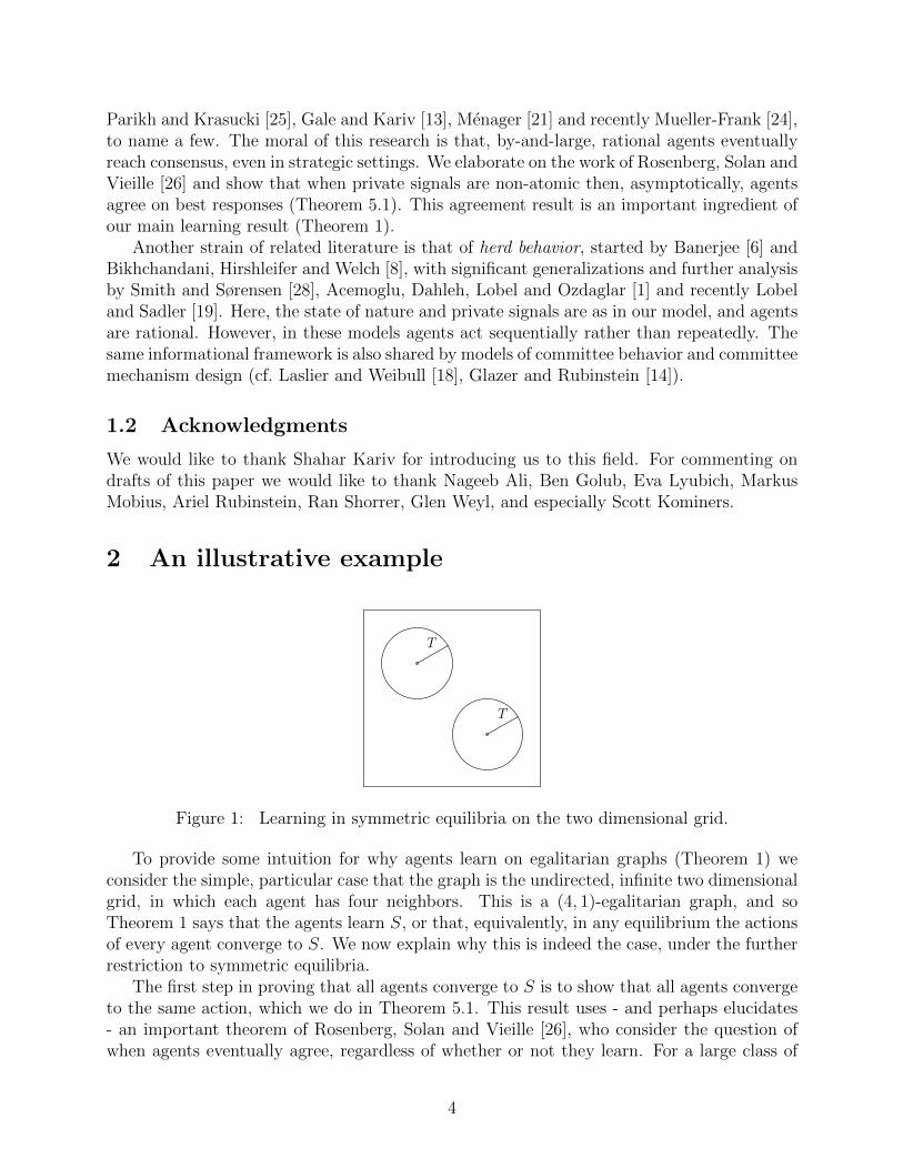
Figure 1: Learning in symmetric equilibria on the two dimensional grid.

To provide some intuition for why agents learn on egalitarian graphs (Theorem 1) weconsider the simple, particular case that the graph is the undirected, infinite two dimensionalgrid, in which each agent has four neighbors. This is a (4, 1)-egalitarian graph, and soTheorem 1 says that the agents learn S, or that, equivalently, in any equilibrium the actionsof every agent converge to S. We now explain why this is indeed the case, under the furtherrestriction to symmetric equilibria.

The first step in proving that all agents converge to S is to show that all agents convergeto the same action, which we do in Theorem 5.1. This result uses - and perhaps elucidates- an important theorem of Rosenberg, Solan and Vieille [26], who consider the question ofwhen agents eventually agree, regardless of whether or not they learn. For a large class of

4

games which includes the one we consider, they show that agents can disagree only if theyare indifferent. Our additional requirement of non-atomic private signals allows us to ruleout the possibility of indifference, and show that all agents converge to the same action4.

Having established that all agents converge to the same action, we use the fact that thegraph is symmetric, as is the equilibrium. Hence all agents converge at the same ex-anterate, and therefore, at some large enough time T , any particular agent will have converged,except with some very small probability ε. Of course, since the graph is infinite, there willbe at time T many agents who have yet to converge. However, if we consider any one agent(or two, as we do immediately below), the probability of non-convergence is negligible.

Now, consider two agents which are more than 2T edges apart on the graph (see Figure 1),and condition on the state of nature S equaling one. The two agents’ actions at time T areindependent random variables (conditioned on the state of nature), as they are too far apartfor any information to have been exchanged between them. On the other hand, since allagents converge to the same action, these independent random variables are equal (exceptwith probability ∼ 2ε); the two agents somehow, with high probability, reach the sameconclusion independently.

Now, two independent random variables that are equal must be constant. The agents’actions at time T are equal with high probability and independent conditioned on S, and soare with high probability equal to some fixed action. Since the agents’ signals are informative,this action is more likely to equal the state of nature than not (Claim G.4). Since this holdsfor every ε > 0, every agent’s limit action must equal the state of nature.

2.1 General egalitarian graphs

The formalization and extension of this intuition to general egalitarian graphs and general(i.e., non-symmetric) equilibria requires a significant technical effort, and in fact the con-struction of novel tools for the analysis of games on networks; to this we devote most of therest of this article. We now provide an overview of the main ideas.

The main notion we use is one of compactness. The two dimensional grid graph “looksthe same” from the point of view of every node: there is only one “point of view” in thisgraph. Such graphs as known as transitive graphs in the mathematics literature. Note thatthis is the only property of the grid that we used in the proof sketch above, and therefore thesame idea can be applied to all symmetric equilibria on infinite, connected transitive graphs.

We formalize a notion of an “approximate points of view”. We show that in particular,in an egalitarian graph, the nodes of the graph can be grouped into a finite number of sets,where from each set the graph “looks approximately the same”. Formally, we construct atopology in which the set of points of view in a graph is precompact if and only if the graphis (d, L)-egalitarian for some d and L (Theorem A.3). In this sense, egalitarianism, in whichthe set of points of view is precompact, is a relaxation of transitivity, in which the set ofpoints of view is a singleton. Indeed, transitivity is an extreme notion of egalitarianism, byany reasonable definition of an egalitarian graph.

This property of egalitarian graphs allows us to apply the intuition of the above example(or, more precisely, a similar intuition) to any infinite, (d, L)-egalitarian graph (Theorem I.1).

4In fact, Theorem 5.1 does not exclude the case that no agent converges at all; we will, for now, ignorethis possibility.

5

The fact that general equilibria are not symmetric is similarly treated by establishing thatthe space of equilibria is compact (Claim D.4). The theorem on finite graphs is proved byreduction to the case of infinite graphs.

Our main technical innovation is the construction of a topology on equilibria of thisgame, as seen from the point of view of a particular agent (Section 6.2). In this topology, anequilibrium has a finite number of “approximate points of view” if and only if the graph isegalitarian (Claim D.3). This topology is also useful for showing that equilibria exist in thecase of an infinite number of agents, which requires a non-standard argument (Theorem D.5).This technique should be applicable to the analysis of a large range of repeated, discountedgames on networks.

3 Non-learning

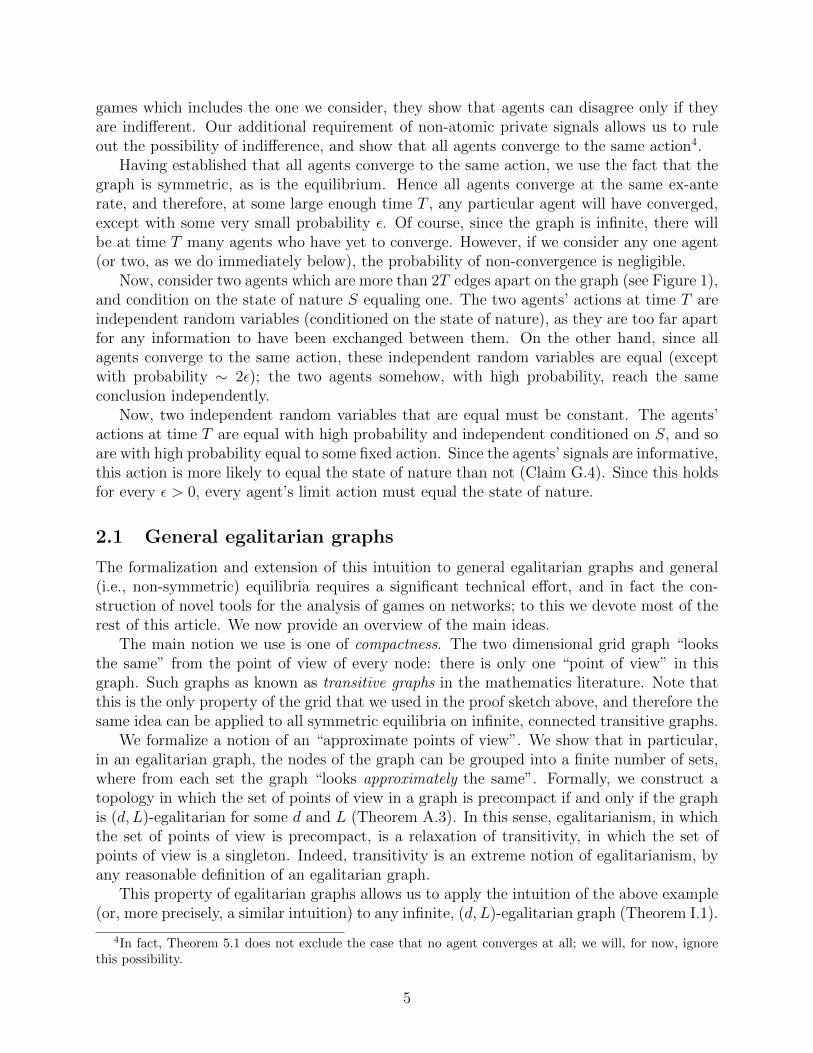
Figure 2: The Royal Family. Each member of the public (on the left), observes each royal(on the right), as well as her next door neighbors. The royals observe each other, and oneroyal observes one member of the public.

We provide two example of non-egalitarian graphs in which the agents do not learn.In the first example (Figure 2), inspired by Bala and Goyal’s royal family graph [5], thesocial network has two groups of agents: a “royal family” clique of R agents who all observeeach other, and n agents - the “public” - who are connected in an undirected chain, andadditionally can observe all the agents in the royal family. Finally, a single member of theroyal family observes one of the public, so that the graph is connected5. We think of R asfixed and consider the case of arbitrarily large n, or even infinite n.

While this graph satisfies condition (1) of egalitarianism, it violates condition (2). There-fore, Theorem 1 does not apply. Indeed, in the online appendix we construct an equilibriumfor the game on this network, in which the agents of the public ignore their own privatesignals after observing the first action of the royal family, which provides a much strongerindication of the correct action. However, the probability that the royal family is wrong isindependent of n: since the size of the royal family is fixed, with some fixed probability everyone of its members is mislead by her private signal to choose the wrong action in the firstperiod. Hence, regardless of how large society is, there is a fixed probability that learningdoes not occur.

5The graph is, in fact, strongly connected, meaning that there is a directed path connecting every orderedpair of agents.

6

king

regent

court

bureaucracy

people

Figure 3: The mad king. In this social network all edges are bi-directional. Each memberof the people is connected only to the king, as is each member of the court. The membersof the bureaucracy are connected only to the regent.

We construct a second example of non-learning which we call “the mad king”. Here, thegraph is undirected, so that whenever i observes j then j observes i; the graph thereforesatisfies condition (2) of egalitarianism with L = 1, but not condition (1). The graph(see Figure 3) consists of five types: the people, the king, the regent, the court and thebureaucracy. There is one king, one regent, a fixed number of members of the court anda fixed number of members of the bureaucracy, which is much larger than the court. Thenumber of people is arbitrarily large. They are connected as follows:

• The king is connected to the regent, the court and the people.

• The regent is connected to the king and to the bureaucracy.

• The members of the court are each connected only to the king.

• The members of the bureaucracy are each connected only to the regent.

• Importantly, the people are each connected only to the king, and not to each other.

For an appropriate choice of private signal distributions and discount factor, we constructan equilibrium in which all agents act myopically in the first two rounds, except for thepeople, who choose the constant action 0. This is enforced by a threat from the king, who, ifany of the people deviate, will always play 1, denying them any information he has learned;the prize for complying is the exposure to a well informed action which first aggregatesthe information available to the court, and later aggregates the information available to the(larger) bureaucracy. The result is that the information in the people’s private signals is lost,and so we have non-learning with probability bounded away from 0, for graphs of arbitrarilylarge size.

The equilibrium path can be succinctly described as follows; we provide a completedescription in the online appendix:

7

• The members of the bureaucracy act myopically in round 0, as do the members of thecourt.

• The regent, who learns by observing the bureaucracy, acts myopically at time 0 andat time 1. Therefore, and since the bureaucracy is large, his action at time 1 will becorrect with some fixed high probability.

• The king acts myopically in round 0. At round 1, after having learned from the court’sactions, the king again acts myopically, unless any of the people chose action 1 at round0, in which case he chooses action 1 at this time and henceforth.

• The people choose action 0 in round 0. They have no incentive to deviate, since theystand to learn much from the king’s actions, which, at the next round, will aggregatethe information in the court’s actions.

• By round 2, the king has learned from the regent’s well informed action of round 1. Hetherefore, at round 2, emulates the regent’s action of round 1, unless any of the peoplechose action 1 at rounds 0 or 1, in which case he again chooses action 1 at this timeand henceforth.

• In round 1 the people again choose action 0. They again have no reason to deviate, thistime because they wish to learn the regent’s action, through the king; this information- which originates from the bureaucracy - is much more precise than that which thethe king collected from the court in the previous round and reveals to them in thisround.

• At round 2 (and henceforth) the people emulate the king’s previous action, and there-fore the king will not learn from them.

It follows that the private signals of the people are lost, and so, regardless of the number ofpeople, there is a fixed probability of non-learning.

We were not able to prove - or to disprove - that this equilibrium is a perfect Bayesianequilibrium. However, it intuitively seems likely that if the people were to deviate fromthe equilibrium, then the king would not have an incentive to carry out his threat. If thisintuition holds then this is not a perfect Bayesian equilibrium.

An interesting phenomenon is that on this graph, the agents do learn S with high proba-bility when they discount the future sufficiently, or in the limiting case that they are myopic(i.e., fully discount the future). This is thus an example - and perhaps a counter-intuitiveone - of how strategic agents may learn less effectively than myopic ones.

4 Model

4.1 Informational structure

The structure of the private information available to the agents is the standard one used inthe herding literature (see, e.g., Smith and Sørensen [28]).

8

We denote by V the set of agents, which we take to equal 1, 2, . . . , n in the finite caseand N = 1, 2, . . . in the (countably) infinite case. Let 0, 1 be the set of possible valuesof the state of nature S, and let P [S = 1] = P [S = 0] = 1/2. Let Ω be a measurable space,called the space of private signals. Let Wi ∈ Ω be agent i’s private signal, and denoteW = (W1,W2, . . .). Fix µ0 and µ1, two mutually absolutely continuous probability measureson Ω. Conditioned on S = 0, let Wi be i.i.d. µ0, and conditioned on S = 1 let Wi be i.i.d.µ1.

The assumption that P [S = 1] = 1/2 can be relaxed; in particular, for every choice ofprivate signals there exist p1 < 1/2 < p2 such that our results apply when P [S = 1] istaken to be in (p1, p2). However, when agents are myopic (or more generally discount thefuture enough), when priors are skewed, and when signals are weak, then regardless of thegraph, and in any equilibrium, agents will disregard their private signals and only play themore a priori probable action. Indeed, if for example the prior is P [S = 1] = 0.8, then forweak enough private signals it will be the case that P [S = 1|Wi] > 0.7 with probability one.Myopic agents always choose the action that they deem more likely to equal the state of theworld, and therefore will choose 1, as will agents who are not myopic but sufficiently discountthe future. It follows that in this case observing others’ actions will reveal no information,and no learning will occur. Therefore, to ensure learning, one must impose some conditionson the prior and the strength of the private signals; for example, a sufficient condition wouldbe that P [S = 1|Wi] has positive probability of both being above half and of being belowhalf. To avoid encumbering this paper with an additional layer of technical complexity, wefocus on the case in which P [S = 1] = P [S = 0] = 1/2.

Agent i’s private belief Ii is the probability that the state of the world is 1, given i’sprivate signal:

Ii = P [S = 1|Wi] .

Since Ii is a sufficient statistic for S given Wi, we assume below without loss of generalitythat an agent’s actions depend on Wi only through Ii (see, e.g., Smith and Sørensen [28]).

We consider only µ0 and µ1 such that the distribution of Ii is non-atomic. This isthe condition that we refer to above as non-atomic private beliefs. This is an additionalrestriction that we impose, beyond what is standard in the herding literature.

4.2 The social network

The agents’ social network defines which of them observe the actions of which others. Wedo not assume that this is a symmetric relation: it may be that i observes j while j doesn’tobserve i. Formally, the social network G = (V,E) is a directed graph: V is the set of agents,and E is a relation on V , or a subset of the set of ordered pairs V ×V . The set of neighborsof i ∈ V is

N(i) = j : (i, j) ∈ E,

and we consider only graphs in which i ∈ N(i); that is, we require that an agent observesher own actions. The out-degree of i is given by |N(i)|, and will always be finite. This meansthat an agent observes the actions of a finite number of other agents. We do allow infinite

9

in-degrees; this corresponds to agents whose actions are observed by infinitely many otheragents.

Let G = (V,E) be a directed graph. A (directed) path of length k from i ∈ V to j ∈ V inG is sequence of k+ 1 nodes i1, . . . , ik+1 such that (in, in+1) ∈ E for n = 1, . . . , k, and wherei1 = i and ik+1 = j.

A directed graph is strongly connected if there exists a directed path between every orderedpair of nodes; we restrict our attention to such graphs. Strong connectedness is natural inthe contexts of agreement and learning; as an extreme example, consider a graph in whichsome agent observes no-one. In this graph we cannot hope for that agent to learn the stateof nature.

A directed graph G is L-locally-connected if, for each (i, j) ∈ E, there exists a path oflength at most L in G from j to i. Equivalently, G is L-locally-connected if whenever thereexists a path of length k from i to j, there exists a path of length at most L · k from j backto i. Note that 1-locally-connected graphs are commonly known as undirected graphs.

As defined above, a graph is said to be (d, L)-egalitarian if all out-degrees are boundedby d, and if it is L-locally-connected.

4.3 The game

To model the agents’ strategic behavior we consider the following game of incomplete infor-mation. This framework, with some variations, has been previously used, for example, byGale and Kariv [13] and Rosenberg, Solan and Vieille [26].

We consider the discrete time periods t = 0, 1, 2, . . ., where in each period each agenti ∈ V has to choose one of the actions in 0, 1. The information available to i at timet is her own private signal (of which the relevant information is her private belief, takingvalues in [0, 1]), and the actions of her neighbors in previous time periods, taking values in0, 1|N(i)|·t. This action is hence calculated by some function from [0, 1] × 0, 1|N(i)|·t to0, 1.

A pure strategy at time t of an agent i ∈ V is therefore a Borel-measurable functionqit : [0, 1] × 0, 1|N(i)|·t → 0, 1. A pure strategy of an agent i is the sequence of functionsqi = (qi0, q

i1, . . .), where qit is i’s pure strategy at time t. We endow the space of pure strategies

with the topology derived from the weak topology on functions from [0, 1] to 0, 1.A mixed strategy Qi of agent i is a pure-strategy-valued random variable; this is the

standard notion of a mixed strategy, and we shall henceforth refer to mixed strategies simplyas strategies. A (mixed) strategy profile is a set of strategies Q = Qi : i ∈ V , where therandom variables Qi are independent of each other and of the private signals.

The action of agent i at time t is denoted by Ait ∈ 0, 1. Denote the history of actions

of the neighbors of i before time t by AN(i)[0,t) = Ajs : s < t, j ∈ N(i); this depends on the

social network G. The action that agent i plays at time t under strategy profile Q is

Ait = Ait(G, Q) = Qit

(Ii, A

N(i)[0,t)

).

Note again that we (without loss of generality) limit the action to be a function of theprivate belief Ii, as opposed to the private signal Wi.

10

Let 0 < λ < 1 denote the agents’ common discount factor. Given a social network G andstrategy profile Q, agent i’s stage utility at time t, Ui,t, is 1 if her action matches S, and 0otherwise:

Ui,t = Ui,t(G, Q) = 1Ait(G,Q)=S.

Her expected stage utility at time t, ui,t, is therefore given by

ui,t = ui,t(G, Q) = E[Ui,t(G, Q)

]= P

[Ait(G, Q) = S

].

Agent i’s expected utility ui is given by

ui = ui(G, Q) = (1− λ)∞∑t=0

λtui,t(G, Q).

Note that ui ∈ [0, 1], due to the normalization factor (1 − λ). A game G is a 4-tuple(µ0, µ1, λ,G) consisting of two measures, a discount factor and a social network graph, sat-isfying the conditions of the definitions above.

4.4 Equilibria

Our equilibrium concept is the standard Nash equilibrium in games of incomplete informa-tion: Q is an equilibrium if no agent can improve her expected utility ui(Q) by deviatingfrom Q.

Formally, in a game G = (µ0, µ1, λ,G), strategy profile Q is an equilibrium if, for everyagent i ∈ V it holds that

ui(G, Q) ≥ ui(G, R),

for any R such that Rj = Qj for all j 6= i in V .

5 Agreement

Let the infinite action set Ci of agent i be defined by

Ci = Ci(G, Q) = s ∈ 0, 1 : Ait(G, Q) = s for infinitely many values of t.

There could be more than one action that i takes infinitely often. In that case we writeCi = 0, 1. Otherwise, with a slight abuse of notation, we write Ci = 0 or Ci = 1, asappropriate.

In this section we show that the agents reach consensus in any graph, in the followingsense:

Theorem 5.1. Let G be a game with either finitely many players or countably infinitelymany players, and let Q be an equilibrium strategy profile of G. Then, with probability one,Ci = Cj for all agents i, j ∈ V .

11

This theorem is a crucial ingredient in the proof of the main result of this article. Indeed,learning occurs if Ci = S for all i, and so a prerequisite is that Ci = Cj for all i, j.

Recall that a strategy of agent i at time t is a function of her private belief Ii and theactions of her neighbors in previous time periods, A

N(i)[0,t) . Hence we can think of the sigma-

algebra generated by these random variables as the “information available to agent i at timet”. Denote the information available to agent i at time t by

F it = F it (G, Q) = σ(Ii, Q

i, AN(i)[0,t)

),

and denote by

F i∞ = F i∞(G, Q) = σ(∪∞t=0F it

)the information available to agent i at the limit t → ∞. Note that F it includes the sigma-algebra generated by i’s private belief, the actions of i’s neighbors before time t, and i’s purestrategy; i knows which pure strategy she has chosen.

Since the expected stage utility of action s at time t is P [s = S], a myopic agent wouldtake an action s in 0, 1 that maximizes P [s = S|F it ]. This motivates the following defini-tion. Denote the best response of agent i at time t by

Bit = Bi

t(G, Q) = argmaxs∈0,1

P[s = S

∣∣F it (G, Q)].

Likewise denote the set of best responses of agent i at the limit t→∞ by

Bi∞ = Bi

∞(G, Q) = argmaxs∈0,1

P[s = S

∣∣F i∞] .At any time t there is indeed almost surely only one action that maximizes P

[s = S

∣∣F it (G, Q)],

since we require that the distribution of private beliefs be non atomic. This does not nec-essarily hold at the limit t → ∞, and so we let Bi

∞ take the values 0, 1 or 0, 1. Notethat a reasonable conjecture is that the probability that Bi

∞ = 0, 1 is zero, but we are notable to prove this. This does not, however, prevent us from proving our results, but it doescomplicate the proofs.

The following theorem is a restatement, in our notation, of Proposition 2.1 in Rosenberg,Solan and Vieille [26].

Theorem 5.2 (Rosenberg, Solan and Vieille). For any agent i it holds that Ci ⊆ Bi∞ almost

surely, in any equilibrium.

That is, any action that i takes infinitely often is optimal, given all the information agenti eventually learns. Note that this theorem is stated in [26] for a finite number of agents.However, a careful reading of the proof reveals that it holds equally for a countably infiniteset of agents. The same holds for their Theorem 2.3, in which they further prove the followingagreement result.

Theorem 5.3 (Rosenberg, Solan and Vieille). Let j be a neighbor of i. Then Cj ⊆ Bi∞

almost surely, in any equilibrium.

12

Equivalently, if i observes j, and j takes an action a infinitely often, then a is an optimalaction for i. If we could show that Bi

∞ = Ci for all i, it would follow from these two theorems,and from the fact that the graph is strongly connected, that Ci = Cj for all agents i andj; the agents would agree on their optimal action sets. This is precisely what we show inTheorem E.3. Our agreement theorem (Theorem 5.1) is a direct consequence.

6 Topologies on graphs and strategy profiles

6.1 Rooted graphs and their topology

A rooted graph is a pair (G, i), where G = (V,E) is a directed graph, and i ∈ V is a vertexin G.

Rooted graphs are a basic mathematical concept, and are important to the understandingof this game. This section starts with some basic definitions, continues with the definition of ametric topology on rooted graphs, and culminates in a novel theorem on compactness in thistopology, which may be of independent interest. In this we follow our previous work [23],which builds on the work of others such as Benjamini and Schramm [7] and Aldous andSteele [2].

Intuitively, a rooted graph is a graph, as seen from the “point of view” of a particularvertex - the root. Two rooted graphs will be close in our topology if the two graphs aresimilar, as seen from the roots.

Before defining our topology we will need a number of standard definitions. Let G =(V,E) and G′ = (V ′, E ′) be graphs, and let (G, i) and (G′, i′) be rooted graphs. A rootedgraph isomorphism between (G, i) and (G′, i′) is a bijection h : V → V ′ such that

1. h(i) = i′.

2. (j, k) ∈ E ⇔ (h(j), h(k)) ∈ E ′.

If there exists a rooted graph isomorphism between (G, i) and (G′, i) then we say that theyare isomorphic, and write (G, i) ∼= (G′, i′). Informally, isomorphic graphs cannot be toldapart when vertex labels are removed; equivalently, one can be turned into the other by anappropriate renaming of the vertices. The isomorphism class of (G, i) is the set of rootedgraphs that are isomorphic to it, and will be denoted by [G, i].

Let j, k be vertices in a graph G. Denote by ∆(j, k) the length of the shortest (directed)path from j to k. In general, ∆(j, k) 6= ∆(k, j), since the graph is directed. The (directed)ball Br(G, i) of radius r of the rooted graph (G, i) is the rooted graph, with root i, inducedin G by the set of vertices j ∈ V : ∆(i, j) ≤ r.

We now proceed to define our topology on the space of isomorphism classes of stronglyconnected rooted graphs, which is an extension of the Benjamini-Schramm [7] topology onundirected graphs. We define this topology by a metric6.

6 This definition applies, in fact, to a larger class of directed graphs: a rooted graph (G, i) is weaklyconnected if there is a directed path from i to each other vertex in the graph. Note that indeed a stronglyconnected graph is necessarily weakly connected, but not vice versa. Note also that a rooted graph (G, i) isweakly connected if and only if for every vertex j there exists an r such that j is in Br(G, i).

13

Let [G′, i′] and [G, i] be isomorphism classes of strongly connected rooted graphs. Thedistance D([G, i], [G′, i′]) is defined by

D([G, i], [G′, i′]) = inf2−r : Br(G, i) ∼= Br(G′, i′). (1)

That is, the larger the radius around the roots in which the graphs are isomorphic, the closerthey are. In fact, the quantitative dependence of D(·, ·) on r (exponential in our definition)will not be of importance here, as we shall only be interested in the topology induced by thismetric.

It is straightforward to show that D(·, ·) is well defined; a standard diagonalization ar-gument (which we use repeatedly in this article) is needed to show that it is indeed a metricrather than a pseudometric (Claim A.1). The assumption of strong connectivity is crucialhere, since D(·, ·) is otherwise a pseudometric.

Let SCG be the set of isomorphism classes of strongly connected rooted graphs. This setis a topological space when equipped with the topology induced by the metric D(·, ·). Givena strongly connected graph G, let R(G) ⊂ SCG be the set of all rooted graph isomorphismclasses of the form [G, i], for i a vertex in G. This can be thought of as the set of “points ofview” in the graph G. The notion of (d, L)-egalitarianism now arises naturally, in the sensethat the number of “approximate points of view” in G is finite if and only if G is egalitarian.This is formalized in the following lemma.

Lemma 6.1. Let G be a strongly connected graph. Then the closure of R(G) is compact inSCG if and only if G is (d, L)-egalitarian, for some d and L.

We would like to suggest that Lemma 6.1, which we prove in Appendix A, may be ofindependent mathematical interest, as it extends the well understood notion of compactnessin undirected graphs to directed, strongly connected graphs.

6.2 The space of rooted graph strategy profiles and its topology

In this section we use the above topology on rooted graphs to construct a topology on whatwe call rooted graph strategy profiles. This will be the main tool at our disposal in provingboth the existence of equilibria, and our main result, Theorem 1. Intuitively, a rooted graphstrategy profile will be a graph, together with a strategy profile, as seen from the point ofview of the root. As in the case of rooted graphs, two points in this space will be close ifthey look alike from the points of view of the roots.

Let G = (V,E) and G′ = (V ′, E ′) be strongly connected directed graphs, and let(G, i), (G′, i′) ∈ SCG be rooted graphs. Let Q and R be strategy profiles for the agents in Vand V ′, respectively. We say that the triplet (G, i, Q) is equivalent to the triplet (G′, i′, R)if there exists a rooted graph isomorphism h from (G, i) to (G′, i′) such that Qj = Rh(j) forall j ∈ V . The rooted graph strategy profiles GS are the set of equivalence classes inducedby this equivalence relation. We denote an element of GS by [G, i, Q].

In Appendix C we apply the classical work of Milgrom and Weber [22] to define a metricd on a single agent’s strategy space, with the property that when the number of agents isfinite then utilities are continuous in the induced topology.

We use this metric, and the metric of rooted graphs to define a metric on rooted graphstrategy profiles. Intuitively, [G, i, Q] and [G′, i′, R] will be close in this metric if, in a large

14

radius around i and i′, it holds both that the graphs are isomorphic and that the strategiesare similar.

Let d be a metric on a single agent’s strategy space. Let i and i′ be agents in graphsG and G′, respectively. We can use d as a metric between their strategies, as long as weuniquely identify each neighbor of one with a neighbor of the other. Let h be a bijectionbetween N(i′) and N(i). Then dh(Q

i, Qi′) will denote the distance thus defined between Qi

and Qi′ .We next define Dr(·, ·), a pseudometric on graph strategy profiles which only takes into

account the graph and the strategies at balls of radius r around the root. Two graph strategyprofiles are close in Dr if (1) these balls are isomorphic, so that agents in these balls can beidentified, and if (2) under some such identification, identified agents have similar strategies.This is a pseudometric rather than a metric since there could be two graph strategy profilesthat are at distance 0 under Dr, but are not identical; differences will, however, occur onlyat distances that are larger than r from the roots.

Let [G, i, Q] and [G′, i′, R] be rooted graph strategies. For r ∈ N, let H(r) be the (perhapsempty) set of rooted graph isomorphisms between Br(G, i) and Br(G

′, i′). Let

Dr

([G, i, Q], [G′, i′, R]

)= min

h∈H(r+1)max

j∈Br(G,i)dh(Q

j, Rh(j)),

when H(r + 1) is non-empty, and 1 otherwise. The choice of h ∈ H(r + 1) and thenj ∈ Br(G, i) guarantees that h is a bijection from the set of neighbors of j to the set ofneighbors of h(j).

Finally, define the metric D([G, i, Q], [G′, i′, R]) by

D(

[G, i, Q], [G′, i′, R])

= infr∈N

max

2−r, Dr([G, i, Q], [G′, i′, R])

. (2)

Note that D will be small whenever Dr is small for large r. It is straightforward (if tedious)to show that D(·, ·) is indeed a well defined metric.

6.3 Properties of the space of rooted graph strategy profiles

Two rooted graph strategy profiles will be close in the topology induced by D if, in a largeneighborhood of the roots, it holds both that the graphs are isomorphic, and also that thestrategies are similar. This captures the root’s “point of view” of the entire strategy profile.

While many possible topologies may have this property, this topology has some technicalfeatures that make it a useful analytical tool. First, expected utilities are continuous is thistopology. Formally, let the utility map u : GS → R be given by

u([G, i, Q]) = ui(G, Q).

This is a straightforward recasting of the previous definition of expected utility into thelanguage of rooted graph strategy spaces. In Lemma D.1 we show that u : GS → R iscontinuous; this follows from the fact that payoff is discounted, and so the strategies offar away agents have only a small effect on an agent’s utility. Another property of thistopology that makes it applicable is that the set of equilibrium rooted graph strategy profiles

15

is closed (Lemma D.2). These properties are also instrumental in proving that equilibriaexist (Theorem D.5).

Additionally, the probability of learning is lower semi-continuous in this topology. Letthe probability of learning map p : GS → R be given by

p([G, i, Q]) = limt→∞

P[Ait(G, Q) = S

].

In Section G we prove that p is well defined and that it is lower semi-continuous (Theo-rem G.5). We also show that p([G, i, Q]) = 1 if and only if the agents learn; i.e., if and onlyif limtA

jt = S almost surely for all agents j in G (Claim G.3).

Finally, if G is an egalitarian graph, then the set of rooted graph strategy profiles on Gis precompact (Claim D.3). Intuitively, this means that when G is egalitarian then not onlyare there finitely many approximate points of view of the graph (as discussed above), butalso just finitely many approximate points of view of the strategy profile.

7 Learning

7.1 Learning on infinite egalitarian graphs

Let G be an infinite, connected, (d, L)-egalitarian graph, and let Q be an equilibrium strategyprofile. In this section we show that all agents learns S almost surely.

Recall that all agents converge to the same (random) action or set of actions. Denoteby S∞ the random variable that is equal to 0 if all agents converge to 0 and is equal to1 if all agents converge to 1, or if they all do not converge. Our choice of notation herefollows from the fact that S∞ is a maximum a posteriori (MAP) estimator of any particularagent, given all that it learns: namely, the probability that an agent learns S is equal to theprobability that S∞ equals S (Claim G.1). Since the private signals are informative, S∞ = Swith probability which is strictly greater than one half (Claim G.4), so S∞ is a non-trivialestimator of S.

Note that S∞ is measurable in the sequence of every agent’s actions. Hence each agenteventually learns it, or something “close to it” at large finite times: formally, for every δ > 0there will be a time t and random variable Si,δ∞ that can be calculated by i at time t, and

such that P[Si,δ∞ = S∞

]> 1− δ.

Now, S∞ is a deterministic function of the agents’ private signals and pure strategies.Hence (e.g., by the martingale convergence theorem) S∞ is an almost deterministic functionof the private signals and pure strategies of a large but finite group of agents. Formally, forevery ε > 0 there is a random variable Sε∞ that depends only on the private signals and pure

strategies of some finite set of agents V ε, and such that P[Sε∞ = S∞

]> 1− ε.

Let i be an agent who is far away (in graph distance) from V ε, so that the nearestmember of V ε is at distance at least t from i. Then everything that i observes up to timet is independent of Sε∞, and hence “approximately independent” of S∞ (Claim H.4); weformalize a notion of “approximate independence” in Section F.

Now, as we note above, i eventually learns S∞ (or more precisely an estimator Si,δ∞ thatis equal to S∞ with high probability), gaining a new estimator of S which is (approximately)

16

independent of any estimators that it has learned up to time t. What we have so far outlinedcan thus be summarized informally as follows: the estimator S∞ is “decided upon” by a finitegroup of agents. When those far away eventually learn it they gain a new, approximatelyindependent estimator of S.

We apply this argument inductively, relying crucially on the fact that the space of rootedgraph strategies on G is precompact: Assume by induction that for every “point of view”[H, j, R] in the closure of this space there is an agent i in H with k − 1 approximatelyindependent estimators of S by some time t. By compactness and the infinitude of G, thereare infinitely many agents in G whose points of view are approximately equal to that of suchan agent i. These will all also have k−1 approximately independent estimators of S by timet. Some (in fact, almost all) of these agents will be sufficiently far from V ε. These will thengain a new estimator when they eventually learn S∞.

Hence in egalitarian graph, for any k and any degree of approximation, there will alwaysbe an agent who, given enough time, will accumulate k approximately independent estimatorsof S (Lemma H.1). A standard concentration of measure inequality then guarantees thatthe agent’s probability of learning will be approximately 1 (Theorem I.1). This proves thatthe agents learn on infinite graphs.

7.2 Learning on finite egalitarian graphs and the proof of Theo-rem 1

We reduce the case of finite graphs to that of infinite graphs, thus proving our main theorem.

Theorem 1. Fix the distributions of the agents’ private signals, with non-atomic privatebeliefs. Fix also a discount factor λ ∈ (0, 1), and positive integers L and d. Then in anyconnected, (d, L)-egalitarian, countably infinite network

P [all agents learn S] = 1

in any equilibrium. Furthermore, for every ε > 0 there exists an n such that for any con-nected, (d, L)-egalitarian network with at least n agents

P [all agents learn S] ≥ 1− ε,

in any equilibrium.

Given a set of graphs K, let R(K) be the set of rooted graphs [G, i] such that G ∈ K.Let EQ(K) be the set of equilibrium strategy profiles [G, i, Q] such that G ∈ K.

Proof of Theorem 1. Let G be a (d, L)-egalitarian graph. The case that G is infinite istreated in Theorem I.1.

We hence consider finite graphs. Let Kn be the set of L-locally-connected, degree dgraphs with n vertices. Since Kn is finite then R(Kn) is finite and hence compact. It followsthat EQ(Kn) is also compact (Claim D.4). Since the map p is lower semi-continuous itattains a minimum on EQ(Kn). Let [Gn, in, Qn] be a minimum point, and denote q(n) =p([Gn, in, Qn]). We will prove the claim by showing that limn q(n) = 1. Let q(nk)∞k=1 be asubsequence such that limk q(nk) = lim infn q(n).

17

Since the set of (d, L)-egalitarian graphs is compact (Theorem A.2), by again invokingClaim D.4, we have that the sequence [Gnk

, ink, Qnk

]∞k=1 has a converging subsequencethat must converge to some infinite L-locally-connected, degree d equilibrium graph strategy[G, i, Q]. By the above, we have that p([G, i, Q]) = 1, and so, by the lower semi-continuityof p, it follows that

lim infn→∞

q(n) = limkq(nk) = lim

k→∞p([Gnk

, ink, Qnk

]) ≥ p([G, i, Q]) = 1.

8 Conclusion

8.1 Summary

Learning on social networks by observing the actions of others is a natural phenomenonthat has been studied extensively in the literature. However, the question of how strategicagents fare has been largely ignored. We tackle this problem in a standard framework of adiscounted game of incomplete information and conditionally independent private signals.

We show that on some networks agents learn in every equilibrium, and that they do notnecessarily learn on others. The geometric condition of learning is one of egalitarianism, andis similar in spirit to conditions of learning identified in some boundedly-rational models.

8.2 Extensions and open problems

Our techniques, by their topological nature, give only asymptotic results: we show that theprobability that agents learn on a (d, L)-egalitarian graph with n agents tends to one. Itmay be interesting to study the rate at which this happens, but our techniques do not seemto apply to this question.

Natural extensions of our model include those in which agents do not act synchronously,and those in which the agents do not know the structure of the graph, but have some priorregarding it. The latter is particularly compelling, since the assumption that the agents knowexactly the structure of the graph is a strong one, especially in the case of large graphs.

We believe that our results should extend to these cases, but chose not to pursue theirstudy, given the length and considerable complexity of the argument presented here.

Although we show that there exist non-egalitarian graphs with equilibria at which learn-ing fails, we are far from characterizing those graphs. For example: is there a simple ge-ometric characterization of the infinite graphs on which the agents learn with probabilityone?

References

[1] D. Acemoglu, M. A. Dahleh, I. Lobel, and A. Ozdaglar. Bayesian learning in socialnetworks. Preprint, 2008.

18

[2] D. Aldous and J. Steele. The objective method: Probabilistic combinatorial optimiza-tion and local weak convergence. Probability on Discrete Structures (Volume 110 ofEncyclopaedia of Mathematical Sciences), ed. H. Kesten, 110:1–72, 2003.

[3] I. Arieli and M. Mueller-Frank. Inferring beliefs from actions. Available at SSRN, 2013.

[4] R. Aumann. Agreeing to disagree. The Annals of Statistics, 4(6):1236–1239, 1976.

[5] V. Bala and S. Goyal. Learning from neighbours. Review of Economic Studies,65(3):595–621, July 1998.

[6] A. V. Banerjee. A simple model of herd behavior. The Quarterly Journal of Economics,107(3):797–817, 1992.

[7] I. Benjamini and O. Schramm. Recurrence of distributional limits of finite planar graphs.Selected Works of Oded Schramm, pages 533–545, 2011.

[8] S. Bikhchandani, D. Hirshleifer, and I. Welch. A theory of fads, fashion, custom, andcultural change as informational cascades. Journal of political Economy, pages 992–1026, 1992.

[9] P. Billingsley. Convergence of probability measures. John Wiley & Sons, Inc., New York,1999.

[10] M. H. DeGroot. Reaching a consensus. Journal of the American Statistical Association,69(345):118–121, 1974.

[11] P. DeMarzo, D. Vayanos, and J. Zwiebel. Persuasion bias, social influence, and unidi-mensional opinions. Quarterly Journal of Economics, 118:909–968, 2003.

[12] G. Ellison and D. Fudenberg. Rules of thumb for social learning. Journal of PoliticalEconomy, 110(1):93–126, 1995.

[13] D. Gale and S. Kariv. Bayesian learning in social networks. Games and EconomicBehavior, 45(2):329–346, November 2003.

[14] J. Glazer and A. Rubinstein. Motives and implementation: On the design of mechanismsto elicit opinions. Journal of Economic Theory, 79(2):157–173, 1998.

[15] I. Glicksberg. A further generalization of the kakutani fixed point theorem, with appli-cation to nash equilibrium points. In Proc. Am. Math. Soc., volume 3, pages 170–174,1952.

[16] B. Golub and M. Jackson. Naive learning in social networks and the wisdom of crowds.American Economic Journal: Microeconomics, 2(1):112–149, 2010.

[17] A. Jadbabaie, P. Molavi, and A. Tahbaz-Salehi. Information heterogeneity and the speedof learning in social networks. Columbia Business School Research Paper, (13-28), 2013.

[18] J. Laslier and J. Weibull. Committee decisions: optimality and equilibrium. WorkingPaper Series in Economics and Finance, 2008.

19

[19] I. Lobel and E. Sadler. Social learning and network uncertainty. Working paper, 2012.

[20] R. McKelvey and T. Page. Common knowledge, consensus, and aggregate information.Econometrica: Journal of the Econometric Society, pages 109–127, 1986.

[21] L. Menager. Consensus, communication and knowledge: an extension with bayesianagents. Mathematical Social Sciences, 51(3):274–279, 2006.

[22] P. Milgrom and R. Weber. Distributional strategies for games with incomplete infor-mation. Mathematics of Operations Research, pages 619–632, 1985.

[23] E. Mossel, A. Sly, and O. Tamuz. Asymptotic learning on bayesian social networks.Probability Theory and Related Fields, pages 1–31, 2013.

[24] M. Mueller-Frank. A general framework for rational learning in social networks. Workingpaper, 2010.

[25] R. Parikh and P. Krasucki. Communication, consensus, and knowledge. Journal ofEconomic Theory, 52(1):178–189, 1990.

[26] D. Rosenberg, E. Solan, and N. Vieille. Informational externalities and emergence ofconsensus. Games and Economic Behavior, 66(2):979–994, 2009.

[27] J. Sebenius and J. Geanakoplos. Don’t bet on it: Contingent agreements with asym-metric information. Journal of the American Statistical Association, 78(382):424–426,1983.

[28] L. Smith and P. Sørensen. Pathological outcomes of observational learning. Economet-rica, 68(2):371–398, 2000.

20

A Rooted graphs

Claim A.1. If D([G, i], [G′, i′]) = 0 then (G, i) ∼= (G′, i′).

Proof. By the definition of D(·, ·), D([G, i], [G′, i′]) = 0 implies that Br(G, i) ∼= Br(G′, i′) for

all r ∈ N. Hence for each r there exists a (finite) graph isomorphism hr from the vertices ofBr(G, i) to the vertices of Br(G

′, i′). The goal is to construct the (potentially infinite) graphisomorphism between (G, i) and (G′, i′).

For each r ∈ N, the isomorphism hr can be restricted to an isomorphism between B1(G, i)and B1(G′, i′). Since B1(G, i) is finite, there are only finitely many possible isomorphismsbetween it and B1(G′, i′), and therefore at least one of them must appear infinitely often inhrr≥1. Hence let hr,1r≥1 be an infinite subsequence of hrr≥1 that consists of isomor-phisms that are identical, when restricted to balls of radius one. By the same argument,there exists a sub-subsequence hr,2r≥2 that agrees on balls of radius two. Indeed, for anyn ∈ N let hr,nr≥n be a subsequence of hr,n−1r≥n−1 that agrees on balls of radius n.

In the diagonal sequence hr,rr≥1, hr,r agrees on balls of radius r with all hs,s such thats ≥ r. We can therefore define an isomorphism h : (G, i) → (G′, i′) by specifying that thath(j) = hr,r(j) for all r ≥ ∆(i, j) + 1. h is indeed an isomorphism, since if (j, k) ∈ E then(h(j), h(k)) = (hr(j), hr(k)) ∈ E ′, where r = max∆(i, j),∆(i, k).

Let E(d, L) ⊂ SCG be the subspace of isomorphism classes of (d, L)-egalitarian stronglyconnected rooted graphs.

Theorem A.2. E(d, L) is compact.

Proof. Let [Gn, in]∞n=1 be a sequence in E(d, L). Since the degrees are bounded, it followsthat for fixed r, the number of possible balls Br(Gn, in) is finite, and therefore, by a standarddiagonalization argument, there exists a subsequence that converges to some [G, i]. It remainsto show that any such [G, i] is L-locally-connected. This follows from the fact that for anyedge (k, j) in (G, i), BL(G, j) ∼= BL(Gn, jn) for some n; this ball must then include a pathfrom k back to j of length at most L.

Rather than prove Lemma 6.1 directly, we prove the following more general theorem,which might be of independent interest, as it extends the well understood notion of com-pactness in undirected graphs to directed, strongly connected graphs. Lemma 6.1 is animmediate consequence.

Theorem A.3. Let S ⊆ SCG have the property that if [G, i] is in S, and if j is anothervertex in G, then [G, j] is also in S. Then S is precompact in SCG if and only if S ⊆ E(d, L)for some d and L.

Proof. By Theorem A.2 E(d, L) is compact. Hence S ⊆ E(d, L) implies that S is precompact.To prove the other direction, consider first a sequence [Gn, in] in S such that the degree

of in is at least n. Then clearly [Gn, in] has no converging subsequence, since the degree ofi′ in any limit [G′, i′] would have to be larger than any n. It follows that S is not precompact.

Finally, let there exist a sequence [Gn, in] in S with a sequence of edges (in, jn) inGn where the shortest path from jn back to in is at least of length n. Assume that [G′, i′]is a limit of a subsequence of this sequence. It follows that there exists a j′ ∈ N(i′) such

21

that the shortest path from j′ back to i′ is of length larger than any n, and so doesn’t exist.Hence G′ is not strongly connected, [G′, i′] 6∈ SCG, and S is not compact in SCG.

The following is a general claim that will be useful later.

Claim A.4. Let [Gn, in]∞n=1 be a sequence of rooted graph isomorphism classes such that

limn→∞

[Gn, in] = [G, i].

Then for every r > 0 there exists an N > 0 such that for all n > N it holds that Br(Gn, in) ∼=Br(G, i). Furthermore, there exists a subsequence [Gnr , inr ]∞r=1 such that Br(Gnr , inr)

∼=Br(G, i).

Proof. The first part of the claim follows directly from the definition of limits and Eq. (1).The second part holds for nr = minn : Br(Gn, in) ∼= Br(G, i), which is guaranteed to befinite by the first part.

B Locality

An important observation is that the actions and the utility of an agent, up to time t, dependsonly on the strategies of the agents that are at distance at most t from it. We formalize thisnotion in this section.

Claim B.1. Let G1 = (µ0, µ1, λ,G1) and G2(µ0, µ1, λ,G2) be games. Let h be a rooted graphisomorphism between Br+1(G1, i1) and Br+1(G2, i2) for some r > 0, and let Qj1

1 = Qj22 for

all j1 ∈ Br(G1, i1) and j2 = h(j1).Then the games, as probability spaces, can be coupled so that Ai1t = Ai2t for all t ≤ r.

Some care needs to be taken with a statement such as “agent j1 plays the same strategyas agent j2”; it can only be meaningful in the context of a bijection that identifies eachneighbor of j1 with each neighbor of j2. We here naturally take this bijection to be h, andaccordingly demand that it be an isomorphism between balls of radius r+ 1 (rather than r),so that the neighbors of the agents on the surface of the ball are also mapped.

Proof. Couple the two processes by equating the states of nature and setting Wj1 = Wh(j1)

for all j1 ∈ Br(G1, i1), and furthermore coupling the choices of pure strategies of j1 andh(j1).

We shall prove by induction a stronger statement, namely that under the claim hypoth-esis, Aj1t = Aj2t for any j1 ∈ Br(G1, i1), j2 = h(j1) and t ≤ r −∆(i1, j1).

We prove the statement by induction on t. For t = 0, Aj10 depends only on agent j1’sprivate signal and choice of pure strategy, which are both equal to those of j2. HenceAj10 = Aj20 for all j ∈ Br(G1, i1).

Assume now that the claim holds up to some t − 1 ≤ r − 1. Let j1 be such thatt ≤ r −∆(i1, j1). We would like to show that Aj1t = Aj2t . Let k1 be a neighbor of j1. Thent − 1 ≤ r − ∆(i1, k1), and so Ak1t′ = Ak2t′ for all t′ ≤ t − 1, by the inductive assumption.Since Aj1t depends only on j1’s private signals, choice of pure strategy and the actions of herneighbors in previous time periods, and since these are all identical to those of j2, then itindeed follows that Aj1t = Aj2t .

22

Recalling the definition

ui,t = P[Ait = S

],

the following corollary is a direct consequence of this claim.

Corollary B.2. Let G1 = (µ0, µ1, λ,G1) and G2(µ0, µ1, λ,G2) be games. Let h be a rootedgraph isomorphism between Br+1(G1, i1) and Br+1(G2, i2) for some r > 0, and let Qj1

1 = Qj22

for all j1 ∈ Br(G1, i1) and j2 = h(j1).Then ui1,t = ui2,t for all t ≤ r.

C A topology on strategies and the existence of equi-

libria for finite graphs

In the following theorem we show that the agents’ set of strategies admits a compact topologywhich preserves the continuity of the utilities. We use this topology to define our topologyon equilibria, which is a crucial component of the proof of our main theorem. We also use itto infer the existence of equilibria for this game when the number of players is infinite.

For a fixed private belief Ii, a pure strategy is a function from the actions of neighbors toactions, which we call a response. Formally, let G = (V,E) be a social network. A responseat time t of an agent i ∈ V is a function ri,t : 0, 1|N(i)|·t → 0, 1. A response of an agent iis the sequence of functions ri = (ri,0, ri,1, . . .). Let Ri be the space of responses of agent i.

A (mixed) strategy of agent i can be thought of as a measure on the product space[0, 1]×Ri of private beliefs and responses, with the marginal on the first coordinate equal-ing the distribution of Ii. Milgrom and Weber [22] call this representation a distributionalstrategy. In the proof of their Theorem 1, they show that for a game with incomplete in-formation and a finite number of players, and given some conditions, the weak topology ondistributional strategies is compact and keeps the utilities continuous. Then, using Glicks-berg’s theorem [15] they infer that the game has an equilibrium. The next theorem showsthat these conditions apply in our case, when the number of agents is finite.

Lemma C.1. Fix G = (V,E), with V finite. Then for each agent i there exists a topologyTi on her strategy space such that the strategy space is compact and the utilities uj arecontinuous in the product of the strategy spaces. Furthermore, there exists an equilibriumstrategy profile.

Proof. We prove by showing that the conditions of Theorem 1 in [22] are met.

1. The set of private beliefs (types in the language of [22]) is [0, 1], a complete separablemetric space, as required. Furthermore, the distribution of private beliefs is absolutelycontinuous with respect to the product of their marginal distributions. This fulfillscondition R2 of [22].

2. The utilities uj are bounded, measurable functions of the private beliefs and the re-sponses.

23

3. Define a metric D on i’s responses Ri by

D(ri, r′i) = exp

(−mint : ri,t 6= r′i,t

).

This can be easily verified to indeed be a metric. By a standard diagonalizationargument it follows that Ri is compact in the topology induced by this metric, asrequired.

Furthermore, for fixed private beliefs, the utilities uj are equicontinuous in the re-sponses: if a response is changed by at most δ = e−T (in terms of the metric D) thenit remains unchanged in the first T time periods, and so the utilities are changed byat most ε = (1− λ)

∑∞t=T λ

t = λT . This fulfills condition R1 of [22].

Since these conditions are met, it follows by the proof of Theorem 1 in [22] that the mixedstrategies of agent i are compact in the weak topology Ti, and that the utilities uj are, underTi, a continuous function of the strategies. Furthermore, and again by Milgrom and Weber’sTheorem 1, this game also has an equilibrium.

Note that under the above defined topology on Ri the set of pure strategies is separable,and so the topology Ti on (mixed) strategies is metrizable, e.g. with the Levy-Prokhorovmetric [9].

The following variant of Lemma C.1 will be useful later.

Lemma C.2. Fix G = (V,E), with V finite. Then for each agent i there exists a topologyTi on her strategy space such that the strategy space is compact and the utilities in each timet, uj,t, are continuous in the product of the strategy spaces.

Proof. The proof is identical to the proof of Lemma C.1 above, except that we let eachagent’s expected utility be given by u′j = uj,t; that is, we set the discount factor to be one attime t and 0 otherwise. Since in the proof above we required of the discount factors nothingmore than to have a finite sum, the proof still applies, and the utilities (in this case uj,t), arecontinuous in the product of the strategy spaces.

D A topology on rooted graph strategy profiles

Let the utility map at time t ut : GS → R be given by

ut([G, i, Q]) = ui,t(G, Q).

Lemma D.1. The utility map u : GS → R is continuous.

Proof. We will prove the claim by showing that ut is continuous. The claim will followbecause, by the bounded convergence theorem, if f is a linear combination of the uniformlybounded maps ft∞t=0, with summable positive coefficients, then the continuity of all themaps ft implies the continuity of f .

Let [Gn, in, Qn]→n [G, i, Q]. We will show that ut([Gn, in, Qn])→n ut(G, i, Q).Consider a sequence of games Gn which are all played on the finite graph B = Bt+1(G, i).

Since [Gn, in, Qn] →n [G, i, Q] then there exists some N such that, for n > N , it holds

24

that D([Gn, in, Qn], [G, i, Q]) < 2−(t+1). Hence, by the definition of D(·, ·), it holds thatB ∼= Bt+1(Gn, in) for n > N . Denote by hn an isomorphism between the two balls that

minimizes maxj∈Bt(G,i) dhn(Qj, Qhn(j)n ), as appears in the definition of D(·, ·).

Let each agent j in Bt(G, i) play Qhn(j)n in Gn, and let the rest of the agents in B (i.e., those

at distance t+ 1 from i) play arbitrary strategies. Denote by Rn the strategy profile playedby the agents at game Gn, and denote by R the restriction of Q to B. By Corollary B.2,ut([Gn, in, Qn]) = ut([B, i, Rn]) and ut([G, i, Q]) = ut([B, i, R]). Therefore it is left to showthat ut([B, i, Rn])→n ut([B, i, R]).

Now, D([Gn, in, Qn], [G, i, Q]) → 0. Hence d(Rj, Rjn) → 0, and so the strategies of each

agent j in Bt(G, i) converge to the strategy Rj = Qj. Furthermore, the strategies in Bt(G, i)converge uniformly, since there is only a finite number of them, and so the strategy profileconverges in the product topology. It follows that uin,t, which by Lemma C.2 is a continuousfunction of the strategies in Bt(G, i), converges to ui,t.

Lemma D.2. The set of equilibrium rooted graph strategy profiles is closed.

Proof. Let limn[Gn, in, Qn] = [G, i, Q], and let each Qn be an equilibrium.Let R be a strategy profile for the agents in G such that Rj = Qj for all j 6= i. We will

show that ui(G, Q) ≥ ui(G, R).Let Rn be the strategy profile for agents on Gn defined by Rj

n = Qjnn for jn 6= in, and let

Rinn = Ri. Note that [Gn, in, Rn]→n [G, i, R].

Since Qn is an equilibrium profile of Gn,

uin(G, Qn) ≥ uin(G, Rn).

Taking the limit of both sides and substituting the definition of the utility map we get that

limn→∞

u([Gn, in, Qn]) ≥ limn→∞

u(Gn, in, Rn).

Finally, since by Lemma D.1 above the utility map is continuous, we have that

u([G, i, Q]) ≥ u([G, i, Rn]).

Claim D.3. Let R ⊆ SCG be a compact set of rooted graphs, and let SP(R) be the set ofrooted graph strategy profiles [G, i, Q] with [G, i] ∈ R. Then SP(R) is compact.

Proof. Let [Gn, in, Qn]∞n=1 be a sequence of rooted graph strategy profiles in SP(R). Wewill prove the claim by showing that it has a converging subsequence.

Let [G, i] be the limit of some subsequence of [Gn, in]∞n=1; this exists because R iscompact.

By Claim A.4 there exists a sub-subsequence [Gnr , inr ]∞r=1 such that Br(Gnr , inr)∼=

Br(G, i). We will therefore assume without loss of generality that nr = n, i.e., limit our-selves to this sub-subsequence. Accordingly, let hn : V → Vn be a sequence rooted graphisomorphisms between Bn(G, i) and Bn(Gn, in). Note that since out-degrees are finite thenBn(G, i) is finite for all n.

25

Let j be a vertex of G, and let rj be the graph distance between i and j. For n ≥ rj + 1,denote jn = hn(j). Note that hn also maps the neighbors of jn to the neighbors of j.

We will now construct Q, the strategy profile of the agents inG such that [Gnk, ink

, Qnk]→k

[G, i, Q], for some subsequence nk. We start with agent 1 of G. Since T1 is compact, the se-quence Q1n

n ∞n=r1+1 has a converging subsequence, i.e., one along which dhn(Q1nn , Q

1) →n 0for some strategy Q1, which we will assign to agent 1 in G. Likewise, this subsequencehas a subsequence along which dhn(Q2n

n , Q2) →n 0, etc. Thus, by a standard diagonaliza-

tion argument, we have that there exists a subsequence [Gnk, ink

, Qnk]∞k=1 with isomor-

phisms hnksuch that dhnk

(Qjnknk , Qj) →k 0 for all j. It is now straightforward to verify that

D(

[Gnk, ink

, Qnk], [G, i, Q]

)→k 0: pick some r > 0 and then k large enough so that hnk

is

an isomorphism between Br+1(Gn, in) and Br+1(G, i). Then by definition (Eq. (2))

D(

[Gnk, ink

, Qnk], [G, i, Q]

)≤ max

2−r, max

j∈Br(G,i)dhnk

(Qjnknk , Q

j)

.

If we now further increase k then dhnk(Q

jnknk , Q

j) →k 0, and since Br(G, i) is finite then we

have that D(

[Gnk, ink

, Qnk], [G, i, Q]

)≤ 2−r, for k large enough. Since this holds for all r

then

D(

[Gnk, ink

, Qnk], [G, i, Q]

)→k 0

and

limk→∞

[Gnk, ink

, Qnk] = [G, i, Q].

An easy consequence of Claim D.3 and Lemma D.2 is the following claim. Let R be aset of rooted graph isomorphism classes. Denote by EQ(R) the set of rooted graph strategyprofiles [G, i, Q] such that [G, i] ∈ R and Q is an equilibrium strategy profile. For a set ofgraphs K, let EQ(K) be a shortened notation for EQ(R(K)).

Claim D.4. Let R ∈ SCG be a precompact set of strongly connected rooted graphs. ThenEQ(R) is a compact set of equilibrium rooted graph strategy profiles.

Proof. We will prove the claim by showing that any sequence in EQ(R) has a convergingsubsequence with a limit that is an equilibrium.

Let [Gn, in, Qn]∞n=1 be a sequence of points in EQ(R). Since R is precompact in SCG,the sequence [Gn, in]∞n=1 has a converging subsequence [Gnk

, ink]∞k=1 that converges to

some [G, i] ∈ SCG. Hence, by Claim D.3, the sequence [Gn, in, Qn]∞k=1 has a convergingsubsequence that, for some Q, converges to [G, i, Q]. Finally, by Lemma D.2 Q is an equi-librium strategy profile for G, and so [G, i, Q] is an equilibrium rooted graph strategy.

Using these claims, we are now ready to easily prove that every game has an equilib-rium; the one additional ingredient will be Lemma C.1, which shows that finite games haveequilibria.

26

Theorem D.5. Every game G has an equilibrium.

Proof. Let G = (µ0, µ1, λ,G). Let i be a vertex in G, denote Gn = Bn(G, i), and denoteits root by in. Let Gn = (µ0, µ1, λ,Gn)∞n=1 be a sequence of finite games with equilibriastrategy profiles Qn; finite games have equilibria by Lemma C.1. Then [Gn, in] →n [G, i],and so by Claim D.3 we have that there exists a strategy profile Q and a subsequence[Gnk

, ink]∞k=1 such that

limk→∞

[Gnk, ink

, Qnk] = [G, i, Q].

Finally, by Lemma D.2, Q is an equilibrium profile of G.

E Agreement

Denote by Zit the log-likelihood ratio of the events S = 1 and S = 0, conditioned on F it , the

information available to agent i at time t

Zit = log

P [S = 1|F it ]P [S = 0|F it ]

,

and let

Zi∞ = log

P [S = 1|F i∞]

P [S = 0|F i∞].

Let Y it be defined as follows:

Y it = log

P[AN(i)[0,t)

∣∣∣Ai[0,t), Qi, S = 1]

P[AN(i)[0,t)

∣∣∣Ai[0,t), Qi, S = 0] ,

where Ai[0,t) is the sequence of actions of i up to time t − 1, and AN(i)[0,t) is the sequence of

actions of i’s neighbors up to time t− 1. Finally, let

Y i∞ = lim

t→∞Y it .

Note that it is not clear that the limit limt Yit exists. We show this in the following claim.

Claim E.1. Denote by I−i the private beliefs of all agents but i. Then

1. limt Zit = Zi

∞ almost surely.

2. Zit = Y i

t + Zi0.

3. limt Yit = Y i

∞ almost surely, and Y i∞ is measurable in σ(Ai[0,∞), I−i, Q).

27

Proof. 1. Recall that

Zit = log

P [S = 1|F it ]P [S = 0|F it ]

.

Since F it∞t=0 is a filtration then P [S = 1|F it ] is a martingale, which converges a.s.since it is bounded. Hence Zi

t also converges, and in particular

limt→∞

Zit = log

P [S = 1|F i∞]

P [S = 0|F i∞]= Zi

∞.

2. By the definition of F it

Zit = log

P[S = 1

∣∣∣Ii, Qi, AN(i)[0,t)

]P[S = 0

∣∣∣Ii, Qi, AN(i)[0,t)

]= log

P[AN(i)[0,t)

∣∣∣Ii, Qi, S = 1]

P[AN(i)[0,t)

∣∣∣Ii, Qi, S = 0] P [S = 1|Ii, Qi]

P [S = 0|Ii, Qi],

where the second equality follows from Bayes’ law. Now, conditioned on S and i’spure strategy Qi, the probability for a sequence of actions A

N(i)[0,t) of i’s neighbors de-

pends on Ii only in as much as Ii affects i’s actions up to time t − 1, Ai[0,t). Hence

P[AN(i)[0,t)

∣∣∣Ii, Qi, S]

= P[AN(i)[0,t)

∣∣∣Ai[0,t), Qi, S]. Note also that

P [S = 1|Ii, Qi]

P [S = 0|Ii, Qi]= Zi

0.

Therefore

Zit = Y i

t + Zi0.

3. Since Zit converges almost surely and Zi

t = Y it +Zi

0 then Y it also converges almost surely.

Since each Y it is a function of A

N(i)[0,t) and Qi, it follows that their limit, Y i

∞, is measurable

in σ(AN(i)[0,∞), Q

i). However, given Q, AN(i)[0,∞) is a function of I−i and Ai[0,∞): for a choice

of pure strategies the actions of all agents but i can be determined given their privatesignals and the actions of i. Hence Y i

∞ is also measurable in σ(Ai[0,∞), I−i, Q).

Claim E.2. The distribution of Zi0 is non-atomic, as is the distribution of Zi

0 conditionedon S.

Proof. By definition,

Zi0 = log

P [S = 1|Ii, Qi]

P [S = 0|Ii, Qi].

28

However, the choice of strategy Qi is independent of both Ii and S, and so

Zi0 = log

P [S = 1|Ii]P [S = 0|Ii]

= logIi

1− Ii.

Since the distribution of Ii is non-atomic (see the definition of Ii and the comment after it)then so is the distribution of Zi

0. Since S takes only two values then the same holds whenconditioned on S.

Theorem E.3. For any agent i it holds that Bi∞ = Ci almost surely, in any equilibrium.

Proof. By its definition, Ci takes values in 0, 1, 0, 1, and by Theorem 5.2 we have thatCi ⊆ Bi

∞. Therefore the claim holds when Bi∞ = 0 or Bi

∞ = 1, and it remains to show thatCi = 0, 1 when Bi

∞ = 0, 1, or that P [Ci 6= 0, 1, Bi∞ = 0, 1] = 0.

Let a = (a0, a1, . . .) be a sequence of actions, each in 0, 1, in which only one ac-tion appears infinitely often. Since there are only countably many such sequences, then if

P [Ci 6= 0, 1, Bi∞ = 0, 1] > 0, then there exists such a sequence a for which P

[Ai[0,∞) = a,Bi

∞ = 0, 1]>

0. We shall prove the claim by showing that P[Ai[0,∞) = a,Bi

∞ = 0, 1]

= 0.

Recall that by Claim E.1, the event that Bi∞ = 0, 1 is equal to the event that Zi

0 = −Y i∞.

Recall also that by the same claim, Y i∞ is measurable in σ(Ai[0,∞), I−i, Q). Hence

P[Ai[0,∞) = a,Bi

∞ = 0, 1∣∣S, I−i, Q] = P

[Ai[0,∞) = a, Zi

0 = −Y i∞(a, I−i, Q)

∣∣S, I−i, Q]≤ P

[Zi

0 = −Y i∞(a, I−i, Q)

∣∣S, I−i, Q]Now, by Claim E.2, Zi

0 conditioned on S has a non-atomic distribution. Further conditioningon Q and I−i leaves its distribution unchanged, since it is independent of the former, and inde-pendent of the latter conditioned on S. Hence the probability that it equals −Y i

∞(a, S, I−i, Q)is 0. Hence

P[Ai[0,∞) = a, Zi

0

]= E

[P[Ai[0,∞) = a, Zi

0 = −Y i∞∣∣S, I−i, Q]] = 0.

Proof of Theorem 5.1. Let i and j be agents. Since G is strongly connected, there exists apath from i to j. By Theorem 5.3 we have, by induction along this path, that Cj ⊆ Bi

∞almost surely. But Ci = Bi

∞ by Theorem E.3 above, and so we have that Cj ⊆ Ci. However,there also exists a path from j back to i, and so Ci ⊆ Cj, and the two are equal. This holdsfor any pair of agents, and so it follows that there exists a random variable C such thatCi = C for all i, almost surely.

F δ-independence

In this section we introduce a technical notion of δ-independent random variables and (p, δ)-good estimators7. These definitions will be useful in the proof of our main theorem. In-formally, δ-independent random variables are almost independent. The random variables

7 These definitions are taken (almost) verbatim from [23].

29

(X1, . . . , Xn) are (p, δ)-good estimators of S if each is equal to S with probability at least p,and if they are δ-independent, conditioned on both S = 0 and S = 1.

Let dTV (·, ·) denote the total variation distance between two measures defined on thesame measurable space, and let (X1, X2, . . . , Xk) be random variables. We refer to them asδ-independent if

dTV (µ(X1,...,Xk), µX1 × · · · × µXk) ≤ δ,

where µ(X1,...,Xk) is their joint distribution, and µX1×· · ·×µXkis the product of their marginal

distributions. I.e., the joint distribution µ(X1,...,Xk) has total variation distance of at most δfrom the product of the marginal distributions µX1 × · · · × µXk

. Likewise, (X1, . . . , Xl) areδ-dependent if the total variation distance between these distributions is more than δ.

Let S be a binary random variable such that P [S = 1] = 1/2. We say that the binaryrandom variables (X1, . . . , Xk) are (p, δ)-good estimators of S if they are δ-independentconditioned both on S = 0 and on S = 1, and if P [X` = S] ≥ p, for ` = 1, . . . , k.

The following standard concentration of measure lemma captures the idea that the ag-gregation of sufficiently many (p, δ)-good estimators gives an arbitrarily good estimate, forany p > 1

2and for δ small enough.

Claim F.1. Let S be a binary random variable such that P [S = 1] = 1/2, and let (X1, . . . , Xk)be (1

2+ ε, δ)-good estimators of S. Then there exists a function a : 0, 1k → 0, 1 such that

P [a(X1, . . . , Xk) = S] > 1− e−2ε2k − δ.

Proof. Let (Y1, . . . , Yk) be random variables such that the distribution of (S, Yi) is equal tothe distribution of (S,Xi) for all i, and let (Y1, . . . , Yk) be independent, conditioned on S.Then (X1, . . . , Xk) can be coupled to (Y1, . . . , Yk) in such a way that they differ only withprobability δ. Therefore, if we show that P [a(Y1, . . . , Yk) = S] > q+ δ for some a then it willfollow that P [a(X1, . . . , Xk) = S] > q.

Denote Y = 1k

∑ki=1 Yi, and denote α0 = E

[Y∣∣∣S = 0

]and α1 = E

[Y∣∣∣S = 1

]. It follows

that

α1 − α0 =1

k

k∑i=1

(2P [Yi = S]− 1) > 2ε.

By the Hoeffding bound

P[Y ≤ α1 − ε

∣∣∣S = 1]< e−2ε2k

and

P[Y ≥ α0 + ε

∣∣∣S = 0]< e−2ε2k.

Let a(Y1, . . . , Yk) = 1Y >α1−ε. Then by the above we have that P [a(Y1, . . . , Yk) 6= S] < e−2ε2k,and so

P [a(X1, . . . , Xk) = S] > 1− e−2ε2k − δ.

30

G The probability of learning

In this section we start to explore the probability of learning, with the ultimate goal ofproving that it equals 1 under the appropriate conditions.

Recall that the probability of learning map p : GS → R is given by

p([G, i, Q]) = limt→∞

P[Ait(G, Q) = S

].

Before showing that p is well defined (i.e., the limit exists), and proving that it is lowersemi-continuous, we make the following additional definition. Let

S∞ = S∞([G, i, Q]) =

0 Bi

∞(G, Q) = 0

1 Bi∞(G, Q) = 1 or Bi

∞(G, Q) = 0, 1

be a maximum a posteriori (MAP) estimator of S given F i∞, for some agent i in G.Note that S∞([G, i, Q]) is independent of i, since, by Theorem 5.1, Bi

∞ = C for all agentsi, j in G. Note also that S∞ is indeed a MAP estimator of S given F i∞, since by definitionBi∞ is the set of most probable estimates of S, given F i∞.

Claim G.1.

p([G, i, Q]) = P[S∞([G, i, Q]) = S

].

Proof. We first condition on the event8 that C = 0, 1. Then

limt→∞

P[Ait = S

∣∣C = 0, 1]

= limt→∞

P[Ait = S

∣∣Bi∞ = 0, 1

].

Since the event that Bi∞ = 0, 1 is identical to the event that P [S = 1|F i∞] = 1

2, and since

Ait is F i∞-measurable for all t, then it follows that

limt→∞

P[Ait = S

∣∣C = 0, 1]

= 12.

and also that

limt→∞

P[S∞ = S

∣∣∣C = 0, 1]

= 12.

When C = 0 or C = 1 then limtAi,t = S∞, and so

limt→∞

P[Ait = S

∣∣C 6= 0, 1] = P[S∞ = S

∣∣∣C 6= 0, 1] .Since we have equality when conditioning on both C 6= 0, 1 and C = 0, 1 then we alsohave unconditioned equality and

p([G, i, Q]) = limt→∞

P[Ait = S

]= P

[S∞ = S

].

8Note that this might be a zero probability event (which we are not able to prove or disprove), in whichcase the following argument is not needed.

31

It follows that p is well defined. Since S∞([G, i, Q]) is independent of i then the followingis a direct consequence of Claim G.1.

Corollary G.2. p([G, i, Q]) = p([G, j, Q]) for all i, j.

Another consequence is that if p([G, i, Q]) = 1 then S∞ = S almost surely. Since wecould have also defined S∞ to equal 0 when C = 0, 1, it follows that also C = S almostsurely. Hence p([G, i, Q]) = 1 if and only if the agents learn S:

Claim G.3. p([G, i, Q]) = 1 if and only if limtAjt = S almost surely for all agents j in G.

We next show that, not surprisingly, if the private signals are informative then p > 1/2.Given µ0 and µ1, denote p∗(µ0, µ1) = 1

2+ 1

2dTV (µ0, µ1).

Claim G.4. Given µ0 and µ1

p([G, i, Q]) ≥ p∗(µ0, µ1) > 12

for any G, i and equilibrium strategy profile Q.

Proof. p∗(µ0, µ1) > 12, since µ0 6= µ1. Let Si,0 be the maximum a posteriori (MAP) estimator

of S given i’s private signal, Wi. Then (see Claim 3.30 in [23])

P[Si,0 = S

]= p∗(µ0, µ1).

Now, S∞ is a MAP estimator of S given F i∞. Since F i∞ includes Wi then

P[S∞ = S

]≥ P

[Si,0 = S

]= p∗(µ0, µ1),

and the claim follows by Claim G.1.

We end this section with our main claim regarding p.

Theorem G.5. p is lower semi-continuous, i.e., if [Gn, in, Qn]→n [G, i, Q] then

lim infn

p([Gn, in, Qn]) ≥ p([G, i, Q]).

Proof. Recall that the expected utility of agent i at time t is given by the utility map attime t:

ut([G, i, Q]) = P[Ait(G, Q) = S

].

Hence an alternative definition of p is that

p([G, i, Q]) = limt→∞

ut([G, i, Q]). (3)

Now, Ait is F i∞-measurable. Hence, since S∞ is a MAP estimator of S given F i∞, it followsthat

P[S∞ = S

]≥ P

[Ait = S

],

32

or that

p([G, i, Q]) ≥ ut([G, i, Q]).

This, combined with (3), yields

p([G, i, Q]) = suptut([G, i, Q]),

and since ut is continuous (see the proof of Lemma D.1), it follows that p is lower semi-continuous.

H Finding good estimators

The following lemma is the technical core of the proof of the main result of this article.Before stating it we would like to remind the reader that if K is a set of graphs then R(K)is the set of rooted K graphs, and EQ(R(K)) is the set of R(K) equilibrium graph strategyprofiles. Recall also that p∗(µ0, µ1) = 1

2+ 1

2dTV (µ0, µ1).

Lemma H.1. Let G be an infinite, strongly connected graph such that EQ(R(G)) is acompact set of equilibrium rooted graph strategy profiles. Then for all equilibrium strategyprofiles on G, k ∈ N, ε > 0 and δ > 0 there exists an agent i in G, a time t and F it -measurable binary random variables (X1, . . . , Xk) that are (p∗(µ0, µ1)− ε, δ)-good estimatorsof S.

Before proving this lemma we will need some additional definitions and claims.We shall make use of the following notation: Let X1, . . . , Xk be random variables, and

let S be a binary random variable. We say that (X1, . . . , Xk) are δ-independent conditionedon S if they are δ-independent conditioned on both S = 0 and S = 1. Denote

depS(X1, . . . , Xk) = minδ : (X1, . . . , Xk) are δ-independent conditioned on S

Note that this minimum is indeed attained, by the definition of δ-independence.The proofs of the following two general claims are elementary and fairly straightforward.

They appear in [23].

Claim H.2. Let A, B and C be random variables such that P [A 6= B] ≤ δ and (B,C) areδ′-independent. Then (A,C) are 2δ + δ′-independent.

Claim H.3. Let A = (A1, . . . , Ak), and X be random variables. Let (A1, . . . , Ak) be δ1-independent and let (A,X) be δ2-independent. Then (A1, . . . , Ak, X) are (δ1+δ2)-independent.

Claim H.4. Let [G, i0, Q] be an equilibrium graph strategy. Let in∞n=1 be a sequence ofvertices such that the graph distance ∆(i0, in) diverges with n. Fix t, and for each n let X in

be F int -measurable. Then

limn→∞

depS(X in , S∞) = 0.

33

Proof. Let Bir = σ(Wj, Qj : j ∈ Br(G, i)). We first show, by induction on r, that F ir ⊆ Bir:

any F ir-measurable random variable is also Bir-measurable. It will follow that X in is Bint -measurable.

Clearly F i0 ⊆ Bi0. Assume now that F jr′ ⊆ Bjr′ for all j and r′ < r. By definition,

F ir = σ(F ir−1, AN(i)r−1 ). For j ∈ N(i) we have that Ajr−1 is Bjr−1-measurable. Finally, Bjr−1 ⊆ Bir,

and so F ir ⊆ Bir.Note that for i, j and r1, r2 such that Br1(G, i) and Br2(G, j) are disjoint it holds that Bir1

and Bjr2 are independent conditioned on S, since the choices of pure strategies are independentand private beliefs are independent conditioned on S.

Let Rir be a MAP estimator of S∞ given Bir. Since ∆(i0, in) →n ∞, it follows that

for any r and n large enough Bt(G, in) and Br(G, i0) are disjoint, and so X in and Ri0r are

independent, conditioned on S. For such n, by Claim H.2, we have that (X in , S∞) are

2δ-independent, for δ = P[Rir 6= S∞

].

Finally, since S∞ is Bi∞-measurable, it follows that

limr→∞

P[Rir 6= S∞

]= 0,

and so

limn→∞

depS(X in , S∞) = 0.

We are now ready to prove Lemma H.1.

Proof of Lemma H.1. Denote by C the closure of EQ(R(G)). Note that by Lemma D.2any graph strategy in C is an equilibrium.

We shall prove by induction a stronger claim, namely that under the claim hypothesis,for all [H, j, Q] ∈ C, k ∈ N, ε > 0 and δ > 0 there exists an agent i in H, a time t and F it -measurable binary random variables (X1, . . . , Xk) that are (p∗(µ0, µ1)−ε, δ)-good estimatorsof S.

We prove the claim by induction on k. The claim holds trivially for k = 0. Assume thatthe claim holds up to k.

Let [H, j, Q] ∈ C. Let jn∞n=1 be a sequence of vertices in H such that limn ∆(j, jn) =∞.Since C is compact then there exists a converging sequence [H, jn, Q] →n [F, i′, R] ∈ C. Bythe inductive assumption, there exists an agent i in F , a time t and random variables(X i

1, . . . , Xik) which are F it -measurable and are (p∗(µ0, µ1)− ε′, δ′)-good estimators of S, for

some 0 < ε′ < ε and 0 < δ′ < δ. Denote

X ik = (X i

1, . . . , Xik).

Let r = ∆(i′, i). Since for n large enough Br(H, jn) ∼= Br(F, i′) then, if we let in ∈ Br(H, jn)

be the vertex that corresponds to i ∈ Br(F, i′) then [H, in, R]→n [F, i, R], and limn ∆(j, in) =

∞.Since X i

k is F it -measurable, there exists a function xik such that X ik = xik(Ii, A

N(i)[0,t) ). Denote

X ink = xik(Iin , A

N(in)[0,t) ).

34

Now, since the strategies of agents in the neighborhood of in in H converge in the weaktopology to those of i in F , then the random variables

(S, X in

k )∞n=1

converge in the weak

topology to (S, X ik). Moreover, the measures of these random variables are over the fi-

nite space 0, 1k+1, and so we also have convergence in total variation. In particular,(X in

1 , . . . , Xink ) approach δ′-independence:

limn→∞

depS(X in1 , . . . , X

ink ) = depS(X i

1, . . . , Xik) ≤ δ′. (4)

Likewise,

limn→∞

P[X in` = S

]= P

[X i` = S

]> p∗(µ0, µ1)− ε′. (5)

for ` = 1, . . . , k. Additionally, since ∆(j, in)→n ∞, it follows by Claim H.4 that

limn→∞

depS(X ink , S∞) = 0, (6)

that is, X ink and S∞ are practically independent, for large n.

Now, recall that S∞ is F i∞-measurable. Therefore, if we let Rint′ be a MAP estimator of

S∞ given F it′ then for any n it holds that

limt′→∞

P[Rint′ = S∞

]= 1. (7)

By Claim H.2, a consequence of Eqs. (6) and (7) is that

limn→∞

limt′→∞

depS(X ink , R

int′ ) = 0.

That is, X ink and Rin

t are practically independent, for large enough n and t′. It follows byClaim H.3 that

limn→∞

limt′→∞

depS(X in1 , . . . , X

ink , R

int′ ) ≤ δ′. (8)

It follows from Eq. (7) that

limt′→∞

P[Rint′ = S

]= P

[S∞ = S

]≥ p∗(µ0, µ1). (9)

Gathering the above results, we have that for n and t′ large enough,

1. P[X in` = S

]≥ p∗(µ0, µ1) − ε, by Eq. (5). Likewise P

[Rint′ = S

]= P

[S∞ = S

]≥

p∗(µ0, µ1)− ε by Eq. (9).

2. (X in1 , . . . , X

ink , R

int′ ) are δ-independent, by Eq. (8).

We therefore have that (X in1 , . . . , X

ink , R

int′ ) are F int′ -measurable (p∗(µ0, µ1)− ε, δ)-good esti-

mators of S.

35

I Proof of main theorem

The next theorem is a more general version of our main theorem, for infinite graphs.

Theorem I.1. Let G be an infinite, strongly connected graph such that EQ(R(G)) is acompact set of equilibrium rooted graph strategy profiles, and let Q be any equilibrium strategyprofile of G. Then

P[limtAit = S

]= 1

for all agents i.

It follows that P [limtAit = S] = 1 whenever G is an infinite, strongly connected, (d, L)-

egalitarian graph, by Theorem A.3 and Claim D.4.

Proof. We first show that p = p([G, i, Q]) = 1. Assume by way of contradiction that p < 1.By Claim G.4, we have that p > 1/2.

By Lemma H.1, for every k ∈ N , and δ > 0 there exist (X1, . . . , Xk) that are F it -measurable for some i and t, are δ-independent conditioned on S, and are each equal to Swith probability bounded away from one half, since p∗(µ0, µ1) > 1

2.

By Claim F.1 it follows that for k large enough and δ small enough, there exists anestimator S of S that is a function of (X1, . . . , Xk), and is equal to S with probabilitystrictly greater than p.

This S is F i∞-measurable, and so a MAP estimator of S given F i∞ must also equal S withprobability greater than p. However, S∞ in a MAP estimator of S given F i∞, and it equalsS with probability p (Claim G.1), and so we have a contradiction. Hence p([G, i, Q]) = 1.

Now, by Claim G.1 we have that

P[S∞([G, i, Q]) = S

]= p([G, i, Q]) = 1.

By the definition of S∞ we have that S∞ = S if and only if Bi∞ = S for some (equivalently

all) i. Since, by Theorem 5.1, C = Ci = Bi∞, it follows that P [C = S] = 1, and that therefore

P [limtAit = S] = 1.

36

Online Appendix: Examples

In this appendix we give two examples showing that the assumptions of bounded out-degreeand L-connectedness are crucial. Our approach in constructing equilibria will be to prescribethe initial moves of the agents and then extend this to an equilibrium strategy profile.

Define the set of times and histories agents have to respond to as H = (i, t, a) : i ∈V, t ∈ N0, a ∈ [0, 1] × 0, 1|N(i)|·t. The set [0, 1] × 0, 1|N(i)|·t is interpreted as the pairof the private belief of i and the history of actions observed by agent i up to time t. Ifa ∈ [0, 1]×0, 1|N(i)|·t then for 0 ≤ t′ ≤ t we let at′ ∈ [0, 1]×0, 1|N(i)|·t′ denote the historyrestricted to times up to t′. We say that a subset H ⊆ H is history-closed if for every(i, t, a) ∈ H we have that for all 0 ≤ t′ ≤ t that (i, t′, at′) ∈ H.

For a strategy profile Q denote the optimal expected utility for i under any response asu?i (Q) = supR ui(R) where the supremum is over strategy profiles R such that Rj = Qj forall j 6= i in V .

Definition I.2. On a history-closed subset H ∈ H a forced response qH is a map qH :H → 0, 1 denoting a set of actions we force the agents to make. A strategy profile Q isqH-forced if for every (i, t, a) ∈ H if agent i at time t has seen history a from her neighborsthen she selects action qH(i, t, a). A strategy profile Q is a qH-equilibrium if it is qH-forcedand for every agent i ∈ V it holds that ui(Q) ≥ ui(R) for any qH-forced strategy profile Rsuch that Rj = Qj for all j 6= i in V .

The following lemma can be proved by a minor modification of Theorem D.5 and so weomit the proof.

Lemma I.3. Let H ∈ H be history-closed and let qH be a forced response. There exists aqH-equilibrium.

Having constructed qH-equilibria we then will want to show that they are equilibria. Inorder to do that we appeal to the following lemma.

Lemma I.4. Let Q be a qH-equilibrium. Suppose that for every agent i, any strategy profileR that attains u?i (Q) has that for all t,

P[Qit(Ii, A

N(i)[0,t) ) 6= Ri

t(Ii, AN(i)[0,t) ), (i, t, (Ii, A

N(i)[0,t) )) ∈ H

]= 0. (10)

Then Q is an equilibrium.

Proof. If Q is not an equilibrium then by compactness there exists a strategy profile for Rthat attains u?i and differs from Q only for agent i. By equation (10) this implies that agenti following R must take the same actions almost surely as if they were following Q until theend of the forced moves. Hence it is qH-forced and so R is a qH-equilibrium. It follows thati cannot increase the expected utility of Q, which is therefore an equilibrium.

In order to show that every agent follows the forced moves almost surely we now givea lemma which gives a sufficient condition for an agent to act myopically, according to herposterior distribution. For an equilibrium strategy profile Q let Q†i,t,a be the strategy profile

37

where the agents follow Q except that if agent i has a = (Ii, AN(i)[0,t) ) then from time t onwards

agent i acts myopically, taking action Bit′(G, Q

†i,t,a) for time t′ ≥ t. We denote

Y` = Y`(i, t, a) := E

[ ∣∣∣P [S = 1∣∣∣F it+`(G, Q†i,t,a)]− 1/2

∣∣∣ ∣∣∣∣∣ F it , a = (Ii, AN(i)[0,t) )

].

We will show that the following are sufficient conditions for agent i to act myopically. For

` ∈ 1, 2, 3 we set B` =

2Y0 >

λ2(12−Y`−1)

1−λ

and we set

B4 =

2Y0 > λ2(1

2− Y2) +

λ3(12− Y3)

1− λ

.

Since Q and Q†i,t,a are the same up to time t−1 we have that F it (G, Q) is equal to F it (G, Q†i,t,a).

As Y` is the expectation of a submartingale it is increasing. Hence, after rearranging we seethat B1 ⊆ B2 ⊆ B3 ⊆ B4.

Lemma I.5. Suppose that for strategy profile Q agent i has an optimal response, such thatfor any R such that Rj = Qj for all j 6= i in V then ui(Q) ≥ ui(R). Then for any t,

P[Ait(G, Q) 6= Bi

t,B1 ∪ B2 ∪ B3 ∪ B4

]= 0,

that is, agent i acts myopically at time t under Q almost surely, on the event B1∪B2∪B3∪B4.

Proof. If agent i acts under Q†i,t,a then her expected utility from time t onwards given a is

ui,t,a(Q†i,t,a) := (1− λ)

∞∑t′=t

λt′E[P[Ait′(G, Q

†i,t) = S

]∣∣∣F it , a = (Ii, AN(i)[0,t) )

]≥ (1− λ)λt

(12

+ Y0 + λ(

12

+ Y1

)+ λ2

(12

+ Y2

)+

λ3

1− λ(

12

+ Y3

))under Q†i,t,a. Now assume that the action of agent i at time t under Q is not the myopicchoice. Then her expected utility is at most

ui,t,a(Q) ≤ (1− λ)λt(

1

2−∣∣∣P [S = 1

∣∣∣F it , a = (Ii, AN(i)[0,t) )

]− 1

2

∣∣∣+ λE

[P[Ait+1(G, Q) = S

]∣∣∣F it , a = (Ii, AN(i)[0,t) )

]+

λ2

1− λ

).

We note that at time t + 1 the information available about S is the same under bothstrategies since the only difference is the choice of action by agent i at time t, hence as itakes the optimal action under Q†,

12

+ Y1 = E[P[Ait+1(G, Q†i,t,a) = S

]∣∣∣F it , a = (Ii, AN(i)[0,t) )

]≥ E

[P[Ait+1(G, Q) = S

]∣∣∣F it , a = (Ii, AN(i)[0,t) )

].

Since Q is optimal for i we have that

0 ≥ ui,t,a(Q†i,t,a)− ui,t(Q) ≥ (1− λ)λt

(2Y0 − λ2

(12− Y2

)− λ3

1− λ(

12− Y3

)). (11)

Condition (11) does not hold under B4 so P[Ait(G, Q) 6= Bi

t,B1 ∪ B2 ∪ B3 ∪ B4

]= 0.

38

I.1 The royal family

In the main theorem we require that the graph G not only be strongly connected, but alsoL-connected and have bounded out-degrees, which are local conditions. In the followingexample the graph is strongly connected, has bounded out-degrees, but is not L-connected.We show that for bounded private beliefs asymptotic learning does not occur in all equilibria9.

Figure 4: The Royal Family. Each member of the public (on the left), observes each royal(on the right), as well as her next door neighbors. The royals observe each other, and oneroyal observes one member of the public.

Consider the following graph (Figure 4). The vertex set is comprised of two groups ofagents: a “royal family” clique of R agents who all observe each other, and n ∈ N ∪ ∞agents - the “public” - who are connected in an undirected chain, and in addition can allobserve all the agents in the royal family. Finally, a single member of the royal familyobserves one of the public, so that the graph is strongly connected.

We choose that µ0 and µ1 so that P [Zi0 ∈ (1, 2) ∪ (−2,−1)] = 1 and set the forced moves

so that all agents act myopically at time 1. By Lemma I.3 we can extend this to a forcedequilibrium Q. By Lemma I.4 it is sufficient to show that no agent can achieve their optimumwithout choosing the myopic action in the first round. By our choice of µ0 and µ1 we havethat ∣∣∣∣P [S = 1

∣∣F i0]− 1

2

∣∣∣∣ =e|Z

i0|

1 + e|Zi0|− 1

2≥ e

1 + e− 1

2≥ 1

5.

Hence in the notation of Lemma I.5 we have that Y0 ≥ 15

when t = 0 for all i and a almostsurely. Moreover, after the first round all agents see the royal family and can combine theirinformation. Since the signals are bounded it follows that for some c = c(µ0, µ1) > 0,independent or R and n

E[

1

2−∣∣∣∣P [S = 1

∣∣F i1]− 1

2

∣∣∣∣∣∣∣∣F i0] ≤ e−cR.

Hence if R is a large constant B2 holds so by Lemma I.5 if an agent is to attain her maximalexpected utility given the actions of the other agents, she must act myopically almost surelyat time 0. Thus Q is an equilibrium.

Let J denote the event that all agents in the royal family have a signal favoring state 1.On this event under Q all agents in the royal family choose action 1 at time 0 and this is

9We draw on Bala and Goyal’s [5] royal family graph.

39

observed by all the agents so J ∈ F i1 for all i. Since agents observe at most one other agentthis signal overwhelms their other information and so

P[S = 1

∣∣F i1,J ] ≥ 1− e−cR,

for all i ∈ V . Thus if R is a large constant B1 holds for all the agents at time 1 so byLemma I.5 they all act myopically and choose action 1 at time 1. Since J ∈ F i1 they also allknew this was what would happen so gain no extra information. Iterating this argument wesee that all agents choose 1 in all subsequent rounds. However, P [J , S = 0] ≥ e−c

′R wherec′ is independent of R and n. Hence as we let n tend to infinity the probability of learningdoes not tend to 1, and when n equals infinity the probability of learning does not equal 1.

I.2 The mad king

More surprising is that there exist undirected (i.e., 1-connected) graphs with equilibria whereasymptotic learning fails; These graphs have unbounded out-degrees. Note that in the myopiccase learning is achieved on these graphs [23], and so this is an example in which strategicbehavior impedes learning.

In this example we consider a finite graph which includes 5 classes of agents. There is aking, labeled u, and a regent labeled v. The court consists of RC agents and the bureaucracyof RB agents. The remaining n are the people. Note again that the graph is undirected.

• The king is connected to the regent, the court and the people.

• The regent is connected to the king and to the bureaucracy.

• The members of the court are each connected only to the king.

• The members of the people are each connected only to the king.

• The members of the bureaucracy are each connected only to the regent.

See Figure 5.As in the previous example we will describe some initial forced equilibrium and then

appeal to existence results to extend it to an equilibrium. We suppose that µ0 and µ1

are such that P[Zi

0 ∈ (1, 1 + ε) ∪ (−√

7,−√

7 + ε)]

= 1 where ε is some very small positiveconstant, and will choose RC , λ and RB so that eRC is much smaller than 1

1−λ which in turnwill be much smaller than RB:

eRC 1

1− λ RB.

The equilibrium we describe will involve the people being forced to choose action 0 in rounds0 and 1, as otherwise the king “punishes” them by withholding his information. As anincentive to comply he offers them the opinion of his court and, later, of his bureaucracy.While the opinion of the bureaucracy is correct with high probability, it is still bounded, andso, even as the size of the public tends to infinity, the probability of learning stays boundedaway from one.

We now describe a series of forced moves for the agents, fixing δ > 0 to be some smallconstant.

40

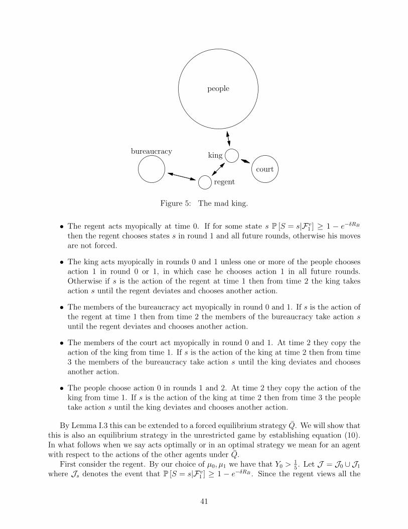
king

regent

court

bureaucracy

people

Figure 5: The mad king.

• The regent acts myopically at time 0. If for some state s P [S = s|Fv1 ] ≥ 1 − e−δRB

then the regent chooses states s in round 1 and all future rounds, otherwise his movesare not forced.

• The king acts myopically in rounds 0 and 1 unless one or more of the people choosesaction 1 in round 0 or 1, in which case he chooses action 1 in all future rounds.Otherwise if s is the action of the regent at time 1 then from time 2 the king takesaction s until the regent deviates and chooses another action.

• The members of the bureaucracy act myopically in round 0 and 1. If s is the action ofthe regent at time 1 then from time 2 the members of the bureaucracy take action suntil the regent deviates and chooses another action.

• The members of the court act myopically in round 0 and 1. At time 2 they copy theaction of the king from time 1. If s is the action of the king at time 2 then from time3 the members of the bureaucracy take action s until the king deviates and choosesanother action.

• The people choose action 0 in rounds 1 and 2. At time 2 they copy the action of theking from time 1. If s is the action of the king at time 2 then from time 3 the peopletake action s until the king deviates and chooses another action.

By Lemma I.3 this can be extended to a forced equilibrium strategy Q. We will show thatthis is also an equilibrium strategy in the unrestricted game by establishing equation (10).In what follows when we say acts optimally or in an optimal strategy we mean for an agentwith respect to the actions of the other agents under Q.

First consider the regent. By our choice of µ0, µ1 we have that Y0 >15. Let J = J0 ∪ J1

where Js denotes the event that P [S = s|Fv1 ] ≥ 1 − e−δRB . Since the regent views all the

41

myopic actions of the bureaucracy he knows the correct value of S except with probabilityexponentially small in RB so for s ∈ 0, 1, if δ > 0 is small enough,

P [Js|S = s] ≥ 1− e−δRB

and hence for large enough RB we have that Y1 ≥ 12− 2e−δRB which implies that B2 holds at

time 1. By Lemma I.5 in any optimal strategy the regent acts myopically in round 0, and sofollows the forced move. On the event Js the regent follows s in all future steps. At time 1condition B1 holds so again the regent follows the forced move in any optimal strategy. Wenext claim that for large enough RB

P[P [S = s|Fv2 ] ≥ 1− e−δRB/2

∣∣Js] = 1 (12)

Assuming (12) holds then condition B1 again holds so the regent must choose s at time 2in any optimal strategy. By construction of the forced moves from time 2 onwards the kingand bureaucracy simply imitate the regent and so he receives no further information fromtime 2 onwards. Thus again using Lemma I.5 we see that under any optimal strategy theregent must follow his forced moves.

To establish that the regent follows the forced moves in any optimal strategy it remains toshow that Condition (12) holds. The information available to the regent at time 2 includesthe actions of the king and the bureaucracy at times 0 and 1. Consider the actions ofthe bureaucracy at times 0 and 1. At time 0 they follows their initial signal. At time 1they also learn the initial action of the regent who acts myopically. By our assumptionon µ0 and µ1 that P

[Zi

0 ∈ (1, 1 + ε) ∪ (−√

7,−√

7 + ε)]

= 1, an initial signal towards 0 ismuch stronger than an initial signal towards 1, since whenever Z is negative it is at most−√

7 + ε. For i, a member of the bureaucracy, we have that Zi1 ≥ 2 if both i and the regent

choose action 1 at time 1. However, if either i or the regent choose action 0 at time 1 thenZit ≤ −

√7 + ε+ 1 + ε < −1. Since the actions of i and the regent at time 0 are known to the

regent at time 1, he gains no extra information at time 2 from his observation of i at time 1since he can correctly predict his action.

The information the regent has available at time 2 is thus his information from time 1together with the information from observing the king. The information available to theking is a function of his initial signal and that of the regent and the court. Since this is onlyRC + 1 members and we choose RB to be much larger than RC it is insignificant comparedto the information the regent observed from the court at time 0 and hence (12) holds. Thus,there is no optimal strategy for the regent that deviates from the forced moves.

As we noted above the members of the bureaucracy have |Zi0|, |Zi

1| ≥ 1 almost surely.For t ≥ 1 let Ms,t denote the event that the regent chose action s for times 1 up to t. Asargued above, Js ⊂ Ms,t for all t under Q. This analysis holds even if a single member ofthe bureaucracy adopts a different strategy as we have taken RB to be large so this changeis insignificant. Given that Ms,t holds, the only additional information available to agent i,a member of the bureaucracy, is their original signal and the action at time 1 of the regent.Thus

P[S = s

∣∣F it ,Ms,t

]≥ 1− e−δRB/2.

It follows then by Lemma I.5 that acting myopically at times 0 and 1 and then imitatingthe regent until he changes his action is the sole optimal strategy for a member of thebureaucracy.

42

Next consider the forced responses of the king. Since under Q the people always chooseaction 0 at times 0 and 1, the rule forcing the king to choose action 1 after seeing a 1 fromthe people is never invoked. We claim that, provided RB is taken to be sufficiently large,that the king acts myopically at times 0 and 1. At time 0 the posterior probability of S = 1is bounded away from 1/2 so Y0 is bounded away from 0 while 1

2− Y2 ≤ 2e−δRB/2 so by

Lemma I.5 the king must act myopically. Similarly at time 1 since our choice of µ0 and µ1 tohave their log-likelihood ratio concentrated around either 1 or −

√7 a posterior calculation

gives that,

|Zu1 −#i ∈ N(u) : Ai0(Q) = 1+

√7#i ∈ N(u) : Ai0 = 0| ≤ ε(2 +RC)

and thus for some ε(RC) > 0 sufficiently small we can find an ε′(ε, RC) > 0 such that

Y0 = | eZu1

1+eZu1− 1

2| > ε′. Since we again have that 1

2−Y1 ≤ 2e−δRB/2 taking RB = RB(ε, RC) to

be sufficiently large B2 holds and so the king must act myopically. It remains to see that theking should imitate the regent from time 2 onwards unless the regent subsequently changeshis action in any optimal strategy. This follows from a similar analysis to the case of themembers of the bureaucracy so we omit it.

We next move to an agent i, a member of the court. At time 0 the agent has Y0 >e

1+e− 1

2> 1

5. Agent i at time 1 views the action of the king who has in turn viewed the

actions of the whole court at time 0 so 12− Y2 ≤ e−cRC . At time 2 the agent sees the action

of the king who has imitated the action of the regent at time 1 so 12− Y3 ≤ e−δRB/2. Hence

provided that RC is sufficiently large and RB(RC , λ) is sufficiently large then B4 holds andi must act myopically at time 0. The information of a member of the court at time 1 isa combination of their initial signal and the action of the king at time 1. Similarly to amember of the bureaucracy, by the choice of µ0 and µ1 we have that |Zi

1| ≥ 1 and so Y0 >15.

Also 12− Y2 ≤ e−δRB/2 since this includes the information from the action of the regent at

time 1. Thus B3 holds and i must act myopically at time 1. At time 2 agents i knows theaction of the king from round 2 so Y0 ≥ 1

2− e−cRC and 1

2− Y1 ≤ e−δRB/2 so B2 holds and

i must act myopically at time 2. Finally from time 3 onwards agent i knows the action ofthe regent at time 1. As with the king and bureaucracy this will not be changed unless ireceives new information, that is the king changes his action sometime after time 2. Thusany optimal strategy of i follows the forced moves.

This finally leaves the people. Let agent i be one of the people. We first check that itis always better for them to wait and just say 0 in rounds 0 and 1 in order to get moreinformation from the king, their only source. If agent i chooses action 1 at time 0 then thetotal information it receives is a function of the initial signals of i and the king. Thus, sincethe signals are uniformly bounded, even if the agent knew the signals exactly we would havethat for some c′(µ0, µ1) that the expected utility from such a strategy is at most 1 − e−2c′ .If an agent acts with 0 at time 0 but 1 at time 1, she can potentially receive informationfrom the initial signals of the king, court and regent as well as her own; still, the optimalexpected utility even using all of this information is at most 1− e−c′(RC+3). Consider insteadthe expected utility following the forced moves. On the event J agent i will have expectedutility at least λ3(1−e−δRB) which is greater than 1−e−c′(RC+3) provided that λ is sufficientlyclose to 1 and RB is sufficiently large. Thus agent i must choose action 0 at times 0 and 1in any optimal strategy. The analysis of rounds 2 and onwards follows similarly to the courtand thus any optimal strategy of i follows all the forced moves.

43

This exhaustively shows that there is no alternative optimal strategy for any of theagents which differs from the forced moves. Thus Q is an equilibrium. However, on theevent J1 all the agents actions converge to 1. However, P [J , S = 0] ≥ e−c

′′RB > 0 wherec′′ is independent of RC , RB, λ and n. Hence, as we let n tend to infinity the probability oflearning does not tend to 1.

44