stp 421 probability lecture notes - arizona state...
TRANSCRIPT
STP 421 ProbabilityLecture Notes
Professor: John QuiggSemester: Fall 2014Revised August 11, 2014
Contents
1 Combinatorics 2
2 Probability 12
3 Conditional probability 23
4 Random variables 38
5 Continuous random variables 49
6 Jointly distributed random variables 60
7 Properties of expectation 71
Introduction
This set of notes covers the essentials of probability, using the book by Sheldon Ross as theprimary text. My intent is to keep the technical formalities to a minimum — this is a firstcourse, not an advanced one. For example, while I will occasionally give rough justificationsfor certain results, I won’t write them as formal proofs (much as I’d like to), and I won’t askyou to do proofs on exams or in homework.
1
1 COMBINATORICS 2
The Ross text has quite a lot of material — much more than we can cover in a semester.Even in the chapters we will cover, I’ll skip many things (and I’ll clearly identify whichthings are skipped). In particular, I’ll skip most of the optional sections. I want to makethis course quite basic, so that you get a good view of the forest as well as the trees. Forexample, Ross includes a large number of probability distributions, which I’ll endeavor topare down to a workable core. Also, Ross gives many elaborate examples; in general I’ll skipthe ones I deem overly fussy, concentrating instead on the more straightforward ones.
Probability has a bewildering array of applications, but in a first course such as this I preferto use “toy problems” (coin or dice tosses, card hands, balls in urns, . . . ) a lot of the time.I’ll do some applications, but I’ll try to keep those as straightforward as I can. In my opinionthis makes the techniques of probability more transparent. That said, I’ll go over many ofthe (more straightforward) examples in the book, so that we’re progressing through the booktogether.
You are expected to have a thorough working knowledge of single and multivariable calculus.But also you must be willing to deal with abstract concepts some of the time, and to do alot of problems — the only way to master the techniques of probability is to write out thedetails of many examples.
1 Combinatorics
Ross Example 2a: We have 10 women, each of whom has 3 children. How many ways canwe choose 1 of the women and 1 of her children to be mother and child of the year?
Here we need the
Multiplication Rule of Counting: The number of ways to choose 1 ball from each of rurns if the ith urn contains ni balls is
n1 · · ·nr.
Answer:
(10 ways to choose the mother) · (3 ways to choose a child of the mother) = 30.
Ross Example 2b: A college planning committee consists of 3 freshmen, 4 sophomores, 5juniors, and 2 seniors. A subcommittee of 4, consisting of 1 person from each class, is to bechosen. How many different subcommittees are possible?
1 COMBINATORICS 3
Answer:
(3 choices of freshman)·(4 choices of sophomore)·(5 choices of junior)·(2 choices of senior)
= 120.
Ross Example 2c: How many license plates are there with 3 letters followed by 4 digits?
Answer: By the Multiplication Rule, it will be
(# possibilities for the 3 letters) · (# possibilities for the 4 digits).
How to find these? Let’s do the letters: we need a special case of the Multiplication Rule,which we call
Arrangement with Repetition: The number of arrangements of k balls with repetitionfrom an urn containing n distinguishable balls is
k︷ ︸︸ ︷nn · · ·n = nk.
Notes:
• The order matters, and to emphasize this we use the word “arrange”.
• To “arrange with repetition” means we choose one of the n balls from the urn, recordthis as the 1st ball, then put it back into the urn, then choose another of the n balls,record this as the 2nd ball, etc., doing this k times.
• Another way to think of it is to imagine that we have an urn containing infinitely manyof each of n types of ball, and we choose k balls from the urn and arrange them insome order.
For the letters, we arrange 3 balls with repetition from an urn containing 26 balls, so thereare 263 possibilities. Similarly for the digits: arrange 4 balls with repetition from 10 balls.So, the answer is
263104.
Ross Example 2e: In Example 2c, what if we don’t allow repetition among the letters ornumbers?
Answer: Now we need another special case of the Multiplication Rule, which we call
1 COMBINATORICS 4
Arrangement without Repetition: The number arrangements of k balls without repeti-tion from an urn containing n balls is
k factors︷ ︸︸ ︷n(n− 1) · · · (n− k + 1) =
n!
(n− k)!.
Note: the urn has n distinguishable balls, from which we choose k balls and arrange themin some order.
For the letters, we arrange without repetition 3 balls from 26 balls, and similarly for thedigits:
(26 · 25 · 24)(10 · 9 · 8 · 7) =
(26!
23!
)(10!
6!
).
Ross Example 2d: How many functions
f : {set with n elements} → {0, 1}
are there?
Answer: 2n, because we arrange with repetition 2 balls from n balls.
Ross Example 3a: How many different batting orders are possible for a baseball teamconsisting of 9 players?
Answer: Here we use what amounts to a special case of arrangement without repetition,which we call
Permutation without Repetition: The number of arrangements of n distinct balls is
n(n− 1) · · · 1 = n!.
Notes:
• We could imagine that we have an urn containing n distinct (i.e., distinguishable) balls,and we choose all of them (without repetition) and arrange them in some order.
• We use the word “permutation” to indicate that we arrange alll of the balls. Often weomit the phrase “without repetition”, just calling it a “permutation” of n balls.
We arrange 9 balls, so we get 9!.
Ross Example 3b: A probability class, consisting of 6 men and 4 women, takes an exam,and the students are ranked according to their performance. Assume that no two students
1 COMBINATORICS 5
obtain the same score.(a) How many different rankings are possible?(b) If the men are ranked just among themselves and the women just among themselves,how many different rankings are possible?
Answer:(a) 10!, because we’re arranging 10 balls.
(b) 6! 4!, because we arrange the 6 men and the 4 women, then multiply.
Ross Example 3c: Jones has 10 books to put on her bookshelf. Of these, 4 are mathematicsbooks, 3 are chemistry books, 2 are history books, and 1 is a language book. Jones wants toarrange her books so that all the books dealing with the same subject are together on theshelf. How many different arrangements are possible?
Answer: Arrange the 4 subjects, then the books within each subject:
4! 4! 3! 2! 1!.
Ross Example 3d: How many ways can we arrange the letters PEPPER?
Answer:6!
3! 2!,
because for each of the 6! permutations of the 6 letters there are 3! permutations of the P’sand 2! permutations of the E’s that leave the arrangement unchanged.
To see the general phenomenon here, we need a variation on permutation, which we call
Permutation with Repetition: The number of arrangements of n = n1 + · · · + nk ballswhere n1 are alike, then n2 more (from the remaining n − n1) are alike, then n3 more arealike, . . . , and finally the remaining nk are alike, is(
n
n1, n2, . . . , nk
)=
n!
n1!n2! · · ·nk!.
Notes:
• Here(
nn1,n2,...,nk
)is just a shorthand notation for the fraction n!
n1!n2!···nk!.
• We also refer to the ni balls that are alike as being of “type i” (i = 1, . . . , k).
• We emphasize that we regard balls that are “alike” as identical (indistinguishable).
• The reasoning is: for each of the n! permutations of the n balls, the n1! permutationsof the balls of the 1st type, the n2! permutations of the balls of the 2nd type, . . . allleave the arrangement unchanged.
1 COMBINATORICS 6
In this example we have6 = 3 + 2 + 1
balls, where 3 are of type “P”, 2 are are of type ”E”, and the remaining 1 is of type “R”,and that’s why the answer is
6!
3! 2! 1!=
6!
3! 2!.
I want to carry this example one step further than Ross does: consider the letters AAABB.This time we have 5 = 3 + 2 balls, where 3 are alike and the 2 remaining are alike, so thenumber of arrangements is (
5
3, 2
)=
5!
3! 2!.
Once we know that there are only 2 types of ball, the decomposition n = n1+n2 is determinedby knowledge of n1 (alternatively, n2). We can form any arrangement, such as ABAAB,by choosing the 3 positions among the 5 balls for the A’s. Thus there are just as manyarrangements as there are choices of 3 out of 5 balls. In other words, we are choosinga subset (also called a “combination”) of 3 balls from a set of 5 (distinct) balls, and thenumber of these can be expressed as
5!
3!(5− 3)!.
Abstractly, we call this
Choosing: The number of ways to choose k balls (without replacement) from an urn con-taining n balls is (
n
k
)=
n!
(n− k)!k!.
Notes:
• The notation(nk
)is just a shorthand for
(n
n−k,k
).
• Unlike with arrangement without repetition, here the order does not matter, and toemphasize this we use the word “choose”. We can think of it as choosing the k ballsall at once, or one at a time but not keeping track of the order.
• We also call this the number of combinations of k things from a set of n things. In thisusage the word “combination” is a synonym for “subset”.
We’ll see more examples of this technique soon, but I just wanted to take advantage of thisopportunity to show how combinations without repetition (choosing subsets) can be relatedto permutations with repetition (arranging balls that are grouped into types).

1 COMBINATORICS 7
One more comment before we move on: we can use choosing to give another justificationthat if we have n = n1 + · · ·+ nk balls where ni balls are of type i, i = 1, . . . , k, then(
n
n1, · · · , nk
)=
n!
n1! · · ·nk!
counts the right thing: to arrange the n balls, we first choose the positions for the balls oftype 1: (
n
n1
),
then the positions for the balls of type 2, from the remaining n− n1 balls:(n− n1
n2
),
and so on, giving
# arrangements of n = n1 + · · ·+ nk balls where ni balls have type i, i = 1, . . . , k
=
(n
n1
)(n− n1
n2
)· · ·(n− n1 − n2 − · · · − nk−1
nk
).
Then canceling factorials givesn!
n1! · · ·nk!as before.
Ross Example 3e: A chess tournament has 10 competitors, of which 4 are Russian, 3 arefrom the United States, 2 are from Great Britain, and 1 is from Brazil. If the tournamentresult lists just the nationalities of the players in the order in which they placed, how manyoutcomes are possible?
Answer: We have to arrange 10 balls, grouped as 4 of type 1, 3 of type 2, 2 of type 3, and1 of type 4:
10!
4! 3! 2! 1!.
Ross Example 3f: This is similar to Example 3e.
Ross Example 4a: How many committees of 3 can be formed from 20 people?
Answer: This is “choosing”, which I introduced in a bit that I added to Example 3d: herewe are choosing 3 balls from 20 balls: (
20
3
)=
20!
17! 3!.
Ross Example 4b: From a group of 5 women and 7 men, how many different committeesconsisting of 2 women and 3 men can be formed? What if 2 of the men won’t serve together?
1 COMBINATORICS 8
Answer: For the 1st question, we choose 2 women from 5, and 3 men from 7, then multiply:(5
2
)(7
3
).
To find the number if 2 of the men can’t both be on the committee, we subtract from thetotal the number of committees that include both men. To determine a committee havingboth of the 2 men, we only need to choose the remaining 1 man from the other 5. Thus theanswer to the 2nd question is (
5
2
)(7
3
)−(
5
2
)(5
1
).
I’m skipping Ross Example 4c for now, but will solve it in Example 6d.
Ross Example 4d: Expand (x+ y)3.
Answer: When we multiply it out, we get a bunch of terms, each of which is a product ofx’s and y’s. More precisely, each term is formed by choosing either x or y from each of the3 factors in
(x+ y)3 = (x+ y)(x+ y)(x+ y),
and hence is of the form xky3−k. We want to collect the like terms, and the coefficient of eachof these terms will be the number of times it appears when we first multiply out (x + y)3.For example, the number of times x2y appears is the same as the number of ways of choosingx twice (and hence y once), in other words the # of choices of 2 balls from 3 balls, namely(32
). Putting it all together, we get:
(x+ y)3 =3∑
k=0
(3
k
)xky3−k.
This is a special case of the
Binomial Theorem: For every n ∈ {0, 1, 2, . . . },
(x+ y)n =n∑k=0
(n
k
)xkyn−k.
Due to the Binomial Theorem and its derivation,(nk
)is called the binomial coefficient n
choose k.
Ross Example 4e: How many subsets does a set with n elements have?
Answer: Let S be a set with n elements. We classify each subset of S according to howmany elements it has. For each k = 0, . . . , n, the number of subsets with k elements is
(nk
).
Thus the number of subsets of S is, by the Binomial Theorem,
n∑k=0
(n
k
)=
n∑k=0
(n
k
)1k1n−k = (1 + 1)n = 2n.
1 COMBINATORICS 9
Here is the generalization of the Binomial Theorem, with k terms instead of 2:
Multinomial Theorem: For every n ∈ {0, 1, 2, . . . } and every k ∈ N = {1, 2, 3, . . . },
(x1 + x2 + · · ·+ xk)n =
∑n1+n2+···+nk=n
(n
n1, n2, . . . , nk
)xn11 x
n22 · · ·x
nkk .
The justification is a straightforward generalization of that for the Binomial Theorem —when we multiply out the power
(x1 + x2 + · · ·+ xk)n =
n factors︷ ︸︸ ︷(x1 + x2 + · · ·+ xk) · · · (x1 + x2 + · · ·+ xk)
of the multinomial, we get terms that are products of the form
xn11 x
n22 · · ·x
nkk
where the exponents sum to n, and the number of times such a term appears is the # ofways of choosing n1 of the factors from which to pick x1, then n2 of the factors from whichto pick x2, and so on, and the total # of ways to pick x1, x2, . . . , xk is therefore
(n
n1,n2,...,nk
),
which is called a multinomial coefficient for this reason. Note that we can regard(
nn1,...,nk
)in two ways:
(1) # ways to arrange n = n1 + · · ·+ nk balls where ni balls have type i, i = 1, . . . , k;
(2) # divisions of n distinct balls into nonoverlapping subsets of sizes n1, . . . , nk.
To emphasize: in (1) we regard balls of the same type as indistinguishable, and if in (2) thesubsets are S1, . . . , Sk, then Si ∩ Sj = ∅ for all i 6= j.
Ross Example 5a: A police department in a small city consists of 10 officers. If thedepartment policy is to have 5 of the officers patrolling the streets, 2 of the officers workingfull time at the station, and 3 of the officers on reserve at the station, how many differentdivisions of the 10 officers into the 3 groups are possible?
Answer: This is permutation with repetition: we are arranging 10 balls, grouped as 5 of onetype, 2 of another type, and 3 of another type:(
10
5, 2, 3
)=
10!
5! 2! 3!.
Ross Example 5b: This is similar to Example 5a.
Ross Example 5c: In order to play a game of basketball, 10 children at a playgrounddivide themselves into two teams of 5 each. How many different divisions are possible?
1 COMBINATORICS 10
Answer: This time we are dividing a set of 10 balls into subsets of sizes 5 and 5, but thenew wrinkle is that we are not keeping track of any ordering of the 2 subsets. So, we countthe permutations with repetition of 10 balls where 5 have one type and 5 another type, thenwe divide by the number of orderings of the 2 groups:
1
2!
(10
5
)=
10!
2! 5! 5!.
Ross Example 6a: (Note that we are covering the optional section 1.6 in Ross.) How manynonnegative integer solutions (X1, X2) does the equation
X1 +X2 = 3 (1)
have?
Answer: We can regard this as the problem of distributing 3 identical balls into 2 bins.Thinking ahead to the formulation of a general technique, the trick is to first let Yi = Xi+1,and note that there are as many solutions of (1) as of
Y1 + Y2 = 5. (2)
We can regard (2) as distributing 5 balls into 2 bins, with no empty bins. Imagine that the5 identical balls are arranged as a row. We can distribute them into 2 bins by choosing 1among the 4 gaps between adjacent balls, so that the balls to the left of the gap go into the1st bin. There are (
4
1
)ways to choose the 1 gap out of 4, and this is the answer to the question. Note that(
4
1
)=
(5− 1
2− 1
)=
(2 + 3− 1
2− 1
).
Abstractly, we are distributing n+k balls into n bins, with no empty bins. This is equivalentto choosing n− 1 gaps out of n+ k − 1 gaps, and the # of ways to do this is(
n+ k − 1
n− 1
).
This is the same as counting solutions of
Y1 + Y2 + · · ·+ Yn = n+ k with Yi ∈ N, (3)
and also the same as counting solutions of
X1 +X2 + · · ·+Xn = k with Xi ∈ {0, 1, 2, . . . }. (4)
We call this

1 COMBINATORICS 11
Distribution: The number of distributions of k identical balls into n bins is(n+ k − 1
n− 1
).
Ross Example 6b: An investor has 20 thousand dollars to invest among 4 possible invest-ments. Each investment must be in units of a thousand dollars. If the total 20 thousand isto be invested, how many different investment strategies are possible? What if not all themoney need be invested?
Answer: For the 1st question, we are distributing 20 identical balls into 4 bins:(4 + 20− 1
4− 1
)=
(23
3
).
For the 2nd question, recall that the 1st question is the same as solving
X1 + · · ·+X4 = 20, Xi ∈ {0, 1, 2, . . . },
so the 2nd question is the same as solving
X1 + · · ·+X4 ≤ 20, Xi ∈ {0, 1, 2, . . . }. (5)
We can transform this into an equality by adding a “slack variable” X5, and noting that (5)has as many solutions as
X1 + · · ·+X5 = 20, Xi ∈ {0, 1, 2, . . . }.
Thus the answer is now (5 + 20− 1
5− 1
)=
(24
4
).
Ross Example 6c: How many terms are there in the multinomial expansion of (x1 + x2 +· · ·+ xr)
n? By the Multinomial Theorem, it’s the # of solutions of
n1 + · · ·+ nr = n, ni ∈ {0, 1, . . . },
which we’ve seen is (r + n− 1
r − 1
).
Ross Example 6d: (Example 4c, finally) Consider a set of n antennas of which m aredefective and n − m are functional, and assume that all of the defectives and all of thefunctionals are considered indistinguishable. How many linear orderings are there in whichno two defectives are consecutive? (I’m skipping the 2nd part of this example.)
Answer: Line up the n − m functionals. We must choose m positions for the defectivesamong the n−m− 1 gaps between the functionals and the 2 ends:(
n−m+ 1
m
).

2 PROBABILITY 12
2 Probability
We start with a random experiment (e.g., rolling two dice or dealing 5 cards).
The sample space S is the set of all possible outcomes of the experiment.
An event is any subset A ⊂ S of the sample space.
A probability on a sample space S is a function P : {events A ⊂ S} → [0, 1] such thatP (S) = 1 and P is σ-additive, i.e.,
P
(∞⋃n=1
An
)=∞∑n=1
P (An) whenever A1, A2, . . . are mutually exclusive,
meaning Ai ∩ Aj = ∅ for all i 6= j.
We think of P (A) as the fraction of the time the event A occurs in many repetitions of theexperiment.
Here’s a brief review of what we need to know about sets:
For events A,B:The union A∪B = {s : s ∈ A or s ∈ B} comprises the outcomes that are in at least one ofA or B. (Note: this allows the possibility that s ∈ A and s ∈ B.)
The intersection A ∩ B = {s : s ∈ A and s ∈ B} = {s : s ∈ A, s ∈ B} comprises theoutcomes that are in both A and B. (Note: Ross writes AB for A ∩B.)
More generally:
∞⋃i=1
Ai = {s : s ∈ Ai for at least one i}
∞⋂i=1
Ai = {s : s ∈ Ai for every i}.
The complement Ac = {s ∈ S : s /∈ A} comprises the outcomes that are not in A.
De Morgan’s Laws say that for events A1, A2, . . .(∞⋃i=1
Ai
)c
=∞⋂i=1
Aci and
(∞⋂i=1
Ai
)c
=∞⋃i=1
Aci .
And here are the elementary properties of probability:
2 PROBABILITY 13
For events A,B,P (A) = P (A ∩B) + P (A ∩Bc).
In particular,P (A) + P (Ac) = 1,
soP (Ac) = 1− P (A).
Also,
P (A ∪B) = P (A ∩Bc) + P (A ∩B) + P (B ∩ Ac) = P (A) + P (B)− P (A ∩B).
Another consequence: if A ⊂ B then P (A) ≤ P (B).
Also,P (∅) = 0.
Finally, two continuity properties:
A1 ⊂ A2 ⊂ · · · implies P
(∞⋃n=1
An
)= lim
n→∞P (An)
A1 ⊃ A2 ⊃ · · · implies P
(∞⋂n=1
An
)= lim
n→∞P (An).
Ross Example 3a:Experiment: toss a coin.Sample space: {H,T}.
P ({H}) = P ({T}) =1
2
if the coin is fair.
Ross Example 3b:Experiment: roll a die.Sample space: {1, 2, 3, 4, 5, 6}.
P ({i}) =1
6i = 1, . . . , 6
if the die is fair. So, for example,
P ({number showing is even}) = P ({2, 4, 6}) = P ({2}) + P ({4}) + P ({6}) = 3 · 1
6=
1
2.
Ross Example 4a: J is taking two books on vacation. She’ll like the 1st book withprobability .5 and the 2nd with probability .4, and both with probability .3. What’s theprobability that she likes neither book?
2 PROBABILITY 14
Answer: Define events
A = {J likes 1st book}B = {J likes 2nd book}.
We are givenP (A) = .5 and P (B) = .4.
The event that J likes both books is A ∩B, and we are given
P (A ∩B) = .3.
The event that J likes at least one book is A ∪B, and we have
P (A ∪B) = P (A) + P (B)− P (A ∩B) = .5 + .4− .3 = .6.
The event that J likes neither book is (A ∪B)c, which is
P ((A ∪B)c) = 1− P (A ∪B) = 1− .6 = .4.
The property P (A ∪B) = P (A) + P (B)− P (A ∩B) generalizes to n events:
Inclusion-Exclusion Identity: For events E1, . . . , En,
P
(n⋃i=1
Ei
)=
n∑i=1
P (Ei)−∑i<j
P (Ei ∩ Ej)
+∑i<j<k
P (Ei ∩ Ej ∩ Ek)
+ · · ·+ (−1)n+1P (E1 ∩ · · · ∩ En)
=n∑k=1
(−1)k+1∑
i1<···<ik
P
(k⋂j=1
Eij
).
Equally likely outcomes: If S is finite and P ({s}) is the same for all outcomes s, then
P (E) =#E
#Sfor every event E ⊂ S.
Ross Example 5a: If two dice are rolled, what is the probability that the sum is 7?
Answer:S = {(n, k) : n, k = 1, . . . , 6}.#S = 62 = 36.A = {sum = 7} = {(1, 6), (2, 5), . . . , (6, 1)}.
2 PROBABILITY 15
#A = 6.Thus
P (A) =6
36=
1
6.
Ross Example 5b: Choose (without replacement) 3 balls from a bowl containing 6 whiteand 5 black balls. What is the probability that one of the balls is white and the other twoare black?
Answer:S = {choices of 3 balls from 11 balls}.#S =
(113
).
A = {1 W, 2 B}.#A =
(61
)(52
).
Thus
P (A) =
(61
)(52
)(113
) .
Alternatively:S = {arrangements of 3 balls from 11 balls}.#S = 11 · 10 · 9.A = {arrangements of 1 white ball and 2 black balls}
#A =(6 choices of 1 W)·(5 choices of 1st B)·(4 choices of 2nd B)·(3 choices of slot for W).
So
P (A) =6 · 5 · 4 · 311 · 10 · 9
.
There’s apparently a second part to this example: we choose 5 people from 10 marriedcouples. What’s the probability that all 5 come from distinct couples?
Answer:S = {choices of 5 people from 20}#S =
(205
).
Let A = {sets of 5 people from distinct couples}. Then
#A =
((10
5
)choices of 5 couples
)·(25 choices of 1 member of each couple
).
Thus
P (A) =
(105
)25(
205
) .

2 PROBABILITY 16
Again, Ross gives an alternative solution using arrangements rather than sets.
Ross Example 5c: A committee of 5 is to be selected from 6 men and 9 women. What isthe probability that the committee has 3 men and 2 women?
Answer:S = {choices of 5 from 15}.#S =
(155
).
A = {3 men, 2 women}.#A =
(63
)(92
).
Thus
P (A) =
(63
)(92
)(155
) .
Ross Example 5d: An urn contains n balls, one of which is special. Choose k of theseballs (without replacement). What’s the probability that the special ball is chosen?
Answer:S = {choices of k balls from n balls}.#S =
(nk
).
A = {special ball and k − 1 other balls}.#A =
(11
)(n−1k−1
).
Thus
P (A) =
(11
)(n−1k−1
)(nk
) .
Alternatively:S = {arrangements of k balls from n distinct balls}.#S = n(n− 1) · · · (n− k + 1).A = {special ball is chosen}.For each i = 1, . . . , k let Ai = {ith ball chosen is special}. Then #Ai = #A1. It might seemobvious that P (A1) = 1/n, but let’s give a convincing argument:A1 = {(special ball)b2 . . . bk : b2, . . . , bk nonspecial balls}.#A = (n− 1)(n− 2) · · · (n− k + 1).Thus
P (A1) =(n− 1)(n− 2) · · · (n− k + 1)
n(n− 1) · · · (n− k + 1)=
1
n.
Since A1, . . . , Ak are mutually exclusive and A =⋃ki=1Ai,
P (A) =k∑i=1
P (Ai) =k
n.
Note that part of the above solution shows
P (Ai) = P (A1) = P (any particular ball when 1 ball is chosen) =1
n.
2 PROBABILITY 17
This observation will be useful later.
Ross Example 5e: Suppose we consider all arrangements of n red balls and m blue balls.If we regard balls of the same color as identical (indistinguishable), we want to convinceourselves that all arrangements are equally likely, and it goes like this: suppose temporarilythat we can distinguish balls of the same color, so we have a set
B = {r1, . . . , rn, b1, . . . , bm},
which has (n + m)! permutations. On the other hand, when balls of the same color areregarded as identical, each arrangement is just an arrangement of the letters
n︷ ︸︸ ︷rr · · · r
m︷ ︸︸ ︷bb · · · b,
and there are(n+mn
)of these. Each arrangement of the letters corresponds to n!m! permu-
tations of B, and this is why the arrangements are equally likely.
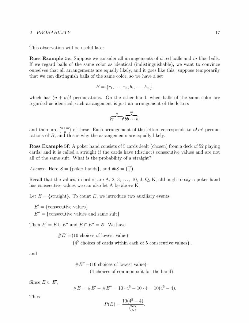
Ross Example 5f: A poker hand consists of 5 cards dealt (chosen) from a deck of 52 playingcards, and it is called a straight if the cards have (distinct) consecutive values and are notall of the same suit. What is the probability of a straight?
Answer: Here S = {poker hands}, and #S =(525
).
Recall that the values, in order, are A, 2, 3, . . . , 10, J, Q, K, although to say a poker handhas consecutive values we can also let A be above K.
Let E = {straight}. To count E, we introduce two auxiliary events:
E ′ = {consecutive values}E ′′ = {consecutive values and same suit}
Then E ′ = E ∪ E ′′ and E ∩ E ′′ = ∅. We have
#E ′ =(10 choices of lowest value)·(45 choices of cards within each of 5 consecutive values
),
and
#E ′′ =(10 choices of lowest value)·(4 choices of common suit for the hand).
Since E ⊂ E ′,#E = #E ′ −#E ′′ = 10 · 45 − 10 · 4 = 10(45 − 4).
Thus
P (E) =10(45 − 4)(
525
) .
2 PROBABILITY 18
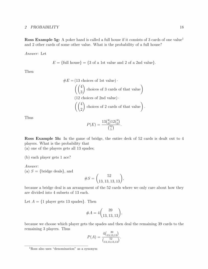
Ross Example 5g: A poker hand is called a full house if it consists of 3 cards of one value1
and 2 other cards of some other value. What is the probability of a full house?
Answer: Let
E = {full house} = {3 of a 1st value and 2 of a 2nd value}.
Then
#E = (13 choices of 1st value) ·((4
3
)choices of 3 cards of that value
)(12 choices of 2nd value) ·((
4
2
)choices of 2 cards of that value
).
Thus
P (E) =13(43
)12(42
)(525
) .
Ross Example 5h: In the game of bridge, the entire deck of 52 cards is dealt out to 4players. What is the probability that(a) one of the players gets all 13 spades;
(b) each player gets 1 ace?
Answer:(a) S = {bridge deals}, and
#S =
(52
13, 13, 13, 13
),
because a bridge deal is an arrangement of the 52 cards where we only care about how theyare divided into 4 subsets of 13 each.
Let A = {1 player gets 13 spades}. Then
#A = 4
(39
13, 13, 13
),
because we choose which player gets the spades and then deal the remaining 39 cards to theremaining 3 players. Thus
P (A) =4(
3913,13,13
)(52
13,13,13,13
) .1Ross also uses “denomination” as a synonym

2 PROBABILITY 19
Ross has an alternative solution: let Ai = {player i gets all the spades}. Similarly to ourobservation at the end of Ross Example 5d, since getting all the spades is one particularbridge hand,
P (Ai) = P (A1) = P ({any particular bridge hand} =1(5213
) .Since A = A1 ∪ · · · ∪ A4 and the Ai’s are mutually exclusive,
P (A) = 4P (A1) =4(5213
) .It’s routine to check that our 2 answers agree.
(b) Let B = {each player gets 1 ace}. Then
#B = 4!
(48
12, 12, 12, 12
)because we distribute the 4 aces among the players, then deal the remaining 48 cards. Thus
P (B) =4!(
4812,12,12,12
)(52
13,13,13,13
) .Ross Example 5i: (Birthday Problem) Among n people, what is the probability that notwo have a birthday on the same day of the year?
Answer: Ignoring leap years, a birthday is any integer from 1 to 365. Let
S = {arrangements of n birthdays}= {arrangements of n balls each of which can be of 365 types}.
so that#S = 365n.
Let
A = {no 2 have the same birthday} = {arrangements of n balls from a set of 365},
so that#A = 365 · 364 · 363 · · · (365− n+ 1).
Then
P (A) =365 · 364 · 363 · · · (365− n+ 1)
365n.
Ross Example 5j: Cards are turned up one at a time from a shuffled deck of 52 playingcards until the first ace appears. Is the next card — that is, the card following the first ace— more likely to be the ace of spades or the two of clubs?
2 PROBABILITY 20
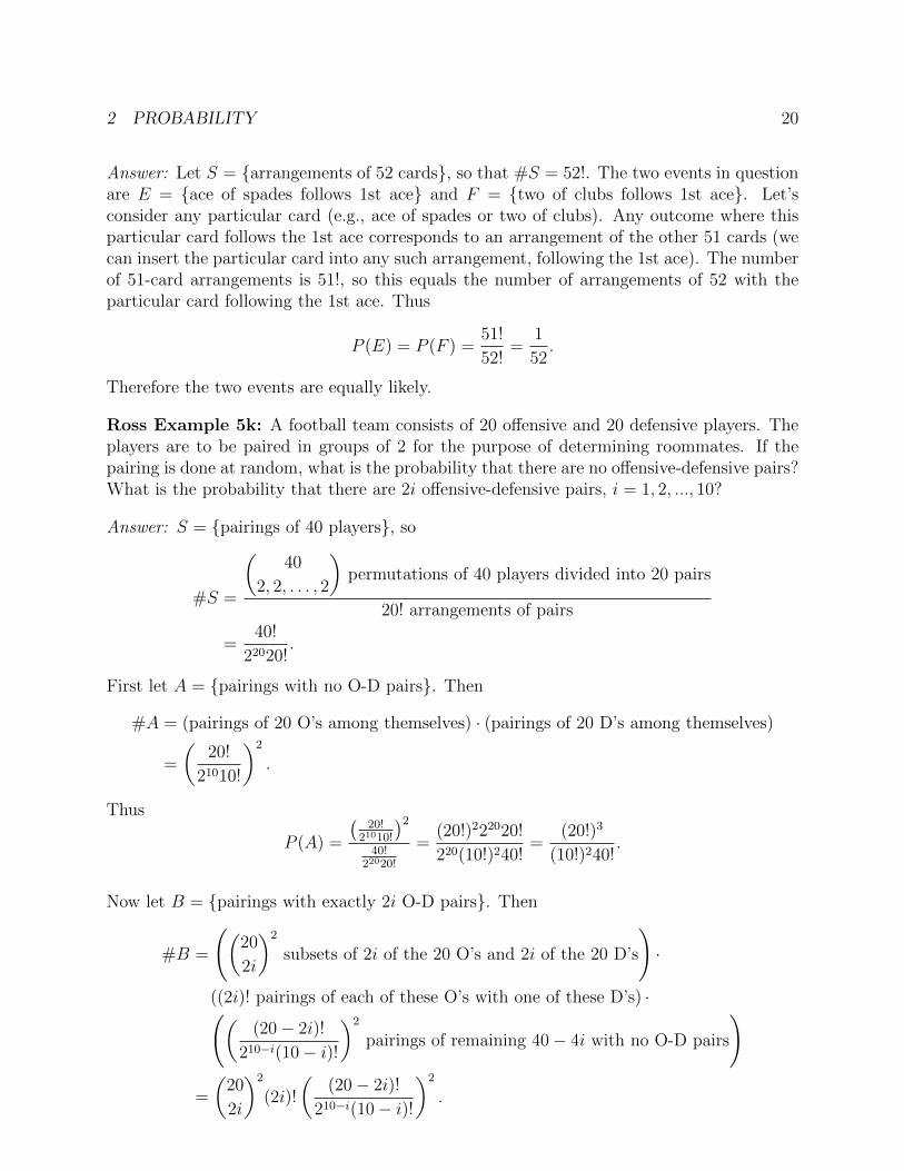
Answer: Let S = {arrangements of 52 cards}, so that #S = 52!. The two events in questionare E = {ace of spades follows 1st ace} and F = {two of clubs follows 1st ace}. Let’sconsider any particular card (e.g., ace of spades or two of clubs). Any outcome where thisparticular card follows the 1st ace corresponds to an arrangement of the other 51 cards (wecan insert the particular card into any such arrangement, following the 1st ace). The numberof 51-card arrangements is 51!, so this equals the number of arrangements of 52 with theparticular card following the 1st ace. Thus
P (E) = P (F ) =51!
52!=
1
52.
Therefore the two events are equally likely.
Ross Example 5k: A football team consists of 20 offensive and 20 defensive players. Theplayers are to be paired in groups of 2 for the purpose of determining roommates. If thepairing is done at random, what is the probability that there are no offensive-defensive pairs?What is the probability that there are 2i offensive-defensive pairs, i = 1, 2, ..., 10?
Answer: S = {pairings of 40 players}, so
#S =
(40
2, 2, . . . , 2
)permutations of 40 players divided into 20 pairs
20! arrangements of pairs
=40!
22020!.
First let A = {pairings with no O-D pairs}. Then
#A = (pairings of 20 O’s among themselves) · (pairings of 20 D’s among themselves)
=
(20!
21010!
)2
.
Thus
P (A) =
(20!
21010!
)240!
22020!
=(20!)222020!
220(10!)240!=
(20!)3
(10!)240!.
Now let B = {pairings with exactly 2i O-D pairs}. Then
#B =
((20
2i
)2
subsets of 2i of the 20 O’s and 2i of the 20 D’s
)·
((2i)! pairings of each of these O’s with one of these D’s) ·(((20− 2i)!
210−i(10− i)!
)2
pairings of remaining 40− 4i with no O-D pairs
)
=
(20
2i
)2
(2i)!
((20− 2i)!
210−i(10− i)!
)2
.

2 PROBABILITY 21
Thus
P (B) =
(202i
)2(2i)!
((20−2i)!
210−i(10−i)!
)240!
22020!
.
Ross Example 5l: (Inclusion-Exclusion) 36 members of a club play tennis, 28 play squash,and 18 play badminton. Furthermore, 22 of the members play both tennis and squash, 12play both tennis and badminton, 9 play both squash and badminton, and 4 play all threesports. How many members of this club play at least one of three sports?
Answer: Let
A = {tennis players}B = {squash players}C = {badminton players}.
We need a combinatorial analog of the Inclusion-Exclusion Identity from probability, butwe’ll only state it for 3 sets, since that’s what we need here:
#(A ∪B ∪ C) = #A+ #B + #C
−#(A ∩B)−#(A ∩ C)−#(B ∩ C)
+ #(A ∩B ∩ C)
= 36 + 28 + 18− 22− 12− 9 + 4
= 43.
Note: Ross solves this using probabilities directly; the two solutions are essentially the same.
Ross Example 5m: (Matching Problem) Each of N men throws his hat into a pile. Thehats are mixed up and each man randomly selects a hat from the pile. What’s the probabilitythat none of the men selects his own hat?
Answer: S = {pairings of men with hats}, so #S = N !. Let A = {no man gets own hat}.Also let Ai = {ith man gets own hat}, i = 1, . . . , N . Then
Ac = at least 1 man gets own hat =N⋃i=1
Ai.
Thus, by the Inclusion-Exclusion Identity,
P (A) = 1− P (Ac)
= 1− P
(N⋃i=1
Ai
)
= 1−N∑k=1
(−1)k+1∑
i1<···<ik
P
(k⋂j=1
Aij
).
2 PROBABILITY 22
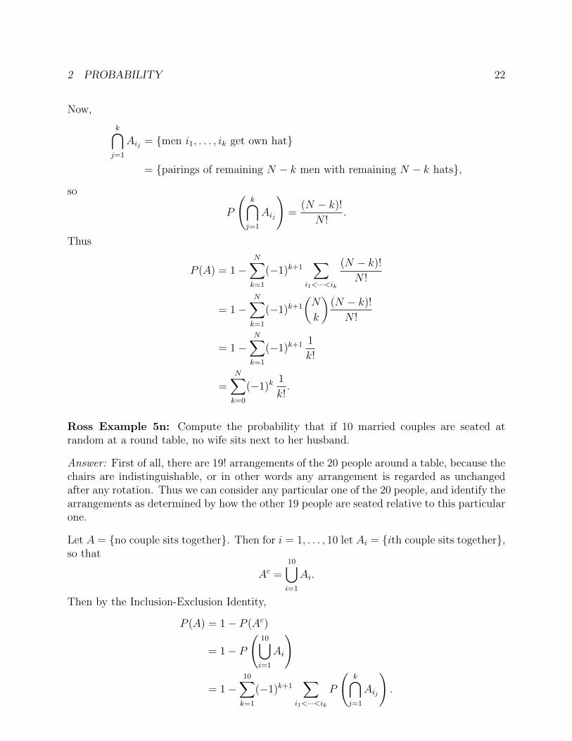
Now,
k⋂j=1
Aij = {men i1, . . . , ik get own hat}
= {pairings of remaining N − k men with remaining N − k hats},
so
P
(k⋂j=1
Aij
)=
(N − k)!
N !.
Thus
P (A) = 1−N∑k=1
(−1)k+1∑
i1<···<ik
(N − k)!
N !
= 1−N∑k=1
(−1)k+1
(N
k
)(N − k)!
N !
= 1−N∑k=1
(−1)k+1 1
k!
=N∑k=0
(−1)k1
k!.
Ross Example 5n: Compute the probability that if 10 married couples are seated atrandom at a round table, no wife sits next to her husband.
Answer: First of all, there are 19! arrangements of the 20 people around a table, because thechairs are indistinguishable, or in other words any arrangement is regarded as unchangedafter any rotation. Thus we can consider any particular one of the 20 people, and identify thearrangements as determined by how the other 19 people are seated relative to this particularone.
Let A = {no couple sits together}. Then for i = 1, . . . , 10 let Ai = {ith couple sits together},so that
Ac =10⋃i=1
Ai.
Then by the Inclusion-Exclusion Identity,
P (A) = 1− P (Ac)
= 1− P
(10⋃i=1
Ai
)
= 1−10∑k=1
(−1)k+1∑
i1<···<ik
P
(k⋂j=1
Aij
).
3 CONDITIONAL PROBABILITY 23
Now,
k⋂j=1
Aij = {couples i1, . . . , ik sit together},
and each of these outcomes can be formed by first grouping couples i1, . . . , ik into k blocksof size 2, then arranging these k blocks and the remaining 20− 2k people around the table,and then arranging the members within each of the k couples, so
#k⋂j=1
Aij = (k + 20− 2k − 1)!(2!)k = (19− k)!2k.
Thus
P
(k⋂j=1
Aij
)=
(19− k)!2k
19!.
Therefore
P (A) = 1−10∑k=1
(−1)k+1∑
i1<···<ik
(19− k)!2k
19!
= 1−10∑k=1
(−1)k+1
(10
k
)(19− k)!2k
19!
=10∑k=0
(−1)k(
10
k
)(19− k)!2k
19!.
I’m skipping the rest of Ross Chapter 2.
3 Conditional probability
If A and B are events with P (B) > 0, the conditional probability of A given B is
P (A|B) =P (A ∩B)
P (B).
Ross Example 2a: Joe is 80% certain that his missing key is in one of the two pockets ofhis jacket, being 40% certain it’s in the left-hand pocket, and 40% certain it’s in the right-hand pocket. If a search of the left-hand pocket doesn’t find the key, what’s the conditionalprobability that it’s in the other pocket?
3 CONDITIONAL PROBABILITY 24
Answer: Let
A = {key is in left-hand pocket}B = {key is in right-hand pocket}.
Then
P (B|Ac) =P (B ∩ Ac)P (Ac)
=P (B)
1− P (A)(A and B are mutually exclusive)
=.4
1− .4
=2
3.
Ross Example 2b: Toss a coin twice. What is the conditional probability that both tossesare heads, given(a) the first toss is heads?
(b) at least one toss is heads?
Answer: First we’ll do it using the definition of conditional probability: The sample spaceis S = {HH,HT, TH, TT}. Let
A = {both H} = {HH}.
(a) LetB = {1st is H} = {HH,HT}.
Then
P (A|B) =P (A ∩B)
P (B)=P (A)
P (B)(because A ⊂ B)
=1/4
1/2=
1
2.
(b) LetC = {at least 1 H} = {HH,HT, TH}.
Then
P (A|C) =P (A ∩ C)
P (C)=P (A)
P (C)(because A ⊂ C)
=1/4
3/4=
1
3.

3 CONDITIONAL PROBABILITY 25
Now we’ll solve it using the reduced sample space: abstractly, an event F ⊂ S becomesa sample space, with probability P (·|F ) given by
P (E|F ) =P (E)
P (F )for E ⊂ F.
When the original sample space S has equally likely outcomes, so does the reduced samplespace F , so for E ⊂ F we have
P (E|F ) =#E
#F.
(a) Since S has equally likely outcomes, so does any reduced sample space. Here we haveA ⊂ B, #A = 1, and #B = 2, so
P (A|B) =1
2.
(b) Here A ⊂ C, #A = 1, and #C = 3, so
P (A|C) =1
3.
Ross Example 2c: In bridge, the 52 cards are dealt out equally to 4 players — called East,West, North, and South. If North and South have a total of 8 spades among them, what isthe probability that East has 3 of the remaining 5 spades?
Answer: In this example, we can ignore West, and we concentrate on the reduced samplespace B, in which 26 cards have already been dealt to North and South. Since the originalsample space has equally likely outcomes, so does B. We are interested in the 13 cardsdealt to East from the remaining 26. We know that these remaining 26 cards contain only 5spades. So, we have 26 cards of which 5 are spades, and the reduced sample space B is allchoices of 13 of these 26, so #B =
(2613
). Let A = {3 spades}. Then #A =
(53
)(2110
), so
P (A) =
(53
)(2110
)(2613
) .
Ross Example 2d: Celine is undecided as to whether to take a French course or a chemistrycourse. She estimates that her probability of receiving an A grade would be 1/2 in a Frenchcourse and 2/3 in a chemistry course. If Celine decides to base her decision on the flip of afair coin, what is the probability that she gets an A in chemistry?
Answer: Let
C = {Celine chooses Chemistry}A = {Celine gets an A},

3 CONDITIONAL PROBABILITY 26
so that A ∩ C = {Celine gets an A in Chemistry}. The choice is determined by a fair coin,so
P (C) =1
2,
and we are given
P (A|C) =2
3.
Thus
P (A ∩ C) = P (A|C)P (C) =2
3· 1
2=
1
3.
Ross Example 2e: Suppose that an urn contains 8 red balls and 4 white balls. We draw(choose) 2 balls from the urn without replacement.(a) If we assume that at each draw each ball in the urn is equally likely to be chosen, whatis the probability that both balls drawn are red?
(b) Now suppose that the balls have different weights, with each red ball having weight r andeach white ball having weight w. Suppose that the probability that a given ball in the urnis the next one selected is its weight divided by the sum of the weights of all balls currentlyin the urn. Now what is the probability that both balls are red?
Answer:(a) Let A = {both red}. We are choosing 2 balls from 12, with equally likely outcomes, so
P (A) =
(82
)(122
) .Alternatively, we can let
S = {arrangements of 2 balls from 12}A1 = {1st ball red}A2 = {2nd ball red},
and then compute
P (A) = P (A1 ∩ A2) = P (A1)P (A2|A1) =
(8
12
)(7
11
).
(b) This time we only give one method, taking the order into account. We consider the redballs individually. Let
Ei = {1st ball drawn is ith red ball} i = 1, . . . , 8,
so thatP (Ei) =
r
8r + 4w.

3 CONDITIONAL PROBABILITY 27
Then
A1 =8⋃i=1
Ei,
and the Ei’s are mutually exclusive, so
P (A1) =8∑i=1
P (Ei) =8r
8r + 4w.
Similarly,
P (A2|A1) =7r
7r + 4w.
Thus
P (A) = P (A1)P (A2|A1) =
(8r
8r + 4w
)(7r
7r + 4w
)The use of conditional probability to handle intersection generalizes:
P (E1 ∩ · · · ∩ En) = P (E1)P (E1 ∩ E2)
P (E1)
P (E1 ∩ E2 ∩ E3)
P (E1 ∩ E2)· · · P (E1 ∩ · · · ∩ En)
P (E1 ∩ · · · ∩ En−1)= P (E1)P (E2|E1)P (E3|E1 ∩ E2) · · ·P (En|E1 ∩ · · · ∩ En−1).
Ross Example 2f: (Matching Problem again) In the matching problem stated in Example5m of Chapter 2, it was shown that the probability PN that there are no matches when Npeople randomly select from among their own N hats, is given by
PN =N∑i=0
(−1)i
i!.
What is the probability that exactly k of the N people have matches?
Answer: (Instructor comment: here Ross uses “select from among their own hats” to mean“select from the pile of hats” — the phrase “their own” here could be confusing.) Any twosubsets of k people are equally likely to be exactly the people who match, so let’s focus onpeople 1, . . . , k. Let
Ei = {ith person matches}F = {none of persons k + 1, . . . , n matches}.
We are interested in E1 ∩ · · · ∩ Ek ∩ F :
P (E1 ∩ · · · ∩ Ek ∩ F )
= P (E1)P (E2|E1)P (E3|E1 ∩ E2) · · ·P (Ek|E1 ∩ · · · ∩ Ek−1)· P (F |E1 ∩ · · · ∩ Ek)
=1
N
1
N − 1
1
N − 2. . .
1
N − k + 1
N−k∑i=0
(−1)i
i!,
3 CONDITIONAL PROBABILITY 28
so
P (exactly k matches)
=∑
i1<···<ik
P (people i1, . . . , ik match, none of the other N − k match)
=
(N
k
)P (E1 ∩ · · · ∩ Ek ∩ F )
=
(N
k
)1
N
1
N − 1
1
N − 2. . .
1
N − k + 1
N−k∑i=0
(−1)i
i!
=1
k!
N−k∑i=0
(−1)i
i!.
Ross Example 2g: A deck of 52 playing cards is randomly divided into 4 piles of 13 cardseach. Compute the probability that each pile has exactly 1 ace.
Answer: We already solved this without conditional probability, in Ross Chapter 2, Example5h. Ross gives a clever solution here using conditional probability, but I’ll give a morestraightforward solution, which Ross hints at in Problem 13.
Let Ei = {ith player gets exactly 1 ace}, i = 1, . . . , 4. Then
P (E1 ∩ · · · ∩ E4) = P (E1)P (E2|E1)P (E3|E1 ∩ E2)P (E4|E1 ∩ E2 ∩ E3)
=
(41
)(4812
)(5213
) · (31)(3612)(3913
) · (21)(2412)(2613
) · 1To see this, note that P (E1) is clear. Given E1, there are 39 cards left, of which 3 are aces,so now P (E2|E1) is clear, and similarly for P (E3|E1∩E2). Finally, given E1∩E2∩E3, thereis 1 ace left in the remaining 13 cards, so player 4 must get it. It’s routine to check that thisanswer agrees with our earlier one, and with Ross’.
Bayes’ Rule: If B1, . . . , Bn form a partition of S, then
P (Bj|A) =P (Bj ∩ A)
P (A)=
P (A|Bj)P (Bj)∑ni=1 P (A|Bi)P (Bi)
.
Justification:
P (A) =n∑i=1
P (A ∩Bi) =n∑i=1
P (A|Bi)P (Bi),
Ross Example 3a:(Part I) An insurance company believes that people can be divided into two classes: thosewho are accident prone and those who are not. The company’s statistics show that anaccident-prone person will have an accident at some time within a fixed 1-year period with
3 CONDITIONAL PROBABILITY 29
probability .4, whereas this probability decreases to .2 for a person who is not accident prone.If we assume that 30 percent of the population is accident prone, what is the probabilitythat a new policyholder will have an accident within a year of purchasing a policy?
Answer: Let
A = {accident-prone}B = {has accident in a year}.
ThenP (B) = P (B|A)P (A) + P (B|Ac)P (Ac) = .4(.3) + .2(.7) = .26.
(Part II) Suppose that a new policyholder has an accident within a year of purchasing apolicy. What is the probability that he or she is accident prone?
Answer:
P (A|B) =P (B|A)P (A)
P (B)=.4(.3)
.26=
6
13.
I’m skipping Ross Example 3b.
Ross Example 3c: In answering a question on a multiple-choice test, a student eitherknows the answer or guesses. Let p be the probability that the student knows the answerand 1 − p be the probability that the student guesses. Assume that a student who guessesat the answer will be correct with probability 1/m, where m is the number of multiple-choice alternatives. What is the conditional probability that a student knew the answer toa question given that he or she answered it correctly?
Answer: Let
K = {student knew answer}C = {student answered correctly}.
Then by Bayes’ Rule
P (K|C) =P (C|K)P (K)
P (C|K)P (K) + P (C|Kc)P (Kc)
=1 · p
1 · p+ (1/m)(1− p)=
mp
1 + (m− 1)p.
Ross Example 3d: A laboratory blood test is 95 percent effective in detecting a certaindisease when it is, in fact, present. However, the test also yields a “false positive” result for1 percent of the healthy persons tested. (That is, if a healthy person is tested, then, withprobability .01, the test result will indicate that he or she has the disease.) If .5 percent of
3 CONDITIONAL PROBABILITY 30
the population actually has the disease, what is the probability that a person has the diseasegiven that the test result is positive?
Answer: Let
D = {has disease}T = {test positive}.
Then by Bayes’ Rule
P (D|T ) =P (T |D)P (D)
P (T |D)P (D) + P (T |Dc)P (Dc)
=.95(.005)
.95(.005) + .01(.995).
I’m skipping Ross Examples 3e–3f, and “odds”.
Ross Example 3i: An urn contains two type A coins and one type B coin. When a typeA coin is flipped, it comes up heads with probability 1/4, whereas when a type B coin isflipped, it comes up heads with probability 3/4. A coin is randomly chosen from the urnand flipped. Given that the flip landed on heads, what is the probability that it was a typeA coin?
Answer: Let
A = {type A coin}B = {type B coin}H = {heads}.
Then
P (A|H) =P (H|A)P (A)
P (H|A)P (A) + P (H|Ac)P (Ac)
=14· 23
14· 23
+ 34· 13
=2
5.
I’m skipping Ross Examples 3j–3k.
Ross Example 3l: We have 3 cards. The 1st card is red on both sides, the 2nd is blackon both sides, and the 3rd is red on one side and black on the other. We choose 1 card andlook at one side. If it’s red, what’s the probability that the other side is black?
3 CONDITIONAL PROBABILITY 31
Answer: Let
A = {side showing is red}Ci = {card i}, i = 1, 2, 3.
Then
P (other side black|A) = P (C3|A) (reduced sample space)
=P (A|C3)P (C3)∑3i=1 P (A|Ci)P (Ci)
=(1/2)(1/3)
1(1/3) + 0(1/3) + (1/2)(1/3)
=1
3.
I’m skipping Ross Examples 3m–3o.
Events A and B are independent if
P (A ∩B) = P (A)P (B),
otherwise they are dependent. If P (B) > 0, independence is equivalent to
P (A|B) = P (A),
and similarly if P (A) > 0.
Ross Example 4a: Deal a card from a deck. Then
E = {ace} and F = {spade}
are independent, because
P (E)P (F ) =1
13· 1
4=
1
52= P (E ∩ F ).
Ross Example 4b: Toss 2 coins. Then
E = {1st is H} = {HH,HT} and F = {2nd is T} = {HT, TT}
are independent, because
P (E)P (F ) = P ({HH,HT})P ({HT, TT}) =1
2· 1
2=
1
4= P ({HT}) = P (E ∩ F ).
Ross Example 4c: Roll 2 dice. Let
E1 = {sum = 6} = {(1, 5), . . . , (5, 1)}E2 = {sum = 7} = {(1, 6), . . . , (6, 1)}F = {1st is 4} = {(4, 1), . . . , (4, 6)}.

3 CONDITIONAL PROBABILITY 32
Then
P (E1)P (F ) =5
36· 1
6,
while
P (E1 ∩ F ) = P ({(4, 2)}) =1
36,
so E1 and F are dependent.
On the other hand,
P (E2)P (F ) =6
36· 1
6=
1
36,
while
P (E2 ∩ F ) = P ({(4, 3)}) =1
36,
so E2 and F are independent.
Alternatively,
P (E1|F ) = P ({(4, 2)}) =1
66= 5
36= P (E1),
while
P (E2|F ) = P ({(4, 3)}) =1
36= P (E2),
showing that F is independent of E2 but not E1.
I’m skipping 4d.
Generalizing: E1, . . . , En are independent if
P (Ei1 ∩ · · · ∩ Eik) = P (Ei1) · · ·P (Eik) for all i1 < · · · < ik,
otherwise they are dependent. An infinite sequence E1, E2, . . . is independent if any finitesubset is independent, and dependent otherwise.
It is not hard to see that if E1, . . . , En are independent then so are any combination (unions,intersections, complements) of E1, . . . , Ek and any combination of Ek+1, . . . , En.
Ross Example 4e: Roll 2 dice. Let
E = {sum = 7}F = {1st = 4}G = {2nd = 3}.
Then
P (E|F ∩G) = 1 6= 1
6= P (E),
so E,F,G are dependent.
3 CONDITIONAL PROBABILITY 33
A sequence of experiments is called independent if any sequence E1, E2, . . . of events isindependent provided Ei depends only on the outcome of the ith experiment, i = 1, 2, . . . .
If all the sample spaces are equal, we call the experiments trials.
Ross Example 4f: Consider a sequence of independent trials, in which each trial results in“success” with probability p (and “failure” = successc). What’s the probability that(a) at least 1 success occurs in the first n trials;
(b) exactly k successes occur in the first n trials;
(c) all trials result in successes?
Answer:(a)
P (≥ 1 success in 1st n trials) = 1− P (all failures in 1st n trials)
= 1− (1− p)n (by independence of trials).
(b)
P (exactly k successes in 1st n trials) =
(n
k
)pk(1− p)n−k,
because we have to choose the k trials out of n trials for the successes, and the probabilityof any such choice is pk(1− p)n−k by independence.
(c) Let
E = {all successes}En = {all success in 1st n trials}, n = 1, 2, . . . .
ThenE1 ⊃ E2 ⊃ · · ·
and∞⋂n=1
En = E,
so by continuity of probability we have
P (E) = limn→∞
P (En).
We have P (En) = pn, so
P (E) = limn→∞
pn =
{0 if p < 1
1 if p = 1.
3 CONDITIONAL PROBABILITY 34
I’m skipping Ross Example 4g.
Ross Example 4h: Consider a sequence of independent trials of rolling 2 dice. What’s theprobability of that a sum of 5 appears before a sum of 7?
Answer: Let
A = {5 before 7}An = {5 on nth roll, neither 5 nor 7 before}.
On any single roll,
P (5) =1
9and P (7) =
1
6,
so, because 5 and 7 are mutually exclusive,
P (5 or 7) =1
9+
1
6=
5
18,
and hence
P (neither 5 nor 7) = 1− 5
18=
13
18.
By independence,
P (An) =
(13
18
)n−11
9.
We have A =⋃∞n=1An, so, because the An’s are mutually exclusive,
P (A) =∞∑n=1
P (An) =∞∑n=1
(13
18
)n−11
9=
1/9
1− 13/18=
2
5.
Alternative solution (which is useful in Chapter 3 Problem 76): condition on the outcomeof the 1st roll. Let
E = {sum = 5 on 1st roll}F = {sum = 7 on 1st roll}G = {sum is neither 5 nor 7 on 1st roll}.
Then E,F,G form a partition of the sample space {(n, k) : n, k = 1, . . . , 6}, and
P (G) = 1− P (E)− P (F ) = 1− 4
36− 6
36=
26
36.
If G occurs on the 1st roll, then we are starting again with the same conditions, so P (A|G) =P (A). Thus
P (A) = P (A|E)P (E) + P (A|F )P (F ) + P (A|G)P (G)
= 1 ·(
4
36
)+ 0 ·
(6
36
)+ P (A)
(26
36
)=
4
36+
26P (A)
36,
3 CONDITIONAL PROBABILITY 35
and solving for P (A) we get
P (A) =4
10=
2
5.
Ross Example 4i: (Coupon collecting) There are n types of coupons, and each new onecollected is independently of type i with probability pi (so that
∑ni=1 pi = 1). We collect k
coupons. Let Ai = {at least type one i coupon is collected}. For i 6= j find:(a) P (Ai)
(b) P (Ai ∪ Aj)
(c) P (Ai|Aj)
Answer:(a)
P (Ai) = 1− P (Aci)
= 1− (1− pi)k (by independence) .
(b)
P (Ai ∪ Aj) = 1− P ((Ai ∪ Aj)c)= 1− P (Aci ∩ Acj)= 1− (1− pi − pj)k.
(c) Note that
P (Ai ∩ Aj) = P (Ai) + P (Aj)− P (Ai ∩ Aj)= 1− (1− pi)k + 1− (1− pj)k −
(1− (1− pi − pj)k
)= 1− (1− pi)k − (1− pj)k + (1− pi − pj)k.
Thus
P (Ai|Aj) =P (Ai ∩ Aj)P (Aj)
=1− (1− pi)k − (1− pj)k + (1− pi − pj)k
1− (1− pj)k.
Ross Example 4j: (Problem of the Points) Consider independent trials resulting in successwith probability p and failure with probability 1−p. What’s the probability that n successesoccur before m failures?
Answer: The event is
A = {at least n successes in 1st n+m− 1 trials}.
3 CONDITIONAL PROBABILITY 36
For every k letAk = {exactly k success in 1st n+m− 1 trials}.
Then
A =n+m−1⋃k=n
Ak
and the Ak’s are mutually exclusive, so
P (A) =n+m−1∑k=n
P (Ak) =n+m−1∑k=n
(n+m− 1
k
)pk(1− p)n+m−1−k.
I’m skipping Ross Example 4k-4l.
Ross Example 4m: (Gambler’s Ruin) (Instructor comment: I’m reducing the examplefrom what Ross presents.)
Let 0 < i < 10 and 0 < p < 1. Suppose we start with i dollars. In each round of a gamewe either win a dollar with probability p or lose a dollar with probability 1− p, and we playuntil we either get to 10 dollars, in which case we win the game, or to 0 dollars, in which welose the game. Let Pi = P (we win the game). Show that
Pi+1 − Pi =1− pp
(Pi − Pi−1
).
Answer: Let R be the event that we win the first round, in which case we are then playingthe game starting with i+ 1 dollars, and similarly for Rc. Thus
Pi = P (Ei|R)P (R) + P (Ei|Rc)P (Rc) = Pi+1p+ Pi−1(1− p).
Writing Pi = pPi + (1− p)Pi, we can rearrange to get
(1− p)(Pi − Pi−1) = p(Pi+1 − Pi),
and we can solve for Pi+1 − Pi.
In preparation for the next example, note that it is not hard to see that for any fixed eventB the function
P (·|B) : {events} → [0, 1]
is a probability.
Ross Example 5a: Revisiting Ross Chapter 3 Example 3a: in any given year, an accident-prone person will have an accident with probability .4, whereas the probability for a non-accident-prone person is .2. What’s the conditional probability of an accident in the 2ndyear, given an accident in the 1st year?
3 CONDITIONAL PROBABILITY 37
Answer: Let
A = {accident-prone}Bi = {accident in ith year}.
We want P (B2|B1). Define a probability Q by
Q(E) = P (E|B1).
We saw in Ross Chapter 3 Example 3a that P (B1) = .26. We have
P (B2|B1) = Q(B2)
= Q(B2|A)Q(A) +Q(B2|Ac)Q(Ac).
Now,
Q(B2|A) =Q(B2 ∩ A)
Q(A)
=P (B2 ∩ A|B1)
P (A|B1)
=P (B2 ∩ A ∩B1)/P (B1)
P (A ∩B1)/P (B1)
=P (B2 ∩ A ∩B1)
P (A ∩B1)
= P (B2|A ∩B1)
= .4,
and similarlyQ(B2|Ac) = P (B2|Ac ∩B1) = .2.
On the other hand,
Q(A) = P (A|B1)
=P (B1|A)P (A)
P (B1)
=.4(.3)
.26=
6
13,
and
Q(Ac) = 1−Q(A) =7
13.
Thus
P (B2|B1) = .4
(6
13
)+ .2
(7
13
).
I’m skipping the rest of Ross Chapter 3.
4 RANDOM VARIABLES 38
4 Random variables
A random variable (rv) is a function X : S → R. It is discrete if the set of values
V = {X(s) : s ∈ S}
is countable, i.e., is either finite
V = {x1, . . . , xn}
or countably infinite, i.e., can be listed as a sequence
V = {x1, x2, . . . }.
In this chapter X will be discrete.
Ross Example 1a: Toss 3 coins, and let X = number of heads. The values are V ={0, 1, 2, 3}.
P (X = 0) = P ({TTT}) =1
8
P (X = 1) = P ({HTT, THT, TTH}) =3
8
P (X = 2) = P ({HHT,HTH, THH}) =3
8
P (X = 3) = P ({HHH}) =1
8∑x∈V
P (X = x) = P (X ∈ R) = 1.
Ross Example 1b: A life insurance agent has 2 clients, each of whom has a $100,000 lifeinsurance policy. Let
Y = {younger one dies in following year}O = {older one dies in following year}
Assume:
P(Y)=.05
P(O)=.1
Y and O are independent.
Let X be the amount of money (in units of $100,000) paid the following year on these policies.Then
P (X = 0) = P (Y c ∩Oc) = P (Y c)P (Oc) = (.95)(.9)
P (X = 1) = P (Y ∩Oc) + P (Y c ∩O) = (.05)(.9) + (.95)(.1)
P (X = 2) = P (Y ∩O) = (.05)(.1).
4 RANDOM VARIABLES 39
Ross Example 1c: Choose2 4 balls from an urn containing 20 balls numbered 1–20. What’sthe probability that some chosen ball is numbered more than 10?
Answer: Let X = largest number of the 4 balls. The values are V = {4, . . . , 20}.
P (some ball is more than 10} = P (X > 10)
=20∑
x=11
P (X = x).
Now, X = x means we chose ball x and 3 balls less than x, so
P (X = x) =
(x−13
)(204
) .Thus
P (X > 10) =20∑
x=11
(x−13
)(204
) .Alternatively,
P (X > 10) = 1− P (X ≤ 10)
= 1−(104
)(204
) ,since X ≤ 10 if and only if all 4 balls chosen were among those numbered 1,. . . ,10.
Ross Example 1d: Consider a coin with P (H) = p. We toss the coin until we get ahead or we’ve tossed n times. Let X = number of times we toss the coin. The values areV = {1, . . . , n}. For each x ∈ V ,
P (X = x) =
{p(1− p)x−1 if x < n
(1− p)n−1 if x = n.
Check: ∑x∈V
P (X = x) =n−1∑x=1
p(1− p)x−1 + (1− p)n−1
= p1− (1− p)n−1
1− (1− p)+ (1− p)n−1
= 1.
Ross Example 1e: (Coupon collecting again) (Instructor comment: I’m reducing the ex-ample from what Ross presents.) There are N types of coupons, and each new one collected
2we mean “without replacement” by default
4 RANDOM VARIABLES 40
is independently equally likely to be any of the N types. Let T = number of coupons weneed to collect to have a complete set. How can we find the probability that T = n?
Answer: Let Ai = {coupon i is not among 1st n collected}, i = 1, . . . , N . Then
P (T > n) = P
(N⋃i=1
Ai
)
=N∑k=1
(−1)k+1∑
i1<···<ik
P (Ai1 ∩ · · · ∩ Aik)
=N∑k=1
(−1)k+1
(N
k
)P (A1 ∩ · · · ∩ Ak) (by symmetry) .
Each coupon collected is type 1 with P = 1/N , so by independence
P (A1) =
(N − 1
N
)n.
Similarly,
P (A1 ∩ A2) =
(N − 2
N
)n,
and in general
P (A1 ∩ · · · ∩ Ak) =
(N − kN
)n.
Thus
P (T > n) =N∑k=1
(−1)k+1
(N
k
)(N − kN
)n=
N−1∑k=1
(−1)k+1
(N
k
)(N − kN
)n(since the term with k = N is 0.)
We can find P (T = n) using
P (T = n) = P (T > n− 1)− P (T > n).
The probability mass function (pmf) of X is p = pX : R→ R defined by
p(x) = P (X = x).
If p(x) > 0 then x ∈ V , the set of values of X, which is countable, and we have∑x
p(x) =∑x∈V
p(x) = P (X ∈ R) = 1.
4 RANDOM VARIABLES 41
Ross Example 2a: Suppose pX(i) = cλi/i!, i = 0, 1, 2, . . . , where λ > 0 is assumed known.Find:(a) P (X = 0).
(b) P (X > 2).
Answer:(a) We must find c:
1 =∞∑i=0
p(i) = c
∞∑i=0
λi
i!= ceλ,
so c = e−λ. Thus
P (X = 0) = p(0) = e−λλ0
0!= e−λ.
(b)
P (X > 2) = 1−2∑i=0
P (X = i) = 1− e−λ2∑i=0
λi
i!= 1− e−λ
(1 + λ+
λ2
2
).
The expected value (also expectation or mean) of X is
EX = E(X) =∑x
xp(x).
We think of EX as the average value of X in a large number of trials.
Ross Example 3a: Roll a die and let X = number showing. Then
EX =6∑i=1
ip(i)
=1
6
6∑i=1
i
=1
6· 6 · 7
2
=7
2.
Ross Example 3b: The indicator rv of an event A is
IA(s) =
{1 if s ∈ A0 if s /∈ A.
We haveEIA = 1P (IA = 1) + 0P (IA = 0) = P (A).
4 RANDOM VARIABLES 42
Ross Example 3c: A contestant is given 2 questions, numbered 1,2, and can try eitherone first. If he gets that one right he can try the other question, otherwise he’s done. Hewins $Vi for getting question i right, and has probability Pi of getting it right. What is theexpected winnings if:(a) He tries question 1 first?
(b) He tries question 2 first?
Answer:(a) Let X = winnings, so the values are 0, V1, V1 + V2.
EX = 0P (X = 0) + V1P (X = V1) + (V1 + V2)P (X = V1 + V2)
= V1P (Q1 right, Q2 wrong) + (V1 + V2)P (both right)
= V1P1(1− P2) + (V1 + V2)P1P2.
(b) By symmetry,
EX = V2P2(1− P1) + (V1 + V2)P1P2.
Ross Example 3d: 120 students are driven somewhere in 3 buses. There are 36 studentsin bus 1, 40 in bus 2, and 44 in bus 3. When the buses arrive, one of the 120 students israndomly chosen. Let X = number of students on the bus of that student. Find EX.
Answer:
EX = 36P (X = 36) + 40P (X = 40) + 44P (X = 44)
= 36P (bus 1) + 40P (bus 2) + 44P (bus 3)
= 3636
120+ 40
40
120+ 44
44
120
=362 + 402 + 442
120.
If g is a function,
E(g(X)) =∑x
g(x)pX(x).
Ross Example 4a: If
pX(−1) = .2, pX(0) = .5, and pX(1) = .3,
thenE(X2) = (−1)2(.2) + 02(.5) + 12(.3) = .2 + .3 = .5.
I’m skipping Ross Examples 4b, 4c.
4 RANDOM VARIABLES 43
Expectation is linear:
E(aX + bY ) = aEX + bEY for a, b ∈ R, X, Y rv’s.
Also,E1 = 1.
The variance of a rv X isVar(X) = E((X − EX)2).
By linearity,
Var(X) = E(X2 − 2(EX)X + (EX)2) = E(X2)− 2(EX)2 + (EX)2 = E(X2)− (EX)2.
Ross Example 5a: Roll a die and let X = number showing. Then
E(X2) =1
6
6∑i=1
i2 =1
6· 6 · 7 · 13
6=
7 · 13
6,
so
Var(X) = E(X2)− (EX)2 =7 · 13
6−(
7
2
)2
.
Transformation: for a > 0, b ∈ R
Var(aX + b) = a2 Var(X).
The standard deviation of X is
σ(X) =√
Var(X).
(Instructor comment: Ross uses “SDX”.)
Bernoulli random variables
An rv X is Bernoulli (or has a Bernoulli distribution, or is Bernoulli distributed)with parameter p, if it is the indicator rv of an event A with P (A) = p. We say a trial resultsin success if X = 1, and failure if X = 0. Thus X has probability p of success. The pmfof X is
pX(x) =
{p if x = 1
1− p if x = 0.
Since X2 = X,
EX = EX2 = p
Var(X) = p− p2 = p(1− p).

4 RANDOM VARIABLES 44
Binomial random variables
An rv X is binomial (or has a binomial distribution, or is binomially distributed)with parameters (n, p), if its pmf is
p(i) =
(n
i
)pi(1− p)n−i, i = 0, . . . , n.
The number of successes in n independent Bernoulli trials with parameter p is binomial withparameter p.
We have
EX = np
Var(X) = np(1− p).Justification: Since EX only depends upon the pmf of X, we might as well assume that X isthe number of successes in n independent Bernoulli trials with parameter p. For i = 1, . . . , nlet Xi be the indicator variable of the event {success on the ith trial}. Then
X =n∑i=1
Xi,
and each Xi is Bernoulli with parameter p, so by linearity of expectation
EX =n∑i=1
EXi = np.
We’ll justify the formula for Var(X) in Chapter 7.
Of course, binomial(1, p) is just Bernoulli(p).
Ross Example 6a: 5 coins are (independently) tossed. Find the pmf of X = number ofheads.
Answer:
p(0) = P (X = 0) =
(5
0
)(1
2
)0(1
2
)5
=1
25
p(1) = P (X = 1) =
(5
1
)(1
2
)1(1
2
)4
=5
25
p(2) = P (X = 2) =
(5
2
)(1
2
)2(1
2
)3
=
(52
)25
p(3) = P (X = 3) =
(5
3
)(1
2
)3(1
2
)2
=
(53
)25
p(4) = P (X = 4) =
(5
4
)(1
2
)4(1
2
)1
=
(54
)25
p(5) = P (X = 5) =
(5
5
)(1
2
)5(1
2
)0
=1
25.
4 RANDOM VARIABLES 45
Ross Example 6b: A company’s screws are independently defective with probability .01.The company sells the screws in packages of 10 and offers a money-back guarantee that atmost 1 of the 10 screws is defective. What proportion of packages sold must the companyreplace?
Answer: This is the same as P (package has > 1 defective). Let X = number of defectivesin a package. Then X is binomial(10, .01), and
P (package has > 1 defective) = 1− P (X = 0)− P (X = 1)
= 1−(
10
0
)(.01)0(.99)10 −
(10
1
)(.01)1(.99)9.
Ross Example 6c: A player bets on one of the numbers 1, . . . , 6. Three dice are thenrolled, and if the number bet by the player appears i times (i = 1, 2, 3) then the player winsi units; if the number bet by the player does not appear on any of the dice, then the playerloses 1 unit. What’s the expected winnings?
Answer: The number X of times the player’s number appears is binomial(3, 1/6). Let W =winnings. The values of W are −1, 1, 2, 3, corresponding to X = 0, 1, 2, 3, so
EW = (−1)
(3
0
)(1
6
)0(5
6
)3
+ 1
(3
1
)(1
6
)1(5
6
)2
+ 2
(3
2
)(1
6
)2(5
6
)1
+ 3
(3
3
)(1
6
)3(5
6
)0
=−53 + 3 · 52 + 2 · 3 · 5 + 3
63.
I’m skipping Ross Examples 6d–6i.
Poisson random variables
An rv X is Poisson (or has a Poisson distribution, or is Poisson distributed) withparameter λ, if its pmf is
p(i) = e−λλi
i!, i = 0, 1, 2, . . .
We have
EX = Var(X) = λ.
4 RANDOM VARIABLES 46
For EX, we have
∞∑i=0
ie−λλi
i!= λe−λ
∞∑i=1
λi−1
(i− 1)!= λe−λ
∞∑i=0
λi
i!= λ.
The computation for Var(X) is similar (exercise).
Examples of Poisson random variables include:
(1) number of misprints on a page;(2) number of customers entering a store per day;(3) number of severe earthquakes per year;(4) number of lightning strikes per month.
Moreover, phenomena such as (2)–(4) — discrete events occurring at a constant rate λ incontinuous time — have the following property: if the number of events per unit time isPoisson(λ), then for any time interval of length t units it is Poisson(tλ).
Poisson approximation to binomial: If n is large, p is small, and λ = np is “moderate”,then for each i (
n
i
)pi(1− p)n−i ≈ e−λ
λi
i!.
Justification: (n
i
)pi(1− p)n−i =
n(n− 1) · · · (n− i+ 1)
i!
(λ
n
)i(1− λ
n
)n−i= 1 · n− 1
n· n− 2
n· · · n− i+ 1
n· λ
i
i!
(1− λ/n)n
(1− λ/n)i
n→∞−−−→ 1 · 1 · 1 · · · 1 · λi
i!
e−λ
1i
= e−λλi
i!.
We abbreviate the Poisson approximation to binomial as
binomial(n, p) ≈ Poisson(np).
Ross Example 7a: Suppose that the number of typographical errors per page of a book isPoisson(λ = 1/2). What’s the probability of at least one error on a page?
Answer: Let X = # errors on a page. Then
P (X ≥ 1) = 1− P (X = 0)
= 1− e−1/2 (1/2)0
0!= 1− e−1/2.
4 RANDOM VARIABLES 47
Ross Example 7b: Suppose that the probability that an item produced by a certainmachine will be defective is .1. Find the probability that a sample of 10 items will containat most 1 defective item, both (a) exactly and (b) approximately.
Answer: Let X = # defectives in 10 items.(a) X is binomial(10, .1), so
P (X ≤ 1) = P (X = 0) + P (X = 1)
=
(10
0
)(.1)0(.9)10 +
(10
1
)(.1)1(.9)9
= (.9)10 + (.9)9.
(b) X ≈ Poisson(1) (because (10)(.1) = 1), so
P (X ≤ 1) = P (X = 0) + P (X = 1)
≈ e−110
0!+ e−1
11
1!= 2e−1.
I’m skipping Ross Examples 7c–7d.
Ross Example 7e: Suppose that 2 earthquakes occur in the western portion of the UnitedStates per week. What’s the probability of at least 3 earthquakes in the next 2 weeks?(Instructor comment: Ross included a second part to this example, involving distributionfunctions, which I haven’t introduced yet.)
Answer: Let X = # quakes/week. Then X is Poisson(2). Thus Y = # quakes in 2 weeksis Poisson(4). So,
P (Y ≥ 3) = 1− P (Y ≤ 2)
= 1− e−4(
40
0!+
41
1!+
42
2!
)= 1− 13e−4.
I’m skipping Ross Section 4.7.1 and Ross Example 7f.
Geometric random variables
An rv X is geometric (or has a geometric distribution, or is geometrically dis-tributed) with parameter p, if its pmf is
P (X = n) = p(1− p)n−1, n = 1, 2, . . . .

4 RANDOM VARIABLES 48
The number of independent Bernoulli(p) trials until the 1st success occurs is geometric(p).
We have
EX =1
p
Var(X) =1− pp2
.
These are good exercises in geometric series (and constitute Ross Examples 8b, 8c).
If X is geometric(p), then
P (X > n) =∞∑
k=n+1
p(1− p)k−1 = p(1− p)n∞∑k=0
(1− p)k = (1− p)n,
and it follows that X is “memoryless”:
P (X > n+ k | X > k) =P (X > n+ k)
P (X > k)=
(1− p)n+k
(1− p)k= (1− p)n = P (X > n).
Ross Example 8a: An urn contains N white and M black balls. Select balls with replace-ment until getting a black one. What’s the probability that(a) exactly n draws3 are needed?
(b) at least k draws are needed?
Answer:(a) X = number of draws needed is geometric(M/(N +M)), so
P (X = n) =M
N +M
(N
N +M
)n−1=
MNn−1
(N +M)n.
(b)
P (X ≥ k) = P (X > k − 1) =
(N
N +M
)k−1.
Negative binomial random variables
An rv X is negative binomial (or has a negative binomial distribution, or is negativebinomially distributed) with parameters (r, p), if its pmf is
P (X = n) =
(n− 1
r − 1
)pr(1− p)n−r, n = r, r + 1, . . . .
3synonymous with “withdrawals”, or “selections”
5 CONTINUOUS RANDOM VARIABLES 49
The number of independent Bernoulli(p) trials until r successes occur is negativebinomial(r, p).
Negative binomial(1, p) is just geometric(p).
We have
EX =r
p
Var(X) =r(1− p)p2
.
We’ll justify these in Chapter 7.
Ross Example 8d: (Problem of the points revisited) In Ross Chapter 3 Example 4j we sawone expression for the probability of r successes before m failures in independent Bernoulli(p)trials. We can use negative binomial rv’s to give another:
r+m−1∑n=r
(n− 1
r − 1
)pr(1− p)n−r. (6)
The event is equivalent to the rth success occurring within r + m − 1 trials. Of course,it couldn’t occur before r trials. Since the number of trials until r successes is negativebinomial(r, p), the expression (6) counts the right thing.
I’m skipping rest of Ross Chapter 4.
5 Continuous random variables
A random variable X is continuous if there is a nonnegative function f : R→ [0,∞), calledthe probability density function (pdf) of X, such that
P (X ∈ B) =
∫B
f(x) dx
for “nice” subsets B ⊂ R, in particular whenever B is an interval4.
For a discrete rv, all the properties are determined by the probability mass function; for acontinuous random variable the probability density function plays the analogous role.
The cumulative distribution function (cdf, or just distribution function) of an rv Xis the function F = FX : R→ R defined by
F (x) = P (X ≤ x).
4There are rv’s that are neither discrete nor continuous, but we won’t need them.
5 CONTINUOUS RANDOM VARIABLES 50
We only need cdf’s for continuous rv’s, so any general discussion of cdf’s will tacitly assumethe rv is continuous. Thus
F (x) =
∫ x
−∞f(t) dt.
Properties:
(1) F is increasing, i.e., if x ≤ y then F (x) ≤ F (y);(2) limx→∞ F (x) = 1;(3) limx→−∞ F (x) = 0;(4) F is continuous;(5) F ′ = f on any open interval where f is continuous;
(6) P (a < X < b) = P (a ≤ X ≤ b) =∫ baf(x) dx = F (b)− F (a) whenever a < b;
(7) P (X = x) = 0 for every real number x;(8)
∫∞−∞ f(x) dx = 1.
Ross Example 1a: Suppose X is a continuous rv with pdf
f(x) =
{C(4x− 2x2) if 0 < x < 2
0 otherwise.
(a) What is the value of C?
(b) Find P (X > 1).
Answer:(a)
1 =
∫ ∞−∞
f(x) dx = C
∫ 2
0
(4x− 2x2) dx = C
[2x2 − 2x3
3
]20
= C8
3,
so C = 38.
(b)
P (X > 1) =
∫ ∞1
f(x) dx =
∫ 2
1
3
8(4x− 2x2) dx =
1
2.
I’m skipping Ross Example 1b.
Ross Example 1c: The lifetime in hours of a certain kind of radio tube is a random variablehaving a probability density function given by
f(x) =
100
x2if x > 100
0 otherwise.
5 CONTINUOUS RANDOM VARIABLES 51
What’s the probability that exactly 2 of 5 such tubes in a radio set will have to be replacedwithin the first 150 hours of operation? Assume that the events Ei, i = 1, . . . , 5 that the ithsuch tube will have to be replaced within this time are independent.
Answer: The probability that any tube will fail within 150 hours is∫ 150
−∞f(x) dx =
∫ 150
100
100
x2dx =
1
3.
X = number of tubes that fail in 150 hours is binomial(5, 1/3), so
P (X = 2) =
(5
2
)(1
3
)2(2
3
)3
.
Ross Example 1d: If X is continuous with distribution function FX and density functionfX , find the density function of Y = 2X.
Answer: The cdf is
FY (x) = P (Y ≤ x)
= P (2X ≤ x)
= P (X ≤ x/2)
=
∫ x/2
−∞f(t) dt
= FX
(x2
),
so the pdf is
fY (x) = F ′Y (x) =1
2F ′X
(x2
)=
1
2fX
(x2
).
If X is a continuous rv with pdf f , the expected value of X is
EX =
∫ ∞−∞
xf(x) dx.
Similarly, the expected value of g(X) is
Eg(X) =
∫ ∞−∞
g(x)f(x) dx.
Recall that the variance of X is
Var(X) = E((X − EX)2
)= E(X2)− (EX)2.
Ross Example 2a: Find EX if X has density function
f(x) = 2x, 0 < x < 1.

5 CONTINUOUS RANDOM VARIABLES 52
Note: sometimes, if we’re supposed to be defining a function f : R → R but we actuallyonly give the definition for x ∈ A, the tacit understanding is that f(x) = 0 for x /∈ A.
Answer:
EX =
∫ ∞−∞
xf(x) dx =
∫ 1
0
x(2x) dx = 2
∫ 1
0
x2 dx =2
3.
Ross Example 2b: The density function of X is
f(x) = 1, 0 < x < 1.
Find E(eX).
Answer:
E(eX) =
∫ ∞−∞
exf(x) dx =
∫ 1
0
ex dx = e− 1.
I’m skipping Ross Example 2c until we officially cover uniformly distributed rv’s.
Ross Example 2d: Suppose that if you are s minutes early for an appointment, then youincur the cost cs, and if you are s minutes late, then you incur the cost ks. Suppose alsothat the travel time from where you presently are to the location of your appointment isa continuous random variable having probability density function f . Find a condition thatcharacterizes the time at which you should depart if you want to minimize your expectedcost.
Answer: Let X = travel time, and let Ct(X) be the cost if you leave t minutes before theappointment. We’ll use calculus to find places where d
dtE(Ct(X)) = 0. First of all, note that
if X < t then we arrive t−X minutes early, while if X > t we are X − t minutes late. Thus
Ct(X) =
{c(t−X) if X < t
k(X − t) if X > t.
(Note that we can ignore X = t because P (X = t) = 0.) We have
E(Ct(X)) =
∫ ∞−∞
Ct(x)f(x) dx
= c
∫ t
0
(t− x)f(x) dx+ k
∫ ∞t
(x− t)f(x) dx.
Differentiating with respect to t,
d
dtE(Ct(X)) = c(t− t)f(t) + c
∫ t
0
f(x) dx− k(t− t)f(t)− k∫ ∞t
f(x) dx
= cFX(t)− k(1− FX(t))
= (c+ k)FX(t)− k.
5 CONTINUOUS RANDOM VARIABLES 53
Thus the expected cost is minimized when t satisfies
FX(t) =k
c+ k.
Ross Example 2e: Find Var(X) for X in Ross Example 2a.
Answer:
E(X2) =
∫ ∞−∞
x2f(x) dx = 2
∫ 1
0
x3 dx =1
2.
Thus
Var(X) = E(X2)− (EX)2 =1
2−(
2
3
)2
=1
18.
Uniform random variables
An rv X is uniform (or has a uniform distribution, or is uniformly distributed) on(a, b), if its pdf is
f(x) =1
b− a, a < x < b.
For example, a point chosen at random in the interval (a, b) is uniform(a, b).
We have
EX =a+ b
2
Var(X) =(a− b)2
12.
These are routine integrals (and constitute Ross Example 3a).
Ross Example 3b: If X is uniformly distributed over (0, 10), what’s the probability that(a) X < 3,
(b) X > 6;
(c) 3 < X < 8?
Answer:(a)
P (X < 3) =
∫ 3
−∞f(x) dx =
∫ 3
0
1
10dx =
3
10.
5 CONTINUOUS RANDOM VARIABLES 54
(b)
P (X > 6) =
∫ ∞6
f(x) dx =
∫ 10
6
1
10dx =
4
10=
2
5.
(c)
P (3 < X < 8) =
∫ 8
3
f(x) dx =
∫ 8
3
1
10dx =
5
10=
1
2.
Ross Example 3c: Buses arrive at a specified stop at 15-minute intervals starting at 7A.M. That is, they arrive at 7, 7:15, 7:30, 7:45, and so on. If a passenger arrives at the stopat a time that is uniformly distributed between 7 and 7:30, find the probability that he waits(a) less than 5 minutes for a bus;
(b) more than 10 minutes for a bus.
Answer:(a) Let A = {waits < 5 minutes}. The number X of minutes after 7 that the passengerarrives at the stop is uniform(0, 30). We have
A = {X ∈ (10, 15) ∪ (25, 30)} ,
since we can ignore the 7:00 bus because P (X = 0) = 0. Thus
P (A) =
∫ 15
10
1
30dx+
∫ 30
25
1
30dx = 2 · 5
30=
1
3.
(b) Similarly, the probability of B = {waits > 10 minutes} is∫ 5
0
1
30dx+
∫ 20
15
1
30dx = 2 · 5
30=
1
3.
I’m skipping Ross Example 3d.
Now we go back to something we skipped when it first appeared:
Ross Example 2c: (Finally, now that we know what a uniform distribution is.) A stick oflength 1 is split at a point U that is uniformly distributed on (0, 1). Determine the expectedlength of the piece that contains the point p ∈ [0, 1].
Answer: U is uniform(0, 1), so has pdf f(x) = 1, 0 < x < 1. Let g(U) be the length of thepiece that contains the point p. Then
g(U) =
{U if p ≤ U
1− U if p > U.
5 CONTINUOUS RANDOM VARIABLES 55
Thus
E(g(U)) =
∫ 1
0
g(u) du
=
∫ p
0
(1− u) du+
∫ 1
p
u du
=1
2
(1− (1− p)2 + 1− p2
)=
1
2+ p− p2.
Normal random variables
An rv X is normal (or has a normal distribution, or is normally distributed) withparameters (µ, σ2), if its pdf is
f(x) =1
σ√
2πe−(x−µ)
2/2σ2
, x ∈ R.
Examples of normal rv’s include:
(1) height of a person;(2) velocity in any direction of a molecule in gas;(3) the error made in measuring a physical quantity.
We have
EX = µ
Var(X) = σ2.
The first is easy and the second is a routine integration by parts (and these are derived inRoss Example 4a).
If X is normal(µ, σ2), then for a > 0, b ∈ R the rv Y = aX + b is normal(aµ+ b, a2σ2).
Justification: In general, if a continuous random variable U has pdf fU , we compute the pdfof V = aU + b as follows:
FY (x) = P (Y ≤ x) = P (aU + b ≤ x) = P (U ≤ (x− b)/a) = FU((x− b)/a),
so
fV (x) = F ′V (x) =1
aF ′U((x− b)/a) =
1
afU((x− b)/a).
Thus the pdf of Y = aX + b is
fY (x) =1
afX((x− b)/a) =
1
aσ√
2πe−((x−b)/a−µ
)2/2σ2
=1
aσ√
2πe−(x−(aµ+b)
)2/2a2σ2
,
5 CONTINUOUS RANDOM VARIABLES 56
which is normal(aµ+ b, a2σ2).
Thus, if X is normal(µ, σ2) then Z = (X − µ)/σ is normal(0, 1), called standard normal.We have
fZ(x) =1√2πe−x
2/2
FZ(x) =
∫ x
−∞e−x
2/2 dx
EZ = 0
Var(Z) = 1.
The distribution function of the standard normal is also written Φ. Because fZ is an evenfunction, a routine computation shows
Φ(−x) = 1− Φ(x),
equivalentlyP (Z ≥ −z) = P (Z ≤ z).
Also note that Φ(0) = 1/2.
Consequently, if X is normal(µ, σ2), and if we put Z = (X − µ)/σ, then X = σZ + µ, so
FX(x) = Φ((x− µ)/σ),
and henceP (X ≥ x) = 1− Φ((x− µ)/σ).
Ross Example 4b: If X is normal(3, 9), find(a) P (2 < X < 5);
(b) P (X > 0);
(c) P (|X − 3| > 6).
Answer:(a) Z = (X − 3)/3 is standard normal, so
P (2 < X < 5) = P
(2− 3
3< Z <
5− 3
3
)= P
(−1
3< Z <
2
3
)= Φ
(2
3
)− Φ
(−1
3
)= Φ
(2
3
)+ Φ
(1
3
)− 1.

5 CONTINUOUS RANDOM VARIABLES 57
(b)
P (X > 0) = P
(Z >
0− 3
3
)= P (Z > −1)
= P (Z < 1)
= Φ(1).
(c)
P (|X − 3| > 6) = P (|3Z| > 6)
= P (|Z| > 2)
= P (Z > 2) + P (Z < −2)
= 1− Φ(2) + Φ(−2)
= 2− 2Φ(2).
I’m skipping Ross Example 4c.
Ross Example 4d: An expert witness in a paternity suit testifies that the length (in days)of human gestation is approximately normally distributed with parameters µ = 270 andσ2 = 100. The defendant in the suit is able to prove that he was out of the country duringa period that began 290 days before the birth of the child and ended 240 days before thebirth. If the defendant was, in fact, the father of the child, what is the probability that themother could have had the very long or very short gestation indicated by the testimony?
Answer: The gestation X is normal(270, 100).
P (X > 290) + P (X < 240) = P
(X − 270
10>
290− 270
10
)+ P
(X − 270
10<
240− 270)
10
)= P (Z > 2) + P (Z < −3)
= 1− Φ(2) + Φ(−3)
= 2− Φ(2)− Φ(3).
I’m skipping the rest of Section 5.4.
Exponential random variables
An rv X is exponential (or has a exponential distribution, or is exponentially dis-tributed) with parameter λ, if its pdf is
λe−λx, x ≥ 0.
Examples of exponential rv’s include:
5 CONTINUOUS RANDOM VARIABLES 58
(1) waiting time until an earthquake;(2) waiting time until a new war breaks out;(3) waiting time until a telephone call you receive turns out to be a wrong number.
We have
EX =1
λ
Var(X) =1
λ2.
These are routine integration by parts exercises (and are derived in Ross Example 5a).
If X is exponential(λ), then for x ≥ 0 we have
P (X > x) =
∫ ∞x
λe−λx dx = e−λx,
and it follows that X is “memoryless”:
P (X > x+ y | X > y) =P (X > x+ y)
P (X > y)=e−λ(x+y)
e−λy= e−λx = P (X > x).
Ross Example 5b: Suppose that the length of a phone call in minutes is exponential(λ =1/10). If someone arrives immediately ahead of you at a public telephone booth, find theprobability that you will have to wait(a) more than 10 minutes;
(b) between 10 and 20 minutes.
Answer:(a) Let X = number of minutes you wait.
P (X > 10) = e−10/10 = e−1.
(b)
P (10 < X < 20) =
∫ 20
10
1
10e−x/10 dx
= e−1 − e−2.
Ross Example 5c: Consider a post office that is staffed by two clerks. Suppose that whenSmith enters the system, he discovers that Jones is being served by one of the clerks andBrown by the other. Suppose also that Smith is told that his service will begin as soon aseither Jones or Brown leaves. If the amount of time that a clerk spends with a customer

5 CONTINUOUS RANDOM VARIABLES 59
is exponentially distributed with parameter λ, what is the probability that, of the threecustomers, Smith is the last to leave the post office?
Answer: Let X = amount of time a clerk spends with a customer. Suppose first that Jonesfinishes before Brown. Then Smith takes Jones’ place, and now it’s Smith and Brown.Since the exponential distribution is memoryless, the lengths of time Smith and Brown arewaited upon have the same distribution, so Smith and Brown are equally likely to finish first.Similarly if Brown finishes before Jones. Thus the probability that Smith is still there afterboth Jones and Brown are gone is 1/2.
Ross Example 5d: Suppose that the number of miles that a car can run before its batterywears out is exponentially distributed with an average value of 10,000 miles. If a persondesires to take a 5000-mile trip, what is the probability that he or she will be able tocomplete the trip without having to replace the car battery? (Instructor comment: I’mskipping the other part that Ross includes in this example..)
Answer: Let X = lifetime of battery. Then X is exponential, and EX = 10000, so λ =1/10000. Since X is memoryless,
P (battery lasts through the entire 5000-mile trip) = P (X > 5000)
= e−5000/10000 = e−1/2.
I’m skipping the rest of Section 5.5, and Section 5.6.
Ross Example 7a: If X is uniform on (0, 1), find the distribution of Y = Xn.
Answer: We assume that n = 1, 2, 3, . . . . We will find the cdf, then differentiate to get thepdf. Since 0 ≤ X ≤ 1, so is Y , and for 0 ≤ x ≤ 1 we have
P (Y ≤ x) = P (Xn ≤ x)
= P (X ≤ x1/n)
=
∫ x1/n
−∞fX(t) dt
=
∫ x1/n
0
dt
= x1/n.
Thus
fY (x) =1
nx1/n−1, 0 ≤ x ≤ 1.
Ross Example 7b: If X has pdf fX , then Y = X2 is nonnegative, and has cdf given for
6 JOINTLY DISTRIBUTED RANDOM VARIABLES 60
x ≥ 0 by
FY (x) = P (X2 ≤ x)
= P (|X| ≤√x)
= P (−√x < |X| <
√x)
=
∫ √x−√x
f(t) dt
= FX(√x)− FX(−
√x),
and hence has pdf
fY (x) =fX(√x) + fX(−
√x)
2√x
, x ≥ 0.
Ross Example 7c: If X has pdf fX , then Y = |X| is nonnegative, and has cdf given forx ≥ 0 by
FY (x) = P (|X| ≤ x)
= P (−x ≤ X ≤ x)
=
∫ x
−xf(t) dt
= FX(x)− FX(−x),
and hence has pdf
fY (x) = fX(x) + fX(−x), x ≥ 0.
I’m skipping Ross Example 7d.
6 Jointly distributed random variables
The joint cumulative distribution function (joint cdf) of two rv’s X and Y is thefunction F = FX,Y : R2 → R defined by
F (x, y) = P (X ≤ x, Y ≤ y).
The cdf’s of X and Y can be computed from F :
FX(x) = P (X ≤ x)
= P (X ≤ x, Y <∞)
= limy→∞
P (X ≤ x, Y ≤ y) (by continuity of probability)
= limy→∞
F (x, y),
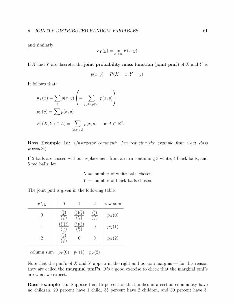
6 JOINTLY DISTRIBUTED RANDOM VARIABLES 61
and similarlyFY (y) = lim
x→∞F (x, y).
If X and Y are discrete, the joint probability mass function (joint pmf) of X and Y is
p(x, y) = P (X = x, Y = y).
It follows that:
pX(x) =∑y
p(x, y)
=∑
y:p(x,y)>0
p(x, y)
pY (y) =
∑x
p(x, y)
P ((X, Y ) ∈ A) =∑
(x,y)∈A
p(x, y) for A ⊂ R2.
Ross Example 1a: (Instructor comment: I’m reducing the example from what Rosspresents.)
If 2 balls are chosen without replacement from an urn containing 3 white, 4 black balls, and5 red balls, let
X = number of white balls chosen
Y = number of black balls chosen.
The joint pmf is given in the following table:
x \ y 0 1 2 row sum
0(52)
(122 )
(41)(
51)
(122 )
(42)
(122 )
pX(0)
1(31)(
51)
(122 )
(31)(
41)
(122 )
0 pX(1)
2(32)
(122 )
0 0 pX(2)
column sum pY (0) pY (1) pY (2)
Note that the pmf’s of X and Y appear in the right and bottom margins — for this reasonthey are called the marginal pmf’s. It’s a good exercise to check that the marginal pmf’sare what we expect.
Ross Example 1b: Suppose that 15 percent of the families in a certain community haveno children, 20 percent have 1 child, 35 percent have 2 children, and 30 percent have 3.
6 JOINTLY DISTRIBUTED RANDOM VARIABLES 62
Suppose further that in each family each child is equally likely (independently) to be aboy or a girl. If a family is chosen at random from this community, then the number Bof boys and the number G of girls in this family will have a joint distribution with values{(i, j) : i, j = 0, . . . , 3}. We have, for example:
P (B = 1, G = 2) = P (B = 1, B +G = 3)
= P (B = 1 | B +G = 3)P (B +G = 3)
=
(3
1
)(1
2
)1(1
2
)2
(.3),
because, given B +G = 3 children, B is binomial(3, 1/2).
X and Y are called jointly continuous if there is a function f = fX,Y : R2 → [0,∞), calledthe joint pdf of X and Y , such that
P ((X, Y ) ∈ C) =
∫∫C
f(x, y) dx dy for nice subsets C ⊂ R2 .
It follows that the joint cdf is
FX,Y (x, y) = P (X ≤ y, Y ≤ x} =
∫ y
−∞
∫ x
−∞f(s, t) ds dt, (x, y) ∈ R2,
and furthermore:
X and Y are continuous;
fX(x) =
∫ ∞−∞
f(x, y) dy and fY (y) =
∫ ∞−∞
f(x, y) dx (marginal pdf’s) ;
f(x, y) =∂2
∂x∂yF (x, y) on any open disk where f is continuous.
Ross Example 1c: The joint pdf of X, Y is
f(x, y) = 2e−xe−2y, x, y > 0.
Compute(a) P (X > 1, Y < 1);
(b) P (X < Y );
(c) P (X < a) for a > 0.
Answer:
6 JOINTLY DISTRIBUTED RANDOM VARIABLES 63
(a)
P (X > 1, Y < 1) =
∫ 1
−∞
∫ ∞1
f(x, y) dx dy
=
∫ 1
0
∫ ∞1
2e−xe−2y dx dy
=
∫ ∞1
e−x dx
∫ 1
0
2e−2y dy
= e−1(1− e−2).
(b)
P (X < Y ) =
∫ ∞0
∫ ∞x
2e−xe−2y dy dx
=
∫ ∞0
e−xe−2x dx
=
∫ ∞0
e−3x dx
=1
3.
(c)
P (X < a) =
∫ ∞−∞
∫ a
−∞f(x, y) dx dy
=
∫ ∞0
∫ a
0
2e−xe−2y dx dy
=
∫ a
0
e−x dx
∫ ∞0
2e−2y dy
= (1− e−a)(1)
= 1− e−a.
Ross Example 1d: Let (X, Y ) be a point randomly chosen in the circle centered at theorigin with radius R. The joint pdf of X, Y is
f(x, y) = c, x2 + y2 ≤ R2,
for some constant c. Find:(a) c;
(b) the marginal density functions of X and Y ;
(c) the probability that the distance D from the point to the origin is no more than a;
6 JOINTLY DISTRIBUTED RANDOM VARIABLES 64
(d) E(D).
Answer:(a) Since f integrates to 1, c must be 1 / area:
c =1
2πR2.
(b) Since (X, Y ) is in the circle, we have −R ≤ X ≤ R, and for x in this interval
fX(x) =
∫ ∞−∞
f(x, y) dy
=
∫ √R2−x2
−√R2−x2
1
2πR2dy
=
√R2 − x2πR2
.
By symmetry,
fY (y) =
√R2 − y2πR2
, −R ≤ y ≤ R.
(c)
P (D ≤ a) = P (X2 + Y 2 ≤ a2)
=
∫∫x2+y2≤a2
1
2πR2dx dy
=2πa2
2πR2=a2
R2.
(d) We have
fD(a) = F ′D(a) =d
da
a2
R2=
2a
R2, 0 ≤ a ≤ R.
Thus
E(D) =
∫ ∞−∞
afD(a) da
=
∫ R
0
2a2
R2da
=2
R2· R
3
3=
2R
3.
Ross Example 1e: The joint pdf of X, Y is
f(x, y) = e−(x+y), x, y > 0.

6 JOINTLY DISTRIBUTED RANDOM VARIABLES 65
Find the pdf of X/Y .
Answer: Since X, Y > 0, so is X/Y , and for t > 0
FX/Y (t) = P (X/Y ≤ t)
= P (X ≤ tY ) (since Y > 0)
=
∫ ∞0
∫ ∞x/t
e−(x+y) dy dx
=
∫ ∞0
e−xe−x/t dx
=
∫ ∞0
e−(1+1/t)x dx
=1
1 + 1/t=
t
t+ 1.
Thus
fX/Y (t) =d
dt
t
t+ 1=
1
(t+ 1)2, t > 0.
Joint probability distributions for n random variables X1, . . . , Xn are defined analogously:the joint cdf is
F (x1, . . . , xn) = P (X1 ≤ x1, . . . , Xn ≤ xn).
When all Xi’s are discrete the joint pmf is
p(x1, . . . , xn) = P (X1 = x1, . . . , Xn = xn),
with marginal pmf’s
pXi(xi) =
∑xj ,j 6=i
p(x1, . . . , xi, . . . , xn).
X1, . . . , Xn are jointly continuous if there is a function f : Rn → [0,∞), the joint pdf,such that
P ((X1, . . . , Xn) ∈ A) =
∫· · ·∫A
f(x1, . . . , xn) dx1, . . . , dxn,
and then
P (X1 ≤ x1, . . . , Xn ≤ xn) =
∫ xn
−∞· · ·∫ x1
−∞f(t1, . . . , tn) dt1 · · · dtn.
I’m skipping Ross Example 1f.
Independent rv’s
Random variables X, Y are independent if
P (X ∈ A, Y ∈ B) = P (X ∈ A)P (Y ∈ B) for all nice subsets A,B ⊂ R,
6 JOINTLY DISTRIBUTED RANDOM VARIABLES 66
equivalently, if the events {X ∈ A} and {Y ∈ B} are independent; dependent means notindependent.
X and Y are independent if and only if
F (x, y) = FX(x)FY (y), (x, y) ∈ R2.
When X and Y are discrete this can be equivalently expressed in terms of the pmf’s:
p(x, y) = pX(x)pY (y) for all x, y,
and when X, Y are jointly continuous it can be expressed in terms of the pdf’s:
f(x, y) = fX(x)fY (y) for all x, y;
in fact, jointly continuous X, Y are independent if and only if
f(x, y) = g(x)h(y) for some g, h : R→ R.
Ross Example 2a: Consider n+m independent Bernoulli(p) trials. Let X = # successesin 1st n trials and Y = # successes in final m trials.(a) X and Y are independent, since
P (X = x, Y = y) =
(n
x
)px(1− p)n−x
(m
y
)py(1− p)m−y = P (X = x)P (Y = y).
(b) Let Z = # successes in the entire n+m trials. Then X and Z are dependent; one wayto verify this is to observe that
P (Z = 0 | X = 1) = 0,
whileP (Z = 0) = (1− p)n+m.
(We’re assuming n,m > 0, 0 < p < 1.)
Ross Example 2b: Suppose that the number of people who enter a post office on a givenday is a Poisson random variable with parameter λ. Show that if each person who enters thepost office is a male with probability p and a female with probability 1− p, then the numberof males and females entering the post office are independent Poisson random variables withrespective parameters λp and λ(1− p).
6 JOINTLY DISTRIBUTED RANDOM VARIABLES 67
Answer: (Instructor comment: Ross has a more efficient solution.) Let M = # males, T =# people. Then
P (M = x) =∞∑t=x
P (M = x, T = t)
=∞∑t=x
P (M = x | T = t)P (T = t)
=∞∑t=x
(t
x
)px(1− p)t−xe−λλ
t
t!
(because, given T = t, M is binomial(t, p))
=pxe−λλx
x!
∞∑t=x
1
(t− x)!(1− p)t−xλt−x
=(λp)xe−λ
x!eλ(1−p)
= e−λp(λp)x
x!.
Thus M is Poisson(λp). Symmetrically, F = # females is Poisson(λ(1− p)).
We still have to show M and F are independent:
P (M = x, F = y) = P (M = x, T = x+ y)
= P (M = x | T = x+ y)P (T = x+ y)
=
(x+ y
x
)px(1− p)ye−λ λx+y
(x+ y)!
=px(1− p)ye−λpe−λ(1−p)λxλy
x!y!
= e−λp(λp)x
x!e−λ(1−p)
(λ(1− p))y
y!
= P (M = x)P (F = y).
Ross Example 2c: A man and a woman decide to meet at a certain location. If each ofthem independently arrives at a time uniformly distributed between 12 noon and 1 PM, findthe probability that the first to arrive has to wait longer than 10 minutes.
Answer: Let X = # hours after 12 that the man arrives, and similarly for Y and the woman.Then X, Y are independent and uniform on (0, 1). The common pdf of X, Y is f(x) = 1,0 < x < 1. By independence,
fX,Y (x, y) = fX(x)fY (y) = 1, 0 < x, y < 1.

6 JOINTLY DISTRIBUTED RANDOM VARIABLES 68
The desired probability is
P (|X − Y | > 1/6) = P (X − Y > 1/6) + P (Y −X > 1/6)
= 2P (Y > X + 1/6) (by symmetry)
= 2
∫ ∞−∞
∫ ∞x+1/6
fX,Y (x, y) dy dx
= 2
∫ 5/6
0
∫ 1
x+1/6
fX,Y (x, y) dy dx
= 2
∫ 5/6
0
∫ 1
x+1/6
dy dx
= 2
∫ 5/6
0
(1− x− 1/6) dx
= 2
∫ 5/6
0
(5/6− x) dx
= 2
∫ 5/6
0
t dt
=
(5
6
)2
.
(Instructor comment: We could have saved a lot of work by just multiplying 2 by the area ofone of the triangles.)
I’m skipping Ross Examples 2d–2e.
Ross Example 2f:(a) If the joint density function of X and Y is
f(x, y) = 6e−2xe−3y, x, y > 0,
are X, Y independent?
(b) What iff(x, y) = 24xy, 0 < x, y < 1, 0 < x+ y < 1?
Answer:(a) Yes, because if g(x) = 2e−2x, x > 0 and h(y) = e−3y, y > 0, then f(x, y) = g(x)h(y).
(b) No, because the restriction 0 < x+y < 1 makes it impossible to write f(x, y) = g(x)h(y).
Independence is defined similarly for n random variables X1, . . . , Xn:
P (X1 ∈ A1, . . . , Xn ∈ An) = P (X1 ∈ A1) · · ·P (Xn ∈ An),
equivalentlyF (x1, . . . , xn) = FX1(x1) · · ·FXn(xn).
6 JOINTLY DISTRIBUTED RANDOM VARIABLES 69
An infinite sequence X1, X2, . . . of random variables is independent if every finite subsetis independent. In all cases dependent means not independent.
I’m skipping Ross Example 2g.
Ross Example 2h: If X, Y, Z are independent and uniformly distributed on (0, 1), findP (X ≥ Y Z).
Answer: By independence we have
fX,Y,Z(x, y, z) = fX(x)fY (y)fZ(z) = 1, 0 < x, y, z < 1.
Thus
P (X ≥ Y Z) =
∫∫∫x≥yz
fX,Y,Z(x, y, z) dx dy dz
=
∫ 1
0
∫ 1
0
∫ 1
yz
dx dy dz
=
∫ 1
0
∫ 1
0
(1− yz) dy dz
=
∫ 1
0
(1− z
2
)dz
= 1− 1
4=
3
4.
I’m skipping the rest of Section 6.2, and Section 6.3.
Conditional distributions
If X and Y are discrete rv’s, the conditional pmf of X given Y = y is
pX|Y (x|y) =pX,Y (x, y)
pY (y).
If X and Y are independent then the conditional pmf is equal to the unconditional one.
Ross Example 4a: Suppose that the joint pmf of X and Y is given by
p(0, 0) = .4, p(0, 1) = .2, p(1, 0) = .1, p(1, 1) = .3.
Calculate the conditional pmf of X given that Y = 1.
Answer: First,
pY (1) = p(0, 1) + p(1, 1) = .2 + .3 = .5.
6 JOINTLY DISTRIBUTED RANDOM VARIABLES 70
Thus
pX|Y (0, 1) =p(0, 1)
pY (1)=.2
.5= .4,
pX|Y (1, 1) =p(1, 1)
pY (1)=.3
.5= .6.
I’m skipping Ross Examples 4b–4d.
If X and Y are jointly continuous rv’s, the conditional pdf of X given Y = y is
fX|Y (x|y) =f(x, y)
fY (y),
and the conditional cdf of X given Y = y is
FX|Y (x|y) =
∫ x
−∞fX|Y (t|y) dt.
More generally,
P (X ∈ A | Y = y) =
∫A
fX|Y (x|y) dx.
If X and Y are independent then the conditional pdf is equal to the unconditional one.
Ross Example 5a: The joint density of X, Y is given by
f(x, y) =12
5x(2− x− y), 0 < x, y < 1.
Compute the conditional density of X given that Y = y for 0 < y < 1.
Answer: First,
fY (y) =
∫ ∞−∞
f(x, y) dx =
∫ 1
0
12
5x(2− x− y) dx =
12
5
(2
3− y
2
),
so
fX|Y (x, y) =f(x, y)
fY (y)=
(12/5)x(2− x− y)
(12/5)(2/3− y/2)=
6x(2− x− y)
4− 3y.
Ross Example 5b: If the joint pdf of X, Y is
f(x, y) =e−x/ye−y
y, x, y > 0,
find P (X > 1 | Y = y).
Answer: First,
fY (y) =
∫ ∞−∞
f(x, y) dx =
∫ ∞0
e−x/ye−y
ydx = e−y.

7 PROPERTIES OF EXPECTATION 71
so
fX|Y (x|y) =f(x, y)
fY (y)=e−x/y
y.
Thus
P (X > 1 | Y = y) =
∫ ∞1
fX|Y (x|y) dx =
∫ ∞1
e−x/y
ydx = e−1/y.
I’m skipping the rest of Ross Chapter 6.
7 Properties of expectation
Let X, Y be jointly distributed random variables. If g : R2 → R, then
E(g(X, Y )) =
{∑x,y g(x, y)p(x, y) (discrete)∫∞−∞
∫∞−∞ g(x, y)f(x, y) dx dy (jointly continuous).
This finally allows for a quick justification that expectation is additive5:
E(X + Y ) =
∫ ∞−∞
∫ ∞−∞
(x+ y)f(x, y) dx dy
=
∫ ∞−∞
∫ ∞−∞
xf(x, y) dx dy +
∫ ∞−∞
∫ ∞−∞
yf(x, y) dx dy
=
∫ ∞−∞
x
∫ ∞−∞
f(x, y) dy dx+
∫ ∞−∞
y
∫ ∞−∞
f(x, y) dx dy
=
∫ ∞−∞
xfX(x) dx+
∫ ∞−∞
yfY (y) dy
= EX + EY.
Ross Example 2a: An accident occurs at a point X that is uniformly distributed on aroad of length L. At the time of the accident, an ambulance is at a location Y that isalso uniformly distributed on the road. Assuming that X and Y are independent, find theexpected distance between the ambulance and the point of the accident.
Answer: By independence,
fX,Y (x, y) = fX(x)fY (y) =
(1
L
)2
, 0 < x, y < L.
5in the continuous case — the discrete case is similar

7 PROPERTIES OF EXPECTATION 72
Thus the expected distance is
E|X − Y | =∫ ∞−∞
∫ ∞−∞|x− y|fX,Y (x, y) dx dy
=
∫ L
0
∫ L
0
|x− y|L2
dx dy
=2
L2
∫ L
0
∫ x
0
(x− y) dy dx (by symmetry)
=2
L2
∫ L
0
(x2 − x2
2
)dy
=2
L2
∫ L
0
x2
2dy
=1
L2
L3
3=L
3.
Ross Example 2c: (Sample mean) Let X1, . . . , Xn be independent and identically dis-tributed random variables having distribution function F and expected value µ. Such asequence of rv’s is called a sample from the distribution F . The quantity
X =1
n
n∑i=1
Xi
is called the sample mean. Find EX.
Answer: By independence, and by linearity of expectation,
EX =1
n
n∑i=1
EXi =1
n
n∑i=1
µ = µ.
I’m skipping Ross Example 2d.
Number of events that occur
Consider events A1, . . . , An in our sample space, and let X = the number of these eventsthat occur. Then
X =n∑i=1
IAi,
where IAiis the indicator rv of Ai, so
EX =n∑i=1
EIAi=
n∑i=1
P (Ai).
7 PROPERTIES OF EXPECTATION 73
Ross Example 2e: (Mean of binomial) (Instructor comment: We gave this derivation inChapter 4.) Let X be binomial(n, p). Since X represents the number of successes in nindependent Bernoulli(p) trials,
X =n∑i=1
Xi,
where Xi is the indicator variable of success on the ith trial. Each Xi is Bernoulli(p), soEXi = p, and hence
EX =n∑i=1
EXi = np.
But now we can view it another way: X is the number of the events {Xi = 1} that occur,each with probability p, so
EX =n∑i=1
p = np.
Ross Example 2f: (Mean of negative binomial) Let X be negative binomial(r, p). Since Xrepresents the number of trials until r successes in independent Bernoulli(p) trials,
X =r∑i=1
Xi,
where Xi is the number of additional trials, after the (i− 1)st success, until the ith success.Each Xi is geometric(p), so EXi = 1/p, and hence
EX =n∑i=1
EXi =n
p.
(Instructor comment: Note that we could not apply the “number of events that occur” methodhere since the Xi’s are not Bernoulli r.v.’s.)
Ross Example 2h: (Expected number of matches) Suppose that N people throw their hatsinto the center of a room. The hats are mixed up, and each person randomly selects one.Find the expected number of people that select their own hat.
Answer: Let X = # that get their own hat. Then
EX =N∑i=1
P (ith person gets own hat) = N · 1
N= 1.
Ross Example 2i: (Coupon-collecting problem) Suppose that there are N different typesof coupons, and each time one obtains a coupon, it is equally likely to be any one of the Ntypes. Find the expected number of coupons needed to get a complete set.

7 PROPERTIES OF EXPECTATION 74
Answer: Let X = # coupons needed to get a complete set. Then
X =N−1∑i=0
Xi,
where Xi is the number of additional coupons needed, after i types have been obtained, toobtain another type. For each i, there are N − i types left to collect, and the probability ofthe next coupon being any one of these is 1/N , so the probability of the next coupon beinga new type is (N − i)/N . Thus Xi is geometric with parameter (N − i)/N , so
EX =N−1∑i=0
EXi =N−1∑i=0
N
N − i= N
N∑i=1
1
i.
Ross Example 2j: Ten hunters are waiting for ducks to fly by. When a flock of ducksflies overhead, the hunters fire at the same time, but each chooses his target at random,independently of the others. If each hunter independently hits his target with probabilityp, compute the expected number of ducks that escape unhurt when a flock of size 10 fliesoverhead.
Answer: Let X = # ducks not hit. Then
EX =10∑i=1
P (ith duck not hit)
= 10P (1st duck not hit) (by symmetry)
= 10(P (1st duck not hit by 1st hunter)
)10(by symmetry and independence).
The events {1st hunter chooses 1st duck as target} and {1st hunter hits target} are inde-pendent, with probabilities 1/10 and p respectively, so
P (1st duck is hit by 1st hunter) =p
10,
and henceP (1st duck is not hit by 1st hunter) = 1− p
10.
Therefore
EX = 10(
1− p
10
)10.
I’m skipping the rest of Ross Section 7.2, and most of Section 7.3, except we already coveredE(number of events that occur).

7 PROPERTIES OF EXPECTATION 75
Variance of sums
Suppose X and Y are independent rv’s. In the continuous case,
E(g(X)h(Y )) =
∫ ∞−∞
∫ ∞−∞
g(x)h(y)fX,Y (x, y) dx dy
=
∫ ∞−∞
∫ ∞−∞
g(x)h(y)fX(x)fY (y) dx dy
=
∫ ∞−∞
g(x)fX(x) dx
∫ ∞−∞
h(y)fY (y) dy
= E(g(X))E(h(Y )).
Similarly (and more easily) in the discrete case. Thus
Var(X + Y ) = E((X + Y )2)− (E(X + Y ))2
= E(X2 + Y 2 + 2XY )− (EX + EY )2
= E(X2) + E(Y 2) + 2E(XY )− (EX)2 − (EY )2 − 2(EX)(EY )
= Var(X) + Var(Y ) + 2(EX)(EY )− 2(EX)(EY )
= Var(X) + Var(Y ).
Similarly (by induction), if X1, . . . , Xn are independent then
Var
(n∑i=1
Xi
)=
n∑i=1
Var(Xi).
Ross Example 4a: Let X1, . . . , Xn be independent and identically distributed rv’s withexpected value µ and variance σ2, and let X =
∑ni=1Xi/n be the sample mean. The sample
variance is
S2 =1
n− 1
n∑i=1
(Xi −X)2.
Find:(a) Var(X);
(b) E(S2).
Answer:(a) By independence,
Var(X) =1
n2
n∑i=1
Var(Xi) =σ2
n.
7 PROPERTIES OF EXPECTATION 76
(b) First note that
(n− 1)S2 =n∑i=1
(Xi − µ+ µ−X
)2=
n∑i=1
(Xi − µ)2 +n∑i=1
(µ−X)2 + 2(µ−X)n∑i=1
(Xi − µ)
=n∑i=1
(Xi − µ)2 + n(X − µ)2 − 2(X − µ)n(X − µ)
=n∑i=1
(Xi − µ)2 − n(X − µ)2.
Thus
(n− 1)E(S2) =n∑i=1
E((Xi − µ)2
)− nE
((X − µ)2
)= nσ2 − nVar(X)
= (n− 1)σ2,
and henceE(S2) = σ2.
Ross Example 4b: (Variance of a binomial) Let X be binomial(n, p). We’ve seen thatX =
∑ni=1Xi, where X1, . . . , Xn are independent Bernoulli(p) rv’s. Thus
Var(X) = nVar(Xi) = np(1− p).
Similarly, if X is negative binomial(r, p), recall that X =∑r
i=1, where Xi = number ofadditional trials, after (i− 1)st success, until ith success. Since the Xi’s are combinations ofnonoverlapping sets of independent rv’s, they are independent geometric(p) rv’s, so
Var(X) = rVar(Xi) =r(1− p)p2
.
I’m skipping the rest of Ross Section 7.4.
Conditional expectation
The conditional expectation of X given Y = y is
E(X | Y = y) =
{∑x xpX|Y (x|y) (discrete)∫∞−∞ xfX|Y (x|y) dx (jointly continuous.
7 PROPERTIES OF EXPECTATION 77
Properties:
E(g(X) | Y = y) =
{∑x g(x)pX|Y (x|y) (discrete)∫∞−∞ g(x)fX|Y (x|y) dx (jointly continuous)
E(aX + bZ | Y = y) = aE(X | Y = y) + bE(Z | Y = y)
(linearity of conditional expectation)
I’m skipping Ross Example 5a.
Ross Example 5b: Suppose the joint density of X, Y is
f(x, y) =e−x/ye−y
y, x, y > 0.
Compute E(X | Y = y).
Answer: First,
fY (y) =
∫ ∞−∞
f(x, y) dx
=
∫ ∞0
e−x/ye−y
ydx
= e−y,
so
fX|Y (x|y) =f(x, y)
fY (y)=e−x/y
y.
Thus the conditional distribution of X given Y = y is exponential(1/y), so
E(X | Y = y) = y.
We write E(X|Y ) for rv g(Y ) given by
g(y) = E(X | Y = y).
The expectation of this rv isE(E(X|Y )) = EX.
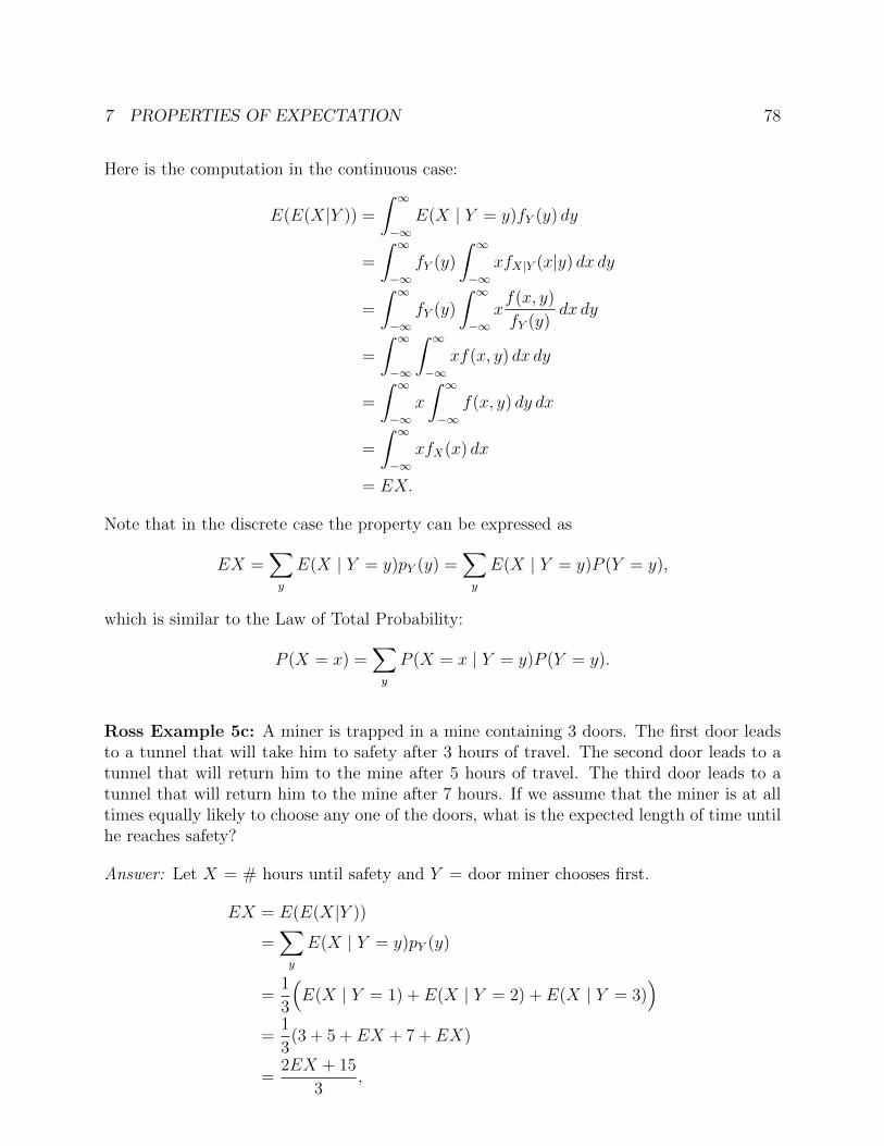
7 PROPERTIES OF EXPECTATION 78
Here is the computation in the continuous case:
E(E(X|Y )) =
∫ ∞−∞
E(X | Y = y)fY (y) dy
=
∫ ∞−∞
fY (y)
∫ ∞−∞
xfX|Y (x|y) dx dy
=
∫ ∞−∞
fY (y)
∫ ∞−∞
xf(x, y)
fY (y)dx dy
=
∫ ∞−∞
∫ ∞−∞
xf(x, y) dx dy
=
∫ ∞−∞
x
∫ ∞−∞
f(x, y) dy dx
=
∫ ∞−∞
xfX(x) dx
= EX.
Note that in the discrete case the property can be expressed as
EX =∑y
E(X | Y = y)pY (y) =∑y
E(X | Y = y)P (Y = y),
which is similar to the Law of Total Probability:
P (X = x) =∑y
P (X = x | Y = y)P (Y = y).
Ross Example 5c: A miner is trapped in a mine containing 3 doors. The first door leadsto a tunnel that will take him to safety after 3 hours of travel. The second door leads to atunnel that will return him to the mine after 5 hours of travel. The third door leads to atunnel that will return him to the mine after 7 hours. If we assume that the miner is at alltimes equally likely to choose any one of the doors, what is the expected length of time untilhe reaches safety?
Answer: Let X = # hours until safety and Y = door miner chooses first.
EX = E(E(X|Y ))
=∑y
E(X | Y = y)pY (y)
=1
3
(E(X | Y = 1) + E(X | Y = 2) + E(X | Y = 3)
)=
1
3(3 + 5 + EX + 7 + EX)
=2EX + 15
3,
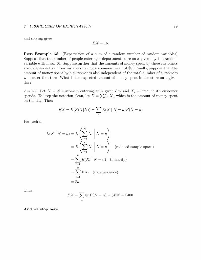
7 PROPERTIES OF EXPECTATION 79
and solving givesEX = 15.
Ross Example 5d: (Expectation of a sum of a random number of random variables)Suppose that the number of people entering a department store on a given day is a randomvariable with mean 50. Suppose further that the amounts of money spent by these customersare independent random variables having a common mean of $8. Finally, suppose that theamount of money spent by a customer is also independent of the total number of customerswho enter the store. What is the expected amount of money spent in the store on a givenday?
Answer: Let N = # customers entering on a given day and Xi = amount ith customerspends. To keep the notation clean, let X =
∑Ni=1Xi, which is the amount of money spent
on the day. Then
EX = E(E(X|N)) =∑n
E(X | N = n)P (N = n)
For each n,
E(X | N = n) = E
(N∑i=1
Xi
∣∣∣∣ N = n
)
= E
(n∑i=1
Xi
∣∣∣∣ N = n
)(reduced sample space)
=n∑i=1
E(Xi | N = n) (linearity)
=n∑i=1
EXi (independence)
= 8n
ThusEX =
∑n
8nP (N = n) = 8EN = $400.
And we stop here.