notes on probability - always busy counting, doubting ... · notes on probability peter j. cameron....
TRANSCRIPT

Notes on Probability
Peter J. Cameron

ii
Preface
Here are the course lecture notes for the course MAS108, Probability I, at QueenMary, University of London, taken by most Mathematics students and some othersin the first semester.
The description of the course is as follows:
This course introduces the basic notions of probability theory and de-velops them to the stage where one can begin to use probabilisticideas in statistical inference and modelling, and the study of stochasticprocesses. Probability axioms. Conditional probability and indepen-dence. Discrete random variables and their distributions. Continuousdistributions. Joint distributions. Independence. Expectations. Mean,variance, covariance, correlation. Limiting distributions.
The syllabus is as follows:
1. Basic notions of probability. Sample spaces, events, relative frequency,probability axioms.
2. Finite sample spaces. Methods of enumeration. Combinatorial probability.
3. Conditional probability. Theorem of total probability. Bayes theorem.
4. Independence of two events. Mutual independence of n events. Samplingwith and without replacement.
5. Random variables. Univariate distributions - discrete, continuous, mixed.Standard distributions - hypergeometric, binomial, geometric, Poisson, uni-form, normal, exponential. Probability mass function, density function, dis-tribution function. Probabilities of events in terms of random variables.
6. Transformations of a single random variable. Mean, variance, median,quantiles.
7. Joint distribution of two random variables. Marginal and conditional distri-butions. Independence.
iii
iv
8. Covariance, correlation. Means and variances of linear functions of randomvariables.
9. Limiting distributions in the Binomial case.
These course notes explain the naterial in the syllabus. They have been “field-tested” on the class of 2000. Many of the examples are taken from the coursehomework sheets or past exam papers.
Set books The notes cover only material in the Probability I course. The text-books listed below will be useful for other courses on probability and statistics.You need at most one of the three textbooks listed below, but you will need thestatistical tables.
• Probability and Statistics for Engineering and the Sciences by Jay L. De-vore (fifth edition), published by Wadsworth.
Chapters 2–5 of this book are very close to the material in the notes, both inorder and notation. However, the lectures go into more detail at several points,especially proofs. If you find the course difficult then you are advised to buythis book, read the corresponding sections straight after the lectures, and do extraexercises from it.
Other books which you can use instead are:
• Probability and Statistics in Engineering and Management Science by W. W.Hines and D. C. Montgomery, published by Wiley, Chapters 2–8.
• Mathematical Statistics and Data Analysis by John A. Rice, published byWadsworth, Chapters 1–4.
You should also buy a copy of
• New Cambridge Statistical Tables by D. V. Lindley and W. F. Scott, pub-lished by Cambridge University Press.
You need to become familiar with the tables in this book, which will be providedfor you in examinations. All of these books will also be useful to you in thecourses Statistics I and Statistical Inference.
The next book is not compulsory but introduces the ideas in a friendly way:
• Taking Chances: Winning with Probability, by John Haigh, published byOxford University Press.
v
Web resources Course material for the MAS108 course is kept on the Web atthe address
http://www.maths.qmw.ac.uk/˜pjc/MAS108/
This includes a preliminary version of these notes, together with courseworksheets, test and past exam papers, and some solutions.
Other web pages of interest include
http://www.dartmouth.edu/˜chance/teaching aids/books articles/probability book/pdf.html
A textbook Introduction to Probability, by Charles M. Grinstead and J. LaurieSnell, available free, with many exercises.
http://www.math.uah.edu/stat/
The Virtual Laboratories in Probability and Statistics, a set of web-based resourcesfor students and teachers of probability and statistics, where you can run simula-tions etc.
http://www.newton.cam.ac.uk/wmy2kposters/july/
The Birthday Paradox (poster in the London Underground, July 2000).
http://www.combinatorics.org/Surveys/ds5/VennEJC.html
An article on Venn diagrams by Frank Ruskey, with history and many nice pic-tures.
Web pages for other Queen Mary maths courses can be found from the on-lineversion of the Maths Undergraduate Handbook.
Peter J. CameronDecember 2000

vi
Contents
1 Basic ideas 11.1 Sample space, events . . . . . . . . . . . . . . . . . . . . . . . . 11.2 What is probability? . . . . . . . . . . . . . . . . . . . . . . . . . 31.3 Kolmogorov’s Axioms . . . . . . . . . . . . . . . . . . . . . . . 31.4 Proving things from the axioms . . . . . . . . . . . . . . . . . . . 41.5 Inclusion-Exclusion Principle . . . . . . . . . . . . . . . . . . . . 61.6 Other results about sets . . . . . . . . . . . . . . . . . . . . . . . 71.7 Sampling . . . . . . . . . . . . . . . . . . . . . . . . . . . . . . 81.8 Stopping rules . . . . . . . . . . . . . . . . . . . . . . . . . . . . 121.9 Questionnaire results . . . . . . . . . . . . . . . . . . . . . . . . 131.10 Independence . . . . . . . . . . . . . . . . . . . . . . . . . . . . 141.11 Mutual independence . . . . . . . . . . . . . . . . . . . . . . . . 161.12 Properties of independence . . . . . . . . . . . . . . . . . . . . . 171.13 Worked examples . . . . . . . . . . . . . . . . . . . . . . . . . . 20
2 Conditional probability 232.1 What is conditional probability? . . . . . . . . . . . . . . . . . . 232.2 Genetics . . . . . . . . . . . . . . . . . . . . . . . . . . . . . . . 252.3 The Theorem of Total Probability . . . . . . . . . . . . . . . . . 262.4 Sampling revisited . . . . . . . . . . . . . . . . . . . . . . . . . 282.5 Bayes’ Theorem . . . . . . . . . . . . . . . . . . . . . . . . . . . 292.6 Iterated conditional probability . . . . . . . . . . . . . . . . . . . 312.7 Worked examples . . . . . . . . . . . . . . . . . . . . . . . . . . 34
3 Random variables 393.1 What are random variables? . . . . . . . . . . . . . . . . . . . . 393.2 Probability mass function . . . . . . . . . . . . . . . . . . . . . . 403.3 Expected value and variance . . . . . . . . . . . . . . . . . . . . 413.4 Joint p.m.f. of two random variables . . . . . . . . . . . . . . . . 433.5 Some discrete random variables . . . . . . . . . . . . . . . . . . 473.6 Continuous random variables . . . . . . . . . . . . . . . . . . . . 55
vii
viii CONTENTS
3.7 Median, quartiles, percentiles . . . . . . . . . . . . . . . . . . . . 573.8 Some continuous random variables . . . . . . . . . . . . . . . . . 583.9 On using tables . . . . . . . . . . . . . . . . . . . . . . . . . . . 613.10 Worked examples . . . . . . . . . . . . . . . . . . . . . . . . . . 63
4 More on joint distribution 674.1 Covariance and correlation . . . . . . . . . . . . . . . . . . . . . 674.2 Conditional random variables . . . . . . . . . . . . . . . . . . . . 704.3 Joint distribution of continuous r.v.s . . . . . . . . . . . . . . . . 734.4 Transformation of random variables . . . . . . . . . . . . . . . . 744.5 Worked examples . . . . . . . . . . . . . . . . . . . . . . . . . . 77
A Mathematical notation 79
B Probability and random variables 83
Chapter 1
Basic ideas
In this chapter, we don’t really answer the question ‘What is probability?’ No-body has a really good answer to this question. We take a mathematical approach,writing down some basic axioms which probability must satisfy, and making de-ductions from these. We also look at different kinds of sampling, and examinewhat it means for events to be independent.
1.1 Sample space, eventsThe general setting is: We perform an experiment which can have a number ofdifferent outcomes. The sample space is the set of all possible outcomes of theexperiment. We usually call it S .
It is important to be able to list the outcomes clearly. For example, if I plantten bean seeds and count the number that germinate, the sample space is
S = 0,1,2,3,4,5,6,7,8,9,10.
If I toss a coin three times and record the result, the sample space is
S = HHH,HHT,HT H,HT T,T HH,T HT,T T H,T T T,
where (for example) HT H means ‘heads on the first toss, then tails, then headsagain’.
Sometimes we can assume that all the outcomes are equally likely. (Don’tassume this unless either you are told to, or there is some physical reason forassuming it. In the beans example, it is most unlikely. In the coins example,the assumption will hold if the coin is ‘fair’: this means that there is no physicalreason for it to favour one side over the other.) If all outcomes are equally likely,then each has probability 1/|S |. (Remember that |S | is the number of elements inthe set S ).
1
2 CHAPTER 1. BASIC IDEAS
On this point, Albert Einstein wrote, in his 1905 paper On a heuristic pointof view concerning the production and transformation of light (for which he wasawarded the Nobel Prize),
In calculating entropy by molecular-theoretic methods, the word “prob-ability” is often used in a sense differing from the way the word isdefined in probability theory. In particular, “cases of equal probabil-ity” are often hypothetically stipulated when the theoretical methodsemployed are definite enough to permit a deduction rather than a stip-ulation.
In other words: Don’t just assume that all outcomes are equally likely, especiallywhen you are given enough information to calculate their probabilities!
An event is a subset of S . We can specify an event by listing all the outcomesthat make it up. In the above example, let A be the event ‘more heads than tails’and B the event ‘heads on last throw’. Then
A = HHH,HHT,HT H,T HH,B = HHH,HT H,T HH,T T H.
The probability of an event is calculated by adding up the probabilities of allthe outcomes comprising that event. So, if all outcomes are equally likely, wehave
P(A) =|A||S |
.
In our example, both A and B have probability 4/8 = 1/2.An event is simple if it consists of just a single outcome, and is compound
otherwise. In the example, A and B are compound events, while the event ‘headson every throw’ is simple (as a set, it is HHH). If A = a is a simple event,then the probability of A is just the probability of the outcome a, and we usuallywrite P(a), which is simpler to write than P(a). (Note that a is an outcome,while a is an event, indeed a simple event.)
We can build new events from old ones:
• A∪B (read ‘A union B’) consists of all the outcomes in A or in B (or both!)
• A∩B (read ‘A intersection B’) consists of all the outcomes in both A and B;
• A\B (read ‘A minus B’) consists of all the outcomes in A but not in B;
• A′ (read ‘A complement’) consists of all outcomes not in A (that is, S \A);
• /0 (read ‘empty set’) for the event which doesn’t contain any outcomes.

1.2. WHAT IS PROBABILITY? 3
Note the backward-sloping slash; this is not the same as either a vertical slash | ora forward slash /.
In the example, A′ is the event ‘more tails than heads’, and A∩B is the eventHHH,T HH,HT H. Note that P(A∩B) = 3/8; this is not equal to P(A) ·P(B),despite what you read in some books!
1.2 What is probability?
There is really no answer to this question.Some people think of it as ‘limiting frequency’. That is, to say that the proba-
bility of getting heads when a coin is tossed means that, if the coin is tossed manytimes, it is likely to come down heads about half the time. But if you toss a coin1000 times, you are not likely to get exactly 500 heads. You wouldn’t be surprisedto get only 495. But what about 450, or 100?
Some people would say that you can work out probability by physical argu-ments, like the one we used for a fair coin. But this argument doesn’t work in allcases, and it doesn’t explain what probability means.
Some people say it is subjective. You say that the probability of heads in acoin toss is 1/2 because you have no reason for thinking either heads or tails morelikely; you might change your view if you knew that the owner of the coin was amagician or a con man. But we can’t build a theory on something subjective.
We regard probability as a mathematical construction satisfying some axioms(devised by the Russian mathematician A. N. Kolmogorov). We develop ways ofdoing calculations with probability, so that (for example) we can calculate howunlikely it is to get 480 or fewer heads in 1000 tosses of a fair coin. The answeragrees well with experiment.
1.3 Kolmogorov’s Axioms
Remember that an event is a subset of the sample space S . A number of events,say A1,A2, . . ., are called mutually disjoint or pairwise disjoint if Ai∩A j = /0 forany two of the events Ai and A j; that is, no two of the events overlap.
According to Kolmogorov’s axioms, each event A has a probability P(A),which is a number. These numbers satisfy three axioms:
Axiom 1: For any event A, we have P(A)≥ 0.
Axiom 2: P(S) = 1.
4 CHAPTER 1. BASIC IDEAS
Axiom 3: If the events A1,A2, . . . are pairwise disjoint, then
P(A1∪A2∪·· ·) = P(A1)+P(A2)+ · · ·
Note that in Axiom 3, we have the union of events and the sum of numbers.Don’t mix these up; never write P(A1)∪P(A2), for example. Sometimes we sep-arate Axiom 3 into two parts: Axiom 3a if there are only finitely many eventsA1,A2, . . . ,An, so that we have
P(A1∪·· ·∪An) =n
∑i=1
P(Ai),
and Axiom 3b for infinitely many. We will only use Axiom 3a, but 3b is importantlater on.
Notice that we writen
∑i=1
P(Ai)
forP(A1)+P(A2)+ · · ·+P(An).
1.4 Proving things from the axiomsYou can prove simple properties of probability from the axioms. That means,every step must be justified by appealing to an axiom. These properties seemobvious, just as obvious as the axioms; but the point of this game is that we assumeonly the axioms, and build everything else from that.
Here are some examples of things proved from the axioms. There is really nodifference between a theorem, a proposition, and a corollary; they all have to beproved. Usually, a theorem is a big, important statement; a proposition a rathersmaller statement; and a corollary is something that follows quite easily from atheorem or proposition that came before.
Proposition 1.1 If the event A contains only a finite number of outcomes, sayA = a1,a2, . . . ,an, then
P(A) = P(a1)+P(a2)+ · · ·+P(an).
To prove the proposition, we define a new event Ai containing only the out-come ai, that is, Ai = ai, for i = 1, . . . ,n. Then A1, . . . ,An are mutually disjoint
1.4. PROVING THINGS FROM THE AXIOMS 5
(each contains only one element which is in none of the others), and A1 ∪A2 ∪·· ·∪An = A; so by Axiom 3a, we have
P(A) = P(a1)+P(a2)+ · · ·+P(an).
Corollary 1.2 If the sample space S is finite, say S = a1, . . . ,an, then
P(a1)+P(a2)+ · · ·+P(an) = 1.
For P(a1)+P(a2)+ · · ·+ P(an) = P(S) by Proposition 1.1, and P(S) = 1 byAxiom 2. Notice that once we have proved something, we can use it on the samebasis as an axiom to prove further facts.
Now we see that, if all the n outcomes are equally likely, and their probabil-ities sum to 1, then each has probability 1/n, that is, 1/|S |. Now going back toProposition 1.1, we see that, if all outcomes are equally likely, then
P(A) =|A||S |
for any event A, justifying the principle we used earlier.
Proposition 1.3 P(A′) = 1−P(A) for any event A.
Let A1 = A and A2 = A′ (the complement of A). Then A1∩A2 = /0 (that is, theevents A1 and A2 are disjoint), and A1∪A2 = S . So
P(A1)+P(A2) = P(A1∪A2) (Axiom 3)= P(S)= 1 (Axiom 2).
So P(A) = P(A1) = 1−P(A2).
Corollary 1.4 P(A)≤ 1 for any event A.
For 1−P(A) = P(A′) by Proposition 1.3, and P(A′) ≥ 0 by Axiom 1; so 1−P(A)≥ 0, from which we get P(A)≤ 1.
Remember that if you ever calculate a probability to be less than 0 or morethan 1, you have made a mistake!
Corollary 1.5 P( /0) = 0.
For /0 = S ′, so P( /0) = 1−P(S) by Proposition 1.3; and P(S) = 1 by Axiom 2,so P( /0) = 0.
6 CHAPTER 1. BASIC IDEAS
Here is another result. The notation A⊆ B means that A is contained in B, thatis, every outcome in A also belongs to B.
Proposition 1.6 If A ⊆ B, then P(A)≤ P(B).
This time, take A1 = A, A2 = B \A. Again we have A1 ∩A2 = /0 (since theelements of B\A are, by definition, not in A), and A1∪A2 = B. So by Axiom 3,
P(A1)+P(A2) = P(A1∪A2) = P(B).
In other words, P(A)+P(B\A) = P(B). Now P(B\A)≥ 0 by Axiom 1; so
P(A)≤ P(B),
as we had to show.
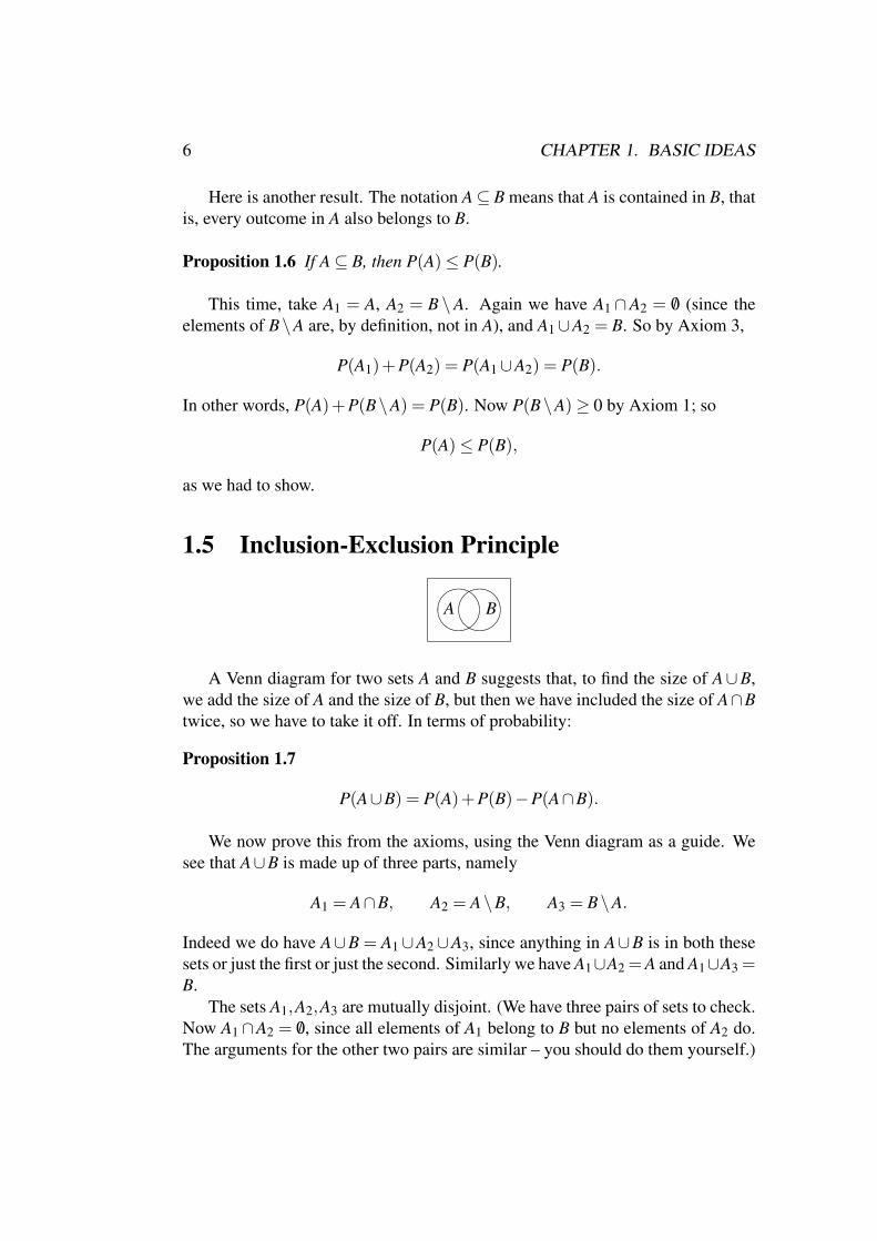
1.5 Inclusion-Exclusion Principle
A B
A Venn diagram for two sets A and B suggests that, to find the size of A∪B,we add the size of A and the size of B, but then we have included the size of A∩Btwice, so we have to take it off. In terms of probability:
Proposition 1.7
P(A∪B) = P(A)+P(B)−P(A∩B).
We now prove this from the axioms, using the Venn diagram as a guide. Wesee that A∪B is made up of three parts, namely
A1 = A∩B, A2 = A\B, A3 = B\A.
Indeed we do have A∪B = A1∪A2∪A3, since anything in A∪B is in both thesesets or just the first or just the second. Similarly we have A1∪A2 = A and A1∪A3 =B.
The sets A1,A2,A3 are mutually disjoint. (We have three pairs of sets to check.Now A1∩A2 = /0, since all elements of A1 belong to B but no elements of A2 do.The arguments for the other two pairs are similar – you should do them yourself.)

1.6. OTHER RESULTS ABOUT SETS 7
So, by Axiom 3, we have
P(A) = P(A1)+P(A2),P(B) = P(A1)+P(A3),
P(A∪B) = P(A1)+P(A2)+P(A3).
From this we obtain
P(A)+P(B)−P(A∩B) = (P(A1)+P(A2))+(P(A1)+P(A3))−P(A1)= P(A1)+P(A2)+P(A3)= P(A∪B)
as required.
The Inclusion-Exclusion Principle extends to more than two events, but getsmore complicated. Here it is for three events; try to prove it yourself.
A B
C
To calculate P(A∪B∪C), we first add up P(A), P(B), and P(C). The parts incommon have been counted twice, so we subtract P(A∩B), P(A∩C) and P(B∩C).But then we find that the outcomes lying in all three sets have been taken offcompletely, so must be put back, that is, we add P(A∩B∩C).
Proposition 1.8 For any three events A,B,C, we have
P(A∪B∪C)= P(A)+P(B)+P(C)−P(A∩B)−P(A∩C)−P(B∩C)+P(A∩B∩C).
Can you extend this to any number of events?
1.6 Other results about setsThere are other standard results about sets which are often useful in probabilitytheory. Here are some examples.
Proposition 1.9 Let A,B,C be subsets of S .
Distributive laws: (A∩B)∪C = (A∪C)∩ (B∪C) and(A∪B)∩C = (A∩C)∪ (B∩C).
De Morgan’s Laws: (A∪B)′ = A′∩B′ and (A∩B)′ = A′∪B′.
We will not give formal proofs of these. You should draw Venn diagrams andconvince yourself that they work.
8 CHAPTER 1. BASIC IDEAS
1.7 SamplingI have four pens in my desk drawer; they are red, green, blue, and purple. I draw apen; each pen has the same chance of being selected. In this case, S = R,G,B,P,where R means ‘red pen chosen’ and so on. In this case, if A is the event ‘red orgreen pen chosen’, then
P(A) =|A||S |
=24
=12.
More generally, if I have a set of n objects and choose one, with each oneequally likely to be chosen, then each of the n outcomes has probability 1/n, andan event consisting of m of the outcomes has probability m/n.
What if we choose more than one pen? We have to be more careful to specifythe sample space.
First, we have to say whether we are
• sampling with replacement, or
• sampling without replacement.
Sampling with replacement means that we choose a pen, note its colour, putit back and shake the drawer, then choose a pen again (which may be the samepen as before or a different one), and so on until the required number of pens havebeen chosen. If we choose two pens with replacement, the sample space is
RR, RG, RB, RP,GR, GG, GB, GP,BR, BG, BB, BP,PR, PG, PB, PP
The event ‘at least one red pen’ is RR,RG,RB,RP,GR,BR,PR, and has proba-bility 7/16.
Sampling without replacement means that we choose a pen but do not put itback, so that our final selection cannot include two pens of the same colour. Inthis case, the sample space for choosing two pens is
RG, RB, RP,GR, GB, GP,BR, BG, BP,PR, PG, PB
and the event ‘at least one red pen’ is RG,RB,RP,GR,BR,PR, with probability6/12 = 1/2.
1.7. SAMPLING 9
Now there is another issue, depending on whether we care about the order inwhich the pens are chosen. We will only consider this in the case of samplingwithout replacement. It doesn’t really matter in this case whether we choose thepens one at a time or simply take two pens out of the drawer; and we are notinterested in which pen was chosen first. So in this case the sample space is
R,G,R,B,R,P,G,B,G,P,B,P,
containing six elements. (Each element is written as a set since, in a set, we don’tcare which element is first, only which elements are actually present. So the sam-ple space is a set of sets!) The event ‘at least one red pen’ is R,G,R,B,R,P,with probability 3/6 = 1/2. We should not be surprised that this is the same as inthe previous case.
There are formulae for the sample space size in these three cases. These in-volve the following functions:
n! = n(n−1)(n−2) · · ·1nPk = n(n−1)(n−2) · · ·(n− k +1)nCk = nPk/k!
Note that n! is the product of all the whole numbers from 1 to n; and
nPk =n!
(n− k)!,
so thatnCk =
n!k!(n− k)!
.
Theorem 1.10 The number of selections of k objects from a set of n objects isgiven in the following table.
with replacement without replacementordered sample nk nPk
unordered sample nCk
In fact the number that goes in the empty box is n+k−1Ck, but this is muchharder to prove than the others, and you are very unlikely to need it.
Here are the proofs of the other three cases. First, for sampling with replace-ment and ordered sample, there are n choices for the first object, and n choicesfor the second, and so on; we multiply the choices for different objects. (Think ofthe choices as being described by a branching tree.) The product of k factors eachequal to n is nk.
10 CHAPTER 1. BASIC IDEAS
For sampling without replacement and ordered sample, there are still n choicesfor the first object, but now only n− 1 choices for the second (since we do notreplace the first), and n−2 for the third, and so on; there are n− k +1 choices forthe kth object, since k−1 have previously been removed and n− (k−1) remain.As before, we multiply. This product is the formula for nPk.
For sampling without replacement and unordered sample, think first of choos-ing an ordered sample, which we can do in nPk ways. But each unordered samplecould be obtained by drawing it in k! different orders. So we divide by k!, obtain-ing nPk/k! = nCk choices.
In our example with the pens, the numbers in the three boxes are 42 = 16,4P2 = 12, and 4C2 = 6, in agreement with what we got when we wrote them allout.
Note that, if we use the phrase ‘sampling without replacement, ordered sam-ple’, or any other combination, we are assuming that all outcomes are equallylikely.
Example The names of the seven days of the week are placed in a hat. Threenames are drawn out; these will be the days of the Probability I lectures. What isthe probability that no lecture is scheduled at the weekend?
Here the sampling is without replacement, and we can take it to be eitherordered or unordered; the answers will be the same. For ordered samples, thesize of the sample space is 7P3 = 7 · 6 · 5 = 210. If A is the event ‘no lectures atweekends’, then A occurs precisely when all three days drawn are weekdays; so|A|= 5P3 = 5 ·4 ·3 = 60. Thus, P(A) = 60/210 = 2/7.
If we decided to use unordered samples instead, the answer would be 5C3/7C3,
which is once again 2/7.
Example A six-sided die is rolled twice. What is the probability that the sum ofthe numbers is at least 10?
This time we are sampling with replacement, since the two numbers may bethe same or different. So the number of elements in the sample space is 62 = 36.
To obtain a sum of 10 or more, the possibilities for the two numbers are (4,6),(5,5), (6,4), (5,6), (6,5) or (6,6). So the probability of the event is 6/36 = 1/6.
Example A box contains 20 balls, of which 10 are red and 10 are blue. We drawten balls from the box, and we are interested in the event that exactly 5 of the ballsare red and 5 are blue. Do you think that this is more likely to occur if the drawsare made with or without replacement?
Let S be the sample space, and A the event that five balls are red and five areblue.
1.7. SAMPLING 11
Consider sampling with replacement. Then |S | = 2010. What is |A|? Thenumber of ways in which we can choose first five red balls and then five blue ones(that is, RRRRRBBBBB), is 105 ·105 = 1010. But there are many other ways to getfive red and five blue balls. In fact, the five red balls could appear in any five ofthe ten draws. This means that there are 10C5 = 252 different patterns of five Rsand five Bs. So we have
|A|= 252 ·1010,
and so
P(A) =252 ·1010
2010 = 0.246 . . .
Now consider sampling without replacement. If we regard the sample as beingordered, then |S | = 20P10. There are 10P5 ways of choosing five of the ten redballs, and the same for the ten blue balls, and as in the previous case there are10C5 patterns of red and blue balls. So
|A|= (10P5)2 · 10C5,
and
P(A) =(10P5)2 · 10C5
20P10= 0.343 . . .
If we regard the sample as being unordered, then |S |= 20C10. There are 10C5choices of the five red balls and the same for the blue balls. We no longer have tocount patterns since we don’t care about the order of the selection. So
|A|= (10C5)2,
and
P(A) =(10C5)2
20C10= 0.343 . . .
This is the same answer as in the case before, as it should be; the question doesn’tcare about order of choices!
So the event is more likely if we sample with replacement.
Example I have 6 gold coins, 4 silver coins and 3 bronze coins in my pocket. Itake out three coins at random. What is the probability that they are all of differentmaterial? What is the probability that they are all of the same material?
In this case the sampling is without replacement and the sample is unordered.So |S | = 13C3 = 286. The event that the three coins are all of different materialcan occur in 6 ·4 ·3 = 72 ways, since we must have one of the six gold coins, andso on. So the probability is 72/286 = 0.252 . . .
12 CHAPTER 1. BASIC IDEAS
The event that the three coins are of the same material can occur in6C3 + 4C3 + 3C3 = 20+4+1 = 25
ways, and the probability is 25/286 = 0.087 . . .
In a sampling problem, you should first read the question carefully and decidewhether the sampling is with or without replacement. If it is without replacement,decide whether the sample is ordered (e.g. does the question say anything aboutthe first object drawn?). If so, then use the formula for ordered samples. If not,then you can use either ordered or unordered samples, whichever is convenient;they should give the same answer. If the sample is with replacement, or if itinvolves throwing a die or coin several times, then use the formula for samplingwith replacement.
1.8 Stopping rulesSuppose that you take a typing proficiency test. You are allowed to take the testup to three times. Of course, if you pass the test, you don’t need to take it again.So the sample space is
S = p, f p, f f p, f f f,where for example f f p denotes the outcome that you fail twice and pass on yourthird attempt.
If all outcomes were equally likely, then your chance of eventually passing thetest and getting the certificate would be 3/4.
But it is unreasonable here to assume that all the outcomes are equally likely.For example, you may be very likely to pass on the first attempt. Let us assumethat the probability that you pass the test is 0.8. (By Proposition 3, your chanceof failing is 0.2.) Let us further assume that, no matter how many times you havefailed, your chance of passing at the next attempt is still 0.8. Then we have
P(p) = 0.8,
P( f p) = 0.2 ·0.8 = 0.16,
P( f f p) = 0.22 ·0.8 = 0.032,
P( f f f ) = 0.23 = 0.008.
Thus the probability that you eventually get the certificate is P(p, f p, f f p) =0.8+0.16+0.032 = 0.992. Alternatively, you eventually get the certificate unlessyou fail three times, so the probability is 1−0.008 = 0.992.
A stopping rule is a rule of the type described here, namely, continue the exper-iment until some specified occurrence happens. The experiment may potentiallybe infinite.
1.9. QUESTIONNAIRE RESULTS 13
For example, if you toss a coin repeatedly until you obtain heads, the samplespace is
S = H,T H,T T H,T T T H, . . .since in principle you may get arbitrarily large numbers of tails before the firsthead. (We have to allow all possible outcomes.)
In the typing test, the rule is ‘stop if either you pass or you have taken the testthree times’. This ensures that the sample space is finite.
In the next chapter, we will have more to say about the ‘multiplication rule’ weused for calculating the probabilities. In the meantime you might like to considerwhether it is a reasonable assumption for tossing a coin, or for someone taking aseries of tests.
Other kinds of stopping rules are possible. For example, the number of cointosses might be determined by some other random process such as the roll of adie; or we might toss a coin until we have obtained heads twice; and so on. Wewill not deal with these.
1.9 Questionnaire resultsThe students in the Probability I class in Autumn 2000 filled in the followingquestionnaire:
1. I have a hat containing 20 balls, 10 red and 10 blue. I draw 10 ballsfrom the hat. I am interested in the event that I draw exactly five red andfive blue balls. Do you think that this is more likely if I note the colour ofeach ball I draw and replace it in the hat, or if I don’t replace the balls inthe hat after drawing?
More likely with replacement 2 More likely without replacement 2
2. What colour are your eyes?
Blue 2 Brown 2 Green 2 Other 2
3. Do you own a mobile phone? Yes 2 No 2
After discarding incomplete questionnaires, the results were as follows:
Answer to “More likely “More likelyquestion with replacement” without replacement”
Eyes Brown Other Brown OtherMobile phone 35 4 35 9
No mobile phone 10 3 7 1
14 CHAPTER 1. BASIC IDEAS
What can we conclude?Half the class thought that, in the experiment with the coloured balls, sampling
with replacement make the result more likely. In fact, as we saw in Chapter 1,actually it is more likely if we sample without replacement. (This doesn’t matter,since the students were instructed not to think too hard about it!)
You might expect that eye colour and mobile phone ownership would have noinfluence on your answer. Let’s test this. If true, then of the 87 people with browneyes, half of them (i.e. 43 or 44) would answer “with replacement”, whereas infact 45 did. Also, of the 83 people with mobile phones, we would expect half (thatis, 41 or 42) would answer “with replacement”, whereas in fact 39 of them did. Soperhaps we have demonstrated that people who own mobile phones are slightlysmarter than average, whereas people with brown eyes are slightly less smart!
In fact we have shown no such thing, since our results refer only to the peo-ple who filled out the questionnaire. But they do show that these events are notindependent, in a sense we will come to soon.
On the other hand, since 83 out of 104 people have mobile phones, if wethink that phone ownership and eye colour are independent, we would expectthat the same fraction 83/104 of the 87 brown-eyed people would have phones,i.e. (83 · 87)/104 = 69.4 people. In fact the number is 70, or as near as we canexpect. So indeed it seems that eye colour and phone ownership are more-or-lessindependent.
1.10 IndependenceTwo events A and B are said to be independent if
P(A∩B) = P(A) ·P(B).
This is the definition of independence of events. If you are asked in an examto define independence of events, this is the correct answer. Do not say that twoevents are independent if one has no influence on the other; and under no circum-stances say that A and B are independent if A∩B = /0 (this is the statement thatA and B are disjoint, which is quite a different thing!) Also, do not ever say thatP(A∩B) = P(A) ·P(B) unless you have some good reason for assuming that Aand B are independent (either because this is given in the question, or as in thenext-but-one paragraph).
Let us return to the questionnaire example. Suppose that a student is chosenat random from those who filled out the questionnaire. Let A be the event that thisstudent thought that the event was more likely if we sample with replacement; Bthe event that the student has brown eyes; and C the event that the student has a
1.10. INDEPENDENCE 15
mobile phone. Then
P(A) = 52/104 = 0.5,
P(B) = 87/104 = 0.8365,
P(C) = 83/104 = 0.7981.
Furthermore,
P(A∩B) = 45/104 = 0.4327, P(A) ·P(B) = 0.4183,
P(A∩C) = 39/104 = 0.375, P(A) ·P(C) = 0.3990,
P(B∩C) = 70/104 = 0.6731, P(B)∩P(C) = 0.6676.
So none of the three pairs is independent, but in a sense B and C ‘come closer’than either of the others, as we noted.
In practice, if it is the case that the event A has no effect on the outcomeof event B, then A and B are independent. But this does not apply in the otherdirection. There might be a very definite connection between A and B, but still itcould happen that P(A∩B) = P(A) ·P(B), so that A and B are independent. Wewill see an example shortly.
Example If we toss a coin more than once, or roll a die more than once, thenyou may assume that different tosses or rolls are independent. More precisely,if we roll a fair six-sided die twice, then the probability of getting 4 on the firstthrow and 5 on the second is 1/36, since we assume that all 36 combinations ofthe two throws are equally likely. But (1/36) = (1/6) · (1/6), and the separateprobabilities of getting 4 on the first throw and of getting 5 on the second are bothequal to 1/6. So the two events are independent. This would work just as well forany other combination.
In general, it is always OK to assume that the outcomes of different tosses of acoin, or different throws of a die, are independent. This holds even if the examplesare not all equally likely. We will see an example later.
Example I have two red pens, one green pen, and one blue pen. I choose twopens without replacement. Let A be the event that I choose exactly one red pen,and B the event that I choose exactly one green pen.
If the pens are called R1,R2,G,B, then
S = R1R2,R1G,R1B,R2G,R2B,GB,A = R1G,R1B,R2G,R2B,B = R1G,R2G,GB
16 CHAPTER 1. BASIC IDEAS
We have P(A)= 4/6 = 2/3, P(B)= 3/6 = 1/2, P(A∩B)= 2/6 = 1/3 = P(A)P(B),so A and B are independent.
But before you say ‘that’s obvious’, suppose that I have also a purple pen,and I do the same experiment. This time, if you write down the sample spaceand the two events and do the calculations, you will find that P(A) = 6/10 = 3/5,P(B) = 4/10 = 2/5, P(A∩B) = 2/10 = 1/5 6= P(A)P(B), so adding one morepen has made the events non-independent!
We see that it is very difficult to tell whether events are independent or not. Inpractice, assume that events are independent only if either you are told to assumeit, or the events are the outcomes of different throws of a coin or die. (There isone other case where you can assume independence: this is the result of differentdraws, with replacement, from a set of objects.)
Example Consider the experiment where we toss a fair coin three times andnote the results. Each of the eight possible outcomes has probability 1/8. Let Abe the event ‘there are more heads than tails’, and B the event ‘the results of thefirst two tosses are the same’. Then
• A = HHH,HHT,HT H,T HH, P(A) = 1/2,
• B = HHH,HHT,T T H,T T T, P(B) = 1/2,
• A∩B = HHH,HHT, P(A∩B) = 1/4;
so A and B are independent. However, both A and B clearly involve the results ofthe first two tosses and it is not possible to make a convincing argument that oneof these events has no influence or effect on the other. For example, let C be theevent ‘heads on the last toss’. Then, as we saw in Part 1,
• C = HHH,HT H,T HH,T T H, P(C) = 1/2,
• A∩C = HHH,HT H,T HH, P(A∩C) = 3/8;
so A and C are not independent.Are B and C independent?
1.11 Mutual independenceThis section is a bit technical. You will need to know the conclusions, though thearguments we use to reach them are not so important.
We saw in the coin-tossing example above that it is possible to have threeevents A,B,C so that A and B are independent, B and C are independent, but A andC are not independent.
1.12. PROPERTIES OF INDEPENDENCE 17
If all three pairs of events happen to be independent, can we then concludethat P(A∩B∩C) = P(A) ·P(B) ·P(C)? At first sight this seems very reasonable;in Axiom 3, we only required all pairs of events to be exclusive in order to justifyour conclusion. Unfortunately it is not true. . .
Example In the coin-tossing example, let A be the event ‘first and second tosseshave same result’, B the event ‘first and third tosses have the same result, andC the event ‘second and third tosses have same result’. You should check thatP(A) = P(B) = P(C) = 1/2, and that the events A∩B, B∩C, A∩C, and A∩B∩Care all equal to HHH,T T T, with probability 1/4. Thus any pair of the threeevents are independent, but
P(A∩B∩C) = 1/4,
P(A) ·P(B) ·P(C) = 1/8.
So A,B,C are not mutually independent.
The correct definition and proposition run as follows.Let A1, . . . ,An be events. We say that these events are mutually independent if,
given any distinct indices i1, i2, . . . , ik with k ≥ 1, the events
Ai1 ∩Ai2 ∩·· ·∩Aik−1 and Aik
are independent. In other words, any one of the events is independent of theintersection of any number of the other events in the set.
Proposition 1.11 Let A1, . . . ,An be mutually independent. Then
P(A1∩A2∩·· ·∩An) = P(A1) ·P(A2) · · ·P(An).
Now all you really need to know is that the same ‘physical’ arguments thatjustify that two events (such as two tosses of a coin, or two throws of a die) areindependent, also justify that any number of such events are mutually independent.
So, for example, if we toss a fair coin six times, the probability of getting thesequence HHT HHT is (1/2)6 = 1/64, and the same would apply for any othersequence. In other words, all 64 possible outcomes are equally likely.
1.12 Properties of independenceProposition 1.12 If A and B are independent, then A and B′ are independent.
18 CHAPTER 1. BASIC IDEAS
We are given that P(A∩B) = P(A) ·P(B), and asked to prove that P(A∩B′) =P(A) ·P(B′).
From Corollary 4, we know that P(B′) = 1−P(B). Also, the events A∩B andA∩B′ are disjoint (since no outcome can be both in B and B′), and their unionis A (since every event in A is either in B or in B′); so by Axiom 3, we have thatP(A) = P(A∩B)+P(A∩B′). Thus,
P(A∩B′) = P(A)−P(A∩B)= P(A)−P(A) ·P(B)
(since A and B are independent)= P(A)(1−P(B))= P(A) ·P(B′),
which is what we were required to prove.
Corollary 1.13 If A and B are independent, so are A′ and B′.
Apply the Proposition twice, first to A and B (to show that A and B′ are inde-pendent), and then to B′ and A (to show that B′ and A′ are independent).
More generally, if events A1, . . . ,An are mutually independent, and we replacesome of them by their complements, then the resulting events are mutually inde-pendent. We have to be a bit careful though. For example, A and A′ are not usuallyindependent!
Results like the following are also true.
Proposition 1.14 Let events A, B, C be mutually independent. Then A and B∩Care independent, and A and B∪C are independent.
Example Consider the example of the typing proficiency test that we looked atearlier. You are allowed up to three attempts to pass the test.
Suppose that your chance of passing the test is 0.8. Suppose also that theevents of passing the test on any number of different occasions are mutually inde-pendent. Then, by Proposition 1.11, the probability of any sequence of passes andfails is the product of the probabilities of the terms in the sequence. That is,
P(p) = 0.8, P( f p) = (0.2) · (0.8), P( f f p) = (0.2)2 · (0.8), P( f f f ) = (0.2)3,
as we claimed in the earlier example.In other words, mutual independence is the condition we need to justify the
argument we used in that example.
1.12. PROPERTIES OF INDEPENDENCE 19
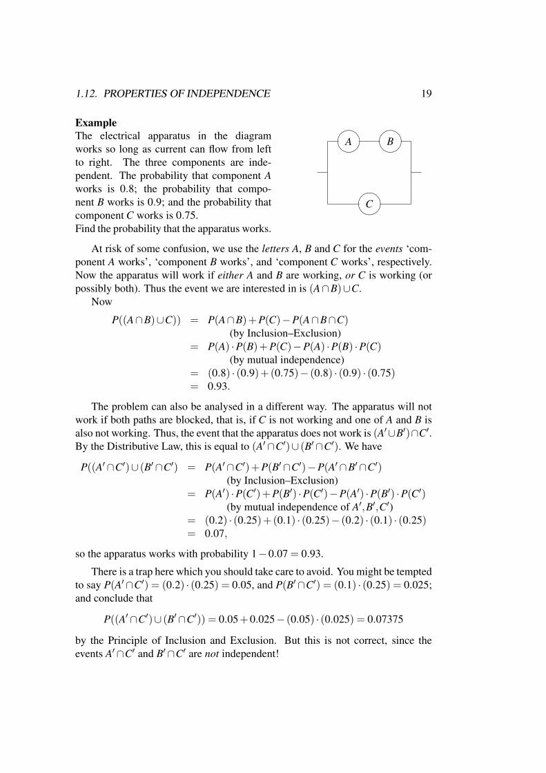
ExampleThe electrical apparatus in the diagramworks so long as current can flow from leftto right. The three components are inde-pendent. The probability that component Aworks is 0.8; the probability that compo-nent B works is 0.9; and the probability thatcomponent C works is 0.75.Find the probability that the apparatus works.
A
B
C
At risk of some confusion, we use the letters A, B and C for the events ‘com-ponent A works’, ‘component B works’, and ‘component C works’, respectively.Now the apparatus will work if either A and B are working, or C is working (orpossibly both). Thus the event we are interested in is (A∩B)∪C.
Now
P((A∩B)∪C)) = P(A∩B)+P(C)−P(A∩B∩C)(by Inclusion–Exclusion)
= P(A) ·P(B)+P(C)−P(A) ·P(B) ·P(C)(by mutual independence)
= (0.8) · (0.9)+(0.75)− (0.8) · (0.9) · (0.75)= 0.93.
The problem can also be analysed in a different way. The apparatus will notwork if both paths are blocked, that is, if C is not working and one of A and B isalso not working. Thus, the event that the apparatus does not work is (A′∪B′)∩C′.By the Distributive Law, this is equal to (A′∩C′)∪ (B′∩C′). We have
P((A′∩C′)∪ (B′∩C′) = P(A′∩C′)+P(B′∩C′)−P(A′∩B′∩C′)(by Inclusion–Exclusion)
= P(A′) ·P(C′)+P(B′) ·P(C′)−P(A′) ·P(B′) ·P(C′)(by mutual independence of A′,B′,C′)
= (0.2) · (0.25)+(0.1) · (0.25)− (0.2) · (0.1) · (0.25)= 0.07,
so the apparatus works with probability 1−0.07 = 0.93.
There is a trap here which you should take care to avoid. You might be temptedto say P(A′∩C′) = (0.2) · (0.25) = 0.05, and P(B′∩C′) = (0.1) · (0.25) = 0.025;and conclude that
P((A′∩C′)∪ (B′∩C′)) = 0.05+0.025− (0.05) · (0.025) = 0.07375
by the Principle of Inclusion and Exclusion. But this is not correct, since theevents A′∩C′ and B′∩C′ are not independent!
20 CHAPTER 1. BASIC IDEAS
Example We can always assume that successive tosses of a coin are mutuallyindependent, even if it is not a fair coin. Suppose that I have a coin which hasprobability 0.6 of coming down heads. I toss the coin three times. What are theprobabilities of getting three heads, two heads, one head, or no heads?
For three heads, since successive tosses are mutually independent, the proba-bility is (0.6)3 = 0.216.
The probability of tails on any toss is 1− 0.6 = 0.4. Now the event ‘twoheads’ can occur in three possible ways, as HHT , HT H, or T HH. Each outcomehas probability (0.6) · (0.6) · (0.4) = 0.144. So the probability of two heads is3 · (0.144) = 0.432.
Similarly the probability of one head is 3 · (0.6) · (0.4)2 = 0.288, and the prob-ability of no heads is (0.4)3 = 0.064.
As a check, we have
0.216+0.432+0.288+0.064 = 1.
1.13 Worked examplesQuestion
(a) You go to the shop to buy a toothbrush. The toothbrushes there are red, blue,green, purple and white. The probability that you buy a red toothbrush isthree times the probability that you buy a green one; the probability that youbuy a blue one is twice the probability that you buy a green one; the proba-bilities of buying green, purple, and white are all equal. You are certain tobuy exactly one toothbrush. For each colour, find the probability that youbuy a toothbrush of that colour.
(b) James and Simon share a flat, so it would be confusing if their toothbrusheswere the same colour. On the first day of term they both go to the shop tobuy a toothbrush. For each of James and Simon, the probability of buyingvarious colours of toothbrush is as calculated in (a), and their choices areindependent. Find the probability that they buy toothbrushes of the samecolour.
(c) James and Simon live together for three terms. On the first day of each termthey buy new toothbrushes, with probabilities as in (b), independently ofwhat they had bought before. This is the only time that they change theirtoothbrushes. Find the probablity that James and Simon have differentlycoloured toothbrushes from each other for all three terms. Is it more likelythat they will have differently coloured toothbrushes from each other for
1.13. WORKED EXAMPLES 21
all three terms or that they will sometimes have toothbrushes of the samecolour?
Solution
(a) Let R,B,G,P,W be the events that you buy a red, blue, green, purple andwhite toothbrush respectively. Let x = P(G). We are given that
P(R) = 3x, P(B) = 2x, P(P) = P(W ) = x.
Since these outcomes comprise the whole sample space, Corollary 2 gives
3x+2x+ x+ x+ x = 1,
so x = 1/8. Thus, the probabilities are 3/8, 1/4, 1/8, 1/8, 1/8 respectively.
(b) Let RB denote the event ‘James buys a red toothbrush and Simon buys a bluetoothbrush’, etc. By independence (given), we have, for example,
P(RR) = (3/8) · (3/8) = 9/64.
The event that the toothbrushes have the same colour consists of the fiveoutcomes RR, BB, GG, PP, WW , so its probability is
P(RR)+P(BB)+P(GG)+P(PP)+P(WW )
=964
+116
+164
+164
+164
=14.
(c) The event ‘different coloured toothbrushes in the ith term’ has probability 3/4(from part (b)), and these events are independent. So the event ‘differentcoloured toothbrushes in all three terms’ has probability
34· 3
4· 3
4=
2764
.
The event ‘same coloured toothbrushes in at least one term’ is the comple-ment of the above, so has probability 1− (27/64) = (37)/(64). So it ismore likely that they will have the same colour in at least one term.
Question There are 24 elephants in a game reserve. The warden tags six of theelephants with small radio transmitters and returns them to the reserve. The nextmonth, he randomly selects five elephants from the reserve. He counts how manyof these elephants are tagged. Assume that no elephants leave or enter the reserve,or die or give birth, between the tagging and the selection; and that all outcomesof the selection are equally likely. Find the probability that exactly two of theselected elephants are tagged, giving the answer correct to 3 decimal places.
22 CHAPTER 1. BASIC IDEAS
Solution The experiment consists of picking the five elephants, not the originalchoice of six elephants for tagging. Let S be the sample space. Then |S |= 24C5.
Let A be the event that two of the selected elephants are tagged. This involveschoosing two of the six tagged elephants and three of the eighteen untagged ones,so |A|= 6C2 · 18C3. Thus
P(A) =6C2 · 18C3
24C5= 0.288
to 3 d.p.
Note: Should the sample should be ordered or unordered? Since the answerdoesn’t depend on the order in which the elephants are caught, an unordered sam-ple is preferable. If you want to use an ordered sample, the calculation is
P(A) =6P2 · 18P3 · 5C2
24P5= 0.288,
since it is necessary to multiply by the 5C2 possible patterns of tagged and un-tagged elephants in a sample of five with two tagged.
Question A couple are planning to have a family. They decide to stop havingchildren either when they have two boys or when they have four children. Sup-pose that they are successful in their plan.
(a) Write down the sample space.
(b) Assume that, each time that they have a child, the probability that it is aboy is 1/2, independent of all other times. Find P(E) and P(F) whereE = “there are at least two girls”, F = “there are more girls than boys”.
Solution (a) S = BB,BGB,GBB,BGGB,GBGB,GGBB,BGGG,GBGG,GGBG,GGGB,GGGG.
(b) E = BGGB,GBGB,GGBB,BGGG,GBGG,GGBG,GGGB,GGGG,F = BGGG,GBGG,GGBG,GGGB,GGGG.
Now we have P(BB) = 1/4, P(BGB) = 1/8, P(BGGB) = 1/16, and similarlyfor the other outcomes. So P(E) = 8/16 = 1/2, P(F) = 5/16.
Chapter 2
Conditional probability
In this chapter we develop the technique of conditional probability to deal withcases where events are not independent.
2.1 What is conditional probability?Alice and Bob are going out to dinner. They toss a fair coin ‘best of three’ todecide who pays: if there are more heads than tails in the three tosses then Alicepays, otherwise Bob pays.
Clearly each has a 50% chance of paying. The sample space is
S = HHH,HHT,HT H,HT T,T HH,T HT,T T H,T T T,
and the events ‘Alice pays’ and ‘Bob pays’ are respectively
A = HHH,HHT,HT H,T HH,B = HT T,T HT,T T H,T T T.
They toss the coin once and the result is heads; call this event E. How shouldwe now reassess their chances? We have
E = HHH,HHT,HT H,HT T,
and if we are given the information that the result of the first toss is heads, then Enow becomes the sample space of the experiment, since the outcomes not in E areno longer possible. In the new experiment, the outcomes ‘Alice pays’ and ‘Bobpays’ are
A∩E = HHH,HHT,HT H,B∩E = HT T.
23
24 CHAPTER 2. CONDITIONAL PROBABILITY
Thus the new probabilities that Alice and Bob pay for dinner are 3/4 and 1/4respectively.
In general, suppose that we are given that an event E has occurred, and wewant to compute the probability that another event A occurs. In general, we can nolonger count, since the outcomes may not be equally likely. The correct definitionis as follows.
Let E be an event with non-zero probability, and let A be any event. Theconditional probability of A given E is defined as
P(A | E) =P(A∩E)
P(E).
Again I emphasise that this is the definition. If you are asked for the definitionof conditional probability, it is not enough to say “the probability of A given thatE has occurred”, although this is the best way to understand it. There is no reasonwhy event E should occur before event A!
Note the vertical bar in the notation. This is P(A | E), not P(A/E) or P(A\E).Note also that the definition only applies in the case where P(E) is not equal
to zero, since we have to divide by it, and this would make no sense if P(E) = 0.To check the formula in our example:
P(A | E) =P(A∩E)
P(E)=
3/81/2
=34,
P(B | E) =P(B∩E)
P(E)=
1/81/2
=14.
It may seem like a small matter, but you should be familiar enough with thisformula that you can write it down without stopping to think about the names ofthe events. Thus, for example,
P(A | B) =P(A∩B)
P(B)
if P(B) 6= 0.
Example A random car is chosen among all those passing through TrafalgarSquare on a certain day. The probability that the car is yellow is 3/100: theprobability that the driver is blonde is 1/5; and the probability that the car isyellow and the driver is blonde is 1/50.
Find the conditional probability that the driver is blonde given that the car isyellow.
2.2. GENETICS 25
Solution: If Y is the event ‘the car is yellow’ and B the event ‘the driver is blonde’,then we are given that P(Y ) = 0.03, P(B) = 0.2, and P(Y ∩B) = 0.02. So
P(B | Y ) =P(B∩Y )
P(Y )=
0.020.03
= 0.667
to 3 d.p. Note that we haven’t used all the information given.
There is a connection between conditional probability and independence:
Proposition 2.1 Let A and B be events with P(B) 6= 0. Then A and B are indepen-dent if and only if P(A | B) = P(A).
Proof The words ‘if and only if’ tell us that we have two jobs to do: we have toshow that if A and B are independent, then P(A | B) = P(A); and that if P(A | B) =P(A), then A and B are independent.
So first suppose that A and B are independent. Remember that this means thatP(A∩B) = P(A) ·P(B). Then
P(A | B) =P(A∩B)
P(B)=
P(A) ·P(B)P(B)
= P(A),
that is, P(A | B) = P(A), as we had to prove.Now suppose that P(A | B) = P(A). In other words,
P(A∩B)P(B)
= P(A),
using the definition of conditional probability. Now clearing fractions gives
P(A∩B) = P(A) ·P(B),
which is just what the statement ‘A and B are independent’ means.
This proposition is most likely what people have in mind when they say ‘Aand B are independent means that B has no effect on A’.
2.2 GeneticsHere is a simplified version of how genes code eye colour, assuming only twocolours of eyes.
Each person has two genes for eye colour. Each gene is either B or b. A childreceives one gene from each of its parents. The gene it receives from its fatheris one of its father’s two genes, each with probability 1/2; and similarly for itsmother. The genes received from father and mother are independent.
If your genes are BB or Bb or bB, you have brown eyes; if your genes are bb,you have blue eyes.
26 CHAPTER 2. CONDITIONAL PROBABILITY
Example Suppose that John has brown eyes. So do both of John’s parents. Hissister has blue eyes. What is the probability that John’s genes are BB?
Solution John’s sister has genes bb, so one b must have come from each parent.Thus each of John’s parents is Bb or bB; we may assume Bb. So the possibilitiesfor John are (writing the gene from his father first)
BB,Bb,bB,bb
each with probability 1/4. (For example, John gets his father’s B gene with prob-ability 1/2 and his mother’s B gene with probability 1/2, and these are indepen-dent, so the probability that he gets BB is 1/4. Similarly for the other combina-tions.)
Let X be the event ‘John has BB genes’ and Y the event ‘John has browneyes’. Then X = BB and Y = BB,Bb,bB. The question asks us to calculateP(X | Y ). This is given by
P(X | Y ) =P(X ∩Y )
P(Y )=
1/43/4
= 1/3.
2.3 The Theorem of Total ProbabilitySometimes we are faced with a situation where we do not know the probability ofan event B, but we know what its probability would be if we were sure that someother event had occurred.
Example An ice-cream seller has to decide whether to order more stock for theBank Holiday weekend. He estimates that, if the weather is sunny, he has a 90%chance of selling all his stock; if it is cloudy, his chance is 60%; and if it rains, hischance is only 20%. According to the weather forecast, the probability of sunshineis 30%, the probability of cloud is 45%, and the probability of rain is 25%. (Weassume that these are all the possible outcomes, so that their probabilities mustadd up to 100%.) What is the overall probability that the salesman will sell all hisstock?
This problem is answered by the Theorem of Total Probability, which we nowstate. First we need a definition. The events A1,A2, . . . ,An form a partition of thesample space if the following two conditions hold:
(a) the events are pairwise disjoint, that is, Ai∩A j = /0 for any pair of events Aiand A j;
(b) A1∪A2∪·· ·∪An = S .
2.3. THE THEOREM OF TOTAL PROBABILITY 27
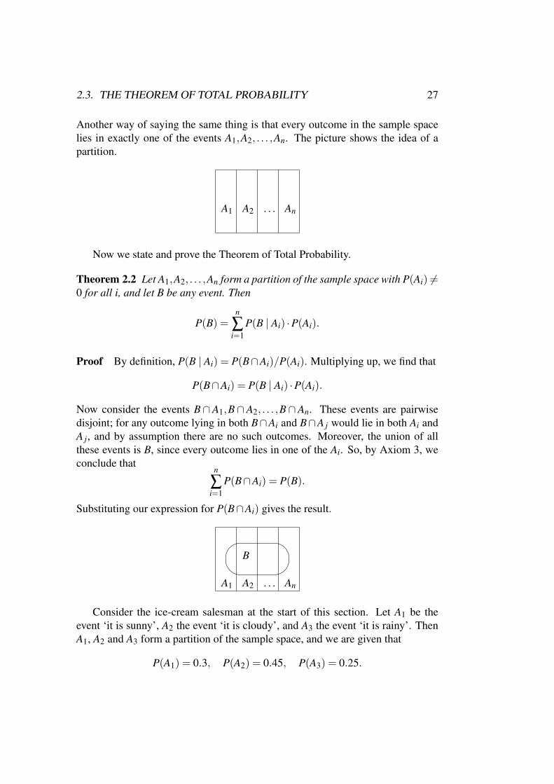
Another way of saying the same thing is that every outcome in the sample spacelies in exactly one of the events A1,A2, . . . ,An. The picture shows the idea of apartition.
A1 A2 . . . An
Now we state and prove the Theorem of Total Probability.
Theorem 2.2 Let A1,A2, . . . ,An form a partition of the sample space with P(Ai) 6=0 for all i, and let B be any event. Then
P(B) =n
∑i=1
P(B | Ai) ·P(Ai).
Proof By definition, P(B | Ai) = P(B∩Ai)/P(Ai). Multiplying up, we find that
P(B∩Ai) = P(B | Ai) ·P(Ai).
Now consider the events B∩ A1,B∩ A2, . . . ,B∩ An. These events are pairwisedisjoint; for any outcome lying in both B∩Ai and B∩A j would lie in both Ai andA j, and by assumption there are no such outcomes. Moreover, the union of allthese events is B, since every outcome lies in one of the Ai. So, by Axiom 3, weconclude that
n
∑i=1
P(B∩Ai) = P(B).
Substituting our expression for P(B∩Ai) gives the result.
A1 A2 . . . An
B
Consider the ice-cream salesman at the start of this section. Let A1 be theevent ‘it is sunny’, A2 the event ‘it is cloudy’, and A3 the event ‘it is rainy’. ThenA1, A2 and A3 form a partition of the sample space, and we are given that
P(A1) = 0.3, P(A2) = 0.45, P(A3) = 0.25.
28 CHAPTER 2. CONDITIONAL PROBABILITY
Let B be the event ‘the salesman sells all his stock’. The other information we aregiven is that
P(B | A1) = 0.9, P(B | A2) = 0.6, P(B | A3) = 0.2.
By the Theorem of Total Probability,
P(B) = (0.9×0.3)+(0.6×0.45)+(0.2×0.25) = 0.59.
You will now realise that the Theorem of Total Probability is really being usedwhen you calculate probabilities by tree diagrams. It is better to get into the habitof using it directly, since it avoids any accidental assumptions of independence.
One special case of the Theorem of Total Probability is very commonly used,and is worth stating in its own right. For any event A, the events A and A′ form apartition of S . To say that both A and A′ have non-zero probability is just to saythat P(A) 6= 0,1. Thus we have the following corollary:
Corollary 2.3 Let A and B be events, and suppose that P(A) 6= 0,1. Then
P(B) = P(B | A) ·P(A)+P(B | A′) ·P(A′).
2.4 Sampling revisitedWe can use the notion of conditional probability to treat sampling problems in-volving ordered samples.
Example I have two red pens, one green pen, and one blue pen. I select twopens without replacement.
(a) What is the probability that the first pen chosen is red?
(b) What is the probability that the second pen chosen is red?
For the first pen, there are four pens of which two are red, so the chance ofselecting a red pen is 2/4 = 1/2.
For the second pen, we must separate cases. Let A1 be the event ‘first pen red’,A2 the event ‘first pen green’ and A3 the event ‘first pen blue’. Then P(A1) = 1/2,P(A2) = P(A3) = 1/4 (arguing as above). Let B be the event ‘second pen red’.
If the first pen is red, then only one of the three remaining pens is red, so thatP(B | A1) = 1/3. On the other hand, if the first pen is green or blue, then two ofthe remaining pens are red, so P(B | A2) = P(B | A3) = 2/3.
2.5. BAYES’ THEOREM 29
By the Theorem of Total Probability,
P(B) = P(B | A1)P(A1)+P(B | A2)P(A2)+P(B | A3)P(A3)= (1/3)× (1/2)+(2/3)× (1/4)+(2/3)× (1/4)= 1/2.
We have reached by a roundabout argument a conclusion which you mightthink to be obvious. If we have no information about the first pen, then the secondpen is equally likely to be any one of the four, and the probability should be 1/2,just as for the first pen. This argument happens to be correct. But, until yourability to distinguish between correct arguments and plausible-looking false onesis very well developed, you may be safer to stick to the calculation that we did.Beware of obvious-looking arguments in probability! Many clever people havebeen caught out.
2.5 Bayes’ TheoremThere is a very big difference between P(A | B) and P(B | A).
Suppose that a new test is developed to identify people who are liable to sufferfrom some genetic disease in later life. Of course, no test is perfect; there will besome carriers of the defective gene who test negative, and some non-carriers whotest positive. So, for example, let A be the event ‘the patient is a carrier’, and Bthe event ‘the test result is positive’.
The scientists who develop the test are concerned with the probabilities thatthe test result is wrong, that is, with P(B | A′) and P(B′ | A). However, a patientwho has taken the test has different concerns. If I tested positive, what is thechance that I have the disease? If I tested negative, how sure can I be that I am nota carrier? In other words, P(A | B) and P(A′ | B′).
These conditional probabilities are related by Bayes’ Theorem:
Theorem 2.4 Let A and B be events with non-zero probability. Then
P(A | B) =P(B | A) ·P(A)
P(B).
The proof is not hard. We have
P(A | B) ·P(B) = P(A∩B) = P(B | A) ·P(A),
using the definition of conditional probability twice. (Note that we need both Aand B to have non-zero probability here.) Now divide this equation by P(B) to getthe result.
30 CHAPTER 2. CONDITIONAL PROBABILITY
If P(A) 6= 0,1 and P(B) 6= 0, then we can use Corollary 17 to write this as
P(A | B) =P(B | A) ·P(A)
P(B | A) ·P(A)+P(B | A′) ·P(A′).
Bayes’ Theorem is often stated in this form.
Example Consider the ice-cream salesman from Section 2.3. Given that he soldall his stock of ice-cream, what is the probability that the weather was sunny?(This question might be asked by the warehouse manager who doesn’t know whatthe weather was actually like.) Using the same notation that we used before, A1is the event ‘it is sunny’ and B the event ‘the salesman sells all his stock’. We areasked for P(A1 | B). We were given that P(B | A1) = 0.9 and that P(A1) = 0.3, andwe calculated that P(B) = 0.59. So by Bayes’ Theorem,
P(A1 | B) =P(B | A1)P(A1)
P(B)=
0.9×0.30.59
= 0.46
to 2 d.p.
Example Consider the clinical test described at the start of this section. Supposethat 1 in 1000 of the population is a carrier of the disease. Suppose also that theprobability that a carrier tests negative is 1%, while the probability that a non-carrier tests positive is 5%. (A test achieving these values would be regarded asvery successful.) Let A be the event ‘the patient is a carrier’, and B the event ‘thetest result is positive’. We are given that P(A) = 0.001 (so that P(A′) = 0.999),and that
P(B | A) = 0.99, P(B | A′) = 0.05.
(a) A patient has just had a positive test result. What is the probability that thepatient is a carrier? The answer is
P(A | B) =P(B | A)P(A)
P(B | A)P(A)+P(B | A′)P(A′)
=0.99×0.001
(0.99×0.001)+(0.05×0.999)
=0.000990.05094
= 0.0194.
(b) A patient has just had a negative test result. What is the probability that thepatient is a carrier? The answer is
P(A | B′) =P(B′ | A)P(A)
P(B′ | A)P(A)+P(B′ | A′)P(A′)

2.6. ITERATED CONDITIONAL PROBABILITY 31
=0.01×0.001
(0.01×0.001)+(0.95×0.999)
=0.000010.94095
= 0.00001.
So a patient with a negative test result can be reassured; but a patient with a posi-tive test result still has less than 2% chance of being a carrier, so is likely to worryunnecessarily.
Of course, these calculations assume that the patient has been selected at ran-dom from the population. If the patient has a family history of the disease, thecalculations would be quite different.
Example 2% of the population have a certain blood disease in a serious form;10% have it in a mild form; and 88% don’t have it at all. A new blood test isdeveloped; the probability of testing positive is 9/10 if the subject has the seriousform, 6/10 if the subject has the mild form, and 1/10 if the subject doesn’t havethe disease.
I have just tested positive. What is the probability that I have the serious formof the disease?
Let A1 be ‘has disease in serious form’, A2 be ‘has disease in mild form’, andA3 be ‘doesn’t have disease’. Let B be ‘test positive’. Then we are given that A1,A2, A3 form a partition and
P(A1) = 0.02 P(A2) = 0.1 P(A3) = 0.88P(B | A1) = 0.9 P(B | A2) = 0.6 P(B | A3) = 0.1
Thus, by the Theorem of Total Probability,
P(B) = 0.9×0.02+0.6×0.1+0.1×0.88 = 0.166,
and then by Bayes’ Theorem,
P(A1 | B) =P(B | A1)P(A1)
P(B)=
0.9×0.020.166
= 0.108
to 3 d.p.
2.6 Iterated conditional probabilityThe conditional probability of C, given that both A and B have occurred, is justP(C | A∩B). Sometimes instead we just write P(C | A,B). It is given by
P(C | A,B) =P(C∩A∩B)
P(A∩B),
32 CHAPTER 2. CONDITIONAL PROBABILITY
soP(A∩B∩C) = P(C | A,B)P(A∩B).
Now we also haveP(A∩B) = P(B | A)P(A),
so finally (assuming that P(A∩B) 6= 0), we have
P(A∩B∩C) = P(C | A,B)P(B | A)P(A).
This generalises to any number of events:
Proposition 2.5 Let A1, . . . ,An be events. Suppose that P(A1 ∩ ·· · ∩An−1) 6= 0.Then
P(A1∩A2∩·· ·∩An) = P(An | A1, . . . ,An−1) · · ·P(A2 | A1)P(A1).
We apply this to the birthday paradox.The birthday paradox is the following statement:
If there are 23 or more people in a room, then the chances are betterthan even that two of them have the same birthday.
To simplify the analysis, we ignore 29 February, and assume that the other 365days are all equally likely as birthdays of a random person. (This is not quite truebut not inaccurate enough to have much effect on the conclusion.) Suppose thatwe have n people p1, p2, . . . , pn. Let A2 be the event ‘p2 has a different birthdayfrom p1’. Then P(A2) = 1− 1
365 , since whatever p1’s birthday is, there is a 1 in365 chance that p2 will have the same birthday.
Let A3 be the event ‘p3 has a different birthday from p1 and p2’. It is notstraightforward to evaluate P(A3), since we have to consider whether p1 and p2have the same birthday or not. (See below). But we can calculate that P(A3 |A2) = 1− 2
365 , since if A2 occurs then p1 and p2 have birthdays on different days,and A3 will occur only if p3’s birthday is on neither of these days. So
P(A2∩A3) = P(A2)P(A3 | A2) = (1− 1365)(1− 2
365).
What is A2 ∩A3? It is simply the event that all three people have birthdays ondifferent days.
Now this process extends. If Ai denotes the event ‘pi’s birthday is not on thesame day as any of p1, . . . , pi−1’, then
P(Ai | A1, . . . ,Ai−1) = 1− i−1365 ,
2.6. ITERATED CONDITIONAL PROBABILITY 33
and so by Proposition 2.5,
P(A1∩·· ·∩Ai) = (1− 1365)(1− 2
365) · · ·(1− i−1365 ).
Call this number qi; it is the probability that all of the people p1, . . . , pi havetheir birthdays on different days.
The numbers qi decrease, since at each step we multiply by a factor less than 1.So there will be some value of n such that
qn−1 > 0.5, qn ≤ 0.5,
that is, n is the smallest number of people for which the probability that they allhave different birthdays is less than 1/2, that is, the probability of at least onecoincidence is greater than 1/2.
By calculation, we find that q22 = 0.5243, q23 = 0.4927 (to 4 d.p.); so 23people are enough for the probability of coincidence to be greater than 1/2.
Now return to a question we left open before. What is the probability of theevent A3? (This is the event that p3 has a different birthday from both p1 and p2.)
If p1 and p2 have different birthdays, the probability is 1− 2365 : this is the
calculation we already did. On the other hand, if p1 and p2 have the same birthday,then the probability is 1− 1
365 . These two numbers are P(A3 | A2) and P(A3 | A′2)respectively. So, by the Theorem of Total Probability,
P(A3) = P(A3 | A2)P(A2)+P(A3 | A′2)P(A′2)= (1− 2
365)(1− 1365)+(1− 1
365) 1365
= 0.9945
to 4 d.p.
Problem How many people would you need to pick at random to ensure thatthe chance of two of them being born in the same month are better than even?
Assuming all months equally likely, if Bi is the event that pi is born in a dif-ferent month from any of p1, . . . , pi−1, then as before we find that
P(Bi | B1, · · · ,Bi−1) = 1− i−112 ,
soP(B1∩·· ·∩Bi) = (1− 1
12)(1− 212)(1− i−1
12 ).
We calculate that this probability is
(11/12)× (10/12)× (9/12) = 0.5729
34 CHAPTER 2. CONDITIONAL PROBABILITY
for i = 4 and
(11/12)× (10/12)× (9/12)× (8/12) = 0.3819
for i = 5. So, with five people, it is more likely that two will have the same birthmonth.
A true story. Some years ago, in a probability class with only ten students, thelecturer started discussing the Birthday Paradox. He said to the class, “I bet thatno two people in the room have the same birthday”. He should have been on safeground, since q11 = 0.859. (Remember that there are eleven people in the room!)However, a student in the back said “I’ll take the bet”, and after a moment all theother students realised that the lecturer would certainly lose his wager. Why?
(Answer in the next chapter.)
2.7 Worked examplesQuestion Each person has two genes for cystic fibrosis. Each gene is either Nor C. Each child receives one gene from each parent. If your genes are NN or NCor CN then you are normal; if they are CC then you have cystic fibrosis.
(a) Neither of Sally’s parents has cystic fibrosis. Nor does she. However, Sally’ssister Hannah does have cystic fibrosis. Find the probability that Sally hasat least one C gene (given that she does not have cystic fibrosis).
(b) In the general population the ratio of N genes to C genes is about 49 to 1.You can assume that the two genes in a person are independent. Harry doesnot have cystic fibrosis. Find the probability that he has at least one C gene(given that he does not have cystic fibrosis).
(c) Harry and Sally plan to have a child. Find the probability that the child willhave cystic fibrosis (given that neither Harry nor Sally has it).
Solution During this solution, we will use a number of times the following prin-ciple. Let A and B be events with A ⊆ B. Then A∩B = A, and so
P(A | B) =P(A∩B)
P(B)=
P(A)P(B)
.
(a) This is the same as the eye colour example discussed earlier. We are giventhat Sally’s sister has genes CC, and one gene must come from each parent. But
2.7. WORKED EXAMPLES 35
neither parent is CC, so each parent is CN or NC. Now by the basic rules ofgenetics, all the four combinations of genes for a child of these parents, namelyCC,CN,NC,NN, will have probability 1/4.
If S1 is the event ‘Sally has at least one C gene’, then S1 = CN,NC,CC; andif S2 is the event ‘Sally does not have cystic fibrosis’, then S2 = CN,NC,NN.Then
P(S1 | S2) =P(S1∩S2)
P(S2)=
2/43/4
=23.
(b) We know nothing specific about Harry, so we assume that his genes arerandomly and independently selected from the population. We are given that theprobability of a random gene being C or N is 1/50 and 49/50 respectively. Thenthe probabilities of Harry having genes CC, CN, NC, NN are respectively (1/50)2,(1/50) · (49/50), (49/50) · (1/50), and (49/50)2, respectively. So, if H1 is theevent ‘Harry has at least one C gene’, and H2 is the event ‘Harry does not havecystic fibrosis’, then
P(H1 | H2) =P(H1∩H2)
P(H2)=
(49/2500)+(49/2500)(49/2500)+(49/2500)+(2401/2500)
=2
51.
(c) Let X be the event that Harry’s and Sally’s child has cystic fibrosis. As in(a), this can only occur if Harry and Sally both have CN or NC genes. That is,X ⊆ S3∩H3, where S3 = S1∩ S2 and H3 = H1∩H2. Now if Harry and Sally areboth CN or NC, these genes pass independently to the baby, and so
P(X | S3∩H3) =P(X)
P(S3∩H3)=
14.
(Remember the principle that we started with!)We are asked to find P(X | S2 ∩H2), in other words (since X ⊆ S3 ∩H3 ⊆
S2∩H2),P(X)
P(S2∩H2).
Now Harry’s and Sally’s genes are independent, so
P(S3∩H3) = P(S3) ·P(H3),P(S2∩H2) = P(S2) ·P(H2).
Thus,
P(X)P(S2∩H2)
=P(X)
P(S3∩H3)· P(S3∩H3)
P(S2∩H2)
36 CHAPTER 2. CONDITIONAL PROBABILITY
=14· P(S1∩S2)
P(S2)· P(H1∩H2)
P(H2)
=14·P(S1 | S2) ·P(H1 | H2)
=14· 2
3· 2
51
=1
153.
I thank Eduardo Mendes for pointing out a mistake in my previous solution tothis problem.
Question The Land of Nod lies in the monsoon zone, and has just two seasons,Wet and Dry. The Wet season lasts for 1/3 of the year, and the Dry season for 2/3of the year. During the Wet season, the probability that it is raining is 3/4; duringthe Dry season, the probability that it is raining is 1/6.
(a) I visit the capital city, Oneirabad, on a random day of the year. What is theprobability that it is raining when I arrive?
(b) I visit Oneirabad on a random day, and it is raining when I arrive. Given thisinformation, what is the probability that my visit is during the Wet season?
(c) I visit Oneirabad on a random day, and it is raining when I arrive. Given thisinformation, what is the probability that it will be raining when I return toOneirabad in a year’s time?
(You may assume that in a year’s time the season will be the same as today but,given the season, whether or not it is raining is independent of today’s weather.)
Solution (a) Let W be the event ‘it is the wet season’, D the event ‘it is the dryseason’, and R the event ‘it is raining when I arrive’. We are given that P(W ) =1/3, P(D) = 2/3, P(R |W ) = 3/4, P(R | D) = 1/6. By the ToTP,
P(R) = P(R |W )P(W )+P(R | D)P(D)= (3/4) · (1/3)+(1/6) · (2/3) = 13/36.
(b) By Bayes’ Theorem,
P(W | R) =P(R |W )P(W )
P(R)=
(3/4) · (1/3)13/36
=913
.
2.7. WORKED EXAMPLES 37
(c) Let R′ be the event ‘it is raining in a year’s time’. The information we aregiven is that P(R∩R′ |W ) = P(R |W )P(R′ |W ) and similarly for D. Thus
P(R∩R′) = P(R∩R′ |W )P(W )+P(R∩R′ | D)P(D)
= (3/4)2 · (1/3)+(1/6)2 · (2/3) =89432
,
and so
P(R′ | R) =P(R∩R′)
P(R)=
89/43213/36
=89
156.

38 CHAPTER 2. CONDITIONAL PROBABILITY
Chapter 3
Random variables
In this chapter we define random variables and some related concepts such asprobability mass function, expected value, variance, and median; and look at someparticularly important types of random variables including the binomial, Poisson,and normal.
3.1 What are random variables?The Holy Roman Empire was, in the words of the historian Voltaire, “neither holy,nor Roman, nor an empire”. Similarly, a random variable is neither random nor avariable:
A random variable is a function defined on a sample space.
The values of the function can be anything at all, but for us they will always benumbers. The standard abbreviation for ‘random variable’ is r.v.
Example I select at random a student from the class and measure his or herheight in centimetres.
Here, the sample space is the set of students; the random variable is ‘height’,which is a function from the set of students to the real numbers: h(S) is the heightof student S in centimetres. (Remember that a function is nothing but a rule forassociating with each element of its domain set an element of its target or rangeset. Here the domain set is the sample space S , the set of students in the class, andthe target space is the set of real numbers.)
Example I throw a six-sided die twice; I am interested in the sum of the twonumbers. Here the sample space is
S = (i, j) : 1 ≤ i, j ≤ 6,
39
40 CHAPTER 3. RANDOM VARIABLES
and the random variable F is given by F(i, j) = i + j. The target set is the set2,3, . . . ,12.
The two random variables in the above examples are representatives of the twotypes of random variables that we will consider. These definitions are not quiteprecise, but more examples should make the idea clearer.
A random variable F is discrete if the values it can take are separated by gaps.For example, F is discrete if it can take only finitely many values (as in the secondexample above, where the values are the integers from 2 to 12), or if the values ofF are integers (for example, the number of nuclear decays which take place in asecond in a sample of radioactive material – the number is an integer but we can’teasily put an upper limit on it.)
A random variable is continuous if there are no gaps between its possiblevalues. In the first example, the height of a student could in principle be any realnumber between certain extreme limits. A random variable whose values rangeover an interval of real numbers, or even over all real numbers, is continuous.
One could concoct random variables which are neither discrete nor continuous(e.g. the possible, values could be 1, 2, 3, or any real number between 4 and 5),but we will not consider such random variables.
We begin by considering discrete random variables.
3.2 Probability mass functionLet F be a discrete random variable. The most basic question we can ask is: givenany value a in the target set of F , what is the probability that F takes the value a?In other words, if we consider the event
A = x ∈ S : F(x) = a
what is P(A)? (Remember that an event is a subset of the sample space.) Sinceevents of this kind are so important, we simplify the notation: we write
P(F = a)
in place ofP(x ∈ S : F(x) = a).
(There is a fairly common convention in probability and statistics that randomvariables are denoted by capital letters and their values by lower-case letters. Infact, it is quite common to use the same letter in lower case for a value of therandom variable; thus, we would write P(F = f ) in the above example. Butremember that this is only a convention, and you are not bound to it.)

3.3. EXPECTED VALUE AND VARIANCE 41
The probability mass function of a discrete random variable F is the function,formula or table which gives the value of P(F = a) for each element a in the targetset of F . If F takes only a few values, it is convenient to list it in a table; otherwisewe should give a formula if possible. The standard abbreviation for ‘probabilitymass function’ is p.m.f.
Example I toss a fair coin three times. The random variable X gives the numberof heads recorded. The possible values of X are 0,1,2,3, and its p.m.f. is
a 0 1 2 3P(X = a) 1
838
38
18
For the sample space is HHH,HHT,HT H,HT T,T HH,T HT,T T H,T T T, andeach outcome is equally likely. The event X = 1, for example, when written as aset of outcomes, is equal to HT T,T HT,T T H, and has probability 3/8.
Two random variables X and Y are said to have the same distribution if thevalues they take and their probability mass functions are equal. We write X ∼ Yin this case.
In the above example, if Y is the number of tails recorded during the experi-ment, then X and Y have the same distribution, even though their actual values aredifferent (indeed, Y = 3−X).
3.3 Expected value and varianceLet X be a discrete random variable which takes the values a1, . . . ,an. The ex-pected value or mean of X is the number E(X) given by the formula
E(X) =n
∑i=1
aiP(X = ai).
That is, we multiply each value of X by the probability that X takes that value,and sum these terms. The expected value is a kind of ‘generalised average’: ifeach of the values is equally likely, so that each has probability 1/n, then E(X) =(a1 + · · ·+an)/n, which is just the average of the values.
There is an interpretation of the expected value in terms of mechanics. If weput a mass pi on the axis at position ai for i = 1, . . . ,n, where pi = P(X = ai), thenthe centre of mass of all these masses is at the point E(X).
If the random variable X takes infinitely many values, say a1,a2,a3, . . ., thenwe define the expected value of X to be the infinite sum
E(X) =∞
∑i=1
aiP(X = ai).
42 CHAPTER 3. RANDOM VARIABLES
Of course, now we have to worry about whether this means anything, that is,whether this infinite series is convergent. This is a question which is discussedat great length in analysis. We won’t worry about it too much. Usually, discreterandom variables will only have finitely many values; in the few examples weconsider where there are infinitely many values, the series will usually be a ge-ometric series or something similar, which we know how to sum. In the proofsbelow, we assume that the number of values is finite.
The variance of X is the number Var(X) given by
Var(X) = E(X2)−E(X)2.
Here, X2 is just the random variable whose values are the squares of the values ofX . Thus
E(X2) =n
∑i=1
a2i P(X = ai)
(or an infinite sum, if necessary). The next theorem shows that, if E(X) is a kindof average of the values of X , then Var(X) is a measure of how spread-out thevalues are around their average.
Proposition 3.1 Let X be a discrete random variable with E(X) = µ. Then
Var(X) = E((X −µ)2) =n
∑i=1
(ai−µ)2P(X = ai).
For the second term is equal to the third by definition, and the third isn
∑i=1
(ai−µ)2P(X = ai)
=n
∑i=1
(a2i −2µai +µ2)P(X = ai)
=
(n
∑i=1
a2i P(X = ai)
)−2µ
(n
∑i=1
aiP(X = ai)
)+µ2
(n
∑i=1
P(X = ai)
).
(What is happening here is that the entire sum consists of n rows with three termsin each row. We add it up by columns instead of by rows, getting three parts withn terms in each part.) Continuing, we find
E((X −µ)2) = E(X2)−2µE(X)+µ2
= E(X2)−E(X)2,
and we are done. (Remember that E(X) = µ, and that ∑ni=1 P(X = ai) = 1 since
the events X = ai form a partition.)

3.4. JOINT P.M.F. OF TWO RANDOM VARIABLES 43
Some people take the conclusion of this proposition as the definition of vari-ance.
Example I toss a fair coin three times; X is the number of heads. What are theexpected value and variance of X?
E(X) = 0× (1/8)+1× (3/8)+2× (3/8)+3× (1/8) = 3/2,
Var(X) = 02× (1/8)+12× (3/8)+22× (3/8)+32× (1/8)− (3/2)2 = 3/4.
If we calculate the variance using Proposition 3.1, we get
Var(X) =(−3
2
)2
× 18
+(−1
2
)2
× 38
+(
12
)2
× 38
+(
32
)2
× 18
=34.
Two properties of expected value and variance can be used as a check on yourcalculations.
• The expected value of X always lies between the smallest and largest valuesof X .
• The variance of X is never negative. (For the formula in Proposition 3.1 isa sum of terms, each of the form (ai− µ)2 (a square, hence non-negative)times P(X = ai) (a probability, hence non-negative).
3.4 Joint p.m.f. of two random variablesLet X be a random variable taking the values a1, . . . ,an, and let Y be a randomvariable taking the values b1, . . . ,bm. We say that X and Y are independent if, forany possible values i and j, we have
P(X = ai,Y = b j) = P(X = ai) ·P(Y = b j).
Here P(X = ai,Y = b j) means the probability of the event that X takes the valueai and Y takes the value b j. So we could re-state the definition as follows:
The random variables X and Y are independent if, for any value ai ofX and any value b j of Y , the events X = ai and Y = b j are independent(events).
Note the difference between ‘independent events’ and ‘independent random vari-ables’.
44 CHAPTER 3. RANDOM VARIABLES
Example In Chapter 2, we saw the following: I have two red pens, one greenpen, and one blue pen. I select two pens without replacement. Then the events‘exactly one red pen selected’ and ‘exactly one green pen selected’ turned out tobe independent. Let X be the number of red pens selected, and Y the number ofgreen pens selected. Then
P(X = 1,Y = 1) = P(X = 1) ·P(Y = 1).
Are X and Y independent random variables?No, because P(X = 2) = 1/6, P(Y = 1) = 1/2, but P(X = 2,Y = 1) = 0 (it is
impossible to have two red and one green in a sample of two).
On the other hand, if I roll a die twice, and X and Y are the numbers that comeup on the first and second throws, then X and Y will be independent, even if thedie is not fair (so that the outcomes are not all equally likely).
If we have more than two random variables (for example X ,Y,Z), we say thatthey are mutually independent if the events that the random variables take specificvalues (for example, X = a, Y = b, Z = c) are mutually independent. (You maywant to revise the material on mutually independent events.)
What about the expected values of random variables? For expected value, it iseasy, but for variance it helps if the variables are independent:
Theorem 3.2 Let X and Y be random variables.
(a) E(X +Y ) = E(X)+E(Y ).
(b) If X and Y are independent, then Var(X +Y ) = Var(X)+Var(Y ).
We will see the proof later.
If two random variables X and Y are not independent, then knowing the p.m.f.of each variable does not tell the whole story. The joint probability mass function(or joint p.m.f.) of X and Y is the table giving, for each value ai of X and eachvalue b j of Y , the probability that X = ai and Y = b j. We arrange the table sothat the rows correspond to the values of X and the columns to the values of Y .Note that summing the entries in the row corresponding to the value ai gives theprobability that X = ai; that is, the row sums form the p.m.f. of X . Similarly thecolumn sums form the p.m.f. of Y . (The row and column sums are sometimescalled the marginal distributions or marginals.)
In particular, X and Y are independent r.v.s if and only if each entry of thetable is equal to the product of its row sum and its column sum.
3.4. JOINT P.M.F. OF TWO RANDOM VARIABLES 45
Example I have two red pens, one green pen, and one blue pen, and I choosetwo pens without replacement. Let X be the number of red pens that I choose andY the number of green pens. Then the joint p.m.f. of X and Y is given by thefollowing table:
Y0 1
0 0 16
X 1 13
13
2 16 0
The row and column sums give us the p.m.f.s for X and Y :
a 0 1 2
P(X = a) 16
23
16
b 0 1
P(Y = b) 12
12
Now we give the proof of Theorem 3.2.We consider the joint p.m.f. of X and Y . The random variable X +Y takes the
values ai + b j for i = 1, . . . ,n and j = 1, . . . ,m. Now the probability that it takesa given value ck is the sum of the probabilities P(X = ai,Y = b j) over all i and jsuch that ai +b j = ck. Thus,
E(X +Y ) = ∑k
ckP(X +Y = ck)
=n
∑i=1
m
∑j=1
(ai +b j)P(X = ai,Y = b j)
=
(n
∑i=1
ai
m
∑j=1
P(X = ai,Y = b j)
)+
(m
∑j=1
b j
n
∑i=1
P(X = ai,Y = b j)
).
Now ∑mj=1 P(X = ai,Y = b j) is a row sum of the joint p.m.f. table, so is equal to
P(X = ai), and similarly ∑ni=1 P(X = ai,Y = b j) is a column sum and is equal to
P(Y = b j). So
E(X +Y ) =n
∑i=1
aiP(X = ai)+m
∑j=1
b jP(Y = b j)
= E(X)+E(Y ).
The variance is a bit trickier. First we calculate
E((X +Y )2) = E(X2 +2XY +Y 2) = E(X2)+2E(XY )+E(Y 2),
46 CHAPTER 3. RANDOM VARIABLES
using part (a) of the Theorem. We have to consider the term E(XY ). For this, wehave to make the assumption that X and Y are independent, that is,
P(X = a1,Y = b j) = P(X = ai) ·P(Y = b j).
As before, we have
E(XY ) =n
∑i=1
m
∑j=1
aib jP(X = ai,Y = b j)
=n
∑i=1
n
∑j=1
aib jP(X = ai)P(Y = b j)
=
(n
∑i=1
aiP(X = ai)
)·
(m
∑j=1
b jP(Y = b j)
)= E(X) ·E(Y ).
So
Var(X +Y ) = E((X +Y )2)− (E(X +Y ))2
= (E(X2)+2E(XY )+E(Y 2))− (E(X)2 +2E(X)E(Y )+E(Y )2)= (E(X2)−E(X)2)+2(E(XY )−E(X)E(Y ))+(E(Y 2)−E(Y )2)= Var(X)+Var(Y ).
To finish this section, we consider constant random variables. (If the thoughtof a ‘constant variable’ worries you, remember that a random variable is not avariable at all but a function, and there is nothing amiss with a constant function.)
Proposition 3.3 Let C be a constant random variable with value c. Let X be anyrandom variable.
(a) E(C) = c, Var(C) = 0.
(b) E(X + c) = E(X)+ c, Var(X + c) = Var(X).
(c) E(cX) = cE(X), Var(cX) = c2 Var(X).
Proof (a) The random variable C takes the single value c with P(C = c) = 1. SoE(C) = c ·1 = c. Also,
Var(C) = E(C2)−E(C)2 = c2− c2 = 0.
(For C2 is a constant random variable with value c2.)
3.5. SOME DISCRETE RANDOM VARIABLES 47
(b) This follows immediately from Theorem 3.2, once we observe that theconstant random variable C and any random variable X are independent. (This istrue because P(X = a,C = c) = P(X = a) ·1.) Then
E(X + c) = E(X)+E(C) = E(X)+ c,Var(X + c) = Var(X)+Var(C) = Var(X).
(c) If a1, . . . ,an are the values of X , then ca1, . . . ,can are the values of cX , andP(cX = cai) = P(x = ai). So
E(cX) =n
∑i=1
caiP(cX = cai)
= cn
∑i=1
aiP(X = ai)
= cE(X).
Then
Var(cX) = E(c2X2)−E(cX)2
= c2E(X2)− (cE(X))2
= c2(E(X2)−E(X)2)= c2 Var(X).
3.5 Some discrete random variablesWe now look at five types of discrete random variables, each depending on one ormore parameters. We describe for each type the situations in which it arises, andgive the p.m.f., the expected value, and the variance. If the variable is tabulatedin the New Cambridge Statistical Tables, we give the table number, and someexamples of using the tables. You should have a copy of the tables to follow theexamples.
A summary of this information is given in Appendix B.Before we begin, a comment on the New Cambridge Statistical Tables. They
don’t give the probability mass function (or p.m.f.), but a closely related functioncalled the cumulative distribution function. It is defined for a discrete randomvariable as follows.
Let X be a random variable taking values a1,a2, . . . ,an. We assume that theseare arranged in ascending order: a1 < a2 < · · ·< an. The cumulative distributionfunction, or c.d.f., of X is given by
FX(ai) = P(X ≤ ai).
48 CHAPTER 3. RANDOM VARIABLES
We see that it can be expressed in terms of the p.m.f. of X as follows:
FX(ai) = P(X = a1)+ · · ·+P(X = ai) =i
∑j=1
P(X = a j).
In the other direction, we cn recover the p.m.f. from the c.d.f.:
P(X = ai) = FX(ai)−FX(ai−1).
We won’t use the c.d.f. of a discrete random variable except for looking upthe tables. It is much more important for continuous random variables!
Bernoulli random variable Bernoulli(p)
A Bernoulli random variable is the simplest type of all. It only takes two values,0 and 1. So its p.m.f. looks as follows:
x 0 1P(X = x) q p
Here, p is the probability that X = 1; it can be any number between 0 and 1.Necessarily q (the probability that X = 0) is equal to 1− p. So p determineseverything.
For a Bernoulli random variable X , we sometimes describe the experiment asa ‘trial’, the event X = 1 as‘success’, and the event X = 0 as ‘failure’.
For example, if a biased coin has probability p of coming down heads, thenthe number of heads that we get when we toss the coin once is a Bernoulli(p)random variable.
More generally, let A be any event in a probability space S . With A, we asso-ciate a random variable IA (remember that a random variable is just a function onS ) by the rule
IA(s) =1 if s ∈ A;
0 if s /∈ A.The random variable IA is called the indicator variable of A, because its valueindicates whether or not A occurred. It is a Bernoulli(p) random variable, wherep = P(A). (The event IA = 1 is just the event A.) Some people write 11A instead ofIA.
Calculation of the expected value and variance of a Bernoulli random variableis easy. Let X ∼ Bernoulli(p). (Remember that ∼ means “has the same p.m.f.as”.)
E(X) = 0 ·q+1 · p = p;
Var(X) = 02 ·q+12 · p− p2 = p− p2 = pq.
(Remember that q = 1− p.)
3.5. SOME DISCRETE RANDOM VARIABLES 49
Binomial random variable Bin(n, p)
Remember that for a Bernoulli random variable, we describe the event X = 1 as a‘success’. Now a binomial random variable counts the number of successes in nindependent trials each associated with a Bernoulli(p) random variable.
For example, suppose that we have a biased coin for which the probability ofheads is p. We toss the coin n times and count the number of heads obtained. Thisnumber is a Bin(n, p) random variable.
A Bin(n, p) random variable X takes the values 0,1,2, . . . ,n, and the p.m.f. ofX is given by
P(X = k) = nCkqn−k pk
for k = 0,1,2, . . . ,n, where q = 1− p. This is because there are nCk different waysof obtaining k heads in a sequence of n throws (the number of choices of the kpositions in which the heads occur), and the probability of getting k heads andn− k tails in a particular order is qn−k pk.
Note that we have given a formula rather than a table here. For small valueswe could tabulate the results; for example, for Bin(4, p):
k 0 1 2 3 4
P(X = k) q4 4q3 p 6q2 p2 4qp3 p4
Note: when we add up all the probabilities in the table, we getn
∑k=0
nCkqn−k pk = (q+ p)n = 1,
as it should be: here we used the binomial theorem
(x+ y)n =n
∑k=0
nCkxn−kyk.
(This argument explains the name of the binomial random variable!)If X ∼ Bin(n, p), then
E(X) = np, Var(X) = npq.
There are two ways to prove this, an easy way and a harder way. The easy wayonly works for the binomial, but the harder way is useful for many random vari-ables. However, you can skip it if you wish: I have set it in smaller type for thisreason.
Here is the easy method. We have a coin with probability p of coming downheads, and we toss it n times and count the number X of heads. Then X is ourBin(n, p) random variable. Let Xk be the random variable defined by
Xk =
1 if we get heads on the kth toss,0 if we get tails on the kth toss.
50 CHAPTER 3. RANDOM VARIABLES
In other words, Xi is the indicator variable of the event ‘heads on the kth toss’.Now we have
X = X1 +X2 + · · ·+Xn
(can you see why?), and X1, . . . ,Xn are independent Bernoulli(p) random variables(since they are defined by different tosses of a coin). So, as we saw earlier, E(Xi) =p, Var(Xi) = pq. Then, by Theorem 21, since the variables are independent, wehave
E(X) = p+ p+ · · ·+ p = np,
Var(X) = pq+ pq+ · · ·+ pq = npq.
The other method uses a gadget called the probability generating function. We only use ithere for calculating expected values and variances, but if you learn more probability theory youwill see other uses for it. Let X be a random variable whose values are non-negative integers. (Wedon’t insist that it takes all possible values; this method is fine for the binomial Bin(n, p), whichtakes values between 0 and n. To save space, we write pk for the probability P(X = k). Now theprobability generating function of X is the power series
GX (x) = ∑ pkxk.
(The sum is over all values k taken by X .)We use the notation [F(x)]x=1 for the result of substituting x = 1 in the series F(x).
Proposition 3.4 Let GX (x) be the probability generating function of a random variable X. Then
(a) [GX (x)]x=1 = 1;
(b) E(X) =[ d
dx GX (x)]
x=1;
(c) Var(X) =[
d2
dx2 GX (x)]
x=1+E(X)−E(X)2.
Part (a) is just the statement that probabilities add up to 1: when we substitute x = 1 in thepower series for GX (x) we just get ∑ pk.
For part (b), when we differentiate the series term-by-term (you will learn later in Analysisthat this is OK), we get
ddx
GX (x) = ∑kpkxk−1.
Now putting x = 1 in this series we get
∑kpk = E(X).
For part (c), differentiating twice gives
d2
dx2 GX (x) = ∑k(k−1)pkxk−2.
Now putting x = 1 in this series we get
∑k(k−1)pk = ∑k2 pk−∑kpk = E(X2)−E(X).
Adding E(X) and subtracting E(X)2 gives E(X2)−E(X)2, which by definition is Var(X).

3.5. SOME DISCRETE RANDOM VARIABLES 51
Now let us appply this to the binomial random variable X ∼ Bin(n, p). We have
pk = P(X = k) = nCkqn−k pk,
so the probability generating function is
n
∑k=0
nCkqn−k pkxk = (q+ px)n,
by the Binomial Theorem. Putting x = 1 gives (q+ p)n = 1, in agreement with Proposition 3.4(a).Differentiating once, using the Chain Rule, we get np(q+ px)n−1. Putting x = 1 we find that
E(X) = np.
Differentiating again, we get n(n−1)p2(q+ px)n−2. Putting x = 1 gives n(n−1)p2. Now addingE(X)−E(X)2, we get
Var(X) = n(n−1)p2 +np−n2 p2 = np−np2 = npq.
The binomial random variable is tabulated in Table 1 of the Cambridge Statis-tical Tables [1]. As explained earlier, the tables give the cumulative distributionfunction.
For example, suppose that the probability that a certain coin comes downheads is 0.45. If the coin is tossed 15 times, what is the probability of five orfewer heads? Turning to the page n = 15 in Table 1 and looking at the row 0.45,you read off the answer 0.2608. What is the probability of exactly five heads? Thisis P(5 or fewer)−P(4 or fewer), and from tables the answer is 0.2608−0.1204 =0.1404.
The tables only go up to p = 0.5. For larger values of p, use the fact that thenumber of failures in Bin(n, p) is equal to the number of successes in Bin(n,1−p). So the probability of five heads in 15 tosses of a coin with p = 0.55 is 0.9745−0.9231 = 0.0514.
Another interpretation of the binomial random variable concerns sampling.Suppose that we have N balls in a box, of which M are red. We sample n ballsfrom the box with replacement; let the random variable X be the number of redballs in the sample. What is the distribution of X? Since each ball has probabilityM/N of being red, and different choices are independent, X ∼ Bin(n, p), wherep = M/N is the proportion of red balls in the sample.
What about sampling without replacement? This leads us to our next randomvariable:
Hypergeometric random variable Hg(n,M,N)
Suppose that we have N balls in a box, of which M are red. We sample n ballsfrom the box without replacement. Let the random variable X be the number of
52 CHAPTER 3. RANDOM VARIABLES
red balls in the sample. Such an X is called a hypergeometric random variableHg(n,M,N).
The random variable X can take any of the values 0,1,2, . . . ,n. Its p.m.f. isgiven by the formula
P(X = k) =MCk ·N−MCn−k
NCn.
For the number of samples of n balls from N is NCn; the number of ways ofchoosing k of the M red balls and n−k of the N−M others is MCk ·N−MCn−k; andall choices are equally likely.
The expected value and variance of a hypergeometric random variable are asfollows (we won’t go into the proofs):
E(X) = n(
MN
), Var(X) = n
(MN
)(N−M
N
)(N−nN−1
).
You should compare these to the values for a binomial random variable. If welet p = M/N be the proportion of red balls in the hat, then E(X) = np, and Var(X)is equal to npq multiplied by a ‘correction factor’ (N−n)/(N−1).
In particular, if the numbers M and N −M of red and non-red balls in thehat are both very large compared to the size n of the sample, then the differencebetween sampling with and without replacement is very small, and indeed the‘correction factor’ is close to 1. So we can say that Hg(n,M,N) is approximatelyBin(n,M/N) if n is small compared to M and N−M.
Consider our example of choosing two pens from four, where two pens arered, one green, and one blue. The number X of red pens is a Hg(2,2,4) randomvariable. We calculated earlier that P(X = 0) = 1/6, P(X = 1) = 2/3 and P(X =2) = 1/6. From this we find by direct calculation that E(X) = 1 and Var(X) = 1/3.These agree with the formulae above.
Geometric random variable Geom(p)
The geometric random variable is like the binomial but with a different stoppingrule. We have again a coin whose probability of heads is p. Now, instead oftossing it a fixed number of times and counting the heads, we toss it until it comesdown heads for the first time, and count the number of times we have tossedthe coin. Thus, the values of the variable are the positive integers 1, ,2,3, . . . (Intheory we might never get a head and toss the coin infinitely often, but if p > 0this possibility is ‘infinitely unlikely’, i.e. has probability zero, as we will see.)We always assume that 0 < p < 1.
More generally, the number of independent Bernoulli trials required until thefirst success is obtained is a geometric random variable.
3.5. SOME DISCRETE RANDOM VARIABLES 53
The p.m.f of a Geom(p) random variable is given by
P(X = k) = qk−1 p,
where q = 1− p. For the event X = k means that we get tails on the first k− 1tosses and heads on the kth, and this event has probability qk−1 p, since ‘tails’ hasprobability q and different tosses are independent.
Let’s add up these probabilities:
∞
∑k=1
qk−1 p = p+qp+q2 p+ · · ·= p1−q
= 1,
since the series is a geometric progression with first term p and common ratioq, where q < 1. (Just as the binomial theorem shows that probabilities sum to 1for a binomial random variable, and gives its name to the random variable, so thegeometric progression does for the geometric random variable.)
We calculate the expected value and the variance using the probability gener-ating function. If X ∼ Geom(p), the result will be that
E(X) = 1/p, Var(X) = q/p2.
We have
GX (x) =∞
∑k=1
qk−1 pxk =px
1−qx,
again by summing a geometric progression. Differentiating, we get
ddx
GX (x) =(1−qx)p+ pxq
(1−qx)2 =p
(1−qx)2 .
Putting x = 1, we obtain
E(X) =p
(1−q)2 =1p.
Differentiating again gives 2pq/(1−qx)3, so
Var(X) =2pqp3 +
1p− 1
p2 =qp2 .
For example, if we toss a fair coin until heads is obtained, the expected numberof tosses until the first head is 2 (so the expected number of tails is 1); and thevariance of this number is also 2.
54 CHAPTER 3. RANDOM VARIABLES
Poisson random variable Poisson(λ)
The Poisson random variable, unlike the ones we have seen before, is very closelyconnected with continuous things.
Suppose that ‘incidents’ occur at random times, but at a steady rate overall.The best example is radioactive decay: atomic nuclei decay randomly, but theaverage number λ which will decay in a given interval is constant. The Poissonrandom variabe X counts the number of ‘incidents’ which occur in a given interval.So if, on average, there are 2.4 nuclear decays per second, then the number ofdecays in one second starting now is a Poisson(2.4) random variable.
Another example might be the number of telephone calls a minute to a busytelephone number.
Although we will not prove it, the p.m.f. for a Poisson(λ) variable X is givenby the formula
P(X = k) =λk
k!e−λ.
Let’s check that these probabilities add up to one. We get(∞
∑k=0
λk
k!
)e−λ = eλ · e−λ = 1,
since the expression in brackets is the sum of the exponential series.By analogy with what happened for the binomial and geometric random vari-
ables, you might have expected that this random variable would be called ‘expo-nential’. Unfortunately, this name has been given to a closely-related continuousrandom variable which we will meet later. However, if you speak a little French,you might use as a mnemonic the fact that if I go fishing, and the fish are biting atthe rate of λ per hour on average, then the number of fish I will catch in the nexthour is a Poisson(λ) random variable.
The expected value and variance of a Poisson(λ) random variable X are givenby
E(X) = Var(X) = λ.
Again we use the probability generating function. If X ∼ Poisson(λ), then
GX (x) =∞
∑k=0
(λx)k
k!e−λ = eλ(x−1),
again using the series for the exponential function.Differentiation gives λeλ(x−1), so E(X) = λ. Differentiating again gives λ2eλ(x−1), so
Var(X) = λ2 +λ−λ
2 = λ.
3.6. CONTINUOUS RANDOM VARIABLES 55
The cumulative distribution function of a Poisson random variable is tabulatedin Table 2 of the New Cambridge Statistical Tables. So, for example, we find fromthe tables that, if 2.4 fish bite per hour on average, then the probability that I willcatch no fish in the next hour is 0.0907, while the probability that I catch at five orfewer is 0.9643 (so that the probability that I catch six or more is 0.0357).
There is another situation in which the Poisson distribution arises. Suppose Iam looking for some very rare event which only occurs once in 1000 trials on av-erage. So I conduct 1000 independent trials. How many occurrences of the eventdo I see? This number is really a binomial random variable Bin(1000,1/1000).But it turns out to be Poisson(1), to a very good approximation. So, for example,the probability that the event doesn’t occur is about 1/e.
The general rule is:
If n is large, p is small, and np = λ, then Bin(n, p) can be approxi-mated by Poisson(λ).
3.6 Continuous random variablesWe haven’t so far really explained what a continuous random variable is. Its targetset is the set of real numbers, or perhaps the non-negative real numbers or just aninterval. The crucial property is that, for any real number a, we have (X = a) = 0;that is, the probability that the height of a random student, or the time I have towait for a bus, is precisely a, is zero. So we can’t use the probability mass functionfor continuous random variables; it would always be zero and give no information.
We use the cumulative distribution function or c.d.f. instead. Remember fromlast week that the c.d.f. of the random variable X is the function FX defined by
FX(x) = P(X ≤ x).
Note: The name of the function is FX ; the lower case x refers to the argumentof the function, the number which is substituted into the function. It is commonbut not universal to use as the argument the lower-case version of the name of therandom variable, as here. Note that FX(y) is the same function written in terms ofthe variable y instead of x, whereas FY (x) is the c.d.f. of the random variable Y(which might be a completely different function.)
Now let X be a continuous random variable. Then, since the probability thatX takes the precise value x is zero, there is no difference between P(X ≤ x) andP(X < x).
Proposition 3.5 The c.d.f. is an increasing function (this means that FX(x) ≤FX(y) if x < y), and approaches the limits 0 as x →−∞ and 1 as x → ∞.
56 CHAPTER 3. RANDOM VARIABLES
The function is increasing because, if x < y, then
FX(y)−FX(x) = P(X ≤ y)−P(X ≤ x) = P(x < X ≤ y)≥ 0.
Also FX(∞) = 1 because X must certainly take some finite value; and FX(−∞) = 0because no value is smaller than −∞!
Another important function is the probability density function fX . It is ob-tained by differentiating the c.d.f.:
fX(x) =ddx
FX(x).
Now fX(x) is non-negative, since it is the derivative of an increasing function. Ifwe know fX(x), then FX is obtained by integrating. Because FX(−∞) = 0, wehave
FX(x) =Z x
−∞
fX(t)dt.
Note the use of the “dummy variable” t in this integral. Note also that
P(a ≤ X ≤ b) = FX(b)−FX(a) =Z b
afX(t)dt.
You can think of the p.d.f. like this: the probability that the value of X lies in avery small interval from x to x + h is approximately fX(x) · h. So, although theprobability of getting exactly the value x is zero, the probability of being close tox is proportional to fX(x).
There is a mechanical analogy which you may find helpful. Remember thatwe modelled a discrete random variable X by placing at each value a of X a massequal to P(X = a). Then the total mass is one, and the expected value of X isthe centre of mass. For a continuous random variable, imagine instead a wire ofvariable thickness, so that the density of the wire (mass per unit length) at thepoint x is equal to fX(x). Then again the total mass is one; the mass to the left ofx is FX(x); and again it will hold that the centre of mass is at E(X).
Most facts about continuous random variables are obtained by replacing thep.m.f. by the p.d.f. and replacing sums by integrals. Thus, the expected value ofX is given by
E(X) =Z
∞
−∞
x fX(x)dx,
and the variance is (as before)
Var(X) = E(X2)−E(X)2,
whereE(X2) =
Z∞
−∞
x2 fX(x)dx.
It is also true that Var(X) = E((X −µ)2), where µ = E(X).
3.7. MEDIAN, QUARTILES, PERCENTILES 57
We will see examples of these calculations shortly. But here is a small exampleto show the ideas. The support of a continuous random variable is the smallestinterval containing all values of x where fX(x) > 0.
Suppose that the random variable X has p.d.f. given by
fX(x) =2x if 0 ≤ x ≤ 1,
0 otherwise.The support of X is the interval [0,1]. We check the integral:Z
∞
−∞
fX(x)dx =Z 1
02x dx =
[x2]x=1
x=0 = 1.
The cumulative distribution function of X is
FX(x) =Z x
−∞
fX(t)dt =
0 if x < 0,x2 if 0 ≤ x ≤ 1,1 if x > 1.
(Study this carefully to see how it works.) We have
E(X) =Z
∞
−∞
x fX(x)dx =Z 1
02x2dx =
23,
E(X2) =Z
∞
−∞
x2 fX(x)dx =Z 1
02x3dx =
12,
Var(X) =12−(
23
)2
=118
.
3.7 Median, quartiles, percentilesAnother measure commonly used for continuous random variables is the median;this is the value m such that “half of the distribution lies to the left of m and half tothe right”. More formally, m should satisfy FX(m) = 1/2. It is not the same as themean or expected value. In the example at the end of the last section, we saw thatE(X) = 2/3. The median of X is the value of m for which FX(m) = 1/2. SinceFX(x) = x2 for 0 ≤ x ≤ 1, we see that m = 1/
√2.
If there is a value m such that the graph of y = fX(x) is symmetric about x = m,then both the expected value and the median of X are equal to m.
The lower quartile l and the upper quartile u are similarly defined by
FX(l) = 1/4, FX(u) = 3/4.
Thus, the probability that X lies between l and u is 3/4−1/4 = 1/2, so the quar-tiles give an estimate of how spread-out the distribution is. More generally, wedefine the nth percentile of X to be the value of xn such that
FX(xn) = n/100,
58 CHAPTER 3. RANDOM VARIABLES
that is, the probability that X is smaller than xn is n%.
Reminder If the c.d.f. of X is FX(x) and the p.d.f. is fX(x), then
• differentiate FX to get fX , and integrate fX to get FX ;
• use fX to calculate E(X) and Var(X);
• use FX to calculate P(a ≤ X ≤ b) (this is FX(b)−FX(a)), and the medianand percentiles of X .
3.8 Some continuous random variablesIn this section we examine three important continuous random variables: the uni-form, exponential, and normal. The details are summarised in Appendix B.
Uniform random variable U(a,b)
Let a and b be real numbers with a < b. A uniform random variable on the interval[a,b] is, roughly speaking, “equally likely to be anywhere in the interval”. In otherwords, its probability density function is constant on the interval [a,b] (and zerooutside the interval). What should the constant value c be? The integral of thep.d.f. is the area of a rectangle of height c and base b− a; this must be 1, soc = 1/(b−a). Thus, the p.d.f. of the random variable X ∼U(a,b) is given by
fX(x) =
1/(b−a) if a ≤ x ≤ b,0 otherwise.
By integration, we find that the c.d.f. is
FX(x) =
0 if x < a,(x−a)/(b−a) if a ≤ x ≤ b,1 if x > b.
Further calculation (or the symmetry of the p.d.f.) shows that the expected valueand the median of X are both given by (a + b)/2 (the midpoint of the interval),while Var(X) = (b−a)2/12.
The uniform random variable doesn’t really arise in practical situations. How-ever, it is very useful for simulations. Most computer systems include a randomnumber generator, which apparently produces independent values of a uniformrandom variable on the interval [0,1]. Of course, they are not really random, sincethe computer is a deterministic machine; but there should be no obvious pattern to
3.8. SOME CONTINUOUS RANDOM VARIABLES 59
the numbers produced, and in a large number of trials they should be distributeduniformly over the interval.
You will learn in the Statistics course how to use a uniform random variableto construct values of other types of discrete or continuous random variables. Itsgreat simplicity makes it the best choice for this purpose.
Exponential random variable Exp(λ)
The exponential random variable arises in the same situation as the Poisson: becareful not to confuse them! We have events which occur randomly but at a con-stant average rate of λ per unit time (e.g. radioactive decays, fish biting). ThePoisson random variable, which is discrete, counts how many events will occurin the next unit of time. The exponential random variable, which is continuous,measures exactly how long from now it is until the next event occurs. Not that ittakes non-negative real numbers as values.
If X ∼ Exp(λ), the p.d.f. of X is
fX(x) =
0 if x < 0,λe−λx if x ≥ 0.
By integration, we find the c.d.f. to be
FX(x) =
0 if x < 0,1− e−λx if x ≥ 0.
Further calculation gives
E(X) = 1/λ, Var(X) = 1/λ2.
The median m satisfies 1− e−λm = 1/2, so that m = log2/λ. (The logarithm is tobase e, so that log2 = 0.69314718056 approximately.
Normal random variable N(µ,σ2)
The normal random variable is the commonest of all in applications, and the mostimportant. There is a theorem called the central limit theorem which says that, forvirtually any random variable X which is not too bizarre, if you take the sum (orthe average) of n independent random variables with the same distribution as X ,the result will be approximately normal, and will become more and more like anormal variable as n grows. This partly explains why a random variable affectedby many independent factors, like a man’s height, has an approximately normaldistribution.
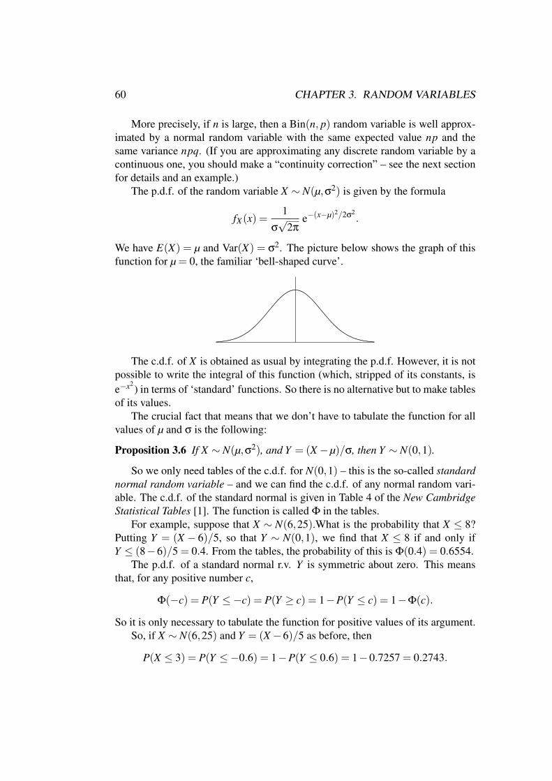
60 CHAPTER 3. RANDOM VARIABLES
More precisely, if n is large, then a Bin(n, p) random variable is well approx-imated by a normal random variable with the same expected value np and thesame variance npq. (If you are approximating any discrete random variable by acontinuous one, you should make a “continuity correction” – see the next sectionfor details and an example.)
The p.d.f. of the random variable X ∼ N(µ,σ2) is given by the formula
fX(x) =1
σ√
2πe−(x−µ)2/2σ2
.
We have E(X) = µ and Var(X) = σ2. The picture below shows the graph of thisfunction for µ = 0, the familiar ‘bell-shaped curve’.
. .................. .................. .......... ......... .......... ......... .......... ...............................
......................
..................................
..............
..........................
..........................
.........................
......................
..................... .......... ......... ......... .......... .......... ........... .......... ............ ...... ........ ...........
........................
..
........................
..
........................
.
............ ........... ........... .............................
....................... ......... .......... ......... .......... .................. ..................
The c.d.f. of X is obtained as usual by integrating the p.d.f. However, it is notpossible to write the integral of this function (which, stripped of its constants, ise−x2
) in terms of ‘standard’ functions. So there is no alternative but to make tablesof its values.
The crucial fact that means that we don’t have to tabulate the function for allvalues of µ and σ is the following:
Proposition 3.6 If X ∼ N(µ,σ2), and Y = (X −µ)/σ, then Y ∼ N(0,1).
So we only need tables of the c.d.f. for N(0,1) – this is the so-called standardnormal random variable – and we can find the c.d.f. of any normal random vari-able. The c.d.f. of the standard normal is given in Table 4 of the New CambridgeStatistical Tables [1]. The function is called Φ in the tables.
For example, suppose that X ∼ N(6,25).What is the probability that X ≤ 8?Putting Y = (X − 6)/5, so that Y ∼ N(0,1), we find that X ≤ 8 if and only ifY ≤ (8−6)/5 = 0.4. From the tables, the probability of this is Φ(0.4) = 0.6554.
The p.d.f. of a standard normal r.v. Y is symmetric about zero. This meansthat, for any positive number c,
Φ(−c) = P(Y ≤−c) = P(Y ≥ c) = 1−P(Y ≤ c) = 1−Φ(c).
So it is only necessary to tabulate the function for positive values of its argument.So, if X ∼ N(6,25) and Y = (X −6)/5 as before, then
P(X ≤ 3) = P(Y ≤−0.6) = 1−P(Y ≤ 0.6) = 1−0.7257 = 0.2743.
3.9. ON USING TABLES 61
3.9 On using tablesWe end this section with a few comments about using tables, not tied particularlyto the normal distribution (though most of the examples will come from there).
InterpolationAny table is limited in the number of entries it contains. Tabulating somethingwith the input given to one extra decimal place would make the table ten times asbulky! Interpolation can be used to extend the range of values tabulated.
Suppose that some function F is tabulated with the input given to three placesof decimals. It is probably true that F is changing at a roughly constant ratebetween, say, 0.28 and 0.29. So F(0.283) will be about three-tenths of the waybetween F(0.28) and F(0.29).
For example, if Φ is the c.d.f. of the normal distribution, then Φ(0.28) =0.6103 and Φ(0.29) = 0.6141, so Φ(0.283) = 0.6114. (Three-tenths of 0.0038 is0.0011.)
Using tables in reverseThis means, if you have a table of values of F , use it to find x such that F(x) is agiven value c. Usually, c won’t be in the table and we have to interpolate betweenvalues x1 and x2, where F(x1) is just less than c and F(x2) is just greater.
For example, if Φ is the c.d.f. of the normal distribution, and we want theupper quartile, then we find from tables Φ(0.67) = 0.7486 and Φ(0.68) = 0.7517,so the required value is about 0.6745 (since 0.0014/0.0031 = 0.45).
In this case, the percentile points of the standard normal r.v. are given in Table5 of the New Cambridge Statistical Tables [1], so you don’t need to do this. Butyou will find it necessary in other cases.
Continuity correctionSuppose we know that a discrete random variable X is well approximated by acontinuous random variable Y . We are given a table of the c.d.f. of Y and want tofind information about X . For example, suppose that X takes integer values andwe want to find P(a ≤ X ≤ b), where a and b are integers. This probability isequal to
P(X = a)+P(x = a+1)+ · · ·+P(X = b).
To say that X can be approximated by Y means that, for example, P(X = a) isapproximately equal to fY (a), where fY is the p.d.f. of Y . This is equal to the area
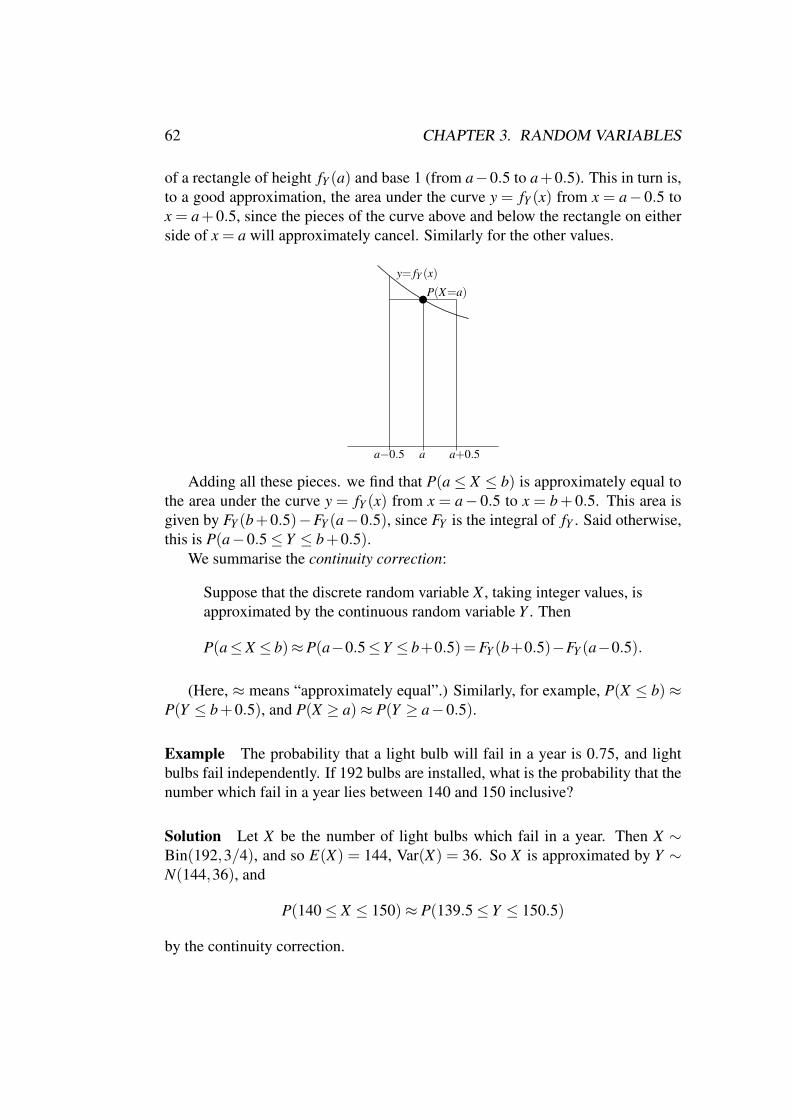
62 CHAPTER 3. RANDOM VARIABLES
of a rectangle of height fY (a) and base 1 (from a−0.5 to a+0.5). This in turn is,to a good approximation, the area under the curve y = fY (x) from x = a− 0.5 tox = a+0.5, since the pieces of the curve above and below the rectangle on eitherside of x = a will approximately cancel. Similarly for the other values.
...............
...................
..............................
..
................................
...............................
..............................
.............................
.............................
............................
y= fY (x)uP(X=a)
a−0.5 a a+0.5
Adding all these pieces. we find that P(a ≤ X ≤ b) is approximately equal tothe area under the curve y = fY (x) from x = a− 0.5 to x = b + 0.5. This area isgiven by FY (b+0.5)−FY (a−0.5), since FY is the integral of fY . Said otherwise,this is P(a−0.5 ≤ Y ≤ b+0.5).
We summarise the continuity correction:
Suppose that the discrete random variable X , taking integer values, isapproximated by the continuous random variable Y . Then
P(a≤X ≤ b)≈P(a−0.5≤Y ≤ b+0.5) = FY (b+0.5)−FY (a−0.5).
(Here, ≈ means “approximately equal”.) Similarly, for example, P(X ≤ b)≈P(Y ≤ b+0.5), and P(X ≥ a)≈ P(Y ≥ a−0.5).
Example The probability that a light bulb will fail in a year is 0.75, and lightbulbs fail independently. If 192 bulbs are installed, what is the probability that thenumber which fail in a year lies between 140 and 150 inclusive?
Solution Let X be the number of light bulbs which fail in a year. Then X ∼Bin(192,3/4), and so E(X) = 144, Var(X) = 36. So X is approximated by Y ∼N(144,36), and
P(140 ≤ X ≤ 150)≈ P(139.5 ≤ Y ≤ 150.5)
by the continuity correction.
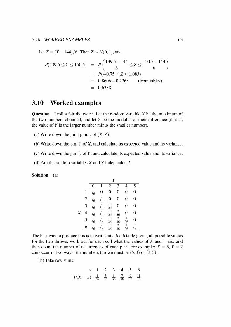
3.10. WORKED EXAMPLES 63
Let Z = (Y −144)/6. Then Z ∼ N(0,1), and
P(139.5 ≤ Y ≤ 150.5) = P(
139.5−1446
≤ Z ≤ 150.5−1446
)= P(−0.75 ≤ Z ≤ 1.083)= 0.8606−0.2268 (from tables)= 0.6338.
3.10 Worked examplesQuestion I roll a fair die twice. Let the random variable X be the maximum ofthe two numbers obtained, and let Y be the modulus of their difference (that is,the value of Y is the larger number minus the smaller number).
(a) Write down the joint p.m.f. of (X ,Y ).
(b) Write down the p.m.f. of X , and calculate its expected value and its variance.
(c) Write down the p.m.f. of Y , and calculate its expected value and its variance.
(d) Are the random variables X and Y independent?
Solution (a)Y
0 1 2 3 4 51 1
36 0 0 0 0 0
2 136
236 0 0 0 0
3 136
236
236 0 0 0
X 4 136
236
236
236 0 0
5 136
236
236
236
236 0
6 136
236
236
236
236
236
The best way to produce this is to write out a 6×6 table giving all possible valuesfor the two throws, work out for each cell what the values of X and Y are, andthen count the number of occurrences of each pair. For example: X = 5, Y = 2can occur in two ways: the numbers thrown must be (5,3) or (3,5).
(b) Take row sums:
x 1 2 3 4 5 6
P(X = x) 136
336
536
736
936
1136
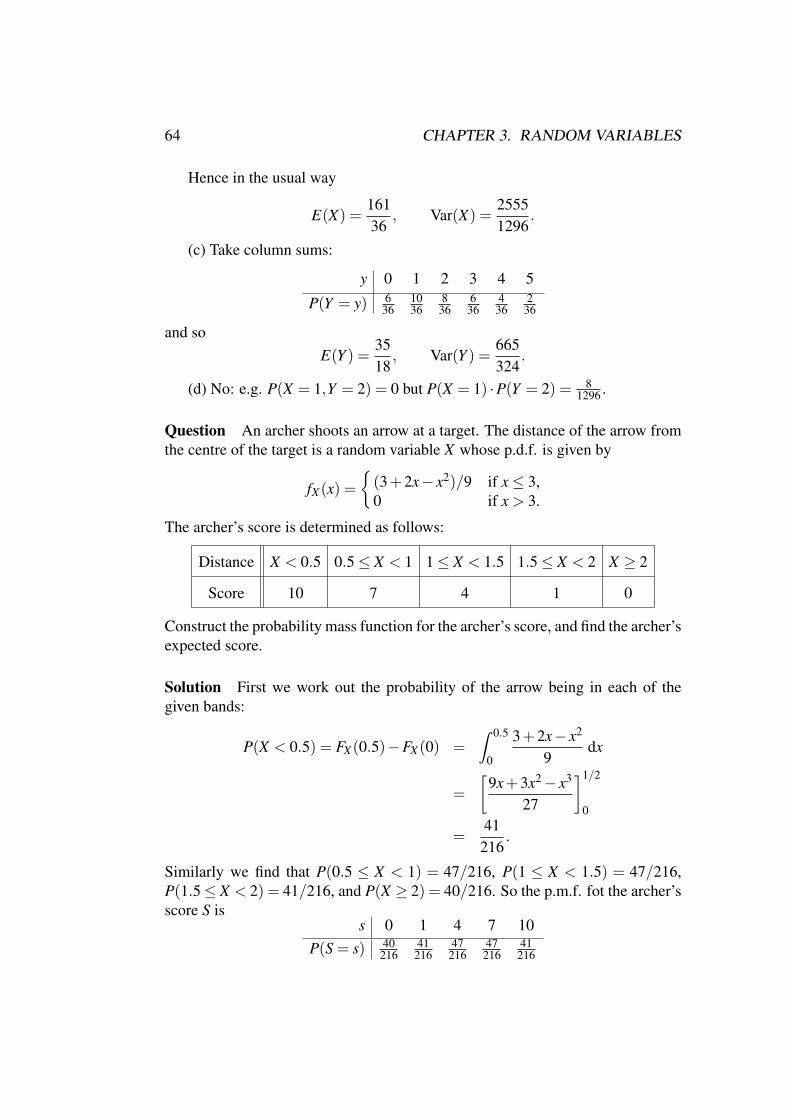
64 CHAPTER 3. RANDOM VARIABLES
Hence in the usual way
E(X) =16136
, Var(X) =25551296
.
(c) Take column sums:
y 0 1 2 3 4 5
P(Y = y) 636
1036
836
636
436
236
and soE(Y ) =
3518
, Var(Y ) =665324
.
(d) No: e.g. P(X = 1,Y = 2) = 0 but P(X = 1) ·P(Y = 2) = 81296 .
Question An archer shoots an arrow at a target. The distance of the arrow fromthe centre of the target is a random variable X whose p.d.f. is given by
fX(x) =
(3+2x− x2)/9 if x ≤ 3,0 if x > 3.
The archer’s score is determined as follows:
Distance X < 0.5 0.5 ≤ X < 1 1 ≤ X < 1.5 1.5 ≤ X < 2 X ≥ 2
Score 10 7 4 1 0
Construct the probability mass function for the archer’s score, and find the archer’sexpected score.
Solution First we work out the probability of the arrow being in each of thegiven bands:
P(X < 0.5) = FX(0.5)−FX(0) =Z 0.5
0
3+2x− x2
9dx
=[
9x+3x2− x3
27
]1/2
0
=41
216.
Similarly we find that P(0.5 ≤ X < 1) = 47/216, P(1 ≤ X < 1.5) = 47/216,P(1.5≤ X < 2) = 41/216, and P(X ≥ 2) = 40/216. So the p.m.f. fot the archer’sscore S is
s 0 1 4 7 10P(S = s) 40
21641216
47216
47216
41216
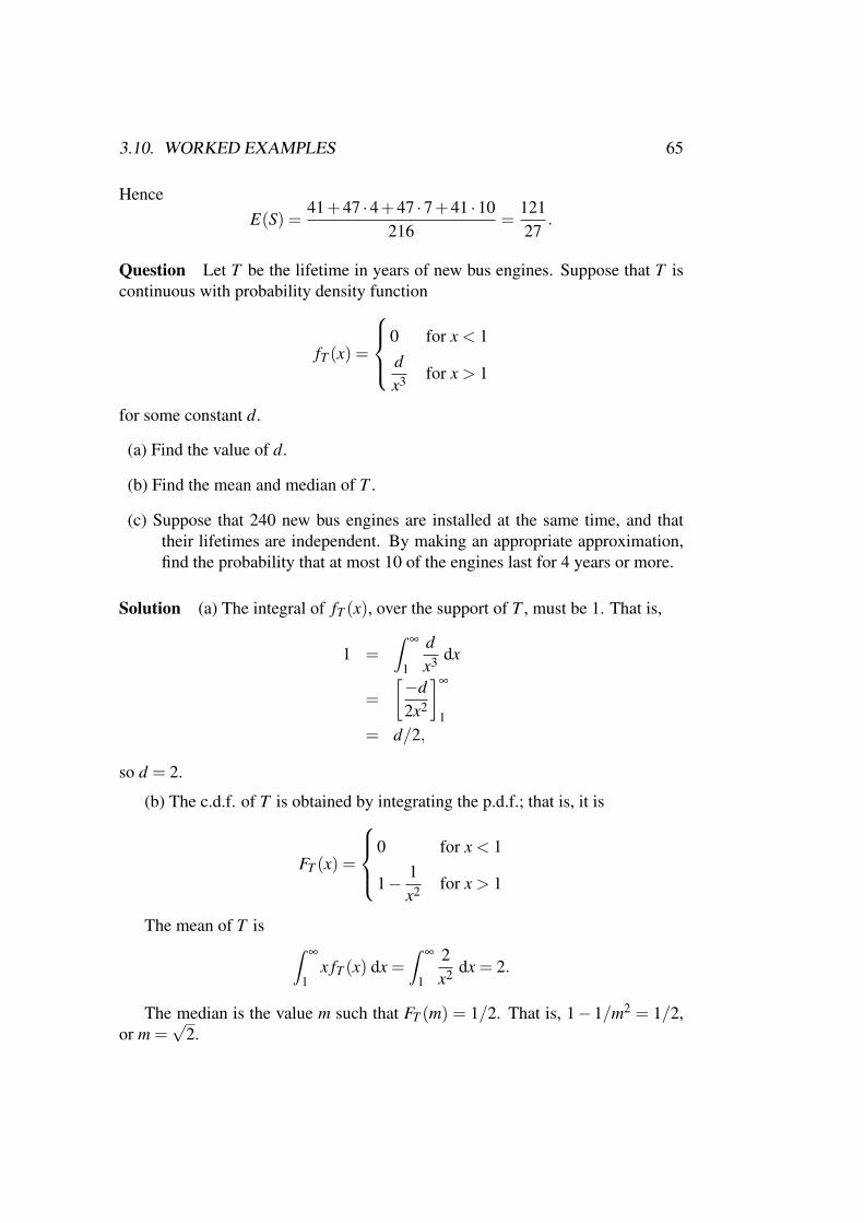
3.10. WORKED EXAMPLES 65
HenceE(S) =
41+47 ·4+47 ·7+41 ·10216
=12127
.
Question Let T be the lifetime in years of new bus engines. Suppose that T iscontinuous with probability density function
fT (x) =
0 for x < 1dx3 for x > 1
for some constant d.
(a) Find the value of d.
(b) Find the mean and median of T .
(c) Suppose that 240 new bus engines are installed at the same time, and thattheir lifetimes are independent. By making an appropriate approximation,find the probability that at most 10 of the engines last for 4 years or more.
Solution (a) The integral of fT (x), over the support of T , must be 1. That is,
1 =Z
∞
1
dx3 dx
=[−d2x2
]∞
1= d/2,
so d = 2.
(b) The c.d.f. of T is obtained by integrating the p.d.f.; that is, it is
FT (x) =
0 for x < 1
1− 1x2 for x > 1
The mean of T is Z∞
1x fT (x) dx =
Z∞
1
2x2 dx = 2.
The median is the value m such that FT (m) = 1/2. That is, 1− 1/m2 = 1/2,or m =
√2.
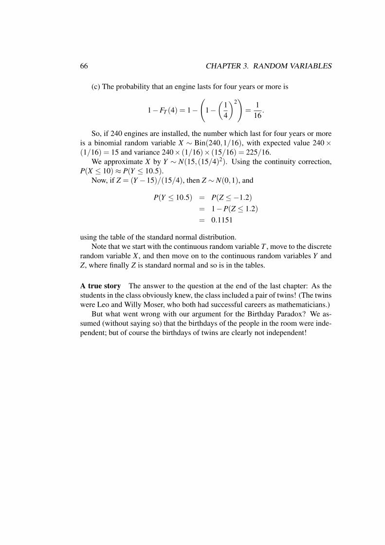
66 CHAPTER 3. RANDOM VARIABLES
(c) The probability that an engine lasts for four years or more is
1−FT (4) = 1−
(1−(
14
)2)
=1
16.
So, if 240 engines are installed, the number which last for four years or moreis a binomial random variable X ∼ Bin(240,1/16), with expected value 240×(1/16) = 15 and variance 240× (1/16)× (15/16) = 225/16.
We approximate X by Y ∼ N(15,(15/4)2). Using the continuity correction,P(X ≤ 10)≈ P(Y ≤ 10.5).
Now, if Z = (Y −15)/(15/4), then Z ∼ N(0,1), and
P(Y ≤ 10.5) = P(Z ≤−1.2)= 1−P(Z ≤ 1.2)= 0.1151
using the table of the standard normal distribution.Note that we start with the continuous random variable T , move to the discrete
random variable X , and then move on to the continuous random variables Y andZ, where finally Z is standard normal and so is in the tables.
A true story The answer to the question at the end of the last chapter: As thestudents in the class obviously knew, the class included a pair of twins! (The twinswere Leo and Willy Moser, who both had successful careers as mathematicians.)
But what went wrong with our argument for the Birthday Paradox? We as-sumed (without saying so) that the birthdays of the people in the room were inde-pendent; but of course the birthdays of twins are clearly not independent!
Chapter 4
More on joint distribution
We have seen the joint p.m.f. of two discrete random variables X and Y , and wehave learned what it means for X and Y to be independent. Now we examinethis further to see measures of non-independence and conditional distributions ofrandom variables.
4.1 Covariance and correlationIn this section we consider a pair of discrete random variables X and Y . Rememberthat X and Y are independent if
P(X = ai,Y = b j) = P(X = ai) ·P(Y = b j)
holds for any pair (ai,b j) of values of X and Y . We introduce a number (calledthe covariance of X and Y ) which gives a measure of how far they are from beingindependent.
Look back at the proof of Theorem 21(b), where we showed that if X and Yare independent then Var(X +Y ) = Var(X)+Var(Y ). We found that, in any case,
Var(X +Y ) = Var(X)+Var(Y )+2(E(XY )−E(X)E(Y )),
and then proved that if X and Y are independent then E(XY ) = E(X)E(Y ), so thatthe last term is zero.
Now we define the covariance of X and Y to be E(XY )−E(X)E(Y ). Wewrite Cov(X ,Y ) for this quantity. Then the argument we had earlier shows thefollowing:
Theorem 4.1 (a) Var(X +Y ) = Var(X)+Var(Y )+2Cov(X ,Y ).
(b) If X and Y are independent, then Cov(X ,Y ) = 0.
67
68 CHAPTER 4. MORE ON JOINT DISTRIBUTION
In fact, a more general version of (a), proved by the same argument, says that
Var(aX +bY ) = a2 Var(X)+b2 Var(Y )+2abCov(X ,Y ). (4.1)
Another quantity closely related to covariance is the correlation coefficient,corr(X ,Y ), which is just a “normalised” version of the covariance. It is defined asfollows:
corr(X ,Y ) =Cov(X ,Y )√
Var(X)Var(Y ).
The point of this is the first part of the following theorem.
Theorem 4.2 Let X and Y be random variables. Then
(a) −1 ≤ corr(X ,Y )≤ 1;
(b) if X and Y are independent, then corr(X ,Y ) = 0;
(c) if Y = mX + c for some constants m 6= 0 and c, then corr(X ,Y ) = 1 if m > 0,and corr(X ,Y ) =−1 if m < 0.
The proof of the first part is optional: see the end of this section. But note thatthis is another check on your calculations: if you calculate a correlation coefficientwhich is bigger than 1 or smaller than −1, then you have made a mistake. Part (b)follows immediately from part (b) of the preceding theorem.
For part (c), suppose that Y = mX +c. Let E(X) = µ and Var(X) = α, so that E(X2) = µ2 +α.Now we just calculate everything in sight.
E(Y ) = E(mX + c) = mE(X)+ c = mµ+ c
E(Y 2) = E(m2X2 +2mcX + c2) = m2(µ2 +α)+2mcµ+ c2
Var(Y ) = E(Y 2)−E(Y )2 = m2α
E(XY ) = E(mX2 + cX) = m(µ2 +α)+ cµ;
Cov(X ,Y ) = E(XY )−E(X)E(Y ) = mα
corr(X ,Y ) = Cov(X ,Y )/√
Var(X)Var(Y ) = mα/√
m2α2
=+1 if m > 0,−1 if m < 0.
Thus the correlation coefficient is a measure of the extent to which the twovariables are related. It is +1 if Y increases linearly with X ; 0 if there is no relationbetween them; and −1 if Y decreases linearly as X increases. More generally, apositive correlation indicates a tendency for larger X values to be associated withlarger Y values; a negative value, for smaller X values to be associated with largerY values.
4.1. COVARIANCE AND CORRELATION 69
Example I have two red pens, one green pen, and one blue pen, and I choosetwo pens without replacement. Let X be the number of red pens that I choose andY the number of green pens. Then the joint p.m.f. of X and Y is given by thefollowing table:
Y0 1
0 0 16
X 1 13
13
2 16 0
From this we can calculate the marginal p.m.f. of X and of Y and hence findtheir expected values and variances:
E(X) = 1, Var(X) = 1/3,
E(Y ) = 1/2, Var(Y ) = 1/4.
Also, E(XY ) = 1/3, since the sum
E(XY ) = ∑i, j
aib jP(X = ai,Y = b j)
contains only one term where all three factors are non-zero. Hence
Cov(X ,Y ) = 1/3−1/2 =−1/6,
and
corr(X ,Y ) =−1/6√
1/12=− 1√
3.
The negative correlation means that small values of X tend to be associated withlarger values of Y . Indeed, if X = 0 then Y must be 1, and if X = 2 then Y mustbe 0, but if X = 1 then Y can be either 0 or 1.
Example We have seen that if X and Y are independent then Cov(X ,Y ) = 0.However, it doesn’t work the other way around. Consider the following jointp.m.f.
Y−1 0 1
−1 15 0 1
5
X 0 0 15 0
1 15 0 1
5
70 CHAPTER 4. MORE ON JOINT DISTRIBUTION
Now calculation shows that E(X) = E(Y ) = E(XY ) = 0, so Cov(X ,Y ) = 0. ButX and Y are not independent: for P(X =−1) = 2/5, P(Y = 0) = 1/5, but P(X =−1,Y = 0) = 0.
We call two random variables X and Y uncorrelated if Cov(X ,Y ) = 0 (in otherwords, if corr(X ,Y ) = 0). So we can say:
Independent random variables are uncorrelated, but uncorrelated ran-dom variables need not be independent.
Here is the proof that the correlation coefficient lies between −1 and 1. Clearly this is exactlyequivalent to proving that its square is at most 1, that is, that
Cov(X ,Y )2 ≤ Var(X) ·Var(Y ).
This depends on the following fact:
Let p,q,r be real numbers with p > 0. Suppose that px2 + 2qx + r ≥ 0 for all realnumbers x. Then q2 ≤ pr.
For, when we plot the graph y = px2 + 2qx + r, we get a parabola; the hypothesis means that thisparabola never goes below the X-axis, so that either it lies entirely above the axis, or it touches itin one point. This means that the quadratic equation px2 +2qx+ r = 0 either has no real roots, orhas two equal real roots. From high-school algebra, we know that this means that q2 ≤ pr.
Now let p = Var(X), q = Cov(X ,Y ), and r = Var(Y ). Equation (4.1) shows that
px2 +2qx+ r = Var(xX +Y ).
(Note that x is an arbitrary real number here and has no connection with the random variable X!)Since the variance of a random variable is never negative, we see that px2 +2qx+r ≥ 0 for all
choices of x. Now our argument above shows that q2 ≤ pr, that is, Cov(X ,Y )2 ≤ Var(X) ·Var(Y ),as required.
4.2 Conditional random variablesRemember that the conditional probability of event B given event A is P(B | A) =P(A∩B)/P(A).
Suppose that X is a discrete random variable. Then the conditional probabilitythat X takes a certain value ai, given A, is just
P(X = ai | A) =P(A holds and X = ai)
P(A).
This defines the probability mass function of the conditional random variableX | A.
So we can, for example, talk about the conditional expectation
E(X | A) = ∑i
aiP(X = ai | A).
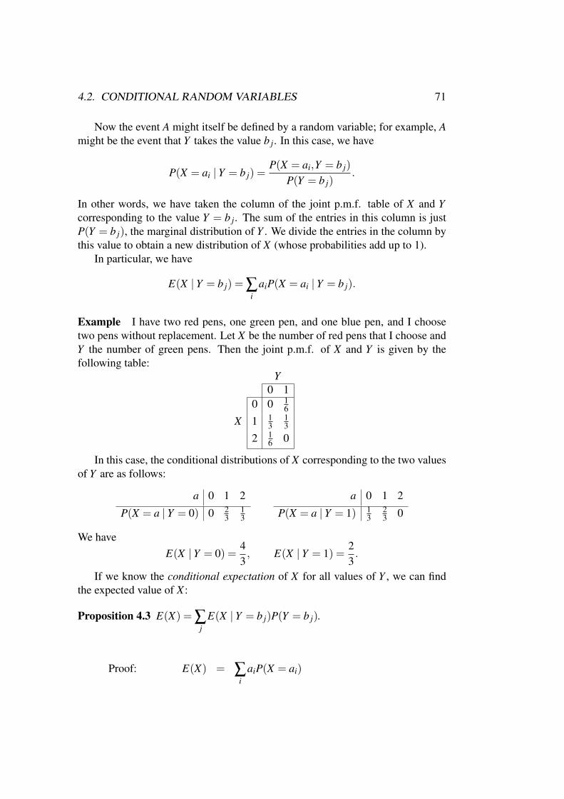
4.2. CONDITIONAL RANDOM VARIABLES 71
Now the event A might itself be defined by a random variable; for example, Amight be the event that Y takes the value b j. In this case, we have
P(X = ai | Y = b j) =P(X = ai,Y = b j)
P(Y = b j).
In other words, we have taken the column of the joint p.m.f. table of X and Ycorresponding to the value Y = b j. The sum of the entries in this column is justP(Y = b j), the marginal distribution of Y . We divide the entries in the column bythis value to obtain a new distribution of X (whose probabilities add up to 1).
In particular, we have
E(X | Y = b j) = ∑i
aiP(X = ai | Y = b j).
Example I have two red pens, one green pen, and one blue pen, and I choosetwo pens without replacement. Let X be the number of red pens that I choose andY the number of green pens. Then the joint p.m.f. of X and Y is given by thefollowing table:
Y0 1
0 0 16
X 1 13
13
2 16 0
In this case, the conditional distributions of X corresponding to the two valuesof Y are as follows:
a 0 1 2
P(X = a | Y = 0) 0 23
13
a 0 1 2
P(X = a | Y = 1) 13
23 0
We haveE(X | Y = 0) =
43, E(X | Y = 1) =
23.
If we know the conditional expectation of X for all values of Y , we can findthe expected value of X :
Proposition 4.3 E(X) = ∑j
E(X | Y = b j)P(Y = b j).
Proof: E(X) = ∑i
aiP(X = ai)
72 CHAPTER 4. MORE ON JOINT DISTRIBUTION
= ∑i
ai ∑j
P(X = ai | Y = b j)P(Y = b j)
= ∑j
(∑
iaiP(X = ai | Y = b j
)P(Y = b j)
= ∑j
E(X | Y = b j)P(Y = b j).
In the above example, we have
E(X) = E(X | Y = 0)P(Y = 0)+E(X | Y = 1)P(Y = 1)= (4/3)× (1/2)+(2/3)× (1/2)= 1.
Example Let us revisit the geometric random variable and calculate its expectedvalue. Recall the situation: I have a coin with probability p of showing heads; Itoss it repeatedly until heads appears for the first time; X is the number of tosses.
Let Y be the Bernoulli random variable whose value is 1 if the result of thefirst toss is heads, 0 if it is tails. If Y = 1, then we stop the experiment then andthere; so if Y = 1, then necessarily X = 1, and we have E(X | Y = 1) = 1. Onthe other hand, if Y = 0, then the sequence of tosses from that point on has thesame distribution as the original experiment; so E(X | Y = 0) = 1 + E(X) (the 1counting the first toss). So
E(X) = E(X | Y = 0)P(Y = 0)+E(X | Y = 1)P(Y = 1)= (1+E(X)) ·q+1 · p= E(X)(1− p)+1;
rearranging this equation, we find that E(X) = 1/p, confirming our earlier value.
In Proposition 2.1, we saw that independence of events can be characterisedin terms of conditional probabilities: A and B are independent if and only if theysatisfy P(A | B) = P(A). A similar result holds for independence of random vari-ables:
Proposition 4.4 Let X and Y be discrete random variables. Then X and Y areindependent if and only if, for any values ai and b j of X and Y respectively, wehave
P(X = ai | Y = b j) = P(X = ai).
This is obtained by applying Proposition 15 to the events X = ai and Y = b j.It can be stated in the following way: X and Y are independent if the conditionalp.m.f. of X | (Y = b j) is equal to the p.m.f. of X , for any value b j of Y .
4.3. JOINT DISTRIBUTION OF CONTINUOUS R.V.S 73
4.3 Joint distribution of continuous r.v.sFor continuous random variables, the covariance and correlation can be definedby the same formulae as in the discrete case; and Equation (4.1) remains valid.But we have to examine what is meant by independence for continuous randomvariables. The formalism here needs even more concepts from calculus than wehave used before: functions of two variables, partial derivatives, double integrals.I assume that this is unfamiliar to you, so this section will be brief and can mostlybe skipped.
Let X and Y be continuous random variables. The joint cumulative distributionfunction of X and Y is the function FX ,Y of two real variables given by
FX ,Y (x,y) = P(X ≤ x,Y ≤ y).
We define X and Y to be independent if P(X ≤ x,Y ≤ y) = P(X ≤ x) ·P(Y ≤ y),for any x and y, that is, FX ,Y (x,y) = FX(x) ·FY (y). (Note that, just as in the one-variable case, X is part of the name of the function, while x is the argument of thefunction.)
The joint probability density function of X and Y is
fX ,Y (x,y) =∂2
∂x∂yFX ,Y (x,y).
In other words, differentiate with respect to x keeping y constant, and then differ-entiate with respect to y keeping x constant (or the other way round: the answer isthe same for all functions we consider.)
The probability that the pair of values of (X ,Y ) corresponds to a point in someregion of the plane is obtained by taking the double integral of fX ,Y over thatregion. For example,
P(a ≤ X ≤ b,c ≤ Y ≤ d) =Z d
c
Z b
afX ,Y (x,y)dx dy
(the right hand side means, integrate with respect to x between a and b keeping yfixed; the result is a function of y; integrate this function with respect to y from cto d.)
The marginal p.d.f. of X is given by
fX(x) =Z
∞
−∞
fX ,Y (x,y)dy,
and the marginal p.d.f. of Y is similarly
fY (y) =Z
∞
−∞
fX ,Y (x,y)dx.
74 CHAPTER 4. MORE ON JOINT DISTRIBUTION
Then the conditional p.d.f. of X | (Y = b) is
fX |(Y=b)(x) =fX ,Y (x,b)
fY (b).
The expected value of XY is, not surprisingly,
E(XY ) =Z
∞
−∞
Z∞
−∞
xy fX ,Y (x,y)dx dy,
and then as in the discrete case
Cov(X ,Y ) = E(XY )−E(X)E(Y ), corr(X ,Y ) =Cov(X ,Y )√
Var(X)Var(Y ).
Finally, and importantly,
The continuous random variables X and Y are independent if and onlyif
fX ,Y (x,y) = fX(x) · fY (y).
As usual this holds if and only if the conditional p.d.f. of X | (Y = b) is equal tothe marginal p.d.f. of X , for any value b. Also, if X and Y are independent, thenCov(X ,Y ) = corr(X ,Y ) = 0 (but not conversely!).
4.4 Transformation of random variablesIf a continuous random variable Y is a function of another r.v. X , we can find thedistribution of Y in terms of that of X .
Example Let X and Y be random variables. Suppose that X ∼U [0,4] (uniformon [0,4]) and Y =
√X . What is the support of Y ? Find the cumulative distribution
function and the probability density function of Y .
Solution (a) The support of X is [0,4], and Y =√
X , so the support of Y is [0,2].(b) We have fX(x) = x/4 for 0 ≤ x ≤ 4. Now
FY (y) = P(Y ≤ y)= P(X ≤ y2)= FX(y2)= y2/4
4.4. TRANSFORMATION OF RANDOM VARIABLES 75
for 0 ≤ y ≤ 2; of course FY (y) = 0 for y < 0 and FY (y) = 1 for y > 2. (Note thatY ≤ y if and only if X ≤ y2, since Y =
√X .)
(c) We have
fY (y) =ddy
FY (y) =
y/2 if 0 ≤ y ≤ 2,0 otherwise.
The argument in (b) is the key. If we know Y as a function of X , say Y = g(X),where g is an increasing function, then the event Y ≤ y is the same as the eventX ≤ h(Y ), where h is the inverse function of g. This means that y = g(x) if andonly if x = h(y). (In our example, g(x) =
√x, and so h(y) = y2.) Thus
FY (y) = FX(h(y)),
and so, by the Chain Rule,
fY (y) = fX(h(y))h′(y),
where h′ is the derivative of h. (This is because fX(x) is the derivative of FX(x)with respect to its argument x, and the Chain Rule says that if x = h(y) we mustmultiply by h′(y) to find the derivative with respect to y.)
Applying this formula in our example we have
fY (y) =14·2y =
y2
for 0 ≤ y ≤ 2, since the p.d.f. of X is fX(x) = 1/4 for 0 ≤ x ≤ 4.Here is a formal statement of the result.
Theorem 4.5 Let X be a continuous random variable. Let g be a real functionwhich is either strictly increasing or strictly decreasing on the support of X, andwhich is differentiable there. Let Y = g(X). Then
(a) the support of Y is the image of the support of X under g;
(b) the p.d.f. of Y is given by fY (y) = fX(h(y))|h′(y)|, where h is the inversefunction of g.
For example, here is the proof of Proposition 3.6: if X ∼ N(µ,σ2) and Y =(X −µ)/σ, then Y ∼ N(0,1). Recall that
fX(x) =1
σ√
2πe−(x−µ)2/2σ2
.
76 CHAPTER 4. MORE ON JOINT DISTRIBUTION
We have Y = g(X), where g(x) = (x− µ)/σ; this function is everywhere strictlyincreasing (the graph is a straight line with slope 1/σ), and the inverse function isx = h(y) = σy+µ. Thus, h′(y) = σ, and
fY (y) = fX(σy+µ) ·σ =1√2π
e−y2/2,
the p.d.f. of a standard normal variable.
However, rather than remember this formula, together with the conditions forits validity, I recommend going back to the argument we used in the example.
If the transforming function g is not monotonic (that is, not either increasingor decreasing), then life is a bit more complicated. For example, if X is a randomvariable taking both positive and negative values, and Y = X2, then a given valuey of Y could arise from either of the values
√y and −
√y of X , so we must work
out the two contributions and add them up.
Example X ∼ N(0,1) and Y = X2. Find the p.d.f. of Y .
The p.d.f. of X is (1/√
2π)e−x2/2. Let Φ(x) be its c.d.f., so that P(X ≤ x) =Φ(x), and
Φ′(x) =
1√2π
e−x2/2.
Now Y = X2, so Y ≤ y if and only if −√
y ≤ X ≤√
y. Thus
FY (y) = P(Y ≤ y)
= P(−√
y ≤ X ≤√
y)
= Φ(√
y)−Φ(−√
y)
= Φ(√
y− (1−Φ(√
y)) (by symmetry of N(0,1))
= 2Φ(√
y)−1.
So
fY (y) =ddy
FY (y)
= 2Φ′(√
y) · 12√
y(by the Chain Rule)
=1√2πy
e−y/2.
Of course, this is valid for y > 0; for y < 0, the p.d.f. is zero.
4.5. WORKED EXAMPLES 77
Note the 2 in the line labelled “by the Chain Rule”. If you blindly appliedthe formula of Theorem 4.5, using h(y) =
√y, you would not get this 2; it arises
from the fact that, since Y = X2, each value of Y corresponds to two values of X(one positive, one negative), and each value gives the same contribution, by thesymmetry of the p.d.f. of X .
4.5 Worked examplesQuestion Two numbers X and Y are chosen independently from the uniformdistribution on the unit interval [0,1]. Let Z be the maximum of the two numbers.Find the p.d.f. of Z, and hence find its expected value, variance and median.
Solution The c.d.f.s of X and Y are identical, that is,
FX(x) = FY (x) =
0 if x < 0,x if 0 < x < 1,1 if x > 1.
(The variable can be called x in both cases; its name doesn’t matter.)The key to the argument is to notice that
Z = max(X ,Y )≤ x if and only if X ≤ x and Y ≤ x.
(For, if both X and Y are smaller than a given value x, then so is their maximum;but if at least one of them is greater than x, then again so is their maximum.) For0 ≤ x ≤ 1, we have P(X ≤ x) = P(Y ≤ x) = x; by independence,
P(X ≤ x and Y ≤ x) = x · x = x2.
Thus P(Z ≤ x) = x2. Of course this probability is 0 if x < 0 and is 1 if x > 1. Sothe c.d.f. of Z is
FZ(x) =
0 if x < 0,x2 if 0 < x < 1,1 if x > 1.
The median of Z is the value of m such that FZ(m) = 1/2, that is m2 = 1/2, orm = 1/
√2.
We obtain the p.d.f. of Z by differentiating:
fZ(x) =2x if 0 < x < 1,
0 otherwise.
Then we can find E(Z) and Var(Z) in the usual way:
E(Z) =Z 1
02x2dx =
23, Var(Z) =
Z 1
02x3dx−
(23
)2
=118
.
78 CHAPTER 4. MORE ON JOINT DISTRIBUTION
Question I roll a fair die bearing the numbers 1 to 6. If N is the number showingon the die, I then toss a fair coin N times. Let X be the number of heads I obtain.
(a) Write down the p.m.f. for X .
(b) Calculate E(X) without using this information.
Solution (a) If we were given that N = n, say, then X would be a binomialBin(n,1/2) random variable. So P(X = k | N = n) = nCk(1/2)n.
By the ToTP,
P(X = k) =6
∑n=1
P(X = k | N = n)P(N = n).
Clearly P(N = n) = 1/6 for n = 1, . . . ,6. So to find P(X = k), we add up theprobability that X = k for a Bin(n,1/2) r.v. for n = k, . . . ,6 and divide by 6. (Westart at k because you can’t get k heads with fewer than k coin tosses!) The answercomes to
k 0 1 2 3 4 5 6P(X = k) 63
384120384
99384
64384
29384
8384
1384
For example,
P(X = 4) =4C4(1/2)4 + 5C4(1/2)5 + 6C4(1/2)6
6=
4+10+15384
.
(b) By Proposition 4.3,
E(X) =6
∑n=1
E(X | (N = n))P(N = n).
Now if we are given that N = n then, as we remarked, X has a binomial Bin(n,1/2)distribution, with expected value n/2. So
E(X) =6
∑n=1
(n/2) · (1/6) =1+2+3+4+5+6
2 ·6=
74.
Try working it out from the p.m.f. to check that the answer is the same!
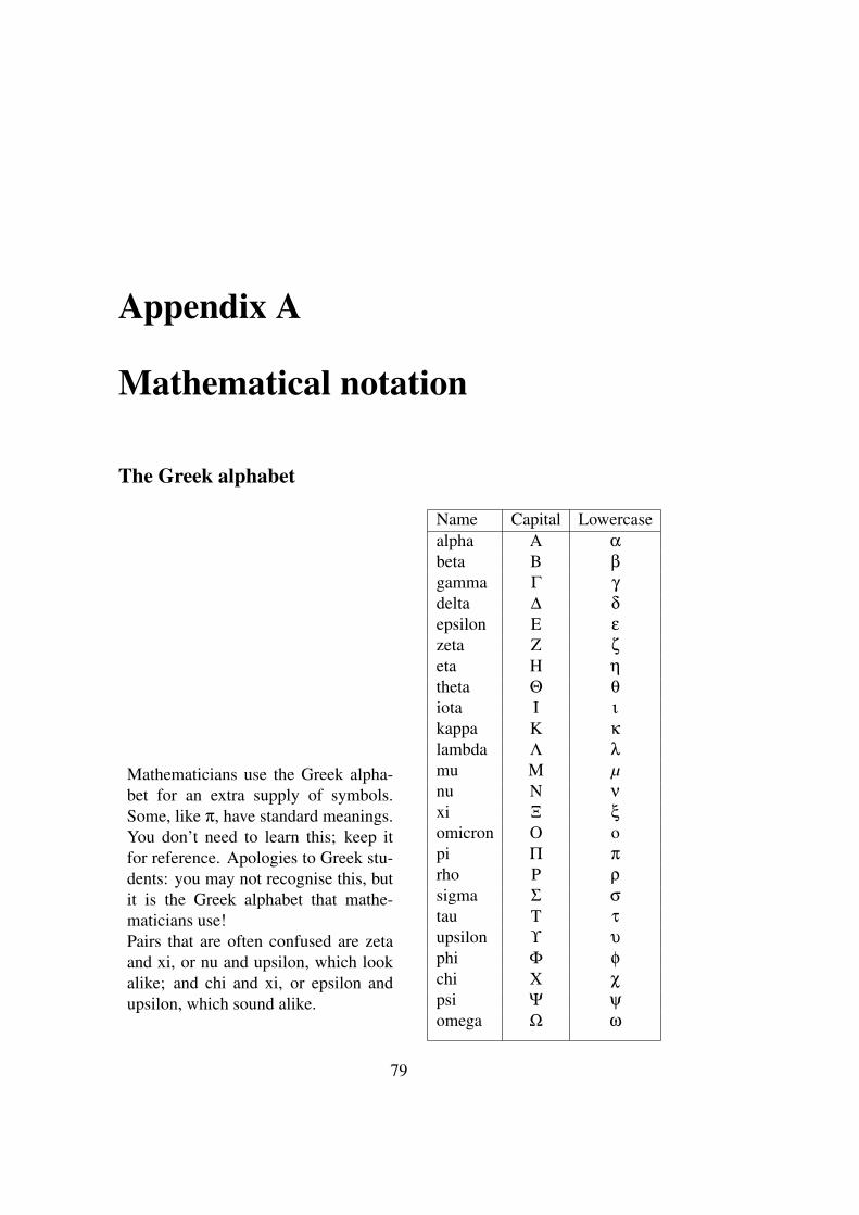
Appendix A
Mathematical notation
The Greek alphabet
Mathematicians use the Greek alpha-bet for an extra supply of symbols.Some, like π, have standard meanings.You don’t need to learn this; keep itfor reference. Apologies to Greek stu-dents: you may not recognise this, butit is the Greek alphabet that mathe-maticians use!Pairs that are often confused are zetaand xi, or nu and upsilon, which lookalike; and chi and xi, or epsilon andupsilon, which sound alike.
Name Capital Lowercasealpha A α
beta B β
gamma Γ γ
delta ∆ δ
epsilon E ε
zeta Z ζ
eta H η
theta Θ θ
iota I ι
kappa K κ
lambda Λ λ
mu M µnu N ν
xi Ξ ξ
omicron O opi Π π
rho P ρ
sigma Σ σ
tau T τ
upsilon ϒ υ
phi Φ φ
chi X χ
psi Ψ ψ
omega Ω ω
79
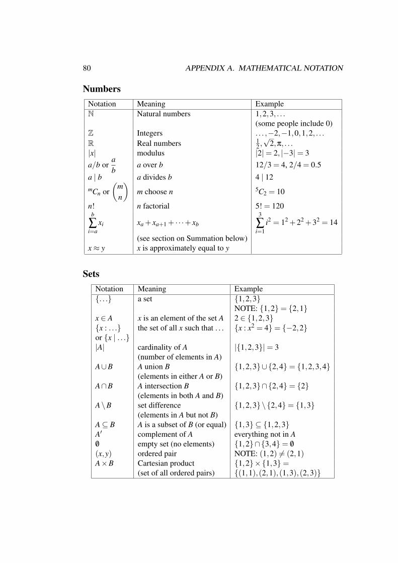
80 APPENDIX A. MATHEMATICAL NOTATION
NumbersNotation Meaning ExampleN Natural numbers 1,2,3, . . .
(some people include 0)Z Integers . . . ,−2,−1,0,1,2, . . .
R Real numbers 12 ,√
2,π, . . .|x| modulus |2|= 2, |−3|= 3a/b or
ab
a over b 12/3 = 4, 2/4 = 0.5
a | b a divides b 4 | 12mCn or
(mn
)m choose n 5C2 = 10
n! n factorial 5! = 120b
∑i=a
xi xa + xa+1 + · · ·+ xb
3
∑i=1
i2 = 12 +22 +32 = 14
(see section on Summation below)x ≈ y x is approximately equal to y
SetsNotation Meaning Example. . . a set 1,2,3
NOTE: 1,2= 2,1x ∈ A x is an element of the set A 2 ∈ 1,2,3x : . . . the set of all x such that . . . x : x2 = 4= −2,2or x | . . .|A| cardinality of A |1,2,3|= 3
(number of elements in A)A∪B A union B 1,2,3∪2,4= 1,2,3,4
(elements in either A or B)A∩B A intersection B 1,2,3∩2,4= 2
(elements in both A and B)A\B set difference 1,2,3\2,4= 1,3
(elements in A but not B)A ⊆ B A is a subset of B (or equal) 1,3 ⊆ 1,2,3A′ complement of A everything not in A/0 empty set (no elements) 1,2∩3,4= /0
(x,y) ordered pair NOTE: (1,2) 6= (2,1)A×B Cartesian product 1,2×1,3=
(set of all ordered pairs) (1,1),(2,1),(1,3),(2,3)
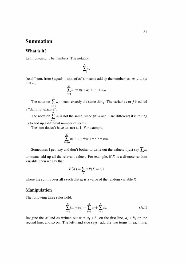
81
Summation
What is it?Let a1,a2,a3, . . . be numbers. The notation
n
∑i=1
ai
(read “sum, from i equals 1 to n, of ai”), means: add up the numbers a1,a2, . . . ,an;that is,
n
∑i=1
ai = a1 +a2 + · · ·+an.
The notationn
∑j=1
a j means exactly the same thing. The variable i or j is called
a “dummy variable”.
The notationm
∑i=1
ai is not the same, since (if m and n are different) it is telling
us to add up a different number of terms.The sum doesn’t have to start at 1. For example,
20
∑i=10
ai = a10 +a11 + · · ·+a20.
Sometimes I get lazy and don’t bother to write out the values: I just say ∑i
ai
to mean: add up all the relevant values. For example, if X is a discrete randomvariable, then we say that
E(X) = ∑i
aiP(X = ai)
where the sum is over all i such that ai is a value of the random variable X .
ManipulationThe following three rules hold.
n
∑i=1
(ai +bi) =n
∑i=1
ai +n
∑i=1
bi. (A.1)
Imagine the as and bs written out with a1 + b1 on the first line, a2 + b2 on thesecond line, and so on. The left-hand side says: add the two terms in each line,
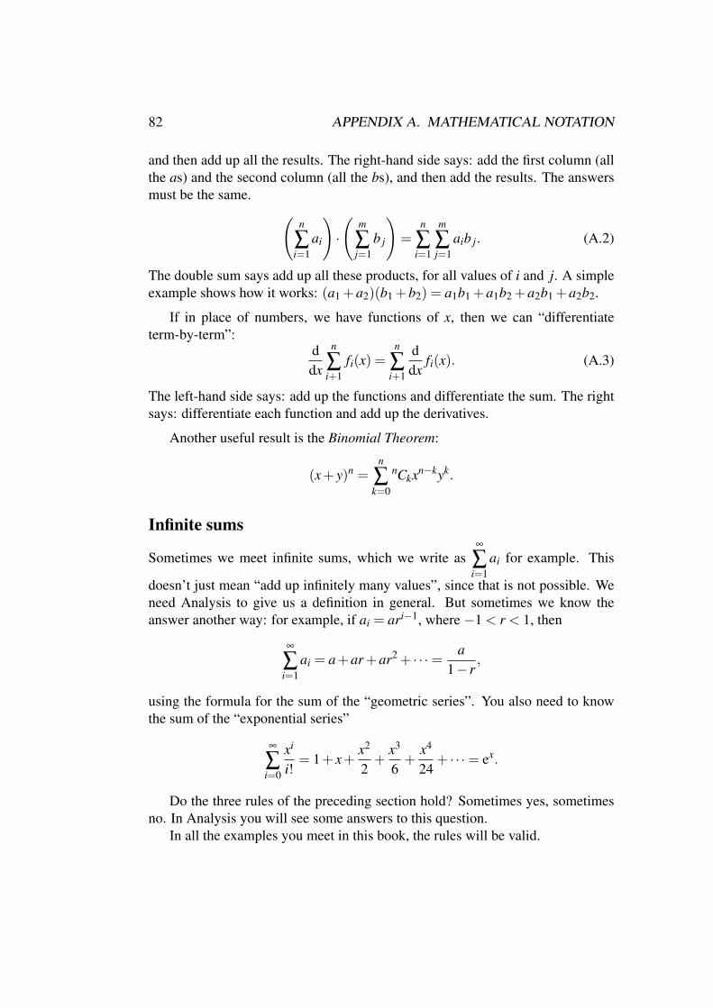
82 APPENDIX A. MATHEMATICAL NOTATION
and then add up all the results. The right-hand side says: add the first column (allthe as) and the second column (all the bs), and then add the results. The answersmust be the same. (
n
∑i=1
ai
)·
(m
∑j=1
b j
)=
n
∑i=1
m
∑j=1
aib j. (A.2)
The double sum says add up all these products, for all values of i and j. A simpleexample shows how it works: (a1 +a2)(b1 +b2) = a1b1 +a1b2 +a2b1 +a2b2.
If in place of numbers, we have functions of x, then we can “differentiateterm-by-term”:
ddx
n
∑i+1
fi(x) =n
∑i+1
ddx
fi(x). (A.3)
The left-hand side says: add up the functions and differentiate the sum. The rightsays: differentiate each function and add up the derivatives.
Another useful result is the Binomial Theorem:
(x+ y)n =n
∑k=0
nCkxn−kyk.
Infinite sums
Sometimes we meet infinite sums, which we write as∞
∑i=1
ai for example. This
doesn’t just mean “add up infinitely many values”, since that is not possible. Weneed Analysis to give us a definition in general. But sometimes we know theanswer another way: for example, if ai = ari−1, where −1 < r < 1, then
∞
∑i=1
ai = a+ar +ar2 + · · ·= a1− r
,
using the formula for the sum of the “geometric series”. You also need to knowthe sum of the “exponential series”
∞
∑i=0
xi
i!= 1+ x+
x2
2+
x3
6+
x4
24+ · · ·= ex.
Do the three rules of the preceding section hold? Sometimes yes, sometimesno. In Analysis you will see some answers to this question.
In all the examples you meet in this book, the rules will be valid.
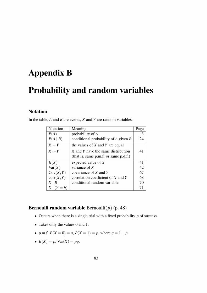
Appendix B
Probability and random variables
NotationIn the table, A and B are events, X and Y are random variables.
Notation Meaning PageP(A) probability of A 3P(A | B) conditional probability of A given B 24X = Y the values of X and Y are equalX ∼ Y X and Y have the same distribution 41
(that is, same p.m.f. or same p.d.f.)E(X) expected value of X 41Var(X) variance of X 42Cov(X ,Y ) covariance of X and Y 67corr(X ,Y ) correlation coefficient of X and Y 68X | B conditional random variable 70X | (Y = b) 71
Bernoulli random variable Bernoulli(p) (p. 48)
• Occurs when there is a single trial with a fixed probability p of success.
• Takes only the values 0 and 1.
• p.m.f. P(X = 0) = q, P(X = 1) = p, where q = 1− p.
• E(X) = p, Var(X) = pq.
83
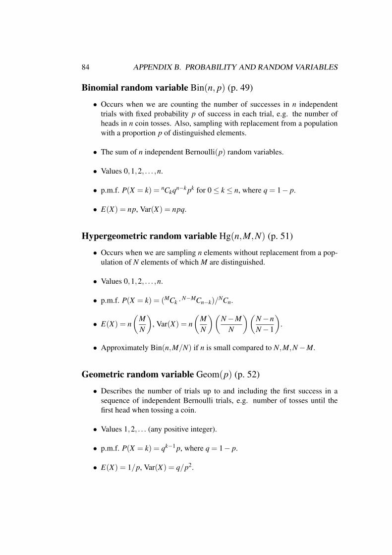
84 APPENDIX B. PROBABILITY AND RANDOM VARIABLES
Binomial random variable Bin(n, p) (p. 49)
• Occurs when we are counting the number of successes in n independenttrials with fixed probability p of success in each trial, e.g. the number ofheads in n coin tosses. Also, sampling with replacement from a populationwith a proportion p of distinguished elements.
• The sum of n independent Bernoulli(p) random variables.
• Values 0,1,2, . . . ,n.
• p.m.f. P(X = k) = nCkqn−k pk for 0 ≤ k ≤ n, where q = 1− p.
• E(X) = np, Var(X) = npq.
Hypergeometric random variable Hg(n,M,N) (p. 51)
• Occurs when we are sampling n elements without replacement from a pop-ulation of N elements of which M are distinguished.
• Values 0,1,2, . . . ,n.
• p.m.f. P(X = k) = (MCk ·N−MCn−k)/NCn.
• E(X) = n(
MN
), Var(X) = n
(MN
)(N−M
N
)(N−nN−1
).
• Approximately Bin(n,M/N) if n is small compared to N,M,N−M.
Geometric random variable Geom(p) (p. 52)
• Describes the number of trials up to and including the first success in asequence of independent Bernoulli trials, e.g. number of tosses until thefirst head when tossing a coin.
• Values 1,2, . . . (any positive integer).
• p.m.f. P(X = k) = qk−1 p, where q = 1− p.
• E(X) = 1/p, Var(X) = q/p2.
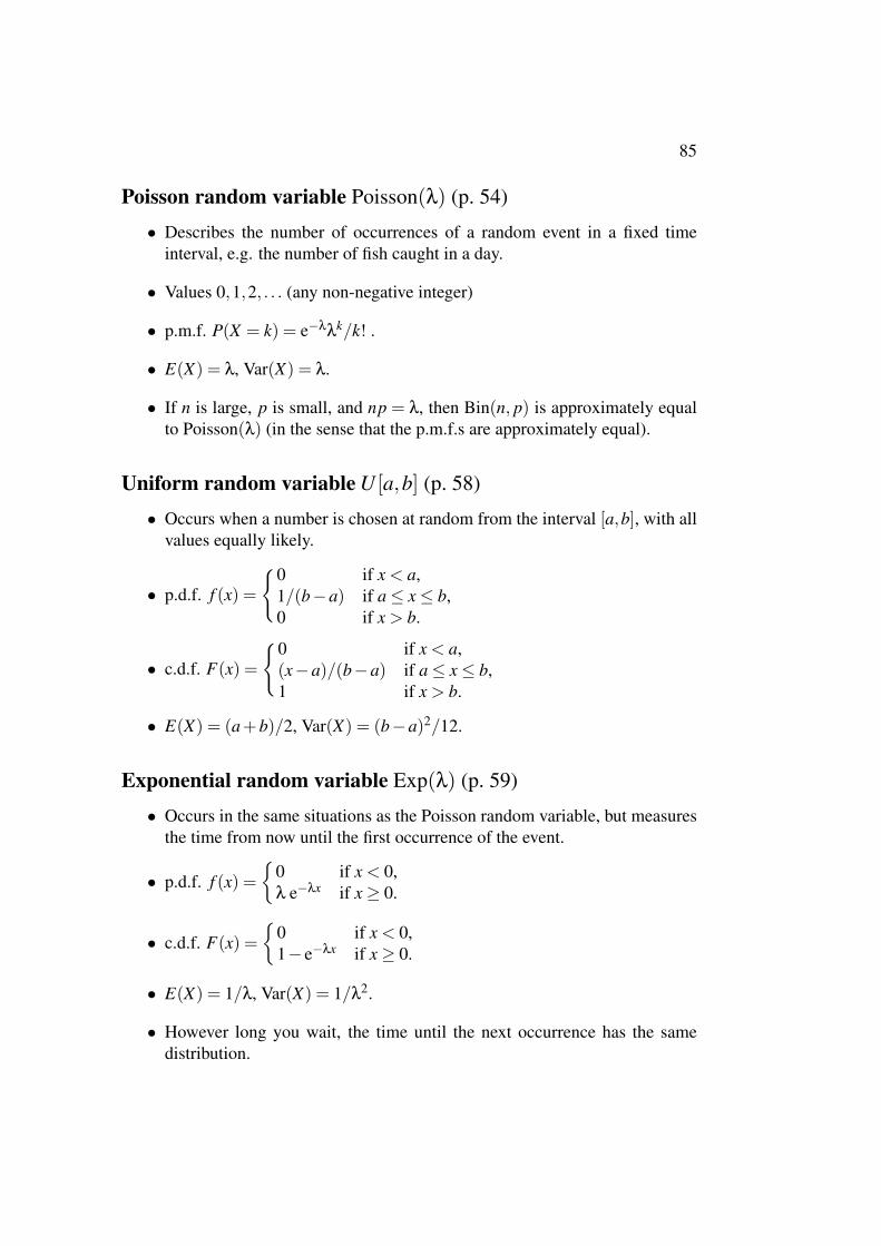
85
Poisson random variable Poisson(λ) (p. 54)
• Describes the number of occurrences of a random event in a fixed timeinterval, e.g. the number of fish caught in a day.
• Values 0,1,2, . . . (any non-negative integer)
• p.m.f. P(X = k) = e−λλk/k! .
• E(X) = λ, Var(X) = λ.
• If n is large, p is small, and np = λ, then Bin(n, p) is approximately equalto Poisson(λ) (in the sense that the p.m.f.s are approximately equal).
Uniform random variable U [a,b] (p. 58)
• Occurs when a number is chosen at random from the interval [a,b], with allvalues equally likely.
• p.d.f. f (x) =
0 if x < a,1/(b−a) if a ≤ x ≤ b,0 if x > b.
• c.d.f. F(x) =
0 if x < a,(x−a)/(b−a) if a ≤ x ≤ b,1 if x > b.
• E(X) = (a+b)/2, Var(X) = (b−a)2/12.
Exponential random variable Exp(λ) (p. 59)
• Occurs in the same situations as the Poisson random variable, but measuresthe time from now until the first occurrence of the event.
• p.d.f. f (x) =
0 if x < 0,λ e−λx if x ≥ 0.
• c.d.f. F(x) =
0 if x < 0,1− e−λx if x ≥ 0.
• E(X) = 1/λ, Var(X) = 1/λ2.
• However long you wait, the time until the next occurrence has the samedistribution.
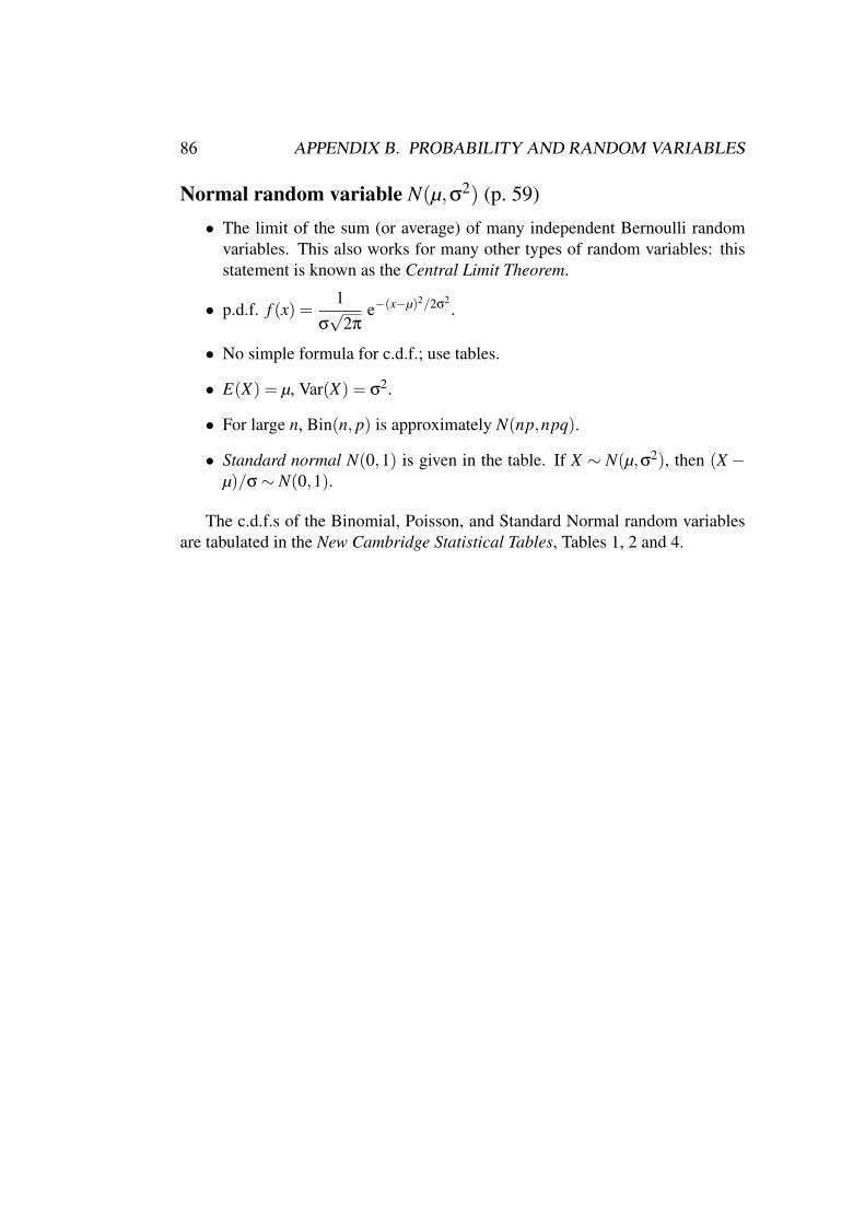
86 APPENDIX B. PROBABILITY AND RANDOM VARIABLES
Normal random variable N(µ,σ2) (p. 59)
• The limit of the sum (or average) of many independent Bernoulli randomvariables. This also works for many other types of random variables: thisstatement is known as the Central Limit Theorem.
• p.d.f. f (x) =1
σ√
2πe−(x−µ)2/2σ2
.
• No simple formula for c.d.f.; use tables.
• E(X) = µ, Var(X) = σ2.
• For large n, Bin(n, p) is approximately N(np,npq).
• Standard normal N(0,1) is given in the table. If X ∼ N(µ,σ2), then (X −µ)/σ ∼ N(0,1).
The c.d.f.s of the Binomial, Poisson, and Standard Normal random variablesare tabulated in the New Cambridge Statistical Tables, Tables 1, 2 and 4.