storm water runoff detention basin designco2.coe.utah.edu/cveen4410b/pdf/samplereport1.pdfstorm...

Storm Water Runoff

Detention Basin Design Medrum Building, University of Utah

CVEEN 4410 Engineering Hydrology, Spring 2012

Submitted by

Executive Summary

Urbanization has a significant impact on the hydrologic cycle. The removal of natural vegetation

and construction of large sections of impervious areas decrease infiltration and increase the total

volume of storm water runoff. In addition the peak runoff discharge rate increases in intensity

and timing. If these effects are not addressed, flooding of urban areas will occur which can be

costly and dangerous for area residents. Also increased intensity of peak discharge negatively

affects natural waterways, decreasing water quality in the process. Water quality is also

degraded due to the storm water gathering pollutants off the urban impervious surfaces and then

transporting it to water bodies were the storm water enters untreated.

In an attempt to mitigate the negative effects of urbanization on the hydrology of a watershed

storm water control methods are used. This report provides the analysis of the watershed which

has its outlet 100 feet downstream of the MCE Building on the University of Utah Campus. By

determining the pre-development hydrologic conditions a design can be provided that will

account for the effects of urbanization. For this project a detention basin is proposed. The basin

will detain the storm water runoff and then release it at rates that will be equal to or less than the

pre-development peak discharge rates.

This report consists of 4 sections: the pre-development watershed analysis, an in-depth analysis

of an impervious urban structure within the watershed, the post-development watershed analysis,

and the detention basin design. Also included are Appendices which provided detailed

information on the analysis methods used. The final product is a design which accomplishes the

stated goal of mimicking the pre-development hydrology within the urban environment.

3 | P a g e

Table of Contents

Executive Summary ....................................................................................................................... 2

1. Introduction ........................................................................................................................ 7

1.2 Problem Description .......................................................................................................... 7

1.3 Goals & Objectives ............................................................................................................ 7

2. Pre-Development Watershed Analysis ............................................................................. 7

2.1 Purpose of Analysis ............................................................................................................ 8

2.2 Pre-development Watershed Properties .......................................................................... 9

2.3 Time of Concentration ..................................................................................................... 15

2.4 Peak Discharge via the Rational Method ....................................................................... 15

2.5 Predicted Hydrographs via HEC-HMS ......................................................................... 15

3. Building Drainage Parameters, MCE Case Study ........................................................ 16

3.1 Purpose of Analysis .......................................................................................................... 17

3.2 Roof Properties ................................................................................................................. 17




3.6 Summary of Roof Hydrologic Parameters ................................................................... 21

4. Post-Development Watershed Analysis ........................................................................ 22

4.1 Purpose of Analysis .......................................................................................................... 22

4.2 Post-development Watershed Properties ....................................................................... 22




5. Detention Basin Design .................................................................................................... 29

5.1 Required Detention Basin Size........................................................................................ 29

5.2 Detention Basin Design .................................................................................................... 29

5.3 Outlet Structure Design ................................................................................................... 31

5.4 Pipe Requirements for Detention Basin Inflow/Outflow .............................................. 32

6. Summary and Conclusions .............................................................................................. 32

References ..................................................................................................................................... 33

4 | P a g e

Appendices ................................................................................................................................... 34

A. SCS Curve Number Method .......................................................................................... 34

B. Salt Lake City Precipitation Data .................................................................................. 35

C. Time of Concentration Method ...................................................................................... 36

D. Time of Concentration Calculation – Pre-Development Watershed ........................... 39

E. Rational Method ................................................................................................................ 41

F. HEC-HMS Method ........................................................................................................... 42

G. HEC-HMS Analysis – Pre-Development Watershed ..................................................... 44

H. HEC-HMS Analysis – MCE Building Case Study ........................................................ 46

I. HEC-HMS Analysis – Post-Development Watershed ..................................................... 48

J. HEC-HMS Analysis – Detention Basin ................................................................................ 50

5 | P a g e

List of Figures and Tables

Figure 1: Developed versus Natural Hydrograph .................................................................................... 8

Figure 2: Watershed Map with Sub-Areas ............................................................................................... 9

Figure 3: Watershed Total Area Calculation ......................................................................................... 10

Figure 4: Sub-Watershed Area Calculations .......................................................................................... 10

Table 1: Table 2-2d from USDA TR55 guide ......................................................................................... 11

Figure 5: Historical Photo of the Area .................................................................................................... 11

Figure 6: USDA Soil Survey ..................................................................................................................... 12

Table 2: Curve Number Detail Summary ............................................................................................... 12

Table 3: Table 3-1 from USDA TR55 guide (USDA, 1986) ................................................................... 13

Table 4: SCS Method Detail Summary ................................................................................................... 14

Table 5: Runoff Coefficients .................................................................................................................... 14

Table 6: Rational Method Peak Discharge Rates................................................................................... 15

Table 7: Comparison of Peak Discharge Rates from the Rational Method and HEC-HMS ............. 16

Figure 7: MCE Roof Architectural Plan ................................................................................................. 16

Table 8: MCE Roof, Area Summary ....................................................................................................... 17

Table 9: Table 2-2a from USDA TR55 guide ......................................................................................... 18

Table 10: Runoff Coefficient Detail Summary ...................................................................................... 19

Table 11: Time of Concentration Worksheet ......................................................................................... 19

Table 12: Peak Discharge for Each Sub-Watershed .............................................................................. 20

Table13: Peak Discharge Entire Roof Section ....................................................................................... 20

Table 14: Roof Hydrologic Parameters .................................................................................................. 21

Figure 8: Post-development sub-watersheds .......................................................................................... 23

Figure 9: Post-Development Watershed Area Calculations .................................................................. 23

Table 15: Post-Development Watershed Curve Number Detailed Summary ..................................... 24

Table 16: Post-Development Watershed Manning’s Roughness Coefficients ..................................... 25

Table 17: SCS Method Detailed Summary ............................................................................................. 25

Table 18: Time of Concentration Worksheet ......................................................................................... 26

Table 19: Peak Discharge for Each Sub-Watershed .............................................................................. 27

Table 20: Peak Discharge for Entire Post-Development Watershed ................................................... 28

Table 21: Comparison of Peak Discharge Rates from the Rational Method and HEC-HMS ........... 28

Figure 10: Detention Basin Location ....................................................................................................... 30

6 | P a g e

Figure 11: Conceptual Drawing of Detention Basin Design (NOTE: drawing not to scale) .............. 30

Figure 12: Example of an Outlet Structure ............................................................................................ 31

Figure 13: Conceptual Drawing of Outlet Structure Design (NOTE: drawing not to scale) ............. 31

Table 22: Inflow and Outflow Pipe Diameter Requirements ................................................................ 32

Figure 14: Chart for Estimating Velocity from TR-55 (USDA, 1986) ................................................. 37

Figure 15: Time of Concentration Worksheet from TR55 Guide ........................................................ 38

Figure 16: Time of Concentration, Path Lengths for Area 2 and Area 3 ............................................ 40

Figure 17: Time of Concentration, Path Length for Area 1 ................................................................. 40

Table 23: Runoff Coefficients .................................................................................................................. 41

Figure 18: HEC-HMS Standard View Screen ........................................................................................ 43

Figure 19: HEC-HMS Watershed Model ............................................................................................... 44

Table 24: HEC-HMS Results, 5 year, 25 year, & 100 year storms ....................................................... 44

Figure 20: 5 year storm hydrograph ....................................................................................................... 45

Figure 21: 25 year storm hydrograph ..................................................................................................... 45

Figure 22: 100 year storm hydrograph ................................................................................................... 45

Figure 23: HEC-HMS Watershed Model for MCE Rooftop ................................................................ 46











Table 27: HEC-HMS Results, 100-year storm ....................................................................................... 50

Figure 32: Detention Basin Storage Table and Volume Graph Vs. Time ............................................ 51

Figure 33: Outlet Structure, Flow from 4 levels of Orifices .................................................................. 51

7 | P a g e

1. Introduction

Runoff is part of the hydrologic cycle, which also includes precipitation, infiltration, evaporation,

transpiration, and ground water flow. The control of runoff in developed areas must be

addressed so that damage from flooding does not occur. Engineers are tasked with developing

designs to control storm water runoff. The first step of this design is to perform hydrologic

analysis to determine the direct runoff, which is equal to the net precipitation over a watershed

area. The definition of a watershed is “a contiguous area that drains to an outlet, such that

precipitation that falls within the watershed runs off through that single outlet.” (Bedient, pg. 8).

Net precipitation is the difference between total rain volume and the discharge volume. The

difference in these values includes losses to interception, depression storage, infiltration,

evaporation, and transpiration. It is the discharge volume, or direct runoff, which must be

managed with effective drainage design measures.

1.2 Problem Description

The Meldrum Civil Engineering (MCE) Building is located on the University of Utah Campus in

Salt Lake City, Utah. The watershed that contributes runoff to the MCE Building must be

analyzed, so a point 100 feet downstream, or west, of the MCE Building will be the point of

analysis for this design. State-of-the-art hydrologic analysis methods are utilized to design

containment and processing of storm water runoff that results from the contributing watershed at

this point of analysis.

1.3 Goals & Objectives

The goal of this design is to provide the necessary parameters for construction of a detention

basin that will control storm water runoff at the point of analysis. A detention basin is a storm

water management tool used to capture and temporarily detain storm water to prevent excessive

discharge or flooding. In order to develop the detention basin design several steps will be taken

including a pre-development watershed analysis, the analysis of drainage parameters for

buildings within the watershed, and a post-development analysis. The results of these steps will

provide the data necessary to design the detention basin for this system.

2. Pre-Development Watershed Analysis

The first step in designing a detention basin to control runoff from the watershed area with an

outlet at the MCE building was to determine the boundaries of this watershed and the pre-

development conditions. The boundaries of the watershed are decided by determining the area

8 | P a g e

that drains to the point of analysis, which it the point 100 feet downstream of the MCE building.

Pre-development conditions describe the area prior to any development of the land for human

use. This is also referred to as the natural condition of the area.

2.1 Purpose of Analysis

The urbanization of areas leads to decreased infiltration of precipitation due to the replacement

of natural vegetation with impervious surfaces such as rooftops, parking lots, and roadways.

Runoff travel times decrease as the natural vegetation is replaced by impervious surfaces and

interception due to vegetation and natural depression storage is removed. These modifications of

the natural landscape cause increased peak discharge rates and a larger overall volume of runoff.

A hydrograph is a graph which plots runoff discharge over time. The effect of urbanization is a

post-development direct runoff (DRO) hydrograph that peaks higher and more quickly than the

pre-development DRO hydrograph (see Figure 1). The purpose of pre-development watershed

analysis is so that in the final design drainage systems can be created that match peak discharge

flows from the developed area to what they were prior to development. In other words, to create

a drainage management system in the form of a detention basin that forces the post-development

hydrograph peak to be less than or equal to the pre-development hydrograph peak, per local

ordinances. Because the goal of the design is to mimic hydrological pre-development

conditions, it is necessary to determine what those pre-development conditions were.

Figure 1: Developed versus Natural Hydrograph

9 | P a g e

2.2 Pre-development Watershed Properties

The watershed area, with the point of discharge 100 feet west of the MCE building, was

delineated using a combination of a raised-relief map and Google © earth maps. This watershed

was divided into 3 sub-watersheds because of differences in geographical conditions of the area

resulting in variations in types of vegetation. The division into sub-watersheds results in a more

accurate analysis due to the fact that different surface conditions lead to different runoff amounts

and runoff travel times, which will be seen in following calculations. The most important factor

in determining volume of runoff is the surface area over which precipitation collects. The area

of this watershed and sub-watersheds were calculated to be 311 acres overall; 162 acres for area

1, 64 acres for area 2, and 85 acres for area 3. See figures 2 through 4 for detail.

Figure 2: Watershed Map with Sub-Areas

10 | P a g e

Figure 3: Watershed Total Area Calculation

Figure 4: Sub-Watershed Area Calculations

Pre-development characteristics of this area, a critical aspect of the analysis, were determined.

These characteristics include assigned values for curve number, roughness coefficients, and

runoff coefficients, which are necessary to estimate peak discharge, DRO hydrographs, and total

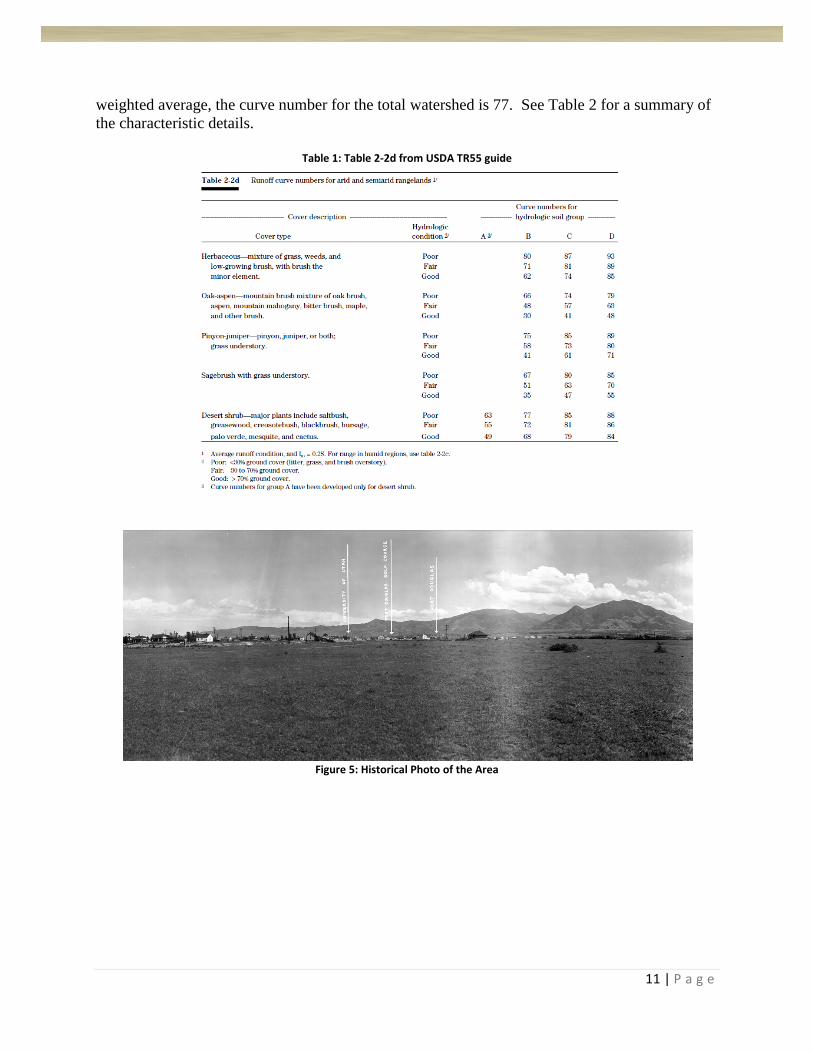
volume of runoff. According to the USDA guide TR-55 (USDA,1986), the runoff curve number

(CN) is based on soil types, plant cover, amount of impervious areas, interception, and surface

storage. Table 2-2d (USDA,1986) in this guide was used to determine the curve number for the

watershed (see Table 1). The pre-development cover type was determined from historical photos

(Figure 5) and current satellite imagery of non-developed sections found using Google Earth.

Using a soil classification of C (from USDA soil surveys, see Figure 6), a cover type of oak

aspen, and hydrologic condition of poor, the curve number was found to be 74 for sub-

watersheds 2 and 3. For sub-watershed 1, soil C, a cover type of sagebrush with grass, and

hydrologic condition of poor, suggests the curve number to be approximately 80. Using a

11 | P a g e

weighted average, the curve number for the total watershed is 77. See Table 2 for a summary of

the characteristic details.

Table 1: Table 2-2d from USDA TR55 guide

Figure 5: Historical Photo of the Area

12 | P a g e

Figure 6: USDA Soil Survey

Table 2: Curve Number Detail Summary

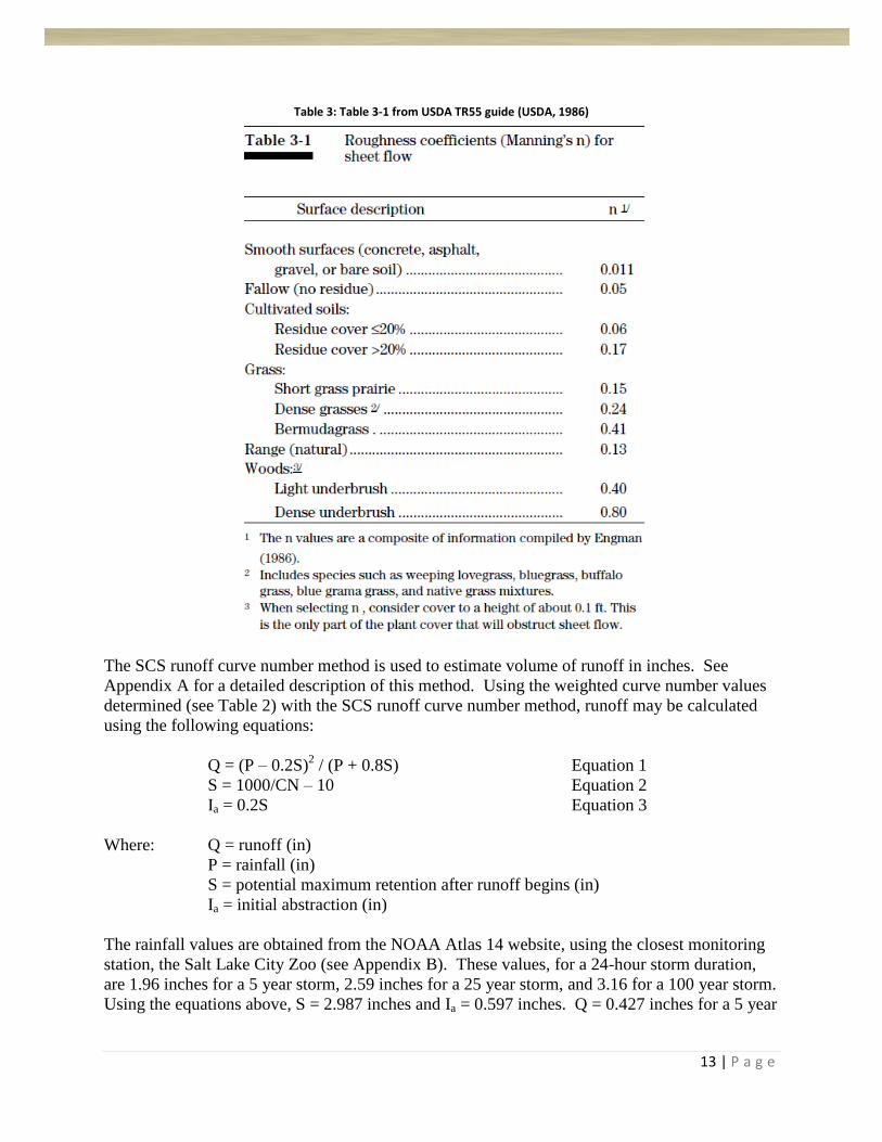
Manning’s roughness coefficients (n) are used in calculating the time it takes for water to flow

through the watershed, which is referred to as time of concentration. They are related to the

vegetation of the surface area up to 0.1 foot off the ground. These values are listed in table 3-1

in the TR-55 guide (see Table 3). For area 1 the coefficient is 0.15 (short grass) and for areas 2

and 3 the coefficient is 0.40 (light underbrush).

Sub-Watersheds Cover Type Hydrologic Condition Soil Group Curve Number Area (acres)

Area 1 Sagebrush/Grass Poor C 80 162

Area 2 Oak Aspen Poor C 74 64

Area 3 Oak Aspen Poor C 74 85

Total Watershed Area = 311

Weighted Average = [(162 * 80) + (64 * 74) + (85 * 74)] / 311

Curve Number for Watershed = 77

13 | P a g e

Table 3: Table 3-1 from USDA TR55 guide (USDA, 1986)

The SCS runoff curve number method is used to estimate volume of runoff in inches. See

Appendix A for a detailed description of this method. Using the weighted curve number values

determined (see Table 2) with the SCS runoff curve number method, runoff may be calculated

using the following equations:

Q = (P – 0.2S)2 / (P + 0.8S) Equation 1

S = 1000/CN – 10 Equation 2

Ia = 0.2S Equation 3

Where: Q = runoff (in)

P = rainfall (in)

S = potential maximum retention after runoff begins (in)

Ia = initial abstraction (in)

The rainfall values are obtained from the NOAA Atlas 14 website, using the closest monitoring

station, the Salt Lake City Zoo (see Appendix B). These values, for a 24-hour storm duration,

are 1.96 inches for a 5 year storm, 2.59 inches for a 25 year storm, and 3.16 for a 100 year storm.

Using the equations above, S = 2.987 inches and Ia = 0.597 inches. Q = 0.427 inches for a 5 year

14 | P a g e

storm, 0.797 inches for a 25 year storm, and 1.183 inches for a 100 year storm. See Table 4 for a

detailed summary of results.

Table 4: SCS Method Detail Summary

The runoff coefficient (C) is defined as the ratio of runoff to precipitation. Estimated values of C

are used with the Rational Method to estimate peak discharge. The runoff volumes (Q) and the

precipitation values (Ia) from Table 4 were used to calculated the C values. The average runoff

coefficient for this area is the ratio of the average of the calculated Q values to the average of the

Ia values, which equals 0.30. Detailed results are included in Table 4. The calculated C values

were compared with values that have been empirically derived. Table 5 provides these values.

This comparison provides concurrence that the runoff coefficients calculated in Table 4 are

within the average range.

Table 5: Runoff Coefficients

CN P (in) S (in) Ia (in) Q (in) C

24 hour, 5 year storm 77 1.96 2.987 0.597 0.427 0.218

24 hour, 25 year storm 77 2.59 2.987 0.597 0.797 0.308

24 hour, 100 year storm 77 3.16 2.987 0.597 1.183 0.374

15 | P a g e

2.3 Time of Concentration

Time of concentration (tc) is the time required for water to flow from the most hydraulically

distant point in a watershed to the watershed outlet, which in this analysis is the MCE building.

Time of concentration is necessary information for calculating the peak discharge using the

rational method, and is also necessary for specifying lag-time data associated with SCS methods

utilized by the HEC-HMS program; results of both methods are discussed in more detail in

subsequent sections of this report. The roughness coefficients determined earlier (Table 3) as

well as the slope of the watershed for the anticipated flow path, which was determined using

Google Maps ©, are used for these calculations. The TR-55 guide (USDA, 1986) provides a

worksheet to calculate time of concentration which includes a summation of travel time values

corresponding to sheet flow, shallow concentrated flow, and channel flow. For this watershed

the time of concentration for the entire watershed was determined to be 0.97 hours. See

Appendix C for a complete description of the method used to estimate times of concentration and

Appendix D for details of calculations for the pre-development watershed.

2.4 Peak Discharge via the Rational Method

The rational method is used to determine peak discharge rates (Qp) by relating rainfall to runoff.

The formula for this method is Qp = CiA, where C = runoff coefficient, i = intensity of rainfall of

chosen frequency for a duration equal to the time of concentration (in/hr), and A = area of the

watershed (acres). See Appendix E for a complete explanation of this method. Because the time

of concentration for this watershed is just under one hour (0.97 hours), the NOAA Atlas 14 (see

Appendix B) 1 hour storm data was used in this calculation. These values are .714 inches for the

5 year storm, 1.18 for the 24 year storm, and 1.77 for the 100 year storm. The peak discharge

rates for this watershed were determined to be 48 cfs for the 5-year storm, 113 cfs for the 25-year

storm, and 206 for the 100-year storm. See table 6 for detail of calculations.

Table 6: Rational Method Peak Discharge Rates

2.5 Predicted Hydrographs via HEC-HMS

HEC-HMS was used to model three storms; 5-year, 25-year, and 100-year. See Appendix F for

a complete discussion of HEC-HMS methods. Complete results of these analyses are listed in

appendix G. The peak discharge rates for the watershed, which is listed as the discharge for the

MCE Building, are as follows: 5 year storm equals 65 cfs, 25 year storm equals 138.6 cfs, 100

year storm equals 215.4 cfs. See Table 7 for these results in comparison to results obtained with

the Rational Method.

A (acres) i (in/hr) C Qp (cfs)

5 year Storm 311 0.714 0.218 48

25 year Storm 311 1.18 0.308 113

100 year Storm 311 1.77 0.374 206

16 | P a g e

While the Rational Method and HEC-HMS are both widely used and well accepted methods for

use in watershed analysis and the design of storm water systems, each has its limitations. The

rational method is more accurate when used for smaller, semi-urbanized areas. Because of the

degree of detail and ability to adjust over time, HEC-HMS provides more accurate results for

larger watersheds. Because of this the results from HEC-HMS are assumed to more accurate for

this case and will be used in further calculations for this project.

Table 7: Comparison of Peak Discharge Rates from the Rational Method and HEC-HMS

3. Building Drainage Parameters, MCE Case Study

The next step, after the analysis of the pre-development watershed, is to perform an analysis of

the drainage parameters for the buildings within the watershed. Although the most accurate

method would be to perform this analysis on every building that falls within the drainage area, a

less time intensive and still appropriately accurate technique is to perform a case study of one

building. For this design that building will be the MCE building, specifically, the recent addition

to the northwest corner for which plans are readily available (see Figure 7).

Figure 7: MCE Roof Architectural Plan

Rational Method HEC-HMS

5 year Storm 48 65

25 year Storm 113 138.6

100 year Storm 206 215.4

Qp (cfs)

17 | P a g e


As with the analysis of the pre-development watershed, time of concentration, peak discharge,

total volume of runoff, and the runoff hydrograph for the building rooftop area must be

determined. Once these values are established then assumptions can be made for other surfaces

within the post-development watershed. As stated, the post-development watershed could be

broken into hundreds of sub-watersheds and analysis could be performed on each. However in

addition to the impractical time requirements, this would not necessarily provide any more

accurate results. By providing an in depth analysis of one rooftop, necessary parameters can be

established for use in similar impervious areas within the developed watershed. With this

information educated assumptions can be made that result in accurate estimates of post-

development peak discharge and DRO hyrdrographs.

.

3.2 Roof Properties

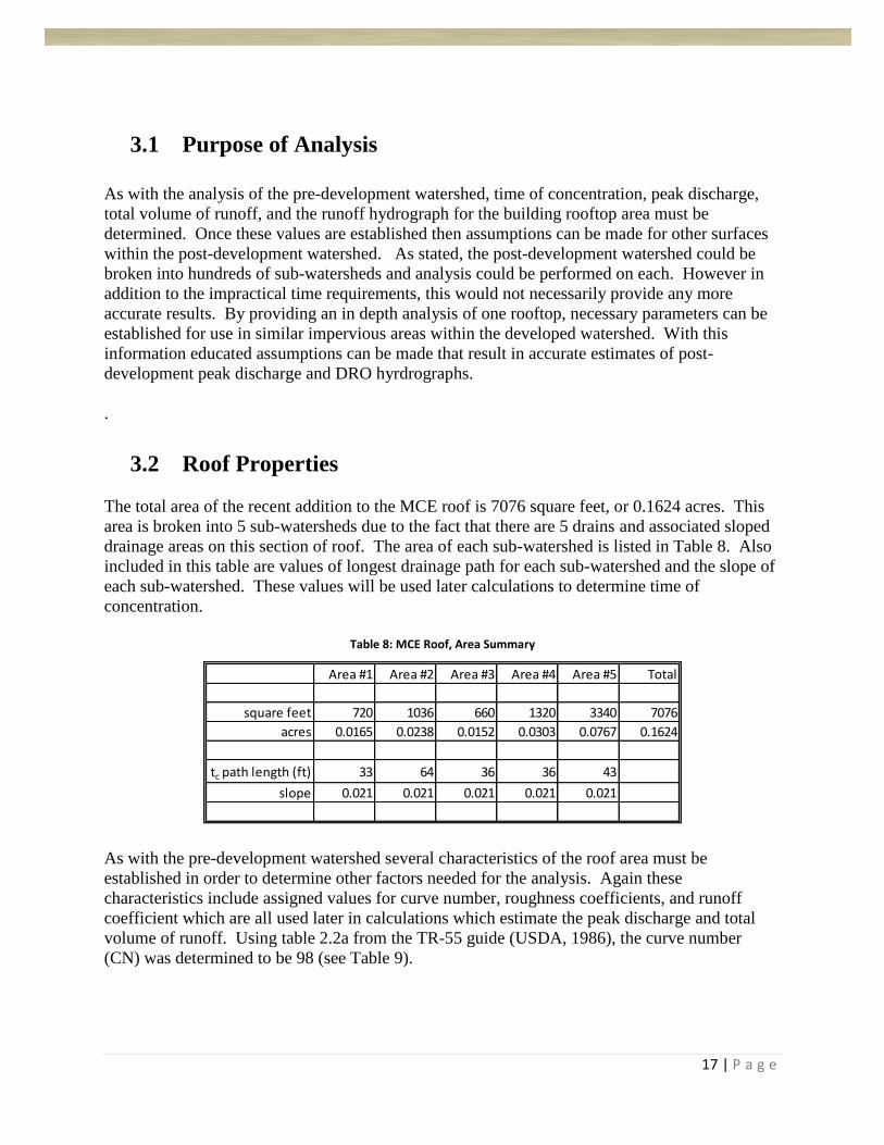
The total area of the recent addition to the MCE roof is 7076 square feet, or 0.1624 acres. This

area is broken into 5 sub-watersheds due to the fact that there are 5 drains and associated sloped

drainage areas on this section of roof. The area of each sub-watershed is listed in Table 8. Also

included in this table are values of longest drainage path for each sub-watershed and the slope of

each sub-watershed. These values will be used later calculations to determine time of

concentration.

Table 8: MCE Roof, Area Summary

As with the pre-development watershed several characteristics of the roof area must be

established in order to determine other factors needed for the analysis. Again these

characteristics include assigned values for curve number, roughness coefficients, and runoff

coefficient which are all used later in calculations which estimate the peak discharge and total

volume of runoff. Using table 2.2a from the TR-55 guide (USDA, 1986), the curve number

(CN) was determined to be 98 (see Table 9).

Area #1 Area #2 Area #3 Area #4 Area #5 Total

square feet 720 1036 660 1320 3340 7076

acres 0.0165 0.0238 0.0152 0.0303 0.0767 0.1624

tc path length (ft) 33 64 36 36 43

slope 0.021 0.021 0.021 0.021 0.021

18 | P a g e

Table 9: Table 2-2a from USDA TR55 guide

The Manning’s roughness coefficient (n), used to calculate time of concentration, was

determined from table 3-1 in the TR55 guide (see Table 3 in this report). For a smooth surface

such as a rooftop this value is 0.011.

As with the pre-development analysis, the SCS runoff curve number method was used (see

Appendix A for a detailed description of this method). These calculations were performed using

the curve number of 98, equations 1, 2, and 3, and the rainfall values in Appendix B for a 5 year,

25 year, and 100 year storm. See Table 10 for a detail summary of results.

The runoff coefficient (C), which is the ratio of runoff to precipitation, is used to calculate peak

discharge in the rational method. This value was calculated using the runoff and precipitation

values obtained with the SCS method. The average runoff coefficient value for the three storms

was 0.91. Again this value was compared to the tabulated values in Table 5 which validated the

results.

19 | P a g e

Table 10: Runoff Coefficient Detail Summary


Time of concentration (tc) was calculated for each sub-watershed and for the overall watershed

(see Appendix C for detailed description of method). Because of the relatively short distances

from the most hydraulically remote point to the drain outlet in each of the roof sub-watersheds,

all flow is considered sheet flow. A modified version of the worksheet provided in the TR55

guide was used. The total time of concentration was calculated to be 0.0693 hours, or 4.2

minutes. See Table 11 for detail of calculations.

Table 11: Time of Concentration Worksheet


The Rational Method was used to calculate peak discharge values for the sub-watersheds and

overall roof area. See appendix E for a complete explanation of this method. The inputs to this

method include the area calculations listed in Table 6, the rainfall values obtained from the

NOAA Atlas-14 website as specified by the time of concentration, and the runoff coefficients as

determined previously. The peak discharge rates for each of the sub-watersheds are tabulated in

Table 12. The peak discharge rates for the entire roof section are 0.4 cfs for the 5-year storm, 0.7

cfs for the 25-year storm, and 1.0 cfs for the 100-year storm. See Table 13 for detail of results.


24 hour, 5 year storm 98 1.96 0.204 0.041 1.735 0.885

24 hour, 25 year storm 98 2.59 0.204 0.041 2.360 0.911

24 hour, 100 year storm 98 3.16 0.204 0.041 2.928 0.926

Worksheet 3: Time of Concentration (Tc) or travel time (Tt)Project: MCE Rooftop

Location: University of Utah

Sheet Flow

Segment ID #1 #2 #3 #4 #5

1 Surface descriptions (table 3-1) Smooth Surface Smooth Surface Smooth Surface Smooth Surface Smooth Surface

2 Manning's roughness coefficient, n (table 3-1) 0.011 0.011 0.011 0.011 0.011

3 Flow length, L (total L † 300 ft) ft 33 64 36 36 43

4 Two-year 24-hour rainfall, P2 in 1.64 1.64 1.64 1.64 1.64

5 Land slope, s ft/ft 0.021 0.021 0.021 0.021 0.021

6 Tt = 0.007 (nL) 0.8 Compute Tt hr 0.0114 0.0194 0.0122 0.0122 0.0141 0.0693

P20.5s0.4

⁺ ⁺ ⁺ ⁺ ⁼

20 | P a g e

Table 12: Peak Discharge for Each Sub-Watershed

Table13: Peak Discharge Entire Roof Section


5 year Storm 0.0165 2.724 0.885 0.040

25 year Storm 0.0165 4.5 0.911 0.068

100 year Storm 0.0165 6.756 0.926 0.103


5 year Storm 0.0238 2.724 0.885 0.057

25 year Storm 0.0238 4.5 0.911 0.098

100 year Storm 0.0238 6.756 0.926 0.149


5 year Storm 0.0152 2.724 0.885 0.037

25 year Storm 0.0152 4.5 0.911 0.062

100 year Storm 0.0152 6.756 0.926 0.095


5 year Storm 0.0303 2.724 0.885 0.073

25 year Storm 0.0303 4.5 0.911 0.124

100 year Storm 0.0303 6.756 0.926 0.190


5 year Storm 0.0767 2.724 0.885 0.185

25 year Storm 0.0767 4.5 0.911 0.314

100 year Storm 0.0767 6.756 0.926 0.480

Sub-Watershed #1

Sub-Watershed #2

Sub-Watershed #3

Sub-Watershed #4

Sub-Watershed #5


5 year Storm 0.1624 2.724 0.885 0.392

25 year Storm 0.1624 4.5 0.911 0.666

100 year Storm 0.1624 6.756 0.926 1.016

21 | P a g e


HEC-HMS was used to model the system for the three SCS design storms of 5, 25, and 100

years. This was done in order obtain peak discharge rates and produce direct runoff

hydrographs. See Appendix F for a complete discussion of this program. Results of this analysis

and runoff hydrographs for each storm are included in appendix H. The peak discharge for the

sub-watershed and entire roof section were comparable, although higher than what was found

with the Rational Method. These values are as follows: 5 year storm equals 0.293 cfs, 25 year

storm equals 0.367 cfs, and 100 year storm equals 0.472 cfs. Because the Rational Method was

specifically designed for small, urban watershed those results determined in the previous section

are more accurate than the results obtained from HEC-HMS.

3.6 Summary of Roof Hydrologic Parameters

A final tabulation of all results of the MCE roof top analysis was compiled. These results will be

used in further analysis of the developed area. The accuracy of the information obtained is

critical to the success of the detention basin design. See Table 14 for a summary of these

parameters.

Table 14: Roof Hydrologic Parameters

Curve Number Roughness Coefficient Surface Area (ft2) Surface Slope Time of Concentration

Area #1 98 0.011 720 0.021 0.0114

Area #2 98 0.011 1036 0.021 0.0194

Area #3 98 0.011 660 0.021 0.0122

Area #4 98 0.011 1320 0.021 0.0122

Area #5 98 0.011 3340 0.021 0.0141

22 | P a g e

4. Post-Development Watershed Analysis

The post-development watershed consists of the previously established geographic area which

contributes runoff to the point of analysis, which is the point 100 feet downstream of the MCE

building. The difference in this analysis, versus the pre-development watershed analysis, is that

in the post-development watershed the human modified landscape is considered. The existing

urbanized area with all the buildings, parking lots, roads, and other built land features are taken

into account in the determination of estimated peak discharge and DRO hydrographs.


As stated in the previous section, time of concentration, peak discharge, total volume of runoff,

and the runoff hydrograph for the post-development watershed must be determined. This

information is needed in order to establish the necessary design parameters for the detention

basin that will adjust for the differences between the resultant pre and post urbanization

hydrographs. This analysis provides the information necessary to reach the ultimate goal of the

detention basin design, which is to reduce peak discharge of the post-development watershed to

equal or less than the rate of the pre-development watershed.

4.2 Post-development Watershed Properties

As with the pre-development watershed, the post-development watershed was divided into sub-

watersheds. The sub-watersheds were determined using google maps ©. The delineations were

made based on the groupings of relatively similar types of land cover. For example, areas with a

higher percentage of impervious surfaces were separated from areas with a lower percentage of

impervious surfaces. In order to not need to treat every rooftop, parking lot, sidewalk, etc. as an

individual watershed, groupings were made of similar surfaced areas so that weighted curve

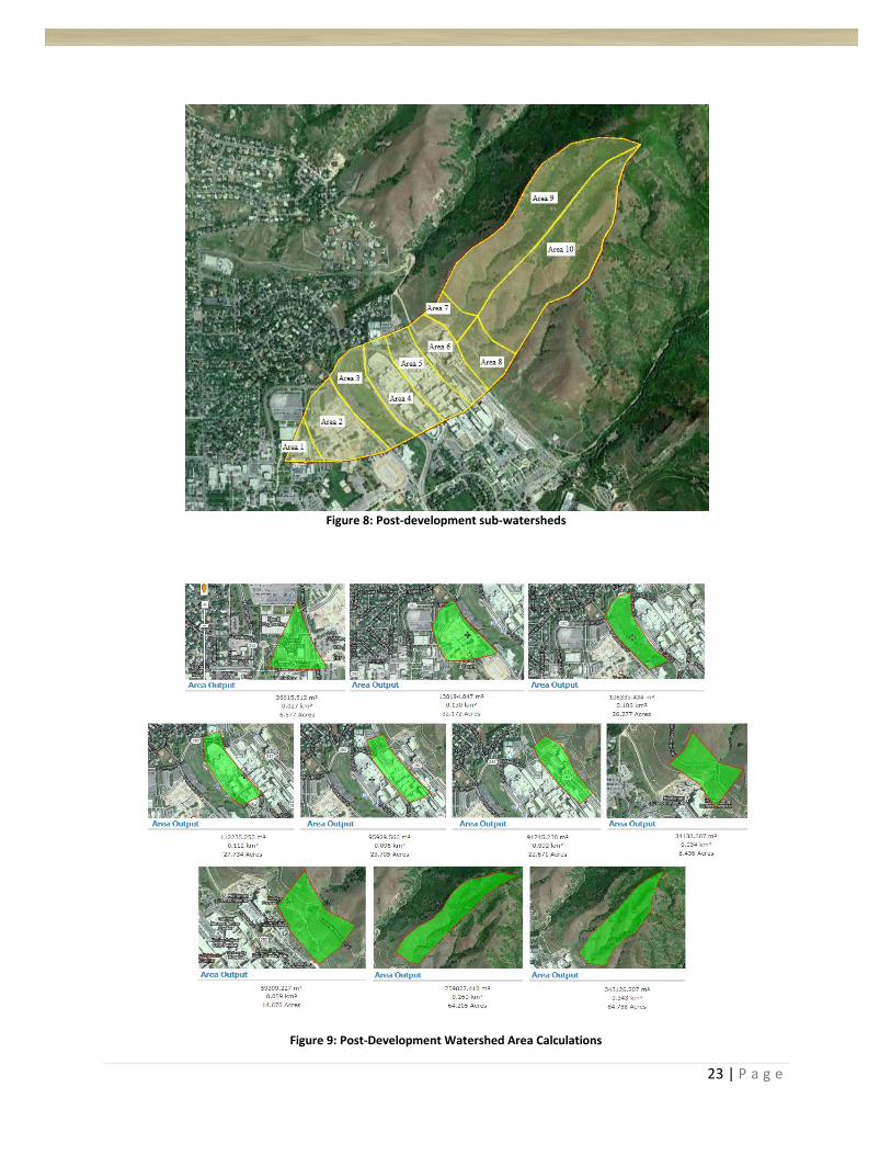
numbers could be assigned. Figure 8 shows the sub-watersheds, numbered 1 through 10. For

each of these sub-watersheds the area was calculated (see Figure 9). The area in acres for each

sub-watershed is listed in Table 15.

23 | P a g e

Figure 8: Post-development sub-watersheds

Figure 9: Post-Development Watershed Area Calculations

24 | P a g e

As with the pre-development watershed, certain characteristics of the areas were determined,

including curve number values, roughness coefficients, and runoff coefficients. The curve

numbers were determined using Table 2-2a from the TR-55 guide (USDA, 1983), which can be

found in Table 9 in this report. These values were weighted for each area in order to determine

an appropriate curve number for each sub-watershed. See Table 15 for details of this

determination and the resulting curve numbers for each area.

Table 15: Post-Development Watershed Curve Number Detailed Summary

The Manning’s roughness coefficients for each sub-watershed area were also determined. These

values are taken from TR-55 (USDA, 1983) (see Table 3) and will be used to calculate time of

concentration. These values were weighted as with the curve numbers. A tabulation of the

results is found in Table 16.

Sub-Watersheds Cover Type Percentage Hydrologic Condition Soil Group

Curve Number for

Cover/Condition

Weighted Curve

Number for Area Area (acres)

Lawns, Parks , etc. 50% Fair C 79

Paved, Roofs , Streets , etc. 50% N/A C 98











Area 7Sagebrush/Grass 100% Poor C 80

80 8.44

Area 8Sagebrush/Grass 100% Poor C 80

80 14.68

Area 9Oak Aspen 100% Poor C 74

74 64.21

Area 10Oak Aspen 100% Poor C 74

74 84.79

22.67

91

81

96

95

89

6.58

32.17

26.28

27.73

23.71

Curve Number for Watershed = 82

Total Watershed Area = 311

Weighted Average = [(6.58 * 89)+(32.17 * 91)+(26.28 * 81)+(27.73 * 96)+(23.71 * 95)+(22.67 * 89)+(8.44 * 80)+ (14.68 * 80)+(64.21 * 74)+ (84.79 * 74) ] / 311

Area 1

Area 2

Area 3

Area 4

Area 5

Area 6

89

25 | P a g e

Table 16: Post-Development Watershed Manning’s Roughness Coefficients

The SCS runoff curve number method was used to estimate volume of runoff in inches. See

Appendix A for a complete description of this method. The weighted curve number values from

Table 14 and precipitation values from NOAA Atlas 14, used in the pre-development SCS

method calculations, were used. The calculations produced the following results: S = 2.195

inches, Ia = 0.439 inches, and Q = 0.623 inches for a 5-year storm, 1.065 inches for a 25-year

storm, and 1.506 inches for a 100-year storm. See Table 17 for a detailed summary of results.

Table 17: SCS Method Detailed Summary

The runoff coefficient (C), which is used in the Rational Method to determine peak discharge,

was calculated using the results obtained from the SCS Method. The runoff coefficient is the

ratio of runoff to precipitation. The average runoff coefficient for the 5, 25, and 100-year storms

is 0.41. See Table 17 for detailed results. This value was compared to runoff coefficients that

have been empirically derived (see Table 5). This comparison provides concurrence that the

runoff coefficients calculated in Table 17 are within the average range.

Sub-Watersheds Surface Description Percentage

Coefficient for

Surface Type

Weighted

Coefficient for Area

Cultivated Soi ls 50% 0.17

Smooth Surface 50% 0.011











Area 7Short Grass 100% 0.15

0.15

Area 8Short Grass 100% 0.15

0.15

Area 9Light Underbrush 100% 0.4

0.40

Area 10Light Underbrush 100% 0.4

0.40

Area 5 0.03

Area 6 0.08

Area 3 0.15

Area 4 0.03

Area 1 0.09

Area 2 0.07


24 hour, 5 year storm 82 1.96 2.195 0.439 0.623 0.318

24 hour, 25 year storm 82 2.59 2.195 0.439 1.065 0.411

24 hour, 100 year storm 82 3.16 2.195 0.439 1.506 0.477

26 | P a g e


Time of concentration, the time required for water to flow from the most hydraulically distant

point in a watershed to the watershed outlet, was calculated for the post-development watershed.

See Appendix C for a complete description of this method. A modified version of the TR-55

(USDA, 1986) worksheet was used to calculate the travel time for each sub-watershed area and

the total time of concentration for the entire watershed. The time of concentration for the total

watershed was determined to be 0.90 hours or 54 minutes. See Table 18 for detail of

calculations. This decrease in time of concentration from the pre-development value is not

significant when considered for the entire watershed. However, when a comparison is made of

just the valley area, which is the developed portion of the watershed, the time of concentration

decreases by 28%, which is a drop from 13.6 minutes to 9.8 minutes.

Table 18: Time of Concentration Worksheet


The rational method, which is Qp = CiA, was used to determine the peak discharge rates (Qp) for

the developed watershed. See Appendix E for a description of the method. The runoff

coefficient values (C) from Table 17 were used with the area values (A) from Table 15. The

precipitation value (i) was obtained from the NOAA Atlas-14 table in Appendix B. Because the

time of concentration was 50 minutes the precipitation value was determined by interpolating.

The peak discharge rates for each of the sub-watersheds are tabulated in Table 19. The peak

discharge rates for the entire watershed are 79.3 cfs for the 5-year storm, 169.4 cfs for the 25-

year storm, and 294.9 cfs for the 100-year storm. See Table 20 for detail of results.

Worksheet 3: Time of Concentration (Tc) or travel time (Tt)Project: MCE Building

Location: University of Utah

Sheet Flow

Segment ID #1 #2 #3 #4 #5 #6 #7 / #8 #9 / #10

1 Surface descriptions (table 3-1) Light Underbrush

2 Manning's roughness coefficient, n (table 3-1) 0.40

3 Flow length, L (total L † 300 ft) ft 300

4 Two-year 24-hour rainfall, P2 in 1.64

5 Land slope, s ft/ft 0.12

6 Tt = 0.007 (nL) 0.8 Compute Tt hr ⁺ 0.5880 0.5880

P20.5s0.4

Shallow Concentrated Flow

Segment ID #1 #2 #3 #4 #5 #6 #7 / #8 #9 / #10

7 Surface description (paved or unpaved) Paved Paved Unpaved Paved Paved Paved Unpaved Unpaved

8 Flow length, L ft 638 921 494 604 552 603 698 4163

9 Watercourse slope, s ft/ft 0.08 0.08 0.12 0.12 0.12 0.18 0.2 0.3

10 Average velocity, V (figure 3-1) ft/s 6 6 5.5 7 7 8.5 7 9

11 Tt = L Compute Tt hr 0.0295 0.0426 0.0249 0.0240 0.0219 0.0197 0.0277 ⁺ 0.1285 0.3189

3600 V

Watershed Tc (Total of Tt from 6 and 11) 0.9069

⁼

⁼⁺ ⁺ ⁺ ⁺ ⁺ ⁺

⁺ ⁺ ⁺ ⁺ ⁺ ⁺

27 | P a g e

Table 19: Peak Discharge for Each Sub-Watershed


5 year Storm 6.58 0.802 0.318 1.67825 year Storm 6.58 1.325 0.411 3.583100 year Storm 6.58 1.988 0.477 6.240



















Sub-Watershed #7

Sub-Watershed #8

Sub-Watershed #9

Sub-Watershed #10

Sub-Watershed #1

Sub-Watershed #2

Sub-Watershed #3

Sub-Watershed #4

Sub-Watershed #5

Sub-Watershed #6

28 | P a g e

Table 20: Peak Discharge for Entire Post-Development Watershed


HEC-HMS was again used to model the system for the three SCS design storms of 5, 25, and

100 years. This was done to obtain peak discharge rate and direct runoff hydrographs. See

Appendix F for detailed information about HEC-HMS and Appendix I for results of this

analysis. The peak discharge rates for the watershed are as follows: 5 year storm equals 189 cfs,

25 year storm equals 278 cfs, 100 year storm equals 363 cfs. See Table 21 for these results in

comparison to results obtained with the Rational Method. The peak discharge rates obtained

using HEC-HMS are higher than those obtained with the Rational Method. As stated, the

Rational Method is more accurate when used for smaller, semi-urbanized areas. Because most of

this watershed is not yet developed, and because of the size, HEC-HMS is assumed to produce

more accurate results. In addition, designing for the HEC-HMS produced values is a more

conservative approach to take in sizing the detention basin.

Table 21: Comparison of Peak Discharge Rates from the Rational Method and HEC-HMS


5 year Storm 311.00 0.802 0.318 79.316

25 year Storm 311.00 1.325 0.411 169.363

100 year Storm 311.00 1.988 0.477 294.914

Rational Method HEC-HMS

5 year Storm 79 189

25 year Storm 169 278

100 year Storm 294 363

Qp (cfs)

29 | P a g e

5. Detention Basin Design

In order to adjust for the effects of urbanization on this watershed and account for the effects of

the built impervious surfaces on the natural hydrologic cycle, a detention basin is proposed. The

detention basin will temporarily detain storm water, and then release this storm water at a

determined rate in order to adjust for the quicker and more intense peak of the urbanized

hydrograph (see Figure 1). The detention basin will modify the outflow of storm water. The

peak discharge of the post-development watershed will be reduced to equal or less than the peak

discharge of the pre-development watershed.

5.1 Required Detention Basin Size

Using the following equation the approximate size of the detention basin was determined:

Vs = (Qpa - Qpb) * (tca) Equation 4

Where: Vs = Storage volume (ft3)

Qpa = Post-development peak discharge (cfs)

Qpb = Pre-development peak discharge (cfs)

tca = Post-development time of concentration (seconds)

The peak discharge rates used were values from HEC-HMS for the 100 year storm (see Tables 7

and 22). The result was a detention basin 480,911 ft3 or 11.04 acre-feet. A model was created in

HEC-HMS with a detention basin of 11.04 acre-feet. Through trial and error, and using the

detention basin and outlet structure as designed (see section 5.2 and 5.3), it was found that the

actual volume required was 9.27 acre-feet. At this volume the detention basin almost filled

during the 100-year storm event. Through the outlet structure the detained water was able to

drain at a maximum rate of 215 cfs. This peak discharge matches the peak discharge of the pre-

development watershed. See Appendix J for HEC-HMS inputs and results.

5.2 Detention Basin Design

For reasons of aesthetics the detention basin has been designed as an oval that will mimic the

shape of a natural water body. The basin will be 6 feet deep with a slope of 0.44 at the ends and

0.16 on the sides. At the necessary volume, the required surface area is 85,872 ft2. See Figure

10 for an image showing where the detention basin will be located. Figure 11 provides a

conceptual drawing of the detention basin with interior and exterior dimensions.

30 | P a g e

Figure 10: Detention Basin Location

Figure 11: Conceptual Drawing of Detention Basin Design (NOTE: drawing not to scale)

31 | P a g e

5.3 Outlet Structure Design

The outlet structure is designed to be constructed of concrete. It will be 6 feet tall and 5 foot by

5 foot wide. There will be 36 orifices total distributed equally on 3 sides. Each orifice will be

8.2 inches wide by 12” tall. The top of the structure will be open with a grate in case of storm

events greater than the 100-year storm. See Figure 12 for an example of a similar outlet

structure. See Figure 13 for a conceptual drawing of the structure for this project with

dimensions.

Figure 12: Example of an Outlet Structure

Figure 13: Conceptual Drawing of Outlet Structure Design (NOTE: drawing not to scale)

32 | P a g e

5.4 Pipe Requirements for Detention Basin Inflow/Outflow

Manning’s equation for pipe flow was used to calculate the required inflow and outflow pipe

diameters for the detention basin. The equation is:

d = [3.208 * n/Kn * Qp/(So1/2

)]3/8

Equation 5

Where: d = diameter (feet)

n = Manning’s roughness coefficient

Kn = constant, 1.49 for U.S. Customary Units

Qp = peak discharge (cfs)

So = slope

The recommended pipe is reinforced concrete pipe (RCP) which has a roughness coefficient of

0.015. The minimum recommended slope is 0.50. The peak discharge values used are for the

100-year storm. The results of these calculations show that a 7 foot diameter pipe is needed for

the inflow and a 6 foot diameter pipe is needed for the outflow. See detailed results in Table 22.

Table 22: Inflow and Outflow Pipe Diameter Requirements

6. Summary and Conclusions

The purpose of this design is to provide a measure in which the natural hydrology that existed in

the pre-developed watershed can be returned to the urbanized watershed. The method selected in

order to accomplish this goal is a detention basin. The information gathered provided data from

which the pre-development peak discharge rates for various storms could be determined. A

specific pervious area, the MCE rooftop, within the watershed was analyzed in detail. This

provided confirmation of assumptions, which were then used to make generalizations for the

post-development watershed so that peak discharge rates could be estimated. With this

information a detention basin and outlet structure have been designed which will temporarily

detain storm water runoff and allow it to drain at the pre-development peak rate. Through the

installation of this detention basin the goal to return the post-development watershed to pre-

development hydrological conditions will be achieved.

For Detention Basin Inflow For Detention Basin Outflow

Qp: 363 cfs Qp: 215 cfs

n: 0.015 n: 0.015

K: 1.49 K: 1.49

So: 0.50% So: 0.50%

d: 6.797283 feet d: 5.58515 feet

33 | P a g e

References

Huber, W.C., Bedient, P.B., Vieux, B.E., (2007), Hydrology and Floodplain Analysis, Place:

Publisher.

United States Department of Agriculture, Technical Release 55 (TR-55), Urban Hydrology for

Small Watersheds, June 1986

National Oceanic and Atmospheric Administration’s (NOAA) National Weather Service, Atlas

14 Point Precipitation Frequency Estimates, http://hdsc.nws.noaa.gov/hdsc/pfds/

34 | P a g e

Appendix A

SCS Curve Number Method

The SCS Curve Number Method was developed by the United State Department of Agriculture

(USDA) Natural Resources Conservation Service. The agency was formerly known as the Soil

Conservation Service or SCS. It is a method that is widely used for the predication of direct

runoff from storms. It is an empirical method developed by the USDA through the monitoring

and analysis of runoff from systems. It is a simple method to use and provides rough estimates

of the volume of runoff and infiltration.

The first step in this method is the identification of the appropriate curve number for the area to

be analyzed. The curve number is based on soil types, plant cover, amount of impervious areas,

interception, and surface storage. Curve numbers range from 30 to 98. Low numbers represent

lower runoff potential and more permeable surfaces while high numbers represent higher runoff

potential and more impervious surfaces. The TR55 guide published by the USDA includes a set

of four tables (Tables 2.2a through 2.2d) that are used to determine the curve number once the

other parameters have been determined.

The next step in this method is to determine the rainfall value. The selection of this value

depends on the duration and magnitude of design storm selected. Precipitation data is collected

by the National Oceanic and Atmospheric Administration (NOAA) and is available online at

http://dipper.nws.noaa.gov/hdsc/pfds/.

With values for the curve number and rainfall the calculations can be made. The equations are as

follows:

Q = (P – 0.2S)2 / (P + 0.8S) Equation 1

S = 1000/CN – 10 Equation 2

Ia = 0.2S Equation 3

Where: Q = runoff (in)

P = rainfall (in)

S = potential maximum retention after runoff begins (in)

Ia = initial abstraction (in)

The results from these equations are an estimated volume of runoff in inches (Q), an estimated

volume for initial abstractions in inches (Ia), and an estimated volume for potential maximum

retention in inches (S).

http://dipper.nws.noaa.gov/hdsc/pfds/

35 | P a g e

Appendix B

Salt Lake City Precipitation Data

36 | P a g e

Appendix C

Time of Concentration Method

Time of concentration (tc) is defined as the time required for water to flow from the most

hydraulically remote point in a watershed to the watershed outlet. It is an important parameter is

determining the response of a watershed to storm events. Time of concentration is dependent on

several factors including slope, distance, and surface conditions.

The method of segments is used to calculate time of concentration. This method consists of the

summation of three types of flow; sheet flow, shallow concentrated flow, and channel flow.

Sheet flow consists of the first 300 feet or less from the most remote point. The necessary

variables required to perform this calculation are the Manning’s roughness coefficient, which can

be found in Table 3-1 in the USDA TR-55 guide, the flow length, the two year, 24 hour rainfall

value for the area, and the land slope. With these values the following equation is used to

compute the time for this first section of flow.

T = (0.007 * (n * L)0.8

) / (P20.5

* s0.4

)

Where: T = time (hours)

n = Manning’s roughness coefficients

L = Flow length (ft)

P2 = Two-year 24-hour rainfall (in)

s = Land slope (ft/ft)

The next section of flow is shallow concentrated flow. The first step in this determining this

value is to determine the velocity of flow. This is done using the surface description of paved or

unpaved, the flow length, and the watercourse slope. From these variables the velocity can be

determined using figure 3-1 in the TR-55 guide (see Figure 14). Then the time is calculated

using the following equation:

T = L / (3600 * V)



V = Velocity (ft/s)

37 | P a g e

Figure 14: Chart for Estimating Velocity from TR-55 (USDA, 1986)

The next section is channel flow, which may or may not be relevant to every watershed. In the

situation that channel flow does occur the velocity must again be determined. In this case it is

determined by using the Manning’s equation for open channel flow. This equation is as follows:

V = (1.49 * r2/3

* s1/2

) / (n)

Where: V = Velocity (ft/s)

r = Hydraulic radius (ft)

s = Channel slope (ft/ft)

n = Manning’s roughness coefficient

38 | P a g e

Once the velocity is determined the time is calculated using the following equation:

T = L / (3600 * V)



V = Velocity (ft/s)

The total of the 3 calculated times are added together and this is the time of concentration for the

watershed. This method is detailed in the USDA TR55 guide. The guide also provides a

worksheet that can be used as a tool in organizing the calculations. See Figure 15 for a example

of the Time of Concentration Worksheet included in the TR55 guide.

Figure 15: Time of Concentration Worksheet from TR55 Guide

39 | P a g e

Appendix D

Time of Concentration Calculation – Pre-Development Watershed

40 | P a g e

Figure 16: Time of Concentration, Path Lengths for Area 2 and Area 3

Figure 17: Time of Concentration, Path Length for Area 1

41 | P a g e

Appendix E

Rational Method

The Rational Method is used to determine the peak discharge rate for a watershed. Peak

discharge is the highest rate of runoff resulting from a precipitation event. This value is

important to know for planning in order to avoid damage from flooding, to size storm water

management facilities, and to determine the effects of urbanization on the hydrology of a

watershed. The Rational Method provides a simple and quick method to calculate an

approximate peak discharge value. Following is the Rational Method equation:

Qp = CiA

where C = runoff coefficient

i = intensity of rainfall (in/hr)

A = area of the watershed (acres).

The runoff coefficient is the ratio of runoff to rainfall. There are charts available were these

coefficients can be obtained for various types of vegetation and cover (see Table 5 and Table 23

below). The coefficient can also be calculated if runoff and rainfall values are available. The

rainfall intensity needs to be selected for the storm duration that is the same time as the time of

concentration (see Appendix C for time of concentration method). The rainfall intensity can be

found at the NOAA Atlas-14 website. The area of the watershed needs to be in acres.

This method is very useful but does have some limitations. The method was developed for small

(100 acres or less) watersheds that are undergoing urbanization. Because of this the results are

not accurate when used for larger watersheds. The method assumes that rainfall intensity is

uniform over watershed and over duration of the storm event. It also assumes that runoff is

invariant with time, meaning that soil conditions do not change with time.

Table 23: Runoff Coefficients

42 | P a g e

Appendix F

HEC-HMS Method

HEC-HMS is a computer program designed for modeling hydrologic systems. It is a free

program that was developed by the United States Army Corps of Engineers (USACE).

According to the USACE web page “the primary goal of HEC is to support the nation in its

water resources management responsibilities by increasing the Corps technical capability in

hydrologic engineering and water resources planning and management. An additional goal is to

provide leadership in improving the state-of-the-art in hydrologic engineering and analytical

methods for water resources planning.” (http://www.hec.usace.army.mil)

The following statement from the USACE web page sums up the program uses and capabilities:

The Hydrologic Modeling System (HEC-HMS) is designed to simulate the precipitation-

runoff processes of dendritic watershed systems. It is designed to be applicable in a wide

range of geographic areas for solving the widest possible range of problems. This

includes large river basin water supply and flood hydrology, and small urban or natural

watershed runoff. Hydrographs produced by the program are used directly or in

conjunction with other software for studies of water availability, urban drainage, flow

forecasting, future urbanization impact, reservoir spillway design, flood damage

reduction, floodplain regulation, and systems operation.

The program is a generalized modeling system capable of representing many different

watersheds. A model of the watershed is constructed by separating the hydrologic cycle

into manageable pieces and constructing boundaries around the watershed of interest.

Any mass or energy flux in the cycle can then be represented with a mathematical model.

In most cases, several model choices are available for representing each flux. Each

mathematical model included in the program is suitable in different environments and

under different conditions. Making the correct choice requires knowledge of the

watershed, the goals of the hydrologic study, and engineering judgment.

The program features a completely integrated work environment including a database,

data entry utilities, computation engine, and results reporting tools. A graphical user

interface allows the seamless movement between the different parts of the program.

Program functionality and appearance are the same across all supported platforms.

(http://www.hec.usace.army.mil)

In order to use the HEC-HMS program information about the watershed must be gathered prior

to modeling the system. This information includes geographical areas in square miles, curve

numbers which are based on soil types, plant cover, amount of impervious areas, interception,

and surface storage (see Appendix A), initial abstractions which are calculated using the SCS

Method (Appendix A), and time of concentration the watershed or each sub-watershed (see

Appendix C). Once this and other general information about the watershed is known a model

can be created in HEC-HMS. Next meteorological data must be entered for the types of storm

http://www.hec.usace.army.mil/

43 | P a g e

events that are to be analyzed. This information can be found at the NOAA Atlas-14 website

from tables or Intensity Duration Frequency (IDF) curves. The next step is to enter simulation

control specifications which determine the duration of the model event and the time steps the

program will use. With these steps completed a simulation can be performed.

Various results can be obtained from simulation runs including peak discharge rates and total

volume of runoff. The program produces hyetographs which graph precipitation intensity over

time and hydrographs which graph outflow over time, in addition to many other graphs that can

be used for hydrologic planning. Storm water management devices such as detention basins or

reservoirs can also be modeled in the system. The results of this analysis can be useful in

infrastructure design and the construction of storm water management devices.

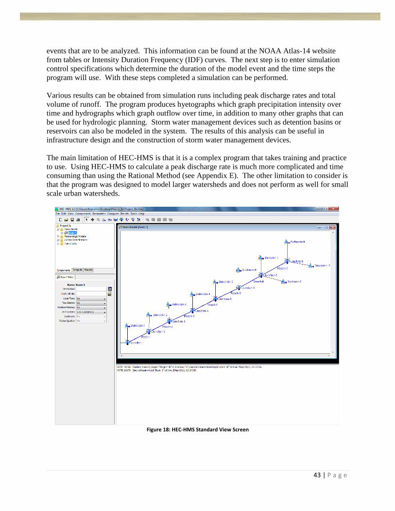
The main limitation of HEC-HMS is that it is a complex program that takes training and practice

to use. Using HEC-HMS to calculate a peak discharge rate is much more complicated and time

consuming than using the Rational Method (see Appendix E). The other limitation to consider is

that the program was designed to model larger watersheds and does not perform as well for small

scale urban watersheds.

Figure 18: HEC-HMS Standard View Screen

44 | P a g e

Appendix G

HEC-HMS Analysis – Pre-Development Watershed

Figure 19: HEC-HMS Watershed Model

Table 24: HEC-HMS Results, 5 year, 25 year, & 100 year storms

45 | P a g e

Figure 20: 5 year storm hydrograph



46 | P a g e

Appendix H

HEC-HMS Analysis – MCE Building Case Study

Figure 23: HEC-HMS Watershed Model for MCE Rooftop


47 | P a g e




48 | P a g e

Appendix I

HEC-HMS Analysis – Post-Development Watershed



49 | P a g e




50 | P a g e

Appendix J

HEC-HMS Analysis – Detention Basin


Table 27: HEC-HMS Results, 100-year storm

51 | P a g e

Figure 32: Detention Basin Storage Table and Volume Graph Vs. Time

Figure 33: Outlet Structure, Flow from 4 levels of Orifices

storm water runoff detention basin designco2.coe.utah.edu/cveen4410b/pdf/samplereport1.pdfstorm...

Documents