stochastic optimal control and the u.s financial debt crisis

Stochastic Optimal Controland the U.S. Financial Debt Crisis

Jerome L. Stein

Stochastic Optimal Controland the U.S. FinancialDebt Crisis

Jerome L. SteinDivision of Applied MathematicsBrown University Box FProvidence, RI, 02912, USA

ISBN 978-1-4614-3078-0 ISBN 978-1-4614-3079-7 (eBook)DOI 10.1007/978-1-4614-3079-7Springer New York Heidelberg Dordrecht London

Library of Congress Control Number: 2012932090

# Springer Science+Business Media New York 2012This work is subject to copyright. All rights are reserved by the Publisher, whether the whole or part ofthe material is concerned, specifically the rights of translation, reprinting, reuse of illustrations,recitation, broadcasting, reproduction on microfilms or in any other physical way, and transmission orinformation storage and retrieval, electronic adaptation, computer software, or by similar or dissimilarmethodology now known or hereafter developed. Exempted from this legal reservation are brief excerptsin connection with reviews or scholarly analysis or material supplied specifically for the purpose of beingentered and executed on a computer system, for exclusive use by the purchaser of the work. Duplicationof this publication or parts thereof is permitted only under the provisions of the Copyright Law of thePublisher’s location, in its current version, and permission for use must always be obtained fromSpringer. Permissions for use may be obtained through RightsLink at the Copyright Clearance Center.Violations are liable to prosecution under the respective Copyright Law.The use of general descriptive names, registered names, trademarks, service marks, etc. in thispublication does not imply, even in the absence of a specific statement, that such names are exemptfrom the relevant protective laws and regulations and therefore free for general use.While the advice and information in this book are believed to be true and accurate at the date ofpublication, neither the authors nor the editors nor the publisher can accept any legal responsibility forany errors or omissions that may be made. The publisher makes no warranty, express or implied, withrespect to the material contained herein.

Printed on acid-free paper

Springer is part of Springer Science+Business Media (www.springer.com)

In memory ofDAVID MORTON STEIN 1988–2008

Contents

1 Introduction . . . . . . . . . . . . . . . . . . . . . . . . . . . . . . . . . . . . . . . . . . . . . . . . . . . . . . . . . . . . . . . . . 1

1.1 The Subject and Contributions of This Book. . . . . . . . . . . . . . . . . . . . . . . . . . 4

References. . . . . . . . . . . . . . . . . . . . . . . . . . . . . . . . . . . . . . . . . . . . . . . . . . . . . . . . . . . . . . . . . . . 10

2 The Fed, IMF and Disregarded Warnings. . . . . . . . . . . . . . . . . . . . . . . . . . . . . . . 13

2.1 Greenspan’s Theme and the Fed. . . . . . . . . . . . . . . . . . . . . . . . . . . . . . . . . . . . . . 14

2.1.1 The Jackson Hole Consensus . . . . . . . . . . . . . . . . . . . . . . . . . . . . . . . . . 15

2.1.2 Desirable Leverage, Capital Requirements . . . . . . . . . . . . . . . . . . . 17

2.1.3 Market Anticipations of the Housing:

Mortgage Debt Crisis . . . . . . . . . . . . . . . . . . . . . . . . . . . . . . . . . . . . . . . . . 19

2.1.4 The Disregarded Warnings . . . . . . . . . . . . . . . . . . . . . . . . . . . . . . . . . . . 20

2.1.5 The Controversy Over Regulation

and Deregulation . . . . . . . . . . . . . . . . . . . . . . . . . . . . . . . . . . . . . . . . . . . . . . 22

2.1.6 The Failures of International Monetary

Fund Surveillance . . . . . . . . . . . . . . . . . . . . . . . . . . . . . . . . . . . . . . . . . . . . . 24

2.2 Conclusions . . . . . . . . . . . . . . . . . . . . . . . . . . . . . . . . . . . . . . . . . . . . . . . . . . . . . . . . . . . 25

References. . . . . . . . . . . . . . . . . . . . . . . . . . . . . . . . . . . . . . . . . . . . . . . . . . . . . . . . . . . . . . . . . . . 26

3 Failure of the Quants . . . . . . . . . . . . . . . . . . . . . . . . . . . . . . . . . . . . . . . . . . . . . . . . . . . . . . 29

3.1 Theme of This Chapter . . . . . . . . . . . . . . . . . . . . . . . . . . . . . . . . . . . . . . . . . . . . . . . 32

3.2 Leveraging . . . . . . . . . . . . . . . . . . . . . . . . . . . . . . . . . . . . . . . . . . . . . . . . . . . . . . . . . . . . 32

3.2.1 The Incredible Leverage of Atlas Capital Funding. . . . . . . . . . . 34

3.3 Structure of Derivatives Market, Rating Agencies

and Pricing of Derivatives . . . . . . . . . . . . . . . . . . . . . . . . . . . . . . . . . . . . . . . . . . . . 35

3.3.1 Pricing CDOs . . . . . . . . . . . . . . . . . . . . . . . . . . . . . . . . . . . . . . . . . . . . . . . . . 37

3.4 Major Premise of Economics/Finance: No Arbitrage

Principle (NAP) . . . . . . . . . . . . . . . . . . . . . . . . . . . . . . . . . . . . . . . . . . . . . . . . . . . . . . . 38

3.4.1 CAPM Model . . . . . . . . . . . . . . . . . . . . . . . . . . . . . . . . . . . . . . . . . . . . . . . . . 38

3.4.2 BSM Model . . . . . . . . . . . . . . . . . . . . . . . . . . . . . . . . . . . . . . . . . . . . . . . . . . . 39

3.4.3 The Efficient Market Hypothesis (EMH). . . . . . . . . . . . . . . . . . . . . 41

vii

3.4.4 The Quants and the Models. . . . . . . . . . . . . . . . . . . . . . . . . . . . . . . . . . . 42

3.4.5 The CAPM . . . . . . . . . . . . . . . . . . . . . . . . . . . . . . . . . . . . . . . . . . . . . . . . . . . . 43

3.4.6 Credit Default Swaps, EMH and the House

Price Index . . . . . . . . . . . . . . . . . . . . . . . . . . . . . . . . . . . . . . . . . . . . . . . . . . . . 44

3.5 When Has the Drift Changed? . . . . . . . . . . . . . . . . . . . . . . . . . . . . . . . . . . . . . . . . 47

3.6 Conclusion: Errors of the Quants . . . . . . . . . . . . . . . . . . . . . . . . . . . . . . . . . . . . . 50

References. . . . . . . . . . . . . . . . . . . . . . . . . . . . . . . . . . . . . . . . . . . . . . . . . . . . . . . . . . . . . . . . . . . 50

4 Philosophy of Stochastic Optimal Control Analysis (SOC) . . . . . . . . . . . . 53

4.1 Why Use Stochastic Optimal Control? . . . . . . . . . . . . . . . . . . . . . . . . . . . . . . . 53

4.2 Research Strategy . . . . . . . . . . . . . . . . . . . . . . . . . . . . . . . . . . . . . . . . . . . . . . . . . . . . . 56

4.3 Modeling the Uncertainty, the Stochastic Variables . . . . . . . . . . . . . . . . . 57

4.4 Criterion Function. . . . . . . . . . . . . . . . . . . . . . . . . . . . . . . . . . . . . . . . . . . . . . . . . . . . . 59

4.5 Methods of Solution of Stochastic Optimal Control Problem . . . . . . . 61

4.6 Loss of Expected Growth from Misspecification. . . . . . . . . . . . . . . . . . . . . 63

4.7 Insurance . . . . . . . . . . . . . . . . . . . . . . . . . . . . . . . . . . . . . . . . . . . . . . . . . . . . . . . . . . . . . . 65

4.7.1 Cramer-Lundberg . . . . . . . . . . . . . . . . . . . . . . . . . . . . . . . . . . . . . . . . . . . . . 65

4.7.2 Ruin Analysis . . . . . . . . . . . . . . . . . . . . . . . . . . . . . . . . . . . . . . . . . . . . . . . . . 66

4.7.3 The Stochastic Optimal Control Approach to Insurance . . . . . 67

4.8 The Endogenous Changing Distributions. . . . . . . . . . . . . . . . . . . . . . . . . . . . . 69

4.9 Mathematical Appendix . . . . . . . . . . . . . . . . . . . . . . . . . . . . . . . . . . . . . . . . . . . . . . 71

References. . . . . . . . . . . . . . . . . . . . . . . . . . . . . . . . . . . . . . . . . . . . . . . . . . . . . . . . . . . . . . . . . . . 73

5 Application of Stochastic Optimal Control (SOC)

to the US Financial Debt Crisis . . . . . . . . . . . . . . . . . . . . . . . . . . . . . . . . . . . . . . . . . . . 75

5.1 Introduction . . . . . . . . . . . . . . . . . . . . . . . . . . . . . . . . . . . . . . . . . . . . . . . . . . . . . . . . . . . 75

5.2 The Importance of the Housing/Mortgage Sector

to the Financial Sector . . . . . . . . . . . . . . . . . . . . . . . . . . . . . . . . . . . . . . . . . . . . . . . . 76

5.3 Characteristics of the Mortgage Market . . . . . . . . . . . . . . . . . . . . . . . . . . . . . . 77

5.4 The Stochastic Optimal Control Analysis . . . . . . . . . . . . . . . . . . . . . . . . . . . . 80

5.4.1 Model I . . . . . . . . . . . . . . . . . . . . . . . . . . . . . . . . . . . . . . . . . . . . . . . . . . . . . . . . 81

5.4.2 Model II . . . . . . . . . . . . . . . . . . . . . . . . . . . . . . . . . . . . . . . . . . . . . . . . . . . . . . . 83

5.5 Interpretation of Optimal Debt Ratio . . . . . . . . . . . . . . . . . . . . . . . . . . . . . . . . . 84

5.6 Empirical Measures of an Upper Bound

of the Optimal and Actual Debt Ratio. . . . . . . . . . . . . . . . . . . . . . . . . . . . . . . . 84

5.7 Early Warning Signals of the Crisis . . . . . . . . . . . . . . . . . . . . . . . . . . . . . . . . . . 86

5.8 The Market Delusion . . . . . . . . . . . . . . . . . . . . . . . . . . . . . . . . . . . . . . . . . . . . . . . . . 88

5.9 The Shadow Banking System: Leverage

and Financial Linkages . . . . . . . . . . . . . . . . . . . . . . . . . . . . . . . . . . . . . . . . . . . . . . . 89

5.9.1 Summary . . . . . . . . . . . . . . . . . . . . . . . . . . . . . . . . . . . . . . . . . . . . . . . . . . . . . . 94

References. . . . . . . . . . . . . . . . . . . . . . . . . . . . . . . . . . . . . . . . . . . . . . . . . . . . . . . . . . . . . . . . . . . 95

6 AIG in the Crisis . . . . . . . . . . . . . . . . . . . . . . . . . . . . . . . . . . . . . . . . . . . . . . . . . . . . . . . . . . . 97

6.1 Introduction . . . . . . . . . . . . . . . . . . . . . . . . . . . . . . . . . . . . . . . . . . . . . . . . . . . . . . . . . . . 97

6.2 AIG. . . . . . . . . . . . . . . . . . . . . . . . . . . . . . . . . . . . . . . . . . . . . . . . . . . . . . . . . . . . . . . . . . . . 98

6.3 The Economics and Actuarial Literature . . . . . . . . . . . . . . . . . . . . . . . . . . . 101

viii Contents

6.4 Stochastic Optimal Control (SOC) Approach

to Optimal Liabilities of a Large Insurer . . . . . . . . . . . . . . . . . . . . . . . . . . . 102

6.5 Mathematical Analysis. . . . . . . . . . . . . . . . . . . . . . . . . . . . . . . . . . . . . . . . . . . . . . 103

6.6 Solution for the Optimum Liability Ratio in General Model . . . . . . 105

6.7 Model Uncertainty and Optimal Liability Ratio . . . . . . . . . . . . . . . . . . . 106

6.8 Early Warning Signals . . . . . . . . . . . . . . . . . . . . . . . . . . . . . . . . . . . . . . . . . . . . . . 108

6.9 An Evaluation of the Bailout . . . . . . . . . . . . . . . . . . . . . . . . . . . . . . . . . . . . . . . 110

6.9.1 Government’s Justification for Rescue . . . . . . . . . . . . . . . . . . . . . 111

6.9.2 Panel’s Analysis of Options Available

to the Government and Decisions . . . . . . . . . . . . . . . . . . . . . . . . . . 112

6.10 Conclusions: Lessons to be Learned . . . . . . . . . . . . . . . . . . . . . . . . . . . . . . 114

References. . . . . . . . . . . . . . . . . . . . . . . . . . . . . . . . . . . . . . . . . . . . . . . . . . . . . . . . . . . . . . . . . 115

7 Crisis of the 1980s . . . . . . . . . . . . . . . . . . . . . . . . . . . . . . . . . . . . . . . . . . . . . . . . . . . . . . . 117

7.1 Introduction . . . . . . . . . . . . . . . . . . . . . . . . . . . . . . . . . . . . . . . . . . . . . . . . . . . . . . . . . 117

7.2 Stochastic Optimal Control (SOC) Analysis . . . . . . . . . . . . . . . . . . . . . . . 120

7.2.1 The Criterion Function. . . . . . . . . . . . . . . . . . . . . . . . . . . . . . . . . . . . . . 121

7.3 Dynamics of Net Worth. . . . . . . . . . . . . . . . . . . . . . . . . . . . . . . . . . . . . . . . . . . . . 121

7.4 The Stochastic Processes . . . . . . . . . . . . . . . . . . . . . . . . . . . . . . . . . . . . . . . . . . . 122

7.5 Solution and Interpretation of the Optimal Debt/Net Worth . . . . . . . 124

7.6 Basic Data . . . . . . . . . . . . . . . . . . . . . . . . . . . . . . . . . . . . . . . . . . . . . . . . . . . . . . . . . . . 125

7.7 Mean-Variance Interpretation. . . . . . . . . . . . . . . . . . . . . . . . . . . . . . . . . . . . . . . 126

7.8 Early Warning Signals . . . . . . . . . . . . . . . . . . . . . . . . . . . . . . . . . . . . . . . . . . . . . . 127

7.9 The S&L Crises . . . . . . . . . . . . . . . . . . . . . . . . . . . . . . . . . . . . . . . . . . . . . . . . . . . . . 129

References. . . . . . . . . . . . . . . . . . . . . . . . . . . . . . . . . . . . . . . . . . . . . . . . . . . . . . . . . . . . . . . . . 131

8 The Diversity of Debt Crises in Europe . . . . . . . . . . . . . . . . . . . . . . . . . . . . . . . . 133

8.1 Basic Statistics Related to the Origins of the Crises . . . . . . . . . . . . . . . 134

8.2 Crises in Ireland, Spain and Greece . . . . . . . . . . . . . . . . . . . . . . . . . . . . . . . . 136

8.2.1 Ireland . . . . . . . . . . . . . . . . . . . . . . . . . . . . . . . . . . . . . . . . . . . . . . . . . . . . . . . 136

8.2.2 Spain . . . . . . . . . . . . . . . . . . . . . . . . . . . . . . . . . . . . . . . . . . . . . . . . . . . . . . . . 137

8.2.3 Greece’s External Debt . . . . . . . . . . . . . . . . . . . . . . . . . . . . . . . . . . . . . 137

8.3 Role of the Capital Market . . . . . . . . . . . . . . . . . . . . . . . . . . . . . . . . . . . . . . . . . 138

8.4 Repercussions in Financial Markets . . . . . . . . . . . . . . . . . . . . . . . . . . . . . . . . 140

8.5 Origins of the External Debt Ratio . . . . . . . . . . . . . . . . . . . . . . . . . . . . . . . . . 140

8.5.1 Current Account/GDP and Net External Debt/GDP . . . . . . . 141

8.6 NATREX Model of External Debt

and Real Exchange Rate . . . . . . . . . . . . . . . . . . . . . . . . . . . . . . . . . . . . . . . . . . . . 143

8.6.1 Populist and Growth Scenarios . . . . . . . . . . . . . . . . . . . . . . . . . . . . . 146

8.7 NATREX Analysis of the European Situation . . . . . . . . . . . . . . . . . . . . . 149

8.8 Conclusions . . . . . . . . . . . . . . . . . . . . . . . . . . . . . . . . . . . . . . . . . . . . . . . . . . . . . . . . . 151

References. . . . . . . . . . . . . . . . . . . . . . . . . . . . . . . . . . . . . . . . . . . . . . . . . . . . . . . . . . . . . . . . . 154

Index . . . . . . . . . . . . . . . . . . . . . . . . . . . . . . . . . . . . . . . . . . . . . . . . . . . . . . . . . . . . . . . . . . . . . . . . . . 155

Contents ix

List of Figures

Fig. 2.1 Histogram and statistics of CAPGAINS ¼ Housing Price

Appreciation HPA, the change from previous four-quarter

appreciation of US housing prices, percent/year,

on horizontal axis. Frequency is on the vertical axis

(Source of data: Office of Federal Housing Price Oversight) . . . . . . 20

Fig. 2.2 PRICEINC ¼ Ratio of housing prices/disposable income.

DEBTSERVICE ¼ Debt service/disposable income. Both

variables are normalized (FRED data set of the Federal

Reserve Bank of St. Louis, Office of Federal Housing

Enterprise Oversight) . . . . . . . . . . . . . . . . . . . . . . . . . . . . . . . . . . . . . . . . . . . . . . . 21

Fig. 3.1 Ten-year treasury constant maturity rate . . . . . . . . . . . . . . . . . . . . . . . . . . . 30

Fig. 3.2 Three-month Treasury bill rate . . . . . . . . . . . . . . . . . . . . . . . . . . . . . . . . . . . . . 30

Fig. 3.3 Thirty-year conventional mortgage rate . . . . . . . . . . . . . . . . . . . . . . . . . . . . 31

Fig. 3.4 Histogram and statistics of CAPGAINS ¼ Housing Price

Appreciation HPA, the change from previous four-quarter

appreciation of US housing prices, percent/year, on horizontal

axis. Frequency is on the vertical axis. Period 1980q1–2007q4

(Source: Office of Federal Housing Price Oversight) . . . . . . . . . . . . . . 45

Fig. 3.5 Capital gains [P(t) – P(t�1)]/P(t�1) ¼ CAPGAIN;

DEBTRATIO ¼ household debt/disposable income

(Variables are normalized to a mean ¼ 0 and a standard

deviation ¼ 1) . . . . . . . . . . . . . . . . . . . . . . . . . . . . . . . . . . . . . . . . . . . . . . . . . . . . . . 46

Fig. 4.1 Expected growth of net worth, E [d ln X(t)] ¼ M[f(t)] � R[f(t)].

Variable f(t) ¼ debt/net worth or liabilities/surplus. . . . . . . . . . . . . . . . 62

Fig. 4.2 The change in expected growth equal to the difference

between the Mean M(f) and Risk R(f) in Fig. 4.1. . . . . . . . . . . . . . . . . . 63

Fig. 4.3 Optimum debt ratio and loss of expected net worth

from model mis-specification . . . . . . . . . . . . . . . . . . . . . . . . . . . . . . . . . . . . . . . 64

Fig. 4.4 Probability of ultimate ruin . . . . . . . . . . . . . . . . . . . . . . . . . . . . . . . . . . . . . . . . . 67

xi

Fig. 5.1 Household debt service payments as a percent of disposable

personal income, 1980–2011 (Source: Federal Reserve

of St. Louis, FRED, from Federal Reserve) . . . . . . . . . . . . . . . . . . . . . . . . 77

Fig. 5.2 Mortgage market bubble. Normalized variables. Appreciation

of single-family housing prices, CAPGAIN, 4q appreciation

of US Housing prices HPI, Office Federal Housing Enterprise

Oversight (OHEO); Household debt ratio DEBTRATIO ¼household financial obligations as a percent of disposable

income (Federal Reserve Bank of St. Louis, FRED,

Series FODSP. Sample 1980q1–2007q4). . . . . . . . . . . . . . . . . . . . . . . . . . . 78

Fig. 5.3 N[f(t)] ¼ DEBTSERVICE ¼ (household debt service payments

as percent of disposable income i(t)L(t)/Y(t) � mean)/standard

deviation. N[f**(t)] ¼ RENTPRICE ¼ (rental income/index

house price R(t)/P(t) � mean)/standard deviation

(Sources: FRED, OFHEO). . . . . . . . . . . . . . . . . . . . . . . . . . . . . . . . . . . . . . . . . . 86

Fig. 5.4 Early Warning Signal since 2004. C(t) ¼ EXCESS

DEBT ¼ N[f(t)] � N[f**(t)] ¼ DEBTSERVICE i(t)L(t)/Y

(t) � RENTRATIO R(t)/Y(t) . . . . . . . . . . . . . . . . . . . . . . . . . . . . . . . . . . . . . . . 87

Fig. 5.5 Capital gain CAPGAIN ¼ [P(t) � P(t � 1)]/P(t). House Price

Index, change over previous four quarters (e.g. 0.08 ¼ 8% pa)

(Federal Housing Finance Industry FHFA USA Indexes.

Sample: 1991q1–2011q1) . . . . . . . . . . . . . . . . . . . . . . . . . . . . . . . . . . . . . . . . . . . 88

Fig. 6.1 HPI/CAPGAIN Capital gains P tð Þ � P t� 1ð Þ½ �=P t� 1ð Þ,percent change in index of house price HPI,

sample 1991q1–2011q1 . . . . . . . . . . . . . . . . . . . . . . . . . . . . . . . . . . . . . . . . . . . . 107

Fig. 6.2 C tð Þ ¼ EXCESSDEBT, normalized excess debt ratio

of the mortgagors/households. . . . . . . . . . . . . . . . . . . . . . . . . . . . . . . . . . . . . . 109

Fig. 7.1 Ratio debt/equity (DEBTEQUITY), delinquency rate

(DELIQRATEFCS) of the agricultural sector. Normalized

variables. A normalized variable N(Z) is (Z-mean)/standard

deviation. Thus the mean is zero and the standard deviation

is unity (Source: Farm Security Administration, Economic

Research Service USDA) . . . . . . . . . . . . . . . . . . . . . . . . . . . . . . . . . . . . . . . . . . 118

Fig. 7.2 Agricultural bubble and collapse. Normalized variables.

INTVA ¼ interest payments/value added ¼ debt burden.

DELIQRATEFCS ¼ delinquency rate, farms security

administration, as a percent of loans. EQUITY ¼ assets �liabilities (Source: USDA (2002), Economic Research Service,

Agriculture Income and Finance, Farm Income and Balance

Sheet Indicators. Normalized variables) . . . . . . . . . . . . . . . . . . . . . . . . . . . 120

Fig. 7.3 Agriculture. GVACAP ¼ gross value added/capital ¼productivity of capital ¼ b(t), INTDEBT ¼ total interest

payments/debt ¼ r(t) . . . . . . . . . . . . . . . . . . . . . . . . . . . . . . . . . . . . . . . . . . . . . . . . 122

xii List of Figures

Fig. 7.4 RET1 ¼ GVACAP + GROWASSETS ¼ b(t),

INTDEB1 ¼ r(t) . . . . . . . . . . . . . . . . . . . . . . . . . . . . . . . . . . . . . . . . . . . . . . . . . . . . . 123

Fig. 7.5 Mean-variance interpretation of expected growth. . . . . . . . . . . . . . . . . 126

Fig. 7.6 Agriculture. DEBTNINC ¼ L/Y ¼ Debt/net income;

RETVAINTD ¼ GVACAP � INTDEBT ¼ (gross value added/

assets � interest rate). Normalized variable ¼ (variable � mean)/

standard deviation. . . . . . . . . . . . . . . . . . . . . . . . . . . . . . . . . . . . . . . . . . . . . . . . . . . . 128

Fig. 7.7 EXCESS DEBT ¼ DEBTNINC � RETVAINTD, normalized:

mean zero, standard deviation unity. Shaded period,

agricultural crisis . . . . . . . . . . . . . . . . . . . . . . . . . . . . . . . . . . . . . . . . . . . . . . . . . . . 129

Fig. 8.1 Interest rate spreads versus the Bund . . . . . . . . . . . . . . . . . . . . . . . . . . . . . . 139

Fig. 8.2 Saving less investment is SI and current account is CA.

Decline in social saving shifts SI from SI(0) to SI(1).

Real exchange rate appreciates to R(1) and current account

declines to A(1). The resulting rise in debt shifts CA

from CA(0) to CA(1). Real exchange rate depreciates

to R(2) and current account deficit rises to A(2) . . . . . . . . . . . . . . . . . . 147

Fig. 8.3 Populist scenario: initial R(0), F(0) at origin. Rise in social

consumption, increase demand for non-tradables generates

trajectory R(t) for the real exchange rate and F(t)

for the external debt. In the Growth scenario, the trajectories

for the real exchange rate and external debt trajectory

are reversed . . . . . . . . . . . . . . . . . . . . . . . . . . . . . . . . . . . . . . . . . . . . . . . . . . . . . . . . 148

Fig. 8.4 Euro area. Scatter diagram and regression line. Government

budget balance/GDP and current account/GDP

(Source: ECB Statistical Data Warehouse). . . . . . . . . . . . . . . . . . . . . . . . 152

Fig. 8.5 Euro-$US exchange rate . . . . . . . . . . . . . . . . . . . . . . . . . . . . . . . . . . . . . . . . . . . 154

List of Figures xiii

List of Tables

Table 2.1 Money, CPI, house price index, real GDP, percent

change from previous year. . . . . . . . . . . . . . . . . . . . . . . . . . . . . . . . . . . . . . . . 16

Table 3.1 Leverage of institutions . . . . . . . . . . . . . . . . . . . . . . . . . . . . . . . . . . . . . . . . . . . 33

Table 4.1 Alternative criteria/utility functions . . . . . . . . . . . . . . . . . . . . . . . . . . . . . . 60

Table 5.1 Banks’s aggregate portfolio. . . . . . . . . . . . . . . . . . . . . . . . . . . . . . . . . . . . . . . 76

Table 5.2 Contribution C(i) of factors to probability of delinquency

and defaults 2006, relative to mean for the period

2001–2006 . . . . . . . . . . . . . . . . . . . . . . . . . . . . . . . . . . . . . . . . . . . . . . . . . . . . . . . . 79

Table 6.1 AIG and the financial crisis, fall 2008. . . . . . . . . . . . . . . . . . . . . . . . . . . 100

Table 6.2 Tests for autocorrelation . . . . . . . . . . . . . . . . . . . . . . . . . . . . . . . . . . . . . . . . . 108

Table 6.3 Unit root tests . . . . . . . . . . . . . . . . . . . . . . . . . . . . . . . . . . . . . . . . . . . . . . . . . . . . 108

Table 6.4 Notional amount CDS outstanding $billions,

AIG-CDS rate 2001 h1–2010 h2 . . . . . . . . . . . . . . . . . . . . . . . . . . . . . . . . 110

Table 7.1 Histogram of debt/equity ratio (Source of data:

Economic Research Service USDA, Agricultural Income

and Finance Outlook/AIS-77/February 26, 2002) . . . . . . . . . . . . . . . 118

Table 7.2 Granger causality tests. Return ¼ capital gain plus

productivity of capital, against the debt/equity ratio . . . . . . . . . . . . 120

Table 7.3 Basic statistics: debt/equity ratio DEBTEQUITY ¼ L(t)/X(t),

gross value added/capital b(t) ¼ Y(t)/K(t) ¼ GVACP,

INTDEBT ¼ interest expenses/debt ¼ r(t) and

RETVAINTD1 ¼ GVACAP � INTDEBT ¼ Y(t)/K(t) � r(t) 125

Table 8.1 Government structural balance % GDP (SBGDP) . . . . . . . . . . . . . . 135

Table 8.2 Government net debt % GDP. . . . . . . . . . . . . . . . . . . . . . . . . . . . . . . . . . . . 135

Table 8.3 United States municipal rating distribution 1970–2000 . . . . . . . . . 139

Table 8.4 Banks and governments: debtor, creditor by country,

$billions . . . . . . . . . . . . . . . . . . . . . . . . . . . . . . . . . . . . . . . . . . . . . . . . . . . . . . . . . . 140

xv

Table 8.5 Current account/GDP . . . . . . . . . . . . . . . . . . . . . . . . . . . . . . . . . . . . . . . . . . . 141

Table 8.6 External debt position end 2009. . . . . . . . . . . . . . . . . . . . . . . . . . . . . . . . 141

Table 8.7 Residential property prices EU countries, annual % change,

new and existing houses . . . . . . . . . . . . . . . . . . . . . . . . . . . . . . . . . . . . . . . . 142

Table 8.8 NATREX dynamics of exchange rate and external debt:

two basic scenarios . . . . . . . . . . . . . . . . . . . . . . . . . . . . . . . . . . . . . . . . . . . . . 143

Table 8.9 Summary data 1998–2010 . . . . . . . . . . . . . . . . . . . . . . . . . . . . . . . . . . . . . . 150

Table 8.10 GDP deflator, percent change from year ago . . . . . . . . . . . . . . . . . . 151

xvi List of Tables

Chapter 1

Introduction

Abstract The theme of this book is that the application of Stochastic Optimal

Control (SOC) is very helpful in understanding and predicting debt crises.

The mathematical analysis is applied empirically to the financial debt crisis of

2008, the crises of the 1980s and concludes with an analysis of the European debt

crisis. I use SOC to derive a theoretically founded quantitative measure of an

optimal, and an excessive leverage/debt/risk that increases the probability of a

crisis. The optimal leverage balances risk against expected growth. The environ-

ment is stochastic: the capital gain, productivity of capital and interest rate are

stochastic variables, and for an insurance company, such as AIG, the claims are also

stochastic. I associate the housing price bubble with the growth of household debt.

A bubble is dangerous insofar as it induces a non-sustainable debt. This danger is

exacerbated insofar as a complex financial system is based upon it.

The Financial Crisis Inquiry Commission (FCIC) was created to examine the causes

of the financial and economic crisis in the US. It asked: How did it come to pass that

in 2008 our nation was forced to choose between two stark and painful alternatives –

either risk the total collapse of our financial system and economy or inject trillions

of taxpayer dollars into the financial system?

While the vulnerabilities that created the potential for crisis were years in the

making, the collapse of the housing bubble – fueled by low interest rates and

available credit, scant regulation and toxic mortgages – was the spark that ignited

a string of events, that led to a full-blown crisis in the fall of 2008. Trillions of

dollars of risky mortgages had become embedded throughout the financial system,

as mortgage related securities were packaged, repackaged, and sold to investors

around the world. When the bubble burst, hundreds of billions of dollars in losses in

mortgages and mortgage related securities shook markets and financial institutions

that had significant exposures to those mortgages and had borrowed heavily against

them. This happened, not just in the US but around the world.

J.L. Stein, Stochastic Optimal Control and the U.S. Financial Debt Crisis,DOI 10.1007/978-1-4614-3079-7_1, # Springer Science+Business Media New York 2012

1

Mortgage originators such as Countrywide sell packages of mortgages, household

debt to the major banks. The latter in turn structure the packages and tranche them

into senior, mezzanine and equity tranches. The income from the mortgages then

flows like a waterfall. The senior tranche has the first claim, the mezzanine has the

next and the equity tranche gets what, if anything is left. The illusion was that this

procedure diversified risk and that relatively riskless tranches could be constructed

from a melange of mortgages of dubious quality.

The securities firms finance the purchases from short term loans from banks

and money market funds, either repos secured by mortgages or commercial paper.

The securities firms then sell the collateralized debt obligations CDOs, the mezza-

nine and equity tranches as packages to international investors, investment banks

such as Merrill Lynch, Citi-group, Goldman-Sachs and hedge funds. These

purchasers finance the purchases by short term bank borrowing. Securities firms

and hedge funds may buy Credit Default Swaps (CDS) from companies such as

AIG as insurance against declines in the values of the CDOs. If the mortgagors are

unable to service their debts – the income from the mortgages declines – the

repercussions are felt all along the line. This is a systemic risk that was ignored.

Despite the post crisis expressed view of many on Wall St. and in Washington

that the crisis could not have been foreseen or avoided, the FCIC argued there were

warning signs. The tragedy was that Washington and Wall St. ignored the flow

of toxic mortgages and could have set prudent mortgage-lending standards.

The Federal Reserve was the one entity empowered to do so and did not.

Regulators had ample power to protect the financial system and they chose not to

use it. SEC could have required more capital and halted risky practices at the big

investment banks. It did not. The Federal Reserve Bank of N.Y. (FRNY) and other

regulators could have clamped down on Citigroup’s excesses in the run up to the

crisis. They did not. The dramatic failures of corporate governance and risk

management at many systemically important financial institutions were a key

cause of this crisis.

Many financial institutions as well as too many households borrowed to the hilt,

leaving them vulnerable to financial distress or ruin if the value of their investments

declined even moderately. As of 2007 the five major investment banks – Bear

Stearns, Goldman Sachs, Lehman Brothers, Merrill Lynch and Morgan Stanley

were operating with thin layers of capital – leverage ratios as high as 40:1. Less than

a 3% drop in asset values would wipe out the firm.

A key institution in the financial crisis was AIG. At its peak it was one of the

largest and most successful companies in the world. AIG’s senior management

ignored the terms and risks of the company’s $79 billion derivatives exposure to

mortgage related securities. The financial crisis put its credit rating under pressure,

because AIG lacked the liquidity to meet collateral demands. In a matter of months

AIG’s worldwide empire collapsed.

The government was ill prepared for the crisis and its inconsistent response added

to the uncertainty and panic in financial markets. It had no comprehensive and

strategic plan for containment, because it lacked a full understanding of the risks

and interconnection in the financial markets.

2 1 Introduction

Prior to the crisis, it appeared to the academic world, financial institutions,

investors, and regulators alike that risk had been conquered. The capital asset

pricing model (CAPM) developed by Markowitz, Sharpe and Lintner explained

the pricing of securities and how to manage risk. The options pricing model of

Black, Scholes and Merton was used to construct financial derivatives with desired

risk-expected returns combinations. Using these techniques, physicists,

mathematicians and computer scientists – the Quants – were attracted to Wall St.

to use good mathematics to manufacture financial derivatives.

Investors held highly rated securities they thought were sure to perform; the

banks thought that they had taken the riskiest loans off their books; and regulators

saw firmsmaking profits and borrowing costs reduced. But each step in themortgage

securitization pipeline depended upon the next step to keep demand going.

The Fed and the IMF, who employed large numbers of PhD’s in economics,

were charged with surveillance of financial markets. The Fund surveillance reports

reflect the state of the art – the quality of the models – in the economics profession.

There was no fear of a financial crisis because the prevailing view was that they

were the consequences of monetary excesses. The pre crisis period was the Great

Moderation: moderate money growth and inflation and satisfactory real growth.

Hence no cause to worry.

The Independent Evaluation Office (IEO) of the IMF assessed the performance

of the IMF surveillance in the run up to the global financial crisis. It found that the

IMF provided few clear warnings about the risks and vulnerabilities associated with

the impending crisis before its outbreak in the US and elsewhere. For example, in

spite of the fact that Iceland’s banking sector had grown from about 100% of GDP in

2003 to almost 1,000% in 2007, the Fund did not recognize that this was a vulner-

ability that needed to be addressed urgently. Just before the crisis the IMF wrote

that Iceland’s medium term prospects remained enviable. They did not consider that

Iceland’s high leverage posed a risk to the financial system. The banner message was

one of continued optimism after more than a decade of benign economic conditions

and low macroeconomic volatility.

The IMF and the economics profession missed key elements that underlay the

developing crisis. There was a “group think” mentality: this homogeneous group

of economists in the Fund only considered issues within the prevailing paradigm in

economics and there were no significant challenges to this point of view. The key

assumption was that market discipline and self-regulation would be sufficient to

stave off serious problems in financial institutions.

Neither the Fed nor the IMF discussed, until the crisis had already erupted, the

deteriorating lending standards for mortgage financing, or adequately assessed the

risks and impact of a major housing price correction on financial institutions. In fact

the IMF praised the US for its light touch regulation and supervision that ultimately

contributed to the problems of the financial system. Moreover, the IMF recom-

mended that other advanced countries follow the US/UK approach. The Fund did

not see the similarities between developments in the US and UK and the experience

of other advanced economies and emerging markets that had previously faced

financial crises.

1 Introduction 3

1.1 The Subject and Contributions of This Book

The Dodd-Frank (D-F) bill establishes the Financial Services Oversight Council.

The bill authorizes the Federal Reserve Board to act as agent for the Council to

monitor the financial services marketplace to identify potential threats to the

stability of the US financial system and to identify global trends and developments

that could pose systemic risks to the stability of the US economy and to other

economies. Neither the Fed nor the IMF, who based their analysis upon the

dominant economic paradigm, has demonstrated its ability to fulfill these

requirements. The techniques used by the Quants and rating agencies, based upon

the dominant stochastic models, proved inadequate.

The four major studies of the US financial crisis are: Greenspan’s Retrospective(2010); the Financial Crisis Inquiry Commission Report (FCIC 2011); Congres-

sional Oversight Panel (COP 2010) The AIG Rescue, Its Impact on Markets and the

Government’s Exit Strategy; Congressional Oversight Panel (COP 2009), SpecialReport on Regulatory Reform. There is a large economics literature on the crisis in

conference volumes and journals. They cover the same ground as the four major

studies above and are primarily descriptive. Several discuss regulation and capital

requirements but their recommendations are not based upon an optimizing frame-

work. They do not provide analytical tools to answer the questions: (Q1) What is a

theoretically founded quantitative measure of an optimal leverage? (Q2) What is an

excessive risk that increases the probability of a crisis? (Q3) What is the expla-

natory power of the analysis?

The theme of this book is that the application of Stochastic Optimal Control is

very helpful in understanding and predicting debt crises and in evaluating risk

management. I associate the housing price bubble with the growth of household

debt. A bubble is dangerous insofar as it induces a non-sustainable debt.This danger is exacerbated insofar as a complex financial system is based upon it.

My analysis uses Stochastic Optimal Control (SOC) to answer questions (Q1)–(Q3)

above. The optimal capital requirement/leverage balances risk against expected

growth. The environment is stochastic: the capital gain, productivity of capital and

interest rate are stochastic variables, and for an insurance company, such as AIG,

the claims are also stochastic. In this manner the SOC approach developed in this

book satisfies the requirements of the D-F bill described above.

There is a large economics literature that describes the crisis. There is a large

mathematics literature on stochastic optimal control. My book synthesizes the two

approaches. It is aimed at economists and mathematicians who are interested in

understanding how SOC based techniques could have been useful in providingearly warning signals of the recent crises, and at those interested in risk manage-

ment. Key issues below are the subjects of the subsequent chapters and constitute

the theme and contribution of this book.

Chapter 2 explains why the financial markets, and the Fed/IMF/economics

profession, failed to anticipate the mortgage/housing and financial crisis and the

vulnerability of AIG. They used inappropriate models and hence incorrectly

4 1 Introduction

evaluated risk and the probability of bankruptcy/ruin. The crucial ultimate variable

is the household debt, the mortgage debt. The rest of the financial system rested

upon the ability of the mortgagors to service their debts. Systemic risk describes theeffects of the failure of the mortgagors to service their debts upon the financial

structure. The leverage of the financial system transmitted the housing market

shock into a collapse of the financial system.

A bubble is in effect a large positive “excess, unsustainable debt”. Detection of abubble corresponds to the detection of an “excess debt”. The aim of this book is to

derive an optimal debt/net worth ratio and excess debt ratio. The latter is equal to the

difference between the actual and the optimal debt. The fundamentals are reflected

in the optimal debt. The housing price bubble, its subsequent collapse, and the

financial crisis were not predicted by either the market, the Fed, the IMF or

regulators in the years leading to the crisis. Moreover, the Fed and Treasury rejected

the warnings based upon publicly available information, and successfully advocated

deregulation of Over The Counter (OTC)markets. As a result, transparency of prices

was reduced, risk was concentrated in a few major financial institutions, and high

leverage was induced. These were basic ingredients for the subsequent crisis.

The Fed, the IMF and Treasury lacked adequate tools, which might have

indicated that asset values were vastly out of line with fundamentals. The Fed

and the Fund were not searching for such tools because they did not believe that

they could or should look for misaligned asset values or excess debt, despite

warnings from Shiller, some people in the financial industry, the GAO, state bank

regulators and FDIC. The Fed was blind-sided by the Efficient Market Hypothesis

(EMH), that current prices reveal all publicly available information. One cannot

second – guess the market. There cannot be an ex-ante misalignment. Bubbles exist

only in retrospect. The Jackson Hole Consensus gave them great comfort in

adopting a hands off position by claiming that “As long as money and credit remain

broadly controlled, the scope for financing unsustainable runs in asset prices should

also remain limited. . ..numerous empirical studies have shown that almost all asset

price bubbles have been accompanied, if not preceded by strong growth of credit

and or money”. Since the period preceding the crisis was the Great Moderation,

there was no need to worry.

So it was not just a lack of appropriate tools that undid the Fed; it was a complete

lack of appreciation of what its role should be in heading off an economic catas-

trophe. There are two separate but related questions: Are identification and contain-

ment of a financial bubble legitimate activity of the Fed, and if they are, what are the

best tools to carry out this analysis.

Former chairman of the Federal Reserve Board Alan Greenspan has great

knowledge of financial markets. I think that his behavior may be explained ratio-

nally. First he understands that the function of financial markets is to channel saving

into investment in the optimal way to promote growth. Second, like most of the

economics profession, he or his staff accepted the generality of the First Theorem ofWelfare Economics. This theorem states that a Competitive Equilibrium is a Pareto

Optimum. The implication is that “market regulation” is superior to regulation by

bureaucrats, politicians. Do not try to second guess the markets.

1.1 The Subject and Contributions of This Book 5

The belief in the generality of the First Theorem of Welfare Economicsmay have

provided a basis for Greenspan’s position. The Theorem does not hold in financial

markets for several reasons. First, financial assets are not arguments in the utility

function of households so that it makes little sense to say that the relative asset

prices equal marginal rates of substitution. There is no tangency of indifference

curves with the price line. Second, the assumption of atomistic agents operating in

perfectly competitive markets with full information and stable preferences is wildly

unrealistic. The Efficient Market Hypothesis EMH was a major foundation of

Greenspan’s view and that of the finance profession.

Chapter 3 considers the role of the “Quants”/mathematical finance. They are the

physicists, mathematicians and computer scientists who were attracted to Wall St.

The mathematics per se was not at fault in the crisis, but the finance models used

were inadequate and grossly underestimated risk.

The finance literature was based upon the Efficient Market Hypothesis (EMH),

the Black-Scholes-Merton (BSM) options price model and the CAPM. The EMH

claims that asset markets are, to a good approximation, informationally efficient.

Market prices contain most information about fundamental value. Prices of traded

assets already reflect all publicly available information. The CAPM provides a good

measure of risk. Assets can only earn high average returns if they have high betas.

Average returns are driven by beta because beta reflects the extent that the addition

of a small quantity of the asset to a diversified portfolio adds to the volatility of the

portfolio. On the basis of the EMH and CAPM, Greenspan, the Fed and the finance

profession believed that markets would be self-regulating through the activities

of analysts and investors. Government intervention weakens the more effective

private regulation.

Securitization/tranching, the CDOs and derivatives of derivatives produced an

environment where the EMH/CAPM lost relevance. These bundles of many mort-

gage based securities seemed to tailor risk for different investors. Securitization/

tranching gave the illusion that one could practically eliminate risk from risky

assets and led to very high leverage. Ratings of the tranches were not based upon the

quality of the underlying mortgages. They were all in the same bundle. The rating

depended upon who got paid first in the stack of loans. The key question was how to

rate and price the tranches. The issue concerned the correlation of the tranches. If a

pool of loans started experiencing difficulties, and a certain percent of them

defaulted, what would be the impact upon each tranche? The “apples in the basket

model” assumed that they were like apples in a basket with a certain fraction of

them being rotten. If one apple is rotten, it says nothing about whether the next

apple chosen is rotten. Another very different one is “the slice of bread in the loaf”

model. In that model if a slice (tranche) of bread is moldy, what is the probability

that the next slice – or the rest of the loaf – is moldy? The Quants falsely assumed

independence of tranches and assumed that they could tranche packages of “toxic

assets” to produce a riskless tranche.

The Quants ignored how the interactions of the firms affected the return on the

CDOs. The collapse of one group led to severe losses in groups before and after it in

6 1 Introduction

the chain. For example, the collapse of AIG affected the prices of “safe” as well as

of risky assets. They based their estimates of risk upon the recent non-sustainable

distribution of housing prices. They ignored the “no free lunch” constraint that

capital gains cannot consistently exceed the mean interest rate. Most important,

they ignored publicly available information concerning systemic risk. Their models

ignored the systemic risk that the mortgagors would be unable to repay debt.

The prices of many of the securities traded were opaque and estimated using

arbitrary computer models. Hence the values of assets and liabilities on balance

were not reflective of what they could fetch if sold.

Chapter 4 discusses the philosophy of the stochastic optimal control (SOC)

techniques used in later Chaps. 5, 6 and 7. Modeling is crucial in economics and

finance. Fisher Black, who developed the equation for options modeling, argued

that given the models’ limitations, “the right way to engage with a model is, like a

fiction reader or a really great pretender, is to suspend disbelief and push it as far as

possible. . . But then, when you’ve done modeling, you must remind yourself that

. . . although God’s world can be divined by principles, humanity prefers to remain

mysterious. Catastrophes strike when people allow theories to take on a life of their

own and hubris evolves into idolatry.”(quoted in Derman).

The net worth of the real estate sector in Chap. 5, and of AIG on Chap. 6, evolve

dynamically. In the first case, debt is incurred in period t to purchase assets

whose return is uncertain, and must be repaid in period t + 1 at an uncertain interest

rate. In the second case, insurance is sold in period t and the claims in period t + 1 are

uncertain. What is the optimal debt in the first case and what are the optimal

insurance liabilities in the second case?

I discuss the strengths and limitations of alternative criterion functions, what

should the firm or industry maximize? How should risk aversion be taken into

account? Then I discuss the modeling of reasonable stochastic processes of the

uncertain variables. Given the criterion function, each stochastic process implies a

different quantitative, but similar qualitative, optimum debt/net worth or insurance

liabilities/net worth. Using SOC I derive quantitative measures of an optimal and

an excessive leverage, an excessive risk that increases the probability of a crisis.

The optimal capital requirement or leverage balances risk against expected growth

and return. The implications of the analysis are described graphically in the text and

proved mathematically in an appendix. As the actual debt ratio exceeds the optimal

ratio the expected growth declines and the risk rises. Thereby the probability of a

debt crisis is directly related to the excess debt, the actual less optimal. A bubble is

an unsustainable excess debt. The second part of the chapter discusses the models

used in the insurance, or actuarial literature, concerning the probability of ruin.

They are then compared with the SOC approach.

Chapter 5 applies this SOC analysis to the US financial crisis. I discuss the

importance of the housing/real estate sector to the financial sector, and the

characteristics of the mortgage market. Then two models of the stochastic process

on the capital gain and interest rate are presented. Each implies a different value of

the optimal debt/net worth. In order to do an empirical analysis, I derive an upper


bound of the optimal debt ratio, based upon the alternative models, to derive a

measure the excess debt: actual less the upper bound of the optimal ratio.

The derived excess debt is shown to be an early warning signal (EWS) of the debt

crisis as early as 2004.

Finally, the shadow banking system is discussed. The financial crisis was

precipitated by the mortgage crisis for several reasons. First, a whole structure of

financial derivatives was based upon the ultimate debtors – the mortgagors. Insofar

as the mortgagors were unable to service their debts, the values of the derivatives

fell. Second, the financial intermediaries whose assets and liabilities were based

upon the value of derivatives were very highly leveraged. Changes in the values of

their net worth were large multiples of changes in asset values. Third, the financial

intermediaries were closely linked – the assets of one group were liabilities of

another. A cascade was precipitated by the mortgage defaults. Since the “Quants”

were following the same rules, the markets could not be liquid. In this manner, the

mortgage debt crisis turned into a financial crisis.

Chapter 6 concerns insurance, the AIG case. First, I describe what happened to

AIG in the 2007–2008 crisis. Then I evaluate the actuarial literature on optimal risk

and capital requirements for insurers – Cramer-Lundeberg, ruin problems. I explain

how SOC is a much more powerful tool of analysis. The stochastic optimal (SOC)

approach’s components are: the criterion function, the stochastic differential

equations, and the stochastic processes. The solution for the optimal insurance

liability/claims requirement on the basis of SOC follows. The chapter concludes

with an evaluation of the government bailout.

AIG seriously underestimated risk because it ignored the negative correlation

between the capital gain on insured assets and the liabilities/claims on AIG. The

CDS claims grew when the value of the insured obligations CDO declined. This set

off collateral requirements, and the stability of AIG was undermined. The chapter

concludes with an evaluation of the government bailout.

Chapter 7 concerns the agricultural crisis of the 1980s and the S&L crisis in the

1980s. I explain that these crises had many features in common, but were localized.

The crisis of 2007–2008 shared the common elements of the earlier two but was

more pervasive and severe due to the financial structure that was based upon the

housing/mortgage sector. This focus is upon the crisis of the 1980s, in particular

the agriculture crisis. The policy issues are: How should creditors, banks and bank

regulators evaluate and monitor risk of an excessive debt that significantly increases

the probability of default? I show how the same techniques of stochastic optimal

control used in Chaps. 5 and 6 are useful in providing early warning signals for

the agricultural crisis. In the concluding part I compare the S&L crisis to the

agricultural crisis.

Chapter 8 goes beyond the US financial crisis of 2008 and explains the inter

country differences in the debt crisis in Europe. This subject is timely and I cannot

ignore it. The external debts of the European countries are at the core of the current

European crises. Generally, the crises are attributed to government budget deficits in

excess of the values stated in the Stability and Growth Pact (SGP)/Maastricht treaty.

8 1 Introduction

Proposals for reform generally involve increasing the powers of the European Union

tomonitor fiscal policies of the national governments and increasing bank regulation.

I explain: (a) to what extent the crises in the different countries were due to

government budget deficits/government dissaving or to the private investment less

private saving, (b) what is the mechanism whereby the actions of the public and

private sectors lead to an unsustainable debt burden, defined as the ratio of debt

service/GDP. The Stability and Growth Pact/Maastricht Treaty and the European

Union focused upon rules concerning government debt ratios and deficit ratios.

They ignored the problem of “excessive” external debt ratios in the entire economy

that led to a crisis in the financial markets.

The techniques of analysis in this chapter differ from those in the previous

chapters. In the previous chapters the debt ratio was a control variable. Using

stochastic optimal control, I derived optimal debt ratios. This is normative economics.

Chapter 8 is concerned with positive economics. The external debt ratio is not a

control variable, but is an endogenous variable that is determined by “fundamentals”

in a dynamic manner. The “fundamentals” are determined by the actions of both the

public and the private sectors. I explain this by drawing upon the Natural Real

Exchange Rate NATREX model (Stein 2006) of the equilibrium real exchange rate

and external debt – the endogenous variables.

In this book, I do not discuss policy issues: regulation and reform. A Dissenting

Statement by Wallison, in the Financial Crisis Inquiry Commission Report is:

“The question that I have been most frequently asked about the Financial Crisis

Inquiry Commission [FCIC] is why Congress bothered to authorize it all. Without

waiting for the Commission’s insights into the causes of the financial crisis,

Congress passed and the President signed the Dodd-Frank Act (DFA), [with] far

reaching and highly consequential regulatory legislation.” The focus of my book is

positive economics, and I avoid the political, normative, divisive and sociological

aspects that regulation entails.

The history of this book reflects my debts to many people. When I retired from

the economics department I was invited in 1997 by the Division of Applied

Mathematics (DAM) to be a visiting professor/research. I had worked with Ettore

Infante (DAM) for a decade in the 1960–1970s applying deterministic optimal

control to economic problems in feedback form. I felt that I was returning home.

Wendell Fleming and I started to discuss how and to what extent the techniques of

stochastic optimal control can be useful in economics. Wendell is renowned for his

contributions to pure and applied mathematics, and his book with Ray Rishel is

essential reading. We decided that the debt crises would be an appropriate subject

of interdisciplinary research. Thus I had to learn the mathematics literature using

dynamic programming to determine what is an optimal trajectory of the debt. Our

regular meetings resulted in our first article, Fleming and Stein (2004) in the Journal

of Banking and Finance. I was invited to give a paper at the AMS-IMS-SIAM

Research Conference in Mathematical Finance (2003), where I explained how one

can successfully apply the techniques of the H-J-B equation to the crises of the

1980s. This was my first contact with the elite in the profession. They were masters


of the techniques but were unaware of what one could do with them for real world

problems in economics. I edited and contributed to a special issue of Australian

Economic Papers “Stochastic Models in Economics and Finance” (2005). I was

then invited to give a paper at a mathematics conference at the University of

Wisconsin/Milwaukee applying the mathematical techniques to the US balance

of payments. There I got to know Ray Rishel, who has been most helpful to me.

I then edited and contributed to a Special Issue of the Journal of Banking and

Finance “Intertemporal Optimization in a Stochastic Environment” (2007).

EUROPT invited me twice, once to Prague and once to Lithuania, to give

keynote addresses about different aspects of my work. I was the only economist

on the programs, the rest were mathematicians and O/R experts.

The next phase consisted of writing a series of articles aimed at economists

under the rubric “Greenspan, Dodd-Frank and Stochastic Optimal Control”.

My aim was to explain how the failures of the Fed could have been avoided had

the Fed used my techniques.

I felt that I had done all that I could to bring my work to the attention of the

various professions. However, the Springer-Science editor Brian Foster wrote that

there are many books on stochastic control and many descriptive books on the

crisis, but none applied the techniques of SOC to the crises. Would I consider doing

a book on the subject? Springer published Fleming-Rishel, so my book would be

a nice complement.

It was unclear tomewho could be the readership? I consulted Seth Stein, the author

of Disaster Deferred on earthquake prediction. His advice was to write the book that

I want to write and not write it with any specific constituency in mind. He suggested

how I should present the mathematics in a way that both mathematicians and

economists would benefit. He has been a constant source of excellent advice.

I had the good fortune to receive the advice and criticism from several sources.

Peter Clark, Serge Rey, Karlhans Sauernheimer, Christoph Fischer and Carl

D’Adda have been my economics critics. They have suggested many changes in

points of view. Wendell Fleming and Ray Rishel have been my mathematics critics.

Ren Cheng (Fidelity Investments) and Robert Selvaggio (Rutter Associates) have

my consultants on what has been going on in the finance industry.

References

Congressional Oversight Panel, COP. 2009. “Special Report on Regulatory Reform”. Affairs,

New York.

Congressional Oversight Panel. 2010. The AIG rescue, its impact on markets and the government’sexit strategy. Washington, DC: U.S. G.P.O.

Derman, Emanuel. 2004. My life as a quant. New York: Wiley.

Financial Crisis Inquiry Report. 2011. FCIC, Public Affairs, N.Y.

10 1 Introduction

Fleming, Wendell H., and Jerome L. Stein. 2004. Stochastic optimal control, international finance

and debt. Journal of Banking and Finance 28: 979–996.Greenspan, Alan. 2010. The Crisis, Brookings papers on Economic Activity.

International Monetary Fund, Independent Evaluation Office. 2011. IMF performance in therun-up to the financial and economic crisis. Washington, DC: International Monetary Fund.

Stein, Jerome L. 2006. Stochastic optimal control, international finance and debt crises.New York: Oxford University Press.

Stein, Seth. 2010. Disaster deferred. New York: Columbia University Press.

References 11

Chapter 2

The Fed, IMF and Disregarded Warnings

Abstract The Fed, the IMF and Treasury lacked adequate tools, which might

have indicated that asset values were vastly out of line with fundamentals. The Fed

and the Fund were not searching for such tools because they did not believe that they

could or should look for misaligned asset values or excess debt, The Fed was blind-

sided by the EfficientMarketHypothesis (EMH), that current prices reveal all publicly

available information. One cannot second- guess the market. There cannot be an ex-

antemisalignment. Bubbles exist only in retrospect. The JacksonHoleConsensus gave

themgreat comfort in adopting a hands off positionbyclaiming that “As longasmoney

and credit remain broadly controlled, the scope for financing unsustainable runs in

asset prices should also remain limited. . ..numerous empirical studies have shown that

almost all asset pricebubbles havebeen accompanied, if not precededby stronggrowth

of credit and or money”. Since the period preceding the crisis was the Great

Moderation, there was no need to worry.

The theme of this chapter is to explain why the financial markets, the Fed, IMF, and

economics profession failed to anticipate the mortgage housing and financial crisis.

I associate a bubble, such as in housing prices or agricultural prices, with an“excess debt”. There were debt crises in the 1980s – the agricultural crisis and the

S&L crisis. They were very similar to the 2007–2008 financial crisis. The big

difference was that the agricultural crisis was localized. On the other hand the

housing sector and financial sectors were highly interrelated and leveraged. The Fed

lacked a theoretical model with explanatory power to evaluate systemic risk and theprobability of bankruptcy/ruin resulting from debt. The Fed and then Chairman

Greenspan did not understand how to measure what is an “excessive” debt or

leverage or unduly low capital requirement that will raise the probability of a crisis.

This chapter is organized as follows. First I discuss the Fed’s and Greenspan’s

views. Second, I discuss the market anticipations, disregarded warnings and why the

financial market failed to anticipate the crisis. Third, I discuss the controversy over

deregulation. Fourth, I discuss the failures of the IMF and economics profession.


13

2.1 Greenspan’s Theme and the Fed

Prior to the subprime crisis of 2007, there was a false sense of safety in financial

markets. Alan Greenspan (2004a) said “. . .the surge in mortgage refinancings likely

improved rather than worsened the financial condition of the average homeowner”.

Moreover “Overall, the household sector seems to be in good shape, and much of

the apparent increase in the household sector’s debt ratios in the past decade reflects

factors that do not suggest increasing household financial stress”.

The market and the Fed did not consider these mortgages to be very risky.

In February 2004, a few months before the Fed formally ended a run of interest rate

cuts, Greenspan (2004b) said that “. . .improvements in lending practices driven by

information technology have enabled lenders to reach out to households with

previously unrecognized borrowing capacity. This extension of lending has

increased overall household debt but has probably not meaningfully increased the

number of households with already overextended debt.” By 2007, a measure of risk,

the yield spread (CCC bonds – 10 year US Treasury) fell to a record low.

Fed Chairman Ben Bernanke said (2005) in his testimony before Congress’s

Joint Economic Committee that US house prices have risen by nearly 25% over the

past 2 years. However, these increases “largely reflect strong economic

fundamentals” such as strong growth in jobs, incomes and the number of new

households”.

The failure to realize that there was an unsustainable bubble that would damage

the world economy was pervasive. As late as April 2007, the IMF noted that

“. . .global economic risks declined since. . .September 2006. . .The overall US

economy is holding up well . . .[and] the signs elsewhere are very encouraging.”

The venerated credit rating agencies bestowed credit ratings that implied AAA

smooth sailing for many a highly toxic derivative product.

In 2008 Greenspan said “Those of us who have looked to the self-interest of

lending institutions to protect stockholders’ equity, myself included, are in a state of

disbelief”. In his retrospective he asks: could the breakdown have been prevented?

The Fed was lulled into complacency about a bursting of the bubble and its

aftermath because of recent history. First, they anticipated that the decline in

home prices would be gradual. Second, there were only modestly negative effects

of the 1987 stock market crash. The injections of Fed liquidity apparently helped

stabilize the economy.

Greenspan’s paper (2010) presents his retrospective view of the crisis. His theme

has several parts. First, the decline and convergence of world real long term interest

rates – not Federal Reserve monetary policy – led to significant housing price

appreciation, a housing price bubble. This bubble was leveraged by debt. There

was a heavy securitization of subprimemortgages. In the years leading to the current

crisis, financial intermediation tried to function on too thin layer of capital – high

leverage – owing to a misreading of the degree of risk embodied in ever more

complex financial products and markets. Second, when the bubble unraveled, the

leveraging set off a series of defaults. Third, the breakdown of the bubble was

14 2 The Fed, IMF and Disregarded Warnings

unpredictable and inevitable, given the “excessive” leverage – or unduly low capital

– of the financial intermediaries. Fourth, the lesson for the future is that is imperative

that there be an increase in regulatory capital and liquidity requirements by banks.

2.1.1 The Jackson Hole Consensus

Otmar Issing (former chief economist for the European Central bank, ECB)

discussed the Lessons to be learned by Central banks from the recent financial

crisis. The main thrust of his argument was a criticism of the Jackson Hole

Consensus (JHC 2005) for the relation between asset price bubbles and the conduct

of monetary policy.

During the boom years, abundant liquidity and low interest rates led to a

situation of excessive risk taking and asset price bubbles. The JHC has been the

prevailing regulatory approach taken by the Fed. It is based upon three principles.

Central banks: (1) should not target asset prices, (2) should not try to prick an asset

price bubble, (3) should follow a “mopping up” strategy after the bubble bursts by

injecting enough liquidity to avoid serious effects upon the real economy.

A justification for this policy was seen in the period 2000–2002 with the collapse

of the dot.com bubble. The “mopping up” seemed to work well and there were no

serious effects upon the real economy from following the JHC.

Issing objects to the JHC because it constitutes an asymmetric approach. When

asset prices rise without inflationary effects measured by the CPI, this is deemed

irrelevant for monetary policy. But when the bubble bursts, central banks must

come to the rescue. This, he argues, produces a moral hazard. He notes that

although the JHC strategy worked well in the 2000–2002 period it should not

have justified the assumption that it would work afterwards in other cases.

The JHC strategy certainly did not work in the 2007–2008 crisis that was precipit-

ated by the bursting of the housing price bubble. He wrote: “Did we really need a

crisis that brought the world to the brink of a financial meltdown to learn that the

philosophy which was at the time seen as state of the art was in fact dangerously

flawed?. . .we must conduct a thorough discussion as to appropriate strategy of

central banks with respect to asset prices.”

Issing favors giving the central banks a mandate for macro-prudential supervi-

sion. The ECB should be responsible for identifying macroeconomic imbalances

and for issuing warnings and recommendations addressed to national policy

makers. The “solution” proposed is one that monitors closely monetary and credit

developments as the potential driving forces for consumer price inflation in the

medium to short run. “As long as money and credit remain broadly controlled,

the scope for financing unsustainable runs in asset prices should also remain

limited.” He notes: “numerous empirical studies have shown that almost all asset

price bubbles have been accompanied, if not preceded by strong growth of credit

and or money”.

2.1 Greenspan’s Theme and the Fed 15

However, these studies such as reported by the BIS are vague, inconclusive and

not helpful. Even their authors conclude that the existing literature provides little

insight into the recent financial crisis. The key question that is of concern to central

banks and supervisory authorities is: When should credit growth be judged “too

fast”? Moreover, contrary to Issing and BIS, it is very difficult to find a relation

between recent money growth and the 2007–2008 financial crisis.

Table 2.1 contains the growth rates of narrow money, CPI inflation and house

prices from the previous year. It is clear that in the years 2004–2006 leading up to

the crisis of 2008, money growth and inflation were moderate but the inflation of

house prices – the asset bubble – was high. Issing’s “solution” does not have

relevance for the recent crisis. High rates of growth of money and credit are

sufficient, but not necessary, conditions for a financial crisis.

The Jackson Hole Consensus explains to a considerable extent the Fed’s behav-

ior. Greenspan has great knowledge of financial markets and did have some qualms

about the housing boom. I think that his behavior can be explained rationally.

First he understands that the function of financial markets is to channel saving into

investment in the optimal way to promote growth. Second, like most of the

economics profession, he or his staff accepted the generality of the First Theoremof Welfare Economics. This theorem (Koopmans and Bausch) states that: a Com-

petitive Equilibrium is a Pareto Optimum. A Competitive Equilibrium is a vector of

prices, where (1) supply equals demand, (2) consumers optimize demand and their

supply of labor services, given their preferences and (3) producers optimize by

maximizing their profits, given the technology. A Pareto Optimum is a vector of

choices such that (4) supply equals demand and (5) it is not possible to select

vectors which would make some people better off without making others worse off.

The implication is that “market regulation” is superior to regulation by bureaucrats

or politicians. Do not try to second guess the markets.

Table 2.1 Money, CPI, house price index, real GDP, percent change

from previous year

Year Narrow money CPI Real GDP House price

1997 7.4% pa 2.3 4.5 2.8

1998 11.6 1.5 4.4 5.22

1999 12.4 2.2 4.8 4.44

2000 8.1 3.4 4.1 6.2

2001 15.7 2.8 1.1 8.1

2002 12.8 1.6 1.8 6.5

2003 7.3 2.3 2.5 7.1

2004 3.8 2.7 3.6 8.21

2005 2.1 3.4 3.1 12.7

2006 4.3 3.2 2.7 12.2

Source: Col. 1–3, Federal Reserve Bank St. Louis; Col. 4, Office of

Federal Housing Price Oversight


The belief in the generality of the First Theorem of Welfare Economics may

have provided a basis for Greenspan’s position. The Theorem does not hold in

financial market for several reasons. First, financial assets are not arguments in the

utility function of households so that it makes little sense to say that the relative

asset prices equal marginal rates of substitution. There is no tangency of indiffer-

ence curves with the price line. Second, the assumption of atomistic agents

operating in perfectly competitive markets with full information and stable

preferences is wildly unrealistic. The Efficient Market Hypothesis EMH was a

major foundation of Greenspan’s view and that of the finance profession.

This hypothesis and its use by the Quants and beta as a measure of risk is

discussed in Chap. 3.

2.1.2 Desirable Leverage, Capital Requirements

When the crash occurred, Greenspan wrote (2008) “Those of us who have looked to

the self-interest of lending institutions to protect stockholders’ equity, myself

included, are in a state of disbelief”. It is now widely believed that “excessive”

leveraging, or an “excessive” debt ratio, at key financial institutions helped convert

the initial subprime turmoil in 2007 into a full blown financial crisis of 2008. The

ratio of debt L(t)/net worth X(t) is the debt ratio, and is denoted f(t) ¼ L(t)/X(t) .

Leverage is the ratio of assets/net worth A(t)/X(t) and is equal to one plus the debt

ratio. Although leverage is a valuable financial tool, “excessive” leverage poses a

significant risk to the financial system. For an institution that is highly leveraged,

changes in asset values highly magnify changes in net worth. To maintain the same

debt ratio when asset values fall either the institution must raise more capital or it

must liquidate assets.

In his Retrospective Greenspan has qualified his unquestioned faith in the

financial markets to allocate saving optimally to investment. The question is

what should be done to rectify the problem? Regulation per se cannot be an

improvement. Regulators are inclined to raise capital requirements to lower risk

without considering expected return. He argues that there are limits to the level of

regulatory capital if resources are to be allocated efficiently. A bank or financial

intermediary requires significant leverage if it is to be competitive. Without

adequate leverage, markets do not provide a sufficiently high rate of return on

financial assets to attract capital to that activity. Yet, at too great a degree of

leverage, bank solvency is at risk. The crucial question is what is a “desirable”

degree of leverage? Since this is a main question of concern, I present

Greenspan’s views that I shall relate later in Chaps. 5, 6 and 7 to my Stochastic

Optimal Control (SOC) analysis.

Greenspan suggests that the focus be on desirable capital requirements for banks

and financial intermediaries. He starts with an identity, Equation (i) or (ii) for the rate

of return on net worth r(t). This is income/equity. Net worth and equity are used


interchangeably here. I will usemy notation instead of his for the sake of consistency.

Leverage is assets/equity ¼ A(t)/X(t) or capital requirement is X(t)/A(t). Net

income is Y(t). Define net income/assets Y(t)/A(t) ¼ b(t).

(i) net income=equity ¼ net income=assetsð Þ assets=equityð Þ:(ii) rate of return on equity r tð Þ ¼ b tð Þ A tð Þ=X tð Þ

He observes, that over the long run, there has been a remarkable stability in the

ratio of net income/equity. It has ranged around 5% pa. Call this long run value r.

Greenspan considers the long run ratio r without a time index as a required rate of

return to induce the US banking system to provide the financial sector with the

resources to promote growth. Equation (iii) must be satisfied. The minimum rate of

return at any time r(t) should be equal to the long run value r.

(iii) min r tð Þ ¼ b tð ÞA tð Þ=X tð Þ ¼ r:

Alternatively the maximum capital requirement X(t)/A(t) should satisfy (iv) or

the minimum leverage should satisfy (v). If the capital requirement exceeds b(t)/r

then – given the return on assets b(t) – the return on net worth falls below the

required rate r.

(iv) max X tð Þ=A tð Þ ¼ b tð Þ=r:(v) min A tð Þ=X tð Þ ¼ r=b tð Þ:

Given the estimate r ¼ 0.05, and the ratio b(t) of income/assets in the years prior

to the crisis b(t) ¼ 0.012, the maximum capital requirement should satisfy (vi) or

minimum leverage should satisfy (vii).

(vi) max X tð Þ=A tð Þ ¼ b tð Þ=r ¼ 0:012=0:05 ¼ 0:24:(vii) min A tð Þ=X tð Þ ¼ 0:05=0:012 ¼ 4:17:

The maximum capital requirement X(t)/A(t) is 0.24, or minimum leverage is

4.17. A capital requirement greater than 0.24 depresses the rate of return r(t) below

the required rate r.

Greenspan’s derivation of desirable leverage has several advantages but leaves

open several questions. First, the advantage of (vi) and (vii) is that it is an attempt to

find a capital requirement or leverage that is sufficient to attract capital into the

financial system. Second, it is a time varying ratio that takes into account b(t) the

return on assets. However, risk is not explicit in his formulation. There is no explicit

trade off between growth and risk. Third, the required minimum return on equity r is

arbitrary and lacks theoretical foundations. Fourth, it says nothing about the effects

upon risk and growth of leverage or capital requirements that deviate from the value

in (vi) and (vii). The SOC analysis attempts to rectify these difficulties where the

objective is to find a debt ratio, leverage or capital requirement that optimally

balances expected growth against risk. The context is that the future is unpredict-

able, stochastic.


2.1.3 Market Anticipations of the Housing:Mortgage Debt Crisis

The subprime market was the trigger for the crisis because the income from the

highly leveraged financial intermediaries was ultimately based upon the ability of

the mortgagors to service their debts. I now turn to the market anticipations of

housing prices: the methods used and why they were so erroneous.

Gerardi et al. (Brookings Papers) explore whether market participants could

have or should have anticipated the large increase in foreclosures that occurred in

2007. They decompose the change in foreclosures into two components: the

sensitivity of foreclosures to a change in housing prices times the change in housing

prices. The authors conclude that investment analysts had a good sense of the

sensitivity of foreclosures to a change in housing prices, but missed drastically

the expected change in housing prices. The authors do not analyze whether housing

was overvalued in 2005–2006 or whether the housing price change was to some

extent predictable.

The authors looked at the records of market participants from 2004 to 2006 to

understand why the investment community did not anticipate the subprime mort-

gage crisis. Several themes emerge. The first is that the subprime market was

viewed as a great success story in 2005. Second, mortgages were viewed as lower

risk because of their more stable prepayment behavior. Third, analysts used sophis-

ticated tools but the sample space did not contain episodes of falling prices. Fourth,

pessimistic feelings and predictions were subjective and not based upon quantita-

tive analysis. Hence, they were disregarded.

Analysts were remarkably optimistic about Housing Price Appreciation (HPA).

Those who looked at past data on housing prices, such as the four-quarter apprecia-

tion, could construct the histogram below. In the aggregate, housing prices never

declined from year to year during the period 1980q1–2007q4. The mean apprecia-

tion was 5.4% pa with a standard deviation of 2.94% pa. The optimism could be

understood if one asks: on the basis of this sample of 111 observations, what is

the probability that housing prices will decline? Given the mean and standard

deviation, there was only a 3% chance that prices would fall.

The best estimates of the analysts were that the rates of housing price apprecia-

tion CAPGAIN or HPA in 2005–2006 of 10–11% per annum would be unlikely to

be repeated but that it would revert to its longer term average. A Citi report in

December 2005 stated that “. . .the risk of a national decline in home prices appears

remote. The annual HPA has never been negative in the United States going back at

least to 1992.” Therefore no mortgage crisis was anticipated. There was no eco-

nomic theory or analysis in this approach. It was simply a VaR value at risk

implication from a sample based upon relatively recent data. More fundamentally,

no consideration was given to the economic determinants of the probability distri-

bution of capital gains or housing price appreciation (Fig. 2.1).


2.1.4 The Disregarded Warnings

Greenspan, Bernanke and the IMF were insouciant, but there were Cassandras who

warned of the housing price bubble and likelihood of a collapse. Shiller (2007)

looked at a broad array of evidence concerning the recent boom in home prices, and

concluded that it does not appear possible to explain the boom in terms of

fundamentals such as rent and construction costs. Instead he proposed a psycholog-

ical theory or social epidemic. This “explanation” is not convincing theoretically,

and was not able to overcome the Jackson Hole Consensus. One can do much better

than invoke vague phrases such as “epidemic”, “contagion”, “irrationality”.

From 1998 to 2005 rising home prices produced above average capital gains,

which increased owner equity. This induced a supply of mortgages, and the totality

of household financial obligations as a percent of disposable personal income rose.

Figure 2.2 graphs the ratio of housing prices/disposable income P/Y ¼ PRICEINC

and the debt service DEBTSERVICE, which is interest payments/disposable

income. In Fig. 2.2, both variables are normalized, with a mean of zero and standard

deviation of one.

The rises in housing prices and owner equity induced a demand for mortgages by

banks and funds. In about 45–55% of the cases, the purpose of the subprime

mortgage taken out in 2006 was to extract cash by refinancing an existing mortgage

loan into a larger mortgage loan. The quality of loans declined. The share of loans

with full documentation substantially decreased from 69% in 2001 to 45% in 2006

(Demyanyk and Van Hemert 2007). The ratio of debt/income rose drastically.

The only way to service or refinance the debt was for the capital gain to exceed

the mean interest rate. This is an unsustainable situation since it implies that there is

a “free lunch” or that the present value of the asset diverges to infinity.

0

2

4

6

8

10

12

14

0 2 4 6 8 10 12 14

Series: CAPGAINSample 1980Q1 2007Q4Observations 111

Mean 5.436757Median 5.220000Maximum 13.50000Minimum 0.270000Std. Dev. 2.948092Skewness 0.562681Kurtosis 3.187472

Jarque-Bera 6.019826Probability 0.049296

Fig. 2.1 Histogram and statistics of CAPGAINS ¼ Housing Price Appreciation HPA, the change

from previous four-quarter appreciation of US housing prices, percent/year, on horizontal axis.

Frequency is on the vertical axis (Source of data: Office of Federal Housing Price Oversight)


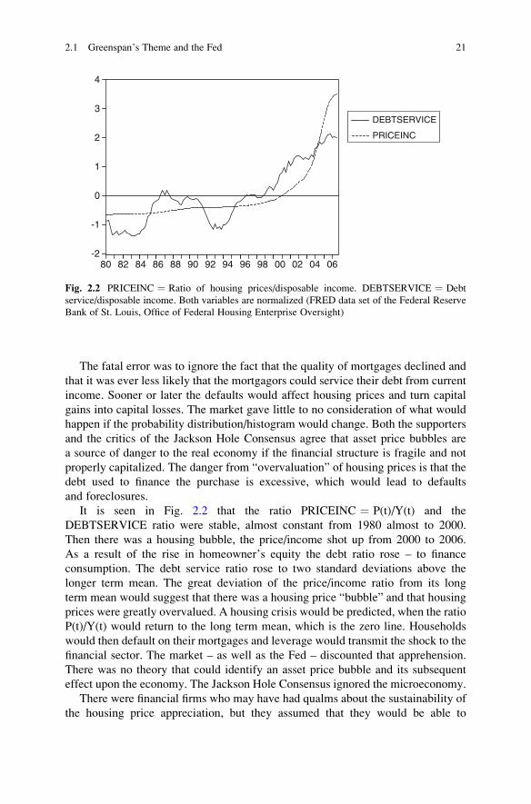
The fatal error was to ignore the fact that the quality of mortgages declined and

that it was ever less likely that the mortgagors could service their debt from current

income. Sooner or later the defaults would affect housing prices and turn capital

gains into capital losses. The market gave little to no consideration of what would

happen if the probability distribution/histogram would change. Both the supporters

and the critics of the Jackson Hole Consensus agree that asset price bubbles are

a source of danger to the real economy if the financial structure is fragile and not

properly capitalized. The danger from “overvaluation” of housing prices is that the

debt used to finance the purchase is excessive, which would lead to defaults

and foreclosures.

It is seen in Fig. 2.2 that the ratio PRICEINC ¼ P(t)/Y(t) and the

DEBTSERVICE ratio were stable, almost constant from 1980 almost to 2000.

Then there was a housing bubble, the price/income shot up from 2000 to 2006.

As a result of the rise in homeowner’s equity the debt ratio rose – to finance

consumption. The debt service ratio rose to two standard deviations above the

longer term mean. The great deviation of the price/income ratio from its long

term mean would suggest that there was a housing price “bubble” and that housing

prices were greatly overvalued. A housing crisis would be predicted, when the ratio

P(t)/Y(t) would return to the long term mean, which is the zero line. Households

would then default on their mortgages and leverage would transmit the shock to the

financial sector. The market – as well as the Fed – discounted that apprehension.

There was no theory that could identify an asset price bubble and its subsequent

effect upon the economy. The Jackson Hole Consensus ignored the microeconomy.

There were financial firms who may have had qualms about the sustainability of

the housing price appreciation, but they assumed that they would be able to

-2

-1

0

1

2

3

4

80 82 84 86 88 90 92 94 96 98 00 02 04 06

DEBTSERVICE

PRICEINC

Fig. 2.2 PRICEINC ¼ Ratio of housing prices/disposable income. DEBTSERVICE ¼ Debt

service/disposable income. Both variables are normalized (FRED data set of the Federal Reserve

Bank of St. Louis, Office of Federal Housing Enterprise Oversight)


anticipate the onset of a crisis in time to retrench. Charles Prince’s remark is

emblematic: “When the music stops, in terms of liquidity, things will be compli-

cated. But as long as the music is playing, you’ve got to get up and dance”.

They certainly were mistaken, because they ignored systemic risk that the negative

shock could be pervasive, and liquidity and capital would disappear in the wake of a

mass exodus from the markets for derivatives.

There were a few hedge firms such as Scion Capital (SC) that anticipated the

crash and took appropriate actions. Michael Burry (2010) of SC realized in 2005

that the bubble would burst and acted upon that view. He purchased credit default

swaps (CDS) on billions of dollars worth both of subprime mortgage backed

securities and bonds of many financial corporations that would be devastated

when the real estate bubble burst. Then as the value of the bonds fell, the value

of CDS would rise. The investors in his hedge fund still “wanted to dance” and

profit from the rising house prices. Despite pressure from the investors, Burry

liquidated the CDS at a substantial profit. But since he was operating in face of

strong opposition from both his investors and from the Wall Street community, he

shut down SC in 2008. Greenspan responded negatively to Burry’s predictions and

suggested that Burry was just lucky. Lowenstein (2010, Chap. 7) describes the

divergent opinions in the market where the pessimists were in the minority.

2.1.5 The Controversy Over Regulation and Deregulation

In the years prior to the crisis there was a controversy concerning the regulation of

Over the Counter (OTC) markets for derivatives in particular. The warnings and

issues raised were disregarded and strongly opposed by the Fed and Treasury.

The warnings were public information. After the crisis, the disregarded policies

were embodied in the Dodd-Frank bill. The errors of Greenspan, Rubin were of

those of commission not omission.

I draw upon the FCIC report to explain the controversy. Derivative markets are

organized as exchanges and as OTC markets. Exchanges are regulated by Federal

law and play an important role in the price discovery process. They reveal as public

information market anticipations of commodity prices and of interest rates under-

lying futures and derivatives. See Stein (1986) for the economics of futures

markets. OTC derivatives are traded by large financial institutions – traditionally

bank holding companies, investment banks – which act as derivatives dealers,

buying and selling contracts with the customers. Unlike futures and options

exchanges, the OTC market is neither centralized nor regulated. The price discov-

ery process is limited. The OTC market is opaque.

In May 1998 Commodities Futures Trading Commission (CFTC) chairman

Brooksly Born said that the agency would reexamine the way it regulated the

OTC derivatives market. The US General Accounting Office (GAO) issued a report

on financial derivatives that found systemic risks and dangers in the concentration

of OTC derivative activity among 15 major dealers. The GAO concluded that “the


sudden failure or withdrawal of any one of these dealers could cause liquidity

problems in the markets and could also pose risks to the others, including federally

insured banks and the system as a whole”.

The Treasury, Fed and SEC – Greenspan, Rubin, Levitt and Summers opposed

regulation. Greenspan said “. . .regulation of derivatives transactions that are pri-

vately negotiated by professionals is unnecessary”. He continued to advocate

deregulation of the OTC market and the exchange traded market. Greenspan

believed that: “By far the most significant event in finance during the past decade

has been the extraordinary development and expansion of financial derivatives.”

In 1999 the President’s Working Group on Financial Markets, a committee of

the heads of the Treasury, the Federal Reserve, SEC and CFTC charged with

tracking the financial system, chaired by Summers, essentially adopted Greenspan’s

view. The group issued a report urging Congress to deregulate OTC derivatives

broadly and reduce CFTC regulation of exchange traded derivatives as well.

In December 2000, in response, Congress passed and President Clinton signed

the Commodities Futures Modernization Act (CFMA) of 2000. This act in essence

deregulated the OTC derivatives market and eliminated oversight, regulation by

both the CFTC and SEC.

The Act let derivatives traders, including large banks and investment banks,

increase their leverage. A key OTC derivative in the financial crisis was the Credit

Default Swap (CDS). This is a type of “insurance” against capital losses on assets.

I discuss the role of CDS in Chap. 6. After the CFMA was passed, the N.Y. State

Insurance Department determined that “naked” CDS did not count as insurance and

therefore was not subject to regulation.

When an insurance company sells a policy, insurance regulators require that

the company set aside reserves in case of loss. In the housing boom, CDS were

sold by firms that failed to put up any reserves, or collateral to hedge their

exposure. In the run up to the crisis of 2007–2008, AIG – the largest US insurance

company – accumulated one-half a trillion dollar position in credit risk through

the OTC market without being required to post even one dollar of initial capital or

making any other provision for loss. AIG was not alone.

The value of the underlying assets for CDS outstanding worldwide grew from

$6.4 trillion at the end of 2004 to $58.2 trillion at the end of 2007. A significant

portion was apparently speculation in “naked” CDS. In addition, much of the risk of

CDS and other derivatives were concentrated in a few of the very large banks and

others such as AIG Financial Products.

Among those who warned of systemic problems was Sheila Blair, Chairman

of the FDIC. She focused upon the ultimate source of the problem – the

mortgages – and the banking sector. She said: “Subprime lending was started

and the lion’s share occurred in the nonbank sector. But it clearly created

pressures on the banks. . .I think nipping this thing in the bud in 2000 and 2001

with some strong consumer rules applying across the board that just simply said

you’ve got to document a customer’s income to make sure they can repay the

loan. . .just simple rules like that”. At the Fed, it was well known that Greenspan

was not interested in increased regulation.


The danger of systemic risk, resulting from the financial structure of derivatives,

was public information that was disregarded by the markets, the Fed and Treasury

and the regulators. I discuss these issues in Chap. 3 on the Quants.

Ex-post the Dodd-Frank (D-F) bill tried to rectify the earlier disregard of the

warnings. The main provisions of the D-F bill are as follows. First, it aims to

create transparency and accountability for derivatives. Second, it aims to close

“Regulatory Gaps”. It provides the SEC and CFTC with authority to regulate

over-the-counter derivatives so that excessive risk-taking can no longer escape

regulatory oversight. Third, it requires central clearing and exchange trading for

derivatives that can be cleared and provides a role for both regulators and

clearing houses to determine which contracts should be cleared. Fourth, it

concerns market transparency. It requires data collection and publication through

clearing houses or swap repositories to improve market transparency and provide

regulators important tools for monitoring and responding to risks. Fifth, it

concerns financial safeguards. It adds safeguards to system by ensuring that

dealers and major swap participants have adequate financial resources to meet

responsibilities, and provides regulators the authority to impose capital and

margin requirements on swap dealers. It aims to ends the possibility that

taxpayers will be asked to write a check to bail out financial firms that threaten

the economy, by creating a safe way to liquidate failed financial firms and

imposing new capital and leverage requirements that make it undesirable to get

too big. It updates the Fed’s authority to allow system-wide support but no longer

props up individual firms. It establishes rigorous standards and supervision to

protect the economy and American consumers, investors and businesses.

Finally, it seeks an advance warning system. It creates the Financial Stability

Oversight Council to identify and address systemic risks posed by large, complex

companies, products, and activities before they threaten the stability

of the economy. The Council is chaired by the Treasury Secretary and includes

the Federal Reserve Board, SEC, CFTC, OCC, FDIC, the new Consumer Finan-

cial Protection Bureau, and an independent appointee with insurance expertise.

Nonvoting members include state banking, insurance, and securities regulators.

The D-F bill attempts to reverse the policies of Geenspan, the Fed and Rubin.

2.1.6 The Failures of International MonetaryFund Surveillance

The Independent Evaluation Office (IEO 2011) of the IMF found that the IMF

provided few clear warnings about the risks and vulnerabilities associated

with the crisis before its outbreak. I basically quote directly from this important

report. The IMF economists tended to hold in the highest regard macro models

of the academic economics profession. These models proved inadequate for

analyzing financial linkages. Specifically, they introduced money and asset


markets in the most rudimentary way, completely unrelated to economic reality.

The failure of the IMF surveillance, discussed in this section, is in fact prima facie

evidence of the failure of the dominant macroeconomic models.

The Fund missed key elements that underlay the developing crisis. In the US

it did not discuss, until the crisis already erupted, the deteriorating lending

standards for mortgage financing nor did the Fund adequately assess the risks

and impact of a major housing price correction on highly leveraged financial

institutions. As late as April 2006, shortly before US housing prices peaked, the

Fund Surveillance reports explained away the rising share of non-traditional

mortgages in the US by writing “Default rates on residential loans have been

low historically. Together with the securitization of the mortgage market, this

suggests that the impact of a slowing housing market on the financial sector is

likely to be limited.”

The Fund’s reading of the financial sector was remote from reality. In 2007

the Fund concluded that the financial sector was sound: “Core commercial and

investment banks are in a sound financial position, and systemic risks appear to be

low. Profitability and capital adequacy of the banking system are high by interna-

tional standards. . ..market measures of default risk have remained benign”.

A remarkable failure of the Fund concerns Iceland before its major financial

crisis. In spite of a banking sector that had grown from about 100% of GDP

in 2003 to almost 1,000% in 2007, this was not noted as a vulnerability that

needed to be addressed urgently. The staff reports about Iceland were sanguine.

The report stated “Iceland’s medium-term prospects remain enviable.” In fact,

“the banking sector appears well-placed to withstand significant credit and

market shocks”.

The IEO explains why the IMF failed to give clear warnings. There was

groupthink, a tendency among homogeneous cohesive groups to consider issues

only within a certain paradigm and not challenge its basic premises. They were

in awe of the dominant macroeconomic models mentioned above. The basic

premises were that market discipline and self-regulation would be sufficient

to stave off serious problems in financial markets. Crises were unlikely to happen

in advanced economies where sophisticated financial markets could thrive with

minimal regulation. The Fund accepted the same inappropriate macroeconomic

model that dominates the academic profession.

Added to groupthink was the confirmation bias which is the tendency of people

to only notice information consistent with their own expectations and ignore

information that is inconsistent with them.

2.2 Conclusions

The crucial ultimate variable is the household debt, the mortgage debt. The rest of

the financial system rested upon the ability of the mortgagors to service their debts.

Systemic risk relates the effects of the failure of the mortgagors to service their

2.2 Conclusions 25

debts upon the financial structure based upon the income from mortgages.

The leverage of the financial system transmitted the housing market shock into a

collapse of the financial system.

A bubble is in effect a large positive unsustainable excess debt. Detection of a

bubble corresponds to the detection of an “excess debt”. The latter is equal to the

difference between the actual and the optimal debt. The fundamentals are reflected

in the optimal debt. The aim of this book is to derive an optimal leverage, debt or

capital requirement. The technique of analysis is Stochastic Optimal Control

(SOC). This analysis balances the expected growth against risk. Thus an excess

debt corresponds to a situation where asset prices deviate from the derived

fundamentals. There is no use of an arbitrary jump process where a crash occurs.

Instead the SOC analysis implies that the probability of a crisis is directly related to

the measured excess debt.

The housing price bubble, its subsequent collapse and the financial crisis were

not predicted either by the market, the Fed, the IMF or the regulators in the years

leading to the current crisis. Warnings, based upon publicly available information,

were not only disregarded but the Fed and Treasury rejected the warnings. They

successfully advocated deregulation of OTC markets. As a result, transparency of

prices was reduced, risk was concentrated in a few major financial institutions and

high leverage was induced. These were basic ingredients for the subsequent crisis.

The Fed, the IMF and Treasury lacked adequate tools which might have

indicated that asset values were vastly out of line with fundamentals. The Fed

and the Fund were not searching for such tools because they did not believe that

they could or should look for misaligned asset values or excess debt, despite

warnings from Shiller, some people in the financial industry, the GAO, state bank

regulators and FDIC. The Fed was blind-sided by the Jackson Hole Consensus

which gave them great comfort in adopting a hands off position. So it was not just a

lack of appropriate tools which undid the Fed; it was a complete lack of apprecia-

tion of what its role should be to head off an economic catastrophe. Peter Clark

wrote that there are two separate but related questions: Are identification and

containment of a financial bubble legitimate activities of the Fed, and if they are,

what are the best tools to carry out this analysis? As the Fed answered “No” to the

first question, it saw no need to address the second question.

References

Bernanke, Ben. 2005. Testimony to congress joint economic committee, October.Burry, Michael J. 2010. I saw the crisis coming. Why didn’t the fed?. New York Times April 4,

2010, Op/Ed page.

Clark, Peter. 2009. Comment on tale of two debt crises. Economics, The Open-AssessmentE-Journal, http://www.economics-ejournal.org/economics/discussionpapers/2009–44.

Congressional Oversight Panel. 2009. Special report on regulatory reform, Washington DC,

January.


Demyanyk, Yulia, and Otto Van Hemert. 2007. Understanding the subprime mortgage crisis.

SSRN: <http://ssrn.com/abstract¼1020396>Financial Crisis Inquiry Report, FCIC Final Report of National Commission. 2011.


and debt. Journal of Banking and Finance 28: 979–996.FRED, Federal Reserve Bank St. Louis, Economic Data Set.

Gerardi, K., A. Lehnert, S. Sheelund, and P. Willen. 2008. Making sense of the subprime crisis.

Brookings Papers, Fall.Greenspan, Alan. 2004a. Understanding household debt obligations. Washington, DC: Remarks

at Credit Union National Association.

Greenspan, Alan. 2004b. The mortgage market and consumer debt. Washington, DC: Remarks at

America’s Community Bankers Annual Convention.

Greenspan, Alan. 2008. Testimony on sources of financial crisis. House committee on governmentoversight and reform.

Greenspan, Alan. 2010. The crisis. Brookings Papers.International Monetary Fund. 2007. World Economic and Financial Survey, Global Financial

Stability Report.

Issing, Otmar. 2009. Asset Prices and Monetary Policy. Cato Journal, 29.

Koopmans, T., and A. Bausch. 1959. Selected topics in economics involving mathematical

reasoning. SIAM Review 1(2): 79–148.

Lowenstein, Roger. 2010. The end of Wall Street. New York: Penguin Press.

OFHEO. 2010. House price indexes, Washington, DC.

Shiller, Robert. 2007. Understanding recent trends in house prices and home ownership. Cowles

foundation discussion paper #1630.

Stein, Jerome L. 1986. Economics of futures markets. New York: Blackwell.

References 27

Chapter 3

Failure of the Quants

Abstract The Quants made several interrelated errors. They based the expected

house price upon the current price and drift, and assumed that the distribution of

capital gains is unchanging. The Quants ignored publicly available information in

forming expectations. The ultimate determinant of the values of CDOs was the

ability of the mortgagors to service their debts. It was public information that

the mortgages were of most dubious value, no due diligence was performed in

the ratings and the debt/income of the mortgagors was rising. Hence it was

improbable that the distribution of house prices would remain constant. Systemic

risk was ignored by the Quants who just focused upon current prices. Ratings of the

tranches were not based upon the quality of the underlying mortgages. They were

all in the same bundle. The rating depended upon who got paid first in the stack of

loans. The key question was how to rate and price the tranches. The issue concerned

the correlation of the tranches. If a pool of loans started experiencing difficulties,

and a certain percent of them defaulted, what would be the impact upon each

tranche? The “apples in the basket model” made one prediction. Another very

different one is “the slice of bread in the loaf” model.

This chapter considers the role of the “Quants” in the crisis. The financial system is

an intermediary between savers and investors. Mathematics is essential to price

securities traded by savers, intermediaries and investors, and to adjust risk to the

preferences of savers and investors. Assets are priced according to the principle that

the price should be equal to the expectation of the present value of the future

income. The future income stream and time profile of future interest rates are

crucial variables, but they are stochastic and unknown when the pricing decision

is made. Similarly the pricing of longer-term bonds depends upon the expectations

of future short term interest rates. This pricing is based upon the term structure

hypothesis that the long rate is a geometric average of future short rates.


29

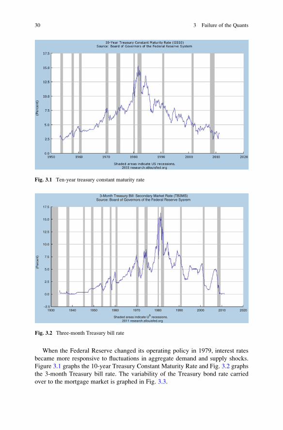
When the Federal Reserve changed its operating policy in 1979, interest rates

became more responsive to fluctuations in aggregate demand and supply shocks.

Figure 3.1 graphs the 10-year Treasury Constant Maturity Rate and Fig. 3.2 graphs

the 3-month Treasury bill rate. The variability of the Treasury bond rate carried

over to the mortgage market is graphed in Fig. 3.3.

Fig. 3.1 Ten-year treasury constant maturity rate

3-Month Treasury Bill: Secondary Market Rate (TB3MS)Source: Board of Governors of the Federal Reserve Sysrem

17.5

15.0

12.5

10.0

7.5

5.0

2.5

0.0

−2.51930 1940 1950 1960 1970 1980 1990 2000 2010 2020

Shaded areas indicate Us recessions.

2011 research.stlouisfed.org

(Per

cent

)

Fig. 3.2 Three-month Treasury bill rate

30 3 Failure of the Quants

As a result of the considerably increased volatility of both short and long term

interest rates there was an increased the demand for risk management. One took a

great speculative risk if a bond position was not hedged.

In the volatile economic climate of the 1970s, trading in financial futures was

introduced. Between 1970 and 1984 futures trading volume increased tenfold and

by the end of 1984 financial futures accounted for 50% of total futures trading. The

Federal Reserve Board (FRB), Securities Exchange Commission (SEC) and

Commodities Futures Trading Commission (CFTC) were directed by an act of

Congress in 1982 to carry out a joint study of the economic purposes of futures and

options markets, to consider their effects upon capital formation, and to evaluate the

adequacy of regulation. I was commissioned to write on the first topic which later

resulted in my book The Economics of Futures Markets (1986). My work seemed to

satisfy the FRB, SEC and CFTC that these markets served useful economic

functions and were not “gambling casinos”.

The interest rate volatility (Figs. 3.1, 3.2, 3.3) above generated a demand by

Wall Street for Quants. The Quants are a group of physicists, mathematicians and

computer science experts who practice “financial engineering”. They develop and

apply models to devise derivatives that would permit the risks to be hedged to an

optimal extent, making the new securities attractive to both savers and investors.

The channeling saving to investment is important for the growth process.

30-Year Conventional Mortgage Rate (MORTG)Source: Board of Governors of the Federal Reserve System

20.0

17.5

15.0

12.5

10.0

7.5

5.0

2.51970 1975 1980 1985

Shaded areas indicate US recessions.2011 research.stlouisfed.org

(per

cent

)

1990 1995 2000 2005 2010 2015

Fig. 3.3 Thirty-year conventional mortgage rate

3 Failure of the Quants 31

3.1 Theme of This Chapter

According to the Efficient Market Hypothesis (EMH), it is impossible to know

when a bubble is occurring, since current prices reflect all publicly available

information. Only in retrospect, when the bubble bursts is it clear that the prices

were inflated. I show that the EMH did not describe accurately what happened.

Quants missed systemic risk because they ignored publicly available information

concerning the mortgage market. That market was very important in the highly

leveraged and interrelated financial markets. The collapse of the mortgage market

bubble led to the financial collapse.

Section 3.2 is a discussion of leveraging, and leads into a vivid example of the

strategy of the Atlas Fund run by Quants, which was given AAA ratings. At first, this

hedge fund was extremely profitable and then it collapsed. This example illustrates

why the Quants failed. Section 3.3 describes the structure of the derivatives market,

the securitization, interrelationships, the rating agencies and pricing of derivatives.

Section 3.4 describes the crucial underlying models used by the Quants based

upon the No Arbitrage Principle NAP – the CAPM, Black-Scholes-Merton (BSM)

and EMH – in devising their instruments and strategy. Section 3.5, discusses the

models, based upon the No Arbitrage Principle NAP, in detail. Section 3.6 concerns

methods to determine when the drift of the capital gains has changed. The conclu-

sion is Sect. 3.7. It summarizes the errors made by the Quants in the pricing of

the tranches and the Credit Default Swaps. The next few chapters explain why

Stochastic Optimal Control (SOC) uses information much better and can provide

Early Warning Signals (EWS) of a crash.

3.2 Leveraging

It is now widely believed that “excessive” leveraging, and an “excessive” debt

ratio, at key financial institutions helped convert the initial subprime turmoil in

2007 into a full blown financial crisis of 2008. Leverage is the ratio of assets /net

worth A(t)/X(t), or equivalently the ratio of debt L(t) to net worth X(t) denoted

f(t) ¼ L(t)/X(t). Although leverage is a valuable financial tool, “excessive” leverage

poses a significant risk to the financial system. For an institution that is highly

leveraged, changes in asset values greatly magnify changes in net worth. To main-

tain the same debt ratio when asset values fall either the institution must raise more

capital or it must liquidate assets.

The relations are seen through Equations (i)–(iv). In (i) net worth X(t) is equal to

the value of assets A(t) less debt L(t). Equation (ii) is just a way of expressing the

debt ratio. Equation (iii) relates the debt ratio f(t) ¼ L(t)/X(t) to the leverage ratio

A(t)/X(t) of assets/net worth. Equation (iv) states that the percent change in net

worth dX(t)/X(t) is equal to the leverage (1 + f(t)) times dA(t)/A(t) the percent

change in the value of assets.


(i) X tð Þ ¼ A tð Þ � L tð Þ:(ii) L tð Þ=X tð Þ ¼ f tð Þ ¼ 1=½ðA tð Þ=L tð Þ � 1�:(iii) A tð Þ=X tð Þ ¼ 1þ f tð Þ:(iv) dX tð Þ=X tð Þ ¼ 1þ f tð Þð Þ dA tð Þ=A tð Þ:

The Congressional Oversight Panel (2009) (COP) reported that, on the basis of

estimates just prior to the crisis, investment banks, securities firms, hedge funds,

depository institutions, and the government sponsored mortgage enterprises –

primarily Fanny Mae and Freddie Mac – held assets worth $23 trillion on a base

of $1.9 trillion in net worth, yielding an overall average leverage of A/X ¼ 12.

The leverage ratio varied widely as seen in (Table 3.1).

Consider the average leverage, where A(t) ¼ $23 trillion, X(t) ¼ $1.9 trillion,

L(t) ¼ $21.1 trillion, making the debt ratio f ¼ 11.1. From Equation (iv), a 3%

decline in asset values would reduce net worth by dX(t)/X(t) ¼ (1 + 11.1)

(0.03) ¼ 36%. The loss of net worth is equal to (0.36) ($1.9 trillion) ¼ $0.69

trillion. To maintain the same ratio f ¼ 11, the institutions must either raise capital

to offset the decline in asset values dX ¼ dA < 0, or must sell off assets to reduce

debt by the same proportion dL(t)/L(t) ¼ dX(t)/X(t), derived from Equation (ii).

A 3% decline in asset value would require the sale of (0.03) (21.1 trillion) ¼ $630

billion in assets to repay the debt.

Both actions have adverse consequences for the economy. Firms in the financial

sector, the financial intermediaries, are interrelated as debtors-creditors. Banks lend

short term to hedge funds who invest in longer term assets and who may also buy

credit default swaps. Firms that lost $690 billion in net worth would have difficulty

in raising capital to restore their net worth, without drastic declines in share prices.

Similarly, the attempt by one group to sell $630 billion in assets to repay loans will

have serious repercussions in the financial markets. The prices of these assets will

fall, and the leverage story repeats for other groups. Institutions who hold these

assets will find that the value of their portfolios have declined, reducing their net

worth. In some cases, there are triggers. When the net worth of a Fund falls below

a certain amount (“breaks the buck”) the fund must dissolve and sell its assets,

which may include AAA assets. In turn the sale of AAA assets affects other

institutions. Conservative investors may have thought they were holding very

safe assets, but to their dismay they suffer capital losses as AAA assets are

liquidated at “fire sale” prices. In a highly interrelated system, “high leverage”

can be very dangerous. What seems like a small shock in one market can affect

via leverage the whole financial sector. The Fed and the IMF seemed oblivious to

this systemic risk phenomenon because of the history of two previous bubbles.

Table 3.1 Leverage

of institutionsBroker-dealers and hedge funds 27

Government sponsored enterprises 17

Commercial banks 9.8

Savings banks 6.9

Average, weighted 12

3.2 Leveraging 33

In the S&L and agricultural crises of the 1980s, discussed in Chap. 7, there was not

a strong linkage between the specific sector and a highly leveraged interrelated

financial sector based upon CDO and CDS. Therefore the collapse of these earlier

bubbles only had localized effects.

3.2.1 The Incredible Leverage of Atlas Capital Funding

The story of the Atlas Capital Fund is an excellent example of leveraging discussed

above. My discussion is based upon a paper given by Jichuan Yang, one of

the principals of Atlas, given at an Applied Mathematics Colloquium at Brown

University in September 2009 and the paper by RenCheng (former Chief Investment

Officer at Fidelity) at the same Colloquium. A group of talented financial engineers:

mathematicians, physicists specializing in mathematical finance, decided to

establish a Fund in 2003 with $12 billion of assets, and $10 million of capital, –

a leverage of 1,200. This Fundwas called the Atlas Capital Fund, due to its huge size.

The fund portfolio would contain thousands of individual bonds, loans and other

financial securities that had longer term maturities, such as 8 years. The liabilities

were commercial paper and mid-term notes with maturities ranging from 30 days to

5 years. Atlas would borrow short term and lend longer term to the Hedge Funds.

The Fund was not set up to hedge risk but to seek maximum return. The Fund did not

fear taking risk. Atlas wouldmake its profits from the difference between the lending

rate charged to the hedge funds and the cost of short term borrowing. The latter could

be reduced to aminimum if Atlas received aAAA rating. This was a remarkable goal

because most global banks are rated no higher than AA.

Since the portfolio had a much longer maturity than the loans, a major risk to

Atlas would be the variable short term borrowing rate. Figure 3.2 graphs the

volatility of the short term interest rate. When the 30-day loan matured, Atlas

would roll over the 30-day loan at the current rate. If there were difficulties in

rolling over, Atlas would have to find banks, called “liquidity providers”, to give

Atlas “emergency” loans to pay off the 30-day debt.

The “financial engineers” built a model to evaluate the risk, which they used to

convince the rating agencies to give them an AAA rating, which lowers the cost of

borrowing. The model simulated the movement of the $12 billion of individual

assets as well as their correlated behavior. The mismatch of the timing of cash flows

of assets and liabilities, the price movements, the rating changes, the defaults and

recovery had to be “accurately” modeled, calculated and simulated. For each

potential future price movement, the model calculated the gain, loss and return.

After tens of thousands of such simulations, the financial engineers arrived at an

estimate of the expected loss and expected return by certain types of averaging the

individual outcomes. These simulations convinced the rating agencies to give Atlas

an AAA rating and hence a low cost of borrowing.


At first, Atlas was extremely profitable. Stockholders received 100% of their

money back in the first year of operations due to the leverage of 1,200, equal to $12billion of assets/$10 million of capital. The Fed was most accommodating with its

low interest policy. Moreover, Chairman Alan Greenspan was the champion of

financial innovation and was fighting off regulatory reform on all fronts, as

discussed in Chap. 2. About 3 years after Atlas started operations, the US financial

industry went into one of its worst crises. The cascading effects of leverage

discussed above then occurred. Atlas was blamed as being one of the main culprits

causing the crisis. Jichuan Yang, a principal of Atlas, wrote in 2009: “Today, if

someone tells me that all these things can be simulated by an elegant mathematical

model with any realistic accuracy, I would be tempted to say that he’s probably an

overconfident idiot”.

3.3 Structure of Derivatives Market, Rating Agencies

and Pricing of Derivatives

This part draws upon the comprehensive FCIC report, and the books by Derman

and by Patterson. The financial market consisted of several stages. At one end were

the mortgagors, the households who borrowed against negligible collateral or

ability to service the loans from income, the NINJAs (no income no jobs, no assets).

Their loans were packaged or securitized into bundles by financial intermediaries

who could not perform due diligence because they had no idea of the quality of the

loans. In turn, these packages were sold to institutional investors, who relied upon

the rating agencies to evaluate risk. This method was used by FNMA and then

followed by the private sector.

Vast quantities of similar but not identical securities were pooled into bundles

and sold to large investors, mutual funds, pension funds, insurance companies and

hedge funds who were seeking high return and low risk investments. There was no

clear way to evaluate the risk of a package, because it consisted of many mortgages

of dubious quality. However, it was believed that by pooling the securities the risk

would be diversified. There would be losses on the poor quality ones but the returns

on the high quality mortgages would be uncorrelated with the poorly performing

group. That is, the bundle would be like apples in a basket. There will be some

rotten ones, but there would also be good ones. The process of asset acquisition,

pooling and standardization would be attractive to investors. There was a belief in

geographic diversification and that real estate markets are local ones/independent.

This belief reflected the fact that nationwide real estate price declines had not been

experienced since the Great Depression. The banks, the original owners of the

mortgages, sold them to the investment houses that securitized the packages, and

could make more loans. The supply of mortgages would then be increased, just as

the demand was increased by the risk diversification packages. Greenspan believed

3.3 Structure of Derivatives Market, Rating Agencies and Pricing of Derivatives 35

that: “By far the most significant event in finance during the past decade has been

the extraordinary development and expansion of financial derivatives.”

The Quants devised a method to sell the derivatives of dubious value as AAA

securities. A prioritization method was used. Tranches of the pool were sold, like

bonds, preferred stock and common stock in the same bundle. Losses or defaultswould first affect the lowest tranche (Equity) then when that tranche’s assets were

exhausted, the losses would affect the medium (Mezzanine) tranche. The top, senior

tranche (AAA) would only lose if the losses exceeded the assets in all the tranches.

Ratings were not based upon the quality of the underlying mortgages all of

which were in the same bundle. The rating depended upon who took losses first in

the stack of loans. The rating agencies were essential to the smooth functioning of

the mortgage backed securities market. Banks needed their ratings to determine the

amount of capital to hold, repo markets needed the ratings to determine loan terms,

and some investors could only buy securities with a AAA rating. Credit ratings also

determined whether investors could buy certain investments. The SEC restricts

money market funds to purchasing securities that have received credit ratings in one

of the two highest short-term rating categories. The Secondary Mortgage Market

Enhancement Act of 1984 permitted federal and state chartered financial

institutions to invest in mortgage related securities if the securities had high credit

ratings from at least one rating agency. Many investors, such as pension funds and

university endowments relied on credit rating agencies because they had neither

access to the same data as the rating agencies nor analytical ability to assess the

securities that they were purchasing.

The logic of trenching was the apples in a basket model. The loaf of breadmodel, discussed in my criticism below, was not considered. Say that there were

two tranches A(AAA, top) and B (Equity, bottom). Let 1 > p > 0 be the proba-

bility of default of the entire package. The losses first affect tranche B. Tranche A

can only suffer losses if tranche B is wiped out.

The probability Pr(B) of default of tranche B is 1 > p > 0. The probability that

that both tranches suffer losses is Pr(AB). In the Apples in a Basket case the defaultsin the two tranches are independent samples of apples from a population (basket)

where the probability of default is p. A first apple (Equity or Mezzanine tranche) is

taken from the basket and it turns out to be rotten. This will occur with probability p.

A second apple (Senior tranche) is taken out of the basket. In the “basket of apples”

case, the Pr(A|B) ¼ Pr(B) ¼ p. In this case of independence, the probability that

both apples are rotten corresponds to the case where the senior tranche would

be exhausted Pr(AB) ¼ Pr(A)Pr(B) ¼ p2 < p. Risk of the senior tranche is less

than that of the entire package. The senior tranche appeared to be a silk purse made

from a sow’s ear.

Since the mid-1990s Moody’s has rated tranches of mortgage backed securities

using several models. Although Moody’s did not sample or review individual loans,

the company used loan/value ratios, borrower credit scores and loan terms.

The model simulated the performance in 1,250 scenarios including variations in

interest rates and state unemployment rates as well as in home price changes.

Thereby ratings were given to the tranches.


On average across the scenarios, home prices trended upwards at approximately

4% per annum. The model put little weight on the possibility that prices would fall

sharply nationwide. Even as house prices rose to unprecedented levels, Moody’s

never adjusted the scenarios to put greater weight on the possibility of a decline.

This choice did not consider that there was a national housing bubble and did not

sufficiently account for the deterioration of the quality of loans securitized.

In October 2007, Moody’s downgraded all of the mortgage backed securities that

it had rated AAA in 2006, and downgraded 73% to junk. There was indeed a house

price bubble. The obvious question is why was the rating system a failure?

3.3.1 Pricing CDOs

Ratings of the tranches were not based upon the quality of the underlying

mortgages. They were all in the same bundle. The rating depended upon who got

paid first in the stack of loans. The key question was how to rate and price the

tranches. The issue concerned the correlation of the tranches. If a pool of loans

started experiencing difficulties, and a certain percent of them defaulted, what

would be the impact upon each tranche? The “apples in the basket model” made

one prediction. Another very different one is “the slice of bread in the loaf” model.

The slices of bread model assumes systemic risk, in which the value/returns of

assets are very highly or perfectly correlated. The probability of having moldy

slices in the package is 1 > p > 0. If the first slice (B) taken from the loaf is moldy,

what is the probability that the second one (A) is also moldy? The conditionalprobability that assets in tranche A (second adjacent slice is moldy) default, given

that B defaults (first slice is moldy) is close to unity, Pr(A|B) ¼1. In this case,

the probability that the owners of tranche A lose is Pr(AB) ¼ Pr(A|B) Pr(B) ¼1.Pr(B) ¼ p. The senior tranche is as risky as is the average of assets in the

portfolio. Tranching/securitization can allow risk reduction only if there is no

systemic risk. With systemic risk, where Pr(A|B) ¼ 1 or close to it, the whole

structure can collapse. If B defaults one is confident that A will default.

Since there were many assets in the CDO and no due diligence was performed, it

was extremely difficult or impossible to evaluate the correlations or conditional

probabilities of defaults among tranches. Because there was no organized exchange

for the CDOs, their market prices were not transparent. No one knew what they were

worth if sold on themarket. This was the challenge for theQuants and rating agencies.

The “solution” was Li’s copula/CDS model. One would know if they viewed

“the apples in the basket” or “slices of bread” case as more relevant. In the “slices of

bread” case, there was no point in correlating tranches. Only the probability p that

the package will default is relevant.

The CDS rate was linked closely with house prices. Because the CDO boom was

occurring at the same time as the housing prices were inflating, the CDS showed

very little risk. In fact, there was a positive feedback between the CDS rate and

housing prices. The rise in house prices lowered the CDS rate on the tranches

3.3 Structure of Derivatives Market, Rating Agencies and Pricing of Derivatives 37

and the packages of tranches increased in value. This increased the demand for

mortgages by the securitizers, which in turn induced a greater supply of mortgages

of any quality. Thereby housing prices rose further.

3.4 Major Premise of Economics/Finance:

No Arbitrage Principle (NAP)

The Quants relied upon three models: the CAPM, the Black-Scholes-Merton

Options pricing model (BSM) and the Efficient Market Hypothesis (EMH) to

price securities and manage risk. The first two models are logical deductions

from their premises. The BSM was a brilliant synthesis of mathematics and

economics. Both the CAPM and BSM were based upon the major premise in

economics and finance: the No Arbitrage Principle (NAP).The NAP is the foundation of microeconomic household and firm optimization.

A main principle in economics is that the gain per dollar spent on a consumer good

should be the same for all goods consumed. Similarly in the theory of the firm, the

gain per dollar spent on an input in the production process should be the same for all

inputs used. The NAP conditions are expressed as follows. Let the consumer have a

utility function over n-goods or services. The price of each good is known and fixed.

The budget constraint is that the sum of expenditures over the n-goods equals the

given budget. The NAP equation is that the marginal utility per dollar should be the

same for each of the n-goods consumed. The marginal rate of substitution in utility

(along the indifference curve or surface) should equal the relative given market

prices (slope of budget line). Utility is thereby maximized subject to the budget

constraint. If the relative marginal utilities are given, the relative prices are deter-

mined, and vice-versa.

In the theory of the firm, a known production function relates inputs to output.

For a given cost, the inputs used should be such that their marginal product per

dollar of input price be equal for each input used. Equivalently, the marginal cost to

produce output (price input/marginal product) should be the same for all inputs

used. If one knows the relative marginal productivities, then relative input prices

are known and vice-versa. This no arbitrage condition NAP minimizes costs for a

given output.

3.4.1 CAPM Model

The no arbitrage condition takes an analogous form in CAPM and Black-

Scholes-Merton models in finance. The NAP principle in the CAPM was derived

by Sharpe (1964) as follows. Let there be a market (m) portfolio of n assets. Each

asset has a return and a risk/variance, and there are n2 variances and covariances.


The market portfolio (designated by “m”) has an expectation m and a variance

sm2, based upon the variance/covariance matrix of the n-assets. There is also a

safe asset with an interest rate of r. One can achieve a combination of expected

returns and risk by combining the market portfolio whose return – risk is (m, sm)

with the safe asset whose return – risk is (r, 0). This linear combination is the

capital market line, where the risk-return trade-off is:

dE=dsm ¼ ðm� rÞ=sm: (3.1)

One can also achieve a risk – return by varying the composition of the market

basket. Let there be a portfolio where fraction a is in asset i and fraction (1�a) is in

the entire market basket of all n ¼ 1,2,. . .i,. . .n-assets. The expected return is E and

the variance is s2 for the portfolio (3.2).

E ¼ aEi þ 1� að Þm variance ¼ s2 (3.2)

As fraction a varies, both the expected return and the risk of the portfolio change.One obtains dE/da and ds/da by varying the composition. Equation 3.3 is the

risk-return trade-off obtained by varying the composition of the portfolio, evaluatedat the optimum portfolio, when a ¼ 0.

f½ðdE=daÞ=ðds=daÞ�ja ¼ 0g (3.3)

The NAP requires that the two risk-return trade-offs be equal. Equation 3.4

equates (3.1)–(3.3).

f½dE=dsm� ¼ ðm� rÞ=smg ¼ fðdE=daÞ=ðds=daÞ�ja ¼ 0g (3.4)

From (3.4) one obtains the CAPM equation (3.5).

½Ei � r� ¼ bi½m� r�; bi ¼ sim=s2m (3.5)

The CAPM provides a good measure of risk. Assets can only earn high average

returns if they have high betas. Average returns are driven by beta because beta

measures the extent that the addition of a small quantity of the asset to a diversified

portfolio adds to the volatility of the portfolio. Beta is estimated by regressing the

observed return of asset i upon the observed return on the total portfolio, each

adjusted for r, the safe rate of return.

3.4.2 BSM Model

The BSM options pricing is based upon the NAP. Fischer Black derived the

equation on the principle: Assets must be priced such that risk per unit of return

is the same for all traded assets. Let there be a stock whose price S(t). The price

3.4 Major Premise of Economics/Finance: No Arbitrage Principle (NAP) 39

change dS(t) is the sum of a drift plus a Brownian Motion (BM) term dw(t), where

E(dw(t)) ¼ 0, E(dw(t))2 ¼ dt. The drift coefficient m and diffusion coefficient s are

constant.

dSðtÞ ¼ mSðtÞdtþ SðtÞsdwðtÞ ¼ drift SðtÞ þ diffusion SðtÞ: (3.6)

There is a derivative whose value V is linked to the price of the stock S(t). There

are several ways to derive and view the BSM equation and I follow the Fleming-

Soner (2006, pp. 360–362) exposition within the NAP. One can buy the derivative

at time t whose value V(t,S) depends upon the stock price at time t, or one can

purchase for the same amount a portfolio of value X(t) ¼ V(t,S), consisting of the

stock and a bond yielding a safe return of r.

The change in the value of the portfolio dX(t), (3.7) is the sum of a drift term and

a diffusion term. Similarly the change in the value of the derivative dV(t) is the sum

of a drift and a diffusion term (3.8).

dXðtÞ ¼ drift XðtÞ þ diffusion XðtÞ (3.7)

dVðt; SðtÞÞ ¼ drift VðtÞ þ diffusion VðtÞ (3.8)

The NAP states that, for the same risk, the change in the value of the portfolio dX

should equal the change dV in the value of the derivative dX(t) ¼ dV(t, S(t)).

Use (3.7) and (3.8) to derive NAP equation (3.9).

drift XðtÞ þ diffusion XðtÞ ¼ drift VðtÞ þ diffusion VðtÞ (3.9)

The NAP requires that both assets having the same risk must have the same

return. Equate drift X(t) to drift V(t) (3.10). This equalizes the return. Equate the

two diffusion terms (3.11). This equalizes the risk. The portfolio composition at

each time must be adjusted to provide an equal risk.

drift X ¼ drift V (3.10)

diffusion X ¼ diffusion V (3.11)

Solve the two equations for the ratio of the stock/portfolio and for the value of

the derivative V. The BSM equation (3.12) for derivative pricing V(t,S(t)) is

derived.

Vt ðt; SÞ þ rSVsðt; sÞ þ ð1=2Þs2S2Vssðt; sÞ ¼ rVðt; SÞ: (3.12)

The main implications of BS are: (a) the drift term m of the stock plays no role in

the pricing. (b) The variance s2 plays a very important role.


3.4.3 The Efficient Market Hypothesis (EMH)

An important hypothesis used in the finance literature is the EMH Efficient Market

Hypothesis. It is based upon the hypothesis that “Properly Anticipated Prices

Fluctuate Randomly”. However, its application to the world of finance with the

derivatives rests upon vague and arbitrary assumptions. This was the fatal flaw.

First I discuss these models and then evaluate their application to the pricing of

derivatives.

The EMH is an empirical application of the hypothesis that “Properly

Anticipated Prices Fluctuate Randomly” (Samuelson 1965). The latter is a set of

mathematical propositions. The EMH has been applied to stock prices and foreign

exchange rates with less than successful verification. I explain later in this chapter

why the attempt to apply it pricing of CDOs, CDS and tranches failed and led to the

bubble and its collapse.

The view underlying the EMH is that in an “informationally efficient” market

price changes must be unforcastable. By “informationally efficient” one means that

the market price fully incorporates the expectations and information of the market

participants (Fama 1970). The mathematical structure of the argument below is

based upon Feller, volume II (1966). It consists of three propositions, any one will

imply the other two.

Let X(t) be the change in price P(t). Equation 3.13 states that the expectation of

the change in price E[X(t)] ¼ 0. This proposition is called an absolutely fair game.

E½XðtÞ� ¼ 0: (3.13)

It reflects the view that, in a competitive market with informed buyers and sellers

trading at market determined prices, if one were sure that a price will rise, it will

already have risen.

Price P(t) is the sum of previous price changes X(s), s < t. It can be expressed as

the previous price P(t�1) plus the current price change X(t) (3.14).

PðtÞ ¼X

XðsÞð Þ ¼ P t� 1ð Þ þ XðtÞ: t � s � 0: (3.14)

The expectation of the price E[P(t)|P(t�1), P(t�2). . .], conditional upon its past

history,

EPðtÞ ¼ EhX

XðsÞÞi¼ P t� 1ð Þ þ EXðtÞ ¼ P t� 1ð Þ

�(3.15)

is (3.15), because (3.13) states that the expectation of a price change E X(t) is zero.

This proposition is the martingale property. The expectation of the next period’s

price is the current price.

The third proposition is called the Impossibility of Systems. It states that no

strategy based upon the past history of prices can be profitable. No system can


produce positive expected profits. Although a system may work at one time, that is

a fluke and what works once is unlikely to work again.

Z(t) is cumulative profits. Let v(t) be a system, a formula, fixed in advance.

It tells one when and how much to buy/sell at any time, based upon the past history

of prices or any other variables. Then Z(t)

ZðtÞ ¼ Zðt� 1Þ þ vðtÞ½PðtÞ � Pðt� 1Þ� ¼ Zðt� 1Þ þ vðtÞXðtÞ: (3.16)

is the sum of the previous cumulative profits Z(t�1) plus the profit from the last

trade, based upon the fixed in advance system v(t).

The expectation of cumulative profits E[Z(t)] conditional upon the past prices is

E½ZðtÞ� ¼ Zðt� 1Þ sinceE½XðtÞ� ¼ 0 (3.17)

It is equal to the previous profits, since the expected price change EX(t) ¼ 0

from (3.13). Any sequence of decision functions converts martingale {P(t)} into

martingale {Z(t)}.

Any one (3.13), (3.15), (3.17), which describes the hypothesis that “Properly

Anticipated Prices Fluctuate Randomly”, implies the other two. This is a mathe-

matical proposition but it does not explain where the basic probability distributions

underlying Expectation E come from. It does not explain what is “Information” nor

does it explain howmarket participants act upon what they think is “information” or

by “risk adjusting” their expectations.

The next section discusses how the market/Quants used these hypotheses in the

world of CDOs, CDS, tranches and options, and how their misuse led to and

aggravated the bubble.

3.4.4 The Quants and the Models

On the basis of the EMH and CAPM, Greenspan, the Fed and the finance profession

believed that markets would be self-regulating through the activities of analysts and

investors. In their view, government intervention weakens the more effective

private regulation.

Securitization/tranching, the various layers of CDOs, and CDS, produced an

environment where the EMH/CAPM lost relevance. These bundles of many mort-

gage based securities seemed to tailor risk for different investors. Securitization/

tranching gave the illusion that one could practically eliminate risk from risky

assets and led to very high leverage, as discussed in the section on the Atlas fund.

In hindsight, it was difficult to understand how tranching the equity tranche – which

consisted of poor prospects – into tranches could produce AAA ratings.


In reference to the LTCM collapse, Derman (p. 190) wrote: “It was a shock to

realize that people whose great experience and knowledge straddled both the

quantitative and trading worlds had, despite their sophistication, brought them-

selves into such a catastrophic state”. The same could certainly be said about the

financial collapse of 2007–2008. How can the latter be explained?

The Quants made several serious errors in modeling. First, there were no

relevant “betas” to measure the risk of the CDOs. Second, the martingale property

of the price is a special case of “The Principle that Properly Anticipated Prices

Fluctuate Randomly”, which does not apply to the house price index. Third, they

ignored the “no free lunch” principle, discussed below, that the expected present

value of an asset must be finite. Fourth, they assumed that there is a stable

distribution function for house prices, from which they could derive the VaR

value at risk. They assumed that the “free lunch” would continue, and invoked a

“Black Swan” to justify their failures Fifth, they ignored the feedback in both

directions between house prices, the price of a CDS, and the debt of households.

Each of these is discussed in turn.

3.4.5 The CAPM

The financial market consisted of several stages. At one end were the mortgagors,

households who borrowed against negligible collateral or ability to service the

loans from income. Their loans were packaged or securitized into bundles by

financial intermediaries who could not perform due diligence since they had no

idea of the quality of the loans. In turn these packages were tranched and sold to

institutional investors, who relied upon the rating agencies to evaluate risk. How

could the risk be evaluated? The CAPM states that it is measured by the beta of the

tranche (3.5) repeated.

½Ej � r� ¼ bj½m� r�; bj ¼ sjm=s2m

To calculate the beta of tranche j one must know, the expected return m on the

larger portfolio containing tranche j, the variance-covariance matrix of all of the

tranches and assets in the larger portfolio, the covariance sjm to between the return

on tranche j and the return on the larger portfolio. These quantities could not be

calculated. There were thousands of mortgages in each tranche, most of them of

dubious value. No due diligence was performed. Their market prices were unknown

so that one could not calculate the Ej the expected return on the tranche. In addition,

what was the market portfolio containing tranche j whose mean was m, whosevariance was sm

2 and covariance was sjm with tranche j?


3.4.6 Credit Default Swaps, EMH and the House Price Index

Since there are many assets in the CDO and no due diligence was performed, it was

extremely difficult or impossible to evaluate the correlations or conditional

probabilities of defaults among tranches. There was no organized exchange for

the CDOs. Their market prices were not transparent. No one knew what they were

worth if sold on the market and internal accounting rules allowed Mark-to-Market

values to be set by internal risk models rather than by verifiable quotes from

transaction. This was a challenge for the Quants and rating agencies.

The “solution” was Li’s copula/CDS model. His model could assign correlations

between the tranches by measuring the Credit Default Swap rate (CDS) linked to

the underlying security. The CDS of the tranches supplied a single variable that

incorporated the market’s assessment of how the tranche will perform. The CDS

rate was linked closely with the prices of the mortgages and CDOs, which in turn

was based upon the house price index. Then one could price the CDOs/tranches

based upon the CDS rate. The important question was how to estimate the expected

house price, in order to price the CDS.

EMH equation (3.15) states that the expected price EP(t + dt) is equal to the

present price P(t), the martingale property. This is only true, however, in special

cases and is not implied by the NAP. For example, the spot price of a harvest

commodity is not a martingale, whereas the futures price is a martingale (Stein

1986; Samuelson 1957).

Inventories rise as the harvest comes in. The balance of short hedging by those

carrying inventories lowers the spot price below the price expected at a later date,

due to a risk premium and storage costs. As inventories decline, short hedging

declines and the spot price rises towards the expected price. Thus P(t) is less than

EP(t + dt) and its expected change E[dP(t)] is not zero.

Similarly, before the harvest there is a balance of long hedging, by those who

want to protect themselves from later purchases at higher prices. The spot price P(t)

rises above the expected price, due to a risk premium and very low inventories.

As the harvest comes in, there is a decline in long hedging, and the spot price

declines. Thereby P(t) is greater than EP(t + dt) and its expected change E[dP(t)] is

not zero. The NAP is not violated. In both cases however, the futures price is tied to

EP(t + dt) and is a martingale.

In the case of the CDS, the variable to consider is the index of house price P(t).

Let the house price follow a random walk with drift, equation

dPðtÞ ¼ mPðtÞdtþ PðtÞsdwðtÞ ¼ driftþ diffusion;E½dw� ¼ 0; E dw2� � ¼ dt:

(3.18)

The drift coefficient, the trend, is m and the diffusion is s dw(t). The CDS rate is

based upon the expected house price index. Solve (3.18) for P(t), using the Ito

equation to derive (3.19). Take the expectation and derive (3.20).


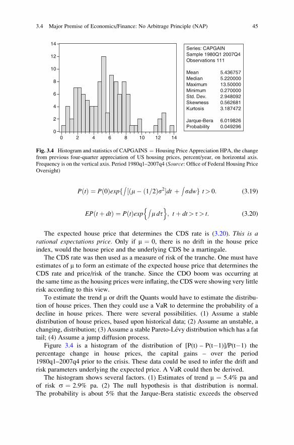
PðtÞ ¼ Pð0ÞexpfZ½ðm� 1=2ð Þs2�dt þ

Zsdwg t> 0: (3.19)

EP tþ dtð Þ ¼ PðtÞexpZm dt

n o; tþ dt> t> t: (3.20)

The expected house price that determines the CDS rate is (3.20). This is arational expectations price. Only if m ¼ 0, there is no drift in the house price

index, would the house price and the underlying CDS be a martingale.

The CDS rate was then used as a measure of risk of the tranche. One must have

estimates of m to form an estimate of the expected house price that determines the

CDS rate and price/risk of the tranche. Since the CDO boom was occurring at

the same time as the housing prices were inflating, the CDS were showing very little

risk according to this view.

To estimate the trend m or drift the Quants would have to estimate the distribu-

tion of house prices. Then they could use a VaR to determine the probability of a

decline in house prices. There were several possibilities. (1) Assume a stable

distribution of house prices, based upon historical data; (2) Assume an unstable, a

changing, distribution; (3) Assume a stable Pareto-Levy distribution which has a fat

tail; (4) Assume a jump diffusion process.

Figure 3.4 is a histogram of the distribution of [P(t) – P(t�1)]/P(t�1) the

percentage change in house prices, the capital gains – over the period

1980q1–2007q4 prior to the crisis. These data could be used to infer the drift and

risk parameters underlying the expected price. A VaR could then be derived.

The histogram shows several factors. (1) Estimates of trend m ¼ 5.4% pa and

of risk s ¼ 2.9% pa. (2) The null hypothesis is that distribution is normal.

The probability is about 5% that the Jarque-Bera statistic exceeds the observed

0

2

4

6

8

10

12

14

0 2 4 6 8 10 12 14

Series: CAPGAINSample 1980Q1 2007Q4Observations 111

Mean 5.436757Median 5.220000Maximum 13.50000Minimum 0.270000Std. Dev. 2.948092Skewness 0.562681Kurtosis 3.187472

Jarque-Bera 6.019826Probability 0.049296

Fig. 3.4 Histogram and statistics of CAPGAINS ¼ Housing Price Appreciation HPA, the change

from previous four-quarter appreciation of US housing prices, percent/year, on horizontal axis.

Frequency is on the vertical axis. Period 1980q1–2007q4 (Source: Office of Federal Housing PriceOversight)


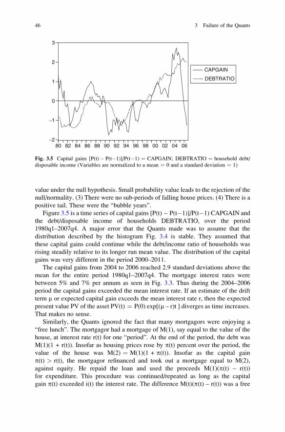
value under the null hypothesis. Small probability value leads to the rejection of the

null/normality. (3) There were no sub-periods of falling house prices. (4) There is a

positive tail. These were the “bubble years”.

Figure 3.5 is a time series of capital gains [P(t) – P(t�1)]/P(t�1) CAPGAIN and

the debt/disposable income of households DEBTRATIO, over the period

1980q1–2007q4. A major error that the Quants made was to assume that the

distribution described by the histogram Fig. 3.4 is stable. They assumed that

these capital gains could continue while the debt/income ratio of households was

rising steadily relative to its longer run mean value. The distribution of the capital

gains was very different in the period 2000–2011.

The capital gains from 2004 to 2006 reached 2.9 standard deviations above the

mean for the entire period 1980q1–2007q4. The mortgage interest rates were

between 5% and 7% per annum as seen in Fig. 3.3. Thus during the 2004–2006

period the capital gains exceeded the mean interest rate. If an estimate of the drift

term m or expected capital gain exceeds the mean interest rate r, then the expected

present value PV of the asset PV(t) ¼ P(0) exp[(m – r)t ] diverges as time increases.

That makes no sense.

Similarly, the Quants ignored the fact that many mortgagors were enjoying a

“free lunch”. The mortgagor had a mortgage of M(1), say equal to the value of the

house, at interest rate r(t) for one “period”. At the end of the period, the debt was

M(1)(1 + r(t)). Insofar as housing prices rose by p(t) percent over the period, the

value of the house was M(2) ¼ M(1)(1 + p(t)). Insofar as the capital gain

p(t) > r(t), the mortgagor refinanced and took out a mortgage equal to M(2),

against equity. He repaid the loan and used the proceeds M(1)(p(t) – r(t))

for expenditure. This procedure was continued/repeated as long as the capital

gain p(t) exceeded i(t) the interest rate. The difference M(t)(p(t) – r(t)) was a free

−2

−1

0

1

2

3

80 82 84 86 88 90 92 94 96 98 00 02 04 06

CAPGAIN

DEBTRATIO

Fig. 3.5 Capital gains [P(t) – P(t�1)]/P(t�1) ¼ CAPGAIN; DEBTRATIO ¼ household debt/

disposable income (Variables are normalized to a mean ¼ 0 and a standard deviation ¼ 1)


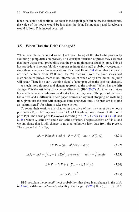
lunch that could not continue. As soon as the capital gain fell below the interest rate,

the value of the house would be less than the debt. Delinquency and foreclosure

would follow. This indeed occurred.

3.5 When Has the Drift Changed?

When the collapse occurred some Quants tried to adjust the stochastic process by

assuming a jump diffusion process. To a constant diffusion of prices they assumed

that there was a small probability that the price might take a sizeable jump. This ad

hoc procedure is not useful. How can one estimate this small probability, especially

since there were very few observations of a crisis? Figure 3.4 shows that there were

no price declines from 1980 until the 2007 crisis. From the time series and

distribution of prices, there is no information of when or by how much the jump

will occur. There is no early warning signal of a jump or when the drift has changed.

A much more rigorous and elegant approach to the problem “When has the drift

changed?” is the article by Blanchet-Scalliet et al. (Bl-S 2007). An investor divides

his wealth between a safe asset and a stock – the risky asset. The price of the stock

has a drift and a diffusion. Their paper derives an optimal stopping or switching

rule, given that the drift will change at some unknown time. The problem is to find

an “alarm signal” for when to take some action.

To relate their work to this chapter let the price of the risky asset be the house

price index P(t). The risky asset is a CDO or CDS whose price is linked to the house

price P(t). The house price Pt evolves according to (3.21), (3.22), (3.23), (3.24), and

(3.25), where mt is the drift and s dw is the diffusion. The past/current drift is m1 andwe anticipate that it will change to m2 at an unknown later date from the present.

The expected drift is Emt.

dPt ¼ Ptðmt dtþ sdwÞ P ¼ Pð0Þ dw � Nð0; dtÞ (3.21)

d ln Pt ¼ ðmt � s2=2Þdtþ sdwt (3.22)

ln Pt ¼ ln PþZ

ms � 1=2ð Þs2� �dsþ swðtÞ wðtÞ ¼

Ztdwsds (3.23)

E ln Pt ¼ ln PþZt Ems � 1=2ð Þs2� �

ds (3.24)

var ln Pt ¼ s2 t (3.25)

Bl-S postulate the unconditional probability, that there is no change in the drift,

is (3.26a), and theunconditionalprobabilityof achange is (3.26b). IfPr (mt ¼ m1) ¼0.5,

3.5 When Has the Drift Changed? 47

then the half-life in state m1 is (3.26c). Thusl > 0 is inversely related to the half – life

in state 1.

Pr ðmt ¼ e�ltÞ t � 0 (3.26a)

Pr ðmt ¼ m2Þ ¼ 1� e�lt: (3.26b)

ln ð0:5Þ=l ¼ 0:69=l ¼ half � life (3.26c)

From (3.21, 3.22, 3.23, 3.24, 3.25, 3.26) how should one determine if drift m has

changed? This is an important question since it determines the optimal ratio of risky

assets/wealth and the implied optimum growth rate of wealth.

They contrast three approaches. In one, the optimization is based upon a

misspecified model, for example where future changes are ignored. The second is

empirical. A moving average of prices is used to estimate when the drift has

changed. Chartist trading rules are just based upon the history of the asset price.

The third are two model-detect strategies.

Their model dependent optimization procedure is directly related to the question

when has the drift changed? This challenge is illustrated by Fig. 3.5 above

concerning the capital gain. I sketch the Bl-S approach.

Utility function of wealth ln X(t), implies considerable risk aversion. The aim is

to select the proportion pt in the risky asset to maximize the expected logarithm of

wealth ln X(T) to time T > 0. That is, pt maximizes (3.27).

G ðXÞ ¼ max E ln XT=X; X ¼ Xð0Þ: (3.27)

X ¼ wealth ¼ value of risky asset þ value of safe asset

Their constraint is that 1 > p > 0. Assume that m1 > r > m2. The drift starts

above the safe rate and then will fall below it at some unknown time. The question

is when one should reduce or even get out of the risky asset. When will the bubble

burst? The expected drift times the fraction of wealth in the stock is ptEmt.Using the stochastic calculus Ito equation they derive (3.28) from (3.27), (3.22)

and an equation for wealth, a linear combination of the stock and the safe asset.

ElnXT=X ¼ZT ½ptEmt � pt2s2=2�dtþ rT (3.28)

Hence the optimal proportion p*t to be held in the risky asset is (3.29).

p�t ¼ argmax½ptEmt � pt2s2=2� (3.29)

This ratio maximizes the expected utility, the expected logarithm of wealth at

time T.

Their goal is to find a stopping rule that detects at what instant t the drift of thehouse price index has changed. Since the investor observes the house price P(t), but

cannot observe the drift m(t), this is a partially observed optimal stopping problem.


A technique using nonlinear filtering formulas to reduce this partially observed

problem to a completely observed problem was first used by Shiryayev and has now

become standard. Bl-S et al compute the wealth of the trader who uses one of the

two Model and Detect Strategies, relative to the Moving Average atheoretical

approach. They ask. Is it better to invest according to mathematical Model andDetect strategy based upon a mis-specified model, or according to a strategy whichis model free?

The main mathematical tool used to obtain these two stopping rules is the

process Ft, the conditional probability that the (unknown) change point appeared

before the running time t. For each procedure, the trader decides to invest his wealth

in the risky asset when Ft differs from a given quantity defined in their paper.

The Bl-S equation (3.30) is the conditional expectation of the drift m*t. VariableFt, is the conditional probability that the change in the mean rate of return from has

occurred by time t, given the observed house prices up to that time. If F ¼ 1

then the jump down from m1 to m2 has occurred. If F ¼ 0, the jump has not yet

occurred. The mean rate of return mt is a hidden state with two possibilities, m1 or m2,Only one change in the state is allowed at an random exponentially distributed time

t. This is different from an unconditional expectation based upon (3.26a), (3.26b).

Using (3.30)

m�t ¼ ½m1 � s2=2Þ þ ðm2 � m1ÞFt� (3.30)

in (3.29), they determine the optimal ratio of the risky asset/wealth p*t whichmaximizes expected logarithm utility given the stochastic process on the drift.

The evolution of Ft, the conditional probability that change has already occurred,

is based upon a likelihood ratio and an innovation process. It depends upon both theobserved house prices and the conditional probabilities Fs, for s � t. The details

are in their article. For my purposes, the derived conditional probability has the

following characteristics [Bl-S, eqs. A6, A7].

Start with a drift m1. One has a prior and a recent sample. The forecasting error

compares the current price realization ln P(t) with what is expected from the prior

drift [m1 – s2/2]t. The difference is used to obtain the probability Ft that the change

in drift from m1 to m2 has already occurred.

They conclude (p. 1,366): “We can now address our main question: Is it better to

invest according to a mathematical Model and Detect strategy based upon a

mis-specified model or according to a strategy which is model-free? Due to the

analytical complexity of all the explicit formulae that we have obtained for the

various expected utilities of terminal wealth, we have not as yet succeeded to find a

mathematical answer to this question. . . We therefore present numerical results

obtained from Monte Carlo simulations to illustrate our comparisons.”

Bl-S simulate the models and conclude (p. 1,367) “Our numerical study suggests

that there is no universal solution to the problem of parameter mis-specification.

It seems that when the drifts are high in absolute terms and in particular, when the

upward drift is high, the performance of the Model and Detect strategies can be

3.5 When Has the Drift Changed? 49

quite robust and superior to the one of the chartist trading strategy. However, their

performance deteriorates rapidly when l is strongly mis-specified and/or when

the upward drift is not very high. Since the second drift is in fact the hardest to

estimate due to the fact that we lack a priori information, we recommend caution

before asserting that the Model and Detect strategies are superior to the technical

trading rule. Indeed the Model and Detect strategies only offer a clear comparative

advantage over the chartist trading rule in the presence of strong expected future

trends”.

3.6 Conclusion: Errors of the Quants

According to the EMH, it is impossible to know when a bubble is occurring because

current prices reflect all publicly available information. Only in retrospect, when the

bubble has collapsed, can one infer that prices did not reflect “the fundamentals”.

This was precisely Greenspan’s view (Chap. 2): the crisis was unpredictable.

The theme of this book, in chapters below, is that Greenspan was in error.

The Quants/market made three interrelated errors. First, they based the expected

house price upon the current price and drift according to (3.20). When the drift

m ¼ 0, the expected price was just the current price (EMH). A second closely

related error is that they assumed that the distribution of capital gains is constant, so

they could derive a VaR on that basis. The mistake was that the Quants ignored

publicly available information in forming expectations, as discussed in Chap. 2.

The ultimate determinant of the values of CDOs was the ability of the mortgagors to

service their debts. The income to the owners of the CDOs and their values comes

from the flow of income through the tranches starting with the mortgagors. It was

public information that the mortgages were of most dubious value, no due diligence

was performed in the ratings and the debt/income of the mortgagors –

DEBTRATIO in Fig. 3.5 was rising. Hence it was improbable that the distribution

of house prices would remain constant. This systemic risk was ignored by the

Quants who just focused upon current prices.

A third major error of the Quants was to assume the independence of the returns

to the tranches, the “apples in the basket” model, instead of the correlations in the

“slices of bread in a loaf” model.

References

Blanchet-Scalliet, C., A. Diop, R. Gibson, D. Talay, and E. Tancre. 2007. Technical analysis

compared to mathematical models based methods under parameter mis-specification. Journalof Banking and Finance 31(5): 1351–1373.

Cheng, Ren. 2009. Some reflections on the current state of financial mathematics, GraduateInternational Colloquia Grant, Challenges of Mathematical Modeling and Numerical


Computation in Finance, Division Applied Mathematics Brown University. <www.dam.

brown.edu./colloquium/DAM_colloquium/Schedule.html>.

Congressional Oversight Panel (COP). 2009. Special Report on Regulatory Reform, Washington,

DC.

Derman, Emanuel. 2004. My life as a quant. New Jersey: Wiley.

Fama, Eugene. 1970. Efficient capital markets: A review of theory and empirical work. Journal ofFinance 25(2): 383–417.

Feller, William. 1966. An introduction to probability theory and its applications II. New York:

Wiley.

Financial Crisis Inquiry Report (FCIC). 2011. Perseus Group. New York.

Fleming, Wendell, and Mete Soner. 2006. Controlled Markov processes and viscosity solutions.New York: Springer.

Patterson, Scott. 2010. The quants. New York: Crown Business.

Samuelson, Paul. 1957. Intertemporal price equilibrium: A prologue to the theory of speculation.Reprinted in Collected Papers (1966) II.

Samuelson, Paul. 1965. Proof that properly anticipated prices fluctuate randomly. Reprinted in

Collected Papers (1972), III.

Sharpe, W.F. 1964. Capital asset prices: A theory of market equilibrium under conditions of risk.

Journal of Finance 19(3): 425–442.Stein, Jerome L. 1986. The economics of futures markets. Oxford: Blackwell.Yang, Jichuan. 2009. The making of a beautiful thing, or a financial weapon of mass destruction,

Graduate International Colloquia Grant, Challenges of Mathematical Modeling and Numerical

Computation in Finance, Division Applied Mathematics Brown University. <www.dam.

brown.edu./colloquium/DAM_colloquium/Schedule.html>.

References 51

Chapter 4

Philosophy of Stochastic Optimal

Control Analysis (SOC)

Abstract I discuss the philosophy of the stochastic optimal control techniques

used in later chapters. The net worth of the real estate sector in Chap. 5, and of AIG

in Chap. 6, evolve dynamically. In the first case, debt is incurred in period t to

purchase assets whose return is uncertain, and must be repaid in period t + 1 at an

uncertain interest rate. In the second case, insurance is sold in period t and the

claims in period t + 1 are uncertain. What is the optimal debt in the first case and

what are the optimal insurance liabilities in the second case? I discuss the strengths

and limitations of alternative criterion functions, what should the firm or industry

maximize? How should risk aversion be taken into account? Then I discuss the

modeling of reasonable stochastic processes of the uncertain variables. Given the

criterion function, each stochastic process implies a different quantitative, but

similar qualitative, optimum debt/net worth or insurance liabilities/net worth.

Using SOC I derive quantitative measures of an optimal and an excessive leverage,

or what is an excessive risk that increases the probability of a crisis? The optimal

capital requirement or leverage balances risk against expected growth and return.

4.1 Why Use Stochastic Optimal Control?

Neither the markets, the IMF nor the Central Banks anticipated the US financial

crises until it was too late. The collapse of the housing market led to solvency

problems – where debt exceeded assets – and liquidity problems, where key firms in

the shadow banking system could not obtain sufficient liquid resources to service

their debts. In many cases the failures led to bailouts, discussed in subsequent

chapters. The basic question is: What is an “excessive” debt ratio for two key

sectors in the crisis: the real estate sector and a large insurer such as AIG, that is

likely to lead to a crisis? I explain why SOC is a valuable tool to derive theoretically

based, not empirical ad hoc, measures of an excess debt that will be an Early

Warning Signals (EWS) of a debt crisis.


53

Net worth is assets less debt. The crucial variable is leverage or the debt/net

worth ratio. Leverage ¼ assets/net worth ¼ 1 + debt/net worth. The growth of net

worth is affected by leverage. An increase in debt at time t to finance the purchase of

assets increases the growth of net worth by the return on investment. The return on

investment has two components. The first is the productivity of assets and the

second is the capital gain on the assets. The resulting higher debt decreases the

subsequent growth of net worth by the associated interest payments and servicing of

the debt. As a result an increase in leverage will increase expected growth of net

worth if the return on investment exceeds the interest rate on the higher debt.

The productivity of assets is observed, but the future capital gain and the interest

rates are unknown when the investment decision is made.

The basic equation for the growth of net worth is crucial to understanding

optimal risk management and evaluation of desirable policy. Two cases are

discussed in detail in the chapters below. In Chap. 5, the focus is upon the real

estate sector and the US financial crisis. In Chap. 6, the focus is upon AIG which

sold Credit Default Swaps (CDS) – a form of insurance – against the financial

derivatives that were based upon debt from the real estate market. In both cases,

I use the SOC approach.

The first case concerns the real estate market. The mortgagors/households

borrow from banks, which then package the mortgages and sell these packages to

investors. Focus upon the net worth of the mortgagors/real estate industry whose

interest payments become income to the buyers of mortgages and their derivatives.

The purchase of mortgages assets, which are investments in housing, implies a rise

in the ratio of debt/net worth of the real estate sector. The income of the financial

structure and the shadow banking system ultimately was derived from the ability of

the mortgagors to service their debts. The increase in debt would raise the growth of

net worth of the real estate sector if the capital gain on the assets – the appreciation

of house prices – plus the rate of return on the assets exceed the interest rate (4.1).

Change in net worth ¼ ½assetsðcapital gainþ productivity of assetsÞ�� interest rateðdebtÞ � ðconsumption or dividendsÞ (4.1)

The capital gains and the interest rates are described in Chap. 3. The huge capital

gains in housing and low interest rates, during the period 2002–2006 led to a rise in

the ratio debt/net worth of the real estate sector. The first term in brackets was large

so the private housing sector increased its debt directly to banks and indirectly to

foreign investors. The investment in housing seemed to be profitable because the

debt could be refinanced/repaid from the recent capital gains – not from the produc-

tivity of assets/the “marginal product of capital”. Those capital gains were not

sustainable. The reason is that insofar as the capital gain exceeds the appropriate

interest rate, the present value of the asset diverges to infinity.

There is a dynamic process. Borrowing to purchase assets in period t has a return.

The value of assets changes, resulting from the capital gain (or loss). At time

(t + dt) the unit has a greater debt that must be serviced. The higher debt raises

54 4 Philosophy of Stochastic Optimal Control Analysis (SOC)

the term [(interest rate) (debt)] in period (t + dt), which tends to lower the growth of

net worth. Actions taken at time t have consequences at time (t + dt). The risk is

that with the higher debt ratios, there would be a period when the capital gains fell

below the interest rate – such as occurred in 2007–2008. In fact the capital gain term

and interest rate term are negatively correlated. When interest rates declined, house

prices rose – the boom/bubble. When interest rates rose, capital gains declined.

When the growth of housing prices declined, then the large negative term – the

return less the interest rate – is multiplied by a large debt ratio and the net worth of

the housing industry vanishes. The housing sector defaults on their loans. Bank

failures followed the collapse of the housing market. The government then

intervened to avert the collapse of the financial system. The question is what is an

optimal debt/net worth ratio at any time? How should one judge if the debt and risk

were too large? The techniques of SOC are used in Chap. 5 to answer this question.

The second case concerning AIG is discussed in Chap. 6. The AIG Financial

Products AIGFP subsidiary of AIG sold credit default swaps (CDSs) involving

three parties. Party 1 the obligor sells the “reference securities” to party 2. The latter

are security houses, hedge funds that purchase protection from party 3, who are

banks and insurance companies, which issue the protection. In many cases

municipalities are required to carry insurance in order to market their bonds, or to

obtain a high credit rating. The CDSs are privately negotiated contracts that

function in a similar manner to insurance contacts, but their payoff structure is

closer to a put option. The CDS liability requires that the insurer pay, or put up more

collateral, if the market value of the securities insured falls below the notional

amount insured. Surplus is the difference between assets and liabilities less initial

contributed capital. The change in surplus is the sum of several components (4.2).

Change in surplus ¼ ðpremium rateÞ liabilitiesþ ðreturnþ capital gainÞ assets� ðclaims on the company related to liabilitiesÞ (4.2)

The insurer incurs a liability at time t, and receives a premium for the amount

insured. This increases assets and surplus at time t. The capital gain (or loss) and

claims at time t + dt are unknown at time t when the insurance is sold. The surplus

at time t + dt rises as a result of the return, equal to the productivity plus the capital

gain on assets. Surplus declines by the amount of claims at time t + dt against

liabilities incurred earlier.

The stochastic variables are the capital gains on assets and claims against the

insurer. They are unknown at time t when the liabilities are incurred. The control

variable of the insurance company is its liabilities, the insurance policies sold such

as CDS. The question is: what is the optimum amount of insurance liabilities?

When should the firm and/or regulators decide that liabilities are too large?

In (4.1) the control variable is the debt of the real estate sector and in (4.2) it is

the liabilities of the insurer. The capital gains, interest rate or claims in the cases

above are subject to imperfectly known disturbances that may be taken as random.

Stochastic optimal control theory attempts to deal with models in which random

4.1 Why Use Stochastic Optimal Control? 55

disturbances are very important. I deal with the case where the controller knows the

state of the system at each time t. In deterministic systems, if one knows the initial

conditions, the model and controls, then the paths of the variables can be predicted

perfectly. For stochastic systems, it is completely different. There are many paths

that the system may follow from the controls and initial data. In the stochastic case,

the best system performance depends on the information available to the controller

at each time t. The method of dynamic programming is generally used. The basic

references for techniques used in this approach are: Fleming–Rishel, Chaps. V and

VI, Fleming–Soner, Fleming–Stein (2004) and Stein (2005).

4.2 Research Strategy

My research strategy parallels the views of Fischer Black and Emanuel Derman

(2004, ch. 16). I paraphrase/quote their views. Certain economic quantities are so

hard to estimate that Black called them “unobservables”. One unobservable is

expected return. So much of finance deals with this quantity unquestioningly.

Yet our estimates of expected return are so poor, that Black said that they are

almost laughable.

The Value at Risk VaR uses statistical distributions to assign probabilities of the

firm’s value into the future, and statistics are inevitably based upon the past. But

VaR is too simplistic. The statistical distributions are not necessarily stationary.

The past does not repeat itself. People learn from experience, which subsequently

changes the distributions. We are ignorant of the true probabilities – the extreme

tails of price distributions.

Black described the approach of the finance profession as follows: “In the

end a theory is accepted not because it is confirmed by conventional empirical

tests, but because researchers persuade one another that the theory is correct and

relevant”. This “group think” behavior led to serious consequences as described in

Chaps. 2 and 3.

The question is what is the “right model” to analyze problems posed in Sect. 4.1

above? The Quants are physicists, mathematicians and computer scientists who do

“financial engineering”. They apply models from physics to the world of finance.

Derman has moved between the world of Wall St. Quants and academia. He wrote

that models in finance differ from those in physics. “Models are only models, not

the thing in itself. We cannot therefore expect them to be truly right. Models are

better regarded as a collection of parallel thought universes you can explore. Each

universe should be consistent, but the actual financial and human world, unlike the

world of matter, is going to be infinitely more complex than any model we make of

it. We are always trying to shoehorn the real world into one of the models to see

how useful approximation it is”.

His strategy, which I follow, can be summarized. One must ask: Does the model

give you a set of plausible variables to describe the world, and a set of relationships

between them that permits its analysis and investigation. The real question is how


useful is the theory? “The right way to engage with a model is, like a fiction reader

or a really great pretender, to temporarily suspend disbelief, and then push it as

far as possible”.

For these reasons, I consider a set of plausible models and derive the optimal

controls, debt ratio or liability ratio, using SOC. Call the optimal ratio f*(t), which

varies quantitatively among models. I then consider an upper bound on the optimal

control for both models and call it f**(t). I compare the actual debt ratio or liability

ratio, called f(t), with this upper bound. Thereby, I derive a measure of “excess

debt” C(t) ¼ [f(t) � f**(t)], the actual less upper bound optimal. I explain that the

probability of a debt crisis is directly related toC(t) the excess debt. On the basis of

this measure of excess debt, I derive early warning signals of the US financial crisis

of 2008 and the debt crises of the 1980s.

4.3 Modeling the Uncertainty, the Stochastic Variables

In general, focus upon the change in net worth (4.1). It can be written as (4.3).

dXðtÞ ¼ XðtÞ½ð1þ f ðtÞÞ ðdPðtÞ=PðtÞ þ bðtÞdtÞ � iðtÞf ðtÞ � c dt� (4.3)

X(t) ¼ Net worth, f(t) ¼ debt/net worth ¼ L(t)/X(t), dP(t)/P(t) ¼ capital gain

or loss, i(t) ¼ interest rate, (1 + f(t)) ¼ assets/net worth, b(t) ¼ productivity of

capital. C(t)/X(t) ¼ c (t) ¼ consumption/net worth ¼ c is taken as given.

The sources of uncertainty are dP(t)/P(t) the capital gain or loss, and i(t)

the interest rate. How should the stochastic variables be modeled? I consider

in the chapters below two models that differ in their assumptions about the

stochastic processes.

In Model I, assume that the price grows at a trend rate and there is a deviation

from the trend. The deviation from trend is a stochastic variable that has two parts.

The first part converges to zero and the second is random with a mean of zero and a

positive finite variance. This deviation is an Ornstein Uhlenbeck ergodic mean

reverting process. This implies a stochastic differential equation for the capital

gains term. The interest rate has two parts, a constant mean plus a diffusion or

random term, with a zero mean and finite variance. The capital gains term and

interest rate are negatively correlated. Declines in interest rates lead to capital gains,

and rises in interest rates lead to capital losses.

Since the growth of net worth equation (4.3) will differ according to the model

assumed, the derived optimal debt ratio will differ in the two models. I examine the

empirical data to decide which assumption is to be preferred. However, the tests do

not allow one to reject either hypothesis.

Model II considers the return capital, the capital gain plus the productivity of

capital, b(t) to be a stochastic variable. There are two parts to the return b(t). One is

the mean b dt and the second is a diffusion sb dwb. The interest rate has a mean i dt

and a diffusion si dwi the latter is a random variable with a zero expectation.

4.3 Modeling the Uncertainty, the Stochastic Variables 57

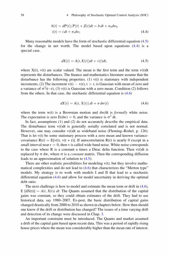
bðtÞ ¼ dPðtÞ=PðtÞ þ bðtÞdt ¼ b dtþ sbdwb

iðtÞ ¼ i dtþ sidwi (4.4)

Many reasonable models have the form of stochastic differential equation (4.5)

for the change in net worth. The model based upon equations (4.4) is a

special case.

dXðtÞ ¼ Aðt;XðtÞÞdtþ vðtÞdt; (4.5)

where X(t), v(t) are scalar valued. The mean is the first term and the term v(t)dt

represents the disturbances. The finance and mathematics literature assume that the

disturbance has the following properties. (1) v(t) is stationary with independent

increments, (2) The increment v(t) � v(r), t > r, is Gaussian with mean of zero and

a variance of s2(t�r), (3) v(t) is Gaussian with a zero mean. Condition (2) follows

from the others. In that case, the stochastic differential equation is (4.6)

dXðtÞ ¼ Aðt; XðtÞÞ dtþ s dwðtÞ (4.6)

where the term w(t) is a Brownian motion and dw/dt is formally white noise.

The expectation is zero E(dw) ¼ 0, and the variance is s2 dt.

In fact, assumptions (1) and (2) do not accurately describe the empirical data.

The disturbance term v(t)dt is generally serially correlated and is not normal.

However, one may consider v(t)dt as wideband noise (Fleming–Rishel, p. 126).

That is let v(t) be some stationary process with a zero mean and known variance-

covariance R(r) ¼ E[v(t), v(t + r)]. If autocorrelation R(r) is nearly 0 except in a

small interval near r ¼ 0, then v is called wide band noise. White noise corresponds

to the case where R is a constant a times a Dirac delta function. Then v(t)dt is

replaced by s dw, where s is a constant matrix. Then the corresponding diffusion

leads to an approximation of solution to (4.5).

There are other realistic possibilities for modeling v(t), but they involve mathe-

matical complexities and do not lead to (4.6) that characterizes the “Merton type”

models. My strategy is to work with models I and II that lead to a stochastic

differential equation (4.6) and allow for model uncertainty in deriving the optimal

debt ratio.

The next challenge is how to model and estimate the mean term or drift in (4.6),

E [dX(t)] ¼ A(t, X(t)) dt. The Quants assumed that the distribution of the capital

gains was constant, so they could obtain estimates of the drift. They had to use

historical data, say 1980–2007. Ex-post, the basic distribution of capital gains

changed drastically from 2000 to 2010 as shown in chapters below. How then should

one know if the drift or distribution has changed? The issues of a time varying drift

and detection of its change were discussed in Chap. 3.

An important constraint must be introduced. The Quants and market assumed

a drift of the capital gain based upon recent data. This was a period of rapidly rising

house prices where the mean was considerably higher than the mean rate of interest.


Mortgagors refinanced their homes and incurred a debt equal to the current high

house prices. The latter exceeded the value of the initial mortgage. They consumed

the monetary difference between the value of the new loan and the value of the old

loan. In the next period, insofar as the house price appreciated at a greater rate than

the interest rate, they were able to repeat the process: refinance and consume

the difference between the value of the home and the new debt. This was a free

lunch. The mortgagor may have been a NINJA (no income, no job, no assets) and

the loan originator did not worry for two reasons. First, the equity in the home

was rising due to the capital gain. Second, the originator sold the mortgages

that were then packaged and sold to investors. Free lunches cannot continue.

I therefore constrain the optimization: the drift of the capital gain should not exceed

the mean rate of interest.

4.4 Criterion Function

Chapters 2 and 3 explained that the finance industry has been poor at risk manage-

ment and that the regulators have been ineffective. I assume that there is a

hypothetical or ideal optimizer. In the financial market case it is the real estate

industry. In the insurance case it is AIG. In each case the hypothetical optimizer

selects a debt ratio that maximizes the expectation of a concave function of net

worth Max EU(X(T)) at a terminal date T, subject to dynamic stochastic processes.

This is a benchmark for optimality.

The criterion function should satisfy several requirements. (1) Losses are

penalized more than equal gains are rewarded. This requirement seems to have

been ignored or reversed in the finance industry/Wall St. prior to the crisis.

What the market seemed to optimize differed from the requirements of an “opti-

mal” solution. (2) Very low values of X(T) should be very severely penalized.

This too was ignored due to the moral hazard where major firms anticipated that a

friendly Treasury/Federal Reserve would bail out “too big to fail” firms.

In modeling, the distribution of the stochastic variable in (4.6) is assumed to be

normal, but in reality it is not. There may be a fat tail, where there is a low

probability of very large losses. Large losses may not be likely, but they should

get very heavy weights in the criterion/utility function.

Utility U(X-Y) is (4.7), using a second order approximation around U(X) for

small values of stochastic variable Y. It has a zero mean and a variance of s2

UðX � YÞ ¼ UðXÞ � U0ðXÞY þ ð1=2ÞU00ðXÞY2 (4.7)

E(Y) ¼ 0: (4.8)

E(Y2Þ¼ s2: (4.9)

4.4 Criterion Function 59

The expected utility is (4.10). Divide by U0(X) 6¼ 0 and assume that E(Y) ¼ 0.

Therefore (4.11) follows.

E½UðX � YÞ� ¼ UðXÞ � U0ðXÞEðYÞ þ ð1=2ÞðU00ðXÞÞEðY2Þ (4.10)

fE½UðX � YÞ� � UðXÞg=U0ðXÞ ¼ ð1=2Þ½U’’ðXÞ=U’ðXÞ�EðY2Þ (4.11)

The loss of utility due to the probability of losses depends upon risk aversion

U00(x)/U0(x), and risk s2. When U00(X)/U0(X) is significantly negative, even if E(Y)

is very small the variance imposes a large penalty.

RiskAversion¼� U’’(X)/U’(X)¼ the price onewould pay for certainty: (4.12)

There are many criterion functions that satisfy these requirements. Only a few

can be solved analytically in the optimization process. The others must be calcu-

lated numerically. In Table 4.1 I consider three widely used functions. The first is

often called HARA. The second is a logarithmic function, which is a special case of

HARA when g ¼ 0. The third is an exponential function.

These functions are different. In the HARA and exponential cases, values of X

approaching zero are not severely penalized U(0) ¼ 0. In the logarithmic case, low

values of X(T) are very severely penalized. In the HARA and logarithmic cases, the

risk aversion coefficient in column three depends negatively upon net worth. In the

exponential case, it is independent of net worth.

There are several great advantages to using the logarithmic criterion function.

First, in all cases one can derive the stochastic optimal control (SOC) – debt or

liability ratio – by using dynamic programming. However, in the logarithmic case,

the SOC can be derived directly by integrating the Ito equation. Second, a Mean-

Variance interpretation can be given to the determination of the optimal control, as I

show later in this chapter. Third, the risk coefficients either g or a are arbitrary.

Specifically, suppose that the debtor has a low risk aversion, (1 � g) is close to zeroin the HARA case. His optimum debt ratio would be very high, close to risk

neutrality. In the LTCM case, the market view was that LTCM “ran in front of

bulldozers to pick up nickels”. The lender is unlikely to be risk neutral. He may

have a very high risk aversion, and be reluctant to accommodate the borrower’s

desired debt. So the choice of g or a is arbitrary. There is a way to cope with this

problem (Stein 2007) in a general equilibrium framework, where the rate of interest

equilibrates the demand and supply of debt.

Table 4.1 Alternative criteria/utility functions

Criterion function

U(X(T))

Lim X(T) as

X ¼ > 0

Risk aversion coefficient

U00(X)/U0(X)(1/g)X(T)g, 1 > g 6¼ 0 0 �(1 � g)/Xln X(T) �1 �1/X

1�exp(�aX(T)) 0 �a


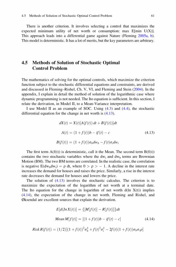
There is another criterion. It involves selecting a control that maximizes the

expected minimum utility of net worth or consumption: max E[min U(X)].

This approach leads into a differential game against Nature (Fleming 2005a, b).

This model is deterministic. It has a lot of merits, but the key parameters are arbitrary.

4.5 Methods of Solution of Stochastic Optimal

Control Problem

The mathematics of solving for the optimal controls, which maximize the criterion

function subject to the stochastic differential equations and constraints, are derived

and discussed in Fleming–Rishel, Ch. V, VI, and Fleming and Stein (2004). In the

appendix, I explain in detail the method of solution of the logarithmic case where

dynamic programming is not needed. The Ito equation is sufficient. In this section, I

relate the derivation, in Model II, to a Mean-Variance interpretation.

I use Model II as an example of SOC. Using (4.3) and (4.4), the stochastic

differential equation for the change in net worth is (4.13).

dXðtÞ ¼ XðtÞ½Aðf ðtÞÞ dtþ Bðf ðtÞÞ�dt

AðtÞ ¼ ð1þ f ðtÞÞb� if ðtÞ � c (4.13)

Bðf ðtÞÞ ¼ ð1þ f ðtÞÞsbdwb � f ðtÞsidwi

The first term A(f(t)) is deterministic, call it the Mean. The second term B(f(t))

contains the two stochastic variables where the dwi and dwb terms are Brownian

Motion (BM). The two BM terms are correlated. In the realistic case, the correlation

is negative E(dwbdwi) ¼ r dt, where 0 > r > � 1. A decline in the interest rate

increases the demand for houses and raises the price. Similarly, a rise in the interest

rate decreases the demand for houses and lowers the price.

The solution of (4.13) involves the stochastic calculus. The criterion is to

maximize the expectation of the logarithm of net worth at a terminal date.

The Ito equation for the change in logarithm of net worth d(ln X(t)) implies

(4.14), the expectation of the change in net worth. Fleming and Rishel, and

Øksendal are excellent sources that explain the derivation.

E½dðIn XðtÞÞ� ¼ f½M½ f ðtÞ� � R½ f ðtÞ��gdt

MeanM½ f ðtÞ� ¼ ½ð1þ f ðtÞÞb� if ðtÞ � c� (4.14)

Risk Rðf ðtÞÞ ¼ ð1=2Þ½ð1þ f ðtÞÞ2s2b þ f ðtÞ2s2i � 2f ðtÞð1þ f ðtÞÞsbsir�

4.5 Methods of Solution of Stochastic Optimal Control Problem 61

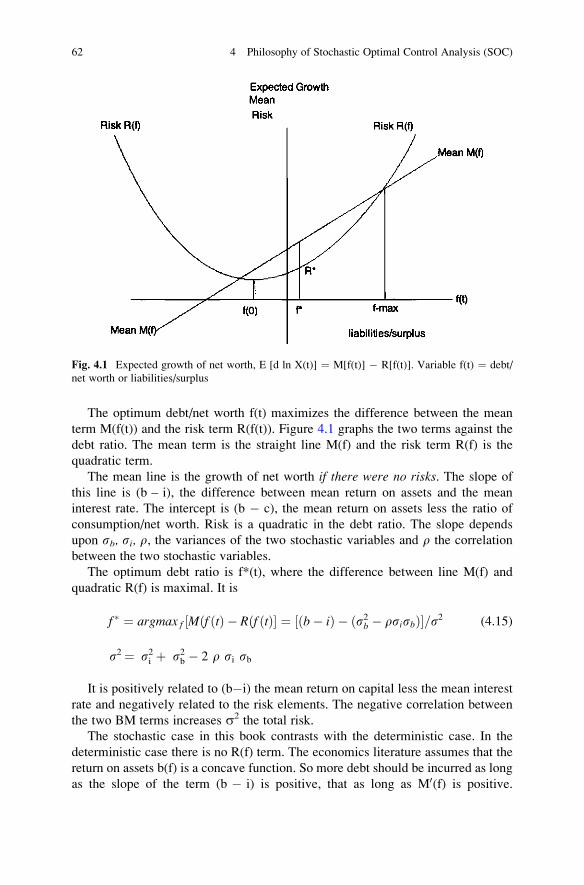
The optimum debt/net worth f(t) maximizes the difference between the mean

term M(f(t)) and the risk term R(f(t)). Figure 4.1 graphs the two terms against the

debt ratio. The mean term is the straight line M(f) and the risk term R(f) is the

quadratic term.

The mean line is the growth of net worth if there were no risks. The slope of

this line is (b – i), the difference between mean return on assets and the mean

interest rate. The intercept is (b � c), the mean return on assets less the ratio of

consumption/net worth. Risk is a quadratic in the debt ratio. The slope depends

upon sb, si, r, the variances of the two stochastic variables and r the correlation

between the two stochastic variables.

The optimum debt ratio is f*(t), where the difference between line M(f) and

quadratic R(f) is maximal. It is

f � ¼ argmax f ½Mðf ðtÞ � Rðf ðtÞ� ¼ ½ðb� iÞ � ðs2b � rsisbÞ�=s2 (4.15)

s2 ¼ s2i þ s2b � 2 r si sb

It is positively related to (b�i) the mean return on capital less the mean interest

rate and negatively related to the risk elements. The negative correlation between

the two BM terms increases s2 the total risk.

The stochastic case in this book contrasts with the deterministic case. In the

deterministic case there is no R(f) term. The economics literature assumes that the

return on assets b(f) is a concave function. So more debt should be incurred as long

as the slope of the term (b � i) is positive, that as long as M0(f) is positive.

Fig. 4.1 Expected growth of net worth, E [d ln X(t)] ¼ M[f(t)] � R[f(t)]. Variable f(t) ¼ debt/

net worth or liabilities/surplus


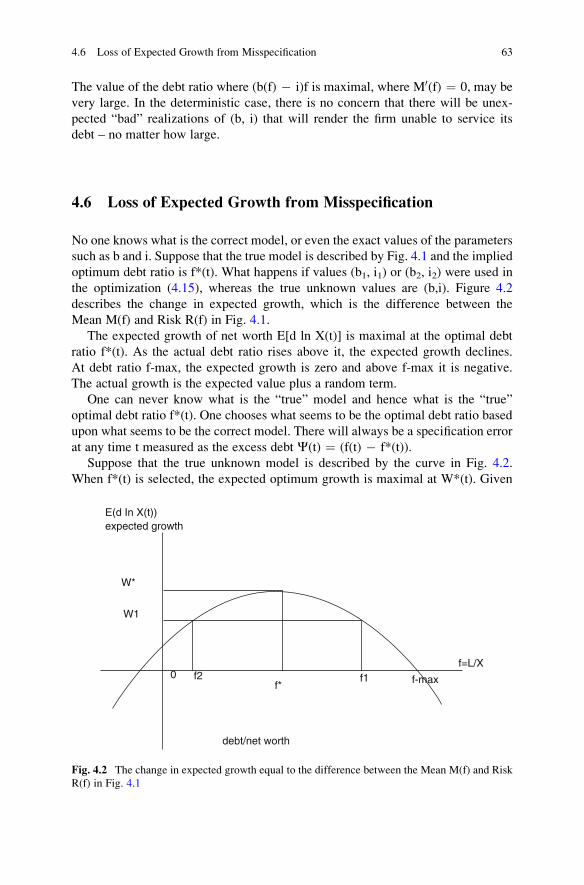
The value of the debt ratio where (b(f) � i)f is maximal, where M0(f) ¼ 0, may be

very large. In the deterministic case, there is no concern that there will be unex-

pected “bad” realizations of (b, i) that will render the firm unable to service its

debt – no matter how large.

4.6 Loss of Expected Growth from Misspecification

No one knows what is the correct model, or even the exact values of the parameters

such as b and i. Suppose that the true model is described by Fig. 4.1 and the implied

optimum debt ratio is f*(t). What happens if values (b1, i1) or (b2, i2) were used in

the optimization (4.15), whereas the true unknown values are (b,i). Figure 4.2

describes the change in expected growth, which is the difference between the

Mean M(f) and Risk R(f) in Fig. 4.1.

The expected growth of net worth E[d ln X(t)] is maximal at the optimal debt

ratio f*(t). As the actual debt ratio rises above it, the expected growth declines.

At debt ratio f-max, the expected growth is zero and above f-max it is negative.

The actual growth is the expected value plus a random term.

One can never know what is the “true” model and hence what is the “true”

optimal debt ratio f*(t). One chooses what seems to be the optimal debt ratio based

upon what seems to be the correct model. There will always be a specification error

at any time t measured as the excess debt C(t) ¼ (f(t) � f*(t)).

Suppose that the true unknown model is described by the curve in Fig. 4.2.

When f*(t) is selected, the expected optimum growth is maximal at W*(t). Given

expected growthE(d In X(t))

W*

W1

0 f2f*

debt/net worth

f1f=L/X

f-max

Fig. 4.2 The change in expected growth equal to the difference between the Mean M(f) and Risk

R(f) in Fig. 4.1

4.6 Loss of Expected Growth from Misspecification 63

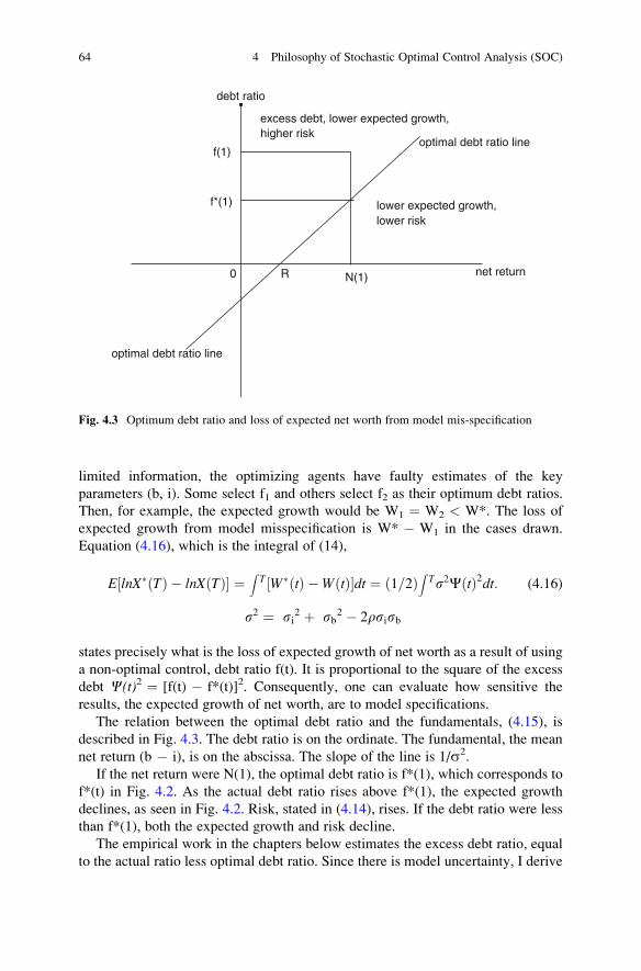
limited information, the optimizing agents have faulty estimates of the key

parameters (b, i). Some select f1 and others select f2 as their optimum debt ratios.

Then, for example, the expected growth would be W1 ¼ W2 < W*. The loss of

expected growth from model misspecification is W* � W1 in the cases drawn.

Equation (4.16), which is the integral of (14),

E lnX�ðTÞ � lnXðTÞ½ � ¼Z

T W�ðtÞ �WðtÞ½ �dt ¼ 1=2ð ÞZ

Ts2CðtÞ2dt: (4.16)

s2 ¼ si2 þ sb2 � 2rsisb

states precisely what is the loss of expected growth of net worth as a result of using

a non-optimal control, debt ratio f(t). It is proportional to the square of the excess

debt C(t)2 ¼ [f(t) � f*(t)]2. Consequently, one can evaluate how sensitive the

results, the expected growth of net worth, are to model specifications.

The relation between the optimal debt ratio and the fundamentals, (4.15), is

described in Fig. 4.3. The debt ratio is on the ordinate. The fundamental, the mean

net return (b � i), is on the abscissa. The slope of the line is 1/s2.

If the net return were N(1), the optimal debt ratio is f*(1), which corresponds to

f*(t) in Fig. 4.2. As the actual debt ratio rises above f*(1), the expected growth

declines, as seen in Fig. 4.2. Risk, stated in (4.14), rises. If the debt ratio were less

than f*(1), both the expected growth and risk decline.

The empirical work in the chapters below estimates the excess debt ratio, equal

to the actual ratio less optimal debt ratio. Since there is model uncertainty, I derive

excess debt, lower expected growth,higher risk

debt ratio

optimal debt ratio line

lower expected growth,lower risk

net return

optimal debt ratio line

f(1)

f*(1)

0 R N(1)

Fig. 4.3 Optimum debt ratio and loss of expected net worth from model mis-specification


an upper bound for the optimal ratio called f**(t), and calculate an excess debt as

C(t) ¼ [f(t) � f**(t)]. Then, on the basis of Fig. 4.2, the probability of a debt crisis

is directly related to C(t).

The upper bound f**(t), discussed in Chap. 5, assumes in Model I that the

mean interest rate is equal to the trend rate of growth of the price and there is no

deviation of the price from trend. In Model II the upper bound f**(t) assumes that

(b � i) ¼ b(t) the productivity of capital.

4.7 Insurance

4.7.1 Cramer-Lundberg

In the AIG case, the question is how to estimate the optimal amount of insurance

to offer. I follow Volchan’s (2007) exposition and use his notation. He writes

that the Cramer/Lundberg (C-L) model is still a landmark of non-life insurance

mathematics. It is to actuarial science what the Black-Scholes-Merton model is to

finance. The decision process concerns the amount of reserve capital that the

insurance company should keep in order to absorb the impact of possible losses

due to adverse changes in value of claims. The basic equation is (4.17), used

in all variants.

Change in surplus ¼ premium rateð Þliabilities þ returnþ capital gainð Þassets� claims on the company related to liabilitiesð Þ

(4.17)

The C-L model and its variants are concerned with the ruin problem, to be

discussed below. In (4.18), U(t) is the surplus, equal to initial capital u, plus total

premium income P(t) less aggregate claims S(t). The deterministic total of pre-

mium income P(t) in (4.19) is the product of premium rate c > 0 and time t.

The aggregate claims S(t) is the sum of Xk(t), amounts to be paid out in the period

(4.20). The number of claims arriving in the interval (0,t) is N(t).

UðtÞ ¼ uþPðtÞ � SðtÞ (4.18)

PðtÞ ¼ ct: (4.19)

SðtÞ ¼X

XkðtÞ; k ¼ 0; 1; . . .NðtÞ: (4.20)

The crucial assumption of the C-L model is that the claim number process {N(t)}

is a homogeneous Poisson process equation (4.21). This implies that the probability

that k claims will arrive in the interval is Poisson distributed. Thus P(0, lt) ¼ e�lt is

4.7 Insurance 65

the probability of no claims arriving during the interval of length t. The aggregate

claims {S(t)} is a compound Poisson process described by

P ðNðtÞ ¼ kf g ¼ e�ltðltÞk=k! (4.21)

The focus is upon (4.22) the probability Y(t) of bankruptcy/insolvency, that the

surplus at time t will be non-positive.

YðtÞ ¼ P UðtÞ � u< 0½ �; for some t> 0: (4.22)

The solution has the following characteristics. Using the above equations

the expected value of the surplus [EU(t) � u] is (4.23). The expected number of

claims E[N(t)] ¼ lt and m is the average cost per claim. Total premiums are ct.

The net profit condition is that (c � lm) > 0, the premium must exceed the average

total claim.

E UðtÞ½ � � u ¼ ct� mE NðtÞ½ � ¼ tðc� lmÞ: (4.23)

Even though the premium c > lm, the process of U(t) can attain negative

values in some subperiods. So it is important to have at least an estimate of

Y(t) ¼ P[U(t) � u] < 0 guaranteeing that it is sufficiently small.

The Cramer-Lundberg analysis is inadequate to evaluate the risk/return in the

AIG case. First, the asset side of the equation for the change in surplus is ignored.

The insurance company has assets against the liabilities that bring in income.

This is the second term in (4.17). Second, the value of the claims against AIG are

highly negatively correlated with the value of the assets. When the market value of

the insured assets decline, AIG must either compensate the insurer for the differ-

ence or put up more collateral. Third, the assets that are insured by AIG are quite

closely correlated with the assets in AIG’s portfolio.

4.7.2 Ruin Analysis

The C-L model is closely related to the Ruin problems in the probability literature.

See Feller I, II. The ruin literature is concerned with the question, what is the

probability that a firm that starts with a capital z will ultimately be ruined? Thereby

one has a framework to determine “optimal” capital.

The structure of the Ruin model is simple. In each period, a firm with a capital

of z can either gain $k with probability 1 > p > 0, or lose k with probability

q ¼ 1�p. Say that the firm has borrowed $a. If the capital falls to zero, the firm

is bankrupt: the probability of ruin is then one. If the capital rises to $a, the

probability of ruin is zero. The firm repays its debt and the story can start over.


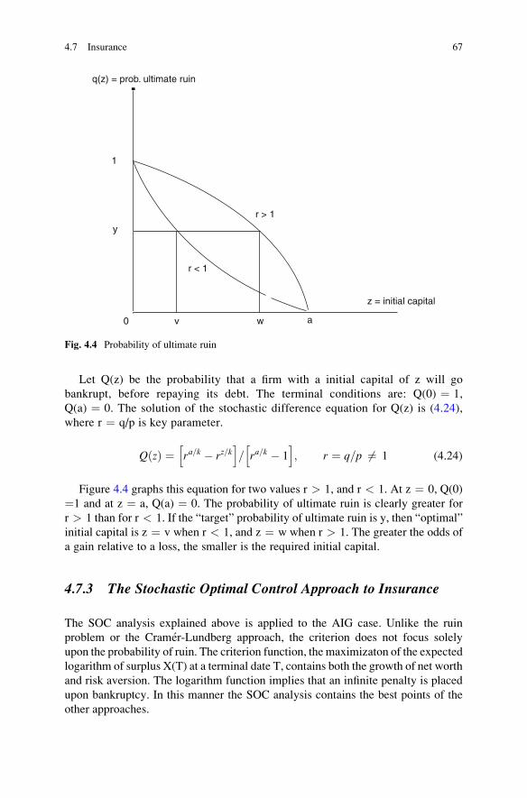
Let Q(z) be the probability that a firm with a initial capital of z will go

bankrupt, before repaying its debt. The terminal conditions are: Q(0) ¼ 1,

Q(a) ¼ 0. The solution of the stochastic difference equation for Q(z) is (4.24),

where r ¼ q/p is key parameter.

QðzÞ ¼ ra=k � rz=kh i

= ra=k � 1h i

; r ¼ q=p 6¼ 1 (4.24)

Figure 4.4 graphs this equation for two values r > 1, and r < 1. At z ¼ 0, Q(0)

¼1 and at z ¼ a, Q(a) ¼ 0. The probability of ultimate ruin is clearly greater for

r > 1 than for r < 1. If the “target” probability of ultimate ruin is y, then “optimal”

initial capital is z ¼ v when r < 1, and z ¼ w when r > 1. The greater the odds of

a gain relative to a loss, the smaller is the required initial capital.

4.7.3 The Stochastic Optimal Control Approach to Insurance

The SOC analysis explained above is applied to the AIG case. Unlike the ruin

problem or the Cramer-Lundberg approach, the criterion does not focus solely

upon the probability of ruin. The criterion function, the maximizaton of the expected

logarithm of surplus X(T) at a terminal date T, contains both the growth of net worth

and risk aversion. The logarithm function implies that an infinite penalty is placed

upon bankruptcy. In this manner the SOC analysis contains the best points of the

other approaches.

q(z) = prob. ultimate ruin

1

y

0 v

r < 1

r > 1

w a

z = initial capital

Fig. 4.4 Probability of ultimate ruin

4.7 Insurance 67

The dynamics of the process to derive E[ln X(T)] is based upon (4.25). There are

several possibilities for modeling the stochastic processes for the claims C(t) and

capital gains dP(t)/P(t). Assets ¼ A(t). Insurance liabilities ¼ L(t).

dXðtÞ ¼ pLðtÞdtþ bAðtÞdt½ � þ ðdPðtÞ=PðtÞÞAðtÞ½ � � CðtÞ: (4.25)

Assume, for simplicity, that the premium rate p is given. At this premium rate

there is an elastic demand for insurance and the insurer decides how much insur-

ance L(t) to offer at that rate. Income from premiums is p L(t)dt. The insurer has

A(t) of assets whose value is very closely related to the assets that it has insured, the

CDOs in particular. The return on these assets has two parts, a rate of return b that is

deterministic and a future capital gain or loss (dP(t)/P(t))A(t) that is unknown. Themost important stochastic variable is C(t), the future claims against the insurer

against the liabilities – insurance policies.

The modeling consists of specifying the stochastic processes on the capital

gain and the claims. Let the claims C(t) be described by stochastic differential

equation (4.26). They are proportional to L(t) the amount of insurance liabilities.

Claims are the required payments to the insured holders of CDS, due to either

defaults of the obligors or for collateral calls when the prices of the insured

securities decline. The latter led to the downfall of AIG. The mean of claims C(t)

is cL(t)dt. The variance of the claims is sc2L2(t) dt. Brownian Motion term dwc has

independent and stationary increments, with zero expectations, as assumed in the

classical literature.

CðtÞ ¼ ½cdtþ scdwc�LðtÞ:E dwcð Þ ¼ 0;E dwcð Þ2 ¼ dt:

(4.26)

Stochastic differential equation (4.27) concerns the capital gain/loss term

dP(t)/P(t). The time varying drift is a(t)dt and the diffusion is spdwp. This is a

general formulation. Models 1 and 2 of the asset price or capital gain, discussed

above, imply different values of the drift a(t). The variance of the capital gain is

sp2 dt. The dwp term has independent and stationary increments.

dPðtÞ=PðtÞ ¼ aðtÞdtþ spdwp

E dwp

� � ¼ 0; E dwp

� �2 ¼ dt:(4.27)

The two Brownian motion terms are expected to be negatively correlated (4.28):

correlation coefficient �1 � r < 0. When there is a period with capital losses

dP(t)/P(t) < 0, then claims against AIG including collateral calls are most likely

to be high. This condition accurately described the period of the AIG crisis with

CDS in Chap. 6.

E dwpdwc

� � ¼ r dt: � 1� r< 0 (4.28)


Using (4.26), (4.27), and (4.28) in (4.25), derive the stochastic differential

equation (4.29) for the change in surplus dX(t). The first set of brackets contains

the deterministic part and the second set contains the stochastic part.

dXðtÞ ¼ ½pLðtÞ þ bAðtÞ � cLðtÞ þ AðtÞaðtÞ dtþ� ½AðtÞspdwp � LðtÞscdwc�: (4.29)

X ¼ A-L ¼ surplus, A ¼ assets, L ¼ insurance liabilties, b ¼ return on assets,

p ¼ premium rate, C ¼ claims, a(t) ¼ drift capital gain, stochastic BM terms dwp,

dwc. Correlation between them is r < 0. Leverage ¼ A/X ¼ (1 + f), debt ratio

f ¼ L/X.

The SOC analysis follows very closely to what was done in Sects. 4.5 and 4.6

above. The optimal ratio of insurance liabilties/surplus f*(t) is (4.30).

f �ðtÞ ¼ p� cð Þ þ bþ aðtÞð Þ½ � � s2p � rspsc� �

= s2p þ s2c � 2rspsc� �

(4.30)

The first term in brackets in (4.30) for the optimum ratio is (p � c) the premium

less the drift of the claims plus (b + a(t)) the sum of the rate of return on assets plus

the time varying drift of the capital gain. The second term and the denominator

involve the risks of the capital gains and claims. The negative correlation between

the capital gain and the claims increases total risk and reduces the optimal ratio of

insurance liabilities/surplus.

Figures 4.1, 4.2, and 4.3 describing the determination of the loss of growth from

model misspecification and the relation between the net return and the optimal ratio

apply equally here for the optimal insurance/surplus.

AIGFP relied on Gorton’s actuarial model that did not provide a tool for

monitoring the CDO’s market value. Gorton’s model (FCIC, p. 267) had deter-

mined with 99.85% confidence that the owners of super-senior tranches of the

CDO’s insured by AIGFP would never suffer real economic losses. The company’s

auditor PWC apparently was also not aware of the collateral requirements. PWC

concluded that “..the risk of default on the [AIG] portfolio has been effectively

removed as a result of a risk management perspective. . .”.The SOC analysis leads to a very different way of viewing AIG risk than was

used by Gorton and the company’s auditor PWC.

4.8 The Endogenous Changing Distributions

Underlying all dynamic optimizations is the characterization of the price

distributions. The usual assumptions are that the system parameters are unchanging.

Ren Cheng (Fidelity Investments) gave an insightful presentation of the limitations

of the existing approaches used in financial modeling. I conclude this chapter with a

discussion of Cheng’s presentation.

The finance models assume that the means-variances-covariances are stable.

Each entity in the optimization is considered in isolation. There is no consideration

of a feedback among units, or the global effects of the collective action upon the

4.8 The Endogenous Changing Distributions 69

distribution functions. The latter are assumed to be normal, an assumption justified

by the Central Limit Theorem (CLT). We know a lot about the decision making

process of an individual unit in portfolio optimization. But we are ignorant of how

the units interact and thereby change the distributions. In Chaps. 5 and 6, I explain

how the interactions among units in the shadow banking system magnified the

collapse of housing prices upon the financial system. The whole was much greater

than the sum of its parts.

The most critical requirement for the CLT, and for almost all of the distributions

used in probability theory, is the independence. Normality of sample distributions

follows from the CLT. With dependence and feedbacks, the tail gets longer and

heavier. The nature of financial markets changes as a result of the collective actions.

I can formalize Cheng’s views by showing how the ruin theorems and Cramer-

Lundberg model are changed by interactions. In the ruin model Sect. 4.7.2, the

object is to determine the probability Q(z) of being ruined as a function of capital z.

When z ¼ 0 the probability Q(0) ¼ 1. When z ¼ a > 0, then Q(a) ¼ 0. The firm

repays the debt and the process restarts. At each time the probability of gaining $1 is

1 > p > 0 and q ¼ 1 � p is the probability of losing $1. The basic equation for the

change in probability is

Q zð Þ ¼ Q z� 1ð Þp þ Q zþ 1ð Þq (4.31)

Thereby an equation like (4.24) was derived in the Gambler’s Ruin problem.

Consider an alternative to either this model or to the Bernoulli process that

underlies the Binomial distribution. In the Bernoulli process there is an idealized

urn with b black and r red balls. Sampling is done with replacement. The probability

of drawing a black ball at any time is constant at p ¼ b/(b + r). Insofar as the

samples are independent, the Bernoulli case, the probability of drawing k black

balls in n > k trials is Pr(k;n,p) ¼ C(n,k) pkqn�k, where C(n,k) is the factorial term.

An alternative is an Urn process. When a ball is drawn, then c balls of the same

color are added. Calculate the probability that at the nth trial there will be k black

balls. The contrast between the two approaches is easily seen in an example. What

is the probability of drawing two black balls in two trials Pr(BB)? In the Bernoulliindependence case, since Pr(B) ¼ p ¼ b/(b + r). It follows that

Pr BBð Þ ¼ PrðBÞPrðBÞ ¼ p2: (4.32)

In the Urn process the probability of drawing two black balls is Pr(BB) ¼ Pr(B|B)

Pr(B). The probability of drawing a black ball on the first trial is Pr(B) ¼ b/(b + r).

The urn now contains (b + c) black balls and r red balls. The conditional probability of

drawing a black ball on the second trail is Pr(B|B) ¼ (b + c)/(b + r + c) > b/(b + r).

Therefore the conditional probability is greater than the marginal probability.

As a result

Pr BBð Þ ¼ bþ cð Þ= bþ r þ cð Þ½ � b= bþ rð Þ½ �: (4.33)


Think of a black ball as a success, and a red ball is a failure. Then the Urn model

implies that: Success breeds another success and a failure breeds another failure.

The conditional probability is greater than the marginal probability.

In the financial market, if prices rise then firms buy and stimulate further price

rises. A black ball drawn leads to c black balls added. If a red ball is drawn this

indicates a decline in price. When prices fall firms sell which stimulates further

declines. One adds c red balls. Conditional probabilities change endogenously.

The history of the financial crisis in Chaps. 5 and 6 is consistent with this alternative

model. Actions by firms change the probability distributions.

I conclude by repeating Derman’s view. “Models are only models, not the thing

in itself. We cannot therefore expect them to be truly right. Models are better

regarded as a collection of parallel thought universes you can explore.

Each universe should be consistent, but the actual financial and human world,

unlike the world of matter, is going to be infinitely more complex than any model

we make of it. We are always trying to shoehorn the real world into one of the

models to see how useful approximation it is”.

4.9 Mathematical Appendix

I show how the optimal debt ratio is derived in the logarithmic case.

The stochastic differential equation is (A1).

dXðtÞ ¼ XðtÞ 1þ f ðtÞð ÞðdPðtÞ=PðtÞ þ bðtÞdtÞ � iðtÞf ðtÞ � c dt½ � (A1)

X(t) ¼ Net worth, f(t) ¼ debt/net worth ¼ L(t)/X(t), dP(t)/P(t) ¼ capital gain

or loss, i(t) ¼ interest rate, (1 + f(t)) ¼ assets/net worth, b(t) ¼ productivity of

capital. C(t)/X(t) ¼ c (t) ¼ consumption/net worth ¼ c is taken as given.

Let the price evolve as

dPðtÞ ¼ PðtÞ aðtÞ dtþ spdwp

� �(A2)

where drift a(t) will depend upon the Model I or II. The interest rate evolves as

iðtÞ ¼ idtþ sidwi (A3)

Substitute (A2) and (A3) in (A1) and derive (A4)

dXðtÞ ¼ XðtÞ 1þ f ðtÞð Þ aðtÞdtþ bðtÞdtð Þ � if tð Þdtþ c dtð Þ½ �f

þ 1þ f tð Þð Þ spdwp � sif tð Þdwi

� ��

dXðtÞ ¼ XðtÞMðf ðtÞdtþ XðtÞBðf ðtÞ (A4)

4.9 Mathematical Appendix 71

M f ðtÞð Þ ¼ ð1þ f ðtÞ aðtÞdtþ bðtÞð Þdt� if ðtÞ þ cð Þ½ �

B tð Þ ¼ ½ 1þ f tð Þð Þspdwp � sif tð Þdwi�g

B2ð f ðtÞ ¼ ð1þ f ðtÞ2s2pdtþ f ðtÞ2s2idt� 2f ðtÞð1þ f ðtÞÞsispdwpdwi

Risk ¼ R f ðtÞð Þ ¼ 1=2ð Þ 1þ f ðtÞð Þ2sb2 þ f ðtÞ2si2 � 2f ðtÞ 1þ f ðtÞð ÞsbsirÞh i

M(f(t)) contains the deterministic terms and B(f(t)) contains the stochastic terms.

To solve for X(t) consider the change in ln X(t) (A5). This is based upon the

Ito equation of the stochastic calculus. A great virtue of using the logarithmic

criterion is that one does not need to use dynamic programming. The expectation

of d ln X(t) is (A6).

dlnXðtÞ ¼ 1=XðtÞð ÞdXðtÞ � 1=2XðtÞ2� �

dXðtÞð Þ2 (A5)

E d lnXðtÞð Þ½ � ¼ M½ ½f ðtÞ �R� ½ f ðtÞð �dt� (A6)

The correlation r dt ¼ E( dwpdwi) is negative, which increase risk. (dt)2 ¼ 0,

dwdt ¼ 0.

The optimal debt ratio f* maximizes the difference between the Mean and Risk

curves in Fig. 4.1.

f� ¼ argmaxf Mð f ðtÞÞ � R f ðtÞÞð � ¼½ ½aðtÞ þ bðtÞ � i� � ½ðsp2 � rsisbÞ�=s2 (A7)

s2 ¼ si2 þ sp2 � 2 r si sp

Model I

Model I assumes that the price P(t) has a trend rt and a deviation y(t) from it (A8).

The deviation y(t) follows an Ornstein-Uhlenbeck ergodic mean reverting process

(A9). Coefficient a is positive and finite. The interest rate is the same as in Model II.

PðtÞ ¼ Pð0Þexp rtþ yðtÞ½ �: (A8)

dyðtÞ ¼ �ayðtÞ þ spdwp (A9)

Therefore using the stochastic calculus a(t) in Model I is the first term in (A10),

dPðtÞ=PðtÞ ¼ ðr � ayðtÞ þ 1=2ð Þsp2Þdtþ spdwp: (A10)


Substitute (A10) in (A7) and derive (A11), the optimal debt ratio in Model I.

f �ðtÞ ¼ ½ r � ið Þ þ b� ayðtÞ � 1=2ð Þsp2 þ rsisp�=s2: (A11)

Consider b(t) as deterministic.

Model II

In Model II, the price equation is (A12). The drift is a(t) dt ¼ p dt and the diffusion

is spdwp.

dPðtÞ=PðtÞ ¼ pdtþ spdwp: (A12)

The optimal debt ratio f*(t) is (A13). Consider b(t) as deterministic.

f � tð Þ¼ [( pþ b(t)� i)�ð s2p � r si spÞ�= s2: (A13)

s2 ¼ si2 þ sp2 � 2 rsisp

References

Cheng, Ren. 2011. Fat tail genesis, power point presentation, fidelity asset allocation.

Derman, E. 2004. My life as a quant. Hoboken: Wiley.

Feller, William. (I, 1950) (II, 1966) An introduction to probability theory and its applications.New York: Wiley.

Fleming, Wendell H. 2005a. Optimal investment models with minimum consumption criteria.

Australian Economic Papers 44: 307–321. Special Issue on Stochastic Models.

Fleming, Wendell H. 2005b. Optimal investment models with minimum consumption criteria.

Australian Economic Papers 44(4): 307.Fleming, Wendell H., and R. Rishel. 1975. Deterministic and stochastic optimal control. Berlin:

Springer.

Fleming, Wendell H., and M. Soner. 2006. Controlled Markov processes and viscosity solutions.New York: Springer.


and debt. Journal of Banking and Finance 28: 979–996.Øksendal, B. 1995. Stochastic differential equations. Berlin: Springer.Stein, Jerome. 2004. Stocastic optimal control modeling of debt crises. InMathematics of finance,

contemporary mathematics, ed. G. Yin and Q. Zhang. Providence: American Mathematical

Society.

Stein, Jerome. 2005. Optimal debt and endogenous growth in models of international finance.

Australian Economic Papers 44(4): 389.Stein, Jerome. 2007. United States current account deficits: A stochastic optimal control approach.

Journal of Banking and Finance 31(5): 1321.Volchan, S. 2007. The fundamental theorem of actuarial risk science. The Mathematical Scientist

31(2): 73–84.

References 73

Chapter 5

Application of Stochastic Optimal Control

(SOC) to the US Financial Debt Crisis

Abstract The financial crisis was precipitated by the mortgage crisis. A whole

structure of financial derivatives was based upon the ultimate debtors, the

mortgagors. Insofar as the mortgagors were unable to service their debts, the values

of the derivatives fell. The financial intermediaries whose assets and liabilities

were based upon the value of derivatives were very highly leveraged. Changes in

the values of their net worth were large multiples of changes in asset values.

A cascade was precipitated by the mortgage defaults. In this manner, the mortgage

debt crisis turned into a financial crisis. The crucial variable is the optimal debt of

the real estate sector, which depends upon the capital gain and the interest rate.

I apply the SOC analysis to derive the optimal debt. Two models of the stochastic

process on the capital gain and interest rate are presented. Each implies a different

value of the optimal debt/net worth. I derive an upper bound of the optimal debt

ratio, based upon the alternative models. An empirical measure of the excess debt:

actual less the upper bound of the optimal ratio, is shown to be an early warning

signal (EWS) of the debt crisis. Finally, the shadow banking system is discussed.

5.1 Introduction

Themortgage/housingmarket had increased in importance in financial markets from

1985 to 2005. The assets of the banking sector and financial intermediaries were

closely and significantly tied to the real estate market. Contrary to the Efficient

Market Hypothesis (EMH), there was indeed a mortgage market bubble, and prices

did not reflect publicly available information on fundamentals. I measure the “bub-

ble” in terms an unsustainable debt/income ratio of households. Quants and the

market missed systemic risk and ignored publicly available information concerning

the debt ratios of the households. Using Stochastic Optimal Control (SOC) analysis

in Chap. 4, I derive an optimal debt ratio. An Early Warning Signal (EWS) of a debt


75

crisis is the excess debt, defined as the difference between the actual and optimal debt

ratio of households. The excess debt determines the probability of a debt crisis.

When the households were experiencing difficulties in servicing their debts, the

highly leveraged banks and financial intermediaries suffered significant losses and

their net worth declined to an alarming degree. This was the financial crisis of 2008.

In the S&L and agricultural crises of the 1980s, discussed in Chap. 7, the mortgages

were not a very important part of portfolios of banks and financial intermediaries.

Hence these earlier crises did not have significant effects upon the US financial

system.

Section 5.1 concerns the importance of the housing sector to the financial sector.

Section 5.2 concerns the characteristics of the mortgage market. The SOC analysis

concerning the optimal debt ratio is in Sect. 5.3. An economic interpretation of this is

the subject of Sect. 5.4. Section 5.5 concerns empirical measures of the optimal debt

ratio. Early Warning Signals (EWS) of a crisis are presented in Sect. 5.6. The model

used by the market, which led to the crisis, is the subject of Sect. 5.7. Section 5.8

focuses upon the Shadow Banking System, leverage and financial linkages.

5.2 The Importance of the Housing/Mortgage Sector

to the Financial Sector

Juselius and Kim show that financial obligations ratios, rather than leverage, can

explain financial fragility. They examine different loan categories of banks and infer

that the compositional dynamics in credit losses of banks, resulting from the business

and household real estate sectors, may be of particular importance for understanding

financial fragility. The recent crisis was predominantly caused by too large financial

obligations/mortages of the household sector to the banks and intermediaries,

whereas the recession in the 1980s was more related to the business sector.

Table 5.1 describes the changing composition of bank portfolios. Real estate loans

rose from 30% in 1985q1 to 57% in 2005q1. Moreover, the share of households in

the banks’ real estate loans rose from 48% in 1985q1 to 58% in 2005q1.

Table 5.1 Banks’s aggregate

portfolio1985q1 1995q1 2001q1 2005q1

Share total loans

1. Real estate 30% 46% 47% 57%

2. Business loans 34 23 26 20

3. Other 36 31 27 23

Share R.E. loans

4. Households 48 59 56 58

5. Business 26 29 28 26

6. Other 26 12 16 16

Source: Juselius and Kim (2011)

76 5 Application of Stochastic Optimal Control (SOC). . .

An important finding is that the time path of the loss rate on real estate loans

resembles that of the bank failure rate to a much greater extent than does the loss

rate on business loans. They infer that financial stability was more sensitive to real

estate loans than to business loans in the recent period. They write: “As is apparent,

there are only two episodes of major bank failures in our sample. The first occurs

between the late 1980s and early 1990s, and is associated with the savings and loan

crisis, whereas the second corresponds to the recent financial crisis. It is notable that

the bank failure rate is very low between these two periods, suggesting that the burst

of the dot.com bubble had little effect on the incidence of bank failures”.

5.3 Characteristics of the Mortgage Market

Demyanyk and Van Hemert (2008) utilized a data-base containing information

on about one half of all subprime mortgages originated between 2001 and 2006.

They explored to what extent the probability of delinquency/default can be

attributed to different loan and borrower characteristics and housing price appre-

ciation. Figure 5.1 plots Household debt service/disposable income. From 1998 to

2005 rising home prices produced above average capital gains, which increased

owner equity. This induced a supply of mortgages, and the totality of household

financial obligations as a percent of disposable personal income rose. The rises in

house prices and owner equity induced a demand for mortgages by banks and funds.

13.5

14.0

12.5

12.0

(Per

cent

)

11.5

11.0

10.51980 1985 1990 1995

Shaded areas indicate US recessions.

Household Debt Service Payments as a Percent of Disposable Personal Income(TDSP)Source: Board of Governors of the Federal Reserve System


2000 2005 2010 2015

13.0

Fig. 5.1 Household debt service payments as a percent of disposable personal income, 1980–2011

(Source: Federal Reserve of St. Louis, FRED, from Federal Reserve)

5.3 Characteristics of the Mortgage Market 77

In about 45–55% of the cases, the purpose of the subprime mortgage taken out in

2006 was to extract cash by refinancing an existing mortgage loan into a larger

mortgage loan. The quality of loans declined. The share of loans with full docu-

mentation substantially decreased from 69% in 2001 to 45% in 2006. Funds held

packages of mortgage-backed securities either directly as asset-backed securities or

indirectly through investment in central funds. The purchases were financed by

short-term bank loans. Neither the funds nor the banks worried about the rising

debt, because equity was rising due to the rise in home prices.

Figure 5.2 plots the capital gain and debt ratio. They are normalized so that each

variable has a mean of zero and standard deviation of unity. Thus the vertical axis

plots a t-statistic. The figure shows that from 2003 to 2005 the capital gain was more

than two standard deviations above its long term mean, and the debt ratio was about

two standard deviations above its long term mean. Since the mean interest rate over

the entire period was about equal to the mean capital gain, a value of t ¼ 2 should

have been a warning signal that the capital gain cannot continue to exceed the mean

interest rate. The “free lunch”, described in Chap. 3, could not continue. Once the

capital gain fell below the interest rate, the foreclosures and delinquencies would

have led to the collapse of the value of the financial derivatives. The Quants ignored

this, as explained in Chap. 3.

This view is confirmed in the study by Demyanyk and Van Hemert who had a

data base consisting of one half of the US subprime mortgages originated during the

-2

-1

0

1

2

3

80 82 84 86 88 90 92 94 96 98 00 02 04 06

CAPGAIN

DEBTRATIO

Fig. 5.2 Mortgage market bubble. Normalized variables. Appreciation of single-family housing

prices, CAPGAIN, 4q appreciation of US Housing prices HPI, Office Federal Housing Enterprise

Oversight (OHEO); Household debt ratio DEBTRATIO ¼ household financial obligations as a

percent of disposable income (Federal Reserve Bank of St. Louis, FRED, Series FODSP. Sample

1980q1–2007q4)


period 2001–2006. At every mortgage age, loans originating in 2006 had a higher

delinquency rate than in all the other years since 2001. They examined the relation

between the probabilityP of delinquency/foreclosure/binary variable z, denoted asP ¼ Pr(z) and sensible economic variables, vector X. They investigated to what

extent a logit regression P ¼ Pr(z) ¼ F(bX) can explain the high level of

delinquencies of vintage 2006 mortgage loans.

A logit model specifies that the probability that z ¼ 1 is: Pr(z ¼ 1) ¼ exp(Xb)/[1 + exp(Xb)]. Hence ln {Pr(z ¼ 1)/Pr(z ¼ 0)} ¼ Xb. Vector b is the estimated

regression coefficients. They estimated vector b based upon a random sample of

one million first-lien subprime mortgage loans originated between 2001 and 2006.

The first part of their study provides estimates of b, the vector of regression

coefficients telling us the importance of the variables in vector X. The second

part inquires why the year 2006 was so bad. The approach is based upon (5.1).

The contribution C(i) of component Xi in vector X to why the probability of default

in year 2006 was worse than the mean is:

CðiÞ ¼ ðdP=dXiÞ dXi ¼ FðbXm þ bi dXiÞ � FðbXmÞ (5.1)

Xm ¼ mean value

The probability of delinquency/foreclosure when the vector X is at its mean

value is F(bXm). The added probability resulting from the change in component Xi

in 2006 comes from bidXi where bi is the regression coefficient of element Xi

whose change was dXi.

Table 5.2 (based upon D-VH, Table 3) displays the largest factors that made the

delinquencies and foreclosures in year 2006 worse than the mean over the entire

period. For year 2006, the largest contribution to delinquency and to foreclosure was

the low house price appreciation. The absolute contributions are small, but the

relative contributions are significant. The house price appreciation factor was

7 times the contributions of the debt/income and documentation ratios for the

delinquency rate, and 15 times the contributions of the debt/income and documen-

tation ratios for the foreclosure rate. The work of D-VH confirms the analysis above.

Table 5.2 Contribution C(i) of factors to probability of delinquency and

defaults 2006, relative to mean for the period 2001–2006

Variable X(i)

Contribution C(i)

to delinquency rate

Contribution C(i)

to foreclosure rate

House price appreciation 1.08% ¼ 7.2 0.61% ¼ 15.250

Balloon 0.18 ¼ 1.2 0.09 ¼ 2.25

Documentation 0.16 ¼ 1.07 0.07 ¼ 1.75

Debt/income 0.15 ¼ 1 0.04 ¼ 1

Source: Demyanyk and Van Hemert (D-VH) 2007, Tables 2 and 3 for

definitions of variables

5.3 Characteristics of the Mortgage Market 79

5.4 The Stochastic Optimal Control Analysis

As explained in the earlier chapters, the financial structure rested upon the ability of

the mortgagors to service their debts. That is where “systemic risk” was to be found.

When the households could not service their debts, the highly leveraged financial

structure collapsed. For this reason the focus is upon the optimal debt ratio of

households.

The stochastic optimal control approach was discussed and the basic

propositions were derived in Chap. 4. In the present chapter I draw upon the results

of that chapter. The hypothetical/idealized optimizer is the investor in real estate

who finances his purchase with a mortgage debt. The optimum debt ratio is selected

to maximize the expectation of a concave function of net worth at some terminal

date, subject to stochastic processes on the house price and interest rate.

The optimum debt/net worth ratio depends most crucially upon the assumed

stochastic process concerning the price or capital gains variable. I explained in

Chap. 4 that the expected growth of net worth is maximal when the debt ratio is

optimal. As the debt ratio exceeds the optimal, the expected growth declines and the

variance of growth increases. The excess debt is the actual less the optimal. As the

excess debt rises, the probability that the household cannot pay its debt increases.

Thereby we have an early warning signal.

Since no one knows what is the “true” stochastic process there is uncertainty

concerning the true optimal debt ratio. In Chap. 4, I showed that the difference

between the actual debt ratio and the true optimal is directly related to the

difference between the actual growth of net worth and the optimal growth. This

way one can have bounds for the effect of misspecification of stochastic process upon

growth of net worth.

Several stochastic processes in Chap. 4 were considered and the optimal debt

ratio was derived for each case. In the present chapter I simply state the results:

the optimal debt ratio that is implied by the alternative stochastic processes,

Model I and Model II. On the basis of Models I/II, I derive an equation for an

empirical estimate of the optimal debt ratio. That is the benchmark optimal ratio. I

then derive empirical estimates of the excess debt and show that it is a warning

signal of a crisis. In this manner, I reject the Greenspan et al. view that the crisis

was unpredictable.

Net worth X(t) is assets A(t) less liabilities L(t). Assets equals net worth plus

debt. Equation 5.2 or 5.2a is the stochastic differential equation for the growth of

net worth, the change in assets less the change in liabilities. The change in net worth

is the sum of several terms in (5.2a). The first term is assets times its return.

The return consists of the capital gain plus the productivity of the assets. The

second term is the debt payments, the interest rate i(t) times L(t) the debt.

The last term is consumption or dividends. Let f(t) ¼ L(t)/X(t) denote the ratio of

debt/net worth. The capital gain is dP(t)/P(t) where P(t) in our case represents an

index of house prices. The productivity of capital b(t) is income/assets, which is


deterministic or constant; and c is the constant ratio of consumption or dividends/

net worth. The change in net worth is stochastic differential equation (5.2).

Capital gain and interest rate are stochastic in the models.

Change in net worth¼ assets (capital gainþ productivity of assets)

� interest rate (debt)� consumption: (5.2a)

dXðtÞ ¼ XðtÞ½ð1þ f ðtÞÞ ðdPðtÞ=PðtÞ þ bðtÞdtÞ � iðtÞf ðtÞ � c dt� (5.2)

The optimal debt ratio is the control variable that maximizes the criterionfunction, the expected logarithm of net worth, subject to the stochastic differentialequation (5.2). The main uncertainty is in the capital gain term dP(t)/P(t), which is

unknown when the debt ratio is selected. I also allow uncertainty about the interest

rate. The models discussed here differ in the assumptions concerning the stochastic

process on the capital gains term. Hence there are differences in what is the optimal

debt ratio. The optimal debt ratio was derived and explained in Chap. 4. The term

(dP(t)/P(t) + b(t) dt) differs among models.

Models I and II are presented and discussed. I show in Chap. 6 that neither

Model I nor Model II can be rejected by standard econometric tests. I then derive

empirical measures of the optimal debt ratio appropriate for each model. The next

step is to compare the actual f(t) to the derived optimal debt f*(t). In Sect. 5.5,

I derive an upper bound f** > f* for both ratios to calculate the excess debt

C(t) ¼ f(t) � f**(t), which is a warning signal of a 2007–2008 crisis. In Chap. 3

on the Quants, I explained why the actual debt ratio deviated from the optimal, and

led to the crisis.

5.4.1 Model I

In Model I there are two sources of uncertainty: the price of the asset and the interest

rate. Equations 5.3 and 5.4 concern the price P(t) of the asset. The productivity of

capital b(t) ¼ b can be viewed as deterministic or constant and consumption ratio

c(t) ¼ c is constant. Model I contains two ideas, inspired by Bielecki and Pliska

(1999) and Platen-Rebolledo (1995), and discussed in Fleming (1999). Equation 5.3

states that the price consists of two components, a trend and a deviation from it.

The price trend is r. The initial value of the price is P ¼ 1. The second component

y(t) is a deviation from the trend. The second idea, expressed in (5.4) and (5.5), is that

deviation y(t) is an ergodic mean reversion term whereby the price converges

towards the trend. The speed of convergence of the deviation y(t) towards the

trend is described by finite coefficient a > 0. The stochastic term is sp dwp(t).

The solution of stochastic differential equation (5.4) is (5.5). The deviation from

trend converges to a distribution with a mean of zero and a variance of s2/2a.

5.4 The Stochastic Optimal Control Analysis 81

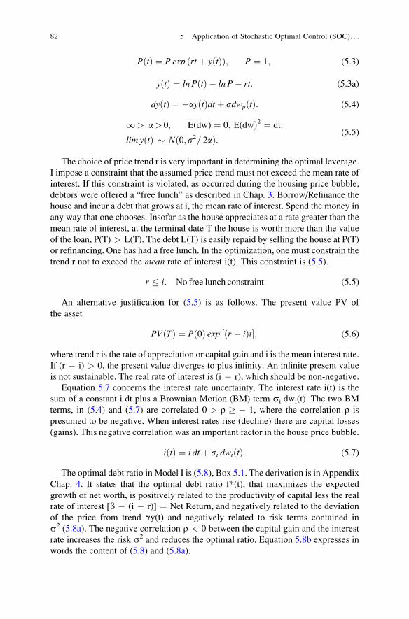
PðtÞ ¼ P exp ðrtþ yðtÞÞ; P ¼ 1; (5.3)

yðtÞ ¼ ln PðtÞ � ln P� rt: (5.3a)

dyðtÞ ¼ �ayðtÞdtþ sdwpðtÞ: (5.4)

1> a> 0; E(dw) ¼ 0; E(dwÞ2 ¼ dt:

lim yðtÞ � Nð0; s2= 2aÞ: (5.5)

The choice of price trend r is very important in determining the optimal leverage.

I impose a constraint that the assumed price trend must not exceed the mean rate of

interest. If this constraint is violated, as occurred during the housing price bubble,

debtors were offered a “free lunch” as described in Chap. 3. Borrow/Refinance the

house and incur a debt that grows at i, the mean rate of interest. Spend the money in

any way that one chooses. Insofar as the house appreciates at a rate greater than the

mean rate of interest, at the terminal date T the house is worth more than the value

of the loan, P(T) > L(T). The debt L(T) is easily repaid by selling the house at P(T)

or refinancing. One has had a free lunch. In the optimization, one must constrain the

trend r not to exceed the mean rate of interest i(t). This constraint is (5.5).

r � i: No free lunch constraint (5.5)

An alternative justification for (5.5) is as follows. The present value PV of

the asset

PVðTÞ ¼ Pð0Þ exp ½ðr � iÞt�; (5.6)

where trend r is the rate of appreciation or capital gain and i is the mean interest rate.

If (r � i) > 0, the present value diverges to plus infinity. An infinite present value

is not sustainable. The real rate of interest is (i � r), which should be non-negative.

Equation 5.7 concerns the interest rate uncertainty. The interest rate i(t) is the

sum of a constant i dt plus a Brownian Motion (BM) term si dwi(t). The two BM

terms, in (5.4) and (5.7) are correlated 0 > r � � 1, where the correlation r is

presumed to be negative. When interest rates rise (decline) there are capital losses

(gains). This negative correlation was an important factor in the house price bubble.

iðtÞ ¼ i dtþ si dwiðtÞ: (5.7)

The optimal debt ratio in Model I is (5.8), Box 5.1. The derivation is in Appendix

Chap. 4. It states that the optimal debt ratio f*(t), that maximizes the expected

growth of net worth, is positively related to the productivity of capital less the real

rate of interest [b � (i � r)] ¼ Net Return, and negatively related to the deviation

of the price from trend ay(t) and negatively related to risk terms contained in

s2 (5.8a). The negative correlation r < 0 between the capital gain and the interest

rate increases the risk s2 and reduces the optimal ratio. Equation 5.8b expresses in

words the content of (5.8) and (5.8a).


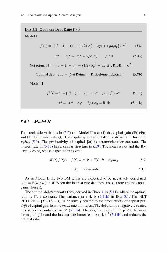
Box 5.1 Optimum Debt Ratio f*(t)

Model I

f �ðtÞ ¼ f½ b� (i� rÞ� � ð1=2Þ s2p � ayðtÞ þrsispg= s2 (5.8)

s2 ¼ sp2 þ sy2 � 2rsisp r< 0 (5.8a)

Net return N ¼ {[b � (i � r)] � (1/2) sp2 � ay(t)}, RISK ¼ s2

Optimal debt ratio ¼ ½Net Return� Risk elements]/Risk, (5.8b)

Model II

f �ðtÞ¼ f � ¼ [ bþ ( p� i)� ðsp2 � rsispÞ�= s2 (5.11)

s2 ¼ si2 þ sp2 � 2rsisp ¼ Risk (5.11b)

5.4.2 Model II

The stochastic variables in (5.2) and Model II are: (1) the capital gain dP(t)/P(t)

and (2) the interest rate i(t). The capital gain has a drift of p dt and a diffusion of

spdwp (5.9). The productivity of capital b(t) is deterministic or constant. The

interest rate in (5.10) has a similar structure to (5.9). The mean is i dt and the BM

term is sidwi whose expectation is zero.

dPðtÞ =PðtÞ þ bðtÞ ¼ p dtþ bðtÞ dtþ spdwp (5.9)

iðtÞ ¼ i dtþ sidwi (5.10)

As in Model I, the two BM terms are expected to be negatively correlated,

r dt ¼ E(wbdwi) < 0. When the interest rate declines (rises), there are the capital

gains (losses).

The optimal debt/net worth f*(t), derived in Chap. 4, is (5.11), where the optimal

ratio is f*, a constant. The variance or risk is (5.11b) in Box 5.1. The NET

RETURN ¼ [p + (b � i)] is positively related to the productivity of capital plus

drift of capital gain less themean rate of interest. The debt ratio is negatively relatedto risk terms contained in s2 (5.11b). The negative correlation r < 0 between

the capital gain and the interest rate increases the risk s2 (5.11b) and reduces the

optimal ratio.

5.4 The Stochastic Optimal Control Analysis 83

5.5 Interpretation of Optimal Debt Ratio

Figure 4.3 describes the optimal debt ratio f*(t) in a manner that is valid for either

model. The optimal debt ratio is on the vertical axis. It is (5.8) for Model I and

(5.11) for Model II. The horizontal axis measures the Net Return. The optimal debt

ratio is a linear function of the Net Return. The risk premium is R in Fig. 4.3.

The optimal debt ratio is positive only if the Net Return exceeds the risk premium.

The SOC analysis in Chap. 4 proved that the expected growth of net worth is

maximal along the “optimal debt ratio line”. This line relates the optimal debt

ratio to the net return. The optimal debt ratio is not a constant, but varies directly

with the net return and risk. If the Net Return is N(1), the optimal debt ratio is f*(1).

As the actual debt ratio f(1) rises above the optimal debt ratio the line, the expected

growth declines and the risk rises. If the actual debt ratio is f(1) and the net return is

N(1), there is an excess debt C(t) ¼ f(1) � f*(1) > 0 and the expected growth is

less than maximal. The larger is the excess debt, the lower the expected growth,

the greater is the variance and hence the greater the probability that net worth

will be driven towards zero. An early warning signal of a crisis is an excess debt.

The main conclusion is that it is not the debt per se that leads to a crisis, but it is theexcess debt.

5.6 Empirical Measures of an Upper Bound

of the Optimal and Actual Debt Ratio

The optimum debt ratio f* is based upon the equations in Box 5.1, with the

constraint that the mean real interest rate (i � r) is non negative – to avoid the

“free lunch” difficulty. There are other sensible stochastic processes, discussed in

Chap. 4. No one knows what is the correct way to model the stochastic processes.

My strategy is to derive an upper bound for the optimal debt ratio f*(t) in Box 5.1

which will also be compatible with alternative sensible stochastic processes. Call

the upper bound ratio f**. Then the excess debtC(t) ¼ f(t) � f**(t) is measured as

the actual debt ratio less an upper bound f** ratio. The most problematic issue is

how to measure the stochastic price, the capital gain dP(t)/P(t).

From the histogram of the capital gains in Fig. 2.1, the mean capital gain over the

period 1980q1–2007q4 was 5.4% per annum with a standard deviation of 2.9%.

The 30-year conventional mortgage rate in Fig. 3.3 ranged from 7.4% to 5% pa

from 2002 to 2007. It is reasonable to argue that, over a long period, the appre-

ciation of housing prices was not significantly different from “the mean mortgage

rate of interest”. Define (i � r) as the mean interest rate less the trend growth of

price, called the mean real rate of interest. A value of (i � r) � 0, a non-negative

mean real rate of interest precludes the “free lunch” that characterized the bubble.

Then one component of an upper bound f**(t) in Model I equation (5.8) for the


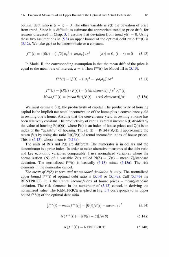
optimal debt ratio is (i � r) ¼ 0. The other variable is y(t) the deviation of price

from trend. Since it is difficult to estimate the appropriate trend or price drift, for

reasons discussed in Chap. 3, I assume that deviation from trend y(t) ¼ 0. Using

these two assumptions in (5.8) an upper bound of the optimal debt ratio f**(t) is

(5.12). We take b(t) to be deterministic or a constant.

f ��ðtÞ ¼ f½bðtÞ � ð1=2Þ sp2 þ rsispg=s2 yðtÞ ¼ 0; ði� rÞ ¼ 0 (5.12)

In Model II, the corresponding assumption is that the mean drift of the price is

equal to the mean rate of interest, p ¼ i. Then f**(t) for Model III is (5.13).

f**(tÞ ¼ ½bðtÞ � ð sp2 � rsispÞ�=s2 (5.13)

f ��ðtÞ ¼ ½ðRðtÞ =PðtÞÞ � ðrisk elementsÞ� = s2>f �ðtÞMean f ��ðtÞ ¼ ½mean RðtÞ=PðtÞ � ðrisk elementsÞ�=s2 (5.13a)

We must estimate b(t), the productivity of capital. The productivity of housing

capital is the implicit net rental income/value of the home plus a convenience yield

in owning one’s home. Assume that the convenience yield in owning a home has

been relatively constant. The productivity of capital is rental income R(t) divided by

the value of housing P(t)Q(t), where P(t) is an index of house prices and Q(t) is an

index of the “quantity” of housing. Thus b (t) ¼ R(t)/P(t)Q(t). I approximate the

return b(t) by using the ratio R(t)/P(t) of rental income/an index of house prices.

This is (5.13), whose mean is (5.13a).

The units of R(t) and P(t) are different. The numerator is in dollars and the

denominator is a price index. In order to make alterative measures of the debt ratio

and key economic variables comparable, I use normalized variables where the

normalization (N) of a variable Z(t) called N(Z) ¼ [Z(t) � mean Z]/standard

deviation. The normalized f**(t) is basically (5.13) minus (5.13a). The risk

elements in the numerator cancel.

The mean of N(Z) is zero and its standard deviation is unity. The normalized

upper bound f**(t) of optimal debt ratio is (5.14) or (5.14a). Call (5.14b) the

RENTPRICE. It is the (rental income/index of house prices � mean)/standard

deviation. The risk elements in the numerator of (5.13) cancel, in deriving the

normalized value. The RENTPRICE graphed in Fig. 5.3 corresponds to an upper

bound f**(t) of the optimal debt ratio.

½ f ��ðtÞ � mean f ��ðtÞ� ¼ ½RðtÞ=PðtÞ � mean:�=s2 (5.14)

Nð f ��ðtÞÞ ¼ ½ðbðtÞ � bÞ�=sðbÞ (5.14a)

Nð f ��ðtÞÞ ¼ RENTPRICE (5.14b)

5.6 Empirical Measures of an Upper Bound of the Optimal and Actual Debt Ratio 85

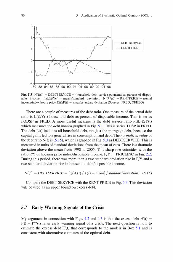
There are a couple of measures of the debt ratio. One measure of the actual debt

ratio is L(t)/Y(t) household debt as percent of disposable income. This is series

FODSP in FRED. A more useful measure is the debt service ratio i(t)L(t)/Y(t)

which measures the debt burden graphed in Fig. 5.1. This is series TDSP in FRED.The debt L(t) includes all household debt, not just the mortgage debt, because the

capital gains led to a general rise in consumption and debt. The normalized value ofthe debt ratio N(f) is (5.15), which is graphed in Fig. 5.3 as DEBTSERVICE. This is

measured in units of standard deviations from the mean of zero. There is a dramatic

deviation above the mean from 1998 to 2005. This sharp rise coincides with the

ratio P/Y of housing price index/disposable income, P/Y ¼ PRICEINC in Fig. 2.2.

During this period, there was more than a two standard deviation rise in P/Y and a

two standard deviation rise in household debt/disposable income.

Nð f Þ ¼ DEBTSERVICE ¼ ½iðtÞLðtÞ = YðtÞ � mean� = standard deviation: (5.15)

Compare the DEBT SERVICE with the RENT PRICE in Fig. 5.3. This deviation

will be used as an upper bound on excess debt.

5.7 Early Warning Signals of the Crisis

My argument in connection with Figs. 4.2 and 4.3 is that the excess debt C(t) ¼f(t) � f**(t) is an early warning signal of a crisis. The next question is how to

estimate the excess debt C(t) that corresponds to the models in Box 5.1 and is

consistent with alternative estimates of the optimal debt.

-2

-1

0

1

2

3

80 82 84 86 88 90 92 94 96 98 00 02 04 06

DEBTSERVICE

RENTPRICE

Fig. 5.3 N[f(t)] ¼ DEBTSERVICE ¼ (household debt service payments as percent of dispos-

able income i(t)L(t)/Y(t) � mean)/standard deviation. N[f**(t)] ¼ RENTPRICE ¼ (rental

income/index house price R(t)/P(t) � mean)/standard deviation (Sources: FRED, OFHEO)


I estimate excess debt C(t) ¼ (f(t) � f**(t)) by using the difference between

two normalized variables N(f) � N(f**), in Fig. 5.3. This difference is measured instandard deviations. Debt service is i(t)L(t)/Y(t) household debt service payments

as percent of disposable income, Fig. 5.1 above, (TDSP in Federal Reserve St.

Louis FRED).

CðtÞ ¼ EXCESSDEBT ¼ N½f ðtÞ� � N½ f ��ðtÞ�¼ Normalized fDEBTSERVICE iðtÞLðtÞ = YðtÞ � RENTPRICERðtÞ =PðtÞg:

(5.15a)

Excess Debt graphed in Fig. 5.4 corresponds to the differenceC(t) ¼ f (t) � f**(t)

on the vertical axis in Fig. 4.3, measured in standard deviations. The SOC analysis

in Chap. 4 proved that the probability of a decline in net worth is positively related to

C(t) the excess debt. As the excess debt rises, the expected growth declines and the

risk increases.

Assume that over the entire period 1980–2007 the debt ratio was not excessive.

There was no excess debt before 1999. During the period 2000–2004, the high

capital gains and low interest rates induced rises in housing prices relative to

disposable income and led to rises in the debt service ratio. By 2004–2005 the

ratio of housing price/disposable income was about three standard deviations above

the long-term mean. See PRICEINC in Fig. 2.2, Chap. 2. This drastic rise alarmed

several economists who believed that the housing market was drastically

overvalued. As indicated in Chap. 2, they were in a minority. It certainly had a

negligible effect upon the market for derivatives and the optimism of the “Quants”.

The advantages of using excess debtC(t) in Fig. 5.4 as an Early Warning Signal

compared to just the ratio of housing price/disposable income are that C(t) focuses

upon the fundamental determinants of the optimal debt ratio as well as upon the

-1.5

-1.0

-0.5

0.0

0.5

1.0

1.5

2.0

2.5

80 82 84 86 88 90 92 94 96 98 00 02 04 06

EXCESSDEBT

Fig. 5.4 Early Warning Signal since 2004. C(t) ¼ EXCESS DEBT ¼ N[f(t)] � N[f**(t)] ¼DEBTSERVICE i(t)L(t)/Y(t) � RENTRATIO R(t)/Y(t)

5.7 Early Warning Signals of the Crisis 87

actual ratio. The excess debt reflects the difference between the debt obligations and

the ability to service them. The probability of declines in net worth, the inability

of the mortgagors to service their debts and the financial collapse due to leverage –

a crisis – are directly related to the excess debt.

Based upon Fig. 5.4, early warning signals were given as early as 2003. By 2005,

the excess debt was about two standard deviations above the mean. Excess debt is

not normally distributed, as is obvious from Fig. 5.4. A probability cannot be

assigned in this case. But whatever the distribution, a 2-3 standard deviation from

the mean must be viewed as an Early Warning Signal (EWS). The actual debt was

induced by capital gains in excess of the mean interest rate. The debt could only be

serviced from capital gains. This situation is unsustainable. When the capital gains

fell below the interest rate, the debts could not be serviced. A crisis was inevitable.

The magnitude of the excess debt in Fig. 5.4 is a benchmark to evaluate that the

economy is being carried away in a bubble. Greenspan, the Fed and IMF had no

concept of this and were oblivious to the EWS since 2004.

5.8 The Market Delusion

A crucial variable in determining the “optimal” debt/net worth in Model I for

example is the trend of the housing price. Figure 5.5 describes the house price

appreciation HPI or capital gains variable CAPGAIN ¼ [P(t) � P(t � 1)]/P(t)

denoted by p(t), which is the four-quarter appreciation of US housing prices,

sample 1991q1–2011q1.

-.08

-.04

.00

.04

.08

.12

92 94 96 98 00 02 04 06 08 10

HPI

Fig. 5.5 Capital gain CAPGAIN ¼ [P(t) � P(t � 1)]/P(t). House Price Index, change over

previous four quarters (e.g. 0.08 ¼ 8% pa) (Federal Housing Finance Industry FHFA USA

Indexes. Sample: 1991q1–2011q1)


In Chap. 3 I explained how the Quants/Market estimated the trend of the

capital gain, with disastrous results. They assumed that the recent capital gains

1994–2004 could continue. These values exceeded the mean rate of interest and

seemed to offer a “free lunch”. My analysis above stresses that optimization

should be based upon the assumption that the mean interest rate must exceed

the longer run capital gain. This was violated from 1998 to 2004. Many were

aware of that but believed that one could get out “as soon as the music stopped”.

This was not possible since they all used the same models and had the same data.

All could not get out at the same time.

5.9 The Shadow Banking System: Leverage

and Financial Linkages

The financial crisis was precipitated by the mortgage crisis for several reasons. First,

a whole structure of financial derivatives was based upon the ultimate debtors –

the mortgagors. Insofar as the mortgagors were unable to service their debts, the

values of the derivatives fell. Second, the financial intermediaries whose assets and

liabilities were based upon the value of derivatives were very highly leveraged.

Changes in the values of their net worth were large multiples of changes in asset

values. Third, the financial intermediaries were closely linked – the assets of one

group were liabilities of another. A cascade was precipitated by the mortgage

defaults. Since the “Quants” were following the same rules, the markets would not

be liquid.

Charles Prince (former Citigroup CEO) told the FCIC that: “Securitization could

be seen as a factory line. As more and more of these subprime mortgages were

created as raw material for the securitization process, not surprisingly in hindsight,

more and more of it was of lower and lower quality. At the end of that process, the

raw material going into it was actually of bad quality, it was toxic quality, and that

is what ended up coming out the other end of the pipeline. Wall Street obviously

participated in that flow of activity”.

A summary of the linkages in the financial system, discussed below, is sketched

in Box 5.2. My discussion of the role of the shadow banking system is directly

based upon the FCIC Report. See also the discussion in Chap. 3 on the “Quants”.

The next chapter is devoted to the AIG case. The origination and securitization of

the mortgages relied upon short-term financing from the shadow banking system.

Unlike banks and thrifts with access to deposits, investment banks relied more on

money market funds and other investors for cash. Commercial paper and repo loans

were the main sources. This flood of money and securitization apparently helped

boost home prices from the beginning of 2004 until the peak in April 2005, even

though homeownership was falling.

5.9 The Shadow Banking System: Leverage and Financial Linkages 89

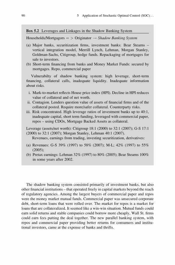
The shadow banking system consisted primarily of investment banks, but also

other financial institutions – that operated freely in capital markets beyond the reach

of regulatory agencies. Among the largest buyers of commercial paper and repos

were the money market mutual funds. Commercial paper was unsecured corporate

debt, short-term loans that were rolled over. The market for repos is a market for

loans that are collateralized. It seemed like a win-win situation. Mutual funds could

earn solid returns and stable companies could borrow more cheaply, Wall St. firms

could earn fees putting the deal together. The new parallel banking system, with

repos and commercial paper providing better returns for consumers and institu-

tional investors, came at the expense of banks and thrifts.

Box 5.2 Leverages and Linkages in the Shadow Banking System

Households/Mortgagors ¼ > Originator ! Shadow Banking System

(a) Major banks, securitization firms, investment banks: Bear Stearns –

vertical integration model, Merrill Lynch, Lehman, Morgan Stanley,

Goldman-Sachs, Citigroup, hedge funds. Repackaging of mortgages for

sale to investors.

(b) Short-term financing from banks and Money Market Funds: secured by

mortgages. Repo, commercial paper

Vulnerabilty of shadow banking system: high leverage, short-term

financing, collateral calls, inadequate liquidity. Inadequate information

about risks.

i. Mark-to-market reflects House price index (HPI). Decline in HPI reduces

value of collateral and of net worth.

ii. Contagion. Lenders question value of assets of financial firms and of the

collateral posted. Require more/safer collateral. Counterparty risks.

iii. Risk concentrated. High leverage ratios of investment banks up to 40:1,

inadequate capital, short term funding, leveraged with commercial paper,

repos – using CDOs, Mortgage Backed Assets as collateral.

Leverage (assets/net worth): Citigroup 18:1 (2000) to 32:1 (2007); G-S 17:1

(2000) to 32:1 (2007); Morgan Stanley, Lehman 40:1 (2007).

Revenues, earnings from trading, investing securitization, derivatives:

(a) Revenues: G-S 39% (1997) to 58% (2007); M-L; 42% (1997) to 55%

(2005);

(b) Pretax earnings: Lehman 32% (1997) to 80% (2005); Bear Stearns 100%

in some years after 2002.


Over time, investment banks and securities firms used securitization to mimic

banking activities outside the regulatory framework. For example, whereas banks

traditionally took money from deposits to make loans and held them to maturity, the

investment banks used money from the capital market, often from Money Market

Mutual Funds, to make loans, package them into securities to sell to investors.

From 2000 to 2007, large banks generally had leverage (assets/net worth) ratios

from 16:1 and then up to 32:1 by the end of 2007. Because investment banks were

not subject to the same capital requirements as commercial and retail banks, they

were given greater latitude to rely on internal risk models in determining capital

requirements, and reported higher leverage. At Goldman-Sachs, leverage increased

from 17:1 (2001) to 32:1 (2007). Morgan Stanley and Lehman reached 40:1 at the

end of 2007. Trading and investments, including securitization and derivative

activities, generated an increasing amount of investment banks’ revenues and

earnings. At G-S, revenues from trading and principal investments increased from

39% (1997) to 58% (2007). At Merrill Lynch revenue from those activities rose

from 42% (1997) to 55% (2005). At Lehman, similar activities generated 80% of

pre-tax earnings in 2005 up from 32% in 1997. At Bear Stearns, they accounted for

100% of pre-tax earnings in some years after 2002.

Foreign investors sought the high-grade securities but at a higher return than

obtained on US Treasuries. They found triple-A assets flowing from the Wall St.

securitization machine. As overseas demand drove up prices of securitized debt,

it created an irresistible profit opportunity for the US financial system to engineer

“quasi-safe” debt instruments by bundling riskier assets and selling senior tranches.

See the discussion in Chap. 3. The US housing bubble was financed by large capital

inflows, as occurred in Ireland and Spain discussed in a later chapter.

Some of the key players in the financial network were Lehman, Citigroup, Bear

Stearns and Merrill Lynch. Since the late 1990s Lehman had built a large mortgage

arm, a formidable securities issuance business and a powerful underwriting as well.

Lehman moved to a more aggressive growth including greater risk and more

leverage. It moved to a “storage” business where Lehman would make and hold

longer-term investments. Across both the commercial and residential sectors, the

mortgage related assets on Lehman’s books increased from $52 billion (2005) to

$111 billion (2007). This would lead to Lehman’s undoing a year later. Lehman’s

regulators were aware of this but did not restrain its activities.

As late as July 2007, Citigroup was still increasing its leveraged loan business.

Citigroup broke new ground in the CDO market. It retained significant exposure to

potential losses on its CDO business, particularly with Citibank – the $1 trillion

commercial bank whose deposits were insured by the FDIC. In 2005 Citigroup

retained the senior and triple-A tranche of most of the CDOs it created. In many

cases, Citigroup obtained protection from a monoline insurer. Because these hedges

were in place, Citigroup presumed that the risk associated with the retained tranches

had been neutralized.

Citigroup reported these tranches at values for which they could not be sold,

raising questions about the accuracy of reported earnings. Part of the reason for

retaining exposures to super-senior positions in CDOs was their favorable capital


treatment. Under the 2001 Recourse Rule, banks were allowed to use their own

models to determine how much capital to hold, an amount that varied according to

how much the market prices moved. Citigroup judged that the capital requirements

for the super-senior tranches of synthetic CDOs it held for trading purposes was

effectively zero, because the prices did not move much. As a result, Citigroup held

little regulatory capital against the super-senior tranche.

Merrill Lynch focused on the CDO business to boost revenue. To keep its CDO

business going, M-L pursued several strategies, all of which involved repackaging

riskier mortgages more attractively or buying its own products, when no one else

would like to do it. Like Citigroup, M-L increasingly retained for its own portfolio

substantial portions of the CDOs it was creating, mainly the super-senior tranches

and it increasingly repackaged the hard to sell BBB rated and other low rated

tranches into other CDOs. Merrill-Lynch continued to push its CDO business

despite signals that the market was weakening.

The bust showed the weaknesses of the system based upon the homeowners’

mortgage debt. Early 2007, it became obvious that home prices were falling in regions

that had once boomed, and that mortgage originators were floundering and that more

and more would be unable to make mortgage payments. The question was how thehousing price collapse would affect the financial system that helped inflate the bubble.In theory – held by Greenspan, Bernanke and the market – securitization, over the

counter derivatives and the shadow banking system was supposed to distribute risk

efficiently among investors. In fact, much of the risk of mortgage backed securities

had been taken by a small group of systemically important companies, with huge

exposures to senior triple-A tranches of CDOs that supposedly were “super-safe”.

As 2007 went on, increasing mortgage delinquencies and defaults compelled the

rating agencies to downgrade the mortgage backed securities and then the CDOs.

Mortgage delinquencies had hovered around 1% during the early part of the decade

jumped in 2005 and kept climbing to 9.7% at the end of 2009. Alarmed investors

sent CDO prices plummeting. Hedge funds faced with margin calls from their repo

lenders were then forced to sell at distressed prices. Many would shut down. Banks

wrote down the value of their holdings by billions of dollars.

By the end of 2008, more than 90% of all tranches of the CDOs had been

downgraded. Moody’s downgraded nearly all of the Baa CDO tranches.

The downgrades were large. More than 80% of Aaa and all of the Baa CDO

bondswere eventually downgraded to junk. As market prices of CDOs dropped,

“Mark-to-Market” (M-t-M) accounting rules require firms to write down their

holdings to reflect the lower market prices. The M-t-M write downs were required

on many securities even if there were no actual realized losses, and in some case,

even if the firms did not intend to sell the securities.

Determining the market value of securities that did not trade was difficult and

subjective and became a contentious issue during the crisis, because the write-

downs reduced earning and triggered collateral calls. Large, systemically important

firms with significant exposure to these securities would be found to be holding very

little capital to protect against potential losses. See Chap. 6 on AIG. Most of these


companies would turn out to be considered by the authorities as “too big to fail” in

the midst of the financial crisis.

When the crises began, uncertainty and leverage would promote contagion.Investors realized that they had limited information about the mortgage assets

that banks and investment banks held and to which they were exposed. Financial

institutions had leveraged themselves with commercial paper, with derivatives and

in the short term repo market, in part using CDOs as collateral. Lenders questioned

the value of assets that these companies had posted as collateral at the same time

that they were questioning the value of those companies’ balance sheets.

Bear Stearns (B-S) hedge funds had significant subprime exposure and were

affected by the collapse of the housing bubble. The collapse produced pressure on

the parent company. The commercial paper and repo markets – the two key

components of the shadow banking lending market – quickly reflected the impact

of the housing bubble collapse, because of the decline of the value of collateral and

concern about the firms’ subprime exposure.

In July 2007, B-S hedge funds failed. Its repo lenders – mostly money market

mutual funds – required that B-S post more collateral and pay higher interest rates.

Mortgage securitization was the biggest piece of B-S most profitable portfolio

division. In mortgage securitization, B-S followed a vertically integrated model

that made money at every step, from loan origination through securitization and

sale. It both acquired and created its own captive organization from originating and

securitization/bundling of mortgages into securities that were then sold to investors.

Nearly all hedge funds provide their investors with market value reports, based

upon computed M-t-M prices for the fund’s various investments. For mortgage

backed investments, M-t-M assets was an extremely important exercise, because

market values (1) were used to inform investors, (2) to calculate the hedge fund’s

total value for internal risk management purposes and (3) because these assets were

held as collateral for repo and other lenders. The crux was that if the value of a

hedge fund’s portfolio declined, repo and other lenders might require more collat-

eral. Many repo lenders sharpened their focus on the valuation of any collateral with

potential subprime exposure. Lenders required increased margins on loans to

institutions that appeared to be exposed to the mortgage market. They often

required Treasury securities as collateral. Triple-A rated mortgage-backed

securities were no longer considered super-safe investments.

Bankers and regulators knew that other investment banks shared B-S

weaknesses: leverage, reliance on overnight funding, concentration in illiquid

mortgages. As Bear Stearns hedge funds were collapsing, the market viewed Bear

Stearns as “the canary in the mine shaft”. During all of this Bernanke was not

unduly unperturbed. In his testimony to the Joint Economic Committee March 28,

2007, he said: “The impact on the broader economy and financial markets of the

problems in the subprime market seems likely to be contained”.

Lehman Brothers was another key player and here is where solvency and

liquidity interacted. If assets are greater than liabilities, net worth (capital) is

positive and the firm is solvent. If not, the firm is in danger of bankruptcy.

In August 2008, shareholder equity was $28 billion. However, balance sheet net


worth (capital) is not relevant if the firm is suffering a massive run. If there is a run,

and a firm can only get fire sale prices for assets, even large amounts of capital can

disappear almost overnight. The chief concerns were Lehman’s real estate related

investments and its reliance on short term funding, including $7.8 billion of

commercial paper and repos as of the end of 2008q1. People were demanding

liquidity from Lehman, which it did not have.

The most pressing danger was the potential failure of the repo market. The little

regulated repo market grew from an average daily volume $800 billion (2002) to

$2.8 trillion (2008). It had become a very deep and liquid market. Even though most

borrowers rolled over repos overnight, it was considered a very safe market because

transactions were over collateralized, the ratio of loans/collateral was less than

unity. Even long term repo loans had to be unwound every day. To the surprise of

both lenders and regulators, as a result to the failure of B-S hedge funds, high

quality collateral was not enough to ensure access to the repo market.

If lenders had to sell off large amounts of collateral in order to meet their own

cash needs, that action would lead to widespread fire sales of repo collateral and

runs by lenders. Most of the Over the Counter derivatives dealers hedge their

contracts with offsetting contracts, creating the potential for a series of losses and

defaults. This was a systemic risk to the financial system as a whole.

In March 2008 the Fed provided a loan to facilitate JP Morgan’s purchase of

B-S. Bernanke refused to lend to Lehman, because Lehman did not have sufficient

collateral. This inconsistency has been the subject of intense debate. See Chap. 6 for

the AIG case.

5.9.1 Summary

One may summarize the crisis in the following way. Chairman Greenspan injects

reserves/lowers short-term interest rates in response to the bursting dot-com bubble.

Mortgage rates fall spurring refinances and speculative interest in the housing

market. House prices start rising, reducing current Loan/Values and creating

perception of reduced credit risk in mortgage lending. Banks securitize mortgage

loans into mortgage backed securities MBS which in turn are resecuritized into

CDOs, and are met with astounding investor demand from yield-hungry

institutions. As investor demand drives down securitization costs, banks reduce

mortgage yields and loosen credit standards to entice more borrowers into the

market. These borrowers in turn drive housing demand upward leading to high

rates of House Price Appreciation which in turn lower perceived probabilites of

losses and therefore reduce perceived credit risk and risk premia required by MBS

investors. Banks continue to earn high fees and spreads by originating and then

selling mortgage risk off their balance sheets, rating agencies continue to earn high

fees from rating MBS and CDOs, securities firms earn their bid/offer spreads, and

real estate speculators continue to flip houses and mortgagors live well above their

means enjoying their free lunches. Then, enough people start realizing that the


house price to rental ratio is “too high”, that the house price to median income ratio

is “too high” and as soon as house prices level off (not even start to fall) borrowers

who never could afford the debt service costs are caught in a situation where they

can no longer sell and pay off their loans at a profit or refinance based on the capital

appreciation of the property. Then the cascade downward begins.

My conclusions are consistent with those of Juselius–Kim. “When is financial

stability jeopardized by systemic events? Is there a maximum sustainable debt

burden. . .? If there is, can it be empirically estimated and will exceeding it neces-

sarily result in a crisis? These are timely and important questions in the wake of the

recent financial crisis and its evolution, yet empirical evidence on these issues is

rather scarce. Using data on aggregate US credit losses, we show that debt

sustainability depends on financial obligations ratios (interest payments and

amortizations relative to income) . . .. In particular, we are able to estimate threshold

values, interpreted as maximum sustainable debt burdens, for the financial stability

is jeopardized by systemic events.” I differ from them insofar as it was the excess

debt that led to the crisis, whose severity was aggravated by the leverages in the

financial sector.

References

Bielecki, T.R., and S. Pliska. 1999. Risk sensitive dynamic risk management. Applied MathematicalOptimization 39: 337–350.

Congressional Oversight Panel (COP). 2011. Report on troubled assets relief program, March.

Washington, DC.

Congressional Oversight Panel (COP). 2009. Special report on regulatory reform,Washington, DC.

Demyank, Y., and O. Van Hemert. 2008. Understanding the subprime mortgage crisis, SSRN

working paper.

Federal Housing Finance Agency. House Price Index USA OFHEO House Price Index http://

www.fhfa.gov.

Federal Reserve Bank, St. Louis. FRED data bank.

Financial Crisis Inquiry Report, FCIC. 2011. Public affairs. New York.

Fleming, W.H. 1999. Controlled Markov processes and mathematical finance. In Nonlinearanalysis, differential equations and control, ed. F.H. Clarke and R.J. Stern. Dordrecht: Kluwer.

Juselius, M., and M. Kim 2011. Sustainable financial obligations and crisis cycles, HECER

discussion paper 313.

Office of Federal Housing Price Oversight (OFHEO).

Platen, E., and R. Rebolledo. 1995. Principles for modeling financial markets. Journal of AppliedProbability 33: 501–530.

References 95

Chapter 6

AIG in the Crisis

Abstract The financial structure of the derivatives insured by AIG with credit

default swaps (CDS) was ultimately related to the systemic risk from the inability of

the mortgagors to service their debts. AIG made several serious mistakes. First: The

estimate of the drift of the capital gain, which drove the bubble, was based upon the

unsustainable growth of the housing price index 2004–2006. A collapse would

occur when the unsustainable capital gain declined below the interest rate. Second,

risk was underestimated because AIG ignored the negative correlation between the

capital gains and the liabilities/claims. The CDS claims grew when the value of the

insured obligations declined. This set off collateral requirements, and the stability

of AIG was undermined. The solution for the optimal insurance liabilities on the

basis of SOC is derived. The SOC approach is a generalization of the contributions

of the economics and actuarial literature. The chapter concludes with an evaluation

of the government bailout.

6.1 Introduction

At its peak, American International Group (AIG) was one of the largest and most

successful companies in the world boasting a Triple-A credit rating, over $1 trillion

in assets, and 76 million customers in more than 130 countries. Yet the sophistica-

tion of AIG’s operations was not matched by an equally sophisticated risk-manage-

ment structure. This poor management structure, combined with a lack of

regulatory oversight, led AIG to accumulate staggering amounts of risk, especially

in its subsidiary, AIG Financial Products (AIGFP). I draw upon the Congressional

Oversight Panel Report (COP 2010) that describes AIG’s role in the financial

market crisis.

Section 6.1 describes what happened to AIG in the 2007–2008 crisis. Section 6.2

sketches the economics literature and the actuarial literature. The conclusions from

the economics literature are that “Despite extensive researches about the

determinants of corporate capital structure, the theories of capital structure remain


97

one of the most controversial issues in modern corporate finance” (Shim 2010).

The actuarial literature on capital requirements and risk was discussed in Chap. 4.

The stochastic optimal (SOC) approach in the following sections is a generalization

of the contributions of the economics and actuarial literature. Its components are:

the criterion function, the stochastic differential equations, and the stochastic

processes. The solution for the optimal capital requirement on the basis of SOC is

in Sect. 6.5. Section 6.6 is an evaluation of the government bailout.

6.2 AIG

AIG occupied an important role in the financial system. Of all the possible losers in

the financial crisis discussed in Chap. 5, AIG should have been the most concerned

with risk management. The AIG Financial Products AIGFP subsidiary sold credit

default swaps (CDSs) involving three parties. Party 1 the obligor sells the “refer-

ence securities” to party 2. The latter are security houses, hedge funds that purchase

protection from party 3, who are banks and insurance companies, which issue the

protection. In many cases municipalities are required to carry insurance in order to

market their bonds, or to obtain a high credit rating. The CDS are privately

negotiated contracts that function in a similar manner to insurance contacts, but

their payoff structure is closer to a put option.

AIGFP’s obligations were guaranteed by AIG’s triple-A rating, which facilitated

borrowing at low interest rates. Ultimately, however, it made it difficult to isolate

AIGFP from its parent, with disastrous consequences. Bernanke characterized

AIGFP as a hedge fund attached to a large and stable insurance company. AIGFP

entered the credit derivatives market in 1998 when it underwrote its first CDS.

Over time AIGFP became a central player in the fast-growing CDS market.

AIGFP’s corporate arbitrage CDS portfolio was comprised of CDS contracts

written on corporate debt and collateralized loan obligations (CLOs). The collateral

pools backing the corporate debt portfolio included baskets of investment-grade

corporate bonds and loans of commercial and industrial loans of large banks. The

collateral pools backing the multi-sector CDOs included prime, Alt-A, and

subprime residential mortgage-backed securities (RMBS), commercial mortgage-

backed securities (CMBS), other asset-backed securities (ABS). CDS written on

corporate debt, CLOs, and multi-sector CDOs serve as protection against “credit

events” of the issuer of the reference obligation, including bankruptcy, failure to

pay, acceleration of payments on the issuer’s obligations, default on the issuer’s

obligations, restructuring of the issuer’s debt, and similar events.

AIGFP’s operating income grew from $131 million in 1994 to $949 million in

2006, 18% pa, paralleling the boom in the overall derivatives market, as well as the

CDS market. While the credit markets provided a source of steady profits for

AIGFP, the division’s operating income represented a relatively small percentage

of AIG’s total operating income, contributing just 7% to firm-wide net income in

2006. More importantly, as events made clear, the risk involved in this business was

98 6 AIG in the Crisis

dramatically disproportionate to the revenue produced. For example, losses in 2007totaled $11.5 billion, twice the aggregate net income produced by this division from1994 to 2006.

AIGmodels showed that there would be no defaults on any of the bond payments

that AIG swaps had insured. AIGFP did not have its own model or otherwise try to

value the CDO portfolio that it guaranteed through CDS nor did it hedge its

exposure. AIG mistakenly believed that it would only have to pay counterparties

if holders of the super-senior tranches insured incurred actual losses. AIGFP relied

on Gorton’s actuarial model that did not provide a tool for monitoring the CDO’s

market value. Gorton’s model had determined with 99.85% confidence that the

owners of super-senior tranches of the CDO’s insured by AIGFP would never suffer

real economic losses (FCIC, pp. 266–267). The company’s auditor PWC apparently

was also not aware of the collateral requirements. PWC concluded that “..the risk of

default on the [AIG] portfolio has been effectively removed as a result of a risk

management perspective. . .”.The bankruptcy of Lehman Brothers was a cataclysmic event. Investors began to

compare the types of securities held by AIG and by Lehman. Goldman-Sachs was

an AIG counterparty, which was very much concerned with the value of AIG’s

collateral. The G-S executives concluded that the Gorton/AIG models were irrele-

vant because the contracts required collateral to be posted if market values of the

insured securities declined, irrespective of only long term cash losses. G-S

estimated that the average decline in the market value of the bonds was 15%.

With leverage this would translate into very large declines in equity.

Until the dispute with G-S, AIG relied on Gorton’s model that did not estimate

the market value of the underlying securities. So G-S mark to market caught AIG by

surprise. By August 2007 AIG publicly disclosed, for the first time, the $79 billion

in CDS’s on super-senior CDO tranches. Sixty four billion were backed by

subprime and nineteen billion were written on risky BBB collateral. By January

2008, AIG still did not have a reliable way to determine the market price of the

securities on which it had written credit protection.

AIG valued its Alt-A and subprime mortgage backed securities at 1.7–2 times

the values used by Lehman. During the summer of 2008, AIG faced increasing

demands from their CDS customers for cash security – collateral calls – totaling

tens of billions of dollars. AIG was not able to provide the required additional

collateral. This put AIG’s credit rating under pressure, which in turn led to even

greater collateral calls, creating even greater pressure on AIG’s credit.

In September 2008, AIG suffered a liquidity crisis, because the firm lacked the

liquidity to meet collateral demands from its customers. In only a matter of months

AIG’s worldwide empire had collapsed, brought down by the company’s

underestimation of risk. The AIG liquidity crisis led to the largest government

bailout of a private company in US history, totaling $182 billion. Maurice

Greenberg, the former CEO, characterized the bailout as a nationalization of

AIG, was bewildered by the situation and was at a loss over how the entire situation

got out of control as it did.

6.2 AIG 99

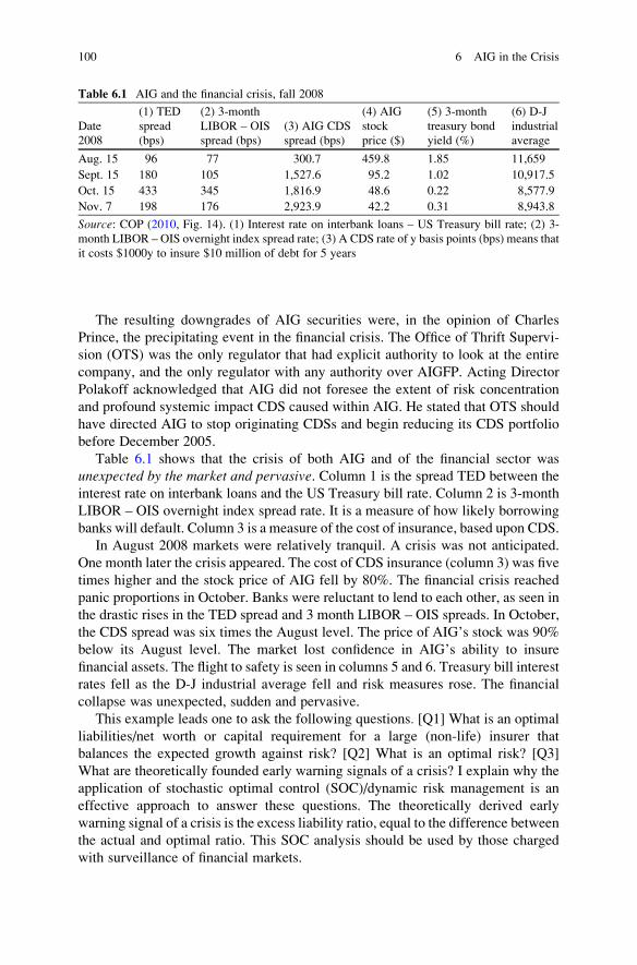
The resulting downgrades of AIG securities were, in the opinion of Charles

Prince, the precipitating event in the financial crisis. The Office of Thrift Supervi-

sion (OTS) was the only regulator that had explicit authority to look at the entire

company, and the only regulator with any authority over AIGFP. Acting Director

Polakoff acknowledged that AIG did not foresee the extent of risk concentration

and profound systemic impact CDS caused within AIG. He stated that OTS should

have directed AIG to stop originating CDSs and begin reducing its CDS portfolio

before December 2005.

Table 6.1 shows that the crisis of both AIG and of the financial sector was

unexpected by the market and pervasive. Column 1 is the spread TED between the

interest rate on interbank loans and the US Treasury bill rate. Column 2 is 3-month

LIBOR – OIS overnight index spread rate. It is a measure of how likely borrowing

banks will default. Column 3 is a measure of the cost of insurance, based upon CDS.

In August 2008 markets were relatively tranquil. A crisis was not anticipated.

One month later the crisis appeared. The cost of CDS insurance (column 3) was five

times higher and the stock price of AIG fell by 80%. The financial crisis reached

panic proportions in October. Banks were reluctant to lend to each other, as seen in

the drastic rises in the TED spread and 3 month LIBOR – OIS spreads. In October,

the CDS spread was six times the August level. The price of AIG’s stock was 90%

below its August level. The market lost confidence in AIG’s ability to insure

financial assets. The flight to safety is seen in columns 5 and 6. Treasury bill interest

rates fell as the D-J industrial average fell and risk measures rose. The financial

collapse was unexpected, sudden and pervasive.

This example leads one to ask the following questions. [Q1] What is an optimal

liabilities/net worth or capital requirement for a large (non-life) insurer that

balances the expected growth against risk? [Q2] What is an optimal risk? [Q3]

What are theoretically founded early warning signals of a crisis? I explain why the

application of stochastic optimal control (SOC)/dynamic risk management is an

effective approach to answer these questions. The theoretically derived early

warning signal of a crisis is the excess liability ratio, equal to the difference between

the actual and optimal ratio. This SOC analysis should be used by those charged

with surveillance of financial markets.

Table 6.1 AIG and the financial crisis, fall 2008

Date

2008

(1) TED

spread

(bps)

(2) 3-month

LIBOR – OIS

spread (bps)

(3) AIG CDS

spread (bps)

(4) AIG

stock

price ($)

(5) 3-month

treasury bond

yield (%)

(6) D-J

industrial

average

Aug. 15 96 77 300.7 459.8 1.85 11,659

Sept. 15 180 105 1,527.6 95.2 1.02 10,917.5

Oct. 15 433 345 1,816.9 48.6 0.22 8,577.9

Nov. 7 198 176 2,923.9 42.2 0.31 8,943.8

Source: COP (2010, Fig. 14). (1) Interest rate on interbank loans – US Treasury bill rate; (2) 3-

month LIBOR – OIS overnight index spread rate; (3) A CDS rate of y basis points (bps) means that

it costs $1000y to insure $10 million of debt for 5 years


6.3 The Economics and Actuarial Literature

Since the Modigliani-Miller irrelevance proposition, and despite extensive research

for decades, there is little consensus on how firms choose their capital structure

(Shim 2010). Both the literature and regulations have departed greatly from the

irrelevance proposition. The banking studies use the ratio of risk weighted assets/

total assets as a measure of portfolio risk (Aggarwal and Jacques 1998). It is based

upon the view that portfolio risk is mostly determined by how assets are allocated

and the different risk types. This is inadequate for an insurance industry, since the

liability side of the portfolio must also be taken into account. Hence an alternative

measure of portfolio risk for an insurer is the volatility of asset/liability ratio

(Cummins and Sommer 1996). This measure takes into account the variance/

covariance matrix between the vectors of assets and liabilities. The appropriate

level of capital is determined mostly by the insurer’s risk exposure.There is a variety of theories. The tradeoff theory postulates that firms seek to

maintain a target/optimal debt ratio by balancing the tax advantages of debt financing

against the costs of financial distress (Meyers 2001). The target ratios may vary from

firm to firm. The pecking order theory of capital structure states that firms prefer

retained earnings as the main source of financing new investment followed by debt

financing followed by new issues of equity. Thusmore profitable firms have less need

for leverage. The financial theory suggests that capital structure is determined by firm

specific characteristics such as profitability, growth opportunities and size of firm.

Korteweg (2010) reviews the literature on net benefits to leverage and then

estimates the market’s valuation of the net benefits to leverage by using panel

data from 1994 to 2004, identified from market values and betas of the company’s

debt and equity. The literature tests the trade off between debt versus equity

financing by running cross sectional regressions of leverage on a set of variables

that proxy for the benefits and costs of leverage. The problem with this regression

approach is that it is not possible to detect whether firms have too much or too little

debt. The implicit assumption is that firms are on average optimally leveraged. This

assumption lacks cogency in light of the analysis especially in Chap. 3. High profits

mechanically lower leverage debt/equity so that cross section regressions show a

negative relation between profitability and leverage, even though optimal debt

ratios are positively related to profitability.The article by Volchan (2007) reflects the state of the art in actuarial risk science.

In Chap. 4, I focused upon Volchan’s excellent discussion of the Cramer-Lundberg

model, and I generalized the Classical gambler’s ruin problems. My conclusions in

Chap. 4 were that the Cramer-Lundberg analysis is inadequate to evaluate the risk/

return in the AIG case. First, the asset side of the equation for the change in surplus

is ignored. The insurance company has assets against the liabilities that bring in

income. Second, the value of the claims against AIG are highly negatively

correlated with the value of the assets. When the market value of the insured assets

decline, AIG must either compensate the insurer for the difference or put up more

collateral. Third, the assets that are insured by AIG are quite closely correlated with

the assets in AIG’s portfolio.

6.3 The Economics and Actuarial Literature 101

6.4 Stochastic Optimal Control (SOC) Approachto Optimal Liabilities of a Large Insurer

The message from the actuarial literature above is that a risk measure should reflect

the economic elements to measure risk, the economic situation, and that the problem

is to find the optimal “required capital”, liabilities/net worth, and risk to maximize

expected surplus. Neither the economics literature nor the Cramer-Lundberg litera-

ture surveyed above answers questions [Q1]–[Q3] whereas the (SOC) approach is

directly concerned with these questions. As described above, the AIGFP followed

policies that were far from optimal, which led to the collapse of AIG. I derive a

warning signal of financial difficulty by focusing upon the difference between the

actual liabilities and the optimal liabilities.SOC is a dynamic optimization, where key variables are stochastic, that I apply

to the AIG case. Technical mathematical details are in the appendix to Chap. 4.My criterion function is the maximization of the expected logarithm of surplus

(net worth) at a future date. Surplus X ¼ A� L is assets A less L liabilities. This

is: V Xð Þ ¼ max InX Tð Þ at terminal date T. There are several advantages of this

criterion. First, it is a risk averse strategy because the logarithm is a concave

function. Unexpected bad events are weighted more heavily than unexpected

good events. Second, the focus is upon the surplus X, which is an objective measure

of economic performance. This measure of performance is relevant for

stockholders, the parties that are insured by the firm and regulators. The control

variable of the insurance company is the ratio of insurance liabilities/surplus. The

ratio of assets/surplus ¼ leverage is equal to one plus the ratio of liabilities/surplus.

The dynamics of the surplus, (6.1) is the sum of several components.

Change in surplus ¼ premium rateð Þ liabilities þ return þ capital gainð Þ assets� claims on the company related to liabilitiesð Þ

ð6:1Þ

The first term in the change in surplus is the premiums, equal to the premium rate

times the insurance liabilities. The second term is the return on assets, which has two

components. The first is the productivity of assets, which is deterministic, and the

second is the capital gain on the assets. The third term concerns claims on the

company that reduce the surplus. Claims may be losses to the insured parties and/or

collateral calls by the parties that have insured assets whose Mark-to-Market (M-t-M)

prices have fallen, as discussed above.

An increase in the liability ratiowill increase expected growth of surplus if the return

on investment plus premiums exceeds the claims. There are two stochastic variables in

this model. First, the productivity of assets is observed, but the future capital gains are

unknownwhen the investment decision ismade.Second, the future claims are unknown

when the insurance policies are sold. Third, there will be a correlation between the

capital gain on assets and the claims. Most certainly, the correlation is negative. When


asset prices, such as the index of housing prices fell, the claims against AIG increased,

either for defaults or for collateral calls. The latter is what led to AIG’s downfall.

The SOC approach derives an optimal liability ratio conditional upon the

stochastic processes. The true stochastic process is unknown. Alternative stochastic

processes imply different optimal liability ratios or optimal leverages. I start with a

general model of the stochastic process and derive the optimal liability/surplus

ratio, optimal risk, and optimal expected growth. Then I consider several

specifications of the stochastic processes, as was done in Chaps. 4 and 5. These

are special cases of the general model. In all cases, the capital gain and claims rate

are negatively correlated. When asset prices fall, insurance claims rise.

A standard of optimality must be based upon sustainable stochastic processes.

By contrast, the market optimized on the basis of unsustainable stochastic pro-

cesses, which led to the bubble and its subsequent collapse.

Given the stochastic process, an optimal liability ratio is derived using the

method explained in Chap. 4, making the appropriate changes. The expected

growth of surplus or net worth is a concave function of the liability ratio,

Fig. 4.2. It is maximal when the optimal ratio is chosen. As the liability ratio

exceeds the derived optimal, the expected growth declines and the risk (variance)

rises, Figs. 4.1 and 4.3. If the liability ratio is less than the optimal, expected growth

is unduly sacrificed to reduce risk. Leverage is equal to one plus the liability ratio;

and the capital requirement is the inverse of the leverage. I focus upon the liability

ratio, and the optimal capital requirement and optimal leverage follow.

The main theoretical results are as follows. (1) The optimal liability ratio is not a

number, but a function. It is proportional to: the drift of the capital gain less the drift

of the claims plus the current productivity of capital plus the insurance premium

rate less a risk premium. The factor of proportionality is the reciprocal of risk

elements. Therefore the optimal liability ratio or capital requirement will vary over

time. (2) Define the excess liability ratio as the actual liability ratio less the optimal

ratio. For a sufficiently high excess liability or debt, the expected growth is zero or

negative and the variance is high. See Figs. 4.1 and 4.2. The probability of a declinein net worth or a debt crisis is directly related to the excess liability or debt ratio.This is our Early Warning Signal (EWS) of a crisis.

6.5 Mathematical Analysis

The expected logarithm of the surplus of the insurer is the growth variable that is

consistent with the insurance literature. Let V X,Tð Þ be the expected logarithm of

surplus X Tð Þ at time T relative to its initial value Xð0Þ. The stochastic optimal

control problem is to select ratios f tð Þ = L tð Þ/X tð Þ of liabilities L tð Þ to surplus X tð Þduring the period 0,Tð Þ that will maximize V X,Tð Þ in (6.2). The maximum value is

V� X,Tð Þ. Ratio f� tð Þ is the optimal leverage, or 1=f� tð Þ is the optimal capital

requirement and will vary over time. The stochastic optimal control tells us what

is an optimal and what is an “excessive” leverage.

6.5 Mathematical Analysis 103

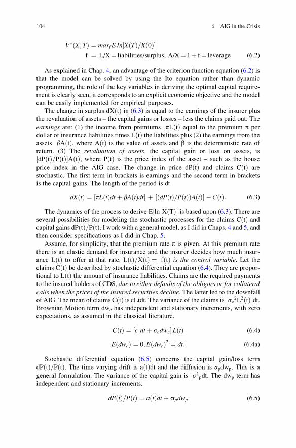
V� X; Tð Þ ¼ maxf E In XðTÞ=Xð0Þ½ �f ¼ L/X¼ liabilities/surplus, A/X¼ 1þ f¼ leverage (6.2)

As explained in Chap. 4, an advantage of the criterion function equation (6.2) is

that the model can be solved by using the Ito equation rather than dynamic

programming, the role of the key variables in deriving the optimal capital require-

ment is clearly seen, it corresponds to an explicit economic objective and the model

can be easily implemented for empirical purposes.

The change in surplus dX tð Þ in (6.3) is equal to the earnings of the insurer plus

the revaluation of assets – the capital gains or losses – less the claims paid out. The

earnings are: (1) the income from premiums pL tð Þ equal to the premium p per

dollar of insurance liabilities times L tð Þ the liabilities plus (2) the earnings from the

assets bA tð Þ, where A tð Þ is the value of assets and b is the deterministic rate of

return. (3) The revaluation of assets, the capital gain or loss on assets, is

dP tð Þ=P tð Þ½ �A tð Þ, where P tð Þ is the price index of the asset – such as the house

price index in the AIG case. The change in price dP tð Þ and claims C tð Þ are

stochastic. The first term in brackets is earnings and the second term in brackets

is the capital gains. The length of the period is dt.

dXðtÞ ¼ pLðtÞdtþ bAðtÞdt½ � þ ðdPðtÞ=PðtÞÞAðtÞ½ � � CðtÞ: (6.3)

The dynamics of the process to derive E ln X Tð Þ½ � is based upon (6.3). There are

several possibilities for modeling the stochastic processes for the claims C tð Þ andcapital gains dP tð Þ=P tð Þ. I work with a general model, as I did in Chaps. 4 and 5, and

then consider specifications as I did in Chap. 5.

Assume, for simplicity, that the premium rate p is given. At this premium rate

there is an elastic demand for insurance and the insurer decides how much insur-

ance L tð Þ to offer at that rate. L tð Þ=X tð Þ ¼ f tð Þ is the control variable. Let theclaims C tð Þ be described by stochastic differential equation (6.4). They are propor-

tional to L tð Þ the amount of insurance liabilities. Claims are the required payments

to the insured holders of CDS, due to either defaults of the obligors or for collateralcalls when the prices of the insured securities decline. The latter led to the downfallof AIG. The mean of claims C tð Þ is cLtdt. The variance of the claims is sc2L2 tð Þ dt.Brownian Motion term dwc has independent and stationary increments, with zero

expectations, as assumed in the classical literature.

CðtÞ ¼ ½c dtþ scdwc� LðtÞ (6.4)

E dwcð Þ ¼ 0;E dwcð Þ2 ¼ dt: (6.4a)

Stochastic differential equation (6.5) concerns the capital gain/loss term

dP tð Þ=P tð Þ. The time varying drift is a tð Þdt and the diffusion is spdwp. This is a

general formulation. The variance of the capital gain is s2pdt. The dwp term has

independent and stationary increments.

dPðtÞ=PðtÞ ¼ aðtÞdtþ spdwp (6.5)


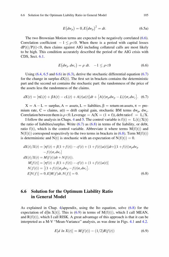
E dwp

� � ¼ 0;E dwp

� �2 ¼ dt: (6.5a)

The two Brownian Motion terms are expected to be negatively correlated (6.6).

Correlation coefficient � 1 � r<0. When there is a period with capital losses

dP tð Þ=P tð Þ<0, then claims against AIG including collateral calls are most likely

to be high. This condition accurately described the period of the AIG crisis with

CDS, Sect. 6.1.

E dwp dwc

� � ¼ r dt: �1 � r<0 (6.6)

Using (6.4, 6.5 and 6.6) in (6.3), derive the stochastic differential equation (6.7)

for the change in surplus dX tð Þ. The first set in brackets contains the deterministic

part and the second set contains the stochastic part: the randomness of the price of

the assets less the randomness of the claims.

dXðtÞ ¼ pLðtÞ þ bAðtÞ � cLðtÞ þ AðtÞaðtÞ½ �dtþ AðtÞspdwp � LðtÞscdwc

� �: (6.7)

X ¼ A� L ¼ surplus, A ¼ assets, L ¼ liabilties, b ¼ return on assets, p ¼ pre-

mium rate, C ¼ claims, a(t) ¼ drift capital gain, stochastic BM terms dwp, dwc.

Correlation between them isr<0. Leverage ¼ A/X ¼ (1 + f)), debt ratio f ¼ L=X.I follow the analysis in Chaps. 4 and 5. The control variable is f tð Þ ¼ L tð Þ=X tð Þ

the ratio of liabilties/surplus. Write (6.7) as (6.8) in terms of the liability, or debt,

ratio f tð Þ, which is the control variable. Abbreviate it where terms M f tð Þð Þ and

N f tð Þð Þ correspond respectively to the two terms in brackets in (6.8). Term M f tð Þð Þis deterministic and N tð Þ is stochastic with an expectation of N f tð Þð Þ ¼ 0.

dXðtÞ=XðtÞ ¼ ½pf ðtÞ þ b 1þ f ðtÞð Þ � cf ðtÞ þ 1þ f ðtÞð ÞaðtÞ dtþ� ½ 1þ f ðtÞð Þspdwp

� f ðtÞscdwc�dXðtÞ=XðtÞ ¼ M f ðtÞð Þdtþ N f ðtÞð Þ:

M f ðtÞ½ � ¼ pf ðtÞ þ b 1þ f ðtÞð Þ � cf ðtÞ þ 1þ f ðtÞð ÞaðtÞ½ �N f ðtÞð Þ ¼ 1þ f ðtÞð Þspdwp � f ðtÞscdwc

� �:

E Nð f Þ½ � ¼ 0;E Mð f Þdt;Nð f Þ½ � ¼ 0: (6.8)

6.6 Solution for the Optimum Liability Ratioin General Model

As explained in Chap. 4/appendix, using the Ito equation, solve (6.8) for the

expectation of d ln X tð Þ½ �. This is (6.9) in terms of M f tð Þð Þ, which I call MEAN,

and R f tð Þð Þ, which I call RISK. A great advantage of this approach is that it can be

interpreted as a M-V “Mean-Variance” analysis, as was done in Figs. 4.1 and 4.2.

E d ln XðtÞ½ � ¼ M f ðtÞð Þ � 1=2ð ÞR f ðtÞð Þ (6.9)

6.6 Solution for the Optimum Liability Ratio in General Model 105

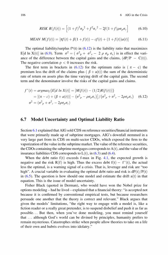
RISK R f ðtÞð Þ ¼ 1þ fð Þ2sp2 þ f 2sc2 � 2f 1þ fð Þrspsch i

(6.10)

MEAN M f ðtÞð Þ ¼ pf ðtÞ þ b 1þ f ðtÞð Þ � cf ðtÞ þ 1þ f ðtÞð ÞaðtÞ½ � (6.11)

The optimal liability/surplus f*(t) in (6.12) is the liability ratio that maximizes

E d ln X tð Þ½ � in (6.9). Term s2 ¼ ð s2p þ s2c � 2 r sp scÞ is in effect the vari-

ance of the difference between the capital gains and the claims, dP=P � C tð Þð Þ.The negative correlation r < 0 increases the risk.

The first term in brackets in (6.12) for the optimum ratio is ð p� cÞ the

premium less the drift of the claims plus bþ a tð Þð Þ the sum of the deterministic

rate of return on assets plus the time varying drift of the capital gain. The second

term and the denominator involve the risks of the capital gains and claims.

f �ðtÞ ¼ argmaxf E d ln XðtÞ½ � ¼ M f ðtÞð Þ � 1=2ð ÞR f ðtÞð Þ½ �f g¼ p� cð Þ þ bþ aðtÞð Þ½ � � s2p � rspsc

� ��= s2p þ s2c � 2rspsc

� �s2 ¼ ðs2p þ s2c � 2rspscÞ

(6.12)

6.7 Model Uncertainty and Optimal Liability Ratio

Section 6.1 explained that AIG sold CDS on reference securities/financial instruments

that were primarily made up of subprime mortgages. AIG’s downfall stemmed in a

very large part from its CDS on multi-sector CDOs, which exposed the firm to the

vaporization of the value in the subprimemarket. The value of the reference securities,

theCDOs containing the subprimemortgages corresponds toA tð Þ, and the value of theinsurance liabilities CDS corresponds to L tð Þ, in (6.3) and (6.4).

When the debt ratio f tð Þ exceeds f-max in Fig. 4.1, the expected growth is

negative and the risk R fð Þ is high. Thus the excess debt f tð Þ � f � tð Þ, the actual

less the optimal, is a warning signal of a crisis. That is, leverage and risk are “too

high”. A crucial variable in evaluating the optimal debt ratio and risk is dP tð Þ=P tð Þin (6.5). The question is how should one model and estimate the drift a tð Þ in that

equation. This is the issue of model uncertainty.

Fisher Black (quoted in Derman), who would have won the Nobel prize for

options modeling – had he lived – explained that a financial theory: “is accepted not

because it is confirmed by conventional empirical tests, but because researchers

persuade one another that the theory is correct and relevant.” Black argues that

given the models’ limitations, “the right way to engage with a model is, like a

fiction reader or a really great pretender, is to suspend disbelief and push it as far as

possible. . . But then, when you’ve done modeling, you must remind yourself

that . . . although God’s world can be divined by principles, humanity prefers to

remain mysterious. Catastrophes strike when people allow theories to take on a life

of their own and hubris evolves into idolatry.”


The question is what is the optimal liability and the excessive liability that should

have been a warning signal for the crisis. How should we model dP tð Þ=P tð Þ ¼a tð Þ dt þ spdwp that corresponds to HPI=CAPGAIN ¼ ½P tþ1ð Þ�P tð Þ�=P tð Þ?Is the capital gain equal to a constant drift aðtÞ¼ a plus a Brownian Motion term,

or is the drift ergodic mean reverting to a constant trend plus a Brownian Motion

term? Are the capital gains terms independent or are they serially correlated? How

can we characterize the distribution of the capital gains?

I approach the problem of deciding on the appropriate way to model the capital

gain equation by looking at Fig. 6.1. It plots the appreciation of single-family

housing prices, CAPGAIN/HPI, a four quarter appreciation of US Housing prices

HPI, percent p.a. It corresponds to dP tð Þ=P tð Þ. Figure 6.1 covers a recent period

1991q1–2011q1, pre and post, crisis. Consider, however, the information available

before the crisis. What can one say about the distribution of the change in house

prices over the period 1980q1–2007q4?

From Figs. 3.4 and 5.2, we can reject the hypothesis that the distribution of the

CAPGAIN series is normal. Table 6.2 tests for serial correlation of the capital gains.

Are they independent? The Q-Statistics reject the null hypothesis that there is no

autocorrelation up to order k. This means that the Brownian Motion assumption

used in modeling dP/P is questionable.

In Chaps. 4 and 5, two models for the capital gain term were considered. In

model I the price P tð Þ was ergodic mean reverting to a constant trend plus a BM

term. In model II, the capital gains term was BM with a constant drift. The choice

between the models depends upon a unit root test. Table 6.3, which tests for a unit

root, is concerned with the question whether or not the capital gains term is

stationary. This is the null hypothesis.

-.08

-.04

.00

.04

.08

.12

92 94 96 98 00 02 04 06 08 10

HPI

Fig. 6.1 HPI/CAPGAIN Capital gains P tð Þ � P t� 1ð Þ½ �=P t� 1ð Þ, percent change in index of

house price HPI, sample 1991q1–2011q1

6.7 Model Uncertainty and Optimal Liability Ratio 107

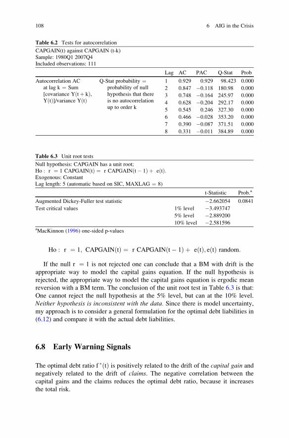
Ho : r ¼ 1; CAPGAIN tð Þ ¼ r CAPGAIN t� 1ð Þ þ e tð Þ; e tð Þ random:

If the null r ¼ 1 is not rejected one can conclude that a BM with drift is the

appropriate way to model the capital gains equation. If the null hypothesis is

rejected, the appropriate way to model the capital gains equation is ergodic mean

reversion with a BM term. The conclusion of the unit root test in Table 6.3 is that:

One cannot reject the null hypothesis at the 5% level, but can at the 10% level.

Neither hypothesis is inconsistent with the data. Since there is model uncertainty,

my approach is to consider a general formulation for the optimal debt liabilities in

(6.12) and compare it with the actual debt liabilities.

6.8 Early Warning Signals

The optimal debt ratio f � tð Þ is positively related to the drift of the capital gain and

negatively related to the drift of claims. The negative correlation between the

capital gains and the claims reduces the optimal debt ratio, because it increases

the total risk.

Table 6.2 Tests for autocorrelation

CAPGAIN(t) against CAPGAIN (t-k)

Sample: 1980Q1 2007Q4

Included observations: 111

Lag AC PAC Q-Stat Prob

Autocorrelation AC

at lag k ¼ Sum

[covariance Y tþ kð Þ,Y tð Þ]/variance Y tð Þ

Q-Stat probability ¼probability of null

hypothesis that there

is no autocorrelation

up to order k

1 0.929 0.929 98.423 0.000

2 0.847 �0.118 180.98 0.000

3 0.748 �0.164 245.97 0.000

4 0.628 �0.204 292.17 0.000

5 0.545 0.246 327.30 0.000

6 0.466 �0.028 353.20 0.000

7 0.390 �0.087 371.51 0.000

8 0.331 �0.011 384.89 0.000

Table 6.3 Unit root tests

Null hypothesis: CAPGAIN has a unit root;

Ho : r ¼ 1 CAPGAIN tð Þ ¼ r CAPGAIN t� 1ð Þ þ e tð Þ:Exogenous: Constant

Lag length: 5 (automatic based on SIC, MAXLAG ¼ 8)

t-Statistic Prob.a

Augmented Dickey-Fuller test statistic �2.662054 0.0841

Test critical values 1% level �3.493747

5% level �2.889200

10% level �2.581596aMacKinnon (1996) one-sided p-values


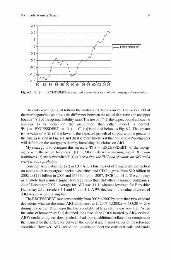
The early warning signal follows the analysis in Chaps. 4 and 5. The excess debt of

themortgagors/households is the difference between the actual debt ratio and an upper

bound f �� tð Þ of the optimal liability ratio. The use of f �� tð Þ the upper, bound allows theanalysis to be done on the assumption that either model is correct.

C tð Þ ¼ EXCESSDEBT ¼ f tð Þ � f �� tð Þ½ � is plotted below as Fig. 6.2. The greater

is the value ofC(t): (a) the lower is the expected growth of surplus and the greater is

the risk, as is seen in Fig. 4.1 and (b) it is more likely is it that households/mortgagors

will default on the mortgages thereby increasing the claims on AIG.

My strategy is to compare this measure C tð Þ ¼ EXCESSDEBT of the mortg-

agors with the actual liabilities L tð Þ of AIG to derive a warning signal. If actualliabilities LðtÞ are risingwhenCðtÞ is increasing, the liklihood of claims onAIG and acrisis is more probable.

Consider AIG liabilities L tð Þ or f tð Þ. AIG’s business of offering credit protectionon assets such as mortgage backed securities and CDO’s grew from $20 billion in

2002 to $211 billion in 2005 and $533 billion in 2007. (FCIC, p. 141). The company

as a whole had a much higher leverage ratio than did other insurance companies.

As of December 2007, leverage for AIG was 11:1, whereas leverage for Berkshire

Hathaway 2:1, Travelers 4:1 and Chubb 4:1. A 9% decline in the value of assets of

AIG would wipe out surplus.

TheEXCESSDEBTrose considerably from2002 to 2007bymore than two standard

deviations, whereas the actual AIG liabilities rose, L(2007)/L(2002) ¼ 533/20 ¼ 26.6

during this period. This means that the probability of large claimswas very high.When

the value of house prices P tð Þ declined, the value of theCDOs insured byAIG declined.

AIG’s credit rating was downgraded, it had to post additional collateral or compensate

the insured for the difference between the notional and market values of the reference

securities. However, AIG lacked the liquidity to meet the collateral calls and banks

-1.5

-1.0

-0.5

0.0

0.5

1.0

1.5

2.0

2.5

80 82 84 86 88 90 92 94 96 98 00 02 04 06

EXCESSDEBT

Fig. 6.2 C tð Þ ¼ EXCESSDEBT, normalized excess debt ratio of the mortgagors/households

6.8 Early Warning Signals 109

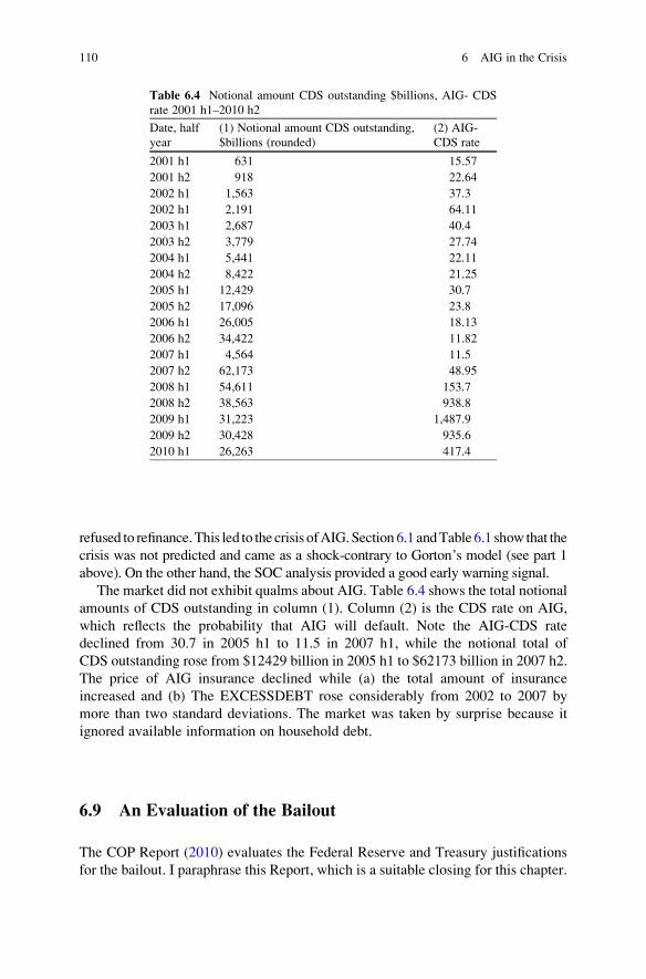
refused to refinance.This led to the crisis ofAIG.Section 6.1 andTable 6.1 show that the

crisis was not predicted and came as a shock-contrary to Gorton’s model (see part 1

above). On the other hand, the SOC analysis provided a good early warning signal.

The market did not exhibit qualms about AIG. Table 6.4 shows the total notional

amounts of CDS outstanding in column (1). Column (2) is the CDS rate on AIG,

which reflects the probability that AIG will default. Note the AIG-CDS rate

declined from 30.7 in 2005 h1 to 11.5 in 2007 h1, while the notional total of

CDS outstanding rose from $12429 billion in 2005 h1 to $62173 billion in 2007 h2.

The price of AIG insurance declined while (a) the total amount of insurance

increased and (b) The EXCESSDEBT rose considerably from 2002 to 2007 by

more than two standard deviations. The market was taken by surprise because it

ignored available information on household debt.

6.9 An Evaluation of the Bailout

The COP Report (2010) evaluates the Federal Reserve and Treasury justifications

for the bailout. I paraphrase this Report, which is a suitable closing for this chapter.

Table 6.4 Notional amount CDS outstanding $billions, AIG- CDS

rate 2001 h1–2010 h2

Date, half

year

(1) Notional amount CDS outstanding,

$billions (rounded)

(2) AIG-

CDS rate

2001 h1 631 15.57

2001 h2 918 22.64

2002 h1 1,563 37.3

2002 h1 2,191 64.11

2003 h1 2,687 40.4

2003 h2 3,779 27.74

2004 h1 5,441 22.11

2004 h2 8,422 21.25

2005 h1 12,429 30.7

2005 h2 17,096 23.8

2006 h1 26,005 18.13

2006 h2 34,422 11.82

2007 h1 4,564 11.5

2007 h2 62,173 48.95

2008 h1 54,611 153.7

2008 h2 38,563 938.8

2009 h1 31,223 1,487.9

2009 h2 30,428 935.6

2010 h1 26,263 417.4


6.9.1 Government’s Justification for Rescue

The Federal Reserve was the only governmental entity at the time with the legal

authority to provide liquidity to the financial system in emergency circumstances.

The Board and FRBNY ultimately chose to provide AIG with assistance after

identifying the systemic risks associated with the company and contemplating the

consequences of an AIG bankruptcy or partial rescue. On September 16, the Board,

with the full support of Treasury, authorized Federal Reserve Bank of New York

(FRBNY) to lend up to $85 billion to AIG in order to assist the company in meeting

its obligations as they came due. The Board determined that, in the then-existing

environment, “a disorderly failure of AIG could add to already significant levels of

financial market fragility and lead to substantially higher borrowing costs, reduced

household wealth, and materially weaker economic performance.”

The Federal Reserve’s actions were based upon its judgment that an AIG collapse

would have been much more severe than that of Lehman Brothers because of its

global operations, substantial and varied retail and institutional customer base, and

the various types of financial services it provided. At September 2008 the time of the

initial decision to assist AIG, the Federal Reserve and Treasury publicly identified

three primary ways in which an AIG failure posed systemic risk. First, they

concluded that, given AIG’s role as a large seller of CDSs on CDOs, an AIG failure

could have exposed its counterparties to large losses and disrupted the operation of

the payments and settlements system. According to Secretary Geithner, if the AIG

parent holding company had filed for bankruptcy, defaults on over $100 billion of

debt and on trillions of dollars of derivatives would have resulted. The Federal

Reserve and Treasury argued that this would have adversely impacted numerous

financial institutions and the financial system as a whole. The primary fear of the

Federal Reserve and Treasury was that defaults directly related to AIG would have

spread throughout the financial system, affecting transactions between other

counterparties, negatively affecting investor confidence, and further destabilizing

the economy. Second, the Federal Reserve and Treasury concluded that an AIG

default on its commercial paper could have adversely impacted money market

mutual funds since AIG had issued $20 billion in commercial paper to money

market mutual funds, approximately four times as much as Lehman Brothers. In

the government’s view, this could have substantially disrupted the commercial paper

market by reducing credit availability for borrowers even on a short-term basis and

causing higher lending rates. This concern escalated after the money market

disruptions that occurred in the wake of the Lehman Brothers bankruptcy filing,

including the “breaking of the buck” at the Reserve Primary Fund.

Third, the Federal Reserve and Treasury asserted that they feared that an AIG

failure could have undermined an already fragile economy byweakening business and

investor confidence. After the placement of Fannie Mae and Freddie Mac into

government conservatorship on September 7 and the Lehman Brothers bankruptcy

filing on September 15, financial markets destabilized considerably. AIG maintained

financial relationships with a large number of banks, insurance companies, and other

6.9 An Evaluation of the Bailout 111

market participants across the globe. A failure of AIG in this environment, according

to the Federal Reserve and Treasury, could have further shaken investor confidence

and contributed to increased borrowing costs and additional economic deterioration.

In this context, the Federal Reserve and Treasury officials stated that they

believed that the unfolding crisis and the increasingly fragile state of the economy

necessitated swift action to prevent a total collapse of the financial system.

6.9.2 Panel’s Analysis of Options Availableto the Government and Decisions

The Panel recognized that policymakers faced a deepening financial crisis and that

there were many issues of serious concern and a limited amount of time in which to

respond to AIG in September 2008. The Panel stated that FRBNY’s decisions were

made in the belief that it alone could act and that it had to choose between options

that were all unattractive. There is nothing unusual about central banks acting as the

lender of last resort. However, by adopting the terms developed by the private

sector consortium and retaining most of its terms and conditions, FRBNY chose to

act in effect as if it were a private investor in many ways, when its actions also had

serious public consequences whose full extent it may not have appreciated. FRBNY

also failed to recognize the AIG problem and get involved at a time when it could

have had more options.

While the reasons for FRBNY’s failure are not clear, it is clear that when

FRBNY finally realized AIG was failing and that there would be no private sector

solution, Chairman Bernanke and President Geithner failed to consider any optionsother than a full rescue. To have the government step in with a full rescue was notthe approach used in prior crises, including Bear Stearns and Long-Term CapitalManagement. FRBNY chose lawyers from a limited pool and did not seek legal

advice from a debtor’s counsel (such as AIG’s bankruptcy counsel or independent

bankruptcy counsel). As a result, there were many options FRBNY evidently did

not consider, including a combined private/public rescue (which would have

maintained some market discipline), a loan conditioned on counterparties granting

concessions, and a short-term bridge loan from FRBNY to provide AIG time for

longer-term restructuring. Providing a full government rescue with no sharedsacrifice among the creditors who dealt with AIG fundamentally changed therelationship between the government and the markets, reinforcing moral hazardand undermining the basic tenets of capitalism. The rescue of AIG dramatically

added to the public’s sense of a double standard – where some businesses and their

creditors suffer the consequences of failure and other, larger, better connected

businesses do not. The FRBNY’s decision-making also suggest that it neglected

to give sufficient attention to the crucial need – more important in a time of crisis

than ever – for accountability and transparency.


The Panel asked: Was It Truly an All-or-Nothing Choice? The Treasury/Fed

presented the decision to rescue AIG as an all-or-nothing “binary” decision.

In other words, the government asserted that it was necessary to rescue AIG in its

entirety or let it fail in its entirety. It was not possible to pick and choose which

businesses or subsidiaries could be saved. The Panel tested this assertion and

considered whether bankruptcy had to be an all-or-nothing option, in terms of the

entities covered, the obligations covered, or in terms of timing. If a bankruptcy was

not a real option in September 2008, was it later?

The potential impact of an AIG bankruptcy can be guessed by examining how

the markets continued to deteriorate even after AIG was rescued. As shown in

Table 6.1, the spread between the London Interbank Offered Rate (LIBOR) and

the Overnight Index Spread Rate (OIS) – used as a proxy for fears of bank

bankruptcy – dramatically increased in September 2008 amid the growing

concerns of financial collapse. Former Federal Reserve Chairman Alan

Greenspan stated that the “LIBOR-OIS spread remains a barometer of fears of

bank insolvency.” In the immediate aftermath of the Lehman bankruptcy this

spread spiked to a level indicating actual illiquidity in the interbank market – not

merely a high cost for obtaining funds – meaning that banks were not willing to

lend to one another. Prior to the beginning of the credit market crisis in August

2007, the LIBOR-OIS spread was 10 basis points. The LIBOR-OIS spread

reflected the contraction of liquidity that crippled the financial markets in 2008,

as seen in Table 6.1.

The Panel recognized that the government was faced with a deepening financial

crisis, and its attention was on a number of troubled institutions besides AIG in the

course of just a few days. Given this context, the government took actions that it

thought would facilitate rapid intervention in the midst of deteriorating economic

conditions. Nonetheless, if the government concluded that it could not impose

conditions on its assistance once it had decided to backstop AIG with taxpayer

funds, or that other possible rescue alternatives were unattractive or impracticable,

then it had an obligation to fully explain why it decided what it did, and especially

why it was of the opinion that all AIG’s creditors and counterparties would receiveall amounts they were owed. In addition, while the Panel acknowledged the number

of complex issues and troubled institutions that policymakers were concerned with

at the time, it appears that the government was neither focused on nor prepared to

deal with the AIG situation. By placing a tremendous amount of faith in the

assumption that a private sector solution would succeed in resolving AIG, the

government had no legitimate alternative on the table once that assumption turned

out to be incorrect. In its assessment of government actions to deal with the current

financial crisis, the Panel has regularly called for transparency, accountability, and

clarity of goals. These obligations on the part of the government do not vanish in the

midst of a financial crisis. In fact, it is during times of crisis, when difficult decisions

must be made, that a full accounting of the government’s actions is especially

important.

6.9 An Evaluation of the Bailout 113

6.10 Conclusions: Lessons to be Learned

From 1994 to 2006 AIGFP operating income grew by 18% pa paralleling the boom

in the overall derivative market as well as in the CDS market. The risk involved in

this business was dramatically disproportionate to the revenue produced. Losses in

one year 2007 totaling $11.5 billion were twice the aggregate net income produced

by the division over the entire period 1994–2006.

AIGFP relied on Gorton’s actuarial model that did not provide a tool for

monitoring the CDO’s market value. Gorton’s model had determined with

99.85% confidence that the owners of super-senior tranches of the CDO’s insured

by AIGFP would never suffer real economic losses. The company’s auditor PWC

apparently was also not aware of the collateral requirements. PWC concluded that

“..the risk of default on the [AIG] portfolio has been effectively removed as a result

of a risk management perspective. . .”. AIG was led to accumulate staggering

amounts of risk, especially in its Financial Products subsidiary.

What lessons can be learned from AIGs experience? AIG made several serious

mistakes. First, the financial structure of derivatives CDS insured by AIG, was

ultimately based upon the systemic risk from the inability of the mortgagors to

service their debts. The exaggerated view of the drift of the capital gain, which drove

the bubble, was based upon the growth of the value of housing, the housing price

index 2004–2006. This growth ranging from 10% to 14% pa exceeded the mean

interest rate. Mortgagors consumed the difference between the refinancing of the

loan and the associated debt. They expected to service their debts from the appreci-

ation of the housing price in excess of the rate of interest. This free lunch woulddisappear when the unsustainable capital gain declined below the interest rate.

Second, risk was underestimated because AIG ignored the negative correlation

between the capital gain and the claims. The CDS claims grew when the value of

the insured obligations CDO declined. This set off collateral requirements and the

stability of AIG was undermined.

Acting Director of the OTS Polakoff acknowledged that AIG and OTS did not

foresee the extent of risk concentration and profound systemic impact CDS caused

within AIG. The AIG crisis leads one to ask the following questions. What is an

optimal liability ratio or capital requirement for a large insurer of financial

derivatives that balances the expected growth against risk? What is an optimal

risk? What are theoretically founded early warning signals of a crisis? Neither the

economics literature nor the Cramer-Lundberg literature answers these questions.

I explained why the application of stochastic optimal control (SOC)/dynamic risk

management is an effective approach to answer these questions. The theoretically

derived early warning signal of a crisis is the excess liability ratio, equal to the

difference between the actual and optimal ratio. This SOC analysis should have

been used by those charged with surveillance of financial markets.


References

Aggarwal, R., and K.T. Jacques. 1998. Assessing the impact of prompt action on bank capital andrisk. New York: Federal Reserve Bank of New York, Economic Policy Review.

Congressional Oversight Panel. 2010. The AIG rescue, its impact on markets and the government’sexit strategy. Washington, DC: U.S.G.P.O.

Cummins, J.D., and D.W. Sommer. 1996. Capital and risk in property–liability insurance markets.

Journal of Banking and Finance 20: 1069–1092.Derman, Emanuel. 2004. My life as a quant. Hoboken: Wiley.

Financial Crisis Inquiry Report, FCIC Final Report of National Commission. 2011. Public Affairs,

New York.

Korteweg, Arthur. 2010. The net benefits to leverage. Journal of Finance LXV(6): 2089–2136.MacKinnon. 1996. Journal of Applied Econometrics.Meyers, S.C. 2001. Capital structure. Journal of Economic Perspectives 15: 81–102.Meyers, S.C., and J.A. Read. 2001. Capital allocation for insurance companies. Journal of Risk

and Insurance 68: 545–580.Shim, Jeungbo. 2010. Capital-based regulation, portfolio risk and capital determinants: Empirical

evidence from US property insurers. Journal of Banking and Finance 34: 250–261.Stein, Jerome L. 2010. Greenspan’s retrospective of financial crisis and stochastic optimal control.

European Financial Management 16: 5858–5871.Volchan, S. 2007. The fundamental theorem of actuarial risk science. The Mathematical Scientist

31(2): 73–84.

References 115

Chapter 7

Crisis of the 1980s

Abstract There have been three crises since the 1930s: the Agricultural crisis

of the 1980s, the S&L crisis in the 1980s and the major financial crisis of 2008.

The two crises of the 1980s had many features in common, but were localized.

The crisis of 2008 shared the common elements of the earlier two but was more

pervasive and severe due to the financial structure that was based upon the housing/

mortgage sector. I focus upon the agriculture crisis. How should creditors, banks

and bank regulators evaluate and monitor risk of an excessive debt that significantly

increases the probability of default? I show how the techniques of stochastic

optimal control used in earlier chapters provided early warning signals of the crisis.

I compare the S&L crisis to the agricultural crisis.

7.1 Introduction

There were three crises since the 1930s: the Agricultural crisis of the 1980s, the

S&L crisis in the 1980s and the major financial crisis of 2008. The two crises of the

1980s had many features in common, but were localized. The crisis of 2008 shared

the common elements of the earlier two but was more pervasive and severe due to

the financial structure that was based upon the housing/mortgage sector. In the

current chapter I focus upon the crises of the 1980s, in particular the agriculture

crisis. This chapter addresses the question: How should creditors, banks and bankregulators evaluate and monitor risk of an excessive debt that significantlyincreases the probability of default? I show how the techniques of stochastic

optimal control used in earlier chapters are useful in providing early warning

signals. In the concluding part I compare the S&L crisis to the agricultural crisis.

The agricultural debt crisis of the 1980s is emblematic of the bubble-crisis

phenomenon. Figure 7.1 graphs the ratio of debt/equity DEBTEQUITY and the

delinquency rate on loans DELIQRATEFCS. The variables have been normalized

to facilitate comparison. N(Z) is (Z-mean)/standard deviation. The agricultural debt

crisis is the shaded area in Fig. 7.1.


117

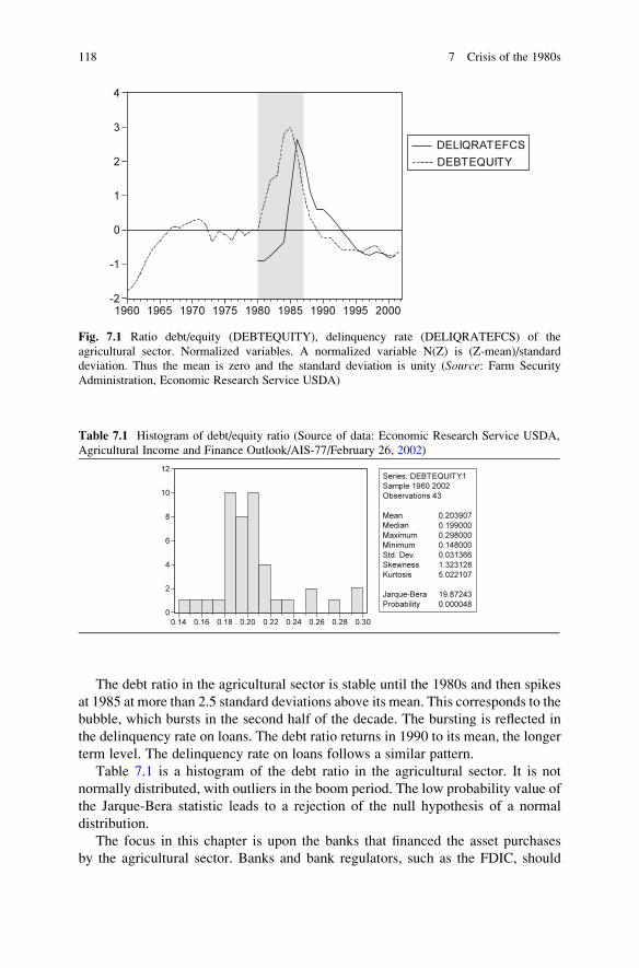
The debt ratio in the agricultural sector is stable until the 1980s and then spikes

at 1985 at more than 2.5 standard deviations above its mean. This corresponds to the

bubble, which bursts in the second half of the decade. The bursting is reflected in

the delinquency rate on loans. The debt ratio returns in 1990 to its mean, the longer

term level. The delinquency rate on loans follows a similar pattern.

Table 7.1 is a histogram of the debt ratio in the agricultural sector. It is not

normally distributed, with outliers in the boom period. The low probability value of

the Jarque-Bera statistic leads to a rejection of the null hypothesis of a normal

distribution.

The focus in this chapter is upon the banks that financed the asset purchases

by the agricultural sector. Banks and bank regulators, such as the FDIC, should

Table 7.1 Histogram of debt/equity ratio (Source of data: Economic Research Service USDA,

Agricultural Income and Finance Outlook/AIS-77/February 26, 2002)

Fig. 7.1 Ratio debt/equity (DEBTEQUITY), delinquency rate (DELIQRATEFCS) of the

agricultural sector. Normalized variables. A normalized variable N(Z) is (Z-mean)/standard

deviation. Thus the mean is zero and the standard deviation is unity (Source: Farm Security

Administration, Economic Research Service USDA)

118 7 Crisis of the 1980s

evaluate whether the borrowers are likely to default. When is the debt ratio“excessive” so that delinquency is likely? What were theoretically based,

objectively measured, early warning signals that should have signaled the agricul-

tural crisis and delinquencies? I apply the same techniques of SOC used in the

previous chapters, to derive the optimal debt in the agricultural sector where there

are risks on both the asset and liability sides of the balance sheet. The ratio of debt/

net worth per se is not a significant explanation of defaults. The vulnerability of the

system to shocks, from either the return to capital, the interest rate or capital gain,

increases directly with the excess debt, which is defined as the actual less the

optimal debt ratio. As the excess debt rises, risk rises relative to expected return

and default becomes more likely. In this manner the SOC approach developed here

should be useful to the FDIC and other bank regulators.

I draw upon the study by the FDIC (1997) to discuss the history of the period:

the cause and development of the bubble and the reason for its collapse.1 Agri-

culture flourished in the 1980s. Farm exports grew rapidly and along with the

domestic inflation farm incomes reached all-time highs. These factors produced

capital gains on farm assets. Equity rose significantly. Credit was readily available.

Real interest rates were low and farmers used the rising value of farm assets as

collateral for loans. Farmers would purchase farm real estate with moderate down

payments and, after the value of the newly purchased land increased, would use the

increased equity to buy additional farmland with minimal down payments. Higher

levels of real estate debt were supplemented by debt to finance machinery and

equipment.

The sequence is described by Fig. 7.2. The speculation in land produced capital

gains and raised the market value of equity (EQUITY). Consequently, the ratio of

interest service on the debt/value added (INTVA), the debt burden, rose significantly.

In the fall of 1979, the Federal Reserve undertook a restrictive monetary policy in

order to reduce inflation, and interest rates rose drastically. The resulting appreciation

of the US dollar reduced foreign demand for US agricultural products. The decline in

foreign demand was exacerbated by the debt crisis in the less developed countries.

Farm exports declined by 40% from 1971 to 1976, at a timewhen productive capacity

had increased. The result was an accumulation of huge surpluses of farm

commodities in the early 1980s. When the bubble collapsed in 1985, asset values

and equity fell drastically. The resulting rise in the debt burden was devastating, and

the (DELINQRATEFCS) delinquency rate on loans rose drastically.

Table 7.2 presents Granger causality tests. Did the return on assets, the sum of

the capital gain and the productivity of capital, “cause” the debt ratio to rise?

Did the rise in the debt ratio “cause” higher capital gains and raise the return?

It seems that at best the rise in the return – capital gain – Granger caused a rise in the

debt/equity ratio. This result is consistent with the story described above and

graphed in Fig. 7.2.

1 See Barry and Robison (2001) and Moss et al. (2003) for a discussion of the agriculture

economics literature.

7.1 Introduction 119

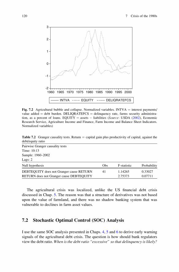
The agricultural crisis was localized, unlike the US financial debt crisis

discussed in Chap. 5. The reason was that a structure of derivatives was not based

upon the value of farmland, and there was no shadow banking system that was

vulnerable to declines in farm asset values.

7.2 Stochastic Optimal Control (SOC) Analysis

I use the same SOC analysis presented in Chaps. 4, 5 and 6 to derive early warning

signals of the agricultural debt crisis. The question is how should bank regulators

view the debt ratio.When is the debt ratio “excessive” so that delinquency is likely?

Table 7.2 Granger causality tests. Return ¼ capital gain plus productivity of capital, against the

debt/equity ratio

Pairwise Granger causality tests

Time: 10:13

Sample: 1960–2002

Lags: 2

Null hypothesis Obs F-statistic Probability

DEBTEQUITY does not Granger cause RETURN 41 1.14265 0.33027

RETURN does not Granger cause DEBTEQUITY 2.75373 0.07711

-2

-1

0

1

2

3

1960 1965 1970 1975 1980 1985 1990 1995 2000

INTVA EQUITY DELIQRATEFCS

Fig. 7.2 Agricultural bubble and collapse. Normalized variables. INTVA ¼ interest payments/

value added ¼ debt burden. DELIQRATEFCS ¼ delinquency rate, farms security administra-

tion, as a percent of loans. EQUITY ¼ assets � liabilities (Source: USDA (2002), Economic

Research Service, Agriculture Income and Finance, Farm Income and Balance Sheet Indicators.

Normalized variables)


The components of the analysis are the criterion function and the stochastic

differential equations.

7.2.1 The Criterion Function

The lender or bank regulator should evaluate what debt ratio maximizes the

expected (E) growth rate of the borrower’s net worth over the period of the loan,

an horizon of length T from the present t ¼ 0. This would be the optimal debt that a

prudent lender would want to offer. The bank/lender wants to avoid borrower’s

bankruptcy (X ¼ 0) by placing a very high penalty on a debt that would lead to a

zero net worth, bankruptcy. The lender is very risk averse.

The borrower has a net worth X(t) equal to the value of assets (used inter-

changeably for capital) K(t) less debt L(t). Initially net worth X ¼ X(0) > 0. Equa-

tion 7.1 is the criterion function. The maximization is over the debt ratios f ¼ L/X.

WðX; TÞ ¼ maxf E ln½XðTÞ=Xð0Þ�; X ¼ K � L> 0; f ¼ L=X: (7.1)

The next steps are to: explain the stochastic differential equation for net worth,

relate it to the debt ratio, and specify what are the sources and characteristics of the

risk and uncertainty.

7.3 Dynamics of Net Worth

In view of (7.1), the bank/lender should focus upon the change in net worth dX(t) of

the borrower. It is the equal to the change in capital dK(t) less the change in debt

dL(t). Capital K ¼ PQ, the product a physical quantity Q times the relative price P

of the capital asset to the price of output. The change in the value of capital has two

components. The first is the change due to the change in relative price of capital,

which is the capital gain or loss, K(dP/P) term. The second is investment, which is

I ¼ P dQ, the change in the quantity times the relative price. The change in debt

dL is the sum of expenditures less income. Expenditures are the debt service r(t)L(t)

at real interest rate r(t), plus investment I ¼ P dQ plus either consumption, dividends

or distributed profits C(t). Income Y(t) ¼ b(t)K(t) is the product of capital times b(t)its productivity. Variable b(t) is defined in (7.2.1) as dP(t)/P(t) + b(t).

For simplicity, assume that consumption C(t) is a constant fraction c > 0 of net

worth X(t), C(t) ¼ cX(t). Combining these effects, the change in net worth is (7.2).

Change in net worth ¼ value of assets (capital gain + productivity of capital) �(interest payments � consumption). Assets ¼ K(t) P(t)Q(t). Interest payments

r(t)L(t), debt L(t), r(t) interest rate.

dXðtÞ ¼ KðtÞ½ dPðtÞ=PðtÞð Þ þ bðtÞ� � rðtÞLðtÞdt� CðtÞdt (7.2)

7.3 Dynamics of Net Worth 121

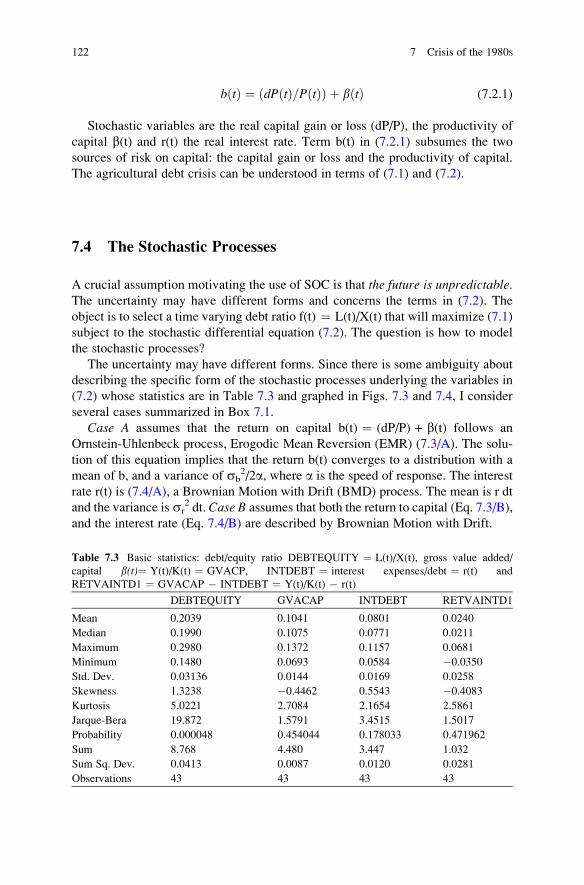
bðtÞ ¼ ðdPðtÞ=PðtÞÞ þ bðtÞ (7.2.1)

Stochastic variables are the real capital gain or loss (dP/P), the productivity of

capital b(t) and r(t) the real interest rate. Term b(t) in (7.2.1) subsumes the two

sources of risk on capital: the capital gain or loss and the productivity of capital.

The agricultural debt crisis can be understood in terms of (7.1) and (7.2).

7.4 The Stochastic Processes

A crucial assumption motivating the use of SOC is that the future is unpredictable.The uncertainty may have different forms and concerns the terms in (7.2). The

object is to select a time varying debt ratio f(t) ¼ L(t)/X(t) that will maximize (7.1)

subject to the stochastic differential equation (7.2). The question is how to model

the stochastic processes?

The uncertainty may have different forms. Since there is some ambiguity about

describing the specific form of the stochastic processes underlying the variables in

(7.2) whose statistics are in Table 7.3 and graphed in Figs. 7.3 and 7.4, I consider

several cases summarized in Box 7.1.

Case A assumes that the return on capital b(t) ¼ (dP/P) + b(t) follows an

Ornstein-Uhlenbeck process, Erogodic Mean Reversion (EMR) (7.3/A). The solu-

tion of this equation implies that the return b(t) converges to a distribution with a

mean of b, and a variance of sb2/2a, where a is the speed of response. The interest

rate r(t) is (7.4/A), a Brownian Motion with Drift (BMD) process. The mean is r dt

and the variance is sr2 dt. Case B assumes that both the return to capital (Eq. 7.3/B),

and the interest rate (Eq. 7.4/B) are described by Brownian Motion with Drift.

Table 7.3 Basic statistics: debt/equity ratio DEBTEQUITY ¼ L(t)/X(t), gross value added/

capital b(t)¼ Y(t)/K(t) ¼ GVACP, INTDEBT ¼ interest expenses/debt ¼ r(t) and

RETVAINTD1 ¼ GVACAP � INTDEBT ¼ Y(t)/K(t) � r(t)

DEBTEQUITY GVACAP INTDEBT RETVAINTD1

Mean 0.2039 0.1041 0.0801 0.0240

Median 0.1990 0.1075 0.0771 0.0211

Maximum 0.2980 0.1372 0.1157 0.0681

Minimum 0.1480 0.0693 0.0584 �0.0350

Std. Dev. 0.03136 0.0144 0.0169 0.0258

Skewness 1.3238 �0.4462 0.5543 �0.4083

Kurtosis 5.0221 2.7084 2.1654 2.5861

Jarque-Bera 19.872 1.5791 3.4515 1.5017

Probability 0.000048 0.454044 0.178033 0.471962

Sum 8.768 4.480 3.447 1.032

Sum Sq. Dev. 0.0413 0.0087 0.0120 0.0281

Observations 43 43 43 43


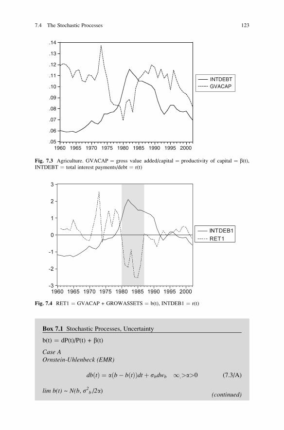
Box 7.1 Stochastic Processes, Uncertainty

b(t) ¼ dP(t)/P(t) + b(t)

Case AOrnstein-Uhlenbeck (EMR)

dbðtÞ ¼ a b� bðtÞð Þdtþ sbdwb 1;>a>0 (7.3/A)

lim b(t) ~ N(b, s2b /2a) (continued)

.05

.06

.07

.08

.09

.10

.11

.12

.13

.14

1960 1965 1970 1975 1980 1985 1990 1995 2000

INTDEBTGVACAP

Fig. 7.3 Agriculture. GVACAP ¼ gross value added/capital ¼ productivity of capital ¼ b(t),INTDEBT ¼ total interest payments/debt ¼ r(t)

Fig. 7.4 RET1 ¼ GVACAP + GROWASSETS ¼ b(t), INTDEB1 ¼ r(t)

7.4 The Stochastic Processes 123

Brownian Motion-Drift (BMD)

rðtÞ ¼ r dtþ sr dwr (7.4/A)

Case BBrownian Motion-Drift (BMD)

bðtÞ ¼ b dtþ sb dwb (7.3/B)

Brownian Motion-Drift (BMD)

rðtÞ ¼ r dtþ sr dwr (7.4/B)

Case C is the reverse of Case A

The mean (b, r) is written without any time index

7.5 Solution and Interpretation of the OptimalDebt/Net Worth

The solution for the optimal debt ratio – the control variable f(t) ¼ L(t)/X(t) –

concerns the maximization of the expected growth rate of net worth, (7.1) subject to

the appropriate stochastic process in Box 7.1. There are other reasonable criteria

functions and stochastic processes. The mathematical techniques for their solution

are discussed in the Chap. 4. Here, I simply state the results. The basic data

underlying the variables in Box 7.2 are discussed in Sect. 7.6. In Sect. 7.7, I explain

the results stated in Box 7.2 using a Mean-Variance analysis. Then I use the results

in discussing the agricultural debt crisis.

The optimal debt/net worth ratio f*(t) ¼ L(t)/X(t) in Box 7.2 varies according to the

three cases (A), (B) and (C) respectively.The asterisk denotes the optimal value. In each

case, the numerator is a return less an interest rate, and the denominator is a variance.

In case (A), (7.5/A), the optimal ratio of debt/net worth f*(t) varies with time.

It is equal to the current value of the return to capital b(t) less the mean rate of

interest r, divided by the variance of the interest rate var (r(t)). In case (B), (7.5/B),the optimal debt/net worth f* is constant. It is equal to the mean return on capital

less the mean interest rate, (b � r), divided by the variance var [b(t) � r(t)], which

contains the covariances. This case is fully analyzed, using dynamic programming,

in Fleming and Stein (2004). Case (C), (7.5/C) is the reverse of case (A). The debt/

net worth ratio f*(t) varies with time. It is equal to the mean return less the currentinterest rate divided by the variance of the return var b(t).


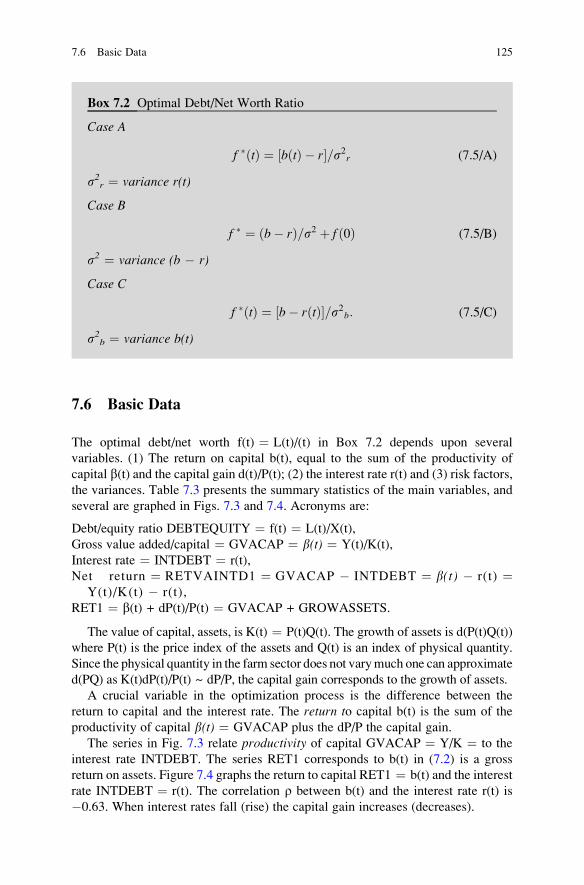
Box 7.2 Optimal Debt/Net Worth Ratio

Case A

f �ðtÞ ¼ bðtÞ � r½ �=s2r (7.5/A)

s2r ¼ variance r(t)

Case B

f � ¼ b� rð Þ=s2 þ f ð0Þ (7.5/B)

s2 ¼ variance (b � r)

Case C

f �ðtÞ ¼ b� rðtÞ½ �=s2b: (7.5/C)

s2b ¼ variance b(t)

7.6 Basic Data

The optimal debt/net worth f(t) ¼ L(t)/(t) in Box 7.2 depends upon several

variables. (1) The return on capital b(t), equal to the sum of the productivity of

capital b(t) and the capital gain d(t)/P(t); (2) the interest rate r(t) and (3) risk factors,the variances. Table 7.3 presents the summary statistics of the main variables, and

several are graphed in Figs. 7.3 and 7.4. Acronyms are:

Debt/equity ratio DEBTEQUITY ¼ f(t) ¼ L(t)/X(t),

Gross value added/capital ¼ GVACAP ¼ b(t) ¼ Y(t)/K(t),

Interest rate ¼ INTDEBT ¼ r(t),

Net return ¼ RETVAINTD1 ¼ GVACAP � INTDEBT ¼ b(t) � r(t) ¼Y(t)/K(t) � r(t),

RET1 ¼ b(t) + dP(t)/P(t) ¼ GVACAP + GROWASSETS.

The value of capital, assets, is K(t) ¼ P(t)Q(t). The growth of assets is d(P(t)Q(t))

where P(t) is the price index of the assets and Q(t) is an index of physical quantity.

Since the physical quantity in the farm sector does not varymuch one can approximate

d(PQ) as K(t)dP(t)/P(t) ~ dP/P, the capital gain corresponds to the growth of assets.

A crucial variable in the optimization process is the difference between the

return to capital and the interest rate. The return to capital b(t) is the sum of the

productivity of capital b(t) ¼ GVACAP plus the dP/P the capital gain.

The series in Fig. 7.3 relate productivity of capital GVACAP ¼ Y/K ¼ to the

interest rate INTDEBT. The series RET1 corresponds to b(t) in (7.2) is a gross

return on assets. Figure 7.4 graphs the return to capital RET1 ¼ b(t) and the interest

rate INTDEBT ¼ r(t). The correlation r between b(t) and the interest rate r(t) is

�0.63. When interest rates fall (rise) the capital gain increases (decreases).

7.6 Basic Data 125

7.7 Mean-Variance Interpretation

Figure 7.5 is Mean-Variance interpretation of the expected growth rate for Case B.

The derivation and technical details are in Chaps. 4 and 5. A similar diagram can be

used for the other cases.

Case B

1=Tð Þ E ln XðTÞ=Xð0Þ½ � ¼ Mean� Risk ¼ expectedgrowthrate: (7.6)

Mean ¼ b� cð Þ þ b� rð Þf (7.6.1)

Risk ¼ 1=2ð Þsb2½ f 2y2 þ 1þ fð Þ2 � 2f 1þ fð Þyr� (7.6.2)

y ¼ sr/sb, r ¼ correlation between (b,r)

There are two terms in the expected growth rate equation (7.6). The first term

Mean is the straight line in Fig. 7.5/Eq. 7.6.1. It is the expected growth rate for any

debt ratio f(t), if there were no risk. The intercept is the appropriate return less the

ratio C/X of (consumption-dividends-distributed profits)/net worth, when there is

no debt. The slope is the appropriate return less the interest rate. The appropriate

measure depends upon the relevant case, (A), (B) or (C). The second term in (7.6) is

graphed as the parabola Risk in Fig. 7.5/Eq. 7.6.2. It is the variance of the change in

net worth.

The expected growth rate of net worth in (7.6) corresponds to the difference

between the straight line Mean and the parabola Risk in Fig. 7.5. In case (B), Mean

and Risk are described by (7.6.1) and (7.6.2) respectively.

Risk

max-expected growth

Mean, Risk

creditordebtor

max-debt

f =L/X =

f*

0

Mean

Fig. 7.5 Mean-variance interpretation of expected growth


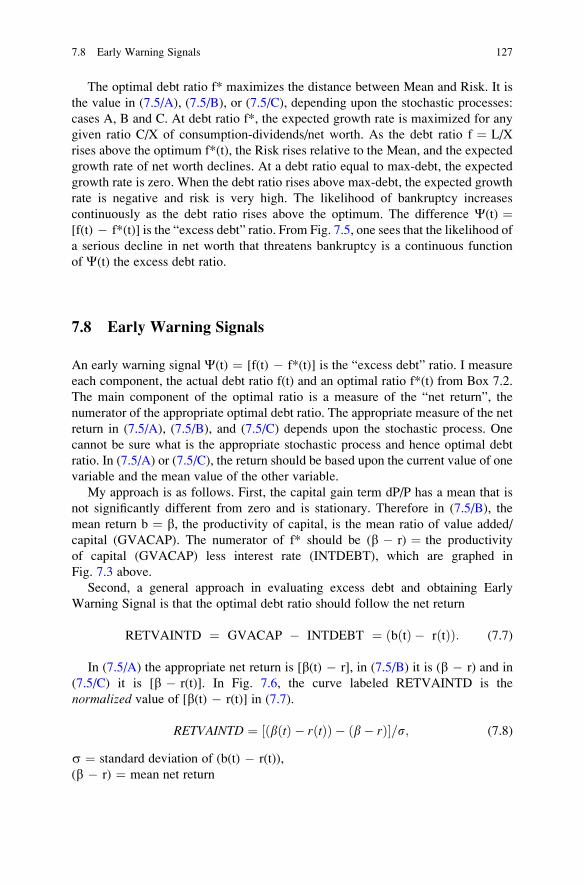
The optimal debt ratio f* maximizes the distance between Mean and Risk. It is

the value in (7.5/A), (7.5/B), or (7.5/C), depending upon the stochastic processes:

cases A, B and C. At debt ratio f*, the expected growth rate is maximized for any

given ratio C/X of consumption-dividends/net worth. As the debt ratio f ¼ L/X

rises above the optimum f*(t), the Risk rises relative to the Mean, and the expected

growth rate of net worth declines. At a debt ratio equal to max-debt, the expected

growth rate is zero. When the debt ratio rises above max-debt, the expected growth

rate is negative and risk is very high. The likelihood of bankruptcy increases

continuously as the debt ratio rises above the optimum. The difference C(t) ¼[f(t) � f*(t)] is the “excess debt” ratio. From Fig. 7.5, one sees that the likelihood of

a serious decline in net worth that threatens bankruptcy is a continuous function

of C(t) the excess debt ratio.

7.8 Early Warning Signals

An early warning signal C(t) ¼ [f(t) � f*(t)] is the “excess debt” ratio. I measure

each component, the actual debt ratio f(t) and an optimal ratio f*(t) from Box 7.2.

The main component of the optimal ratio is a measure of the “net return”, the

numerator of the appropriate optimal debt ratio. The appropriate measure of the net

return in (7.5/A), (7.5/B), and (7.5/C) depends upon the stochastic process. One

cannot be sure what is the appropriate stochastic process and hence optimal debt

ratio. In (7.5/A) or (7.5/C), the return should be based upon the current value of one

variable and the mean value of the other variable.

My approach is as follows. First, the capital gain term dP/P has a mean that is

not significantly different from zero and is stationary. Therefore in (7.5/B), the

mean return b ¼ b, the productivity of capital, is the mean ratio of value added/

capital (GVACAP). The numerator of f* should be (b � r) ¼ the productivity

of capital (GVACAP) less interest rate (INTDEBT), which are graphed in

Fig. 7.3 above.

Second, a general approach in evaluating excess debt and obtaining Early

Warning Signal is that the optimal debt ratio should follow the net return

RETVAINTD ¼ GVACAP � INTDEBT ¼ b tð Þ � r tð Þð Þ: (7.7)

In (7.5/A) the appropriate net return is [b(t) � r], in (7.5/B) it is (b � r) and in

(7.5/C) it is [b � r(t)]. In Fig. 7.6, the curve labeled RETVAINTD is the

normalized value of [b(t) � r(t)] in (7.7).

RETVAINTD ¼ ½ðbðtÞ � rðtÞÞ � ðb� rÞ�=s; (7.8)

s ¼ standard deviation of (b(t) � r(t)),

(b � r) ¼ mean net return

7.8 Early Warning Signals 127

Third, the debt ratio in the optimization is f ¼ L/X ¼ debt/net worth. However,

there is a bias in using this as an empirical measure of an Early Warning Signal

(EWS). The reason is that as net worth EQUITY collapses, this ratio jumps up

violently. For this reason, in empirical work I prefer to use the ratio h ¼ L/Y of debt

(L) to (Y) to net income. Call h the debt ratio. In Fig. 7.6, the normalized value of

the realized debt ratio is:

DEBTNINC ¼ LðtÞ=YðtÞ � L=Yð Þ½ �=s (7.9)

s ¼ standard deviation of [L(t)/Y(t)],

L/Y ¼ mean (L(t)/Y(t))

The optimal debt ratio should either follow RETVAINTD, (Eq. (5A), (5C)) or

be constant (7.5/B). My measure of an excess debt C(t) is the difference between

the normalized curves in Fig. 7.6. Non-optimal debt would occur if the debt ratiowere rising relative to its long term mean when the net return was declining relativeto its mean.

Excess debtCðtÞ ¼ DEBTNINC� RETVAINTD> 0 (7.10)

In Fig. 7.6, the normalized net return fell by almost three standard deviations from

1975 to 1984, but the actual debt ratio rose by about three standard deviations

during that period. Figure 7.7 graphs a normalized value of the excess debt C(t).

It is the normalized difference between DEBTNINC and (GVACAP � INTDEBT).

A large value of normalized deviation C(t) is an EWS of an impending crisis.

This crisis did indeed occur, seen in Fig. 7.2, with the bankruptcies and defaults.

-3

-2

-1

0

1

2

3

4

5

1960 1965 1970 1975 1980 1985 1990 1995 2000

DEBTNINC

RETVAINTD

Fig. 7.6 Agriculture. DEBTNINC ¼ L/Y ¼ Debt/net income; RETVAINTD ¼ GVACAP �INTDEBT ¼ (gross value added/assets � interest rate). Normalized variable ¼ (variable � mean)/

standard deviation


During the periods whenC(t) was small, there were no crises. Figure 7.7 summarizes

the contribution of the SOC approach to provide an EWS of a debt crisis.

A remarkable result is that the same techniques of analysis, SOC, were used to

explain the financial crisis of 2008 and the agricultural crisis of the 1980s. Both

were predictable using the techniques of analysis explained in Chap. 4.

7.9 The S&L Crises

The Agricultural debt crisis and the S&L crisis of the 1980s followed similar

scenarios. The financial debt crisis of 2008 contained the many of the ingredients

of the two financial crises of the 1980s, but involved a national financial structure

rather than a regional one. In each case, the growth of the debt was stimulated by

initial capital gains on assets that increased equity. The productivity of capital was

less than the mean interest rate but the capital gains exceeded the mean interest rate.

Borrowing was based upon the rising equity, so debt service/income rose. Capital

gains (growth in equity) are not sustainable unless they reflect the growth of the

productivity of capital. When the capital gains fell below the interest owed, debts

could not be repaid and a crisis occurred.

In 1979, when it was clear that there was a financial crisis, a bailout or rescue

plan for the S&L industry was undertaken. Between 1975 and 1995, the rescue plan

cost the taxpayers $153 billion – or $320 billion in 2011 prices. I draw upon Curry

and Shibut (2002) and Sungard Ambit Risk (2002). The question is: how could such

a crisis occur in a backwater part of the US financial industry – the S&L industry –

that simply takes retail savings deposits and lends them out in the form of residential

mortgages? Moreover, this sector was regulated by the Federal Savings & Home

Loan Bank Board, which had its own insurance fund to protect depositors, FSLIC.

Fig. 7.7 EXCESS DEBT ¼ DEBTNINC � RETVAINTD, normalized: mean zero, standard

deviation unity. Shaded period, agricultural crisis

7.9 The S&L Crises 129

Equation 7.11 is the framework of the analysis.

dXðtÞ ¼ KðtÞ½dP tð Þ=P tð Þ þ b tð Þ� � rðtÞLðtÞ dt� CðtÞ dt (7.11)

K(t) ¼ P(t)Q(t) ¼ value of assets, L(t) ¼ debt, X(t) ¼ networth ¼ K(t) � L(t),

r(t) ¼ interest rate, dP(t)/P(t) ¼ capital gain or loss, C(t) ¼ consumption.

The inflation and oil price shock in 1979–70 pushed up interest rates, which went

up as high as 16% on government debt. Thereby, a gap opened up for the S&L’s

between the cost of funding their liabilities and the income generated by their

assets, which were long term, fixed rate mortgages. Term [b(t)K(t) � r(t)L(t)]declined, where b(t) is the return on long term fixed rate mortgages, r(t) short

term interest rates. Net worth X(t) often became negative – many of the S&L’s

became insolvent.

New regulations loosened capital requirements and raised the level of insured

deposits. With deregulation and removal of interest rate ceilings, S&L’s had to

compete for funds with the money market funds by offering interest rates r(t) in line

with the market rates. Banks could attract funds by raising interest rates, because

savers knew that their deposits were insured. Banks used these funds to shift away

from conventional mortgages to more risky and higher yielding assets. From the

early 1980s S&L’s began to lend to real estate developers and to invest in real

estate, construction, especially in Texas and Florida. In these regions, property

values, real estate prices P(t) were rising due to the oil price boom. In the farm

regions, the agricultural farm price boom was another factor inducing bank lending/

investment. Large capital gains dP(t)/P(t) were anticipated.

The S&L lending practices had several failings that were repeated by the

financial sector in the 2000–2007 period. There was: (a) an overemphasis on the

up-front fees from advancing commercial real estate loans; (b) a loosening of

underwriting standards which should have ensured creditors that the debtor had

sufficient cash flows from the property development; (c) the loan was unduly large

relative to the property used as security; (d) untrustworthy property value appraisals

that failed to take into account downward movements in property prices in local

markets, including purely speculative assumptions about future capital gains.

The debt L(t) in (7.11) rose. During 1970–1977, there were regional crises

triggered by the collapses in oil prices, prices and property values in the farm

sector. By 1974, the oil price boom was faltering and by 1977 Texas’s oil and real

estate sectors were in deep recession. A similar process of increasing rates of

default and falling collateral values undermined S&L assets around the US until

1992. Texas S&L’s were the worst hit. The crisis was due to the negative value of

term {K(t) [b(t) + dP(t)/P(t)] � r(t)L(t)}.Public awareness of the scale of the S&L crisis was limited into the late 1980s,

despite the well publicized financial scandals. This changed significantly after

President Bush’s speech in February 1979. Congress then passed an act that

substantially restructured the US financial industry regulation and the US taxpayers

would end up paying the bill for the S&L fiasco. The financial market and the Fed in

the 2000–2007 period ignored the lessons of the two crises in the 1980s.


References

Barry, Peter J. and Lindon J. Robison. 2001. Agricultural finance: Credit constraints and

consequences. In Handbook of agricultural economics, eds. B. Gardner and G. Rausser, ch.

10. Amsterdam: Elsevier Science B.V.

Curry, T., and L. Shibut. 2002. The cost of the savings and loan crisis: Truth and consequences.

FDIC Banking Review.Economic Research Service USDA. 2002. Agricultural income and finance outlook/AIS-77/

February 26,2002.

Federal Deposit Insurance Corporation (FDIC). 1997. An examination of the banking crises of the

1980s and early 1990s, history of the eighties – lessons for the future, banking and the

agricultural problems of the 1980s, ch. 7 <www.fdic.gov/bank>.


and debt. Journal of Banking & Finance 28: 979–996.Moss, Charles and Schmitz, Andrew. 2003. Governement policy and farmland markets. Ames:

Iowa State Press.

Sungard Ambit Risk. 2002. US Savings & Loan Crisis.

United States Department of Agriculture (USDA). 2002. Economic research service (ERS), farm

income and balance sheet indicators, 1929–2002, November 26, 2002.

References 131

Chapter 8

The Diversity of Debt Crises in Europe

Abstract The Stability and Growth Pact is seriously incomplete because it only

focuses on government deficits and debt but does not focus upon the external net

debt arising from the excessive accumulation of private external debt as well as

external government debt. The cases of Ireland and Spain differ from Greece,

Portugal and Italy. This chapter provides the underlying analytics for understanding

the debt crises in Europe by drawing on the NATREX model that explains the

simultaneous evolution of the external debt and real exchange rate.

The external debts of the European countries are at the core of the current crises.

Generally, the crises are attributed to government budget deficits in excess of the

values stated in the Stability and Growth Pact (SGP)/Maastricht treaty. Proposals

for reform generally involve increasing the powers of the European Union to

monitor fiscal policies of the national governments and increasing bank regulation.

This chapter explains the inter-country differences in the debt crisis in Europe.

My basic questions in the European context are: In the various countries, how were

“excessive/non sustainable” external debt ratios produced? Were the crises due to

government budget deficits/government dissaving or to private investment less

private saving? What is the mechanism whereby the actions of the public and

private sectors lead to an unsustainable debt burden, defined as an unsustainable

ratio of debt service/GDP? The Stability and Growth Pact/Maastricht Treaty

and the European Union focused upon rules concerning government debt ratios

and deficit ratios. They ignored the problem of “excessive” external debt ratios in

the entire economy that led to a crisis in the financial markets. An austerity policy is

not necessarily an optimal solution for all of the highly indebted countries.

The answers determine to a large extent how one should evaluate proposals for

economic reform to avert future crises.


133

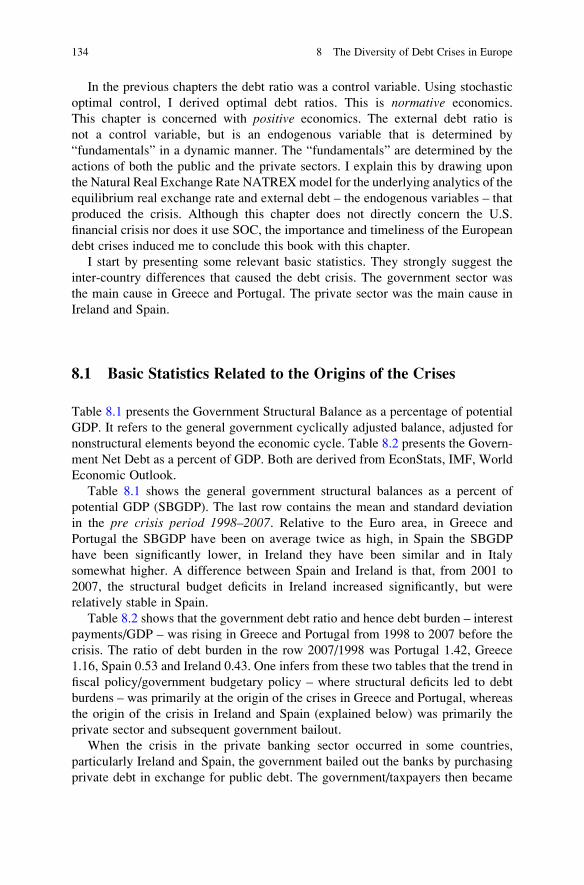
In the previous chapters the debt ratio was a control variable. Using stochastic

optimal control, I derived optimal debt ratios. This is normative economics.

This chapter is concerned with positive economics. The external debt ratio is

not a control variable, but is an endogenous variable that is determined by

“fundamentals” in a dynamic manner. The “fundamentals” are determined by the

actions of both the public and the private sectors. I explain this by drawing upon

the Natural Real Exchange Rate NATREXmodel for the underlying analytics of the

equilibrium real exchange rate and external debt – the endogenous variables – that

produced the crisis. Although this chapter does not directly concern the U.S.

financial crisis nor does it use SOC, the importance and timeliness of the European

debt crises induced me to conclude this book with this chapter.

I start by presenting some relevant basic statistics. They strongly suggest the

inter-country differences that caused the debt crisis. The government sector was

the main cause in Greece and Portugal. The private sector was the main cause in

Ireland and Spain.

8.1 Basic Statistics Related to the Origins of the Crises

Table 8.1 presents the Government Structural Balance as a percentage of potential

GDP. It refers to the general government cyclically adjusted balance, adjusted for

nonstructural elements beyond the economic cycle. Table 8.2 presents the Govern-

ment Net Debt as a percent of GDP. Both are derived from EconStats, IMF, World

Economic Outlook.

Table 8.1 shows the general government structural balances as a percent of

potential GDP (SBGDP). The last row contains the mean and standard deviation

in the pre crisis period 1998–2007. Relative to the Euro area, in Greece and

Portugal the SBGDP have been on average twice as high, in Spain the SBGDP

have been significantly lower, in Ireland they have been similar and in Italy

somewhat higher. A difference between Spain and Ireland is that, from 2001 to

2007, the structural budget deficits in Ireland increased significantly, but were

relatively stable in Spain.

Table 8.2 shows that the government debt ratio and hence debt burden – interest

payments/GDP – was rising in Greece and Portugal from 1998 to 2007 before the

crisis. The ratio of debt burden in the row 2007/1998 was Portugal 1.42, Greece

1.16, Spain 0.53 and Ireland 0.43. One infers from these two tables that the trend in

fiscal policy/government budgetary policy – where structural deficits led to debt

burdens – was primarily at the origin of the crises in Greece and Portugal, whereas

the origin of the crisis in Ireland and Spain (explained below) was primarily the

private sector and subsequent government bailout.

When the crisis in the private banking sector occurred in some countries,

particularly Ireland and Spain, the government bailed out the banks by purchasing

private debt in exchange for public debt. The government/taxpayers then became

134 8 The Diversity of Debt Crises in Europe

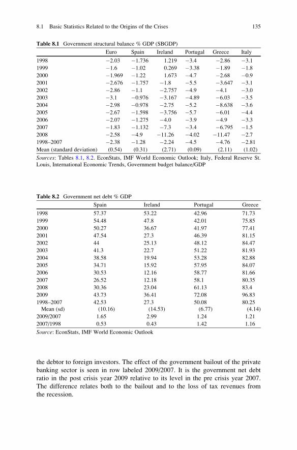
the debtor to foreign investors. The effect of the government bailout of the private

banking sector is seen in row labeled 2009/2007. It is the government net debt

ratio in the post crisis year 2009 relative to its level in the pre crisis year 2007.

The difference relates both to the bailout and to the loss of tax revenues from

the recession.

Table 8.1 Government structural balance % GDP (SBGDP)

Euro Spain Ireland Portugal Greece Italy

1998 �2.03 �1.736 1.219 �3.4 �2.86 �3.1

1999 �1.6 �1.02 0.269 �3.38 �1.89 �1.8

2000 �1.969 �1.22 1.673 �4.7 �2.68 �0.9

2001 �2.676 �1.757 �1.8 �5.5 �3.647 �3.1

2002 �2.86 �1.1 �2.757 �4.9 �4.1 �3.0

2003 �3.1 �0.976 �3.167 �4.89 �6.03 �3.5

2004 �2.98 �0.978 �2.75 �5.2 �8.638 �3.6

2005 �2.67 �1.598 �3.756 �5.7 �6.01 �4.4

2006 �2.07 �1.275 �4.0 �3.9 �4.9 �3.3

2007 �1.83 �1.132 �7.3 �3.4 �6.795 �1.5

2008 �2.58 �4.9 �11.26 �4.02 �11.47 �2.7

1998–2007 �2.38 �1.28 �2.24 �4.5 �4.76 �2.81

Mean (standard deviation) (0.54) (0.31) (2.71) (0.09) (2.11) (1.02)

Sources: Tables 8.1, 8.2. EconStats, IMF World Economic Outlook; Italy, Federal Reserve St.

Louis, International Economic Trends, Government budget balance/GDP

Table 8.2 Government net debt % GDP

Spain Ireland Portugal Greece

1998 57.37 53.22 42.96 71.73

1999 54.48 47.8 42.01 75.85

2000 50.27 36.67 41.97 77.41

2001 47.54 27.3 46.39 81.15

2002 44 25.13 48.12 84.47

2003 41.3 22.7 51.22 81.93

2004 38.58 19.94 53.28 82.88

2005 34.71 15.92 57.95 84.07

2006 30.53 12.16 58.77 81.66

2007 26.52 12.18 58.1 80.35

2008 30.36 23.04 61.13 83.4

2009 43.73 36.41 72.08 96.83

1998–2007

Mean (sd)

42.53

(10.16)

27.3

(14.53)

50.08

(6.77)

80.25

(4.14)

2009/2007 1.65 2.99 1.24 1.21

2007/1998 0.53 0.43 1.42 1.16

Source: EconStats, IMF World Economic Outlook

8.1 Basic Statistics Related to the Origins of the Crises 135

8.2 Crises in Ireland, Spain and Greece

I describe the country experiences by drawing upon the reports of the central banks

and the EEAG (2011). The story is the same for Ireland and Spain, but different in

Greece and Portugal. First, I describe what happened in Ireland and Spain and then

in Greece. In Ireland and Spain the structural government budget deficits were

lower than in the Euro area (Table 8.1). In these countries, the private sector –

housing and banks – was the origin of the debt crisis. Low interest rates, based upon

the assumption that there was neither a default risk nor an exchange risk, led to an

elastic supply of external funds for the Euro area countries. The demand for non-

tradables, in particular housing, was stimulated by low interest rates and growth.

Private investment exceeded private saving, the relative price of non-tradables rose,

which appreciated the real exchange rate, and thereby generated current account

deficits and external debt. In Greece, the current account deficit was attributable

to both the government and the private sectors. Later in this chapter, I use the

NATREX model to explain the underlying analytics of the trajectories of

the external debt and equilibrium real exchange rate, the ratio of domestic/foreign

prices. As the external debt burden rises, the probability of a crisis increases.

8.2.1 Ireland

The Celtic Tiger boom in the late 1980s brought sustained growth in employment,

income and household formation. Ireland’s becoming a founding member of the

Euro zone brought a sustained fall in nominal interest rates, which in turn led to

higher asset valuations. The growing construction boomwas financed by Irish banks

which in turn were financed by external financial markets where inexpensive funds

were available. In the last 4 years of the boom from 2003 onwards banks competed

aggressively in the mortgage markets with little regard for the creditworthiness of

the mortgagors. At the end of 2003, net indebtedness of Irish banks to the world was

over 10% GDP. By 2008, borrowing mainly for property jumped to over 60% GDP.

Even before the failure of Lehman Brothers (Sep. 2008) Irish residential

properties had been falling for more than 18 months. At no point throughout the

period, even as the crisis neared, did the Central bank and Financial Services

Authority of Ireland staff believe that any of the institutions were facing serious

underlying difficulties let alone insolvency problems.

When the crisis occurred, the collapse of construction and the fall in property

prices led to the insolvency of banks. Their net worth vanished. The state took large

equity stakes in most banks and issued government guaranteed bonds. Although

Ireland’s public debt immediately prior to the crisis was low (Table 8.2), the fiscal

deficit and public sector borrowing surged. The structural budget deficit increased

significantly during the period 2000–2007. It went from a surplus of 1.67% in year

2000 to a deficit of 7.3% in 2007. A reason for the surge in the deficit was the

collapse of tax revenues in 2008–2009 due to the collapse of the housing sector.


8.2.2 Spain

Throughout the 1989–2006 period, demand in the Spanish economy grew at 4.7%

pa whereas output expanded by 3.8% pa, driven by immigration and increased labor

force participation. There was scarcely any growth in productivity. Since absorp-

tion exceeded production, external debt grew and the real exchange rate – equal to

the nominal rate times relative prices – appreciated. Insofar as the nominal

exchange rate was fixed in the Euro area, Spanish prices and costs rose relative to

the rest of the Euro area. The Spanish economy lost competitiveness. Unlike

previous expansions, the resort to financing was not chiefly by the public sector

which reduced its debt throughout the period. See Table 8.2. Instead it was the

Spanish households and firms that swiftly increased their debts. The real estate

market propelled the expansion. Housing prices climbed from an average rate of

1% pa between 1995 and 1997 to 18% pa between 2003 and 2004, or an annual

average increase between 1995 and 2007 of 10%.

What facilitated the growth in the debt was the availability of cheap credit in the

international financial markets. See EEAG Fig. 4.12 for the spread between Spanish

and German 10 year bonds, based upon Reuters Ecowin. As a result, the Spanish

economy, which needed virtually no foreign funding in 1996, became a borrower.

In 2008 total net borrowing from the rest of the world was 9.1% GDP.

When housing prices fell, the banks – which financed the housing sector – were

unable to repay their loans to the international lenders. Governments responded

forcefully to the intensification of the financial crisis. At first, measures had focused

on the selective bailout of ailing banks, supplementing the actions of central banks

to prevent liquidity problems in the banking sector from becoming insolvency

problems. However, the risks of financial collapse and the increasingly evident

and heightened prospect of global recession led to the widespread approval of plans

to support the financial sector and to boost aggregate demand via fiscal stimulus.

The breadth of the measures adopted and the volume of resources mobilized were

on an unprecedented scale. The government structural deficit in Spain was rela-

tively constant during the period 2000–2007. The effect of the crisis raised the ratio

of government debt 2009/2007 to 1.65 (Table 8.2).

8.2.3 Greece’s External Debt

The crucial variable leading to a debt crisis is the external debt/GDP. The change in

the external debt is the current account deficit. These variables are presented in

Tables 8.5 and 8.6 for five countries and the Euro area. Both the government sector

and the private sector can produce growth of the external debt. The current account

deficit is equal to social investment less social saving (I � S), where social refers to

the sum of the private and government sectors. Alternatively, the current account

8.2 Crises in Ireland, Spain and Greece 137

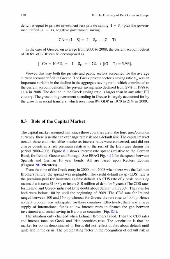
deficit is equal to private investment less private saving (I � Sp) plus the govern-

ment deficit (G � T), negative government saving.

� CA ¼ I� Sð Þ ¼ I� Sp� �þ G� Tð Þ

In the case of Greece, on average from 2000 to 2008, the current account deficit

of 10.6% of GDP can be decomposed as

�CA ¼ 10:6%½ � ¼ I� Sp� � ¼ 4:7%� �þ G� Tð Þ ¼ 5:9%½ �:

Viewed this way both the private and public sectors accounted for the average

current account deficit in Greece. The Greek private sector’s saving ratio Sp was an

important variable in the decline in the aggregate saving ratio, which contributed to

the current account deficits. The private saving ratio declined from 27% in 1988 to

11% in 2008. The decline in the Greek saving ratio is larger than in any other EU

country. The growth in government spending in Greece is largely accounted for by

the growth in social transfers, which rose from 8% GDP in 1970 to 21% in 2009.

8.3 Role of the Capital Market

The capital market assumed that, since these countries are in the Euro area/common

currency, there is neither an exchange rate risk nor a default risk. The capital market

treated these countries alike insofar as interest rates were concerned, and did not

charge countries a risk premium relative to the rest of the Euro area during the

period 2000–2008. Figure 8.1 shows interest rate spreads relative to the German

Bund, for Ireland, Greece and Portugal. See EEAG Fig. 4.12 for the spread between

Spanish and German 10 year bonds. All are based upon Reuters Ecowin

(Plagnol 2010/Reuters).

From the time of the Greek entry in 2000 until 2008 when there was the Lehman

Brothers failure, the spread was negligible. The credit default swap (CDS) rate is

the premium paid for insurance against default. (A CDS rate of y basis points bpmeans that it costs $1,000y to insure $10 million of debt for 5 years.) The CDS rates

for Ireland and Greece indicated little doubt about default until 2009. The rates for

both were below 100 bp until the beginning of 2009. The CDS rate for Ireland

ranged between 100 and 150 bp whereas for Greece the rate rose to 400 bp. Hence

no debt problem was anticipated for these countries. Effectively, there was a large

supply of international funds at low interest rates to finance the gap between

investment and social saving in Euro area countries (Fig. 8.1).

The situation only changed when Lehman Brothers failed. Then the CDS rates

and interest rates on Greek and Irish securities rose. The conclusion is that the

market for bonds denominated in Euros did not reflect doubts about default until

quite late in the crisis. The precipitating factor in the recognition of default risk in


Europe was the failure of Lehman Brothers. By then it was too late. C. Fischer

found that the rescue of Bear Stearns in March 2008 seems to mark a change in

market perceptions of sovereign bond risk. The government bonds of some

countries lost their former role as a safe haven.

The ignoring of default risk stands in contrast with the U.S. experience where,

despite having a common currency, the market evaluates municipalities according

to the default risk. Neither the Treasury nor the Federal Reserve intervenes in the

fiscal policies of the municipalities nor contemplates bailouts when they are

experiencing difficulties in servicing their debts. Table 8.3 presents the distribution

of ratings, and hence interest rates that the capital market charges the various U.S.

municipalities. In the U.S. the fiscal discipline comes from the markets and notfrom the government.

Table 8.3 United States municipal rating distribution 1970–2000

Bond rating Percent (%) of municipalities

AAA 3.15

Aa 11.5

A 54.42

Baa 29.9

Ba 0.8

B 0.13

Caa-C 0.02

Special comment: Moody’s U.S. Municipal Bond Rating Scale, Nov. 2002

Fig. 8.1 Interest rate spreads versus the Bund

8.3 Role of the Capital Market 139

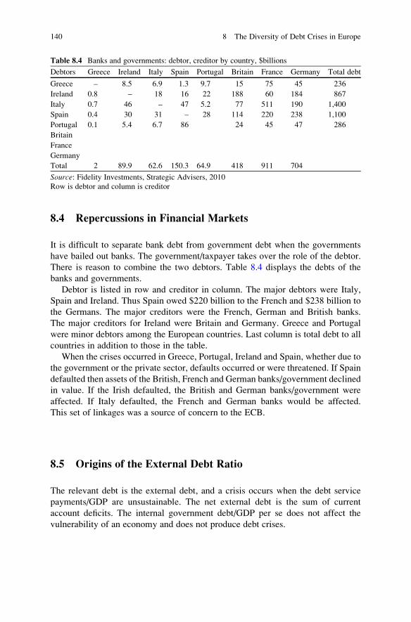
8.4 Repercussions in Financial Markets

It is difficult to separate bank debt from government debt when the governments

have bailed out banks. The government/taxpayer takes over the role of the debtor.

There is reason to combine the two debtors. Table 8.4 displays the debts of the

banks and governments.

Debtor is listed in row and creditor in column. The major debtors were Italy,

Spain and Ireland. Thus Spain owed $220 billion to the French and $238 billion to

the Germans. The major creditors were the French, German and British banks.

The major creditors for Ireland were Britain and Germany. Greece and Portugal

were minor debtors among the European countries. Last column is total debt to all

countries in addition to those in the table.

When the crises occurred in Greece, Portugal, Ireland and Spain, whether due to

the government or the private sector, defaults occurred or were threatened. If Spain

defaulted then assets of the British, French and German banks/government declined

in value. If the Irish defaulted, the British and German banks/government were

affected. If Italy defaulted, the French and German banks would be affected.

This set of linkages was a source of concern to the ECB.

8.5 Origins of the External Debt Ratio

The relevant debt is the external debt, and a crisis occurs when the debt service

payments/GDP are unsustainable. The net external debt is the sum of current

account deficits. The internal government debt/GDP per se does not affect the

vulnerability of an economy and does not produce debt crises.

Table 8.4 Banks and governments: debtor, creditor by country, $billions

Debtors Greece Ireland Italy Spain Portugal Britain France Germany Total debt

Greece – 8.5 6.9 1.3 9.7 15 75 45 236

Ireland 0.8 – 18 16 22 188 60 184 867

Italy 0.7 46 – 47 5.2 77 511 190 1,400

Spain 0.4 30 31 – 28 114 220 238 1,100

Portugal 0.1 5.4 6.7 86 24 45 47 286

Britain

France

Germany

Total 2 89.9 62.6 150.3 64.9 418 911 704

Source: Fidelity Investments, Strategic Advisers, 2010

Row is debtor and column is creditor


8.5.1 Current Account/GDP and Net External Debt/GDP

Table 8.5 describes the current account/GDP in the Euro area and the five countries.

The net external debt is the sum of current account deficits. The steady trend in

current account deficits led to a growing external debt.

Table 8.6 describes the net external debt/GDP and the general government

external debt/GDP, as of the end of 2009. The net external debt/GDP in column 1

is the key to understanding the crises in Europe. It is equal to the debt like securities

liabilities less the corresponding asset claims. Column 2 is the general government

net external debt/GDP. The levels and trends in the current account deficits were

greatest in Greece and Portugal.

Looking at Germany one sees the difference between the two measures.

Germany is a net creditor concerning the net external debt, whereas it has a generalgovernment net debt/GDP similar to Spain and higher than Italy. Portugal, Greece

and Spain have the highest net external debt/GDP, which combines the private and

public sectors. Italy does not have a high net external debt/GDP. Therefore, the

Table 8.5 Current account/GDP

Obs Euro area Greece Ireland Spain Italy Portugal

1998 �2.8 0.8 �1.2 1.6 �6.8

1999 �0.59 �5.6 0.3 �2.9 0.7 �8.8

2000 �1.35 �7.8 �0.4 �4.0 �0.5 �10.4

2001 �1.06 �7.3 �0.6 �3.9 �0.1 �10.3

2002 0.66 �6.8 �1.0 �3.3 �0.8 �8.23

2003 �0.08 �6.5 0.0 �3.5 �1.3 �6.4

2004 0.78 �5.8 �0.6 �5.3 �0.9 �8.3

2005 0.02 �7.6 �3.5 �7.4 �1.7 �10.3

2006 �0.56 �11.3 �3.6 �9.0 �2.6 �10.7

2007 0.13 �14.5 �5.3 �10.0 �2.4 �10.4

2008 �1.83 �14.7 �5.6 �9.7 �2.9 �12.6

2009 �1.24 �11.4 �3.0 �5.5 �2.1 �10.2

2010 �0.81 �10.5 �0.3 �5.5 �3.5

Source: Federal Reserve St. Louis, International Economic Trends; Portugal, World Bank

Table 8.6 External debt position end 2009

Country Net external debt/GDP General government net external debt/GDP

Portugal 88.6% 74.4%

Greece 82.5 78.9

Spain 80.6 47.3

Ireland 75.1 70.6

Italy 37.3 42.9

Germany �21.7 48.5

Source: Ricardo Cabral, The PIGS’ external debt problem, VOX, May 8, 2010

Negative value is creditor

8.5 Origins of the External Debt Ratio 141

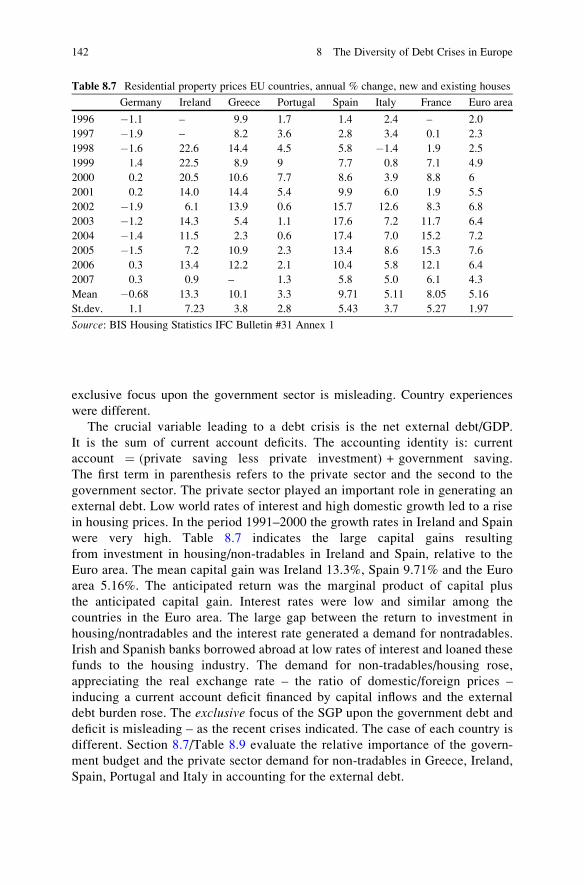
exclusive focus upon the government sector is misleading. Country experiences

were different.

The crucial variable leading to a debt crisis is the net external debt/GDP.

It is the sum of current account deficits. The accounting identity is: current

account ¼ (private saving less private investment) + government saving.

The first term in parenthesis refers to the private sector and the second to the

government sector. The private sector played an important role in generating an

external debt. Low world rates of interest and high domestic growth led to a rise

in housing prices. In the period 1991–2000 the growth rates in Ireland and Spain

were very high. Table 8.7 indicates the large capital gains resulting

from investment in housing/non-tradables in Ireland and Spain, relative to the

Euro area. The mean capital gain was Ireland 13.3%, Spain 9.71% and the Euro

area 5.16%. The anticipated return was the marginal product of capital plus

the anticipated capital gain. Interest rates were low and similar among the

countries in the Euro area. The large gap between the return to investment in

housing/nontradables and the interest rate generated a demand for nontradables.

Irish and Spanish banks borrowed abroad at low rates of interest and loaned these

funds to the housing industry. The demand for non-tradables/housing rose,

appreciating the real exchange rate – the ratio of domestic/foreign prices –

inducing a current account deficit financed by capital inflows and the external

debt burden rose. The exclusive focus of the SGP upon the government debt and

deficit is misleading – as the recent crises indicated. The case of each country is

different. Section 8.7/Table 8.9 evaluate the relative importance of the govern-

ment budget and the private sector demand for non-tradables in Greece, Ireland,

Spain, Portugal and Italy in accounting for the external debt.

Table 8.7 Residential property prices EU countries, annual % change, new and existing houses

Germany Ireland Greece Portugal Spain Italy France Euro area

1996 �1.1 – 9.9 1.7 1.4 2.4 – 2.0

1997 �1.9 – 8.2 3.6 2.8 3.4 0.1 2.3

1998 �1.6 22.6 14.4 4.5 5.8 �1.4 1.9 2.5

1999 1.4 22.5 8.9 9 7.7 0.8 7.1 4.9

2000 0.2 20.5 10.6 7.7 8.6 3.9 8.8 6

2001 0.2 14.0 14.4 5.4 9.9 6.0 1.9 5.5

2002 �1.9 6.1 13.9 0.6 15.7 12.6 8.3 6.8

2003 �1.2 14.3 5.4 1.1 17.6 7.2 11.7 6.4

2004 �1.4 11.5 2.3 0.6 17.4 7.0 15.2 7.2

2005 �1.5 7.2 10.9 2.3 13.4 8.6 15.3 7.6

2006 0.3 13.4 12.2 2.1 10.4 5.8 12.1 6.4

2007 0.3 0.9 – 1.3 5.8 5.0 6.1 4.3

Mean �0.68 13.3 10.1 3.3 9.71 5.11 8.05 5.16

St.dev. 1.1 7.23 3.8 2.8 5.43 3.7 5.27 1.97

Source: BIS Housing Statistics IFC Bulletin #31 Annex 1


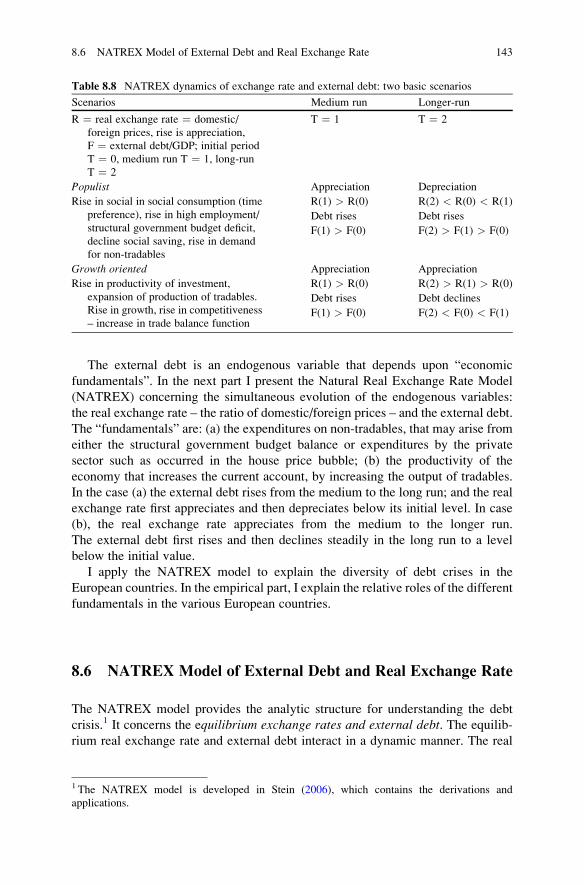
The external debt is an endogenous variable that depends upon “economic

fundamentals”. In the next part I present the Natural Real Exchange Rate Model

(NATREX) concerning the simultaneous evolution of the endogenous variables:

the real exchange rate – the ratio of domestic/foreign prices – and the external debt.

The “fundamentals” are: (a) the expenditures on non-tradables, that may arise from

either the structural government budget balance or expenditures by the private

sector such as occurred in the house price bubble; (b) the productivity of the

economy that increases the current account, by increasing the output of tradables.

In the case (a) the external debt rises from the medium to the long run; and the real

exchange rate first appreciates and then depreciates below its initial level. In case

(b), the real exchange rate appreciates from the medium to the longer run.

The external debt first rises and then declines steadily in the long run to a level

below the initial value.

I apply the NATREX model to explain the diversity of debt crises in the

European countries. In the empirical part, I explain the relative roles of the different

fundamentals in the various European countries.

8.6 NATREX Model of External Debt and Real Exchange Rate

The NATREX model provides the analytic structure for understanding the debt

crisis.1 It concerns the equilibrium exchange rates and external debt. The equilib-rium real exchange rate and external debt interact in a dynamic manner. The real

Table 8.8 NATREX dynamics of exchange rate and external debt: two basic scenarios

Scenarios Medium run Longer-run

R ¼ real exchange rate ¼ domestic/

foreign prices, rise is appreciation,

F ¼ external debt/GDP; initial period

T ¼ 0, medium run T ¼ 1, long-run

T ¼ 2

T ¼ 1 T ¼ 2

Populist Appreciation Depreciation

Rise in social in social consumption (time

preference), rise in high employment/

structural government budget deficit,

decline social saving, rise in demand

for non-tradables

R(1) > R(0) R(2) < R(0) < R(1)

Debt rises Debt rises

F(1) > F(0) F(2) > F(1) > F(0)

Growth oriented Appreciation Appreciation

Rise in productivity of investment,

expansion of production of tradables.

Rise in growth, rise in competitiveness

– increase in trade balance function

R(1) > R(0) R(2) > R(1) > R(0)

Debt rises Debt declines

F(1) > F(0) F(2) < F(0) < F(1)

1 The NATREX model is developed in Stein (2006), which contains the derivations and

applications.

8.6 NATREX Model of External Debt and Real Exchange Rate 143

rate is defined as the nominal exchange rate times relative domestic/foreign prices.

In a monetary union, the nominal exchange rate is fixed at unity and the actual real

exchange rate varies due to changes in relative prices. In a floating exchange rate

regime, both the nominal exchange rate and relative prices can lead to adjustments

in the actual real rate. The only difference from our point of view is that the

adjustment of the actual real exchange rate to the equilibrium will be faster, and

with less adverse effects upon growth, when the exchange rate floats, because the

nominal exchange rate is more flexible than relative prices.

The concept and measure of the equilibrium exchange rate depends upon

the time horizon and the underlying model. Several reasons have been cited in

the literature why it is important to estimate equilibrium exchange rates. First, thereare significant and sustained movements in exchange rates. These movements

affect the competitiveness of the economies and their macroeconomic stability.

One wants to know whether these movements are ephemeral or whether they are

responding to “real fundamentals”. This information is important because the

answer has implications for rational macroeconomic policy. If the depreciation of

an exchange rate is due to a depreciation of its equilibrium value, then exchange

market intervention or a restrictive monetary policy designed to offset the depreci-

ation is counterproductive.

Second, in the case of monetary unions such as the Euro area, it is important to

know how a potential entrant should select its exchange rate. An “overvalued” rate

will depress growth, increase the external debt and produce problems such as beset

the eastern part of Germany. An “undervalued” rate will generate inflationary

pressures. The measure of “over-valuation” and “under-valuation” must contain

an explicit measure of an “equilibrium” real exchange rate.

The literature of “equilibrium exchange rates” was given great impetus by John

Williamson’s influential book (1994). The logic of this approach goes back to

Ragnar Nurske’s article. The “equilibrium” exchange rate is the exchange rate

that is associated with both external and internal balance. Anticipations, speculative

capital movements and changes in reserves are excluded from the concept of an

equilibrium exchange rate, which is where the exchange rate is heading.

The NATREX model of equilibrium exchange rates generalizes the work of

Williamson and Nurske. It is a Neoclassical growth model, whose underlying

equations are based upon an intertemporal optimization by the private sector, but

not the government whose decisions are political.

The NATREX explains the fundamental determinants of the medium run equi-

librium and the dynamic trajectory of the real exchange rate and the external debt to

the long run equilibrium. In the medium run equilibrium there are both internal and

external balances. In both the medium run and longer run the NATREX equilibrium

real exchange rate satisfies Eq. 8.1, subject to constraints. The constraints are thatthere is internal balance, where the rate of capacity utilization is at its longer term

mean, and external balance where the real rates of interest at home and abroad are

equal, there are neither changes in reserves, nor speculative capital flows based

upon anticipations. The equilibrium real exchange rate is the mean of a distribution,

which is based upon real fundamentals. The mean will vary over time due


to endogenous changes in capital and external debt, as well as changes in the

exogenous real fundamentals. Deviations from this mean are produced by specula-

tive factors involving anticipations, cyclical factors, lags in adjustment, and interest

rate differentials. These disequilibrium elements average out to zero. These

deviations produce considerable variation but their effects are ephemeral.

All of the authors who take the equilibrium real exchange rate approach

use Eq. 8.1 to determine the exchange rate. Investment less saving (It � St) plus

the current account is equal to zero. Investment less saving is the non-speculative

capital inflow. The current account (Bt � rtFt) is the trade balance Bt less transfers of

interest and dividends rtFt. The net external debt is Ft and rt is the “interest/dividend”

rate. The international investment position consists of equity, portfolio investment

and direct investment. The debt Ft is the negative of the net international investment

position. Measure investment, saving and the debt as fractions of the GDP.

½ðIt � StÞ þ ðBt � rtFtÞ� ¼ 0 (8.1)

The main differences among authors concern their treatment of the two terms.

Some work with a concept of what is a “sustainable” current account such that the

debt does not “explode”. Their estimates are subjective, so their equilibrium

exchange rate is an arbitrary normative measure. The NATREX approach is quite

different in several respects. First, it is positive economics. The “fundamentals”

determine the trajectories of the external debt and equilibrium real exchange rate.

Second, it is a dynamic analysis. The endogenous current account generates an

evolving external debt, which feeds back into the medium run equation 8.1. A tra-

jectory to longer run equilibrium is generated.

The dynamics of the debt/GDP ratio Ft is Eq. 8.2, where g is the growth rate.

The current account deficit is the change in the external debt. The real exchange rate

affects the trade balance B in Eq. 8.1, and the trade balance affects the evolution of

the actual debt ratio in Eq. 8.2. There is a dynamic interaction between the

endogenous real exchange rate and debt ratio.

dFt=dt ¼ It � Stð Þ � gtFt ¼ rtFt � Btð Þ � gtFt ¼ rt � gtð ÞFt � Bt (8.2)

In longer run equilibrium, the debt ratio stabilizes at a value that satisfies Eq. 8.3.The trade balance Bt is sufficient to finance the interest plus dividend transfer on the

debt net of growth (rt � gt)Ft. A negative debt is net foreign assets.

rt � gtð ÞFt � Bt ¼ 0: (8.3)

The longer-run equilibrium real exchange rate Rt* and debt/GDP ratio Ft* are

endogenous variables that satisfy both Eqs. 8.1 and 8.3. They are written as (8.4)

and (8.5) to indicate that they both depend upon the real fundamentals Zt.

Rt� ¼ R Ztð Þ (8.4)


Ft� ¼ F Ztð Þ: (8.5)

The dynamic stock-flow model equations 8.1, 8.2 and 8.3 is the NATREX

model, which is an acronym for the Natural Real Exchange Rate. This is a model

of positive economics. The derivation of the underlying equations is in Stein (2006,Chap. 4). The literature associated with Williamson’s FEER uses Eq. 8.1, is

normative and does not contain the dynamic interactions, Eqs. 8.2 and 8.3.

8.6.1 Populist and Growth Scenarios

The NATREX model is a technique of analysis. The purpose of the model is to

understand the effects of policies and external disturbances upon the trajectories of

the equilibrium real exchange rate Rt and equilibrium external debt ratio Ft, which

depend upon the vector of fundamentals Zt. Insofar as the fundamentals vary over

time, the equilibrium real exchange rate and debt ratio will vary over time, as

indicated in Eqs. 8.4 and 8.5. The logic and insights of the NATREX model can be

summarized in two scenarios. Each scenario concerns different elements in the

vector Zt of the fundamentals, and has different effects upon the equilibriumtrajectories of the real exchange rate NATREX and of the external debt. NATREX

analysis concerns the equilibrium real exchange rate and it is neither the actual realexchange rate nor the optimal exchange rate that would lead to the optimal debtratio. Table 8.8 summarizes the differences between the two scenarios in the

medium and the long run.

The first scenario, called the Populist scenario, involves a decline in the ratio of

social saving/GDP. This could occur when the government incurs high-employ-

ment budget deficits, lowers tax rates that raise consumption, or offers low interest

rate loans for the production of non-tradable goods. This represents a rise in the

consumption ratio/decline in the saving ratio, a shift in the S function in Eqs. 8.1

and 8.2. These Populist expenditures are designed to raise the standards of con-

sumption/quality of life for the present generation.

The second scenario, called the Growth scenario, involves policies designed to

raise the productivity of capital, increase the competitiveness of the economy, and

increase the supply of traded goods. Growth policies improve the allocation of

resources and bring the economy closer to the boundary of an expanding production

possibility curve.

The stories behind the dynamics are as described by Figs. 8.2, 8.3 and Table 8.8.

Curve SI in Fig. 8.2 is saving less investment (S � I)(t). It is positively related to

the real exchange rate, because a rise in domestic/foreign prices adversely affects

investment (see Stein 2006, Chap. 4). The curve labeled CA(t) is the current

account function (Bt � rtFt), which is negatively related to the real exchange

rate, because a rise in domestic/foreign prices adversely affects the trade balance.

Initial equilibrium is R ¼ R(0) and CA ¼ 0.


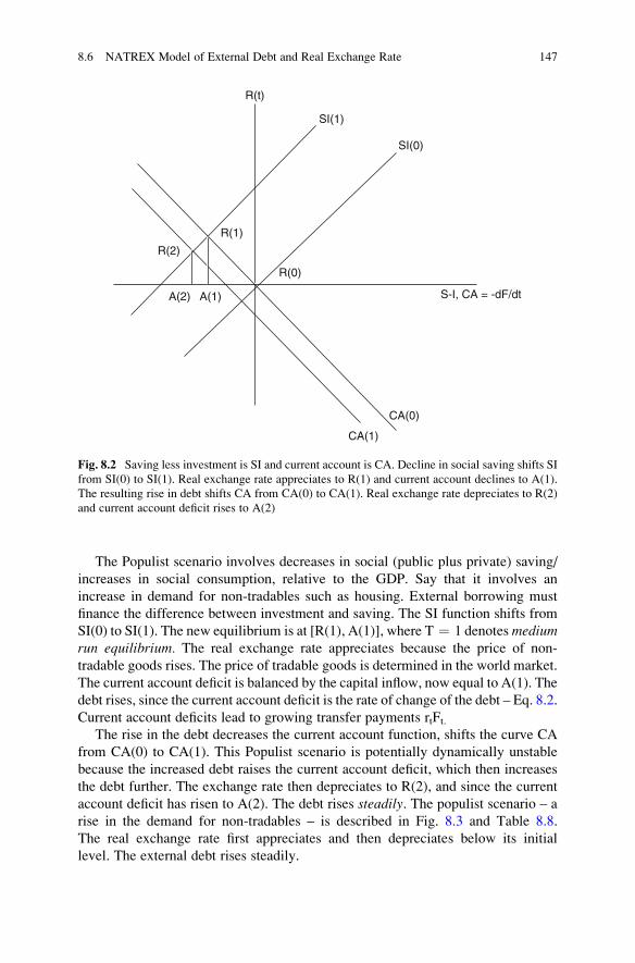
The Populist scenario involves decreases in social (public plus private) saving/

increases in social consumption, relative to the GDP. Say that it involves an

increase in demand for non-tradables such as housing. External borrowing must

finance the difference between investment and saving. The SI function shifts from

SI(0) to SI(1). The new equilibrium is at [R(1), A(1)], where T ¼ 1 denotesmediumrun equilibrium. The real exchange rate appreciates because the price of non-

tradable goods rises. The price of tradable goods is determined in the world market.

The current account deficit is balanced by the capital inflow, now equal to A(1). The

debt rises, since the current account deficit is the rate of change of the debt – Eq. 8.2.

Current account deficits lead to growing transfer payments rtFt.The rise in the debt decreases the current account function, shifts the curve CA

from CA(0) to CA(1). This Populist scenario is potentially dynamically unstable

because the increased debt raises the current account deficit, which then increases

the debt further. The exchange rate then depreciates to R(2), and since the current

account deficit has risen to A(2). The debt rises steadily. The populist scenario – a

rise in the demand for non-tradables – is described in Fig. 8.3 and Table 8.8.

The real exchange rate first appreciates and then depreciates below its initial

level. The external debt rises steadily.

R(1)

R(0)

SI(1)

SI(0)

S-I, CA = -dF/dt

CA(0)

CA(1)

R(t)

R(2)

A(2) A(1)

Fig. 8.2 Saving less investment is SI and current account is CA. Decline in social saving shifts SI

from SI(0) to SI(1). Real exchange rate appreciates to R(1) and current account declines to A(1).

The resulting rise in debt shifts CA from CA(0) to CA(1). Real exchange rate depreciates to R(2)

and current account deficit rises to A(2)


Stability can only occur if the rise in the debt, which lowers net worth equal to

capital less debt, reduces social consumption/raises social saving. Thereby, saving

less investment rises. Long-run equilibrium (denoted by T ¼ 2) is reached at a

higher debt F(2) > F(0) and a depreciated real exchange rate R(2) < R(0).

The longer-run depreciation of the exchange rate R(2) < R(0) can be understood

from Eq. 8.3. The debt is higher than initially. Therefore, the trade balance B(2)

must be higher than initially to generate the foreign exchange to service the higher

transfers rtF(2). The mean interest rate must exceed the mean growth rate if the

expected present value of future income is finite. The real exchange rate must

depreciate to R(2) < R(0) in order to raise the trade balance to B(2).

TheGrowth scenario is summarized in the lower half of Table 8.8. The perturba-

tion is a rise in the productivity of investment and an expansion of the production of

tradables. Investment rises because of the rise in the rate of return. The difference

between investment and saving is financed by a capital inflow. S-I shifts from S(0) to

S(1) in Fig. 8.2. The exchange rate appreciates to R(1) > R(0) which reduces the

trade balance and initially produces a current account deficit A(1). The current

account deficit raises the debt. The trade deficit provides the resources to

finance capital formation, which raises the growth rate and the competitiveness of

the economy.

F(t)

R(t), F(t)

0 time

R(t)

Fig. 8.3 Populist scenario: initial R(0), F(0) at origin. Rise in social consumption, increase

demand for non-tradables generates trajectory R(t) for the real exchange rate and F(t) for the

external debt. In the Growth scenario, the trajectories for the real exchange rate and external debt

trajectory are reversed


The investment in the tradables sector increases the trade balance functionB ¼ B(R;Z). The B function, which relates the value of the trade balance to the

real exchange rate R, increases with a rise in the overall productivity/competitive-

ness of the economy. For example, the reallocation of resources leads to the

production of higher quality/value goods that can compete in the world market.

The medium run effects are the same as those in the populist scenario, but the

trajectories to longer-run equilibrium differ. The crucial aspect implied by

the Growth Scenario is that the economy is more competitive. At exchange rate R

(1), the trade balance function CA increases, shifts to the right. The real exchangerate appreciates and there are now current account surpluses, excess of saving overinvestment. As a result, the debt then declines to a new equilibrium F(2) < F(0).

The trajectory of the debt is not monotonic. The net effect in the longer-run can be

understood from Eq. 8.3. The debt is lower, the growth rate is higher and the trade

balance function B has shifted to the right. The long-run equilibrium exchange ratemust appreciate to reduce B to equal the lower value of (r � g)F*.

The dynamic process in the Growth scenario is summarized in the lower

half of Table 8.8. The real exchange rate appreciates steadily to a higher level

R(2) > R(1) > R(0). The external debt reaches a maximum and then declines to

F(2) < F(0) < F(1). In Fig. 8.3, the curves are reversed.

8.7 NATREX Analysis of the European Situation

I analyze the European experiences within the framework of the NATREX model.

Summary Table 8.9 shows that over the period 1998–2010, there were very large

current account deficits in Greece, Portugal and Spain, relative to the Euro area.

Thereby the external debts of these countries rose. What produced the current

account deficits? They were due to what the NATREX model calls the Populist

Scenario: a decline in government saving and/or a rise in demand for non-tradables.

The role of the government sector is described in the row labeled government

balance. The largest government deficits were in Greece, Portugal and Italy. Hence

one concludes that in Greece, Portugal and Italy, the current account deficits were

significantly produced by high government consumption/low government saving.

In Spain and Ireland, the government sector was not the major cause of a decline

in social saving/rise in social consumption. It was the increase in the demand for

non-tradables/housing. This is reflected in the row labeled House Price appreciation.

In Ireland, Spain and Greece, there was a significant rise in the demand for non-

tradables relative to the Euro area.

The movement of the real exchange rate, equal to the ratio of domestic prices

relative to the Euro area, is reflected in the row labeled GDP deflator. In all of the

countries, both the government sector and the rise in the demand for non-tradables

by the private sector led to an appreciation of the real exchange rate, current

account deficits and the growth in the external debt ratio dFt/dt. The SI curve

shifted from SI(0) to SI(1) in Fig. 8.2 changing the medium run equilibrium to

8.7 NATREX Analysis of the European Situation 149

Tab

le8.9

Summarydata1998–2010

Euro

area

Greece

Ireland

Spain

Portugal

Italy

Currentaccount/GDP

Meanm

=�0

.26

m=�8

.6m

=�1

.75

m=�5

.4m

=�9

.45

m=�1

.7

St.dev.=0.85

sd=3.5

s=2.16

s=2.8

s=1.78

s=1.47

Gov’tbalance

m=�2

.38

m=�4

.76

m=�2

.24

m=�1

.28

m=�4

.5m

=�3

.16

s=0.54

s=2.11

s=2.7

s=0.31

s=0.09

s=1.27

House

price

appreciation,percentchange

m=5.16

m=10.1

m=13.3

m=9.71

m=3.3

m=5.11

s=1.97

s=3.8

s=7.24

s=5.43

s=2.8

s=3.7

GDPdeflator,percentchange

m=1.7

m=3.23

m=2.45

m=3.1

m=2.67

m=2.35

s=0.59

s=0.84

s=3.21

s=1.35

s=1.04

s=0.72

Growth,percentchange

m=1.6

m=2.7

m=4.2

m=2.7

m=1.52

m=0.72

s=2.0

s=2.8

s=5.1

s=2.4

s=2.06

s=2.14

Source:Federal

ReserveSt.Louis,International

Economic

Trends,Tables8.1,8.3


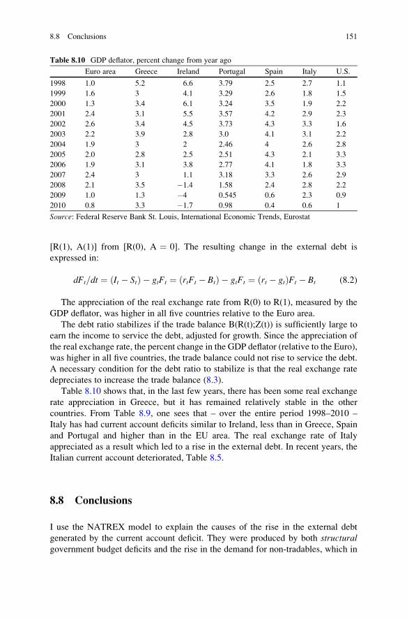
[R(1), A(1)] from [R(0), A ¼ 0]. The resulting change in the external debt is

expressed in:


The appreciation of the real exchange rate from R(0) to R(1), measured by the

GDP deflator, was higher in all five countries relative to the Euro area.

The debt ratio stabilizes if the trade balance B(R(t);Z(t)) is sufficiently large to

earn the income to service the debt, adjusted for growth. Since the appreciation of

the real exchange rate, the percent change in the GDP deflator (relative to the Euro),

was higher in all five countries, the trade balance could not rise to service the debt.

A necessary condition for the debt ratio to stabilize is that the real exchange rate

depreciates to increase the trade balance (8.3).

Table 8.10 shows that, in the last few years, there has been some real exchange

rate appreciation in Greece, but it has remained relatively stable in the other

countries. From Table 8.9, one sees that – over the entire period 1998–2010 –

Italy has had current account deficits similar to Ireland, less than in Greece, Spain

and Portugal and higher than in the EU area. The real exchange rate of Italy

appreciated as a result which led to a rise in the external debt. In recent years, the

Italian current account deteriorated, Table 8.5.

8.8 Conclusions

I use the NATREX model to explain the causes of the rise in the external debt

generated by the current account deficit. They were produced by both structuralgovernment budget deficits and the rise in the demand for non-tradables, which in

Table 8.10 GDP deflator, percent change from year ago

Euro area Greece Ireland Portugal Spain Italy U.S.

1998 1.0 5.2 6.6 3.79 2.5 2.7 1.1

1999 1.6 3 4.1 3.29 2.6 1.8 1.5

2000 1.3 3.4 6.1 3.24 3.5 1.9 2.2

2001 2.4 3.1 5.5 3.57 4.2 2.9 2.3

2002 2.6 3.4 4.5 3.73 4.3 3.3 1.6

2003 2.2 3.9 2.8 3.0 4.1 3.1 2.2

2004 1.9 3 2 2.46 4 2.6 2.8

2005 2.0 2.8 2.5 2.51 4.3 2.1 3.3

2006 1.9 3.1 3.8 2.77 4.1 1.8 3.3

2007 2.4 3 1.1 3.18 3.3 2.6 2.9

2008 2.1 3.5 �1.4 1.58 2.4 2.8 2.2

2009 1.0 1.3 �4 0.545 0.6 2.3 0.9

2010 0.8 3.3 �1.7 0.98 0.4 0.6 1

Source: Federal Reserve Bank St. Louis, International Economic Trends, Eurostat

8.8 Conclusions 151

turn appreciated the real exchange rate. This is the movement to the medium run

equilibrium R(1), A(1) in Fig. 8.2.

The SGP just focused upon the actual/realized budget deficit/GDP and assumed

that it was the factor that produced current account deficits. Hence, to avoid an

unsustainable debt, policy should be based upon realized budget deficits. This

approach is misleading for several reasons. First, the crucial variable in generating

crises is the external debt, not the internal debt. Second, one relevant variable for

the external debt in the NATREX model is the structural government budget

balance, the data in Table 8.1.

Third, realized budget deficits per se do not have a 1–1 correspondence withcurrent account deficits. The IMF analysis (IEO 2011, Fig. 8.4) showed that the

U.S. current account balance closely tracked the saving-investment balance of

households, while the fiscal balance showed little correlation. A similar situation

is true for the Euro area. Figure 8.4 is a scatter diagram relating the current account/

GDP to the realized government balance/GDP, for the entire Euro area. Surpluses

are positive and deficits are negative. There is not a positive relation between the

two.

There are several reasons for the absence of a 1–1 relation between realized

budget deficits and current account deficits. (a) The realized budget deficit, call it

Fig. 8.4 Euro area. Scatter diagram and regression line. Government budget balance/GDP and

current account/GDP (Source: ECB Statistical Data Warehouse)


GT* ¼ structural budget deficit + cyclical component. Hence GT* has a cyclical

component that is affected by the deviation of actual output from capacity output.

(b) The current account is also affected by the private sector difference between

investment and saving (I � Sp). (c) A high (I � Sp) raises income, raises the

current account deficit, raises tax receipts and lowers the realized government

budget deficit. In this case, the negative relation (I � Sp) and GT* leads to the

absence of a positive relation between GT* and the current account deficit.

The SGP rules must be viewed in the context of the NATREX model above. The

policy objective is generally to achieve a reduction in the external debt. No

sustained improvement in the external debt can occur unless the growth scenario

occurs. Growth and the trade balance function must increase. In the shorter run, the

real exchange rates of the five countries must depreciate relative to the Euro.

Bailouts and austerity policies will be ineffective in reducing the growth of the

debt unless the trade balance function B(R(t)) increases relative to the debt service

(r � g)F(t). The right hand side of Eq. 8.2 must decline.


In the NATREX model, output is at capacity Y(t) ¼ Y*(t), where Y(t) is actual

output and Y*(t) is capacity output. The trade balance function in the NATREX

model is B(R(t), Y*(t);Z(t)). The equality CA ¼ S � I is brought about by

variations in the real exchange rate, as shown Fig. 8.2. If the real exchange rate

R(t) ¼ R, ratio of domestic/foreign prices, is constant at R, then the variable of

adjustment must be Y(t). An austerity policy per se that raises social saving

(decrease government expenditures, raise taxes) will reduce GDP and induce a

decline in imports. Thereby B(t) rises because the decline in Y(t) below capacity

output reduces imports. But the austerity policy will neither induce growth of real

GDP, nor a sustainable rise in the trade balance function when GDP recovers.

It therefore will not be effective in reducing the growth of the debt in Eq. 8.2.

Austerity policies to be effective must produce the growth scenario.

The equilibrium value of the Euro per se has not necessarily been adversely

affected by the debt crises of the five countries. The actual value of the $US/Euroexchange rate is plotted in Fig. 8.5. The equilibrium value NATREX of the Euro-

$US depends upon the fundamentals, the two scenarios, in both the U.S. and Euro

area, not just in just one. To be sure there are large variations around the equilibrium

value due to speculative and cyclical factors. They average out to a mean of zero.

See Stein (2006, Chap. 5) for both a theoretical analysis and estimate of the

NATREX for Euro-$US in a two country setting.

Conclusions 153

References

Banco de Espagna. 2008. Annual report.

Bank for International Settlements, Eiglsperger, Martin, and Wim Haine, EU housing statistics

IFC Bulletin #31 Annex 1. 2009.

Bank of Greece. Annual report.

Cabral, R. 2010. VOX The PIGS’ external debt problem.

EEAG. 2011. EEAG report on the European economy. Munich: CESifo.

Fischer, Christoph. 2010. What can EMU countries’ sovereign bond spreads tell us about market

perceptions of default probabilities during the recent financial crisis? Niko D€otz Discussion

Paper Series 1: Economic Studies No. 11/2010.

International Monetary Fund, IEO. 2011. IMF performance in the run-up to the financial and

economic crisis.

International Monetary Fund. World Economic Outlook, Advanced economies: General govern-

ment structural balances, cyclically adjusted.

Irish Banking Crisis. 2010. Regulatory and financial stability policy 2003–2008, Report to

Minister of Finance by Governor of the Central Bank.

Moody’s US Municipal Bond Rating Scale 2002.

Plagnol, Valerie. 2010. European bond markets in financial crisis. Reuters: Ecowin.Stein, Jerome L. 2006. Stochastic optimal control, international finance and debt crises. Oxford:

Oxford University Press.

Williamson, John (ed.). 1994. Estimating equilibrium exchange rates. Washington, DC: Institute

for International Economics.

1.6

U.S. / Euro Foreign Exchange Rate (EXUSEU)Source: Board of Governors of the Federal Reserve System

Shaded areas indicate US recessions.

(U.S

.Dol

lars

to o

ne E

uro)


1.5

1.4

1.3

1.2

1.1

1.0

0.9

0.81998 2000 2002 2004 2006 2008 2010 2012

Fig. 8.5 Euro-$US exchange rate


Index

AActuarial literature, 7, 8, 97, 98, 101, 102

Agricultural crisis, 8, 13, 117, 119, 120, 129

American International Group (AIG), 2, 4, 7,

8, 23, 53–55, 59, 65–69, 89, 92, 94,

97–114

Anticipations of crisis, 13, 19–20

Apples in a basket model, 6, 36, 37, 50

Atlas capital funding, 34–35

Austerity policies, 133, 153

BBailout, 8, 24, 53, 59, 98, 99, 110–113, 129,

134, 135, 137, 139, 153

Bear Stearns, 2, 90, 91, 93, 112, 139

Bernanke, B., 14, 20, 92–94, 98, 112

Bielecki, T.R., 81

Black, F., 7, 39, 56, 106

Black-Scholes-Merton (BSM) options model,

6, 32, 38–40, 65

Blanchet-Scalliet, C., 47

Brownian motion (BM), 40, 58, 61, 62, 68,

69, 82, 83, 104, 105, 107, 108, 122

Bubble, 1, 4, 5, 7, 13–16, 20–22, 26, 32–34,

37, 41, 42, 46, 48, 50, 55, 75, 77, 78,

82, 84, 88, 91–94, 103, 114,

117–120, 143

CCapital gain, 4, 7, 8, 19–21, 32, 45–48, 50, 54,

55, 57–59, 65, 68, 69, 71, 77, 78, 80–84,

86–89, 102–108, 114, 119–122, 125,

127, 129, 130, 142

Capital requirements, 4, 7, 8, 13, 17–18, 26, 91,

92, 98, 100, 103, 104, 114, 130

CAPM model, 3, 6, 38–39

CDO. See Collateralized debt obligation

(CDO)

Citigroup, 2, 89, 91, 92

Collateralized debt obligation (CDO), 2, 6, 8,

34, 37–38, 41–45, 47, 50, 68, 69,

91–94, 98, 99, 106, 109, 111, 114

Cramer-Lundberg, 65–67, 70, 101, 102, 114

Credit default swap (CDS), 2, 22, 23, 32, 33,

44–47, 54, 55, 98, 138

Criterion function, 7, 8, 59–61, 67, 81, 98,

102, 104, 121

Current account to GDP ratio, 145

DDebt crises in Europe, 133–154

Debt equity ratio, 118–120, 125

Debtor-creditor by country, 140

Debt ratio, 5, 7–9, 14, 17, 18, 21, 32, 33,

46, 50, 53–55, 57–60, 62–64, 69,

71–73, 75, 76, 78, 80–87, 101, 103,

105, 106, 108, 109, 118–122, 124,

126–128, 133–135, 140–141, 145,

146, 149, 151

Debt service, 9, 20, 21, 77, 86, 87, 95,

121, 129, 133, 140, 153

Delinquency rate, 79, 117–120

Demyank, Y., 20, 77–79

Deregulation, 5, 13, 22–24, 26, 130

Derivatives market, 22, 23, 32, 35–38, 98

Derman, E., 7, 35, 43, 56, 71, 106

Disregarded warnings, 13–26

Dodd-Frank (D-F), 4, 9, 10, 22, 24

Dynamics net worth, 121–122

Dynamics real exchange rate and external

debt, 9, 143

J.L. Stein, Stochastic Optimal Control and the U.S. Financial Debt Crisis,DOI 10.1007/978-1-4614-3079-7, # Springer Science+Business Media New York 2012

155

EEarly warning signals (EWS), 4, 8, 32, 47,

53, 57, 75, 76, 80, 84, 86–88, 100,

103, 108–110, 114, 117, 119, 120,

127–129

EEAG, 136–138

Efficient Market Hypothesis (EMH), 5, 6,

17, 32, 38, 41–47, 50, 75

Euro, 135, 151, 153, 154

EWS. See Early warning signals (EWS)

Excess debt, 5, 7, 8, 13, 26, 53, 57, 63–65,

76, 80, 81, 84, 86–88, 95, 106, 109,

110, 119, 127–129

External debt to GDP, 137, 141–143

FFair game, 41

FDIC, 5, 23, 24, 26, 91, 118, 119

Fed, 3–6, 10, 13–26, 33, 35, 42, 88, 94,

113, 130

Federal reserve, 2, 4, 5, 14, 16, 21, 23, 24,

30, 59, 77, 78, 87, 110–113, 119,

135, 139, 141, 150, 151

Feller, W., 41, 66

Fidelity, 10, 34, 69, 140

Financial markets, 2–6, 9, 13, 14, 16, 17,

23, 25, 32, 33, 35, 43, 59, 70, 71,

75, 93, 97, 100, 111, 113, 114, 130,

133, 136, 137, 140

First theorem welfare economics, 5,

6, 16, 17

Fleming, W., 9, 10, 61, 81, 124

GGeneral government external debt, 141

Goldman-Sachs, 2, 91, 99

Gorton model, 69, 99, 110, 114

Government net debt, 134, 135, 141

Government structural balance, 134, 135

Granger causality, 119, 120

Greece, 134–138, 140–142, 149–151

Greenspan, A., 4–6, 10, 13–18, 20,

22, 23, 35, 42, 50, 80, 88, 92,

94, 113

Growth scenario, 146–149, 153

HHouse price index, 16, 43–48, 86, 88, 104

Housing sector, 13, 54, 55, 76, 136, 137

IIMF, 3–5, 13–26, 33, 53, 88, 134, 135, 152

Independent evaluation office IMF, 3, 24

Insurance, 2, 4, 7, 8, 23, 24, 35, 54, 55, 59, 65–69,

98, 100–104, 106, 109–111, 129, 138

Interest rate spreads, 138, 139

International monetary fund, 24–25

Ireland, 91, 134–138, 140–142, 149–151

Issing, O., 15, 16

Italy, 134, 135, 140–142, 149–151

JJackson Hole Consensus, 5, 15–17, 20, 21, 26

Juselius, M., 76, 95

KKim, M., 76, 95

LLehman Brothers, 2, 93, 99, 111, 136, 138, 139

Leverage, 2–8, 13–15, 17–19, 21, 23–26,

32–35, 42, 53, 54, 69, 76, 80, 82,

88–95, 99, 101–106, 109

LIBOR. See London Interbank Offered Rate

(LIBOR)

Linkages, 24, 34, 76, 89–95, 140

London Interbank Offered Rate (LIBOR),

100, 113

MMark to market (M-t-M), 44, 90, 92, 102

Martingale, 41–45

Mean Variance, 60, 61, 105, 124, 126–127

Merrill-Lynch, 2, 90–92

Model I, 57, 65, 71–73, 80–84, 88

Model II, 57, 61, 65, 71–73, 80, 81, 83–85, 107

Modeling, 7, 43, 57–59, 68, 69, 104, 106, 107

Model uncertainty, 58, 64, 106–108

Moody’s, 36, 37, 92, 139

Mortgage market, 7, 25, 30, 32, 36, 75–79,

93, 136

NNAP. See No Arbitrage Principle (NAP)

Natural real exchange rate (NATREX),

9, 134, 136, 143–153

No Arbitrage Principle (NAP), 32, 38–47

156 Index

OOffice thrift supervision (OTS), 100, 114

OIS. See Overnight index spread rate (OIS)

Optimal control, 9, 57, 60, 61

Optima liabilities large insurer, 100, 102–103

Optimum debt ratio, 60, 62–64, 80, 83, 84

Ornstein-Uhlenbeck, 57, 72, 122, 123

OTS. See Office thrift supervision (OTS)

Overnight index spread rate (OIS), 100, 113

PPhilosophy stochastic optimal control, 53–73

Platen-Rebolledo, 81

Pliska, S., 81

Populist scenario, 146–149

Portugal, 134–136, 138, 140–142, 149–151

PRICEINC, 20, 21, 86, 87

Prince, Charles, 22, 89, 100

Properly anticipated prices, 41–43

QQuants, 3, 4, 6, 8, 17, 24, 29–50, 56, 58,

75, 78, 81, 87, 89

RRating agencies, 4, 14, 32, 34–38, 43,

44, 92, 94

Rentprice, 85–87

Rescue, 4, 15, 111–113, 129, 139

Residential property prices EU, 142

Rishel, R., 9, 10, 56, 58, 61

Risk aversion, 7, 48, 60, 67

Ruin analysis, 66–67

SSamuelson, Paul, 41, 44

Shadow banking system, 8, 53, 54, 70, 75,

76, 89–95, 120

S&L crisis, 8, 13, 117, 129, 130

Slices of bread in loaf model, 50

SOC. See Stochastic optimal control (SOC)

Solution of stochastic optimal control, 61–63

Spain, 91, 134–138, 140–142, 149–151

Stochastic differential equations, 8, 57, 58,

61, 68, 69, 71, 80, 81, 98, 104, 105,

121, 122

Stochastic optimal control (SOC), 4, 7–10,

17, 18, 26, 32, 53–73, 75–95, 97, 98,

100, 102–103, 110, 114, 117,

119–122, 129, 134

Stochastic processes, 7, 47, 49, 80, 81, 103,

124, 127

TTED, 100

Tranches, 2, 6, 32, 36–38, 41–44, 50, 69, 91,

92, 99, 114

UUncertainty, 2, 57–59, 64, 80–82, 93,

106–108, 121–123

US municipal rating, 139

Utility functions, 6, 17, 38, 48, 59, 60

VVan Hemert, O., 20, 77–79

Volchan, S., 65, 101

Index 157

stochastic optimal control and the u.s financial debt crisis

Economy & Finance

general use

springer science

exclusive use

stochastic variables

financial debt crisis

mortgage debt crisis

respective copyright

acidfree paper springer