stochastic optimal control in mathematical finance
TRANSCRIPT
Jan Kallsen
Stochastic Optimal Control inMathematical Finance
CAU zu Kiel, WS 15/16, as of April 21, 2016
Contents
0 Motivation 4
I Discrete time 7
1 Recap of stochastic processes 81.1 Processes, stopping times, martingales . . . . . . . . . . . . . . . . . . . . 81.2 Stochastic integration . . . . . . . . . . . . . . . . . . . . . . . . . . . . . 161.3 Conditional jump distribution . . . . . . . . . . . . . . . . . . . . . . . . . 221.4 Essential supremum . . . . . . . . . . . . . . . . . . . . . . . . . . . . . . 25
2 Dynamic Programming 27
3 Optimal Stopping 34
4 Markovian situation 40
5 Stochastic Maximum Principle 45
II Continuous time 60
6 Recap of stochastic processes 626.1 Continuous semimartingales . . . . . . . . . . . . . . . . . . . . . . . . . 62
6.1.1 Processes, stopping times, martingales . . . . . . . . . . . . . . . . 626.1.2 Brownian motion . . . . . . . . . . . . . . . . . . . . . . . . . . . 686.1.3 Quadratic variation . . . . . . . . . . . . . . . . . . . . . . . . . . 696.1.4 Square-integrable martingales . . . . . . . . . . . . . . . . . . . . 726.1.5 Stopping times . . . . . . . . . . . . . . . . . . . . . . . . . . . . 73
6.2 Stochastic integral . . . . . . . . . . . . . . . . . . . . . . . . . . . . . . . 746.2.1 Differential notation . . . . . . . . . . . . . . . . . . . . . . . . . 806.2.2 Ito processes . . . . . . . . . . . . . . . . . . . . . . . . . . . . . 806.2.3 Ito diffusions . . . . . . . . . . . . . . . . . . . . . . . . . . . . . 816.2.4 Doléans exponential . . . . . . . . . . . . . . . . . . . . . . . . . 836.2.5 Martingale representation . . . . . . . . . . . . . . . . . . . . . . 856.2.6 Change of measure . . . . . . . . . . . . . . . . . . . . . . . . . . 85
2

CONTENTS 3
7 Dynamic programming 87
8 Optimal stopping 90
9 Markovian situation 959.1 Stochastic control . . . . . . . . . . . . . . . . . . . . . . . . . . . . . . . 959.2 Optimal Stopping . . . . . . . . . . . . . . . . . . . . . . . . . . . . . . . 98
10 Stochastic maximum principle 102
Bibliography 108
Chapter 0
Motivation
In Mathematical Finance one often faces optimization problems of various kinds, in par-ticular when it comes to choosing trading strategies with in some sense maximal utility orminimal risk. The choice of an optimal exercise time of an American option belongs to thiscategory as well. Such problems can be tackled with different methods. We distinguish twomain approaches, which are discussed both is discrete and in continuous time. As a motiva-tion we first consider the simple situation of maximizing a deterministic function of one orseveral variables.
Example 0.1 1. (Direct approach) Suppose that the goal is to maximize a function
(x, α) 7→T∑t=1
f(t, xt−1, αt) + g(xT )
over all x = (x1, . . . , xT ) ∈ (Rd)T , α = (α1, . . . , αT ) ∈ AT such that
∆xt := xt − xt−1 = δ(xt−1, αt), t = 1, . . . , T
for some given function δ : Rd × Rm → Rd. The initial value x0 ∈ Rd, the statespace of controls A ⊂ Rm and the objective functions f : 1, . . . , T×Rd×A→ R,g : Rd → R are supposed to be given. The approach in Chapters 2 and 7 below corre-sponds to finding the maximum directly, without relying on smoothness or convexityof the functions f, g, δ or on topological properties of A. Rather, the idea is to reducethe problem to a sequence of simpler optimizations in just one A-valued variable αt.
2. (Lagrange multiplier approach) Since the problem above concerns constrained opti-mization, Lagrange multiplier techniques may make sense. To this end, define theLagrange function
L(x, α, y) :=T∑t=1
f(t, xt−1, αt) + g(xT )−T∑t=1
yt(∆xt − δ(xt−1, αt))
on (Rd)T×AT×(Rd)T . The usual first-order conditions lead us to look for a candidatex? ∈ (Rd)T , α? ∈ AT , y? ∈ (Rd)T satisfying
(a) ∆x?t = δ(x?t−1, α?t ) for t = 1, . . . , T , where we set x?0 := x0,
4

5
(b) y?T = ∇g(x?T ),
(c) ∆y?t = −∇xH(t, x?t−1, α?t ) for t = 1, . . . , T, where we set H(t, ξ, a) :=
f(t, ξ, a) + y?t δ(ξ, a) and ∇xH denotes the gradient of H viewed as a functionof its second argument,
(d) α?t maximizes a 7→ H(t, x?t−1, a) on A for t = 1, . . . , T .
Provided that some convexity conditions hold, a–d) are in fact sufficient for optimalityof α?:
Lemma 0.2 Suppose that the set A is convex, ξ 7→ g(ξ), (ξ, a) 7→ H(t, ξ, a), t =1, . . . , T are concave and ξ 7→ g(ξ), ξ 7→ H(t, ξ, a), t = 1, . . . , T , a ∈ A aredifferentiable. If Conditions a–d) hold, then (x?, α?) is optimal for the problem inExample 0.1(1).
Proof. For any competitor (x, α) satisfying the constraints set h(t, ξ) :=supa∈AH(t, ξ, a). Condition d) yields h(t, x?t−1) = H(t, x?t−1, α
?t ) for t = 1, . . . , T .
We have
T∑t=1
f(t, xt−1, αt) + g(xT )−T∑t=1
f(t, x?t−1, α?t )− g(x?T )
=T∑t=1
(H(t, xt−1, αt)−H(t, x?t−1, α
?t )− y?t (∆xt −∆x?t )
)+ g(xT )− g(x?T )
≤T∑t=1
((H(t, xt−1, αt)− h(t, xt−1)) +
(h(t, xt−1)− h(t, x?t−1)
)− y?t (∆xt −∆x?t )
)+∇g(x?T )(xT − x?T )
≤T∑t=1
(∇xh(t, x?t−1)(xt−1 − x?t−1)− y?t (∆xt −∆x?t )
)+∇g(x?T )(xT − x?T ) (0.1)
=T∑t=1
(−∆y?t (xt−1 − x?t−1)− y?t (∆xt −∆x?t )
)+ y?T (xT − x?T ) (0.2)
= y?0(x0 − x?0)
= 0
where existence of ∇xh(t, x?t−1), inequality (0.1) as well as equation (0.2) followfrom Lemma 0.3 below and the concavity of g.
Under some more convexity (e.g. if δ is affine and f(t, ·, ·) is concave for t =1, . . . , T ), the Lagrange multiplier solves some dual minimisation problem. This hap-pens e.g. in the stochastic examples 5.3–5.8 in Chapter 5.
6 CHAPTER 0. MOTIVATION
The following lemma is a version of the envelope theorem which makes a statement onthe derivative of the maximum of a parametrised function.
Lemma 0.3 Let A be a convex set, f : Rd × A → R ∪ −∞ a concave function, andf(x) := supa∈A f(x, a), x ∈ Rd. Then f is concave. Suppose in addition that, for some fixedx? ∈ Rd, the optimizer a? := argmaxa∈Af(x?, a) exists and x 7→ f(x, a?) is differentiablein x?. Then f is differentiable in x? with derivative
Dif(x?) = Dif(x?, a?), i = 1, . . . , d. (0.3)
Proof. One easily verifies that f is concave. For h ∈ Rd we have
f(x? + yh) ≥ f(x? + yh, a?)
= f(x?, a?) + y
d∑i=1
Dif(x?, a?)hi + o(y)
as y ∈ R tends to 0. In view of [HUL13, Proposition I.1.1.4], concavity of f implies thatwe actually have
f(x? + yh) ≤ f(x?, a?) + yd∑i=1
Dif(x?, a?)hi
and hence differentiability of f in x? with derivative (0.3).
In the remainder of this course we consider optimization in a dynamic stochastic setup.Green parts in these notes are skipped either because they are assumed to be known (Chap-ters 1 and 6) or for lack of time. Comments are welcome, in particular if they concern errorsin this text.
Part I
Discrete time
7

Chapter 1
Recap of stochastic processes
The theory of stochastic processes deals with random functions of time as e.g. asset prices,interest rates, or trading strategies. As is true for Mathematical Finance as well, it canbe developped in both discrete and continuous time. Actual calculations are sometimeseasier and more transparent in continuous-time models, but the theory typically requiresless background in discrete time.
1.1 Processes, stopping times, martingales
The natural starting point in probability theory is a probability space (Ω,F , P ). The moreor less abstract sample space Ω stands for the possible outcomes of the random experiment.It could e.g. contain all conceivable sample paths of a stock price process. The probabilitymeasure P assigns probabilities to subsets of outcomes. For measure theoretic reasons it istypically impossible to assign probabilities to all subsets of Ω in a consistent manner. Asa way out one specifies a σ-field F , i.e. a collection of subsets of Ω which is closed undercountable set operations as e.g. ∩,∪, \, C . The probability P (F ) is defined only for eventsF ∈ F .
Random variables X are functions of the outcome ω ∈ Ω. Typically its values X(ω)are numbers but they may also be vectors or even functions, in which case X is a randomvector resp. process. We denote by E(X), Var(X) the expected value and variance of areal-valued random variable. Accordingly, E(X), Cov(X) denote the expectation vectorand covariance matrix of a random vector X .
For static random experiments one needs to consider only two states of information.Before the experiment nothing precise is known about the outcome, only probabilities andexpected values can be assigned. After the experiment the outcome is completely deter-mined. In dynamic random experiments as e.g. stock markets the situation is more involved.During the time interval of observation, some random events (e.g. yesterday’s stock returns)have already happened and can be considered as deterministic whereas others (e.g. tomor-rows’ stock returns) still belong to the unknown future. As time passes, more and moreinformation is accumulated.
This increasing knowledge is expressed mathematically in terms of a filtration F =(Ft)t≥0, i.e. an increasing sequence of sub-σ-fields of F . The collection of events Ft
stands for the observable information up to time t. The statement F ∈ Ft means that the
8
1.1. PROCESSES, STOPPING TIMES, MARTINGALES 9
random event F (e.g. F = stock return positive at time t−1) is no longer random at time t.We know for sure whether it is true or not. If our observable information is e.g. given by theevolution of the stock price, then Ft contains all events that can be expressed in terms of thestock price up to time t. The quadrupel (Ω,F ,F, P ) is called filtered probability space.We consider it to be fixed during most of the following. Often one assumes F0 = ∅,Ω,i.e. F0 is the trivial σ-field corresponding to no prior information.
As time passes, not only the observable information but also probabilities and expec-tations of future events change. E.g. our conception of the terminal stock price evolvesgradually from vague ideas to perfect knowledge. This is modelled mathematically in termsof conditional expectations. The conditional expectation E(X|Ft) of a random variable Xis its expected value given the information up to time t. As such, it is not a number but itselfa random variable which may depend on the randomness up to time t, e.g. on the stock priceup to t in the above example. Mathematically speaking, Y = E(X|Ft) is Ft-measurable,which means that Y ∈ B := ω ∈ Ω : Y (ω) ∈ B ∈ Ft for any reasonable (i.e. Borel)setB. Accordingly, the conditional probability P (F |Ft) denotes the probability of an eventF ∈ F given the information up to time t. As is true for conditional expectation, it is not anumber but an Ft-measurable random variable.
Formally, the conditional expectationE(X|Ft) is defined as the unique Ft-measurablerandom variable Y such that E(XZ) = E(Y Z) for any bounded, Ft-measurable randomvariable Z. It can also be interpreted as the best prediction of X given Ft. Indeed, ifE(X2) < ∞, then E(X|Ft) minimizes the mean squared difference E((X − Z)2) amongall Ft-measurable random variables Z. Strictly speaking, E(X|Ft) is unique only up to aset of probability 0, i.e. any two versions Y, Y satisfy P (Y 6= Y ) = 0. In this notes we donot make such fine distinctions. Equalities, inequalities etc. are always meant to hold onlyalmost surely, i.e. up to a set of probability 0.
A few rules on conditional expectations are used over and over again. E.g. we have
E(X|Ft) = E(X) (1.1)
if Ft = ∅,Ω is the trivial σ-field representing no information on random events. Moregenerally, (1.1) holds if X and Ft are stochastically independent, i.e. if
P (X ∈ B ∩ F ) = P (X ∈ B)P (F )
for any reasonable (i.e. Borel) set B and any F ∈ Ft. On the other hand we haveE(X|Ft) = X and more generally
E(XY |Ft) = XE(Y |Ft)
if X is Ft-measurable, i.e. known at time t. The law of iterated expectations tells us that
E(E(X|Ft)
∣∣Fs
)= E(X|Fs)
for s ≤ t. Almost as a corollary we have
E(E(X|Ft)
)= E(X).
Finally, the conditional expectation shares many properties of the expectation, e.g, it is linearand monotone in X and it satisfies monotone and dominated convergence, Fatou’s lemma,Jensen’s inequality etc.
10 CHAPTER 1. RECAP OF STOCHASTIC PROCESSES
Recall that the probability of a set can be expressed as expectation of an indicator func-tion via P (F ) = E(1F ). This suggests to use the relation
P (F |Ft) := E(1F |Ft) (1.2)
to define conditional probabilities in terms of conditional expectation. Of course, we wouldlike P (F |Ft) to be a probability measure when it is considered as a function of F . Thisproperty, however, is not as evident as it seems because of the null sets involved in the defi-nition of conditional expectation. We do not worry about technical details here and assumeinstead that we are given a regular conditional probability, i.e. a version of P (F |Ft)(ω)which, for any fixed ω, is a probability measure when viewed as a function of F . Such aregular version exists in all instances where it is used in this notes.
In line with (1.2) we denote by
PX|Ft(B) := P (X ∈ B|Ft) := E(1B(X)|Ft)
the conditional law of X given Ft. A useful rule states that
E(f(X, Y )|Ft) =
∫f(x, Y )PX|Ft(dx) (1.3)
for real-valued functions f and Ft-measurable random variables Y . If X is stochasticallyindependent of Ft, we have PX|Ft = PX , i.e. the conditional law of X coincides with thelaw of X . In this case, (1.3) turns into
E(f(X, Y )|Ft) =
∫f(x, Y )PX(dx) (1.4)
for Ft-measurable random variables Y .A stochastic process X = (X(t))t≥0 is a collection of random variables X(t), indexed
by time t. In this section, the time set is assumed to be N = 0, 1, 2, . . . , afterwardswe consider continuous time R+ = [0,∞). As noted earlier, a stochastic process X =(X(t))t≥0 can be interpreted as a random function of time. Indeed, X(ω, t) is a functionof t (or sequence in the current discrete case) for fixed ω. Sometimes, it is also convenientto interpret a process X as a real-valued function on the product space Ω × N or Ω × R+,respectively. In the discrete time case we use the notation
∆X(t) := X(t)−X(t− 1).
Moreover we denote by X− = (X−(t))t≥0 the process
X−(t) :=
X(t− 1) for t ≥ 1,X(0) for t = 0.
(1.5)
We will only consider processes which are consistent with the information structure, i.e.X(t) is supposed to be observable at time t. Mathematically speaking, we assume X(t) tobe Ft-measurable for any t. Such processes X are called adapted (to the filtration F).
There is in fact a minimal filtration F such that X is F-adapted. Formally, this filtrationis given by
Ft = σ(X(s) : s ≤ t), (1.6)
1.1. PROCESSES, STOPPING TIMES, MARTINGALES 11
i.e. Ft is the smallest σ-field such that all X(s), s ≤ t are Ft-measurable. Intuitively, thismeans that the only information on random events is coming from observing the process X .One calls F the filtration generated by X .
For some processes one actually needs a stronger notion of measurability than adapted-ness, namely predictability. A stochastic process X is called predictable if X(t) is knownalready one period in advance, i.e. X(t) is Ft−1-measurable. The use of this notion willbecome clearer in Section 1.2.
Example 1.1 (Random walk and geometric random walk) We call an adapted process Xrandom walk (relative to F) if the increments ∆X(t), t ≥ 1 are identically distributedand independent of Ft−1. We obtain such a process if ∆X(t), t ≥ 1 are independent andidentically distributed (i.i.d.) random variables and if the filtration F is generated by X .
Similarly, we call a positive adapted process X geometric random walk (relative to F)if the relative increments
∆X(t)
X(t− 1)=
X(t)
X(t− 1)− 1 (1.7)
are identically distributed and independent of Ft−1 for t ≥ 1. A process X is a geometricrandom walk if and only if log(X) is a random walk or, equivalently,
X(t) = exp(Y (t))
for some random walk Y . Indeed, the random variables in (1.7) are identically distributedand independent of Ft−1 if and only this holds for
∆(logX(t)) = log(X(t))− log(X(t− 1)) = log
(∆X(t)
X(t− 1)+ 1
), t ≥ 1.
Random walks and geometric random walks represent processes of constant growth inan additive or multiplicative sense, respectively. Simple asset price models are often ofgeometric random walk type.
A stopping time τ is a random variable whose values are times, i.e. are in N∪∞ in thediscrete case. Additionally one requires that τ is consistent with the information structureF. More precisely, one assumes that τ = t ∈ Ft (or equivalently τ ≤ t ∈ Ft) for anyt. Intuitively, this means that the decision to say “stop!” right now can only be based on ourcurrent information. As an example consider the first time τ when the observed stock pricehits the level 100. Even though this time is random and not known in advance, we obviouslyknow τ in the instant it occurs. The situation is different if we define τ to be the instantone period before the stock hits 100. Since we cannot look into the future, we only know τone period after it has happened. Consequently, this random variable is not a stopping time.Stopping times occur naturally in finance e.g. in the context of American options but theyalso play an important technical role in stochastic calculus.
As indicated above, the time when some adapted process first hits a given set is a stop-ping time:
Lemma 1.2 Let X be some adapted process and B a Borel set. Then
τ := inft ≥ 0 : X(t) ∈ B
is a stopping time.
12 CHAPTER 1. RECAP OF STOCHASTIC PROCESSES
Proof. By adaptedness, we have X(s) ∈ B ∈ Fs ⊂ Ft, s ≤ t and hence
τ ≤ t =t⋃
s=0
X(s) ∈ B ∈ Ft.
Occasionally, it turns out to be important to “freeze” a process at a stopping time. Forany adapted process X at any stopping time τ , the process stopped at τ is defined as
Xτ (t) := X(τ ∧ t),
where we use the notation a ∧ b := min(a, b) as usual. The stopped process Xτ remainsconstant on the level X(τ) after time τ . It is easy to see that it is adapted as well.
The concept of martingales is central to stochastic calculus and finance. A martingale(resp. submartingale, supermartingale) is an adapted process X that is integrable (in thesense that E(|X(t)|) <∞ for any t) and satisfies
E(X(t)|Fs) = X(s) (resp. ≥ X(s),≤ X(s)) (1.8)
for s ≤ t. If X is a martingale, then the best prediction for future values is the present level.If e.g. the price process of an asset is a martingale, then it is neither going up nor downon average. In that sense, it correponds to a fair game. By contrast, submartingales (resp.supermartingales) may increase (resp. decrease) on average. They correspond to favourable(resp. unfavourable) games.
The concept of a martingale is “global” in the sense that (1.8) must be satisfied for anys ≤ t. If we restrict attention to the case s = t − 1, we obtain the slightly more general“local” counterpart. A local martingale (resp. submartingale, supermartingale) is anadapted process X which satisfies E(|X(0)|) <∞, E(|X(t)||Ft−1) <∞ and
E(X(t)|Ft−1) = X(t− 1) (resp. ≥ X(t− 1),≤ X(t− 1)) (1.9)
for any t = 1, 2, . . . In discrete time the difference between martingales and local martin-gales is minor:
Lemma 1.3 Any integrable local martingale (in the sense that E(|X(t)|) <∞ for any t) isa martingale. An analogous statement holds for sub- and supermartingales.
Proof. This follows by induction from the law of iterated expectations.
Corresponding statements hold for sub-/supermartingales. Integrability in Lemma 1.3holds e.g. if X is nonnegative.
The above classes of processes are stable under stopping in the sense of the followinglemma, which has a natural economic interpretation: you cannot turn a fair game into e.g. astrictly favourable one by stopping to play at some reasonable time.
Lemma 1.4 Let τ denote a stopping time. If X is a martingale (resp. sub-/super-martingale), so is Xτ . A corresponding statement holds for local martingales and localsub-/supermartingales.

1.1. PROCESSES, STOPPING TIMES, MARTINGALES 13
Proof. We start by verifying the integrability conditions. For martingales (resp. sub-supermartingales) E(|X(t)|) < ∞ implies E(|Xτ (t)|) ≤ E(
∑ts=0 |X(s)|) < ∞. For
local martingales (resp. local sub-/supermartingales) E(|X(t)||Ft−1) <∞ yields
E(|Xτ (t)||Ft−1) ≤t∑
s=0
E(|X(s)||Ft−1)
=t∑
s=0
|X(s)|+ E(|X(t)||Ft−1) <∞.
In order to verify (1.9), observe that τ ≥ t = τ ≤ t− 1C ∈ Ft−1 implies
E(Xτ (t)1τ≥t|Ft−1) = E(X(t)1τ≥t|Ft−1)
= E(X(t)|Ft−1)1τ≥t
= X(t− 1)1τ≥t
= Xτ (t− 1)1τ≥t
(resp. ≥,≤ in the sub-/supermartingale case). For s < t we have τ = s ∈ Fs ⊂ Ft−1
and hence
E(Xτ (t)1τ=s|Ft−1) = E(X(s)1τ=s|Ft−1)
= X(s)1τ=s
= Xτ (t− 1)1τ=s.
Together we obtain
E(Xτ (t)|Ft−1) =t−1∑s=0
E(Xτ (t)1τ=s|Ft−1) + E(X(t)1τ≥t|Ft−1)
=t−1∑s=0
Xτ (t− 1)1τ=s +Xτ (t− 1)1τ≥t = Xτ (t− 1)
(resp. ≥,≤).
For later use, we note that a supermartingale with constant expectation is actually amartingale.
Lemma 1.5 If X is a supermatingale and T ≥ 0 with E(X(T )) = E(X(0)), then (1.8)holds with equality for any s ≤ t ≤ T .
Proof. The supermartingale property means that E((X(t) − X(s))1A) ≤ 0 for any s ≤ tand any A ∈ Fs. Since
0 = E(X(T ))− E(X(0))
= E(X(T )−X(t)) + E((X(t)−X(s))1A) + E((X(t)−X(s))1Ac)
+ E(X(s)−X(0))
≤ 0

14 CHAPTER 1. RECAP OF STOCHASTIC PROCESSES
for any s ≤ t ≤ T and any event A ∈ Fs, the four nonpositive summands must actually be0. This yields E((X(t)−X(s))1A) = 0 and hence the assertion.
The following technical result is used in Chapter 3.
Lemma 1.6 Let X be a supermartingale, Y a martingale, t ≤ T , and A ∈ Ft with X(t) =Y (t) on A and X(T ) ≥ Y (T ). Then X(s) = Y (s) on A for t ≤ s ≤ T . The statementremains to hold if we only requireXT−X t, Y T−Y t instead ofX, Y to be a supermartingaleresp. martingale.
Proof. FromX(s)− Y (s) ≥ E(X(T )− Y (T )|Fs) ≥ 0
andE((X(s)− Y (s))1A) ≤ E((X(t)− Y (t))1A) = 0
it follows that (X(t)− Y (t))1A = 0.
One easily verifies that an integrable random walk X is a martingale if (and only if) theincrements ∆X(t) have expectation 0. An analogous result holds for integrable geomet-ric random walks whose relative increments ∆X(t)/X(t− 1) have vanishing mean. Forthe martingale property to hold, one actually does not need the increments resp. relativeincrements of X to be identically distributed.
If ξ denotes an integrable random variable, then it naturally induces a martingale X ,namely
X(t) = E(ξ|Ft).
X is called the martingale generated by ξ. If the time horizon is finite, i.e. we considerthe time set 0, 1, . . . , T − 1, T rather then N, then any martingale is generated by somerandom variable, namely by X(T ). This ceases to be true for infinite time horizon. E.g.random walks are not generated by a single random variable unless they are constant.
Example 1.7 (Density process) A probability measure Q on (Ω,F ) is called equivalentto P (written Q ∼ P ) if the events of probability 0 are the same under P and Q. Bythe Radon-Nikodym theorem, Q has a P -density and vice versa, i.e. there are some uniquerandom variables dQ
dP, dPdQ
such that
Q(F ) = EP
(1FdQ
dP
), P (F ) = EQ
(1FdP
dQ
)for any set F ∈ F , where EP , EQ denote expectation under P and Q, respectively. P,Qare in fact equivalent if and only if such mutual densities exist, in which case we havedPdQ
= 1/dQdP
.The martingale Z generated by dQ
dPis called density process of Q, i.e. we have
Z(t) = EP
(dQ
dP
∣∣∣∣Ft
).

1.1. PROCESSES, STOPPING TIMES, MARTINGALES 15
One easily verifies that Z(t) coincides with the density of the restricted measures Q|Ft
relative to P |Ft, i.e. Z(t) is Ft-measurable and
Q(F ) = EP (1FZ(t))
holds for any event F ∈ Ft. Note further that Z and the density process Y of P relative toQ are reciprocal to each other because
Z(t) =dQ|Ft
dP |Ft
= 1/dP |Ft
dQ|Ft
= 1/Y (t).
The density process Z can be used to compute conditional expectations relative to Q.Indeed, the generalized Bayes’ rule
EQ(ξ|Ft) =EP (ξ dQ
dP|Ft)
Z(t)
holds for sufficiently integrable random variables ξ because
EQ(ξζ) = EP
(ξζdQ
dP
)= EP
(EP
(ξζdQ
dP
∣∣∣∣Ft
))= EP
(EP
(ξζ dQ
dP
Z(t)
∣∣∣∣Ft
)Z(t)
)
= EQ
(EP
(ξζ dQ
dP
Z(t)
∣∣∣∣Ft
))
= EQ
(EP (ξ dQ
dP|Ft)
Z(t)ζ
)for any bounded Ft-measurable ζ . Similarly, one shows
EQ(ξ|Fs) =EP (ξZ(t)|Fs)
Z(s)(1.10)
for s ≤ t and Ft-measurable random variables ξ.
Martingales are expected to stay on the current level on average. More general processesmay show an increasing, decreasing or possibly variable trend. This fact is expressed for-mally by a variant of Doob’s decomposition. The idea is to decompose the increment ∆X(t)of an arbitrary process into a predictable trend component ∆AX(t) and a random deviation∆MX(t) from this short time prediction.
Lemma 1.8 (canonical decomposition) Any integrable adapted process X (i.e. withE(|X(t)|) <∞ for any t) can be uniquely decomposed as
X = X(0) +MX + AX
with some martingale MX and some predictable process AX satisfying MX(0) = AX(0) =0. We call AX the compensator of X .
16 CHAPTER 1. RECAP OF STOCHASTIC PROCESSES
Proof. Define AX(t) =∑t
s=1 ∆AX(s) by ∆AX(s) := E(∆X(s)|Fs−1) and MX := X −X(0)−AX . Predictability of AX is obvious. The integrability of X implies that of AX andthus of MX . The latter is a martingale because
E(MX(t)|Ft−1) = MX(t− 1) + E(∆X(t)−∆AX(t)|Ft−1)
= MX(t− 1) + E(∆X(t)|Ft−1)− E(E(∆X(t)|Ft−1)|Ft−1)
= MX(t− 1).
Conversely, for any decomposition as in Lemma 1.8 we have
E(∆X(t)|Ft−1) = E(∆MX(t)|Ft−1) + E(∆AX(t)|Ft−1) = ∆AX(t),
which means that it coincides with the decomposition in the first part of the proof.
Note that uniqueness of the decomposition still holds if we only require MX to be alocal martingale. In this relaxed sense, it suffices to assume E(|X(t)||Ft−1) <∞ for any tin order to define the compensator AX .
IfX is a submartingale (resp. supermartingale), thenAX is increasing (resp. decreasing).This is the case commonly referred to as Doob’s decomposition. E.g. the compensator ofan integrable random walk X equals
AX(t) =t∑
s=1
E(∆X(s)|Fs−1) = tE(∆X(1)).
1.2 Stochastic integrationGains from trade in dynamic portfolios can be expressed in terms of stochastic integrals,which are nothing else than sums in discrete time.
Definition 1.9 LetX be an adapted and ϕ a predictable (or at least also an adapted) process.The stochastic integral of ϕ relative to X is the adapted process ϕ • X defined as
ϕ • X(t) :=t∑
s=1
ϕ(s)∆X(s).
If both ϕ = (ϕ1, . . . , ϕd) and X = (X1, . . . , Xd) are vector-valued processes, we defineϕ • X to be the real-valued process given by
ϕ • X(t) :=t∑
s=1
d∑i=1
ϕi(s)∆Xi(s). (1.11)
In order to motivate this definition, let us interpret X(t) as the price of a stock at time t.We invest in this stock using the trading strategy ϕ, i.e. ϕ(t) denotes the number of shareswe own at time t. Due to the price move from X(t − 1) to X(t) our wealth changes byϕ(t)(X(t)−X(t− 1)) = ϕ(t)∆X(t) in the period between t− 1 and t. Consequently, the

1.2. STOCHASTIC INTEGRATION 17
integral ϕ • X(t) stands for the cumulative gains from trade up to time t. If we invest in aportfolio of several stocks, both the trading strategy ϕ and the price process X are vectorvalued. ϕi(t) now stands for the number of shares of stock i and Xi(t) for its price. In orderto compute the total gains of the portfolio, we must sum up the gains ϕi(t)∆Xi(t) in eachsingle stock, which leads to (1.11).
For the above reasoning to make sense, one must be careful about the order in whichthings happen at time t. If ϕ(t)(X(t)−X(t− 1)) is meant to stand for the gains at time t,we obviously have to buy the portfolio ϕ(t) before prices change from X(t − 1) to X(t).Put differently, we must choose ϕ(t) already at the end of period t− 1, right after the stockprice has attained the value X(t − 1). This choice can only be based on information upto time t − 1 and in particular not on X(t), which is as yet unknown. This motivates whyone typically requires trading strategies to be predictable rather than adapted. The purelymathematical definition of ϕ • X , however, makes sense regardless of any measurabilityassumption.
The covariation process [X, Y ] of adapted processes X, Y is defined as
[X, Y ](t) :=t∑
s=1
∆X(s)∆Y (s). (1.12)
Its compensator
〈X, Y 〉(t) =t∑
s=1
E(∆X(s)∆Y (s) |Fs−1)
is called predictable covariation process if it exists. In the special case X = Y onerefers to the quadratic variation resp. predictable quadratic variation of X . If X, Yare martingales, their predictable covariation can be viewed as a dynamic analogue of thecovariance of two random variables.
We are now ready to state a few properties of stochastic integration:
Lemma 1.10 For adapted processes X, Y and predictable processes ϕ, ψ we have:
1. ϕ • X is linear in ϕ and X .
2. [X, Y ] and 〈X, Y 〉 are symmetric and linear in X and Y .
3. ψ • (ϕ • X) = (ψϕ) • X
4. [ϕ • X, Y ] = ϕ • [X, Y ]
5. 〈ϕ • X, Y 〉 = ϕ • 〈X, Y 〉 whenever the predictable covariations are defined.
6. (integration by parts)
XY = X(0)Y (0) +X− • Y + Y • X (1.13)= X(0)Y (0) +X− • Y + Y− • X + [X, Y ]
7. If X is a local martingale, so is ϕ • X .

18 CHAPTER 1. RECAP OF STOCHASTIC PROCESSES
8. If ϕ ≥ 0 andX is a local sub-/supermartingale, ϕ • X is a local sub-/supermartingaleas well.
9. Aϕ•X = ϕ • AX if the compensator AX exists in the relaxed sense following Lemma1.8.
10. If X, Y are martingales with E(|X(t)|) < ∞ and E(|Y (t)|) < ∞ for any t, theprocess XY − 〈X, Y 〉 is a martingale, i.e. 〈X, Y 〉 is the compensator of XY .
Proof.
1. This is obvious from the definition.
2. This is obvious from the definition as well.
3. This follows from
∆(ψ • (ϕ • X))(t) = ψ(t)∆(ϕ • X)(t) = ψ(t)ϕ(t)∆X(t) = ∆((ψϕ) • X)(t).
4. This follows from
∆[ϕ • X, Y ](t) = ϕ(t)∆X(t)∆Y (t) = ∆(ϕ • [X, Y ])(t).
5. Predictability of ϕ yields
∆〈ϕ • X, Y 〉(t) = E(∆(ϕ • X)(t)∆Y (t) |Ft−1)
= E(ϕ(t)∆X(t)∆Y (t) |Ft−1)
= ϕ(t)E(∆X(t)∆Y (t) |Ft−1)
= ∆(ϕ • 〈X, Y 〉)(t).
6. The first equation is
X(t)Y (t) = X(0)Y (0) +t∑
s=1
(X(s)Y (s)−X(s− 1)Y (s− 1)
)= X(0)Y (0) +
t∑s=1
(X(s− 1)(Y (s)− Y (s− 1))
)+
t∑s=1
((X(s)−X(s− 1))Y (s)
)= X(0)Y (0) +
t∑s=1
(X(s− 1)∆Y (s) + Y (s)∆X(s)
)= X(0)Y (0) +X− • Y (t) + Y • X(t).
The second follows from
Y • X(t) = Y− • X(t) + (∆Y ) • X(t) = Y− • X(t) + [X, Y ](t).

1.2. STOCHASTIC INTEGRATION 19
7. Predictability of ϕ and (1.9) yield
E(ϕ • X(t)|Ft−1) = E(ϕ • X(t− 1) + ϕ(t)(X(t)−X(t− 1))|Ft−1)
= ϕ • X(t− 1) + ϕ(t)(E(X(t)|Ft−1)−X(t− 1))
= ϕ • X(t− 1).
8. This follows along the same lines as 7.
9. This follows from 7. because ϕ • X = ϕ • MX + ϕ • AX is the canonical decompo-sition of ϕ • X .
10. This follows from statements 6 and 7.
If they make sense, the above rules also hold for vector-valued processes, e.g.
ψ • (ϕ • X) = (ψϕ) • X
if both ϕ,X are Rd-valued.Ito’s formula is probably the most important rule in continuous-time stochastic calculus.
This motivates why we state its obvious discrete-time counterpart here.
Lemma 1.11 (Ito’s formula) If X is an Rd-valued adapted process and f : Rd → R adifferentiable function, then
f(X(t)) = f(X(0)) +t∑
s=1
(f(X(s))− f(X(s− 1)))
= f(X(0)) +Df(X−) • X(t)
+t∑
s=1
(f(X(s))− f(X(s− 1))−Df(X(s− 1))>∆X(s)
)(1.14)
where Df(x) denotes the derivative or gradient of f in x.
Proof. The first statement is obvious. The second follows from the definition of thestochastic integral.
If the increments ∆X(s) are small and f is sufficiently smooth, we may use the second-order Taylor expansion
f(X(s)) = f(X(s− 1) + ∆X(s))
≈ f(X(s− 1)) + f ′(X(s− 1))∆X(s) +1
2f ′′(X(s− 1))(∆X(s))2
in the univariate case, which leads to
f(X(t)) ≈ f(X(0)) + f ′(X−) • X(t) +t∑
s=1
1
2f ′′(X(s− 1))(∆X(s))2
= f(X(0)) + f ′(X−) • X(t) +1
2f ′′(X−) • [X,X](t).
20 CHAPTER 1. RECAP OF STOCHASTIC PROCESSES
If X is vector valued, we obtain accordingly
f(X(t)) ≈ f(X(0)) +Df(X−) • X(t) +1
2
d∑i,j=1
Dijf(X−) • [Xi, Xj](t). (1.15)
Processes of multiplicative structure are called stochastic exponentials.
Definition 1.12 Let X be an adapted process. The unique adapted process Z satisfying
Z = 1 + Z− • X
is called stochastic exponential of X and it is written E (X).
The stochastic exponential can easily be motivated from a financial point of view. Supposethat 1 e earns the possibly random interest ∆Xt in period t, i.e. 1 e at time t− 1 turns into(1 + ∆Xt) e at time t. Then 1 e at time 0 run up to E (X)(t) e at time t. It is easy tocompute E (X) explicitly:
Lemma 1.13 We have
E (X)(t) =t∏
s=1
(1 + ∆X(s)),
where the product is set to 1 for t = 0.
Proof. For Z(t) =∏t
s=1(1 + ∆X(s)) we have
∆Z(t) = Z(t)− Z(t− 1) = Z(t− 1)∆X(t)
and hence
Z(t) = Z(0) +t∑
s=1
∆Z(s) = 1 +t∑
s=1
Z(s−)∆X(s) = 1 + Z− • X(t).
The previous lemma implies that the stochastic exponential of a random walk X withincrements ∆X(t) > −1 is a geometric random walk. More specifically, one can writeany geometric random walk Z alternatively in exponential or stochastic exponential form,namely
Z = eX = Z(0)E (X)
with random walks X, X , respectively. X and X are related to each other via
∆X(t) = e∆X(t) − 1 resp. ∆X(t) = log(1 + ∆X(t)).
If the increments ∆X(s) are small enough, we can use the approximation
log(1 + ∆X(s)) ≈ ∆X(s)− 1
2(∆X(s))2
1.2. STOCHASTIC INTEGRATION 21
and obtain
E (X)(t) =t∏
s=1
(1 + ∆X(s))
= exp
(t∑
s=1
log(1 + ∆X(s))
)
≈ exp
(t∑
s=1
(∆X(s)− 1
2(∆X(s))2
))
= exp
(X(t)−X(0)− 1
2[X,X](t)
).
The product of stochastic exponentials is again a stochastic exponential. Observe thesimilarity of the following result to the rule exey = ex+y for exponential functions.
Lemma 1.14 (Yor’s formula)
E (X)E (Y ) = E (X + Y + [X, Y ])
holds for any two adapted processes X, Y .
Proof. Let Z := E (X)E (Y ). Integration by parts and the other statements of Lemma 1.10yield
Z = Z(0) + E (X)− • E (Y ) + E (Y )− • E (X) + [E (X),E (Y )]
= 1 + (E (X)−E (Y )−) • Y + (E (Y )−E (X)−) • X
+ (E (X)−E (Y )−) • [X, Y ]
= 1 + Z− • (X + Y + [X, Y ]),
which implies that Z = E (X + Y + [X, Y ]).
If an adapted process Z does not attain the value 0, it can be written as
Z = Z(0)E (X)
with some unique process X satisfying X(0) = 0. This process X is naturally calledstochastic logarithm L (Z) of Z. We have
L (Z) =1
Z−• Z.
Indeed, X = 1Z−
• Z satisfies
Z−Z(0)
• X =Z−Z(0)
•
(1
Z−• Z
)=
1
Z(0)• Z =
Z
Z(0)− 1
and henceZ
Z(0)= E (X)
22 CHAPTER 1. RECAP OF STOCHASTIC PROCESSES
as claimed.Changes of the underlying probability measure play an important role in Mathematical
Finance. Since the notion of a martingale involves expectation, it is not invariant under suchmeasure changes.
Lemma 1.15 Let Q ∼ P be a probability measure with density process Z. An adaptedprocessX is aQ-martingale (resp.Q-local martingale) if and only ifXZ is a P -martingale(resp. P -local martingale).
Proof. X is a Q-local martingale if and only if
EQ(X(t)|Ft−1) = X(t− 1) (1.16)
for any t. By Bayes’ rule (1.10) the left-hand side equals E(X(t)Z(t)|Ft−1)/Z(t − 1).Hence (1.16) is equivalent to E(X(t)Z(t)|Ft−1) = X(t − 1)Z(t − 1), which is the localmartingale property of XZ relative to P . The integrability property for martingales (cf.Lemma 1.3) is shown similarly.
A martingale X may possibly show a trend under the new probability measure Q. Thistrend can be expressed in terms of predictable covariation.
Lemma 1.16 Let Q ∼ P be a probability measure with density process Z. Moreover,suppose that X is a P -martingale. If X is Q-integrable, its Q-compensator equals
〈L (Z), X〉.
Proof. Since A := 〈L (Z), X〉 = 1Z−
• 〈Z,X〉 is a predictable process and by the proofof Lemma 1.8, it suffices to show that X −X(0) − A is a Q-local martingale. By Lemma(1.15) the amounts to proving that Z(X − X(0) − A) is a P -local martingale. Integrationby parts yields
Z(X −X(0)− A) = Z− • X + (X −X(0))− • Z + [Z,X −X(0)]
− Z− • A− A • Z. (1.17)
The integrals relative to X and Z are local martingales. Moreoever,
Z− • A =Z−Z−
• 〈Z,X〉 = 〈Z,X〉
is the compensator of [Z,X] = [Z,X −X(0)], which implies that the difference is a localmartingale. Altogether the right-hand side of (1.17) is indeed a local martingale.
1.3 Conditional jump distributionFor later use we study the conditional law of the jumps of a stochastic process. We areparticularly interested in the Markovian case where this law depends only on the currentstate of the process
1.3. CONDITIONAL JUMP DISTRIBUTION 23
Definition 1.17 Let X be an adapted process with values in E ⊂ Rd. We call the mapping
KX(t, B) := P (∆X(t) ∈ B|Ft−1) := E(1B(∆X(t)) |Ft−1 ) , t = 0, . . . , T, B ⊂ E
conditional jump distribution of X . As usual, we skip the argument ω in the notation.If the conditional jump distribution depends on ω, t only through X(t − 1)(ω), i.e. if it
is of the form KX(t, B) = κ(X(t− 1), B) with some deterministic function κ, we call theprocess Markov. In this case we define the generator G of the Markov process, which isan operator mapping functions f : E → R on the like. It is defined by the equation
Gf(x) =
∫(f(x+ y)− f(x))κ(x, dy). (1.18)
Random walks have particularly simple conditional jump distributions.
Lemma 1.18 (Random walk) An adapted process X is a random walk if and only if itsconditional jump distribution is of the form
KX(t, B) = Q(B)
for some probability measure Q which does not depend on (ω, t). In this case Q is the lawof ∆X(1). In particular, random walks are Markov processes.
Proof. If X is a random walk, we have P∆X(t)|Ft−1 = P∆X(t) = P∆X(1) since ∆X(t) isindependent of Ft−1 and has the same law for all t. Conversely,
P (∆X(t) ∈ B ∩ A) = E(1B(∆X(t))1A)
=
∫E(1B(∆X(t))|Ft−1)1AdP
=
∫Q(B)1AdP
= Q(B)P (A).
for A ∈ Ft−1. For A = Ω we obtain P (∆X(t) ∈ B) = Q(B) = P (∆X(1) ∈ B). Hence∆X(t) is independent of Ft−1 and has the same law for all t.
The conditional jump distribution of a geometric random walk is also easily obtainedfrom its definition.
Example 1.19 (Geometric random walk) The jump characteristic of a geometric randomwalk X is given by
KX(t, B) = %(x ∈ Rd : X(t− 1)(x− 1) ∈ B),
where % denotes the distribution ofX(1)/X(0). In particular, it is a Markov process as well.Indeed, we have
E(1B(∆X(t)) |Ft−1 ) = E
(1B
(X(t− 1)
(X(t)
X(t− 1)− 1
))∣∣∣∣Ft−1
)=
∫1B(X(t− 1)(x− 1))%(dx)
by (1.4) and the fact that X(t)/X(t− 1) has law % and is independent of Ft−1.

24 CHAPTER 1. RECAP OF STOCHASTIC PROCESSES
For the following we define the identity process I as
I(t) := t.
The characteristics can be used to compute the compensator of an adapted process.
Lemma 1.20 (Compensator) If X is an integrable adapted process, then its compensatorAX and its conditional jump distribution KX are related to each other via
AX = aX • I
withaX(t) :=
∫xKX(t, dx).
Proof. By definition of the compensator we have
∆AX(t) = E(∆X(t)|Ft−1) =
∫xP∆X(t)|Ft−1(dx)
=
∫xKX(t, dx) = aX(t) = ∆(aX • I)(t).
Since the predictable covariation is a compensator, it can also be expressed in terms ofcompensators and conditional jump distributions.
Lemma 1.21 (Predictable covariation) The predictable covariation of adapted processesX, Y and of their martingale parts MX ,MY is given by
〈X, Y 〉 = cXY • I,
〈MX ,MY 〉 = cXY • I
with
cXY (t) :=
∫xyK(X,Y )(t, d(x, y)),
cXY (t) :=
∫xyK(X,Y )(t, d(x, y))− aX(t)aY (t)
(provided that the integrals exist).
Proof. The first statement follows similarly as Lemma 1.20 by observing that
∆〈X, Y 〉(t) = E(∆X(t)∆Y (t)|Ft−1).
The second in turn follows from the first and from Lemma 1.20 because
∆〈MX ,MY 〉(t) = E(∆MX(t)∆MY (t)|Ft−1)
= E(∆X(t)∆Y (t)|Ft−1)− E(∆X(t)|Ft−1)∆AY (t)
−∆AX(t)E(∆Y (t)|Ft−1) + ∆AX(t)∆AY (t)
= ∆〈X, Y 〉(t)−∆AX(t)∆AY (t)
=
∫xyK(X,Y )(t, d(x, y))− aX(t)aY (t).
1.4. ESSENTIAL SUPREMUM 25
Let us rephrase the integration by parts rule in terms of characteristics.
Lemma 1.22 We have
aXY (t) = X(t− 1)aY (t) + Y (t− 1)aX(t) + cXY (t)
provided that X, Y and XY are integrable adapted processes.
Proof. Computing the compensators of
XY = X(0)Y (0) +X− • Y + Y− • X + [X, Y ]
yieldsaXY • I = X(t− 1)aY • I + Y (t− 1)aX • I + cXY • I
by Lemmas 1.10(9) and 1.21. Considering increments yields the claim.
1.4 Essential supremumIn the context of optimal control we need to consider suprema of possibly uncountable manyrandom variables. To this end, let G denote a sub-σ-field of F and (Xi)i∈I a family of G -measurable random variables with values in [−∞,∞].
Definition 1.23 A G -measurable random variable Y is called essential supremum of(Xi)i∈I if Y ≥ Xi almost surely for any i ∈ I and Y ≤ Z almost surely for any G -measurable random variable Z such that Y ≤ Z almost surely for any i ∈ I . We writeY =: ess supi∈IXi.
Lemma 1.24 1. The essential supremum exists. It is almost surely unique in the sensethat any two random variables Y, Y as in Definition 1.23 coincide almost surely.
2. There is a countable subset J ⊂ I such that ess supi∈JXi = ess supi∈IXi.
Proof. By considering Xi := arctanXi instead of Xi, we may assume w.l.o.g. that the Xi
all have values in the same bounded interval.Observe that supi∈C is a G -measurable random variable for any countable subset C
of I . We denote the set of all such countable subsets of I by C . Consider a sequence(Cn)n∈N in C such that E(supi∈Cn Xi) ↑ supC∈C E(supi∈C Xi). Then C∞ := ∪n∈NCn isa countable subset of I satisfying E(supi∈C∞ Xi) = supC∈C E(supi∈C Xi). We show thatY := supi∈C∞ Xi meets the requirements of an essential supremum. Indeed, for fixed i ∈ Iwe have Y ≤ Y ∨Xi and E(Y ) = E(Y ∨Xi) < ∞, which implies that Y = Y ∨Xi andhence Xi ≤ Y almost surely.
On the other hand, we have Z ≥ Xi, i ∈ I and hence Z ≥ Y almost surely for any Z asin the definition.
The following results helps to approximate the essential supremum by a sequence ofrandom variables.
26 CHAPTER 1. RECAP OF STOCHASTIC PROCESSES
Lemma 1.25 Suppose that (Xi)i∈I has the lattice property, i.e. for any i, j ∈ I there existsk ∈ I such that Xi ∨ Xj ≤ Xk almost surely. Then there is a sequence (in)n∈N such thatXin ↑ ess supi∈IXi almost surely.
Proof. Choose a sequence (jn)n∈N such that J = jn : n ∈ N holds for the countable setJ ⊂ I in statement 2 of Lemma 1.23.
If the lattice property holds, essential supremum and expectation can be interchanged.
Lemma 1.26 Let Xi ≥ 0, i ∈ I or E(ess supi∈I |Xi|) < ∞. If (Xi)i∈I has the latticeproperty, then
E(ess supi∈IXi|H ) = ess supi∈IE(Xi|H )
for any sub-σ-field H of F .
Proof. Since E(ess supi∈IXi|H ) ≥ E(Xj|H ) a.s. for any j ∈ I , we obviously haveE(ess supi∈IXi|H ) ≥ ess supi∈IE(Xi|H ). Let (in)n∈N be a sequence as in the previouslemma. Then Xin ↑ ess supi∈IXi a.s. and monotone resp. dominated convergence implyE(Xin|H ) ↑ E(ess supi∈IXi|H ) and hence the claim.
Chapter 2
Dynamic Programming
Since we consider discrete-time stochastic control in this part, we work on a filtered proba-bility space (Ω,F ,F, P ) with filtration F = (Ft)t=0,1,...,T . For simplicity, we assume F0
to be trivial, i.e. all F0-measurable random variables are deterministic. By (1.1) this impliesE(X|F0) = E(X) for any random variable X .
Our goal is to maximize some expected reward E(u(α)) over controls α ∈ A . The setA of admissible controls is a subset of all Rm-valued adapted processes and it is assumedto be stable under bifurcation, i.e. for any stopping time τ , any event B ∈ Fτ , and anyα, α ∈ A with ατ = ατ , the process (α|τB|α) defined by
(α|τB|α)(t) := 1Bcα(t) + 1Bα(t)
is again an admissible control. Intuitively, this means that the decision how to continuemay depend on the observations so far. Moreover, we suppose that α(0) coincides for allcontrols α ∈ A . The reward is expressed by some reward function u : Ω×(Rm)0,1,...,T →R ∪ −∞. For fixed α ∈ A , we use the shorthand u(α) for the random variable ω 7→u(ω, α(ω)). The reward is meant to refer to some fixed time T ∈ N, which is expressedmathematically by the assumption that u(α) is FT -measurable for any α ∈ A .
Example 2.1 Typically, the reward function is of the form
u(α) =T∑t=1
f(t,X(α)(t− 1), α(t)) + g(X(α)(T ))
for some functions f : 1, . . . , T × Rd × Rm → R ∪ −∞, g : Rd → R ∪ −∞, andRd-valued adapted controlled processes X(α).
Definition 2.2 We call α? ∈ A optimal control if it maximizes E(u(α)) over all α ∈ A(where we set E(u(α)) := −∞ if E(u(α)−) := −∞). Moreover, the value process of theoptimization problem is the family (J(·, α))α∈A of adapted processes defined via
J(t, α) := ess supE(u(α)|Ft) : α ∈ A with αt = αt
for t ∈ [0, T ], α ∈ A .
The value process is characterized by some martingale/supermartingale property:
27
28 CHAPTER 2. DYNAMIC PROGRAMMING
Theorem 2.3 Suppose that J(0) := supα∈A E(u(α)) 6= ±∞.
1. For any admissible control α with terminal value E(u(α)) > −∞, the process(J(t, α))t∈0,...,T is a supermartingale with terminal value J(T, α) = u(α). If α?
is an optimal control, (J(t, α?))t∈0,...,T is a martingale.
2. Suppose that (J(·, α))α∈A is a family of processes such that
(a) J(0, α) coincides for all α ∈ A and is denoted as J(0),
(b) (J(t, α))t∈0,...,T is a supermartingale with terminal value J(T, α) = u(α) forany admissible control α with E(u(α)) > −∞,
(c) (J(t, α?))t∈0,...,T is a martingale for some admissible control α?.
Then α? is optimal and J(t, α?) = J(t, α?) for t = 0, . . . , T .
Proof.
1. Adaptedness and terminal value of J(·, α) are evident. In order to show the super-martingale property, let t ∈ 0, . . . , T. Stability under bifurcation implies that theset of all E(u(α)|Ft) with α ∈ A satisfying αt = αt has the lattice property. ByLemma 1.25 there exists a sequence of admissible controls αn with αtn = αt andE(u(αn)|Ft) ↑ J(t, α). For s ≤ t we have
E(E(u(αn)|Ft)|Fs) = E(u(αn)|Fs) ≤ J(s, α).
By monotone convergence we obtain the supermartingale property E(J(t, α))|Fs) ≤J(s, α).
Let α? be an optimal control. Since J(·, α?) is a supermartingale, the martingaleproperty follows from
J(0, α?) = supα∈A
E(u(α)) = E(u(α?)) = E(J(T, α?))
and Lemma 1.5.
2. The supermartingale property implies that
E(u(α)) = E(J(T, α)) ≤ J(0, α) = J(0)
for any admissible control α. Since equality holds for α?, we have that α? is optimal.By statement 1, J(·, α?) is a martingale with terminal value u(α?). Since the same istrue for J(·, α?) by assumptions 2b,c), we have J(t, α?) = E(u(α?)|Ft) = J(t, α?)for t = 0, . . . , T .
The previous theorem does not immediately lead to an optimal control but it often helps inorder to verify that some candidate control is in fact optimal.
29
Remark 2.4 1. It may happen that the supremum in the definition of the optimal value isnot a maximum, i.e. an optimal control does not exist. In this case Theorem 2.3 cannotbe applied. Sometimes this problem can be circumvented by considering a certainclosure of the set of admissible controls which does in fact contain the optimizer.
If this is not feasible, a variation of Theorem 2.3(2) without assumption 2c) may beof interest. The supermartingale property 2b) of the candidate value process ensuresthat J(0) is an upper bound of the optimal value J(0). If, for any ε > 0, one can findan admissible control α(ε) with J(0) ≤ E(J(T, α(ε))) + ε, then J(0) = J(0) and theα(ε) yield a sequence of controls approaching this optimal value.
2. The above setup allows for a straightforward extension to infinite time horizon T =∞.
As an example we consider the Merton problem to maximize expected logarithmic utilityof terminal wealth.
Example 2.5 (Logarithmic utility of terminal wealth) An investor trades in a market con-sisting of a constant bank account and a stock whose price at time t equals
S(t) = S(0)E (X)(t) = S(0)t∏
s=1
(1 + ∆X(s))
with ∆X(t) > −1. Given that ϕ(t) denotes the number of shares in the investor’s portfoliofrom time t − 1 to t, the profits from the stock investment in this period are ϕ(t)∆S(t). Ifv0 > 0 denotes the investor’s initial endowment, her wealth at any time t amounts to
Vϕ(t) := v0 +t∑
s=1
ϕ(s)∆S(s) = v0 + ϕ • S(t). (2.1)
We assume that the investor’s goal is to maximize the expected logarithmic utilityE(log(Vϕ(T ))) of wealth at time T . To this end, we assume that the stock price processS is exogenously given and the investor’s set of admissible controls is
A := ϕ predictable : Vϕ ≥ 0 and ϕ(0) = 0.
It turns out that the problem becomes more transparent if we consider the relative portfolio
π(t) := ϕ(t)S(t− 1)
Vϕ(t− 1), t = 1, . . . , T, (2.2)
i.e. the fraction of wealth invested in the stock at t− 1. Starting with v0, the stock holdingsϕ(t) and the wealth process Vϕ(t) are recovered from π via
Vϕ(t) = v0E (π • X)(t) = v0
t∏s=1
(1 + π(s)∆X(s)) (2.3)
and
ϕ(t) = π(t)Vϕ(t− 1)
S(t− 1)= π(t)
v0E (π • X)(t− 1)
S(t− 1).
30 CHAPTER 2. DYNAMIC PROGRAMMING
Indeed, (2.3) follows from
∆Vϕ(t) = ϕ(t)∆S(t) =Vϕ(t− 1)π(t)
S(t− 1)∆S(t) = Vϕ(t− 1)∆(π • X)(t).
If T = 1, a simple calculation shows that the investor should buy ϕ?(1) = π?(1)v0/S(0)shares at time 0, where the optimal fraction π?(1) maximizes the function γ 7→ E(log(1 +γ∆X(1))). We guess that the same essentially holds for multi-period markets, i.e. we as-sume that the optimal relative portfolio is obtained as the maximizer π?(ω, t) of the mapping
γ 7→ E(log(1 + γ∆X(t))|Ft−1)(ω). (2.4)
The corresponding candidate value process is
J(t, ϕ) := E
(log
(Vϕ(t)
T∏s=t+1
(1 + π?(s)∆X(s)
))∣∣∣∣∣Ft
)
= log(Vϕ(t)
)+ E
(T∑
s=t+1
log(1 + π?(s)∆X(s)
)∣∣∣∣∣Ft
). (2.5)
Observe that
E(J(t, ϕ)|Ft−1) = log(Vϕ(t− 1)
)+ E
(log
(1 +
ϕ(t)S(t− 1)
Vϕ(t− 1)∆X(t)
)∣∣∣∣∣Ft−1
)
+ E
(T∑
s=t+1
log(1 + π?(s)∆X(s)
)∣∣∣∣∣Ft−1
)≤ log
(Vϕ(t− 1)
)+ E
(log(1 + π?(t)∆X(t)
)|Ft−1
)+ E
(T∑
s=t+1
log(1 + π?(s)∆X(s)
)∣∣∣∣∣Ft−1
)= J(t− 1, ϕ)
for any t ≥ 1 and ϕ ∈ A , with equality for the candidate optimizer ϕ? satisfying ϕ?(t) =π?(t)Vϕ?(t− 1)/S(t− 1). By Theorem 2.3, we conclude that ϕ? is indeed optimal.
Note that the optimizer or, more precisely, the optimal fraction of wealth invested instock depends only on the local dynamics of the stock. This myopic property holds only forlogarithmic utility.
The following variation of Example 2.5 considers utility of consumption rather thanterminal wealth.
Example 2.6 (Logarithmic utility of consumption) In the market of the previous examplethe investor now spends c(t) currency units at any time t − 1. We assume that utility isderived from this consumption rather than terminal wealth, i.e. the goal is to maximize
E
(T∑t=1
log(c(t)) + log(Vϕ,c(T ))
)(2.6)

31
subject to the affordability constraint that the investor’s aggregate consumption cannot ex-ceed her cumulative profits:
0 ≤ Vϕ,c(t) := v0 + ϕ • S(t)−t∑
s=1
c(s).
The last term Vϕ,c(T ) in (2.6) refers to consumption of the remaining wealth at the end. Theinvestor’s set of admissible controls is
A :=
(ϕ, c) predictable : Vϕ,c ≥ 0, (ϕ, c)(0) = (0, 0).
We try to come up with a reasonable candidate (ϕ?, c?) for the optimal control. As inthe previous example, matters simplify in relative terms. We write
κ(t) =c(t)
Vϕ,c(t− 1), t = 1, . . . , T (2.7)
for the fraction of wealth that is consumed and
π(t) = ϕ(t)S(t− 1)
Vϕ,c(t− 1)− c(t)= ϕ(t)
S(t− 1)
Vϕ,c(t− 1)(1− κ(t))(2.8)
for the relative portfolio. Since wealth after consumption at time t− 1 is now Vϕ,c(t− 1)−c(t), the numerator in (2.8) had to be adjusted. Similarly to (2.3), the wealth is given by
Vϕ,c(t) = v0
t∏s=1
(1 + π(s)∆X(s))(1− κ(s)) = v0E (π • X)(t)E (−κ • I)(t) (2.9)
We guess that the same relative portfolio as in the previous example is optimal in thismodified setup, which leads to the candidate
ϕ?(t) = π?(t)V (ϕ?,c?)(t− 1)− c?(t)
S(t− 1).
Moreover, it may seem natural that the investor tries to spread consumption of wealth evenlyover time. This idea leads to κ?(t) = 1/(T + 2− t) and hence
c?(t) =V (ϕ?,c?)(t− 1)
T + 2− t
because, at time t− 1, there are T + 2− t periods are left for consumption. This candidate
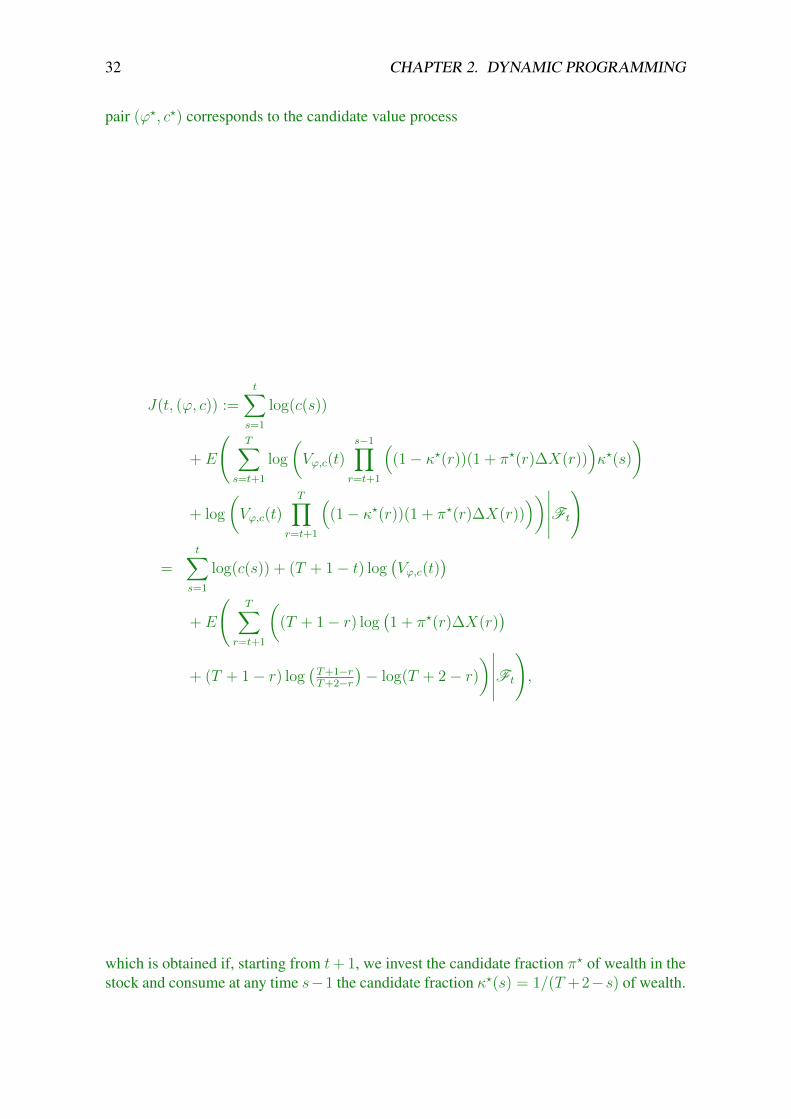
32 CHAPTER 2. DYNAMIC PROGRAMMING
pair (ϕ?, c?) corresponds to the candidate value process
J(t, (ϕ, c)) :=t∑
s=1
log(c(s))
+ E
(T∑
s=t+1
log
(Vϕ,c(t)
s−1∏r=t+1
((1− κ?(r))(1 + π?(r)∆X(r))
)κ?(s)
)
+ log
(Vϕ,c(t)
T∏r=t+1
((1− κ?(r))(1 + π?(r)∆X(r))
))∣∣∣∣∣Ft
)
=t∑
s=1
log(c(s)) + (T + 1− t) log(Vϕ,c(t)
)+ E
(T∑
r=t+1
((T + 1− r) log
(1 + π?(r)∆X(r)
)+ (T + 1− r) log
(T+1−rT+2−r
)− log(T + 2− r)
)∣∣∣∣∣Ft
),
which is obtained if, starting from t+ 1, we invest the candidate fraction π? of wealth in thestock and consume at any time s−1 the candidate fraction κ?(s) = 1/(T +2−s) of wealth.
33
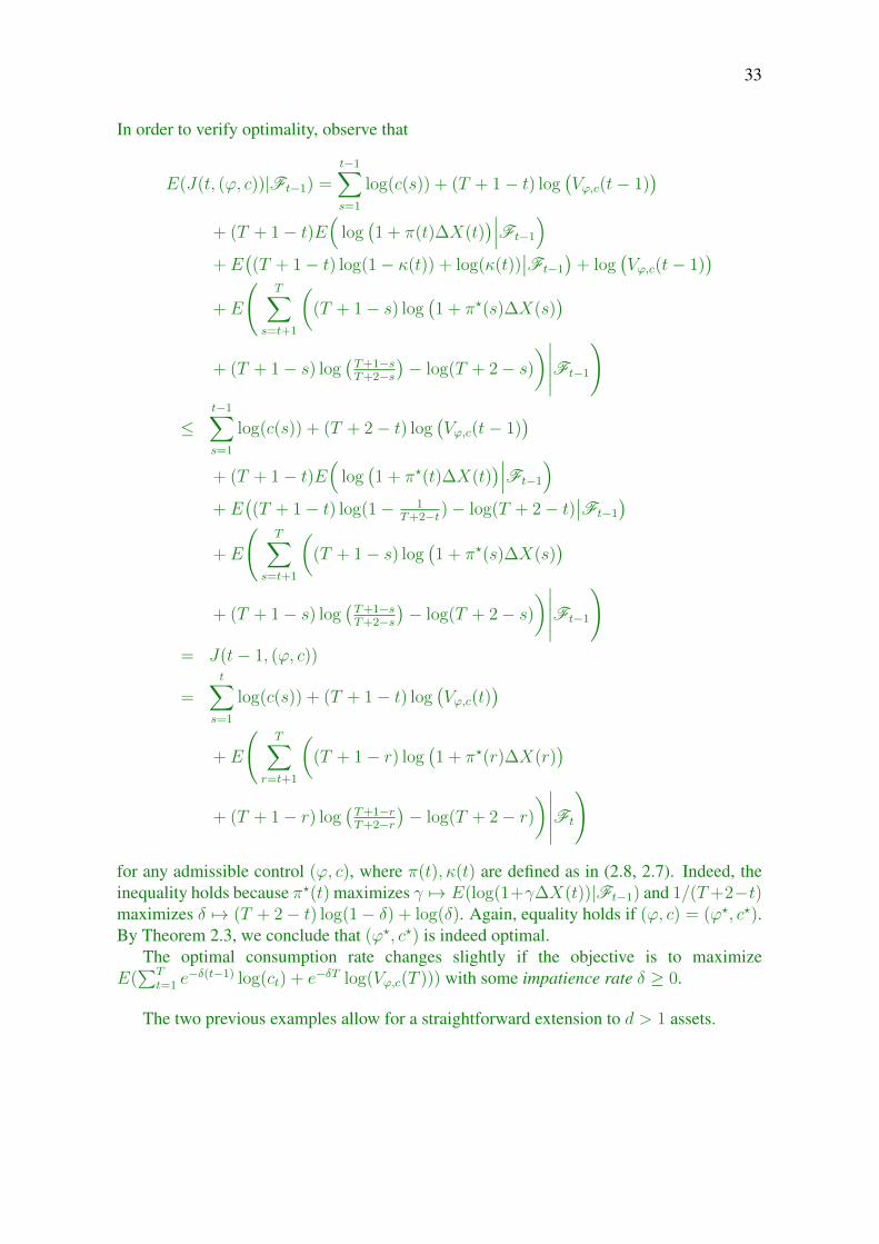
In order to verify optimality, observe that
E(J(t, (ϕ, c))|Ft−1) =t−1∑s=1
log(c(s)) + (T + 1− t) log(Vϕ,c(t− 1)
)+ (T + 1− t)E
(log(1 + π(t)∆X(t)
)∣∣∣Ft−1
)+ E
((T + 1− t) log(1− κ(t)) + log(κ(t))
∣∣Ft−1
)+ log
(Vϕ,c(t− 1)
)+ E
(T∑
s=t+1
((T + 1− s) log
(1 + π?(s)∆X(s)
)+ (T + 1− s) log
(T+1−sT+2−s
)− log(T + 2− s)
)∣∣∣∣∣Ft−1
)
≤t−1∑s=1
log(c(s)) + (T + 2− t) log(Vϕ,c(t− 1)
)+ (T + 1− t)E
(log(1 + π?(t)∆X(t)
)∣∣∣Ft−1
)+ E
((T + 1− t) log(1− 1
T+2−t)− log(T + 2− t)∣∣Ft−1
)+ E
(T∑
s=t+1
((T + 1− s) log
(1 + π?(s)∆X(s)
)+ (T + 1− s) log
(T+1−sT+2−s
)− log(T + 2− s)
)∣∣∣∣∣Ft−1
)= J(t− 1, (ϕ, c))
=t∑
s=1
log(c(s)) + (T + 1− t) log(Vϕ,c(t)
)+ E
(T∑
r=t+1
((T + 1− r) log
(1 + π?(r)∆X(r)
)+ (T + 1− r) log
(T+1−rT+2−r
)− log(T + 2− r)
)∣∣∣∣∣Ft
)
for any admissible control (ϕ, c), where π(t), κ(t) are defined as in (2.8, 2.7). Indeed, theinequality holds because π?(t) maximizes γ 7→ E(log(1+γ∆X(t))|Ft−1) and 1/(T+2−t)maximizes δ 7→ (T + 2− t) log(1− δ) + log(δ). Again, equality holds if (ϕ, c) = (ϕ?, c?).By Theorem 2.3, we conclude that (ϕ?, c?) is indeed optimal.
The optimal consumption rate changes slightly if the objective is to maximizeE(∑T
t=1 e−δ(t−1) log(ct) + e−δT log(Vϕ,c(T ))) with some impatience rate δ ≥ 0.
The two previous examples allow for a straightforward extension to d > 1 assets.

Chapter 3
Optimal Stopping
An important subclass of control problems concerns optimal stopping, i.e. given some timehorizon T and some adapted process X with E(supt∈0,...,T |X(t)|) < ∞, the goal is tomaximise the expected reward
τ 7→ E(X(τ)) (3.1)
over all stopping times τ with values in 0, . . . , T.
Remark 3.1 In the spirit of Chapter 2, a stopping time τ can be identified with the cor-responding adapted process α(t) := 1t≤τ, and hence X(τ) = X(0) + α • X(T ).Put differently, A := α predictable: α 0, 1-valued, decreasing, α(0) = 1 andu(α) := X(0) + α • X(T ) in Chapter 2 lead to the above optimal stopping problem.
Definition 3.2 The Snell envelope of X is the adapted process V defined as
V (t) := ess supE(X(τ)|Ft) : τ stopping time with values in t, t+ 1, . . . , T
. (3.2)
The Snell envelope represents the maximal expected reward if we start at time t and havenot stopped yet. The following martingale criterion may be helpful to verify the optimalityof a candidate stopping time. We will apply its continuous-time version it in two examplesin Chapter 8.
Proposition 3.3 1. Let τ be a stopping time with values in 0, . . . , T. If V is anadapted process such that V τ is a martingale, V (τ) = X(τ), and V (0) = M(0)for some martingale (or at least supermartingale) M ≥ X , then τ is optimal for (3.1)and V coincides up to time τ with the Snell envelope of Definition 3.2.
2. More generally, let τ be a stopping time with values in t, . . . , T and A ∈ Ft. IfV is an adapted process such that V τ − V t is a martingale, V (τ) = X(τ), andV (t) = M(t) onA for some martingale (or at least supermartingale)M withM ≥ Xon A, then V (s) coincides on A for t ≤ s ≤ τ with the Snell envelope of Definition3.2 and τ is optimal on A for (3.2), i.e. it maximises E(X(τ)|Ft) on A.
Proof.
1. This follows from the second statement.
34

35
2. Let s ∈ t, . . . , T. We have to show that
V (s) = ess supE(X(τ)|Fs) : τ stopping time with values in s, . . . , T
holds on s ≤ τ.“≤”: On s ≤ τ ∩ A we have
V (s) = E(V τ (T )|Fs)
= E(X(τ ∨ s)|Fs)
≤ ess supE(X(τ)|Fs) : τ stopping time with values in s, . . . , T
.
(3.3)
“≥”: Note that V τ (T ) = V (τ) = X(τ) ≤M(τ) = M τ (T ) and Lemma 1.6 yield
V τ (s) = M τ (s) ≥ E(M(τ)|Fs) ≥ E(X(τ)|Fs) (3.4)
on s ≤ τ ∩ A for any stopping time τ ≥ s.
(3.3) and (3.4) yield that τ is optimal on A. Indeed, E(X(τ)|Ft) = V (t) ≥E(X(τ)|Ft) holds for any stopping time τ ≥ s.
The following more common verification result correponds to Theorem 2.3 in the frame-work of optimal stopping.
Theorem 3.4 1. Let τ be a stopping time with values in 0, . . . , T. If V ≥ X is asupermartingale such that V τ is a martingale and V (τ) = X(τ), then τ is optimalfor (3.1) and V coincides on up to time τ with the Snell envelope of Definition 3.2.
2. More generally, let τ be a stopping time with values in t, . . . , T. If V ≥ X is anadapted process such that V − V t is a supermartingale, V τ − V t is a martingale,and V (τ) = X(τ), then V (s) coincides for s ≤ t ≤ τ with the Snell envelope ofDefinition 3.2 and τ is optimal for (3.2), i.e. it maximises E(X(τ)|Ft).
3. If τ is optimal for (3.2) and V denotes the Snell envelope, they have the properties instatement 2.
Proof.
1. This follows from the second statement.
2. This immediately follows from choosingM = V in statement 2 of Proposition 3.3 butwe give a short direct proof as well. For any competing stopping time τ with valuesin t, t+ 1, . . . , T, Lemma 1.4 yields
E(X(τ)|Ft) ≤ E(V (τ)|Ft) ≤ V (t),
with equality everywhere for τ = τ .

36 CHAPTER 3. OPTIMAL STOPPING
3. τ ≥ t, V ≥ X and adaptedness of V are obvious. It remains to be shown thatV − V t is a supermartingale, V τ − V t is a martingale, and V (τ) = X(τ). Using theidentification of Remark 3.1, we have V (t) = J(t, 1). Theorem 2.3(1) yields that Vand hence also V − V t are supermartingales. In particular, V (t) ≥ E(V (τ)|Ft). Butoptimality of τ implies
V (t) = E(X(τ)|Ft) ≤ E(V (τ)|Ft). (3.5)
Hence, equality holds in (3.5), which yields X(τ) = V (τ) as well as E(V τ (T ) −V t(T )) = 0 = V τ (0)−V t(0). The martingale property of V τ −V t follows now fromLemma 1.5.
Remark 3.5 Statement 3 in Theorem 3.4 shows that the sufficient conditions in Proposition3.3 are necessary, i.e. for the Snell envelope V there exists a martingale M as in statements1 resp. 2 of this proposition. Indeed, one may choose M := V (0) + MV if V = V (0) +MV + AV denotes the Doob decomposition of V .
Hence, Proposition 3.3 can in principle be used to determine the Snell envelope nu-merically, namely by minimizing M(0) over all martingales dominating X . The resultingprocess coincides with the Snell envelope up to time τ . Cf. also Remark 9.7 in this context.
The following result helps to determine both the Snell envelope and an optimal stoppingtime.
Theorem 3.6 Let V denote the Snell envelope.
1. V is the smallest supermartingale dominating X .
2. V is obtained recursively by V (T ) = X(T ) and
V (t− 1) = maxX(t− 1), E(V (t)|Ft−1)
, t = T − 1, . . . , 0. (3.6)
3. The stopping times
τ t := infs ∈ t, . . . , T : V (s) = X(s)
and
τ t := T ∧ infs ∈ t, . . . , T − 1 : E(V (s+ 1)|Fs) < X(s)
(3.7)
are optimal in (3.2), i.e. they maximise E(X(τ)|Ft).
Proof.
2 and 3. Define V recursively as in statement 2 rather than as in Definition 3.2 andset τ = τ t or τ = τ t. We show that τ and V satisfy the conditions of Theorem3.4(2). It is obvious that V is a supermartingale with V ≥ X and V (τ) = X(τ). Fixs ∈ t+ 1, t+ 2, . . . , T. On the set s ≤ τ we have V (s− 1) = E(V (s)|Fs−1) bydefinition of τ . Hence V τ − V t is a martingale.
37
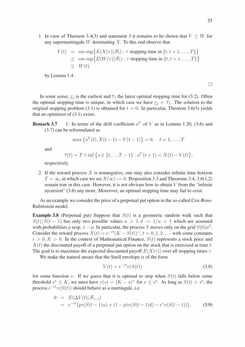
1. In view of Theorem 3.4(3) and statement 3 it remains to be shown that V ≤ W forany supermartingale W dominating X . To this end observe that
V (t) = ess supE(X(τ)|Ft) : τ stopping time in t, t+ 1, . . . , T
≤ ess sup
E(W (τ)|Ft) : τ stopping time in t, t+ 1, . . . , T
≤ W (t)
by Lemma 1.4.
In some sense, τ t is the earliest and τ t the latest optimal stopping time for (3.2). Oftenthe optimal stopping time is unique, in which case we have τ t = τ t. The solution to theoriginal stopping problem (3.1) is obtained for t = 0. In particular, Theorem 3.6(3) yieldsthat an optimizer of (3.1) exists.
Remark 3.7 1. In terms of the drift coefficient aV of V as in Lemma 1.20, (3.6) and(3.7) can be reformulated as
maxaV (t), X(t− 1)− V (t− 1)
= 0, t = 1, . . . , T
andτ(t) = T ∧ inf
s ∈ t, . . . T − 1 : aV (t+ 1) < X(t)− V (t)
,
respectively.
2. If the reward process X is nonnegative, one may also consider infinite time horizonT =∞, in which case we setX(∞) := 0. Proposition 3.3 and Theorems 3.4, 3.6(1,2)remain true in this case. However, it is not obvious how to obtain V from the “infiniterecursion” (3.6) any more. Moreover, an optimal stopping time may fail to exist.
As an example we consider the price of a perpetual put option in the so-called Cox-Ross-Rubinstein model.
Example 3.8 (Perpetual put) Suppose that S(t) is a geometric random walk such thatS(t)/S(t − 1) has only two possible values u > 1, d := 1/u < 1 which are assumedwith probabilities p resp. 1− p. In particular, the process S moves only on the grid S(0)uZ.Consider the reward process X(t) = e−rt(K − S(t))+, t = 0, 1, 2, . . . with some constantsr > 0, K > 0. In the context of Mathematical Finance, S(t) represents a stock price andX(t) the discounted payoff of a perpetual put option on the stock that is exercised at time t.The goal is to maximise the expected discounted payoff E(X(τ)) over all stopping times τ .
We make the natural ansatz that the Snell envelope is of the form
V (t) = e−rtv(S(t)) (3.8)
for some function v. If we guess that it is optimal to stop when S(t) falls below somethreshold s? ≤ K, we must have v(s) = (K − s)+ for s ≤ s?. As long as S(t) > s?, theprocess e−rtv(S(t)) should behave as a martingale, i.e.
0 = E(∆V (t)|Ft−1)
= e−rt(pv(S(t− 1)u) + (1− p)v(S(t− 1)d)− erv(S(t− 1))
), (3.9)
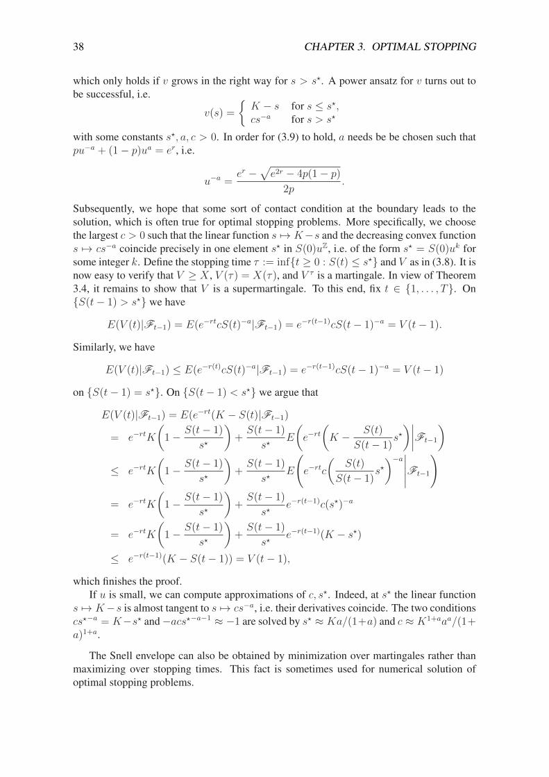
38 CHAPTER 3. OPTIMAL STOPPING
which only holds if v grows in the right way for s > s?. A power ansatz for v turns out tobe successful, i.e.
v(s) =
K − s for s ≤ s?,cs−a for s > s?
with some constants s?, a, c > 0. In order for (3.9) to hold, a needs be be chosen such thatpu−a + (1− p)ua = er, i.e.
u−a =er −
√e2r − 4p(1− p)
2p.
Subsequently, we hope that some sort of contact condition at the boundary leads to thesolution, which is often true for optimal stopping problems. More specifically, we choosethe largest c > 0 such that the linear function s 7→ K−s and the decreasing convex functions 7→ cs−a coincide precisely in one element s? in S(0)uZ, i.e. of the form s? = S(0)uk forsome integer k. Define the stopping time τ := inft ≥ 0 : S(t) ≤ s? and V as in (3.8). It isnow easy to verify that V ≥ X , V (τ) = X(τ), and V τ is a martingale. In view of Theorem3.4, it remains to show that V is a supermartingale. To this end, fix t ∈ 1, . . . , T. OnS(t− 1) > s? we have
E(V (t)|Ft−1) = E(e−rtcS(t)−a|Ft−1) = e−r(t−1)cS(t− 1)−a = V (t− 1).
Similarly, we have
E(V (t)|Ft−1) ≤ E(e−r(t)cS(t)−a|Ft−1) = e−r(t−1)cS(t− 1)−a = V (t− 1)
on S(t− 1) = s?. On S(t− 1) < s? we argue that
E(V (t)|Ft−1) = E(e−rt(K − S(t)|Ft−1)
= e−rtK
(1− S(t− 1)
s?
)+S(t− 1)
s?E
(e−rt
(K − S(t)
S(t− 1)s?)∣∣∣∣Ft−1
)≤ e−rtK
(1− S(t− 1)
s?
)+S(t− 1)
s?E
(e−rtc
(S(t)
S(t− 1)s?)−a∣∣∣∣∣Ft−1
)
= e−rtK
(1− S(t− 1)
s?
)+S(t− 1)
s?e−r(t−1)c(s?)−a
= e−rtK
(1− S(t− 1)
s?
)+S(t− 1)
s?e−r(t−1)(K − s?)
≤ e−r(t−1)(K − S(t− 1)) = V (t− 1),
which finishes the proof.If u is small, we can compute approximations of c, s?. Indeed, at s? the linear function
s 7→ K−s is almost tangent to s 7→ cs−a, i.e. their derivatives coincide. The two conditionscs?−a = K−s? and−acs?−a−1 ≈ −1 are solved by s? ≈ Ka/(1+a) and c ≈ K1+aaa/(1+a)1+a.
The Snell envelope can also be obtained by minimization over martingales rather thanmaximizing over stopping times. This fact is sometimes used for numerical solution ofoptimal stopping problems.

39
Proposition 3.9 The Snell envelope V of X satisfies
V (0) = min
E
(sup
t=0,...,T(X(t)−M(t))
): M martingale with M(0) = 0
and, more generally,
V (t) = min
E
(sup
s=t,...,T(X(s)−M(s))
∣∣∣∣Ft
): M martingale with M(t) = 0
for any t ∈ 0, . . . , T.
Proof. The first statement follows from the second one.“≤”: If τ is a stopping time with values in t, . . . , T, the optional sampling theorem
yields
E(X(τ)|Ft) ≤ E(X(τ)−M(τ)|Ft) ≤ E
(sup
s=t,...,T(X(s)−M(s))
∣∣∣∣Ft
)Since V (t) is the supremum of all such expressions, we have V (τ) ≤ min. . . .
“≥”: Since V is a supermartingale, the predictable part AV in its Doob decompositionV = V (0) +MV + AV is decreasing. The desired inequality follows from
E
(sup
s=t,...,T
(X(s)−MV (s) +MV (t)
)∣∣∣∣Ft
)= E
(sup
s=t,...,T
(X(s)− V (s) + V (0) + AV (s) +MV (t)
)∣∣∣∣Ft
)≤ E
(sup
s=t,...,T
(V (0) + AV (s) +MV (t)
)∣∣∣∣Ft
)= E(V (t)|Ft) = V (t).

Chapter 4
Markovian situation
Above we have derived results that help to prove that a candidate solution is optimal. How-ever, it is not obvious yet how to come up with a reasonable candidate. A standard approachin a Markovian setup is to assume that the value process is a function of the state variablesand to derive a recursive equation for this function — the so-called Bellman equation.
We consider the setup of Chapter 2 with a reward function as in Example 2.1. Supposethat the conditional jump distribution K(α) as in Definition 1.17 of the controlled processX(α) is of Markovian type in the sense thatK(α)(t, ·) depends on α only throughX(α)(t−1)and α(t), i.e.
K(α)(t, ·) = κ(α(t), t, X(α)(t− 1), ·) (4.1)
for some deterministic function κ. Moreover, assume that — up to some measurability orintegrability conditions — the set of admissible controls contains essentially all predictableprocesses with values in some set A ⊂ Rm. The initial value X(α) is supposed to coincidefor all controls α. Under these conditions, it is natural to assume that the value process is ofthe form
J(t, α) =t∑
s=1
f(s,X(α)(s− 1), α(s)) + v(t,X(α)(t)) (4.2)
for some so-called value function v : 0, 1, . . . , T × Rd → R of the control problem.Indeed, what else should the optimal expected future reward depend on?
In order for the supermartingale/martingale conditions from Theorem 2.3 to hold, weneed that
E(J(t, α)− J(t− 1, α)|Ft−1)
= f(t,X(α)(t− 1), α(t)) + E(v(t,X(α)(t))− v(t− 1, X(α)(t− 1))|Ft−1)
= f(t,X(α)(t− 1), α(t))
+
∫ (v(t,X(α)(t− 1) + y)− v(t,X(α)(t− 1))
)κ(α(t), t, X(α)(t− 1), dy)
+ v(t,X(α)(t− 1))− v(t− 1, X(α)(t− 1)) (4.3)= (f (α(t)) +G(α(t))v + ∆tv)(t,X(α)(t− 1)) (4.4)
is nonpositive for any control α and zero for some control α where we used the notation
(G(a)u)(t, x) :=
∫u(t, x+ y)κ(a, t, x, dy)− u(t, x), (4.5)
40

41
∆tu(t, x) := u(t, x)− u(t− 1, x), (4.6)
andf (a)(t, x) := f(t, x, a).
These considerations lead to the following result.
Theorem 4.1 As noted above we assume that there is some deterministic function κ suchthat
E(1B(∆X(α)(t))
∣∣Ft−1
)= κ(α(t), t, X(α)(t− 1), B), (4.7)
α ∈ A , t ∈ 1, . . . , T, B ⊂ Rd. In addition, let A ⊂ Rm be such that any admissiblecontrol is A-valued.
Suppose that function v : 0, 1, . . . , T × Rd → R satisfies
v(T, x) = g(x), (4.8)
the Bellman equation
supa∈A
(f (a) +G(a)v + ∆tv)(t, x) = 0, t = 1, 2, . . . , T, (4.9)
and
α?(t) = argmaxa∈A(f (a) +G(a)v + ∆tv)(t,X(α?)(t− 1)), t = 1, 2, . . . , T (4.10)
for some admissible control α?, where we once more used the notation (4.5). Then α? isoptimal and (4.2) is the value process with corresponding value function v.
Proof. Define (J(·, α))α∈A as in (4.2). The initial value J(0, α) coincides for all controlsα by assumption. (4.8) implies that J(T, α) = u(α). Equations (4.9) and (4.3) yield thatJ(·, α) is a supermartingale for any admissible control. Similarly, (4.9, 4.10, 4.3) imply themartingale property of J(·, α?). The assertion follows now from Theorem 2.3.
Note that the Bellman equation (4.9) allows to compute the value function v(t, ·) recur-sively starting from t = T , namely via v(T, x) = g(x) and
v(t− 1, x) = supa∈A
(f (a)(t, x) +
∫v(t, x+ y)κ(a, t, x, dy)
). (4.11)
Remark 4.2 In the situation of Theorem 4.1, the value function is the smallest function vsatisfying (4.8) and
(f (a) +G(a)v + ∆tv)(t, x) ≤ 0, t = 1, 2, . . . , T (4.12)
for any a ∈ A. Indeed, this follows recursively starting from t = T because (4.12) meansthat
v(t− 1, x) ≥ supa∈A
(f (a)(t, x) +
∫v(t, x+ y)κ(a, t, x, dy)
)and equality holds for the value function.

42 CHAPTER 4. MARKOVIAN SITUATION
Remark 4.3 (Semi-Markovian case) A careful analysis shows that we do not fully need theMarkovian structure (4.1) resp. (4.7) for the above approach to work. Suppose that κ in (4.1)resp. (4.7) depend explicitly on ω in an Ft−1-measurable way. Likewise we allow the valuefunction to be a function v : Ω×0, . . . , T×Rd → R, assumed to be Ft−1-measurable inits first argument ω. Then all of the above remains true, in particular Theorem 4.1, equation(4.11), and Remark 4.2. However, it may be less obvious how to obtain the value functionfrom the recursion (4.11) unless it depends on ω in a simple way.
As an illustration we consider variations of Examples 2.5 and 2.6 for power instead oflogarithmic utility functions.
Example 4.4 (Power utility of terminal wealth) We consider the same problem as in Exam-ple 2.5 but with power utility function u(x) = x1−p/(1− p) for some p ∈ (0,∞) \ 1, i.e.the investor’s goal is to maximise E(u(Vϕ(T ))) over all investment strategies ϕ. In orderto derive explicit solutions we assume that the stock price S(t) = S(0)E (X)(t) follows ageometric random walk.
The set of controls in Example 2.5 is not of the “myopic” form assumed in the beginningof this section. Therefore we consider again relative portfolios π(t), which represent thefraction of wealth invested in the stock, i.e. (2.2). By slight abuse of notation, we writeV (π)(t) for the wealth generated from the investment strategy π, which evolves as
V (π)(t) = v0
t∏s=1
(1 + π(s)∆X(s)
)= v0E (π • X)(t),
cf. (2.3). In order for wealth to stay nonnegative, π(t) needs to be A-valued for
A :=a ∈ R : 1 + ax ≥ 0 for any x in the support of ∆X(1)
,
i.e. we consider the set
A =π predictable : π(0) = 0 and π(t) ∈ A, t = 1, . . . , T
.
(4.9) reads assupa∈A
E(v(t, x(1 + a∆X(1))
))− v(t− 1, x) = 0. (4.13)
We guess that v factors in functions of t and x, respectively. Since the terminal condition(4.8) is v(T, x) = u(x), this leads to the ansatz v(t, x) = g(t)u(x) = g(t)x1−p/(1 − p) forsome function g with g(T ) = 1. Inserting into (4.13) yields
supa∈A
E((1 + a∆X(1))1−p) g(t) = g(t− 1),
which is solved by g(t) = %T−t for
% := E((1 + a?∆X(1))1−p)
anda? := argmaxa∈AE
((1 + a∆X(1))1−p)
Theorem 4.1 now yields that the constant deterministic strategy π?(t) = a? is optimal andthat the value function is indeed of product form v(t, x) = %T−tu(x).
Summing up, it is optimal to invest a fixed fraction of wealth in the stock. The optimalfraction depends on both the law of ∆X(1) and parameter p.
43
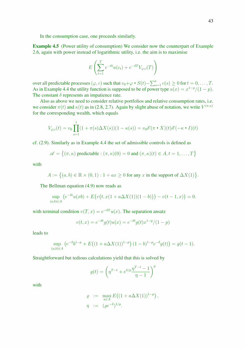
In the consumption case, one proceeds similarly.
Example 4.5 (Power utility of consumption) We consider now the counterpart of Example2.6, again with power instead of logarithmic utility, i.e. the aim is to maximise
E
(T∑t=1
e−δtu(ct) + e−δTVϕ,c(T )
)
over all predictable processes (ϕ, c) such that v0+ϕ • S(t)−∑t
s=1 c(s) ≥ 0 for t = 0, . . . , T .As in Example 4.4 the utility function is supposed to be of power type u(x) = x1−p/(1− p).The constant δ represents an impatience rate.
Also as above we need to consider relative portfolios and relative consumption rates, i.e.we consider π(t) and κ(t) as in (2.8, 2.7). Again by slight abuse of notation, we write V (π,κ)
for the corresponding wealth, which equals
Vϕ,c(t) = v0
t∏s=1
(1 + π(s)∆X(s))(1− κ(s)) = v0E (π • X)(t)E (−κ • I)(t)
cf. (2.9). Similarly as in Example 4.4 the set of admissible controls is defined as
A =
(π, κ) predictable : (π, κ)(0) = 0 and (π, κ)(t) ∈ A, t = 1, . . . , T
with
A :=
(a, b) ∈ R× (0, 1) : 1 + ax ≥ 0 for any x in the support of ∆X(1).
The Bellman equation (4.9) now reads as
sup(a,b)∈A
(e−δtu(xb) + E
(v(t, x(1 + a∆X(1))(1− b)
))− v(t− 1, x)
)= 0.
with terminal condition v(T, x) = e−δTu(x). The separation ansatz
v(t, x) = e−δtg(t)u(x) = e−δtg(t)x1−p/(1− p)
leads to
sup(a,b)∈A
(e−δb1−p + E
((1 + a∆X(1))1−p) (1− b)1−pe−δg(t)
)= g(t− 1).
Straightforward but tedious calculations yield that this is solved by
g(t) =
(ηT−t + eδ/p
ηT−t − 1
η − 1
)pwith
% := maxa∈A
E((1 + a∆X(1))1−p) ,
η := (%e−δ)1/p.

44 CHAPTER 4. MARKOVIAN SITUATION
The optimal controls are π?(t) = a? and κ?(t) = b? with
a? := argmaxa∈AE((1 + a∆X(1))1−p)
as in Example 4.4 and
b? :=(1 + (%g(t))1/p
)−1=
(1 +
ηT−t − 1
η − 1+ %1/pηT−t
)−1
.
Altogether, we observe that the fixed investment fraction from Example 4.4 is still op-timal in the consumption case. The optimal consumption fraction is deterministic and in-creasing over time.
Finally, we reformulate Theorem 4.1 for stopping problems.
Theorem 4.6 Suppose that X(t) = g(Y (t)) for g : Rd → R and some Rd-valued Markovprocess (Y (t))t=1,2,... with generator G in the sense of (1.18). If function v : 0, 1, . . . , T×Rd → R satisfies
v(T, y) = g(y)
and
maxg(y)− v(t− 1, y),∆tv(t, y) +Gv(t, y) = 0, t = 1, 2, . . . , T, (4.14)
then V (t) := v(t, Y (t)), t = 0, . . . , T is the Snell envelope of X . Here we use the notationGv(t, y) := G(v(t, ·))(y) and ∆tv(t, y) = v(t, y)− v(t− 1, y) similarly as in (4.6).
Proof. Since v(T, Y (T )) = g(Y (T )) and
v(t− 1, Y (t− 1)) = v(t− 1, Y (t− 1))
+ maxg(Y (t− 1))− v(t− 1, Y (t− 1)),
v(t, Y (t− 1))− v(t− 1, Y (t− 1)) +Gv(t, Y (t− 1))= maxg(Y (t− 1)), v(t, Y (t− 1)) +Gv(t, Y (t− 1))= maxX(t− 1), E(v(t, Y (t))|Ft−1),
the assertion follows from Theorem 3.6(2).
As in Theorem 4.1, equation (4.14) allows to compute v(t, ·) recursively starting fromt = T , namely via
v(t− 1, y) = max
g(y),
∫v(t, x)P (1, y, dx)
, t = T, . . . , 1, (4.15)
where P (·) denotes the transition function of Y .
Remark 4.7 The function v : 0, 1, . . . , T × Rd → R is Theorem 4.6 is the smallest onethat satisfies v(t, ·) ≥ g(·), t = 0, . . . , T and ∆tv+Gv ≤ 0. Indeed, this follows recursivelyfor t = T, . . . , 0 because these two properties imply
v(t− 1, y) = max
g(y),
∫v(t, x)P (1, y, dx)
,
with equality for the value function by (4.15).
Chapter 5
Stochastic Maximum Principle
We turn now to the counterpart of the first-order conditions in Example 0.1(2). As before,we consider the setup of Chapter 2 with a reward function as in Example 2.1. The set ofadmissible controls A is assumed to contain only predictable processes with values in someconvex set A ⊂ Rm. Moreover, we suppose that the function g is concave.
A sufficient condition for optimality reads as follows:
Theorem 5.1 Suppose that Y is an Rd-valued adapted process and α? an admissible controlwith the following properties, where we suppress as usual the argument ω ∈ Ω in randomfunctions.
1. g is differentiable in X(α?)(T ) with derivative denoted as∇g(X(α?)(T )).
2. For any α ∈ A we have
d∑i=1
(Yi(t− 1)aX
(α)i (t) + cYiX
(α)i (t)
)+ f(t,X(α)(t− 1), α(t)
)(5.1)
= H(t,X(α)(t− 1), α(t)), t = 1, . . . , T
for some function H : Ω× 1, . . . , T × Rd × A → R such that (x, a) 7→ H(t, x, a)is concave and x 7→ H(t, x, α?(t)) is differentiable in X(α?)(t − 1). We denote thederivative as∇xH(t,X(α?)(t− 1), α?(t)) = (∂xiH(t,X(α?)(t− 1), α?(t)))i=1,...,d.
3. The drift rate and the terminal value of Y are given by
aY (t) = −∇xH(t,X(α?)(t− 1), α?(t)), t = 1, . . . , T (5.2)
andY (T ) = ∇g(X(α?)(T )). (5.3)
4. α?(t) maximizes a 7→ H(t,X(α?)(t− 1), a) over A for t = 1, . . . , T .
Then α? is an optimal control, i.e. it maximizes
E
(T∑t=1
f(t,X(α)(t), α(t)) + g(X(α)(T ))
)over all α ∈ A .
45

46 CHAPTER 5. STOCHASTIC MAXIMUM PRINCIPLE
Proof. Let α ∈ A be a competing control. By induction we show that
T∑s=1
E(f(s,X(α)(s− 1), α(s))− f(s,X(α?)(s− 1), α?(s))
∣∣∣Ft
)+ E
(g(X(α)(T ))− g(X(α?)(T )))
∣∣Ft
)≤
t∑s=1
(f(s,X(α)(s− 1), α(s))− f(s,X(α?)(s− 1), α?(s))
)+ Y (t)>
(X(α)(t)−X(α?)(t)
)(5.4)
for t = T, T − 1, . . . , 0. Since X(α)(0) = X(α?)(0), we obtain optimality of α? by insertingt = 0.
In order to verify (5.4) we introduce the notation
h(t, x) := supa∈A
H(t, x, a). (5.5)
We start with t = T . Concavity of g implies
g(X(α)(T ))− g(X(α?)(T )) ≤ Y (T )>(X(α)(T )−X(α?)(T )
), (5.6)
which in turn yields (5.4).For the step from t to t− 1 observe that
E
(f(t,X(α)(t− 1), α(t))− f(t,X(α?)(t− 1), α?(t))
+ Y (t)>(X(α)(t)−X(α?)(t)
)∣∣∣∣Ft−1
)− Y (t− 1)>
(X(α)(t− 1)−X(α?)(t− 1)
)= f(t,X(α)(t− 1), α(t))− f(t,X(α?)(t− 1), α?(t))
+d∑i=1
(X
(α)i (t− 1)aYi(t) + Yi(t− 1)aX
(α)i (t) + cYiX
(α)i (t)
−(X
(α?)i (t− 1)aYi(t) + Yi(t− 1)aX
(α?)i (t) + cYiX
(α?)i (t)
))= H(t,X(α)(t− 1), α(t))−H(t,X(α?)(t− 1), α?(t))
+(X(α)(t− 1)−X(α?)(t− 1)
)>aY (t)
= H(t,X(α)(t− 1), α(t))− h(t,X(α)(t− 1)) (5.7)
+((h(t,X(α)(t− 1)) +X(α)(t− 1)>aY (t)
)−(h(t,X(α?)(t− 1)) +X(α?)(t− 1)
)>aY (t)
)≤ 0,
where the first equality follows from integration by parts, cf. Lemma 1.22. The inequality

47
holds because (5.7) is nonpositive by definition and
h(t,X(α)(t− 1))− h(t,X(α?)(t− 1)) +(X(α)(t− 1)−X(α?)(t− 1)
)>aY (t)
= h(t,X(α)(t− 1))− h(t,X(α?)(t− 1))
−(X(α)(t− 1)−X(α?)(t− 1)
)>∇xh(t,X(α?)(t− 1))
≤ 0
follows from (5.30) and Lemma 0.3.
Remark 5.2 1. On can do without differentiability of g in Theorem 5.1. It is onlyneeded for the estimate in (5.6). Since g is concave, (5.3) can be replaced by theweaker requirement that Y (T ) belongs to the subdifferential of g in X(α?)(T ).
2. The proof shows that concavity of the mapping (x, a) 7→ H(t, x, a) is only needed inorder to apply Lemma 0.3. Instead, we could assume that the mapping x 7→ h(t, x) isconcave and moreover differentiable in X(α?)(t− 1) with derivative
∇xh(t,X(α?)(t− 1)) = ∇xH(t,X(α?)(t− 1), α?(t)). (5.8)
These properties were obtained from Lemma 0.3 if (x, a) 7→ H(t, x, a) is concave.Since α? is the maximizer in (5.5), (5.8) can be expected to hold in more general cir-cumstances. Indeed, consider a real-valued smooth function f(x, y) of two variablesx, y ∈ R and set g(x) := supy f(x, y). If the supremum is attained in y(x), we haveg(x) = f(x, y(x)). The first order condition for y(x) is ∂yf(x, y(x)) = 0. This inturn implies
g′(x) = ∂xf(x, y(x)) + ∂yf(x, y(x))y′(x) = ∂xf(x, y(x)),
which is the analogue of (5.8) in this toy setup.
The first condition in Theorem 5.1 primarily means that the random expression (5.1)depends on the control process α only via the current valuesX(α)(t−1) and α(t). Moreover,this dependence is supposed to be concave unless we are in the more general situation ofRemark 5.2(2). The function H is usually called Hamiltonian. In the deterministic case itreduces to the function with the same name in Example 0.1(2). Similarly, the process Y canbe viewed as a counterpart of the vector y? in that Example.
If additional convexity holds, the process Y solves some dual minimization problem. Weconsider three versions of portfolio optimization problems in Mathematical Finance wherethis is actually the case.
Example 5.3 (Expected utility of terminal wealth) We consider the extension of Exam-ple 2.5 for a general increasing, strictly concave, differentiable utility function u : R →[−∞,∞) (strictly speaking, differentiable in the interior of the half line where it is finite).The investor’s goal is to maximize her expected utility of terminal wealth
E(u(Vϕ(T ))) (5.9)
48 CHAPTER 5. STOCHASTIC MAXIMUM PRINCIPLE
over all controls ϕ ∈ A := ϕ predictable : ϕ(0) = 0 and E(u(Vϕ(T ))) < ∞. Theprocess
Vϕ(t) := v0 + ϕ • S(t), t ∈ [0, T ]
represents the investor’s wealth as in Example 2.5. In this situation the process Y in Theorem5.1 solves some dual convex minimization problem.
Theorem 5.4 1. If Y is a martingale and ϕ? ∈ A such that Y S is a martingale as welland Y (T ) = u′(Vϕ?(T )), then Y and ϕ? satisfy the conditions of Theorem 5.1. Inparticular, ϕ? maximizes (5.9).
2. Suppose that Y and the corresponding optimal control ϕ? are as in Theorem 5.1. ThenY and Y S are martingales satisfying Y (T ) = u′(Vϕ?(T )).
3. Denote the convex dual of u by
u(y) := supx∈R
(u(x)− xy), y ∈ R. (5.10)
Y in Theorem 5.1 minimizes
Z 7→ E(u(Z(T ))) + v0Z(0) (5.11)
among all nonnegative martingales Z such that SZ is a martingale.
4. The optimal values of the primal maximization problem (5.9) and the dual minimiza-tion problem (5.11) coincide in the sense that
E(u(Vϕ?(T ))) = E(u(Y (T ))) + v0Y (0),
where Y and ϕ? ∈ A are processes as in Theorem 5.1 (provided that they exist).
Proof.
1. Since H(t, x, a) = (Y (t − 1)aS(t) + cY S(t))a does not depend on x, we have−∇xH(t, Vϕ?(t − 1), ϕ?(t)) = 0 = aY (t). If Y S is a martingale, we have0 = aY S(t) = S(t− 1)aY (t) + Y (t− 1)aS(t) + cY S(t) and hence H(t, x, a) = 0 forany a. Consequently, Condition 4 in Theorem 5.1 holds as well.
2. As in statement 1, H(t, x, a) = (Y (t − 1)aS(t) + cY S(t))a does not depend on x,which yields aY = 0. Moreover, it is linear in a. In order to have a maximum inϕ?(t) it must vanish, which in turn implies Y (t − 1)aS(t) + cY S(t) = 0 and henceaY S(t) = S(t − 1)aY (t) + Y (t − 1)aS(t) + cY S(t) = 0. Consequently, both Y andY S are local martingales. They are in fact martingales because they are nonnegative.
3. If both Z and ZS are martingales, integration by parts implies that
Vϕ?Z = (v0 + ϕ? • S)Z
= v0Z + Vϕ?−• Z + (Z−ϕ
?) • S + ϕ? • [S,Z]
= v0Z + Vϕ?−• Z + ϕ? • (SZ − S− • Z)
49
and hence E(Vϕ?(T )Z(T )) = v0Z(0) by Lemma 1.10(7). We obtain
E(u(Z(T ))) + v0Z(0)
= E
(supx∈R
(u(x)− xZ(T ))
)+ v0Z(0)
≥ E(u(Vϕ?(T ))− Vϕ?(T )Z(T )) + v0Z(0) (5.12)= E
(u(Vϕ?(T ))
).
Concavity of u yields that x 7→ u(x) − xY (T ) is maximized by Vϕ?(T ) becausethe first-order condition u′(Vϕ?(T )) = Y (T ) holds. Therefore we obtain equality in(5.12) for Z = Y .
4. This follows from the proof of statement 3.
Remark 5.5 Since Y/Y (0) is a positive martingale, it is the density process of a probabilitymeasure Q ∼ P . Since Y S is a martingale, S is a Q-martingale by Lemma 1.15. Such mea-sures Q are called equivalent martingale measures and they play a key role in MathematicalFinance.
Example 5.6 (Expected utility of consumption) As in Example 2.6 we can also considerexpected utility of consumption. Given a constant bond 1 and a stock with price process S,recall that the investor’s wealth is given by
Vϕ,c(t) := v0 + ϕ • S(t)−t∑
s=1
c(s), t ∈ [0, T ],
where ϕ(t) denotes her number of shares in the period from t−1 to t and c(t) the consump-tion at time t− 1. The investor’s goal is to maximize her expected utility
E
(T∑t=1
u(t− 1, c(t)) + u(T, Vϕ,c(T ))
)(5.13)
over all admissible (ϕ, c), where u(t, ·) : R → [−∞,∞), t = 0, . . . , T are increasing,strictly concave, differentiable utility functions as in the previous example. We denote theirderivative by u′(t, ·). Slightly more generally than in Example 2.6 we consider all elementsof
A :=
(ϕ, c) predictable : (ϕ, c)(0) = (0, 0) and
E
(T∑t=1
|u(t− 1, c(t))|+ |u(T, Vϕ,c(T ))|
)<∞
as admissible controls. The counterpart of Theorem 5.7 reads as follows.

50 CHAPTER 5. STOCHASTIC MAXIMUM PRINCIPLE
Theorem 5.7 1. If Y is a martingale and (ϕ?, c?) ∈ A such that Y S is a martingale,Y (t) = u′(t − 1, c?(t)), t = 1, . . . , T , and Y (T ) = u′(T, V (ϕ?,c?)(T )), then Y and(ϕ?, c?) satisfy the conditions of Theorem 5.1. In particular, (ϕ?, c?) maximizes (5.13).
2. Suppose that Y and the corresponding optimal control (ϕ?, c?) are as in Theorem 5.1.Then Y and Y S are martingales satisfying Y (t) = u′(t− 1, c?(t)), t = 1, . . . , T andY (T ) = u′(T, V (ϕ?,c?)(T )).
3. Denote the convex dual of u(t, ·), t = 0, . . . , T by
u(t, y) := supx∈R
(u(t, x)− xy), y ∈ R.
Y in Theorem 5.1 minimizes
Z 7→T∑t=0
E(u(t, Z(t))) + v0Z(0) (5.14)
among all nonnegative martingales Z such that SZ is a martingale.
4. The optimal values of the primal maximization problem (5.13) and the dual minimiza-tion problem (5.14) coincide in the sense that
E
(T∑t=1
u(t− 1, c?(t)) + u(T, V (ϕ?,c?)(T ))
)=
T∑t=0
E(u(t, Y (t))) + v0Y (0),
where Y and (ϕ?, c?) ∈ A are processes as in Theorem 5.1 (provided that they exist.
Proof.
1. Since
H(t, v, (a1, a2)) = (Y (t− 1)aS(t) + cY S(t))a1 − Y (t− 1)a2 + u(t− 1, a2)
in the consumption case, the first statement follows similarly as in Theorem 5.4.
2. The same reasoning as in the proof of Theorem 5.4 yields that Y and Y S are martin-gales. Differentiating H(t, v, (a1, a2)) with respect to a2 yields the first-order condi-tion −Y (t− 1) + u′(t− 1, c?) = 0.

51
3. If Z and ZS are martingales, we have
T∑t=0
E(u(t, Z(t))) + v0Z(0)
=T∑t=0
E
(supx∈R
(u(t, x)− xZ(t))
)+ v0Z(0)
≥T∑t=1
E(u(t− 1, c?(t))− c?(t)Z(t− 1)
)+ E
(u(T, V (ϕ?,c?)(T ))− V (ϕ?,c?)(T )Z(T )
)+ v0Z(0)
=T∑t=1
E(u(t− 1, c?(t))
)+ E
(u(T, V (ϕ?,c?)(T )
)−E
(Z(T )
(V (ϕ?,c?)(T ) +
T∑t=1
c?(t)
))+ v0Z(0)
=T∑t=1
E(u(t− 1, c?(t))
)+ E
(u(T, V (ϕ?,c?)(T )
)−E(Z(T )(v0 + ϕ? • S(T )
)+ v0Z(0)
=T∑t=1
E(u(t− 1, c?(t))
)+ E
(u(T, V (ϕ?,c?)(T )
)because Z(ϕ? • S) is a martingale as well and V (ϕ?,c?)(T ) = v0 + ϕ? • S(T ) −∑T
t=1 c?(t). For Y we have equality because of the first-order conditions listed in
statement 2.
4. This follows from the proof of statement 3.
As in the previous example, Y/Y (0) is the density process of some equivalent martingalemeasure.
Example 5.8 (Expected utility of terminal wealth under proportional transaction costs) Asa third example we return to the above terminal wealth problem, but now in the presenceof proportional transaction costs or, equivalently, differing bid and ask prices. As in Exam-ple 5.3, we consider two assets (bond and stock) with prices 1 and S(t), respectively. Wesuppose that (1 + ε)S(t) must be paid for buying one share of stock at time t, while only(1− ε)S(t) is received for selling one share. For simplicity we assume ε to be fixed.
The investor enters the market with initial endowment v0, entirely invested in bonds. Ifϕ(t) denotes the investor’s number of shares as before, the wealth invested in bonds evolvesaccording to
X(ϕ)0 (t) = v0 −
t∑s=1
(∆ϕ(s)S(s− 1)− ε|∆ϕ(s)|S(s− 1)
),
52 CHAPTER 5. STOCHASTIC MAXIMUM PRINCIPLE
while the wealth in stock amounts to
X(ϕ)1 (t) =
t∑s=1
∆ϕ(s)S(s− 1) + ϕ • S(t) = ϕ(t)S(t). (5.15)
The second equality in (5.15) follows from the integration by parts rule (1.13). The in-vestor’s goal is to maximize expected utility of terminal wealth after liquidation of the stockposition, i.e. to maximize
E(u(X
(ϕ)0 (T ) +X
(ϕ)1 (T )− ε|X(ϕ)
1 (T )|))
(5.16)
over all predictable processes ϕ starting in 0 and such that the expectation (5.16) exists andis finite. In contrast to Example 5.3, we consider the increments ∆ϕ(t) as controls and setA = ∆ϕ predictable : ∆ϕ(0) = 0 and (5.16) exists and is finite.
In order to express the increments ∆X(ϕ)1 (t) in terms of ∆ϕ(t) rather than both ∆ϕ(t)
and ϕ(t), observe that ϕ(t) = ϕ(t− 1) + ∆ϕ(t) and
ϕ(t) =X
(ϕ)1 (t)
S(t), t = 0, . . . , T (5.17)
which yields
∆X(ϕ)1 (t) = ∆ϕ(t)S(t− 1) +
(X
(ϕ)1 (t− 1)
S(t− 1)+ ∆ϕ(t)
)∆S(t)
= ∆ϕ(t)S(t− 1) +X
(ϕ)1 (t)
S(t)∆S(t).
Intuitively, (5.17) holds because the number of shares is the amount invested divided by theprice of the asset. Mathematically, it can be derived from (5.15) because both sides are 0 att = 0 and
X(ϕ)1 (t)
S(t)=
X(ϕ)(t− 1) + ∆ϕ(t)S(t− 1) + ϕ(t)∆S(t)
S(t)
= (ϕ(t− 1) + ∆ϕ(t))S(t− 1)
S(t)+ ϕ(t)
∆S(t− 1)
S(t)
= ϕ(t)
by induction.Similarly as in Examples 5.3 and 5.6, the process Y in Theorem 5.1 can be related
to some minimization problem. More specifically, we obtain the following counterpart ofTheorem 5.4.
Theorem 5.9 1. Suppose that Y0 is a martingale, S a [(1−ε)S, (1+ε)S]-valued processand ϕ? ∈ A such that Y0S is a martingale,
Y0(T ) = u′(v0 + ϕ? • S(T )), (5.18)
andX
(ϕ?)0 (T ) +X
(ϕ?)1 (T )− ε|X(ϕ?)
1 (T )| = v0 + ϕ? • S(T ). (5.19)
Then Y := (Y0,Y0SS
) and ϕ? satisfy the conditions of Theorem 5.1 in the relaxedversion of Remark 5.2(1). In particular, ϕ? maximizes (5.9).
53
2. Suppose that Y = (Y0, Y1) and the corresponding optimal control ϕ? are as in Theo-rem 5.1/Remark 5.2(1). Set S := Y1S/Y0. Then Y0 and Y0S = Y1S are martingales,S is [(1− ε)S, (1 + ε)S]-valued, and (5.18, 5.19) hold.
3. Let Y = (Y0, Y1) be as in Theorem 5.1/Remark 5.2(1). If u denotes the convex dual ofu as in (5.10), (Y0, Y1) minimizes
(Z0, Z1) 7→ E(u(Z0(T ))) + v0Z0(0) (5.20)
among all pairs (Z0, Z1) such that Z0 and Z1S are nonnegative martingales andZ1/Z0 is [1− ε, 1 + ε]-valued.
4. The optimal values of the primal maximization problem (5.16) and the dual minimiza-tion problem (5.20) coincide in the sense that
E(u(X
(ϕ?)0 (T ) +X
(ϕ?)1 (T )− ε|X(ϕ?)
1 (T )|))
= E(u(Y0(T ))) + v0Y0(0),
where Y = (Y0, Y1) and ϕ? ∈ A are processes as in Theorem 5.1 (provided that theyexist).
Proof.
1. Step 1: Firstly, we verify that
X(ϕ?)0 (T ) +X
(ϕ?)1 (T )− ε|X(ϕ?)
1 (T )| ≤ v0 + ϕ? • S(T ) (5.21)
for any adapted [(1− ε)S, (1 + ε)S]-valued process S. Indeed,
X(ϕ?)0 (T ) +X
(ϕ?)1 (T )− ε|X(ϕ?)
1 (T )|
= v0 −T∑t=1
S(t− 1)∆ϕ?(t)(1− sgn(∆ϕ?(t))ε)
+ ϕ?(T )S(T )(1− sgn(ϕ?(T ))ε)
≤ v0 −T∑t=1
S(t− 1)∆ϕ?(t) + ϕ?(T )S(T )
= v0 + S− • ϕ?(T ) + ϕ?(T )S(T )
= v0 + ϕ? • S(T ),
where we used integration by parts for the last step. The above calculation also showsthat equality holds in (5.21) if and only if
∆ϕ?(t)
> 0 only if S(t− 1) = (1− ε)S(t− 1),
< 0 only if S(t− 1) = (1 + ε)S(t− 1)(5.22)
for t = 1, . . . , T and
ϕ?(T )
> 0 only if S(T ) = (1− ε)S(T ),
< 0 only if S(T ) = (1 + ε)S(T ).(5.23)
54 CHAPTER 5. STOCHASTIC MAXIMUM PRINCIPLE
Step 2: Since ϕ(t) = ∆ϕ(t) +X1(t− 1)/S(t− 1), straightforward calculations yieldthat the Hamiltonian equals
H(t, (x0, x1), a) = Y0(t− 1)S(t− 1)(−a− |a|ε) + Y1(t− 1)aS(t− 1)
+(Y1(t− 1)aS(t) + cY1S(t)
) x1
S(t− 1)(5.24)
in this setup.
Step 3: Note that Y1 = S/S has values in [(1− ε)Y0, (1 + ε)Y0] and
Y1(T ) =S(T )
S(T )Y (0) =
(1− ε)Y0(T ) if X(ϕ?)
1 (T ) > 0,
(1 + ε)Y0(T ) if X(ϕ?)1 (T ) < 0
(5.25)
by (5.23).
Step 4: For the application of Theorem 5.1 we need to consider the functiong(x0, x1) := u(x0 + x1 − |x1|ε). It is differentiable in x0 with derivative u′(x0 +x1 − |x1|ε) and in x1 6= 0 with derivative u′(x0 + x1 − |x1|ε)(1 − sgn(x1)ε).Let ∂1g(x0, 0) denote the subdifferential of the concave function x1 7→ g(x0, x1)in x1 = 0. It is easy to see that y1 ∈ ∂1g(x0, 0) holds if and only if y1 ∈[u′(x0 + x1 − |x1|ε)(1 − ε), u′(x0 + x1 − |x1|ε)(1 + ε)]. Together with (5.25) itfollows that Y0(T ) and Y1(T ) satisfy the conditions in (5.3) resp. Remark 5.2(1).
Step 5: Since aY0 = 0 and H(t, (x0, x1), a) does not depend on x0, we obtain thefirst component of the vector-valued equation (5.2). From the martingale property ofY0S = Y1S we conclude 0 = aY1S(t) = Y1(t − 1)aS(t) + cY1S(t) + S(t − 1)aY1(t),which implies aY1(t) = −(Y1(t− 1)aS(t) + cY1S(t))/S(t− 1). This yields the secondcomponent of (5.2).
Step 6: (5.22) can be rephrased as
∆ϕ?(t)
> 0 only if Y1(t− 1) = (1− ε)Y0(t− 1),< 0 only if Y1(t− 1) = (1 + ε)Y0(t− 1).
(5.26)
In view of (5.24), we obtain Condition 4 in Theorem 5.1.
2. Step 1: The martingale property of Y0 follows from (5.2) because H(z, (x0, x1), a)does not depend on x0. The second component of (5.2) yields aY1(t) = −(Y1(t −1)aS(t) + cY1S(t))/S(t − 1) and hence aY1S(t) = Y1(t − 1)aS(t) + cY1S(t) + S(t −1)aY1(t) = 0. Therefore, Y0S = Y1S is a martingale as well.
Step 2: Condition 4 in Theorem 5.1 together with (5.24) yields that S/S = Y1/Y0
must have values in [1− ε, 1 + ε] and that (5.26) holds, which in turn implies (5.22).
Step 3: From (5.3) and the arguments in step 4 above we conclude
Y0(T ) = X(ϕ?)0 (T ) +X
(ϕ?)1 (T )− ε|X(ϕ?)
1 (T )|
and (5.25), which in turn implies (5.23). From step 1 of the first part of the proof weobtain (5.18, 5.19).

55
3. For (Z0, Z1) as in statement 3 of Theorem 5.1 set SZ := SZ1/Z0. From step 1 of thefirst part of the proof we obtain
v0 + ϕ? • S(T ) ≤ v0 + ϕ? • SZ(T )
and hence
E(u(Z0(T ))) + v0Z0(0)
= E
(supx∈R
(u(x)− xZ0(T ))
)+ v0Z0(0)
≥ E(u(v0 + ϕ? • S(T ))− (v0 + ϕ? • S(T ))Z0(T )
)+ v0Z(0) (5.27)
≥ E(u(v0 + ϕ? • S(T ))− (v0 + ϕ? • SZ(T ))Z0(T )
)+ v0Z(0) (5.28)
= E(u(X
(ϕ?)0 (T ) +X
(ϕ?)1 (T )− ε|X(ϕ?)
1 (T )|)).
For (Z0, Z1) = (Y0, Y1), equality holds in (5.27, 5.28) by (5.18, 5.19) and step 1 ofthe first part of the proof.
4. This follows from the proof of statement 3.
Remark 5.10 Consider a frictionless price process S without transaction costs satisfying(1− ε)S(t) ≤ S(t) ≤ (1 + ε)S(t) at any time t. Since this asset can be bought cheaper andsold more expensively than the original S, trading S should lead to higher terminal wealthand hence expected utility. Suppose now that the utility-maximizing investment ϕ? in themarket S only buys shares when S = (1+ε)S and sells when S = (1−ε)S. Put differently,its terminal liquidation wealth in both markets coincides; it amounts to v0 + ϕ? • S. Thenϕ? must a fortiori be optimal in the market S because the maximal expected utility in thelatter is certainly bounded above by that in the frictionless alternative S.
This is precisely the economical interpretation of the process in the previous theorem.It represents a fictitious frictionless asset such that the optimal portfolio, its terminal wealthand hence expected utility coincide with that of the original market with transaction costs.Indeed, by Theorem 5.4 the martingale property of Y and Y S together with (5.18) yieldoptimality of ϕ? for S and the frictionless terminal wealth problem of Example 5.3.
As a concrete example we reconsider the portfolio problem of Example 2.5. The relatedproblems in Examples 2.6, 4.4, 4.5 can be treated similarly.
Example 5.11 (Logarithmic utility of terminal wealth) We study Example 5.3 for u = logas in Example 2.5. In order to apply Theorem 5.4 we need a candidate optimal control ϕ?
and a candidate process Y with terminal value Y (T ) = u′(Vϕ?(T )) = 1/Vϕ?(T ). We boldlyguess that
Y (t) := 1/Vϕ?(t), t = 0, . . . , T (5.29)
may do the job for some ϕ? ∈ A that is yet to be determined. In order to simplify compu-tations, we write
ϕ?(t) = π?(t)Vϕ(t− 1)
S(t− 1)
56 CHAPTER 5. STOCHASTIC MAXIMUM PRINCIPLE
similarly as in (2.2). Observe that the increment of the compensator of Y equals
aY (t) = E(Y (t)− Y (t− 1)|Ft−1)
= E
(1
Vϕ?(t− 1)(1 + π?(t)∆X(t))− Y (t− 1)
∣∣∣∣Ft−1
)= −Y (t− 1)π?(t)E
(∆X(t)
1 + π?(t)∆X(t)
∣∣∣∣Ft−1
). (5.30)
and hence
aY S(t) = E(Y (t)S(t)− Y (t− 1)S(t− 1)|Ft−1)
= Y (t− 1)S(t− 1)E
(1 + ∆X(t)
1 + π?(t)∆X(t)− 1
∣∣∣∣Ft−1
)= Y (t− 1)S(t− 1)
(1− π?(t)
)E
(∆X(t)
1 + π?(t)∆X(t)
∣∣∣∣Ft−1
)(5.31)
In order for Y and Y S to be martingales, we want both (5.30) and (5.31) to vanish, whichnatually leads to the condition
E
(∆X(t)
1 + π?(t)∆X(t)
∣∣∣∣Ft−1
)= 0 (5.32)
for the optimal fraction π?(t) of wealth. in view of Theorem 5.1, we have found the optimalinvestment strategy.
How does this relate to Example 2.5 where π?(t) was supposed to be the maximizerof (2.4)? Unless the maximum is attained at the boundary, the first-order condition forthe optimizer is precisely (5.32) if we may exchange differentiation and integration. If theoptimizer of (2.4) is at the boundary of the set of fractions γ satisfying 1 + γ∆X(t) ≥ 0almost surely, (5.32) may fail to have a solution ϕ?(t). This means that our present approachdoes not lead to the optimal portfolio in this case.
Semi-Markovian situation
How are the present approach and in particular the process Y related to dynamic program-ming? In general this may not be obvious but in a semi-Markovian framework there is anatural candidate, namely the derivative of the value function evaluated at the optimal con-trolled process. More specifically, we will argue informally that one can often choose
Y (t) = ∇xv(t,X(α?)(t)), (5.33)
where v denotes the value function of Chapter 4 in the relaxed sense of Remark 4.3,∇xv(t, x0) the gradient of x 7→ v(t, x) at any x0, and α? ∈ A an optimal control.
To this end, suppose that the following holds.
1. The objective function g is concave and the state space A of the admissible controls isconvex.
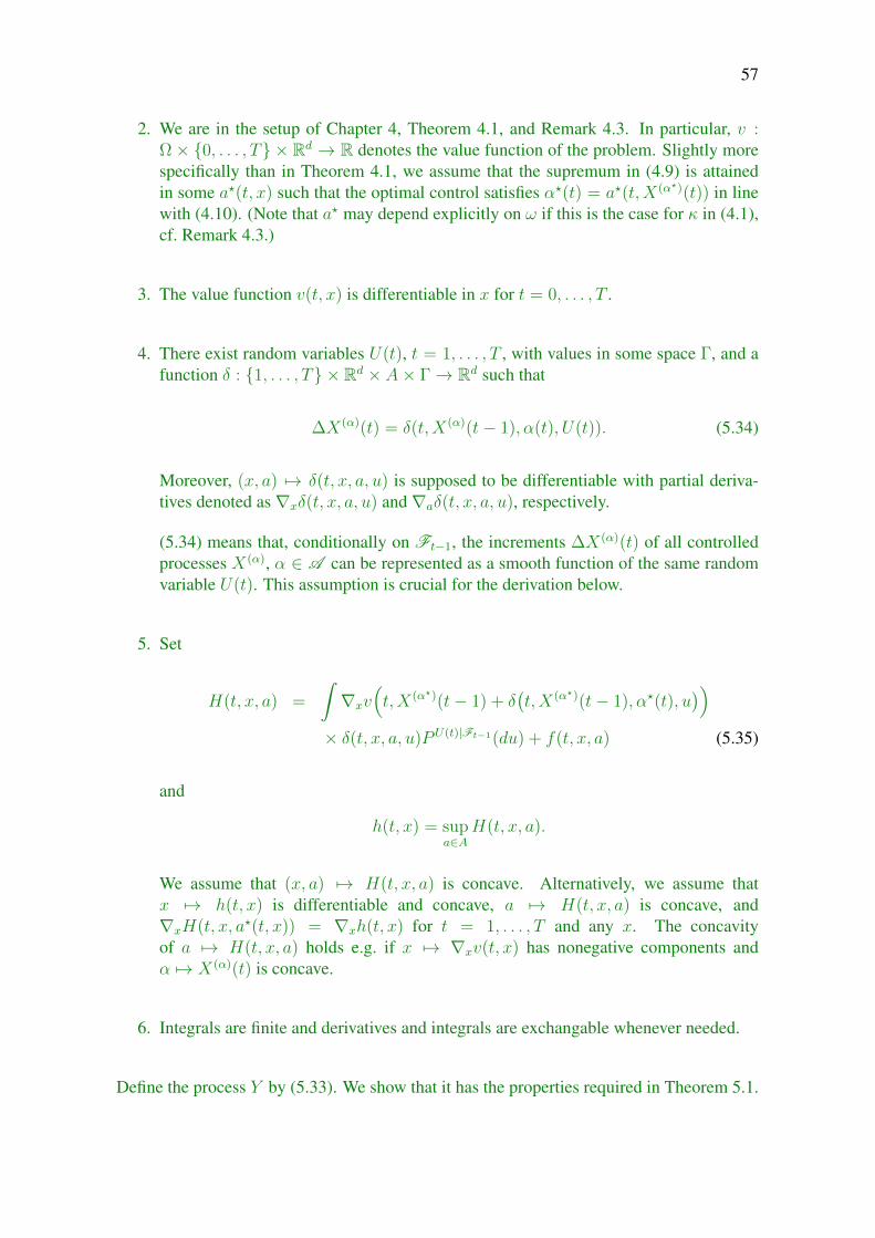
57
2. We are in the setup of Chapter 4, Theorem 4.1, and Remark 4.3. In particular, v :Ω× 0, . . . , T × Rd → R denotes the value function of the problem. Slightly morespecifically than in Theorem 4.1, we assume that the supremum in (4.9) is attainedin some a?(t, x) such that the optimal control satisfies α?(t) = a?(t,X(α?)(t)) in linewith (4.10). (Note that a? may depend explicitly on ω if this is the case for κ in (4.1),cf. Remark 4.3.)
3. The value function v(t, x) is differentiable in x for t = 0, . . . , T .
4. There exist random variables U(t), t = 1, . . . , T , with values in some space Γ, and afunction δ : 1, . . . , T × Rd × A× Γ→ Rd such that
∆X(α)(t) = δ(t,X(α)(t− 1), α(t), U(t)). (5.34)
Moreover, (x, a) 7→ δ(t, x, a, u) is supposed to be differentiable with partial deriva-tives denoted as∇xδ(t, x, a, u) and ∇aδ(t, x, a, u), respectively.
(5.34) means that, conditionally on Ft−1, the increments ∆X(α)(t) of all controlledprocesses X(α), α ∈ A can be represented as a smooth function of the same randomvariable U(t). This assumption is crucial for the derivation below.
5. Set
H(t, x, a) =
∫∇xv
(t,X(α?)(t− 1) + δ
(t,X(α?)(t− 1), α?(t), u
))× δ(t, x, a, u)PU(t)|Ft−1(du) + f(t, x, a) (5.35)
and
h(t, x) = supa∈A
H(t, x, a).
We assume that (x, a) 7→ H(t, x, a) is concave. Alternatively, we assume thatx 7→ h(t, x) is differentiable and concave, a 7→ H(t, x, a) is concave, and∇xH(t, x, a?(t, x)) = ∇xh(t, x) for t = 1, . . . , T and any x. The concavityof a 7→ H(t, x, a) holds e.g. if x 7→ ∇xv(t, x) has nonegative components andα 7→ X(α)(t) is concave.
6. Integrals are finite and derivatives and integrals are exchangable whenever needed.
Define the process Y by (5.33). We show that it has the properties required in Theorem 5.1.
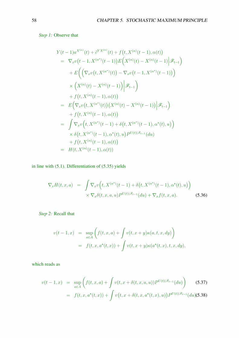
58 CHAPTER 5. STOCHASTIC MAXIMUM PRINCIPLE
Step 1: Observe that
Y (t− 1)aX(α)
(t) + cY X(α)
(t) + f(t,X(α)(t− 1), α(t)
)= ∇xv
(t− 1, X(α?)(t− 1)
)E(X(α)(t)−X(α)(t− 1)
∣∣∣Ft−1
)+ E
((∇xv
(t,X(α?)(t)
)−∇xv
(t− 1, X(α?)(t− 1)
))×(X(α)(t)−X(α)(t− 1)
)∣∣∣∣Ft−1
)+ f(t,X(α)(t− 1), α(t)
)= E
(∇xv
(t,X(α?)(t)
)(X(α)(t)−X(α)(t− 1)
)∣∣∣Ft−1
)+ f(t,X(α)(t− 1), α(t)
)=
∫∇xv
(t,X(α?)(t− 1) + δ
(t,X(α?)(t− 1), α?(t), u
))× δ(t,X(α?)(t− 1), α?(t), u
)PU(t)|Ft−1(du)
+ f(t,X(α)(t− 1), α(t)
)= H(t,X(α)(t− 1), α(t))
in line with (5.1). Differentiation of (5.35) yields
∇xH(t, x, a) =
∫∇xv
(t,X(α?)(t− 1) + δ
(t,X(α?)(t− 1), α?(t), u
))×∇xδ(t, x, a, u)PU(t)|Ft−1(du) +∇xf(t, x, a). (5.36)
Step 2: Recall that
v(t− 1, x) = supa∈A
(f(t, x, a) +
∫v(t, x+ y)κ(a, t, x, dy)
)= f(t, x, a?(t, x)) +
∫v(t, x+ y)κ(a?(t, x), t, x, dy),
which reads as
v(t− 1, x) = supa∈A
(f(t, x, a) +
∫v(t, x+ δ(t, x, a, u))PU(t)|Ft−1(du)
)(5.37)
= f(t, x, a?(t, x)) +
∫v(t, x+ δ(t, x, a?(t, x), u)
)PU(t)|Ft−1(du).(5.38)
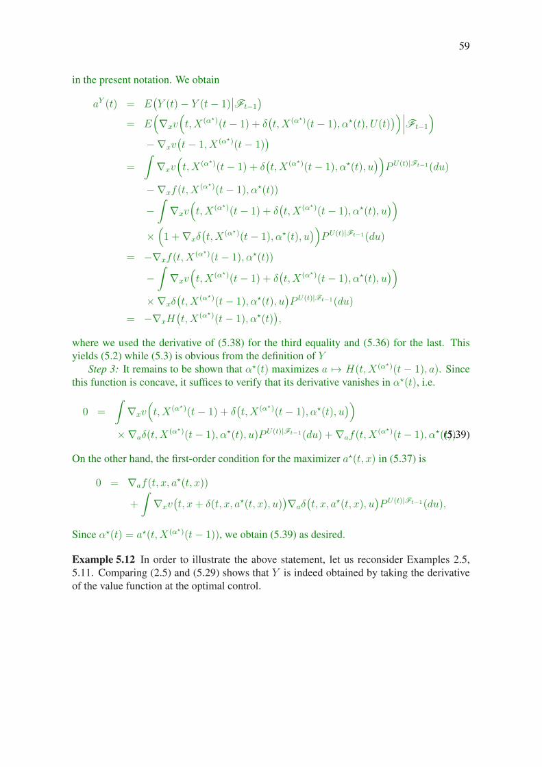
59
in the present notation. We obtain
aY (t) = E(Y (t)− Y (t− 1)
∣∣Ft−1
)= E
(∇xv
(t,X(α?)(t− 1) + δ
(t,X(α?)(t− 1), α?(t), U(t)
))∣∣∣Ft−1
)−∇xv
(t− 1, X(α?)(t− 1)
)=
∫∇xv
(t,X(α?)(t− 1) + δ
(t,X(α?)(t− 1), α?(t), u
))PU(t)|Ft−1(du)
−∇xf(t,X(α?)(t− 1), α?(t))
−∫∇xv
(t,X(α?)(t− 1) + δ
(t,X(α?)(t− 1), α?(t), u
))×(
1 +∇xδ(t,X(α?)(t− 1), α?(t), u
))PU(t)|Ft−1(du)
= −∇xf(t,X(α?)(t− 1), α?(t))
−∫∇xv
(t,X(α?)(t− 1) + δ
(t,X(α?)(t− 1), α?(t), u
))×∇xδ
(t,X(α?)(t− 1), α?(t), u
)PU(t)|Ft−1(du)
= −∇xH(t,X(α?)(t− 1), α?(t)
),
where we used the derivative of (5.38) for the third equality and (5.36) for the last. Thisyields (5.2) while (5.3) is obvious from the definition of Y
Step 3: It remains to be shown that α?(t) maximizes a 7→ H(t,X(α?)(t − 1), a). Sincethis function is concave, it suffices to verify that its derivative vanishes in α?(t), i.e.
0 =
∫∇xv
(t,X(α?)(t− 1) + δ
(t,X(α?)(t− 1), α?(t), u
))×∇aδ(t,X
(α?)(t− 1), α?(t), u)PU(t)|Ft−1(du) +∇af(t,X(α?)(t− 1), α?(t)).(5.39)
On the other hand, the first-order condition for the maximizer a?(t, x) in (5.37) is
0 = ∇af(t, x, a?(t, x))
+
∫∇xv
(t, x+ δ(t, x, a?(t, x), u)
)∇aδ
(t, x, a?(t, x), u
)PU(t)|Ft−1(du),
Since α?(t) = a?(t,X(α?)(t− 1)), we obtain (5.39) as desired.
Example 5.12 In order to illustrate the above statement, let us reconsider Examples 2.5,5.11. Comparing (2.5) and (5.29) shows that Y is indeed obtained by taking the derivativeof the value function at the optimal control.

Part II
Continuous time
60

61
Dynamic stochastic optimization problems play an important role in Mathematical Fi-nance and other applications. In this chapter we provide basic concepts for their mathe-matical treatment in continuous time. We proceed in close correspondence to Part I. Inparticular, we distinguish two approaches, which are discussed in the chapters on dynamicprogramming and the stochastic maximum principle, respectively.

Chapter 6
Recap of stochastic processes
6.1 Continuous semimartingales
6.1.1 Processes, stopping times, martingalesThis section corresponds directly to its discrete counterpart in Chapter 1. As in that casewe work on a fixed filtered probability space (Ω,F ,F, P ). The filtration F = (Ft)t≥0 isnow indexed by continuous time R+ rather than discrete time N. Since information growswith time, we assume Fs ⊂ Ft for s ≤ t as before. Moreover, the filtration is supposed tobe right-continuous in the sense that
Fs =⋂t>s
Ft, s ≥ 0.
Intuitively, this means that no new information arrives immediately after s. One imposesthis rather technical condition to obtain a more streamlined theory.
Collections of real- or vector-valued random variables X = (X(t))t≥0 are again calledstochastic processes. Only the index set N is now replaced by R+. As before, we sometimesview them as real- or vector-valued functions X(ω, t) of two arguments.
Alternatively, they can be seen as single random variables whose values X(ω) are func-tions on the real line. The process X is called continuous, left-continuous etc. if the pathsX(ω) : R+ → R (resp. X(ω) : R+ → Rd) have this property. One mostly works withcàdlàg processes, i.e. processes whose paths are right-continuous and have finite left-handlimits. The french acronym càdlàg stands for continu à droite avec des limites à gauche. IfX is a càdlàg process, its left-hand limits
X−(t) := X(t−) :=
lims↑tX(s) if t > 0,X(0) if t = 0
and its jumps∆X(t) := X(t)−X(t−)
are well defined. Since they are defined for any t, we consider them as stochastic processesX− = (X−(t))t≥0, ∆X = (∆X(t))t≥0 on their own. Observe that X− is a càglàd process,i.e. it is left-continuous and has finite limits from the right. In this introductory course,however, we focus on continuous processes, i.e. we do not allow for jumps.
62
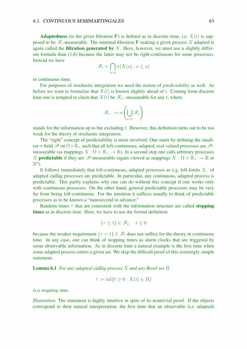
6.1. CONTINUOUS SEMIMARTINGALES 63
Adaptedness (to the given filtration F) is defined as in discrete time, i.e. X(t) is sup-posed to be Ft-measurable. The minimal filtration F making a given process X adapted isagain called the filtration generated by X . Here, however, we must use a slightly differ-ent formula than (1.6) because the latter may not be right-continuous for some processes.Instead we have
Ft =⋂u>t
σ(X(s) : s ≤ u)
in continuous time.For purposes of stochastic integration we need the notion of predictability as well. As
before we want to formalize that X(t) is known slightly ahead of t. Coming from discretetime one is tempted to claim that X(t) be Ft−-measurable for any t, where
Ft− := σ
(⋃s<t
Fs
)
stands for the information up to but excluding t. However, this definition turns out to be tooweak for the theory of stochastic integration.
The “right” concept of predictability is more involved. One starts by defining the small-est σ-field P on Ω×R+ such that all left-continuous, adapted, real-valued processes are P-measurable (as mappings X : Ω× R+ → R). In a second step one calls arbitrary processesX predictable if they are P-measurable (again viewed as mappings X : Ω × R+ → R orRd).
It follows immediately that left-continuous, adapted processes as e.g. left-limits X− ofadapted càdlàg processes are predictable. In particular, any continuous, adapted process ispredictable. This partly explains why one can do without this concept if one works onlywith continuous processes. On the other hand, general predictable processes may be veryfar from being left-continuous. For the intuition it suffices usually to think of predictableprocesses as to be known a “nanosecond in advance.”
Random times τ that are consistent with the information structure are called stoppingtimes as in discrete time. Here, we have to use the formal definition
τ ≤ t ∈ Ft, t ≥ 0
because the weaker requirement τ = t ∈ Ft does not suffice for the theory in continuoustime. In any case, one can think of stopping times as alarm clocks that are triggered bysome observable information. As in discrete time a natural example is the first time whensome adapted process enters a given set. We skip the difficult proof of this seemingly simplestatement.
Lemma 6.1 For any adapted càdlàg process X and any Borel set B,
τ := inft ≥ 0 : X(t) ∈ B
is a stopping time.
Illustration. The statement is highly intuitive in spite of its nontrivial proof. If the objectscorrespond to their natural interpretation, the first time that an observable (i.e. adapted)

64 CHAPTER 6. RECAP OF STOCHASTIC PROCESSES
process enters a given set should certainly be observable itself (i.e. a stopping time).
For technical reasons it is often necessary to stop a process X at a stopping time τ . Asin discrete time, stopping means to keep the process constant from τ on, i.e. we define thestopped process Xτ as
Xτ (t) := X(τ ∧ t).Martingales play an even more important role than in discrete-time stochastic calcu-
lus. Similarly as in Chapter 1 we call an adapted càdlàg process X martingale (resp. sub-martingale, supermartingale) if it is integrable (in the sense that E(|X(t)|) <∞ for anyt) and satisfies
E(X(t)|Fs) = X(s) (resp. ≥ X(s),≤ X(s)) (6.1)
for s ≤ t.
Remark 6.2 Above we assume the càdlàg property as part of the definition of martingalesresp. sub-/supermartingales. If we omit this requirement, we can show that
1. any martingale X has a càdlàg version, i.e. there exists an adapted càdlàg process Xwith X(t) = X(t),
2. any sub-σ-martingale X has a càdlàg version if and only if t 7→ E(X(t)) is rightcontinuous for any t ≥ 0,
cf. [RY99, Theorem II.2.9].
The following technical lemma agrees verbatim with Lemma 1.6. It is needed only forthe proof of Proposition 8.3.
Lemma 6.3 Let X be a supermartingale, Y a martingale, t ≤ T , and A ∈ Ft with X(t) =Y (t) on A and X(T ) ≥ Y (T ). Then X(s) = Y (s) on A for t ≤ s ≤ T . The statementremains to hold if we only requireXT−X t, Y T−Y t instead ofX, Y to be a supermartingaleresp. martingale.
Proof. This follows along the same lines as Lemma 1.6.
As in discrete time, a fair/favourable/unfavourable game remains fair/favourable/ un-favourable if one stops playing at an observable time, cf. Lemma 1.4.
Lemma 6.4 If X is a martingale (resp. submartingale, supermartingale), the same is truefor Xτ if τ denotes an arbitrary stopping time.
Illustration. If τ has only finitely many values t1, . . . , tn, the situation is essentially thesame as in discrete time because only finitely many times are involved. If τ has infinitelymany values, it can be approximated by a sequence (τn)n∈N of stopping times satisfyingτ1 ≥ τ2 ≥ · · · ≥ τn
n→∞−→ τ , namely by setting
τn := inft ≥ τ : t ∈ 1/2n, 2/2n, . . . , n2n/2n
.
Since τn has only finitely many values, we have E(Xτnt |Fs) = Xτn
s , s ≤ t (resp. ≥,≤ forsub-/supermartingales). For n → ∞ the left- resp. right-hand side converge to E(Xt|Fs)
6.1. CONTINUOUS SEMIMARTINGALES 65
and Xs, respectively, because X has right-continuous paths.
Any integrable random variable ξ naturally leads to a martingale via
X(t) = E(ξ|Ft), (6.2)
called again the martingale generated by ξ. Contrary to discrete time, this does not followimmediately from the law of iterated expectations. The proof is complicated by the factthat we assumed càdlàg paths in the definition above. The existence of a càdlàg version of(6.2) relies on martingale convergence theorems and is beyond the scope of this notes. Ifthe random variable generating the martingale is the density of some probability measureQ ∼ P , we obtain again the density process of Q relative to P . We refer to Example 1.7,which extends without change to continuous time.
For the purposes of stochastic calculus we often need the “local” counterpart of the mar-tingale concept, namely local martingales defined below, which reduce to local martingalesin the sense of Chapter 1 in discrete time. However, they do not rely on the intuitive equa-tion (1.9), which does not make sense in continuous time. The way out is to introduce theconcept of localization. Since it is used not only for martingales, we take a more generalperspective.
A class C of processes is called stable under stopping if the stopped processX belongsto C for any X ∈ C . This property holds for most classes of processes considered inthis notes as e.g. martingales, sub-/supermartingales, bounded processes, processes of finitevariation, etc. We say that a process X belongs to the localized class Cloc if there exists asequence of stopping times (τn)n∈N, increasing to∞ almost surely and such that the stoppedprocesses Xτn belong to C for any n.
If the set C is the class of martingales (or e.g. sub-/supermartingales, bounded processes,. . . ), we call the elements of Cloc local martingales (resp. local sub-/supermartingales,locally bounded, . . . ). Roughly speaking, one may say that a local martingale X coincideswith a martingale up to an “arbitrarily large” stopping time τn. Nevertheless, X may behavequite differently from a martingale on a “global” scale. It needs some experience to get agood feeling for the difference between local and true martingales, which is best explainedin a certain lack of uniform integrability. For the time being, it may suffice to think ofa local martingale as almost being a martingale. The fact that not any local martingaleis a martingale leads to many annoying problems in probability theory and MathematicalFinance.
A useful fact in this context is the following
Lemma 6.5 Any nonnegative local martingale is a supermartingale. Any bounded localmartingale is martingale.
Illustration. We show the first statement only for local martingales X . If (τn)n denotes alocalizing sequence for X , Fatou’s lemma and the supermartingale property of Xτn yield
E(X(t)|Fs) = E(
limn→∞
Xτn(t)∣∣∣Fs
)≤ lim inf
n→∞E(Xτn(t)
∣∣Fs
)= Xτn(s) = X(s), s ≤ t.

66 CHAPTER 6. RECAP OF STOCHASTIC PROCESSES
The second statement follows from the first by considering both X and −X , possiblyshifted in order to become nonnegative.
Occasionally, we need the more precise refinement of the previous result.
Lemma 6.6 A local martingale X is a uniformly integrable martingale (i.e. a martingalesuch that X(t) : t ∈ R+ is uniformly integrable) if and only if it is of class (D) (i.e. ifX(τ) : τ finite stopping time is uniformly integrable). If the time domain is [0, T ] insteadof R+, any martingale is in fact uniformly integrable.
A local supermartingale is a supermartingale if it is bounded from below by a processof class (D).
Proof. Step 1: For the first statement let (τn)n∈N denote a corresponding sequence of stop-ping times. From the martingale conditions E(Xτn(t)|Fs) = Xτn(s) for s ≤ t we obtainthe martingale property in the limit n→∞.
Step 2: As in Step 1 one shows that any local supermartingale of class (D) is a super-martingale.
Step 3: If X is a local supermartingale bounded below by a process of class (D),the process X ∧ n is a local supermartingale of class (D) for any n ∈ N. Hence it isa supermartingale by Step 2 and satisfies E(X(t) ∧ n|Fs) ≤ X(s) ∧ n for any s ≤ t.Monotone convergence yields E(X(t)|Fs) ≤ X(s) in the limit for n→∞.
In Chapter 1 we observed the intuitive fact that any submartingale can be decomposedinto a martingale and an increasing compensator representing the trend of the process. Thisstatement has a continuous counterpart:
Lemma 6.7 (Doob-Meyer decomposition) Any continuous submartingale (resp. super-martingale) X can be uniquely decomposed as
X = X(0) +MX + AX (6.3)
with some continuous martingale MX and some increasing (resp. decreasing) process AX
satisfying MX(0) = AX(0) = 0. The process AX is called compensator of X .
Illustration. This statement can be proved by considering a sequence of discrete time sets(t
(k)n )n∈N, k = 1, 2, . . . instead of R+, where the mesh size max|t(k)
n −t(k)n−1| : n = 1, 2, . . .
tends to 0 as k → ∞. The hard part of the proof consists in showing that the discrete-timeDoob decomposition corresponding to the grid (t
(k)n )n∈N converges in an appropriate sense
to a continuous-time decomposition of the required form.
Decompositions of this type play an important role in stochastic calculus, which is whyone wants to extend them to more general classes of processes similar to Lemma 1.8. Con-trary to the discrete case, predictability of the compensator does not suffice to ensure unique-ness of the decomposition. We need an additional path property, namely finite variation.
We say that a real- or vector-valued function α on R+ is of finite variation if its totalvariation on [0, t], i.e.
Var(α)(t) := sup
n∑i=1
|α(ti)− α(ti−1)| : 0 = t0 < t1 < · · · < tn = t
, (6.4)

6.1. CONTINUOUS SEMIMARTINGALES 67
is finite for any finite t ≥ 0. It is not hard to show that a real-valued function α is of finitevariation if and only if it can be written as difference
α = β − γ (6.5)
of two increasing functions β, γ. Indeed, (6.5) implies
Var(α)(t) ≤ β(t) + γ(t) <∞.
Conversely, one may take β := Var(α) if α is of finite variation.In order to provide some intuition, suppose that α(t) denotes the location of a particle at
time t. The total distance covered by the particle between 0 and t is finite if and only if α isof finite variation on [0, t].
A processX is called of finite variation if its pathsX(ω) have this property. In this casethe variation process Var(X) = (Var(X)(t))t≥0 is defined pathwisely. If X is an adaptedcontinuous process, so is Var(X).
Let us come back to extensions of Lemma 6.7. The following result ensures that thereis at most one decomposition (6.3) of a given process X into a martingale and a predictableprocess of finite variation.
Lemma 6.8 Any continuous local martingale X of finite variation is constant, i.e. X(t) =X(0).
Illustration. Since X is of finite variation, it can be written as a difference
X = X(0) + A−B
with increasing processes A,B satisfying A(0) = 0 = B(0). One can show that A and Bcan be chosen adapted and continuous. As an increasing process B is a submartingale ifit is integrable. Lacking integrability is taken care of by considering the stopped processesXτn instead of X , where the stopping times τn are chosen such that Xτn is a sufficientlyintegrable martingale. Observe that B allows for two Doob-Meyer type decompositions
0 +B = B = (X −X(0)) + A.
By uniqueness of the Doob-Meyer decomposition we have 0 = X −X(0) and B = A (cf.Lemma 6.7).
The previous lemma does not answer the question which processes actually allow for arepresentation (6.3). The class of these processes turns out to be quite large if we relax themartingale property of MX slightly. One calls them semimartingales. More specifically,an adapted continuous process X is called (continuous) semimartingale if it allows for adecomposition
X = X(0) +MX + AX (6.6)
with some continuous local martingale MX and some adapted continuous process AX offinite variation satisfying MX(0) = AX(0) = 0. The process AX is again called compen-sator of X . Equation (6.6) obviously generalizes the Doob-Meyer decomposition. Since itis unique, it is called canonical decomposition of X .

68 CHAPTER 6. RECAP OF STOCHASTIC PROCESSES
Semimartingales in applications typically have a compensator which is absolutely con-tinuous in time, i.e. it can be written as
AX(t) =
∫ t
0
aX(s)ds (6.7)
with some predictable process aX . The random variable aX(t) can be interpreted as theaverage growth rate of X at time t. This trend may vary randomly through time.
In applications we consider often a finite time horizon T ≥ 0, i.e. filtrations, processesetc. are defined only for t ≤ T . Formally, this can be considered as a special case of thegeneral framework in Section 6.1.1 by setting
Ft := FT∧t, X(t) := X(T ∧ t)
for t ≥ 0, i.e. all filtrations and processes stay constant after the ultimate time horizon T .We will always identify finite horizon models with their extension on the whole positivereal line. Consequently, one does not need to repeat the notions and results in this and latersections for finite time horizons.
6.1.2 Brownian motionIf one wants to model concrete phenomena as e.g. stock prices, one has to decide upon areasonable class of stochastic processes. The driving forces behind such phenomena areoften very complex or even unknown. Therefore theoretical considerations typically do notlead to a concrete process. A reasonable way out is to base models on simple processeshaving nice analytical properties and showing the stylized features of real data. If statisticalevidence suggests, one may gradually move on to more complex models.
Lévy processes constitute a natural starting point because they stand for constant growth.They can be viewed as the random counterpart to linear functions of time in deterministiccalculus. Here, of course, constant growth has to be understood in a stochastic sense. Insuccessive time intervals, the process does not necessarily change by the same amount but bythe same kind of random experiment. This point of view leads to random walks in discretetime, where the increments ∆X(t), t = 1, 2, . . . are independent and identically distributedand hence “the same” in a stochastic sense. The independence makes sure that the randomexperiment really starts afresh in any period. In order to define the continuous-time analogueof a random walk, we fix a filtered probability space (Ω,F ,F, P ) as in the previous section.
A Lévy process or process with independent, stationary increments is an adaptedcàdlàg real- or vector-valued process X such that
1. X(0) = 0,
2. X(t)−X(s) is independent of Fs for s ≤ t (independent increments),
3. the law of X(t)−X(s) only depends on t− s (stationary increments).
Properties 2 and 3 correspond directly to the i.i.d. increments of random walks, especiallyif the filtration is supposed to be generated by X . The càdlàg property of paths warrants thesemimartingale property and rules out pathological cases. Even for deterministic functionsX(t), claiming that X(t) − X(s) only depends on t − s does not imply that X is linearunless e.g. right-continuity is assumed.
6.1. CONTINUOUS SEMIMARTINGALES 69
Remark 6.9 The family (Pt)t≥0 of laws Pt := L (X(t)) is called convolution semigroupbecause it is a semigroup relative to the convolution product
(Ps ∗ Pt)(B) =
∫B
Pt(B − x)Ps(dx).
Indeed, we have
Ps ∗ Pt = L (X(s)) ∗L (X(s+ t)−X(s))
= L (X(s) +X(s+ t)−X(s))
= Ps+t
by stationarity and independence of the increments.
Linear functions as well as random walks are easily characterized by low- or at leastlower-dimensional objects. Linear functions X(t) = bt can be reduced to their constantgrowth rate b, which is determined by X(1). Similarly, the law of ∆X(1) determines thedistribution of a whole random walk X . The Lévy-Khinchine formula provides a similarcharacterization of an arbitrary Lévy process in terms of its Lévy-Khinchine triplet, whichdescribes the characteristic function of the process uniquely. We consider only the continu-ous case here. Surprisingly, all continuous Lévy processes are normally distributed.
Theorem 6.10 (Continuous Lévy processes) For any continuous Rd-valued Lévy processX , the corresponding convolution semigroup is of the form Pt = N(bt, ct) with some driftvector b ∈ Rd and some symmetric, non-negative covariance matrix c ∈ Rd×d. We callsuch a Lévy process X Brownian motion with drift. b, c determine the law of X uniquely.Moreover, there exists a continuous Lévy process for any such pair.
Proof. This is stated in the example following [Pro04, Theorem I.44].
In particular, X is a Gaussian process whose law is determined by the law of X(1).
Corollary 6.11 Fix t ≥ 0. The law of X(t) determines the law of X uniquely (and viceversa). In the language of Remark 6.9 the convolution semigroup (Pt)t≥0 is determined byP1 or any other Pt.
For b = 0, c = 1d we call X standard Brownian motion or Wiener process. By theprevious result, any continuous Lévy process is of the form X(t) = bt + σW (t) for someRd-valued standard Brownian motion W , where σ := c1/2.
6.1.3 Quadratic variationRules from stochastic calculus as e.g. Ito’s formula involve a concept which has no coun-terpart in ordinary calculus, namely the quadratic variation or covariation process. Weencoutered it already in Section 1.2 where we discussed stochastic “integration” in dis-crete time. What is the analogue of equation (1.12) in continuous time? A reasonableidea is to consider semimartingales artificially as discrete-time processes on a fine grid0 = t0 < t1 < t2 < . . . and let the mesh size supi≥1 |ti − ti−1| tend to 0 afterwards.This leads to
70 CHAPTER 6. RECAP OF STOCHASTIC PROCESSES
Definition 6.12 If X is a semimartingale, then the semimartingale [X,X] defined by
[X,X](t) := limn→∞
∑i≥1
(X(t
(n)i ∧ t)−X(t
(n)i−1 ∧ t)
)2
(6.8)
is called quadratic variation of X . Here, (t(n)i )i≥1, n ∈ N denote sequences of numbers
with 0 = t(n)0 < t
(n)1 < t
(n)2 < . . . ↑ ∞ and such that the mesh size supi≥1 |t
(n)i − t
(n)i−1| tends
to 0 for n→∞.The covariation [X, Y ] of semimartingales X, Y is defined accordingly as
[X, Y ](t) := limn→∞
∑i≥1
(X(t
(n)i ∧ t)−X(t
(n)i−1 ∧ t)
)(Y (t
(n)i ∧ t)− Y (t
(n)i−1 ∧ t)
). (6.9)
The limits are to be understood in measure, uniformly on compact intervals [0, t].
It may seem far from evident why the limits in the above definition should exist, let alonebe semimartingales. One can bypass this problem by using e.g. Theorem 6.25 below as adefinition for covariation. In this case the above representation is derived only afterwardsas a theorem. We prefer to introduce [X,X] and [X, Y ] by (6.8) resp. (6.9) because theseequations motivate the denomination and give a feeling for what these processes look like.However, for concrete calculations we will hardly need the representation of quadratic vari-ation as a limit.
Example 6.13 (Brownian motion with drift) Suppose that X(t) = bt + σW (t) is a real-valued Brownian motion with drift, where W denotes a Wiener process. Then its quadraticvariation equals
[X,X](t) = σ2t. (6.10)
Illustration. From (6.8) one observes that [X,X] is increasing and has jumps of height∆[X,X](t) = (∆X(t))2 = 0. Moreover, as [X,X](t) − [X,X](s) depends only on(X(r) − X(s))r∈[s,t], we see that [X,X] is a continuous Lévy process. Since it is of fi-nite variation, we have
[X,X](t) = at
with some constant a ≥ 0. From (6.8) and
E((X(t)−X(s))2) = E((X(t− s))2)
= Var(X(t− s)) + E(X(t− s))2
= σ2(t− s) + E(X(1))(t− s) (6.11)
we conclude that E([X,X](t)) = σ2t because the contribution in (6.8) of the second termin (6.11) vanishes when the mesh size tends to zero. We obtain a = σ2.
As a side remark we note that any continuous local martingale X starting in 0 and satis-fying [X,X](t) = t is a standard Brownian motion.
Let us state a few properties of covariation processes:

6.1. CONTINUOUS SEMIMARTINGALES 71
Lemma 6.14 For continuous semimartingales X, Y the following properties hold.
1. [X, Y ] is symmetric and linear in X and Y .
2. [X,X] is an increasing process.
3. [X, Y ] is a process of finite variation.
4. [X, Y ] = 0 if X or Y is of finite variation.
Proof.
1. This follows directly from the definition.
2. This is immediate from the definition as well.
3. This follows from statement 2 and the decomposition
[X, Y ] =1
4
([X + Y,X + Y ]− [X − Y,X − Y ]
)and accordingly for 〈X, Y 〉.
4. Fix ε > 0, t ∈ R+ and consider a fixed path. For sufficiently small ti − ti−1 we have|X(ti∧ t)−X(ti−1∧t)| < ε by continuity of X . W.l.o.g. Y is of finite variation. If thevariation process of Y is denoted by Var(Y ), we have∑
i≥1
|X(ti ∧ t)−X(ti−1 ∧ t)| |Y (ti ∧ t)− Y (ti−1 ∧ t)| ≤ εVar(Y )(t),
which yields [X, Y ](t) = 0.
Remark 6.15 For continuous semimartingales X, Y , the covariation is typically absolutelycontinuous in time, i.e. it is of the form
[X, Y ](t) =
∫ t
0
cXY (s)ds
for some predictable process cXY . We generally use this notation.
We generally use this notation of the previous remark, e.g. in Corollary 6.26 whichcorreponds to Lemma 1.22.

72 CHAPTER 6. RECAP OF STOCHASTIC PROCESSES
6.1.4 Square-integrable martingales
MartingalesM may or may not converge to an integrable limit random variableM(∞) suchthat the martingale condition
E(M(t)|Fs) = M(s), s ≤ t
holds for t = ∞ as well. Such martingales are called uniformly integrable martingales.Since the whole process M can formally be recovered from its limit M(∞) by condi-tional expectation, we may identify the set of uniformly integrable martingales with theset L1(Ω,F∞, P ) of integrable random variables.
For purposes of stochastic integration, the subset H 2 of square-integrable martingalesplays a more imortant role. Here one requires in addition that the limit has finite secondmoment E(M(∞)2). By way of the above identification, these processes correspond tothe Hilbert space L2(Ω,F∞, P ) of square-integrable random variables. For such processesthere is an alternative interpretation of covariation processes:
Lemma 6.16 If M,N are continuous local martingales, then [M,N ] is the compensatorof MN . If M,N are continuous square-integrable martingales, then the difference MN −[M,N ] is even a uniformly integrable martingale.
Illustration. [M,N ] is defined as a limit of discrete-time covariation if the mesh size ofthe time grid tends to zero. Leaving integrability issues aside, Lemma 6.16 corresponds toLemma 1.10(10) in discrete time, which was proved using integration by parts. The aboveresult can thus be understood (and obtained) as a limiting case.
The quadratic variation helps to determine the martingale property of a local martingale.
Lemma 6.17 A continuous local martingale M is a square-integrable martingale if andonly if E(M(0)2) <∞ and E([M,M ](∞)) <∞. If E(M(0)2) <∞ and E([M,M ](t)) <∞, t ∈ R+, then M is a martingale.
Proof. [JS03, I.4.50c]
The space of square-integrable random variables is a Hilbert space, i.e. it is endowedwith a scalar product defined as E(UV ) for U, V ∈ L2(Ω,F∞, P ). In view of the aboveidentification, this naturally induces a sclar product on H 2, namely E(M(∞)N(∞)) forM,N ∈H 2. This turns H 2 into a Hilbert space relative to the norm
‖M‖H 2 := E(M(∞)2).
Observe the following connection between orthogonality and covariation.
Lemma 6.18 If M,N are continuous square-integrable martingales with M(0) = 0 =N(0) and [M,N ] = 0, then M and N are orthogonal in the Hilbert space sense, i.e.E(M(∞)N(∞)) = 0.

6.1. CONTINUOUS SEMIMARTINGALES 73
Proof. Since MN − [M,N ] is a uniformly integrable martingale, we have
E(M(∞)N(∞)− [M,N ](∞)) = E(M(0)N(0)− [M,N ](0)) = 0.
The converse is generally not true. Inspired by Lemma 6.18 one calls local martingalesM,N (strongly) orthogonal if [M,N ] = 0, i.e. if MN is a local martingale as well.
Remark 6.19 (Finite time horizon) Let us briefly discuss how the theory changes if wework with a compact time interval [0, T ] rather than R+. As noted at the end of Section6.1.1, this can be considered as a special case of the infinite time horizon setup by settingFt := FT∧t, X(t) := X(T ∧ t) etc. for t ≥ 0. In this sense any martingale converges ast→∞ because it is constant after T . Therefore there is no difference between martingalesand uniformly integrable martingales. Moreover, a martingale X is square-integrable if andonly if X(T ) has finite second moment E(X(T )2).
6.1.5 Stopping times
The σ-field Ft represents the information up to time t. Sometimes we also need the conceptof information up to τ , where τ now denotes a stopping time rather than a fixed number.The corresponding σ-field Fτ can be interpreted as for fixed t: an event A belongs to Fτ
if we must wait at most until τ in order to decide whether A occurs or not. Formally, thisσ-field is defined as
Fτ :=A ∈ F : A ∩ τ ≤ t ∈ Ft for any t ≥ 0
.
Although it may not seem evident on first glance that this definition truly implements theabove intuition, one can at least check that some intuitive properties hold.
Lemma 6.20 Let σ, τ be stopping times.
1. If τ = t is a constant stopping time, then Fτ = Ft.
2. σ ≤ τ implies that Fσ ⊂ Fτ .
Proof.
1. Since τ ≤ s = Ω for s ≤ t and ∅ for s > t, this follows immediately from thedefinition of Fτ .
2. For A ∈ Fσ we have A ∩ τ ≤ t = (A ∩ σ ≤ t) ∩ τ ≤ t ∈ Ft.
IfX is a martingale, the martingale property (6.1) holds also for bounded and sometimeseven general stopping times.
74 CHAPTER 6. RECAP OF STOCHASTIC PROCESSES
Lemma 6.21 (Doob’s stopping theorem) If X is a martingale, we have
E(X(τ)|Fσ) = X(σ)
for any two bounded stopping times σ ≤ τ . If X is a uniformly integrable martingale, weneed not require σ, τ to be bounded.
Proof. Let r ∈ R with τ ≤ r. It suffices to show E(X(r)|Fσ) = X(σ) and likewise for τbecause this implies
E(X(τ)|Fσ) = E(E(X(r)|Fτ )|Fσ) = E(X(r)|Fσ) = X(σ)
We show the claim only for σ with countably many values 0 < t0 < t1 < t2 < . . . , i.e.,σ =
∑n∈N tn1σ=tn. The general statement follows from approximating σ resp. τ from
above by such stopping times. E(X(r)|Fσ) = X(σ) means E((X(r)−X(σ))1A) = 0 forany A ∈ Fσ. For such A we have
A ∩ σ = tn = (A ∩ σ ≤ tn) \ (A ∩ σ ≤ tn−1) ∈ Ftn
and hence E((X(r) − X(σ))1A) =∑
n≥1E((X(r) − X(tn))1A∩σ=tn) = 0 becauseX(tn) = E(X(r)|Ftn).
Occasionally, we need a notion for the random interval between two stopping times. Weset
]]σ, τ ]] :=
(ω, t) ∈ Ω× R+ : σ(ω) < t ≤ τ(ω)
and accordingly [[σ, τ ]], [[σ, τ [[, ]]σ, τ [[.
6.2 Stochastic integralOur goal is to define a stochastic integral ϕ • S =
∫ ·0ϕ(t)dS(t) for continuous semimartin-
gales X . If X is an increasing process, one can easily use the Lebesgue-Stieltjes integral.It is based on the idea that any increasing, right-continuous function f : R+ → R can beidentified with a unique measure on R+, namely the one assigning mass
b((a, b]) := f(b)− f(a)
to an arbitrary interval (a, b]. The Stieltjes integral of another function g : R+ → R relativeto f is now simply defined as the integral relative to the Lebesgue-Stieltjes measure b of f :∫ t
0
g(s)df(s) :=
∫(0,t]
g(s)b(ds). (6.12)
Since X(ω, t) is an increasing function in t for fixed ω, we can use this immediately todefine
ϕ • X(t) =
∫ t
0
ϕ(s)dX(s)
path by path as a Lebesgue-Stieltjes integral in the sense of (6.12).
6.2. STOCHASTIC INTEGRAL 75
If X is a process of finite variation, it can be written as difference X = Y − Z of twoincreasing semimartingales. It this case, we set
ϕ • X(t) := ϕ • Y (t)− ϕ • Z(t).
It remains to verify that this process is a semimartingale having the desired properties. Asfar as integrability is concerned, we could replace local boundedness of ϕ be the weakerrequirement ∫ t
0
|ϕ(s)|d(Var(X))(s) <∞ ∀t ≥ 0, (6.13)
where Var(X) denotes the total variation of X as in (6.4). We denote by Ls(X) the set ofall predictable processes ϕ satisfying (6.13). For the identity process I(t) = t this conditionsimplifies to ∫ t
0
|ϕ(s)|ds <∞ ∀t ≥ 0
and the Lebesgue-Stieltjes integral is just the ordinary Lebesgue integral
ϕ • I(t) =
∫ t
0
ϕ(s)ds.
For a general semimartingale X the above construction does not work. Suppose nowthat X is a continuous square-integrable martingale. In this case the Hilbert space structureof H 2 leads to an integral. To this end we view predictable processes ϕ as real-valuedfunctions defined on the product space Ω × R+, which is endowed with the predictableσ-field P . On this space we define the so-called Doléans measure m by
m(A) := E(1A • [X,X](∞))
for A ∈P . Here 1A • [X,X](∞) denotes the Lebesgue-Stieltjes integral of the process 1A.Rather than locally bounded ϕ we consider now the space L2(X) := L2(Ω×R+,P,m) ofintegrands having finite second moment relative to m, i.e. with
‖ϕ‖2 := E(ϕ2 • [X,X](∞)) <∞.
We have now introduced two L2- and hence Hilbert spaces, namely the space H 2 of contin-uous square-integrable martingales and the space L2(X) of integrands. We want the integralϕ • X to be defined by ϕ • X(t) := Y
(X(t2 ∧ t) − X(t1 ∧ t)
)for integrands of the form
ϕ(t) = Y 1]t1,t2](t) with real numbers t1 ≤ t2 and some Ft1-measurable random variableY . By linearity, this immediately yields an expression for linear combinations of such pro-cesses, which we call simple integrands. It is easy to show that
‖ϕ • X‖H 2 = ‖ϕ‖L2(X) (6.14)
for simple integrands
ϕ(t) =n∑i=1
Yi1]ti−1,ti](t)

76 CHAPTER 6. RECAP OF STOCHASTIC PROCESSES
with 0 ≤ t0 < · · · < tn and Fti−1-measurable Yi. Indeed, we have
‖ϕ • X‖2H 2 = E
(( n∑i=1
(Yi1]ti−1,ti]) • X(∞)
)2). (6.15)
For j > i the martingale property of X yields
E(
(Yi1]ti−1,ti]) • X(∞)(Yj1]tj−1,tj ]) • X(∞))
= E(E(Yi(X(ti)−X(ti−1))Yj(X(tj)−X(tj−1))
∣∣Ftj−1
))= E
(E(Yi(X(ti)−X(ti−1))Yj
(E(X(tj)|Ftj−1
)−X(tj−1)))
= 0.
Hence (6.15) equalsn∑i=1
E((Yi(X(ti)−X(ti−1))
)2)
=n∑i=1
E(Y 2i E((X(ti)−X(ti−1))2
∣∣Fti−1
)).
Since X2 − [X,X] is a martingale, we have
E((X(ti)−X(ti−1))2
∣∣Fti−1
)= E
([X,X](ti)− [X,X](ti−1)
).
Consequently, (6.15) equalsn∑i=1
E(E(Yi([X,X](ti)− [X,X](ti−1))
∣∣Fti−1
))=
n∑i=1
E(
(Y 2i 1]ti−1,ti]) • [X,X](∞)
)= E
(ϕ2 • [X,X](∞)
)= ‖ϕ‖2
L2(X),
which yields (6.14).In other words we have shown that the mapping ϕ 7→ ϕ • X is an isometry on the
subspace E ⊂ L2(X) of simple integrands. This subspace E can be shown to be densein L2(X), i.e. any ϕ ∈ L2(X) can be approximated by some sequence (ϕ(n)) in E . Thecorresponding sequence of integrals ϕ(n) • X is by isometry a Cauchy sequence in H 2,which implies that it converges to some square-integrable martingale which we denote byϕ • X and call the stochastic integral of ϕ relative to X . It remains to verify that thisdefinition does not depend on the chosen approximating sequence (ϕ(n)) and that it satisfiesthe desired properties. Moreover, one can show that the isometry (6.14) extends to arbitraryϕ ∈ L2(X).
Example 6.22 (Wiener process) Let W be a Wiener process and hence in particular a mar-tingale. In order to make it a square-integrable martingale, we consider a finite time in-terval [0, T ] with T ∈ R+ or, equivalently,we consider W to be stopped at T . In view of[W,W ](t) = t, the space L2(W ) contains the predictable processes ϕ satisfying
E
(∫ T
0
ϕ(t)2dt
)<∞.

6.2. STOCHASTIC INTEGRAL 77
Since the integral is a martingale, we have obviously
E(ϕ • W (T )) = 0
for these ϕ. The isometry (6.14) yields
Var(ϕ • WT ) = E(ϕ2 • [W,W ]T ) = E
(∫ T
0
ϕ(t)2dt
),
called the Ito isometry for standard Brownian motion.
The previous definition can easily be extended to the case where X is only a local mar-tingale and ϕ is only locally in L2(X) (written ϕ ∈ L2
loc(X)), which here means that
E(ϕ2 • [X,X](τn)
)<∞
holds for a sequence of stopping times satisfying τn ↑ ∞. If (τn) denotes a localizingsequence for both the local martingale X and ϕ ∈ L2
loc(X), we have Xτn ∈ H 2 andϕ ∈ L2(Xτn). Therefore we can set
ϕ • X := ϕ • (Xτn)
on the interval [[0, τn]]. It remains to verify that this procedure leads to a well-defined semi-martingale satisfying the desired properties. Moreover, one can easily see that any locallybounded predictable process ϕ belongs to L2
loc(X).
Example 6.23 (Wiener process) We consider once more the Wiener process from Example6.22. Now there is no need to consider a finite time horizon. By
ϕ2 • [X,X](t) =
∫ t
0
ϕ(s)2ds
the integrability condition ϕ ∈ L2loc(X) holds if and only if∫ t
0
ϕ(s)2ds <∞
almost surely for any 0 ≤ t <∞.
The case of an arbitrary continuous semimartingale X can now be put together from thetwo integrals above. Recall that any continuous semimartingale has a canonical decomposi-tion
X = X(0) +MX + AX
with a local martingale MX and a process of finite variation AX . For any predictable ϕ ∈L(X) := L2
loc(MX) ∩ Ls(AX), we naturally define
ϕ • X := ϕ •MX + ϕ • AX . (6.16)
If both X and ϕ are Rd-valued processes, we simply set
ϕ • X :=d∑i=1
ϕi • Xi (6.17)
as in Section 1.2.Let us state some properties of the stochastic integral.
78 CHAPTER 6. RECAP OF STOCHASTIC PROCESSES
Lemma 6.24 For continuous semimartingales X, Y , predictable processes ϕ, ψ with ϕ ∈L(X), and any stopping time τ we have:
1. L(X) is a vector space and ϕ • X is linear in ϕ.
2. ϕ • X is linear in X (provided that the integrals exist).
3. ψ ∈ L(ϕ • X) holds if and only if ψϕ ∈ L(X). In this case
ψ • (ϕ • X) = (ψϕ) • X.
4. [ϕ • X, Y ] = ϕ • [X, Y ]
5. (ϕ • X)τ = ϕ • Xτ = (ϕ1[[0,τ ]]) • X
6. If X is a local martingale, so is ϕ • X .
7. If X is of finite variation , so is ϕ • X .
8. If X is a local martingale and ϕ ∈ L(X), then ϕ • X is a square-integrable martin-gale if and only if
E(ϕ2 • [X,X](∞)) <∞.
9. We have Mϕ•X = ϕ • MX and Aϕ•X = ϕ • AX if X = X(0) + MX + AX denotesthe canonical decomposition of X .
Proof. These properties are to be found in or easily follow from statements in [JS03].
If they make sense, the assertions from the previous lemma hold for vector-valued pro-cesses as well. The integration by parts formula of Lemma 1.10 transfers directly to contin-uous time.
Theorem 6.25 (Integration by parts) For continuous semimartingales X, Y we have
XY = X(0)Y (0) +X • Y + Y • X + [X, Y ]. (6.18)
If X or Y is of finite variation, this equals
XY = X(0)Y (0) +X • Y + Y • X. (6.19)
Illustration. Theorem 6.25 is the counterpart of the corresponding statement in Lemma1.10(6) for discrete time.
Corollary 6.26 We have
aXY (t) = X(t)aY (t) + Y (t)aX(t) + cXY (t)
provided that aX , aY and cXY exist.
6.2. STOCHASTIC INTEGRAL 79
Proof. Computing the compensators of
XY = X(0)Y (0) +X • Y + Y • X + [X, Y ]
yieldsaXY • I = (XaY ) • I + (Y aX) • I + cXY • I
by Lemmas 6.24(9).
The chain rule of stochastic calculus is called Ito’s formula. Its terms should seemvaguely familiar from (1.14) and (1.15) in discrete time.
Theorem 6.27 (Ito’s formula) If X is an Rd-valued continuous semimartingale and f :Rd → R a twice continuously differentiable function, then
f(X(t)) = f(X(0)) +Df(X) • X(t) +1
2
d∑i,j=1
Dijf(X) • [Xi, Xj](t)
where Df(x) denotes the derivative or gradient of f in x and Dijf(x) denotes partialderivatives of second order. In the univariate case (d = 1) this reduces to
f(X(t)) = f(X(0)) + f ′(X) • X(t) +1
2f ′′(X) • [X,X](t). (6.20)
Illustration. (6.20) is the counterpart of (1.14) in discrete time. This formula, however, doesnot explain the third term on the right-hand side.
(6.20) can be shown by considering polynomials and passing to the limit. Let us focuson the case d = 1. By linearity it is enough to consider monomials f(x) = xn. These inturn can be treated by induction. For n = 0 there is nothing to be shown. Integration byparts yields
f(X(t)) = X(t)n
= X(t)n−1X(t)
= X(0)n +Xn−1 • X(t) +X • Xn−1(t) + [Xn−1, X](t). (6.21)
Provided that Ito’s formula holds for x 7→ xn−1, we have
X(t)n−1 = X(0)n−1 + (n− 1)Xn−2 • X(t)
+1
2(n− 1)(n− 2)Xn−3 • [X,X](t), (6.22)
which implies
X • Xn−1(t) = (n− 1)Xn−1 • X(t)
+1
2(n− 1)(n− 2)Xn−2 • [X,X](t).
From (6.22) we get
[Xn−1, X](t) = (n− 1)Xn−2 • [X,X](t)

80 CHAPTER 6. RECAP OF STOCHASTIC PROCESSES
Summing up the terms in (6.21), we obtain
X(t)n = X(0)n + nXn−1 • X(t) +1
2n(n− 1)Xn−2 • [X,X](t),
which equals (6.20) for f(x) = xn.
For arbitrary integrands ϕ the integral ϕ • X relative to a martingale is in general only alocal martingale. Uniformly integrable martingales, martingales, and local martingales canall be viewed as processes with vanishing drift rate that differ only in their degree of integra-bility. However, this does not imply that local martingales behave similarly as martingaleson a global scale. We may e.g. have X(0) = 0 < 1 = X(1) with probability 1 for a localmartingale.
6.2.1 Differential notationLet us stress that both ϕ • X(t) and
∫ t0ϕ(s)dX(s) are used to denote the same stochas-
tic integral. Moreover, an intuitive differential notation enjoys a certain popularity in theliterature. An equation as e.g.
dX(t) = b(t)dt+ σ(t)dW (t) (6.23)
is given precise meaning by adding integral signs:∫ s
0
dX(t) =
∫ s
0
b(t)dt+
∫ s
0
σ(t)dW (t), s ≥ 0,
which in turn means
X(s) = X(0) +
∫ s
0
b(t)dt+
∫ s
0
σ(t)dW (t), s ≥ 0.
In other words, differential equations as (6.23) should be viewed as convenient shorthandfor corresponding integral equations where the integral signs have been omitted.
6.2.2 Ito processesWe mainly work with processes that resemble Brownian motion with drift on a local scale.We are now ready to make this idea rigorous. To this end, recall that any continuous Lévyprocess is of the form
X(t) = bt+ σW (t), (6.24)
where b, σ are constants and W denotes standard Brownian motion. Using differential nota-tion, we rewrite (6.24) as
dX(t) = bdt+ σdW (t).
We pass from the linear to the non-linear case by letting b, σ depend on (ω, t):
dX(t) = b(t)dt+ σ(t)dW (t).
6.2. STOCHASTIC INTEGRAL 81
This means that X resembles a Brownian motion with drift on a local scale but not globally.The terms are to be interpreted as stochastic integrals in the sense of Sections 6.2. Suchprocesses of the form
X(t) = X(0) +
∫ t
0
b(s)ds+
∫ t
0
σ(s)dW (s)
= X(0) + b • I(t) + σ • W (t) (6.25)
are called Ito processes. As above W denotes standard Brownian motion and b, σ are I-resp. W -integrable processes. Observe that AX = b • I and MX = σ • W are the terms inthe canonical decomposition of X , i.e. we have aX = b. Moreover, cXY = (σ(σ)>)ij holdsfor Ito processes X = X(0) + b • I(t) + σ • W (t) and Y = Y (0) + b • I(t) + σ • W (t).
6.2.3 Ito diffusionsIn Section 6.2.2 we motivated Ito processes by the fact that many processes resemble acontinuous Lévy process on a small scale but not globally, leading to an equation
dX(t) = b(t)dt+ σ(t)dW (t), (6.26)
which generalizesdX(t) = b(t)dt (6.27)
to the random case. In deterministic applications the integrand is often a function of thecurrent state X(t), which leads to an equation
dX(t) = β(X(t))dt. (6.28)
instead of (6.27). This is typically interpreted as an ordinary differential equation (ODE)
dX(t)
dt= β(X(t)).
The counterpart of ODE (6.28) in the random case reads as
dX(t) = β(X(t))dt+ σ(X(t))dW (t) (6.29)
or evendX(t) = β(t,X(t))dt+ σ(t,X(t))dW (t) (6.30)
with some determinstic function b. Such a stochastic differential equation does not corre-spond to a true differential equation. Rather, (6.30) refers properly to∫ t
0
dX(s) =
∫ t
0
β(s,X(s))ds+
∫ t
0
σ(s,X(s))dW (s), t ≥ 0
or equivalently
X(t) = X(0) +
∫ t
0
β(s,X(s))ds+
∫ t
0
σ(s,X(s))dW (s)
= X(0) + β(I,X) • I + σ(I,X) • W (t), t ≥ 0.
82 CHAPTER 6. RECAP OF STOCHASTIC PROCESSES
It should therefore be called stochastic integral equation rather than stochastic differentialequation but the latter term is used more frequently. As for ordinary differential equations,unique solutions exist under Lipschitz and growth conditions. We state a correspondingresult for general continuous semimartingale drivers L rather than just Brownian motion ortime.
Theorem 6.28 Suppose that L is an Rn-valued continuous semimartingale and β : R+ ×Rd → Rd×n some Borel-measurable function such that the following conditions hold.
1. (Lipschitz condition) For any m ∈ N there exists a constant ϑm such that
|β(t, x)− β(t, y)| ≤ ϑm|x− y|
holds for t ≤ m, x, y ∈ Rd.
2. (Continuity condition) t 7→ β(t, x) is continuous for any x ∈ Rd.
Then there exists a unique Rd-valued continuous semimartingale X which solves thestochastic differential equation (SDE)
dX(t) = β(t,X(t))dL(t)
for any given initial value X(0) (in general a F0-measurable random variable).
Proof. [Pro04, Theorem V.7]
The previous result can be generalized to functions β which depend on the whole past(X(s))s≤t rather than only X(t). In the case (6.29) Theorem 6.28 reads as follows. Weconsider the multivariate version here.
Corollary 6.29 Suppose that W denotes a Wiener process in Rn and µ : Rd → Rd, σ :Rd → Rd×n, are Lipschitz-continuous functions, i.e. there exists a constant ϑ such that
|µ(x)− µ(y)| ≤ ϑ|x− y|,|σ(x)− σ(y)| ≤ ϑ|x− y|
hold for any x, y ∈ Rd. Then there exists a unique Rd-valued continuous semimartingalewhich solves the SDE (6.29) for any given initial value X(0) (in general a F0-measurablerandom variable).
Proof. This follows from the previous theorem.
We call processes as in Corollary 6.29 Ito diffusion. In particular if one allows for anenlargement of the probability space, solutions exist under weaker conditions. However,this is beyond the scope of this short introduction. If the coefficients µ, σ in Corollary 6.29depend explicitly on time, we call X a time-inhomogeneous Ito diffusion. They can bereduced to homogeneous Ito diffusions by considering the (R+ × Rd)-valued space-timeprocess
X(t) := (t,X(t)).

6.2. STOCHASTIC INTEGRAL 83
Therefore, the time-inhomogeneous case does not require a separate theory.For concrete calculations we need the notion of an (extended) generator G of an Ito
diffusion or possibly more general adapted stochastic process X . It corresponds to thegenerator in Definition 1.17. A function f : Rd → R belongs to its domain DG if thereexists some function Gf : Rd → R such that
M(t) := f(X(t))−∫ t
0
Gf(X(s))ds, t ≥ 0 (6.31)
is a local martingale.
Example 6.30 (Brownian motion) The generator of a Brownian motion with drift rate b andcovariance matrix c is of the form
Gf(x) = b>Df(x) +1
2
d∑i,j=1
cijDijf(x) (6.32)
for any twice continuously differentiable function f : Rd → R. Indeed, Ito’s formula yieldsthat the process M in (6.31) is a local martingale.
Example 6.31 (Ito diffusion) Let X be an Ito diffusion with coefficients β : Rd → Rd,σ : Rd → Rd×n. Any twice continuously differentiable function f : Rd → R belongs to thedomain DG of the generator G of X and we have
Gf(x) = β(x)>Df(x) +1
2
d∑i,j=1
(σσ>)ij(x)Dijf(x) (6.33)
Indeed, as in the previous example this follows from Ito’s formula.
6.2.4 Doléans exponentialLinear differential equations constitute at the same time the simplest and most frequentlyapplied ones. This motivates to call the solutions to linear SDE’s stochastic exponentials.
Definition 6.32 The solution Z to the SDE
dZ(t) = Z(t)dX(t), Z(0) = 1 (6.34)
for an arbitrary continuous semimartingale X is called Doléans exponential or stochasticexponential of X . It is denoted by E (X) := Z.
In view of Theorem 6.28, SDE (6.34) has a unique solution. It can be expressed explicitly.
Lemma 6.33 We have
E (X) = exp
(X(t)−X(0)− 1
2[X,X](t)
)(6.35)
for any continuous semimartingale X .

84 CHAPTER 6. RECAP OF STOCHASTIC PROCESSES
Proof. This follows from Ito’s formula applied to f(x) = ex and Y (t) :=X(t) − X(0) − 1
2[X,X](t) instead of X . Note that [Y, Y ] = [X,X] because X and
Y differ by a process of finite variation.
The product of two Doléans exponentials can be represented as Doléans exponential aswell.
Lemma 6.34 (Yor’s formula) We have
E (X)E (Y ) = E (X + Y + [X, Y ])
for any two semimartingales X, Y .
Proof. Integration by parts yields that the left-hand side solves the SDE forE (X + Y + [X, Y ]).
Up to the starting value X(0), the original process X can be recovered from its Doléansexponential Z = E (X). Indeed, (6.34) implies dX(t) = 1
Z(t)dZ(t), which leads to the
following
Definition 6.35 Let Z be a positive continuous semimartingale. The semimartingale
L (Z) :=1
Z• Z
is called stochastic logarithm of Z.
It is easy to see that we have L (E (X)) = X − X(0). and E (L (Z)) = Z/Z(0). I.e. upto the initial value the stochastic logarithm is the inverse of the Doléans exponential. Thestochastic logarithm allows for a representation similar to (6.35).
Lemma 6.36 For Z as in Definition 6.35 we have
L (Z)(t) = log
(Z(t)
Z(0)
)+
1
2Z2• [Z,Z](t).
Proof. If we write Z as Z = E (X) = exp(X − X(0) − 12[X,X]), we observe that
log(Z(t)/Z(0)) + 1/(2Z2) • [Z,Z](t) = X −X(0) = L (E (X)) as desired.
Finally we consider affine SDE’s. From the deterministic counterpart one may expectthem to allow for an explicit solution as well. This is indeed the case.
Definition 6.37 For any two continuous semimartingales X, Y , we call the solution Z tothe SDE
dZ(t) = Z(t)dX(t) + dY (t), Z(0) = Y (0) (6.36)generalized stochastic exponential and denote it by EY (X) := Z.
In particular we have E1(X) = E (X). From Theorem 6.28 we know that (6.36) allows fora unique solution, which can be represented as follows.
Lemma 6.38 For continuous semimartingales X, Y we have
EY (X) = E (X)
(Y (0) +
1
E (X)• (Y − [X, Y ])
).
Proof. Integration by parts yields that the right-hand side solves SDE (6.36).
6.2. STOCHASTIC INTEGRAL 85
6.2.5 Martingale representationUnder certain conditions any martingale may be written as stochastic integral with respectto some given martingale. Such results have important implications for the existence ofhedging strategies. For Brownian motion the following classical statement holds
Theorem 6.39 Suppose that the filtration is generated by an Rd-valued standard Brownianmotion W . Then any local martingale M can be written in the form
M = M(0) + ϕ • W
with some W -integrable process ϕ. The integrand ϕ satisfies the equation
d[M,Wi](t) = ϕi(t)dt, i = 1, . . . , d
(i.e. ϕi(t) = d[M,Wi](t)/dt).
Proof. For the fist statement cf. [RY99, Theorem V.3.4]. The second follows immediatelyfrom the first.
In financial applications the left-hand side refers to some discounted option price pro-cess, whereas the right-hand side can be interpreted as the evolution of a dynamic hedgingportfolio. Theorem 6.39 is used to show the existence of perfect hedging strategies in Black-Scholes-type models.
Corollary 6.40 If the filtration is generated by an Rd-valued standard Brownian motion,any martingale is continuous. Moreover, any sub-/supermartingaleX with continuous com-pensator AX is continuous as well.
Proof. This follows immediately from the previous theorem.
6.2.6 Change of measureChanges of the probability measure play an important role in statistics and finance. Instatistics the true law underlying the data is typically unknown. Therefore one works witha whole family of candidate measures at the same time. In finance measure changes oc-cur in the context of derivative pricing. The fundamental theorem of asset pricing tells usthat option prices are typically obtained as expected values relative to so-called equivalentmartingale measures. At this point we consider how certain properties behave under anequivalent change of the probability measure.
Recall that probability measures P,Q are equivalent (written P ∼ Q) if the events ofprobability 0 are the same under both measures. More generally,Q is called absolutely con-tinuous with respect to P (written Q P ) if events of P -probability 0 have Q-probability0 as well. In both cases, the P -density dQ/dP of Q exists, which in turn leads to the densityprocess Z ofQ relative to P . This process is a nonnegative P -martingale withE(Z(t)) = 1,t ≥ 0. If Z attains the value 0, then it stays at 0 afterwards. This does not happen forQ ∼ P ,i.e. Z is a positive process in this case.
For the rest of this section we assume Q P with density process Z. The martingaleproperty depends on the probability measure because it involves expectations. We have thefollowing
86 CHAPTER 6. RECAP OF STOCHASTIC PROCESSES
Lemma 6.41 Let M be an adapted continuous process and assume Q ∼ P . Then M is aQ-martingale if and only if MZ is a P -martingale. A corresponding statement holds forlocal martingales.
Proof. This follows similarly as Lemma 1.15.
In view of the previous lemma it may not seem evident that the class of semimartingalesis invariant under an equivalent change of measure. However, this can be shown to hold.Similarly, the covariation [X, Y ], the set L(X) of X-integrable processes and stochasticintegrals ϕ • X themselves remain the same if P is replaced with Q ∼ P . As noted above,P -martingales typically cease to be martingales under Q, i.e. they acquire a trend. This driftis quantified in the following
Lemma 6.42 (Girsanov) Suppose that M is a continuous P -local martingale. Then
M ′ := M − [M,L (Z)]
is a Q-local martingale. Put differently, M is a continuous Q-semimartingale with compen-sator [M,L (Z)].
Proof. This follows essentially as in Lemma 1.16.
Corollary 6.43 Suppose that X = X(0) + MX + AX is a continuous P -semimartingale.Then X is a Q-semimartingale whose Q-canonical decomposition X = X(0) + MX,Q +AX,Q is given by
MX,Q = MX − [MX ,L (Z)],
AX,Q = AX + [MX ,L (Z)].
Proof. This follows from Lemma 6.42.
If M is a P -standard Brownian motion, then M ′ in Lemma 6.42 is a Q-standard Brow-nian motion as well. Indeed, one easily verifies that M ′ is a continuous Q-local martingalesatisfying [M ′,M ′] = I . These properties characterize Wiener processes by Example 6.13.

Chapter 7
Dynamic programming
As usual, we work on a filtered probability space (Ω,F ,F, P ) with filtration F = (Ft)t≥0.As in discrete time, we assume F0 to be trivial for simplicity, i.e. all F0-measurable randomvariables are deterministic.
The aim is to maximize the expected reward E(u(α)) over all admissible controlsα ∈ A . The set A of admissible controls contains Rm-valued adapted processes andis supposed to be stable under bifurcation, i.e. for any stopping time τ , any event B ∈ Fτ ,and any α, α ∈ A with ατ = ατ , the process (α|τB|α) defined by
(α|τB|α)(t) := 1Bcα(t) + 1Bα(t)
is again an admissible control. u : Ω×A → R ∪ ∞ denotes the reward function. Theshorthand u(α) is used for the random variable ω 7→ u(ω, α(ω)). The reward is meant torefer to some fixed time T ≥ 0, which motivates the assumption that u(α) is FT -measurablefor any α ∈ A .
Example 7.1 The reward function is typically of the form
u(α) =
∫ T
0
f(t,X(α)(t), α(t))dt+ g(X(α)(T ))
with some functions f : [0, T ] × Rd × Rm → R ∪ −∞, g : Rd → R ∪ −∞, andRd-valued adapted càdlàg controlled processes X(α). We focus on Ito processes in thisintroductory course.
In order to determine the optimal control, the idea is as in discrete time to consider interme-diate maximization problems for all times t ∈ [0, T ]:
Definition 7.2 We call α? ∈ A optimal control if it maximizes E(u(α)) over all α ∈ A(where we set E(u(α)) := −∞ if E(u(α)−) := −∞). Moreover, the value process of theoptimization problem is the family (J(·, α))α∈A of adapted processes defined via
J(t, α) := ess supE(u(α)|Ft) : α ∈ A with αt = αt
for t ∈ [0, T ], α ∈ A .
87

88 CHAPTER 7. DYNAMIC PROGRAMMING
The value process is characterized by the following martingale/supermartingale prop-erty. The second statement is useful in order to prove that a given candidate control isoptimal, cf. Example 7.4 below.
Theorem 7.3 Suppose that J(0) := supα∈A E(u(α)) 6= ±∞. In the following statements(and only here), supermartingale is to be understood in the relaxed sense of Remark 6.2, i.e.without càdlàg property.
1. For any admissible control α with terminal value E(u(α)) > −∞, the process(J(t, α))t∈[0,T ] is a supermartingale with terminal value J(T, α) = u(α). If α? isan optimal control, (J(t, α?))t∈[0,T ] is a martingale.
2. Suppose that (J(·, α))α∈A is a family of processes such that
(a) J(0) := J(0, α) coincides for all α ∈ A and is denotes as J(0),
(b) (J(t, α))t∈[0,T ] is a supermartingale with terminal value J(T, α) = u(α) for anyadmissible control α with E(u(α)) > −∞,
(c) (J(t, α?))t∈[0,T ] is a martingale for some admissible control α?.
Then α? is optimal and J(t, α?) = J(t, α?) for t ∈ [0, T ].
Proof. This is shown as in discrete time, cf. the corresponding Theorem 2.3.
Remark 2.4 concerning the existence of an optimal control resp. problems with infinitetime horizon applies in the present continuous-time setup as well. In order to illustrate theprevious results we consider the continuous-time extension of Example 2.5.
Example 7.4 (Logarithmic utility of terminal wealth) Suppose that the price of a stockmoves according to
S(t) = S(0)E (X)(t)
for some Ito process X = X(0) + µ • I + σ • W with σ2 > 0. For later use we assume that
E
(∫ T
0
µ(t)2
σ(t)2dt
)<∞. (7.1)
As in (2.1), the wealth of a trader with initial wealth v0 > 0 and holding ϕ(t) shares of stockat any time t can be expressed as
Vϕ(t) := v0 + ϕ • S(t),
where we require ϕ to be predictable and a fortiori S-integrable for the stochastic integralto be defined. For the verification we need some further integrability condition. This leadsto the set
A :=ϕ ∈ L(S) : Vϕ ≥ 0 and ϕ(0) = 0 and log(Vϕ) is of class (D)
of admissible controls.
89
The investor’s goal is to maximize the expected logarithmic utility E(log(Vϕ(T ))) ofwealth at time T . As in discrete time we consider the relative portfolio
π(t) := ϕ(t)S(t)
Vϕ(t), t ∈ [0, T ], (7.2)
i.e. the fraction of wealth invested in the stock. Starting with v0, the stock holdings ϕ(t) andthe wealth process Vϕ(t) are obtained from π via
Vϕ(t) = v0E (π • X)(t) (7.3)
and
ϕ(t) = π(t)Vϕ(t)
S(t)= π(t)
v0E (π • X)(t)
S(t).
Indeed, (7.3) follows from
dVϕ(t) = ϕ(t)dS(t) =Vϕ(t)π(t)
S(t)dS(t) = Vϕ(t)d(π • X)(t). (7.4)
The natural candidate π?(t) for the optimal fraction of wealth is the optimizer of thecontinuous-time counterpart of (2.4), namely of γ 7→ γµ(t) − 1
2γ2σ2(t). In other words,
we set
π?(t) :=µ(t)
σ(t)2.
In order to prove optimality, observe that (7.4) and Ito’s formula yield
d log(Vϕ) =
(π(t)µ(t)− 1
2π(t)2σ(t)2
)dt+ π(t)σ(t)dW (t).
By (7.1), both the drift and the local martingale part are of class (D) for ϕ = ϕ?. Theanalogue of the expression (2.5) for the candidate value process is
J(·, ϕ) = E
(log
(Vϕ(t)
log(Vϕ?(T ))
log(Vϕ?(t))
)∣∣∣∣∣Ft
)= log
(Vϕ(t)
)− log
(Vϕ?(t)
)+ E
(log(Vϕ?(T ))
∣∣Ft
).
Observe that
aJ(t,ϕ)(t) = alog(Vϕ)(t)− alog(Vϕ? )(t)
= π(t)µ(t)− 1
2π(t)2σ(t)2 −
(π?(t)µ(t) +
1
2π?(t)2σ(t)2
)≤ 0
for any t and any ϕ ∈ A , with equality for the candidate optimizer ϕ? satisfying ϕ?(t) =π?(t)Vϕ?(t)/S(t). Since log(Vϕ) and log(Vϕ?) are of class (D), this holds for J(·, ϕ) as well.By Theorem 7.3, we conclude that ϕ? is indeed optimal. As in discrete time, the optimalfraction of wealth invested in stock depends only on the local dynamics of the stock, asexpressed in terms of µ and σ2.
Example 2.6 can be transferred to continuous time along the same lines.
Chapter 8
Optimal stopping
We turn now to optimal stopping. Let X denote some continuous semimartingale withE(supt∈[0,T ] |X(t)|) < ∞. Given some time horizon T ≥ 0, the aim is to maximise theexpected reward
τ 7→ E(X(τ)) (8.1)
over all stopping times τ with values in [0, T ]. As in discrete time, the Snell envelope turnsout to be the key to solving the problem. Its existence is warranted by the following
Lemma 8.1 There is a supermartingale V satisfying
V (t) = ess supE(X(τ)|Ft) : τ stopping time with values in [t, T ]
(8.2)
for any t ∈ [0, T ]. Its compensator AV is continuous. If the filtration is generated by someRd-valued Wiener process, V is continuous as well.
Proof. Step 1: We show that E(X(τ)|Ft) : τ stopping time has the lattice property.Indeed, for stopping times τ1, τ2 set
τ := τ11E(X(τ1)|Ft)≥E(X(τ2)|Ft) + τ11E(X(τ1)|Ft)<E(X(τ2)|Ft).
Then E(X(τ1)|Ft) ≤ E(X(τ)|Ft) and likewise for τ2.Step 2: By Lemma 1.26 we have
E(V (t)|Fs) = E(ess sup
E(X(τ)|Ft) : τ stopping time with values in [t, T ]
∣∣Fs
)= ess sup
E(E(X(τ)|Ft)|Fs) : τ stopping time with values in [t, T ]
= ess sup
E(X(τ)|Fs) : τ stopping time with values in [t, T ]
≤ V (s)
for s ≤ t.Step 3: We show that t 7→ E(V (t)) is right continuous, which implies that V is a
supermartingale by step 2 and Remark 6.2. To this end, observe that E(V (tn)) ≤ E(V (t))for tn ≥ t by step 2. Let tn ↓ t. For any stopping time τ ≥ t set τn := τ ∨ tn. FromX(τn)→ X(τ) a.s. we conclude
E(X(τ)) = limn→∞
E(X(τn)) ≤ lim infn→∞
E(V (tn))
90

91
by dominated convergence and hence
E(V (t)) = supE(X(τ)) : τ stopping time with values in [t, T ]
≤ lim inf
n→∞E(V (tn)).
Step 4: Since AV is right continuous, it suffices to show that AV (tn)→ AV (t) for tn ↑ t.To this end, let τn be a stopping time with values in [tn, T ], which implies that τn ∨ t is astopping time with values in [t, T ]. Note that |X(τn)−X(τn ∨ t)| ≤ 2 sups∈[tn,t] |X(s)| ↓ 0a.s. for n→∞. Dominated convergence yields E(sups∈[tn,t] |X(s)|)→ 0 and hence
E(V (t)) ≤ limn→∞
E(V (tn)) ≤ E(V (t)) + 2 limn→∞
E
(sups∈[tn,t]
|X(s)|)
= E(V (t)).
Consequently, E(AV (tn)) = E(V (tn)−V (0))→ E(AV (t)) for n→∞. But since AV (tn)is decreasing in n and ≥ AV (t), this implies AV (tn)→ AV (t) a.s. and we are done.
Step 5: In view of the continuity of AV , the last statement follows from Corollary 6.40.
Definition 8.2 The process V in Lemma 8.1 is called Snell envelope of X .
As in discrete time, we state two closely related verification theorems based on mar-tingales. We start with the continuous-time version of Proposition 3.3, which is applied inExample 9.5 below.
Proposition 8.3 1. Let τ be a stopping time with values in [0, T ]. If V is an adaptedprocess such that V τ is a martingale, V (τ) = X(τ), and V (0) = M(0) for somemartingale (or at least supermartingale) M ≥ X , then τ is optimal for (3.1) and Vcoincides on [[0, τ ]] with the Snell envelope of Definition 3.2.
2. More generally, let τ be a stopping time with values in [t, T ] and A ∈ Ft. If V is anadapted process such that V τ − V t is a martingale, V (τ) = X(τ), and V (t) = M(t)on A for some martingale (or at least supermartingale) M with M ≥ X on A, thenV coincides on [[t, τ ]] ∩ (A× [0, T ]) with the Snell envelope of Definition 3.2 and τ isoptimal on A for (3.2), i.e. it maximises E(X(τ)|Ft) on A.
Proof. This follows along the same lines as its discrete counterpart Proposition 3.3.
Remark 3.5 on the necessity of the conditions in the previous proposition remains validin continuous time because Theorem 3.4 translates almost verbatim to continuous time aswell:
Theorem 8.4 1. Let τ be a stopping time with values in [0, T ]. If V ≥ X is a super-martingale such that V τ is a martingale and V (τ) = X(τ), then τ is optimal for (8.1)and V coincides on [[0, τ ]] with the Snell envelope of X .
2. More generally, let τ be a stopping time with values in [t, T ]. If V ≥ X is an adaptedprocess such that V −V t is a supermartingale, V τ −V t is a martingale, and V (τ) =X(τ), then V coincides on [[t, τ ]] with the Snell envelope of X and τ is optimal for(8.2), i.e. it maximises E(X(τ)|Ft).
92 CHAPTER 8. OPTIMAL STOPPING
3. If τ is optimal for (8.2) and V denotes the Snell envelope ofX , they have the propertiesin statement 2.
Proof. For the proof we refer to the discrete counterpart Theorem 3.4.
The following result corresponds to Theorem 3.6.
Theorem 8.5 1. The Snell envelope V is the smallest supermartingale dominating X .
2. The Snell envelope V is the unique semimartingale dominating X that satisfiesV (T ) = X(T ) and 1X 6=V • A
V = 0, i.e. AV decreases only when X = V .
3. The stopping timesτ t := inf
s ∈ [t, T ] : V (s) = X(s)
and
τ t := T ∧ infs ∈ [t, T ] : AV (s) < 0
are optimal in (8.2), i.e. they maximise E(X(τ)|Ft).
Proof.
1. By Lemma 8.1 V is a supermartingale dominating X . Let V denote anothersuch supermartingale which dominates X . For any stopping time τ ≥ t wehave E(X(τ)|Ft) ≤ E(V (τ)|Ft) ≤ V (t) by Lemma 6.4. Since V (t) =ess supE(X(τ)|Ft) : τ stopping time with values in [t, T ], we obtain V (t) ≤V (t).
2. Step 1: V is a supermartingale with X − V ≤ 0 and X(T ) = V (T ). In order for1X 6=V • A
V = 0 to hold, it suffices to show AV (τt) − AV (t) = 0 a.s. for anyt ∈ [0, T ] and τt := infs ≥ t : V (s) = X(s). Indeed, X 6= V differs from∪t∈[0,T ]∩Q[[t, τt[[ by a subset of the at most countably many jump times of V ,
Step 2: Fix t ∈ [0, T ] and set τ := infs ≥ t : V (s) = X(s). We want to show thatAV (τ)−AV (t) = 0 a.s. Define τ ε := infs ≥ t : V (s)−X(s) ≤ ε for ε > 0 and setτ 0 := limε→0 τ
ε. From V (τ 0−)−X(τ 0−) = 0 and continuity of X we conclude that∆V (τ) = V (τ)−X(τ)− (V (τ 0−)−X(τ 0−)) ≥ 0 and hence ∆V (τ) = 0 becauseits expectation is nonpositive. Thus V (τ 0) − X(τ 0) = 0, which implies τ 0 = τ andconsequently limε→0 τ
ε → τ . Therefore it suffices to show that AV (τ ε)− AV (t) = 0a.s. for any ε > 0.
By Lemma 1.26 we have E(V (t)) = supE(X(τ)) : τ stopping time with values in[t, T ]. Let τn, n ∈ N deneote a sequence of stopping times with values in [t, T ] andsuch that E(X(τn))→ E(V (t)). Then
E(X(τn)) ≤ E(V (τn)) = E(V (t)) + E(AV (τn)− AV (t))
implies that
0 ≤ lim infn→∞
E(AV (τn)− AV (t)) ≤ lim supn→∞
E(AV (τn)− AV (t)) ≤ 0.

93
Consequently, AV (τn) − AV (t) converges to 0 in L1 and hence almost surely for asubsequence, again denoted as τn.
On the other hand,
E(V (τn)−X(τn)) = E(V (τn)− V (t)) + E(V (t)−X(τn))
= E(AV (τn)− AV (t)) + E(V (t))− E(X(τn))→ 0
implies L1- convergence of the nonnegative sequence V (τn)−X(τn) to 0 and hence
V (τn)−X(τn)→ 0 a.s. (8.3)
for a subsequence, again denoted as τn. From (8.3) we conclude that τ ε ≤ τn a.s. forfixed ε > 0 and n large enough. Consequently, AV (t) ≥ AV (τ ε) ≥ AV (τn)→ AV (τ)for n→∞, which implies that AV (τ ε) = AV (t) as desired.
Step 3: Let V denote another supermartingale as in statement 2 and set D = V − V .Fix t ∈ [0, T ] and consider the setA := D(t) < 0. Set τ := infs ≥ t : D(s) ≥ 0.Note that D < 0 on [[t, τ [[∩A × [t, T ], which implies that AD(s) = AV (s) − AV (s)increases on [[t, τ [[. Therefore (D(s ∧ τ)1A)s∈[t,T ] is a nonpositive submartingale withnonnegative terminal value. We conclude D(t)1A = 0 and hence P (A) = 0. Thecorresponding statement P (D(t) < 0) = 0 follows accordingly.
3. This follows from statement 2 and Theorem 8.4(2).
As in discrete time, we often have that the earliest optimal stopping time τ t for (8.2) andthe latest optimal stopping time τ t coincide. Moreover, the solution to the original problem(8.1) is obtained for t = 0.
Remark 8.6 Problems with infinite time horizon T = ∞ can be treated as well by settingX(∞) := 0. Theorems 8.4, 8.5(1,2) still apply in this case.
A classical example allowing for a closed-form solution is the perpetual put option inthe Black-Scholes model.
Example 8.7 (Perpetual put) Let the price of a stock be modelled by geometric Brownianmotion S(t) = S(0) exp((µ − σ2/2)t + σW (t)), where W denotes a Wiener process andr > 0, µ ∈ R, σ > 0 parameters. We consider a perpetual put option on the stock withdiscounted payoff X(t) = e−rt(K − S(t))+ at time t > 0, where K > 0 denotes the strikeprice. The goal is to maximise the expected discounted payoff E(X(τ)) over all stoppingtimes τ . As in discrete time, we make the ansatz that the Snell envelope is of the form
V (t) = e−rtv(S(t)) (8.4)
for some function v. It is natural to guess that it is optimal to stop when S(t) falls belowsome threshold s? ≤ K. This leads ro v(s) = (K − s)+ for s ≤ s?. As long as S(t) > s?,the process e−rtv(S(t)) should have vanishing drift, i.e.
0 = aV (t)
= e−rt(−rv(S(t)) + µS(t)v′(S(t)) +
σ2
2S(t)2v′′(S(t))
)(8.5)
94 CHAPTER 8. OPTIMAL STOPPING
for S(t) > s?. In order for the big parenthesis to vanish, we try a power ansatz for v, i.e.
v(s) =
K − s for s ≤ s?,cs−a for s > s?
with some constants s?, a, c > 0. Indeed, (8.5) holds for
a =µ+
õ2 + r
σ.
We choose s? and c such that v is continuously differentiable in s? because some kind ofsmooth fit condition is known to often lead to the solution. This holds for s? = Ka/(1 + a)and c = K1+aaa/(1 + a)1+a, which leads to the candidate Snell envelope
V (t) = e−rtv(S(t)) =
e−rt(K − S(t)) for S(t) ≤ Ka
1+a,
e−rt K1+aaa
(1+a)1+aS(t)−a for S(t) > Ka
1+a.
The candidate optimal stopping time is τ := inft ≥ 0 : S(t) ≤ Ka/(1 + a).We want to show optimality of τ using Proposition 8.3(1). For S(0) ≥ s? this follows
from considering the martingale M(t) := e−rtcS(t)−a. For S(0) < s? consider insteadM(t) := e−rtcS(t)−a, where c > 0, a ∈ [0, a] are chosen such that the linear functions 7→ K − s and the concave function s 7→ cs−a touch precisely at s = S(0) and nowhereelse. In this case, one needs to choose τ = 0 and V (t) = X(0), t ∈ R+ in Proposition8.3(1)
As in discrete time, the Snell envelope is the solution to some minimization problemover a set of martingales.
Proposition 8.8 The Snell envelope V of X satisfies
V (0) = min
E
(supt∈[0,T ]
(X(t)−M(t))
): M martingale with M(0) = 0
and, more generally,
V (t) = min
E
(sups∈[t,T ]
(X(s)−M(s))
∣∣∣∣Ft
): M martingale with M(t) = 0
for any t ∈ [0, T ].
Proof. This follows along the same lines as Proposition 3.9.
Chapter 9
Markovian situation
As in discrete time, the value process can be expressed as a function of some state variablesin a Markovian context. The role of the Bellman equation (4.9) for the value function is nowplayed by a the Hamilton-Jacobi-Bellman equation (9.7).
9.1 Stochastic control
We work in the setup of Chapter 7 with a reward function as in Example 7.1. We assumethat the controlled processes X(α) are Rd-valued Ito processes of the form
X(α) = x0 + µ(α) • I + σ(α) • W
with x0 ∈ Rd, some Wiener process W in Rn and integrands of the form
µ(α)(t) = µ(α(t), t, X(α)(t)), (9.1)σ(α)(t) = σ(α(t), t, X(α)(t)) (9.2)
for some deterministic functions µ, σ with values in Rd and Rd×n, respectively. In otherwords, the coefficients are of Markovian type in the sense that they depend on ω only throughX(α)(t) and α(t).
As in discrete time, we suppose that — up to some measurability or integrability con-ditions — the set of admissible controls contains essentially all predictable processes withvalues in some set A ⊂ Rm. These assumptions lead to the following natural form of thevalue process
J(t, α) =
∫ t
0
f(s,X(α)(s), α(s))ds+ v(t,X(α)(t)), (9.3)
where v : [0, T ]× Rd → R denotes the value function of the control problem.
95

96 CHAPTER 9. MARKOVIAN SITUATION
By Ito’s formula the drift rate of J(·, α) amounts to
aJ(·,α)(t) = f(t,X(α)(t), α(t)) +D1v(t,X(α)(t))
+d∑i=1
D1+iv(t,X(α)(t))µi(α(t), t, X(α)(t))
+1
2
d∑i,j=1
D1+i,1+jv(t,X(α)(t))(σ>σ)ij(α(t), t, X(α)(t))
= (f (α(t)) +D1v +G(α(t))v)(t,X(α)(t)), (9.4)
where we denote
(G(a)v)(t, x) :=d∑i=1
D1+iv(t, x)µi(a, t, x) +1
2
d∑i,j=1
D1+i,1+jv(t, x)(σ>σ)ij(a, t, x)
(9.5)
andf (a)(t, x) := f(t, x, a).
Since we want J(·, α) to be a supermartingale for any control and a martingale for somecontrol, we natually obtain the following counterpart of Theorem 2.3.
Theorem 9.1 As suggested above we assume that the coefficients of X(α) are of the form(9.1, 9.2) with some deterministic functions µ, σ. In addition, let A ⊂ Rm be such that anyadmissible control is A-valued.
Suppose that function v : [0, T ]× Rd → R is twice continuously differentiable, satisfies
v(T, x) = g(x), (9.6)
the Hamilton-Jacobi-Bellman equation
supa∈A
(f (a) +D1v +G(a)v
)(t, x) = 0, t ∈ (0, T ], (9.7)
andα?(t) = argmaxa∈A
(f (a) +D1 +G(a)v
)(t,X(α?)(t)), t = (0, T ], (9.8)
for some admissible control α?, where we once more used the notation (9.5). Moreover,assume that the process (v(t,X(α)(t)))t∈[0,T ] is of class (D) for any admissible control α.Then α? is optimal and (9.3) is the value process with corresponding value function v.
Proof. Define J as in (9.3). From (9.4, 9.7, 9.8) we conclude that J(·, α?) is a martingaleand J(·, α) is a supermartingale for any admissible control α. The statement follows nowfrom Theorem 7.3(2).
One may wonder whether the converse of Theorem 9.1 also holds, i.e. whether the valueprocess is always of the form (9.3) for some function v which solves the HJB equation.The answer is generally no because the value function may fail to be twice continuously
9.1. STOCHASTIC CONTROL 97
differentiable. But if one allows for generalized solutions to the HJB equation in the so-called viscosity sense, the answer is typically yes.
By Theorem 9.1 the natural approach to obtain the value function is to solve the PDE
D1v(t, x) = − supa∈A
(f (a) +G(a)v
)(t, x), (t, x) ∈ (0, T ]× Rd, (9.9)
with terminal condition v(T, x) = g(x), x ∈ Rd. It may happen that the value function isnot twice continuously differentiable at some critical boundaries as e.g. in optimal stoppingproblems. In this case contact conditions as e.g. smooth fit may lead to the candidate valuefunction. One can then try to verify the optimality directly, e.g. by using generalized versionsof Ito’s formula and Theorem 7.3.
Similarly to the Snell envelope and to Remark 4.2, the value function in continuous timehas some minimality property.
Proposition 9.2 In the situation of Theorem 9.1, the value function is the smallest C2-function v such that (9.6) as well as
(f (a) +D1v +G(a)v)(t, x) ≤ 0, (t, x) ∈ (0, T ]× Rd, a ∈ A (9.10)
hold and v(t,X(α?))(t) is of class (D). More precisely, v(t,X(α?))(t) ≤ v(t,X(α?))(t) holdsalmost surely for any t ∈ [0, T ] and any other such function v.
Proof. Let v denote another such function and t ∈ [0, T ]. Set A := v(t,X(α?))(t)) <v(t,X(α?))(t)) and D(s) := v(s,X(α?))(s) − v(s,X(α?))(s)1A for s ∈ [t, T ]. By(9.7, 9.8, 9.10) (D(s))s∈[0,T ] is a submartingale with terminal value 0. This implies0 ≤ E(D(s)) ≤ E(D(T )) = 0 and hence D(s) = 0, i.e. P (A) = 0 as desired.
Remark 4.3 on the semi-Markovian case applies in the present continuous-time frame-work as well. The following variation of Example 7.4 is the continuous-time analogue ofExample 4.4
Example 9.3 (Power utility of terminal wealth) We consider the counterpart of Example7.4 for power utility u(x) = x1−p/(1− p) with some p ∈ (0,∞) \ 1. Parallel to Example4.4 we work with the simplifying assumption that the stock price S(t) = S(0)E (X)(t)follows geometric Brownian motion, i.e. X(t) = µt+ σW (T ) for some Wiener process Wand parameters µ ∈ R, σ > 0. Recall that the investor’s goal is to maximize expected utilityof terminal wealth E(u(Vϕ(T ))) over all investment strategies ϕ. As in Example 4.4 weconsider relative portfolios π instead, related to ϕ via π(t) = ϕ(t)S(t)/Vϕ(t). It is easy tosee that the investor’s wealth expressed in terms of π equals
Vϕ(t) := v0 + ϕ • S(t) = v0E (π • X)(t).
Using slightly ambiguous notation, it is denoted as V (π)(t) in the sequel. As set of admissi-ble portfolio fractions we consider
A :=π X-integrable : (u(Vϕ(t)))t∈[0,T ] is of class (D)
.
The uniform integrability condition could be avoided at the expense of a more involved veri-fication. Moreover, we let A := R, which is needed only for the application of Theorem 9.1.

98 CHAPTER 9. MARKOVIAN SITUATION
Motivated by Example 4.4, we make the ansatz v(t, x) = ec(T−t)u(x) for the value function,with some constant c which is yet to be determined. In view of (6.34), the “generator” ofV (π) in the sense of (9.5) equals
(G(a)v)(t, x) = x
(aµD2v(t, x) + a2σ
2
2D22v(t, x)
).
The Hamilton-Jacobi-Bellman equation (9.9) then reads as
− cv(t, x) = − supa∈R
(ec(T−t)
(aµu′(x) + a2σ
2
2u′′(x)
)). (9.11)
Since u′(x) = (1 − p)u(x) and u′′(x) = −(1 − p)pu(x), the supremum is attained fora? := µ/(pσ2), leading to the constant candidate process
π?(t) =µ
pσ2(9.12)
for an optimal control. Moreover, (9.11) yields c = (1 − p)µ2/(2pσ2), and hence thecandidate value function
v(t, x) = exp
((1− p)µ2
2pσ2
)u(x).
Optimality follows if these candidates satisfy the conditions of the verification theorem 9.1,i.e. if π? is an admissible control. It is easy to see that V (π?)(t) = f(t)M(t) for somedeterministic function f and the geometric Brownian motion M := E (a?σW ), which is amartingale. From Theorem 6.6 it follows that M and hence V (π?) is of class (D).
We observe that it is optimal to invest a constant fraction of wealth in the risky asset.Quite consistent with common sense, this fraction is proportionate to the stock’s drift and ininversely proportion to the stock’s variance parameter σ2, which can be interpreted as risk.The risk aversion parameter p appears in the denominator as well. As a side remark, theoptimal portfolio for logarithmic utility in Example 7.4 correponds to (9.12) with p = 1 inthe present setup.
9.2 Optimal StoppingWe turn now to the counterpart of Theorem 4.6 in continuous time. The process Y is sup-posed to be of the form
Y = Y (0) + µ(I, Y ) • I + σ(I, Y ) • W
with Y (0) ∈ Rd, some Wiener process W in Rn and some deterministic functions µ, σwith values in Rd and Rd×n, respectively. In other words, Y is a time-inhomogeneous Itodiffusion up to regularity of the coefficients. Denote by G the extended generator of thespace-time process Y (t) := (t, Y (t)). The reward process is assumed to be of the formX(t) = g(Y (t)) with g : Rd → R. As in Chapter 8 we suppose that E(supt∈[0,T ] |X(t)|) <∞.

9.2. OPTIMAL STOPPING 99
Theorem 9.4 If function v : [0, T ]×Rd → R is in the domain DG of the extended generatorand satisfies
v(T, y) = g(y)
as well asmaxg(y)− v(t, y), Gv(t, y) = 0, t ∈ [0, T ], (9.13)
then V (t) := v(t, Y (t)), t ∈ [0, T ] is the Snell envelope of X , provided that V is of class(D).
Proof. By definition of the extended generator V is a local supermartingale and hence asupermartingale since it is bounded from below by an integrable random variable. Fixt ∈ [0, T ] and define the stopping time τ := infs ≥ t : V (s) = X(s). By (9.13), V τ −V t
is a local martingale. Since it is of class (D), it is a martingale. The assertion follows nowfrom Theorem 8.4.
Optimal stopping times are obtained from Theorem 8.5. τ t can be interpreted as the firstentrance time of Y into the stopping region
S := (t, y) ∈ [0, T ]× Rd : v(t, y) = g(y).
The complement
C := Sc = (t, y) ∈ [0, T ]× Rd : v(t, y) > g(y) (9.14)
is called continuation region because stopping is suboptimal as long as Y is inside C.The generator of Y (t) = (t, Y (t)) is typically of the form
Gv(t, y) := D1v(t, y) +d∑i=1
βhi (y)Div(t, y) +1
2
d∑i,j=1
cij(y)D1+i,1+jv(t, y)
for sufficiently regular v. Therefore, the variational inequality or linear complementaryproblem (9.13) is often solved by considering the associated free-boundary problem
−D1v(t, y) =d∑i=1
µi(y)D1+iv(t, y) +1
2
d∑i,j=1
cij(y)D1+i,1+jv(t, y) on C,
v(t, y) = g(y) on Cc (9.15)
with some unknown domain C ⊂ [0, T ] × Rd, which then yields the continuation regionintroduced in (9.14). However, the value function typically fails to be twice differentiableat the boundary. But for continuous processes, the solution is at least C1 in most cases, i.e.a contact condition at the stopping boundary leads to the solution, as in the Stefan prob-lem for phase transitions, cf. Example 8.7. Put differently, the C1-solution of (9.15) is thenatural candidate for the value function. Sometimes, generalized versions of Ito’s formulaare applied in order to verify that this candidate v indeed belongs to the domain of G sothat Theorem 4.6 can be applied. But the C1-property may also fail as is illustrated by thefollowing example.
100 CHAPTER 9. MARKOVIAN SITUATION
Example 9.5 (American butterfly in the Bachelier model) Using the notation of Theorem9.4 we consider Y = Y (0) +W with standard Brownian motion W and the payoff functiong(y) := (1− |y|)+. Define a function v : [0, T ]× R→ R as
v(t, y) =
Φ(−1−|y|√T−t
)(1 + |y|) + Φ
(−1+|y|√T−t
)(1− |y|)
+√
T−t2π
sinh(2|y|) for t < T,
g(y) for t = T,
where Φ denotes the cumulative distribution function of the standard normal distribution.Observe that
v(t, y) ≥ Φ(−1− |y|√
T − t
)+ Φ
(−1 + |y|√T − t
)− Φ
(−1 + |y|√T − t
)|y|
≥ 1− |y|
and v(t, 0) = 1 = g(0) for t < T . Below we show that v is the value function in the sensethat V (t) := v(t, Y (t)) is the Snell envelope of X = g(Y ). By Theorem 8.5(3) this impliesthat the stopping time
τ t := infs ∈ [t, T ] : V (s) = X(s)
= inf
s ∈ [t, T ] : Y (s) = 0
∧ T
is optimal in (8.2).The proof is based on Proposition 8.3(2). Fix t ∈ [0, T ) and consider the set A :=
Y (t) ≥ 0. The statement for Y (t) ≤ 0 follows by symmetry. We define a nonnegativemartingale M via M(t) := E(f(Y (T ))|Ft) with
f(y) :=
2 if y ≤ −1,1− y if − 1 < y < 1,0 if y ≥ 1.
A straightforward calculation shows that
M(t) =
∫f(z)
1√2π(T − t)
exp
(−(z − Y (t))2
2(T − t)
)dz
= v(t, Y (t)) = V (t)
on the set A. The statement follows now from Proposition 8.3(2).
Similarly to Remark 4.7 and Proposition 9.2, the value function has some minimalityproperty.
Proposition 9.6 The function v : [0, T ] × Rd → R is Theorem 9.4 is the smallest one thatbelongs to the domain of the generator of Y (t) = (t, Y (t)) and satisfies v(t, ·) ≥ g(·),t ∈ [0, T ] as well as Gv ≤ 0. More precisely, v(t, Y (t)) ≤ v(t, Y (t)) holds almost surelyfor any t ∈ [0, T ] and any other such function v.

9.2. OPTIMAL STOPPING 101
Proof. Let v be another such function and t ∈ [0, T ]. Set A := v(t, Y (t)) < v(t, Y (t))and τ := infs ≥ t : v(s, Y (s)) = g(Y (s)). By (9.13), (v(s ∧ τ, Y (s ∧ τ)))s∈[t,T ] is amartingale and (v(s ∧ τ, Y (s ∧ τ)))s∈[t,T ] a local supermartingale which is bounded frombelow by a process of class (D), namely X . This implies that U(s) := (v(s ∧ τ, Y (s ∧τ))− v(s∧ τ, Y (s∧ τ)))1A, s ∈ [t, T ] defines a submartingale with terminal value U(T ) =(g(Y (τ)) − v(τ, Y (τ)))1A ≤ 0. Since 0 ≤ E(U(s)) ≤ E(U(T )) ≤ 0, it follows thatU(s) = 0 almost surely, which yields the claim.
Remark 9.7 Proposition 9.6 indicates that the value function at (t, x) can be obtained byminimizing v(t, x) over all sufficiently regular functions v ≥ g which are superharmonicin the sense that Gv ≤ 0 Moreover, the value function is the minimizer regardless of thechosen argument (t, x). If one minimized instead only over harmonic functions v ≥ g inthe sense that Gv = 0, one would expect to typically obtain a strict upper bound of v(t, x).In some cases, however, there exists a harmonic function v which coincides with the valuefunction in the continuation region or, more precisely, in a given connected component ofthe continuation region. Therefore, minimizing over the smaller and more tractable set ofharmonic functions may in fact yield the true value and not just an upper bound. Thishappens e.g. for the perpetual put in Example 8.7, but also in Example 9.5. It is not yetunderstood in which cases this phenomenon occurs, i.e. when minimization over harmonicfunctions leads to the value function.
This can also be viewed in the context of Remark 3.5. As noted there, the value of thestopping problem is obtained by minimizing over all martingales dominating X . Unfortu-nately, the set of martingales is rather large. The smaller set of Markovian-type martingalesof the form M(t) = m(t, Y (t)) with some deterministic function m is more tractable be-cause these processes are determined by their terminal payoff function y 7→ m(T, y). Since(m(t, Y (t)))t∈[0,T ] is a martingale if and only if Gm = 0, these martingales correspondto the harmonic functions above. Again, it is not a priori clear why minimizing over thissmaller set should lead to the true value instead of an upper bound. Indeed, recall that thecanonical candidate for M in Proposition 8.3 is the martingale part V0 + MV of the Snellenvelope V . This martingale is typically not of Markovian type in the above sense.

Chapter 10
Stochastic maximum principle
As in discrete time, control problems can be tackled by some kind of dual approach as well.The setup is as in Chapter 7 with a reward function as in Example 7.1. We assume thatfunction g is concave and that the set of admissible controls contains only predictable pro-cesses with values in some convex set A ⊂ Rm. The compensators AX
(α)i and the quadratic
variations [X(α)i , X
(α)i ], i = 1, . . . , d are assumed to be absolutely continuous in time, e.g.
becauseX(α) is an Ito process for any α ∈ A . The continuous-time counterpart of Theorem5.1 reads as follows:
Theorem 10.1 Suppose that Y is an Rd-valued continuous semimartingale and α? an ad-missible control with the following properties, where we suppress as usual the argumentω ∈ Ω in random functions.
1. g is differentiable in X(α?)(T ) with derivative denoted as∇g(X(α?)(T )).
2. For any α ∈ A we have
d∑i=1
(Yi(t)a
X(α)i (t) + cYiX
(α)i (t)
)+ f(t,X(α)(t), α(t)
)(10.1)
= H(t,X(α)(t), α(t)), t ∈ [0, T ]
for some function H : Ω × [0, T ] × Rd × A → R such that (x, a) 7→ H(t, x, a) isconcave and x 7→ H(t, x, α?(t)) is differentiable inX(α?)(t). We denote the derivativeas ∇xH(t,X(α?)(t), α?(t)) = (∂xiH(t,X(α?)(t), α?(t)))i=1,...,d. For (10.1) to makesense the compensator AYi and the quadratic variations [Yi, Yi] are assumed to beabsolutely continuous in time.
3. The drift rate and the terminal value of Y are given by
aY (t) = −∇xH(t,X(α?)(t), α?(t)), t ∈ [0, T ] (10.2)
andY (T ) = ∇g(X(α?)(T )). (10.3)
4. α?(t) maximizes a 7→ H(t,X(α?)(t), a) over A for any t ∈ [0, T ].
102

103
5. Y >X(α) and (f(t,X(α)(t), α(t)))t≥0 are of class (D) for any α ∈ A .
Then α? is an optimal control, i.e. it maximizes
E
(∫ T
0
f(t,X(α)(t), α(t))dt+ g(X(α)(T ))
)over all α ∈ A .
Proof. Let α ∈ A be a competing control. We show that∫ T
0
E(f(s,X(α)(s), α(s))− f(s,X(α?)(s), α?(s))
∣∣∣Ft
)ds
+ E(g(X(α)(T ))− g(X(α?)(T )))
∣∣Ft
)≤
∫ t
0
(f(s,X(α)(s), α(s))− f(s,X(α?)(s), α?(s))
)ds
+ Y (t)>(X(α)(t)−X(α?)(t)
)(10.4)
=: U(t)
for t ∈ [0, T ]. Since X(α)(0) = X(α?)(0), we obtain optimality of α? by inserting t = 0.In order to verify (10.4) we introduce the notation
h(t, x) := supa∈A
H(t, x, a).
Concavity of g implies
g(X(α)(T ))− g(X(α?)(T )) ≤ Y (T )>(X(α)(T )−X(α?)(T )
),
which in turn yields (10.4) for t = T .The drift rate of U equals
aU(t) = f(t,X(α)(t), α(t))− f(t,X(α?)(t), α?(t)) +d∑i=1
(aYiX
(α)i (t)− aYiX
(α?)i (t)
)= f(t,X(α)(t), α(t))− f(t,X(α?)(t), α?(t))
+d∑i=1
(X
(α)i (t)aYi(t) + Yi(t)a
X(α)i (t) + cYiX
(α)i (t)
−X(α)i (t)aYi(t)− Yi(t)aX
(α)i (t)− cYiX
(α)i (t)
)= H(t,X(α)(t), α(t))− h(t,X(α)(t)) (10.5)
+((h(t,X(α)(t)) +X(α)(t)>aY (t)
)−(h(t,X(α?)(t)) +X(α?)(t)
)>aY (t)
)≤ 0,
104 CHAPTER 10. STOCHASTIC MAXIMUM PRINCIPLE
where the second equality follows from integration by parts, cf. Corollary 6.26. The in-equality holds because (10.5) is nonpositive by definition and
h(t,X(α)(t))− h(t,X(α?)(t)) +(X(α)(t)−X(α?)(t)
)>aY (t)
= h(t,X(α)(t))− h(t,X(α?)(t))−(X(α)(t)−X(α?)(t)
)>∇xh(t,X(α?)(t))
≤ 0
follows from (5.30) and Lemma 0.3.From aU ≤ 0 we conclude that U is a local supermartingale. By Assumption 5 it is
of class (D) and hence a supermartingale. This implies that (10.4) holds for t < T as well.
Remark 5.2 holds accordingly in the present setup. The previous theorem plays a keyrole in the martingale characterization of optimal investment problems, parallel to Examples5.3, 5.6, 5.8.
In the literature the stochastic maximum principle is usually discussed in a Browniansetup. In this case (10.2, 10.3) can be expressed in terms of a backward stochastic dif-ferential equation (BSDE) or rather forward-backward stochastic differential equation(FBSDE).
Example 10.2 Assume that the filtration is generated by some Wiener process W and thecontrolled processes are of the form
dX(α)(t) = µ(X(α)(t), α(t))dt+ σ(X(α)(t), α(t))dW (t) (10.6)
with deterministic functions µ, σ. For ease of notation we suppose that both W and thecontrolled processes are univariate.
We want to look for a semimartingale Y as in Theorem 10.1. By the martingale repre-sentation theorem 6.39, the canonical decomposition of Y is of the form
dY (t) = aY (t)dt+ Z(t)dW (t)
with some predictable integrand Z. Since cY X(α)(t) = Z(t)σ(X(α)(t), α(t)), (10.1) boils
down to
H(t,X(α)(t), α(t)) = µ(X(α)(t), α(t))Y (t) + σ(X(α)(t), α(t))Z(t)
+ f(t,X(α)(t), α(t))
= H(t,X(α)(t), α(t), Y (t), Z(t))
with a deterministic function
H(t, x, a, y, z) := µ(x, a)y + σ(x, a)z + f(t, x, a), (10.7)
which is usually called Hamiltonian in this context. We suppose thatµ(x, a), σ(x, a), f(t, x, a), g(x) are differentiable in x. For given control α, the BSDE
dY (t) = −Hx(t,X(α)(t), α(t), Y (t), Z(t))dt+ Z(t)dW (t),
Y (T ) = g′(X(α)(T )) (10.8)

105
is called adjoint equation, where Hx denotes the derivative with respect to the secondargument. (10.8) is a backward stochastic differentiable equation because the terminal ratherthen the initial value of Y are given. But since the solution (Y, Z) depends on the solution tothe forward SDE (10.6), we are in the situation of a forward-backward stochastic differentialequation.
Theorem 10.1 can now be rephrased as follows. If α? is an admissible control and Y, Zare adapted processes such that for any t ∈ [0, T ]
• (Y, Z) solves BSDE (10.8) for α = α?,
• (x, a) 7→ H(t, x, a, Y (t), Z(t)) is concave,
• α?(t) maximizes a 7→ H(t,X(α?)(t), a, Y (t), Z(t)) over A,
• Y X(α) and (f(t,X(α)(t), α(t)))t≥0 are of class (D) for any α ∈ A ,
then α? is an optimal control.Indeed, one easily verifies that all the assumptions in Theorem 10.1 hold.
As a concrete example we consider optimal investment in a market of several assets withcontinuous price processes.
Example 10.3 (Mutual fund theorem) We consider the generalization of the stock marketmodel in Example 9.3 to d ≥ 1 risky assets. More specifically, we assume that
Si(t) = Si(0) + E (µi • I(t) + σi· • W )(t), i = 1, . . . , d
with µ ∈ Rd, invertible σ ∈ Rd×d and some Wiener process W in Rd. We write c := σσ>.As in the earlier examples, the investor’s wealth can be written as
Vϕ(t) := v0 + ϕ • S(t),
where v0 denotes her initial endowment and ϕ her dynamic portfolio. We assume that shestrives to maximize her expected utility E(u(Vϕ(T ))) for some continuously differentiable,increasing, strictly concave utility function u : R+ → [−∞,∞). To be more precise, wespecify the set
A :=ϕ ∈ L(S) : Vϕ ≥ 0 and ϕ(0) = 0 and u(Vϕ) is of class (D)
of admissible controls in this context.
In order to solve the optimal investment problem, we consider the process
F (t) := E (µσ−1W )(t).
Since it is a positive martingale, it is the density process of some probability measure Q ∼P . By the final remark in Section 6.2.6, W (t) := W (t) − µσ−1t is an Rd-valued Wienerprocess under Q. In terms of W , the stock price process can be written as
Si(t) = Si(0) + E (σi· • W )(t), i = 1, . . . , d.
106 CHAPTER 10. STOCHASTIC MAXIMUM PRINCIPLE
Observe that Si are Q-martingales for i = 1, . . . , d, which is why Q is an equivalent mar-tingale measure as in Remark 5.5. Since F (t) = 1 + ψ • S(t) for
ψi(t) :=F (t)(µc−1)i
Si(t), i = 1, . . . , d,
one can think of F as the value of a dynamic portfolio with initial value 1 which holdsψi(t) shares of asset Si at any time t. We call this composite asset F a mutual fund. Ob-serve that F (T ) = exp(
√µc−1µU(T ) − 1
2µc−1µT ) for the univariate Q-Wiener process
U(t) := (µc−1µ)−1/2µσ−1W . We assume that one can choose positive constant y suchthat EQ((u′)−1(yF (T ))) = v0, which is typically possible because y 7→ (u′)−1(yF (T ))is continuous, increasing, and has limits 0 resp. ∞. By Theorem 6.39 there exists someU -integrable process ξ with (u′)−1(yF (T )) = v0 + ξ • U(T ), i.e.
(u′)−1(yF (T )) = v0 + χ • F (T ) (10.9)
for χ(t) = ξ(t)/√µc−1µ. In financial terms, (10.9) can be interpreted as the terminal value
of an investment trading only in the riskless asset and the mutual fund, holding χ(t) sharesof the latter at time t. In the language of Mathematical Finance, χ corresponds to a perfecthedge or replicating strategy of the contingent claim with terminal payoff (u′)−1(yF (T )).
By setting ϕ(t) := χ(t)ψ(t) the above hedge can be interpreted as an investment in theoriginal assets as well. This dynamic portfolio turns out to maximize the expected utility.Indeed, the processes Y (t) := yF (t) and Z(t) := yF (t)µσ−1 meet the requirements ofExample 10.2.
Besides having determined the concrete solution, we observe that all utility maximisersin this market agree to invest only in the risky asset and the mutual fund F , regardless oftheir specific utility function and their time horizon.
Connection to the value function
In discrete time we observed that the derivative of the value function evaluated at the optimalcontrolled processes is the natural candidate for the process Y is Theorem 10.1. We considerhere the corresponding statement in the Ito diffusion situation of Example 10.2, cf. [Bis78]for an early reference. More specifically, we show that
Y (t) = ∂xvx(t,X(α?)(t)),
Z(t) = σ(X(α?)(t), α?(t))vxx(t,X(α?)(t))
typically satisfy the conditions in Example 10.2, where v denotes the value function ofChapter 9 and vx, vxx derivatives with respect to the second argument. To this end, we makethe following assumptions.
1. The objective function g is concave and the state space A of the admissible controls isconvex.
2. The controlled processes are of the form (10.6. The Hamiltonian H is defined as in(10.7) and the mapping (x, a) 7→ H(t, x, a, Y (t), Z(t)) is assumed to be concave.

107
3. We are in the situation of Chapter 9 and in particular Theorem 9.1. v : Ω × [0, T ] ×Rd → R denotes the value function of the problem. We assume that the supremumin (9.7) is attained in some a?(t, x) such that the optimal control satisfies α?(t) =a?(t,X(α?)(t)) in line with (9.8).
4. The functions (t, x, a) 7→ f(t, x, a), g(x), µ(x, a), σ(x, a), v(t, x), a?(t, x) are threetimes continuously differentiable with partial derivatives denoted as ft, fx, fa etc.Moreover, we assume that
fa(t, x, a?(t, x)) + µa(x, a
?(t, x))vx(t, x) +1
2(σ2)a(x, a
?(t, x))vxx(t, x) = 0,
which follows from (9.8) if a?(t, x) is in the interior of A.
We show that Y, Z satisfy the conditions in Example 10.2, i.e. they solve BSDE (10.8) andα?(t) maximizes a 7→ H(t,X(α?)(t), a, Y (t), Z(t)) over A.
To this end, note that (9.7) implies
0 = f(t, x, a?(t, x)) + vt(t, x) + µ(x, a?(t, x))vx(t, x) +1
2σ2(x, a?(t, x))vxx(t, x).
From differentiating with respect to x and Assumption 4 we obtain
0 = fx(t, x, a?(t, x)) + vtx(t, x) + µx(x, a
?(t, x))vx(t, x) + µ(x, a?(t, x))vxx(t, x)
+1
2(σ2)x(x, a
?(t, x))vxx(t, x) +1
2σ2(x, a?(t, x))vxxx(t, x)
+ a?x(t, x)
(fa(t, x, a
?(t, x)) + µa(x, a?(t, x))vx(t, x) +
1
2(σ2)a(x, a
?(t, x))vxx(t, x)
)= fx(t, x, a
?(t, x)) + vxt(t, x) + µx(x, a?(t, x))vx(t, x) + µ(x, a?(t, x))vxx(t, x)
+1
2(σ2)x(x, a
?(t, x))vxx(t, x) +1
2σ2(x, a?(t, x))vxxx(t, x).
Now, Ito’s formula yields
dY (t) = dvx(t,X(α?)(t))
= vxt(t,X(α?)(t))dt+
1
2vxxxd[X(α?), X(α?)](t) + vxx(t,X
(α?)(t))dX(α?)(t)
=
(vxt(t,X
(α?)(t)) + vxx(t,X(α?)(t))µ(X(α?)(t), α?(t))
+1
2vxxx(t,X
(α?)(t))σ2(X(α?)(t), α?(t))
)dt
+ vxx(t,X(α?)(t))σ(X(α?)(t), α?(t))dW (t)
= −Hx(t,X(α?)(t), α?(t), Y (t), Z(t))dt+ Z(t)dW (t)
as desired. Moreover, observe that
Ha(t, x, a?(t, x), vx(t, x), σ(x, a?(t, x))vxx(t, x))
= µa(x, a?(t, x))vx(t, x) + σa(x, a
?(t, x))σ(x, a?(t, x))vxx(t, x) + fa(t, x, a?(t, x))
= 0
by Assumption 4. Since a 7→ H(t,X(α?)(t), a, Y (t), Z(t)) is concave, it follows that itsmaximum is attained in a?(t,X(α?)(t)) = α?(t).

Bibliography
[Bis78] J.-M. Bismut. An introductory approach to duality in optimal stochastic control.SIAM Review, 20:62–78, 1978.
[HUL13] J.-B. Hiriart-Urruty and C. Lemaréchal. Convex Analysis and Minimization Al-gorithms I: Fundamentals, volume 305. Springer, Berlin, 2013.
[JS03] J. Jacod and A. Shiryaev. Limit Theorems for Stochastic Processes. Springer,Berlin, second edition, 2003.
[Pro04] P. Protter. Stochastic Integration and Differential Equations. Springer, Berlin,second edition, 2004.
[RY99] D. Revuz and M. Yor. Continuous Martingales and Brownian Motion. Springer,Berlin, third edition, 1999.
108