stochastic multiobjective generation allocation using pattern-search method

Stochastic multiobjective generation allocationusing pattern-search method

S.K. Bath, J.S. Dhillon and D.P. Kothari

Abstract: In a stochastic multiobjective framework, fuzzy decision-making methodology isexploited to decide the generation schedule of committed thermal stations. The multiobjectiveproblem is formulated considering objectives like fuel cost, gaseous pollutant emission, variance ofactive and reactive generation mismatch, and a voltage profile minimisation to avoid violation ofactive power-line flow limits with explicit recognition of statistical uncertainties in the thermalgeneration cost, gaseous emission curves, real and reactive power demand and voltage magnitudeat each bus, which are random variables. Equality and inequality network constraints are alsoincorporated as objectives to be optimised. Objectives of a fuzzy nature are quantified by definingtheir membership functions. The problem is solved sequentially in the decoupled form. TheHooke–Jeeves method has been employed to generate noninferior solutions within minimum andmaximum limits of power generation. The min–max technique is used to select the optimal solutioninteractively. This technique has the advantage to maximise the most underachieved objective also.A IEEE five-generator, 25-bus and 35-line power system has been used to demonstrate theapplicability of the method.

Notation

�ai; �bi; �ci expected cost coefficients of ith generatorC(x) coefficient of variance of random

variable x�di; �ei; �fi expected emission coefficients of ith

generator�F min

i ; �F maxi expected minimum and maximum limits

of ith objective function�F1; mð�F1Þ expected cost of fuel, $/h and its member-

ship function�F2; mð�F2Þ expected emission of pollutants, Kg/h and

its membership function�F3; mð�F3Þ expected variance of active power (p.u.)2

and its membership function�F4; mð�F4Þ expected variance of reactive power

(p.u.)2 and its membership function�F7; mð�F7Þ expected mismatch of active power (p.u.)

and its membership function�F8; mð�F8Þ expected mismatch of reactive power

(p.u.) and its membership functiongm, bm conductance and susceptance of series

admittance of mth lineNG number of generatorsNB number of busesNL number of lines

NOB number of objectives�Pdi; �Qdi expected active and reactive power load

at ith bus�PGi; �QGi expected active and reactive power gen-

eration at ith bus�Pi; �Qi expected active and reactive power injec-

tion at ith bus�PL; �QL expected active and reactive power trans-

mission loss�PTm expected real power flow on mth line�PTRm; �PTCm nominal and maximum line flow rating of

mth lineR(x,y) correlation coefficient of x and y random

variablesj�Vij; �di expected voltage magnitude and its phase

angle at ith bus�aij; �bij; �gij; �Zij expected loss coefficients between buses i

and jmð�F5Þ overall membership function of voltage

magnitude of systemmð�F6Þ overall membership function of active

power flow on linesmðPTmÞ membership function of active power

flow on mth linemðjVjjÞ membership function of voltage magni-

tude at jth bus

1 Introduction

In today’s environment the quality requirements of powersystem are not only confined to minimisation of cost oremission, but also other performance factors that areequally important. So the optimisation models and analyst’sperception of a problem becomes more realistic if manyobjectives are considered simultaneously. Variations creepinto the system due to uncertainties and randomness inE-mail: [email protected]

S.K. Bath is with Electrical Engineering Department, G. Z. S. College ofEngineering and Technology Bathinda – 151001, Punjab, India

J.S. Dhillon is with Electrical and Instrumentation Engineering Department,Sant Longowal Institute of Engineering & Technology Longowal – 148106,Distt.Sangrur, Punjab, India

D.P. Kothari is with Centre for Energy Studies, Indian Institute of TechnologyNew Delhi – 110016, India

r The Institution of Engineering and Technology 2006

IEE Proceedings online no. 20050087

doi:10.1049/ip-gtd:20050087

Paper first received 16th March and in final revised form 23rd September 2005

476 IEE Proc.-Gener. Transm. Distrib., Vol. 153, No. 4, July 2006

various parameters representing the power system, such asfuel cost and gaseous emission coefficients for thermalpower generators, active and reactive power generationsand loads, voltage magnitudes and their angles at the buses.Most of the research work in power system optimisation todate has considered the system data as deterministic,ignoring the randomness of the different parameters.

Apart from heat, power utilities using fossil fuels as theprimary energy source produce particulate and gaseouspollutants that cause detrimental effect on human beings.Pollution control agencies restrict the amount of emissionof pollutants depending on the relative harmfulness tomankind. The economic emission load dispatch (EELD)problem has been solved through an interactive fuzzysatisfying method by Hota et al. [1] using fuzzy logic and,evolutionary search for weightage pattern by Brar et al. [2].While solving such multiobjective optimisation problems,generally the trend is to assume the system data to bedeterministic.

Since every single datum used in the thermal schedulingprocedure can be incorrect in real-life circumstances, severalinaccuracies and uncertainties in the input information maybe expected from various sources, including long- andshort-term load forecasting errors and measurement errorsetc. Dhillon et al. solved the EELD problem consideringfuel cost, NOx emission and expected real power deviations[3] as the objectives to be minimised. Fuzzy set theory hasbeen applied to decide the optimal solution out of a numberof generated feasible noninferior solutions. Chang and Fu[4] solved a stochastic multiobjective problem of combinedheat and power systems. Three conflicting objectives areminimised: total generation cost, the expected powergeneration deviation and the expected heat generationdeviation. The goal-attainment method has been used tosolve the optimisation problem.

System security and reliability is another aspect of thepower system in providing the secure and adequate powersupply. Arya et al. [5] undertook the transmission-linesecurity-constrained economic dispatch problem and solvedit using Davidon–Fletcher–Powell’s optimisation method.Line-flow constraints were taken into account by anexterior penalty function method. Arya et al. [6] presenteda method for the enhancement of voltage security byoptimising reactive power injections at the generator buses.A method to avoid voltage violations by correctivegeneration rescheduling was given by Bijwe et al. [7].Society demands adequate and secure electricity not only atthe cheapest possible price, but also at minimum levels ofpollution. In essence, the thermal power allocation tocommitted station can be visualised as multiobjectiveoptimisation problem. Stochastic means variation orrandomness due to uncertainties and inaccuracies inmeasurement, assessment and forecasting of various systemparameters. Due to randomness the optimal solution foundusing deterministic data may not be the true optimalsolution. So the intent of the paper is to solve a stochasticmultiobjective optimisation problem where system equalityand inequality constraints are taken into account asobjectives. A specific technique is put forth to convert thestochastic model into its deterministic equivalent. Variationsin the parameters are modelled mathematically usingvariance and covariance. The objectives and goals aregraded by membership functions, exploiting fuzzy settheory. The Hooke–Jeeves pattern search method is appliedto solve the problem in which active and reactive powergenerations of individual generators are searched withintheir minimum and maximum capacity limits. The min–max technique has been exploited to select the optimal

solution. The applicability of the system is demonstrated ona sample system.

2 Stochastic multiobjective problem formulation

The multiple objectives taken into account are: minimisa-tion of expected values of fuel cost, polluting gaseousemission, variance of active and reactive power generation,security of transmission lines due to active power flow, andvoltage profile index for service quality. Equality constraintsof active and reactive power balance are converted intoobjectives. All the random variables are assumed to benormally distributed and statistically dependent on eachother. In this study variance and covariance of randomparameters are defined as

varðxÞ ¼ C2ðxÞ�x2 ð1Þ

covðx; yÞ ¼ Rðx; yÞCðxÞCðyÞ�x�y ð2Þ

2.1 Expected fuel costThe fuel cost curve is approximated by a quadratic function[3] of the generator’s real power output PGi

F1 ¼XNG

i¼1ðaiP 2

Gi þ biPGi þ ciÞ$=h ð3Þ

The expected value of fuel cost function �F1 is obtained byexpanding the function about the mean using Taylor’s seriesand by considering the cost coefficients and active powerdemands and hence active power generations as random

�F1 ¼XNG

i¼1�ai �P 2

Gi þ �bi �PGi þ �ci þ �ai varðPGiÞ�

þ 2�PGi covðai; PGiÞ þ covðbi; PGiÞ� ð4Þ

2.2 Expected pollutant emissionThe emission curve can be directly related to thecost curve through the emission rate per MBThu(1 BThu¼ 1055.06 J), which is a constant factor for a giventype or grade of fuel. Therefore the amount of pollutantemission is given as [3]

F2 ¼XNG

i¼1diP 2

Gi þ eiPGi þ fi� �

Kg=h ð5Þ

A stochastic model �F2 is formulated by considering theemission coefficients also as random variables

�F2 ¼XNG

i¼1

�di�P 2Gi þ �ei �PGi þ �fi þ �di varðPGiÞ

�þ 2�PGi covðdi; PGiÞ þ covðei; PGiÞ� ð6Þ

2.3 Expected deviationsThe deviations in active and reactive power generationsfrom their respective deterministic values are considered asobjectives to be minimised and are represented as

�F3 ¼XNG

i¼1varðPGiÞ þ

XNG

i¼1

XNG

j¼1j 6¼1

covðPGi; PGjÞ ð7Þ

�F4 ¼XNG

i¼1varðQGiÞ þ

XNG

i¼1

XNG

j¼1j 6¼1

covðQGi;QGjÞ ð8Þ

IEE Proc.-Gener. Transm. Distrib., Vol. 153, No. 4, July 2006 477

2.4 Expected transmission lossesThe expected active and reactive power transmission lossesobtained by using Taylor’s series expansion about theirmean are represented as

�PL ¼XNB

i¼1

XNB

j¼1�aij �Pi �Pj þ �Qi

�Qj� �

þ �bij�Qi�Pj � �Pi

�Qj� ��

þXNG

i¼1�aii var PGið Þ þ var QGið Þ½ �

þXNG

i¼1

XNG

j¼1j 6¼i

�aij cov PGi; PGj� �

þ cov QGi; QGj� ��

þXNG

i¼1

XNG

j¼1j 6¼1

�bji � �bij

� �cov PGi;QGj� �

ð9aÞ

�QL ¼XNB

i¼1

XNB

j¼1½�gij

�Pi �Pj þ �Qi �Qj� �

þ �Zij�Qi�Pj � �Pi �Qj� �

�

þXNG

i¼1�gii var PGið Þ þ var QGið Þ½ �

þXNG

i¼1

XNG

j¼1j 6¼1

�gij cov PGi; PGj� �

þ cov QGi; QGj� ��

þXNG

i¼1

XNG

j¼1j 6¼1

ð�Zji � �ZijÞ cov PGi; QGj� �

ð9bÞwhere

�Pi ¼ �PGi � �Pdi ð10aÞ

�Qi ¼ �QGi � �Qdi ð10bÞ

�aij ¼tijRij

�Vi �Vjcos �di � �dj� �

ð11aÞ

�bij ¼tijRij

�Vi �Vjsin �di � �dj� �

ð11bÞ

�gij ¼tijXij

�Vi �Vjcos �di � �dj� �

ð11cÞ

�Zij ¼tijXij

�Vi �Vjsin �di � �dj� �

ð11dÞ

tij ¼

1:0þ 6:0 varðViÞ�V 2

iif i ¼ j

1:0þ varðViÞ�V 2

iþ varðVjÞ

�V 2jþ covðVi ;VjÞ

�Vi �Vj� varðdiÞþvarðdjÞ

2:0

�covðdi; djÞ if i 6¼ j

8>>><>>>:

2.5 Expected power flow on transmissionlinesReal power flow on the mth transmission line connectedfrom bus j to k is given by

PTm ¼ gmjVjj2 � jVjjjVkj gm cosðdj � dkÞ þ bm sinðdj � dkÞ� �

ð12Þ

The expected value of real power flow on the mthtransmission line connected from bus j to k is given by

�PTm ¼ gm 1þ C2ðVjÞ� �

j�Vjj2

� j�Vjjj�Vkjðgm cosð~dj � �dkÞ þ bm sinð�dj � �dkÞÞljk

ð13Þwhere

ljk ¼ b1:0� 0:5 � varðdjÞ þ varðdkÞ� �

þ covðdjdkÞ

þRðVj; VkÞCðVjÞCðVkÞc

2.6 Membership function of objectivesThe fuzzy sets are defined by equations called membershipfunctions. These functions represent the degree of member-ship in certain fuzzy sets using values from 0 to 1 [3]. Thevalue of the membership function indicates up to whichdegree a solution satisfies the Fi objective. Here m(Fi) isassumed to be strictly monotonically decreasing andcontinuous function, defined as

mðF iÞ ¼

1; �Fi � �F mini

�F maxi � �Fi

�F maxi � �F min

i; �F min

i � �Fi � �F maxi

0; �Fi � �F maxi

8>>>>><>>>>>:

9>>>>>=>>>>>;

;

i ¼ 1; 2; . . . ; 4

ð14Þ

2.7 Voltage profile optimisationBus voltage is one of the most important security andservice quality indices. A good voltage profile is alsoimportant to lower the transmission losses [7]. It isincorporated in the problem as another objective to beoptimised in the form of membership function of busvoltages as follows:

mðjVjjÞ ¼ expð�ðabsðjVjj � jVavjÞÞÞ; j ¼ 2; . . . ;NB ð15Þ

where kVavj ¼ ðjV minj j þ jV max

j jÞ=2. The objective function

forces the limits of voltage magnitude to set around themiddle of voltage profile. But it is adjusted by the w-cutgiving a suitable membership function within the prescribedlimits of voltage magnitude as

mðjVjjÞ ¼1; mðjVjjÞ4w

mðjVjjÞ; mðjVjjÞow

(ð16Þ

mðF 5Þ ¼ min½mðjVjjÞ; j ¼ 2; . . . ;NB� ð17ÞAggregating these equations, the deterministic equivalentof stochastic multiobjective problem is defined as twosubproblems i.e. optimal real power dispatch (P-optimisa-tion) and reactive power dispatch (Q-optimisation) and aredescribed as follows.

2.8 P-optimisation

Maximise mð�F1Þ; mð�F2Þ; mð�F3Þ½ �T ð18aÞsubject to inequality and equality constraints, such as

�PminGi � �PGi � �Pmax

Gi ; i ¼ 1; 2; . . . ;NG ð18bÞ

�PTm � PTRm ; m ¼ 1; 2; . . . ;NL ð18cÞ

XNB

i¼1

�Pdi �XNG

i¼1

�PGi þ �PL ¼ 0 ð18dÞ


2.9 Q-optimisation

Maximise m �F4ð Þ; m �F5ð Þ½ �T ð19aÞsubject to

�QminGi � �QGi � �Qmax

Gi ; i ¼ 1; 2; . . . ;NG ð19bÞ

�PTm � PTRm ; m ¼ 1; 2; . . . ;NL ð19cÞ

XNB

i¼1

�Qdi �XNG

i¼1

�QGi þ �QL ¼ 0 ð19dÞ

The inequality constraint of (18b) is taken care of whilesearching the active power generations. Membershipfunction m PTmð Þ for active power flow on the mth line isdefined as follows:

m PTmð Þ ¼

1; �PTm � PTRm

PTCm � �PTm

PTCm � PTRm

; PTRm � �PTm � PTCm

0; �PTm � PTCm

8>>><>>>:

9>>>=>>>;

m ¼ 1; . . . ;NL

ð20Þ

PTCm ¼ ð1þ sÞ � PTRm

s is a factor taken to decide the maximum tolerable limit oftransmission line. Inequality constraint by (18c) is defined inthe form of membership function as

mð�F6Þ ¼ minbm �PTmð Þ; m ¼ 1; 2; . . . ;NLc ð21ÞEquality constraint defined by (18d) is considered in theform of additional objectives �F7ð Þ to be minimised

�F7 ¼XNB

i¼1

�Pdi �XNG

i¼1

�PGi þ �PL

�� ð22Þ

Membership function m �F7ð Þ is calculated using (14); thehigher the satisfaction value, the better is the convergence;�F min7 is the convergence to be achieved and �F max

7 gives therange of feasibility of solution. Similarly, inequalityconstraint (19b) is taken care of while searching the reactivepower generations. Equality constraint defined by (19d) isconsidered in the form of additional objective �F8ð Þ to beminimised

�F8 ¼XNB

i¼1

�Qdi �XNG

i¼1

�QGi þ �QL

�� ð23Þ

Membership function m �F8ð Þ is calculated using (14); �F min8 is

the convergence to be achieved and �F max8 gives the range of

feasibility of solution. So the P-optimisation and Q-optimisation subproblems are redefined to search the activeand reactive power generation schedule, respectively, subjectto constraints (18b) and (19b), so as to

P-optimisation

maximise mð�F1Þ; mð�F2Þ; mð�F3Þ; mð�F6Þ; mð�F7Þ½ �T ð24ÞQ-optimisation

maximise mð�F4Þ; mð�F5Þ; mð�F6Þ; mð�F8Þ½ �T ð25ÞThe Hooke–Jeeves method is used to generate the set ofnoninferior solutions and to select the optimum solutiondepending on the min–max technique. A proper initialguess can choose the solution within the feasible range.Convergence of the method is based on the satisfaction ofm �F7ð Þ and m �F8ð Þ objectives.

3 Hooke–Jeeves generation search

In the Hooke–Jeeves method a combination of exploratorymove and pattern move is made iteratively to search out theoptimum solution for the problem. In the exploratory movethe current point is perturbed in positive and negativedirections along each variable (generation here) one at atime and the best point is recorded. The current point ischanged to the best point at the end of each variableperturbation. The exploratory move is a success if theperturbed point is different from the starting point,otherwise the exploratory move is a failure. In the casethat the exploratory move fails, the perturbation factor isreduced to continue the process. If the exploratory moveis a success, two successive best points are used to performthe pattern move. For better results, the pattern move isrepeated. This process is repeated until some terminationcriterion is met. Active and reactive power generations areoptimised in two steps using the Hooke–Jeeves method. Thecomplete algorithm is decoupled into two subalgorithmsdescribed in the following Sections.

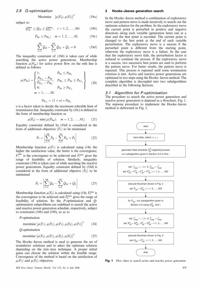
3.1 Algorithm for P-optimisationThe procedure to search the active power generation andreactive power generation is depicted as a flowchart, Fig. 1.The stepwise procedure to implement the Hooke–Jeevesmethod is elaborated in Fig. 2.

generate initial schedule P 0 neglecting losses

run subalgorithm given in Section 3.2 to find �

fix PGi ; run subalgorithm given in

Section 3.3 using Q0Gi , find �

execute flowchart shown in Fig. 2

set PGi = XcGi ; i = 1, 2, …, NG

execute flowchart shown in Fig. 2

set QGi = X cGi ; i = 1, 2, …, NG

stop

input data, select �, �, �

set �cmax = � ; k = 0 �k

max = �cmax

set XcGi = Qk

Gi ; XkGi = Qk

Gi ; i =1, 2, …, NG

start

set �cmax = � ; k = 0 �max = �c

max

set XcGi = P k

Gi ; XkGi = P k

Gi ; i = 1, 2, …, NG

k

Gi

Fig. 1 Flow chart to search active and reactive power generation


3.2 P-optimisation subalgorithmThe stepwise procedure to evaluate the functions relating toP-optimisation problem is as follows:

Decoupled load flow is run.

Compute loss coefficients and active power loss using (11a),(11b) and (9a). Compute active power line flows using (13).

Compute objective function values ð�F1Þ; ð�F2Þ; ð�F3Þ; ð�F7Þusing (4), (6), (7) and (22).

Membership functions mð�F1Þ; mð�F2Þ; mð�F3Þ; mð�F7Þ are evalu-ated using (14) and m �F6ð Þ by (21).

Membership function outcome g is selected as

g ¼ Min mðFjÞ; j ¼ 1; 2; 3; 6; 7� �

3.3 Q-optimisation subalgorithmThe stepwise procedure to evaluate functions relating toQ-optimisation problem is as follows:

Decoupled load flow is run by converting PV buses toPQ buses.

Compute loss coefficients and power losses using(11a)–(11d) and (9a) and (9b). Compute active power-lineflows using (13).

Compute objective function �F4 and �F8 using (8) and (23).

Evaluate membership functions m �F4ð Þ and m �F8ð Þ using (14)and m �F5ð Þ; m �F6ð Þ by (17) and (21).

Membership function outcome g is selected as

g ¼ Min mðFjÞ; j ¼ 4; 5; 6; 8� �

4 Test system and results

The validity of the proposed method is demonstrated on anIEEE five-generator, 25-bus, 35-line power system as shownin Fig. 3 [1]. Noninferior solutions for different generationcombinations are searched, using the Hooke–Jeeves patternsearch method, considering all the objectives simulta-neously. The probability properties are known from thepast history or can be estimated via the Monte Carlosimulation technique [9]. There is a need to use exact valuesof coefficients of variation and correlation coefficientsas and when required. Variance is represented by thecoefficient of variation. The covariance of bivariaterandom variables can be considered positive or negative,

yes

no

yes

yes

no

start

set XGi = XcGi i = 1, 2, …, NG and k = 0

� = � (XG1,.,XGm ,.,XGNG )

�+ = � (XG1,.,XGm +�,.,XGNG )

�− = � (XG1,.,XGm − �,.,XGN )

� max = max (�, �+ , �− )

�max > �cmax?

m < NG ?no

return

�cmax ≤ �k

max

no

�cmax = �max X c

Gm

corresponds to �max

m = m +1

m = 1

yes E F� = � /�

|| � || < ε ?

F

set k = k + 1, pattern move

X (k + 1) = XkGi + (Xk

Gi − X (k − 1));

i = 1, 2, …, NG and find � (k + 1)

� (k + 1) > �k ?

yes

no

E

X cGi = X k

Gi ; i = 1, 2, ..., NG

set � k+1 = �cmax , X (k + 1) = X c

Gi i = 1, 2…NGmax Gi

max

Gi Gi

max max

Fig. 2 Flow chart for Hooke–Jeeves pattern search method

3 67

8 9 10

4

20

17

1615 14

13

2

25 23

11

18 19

21

112

5

24 22

Fig. 3 Line diagram of 25-bus 35-line power system network


represented by correlation coefficients. The correlationcoefficients are generally varied from �1.0 to 1.0. Thepreferred solutions are obtained using the min–maxtechnique, for the following four cases in which diversevalues of coefficients of variation and correlation coeffi-cients are considered:

Case 1: All the coefficients of variance and correlationcoefficients are considered as zero.

Case 2:

CðViÞ ¼ 0:05; CðdiÞ ¼ 0:10; i ¼ 1; 2; . . . ;NB

RðVi; VjÞ¼Rðdi; djÞ¼1:0; i¼1; 2; . . . ;NB;

j ¼ 1; 2; . . . ;NB

Case 3:

CðaiÞ ¼ CðbiÞ ¼ CðdiÞ ¼ CðeiÞ ¼ 0:1;

CðPGiÞ ¼ CðQGiÞ ¼ 0:10; i ¼ 1; 2; . . . ;NG

Rðai; PGiÞ ¼ Rðbi; PGiÞ ¼ Rðdi; PGiÞ ¼ Rðei; PGiÞ ¼ 1:0;

i ¼ 1; 2; . . . ;NG

RðPi; PjÞ ¼ RðQi;QjÞ ¼ RðPi;QjÞ ¼ RðQi; PjÞ ¼ 1:0;

i ¼ 1; 2; . . . ;NB; j ¼ 1; 2; . . . ;NB

Case 4:

CðaiÞ ¼ CðbiÞ ¼ CðdiÞ ¼ CðeiÞ ¼ 0:1;

CðPGiÞ ¼ CðQGiÞ ¼ 0:10; i ¼ 1; 2; . . . ;NG

Rðai; PGiÞ ¼ Rðbi; PGiÞ ¼ Rðdi; PGiÞ ¼ Rðei; PGiÞ ¼ 1:0;

i ¼ 1; 2; . . . ;NG

RðPi; PjÞ ¼ RðQi;QjÞ ¼ RðPi;QjÞ ¼ RðQi; PjÞ ¼ 1:0;

i ¼ 1; 2; . . . ;NB; j ¼ 1; 2; . . . ;NB

CðViÞ ¼ 0:05; CðdiÞ ¼ 0:10; RðVi; VjÞ ¼ Rðdi; djÞ ¼ 1:0;

i ¼ 1; 2; . . . ;NB; j ¼ 1; 2; . . . ;NB

After observing the trend of results, the following minimumand maximum values for the objectives were selected:

�F min1 ¼ 1980:0 $=h; �F max

1 ¼ 2100:0 $=h

�F min2 ¼ 1040:0Kg=h; �F max

2 ¼ 1300:0Kg=h

�F min3 ¼ 0:01 ðp:u:Þ2; �F max

3 ¼ 0:8 ðp:u:Þ2

�F min4 ¼ 0:001 ðp:u:Þ2; �F max

4 ¼ 0:08 ðp:u:Þ2

�F min5 ¼ Vj jmin¼ 0:95; �F max

5 ¼ Vj jmax¼ 1:10

�F min6m¼ PTRm ; �F max

6m¼ 1:5 � PTRm

�F min7 ¼ 0:0001 ðp:u:Þ; �F max

7 ¼ 1:0 ðp:u:Þ�F min8 ¼ 0:0001 ðp:u:Þ; �F max

8 ¼ 1:0 ðp:u:Þ

Table 1: Generation schedule corresponding to optimum solutions for different cases after P-optimisation

Case PG1 (p.u.) PG2 (p.u.) PG3 (p.u.) PG4 (p.u.) PG5 (p.u.)

1 2.366115 0.902641 1.625000 0.658803 1.895422

2 2.471631 0.940141 1.475351 0.658803 1.895422

3 2.506098 0.902641 1.475351 0.658803 1.895422

4 2.394965 0.855766 1.653476 0.621302 1.923544

Min limits 0.5 0.2 0.3 0.1 0.4

Max limits 3.0 1.25 1.75 0.75 2.5

Table 2: Generation schedule corresponding to optimum solutions for different cases after Q-optimisation

Case PG1 (p.u.) QG1 (p.u.) QG2 (p.u.) QG3 (p.u.) QG4 (p.u.) QG5 (p.u.)

1 2.357993 1.054207 0.151648 0.370392 0.393753 �0.157195

2 2.463837 1.031068 0.145733 0.390494 0.388986 �0.161833

3 2.500277 1.115880 �0.144860 0.324249 0.323792 0.174896

4 2.391449 1.247414 0.077152 0.207598 0.403059 �0.091803

Min limits 0.5 �0.25 �0.45 �0.30 �0.50 �0.50

Max limits 3.0 1.5 1.0 1.0 1.0 1.5

Table 3: Objective function values after active and reactive power optimisation

Case Cost of generation �F1, ($/h) Emission of pollutants �F2 (Kg/h) Active power variance �F3 (p.u.)2

P-search Q-search P-search Q-search P-search Q-search

1 1996.226 1994.189 1133.471 1129.318 0.0 0.0

2 1994.706 1992.726 1168.715 1164.532 0.0 0.0

3 2015.465 2013.957 1217.646 1214.371 0.553285 0.552420

4 2015.702 2014.803 1183.639 1181.756 0.554884 0.554360


5 Results and discussion

System data of a power system network may be subjected todifferent kinds of variations or randomness like errors,inaccuracies and uncertainties while representing differentcharacteristics of the network. These variations aremodelled mathematically in the form of coefficients of

variance and covariance. In the paper four cases have beenconsidered by taking different combinations of coefficientsof variation and covariation of the various randomparameters: fuel cost coefficients, gaseous emission coeffi-cients, active and reactive power injections and hencegenerations, voltage magnitudes and their angles. Thestochastic multiobjective problem is decoupled into two

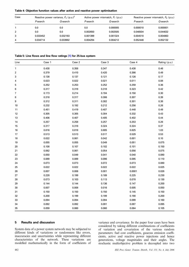
Table 4: Objective function values after active and reactive power optimisation

Case Reactive power variance, �F4 (p.u.)2 Active power mismatch, �F7 (p.u.) Reactive power mismatch, �F8 (p.u.)

P-search Q-search P-search Q-search P-search Q-search

1 0.0 0.0 0.0 0.000005 0.000010 0.000001

2 0.0 0.0 0.002650 0.002505 0.046504 0.044632

3 0.033452 0.032183 0.001399 0.001324 0.004510 0.004863

4 0.034714 0.033982 0.004294 0.004212 0.052446 0.052132

Table 5: Line flows and line flow ratings [1] for 25-bus system

Line Case 1 Case 2 Case 3 Case 4 Rating (p.u.)

1 0.430 0.358 0.347 0.438 0.46

2 0.379 0.410 0.420 0.386 0.49

3 0.138 0.137 0.121 0.126 0.17

4 0.023 0.022 0.021 0.011 0.08

5 0.252 0.253 0.252 0.259 0.36

6 0.317 0.318 0.318 0.323 0.42

7 0.173 0.214 0.194 0.150 0.30

8 0.318 0.317 0.306 0.307 0.39

9 0.312 0.311 0.302 0.301 0.38

10 0.232 0.192 0.212 0.256 0.26

11 0.451 0.419 0.407 0.448 0.49

12 0.305 0.305 0.304 0.332 0.43

13 0.406 0.407 0.405 0.402 0.44

14 0.257 0.258 0.257 0.253 0.26

15 0.317 0.318 0.324 0.324 0.37

16 0.816 0.818 0.805 0.825 1.03

17 0.513 0.513 0.517 0.529 0.53

18 0.022 0.061 0.042 0.001 0.10

19 0.055 0.055 0.049 0.051 0.075

20 0.108 0.107 0.102 0.101 0.150

21 0.062 0.061 0.054 0.056 0.075

22 0.050 0.049 0.041 0.040 0.080

23 0.089 0.089 0.096 0.095 0.110

24 0.073 0.073 0.072 0.073 0.080

25 0.022 0.022 0.022 0.022 0.025

26 0.007 0.006 0.001 0.0001 0.026

27 0.228 0.199 0.189 0.225 0.230

28 0.073 0.103 0.113 0.078 0.130

29 0.144 0.144 0.136 0.147 0.200

30 0.007 0.008 0.016 0.005 0.050

31 0.150 0.150 0.150 0.145 0.150

32 0.200 0.199 0.199 0.190 0.200

33 0.094 0.094 0.094 0.099 0.160

34 0.092 0.092 0.091 0.087 0.095

35 0.059 0.060 0.060 0.064 0.105


deterministic subproblems and solved using the Hooke–Jeeves search technique.

First active power generations are optimised within lowerand upper limits [1] of active power generations ofgenerators to optimise those objectives which are dependenton active power like cost, emission, variance of activepower, active power flow on lines and mismatch of activepower generation to meet its load demand and transmissionlosses. An optimised set of active power generations isobtained along with a set of reactive power generations.Then by taking these generations as the starting or basevalues, reactive power generations are searched by convert-ing PV buses to PQ buses within minimum and maximumcapacity limits of reactive power generations [1]. Objectivesconsidered are variance of reactive power, magnitude ofvoltages at the buses and mismatch of reactive power withits load demand plus losses and also the active power flowon transmission lines to maintain the line security. If linesecurity is not taken into account while searching theschedule of reactive power generation, then active powerflow on some lines may go beyond the limits.

Optimised generation schedules are different for differentcases, thus indicating the need for rescheduling ofgenerators for different variations of parameters. Table 1shows the optimum generation schedules after active powergeneration search and Table 2 depicts the optimumgeneration schedules after reactive power generation search.While optimising the reactive power it is observed thatactive power generation injected at slack bus (G1) getsreduced (comparing columns of Tables 1 and 2 depictingPG1) during load-flow run, therefore cost, emission, active

power variance and power mismatch also get reduced(comparing Q-search columns with P-search columns foreach of the objective function values given in Tables 3 and4) besides optimising reactive power variance and mismatchand voltage profile at the buses. From Table 3 it is observedthat cost and emission are affected more by variations andcovariations in active power generations and in character-istic coefficients of generators, as is evident if case 3 iscompared with case 1. Cost and emission are comparativelyless affected by variations and covariations in bus voltagemagnitudes and their phase angles, as found by comparingcase 2 with case 1 and by comparing case 4 with case 3.From Table 4 it is observed that active and reactive powermismatch is affected more by variations and covariations inbus voltage magnitudes and their angles (cases 2 and 4) thanby variations in power generations and covariations inpower injections (case 3) at the buses.

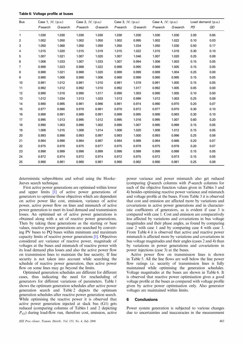
Active power flow on transmission lines is shownin Table 5. All the line flows are well below the line powerflow ratings i.e. security of transmission lines is fullymaintained while optimising the generation schedules.Voltage magnitudes at the buses are shown in Table 6. Itis observed that reactive power optimisation gives a goodvoltage profile at the buses as compared with voltage profilegiven by active power optimisation only. Also generatorvoltages are maintained within limits.

6 Conclusions

Power system generation is subjected to various changesdue to uncertainties and inaccuracies in the measurement

Table 6: Voltage profile at buses

Bus Case 1, 7V7 (p.u.) Case 2, 7V7 (p.u.) Case 3, 7V7 (p.u.) Case 4, 7V7 (p.u.) Load demand (p.u.)

P-search Q-search P-search Q-search P-search Q-search P-search Q-search PD QD

1 1.030 1.030 1.030 1.030 1.030 1.030 1.030 1.030 2.00 0.65

2 1.002 1.050 1.002 1.050 1.002 0.995 1.002 1.022 0.10 0.03

3 1.050 1.060 1.050 1.059 1.050 1.034 1.050 1.030 0.50 0.17

4 1.015 1.020 1.015 1.019 1.015 1.022 1.015 1.018 0.30 0.10

5 1.007 1.021 1.007 1.020 1.007 1.046 1.007 1.020 0.25 0.08

6 1.006 1.033 1.007 1.033 1.007 0.994 1.006 1.003 0.15 0.05

7 0.988 1.023 0.988 1.022 0.988 0.995 0.988 1.005 0.15 0.05

8 0.988 1.021 0.988 1.020 0.989 0.999 0.989 1.004 0.25 0.00

9 0.980 1.008 0.980 1.006 0.980 0.998 0.980 0.995 0.15 0.05

10 0.991 1.012 0.991 1.010 0.991 1.019 0.991 1.005 0.15 0.05

11 0.992 1.012 0.992 1.010 0.992 1.017 0.992 1.005 0.05 0.00

12 0.990 1.018 0.990 1.017 0.990 1.003 0.990 1.005 0.10 0.00

13 1.012 1.034 1.013 1.033 1.013 0.999 1.012 1.003 0.25 0.08

14 0.980 0.985 0.981 0.986 0.981 0.974 0.980 0.970 0.20 0.07

15 0.977 0.980 0.978 0.981 0.978 0.972 0.977 0.970 0.30 0.10

16 0.988 0.991 0.989 0.991 0.989 0.985 0.988 0.983 0.30 0.10

17 0.995 1.013 0.995 1.012 0.995 1.016 0.995 1.007 0.60 0.20

18 0.990 1.003 0.990 1.002 0.990 1.007 0.990 0.999 0.15 0.05

19 1.008 1.015 1.008 1.014 1.008 1.020 1.008 1.012 0.15 0.05

20 0.993 0.998 0.993 0.997 0.993 1.000 0.993 0.996 0.25 0.08

21 0.984 0.998 0.984 0.987 0.984 0.989 0.984 0.986 0.20 0.07

22 0.975 0.978 0.975 0.977 0.975 0.979 0.975 0.976 0.20 0.07

23 0.998 0.999 0.998 0.999 0.998 0.999 0.998 0.998 0.15 0.05

24 0.972 0.974 0.972 0.974 0.972 0.975 0.972 0.973 0.15 0.05

25 0.980 0.981 0.980 0.981 0.980 0.982 0.980 0.981 0.25 0.08


and forecasting of various parameters of the network. Totake these variations into account a stochastic multi-objective problem has been undertaken and random natureof various parameters has been considered by coefficients ofvariance and covariance of parameters. The expected valuesof various objective functions are calculated instead ofdeterministic ones. It is clear from the results thatgenerations need rescheduling if system parameters vary.The Hooke–Jeeves pattern-search method has been used tosearch the optimum active power generation schedule tosolve the stochastic multiobjective problem. Constraints aretaken as the additional objectives to be optimised. Themethod used for solving multiobjective problem of alloca-tion of active and reactive power generations to generatorsis very simple and straightforward. No tedious derivationsof the objective functions are required to be calculated, sothe technique is equally good for discontinuous functions.Convergence of solution is ensured. The optimum resultobtained is sensitive to the starting values of the generationschedule and step factor taken in the exploratory move, butit is not very difficult to select proper values for them by anexpert decision maker. In such a case the solution procedurewill take more iterations.

7 References

1 Hota, P.K., Chakrabarti, R., and Chatopadhyay, P.K.:‘Economic emission load dispatch through an interactivefuzzy satisfying method’, Electr. Power Syst. Res., 2000, 54,pp. 151–157

2 Brar, Y.S., Dhillon, J.S., and Kothari, D.P.: ‘Multiobjective loaddispatch by fuzzy logic based searching weightage pattern’, Electr.Power Syst. Res., 2002, 63, pp. 149–160

3 Dhillon, J.S., Parti, S.C., and Kothari, D.P.: ‘Stochastic economicemission load dispatch’, Electr. Power Syst. Res., 1993, 26,pp. 179–186

4 Chang, C.S., and Fu,W.: ‘Stochastic multiobjective generation dispatchof combined heat and power systems’, IEE Proc-Gener. Transm.Distrib., 1998, 145, (5), pp. 583–591

5 Arya, L.D., Choube, S.C., and Kothari, D.P.: ‘A nondecomposedapproach for security constrained economic dispatch’, J. Inst. Eng.(India), 1997, 77, pp. 229–234

6 Arya, L.D., Choube, S.C., and Kothari, D.P.: ‘Reactive poweroptimization using static voltage stability index’, Electr. PowerComponen. Syst., 2001, 29, pp. 615–628

7 Bijwe, P.R., Kothari, D.P., and Arya, L.D.: ‘Alleviation of lineoverloads and voltage violations by corrective rescheduling’, IEE Proc.-C, 1993, 140, (4), pp. 249–255

8 Arya, L.D., Choube, S.C., and Kothari, D.P.: ‘Line outage ranking forvoltage limit violations with corrective rescheduling avoiding masking’,Electr. Power Energy Syst., 2001, 23, pp. 837–846

9 Dhillon, J.S., Parti, S.C., and Kothari, D.P.: ‘Fuzzy decision makingin stochastic multiobjective short-term hydrothermal scheduling’, IEEProc.-C, 2002, 149, (2), pp. 191–200


stochastic multiobjective generation allocation using pattern-search method

Documents