stochastic layered alpha blending - cwyman.org
TRANSCRIPT

Chris Wyman
STOCHASTIC LAYERED ALPHA
BLENDING
SIGGRAPH 2016; July 26, 2016; Anaheim, CA

2
TRANSPARENCY IS HARD
Work fits in the context of “order independent transparency”
In real time, transparency is hard

3
TRANSPARENCY IS HARD
Work fits in the context of “order independent transparency”
In real time, transparency is hard
Why? Existing algorithms:
Not in same rendering pass as opaque
Interacts in complex ways with other effects (e.g., AA)
(Some) greedily use memory
Often use complex locking and atomics

4
TRANSPARENCY IS HARD
Work fits in the context of “order independent transparency”
In real time, transparency is hard
Why? Existing algorithms:
Not in same rendering pass as opaque
Interacts in complex ways with other effects (e.g., AA)
(Some) greedily use memory
Often use complex locking and atomics
Takeaway:
Current solutions not ideal; many minimize use of transparency

5
WHAT’S THE PROBLEM?[Porter and Duff 84] outlined numerous common compositing operations
The “over” operator, using multiplicative blending, describes most real interactions:
For streaming compute, you need to sort geometry or keep all αi and ci around
Incorrect Order Correct Order
Merge two fragments then later try to insert one in between?

6
WHAT’S THE PROBLEM?Sorting geometry in advance can fail
May be no “correct” order for triangles
Keep a list of fragments per pixel (i.e., A-Buffers [Carpenter 84])
Virtually unbounded** GPU memory
Still need to sort fragments to apply over operator in correctly
Not just a raster problem; affects ray tracing, too
Unless it guarantees ray hits returned perfectly ordered
** You can define a very conservative upper bound, but it’s quite unhelpful.

7
RECENT WORK: OIT CONTINUUM * See my High Performance Graphics 2016 paper

8
Interesting note
RECENT WORK: OIT CONTINUUM * See my High Performance Graphics 2016 paper

9
So what is Stochastic Layered Alpha Blending?

10
WHAT IS STOCHASTIC LAYERED ALPHA BLEND
Shows how to use stochasm in a k-buffer algorithm
I.e., allows stochastic insertion of fragments

11
WHAT IS STOCHASTIC LAYERED ALPHA BLEND
Shows how to use stochasm in a k-buffer algorithm
I.e., allows stochastic insertion of fragments
Shows stochastic transparency ≡ k-buffering

12
WHAT IS STOCHASTIC LAYERED ALPHA BLEND
Shows how to use stochasm in a k-buffer algorithm
I.e., allows stochastic insertion of fragments
Shows stochastic transparency ≡ k-buffering
How?
By providing an explicit parameter that transitions
Stochastic transparency [Enderton 10] ↔ hybrid transparency [Maule 13]
Stochastic transparency
HybridtransparencyContinuous knob transitioning between these techniques

13
To Understand:Start With Stochastic Transparency

14
WHAT IS STOCHASTIC TRANSPARENCY?
When rasterizing frag into k-sample buffer:
Stochastically cover α • k samples

15
WHAT IS STOCHASTIC TRANSPARENCY?
When rasterizing frag into k-sample buffer:
Stochastically cover α • k samples
Let’s look at an example pixel with 16x MSAA
(MSAA pattern simplified for display)
1.0 1.0 1.0 1.0
1.0 1.0 1.0 1.0
1.0 1.0 1.0 1.0
1.0 1.0 1.0 1.0
Values represent current depth sample

16
WHAT IS STOCHASTIC TRANSPARENCY?
When rasterizing frag into k-sample buffer:
Stochastically cover α • k samples
Let’s look at an example pixel with 16x MSAA
(MSAA pattern simplified for display)
First: draw red fragment, z = 0.5, α = 0.5
0.5 1.0 1.0 0.5
1.0 0.5 0.5 1.0
0.5 1.0 0.5 0.5
1.0 0.5 1.0 1.0
Values represent current depth sample
Set 8 samples to red; depth test each

17
WHAT IS STOCHASTIC TRANSPARENCY?
When rasterizing frag into k-sample buffer:
Stochastically cover α • k samples
Let’s look at an example pixel with 16x MSAA
(MSAA pattern simplified for display)
First: draw red fragment, z = 0.5, α = 0.5
Second: draw blue fragment, z = 0.7, α = 0.5
0.5 1.0 0.7 0.5
0.7 0.5 0.5 0.7
0.5 0.7 0.5 0.5
1.0 0.5 0.7 1.0
Values represent current depth sample
Set 8 samples to blue; depth test each

18
WHAT IS STOCHASTIC TRANSPARENCY?
When rasterizing frag into k-sample buffer:
Stochastically cover α • k samples
Let’s look at an example pixel with 16x MSAA
(MSAA pattern simplified for display)
First: draw red fragment, z = 0.5, α = 0.5
Second: draw blue fragment, z = 0.7, α = 0.5
Third: draw green fragment, z = 0.3, α = 0.5
0.5 0.3 0.7 0.3
0.7 0.5 0.5 0.3
0.5 0.3 0.3 0.5
0.3 0.3 0.7 0.3
Values represent current depth sample
Set 8 samples to green; depth test each

19
WHAT IS STOCHASTIC TRANSPARENCY?
When rasterizing frag into k-sample buffer:
Stochastically cover α • k samples
Let’s look at an example pixel with 16x MSAA
(MSAA pattern simplified for display)
First: draw red fragment, z = 0.5, α = 0.5
Second: draw blue fragment, z = 0.7, α = 0.5
Third: draw green fragment, z = 0.3, α = 0.5
Fourth: draw yellow fragment, z = 0.9, α = 1.0
0.5 0.3 0.7 0.3
0.7 0.5 0.5 0.3
0.5 0.3 0.3 0.5
0.3 0.3 0.7 0.3
Values represent current depth sample
Set 16 samples to yellow; depth test each

20
WHAT IS STOCHASTIC TRANSPARENCY?
When rasterizing frag into k-sample buffer:
Stochastically cover α • k samples
Let’s look at an example pixel with 16x MSAA
(MSAA pattern simplified for display)
First: draw red fragment, z = 0.5, α = 0.5
Second: draw blue fragment, z = 0.7, α = 0.5
Third: draw green fragment, z = 0.3, α = 0.5
Fourth: draw yellow fragment, z = 0.9, α = 1.0
2nd pass accum. color using this as depth oracle
0.5 0.3 0.7 0.3
0.7 0.5 0.5 0.3
0.5 0.3 0.3 0.5
0.3 0.3 0.7 0.3
Values represent current depth sample

21
OBSERVATIONS
Can lose surfaces (like yellow one)
But it still converges; surface loss is stochastic
0.5 0.3 0.7 0.3
0.7 0.5 0.5 0.3
0.5 0.3 0.3 0.5
0.3 0.3 0.7 0.3

22
OBSERVATIONS
Can lose surfaces (like yellow one)
But it still converges; surface loss is stochastic
Loss worse if nearby surfaces almost opaque
Could easily lose blue surface
0.5 0.3 0.7 0.3
0.7 0.5 0.5 0.3
0.5 0.3 0.3 0.5
0.3 0.3 0.7 0.3

23
OBSERVATIONS
Can lose surfaces (like yellow one)
But it still converges; surface loss is stochastic
Loss worse if nearby surfaces almost opaque
Could easily lose blue surface
Also noticed in my experiments
Dashboard and seat noisier with high alpha than low!
α = 0.4, 8 spp
α = 0.98, 8 spp
Note: Even uses stratified sampling!

24
OBSERVATIONS
Can lose surfaces (like yellow one)
But it still converges; surface loss is stochastic
Loss worse if nearby surfaces almost opaque
Could easily lose blue surface
Also noticed in my experiments
Dashboard and seat noisier with high alpha than low!
Seems wasteful to store 8 copies of z = 0.3 **
Why not store one copy of z = 0.3 and a coverage mask?
0.5 0.3 0.7 0.3
0.7 0.5 0.5 0.3
0.5 0.3 0.3 0.5
0.3 0.3 0.7 0.3
** Glossing over some details here; feel free to ask later.

25
OBSERVATIONS
Can lose surfaces (like yellow one)
But it still converges; surface loss is stochastic
Loss worse if nearby surfaces almost opaque
Could easily lose blue surface
Also noticed in my experiments
Dashboard and seat noisier with high alpha than low!
Seems wasteful to store 8 copies of z = 0.3 **
Why not store one copy of z = 0.3 and a coverage mask?
Implicitly layered − stores (up to) 16 surfaces per pixel (for 16x MSAA)
Also wasteful to store just 3 layers in a structure that can hold 16
0.5 0.3 0.7 0.3
0.7 0.5 0.5 0.3
0.5 0.3 0.3 0.5
0.3 0.3 0.7 0.3

26
Stochastic Layered Alpha Blending (SLAB)

27
WHAT IS STOCHASTIC LAYERED ALPHA BLEND?
An explicit k-layered algorithm with stoc. transparency’s characteristics

28
WHAT IS STOCHASTIC LAYERED ALPHA BLEND?
An explicit k-layered algorithm with stoc. transparency’s characteristics
Memory: store k layers, each with depth and b-bit coverage mask
Insertion: probabilistically insert fragments into per-pixel lists
Merging: if > k layers, simply discard the furthest

29
WHAT IS STOCHASTIC LAYERED ALPHA BLEND?
An explicit k-layered algorithm with stoc. transparency’s characteristics
Memory: store k layers, each with depth and b-bit coverage mask
Insertion: probabilistically insert fragments into per-pixel lists
Merging: if > k layers, simply discard the furthest
Identical results to k spp stoc. transparency, if k ≥ b
But can independently change values of k and b

30
WHAT IS STOCHASTIC LAYERED ALPHA BLEND?
An explicit k-layered algorithm with stoc. transparency’s characteristics
Memory: store k layers, each with depth and b-bit coverage mask
Insertion: probabilistically insert fragments into per-pixel lists
Merging: if > k layers, simply discard the furthest
Identical results to k spp stoc. transparency, if k ≥ b
But can independently change values of k and b
Useful since stoc. transp. rarely stores k surfaces in a k-sample buffer
Also can explicitly increase b much further → reduce noise on existing layers

31
WHAT IS STOCHASTIC LAYERED ALPHA BLEND?
Our same example from before:
First: draw red fragment, z = 0.5, α = 0.5
Coverage Mask Depth
0.5
La
ye
rs

32
WHAT IS STOCHASTIC LAYERED ALPHA BLEND?
Our same example from before:
First: draw red fragment, z = 0.5, α = 0.5
Second: draw blue fragment, z = 0.7, α = 0.5
Coverage Mask Depth
0.5
0.7
La
ye
rs

33
WHAT IS STOCHASTIC LAYERED ALPHA BLEND?
Our same example from before:
First: draw red fragment, z = 0.5, α = 0.5
Second: draw blue fragment, z = 0.7, α = 0.5
Third: draw green fragment, z = 0.3, α = 0.5
Coverage Mask Depth
0.3
0.5
0.7
La
ye
rs

34
WHAT IS STOCHASTIC LAYERED ALPHA BLEND?
Our same example from before:
First: draw red fragment, z = 0.5, α = 0.5
Second: draw blue fragment, z = 0.7, α = 0.5
Third: draw green fragment, z = 0.3, α = 0.5
Fourth: draw yellow fragment, z = 0.9, α = 1.0
Coverage Mask Depth
0.3
0.5
0.7
0.9
La
ye
rs

35
WHAT IS STOCHASTIC LAYERED ALPHA BLEND?
Our same example from before:
First: draw red fragment, z = 0.5, α = 0.5
Second: draw blue fragment, z = 0.7, α = 0.5
Third: draw green fragment, z = 0.3, α = 0.5
Fourth: draw yellow fragment, z = 0.9, α = 1.0
Layers get inserted only if not occluded
Adds stochasm, if masks randomly chosen
Different random masks might keep this layer
Coverage Mask Depth
0.3
0.5
0.7
0.9
La
ye
rs

36
WHAT IS STOCHASTIC LAYERED ALPHA BLEND?
Our same example from before:
First: draw red fragment, z = 0.5, α = 0.5
Second: draw blue fragment, z = 0.7, α = 0.5
Third: draw green fragment, z = 0.3, α = 0.5
Fourth: draw yellow fragment, z = 0.9, α = 1.0
Layers get inserted only if not occluded
Adds stochasm, if masks randomly chosen
Different random masks might keep this layer
If k = 2, layers beyond 2nd get discarded
Coverage Mask Depth
0.3
0.5
0.7
0.9
La
ye
rs

37
ADJUSTING PARAMETERS
Aim to reduce noise
One way: avoid discarding layers that impact color
Coverage Mask Depth
0.3
0.5
0.7
0.9
La
ye
rs

38
ADJUSTING PARAMETERS
Aim to reduce noise
One way: avoid discarding layers that impact color
How to increase chance to store yellow frag?
Coverage Mask Depth
0.3
0.5
0.7
0.9
La
ye
rs

39
ADJUSTING PARAMETERS
Aim to reduce noise
One way: avoid discarding layers that impact color
How to increase chance to store yellow frag?
Increase number of bits in coverage mask
Coverage Mask Depth
0.3
0.5
0.7
0.9
La
ye
rs

40
ADJUSTING PARAMETERS
Aim to reduce noise
One way: avoid discarding layers that impact color
How to increase chance to store yellow frag?
Increase number of bits in coverage mask
Larger coverage masks → lower noise
What happens as # coverage bits increases?
Coverage Mask Depth
0.3
0.5
0.7
0.9
La
ye
rs

41
ADJUSTING PARAMETERS
Aim to reduce noise
One way: avoid discarding layers that impact color
How to increase chance to store yellow frag?
Increase number of bits in coverage mask
Larger coverage masks → lower noise
What happens as # coverage bits increases?
Starts to behave as alpha
Interesting to ask:
Can we stochastically insert fragments using alpha?
Coverage Mask Depth
0.3
0.5
0.7
0.9
La
ye
rs

42
SLAB USING IMPLICIT COVERAGE
Let’s compute an insertion probability
Q: What’s the chance random bitmask B is visible behind random bitmask A?
Bitmask A Bitmask B0 Bitmask B1
Visible Hidden

43
SLAB USING IMPLICIT COVERAGE
Let’s compute an insertion probability
Q: What’s the chance random bitmask B is visible behind random bitmask A?
Bitmask A Bitmask B0
Hidden if none of these getcovered by bits in bitmask B

44
SLAB USING IMPLICIT COVERAGE
Let’s compute an insertion probability
Q: What’s the chance random bitmask B is visible behind random bitmask A?
Bitmask A Bitmask B0
Naïve random sampling:
Covered with probability αB
Uncovered with prob (1 – αB)

45
SLAB USING IMPLICIT COVERAGE
Let’s compute an insertion probability
Q: What’s the chance random bitmask B is visible behind random bitmask A?
Bitmask A Bitmask B0
All uncovered with prob: (1–αB)6
Bitmask B visible with prob: 1-(1–αB)6
Naïve random sampling:
Covered with probability αB
Uncovered with prob (1 – αB)

46
SLAB USING IMPLICIT COVERAGE
Let’s compute an insertion probability
Q: What’s the chance random bitmask B is visible behind random bitmask A?
𝑃𝑏 𝛽𝐴, 𝛽𝐵 = 1 − 1 −𝛽𝐵𝑏
(𝑏−𝛽𝐴)
Or
𝑃𝑏 𝛽𝐴, 𝛼𝐵 = 1 − 1 − 𝛼𝐵(𝑏−𝛽𝐴)
Bitmask A
𝛽A ≡ # bits covered
𝛽A= 𝛼A𝑏 or 𝛼A𝑏
for b bits in bitmask

47
SLAB USING IMPLICIT COVERAGE
Let’s compute an insertion probability
Q: What’s the chance random bitmask B is visible behind random bitmask A?
𝑃𝑏 𝛽𝐴, 𝛽𝐵 = 1 − 1 −𝛽𝐵𝑏
(𝑏−𝛽𝐴)
Or
𝑃𝑏 𝛽𝐴, 𝛼𝐵 = 1 − 1 − 𝛼𝐵(𝑏−𝛽𝐴)
Bitmask A
𝛽A ≡ # bits covered
𝛽A= 𝛼A𝑏 or 𝛼A𝑏
for b bits in bitmask
prob of leaving1 bit uncovered
number of bits that must be uncovered

48
SLAB USING IMPLICIT COVERAGE
Let’s compute an insertion probability
Q: How about for random masks using stratified samples?
𝑃𝑏 𝛽𝐴, 𝛽𝐵 = 1 −
𝛽𝐴! 𝑏−𝛽𝐵 !
𝑏! 𝛽𝐴−𝛽𝐵 !if 𝛽𝐵 ≤ 𝛽𝐴
1 if 𝛽𝐵 > 𝛽𝐴
Bitmask A
𝛽A ≡ # bits covered
Based on combinatorics
Choosing dependent probabilities so all mask bits in B are covered by A

49
WAIT! NOT USING INFINITE # BITS?
Both equations require a number of bits b in the coverage mask
𝑃𝑏 𝛽𝐴, 𝛽𝐵 = 1 −
𝛽𝐴! 𝑏−𝛽𝐵 !
𝑏! 𝛽𝐴−𝛽𝐵 !if 𝛽𝐵 ≤ 𝛽𝐴
1 if 𝛽𝐵 > 𝛽𝐴using stratified random samples
𝑃𝑏 𝛽𝐴, 𝛽𝐵 = 1 − 1 −𝛽𝐵
𝑏
(𝑏−𝛽𝐴)using naïve random samples

50
WAIT! NOT USING INFINITE # BITS?
Both equations require a number of bits b in the coverage mask
Can ask what happens to Pb as b → ∞
Turns out as b → ∞, Pb → 1
Instead of stochastic insertion of fragments, they’re always inserted
𝑃𝑏 𝛽𝐴, 𝛽𝐵 = 1 −
𝛽𝐴! 𝑏−𝛽𝐵 !
𝑏! 𝛽𝐴−𝛽𝐵 !if 𝛽𝐵 ≤ 𝛽𝐴
1 if 𝛽𝐵 > 𝛽𝐴using stratified random samples
𝑃𝑏 𝛽𝐴, 𝛽𝐵 = 1 − 1 −𝛽𝐵
𝑏
(𝑏−𝛽𝐴)using naïve random samples

51
WAIT! NOT USING INFINITE # BITS?
Both equations require a number of bits b in the coverage mask
Can ask what happens to Pb as b → ∞
Turns out as b → ∞, Pb → 1
Instead of stochastic insertion of fragments, they’re always inserted
Going back to our continuum
When b = k, SLAB is equivalent to stochastic transparency
When b → ∞, SLAB is equivalent to hybrid transparency (a variant of k-buffer)

52
WAIT! NOT USING INFINITE # BITS?
To get something between k-buffers and stoc. transp.
Need to use k ≤ b < ∞

53
WAIT! NOT USING INFINITE # BITS?
To get something between k-buffers and stoc. transp.
Need to use k ≤ b < ∞
Can do this with an explicit coverage mask with b random bits
Using deterministic insertion based on random coverage masks

54
WAIT! NOT USING INFINITE # BITS?
To get something between k-buffers and stoc. transp.
Need to use k ≤ b < ∞
Can do this with an explicit coverage mask with b random bits
Using deterministic insertion based on random coverage masks
Can do this with an implicit coverage (i.e., alpha) using b virtual bits
Using stochastic insertion using probability functions
b only controls distance along the k-buffer ↔ stoc transp continuum

55
Let’s demonstrate

56
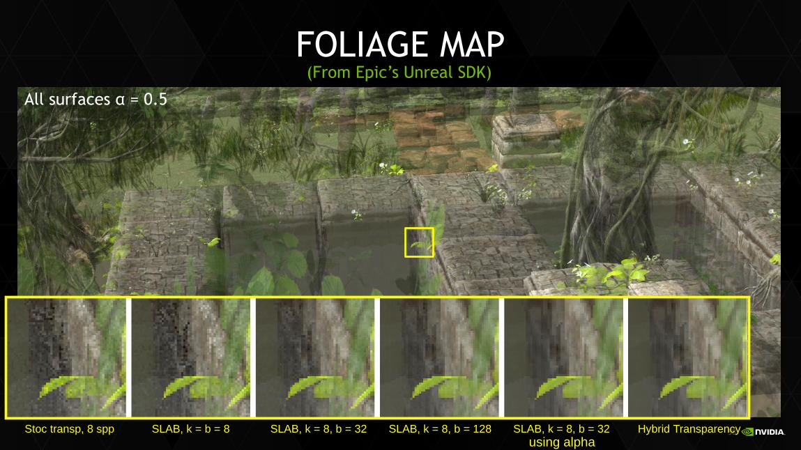
FOLIAGE MAP
All surfaces α = 0.5
(From Epic’s Unreal SDK)

57
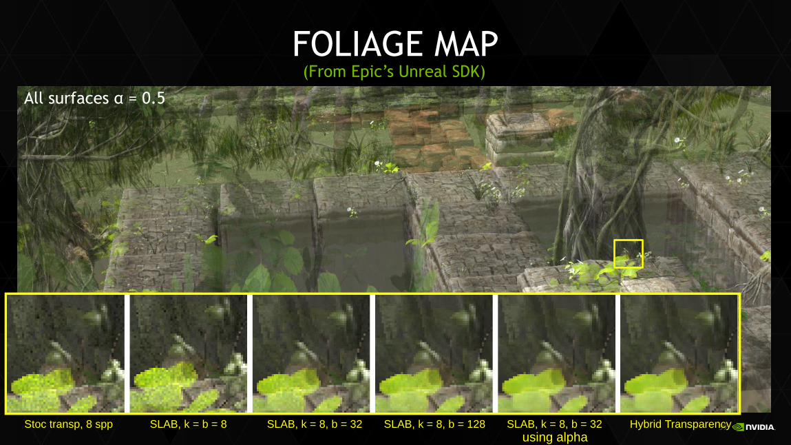
FOLIAGE MAP
All surfaces α = 0.5
Stoc transp, 8 spp SLAB, k = b = 8 SLAB, k = 8, b = 32 SLAB, k = 8, b = 128 SLAB, k = 8, b = 32 Hybrid Transparency
using alpha
(From Epic’s Unreal SDK)
58
FOLIAGE MAP
All surfaces α = 0.5
Stoc transp, 8 spp SLAB, k = b = 8 SLAB, k = 8, b = 32 SLAB, k = 8, b = 128 SLAB, k = 8, b = 32 Hybrid Transparency
using alpha
(From Epic’s Unreal SDK)
59
FOLIAGE MAP
All surfaces α = 0.5
Stoc transp, 8 spp SLAB, k = b = 8 SLAB, k = 8, b = 32 SLAB, k = 8, b = 128 SLAB, k = 8, b = 32 Hybrid Transparency
using alpha
(From Epic’s Unreal SDK)

60
STOCHASTIC TRANSPARENCY TO K-BUFFERS
Stochastic Layered Alpha Blending, k=b=4 Stochastic Transparency, 4 spp

61
STOCHASTIC TRANSPARENCY TO K-BUFFERS
Stochastic Layered Alpha Blending, k=4, b=32 Stochastic Transparency, 4 spp

62
STOCHASTIC TRANSPARENCY TO K-BUFFERS
Stochastic Layered Alpha Blending, k=4, b=8(using alpha rather than coverage)
Stochastic Transparency, 4 spp
63
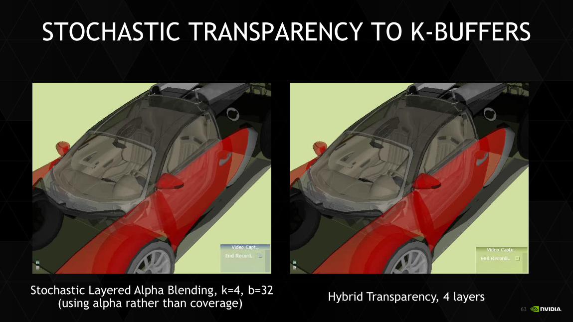
STOCHASTIC TRANSPARENCY TO K-BUFFERS
Stochastic Layered Alpha Blending, k=4, b=32(using alpha rather than coverage)
Hybrid Transparency, 4 layers

64
Summary
65
SUMMARY
Proposed new algorithm
Stochastic layered alpha blending (SLAB)

66
SUMMARY
Proposed new algorithm
Stochastic layered alpha blending (SLAB)
Key takeaways:
K-buffers need not be deterministic
Stochastic transparency and k-buffering are similar; transition via bit count
“Stochastic” need not mean random bitmask generation
Algorithms connecting others useful; here, allow trading noise for bias
SLAB with alpha values can stratify samples in z (between layers)
(Not really discussed in this talk)

67
QUESTIONS?E-mail: [email protected]: @_cwyman_
Stochastic transparency
4 spp
SLAB k = 4, b = 4
Hybridtransparency
4 layers
SLAB k = 4, b = 16using alpha
Multi-layeralpha blending
4 layers
Ground truth(A-buffer)
Blacksmith building, from Unity’s “The Blacksmith” demo
Paper PDF: