stochastic last-mile delivery with crowd-shipping and ...about crowd-shippers and delivery tasks is...

Stochastic Last-mile Delivery with Crowd-shippingand Mobile Depots

Kianoush MousaviDepartment of Civil and Mineral Engineering, University of Toronto, Toronto, Ontario M5S 1A4, Canada,

[email protected]

Merve BodurDepartment of Mechanical and Industrial Engineering, University of Toronto, Toronto, Ontario M5S 3G8, Canada,

[email protected]

Matthew J. RoordaDepartment of Civil and Mineral Engineering, University of Toronto, Toronto, Ontario M5S 1A4, Canada,

[email protected]

This paper proposes a two-tier last-mile delivery model that optimally selects mobile depot locations in

advance of full information about the availability of crowd-shippers, and then transfers packages to crowd-

shippers for the final shipment to the customers. Uncertainty in crowd-shipper availability is incorporated

by modeling the problem as a two-stage stochastic integer program. Enhanced decomposition solution algo-

rithms including branch-and-cut and cut-and-project frameworks are developed. A risk-averse approach is

compared against a risk-neutral approach by assessing conditional-value-at-risk. A detailed computational

study based on the City of Toronto is conducted. The deterministic version of the model outperforms a

capacitated vehicle routing problem on average by 20%. For the stochastic model, decomposition algorithms

usually discover near-optimal solutions within two hours for instances up to a size of 30 mobile depot loca-

tions, 40 customers and 120 crowd-shippers. The cut-and-project approach outperforms the branch-and-cut

approach up to 85% in the risk-averse setting in certain instances. The stochastic model provides solutions

that are 3.35% to 6.08% better than the deterministic model, and the improvements are magnified with the

increased uncertainty in crowd-shipper availability. A risk-averse approach leads the operator to send more

mobile depots or postpone customer deliveries, to reduce the risk of high penalties for non-delivery.

Key words : Last-mile delivery, crowd-shipping, mobile depot, two-stage stochastic integer programming,

decomposition, value of stochastic solution, conditional-value-at-risk

1. Introduction

Innovative and cost-effective last-mile delivery solutions are needed in response to the boom in

e-commerce and the growing demand for fast home deliveries. The global last-mile delivery market

value is expected to grow from 1.99 Billion USD to 7.69 Billion USD by 2026 driven by an upsurge

of e-commerce and expectation for faster delivery times by customers (Insight Partners 2019). In

Canada, 48 percent of e-shoppers reside in urban areas resulting in high density of demand for last

1

2

mile delivery (Lee, Kim, and Wiginton 2019). This has led to an increase of business-to-consumer

related commercial vehicle movements in already congested urban road networks. Truck movements

in urban areas are notorious for slowing down traffic, parking illegally and causing air pollution

and noise. For instance, in 2012, commercial vehicles received 66 percent of all parking tickets in

downtown Toronto, Canada (Rosenfield et al. 2016). Reducing urban truck traffic would diminish

some of the negative externalities in dense urban areas.

In response to these issues, urban consolidation centres have been established in some cities to

increase consolidation of goods and decrease truck travel on urban road networks (Van Rooijen

and Quak 2010). However, large public subsidy and high costs of establishing and operating urban

consolidation centres make them unsustainable in some cases (Lin, Chen, and Kawamura 2016,

Van Duin et al. 2016). Mobile depots have been proposed as a more cost-effective and flexible

alternative. Verlinde et al. (2014) defined a mobile depot as a trailer that acts as a loading dock,

warehousing facility, and a small office. They considered mobile depots, loaded with customer

packages, being sent on a daily basis to urban areas and parked in central parking locations; and

then riders of electric tricycles picking up packages from the mobile depots for final delivery. More

recently, Marujo et al. (2018) conducted a case study in Rio de Janeiro, Brazil, and showed that

the use of mobile depots with cargo tricycles can significantly reduce greenhouse gas emissions, at

the same time yielding a small cost saving compared to traditional truck delivery.

The sharing economy has provided a new solution for last-mile delivery, known as crowd-shipping.

Crowd-shippers are commuters who are willing to make a delivery by deviating from their orig-

inal route in exchange for a small compensation. Crowd-shipping can provide several economic,

environmental, and social benefits. Since crowd-shippers are cheaper than regular drivers, courier

companies can reduce their operational cost and fleet size and improve their service time by inte-

grating crowd-shipping into their delivery operations. Courier companies can offer delivery tasks to

available crowd-shippers through an online platform or a mobile app. In response, crowd-shippers

offer time and cargo carrying capacity. Use of crowd-shipping can replace some delivery trucks

on the roads, yielding reductions in congestion, illegal parking, air pollution, and noise. Several

companies, such as Walmart, DHL, and Amazon Flex, have exploited crowd-shipping for last-mile

delivery. Walmart for example recruits in-store customers to deliver online orders (Barr and Wohl

2013). Shipper Bee, a Canadian crowd-shipping company, uses crowd-shipping for middle-mile de-

liveries, by exploiting inter-city commuters to transfer packages between intermediate pick-up and

drop-off points.

In this paper, inspired from these proposed solutions, we present a new variant of the last mile

delivery business model integrating crowd-shipping and mobile depots. Our proposed model aims

to leverage crowd-shippers’ commute, willingness to support more sustainable shipping operation

3

and their motivation to earn money. In our two-tier delivery operation, crowd-shippers pick up

a parcel from a mobile depot location and deliver it to the customer during their commute. The

operational flexibility of mobile depots allows them to adapt to crowds’ daily commuting pattern

and customers’ location. This adaption may increase crowd-shippers’ willingness to participate in

crowd-shipping and yield cost-savings for the company.

We study the problem of determining mobile depot locations, distributing customer packages to

these depots, and the assignment of available crowd-shippers to packages for final delivery. However,

the availability and willingness of commuters to participate in crowd-shipping are uncertain. Since

crowd-shippers are not necessarily committed to undertake the delivery task, some may not show

up. Accounting for this uncertainty in the decision-making process can have potential benefits for

the success of the daily operations. By assuming that the company in a crowd-shipping operation

has information of potential crowd-shippers’ commuting patterns and show-up probability (e.g.,

through historical data collected via a mobile app), we incorporate uncertainty in crowd-shippers’

availability into our mathematical model.

The main contributions of this paper are as follows. We introduce a new variant of the business

model combining crowd-shipping and mobile depots, and define the Stochastic Mobile Depot and

Crowd-shipping Problem (SMDCP). We formulate the problem as a two-stage stochastic integer

program and develop enhanced decomposition solution algorithms, implemented in branch-and-cut

and cut-and-project frameworks (Bodur et al. 2017). Also, we extend our model into a risk-averse

setting, and apply similar decomposition algorithms for its solution. To the best of our knowledge,

this constitutes the first application of the cut-and-project framework in a risk-averse setting. We

conduct an extensive computational study, on instances generated for the City of Toronto, Canada.

This study illustrates (i) the benefits of the proposed business model over a traditional delivery

model (i.e., a capacitated vehicle routing problem), (ii) the computational efficiency of the enhanced

decomposition solution approach, (iii) the value of incorporating uncertainty in the availability of

crowd-shippers as well as a risk measure into the model.

The remainder of this paper is organized as follows. In Section 2, we review the relevant literature

and highlight the novelty of our problem. In Section 3 and Section 4, we present an elaborated

description of the SMDCP and its mathematical formulation, respectively. In Section 5, we present

our proposed methodology. In Section 6, we explain how our model and methodology can be

extended to a risk-averse setting. In Section 7, we describe our case study, present our computational

experiment results, and provide managerial insights. Finally, we provide conclusions and future

research directions in Section 8.

4

2. Literature Review

Crowd-shipping has been recently introduced to the body of literature on last-mile delivery. The ear-

liest crowd-shipping last-mile delivery model is introduced by Archetti, Savelsbergh, and Speranza

(2016). They extend the capacitated vehicle routing problem by incorporating in-store customers

as crowd-shippers. In-store customers undertake a part of the last-mile delivery operation in ex-

change for a small compensation proportional to their deviation from their original route. Some of

the limitations in that study are addressed by Macrina et al. (2017), who incorporate time-windows

and allow multiple deliveries by crowd-shippers. However, both of these studies are static and do

not incorporate stochasticity in crowd-shipper availability into their models.

Incorporating uncertainty into last-mile delivery related models, especially in the vehicle routing

problem, has received significant attention in the literature (see the reviews by Gendreau, Laporte,

and Seguin (1996) and Oyola, Arntzen, and Woodruff (2018)), where the most commonly considered

uncertainties have been in customer demand, travel times, service times and presence of customers.

However, few studies consider uncertainty in crowd-shipping models.

Arslan et al. (2019) introduce a peer-to-peer model that matches delivery tasks to crowd-shippers

(referred to as ad-hoc drivers) in real-time. Their model also considers backup vehicles (i.e., delivery

trucks) to handle deliveries that are not viable or cost-efficient by crowd-shippers. They develop a

rolling-horizon framework that re-optimizes the decisions of their model each time new information

about crowd-shippers and delivery tasks is revealed. They also introduce an exact algorithm and

a heuristic to design routes for crowd-shippers.

Dayarian and Savelsbergh (2017) propose a dynamic same-day delivery crowd-shipping model

where in-store customers are considered as possible crowd-shippers along with a company-owned

fleet. They propose a myopic policy, which does not consider any information about the future,

as well as a sample-scenario based rolling-horizon framework that considers stochastic information

about the arrival of in-store customers and online orders. They show that incorporation of stochastic

future information can increase service quality drastically with only a modest increase in total

delivery operation cost.

Gdowska, Viana, and Pedroso (2018) incorporate the probability of willingness of crowd-shippers

to accept or reject assigned delivery tasks into the model of Archetti, Savelsbergh, and Speranza

(2016), and propose a bi-level heuristic to minimize the expected total delivery cost. In contrast to

their one-stage stochastic modeling approach, we incorporate uncertainty into a two-stage stochas-

tic model due to the two-tier nature of the delivery system.

Dahle, Andersson, and Christiansen (2017) develop a two-stage stochastic vehicle routing model

with dynamically appearing crowd-shippers. In the first stage, they decide on routing of company

vehicles before the appearance of any crowd-shippers. In the second stage, they assign customers’

5

packages to crowd-shippers or company vehicles, or decide to postpone some deliveries and incur a

penalty. They show that, compared to a deterministic model with re-optimization, the stochastic

model can yield cost-savings. However, their stochastic analysis does not consider the show-up

probability for crowd-shippers. Instead they enumerate all possible scenarios for availability of

crowd-shippers and consider equal probability for all scenarios, which may not reflect individuals’

availability probability correctly. Furthermore, the proposed approach is practical only when a

few crowd-shippers are considered (three crowd-shippers are considered in the paper). Otherwise,

scenario generation and scenario evaluation techniques are required to obtain valid solutions.

Although transshipment nodes for truck delivery are well-studied (e.g., see Dellaert et al. (2019)

and references therein), the literature on the role of transshipment nodes in crowd-shipping is still

sparse. Kafle, Zou, and Lin (2017) has made the first attempt to introduce transshipment nodes

(referred to as relay points) in a crowd-shipping operation. They propose a new crowd-shipping

system incorporating truck deliveries to cyclist and pedestrian crowd-shippers willing to receive

packages from trucks at transshipment nodes and deliver them to customers. These local crowd-

shippers submit bids and the truck carrier decides on bids, transshipment nodes, truck routes and

schedules. The generated bids in their study only involve routes of the crowd-shippers that start

and end at a specific transshipment node. Crowd-shippers are assumed to conform with the time

window of customers and arrival time of trucks if their bids are selected by the truck carrier.

Raviv and Tenzer (2018) study transshipment nodes as automatic drop-off and pick-up points.

Crowd-shippers transfer packages from one transshipment node to another. They develop a stochas-

tic dynamic program which provides an optimal routing of packages in the network, under sim-

plifying assumptions such as ignoring capacity constraints at transshipment nodes. Macrina et al.

(2020) extend the study of Kafle, Zou, and Lin (2017) by modeling individual crowd-shippers

and incorporating their time-windows. Crowd-shippers are allowed to pick up customer packages

from the central depot as well as transshipment locations. They develop a highly efficient variable

neighborhood search heuristic solution algorithm.

3. Problem Description

We consider a two-tier last-mile delivery system, as illustrated in Figure 1, in which the first

tier consists of movement of mobile depots from main depot to stopping locations, while the

second tier consists of delivery of packages from mobile depots to customers by crowd-shippers.

In other words, the trucks loaded with customer packages are dispatched from a main depot

to selected urban locations where they spend time for crowd-shippers to pick up packages and

deliver them to customers. We assume that the availability of crowd-shippers is uncertain, and

the assignment of customer packages to mobile depots together with the selection of mobile depot

6

stopping locations must be made before this uncertainty is revealed. For instance, consider mobile

depots that are loaded with customer packages the night before and sent to the selected locations

in the early morning, after which crowd-shippers’ availability is revealed and package-to-crowd-

shipper assignment is made. Crowd-shippers indicate (e.g., via a mobile app) their intention to

make a delivery the day before to help the company in the first-tier planning, but have a chance

not to show up due to last-minute changes in their schedule or commute. In the case of no show,

the courier company may assign the package to a crowd-shipper with a higher compensation or

incur a penalty for not serving the customer.

Figure 1 Last-mile Delivery Operation with Crowd-shipping and Mobile Depots.

: Main depot (oustside of the region)

: Customer

: Origin of crowd-shipper

: Destination of crowd-shipper

: Original route of crowd-shipper

: Route of Crowd-shipper

: Route of mobile depot

1

12

23

3

5

5

: Mobile depot

: Mobile depot stopping location

4

4

The SMDCP is defined as follows. Given a set of potential locations for a capacitated mobile

depot, a set of customer locations, and a set of potential crowd-shippers with their commute

and availability (i.e., the probability of showing up) information, the SMDCP decides on mobile

depot locations, their operational time frames (e.g., morning and evening), and the assignment

of customers to selected mobile depots, in order to minimize the expected total cost of operating

mobile depots, compensating crowd-shippers and postponing customer package deliveries.

In contrast to the most closely-related studies from the literature, namely by Kafle, Zou, and Lin

(2017) and Macrina et al. (2020), which primarily model truck routes, we focus on incorporating

the uncertainty of crowd-shipper availability and their spatial commuting pattern. Due to this

added level of complexity, we do not consider routing of mobile depots (i.e., trucks), neither allow

7

mobile depots to make a direct delivery to customers. In other words, in our model, mobile depots

have only one stop in their assigned location where they pass customer packages to available crowd-

shippers. However, since our modeling framework is flexible to incorporate such extra features,

we leave their exploration for future research. Lastly, we note that the first-tier of our delivery

operation is highly aggregated. Since we require trucks as mobile depots, which are assumed to be

less sustainable for making delivery to customers in urban areas, ignoring routing of such mobile

depots is deemed appropriate.

4. Mathematical Model

We formulate the SMDCP as a two-stage stochastic integer program. We assume that crowd-shipper

availability is uncertain and modeled as a random vector ξ = (ξ1, . . . , ξK) where ξk represents the

availability of crowd-shipper k ∈K which follows a Bernoulli distribution. The first-stage decisions

consist of mobile depot stopping location selection, customer package selection for potential delivery

via crowd-shipping, and package assignment to mobile depots, represented by binary variables

{zi}i∈I , {yj}j∈J and {wij}i∈I,j∈J , respectively. These decisions are all deterministic, i.e., need to be

made before the crowd-shipper availability is observed. The second-stage decisions are made after

observing the crowd-shipper availability information. The second-stage problem assigns packages to

available crowd-shippers or sends the packages back to the main depot, using the binary variables

{pijk}i∈I,j∈J,k∈K and {vj}j∈J , respectively. The notation used in the model is provided in Table 1.

Table 1 Notation Used in the Stochastic Programming Model.

Sets:I Set of mobile depot stopping locations (indexed by i)J Set of customers (indexed by j)K Set of crowd-shippers (indexed by k)

Parameters:czi Cost of sending a mobile depot to location icpijk Cost of serving customer j with crowd-shipper k through location icyj Cost of postponing customer j’s delivery in the first staget(i) 0 if the operation window of location i is in the morning, 1 if it is in the eveningt(k) 0 if crowd-shipper k is available in the morning, 1 if available in the eveningC Capacity of (homogeneous) mobile depots

Random variables:ξk 1 if crowd-shipper k is available, 0 otherwise

Decision variables:zi 1 if a mobile depot is sent to location i, 0 otherwiseyj 1 if customer j’s delivery is postponed in the first stage, 0 otherwisewij 1 if customer j’s package is sent by mobile depot to location i, 0 otherwisepijk 1 if customer j is serviced through mobile depot at location i by crowd-shipper k, 0 otherwisevj 1 if customer j is not serviced in the second stage, 0 otherwise

8

The SMDCP formulation is as follows:

ν∗ := min F (z, y) +Eξ[Q(y,w, ξ)] (1a)

s.t. wij ≤ zi ∀i∈ I,∀j ∈ J (1b)∑i∈I

wij + yj = 1 ∀j ∈ J (1c)∑j∈J

wij ≤C ∀i∈ I (1d)

z ∈ {0,1}|I|, y ∈ {0,1}|J|,w ∈ {0,1}|I||J|, (1e)

where the first-stage cost function is defined as

F (z, y) =∑i∈I

czi zi +∑j∈J

cyjyj,

while the second-stage cost function is

Q(y,w, ξ) = min∑i∈I

∑j∈J

∑k∈K

cpijkpijk +∑j∈J

cvjvj (2a)

s.t.∑i∈I

∑j∈J

pijk ≤ ξk ∀k ∈K (2b)∑i∈I

∑k∈K

pijk + vj = 1− yj ∀j ∈ J (2c)∑k∈K

pijk ≤wij ∀i∈ I, ∀j ∈ J (2d)

pijk = 0 ∀j ∈ J, ∀(i, k)∈ I ×K s.t. t(i) 6= t(k) (2e)

p∈ {0,1}|I||J||K|, v ∈ {0,1}|J|. (2f)

The objective function (1a) minimizes the sum of (i) mobile depot operational cost, which includes

truck, gas, and parking costs, (ii) penalty cost for postponing a customer’s delivery, and (iii) the

expected second-stage cost associated with the crowd-shipping operation, that includes compensa-

tion to crowd-shippers and penalty for not serving a customer (which is larger than the postponing

penalty) as provided in (2a). Constraints (1b) ensure that customer packages are only assigned to

dispatched mobile depots. Constraints (1c) either postpone a customer delivery to a future opera-

tional day or assign the package to a mobile depot. Constraints (1d) are the capacity constraints

indicating the maximum number of customers that can be assigned to a mobile depot, where we

assume that the company has a fleet of homogeneous mobile depots. We note that routing of mobile

depots between stopping locations can be incorporated into the first-stage problem, however, we

choose to keep the model simpler to accommodate larger instance cases in our stochasticity and

sensitivity analysis that are based on optimal solutions.

9

The so-called recourse problem (2) aims to minimize the compensation to crowd-shippers and

penalty for sending undelivered customer packages back to the main depot. Constraints (2b) en-

sure that a customer can only be assigned to an available crowd-shipper. Constraints (2c) assign

customer packages shipped through mobile depots to crowd-shippers, also recording those that are

not delivered due to lack of crowd-shipper availability/suitability. Constraints (2d) make sure that

a package can only be delivered by a crowd-shipper through a mobile depot if it is assigned to that

depot in the first stage.

We also introduce morning and evening time frames to implicitly incorporate crowd-shippers’

temporal commuting patterns and mobile depots’ operation times. Crowd-shippers can only pick up

customers’ packages from mobile depots that have the same time frame since there is no option of

drop-off for mobile depots in stopping locations, which is enforced by constraints (2e). We note that

if a crowd-shipper is available for both morning and evening time frames, then we represent that

person as two different crowd-shippers. Customers’ time frames are not considered, i.e., we assume

that crowd-shippers can drop off packages at customers’ locations at any time in the morning or

evening; however, this assumption can be easily relaxed by considering implicit time frames for

customers as well.

5. Solution Methodology

Stochastic programs are notoriously difficult to solve to optimality, thus are most commonly solved

by means of approximation. The most commonly used approach is the Sample Average Approxima-

tion (SAA), which we also use, as explained in Section 5.1. This approach transforms the stochastic

program into a large-scale mixed-integer program. In Section 5.2, we describe our methodology to

solve the obtained deterministic problem via a decomposition algorithm for which we outline some

enhancements in Section 5.3.

5.1. Sample Average Approximation

The (theoretical and computational) challenge in solving the two-stage stochastic programming

formulation (1) stems from the expectation term in the objective function (1a). Since we have

K random variables, exact evaluation of this expectation requires a K-dimensional integration as

we need to consider all possible realizations of the random vector ξ. In order to overcome this

computational difficulty, the SAA method considers a finite number of realizations for the random

vector, each of which is called a scenario, and approximates the expected second-stage cost with

the average cost of the scenarios. This results in a deterministic problem referred to as the SAA

problem.

Let {ξs}s∈S be a sample of scenarios, which we call a solution sample. We use Monte Carlo sam-

pling to generate (independent and identically distributed) scenarios, assigning equal probability,

10

i.e., 1/|S|, to each one. Replacing the expectation term in (1a) with the sample average, we obtain

the SAA problem for the SMDCP as follows:

ν(S) := minz,y,w

F (z, y) +1

|S|∑s∈S

Q(y,w, ξs) (3a)

s.t. (1b)− (1e). (3b)

In what follows, we explain how to choose a reasonable sample size to be used in building the

SAA problem to obtain near-optimal solutions to the original problem, by deriving statistically

valid upper and lower bounds on the optimal objective value of the original stochastic program,

and how to reformulate the SAA problem as a mixed-integer program. We refer the reader to the

book by Shapiro, Dentcheva, and Ruszczynski (2014) and references therein for more details.

5.1.1. Obtaining upper bounds. Let (z(S), y(S), w(S)) be an optimal solution of the SAA

problem, (3). Because it satisfies all the first-stage constraints, (1b)-(1e), it is a feasible solution

for the original SMDCP problem (1), i.e., can be implemented in practice. However, its true cost

U(S) := F (z(S), y(S)) +Eξ[Q(y(S), w(S), ξ)]

which constitutes an upper bound on the SMDCP optimal value (i.e., ν∗ ≤U(S)), is not necessarily

correctly reflected by the SAA optimal value ν(S). Again, due to the complexity in evaluating

high-dimensional integrals, the true cost is estimated via sampling as

Umean(S) := F (z(S), y(S)) +1

|Seval|∑

s∈Seval

Q(y(S), w(S), ξs) (4)

where Seval is a large evaluation sample of equally likely scenarios independently generated from the

probability distribution of the random vector ξ, (i.e., |S|<< |Seval|). More specifically, a confidence

interval (CI) with a level of 100 ∗ (1−α) can be constructed on the upper bound statistic U(S) as

Umean(S)± z-scoreα/2Ustd(S) (5)

where U std(S) represents the standard deviation of the evaluation sample (individual) scenario

costs: {F (z(S), y(S)) +Q(y(S), w(S), ξs)}s∈Seval .

5.1.2. Obtaining lower bounds. As mentioned above, given a solution sample of N scenar-

ios, SN , the optimal value ν(SN) of the SAA problem (3) is not meaningful. However, its expected

value constitutes an unbiased estimator on the true optimal value of the SMDCP model, i.e.,

E[ν(SN)]≤ ν∗, which can be estimated by solving multiple SAA problems.

Let S1N , . . . , S

MN be independent samples of scenarios, each of cardinality N . Solving the cor-

responding SAA problem for each solution sample, we obtain M objective function values

{ν(S1N), . . . , ν(SMN )}. Denoting their mean and standard deviation by LmeanM,N and LstdM,N , respectively,

we can build a CI with a level of 100 ∗ (1−α) on the lower bound statistic E[ν(SN)] as

LmeanM,N ± t-scoreα/2,M−1LstdM,N . (6)

11

5.1.3. Choosing the number of scenarios. The recommended use of the SAA method is to

vary the sample size, N = |S|; compute the corresponding lower and upper bound CIs, respectively

given in (5) and (6); choose a sufficiently large sample size to achieve a reasonable optimality gap

also considering the computational effort required to solve the SAA problem; and then conduct

problem-specific analyses based on the solutions obtained from the SAA problem built with the

appropriate number of scenarios.

For a given sample size N , the worst-case optimality gap (%) is calculated as the relative gap

between the lowest endpoint of the lower bound interval and the highest endpoint of the upper

bound interval:

100×

∣∣∣(Umean(S) + z-scoreα/2Ustd(S)

)−(LmeanM,N − t-scoreα/2,M−1L

stdM,N

)∣∣∣Umean(S) + z-scoreα/2U std(S)

where the solution sample used for the upper bound estimation, S, can be selected from the

solution samples used in the lower bound estimation, namely S1N , . . . , S

MN . In our experiments, as

detailed in Section 7.4, we use a mid-size evaluation sample, Spick, (i.e., |Spick|>N) to compute

Umean(S1N), . . . ,Umean(SMN ) via (4), and pick S as the one sample with the lowest upper bound

mean estimate, that is, S = S`N with `∈ arg mini=1,...,M

Umean(SiN).

5.1.4. Reformulating the SAA problem. The SAA problem, (3), can be reformulated as a

mixed-integer program by introducing copies of the second-stage decision variables and constraints,

one set of copies per scenario (by adding scenario subscripts and “for all scenarios” statements,

respectively) as follows:

min∑i∈I

czi zi +∑j∈J

cyjyj +1

|S|∑s∈S

(∑i∈I

∑j∈J

∑k∈K

cpijkpijks +∑j∈J

cvjvjs

)(7a)

s.t. wij ≤ zi ∀i∈ I,∀j ∈ J (7b)∑i∈I

wij + yj = 1 ∀j ∈ J (7c)∑j∈J

wij ≤C ∀i∈ I (7d)∑i∈I

∑j∈J

pijks ≤ ξsk ∀k ∈K,∀s∈ S (7e)∑i∈I

∑k∈K

pijks + vjs = 1− yj ∀j ∈ J,∀s∈ S (7f)∑k∈K

pijks ≤wijs ∀i∈ I, ∀j ∈ J,∀s∈ S (7g)

pijks = 0 ∀j ∈ J,∀s∈ S, ∀(i, k)∈ I ×K s.t. t(i) 6= t(k) (7h)

z ∈ {0,1}|I|, y ∈ {0,1}|J|,w ∈ {0,1}|I||J| (7i)

p∈ {0,1}|I||J||K||S|, v ∈ {0,1}|J||S|. (7j)

12

This formulation is known as the extensive form (EF) of the SAA problem. When the number of

scenarios, |S|, is large, this model usually takes a prohibitively long time to solve, thus is solved by

means of decomposition. In the next section, we present a decomposition algorithm to solve (7).

5.2. Decomposition Framework

The EF given in (7) has a special block structure making it very amenable for decomposition. Once

the first-stage variables z, y and w are fixed in (7), then the remaining problem decomposes by

scenario. Based on this observation, the EF can be decomposed into a master problem and a set of

subproblems, one per scenario, and solved via a cutting plane algorithm as illustrated in Figure 2.

Figure 2 Decomposition and Cutting Plane Algorithm Scheme.

Master problem: (8) Subproblems: (9), ∀s∈ S

Optimality cuts: (10)

Candidate solution: (z, y, w, η)

5.2.1. Master problem. Introducing continuous variables {ηs}s∈S to represent the second-

stage cost under each scenario, we obtain the master problem (MP) as follows:

minz,y,w,η

∑i∈I

czi zi +∑j∈J

cyjyj +1

|S|∑s∈S

ηs (8a)

s.t. (7b), (7c), (7d), (7i) (8b)

[Cuts linking η, y and w variables] (8c)

η ∈R|S|+ (8d)

Cuts in (8c) are generated on-the-fly to provide a gradually improving approximation of the set⋂s∈S

{(ηs, y,w)∈R×{0,1}|J|×w ∈ {0,1}|I||J| : ηs ≥Q(y,w, ξs)

},

and eventually to ensure that ηs =Q(y,w, ξs) for all s∈ S.

5.2.2. Subproblems. The MP, which is a relaxation of the EF, provides a candidate solution,

(z, y, w, η), to the subproblems to be checked for feasibility and optimality. If one of the checks

fail, then a new cut is generated for the MP to eliminate the candidate solution. More specifically,

we have one subproblem (SP) for each scenario s ∈ S, whose right-hand-side vector is modified

according to the scenario and the master candidate solution:

Q(y, w, ξs) = min∑i∈I

∑j∈J

∑k∈K

cpijkpijk +∑j∈J

cvjvj (9a)

13

s.t.∑i∈I

∑j∈J

pijk ≤ ξsk ∀k ∈K (9b)∑i∈I

∑k∈K

pijk + vj = 1− yj ∀j ∈ J (9c)∑k∈K

pijk ≤ wij ∀i∈ I, ∀j ∈ J (9d)

pijk = 0 ∀j ∈ J, ∀(i, k)∈ I ×K s.t. t(i) 6= t(k) (9e)

p∈ {0,1}|I||J||K|, v ∈ {0,1}|J|. (9f)

5.2.3. Optimality cuts. Note that our two-stage stochastic program (1) for the SMDCP

has relatively complete recourse, since for any given first-stage feasible solution, the second-stage

problem is feasible thanks to the v variables corresponding to not serving customers. In other

words, our SPs are feasible for any given MP candidate solution. As a result, we only need to

generate optimality cuts.

Optimality cuts are generated and added to the MP when there is a mismatch between the guess

of the MP for the second-stage cost of a scenario, ηs, and the true cost of the scenario, Q(y, w, ξs).

As the second-stage is a binary program and all the first-stage variables that are linked to the

second-stage problem are all binary, one option is to use the so-called integer L-shape cuts (Laporte

and Louveaux 1993) to fix such a mismatch. However, these cuts are usually very weak, thus their

use in the cutting plane algorithm (known as the integer L-shaped method) has a slow convergence

to an optimal solution.

On the other hand, we observe that the binary restrictions in the SPs can be relaxed in our

case, thus we can resort to Benders cuts, and in turn employ the Benders decomposition algorithm

(Benders 1962). In Proposition 1, we prove that the constraint coefficient matrix of (9) is totally

unimodular (TU), which combined with the facts that (i) the right-hand-side vector is integral,

and (ii) (9) is feasible, implies that the polyhedron {(p, v)∈R|I||J||K|+ ×R|J|+ : (9b)− (9e)} is integral

(Wolsey and Nemhauser 1999, Corollary 2.4). The proof of the proposition is provided in the

Appendix A.

Proposition 1. Let A be the constraint coefficient matrix of (9). Then, A is TU.

Let γ, π and β be dual variables associated with constraints (9b), (9c) and (9d), respectively.

Then, for a scenario with the mismatched cost, ηs <Q(y, w, ξs), we generate the Benders cut

ηs ≥∑k∈K

γkξsk +∑j∈J

πj(1− yj) +∑i∈I

∑j∈J

βijwij (10)

for the MP, where γ, π and β are obtained at an optimal dual solution of the linear programming

relaxation of (9).

14

5.3. Enhancements

We introduce many algorithmic enhancements to improve the performance of our Benders decom-

position algorithm. All of these ideas are inspired by Bodur and Luedtke (2017) and Bodur et al.

(2017). As such, in this section we only summarize the strategies we implemented, and refer the

reader to the aforementioned studies for more details.

5.3.1. Branch-and-cut (B&C) implementation. As our MP is a binary program, solv-

ing it to optimality from scratch at every iteration of the cutting plane algorithm is very time

consuming, especially considering the fact that its size significantly increases with the addition

of Benders cuts (up to |S| per iteration). Therefore, we incorporate the cutting plane algorithm

into the branch-and-bound algorithm to obtain a B&C algorithm. This is also referred to as the

one-tree implementation in the literature, as only a single branch-and-bound tree is created.

5.3.2. Cuts from fractional solutions. We intervene to the branch-and-bound tree and also

generate Benders cuts (10) at nodes with a fractional solution, i.e., using candidate MP solutions

violating some binary restrictions, as they are valid as well. These cuts are quite helpful in improving

lower bounds.

5.3.3. Heuristic solutions inside branch-and-bound. When we are at an integral node

in the branch-and-bound tree and add some Benders cuts due to the mismatches in second-stage

guessed and true costs, we indeed cut off the candidate integral solution. However, this candidate

first-stage solution combined with the optimal solutions of the SPs constitutes a feasible solution

to the EF, thus provides an upper bound on its optimal value.

5.3.4. Cut management strategies. We follow the same strategies suggested by Bodur et al.

(2017), in their Implementation Details section, in order to carefully select which cuts to add in

terms of different criteria such as the depth of the search tree, cut violation amount and the round

of cuts added at every node.

5.3.5. Cut-and-project (C&P) framework. Observing that our SP structure is similar to

the capacitated facility location problem, for which the C&P framework proposed by Bodur et al.

(2017) is shown to be very effective, we also generate the so-called split cuts to strengthen our SPs

via the C&P approach. An illustration of this approach is provided in Figure 3.

In this framework, a master candidate solution is passed to the subproblems as in the cutting

plane algorithm (in Figure 2), however, SPs are first strengthened with the addition of some cuts

(linking p, v, y and w variables) before the generation of the optimality cuts for the MP. More

specifically, when an SP is solved for a fixed candidate master solution, its optimal solution, (p, v),

is fed into a cut generator to add new constraints (i.e., split cuts) to the SP for making it tighter.

15

Figure 3 Cut-and-project Framework.

Master problem: (8) Strengthened subproblems, ∀s∈ S Split cut generator, ∀s∈ S

(Stronger) Optimality cuts Split cuts

Optimal solution: (p, v)Candidate solution: (z, y, w, η)

Then, the strengthened SPs are re-solved, and potentially stronger optimality cuts are obtained

for the MP The reader is referred to the study of Bodur et al. (2017) for more implementation

details (e.g., split cut generation heuristic, and its integration into a branch-and-cut setting) which

are followed in our study.

6. Extension to a Risk-averse Setting

The SMDCP operation is susceptible to a large penalty for failing to serve a customer in the

second-stage. Minimizing only the expected value of this penalty, the risk-neutral SMDCP model

is more suitable when delivery system conditions remain fairly the same, e.g., when crowd-shipper

availability and customer locations do not change significantly every day. In such a stable operation

setting, the risk-neutral model solutions would perform well in the long. Thus, this model can

be useful for a courier company that adopts the SMDCP operation for a fixed set of zones (i.e.,

customers that are represented as a zone) and has a stable daily crowd-shipper pool. However, in

our last-mile delivery system for an urban area, the set of customer locations and the pool of signed

up crowd-shippers vary day by day. As such, the solutions obtained from the risk-neutral model

may perform poorly under some scenarios. Therefore, incorporating risk to minimize the high cost

of unfavorable outcomes in the SMDCP may be appealing.

In this section, we extend our risk-neutral SMDCP model into a risk-averse setting. More specif-

ically, we incorporate the risk measure conditional-value-at-risk (CVaR) into (1) by modifying its

objective function as

min F (z, y) + (1−λ)Eξ[Q(y,w, ξ)] +λCVaRα[Q(y,w, ξ)]

to obtain a two-stage mean-risk stochastic programming formulation of SMDCP. Here, CVaRα

denotes the CVaR at level α, and λ ∈ [0,1] is the convex combination weight used to balance the

mean and risk of the second-stage cost.

CVaR is a coherent risk measure. Thanks to its convexity, it can be easily incorporated into our

existing decomposition framework by simply modifying the MP as follows:

minz,y,w,η,δ,θ

∑i∈I

czi zi +∑j∈J

cyjyj + (1−λ)∑s∈S

1

|S|ηs +λ

(δ+

1

1−α∑s∈S

1

|S|θs

)(11a)

16

s.t. (7b), (7c), (7d), (7i) (11b)

[Benders cuts linking η, y and w variables] (11c)

θs ≥ ηs− δ ∀s∈ S (11d)

η ∈R|S|+ , δ ∈R, θ ∈R|S|+ . (11e)

As a result, we apply our B&C and C&P methods to solve (11), where we also incorporate all

the enhancements that are discussed in Section 5.3. To the best of our knowledge, this is the first

application of the C&P approach in a risk-averse setting. We note that for mean-risk models, a

specific Benders decomposition algorithm is proposed by Noyan (2012), where constraints (11d)

are not included in the initial MP and enforced with another family of cuts generated from the

SPs. We leave the comparison of this algorithm with ours to future research.

7. Computational Study

In this section, we present our computational results to provide insights on (i) cost savings of our

mobile depot model over a traditional delivery model, i.e., the capacitated vehicle routing problem

(CVRP), (ii) computational efficiency of the proposed enhanced Benders decomposition algorithm,

and (iii) the importance of incorporating stochasticity and a risk measure into our model. More

specifically, we consider a case study of the City of Toronto, where our instances are generated based

on real data, as explained in detail in Section 7.1. After describing some implementation details

in Section 7.2, we provide a comparison of our model with the CVRP by conducting a sensitivity

analysis on the cost parameters in Section 7.3. In Section 7.4, we provide the results of the SAA

analysis, for justifying the chosen number of scenarios in stochastic models in order to obtain

high quality solutions. In Section 7.5, we compare the computational performance of alternative

solution methods, namely directly solving the EF and applying the Benders decomposition in

B&C and C&P frameworks. In Section 7.6, we present the value of incorporating crowd-shipper

availability uncertainty into our model by comparing the solution quality of the stochastic model

to the deterministic one. Lastly, in Section 7.7, we compare the solutions obtained from the risk-

neutral and risk-averse models.

7.1. Instance generation

The City of Toronto is considered for generating our benchmark set. The 2016 version of the

Transportation Tomorrow Survey (TTS), a comprehensive travel survey that is conducted every

five years in the Toronto Area, is used to generate the instances. The City of Toronto has 625 traffic

zones, for which almost 20 percent of all origin-destination pairs have non-zero demand. Our test

instances are generated at the traffic zone level (i.e., traffic zones represent customer locations,

mobile depot stopping locations, and origin or destination of crowd-shippers). Customers locations

17

are randomly generated in proportion to the population of each traffic zone. Crowd-shippers are

also randomly generated based on the TTS demand for origin-destination pairs. Potential mobile

depot stopping locations are selected by considering proximity to neighborhood centers and the

availability of a large outdoor parking lot in the selected mobile depot location. The main depot of

our study is located in the Region of Peel, a major freight hub in North America, which is located

to the west of the City of Toronto. Figure 4 shows the customer locations, potential mobile depot

stopping location, and the main depot for our largest instance.

Figure 4 Map of Toronto with Customer Locations at (blue) Home Signs, Potential Mobile Depot Locations at

(green) Parking Lot Signs, and the Main Depot at the (purple) Headquarter Sign with a Flag on Top.

In order to incorporate mobile depot and crowd-shipper time windows implicitly, two time frames

representing morning and evening commutes are considered. Half of the crowd-shippers are ran-

domly selected as morning commuters and the other half as evening commuters. Each mobile depot

stopping location is duplicated to enable both morning and evening service to crowd-shippers.

As such, our largest instance shown in Figure 4 has 40 customer locations and 30 mobile depot

stopping locations.

The cost of opening a mobile depot is equal to µcz, where cz is equal to the shortest commuting

distance by a truck from the main depot to the mobile depot stopping location, and µ is the

relative cost ratio of a mobile depot (i.e, a truck) to a crowd-shipper compensation. We set µ=1

as the default value, otherwise it is noted. The capacity of a mobile depot, C, is set to C = 10

for all computational experiments in this paper. The cost of not serving a customer in the first

stage (cy) is equal to 0.6 times the shortest distance between the main depot and the customer

location. The cost of not serving a customer in the second stage (cv) is 1.5 times the cost of not

18

serving in the first-stage (cy). Crowd-shippers are paid based on a two-part compensation scheme,

cijk = c1 + c2lijk, where c1 is the fixed compensation rate for accepting a delivery task, while c2 is

the compensation factor per unit of distance deviation from their original route, lijk. Dahle et al.

(2019) show that the two-part compensation scheme yields the highest savings among the four

compensation schemes in their study. For all computational experiments in this paper, c1 = 1 and

c2 = 0.6.

The availability of each crowd-shipper is modeled as an independent Bernoulli distribution with

the probability of showing up equal to pcs. For simplicity in our sensitivity analysis, an equal

probability of availability is assumed for all crowd-shippers.

7.2. Implementation Details

We run all experiments on a Linux workstation with 3.6GHz Intel Core i9-9900K CPUs and 128GB

memory. We use IBM ILOG CPLEX 12.10 as the mixed-integer programming solver. We implement

the B&C and C&P versions of the Benders decomposition algorithm via callback functions of

CPLEX.

For algorithm performance comparison in Section 7.5, we use a time limit of two hours and set

the number of threads to one, whereas for the other sections we do not impose any such limits.

Our B&C and C&P parameter settings are all borrowed from Bodur et al. (2017) except the

following changes. We do not consider the “success” ratio for cut generation from scenarios, but

rather add all of the violated cuts found at every iteration. We generate split (a.k.a. GMI) cuts for

the subproblems only at every 20 nodes up to depth four in the branch-and-bound tree. Also, at

the root node, we generate at most 10|S| split cuts in total for the subproblems.

7.3. Potential Benefits of Deterministic Mobile Depot with Crowd-shippingProblem over CVRP

We first analyze the potential cost-savings of our last-mile delivery business model in a deterministic

setting where all the crowd-shippers are available compared to the traditional delivery model of

the CVRP. This can be seen as the first step to motivate the SMDCP since the value in this most

flexible deterministic setting bounds the value of the SMDCP. In the rest of the section, we refer

to the Deterministic Mobile Depot with Crowd-shipping Problem as DMDCP.

The quantitative comparison is based on three instances with (|I|= 10, |J |= 10, |K|= 30), (|I|=

20, |J |= 20, |K|= 60) and (|I|= 20, |J |= 30, |K|= 90). The sensitivity analysis is done based on

two factors including the truck capacity in the CVRP, denoted by Q, and the relative cost of truck

operation to crowd-shipper compensation, µ, for both the CVRP and DMDCP. Two levels of truck

capacity and three levels of the relative cost of truck operation to crowd-shipper compensation are

considered with following values of Q ∈ {5,10} and µ ∈ {1,1.5,2}. We do not consider capacity of

19

the CVRP trucks to be more than mobile depot capacity, which is fixed to 10, since large trucks

(i.e., larger than the mobile depots) are not suitable for customer delivery, especially in urban areas.

For fairness of comparison, since the operational cost of mobile depots is equal to the distance

between the main depot and mobile depot locations in our model, the last leg of routes to the

main depot is not considered in the operation cost of the CVRP. For each instance, five sets of

customers are randomly generated and the average operational costs are calculated.

Table 2 provides the quantitative results of the comparison between the DMDCP and CVRP

for a variety of instances, specified by (|I|, |J |, |K|), at different levels of relative cost of trucks

to crowd-shippers (µ). The third column of the table provides the average operational cost of

the CVRP solutions for two levels of truck capacity (Q), while the fourth column reports the

operational cost of the DMDCP solutions. In the last column, the average percentage cost saving

of the DMDCP over the CVRP is reported, where the individual instance percentages are averaged

over five instances. The details on cost savings for each instance is provided in Table 9 in the

Appendix B.

Table 2 Sensitivity Analysis Results of DMDCP and CVRP. (Each Row Corresponds to Averages of Five

Random Instances.)

Instance µ CVRP cost (Q) DMDCP cost Cost saving %

(10,10,30) 1 115.3 (5)76.9

33.387.4 (10) 12.1

1.5 173.0 (5)96.5

44.2131.2 (10) 26.4

2 230.6 (5)115.8

49.8174.9 (10) 33.8

(20,20,60) 1 200.5 (5)162.9

18.5138.7 (10) -17.9

1.5 300.8 (5)198.6

33.7208.0 (10) 4.2

2 401.0 (5)233.8

41.5277.4 (10) 15.4

(20,30,90) 1 290.4 (5)228.0

21.2187.1 (10) -22.3

1.5 435.7 (5)281.0

35.3280.7 (10) -0.4

2 580.0 (5)333.1

42.5374.3 (10) 10.8

The comparison shows significant cost savings of the DMDCP compared to the CVRP for most

cases. As expected, the cost savings are larger when the capacity of the trucks in the CVRP is

20

lower. For instance, when the capacity is Q= 5, the average cost-saving of the DMDCP is above

18% for all combinations of instances and µ values (and in fact, we observed more than 40% gain in

half of the instances, with a max of 54% gain, see Table 9). This indicates that the aggregation in

the first-tier operation of the DMDCP can be quite useful. Also, as expected, when the truck costs

increase, then the savings by the DMDCP increase. Furthermore, we find that for the instance

with the fewest number of customers, |J |= 10, the DMDCP has the largest savings compared to

the instances with a higher number of customers. This shows the advantage of the DMDCP when

there are only a few customers whose locations are scattered in a large network. Intuitively, mobile

depots bring customer packages to urban centres and crowd-shippers can deliver the packages on

their way, to the customers who live far from urban centres, with a low cost. In contrast, in the

CVRP, trucks are required to route through the whole city to make deliveries to a small number

of scattered customer locations.

7.4. SAA Analysis

SAA analysis is performed as explained in Section 5.1, in order to derive statistically valid bounds

on the optimal value of the SMDCP model, and in turn to determine a sufficient number of

scenarios, |S|, needed to obtain high quality solutions.

Two instances are chosen to conduct the SAA analysis with three levels of probability of crowd-

shipper availability, pcs = {0.4,0.5,0.6}. After some preliminary tests, four numbers of scenarios

are considered, namely |S|=N ∈ {50,100,200,300}. The other parameters of the SAA procedure

are set as M = 25, |Spick|= 2|S| and Seval = 10000.

The result summary for the SAA analysis is presented in Table 3. For each number of scenar-

ios, |S|, and the crowd-shipper availability probability, pcs, the worst optimality gap percentage,

obtained via formula (7), is provided. The reported optimality gap is calculated from the 95% con-

fidence intervals for lower and upper bounds on the SMDCP optimal value, that are respectively

calculated using (6) and (5), which can be found in Table 8 in the Appendix B.

Table 3 Optimality Gap Percentages of SAA Analysis.

Instance |S| pcs = 0.4 pcs = 0.5 pcs = 0.6

(10,10,30) 25 3.65 3.83 2.1850 3.40 1.82 1.47100 1.61 1.28 0.75200 0.78 0.80 0.69300 0.68 0.53 0.44

(10,20,60) 25 2.62 1.86 0.8050 1.41 1.37 0.70100 0.94 0.93 0.62200 0.73 0.64 0.29300 0.70 0.61 0.53

21

For both instances in all levels of pcs, the worst gap is below 1% for S = 200, which shows the

sufficient number of scenarios for obtaining near-optimal solutions for the SMDCP. Therefore, for

our computational experiments in Sections 7.6 and 7.7, the number of scenarios is fixed to |S|= 200.

7.5. Algorithmic Performance Comparison

This section is dedicated to the computational analysis of the performance of the three solution

algorithms for the SMDCP, namely solving the EF directly and the two decomposition algorithms.

More specifically, we look at the efficiency of the alternative methods for the original risk-neutral

SMDCP model, as well as its risk-averse extension. The goal is to decide which method to use in

finding exact solutions to the EF for instances of different characteristics to be analyzed in Sections

7.6 and 7.7 for the value of stochasticity and risk incorporation, respectively.

Four instances with pcs = 0.5 are analyzed for four scenario levels for the risk-neutral case. The

summary of the results is provided in Table 4. As expected, the EF does not scale well with the

Table 4 Summary of the Algorithmic Performance Analysis for the Risk-neutral Model for Instances with

pcs = 0.5.

Time(sec) / Gap(%)

Instance |S| EF B&C C&P

(10,10,30) 50 1.60 0.20 3.1100 7.12 0.52 5.5200 19.06 0.96 10.1300 77.36 1.76 15.9

(10,20,60) 50 97.29 9.22 25.2100 819.08 12.65 42.9200 4511.35 47.83 108.9300 3.27% 47.50 193.4

(20,30,90) 50 17.06% 5305.45 6088.64100 20.67% 7.41% 2.07%200 57.55% 7.48% 6.11%300 58.74% 9.97% 7.14%

(30,40,120) 50 21.93% 10.64% 13.10%100 62.18% 15.97% 14.59%200 100.00% 22.75% 16.93%300 100.00% 19.54% 18.71%

number of scenarios, and is only able to solve small instances in the given time limit of two hours.

Despite the fact that the decomposition algorithms cannot solve large instances to optimality

either, they provide significantly smaller optimality gaps. Nevertheless, we find that both of these

methods have usually discovered near-optimal solutions by the end of the time limit. Regarding

the addition of split cuts into subproblems in the C&P approach, we observe that they can indeed

be helpful, however, in this problem class, subproblems take significant time to solve even in the

22

B&C approach, as such the contribution of the split cuts is hindered by the difficulty in solving the

growing subproblems and the time spent in generating the cuts. We also find that, for the instances

whose deterministic version is easier to solve, the C&P is more helpful, especially for cases with a

large number of scenarios.

In Table 5, we compare the two decomposition frameworks in the risk-averse setting. We present

the results for one medium size instance varying the crowd-shipper availability probability (pcs), as

well as the CVaR risk level (α) and the convex combination parameter (λ) balancing the expected

second-stage cost and its CVaR value.

Table 5 Effect of Adding Split Cuts to Subproblems for the Risk-averse Formulation for an Instance with

(|I|= 20, |J |= 20, |K|= 60).

pcs = 0.4 pcs = 0.5

α λ B&C timeC&P timesaving (%)

B&C timeC&P timesaving (%)

0.7 0.00 1266.1 39.5 656.1 17.90.25 928.4 33.7 691.9 -4.20.50 1850.2 64.5 420.4 -28.90.75 687.9 -12.5 1075.2 40.41.00 690.6 36.6 453.7 20.4

0.8 0.00 1023.8 24.0 548.6 11.50.25 1887.3 60.9 759.1 32.00.50 1617.4 37.9 480.6 -72.20.75 1421.4 54.7 528.1 3.01.00 1080.6 69.9 318.5 12.5

0.9 0.00 972.2 25.1 353.2 -55.00.25 1085.4 60.3 363.1 -86.00.50 1061.1 27.7 439.2 -20.40.75 1016.4 8.0 475.5 -19.41.00 1406.8 85.4 455.4 46.8

The results from Table 5 show the substantial time saving of the C&P approach for pcs= 0.4;

however, the time savings for pcs = 0.5 are mixed. The B&C approach solution time is lower for the

case with pcs=0.5 compared to the case with pcs=0.5. The effort for generation of split cuts seems

to pay off by accelerating the B&C approach significantly in the case with pcs =0.4. We also observe

that the time saving is generally larger for cases with λ= 1. This may show the effectiveness of split

cuts when the stochasticity is given more weight. More computational experiments are needed to

investigate the effectiveness of split cuts in the CVaR models, however, for our model the split cuts

improve the solution time, especially for the instances that are computationally more demanding.

23

7.6. Comparison of Deterministic and Stochastic Models, Value of Stochasticity

To assess the value of incorporating stochasticity, we compare the quality of the implementable

(i.e., first-stage) solutions from the stochastic model and a deterministic strategy by calculating the

Expected Value of Perfect Information (EVPI) and Expected Value of Stochastic Solution (EVSS).

EVPI is the maximum cost a decision maker would like to pay to obtain the perfect information

about the future uncertainty. Given a sample of scenarios {ξs}s∈S, EVPI is defined in (12) as the

difference between the optimal value of the stochastic model and the average of the optimal values

of individual scenario deterministic problems.

EVPI := ν(S)− 1

|S|∑s∈S

ν({ξs}) (12)

Value of Stochastic Solution (VSS) is used to justify the extra effort for modeling and solving

the stochastic model. When the uncertain parameters are continuous, i.e., the random variables

have continuous probability distributions, VSS is defined as the cost difference for the solutions

obtained from the stochastic model and the deterministic model that is built by considering the

expected scenario, i.e., the scenario constructed by using the expected value of each random variable.

However, the SMDCP requires a different approach for VSS calculation due to working with discrete

distributions. In other words, the expected scenario does not make sense in our setting as the

scenarios must be binary vectors representing crowd-shippers’ availability status. This also implies

that in this setting, considering the stochastic model is a much more reasonable approach than

relying on a deterministic model since there is no intuitive way to choose a representative scenario,

as the expected one, for the deterministic model.

One approach for VSS is to consider the most likely scenario for the deterministic problem (Liu,

Fan, and Ordonez 2009); however, the likelihood of scenario ξs in the SMDCP is∏k∈K((1−pcs)(1−

ξsk) +pcsξsk), which is low. So, instead, we define Expected VSS (EVSS) in (13) as a measure of the

value of the stochastic solution:

EVSS := νDET (S)− ν(S) (13)

where

νDET (S) :=1

|S|∑s∈S

νDET ({ξs})

and for each s∈ S,

νDET ({ξs}) := F (z({ξs}), y({ξs})) +1

|S|∑s′∈S

Q(y({ξs}), w({ξs}), ξs

′).

In other words, we first solve the deterministic problem for each scenario ξs, obtain its optimal first-

stage solution (z({ξs}), y({ξs}), w({ξs})), and evaluate its true cost νDET ({ξs}) using the original

24

sample S. We then average those individual scenario costs to compute νDET (S), the expected value

of the deterministic solution objective function quality, and compare it with the optimal value of

the stochastic model, ν(S), to compute EVSS.

Table 6 shows the results of the comparison for two instances with different probabilities for

crowd-shipper availability, where the number of scenarios is fixed to |S| = 200. In the SMDCP

column, we provide the optimal value of the considered SAA problem. In the column labeled

“EVSS (%)”, we provide the relative gap between νDET (S) and ν(S), calculated as 100(νDET (S)−

ν(S))/νDET (S), to indicate the gain by the stochastic solutions. In the last two columns of the

table, we respectively report the max and min of the percentage gain of the stochastic solution

over the individual scenario values {νDET ({ξs})}s∈S.

Table 6 Analysis of Quality of Stochastic Solution (with |S|= 200).

Instance pcs SDMCP EVPI EVSS (%) VSS-Max (%) VSS-Min (%)

(20, 20, 60) 0.4 244.1 223.1 6.08 29.45 0.390.5 206.4 194.4 4.45 35.13 0.000.6 186.4 177.2 3.35 31.54 0.00

(20, 30, 90) 0.4 350.7 315.6 6.00 14.37 1.590.5 304.4 280.6 4.82 11.82 1.050.6 276.4 258.7 3.99 11.29 0.04

The results indicate that the stochastic solutions provide significant benefits over the deter-

ministic ones. Also, increasing the value of the crowd-shipper availability probability reduces the

EVSS and EVPI considerably, which shows the sensitivity of the SMDCP to the availability of

crowd-shippers.

7.7. Assessing Risk in the Model via Conditional Value-at-Risk

In this section, the risk-averse approach is analyzed and compared to the risk-neutral approach

based on two instances with (|I| = 20, |J | = 20, |K| = 60) and (|I| = 20, |J | = 30, |K| = 90), and

pcs ∈ {0.4,0.5}. The sensitivity analysis is done on instances with parameters of λ∈ {0,0.5,1} and

α ∈ {0.7,0.8,0.9}. Table 7 provides the results by reporting the first- and second-stage costs (as

well as their sum), and the CVaR value of the (first-stage) solutions.

We observe that when λ increases (i.e., when the CVaR cost gets a larger weight), the risk-averse

formulation tends to invest more on the first-stage, i.e., sending more mobile depots or postponing

customer deliveries, to decrease the reliance on the uncertainty of crowd-shippers and avoid a

higher penalty for not serving the customers in the second-stage, which results in a decrease in

the CVaR and second-stage costs. For example, for the instance with (|I|= 20, |J |= 20, |K|= 60),

and pcs = 0.4, when α = 0.9 and λ = 0, the first-stage cost is 82, but for λ = 1, the first-stage

25

Table 7 Risk Averse Analysis.

Instance pcs λ First-stage cost Second-stage cost Expected total cost CVaR cost

α= 0.7 (20,20,60) 0.4 0.0 82.0 162.1 244.1 211.50.5 82.0 162.2 244.2 208.41.0 102.0 154.2 256.2 187.0

0.5 0.0 75.0 131.4 206.4 160.20.5 75.0 131.4 . 206.4 160.21.0 82.0 134.5 216.5 151.5

(20,30,90) 0.4 0.0 182.8 167.9 350.7 212.30.5 182.8 167.9 350.7 212.31.0 211.2 154.5 365.7 181.5

0.5 0.0 134.8 169.6 304.4 207.70.5 170.8 139.8 310.6 163.91.0 170.8 151.2 322.0 163.8

α= 0.8 (20,20,60) 0.4 0.0 82.0 162.1 244.1 224.60.5 102.0 144.2 246.2 199.81.0 102.0 158.5 260.5 199.5

0.5 0.0 75.0 131.4 206.4 167.20.5 75.0 131.4 206.4 167.21.0 82.0 137.4 219.4 157.5

(20,30,90) 0.4 0.0 182.8 167.9 350.7 227.20.5 182.8 168.0 350.8 226.81.0 226.0 145.5 371.5 176.9

0.5 0.0 134.8 169.6 304.4 217.50.5 170.8 139.8 310.6 169.91.0 170.8 154.5 325.3 169.9

α= 0.9 (20,20,60) 0.4 0.0 82.0 162.1 244.1 248.60.5 102.0 144.8 246.8 220.81.0 144.0 125.0 269.0 177.8

0.5 0.0 75.0 131.4 206.4 179.40.5 70.0 138.0 208.0 180.11.0 82.0 134.8 216.8 166.5

(20,30,90) 0.4 0.0 182.8 167.9 . 350.7 253.70.5 225.6 137.3 362.9 190.91.0 244.2 139.5 383.7 170.0

0.5 0.0 134.8 169.6 304.4 235.30.5 170.8 139.8 310.6 181.11.0 170.8 155.5 326.3 181.0

cost increases significantly to 144. In contrast, the value of the second-stage cost in the latter and

the former are 125 and 162, respectively, which shows the decrease in the second-stage cost by

increasing λ to 1.

We also find that using the risk-averse model can help in getting solutions that are near optimal

but with a much lower risk value. For example, in the instance with (|I|= 20, |J |= 20, |K|= 60),

pcs = 0.4, and α = 0.8, for λ = 0, the expected total cost, and CVaR cost are 244.1, and 224.6,

26

respectively. In contrast, for λ = 0.5, these costs are 246.2, and 199.8, respectively, which shows

only 2.1 unit increase in the expected total cost leads to 24.8 units decrease in the CVaR value.

When only the CVaR cost considered in the objective function of the risk-averse model (i.e., λ

= 1), the reverse is also true. Although the expected total cost is much higher than the case of

λ= 0.5, the change in the CVaR cost is negligible. For example, in the instance with (|I|= 20, |J |=

30, |K| = 90), pcs = 0.5, and α = 0.7, for λ=0.5, the expected total cost, and the CVaR cost are

310.6, and 163.9, respectively. However, for λ=1, the model decreases the CVaR cost only to 163.8

by increasing the expected total cost drastically to 322.0. We believe sensitivity analysis for the

value of λ is necessary to get the best possible operational decisions in this model.

Since α defines a threshold for 100(1−α) percent of the worst scenarios, the expected value for

CVaR should intuitively increase with the increase in α, but our results are not consistent with our

intuition. For example, in the instance with (|I|= 20, |J |= 30, |K|= 90), pcs = 0.4, and λ= 1, for

α= 0.7, the CVaR cost is 181.5; in contrast, for α= 0.9, the CVaR cost is 170. In this situation,

the risk-averse model decides to invest more in the first-stage cost (e.g., not serving customers) in

order to avoid the huge cost of the worst scenarios, which may lead to a lower CVaR cost since

there is a fewer number of customers to service in the second-stage.

The risk-averse model also shows a higher sensitivity to lower values of pcs. We notice a sharper

decrease in the value of CVaR when shifting from risk-neutral to risk-averse model in the cases

with a lower value of pcs. In the instance with (|I|= 20, |J |= 30, |K|= 90), pcs = 0.4, and α= 0.9,

changing the λ from 0 to 1, the value of CVaR decreases by 73.7 units, whereas, for pcs = 0.4, the

decrease is 54.3 units.

The analysis shows the importance of considering risk in this crowd-shipping operation under

uncertainty, which can provide managerial insights for crowd-shipping companies to hedge against

the uncertainty in crowd-shippers’ availability. We believe a more extensive study could be con-

ducted, especially on the effect of the crowd-shipper compensation scheme, to shed more light on

incorporating risk into a crowd-shipping operation model.

8. Conclusion

Growth in e-commerce and increasing demand for fast home delivery solutions is leading to a need

for new solutions for last-mile deliveries in urban areas. This paper provides a methodology for

optimizing a last-mile delivery solution that exploits the operational flexibility of mobile depots,

and the relative cost efficiency of crowd-shipping for package delivery in urban areas. The two-tier

delivery model presented in this paper optimally selects mobile depot locations in advance of full

information about the availability of crowd-shippers, and then assigns to available crowd-shippers

the final leg of the shipment to the customer. Uncertainty in the availability of crowd-shippers is

27

incorporated by modeling the problem as a two-stage stochastic integer program and an enhanced

decomposition solution algorithm is developed. Finally, risk-averse approach is compared against

a risk-neutral approach by assessing conditional value-at-risk. Scenarios are simulated for a City

of Toronto case study, in which demand is a function of population density and crowd-shipper

availability is a function of observed commuting patterns.

The results are promising. First, we compare a deterministic version of the model two-tier model,

DMDCP, to the CVRP. For most of the assessed instances (numbers of potential mobile depot

locations, customers and crowd-shippers) and for varying relative costs of crowd-shipping and truck

capacity, the DMDCP model outperforms the CVRP with an average cost savings of over 20%.

Second, for the stochastic version of the model, SMDCP, SAA analysis is performed to derive

statistically valid bounds on the optimal value of the SMDCP solution, and to determine the

number of required scenarios. We find that, for a variety of instances and parameter values, 200

scenarios are sufficient to attain a solution with a gap no worse than 1%. A performance analysis of

EF, B&C and C&P solution algorithms finds that neither the EF or the decomposition algorithms

can solve large instances to optimality, but that the decomposition algorithms usually discover

near-optimal solutions within two hours for instances up to a size of 30 mobile depot locations, 40

customers and 120 crowd-shippers.

Third, we show that the stochastic model provides higher quality solutions than the deterministic

model. The EVSS is used to quantify the improvement in solution quality provided by introducing

stochasticity. For the instances and degrees of uncertainty analyzed, the EVSS indicates a 3.35%

to 6.08% improvement in the solution quality with stochasticity, and that improvement is greater

when uncertainty in crowd-shipper availability is higher.

Finally, our assessment of the risk-averse approach shows that it would lead the operator to

invest more in the first stage of the operation, by sending more mobile depots or postponing more

customer deliveries, in order to reduce the risk of high penalties for non-delivery. In cases where

the crowd-shipper availability is more uncertain, a risk-averse approach leads to greater reduction

in CVaR. Understanding the trade-offs in applying a risk-averse approach is important for crowd-

shipping companies that are attempting to minimize cost in an environment where crowd-shippers

may be unreliable, and the penalty for non-delivery may be high.

Several areas of potential future work arise from this study. First, our analysis does not incorpo-

rate important aspects of real-life operations, including customer and crowd-shipper time-windows,

congestion effects, routing of mobile depots between multiple locations, etc. Second, research should

be conducted on the impacts of crowd-shipper compensation or incentive schemes that could re-

duce the costs associated with uncertainty in crowd-shipper availability, at minimum extra cost

of compensation. Third, there is a need to develop heuristics that can provide solutions for larger

28

scale instances than those provided in this paper. Fourth, extending the proposed two-stage to

multi-stage should be considered due to dynamic appearance of the crowd-shippers. Lastly, the

effect of the C&P method should be assessed in the more proper decomposition algorithm for the

CVaR risk-averse approach, introduced by Noyan (2012).

Acknowledgments

The authors wish to acknowledge the sources of financial support for the project, including the City of

Toronto and the Region of York (through the Centre of Automated and Transformative Transportation

Systems), and the Region of Peel (through the Smart Freight Centre).

References

Archetti C, Savelsbergh M, Speranza MG (2016) The vehicle routing problem with occasional drivers.

Eur. J. Oper. Res. 254(2):472–480.

Arslan AM, Agatz N, Kroon L, Zuidwijk R (2019) Crowdsourced delivery—a dynamic pickup and delivery

problem with ad hoc drivers. Transportation Sci. 53(1):222–235.

Barr, Wohl (2013) Exclusive: Wal-mart may get customers to deliver packages to on-

line buyers. https://www.reuters.com/article/us-retail-walmart-delivery/

exclusive-wal-mart-may-get-customers-to-deliver-packages-to-online-buyers-idUSBRE92R03820130328.

Benders JF (1962) Partitioning procedures for solving mixed-variables programming problems. Numerische

Mathematik 4(1):238–252.

Bodur M, Dash S, Gunluk O, Luedtke J (2017) Strengthened Benders cuts for stochastic integer programs

with continuous recourse. INFORMS J. Comput. 29(1):77–91.

Bodur M, Luedtke J (2017) Mixed-integer rounding enhanced benders decomposition for multiclass service-

system staffing and scheduling with arrival rate uncertainty. Management Sci. 63(7):2073–2091.

Dahle L, Andersson H, Christiansen M (2017) The vehicle routing problem with dynamic occasional drivers.

International Conference on Computational Logistics, 49–63 (Springer).

Dahle L, Andersson H, Christiansen M, Speranza MG (2019) The pickup and delivery problem with time

windows and occasional drivers. Comput. and Oper. Res. 109:122–133.

Dayarian I, Savelsbergh M (2017) Crowdshipping and same-day delivery: Employing in-

store customers to deliver online orders. https://pdfs.semanticscholar.org/675e/

b192aff73261fa3124ded3959ba812fd491b.pdf.

Dellaert N, Dashty Saridarq F, Van Woensel T, Crainic TG (2019) Branch-and-price–based algorithms for

the two-echelon vehicle routing problem with time windows. Transportation Sci. 53:463–479.

Gdowska K, Viana A, Pedroso JP (2018) Stochastic last-mile delivery with crowdshipping. Transportation

Research Procedia 30:90–100.

https://www.reuters.com/article/us-retail-walmart-delivery/exclusive-wal-mart-may-get-customers-to-deliver-packages-to-online-buyers-idUSBRE92R03820130328

https://www.reuters.com/article/us-retail-walmart-delivery/exclusive-wal-mart-may-get-customers-to-deliver-packages-to-online-buyers-idUSBRE92R03820130328

https://pdfs.semanticscholar.org/675e/b192aff73261fa3124ded3959ba812fd491b.pdf

https://pdfs.semanticscholar.org/675e/b192aff73261fa3124ded3959ba812fd491b.pdf

29

Gendreau M, Laporte G, Seguin R (1996) Stochastic vehicle routing. Eur. J. Oper. Res. 88(1):3–12.

Insight Partners (2019) Last mile delivery market to 2027 - global analysis and forecasts by technol-

ogy (drones, autonomous ground vehicles, droids, semi-autonomous vehicles); type (b2b, b2c); ap-

plication (3c products, fresh products, others). https://www.theinsightpartners.com/reports/

last-mile-delivery-market.

Kafle N, Zou B, Lin J (2017) Design and modeling of a crowdsource-enabled system for urban parcel relay

and delivery. Transportation Res. Part B: Methodological 99:62–82.

Laporte G, Louveaux FV (1993) The integer L-shaped method for stochastic integer programs with complete

recourse. Oper. Res. Lett. 13(3):133–142.

Lee J, Kim C, Wiginton L (2019) Delivering last-mile solutions: A feasibility analysis

of microhubs and cyclelogistics in the GTHA. https://www.pembina.org/reports/

delivering-last-mile-solutions-june-2019.pdf.

Lin J, Chen Q, Kawamura K (2016) Sustainability SI: logistics cost and environmental impact analyses of

urban delivery consolidation strategies. Networks and Spatial Economics 16(1):227–253.

Liu C, Fan Y, Ordonez F (2009) A two-stage stochastic programming model for transportation network

protection. Comput. and Oper. Res. 36(5):1582–1590.

Macrina G, Pugliese LDP, Guerriero F, Lagana D (2017) The vehicle routing problem with occasional drivers

and time windows. International Conference on Optimization and Decision Science, 577–587 (Springer).

Macrina G, Pugliese LDP, Guerriero F, Laporte G (2020) Crowd-shipping with time windows and transship-

ment nodes. Comput. and Oper. Res. 113:104806.

Marujo LG, Goes GV, D’Agosto MA, Ferreira AF, Winkenbach M, Bandeira RA (2018) Assessing the

sustainability of mobile depots: The case of urban freight distribution in rio de janeiro. Transportation

Res. Part D: Transport and Environment 62:256–267.

Noyan N (2012) Risk-averse two-stage stochastic programming with an application to disaster management.

Comput. and Oper. Res. 39(3):541–559.

Oyola J, Arntzen H, Woodruff DL (2018) The stochastic vehicle routing problem, a literature review, part I:

models. EURO Journal on Transportation and Logistics 7(3):193–221.

Raviv T, Tenzer EZ (2018) Crowd-shipping of small parcels in a physical internet. https:

//www.researchgate.net/publication/326319843_Crowd-shipping_of_small_parcels_in_a_

physical_internet.

Rosenfield A, Lamers J, Nourinejad M, Roorda MJ (2016) Investigation of commercial vehicle parking permits

in toronto, ontario, canada. Transportation Research Record 2547(1):11–18.

Shapiro A, Dentcheva D, Ruszczynski A (2014) Lectures on stochastic programming: modeling and theory

(SIAM).

https://www.theinsightpartners.com/reports/last-mile-delivery-market

https://www.theinsightpartners.com/reports/last-mile-delivery-market

https://www.pembina.org/reports/delivering-last-mile-solutions-june-2019.pdf

https://www.pembina.org/reports/delivering-last-mile-solutions-june-2019.pdf

https://www.researchgate.net/publication/326319843_Crowd-shipping_of_small_parcels_in_a_physical_internet



30

Van Duin J, Van Dam T, Wiegmans B, Tavasszy L (2016) Understanding financial viability of urban con-

solidation centres. Transportation Research Procedia 16:61–80.

Van Rooijen T, Quak H (2010) Local impacts of a new urban consolidation centre–the case of binnenstad-

service. nl. Procedia-Social and Behavioral Sciences 2(3):5967–5979.

Verlinde S, Macharis C, Milan L, Kin B (2014) Does a mobile depot make urban deliveries faster, more

sustainable and more economically viable: results of a pilot test in brussels. Transportation Research

Procedia 4:361–373.

Wolsey LA, Nemhauser GL (1999) Integer and combinatorial optimization, volume 55 (John Wiley & Sons).

31

Appendix A: Proof of Proposition 1

Regarding the SP formulation given in (9), noting that (i) the upper bounds on the binary p and v in (9f) are

redundant since the right-hand-side vector for the other constraints is binary, and (ii) the fixing constraints

(9e) are not indeed constraints, but rather used to project out some variables from the formulation, thus do

not impact the integrality results and can be ignored, we analyze the following simplified model:

min∑i∈I

∑j∈J

∑k∈K

cpijkpijk +∑j∈J

cvjvj (14a)

s.t.∑i∈I

∑j∈J

pijk ≤ ξsk ∀k ∈K (14b)∑i∈I

∑k∈K

pijk + vj = 1− yj ∀j ∈ J (14c)∑k∈K

pijk ≤ wij ∀i∈ I, ∀j ∈ J (14d)

p∈R|I||J||K|+ , v ∈R|J|+ . (14e)

We denote by In×n, 0m×n and 1m×n the identity matrix, matrix of zeros, matrix of ones, respectively, with

dimensions provided as subscripts. Also, we use (·)> for the transpose operator.

Let A= [P|V] be the constraint coefficient matrix of (14b)-(14d), obtained by concatenating the coefficient

matrix of the v variables, V, to the right of the coefficient matrix of the p variables, P. In what follows, we

show that P is TU, which is sufficient for A to be TU since V =[0|J|×|K||I|J|×|J||0|J|×(|I|+|J|)

]>is a special

matrix consisting of zero and identity matrix blocks, and appending it to P preserves totally unimodularity

due to the properties of TU matrices, e.g., see (Wolsey and Nemhauser 1999, Proposition 2.1).

We further divide P into blocks corresponding to different constraint types as follows:

P=

P(14b)

P(14c)

P(14d)

=

I|K|×|K| · · · I|K|×|K| I|K|×|K| · · · I|K|×|K| · · · I|K|×|K| · · · I|K|×|K|11×|K| 11×|K| 11×|K|

. . .. . . · · ·

. . .

11×|K| 11×|K| 11×|K|

11×|K| · · ·. . . · · ·

11×|K| · · ·11×|K| · · ·

. . . · · ·11×|K| · · ·

. . .· · · 11×|K|

· · ·. . .

· · · 11×|K|

We use the Ghouila-Houri’s characterization of TU matrices (Wolsey and Nemhauser 1999, Theorem 2.7),

for which we show that any subset of rows of P, say R, can be partitioned into R1 and R2 such that for each

column ` of P, we have∑

r∈R1Pr`−

∑r∈R2

Pr` ∈ {−1,0,1}.Let R consist of the rows corresponding to K ⊆K, J ⊆ J and ∪i∈I{(i, j) : j ∈ J(i)} with J(i)⊆ J for all

i∈ I from constraints (14b), (14c) and (14d), respectively. We propose the following partition of the rows in

R:

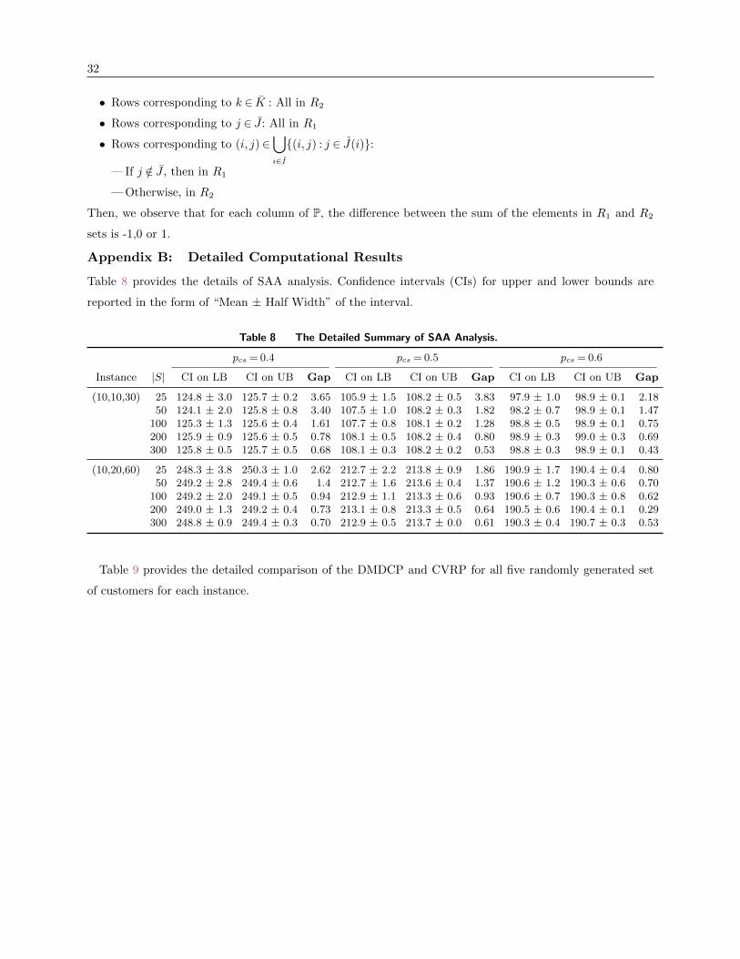
32

• Rows corresponding to k ∈ K : All in R2

• Rows corresponding to j ∈ J : All in R1

• Rows corresponding to (i, j)∈⋃i∈I

{(i, j) : j ∈ J(i)}:

— If j /∈ J , then in R1

— Otherwise, in R2

Then, we observe that for each column of P, the difference between the sum of the elements in R1 and R2

sets is -1,0 or 1.

Appendix B: Detailed Computational Results

Table 8 provides the details of SAA analysis. Confidence intervals (CIs) for upper and lower bounds are

reported in the form of “Mean ± Half Width” of the interval.

Table 8 The Detailed Summary of SAA Analysis.

pcs = 0.4 pcs = 0.5 pcs = 0.6

Instance |S| CI on LB CI on UB Gap CI on LB CI on UB Gap CI on LB CI on UB Gap

(10,10,30) 25 124.8 ± 3.0 125.7 ± 0.2 3.65 105.9 ± 1.5 108.2 ± 0.5 3.83 97.9 ± 1.0 98.9 ± 0.1 2.1850 124.1 ± 2.0 125.8 ± 0.8 3.40 107.5 ± 1.0 108.2 ± 0.3 1.82 98.2 ± 0.7 98.9 ± 0.1 1.47

100 125.3 ± 1.3 125.6 ± 0.4 1.61 107.7 ± 0.8 108.1 ± 0.2 1.28 98.8 ± 0.5 98.9 ± 0.1 0.75200 125.9 ± 0.9 125.6 ± 0.5 0.78 108.1 ± 0.5 108.2 ± 0.4 0.80 98.9 ± 0.3 99.0 ± 0.3 0.69300 125.8 ± 0.5 125.7 ± 0.5 0.68 108.1 ± 0.3 108.2 ± 0.2 0.53 98.8 ± 0.3 98.9 ± 0.1 0.43

(10,20,60) 25 248.3 ± 3.8 250.3 ± 1.0 2.62 212.7 ± 2.2 213.8 ± 0.9 1.86 190.9 ± 1.7 190.4 ± 0.4 0.8050 249.2 ± 2.8 249.4 ± 0.6 1.4 212.7 ± 1.6 213.6 ± 0.4 1.37 190.6 ± 1.2 190.3 ± 0.6 0.70

100 249.2 ± 2.0 249.1 ± 0.5 0.94 212.9 ± 1.1 213.3 ± 0.6 0.93 190.6 ± 0.7 190.3 ± 0.8 0.62200 249.0 ± 1.3 249.2 ± 0.4 0.73 213.1 ± 0.8 213.3 ± 0.5 0.64 190.5 ± 0.6 190.4 ± 0.1 0.29300 248.8 ± 0.9 249.4 ± 0.3 0.70 212.9 ± 0.5 213.7 ± 0.0 0.61 190.3 ± 0.4 190.7 ± 0.3 0.53

Table 9 provides the detailed comparison of the DMDCP and CVRP for all five randomly generated set

of customers for each instance.

33

Table 9 Detailed Sensitivity Analysis Results to Compare the DMDCP and CVRP.

CVRP costDMCDPcost saving

µ Instance DMCDP Q= 5 Q= 10 Q= 5 Q= 10

1.0 (10,10,30) 79.7 110.3 83.8 27.7 4.965.4 112.4 84.6 41.8 22.783.4 124.6 92.1 33.1 9.480.0 115.3 91.7 30.6 12.775.9 113.9 85.0 33.4 10.7

(20,20,60) 140.2 195.6 139.7 28.3 -0.4158.2 212.8 146.9 25.6 -7.7150.3 208.7 138.7 28.0 -8.3192.9 194.4 131.9 0.8 -46.2172.7 191.1 136.1 9.6 -26.9

(20,30,90) 207.6 303.3 191.6 31.6 -8.4217.2 302.0 191.5 28.1 -13.4262.2 276.2 175.9 5.1 -49.0224.2 288.6 189.0 22.3 -18.7228.6 282.2 187.7 19.0 -21.8

1.5 (10,10,30) 98.7 165.5 125.8 40.3 21.584.4 168.6 127.0 49.9 33.5

102.4 187.0 138.1 45.2 25.9100.5 172.9 137.5 41.9 26.996.4 170.8 127.5 43.6 24.4

(20,20,60) 175.2 293.4 209.6 40.3 16.4193.6 319.2 220.3 39.3 12.1187.8 313.1 208.1 40.0 9.8228.1 291.6 197.9 21.8 -15.3208.4 286.6 204.2 27.3 -2.0

(20,30,90) 262.6 454.9 287.3 42.3 8.6272.2 453.0 287.3 39.9 5.2314.8 414.3 263.9 24.0 -19.3279.3 432.9 283.5 35.5 1.5276.1 423.3 281.5 34.8 1.9

2.0 (10,10,30) 117.7 220.7 167.7 46.6 29.8103.4 224.8 169.3 54.0 38.9121.4 249.3 184.2 51.3 34.1120.6 230.6 183.3 47.7 34.2115.9 227.8 170.0 49.1 31.8

(20,20,60) 210.2 391.2 279.5 46.3 24.8228.6 425.5 293.8 46.3 22.2225.0 417.4 277.4 46.1 18.9261.8 388.9 263.8 32.7 0.8243.4 382.2 272.3 36.3 10.6

(20,30,90) 317.6 606.6 383.1 47.6 17.1327.2 604.1 383.0 45.8 14.6365.3 552.3 351.9 33.9 -3.8334.3 577.2 377.9 42.1 11.5321.1 564.4 375.3 43.1 14.5

stochastic last-mile delivery with crowd-shipping and ...about crowd-shippers and delivery tasks is...

Documents