Stochastic Gradient Descent Training for L1-regularizaed Log-linear Models with

Cumulative Penalty

Yoshimasa Tsuruoka, Jun’ichi Tsujii, and Sophia Ananiadou

University of Manchester

1

Log-linear models in NLP

• Maximum entropy models– Text classification (Nigam et al., 1999)– History-based approaches (Ratnaparkhi, 1998)

• Conditional random fields– Part-of-speech tagging (Lafferty et al., 2001),

chunking (Sha and Pereira, 2003), etc.• Structured prediction

– Parsing (Clark and Curan, 2004), Semantic Role Labeling (Toutanova et al, 2005), etc.

2

Log-linear models

Feature functionWeight

y

yxxi

ii fwZ ,exp

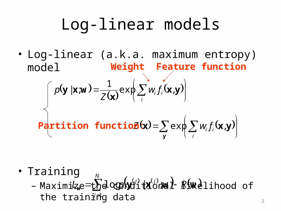
• Log-linear (a.k.a. maximum entropy) model

• Training– Maximize the conditional likelihood of the training data

Partition function:

iii fwZ

p yxx

wxy ,exp1

;|

wwxyw RpLN

j

jj 1

;|log

3

Regularization

• To avoid overfitting to the training data– Penalize the weights of the features

• L1 regularization

– Most of the weights become zero– Produces sparse (compact) models– Saves memory and storage

i

i

N

j

jj wCpL1

;|log wxyw

4

Training log-linear models

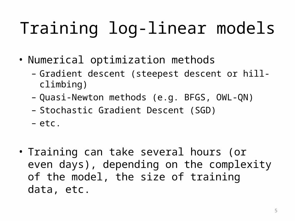
• Numerical optimization methods– Gradient descent (steepest descent or hill-climbing)– Quasi-Newton methods (e.g. BFGS, OWL-QN)– Stochastic Gradient Descent (SGD)– etc.

• Training can take several hours (or even days), depending on the complexity of the model, the size of training data, etc.

5

Gradient Descent (Hill Climbing)

1w

2w

objective

6

Stochastic Gradient Descent (SGD)

1w

2w

objective

Compute an approximate gradient using onetraining sample

7

Stochastic Gradient Descent (SGD)

• Weight update procedure– very simple (similar to the Perceptron algorithm)

Not differentiable

8

i

jj

i

ki

ki w

N

Cp

www wxy ;|log1

: learning rate

Using subgradients

• Weight update procedure

i

jj

i

ki

ki w

N

Cp

www wxy ;|log1

0if1

0if0

0if1

i

i

i

ii w

w

w

ww

9

Using subgradients

• Problems– L1 penalty needs to be applied to all features

(including the ones that are not used in the current sample).

– Few weights become zero as a result of training.

i

jj

i

ki

ki w

N

Cp

www wxy ;|log1

10

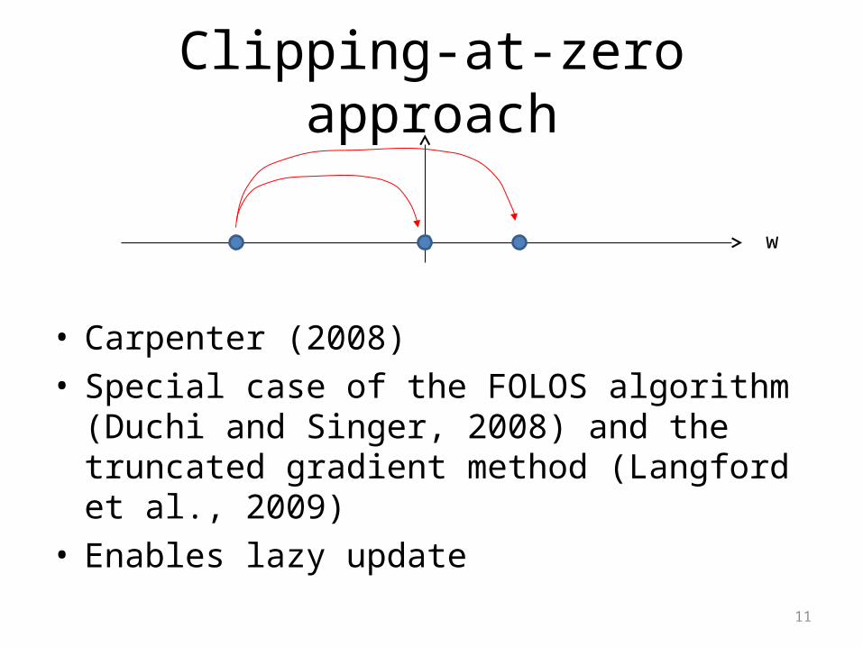
Clipping-at-zero approach

• Carpenter (2008)• Special case of the FOLOS algorithm (Duchi and

Singer, 2008) and the truncated gradient method (Langford et al., 2009)

• Enables lazy update

w

11

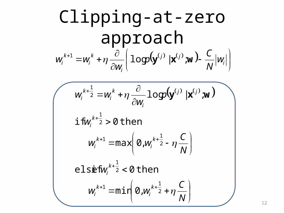
Clipping-at-zero approach

12

i

jj

i

ki

ki w

N

Cp

www wxy ;|log1

N

Cww

w

N

Cww

w

pw

ww

ki

ki

ki

ki

ki

ki

jj

i

ki

ki

2

11

2

1

2

11

2

1

2

1

,0min

then0ifelse

,0max

then0if

;|log wxy

• Text chunking

• Named entity recognition

• Part-of-speech tagging

13

Number of non-zero features

Quasi-Newton 18,109

SGD (Naive) 455,651

SGD (Clipping-at-zero) 87,792

Number of non-zero features

Quasi-Newton 30,710

SGD (Naive) 1,032,962

SGD (Clipping-at-zero) 279,886

Number of non-zero features

Quasi-Newton 50,870

SGD (Naive) 2,142,130

SGD (Clipping-at-zero) 323,199

Why it does not produce sparse models

• In SGD, weights are not updated smoothly

Fails to becomezero!

L1 penalty is wasted away

14

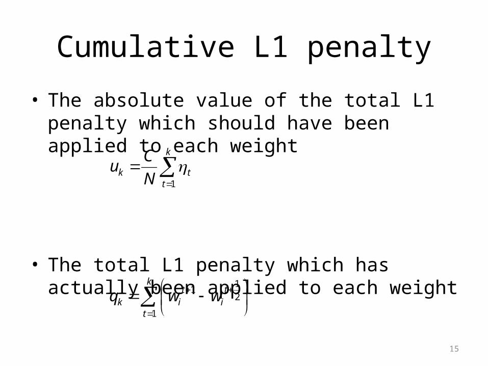
Cumulative L1 penalty

• The absolute value of the total L1 penalty which should have been applied to each weight

• The total L1 penalty which has actually been applied to each weight

15

k

ttk N

Cu

1

k

t

ti

tik wwq

1

2

11

Applying L1 with cumulative penalty

12

11

2

1

12

11

2

1

2

1

,0min

then0ifelse

,0max

then0if

;|log

kik

ki

ki

ki

kik

ki

ki

ki

jj

i

ki

ki

quww

w

quww

w

pw

ww wxy

• Penalize each weight according to the difference between and ku

1kiq

Implementation

10 lines of code!

17

Experiments

• Model: Conditional Random Fields (CRFs)• Baseline: OWL-QN (Andrew and Gao, 2007)• Tasks

– Text chunking (shallow parsing)• CoNLL 2000 shared task data• Recognize base syntactic phrases (e.g. NP, VP, PP)

– Named entity recognition• NLPBA 2004 shared task data• Recognize names of genes, proteins, etc.

– Part-of-speech (POS) tagging• WSJ corpus (sections 0-18 for training)

18

CoNLL 2000 chunking task: objective

19

CoNLL 2000 chunking: non-zero features

20

CoNLL 2000 chunking

Passes Obj. # Features Time (sec) F-score

OWL-QN 160 -1.583 18,109 598 93.62

SGD (Naive) 30 -1.671 455,651 1,117 93.64

SGD (Clipping + Lazy Update) 30 -1.671 87,792 144 93.65

SGD (Cumulative) 30 -1.653 28,189 149 93.68

SGD (Cumulative + ED) 30 -1.622 23,584 148 93.66

21

• Performance of the produced model

• Training is 4 times faster than OWL-QN• The model is 4 times smaller than the clipping-at-zero approach• The objective is also slightly better

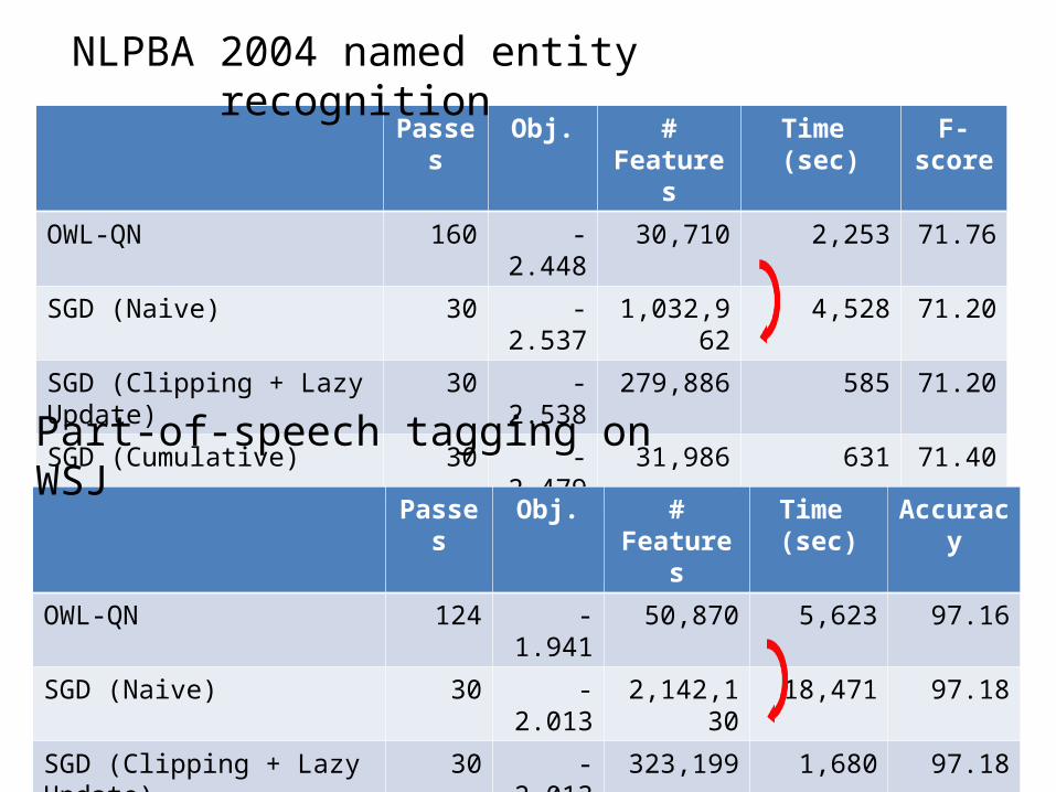
Passes Obj. # Features Time (sec) F-score

OWL-QN 160 -2.448 30,710 2,253 71.76

SGD (Naive) 30 -2.537 1,032,962 4,528 71.20

SGD (Clipping + Lazy Update) 30 -2.538 279,886 585 71.20

SGD (Cumulative) 30 -2.479 31,986 631 71.40

SGD (Cumulative + ED) 30 -2.443 25,965 631 71.63

NLPBA 2004 named entity recognition

22

Passes Obj. # Features Time (sec)

Accuracy

OWL-QN 124 -1.941 50,870 5,623 97.16

SGD (Naive) 30 -2.013 2,142,130 18,471 97.18

SGD (Clipping + Lazy Update) 30 -2.013 323,199 1,680 97.18

SGD (Cumulative) 30 -1.987 62,043 1,777 97.19

SGD (Cumulative + ED) 30 -1.954 51,857 1,774 97.17

Part-of-speech tagging on WSJ

Discussions

• Convergence– Demonstrated empirically– Penalties applied are not i.i.d.

• Learning rate– The need for tuning can be annoying– Rule of thumb:

• Exponential decay (passes = 30, alpha = 0.85)

23

Conclusions

• Stochastic gradient descent training for L1-regularized log-linear models– Force each weight to receive the total L1 penalty

that would have been applied if the true (noiseless) gradient were available

• 3 to 4 times faster than OWL-QN• Extremely easy to implement

24