stochastic financial analytics for cash-flow …
TRANSCRIPT

The Pennsylvania State University
The Graduate School
College of Engineering
STOCHASTIC FINANCIAL ANALYTICS FOR CASH-FLOW BULLWHIP,
CASH-FLOW FORECAST, AND WORKING CAPITAL OPTIMIZATION
A Dissertation in
Industrial and Manufacturing Engineering
by
Rattachut Tangsucheeva
2014 Rattachut Tangsucheeva
Submitted in Partial Fulfillment
of the Requirements
for the Degree of
Doctor of Philosophy
August 2014

The dissertation of Rattachut Tangsucheeva was reviewed and approved* by the following:
Vittaldas V. Prabhu
Professor of Industrial and Manufacturing Engineering
Dissertation Advisor
Chair of Committee
A. Ravi Ravindran
Professor of Industrial Engineering, Chair-Enterprise Integration Consortium
Tao Yao
Associate Professor of Industrial and Manufacturing Engineering
Douglas Thomas
Professor of Supply Chain and Information Systems, MBA Faulty Director
Paul Griffin
Peter and Angela Dal Pezzo Department Head Chair
Head of the Department of Industrial and Manufacturing Engineering
*Signatures are on file in the Graduate School

iii
ABSTRACT
Managing modern supply chains involves dealing with complex dynamics of materials,
information, and cash flows around the globe, and is a key determinant of business success today.
One of the well-recognized challenges in supply chain management is the inventory bullwhip
effect in which demand forecast errors are amplified as it propagates upstream from a retailer, in
part because of lags and errors in information flows. Adverse effects of such bullwhip
effect include excessive inventory, stock-outs, backorders, and wasteful swings in manufacturing
production. In this dissertation we theorize that inventory bullwhip also leads to cash-flow
bullwhip (CFB). Specifically, this research focuses on studying CFB by developing mathematical
and simulation models to analyze the relationship between inventory and cash-flow bullwhip by
using Cash Conversion Cycle (CCC) as a metric. CFB predicted by the proposed mathematical
models approximately differ 14% from detailed simulation models. We find that increasing
variability increases inventory and cash-flow bullwhip along with lead time, whereas increasing
the demand observation period has the opposite effect. The average marginal impact of the
bullwhip effect on the CFB is approximately 20%. Additionally, the CFB is also an increasing
function of an expected value of inventory and a decreasing function of an expected value of
demand.
Next, we develop stochastic financial analytics for cash flow forecasting for firms by
integrating two models: (1) Markov chain model of the aggregate payment behavior across all
customers of the firm using accounts receivable aging and; (2) Bayesian model of individual
customer payment behavior at the individual invoice level. As the stochastic dynamics of cash
flow evolves every day, the forecast can be updated every time an invoice is paid. The proposed
model is back-tested using empirical data from a small manufacturing firm and found to differ
3%-6% from actual monthly cash flow, and differs approximately 2%-4% compared to actual

iv
annual cash flow. The forecast accuracy of the proposed stochastic financial analytics model is
found to be considerably superior to other techniques commonly used. Furthermore, in computer
simulation experiments, the proposed model is found to be largely robust to supply chain
dynamics, including when subjected to severe bullwhip effect. The proposed model has been
implemented in Excel, which allows it to be easily integrated with the accounts receivable aging
data, making it practicable for small and large firms.
Lastly, we identify a potential strategy to engineer a solution for dynamic financial
decisions. This part focuses on maximizing profit of two types of manufacturing firms: firms with
non-recurring customers and firms with recurring customers. The proposed model determines the
optimal pricing of products sold to different customers using an integer programming model in
which Friedman’s model is used to estimate bid winning probability and the model is constrained
by several operational factors including working capital and customer credit risk. Customer credit
risk is modeled as the probability of payment delay or default, which is used to add a risk
premium into the bid price. The model can be used for decision-support in business development
to select an optimal portfolio of customer projects or bids to pursue. Detailed industrial case
studies used to test the efficacy of the proposed model show that the Price/Cost ratio has an
inversely proportional relationship to the winning probability, and the winning probability has the
inversely proportional relationship to the risk premium. However, at a high winning probability,
the firm may not be able to make a profit due to the unrealistically low bidding price. The results
also show the bidding price at which the firm is expected to maximize its profit.

v
TABLE OF CONTENTS
List of Figures .......................................................................................................................... vii
List of Tables ........................................................................................................................... ix
Acknowledgements .................................................................................................................. x
Chapter 1 INTRODUCTION ................................................................................................... 1
1.1 Background ................................................................................................................ 1 1.2 Motivation .................................................................................................................. 6 1.3 Research and objectives ............................................................................................. 7 1.4 Research Contributions .............................................................................................. 8 1.5 Outline of the Dissertation ......................................................................................... 9
Chapter 2 LITERATURE REVIEW ........................................................................................ 11
2.1 Cash Flow Management ............................................................................................. 11 2.2 Cash Flow Forecast .................................................................................................... 17 2.3 Cash Flow Risk .......................................................................................................... 19 2.4 Credit Risk ................................................................................................................. 20 2.5 Dynamic Financial Decisions .................................................................................... 22 2.6 Integration of Cash Flow and Supply Chain .............................................................. 24 2.7 Bullwhip Effect and Cash Flow ................................................................................. 28
Chapter 3 MODELING AND ANALYSIS OF CASH-FLOW BULLWHIP IN SUPPLY
CHAIN ............................................................................................................................. 30
3.1 Introduction ................................................................................................................ 30 3.2 Analytical Model for CFB ......................................................................................... 34
3.2.1 Impact on Inventory in Simple Supply Chain ................................................. 34 3.2.2 Impact on Inventory in Multi-Stages Supply Chain with Centralized
Demand Information ........................................................................................ 42 3.2.3 Impact on CCC in Simple Supply Chain ......................................................... 48
3.3 Simulation Model ....................................................................................................... 55 3.4. Results and Discussion .............................................................................................. 58
3.4.1 Impact on the Inventory Variance ................................................................... 58 3.4.2 Impact on the CFB .......................................................................................... 60
3.5 Conclusions ................................................................................................................ 68
Chapter 4 STOCHASTIC FINANCIAL ANALYTICS FOR CASH FLOW
FORECASTING .............................................................................................................. 70
4.1 Introduction ................................................................................................................ 70 4.2 Stochastic Financial Analytics Model ........................................................................ 74 4.3 Enterprise Level Application ..................................................................................... 85 4.4 Supply Chain Level Application ................................................................................ 99
4.4.1 Bullwhip Effect (BWE) ................................................................................... 99

vi
4.4.2 Inventory Bullwhip (IBW) .............................................................................. 100 4.4.3 Cash Flow Bullwhip (CFB) ............................................................................. 101 4.4.4 Simulation Model ............................................................................................ 102
4.5 Conclusions ................................................................................................................ 107
Chapter 5 OPTIMAL PRICING WITH CONSTRAINTS ON WORKING CAPITAL
AND PAYMENT DELAY RISK .................................................................................... 110
5.1 Introduction ................................................................................................................ 110 5.2 Pricing Model ............................................................................................................. 115
5.2.1 Objective Functions ......................................................................................... 115 5.2.2 Constraints ....................................................................................................... 117
5.3 Industrial Case Numerical Examples ......................................................................... 123 5.3.1 Industrial Case - Firm with Non Recurring Customers ................................... 124 5.3.2 Industrial Case - Firm with Recurring Customers ........................................... 128
5.4 Results and Discussion ............................................................................................... 131 5.5 Conclusions ................................................................................................................ 137
Chapter 6 CONCLUSIONS AND FUTURE DIRECTIONS .................................................. 139
6.1 Conclusions ................................................................................................................ 139 6.2 Future Directions ........................................................................................................ 142
References ................................................................................................................................ 144
Appendix A PROOF OF EQUATION (3.8) ........................................................................... 161
Appendix B PROOF OF EQUATION (3.10) ......................................................................... 168

vii
LIST OF FIGURES
Figure 1-1. Flows in supply chain. ......................................................................................... 2
Figure 2-1. Saw tooth cash balance (Miller and Orr, 1966). .................................................... 13
Figure 2-2. Real cash balance (Miller and Orr, 1966). ............................................................ 14
Figure 2-3. Supply network (Fayazbakhsh and Razzazi, 2008). .............................................. 28
Figure 3-1. Bullwhip effect of material flow in the supply chain. ........................................... 31
Figure 3-2. Effect of lead time L on inventory bullwhip. ........................................................ 40
Figure 3-3. Effect of demand observation period p on inventory bullwhip ............................. 41
Figure 3-4. Effect of lead time L on retailer CFB. ................................................................... 53
Figure 3-5. CFB corresponding to the bullwhip effect and p value. ........................................ 54
Figure 3-6. CFB corresponding to the bullwhip effect and value. ........................................ 54
Figure 3-7. CFB corresponding to the E(I) and E(D). ............................................................. 55
Figure 3-8. Model logic for each supply chain stage. .............................................................. 57
Figure 3-9. Variance of inventory versus bullwhip effect. ...................................................... 59
Figure 3-10. Inventory level over time. ................................................................................... 60
Figure 3-11. Cash Flow Bullwhip (Var (CCC)/Var(D)) vs Bullwhip Effect
(Var(q)/Var(D)). ............................................................................................................... 61
Figure 3-12. CFB over time, (a) Retailer, (b) Distributor, and (c) Manufacturer. ................... 63
Figure 3-13. Var(I)/Var(D) over time, (a) Retailer, (b) Distributor, and (c) Manufacturer. .... 64
Figure 3-14. CFB over lead time L, (a) Retailer, (b) Distributor, and (c) Manufacturer. ........ 66
Figure 3-15. Var(I)/Var(D) over lead time L, (a) Retailer, (b) Distributor, and (c)
Manufacturer. ................................................................................................................... 67
Figure 4-1. Bullwhip Effect and Cash Flow Bullwhip in the supply chain. ............................ 73
Figure 4-2. (a) Model concept and (b) process of the proposed cash flow forecast. ............... 76
Figure 4-3. Markov chain state diagram. ................................................................................. 79
Figure 4-4. Weibull distribution with the shape parameter k = 1, 2, and 5, respectively......... 81

viii
Figure 4-5. Transition Matrix T2. ............................................................................................. 88
Figure 4-6. Exponentially Smoothed Matrix and , and Forecasted vector F3. ............. 88
Figure 4-7. Forecasting accuracy and and value. ............................................................... 89
Figure 4-8. Sensitivity analysis of and for quarter 1, 2, 3, and 4. ..................................... 91
Figure 4-9. Cash flow from actual cash flow and various forecasting models. ....................... 93
Figure 4-10. Percent difference of forecasting models. ........................................................... 94
Figure 4-11. Average percent monthly difference. .................................................................. 94
Figure 4-12. Accumulated percent annually difference. .......................................................... 95
Figure 4-13. Forecasting differences (monthly). ..................................................................... 96
Figure 4-14. Average forecasting difference (monthly). ......................................................... 97
Figure 4-15. Forecasting difference (annually). ....................................................................... 98
Figure 4-16. Average forecasting difference (annually). ......................................................... 99
Figure 4-17. Structure of a supply chain in this simulation. .................................................... 103
Figure 4-18. Comparison among five techniques at a manufacturer stage. ............................. 105
Figure 4-19. Cash flow forecast difference at different stages of supply chain (Moving
average). ........................................................................................................................... 106
Figure 4-20. Cash flow forecast difference at different stages of supply chain (Proposed
model). ............................................................................................................................. 106
Figure 5-1. Phase classification of design project bidding decision (Wang et al., 2009). ....... 111
Figure 5-2. Scenario diagram of the MTO firm bidding. ......................................................... 113
Figure 5-3. Winning probability (a) and Bidding pattern of average bidder (b). ..................... 132
Figure 5-4. Expected profit over Price-Cost ratio (PC ratio). .................................................. 133
Figure 5-5. Expected profit vs Credit risk................................................................................ 134
Figure 5-6. Winning probability vs Credit risk. ....................................................................... 134
Figure 5-7. Expected profit vs Winning probability. ............................................................... 135
Figure 5-8. Expected profit vs Working capital. ...................................................................... 135

ix
LIST OF TABLES
Table 3-1. Comparison of average results of the analytical model with the simulation. ........ 62
Table 4-1. State definition. ...................................................................................................... 77
Table 4-2. Accounts Receivable Aging and Bad Debt. .......................................................... 78
Table 4-3. Cash Flow and Forecasting Difference of Customer #1. ....................................... 92
Table 5-1. Objective function parameters. .............................................................................. 126
Table 5-2. Various bidding price vs expected profit. .............................................................. 127
Table 5-3. Bidding prices and expected profits ...................................................................... 127
Table 5-4. Constraint parameters. ........................................................................................... 128
Table 5-5. Upper and Lower bound. ....................................................................................... 128
Table 5-6. Objective function parameters. .............................................................................. 129
Table 5-7. Bidding prices and expected profits ...................................................................... 130
Table 5-8. Constraint parameters. ........................................................................................... 130
Table 5-9. Upper and Lower bound. ....................................................................................... 130
Table 5-10. Results. ................................................................................................................ 131
Table 5-11. Results for 6 periods. ........................................................................................... 136

x
ACKNOWLEDGEMENTS
I would never have been able to finish my dissertation without the valuable guidance
from my committee members: Dr. Ravindran, Dr. Yao, and Dr. Thomas, help from friends and
support from my family.
I would like to express my deepest gratitude to my advisor, Dr. Vittaldas Prabhu, for his
excellent guidance, caring, patience, and providing me with an excellence atmosphere for doing
research.
I would like to thank Sriramprasad Sasisekaran, who was partially programmed the
simulation in Chapter 3. Many thanks to fellow students in the DISCRETE lab, friends, and Thai
friends for their friendship and support.
Finally, I thank my parents, and my wife Poravee for their love, support and always stand
by me for both good and bad times.

1
Chapter 1
INTRODUCTION
1.1 Background
Supply chain management is currently a fast growing area in most businesses and is
considered as key to the success of most leading companies. Supply chain is a dynamic system
involving coordination of three major flows, which are product flow, financial flow, and
information flow, between different supply chain stages such as supplier, manufacturer,
wholesaler, distributor, and retailer (Chopra and Meindl, 2007). Typically, a stage of a supply
chain can be one of these following processes: sourcing, manufacturing, distributing,
transporting, and retailing. However, it is not necessary for a supply chain to contain all the
processes above. For example, the manufacturer may produce and ship products directly to
retailers. Therefore, in this case, the supply chain does not contain a distributor.
Figure 1-1 shows product flow, financial flow, and information flow, between a supplier
and a manufacturer at one stage of a multi-stage supply chain. These flows continue in all stages
across the supply chain.
Product flow starts from a supplier providing raw materials or parts to a manufacturer.
Then a manufacturer begins manufacturing processes and then ships finished products to a
distributor who transfers the replenishment orders to retailers. Eventually, retailers fill orders to
its customers. Understanding these fundamental product flows provide us a big picture of how
products move from place to place and real understanding in order to improve the cash flow of a
supply chain. Financial flow usually transfers backward which is different from that of the
product flow.

2
Figure 1-1. Flows in supply chain.
Financial flow starts from customers making payments to retailers. Then, the retailers pay
the bills to their distributors and the distributors pay to their manufacturers, and manufacturers
pay to their suppliers.
Information flow plays an important role to a supply chain management because it
analogously functions as a bridge to link among other supply chain drivers which are facilities,
inventory, transportation, information, sourcing, and pricing. A goal of good information flow is
to integrate and coordinate factors in a supply chain for a decision maker to execute transactions.

3
Information makes a supply chain visibility. Without it, a manager is blind and unable to know
what the demand of products is, how much products left in stock, how much more to produce and
ship these products (Chopra and Meindl, 2007). A lack of supply chain coordination may cause
negative effects to the performance of the supply chain such as the Bullwhip effect. Therefore,
accurate information is crucial to the decision making and the performance of a supply chain.
In a real business world, a manufacturer may have several sources of raw material from
many suppliers from many locations shipped to assemble and then distribute the finished products
to many distributors and retailers. For a larger and more complex supply chain containing more
than one suppliers, manufacturers, distributors, and retailers, it is probably more accurate to call a
supply network rather than a supply chain (Chopra and Meindl, 2007). Moreover, in this
globalization era in which modern communications and transportation technologies have been
developed tremendously, a supply network may have suppliers and retailers located in different
continent where it can have competitive advantages. A supply network, which has sources of raw
material, manufactures products, and sells to its customers in more than one country is considered
be a global supply network. The growing internationalization of American business increased
sharply in year 1998 to 2000 and the cumulative foreign direct investment in the U.S. from 2008
to 2012 reached $2.65 trillion (Shapiro, 2006; investment, 2013). The internationalization of
commerce provides firms to seek for raw materials, markets, and cost minimization. For example,
an mp3 player from Apple Inc. called iPod, it was engineered in India, designed in America,
manufactured in China and sold around the world (Ravindran, 2008).
Even though the structure and size of a supply chain is varied, it focuses on the same
direction where its objective is the same as that of commercial firms, maximize overall profit.
The higher the profit, the more successful the supply chain is. The source of revenues comes from
customers who pay positive cash flow; whereas, other activities in product, information and
financial flows incur cost into the supply chain (Chopra and Meindl, 2007). Therefore, a good

4
supply chain management plays an important role to a successive firm in this competitive
business world.
Generally, financial management is categorized into two basic functions: (1) the
acquisition of funds and (2) the investment of those funds. The first function, also known as the
financing decision, involves the processes to acquire funds from both internal and external
sources to the firm at the lowest cost possible. This also includes how to transfer funds from place
to place when buying raw materials and selling products. The second function, the investment
decision, involves allocation of funds to earn maximum profit.
Other financial management, for example, internal financial flow of a corporate such as
loan repayments usually is achieved by accessing to sources of funds that are already exist. Other
financial flows, such as dividend payments, may be managed to provide to shareholders in order
to reduce tax burdens or currency risk. Capital structure and other financing decisions are usually
undertaken to reduce investment risks and financing costs. These actions frequently are motivated
by firm’s financial situation and world’s economic status at that time.
However, in the current economic downturn and credit squeeze, sales are dropping, cash
reserves are decreasing, and banks are very careful to lend money. Only a good supply chain
management may not adequate for a firm to survive in this critical situation. A firm has to pay
more attention to the importance of cash flow and working capital management. Particularly, a
multinational corporate should focus on real-time visibility of cash balance among corporations
worldwide. Cash flow is crucial of survivability of a firm. Without cash a firm fails to meet basic
financial obligations such as payroll, taxes, and payment to suppliers (Pate-Cornell et al., 1990).
All these factors eventually may risk a firm with a poor cash flow management bankruptcy.
Cash flow forecasting is one of the keys for efficient cash flow management and business
operation. Nonetheless, each company may have different purposes for its cash flow forecast. A
company, such as a start-up company, may just want to forecast its cash flow in order to know

5
how fast it uses up cash and whether it needs to prepare for additional funds whereas a big
company may want to perform the forecast to maximize its return on investment. More generally,
most companies may simply want to manage their obligations such as debt repayment, wages,
and so forth. Therefore, the use of the cash position forecast for treasury roles can be summarized
as follows (WWCP, 2012):
1. To meet external obligations
2. To minimize external borrowing costs
3. To maximize investment outcomes
4. To manage currency exposure
In addition to the usage of the core treasury roles, the company may also use the cash
position forecast in order to exercise control over group companies, to perform a general
management role, and to perform a strategic role. Despite great benefits of the forecast, most
SMEs fail to do it because they may not have sufficient and effective resources to do so. Some of
the difficulties in cash position forecasting are as follows (WWCP, 2012).
1. Different countries and time zones
2. Complexity of data integration from other external sources
3. Multicurrency forecasts
4. Status and quality of underlying data
Therefore, effective cash and liquidity management are ultimately important at all times,
especially during this economic downturn time. A firm must enhance its treasury functions
throughout its branches and subsidiaries to achieve accurate and real-time visibility of its cash
balances. Effective financial manager should be able to acquire cash whenever it is required and
minimize the need for unnecessary borrowing. The challenging problem is to formulate

6
relationships between supply chain management and cash flow management to improve cash flow
in a supply chain by integrating these two concepts together.
1.2 Motivation
Among the product flow, information flow, and financial flow of a supply chain, previous
supply chain studies focused more on the first two flows. However, the relationship between the
product flow and financial flow, in particular, cash flow, is less explored (Comelli et al., 2008;
Tsai, 2008). Cash is not only an essential resource needed to support almost all activities in a
firm; it also provides liquidity for companies during financial difficult time and allows them to
take advantage of expansion during the good time. Particularly, in a growth firm with few
customers or a firm paying high interest rate, good cash flow management is very essential
(Milling, 1983). A firm with high growth rate requires a large amount of capital to expand its
factory, hire more personnel, and increase inventory level in anticipation of high demand. Thus, a
high growth firm generally has large financial burden to pay in a near term whereas the source of
revenue comes from a small group of customers, which leads to increasing in uncertainty of
revenue. Finally, a high interest rate can incur a high cost of borrowing and a high opportunity
cost to maintain high cash balances.
For any supply chain, since revenues only come from customers who pay for products or
services, other activities in supply chain flows (product, information, and financial flows)
generate cost to the supply chain (Chopra and Meindl, 2007). Thus, most previous researches
focused on improving product flow, which is one way to reduce the cost of supply chain flows.
Many existing studies have done reducing the cost of product flow such as the just-in-time system
(JIT) and economic order quantity (EOQ) model. The goal of JIT is simply that the required parts
from upstream workstations are received precisely as needed (just in time) which could be done

7
by eliminating waste or having zero inventories in order to reduce cost (Hopp and Spearman,
2001). The EOQ model aims to optimize the order quantity to minimize the total cost, which
contains fixed ordering cost, holding cost, and unit cost.
The problem of cash flow management, especially during the economic downturn, and
the lack of researches that integrate between product flow and financial flow of a supply chain,
therefore, inspires this research to focus on the relationship between these two flows of a firm in
supply chain in order to optimize the maximize profit of a firm within a limited cash flow. So, a
financial manager can maintain minimum cash balance to sufficiently run a business (because
cash sitting in the account does not generate income) and prepare extra cash when it is needed to
prevent from cash shortage.
1.3 Research and objectives
Managing modern supply chains involves dealing with complex dynamics of materials,
information, and cash flows around the globe, and is a key determinant of business success today.
One of the well-recognized challenges in supply chain management is the inventory bullwhip
effect in which demand forecast errors are amplified as it propagates upstream from a retailer, in
part because of lags and errors in information flows. Adverse effects of such bullwhip
effect include excessive inventory and wasteful swings in manufacturing production. In this
dissertation we postulate that there can be a corresponding bullwhip in the cash flow across the
supply chain and it can be one of many reasons why firms run out of cash. Furthermore, we
explore ways to predict cash flow using stochastic financial analytics model to develop the
forecast model and finally identify a potential strategy to engineer a solution for maximizing
profit within a limited working capital by using mixed integer linear programming.

8
The ultimate goal of this research is to develop an integrated model that combines the
supply chain management concept and financial management concept together to maximize profit
of a firm. The integrated model is the dynamic financial decision model in order to assist a
manager to optimize the decision on cash flow in supply chain. The cost of shortage of cash flow
and the cost of credit risk are involved while maintaining adequate cash balance to run a business.
In developing an analytical model to express relationships between the product flow and cash
flow, there are some involvements of uncertainties from demand forecast and payment delay,
which need stochastic process to assist in formulating this model. While a rich historical research
and body of literature on supply chain and cash management exists separately, there is a gap
between the literature and this research to combine the concept of supply chain management and
cash flow management together.
1.4 Research Contributions
Some of the key concepts and the potential research contributions of this research are
summarized below:
1. The analytical models of the inventory bullwhip and the cash flow bullwhip in a supply
chain enable firms to better understand the phenomenon and the relationship among
inventory, bullwhip effect, and the cash flow bullwhip. These models lead to the
estimation of the cash flow bullwhip in a supply chain and how to reduce its adverse
impacts. The cash flow bullwhip can also be potentially set as a benchmark to measure
performance among supply chains.
2. The stochastic financial analytics model for cash flow forecasting is back-tested using
empirical data from a small manufacturing firm and found to be considerably superior to
other techniques commonly used. Furthermore, in computer simulation experiments, the

9
proposed model is found to be largely robust to supply chain dynamics, including when
subjected to severe bullwhip effect. The proposed model has been implemented in Excel,
which allows it to be easily integrated with the accounts receivable aging data, making it
practicable for small and large firms.
3. The optimal pricing model is able to provide a decision support to allocate proper amount
of investment in projects within limited working capital and selecting the projects that
maximize profit and minimize credit risk of a firm. The analysis also provides a better
understanding among price, cost, winning probability, profit, and credit risk. This leads to
some managerial insights and strategic planning to maximize profit.
1.5 Outline of the Dissertation
The remainder of this dissertation is organized into five chapters. First, Chapter 2
provides the comprehensive literature review related to cash flow. The review also includes cash
flow management in various situations and different objectives, cash flow forecast, cash flow
risk, credit risk, and cash flow decision. Lastly, this chapter provides the review of the
applications and integrations of cash flow management concept and supply chain management
concept that improve supply chain. Chapter 3 presents how to develop the analytical model of the
inventory bullwhip and the cash flow bullwhip. This model is extended from the quantitative
model of the bullwhip effect. Then the models are compared with the simulation model. In
Chapter 4, the stochastic financial analytics model for cash flow forecast is developed. The model
integrates the aggregate payment behavior across all customers of the firm using accounts
receivable aging and individual customer payment behavior at the individual invoice level to
perform the cash flow forecast. The proposed model is back-tested using empirical data from a
small manufacturing firm and found to be significantly improved. Chapter 5 presents the optimal

10
pricing with constraints on working capital and payment delay risk. The model is developed to
assist management to allocate capital investment in projects within limited working capital and
selecting the projects that maximize profit and minimize credit risk of a firm. Finally, conclusions
of this dissertation and the direction for the future research are addressed in Chapter 6.

11
Chapter 2
LITERATURE REVIEW
This chapter provides a review of existing literature related to cash flow management in
general and cash flow in supply chain. The review also discusses several techniques to manage
cash flow in various dimensions such as cash balance optimization and financial planning. Then,
the importance of cash flow forecast and several approaches to predict the cash flow are
addressed. Next we review how the cash flow risk and credit risk are measured, how cash flow is
impacted by these risks, and how these risks are mitigated. Then, the dynamic financial decisions
and project selection are reviewed. This review includes allocate funds to projects and how to
select projects to achieve firm’s objective such as maximizing profit or minimizing risk. Finally,
previous works relating to an integration of cash flow and supply chain are summarized.
2.1 Cash Flow Management
Cash flow management is one of the top concerns of many small and medium enterprises
(SMEs). Especially, when the enterprise progresses through various life-cycle stages, they face
more problematic situations in managing their financial assets (Mcmahon, 2001). Furthermore,
SMEs usually incur high interest rate for any types of financial services due to their higher credit
risk, and resource constraints they face when they use financial services (Baas and Schrooten,
2006). The need for more careful and effective cash flow management is of critical importance to
researchers and managers of SME’s.
Cash flow of a supply chain refers to the movement of revenue (cash inflows) or expense
(cash outflows) stream through its business during a specific period. Financial flow can be

12
assessed from the financial statements, which are balance sheet, income statement, and cash flow
statement. In this research, we focus on the relationship between product flow and financial flow,
especially cash flow.
A substantial body of research has focused on improving supply chain product flows such
as work in process and inventory. For example, the work of Hopp and Spearman, 2001 focuses on
determining the relationship among work in process, cycle time, and throughput and Chauhan et
al., 2007proposed the scheduling technique to minimize work in process. Other works are focused
on optimizing inventory level (Tempelmeier, 2006; Wu and Hwang, 2011) while only limited
research focuses on improving cash flow.
Cash flow is one of the most important financial statistics. It can be used to measure rate
of return and liquidity of a firm. Cash flow determines business’s solvency. It is crucial for
business to survive. Without cash, a firm fails to meet basic financial obligation to its creditors,
employees, and the others. A firm with insufficient cash is likely to bankrupt if the insolvency
continue. Therefore, economists try to forecast and improve cash flow. In this literature reviews
show many researches attempted to forecast and improve cash flow.
The literature on cash flow management applying the inventory management concept has
developed more than a century. An early attempt of some economists and mathematicians to
manage a cash balance using the techniques in inventory management was provided by Baumol,
1952. Some similarities between managing cash balance and inventory balance was recognized.
Baumol, 1952 proposed a deterministic model where parameters such as cash outflow was
predetermined; interest rate and transfer fee were constant. This work implemented the classical
“lot size” model of the inventory management and aimed to optimize the amount of transferred
cash in order to minimize transfer cost and holding cost while maintaining sufficient cash balance
to pay the bills. In Baumol’s model, the cash inflows and cash outflows were assumed to be
predetermined. The cash inflows periodically flow into the noninterest cash account for operating

13
the firm while the cash outflows are constant rate expenditures. The cash balance corresponding
to this model is in the simple saw tooth pattern, which is shown in Figure 2-1.
Figure 2-1. Saw tooth cash balance (Miller and Orr, 1966).
However, in reality, the cash balance of the firm is not as simple as shown in Figure 2-1.
On the contrary, the cash balance normally fluctuates depending on the amount and timing of
cash inflows and cash outflows. It is more complex and fluctuates over time in both positive and
negative directions (Miller and Orr, 1966) as shown in Figure 2-2. The cash balance becomes
more complex for multinational corporations and global supply networks which internal and
external economical aspects such as exchange rates are involved. Miller and Orr (1966) assumed
cash balance to be a stochastic model rather than assuming that cash flow occurs constantly. The
net cash flows fluctuate over time. There were probabilities of cash balance to increase and
decrease. The objective function was to obtain the optimal level of cash balance while
minimizing the long-run average cost (Miller and Orr, 1966).
Cash ($)
Time

14
Figure 2-2. Real cash balance (Miller and Orr, 1966).
From Figure 2-2 we can see that in some point in time the firm may have very low cash
balance or even negative cash balance may be possible. This situation can damage the firm in
many ways such as reduce credibility and reliability to its suppliers and customers. Both studies
by Baumol, 1952 and Miller and Orr, 1966 focus on minimizing transfer cost between two
financial accounts to maintain cash balance to an adequate working level. These two models
introduce ideas and provide good foundation of how to manage cash balance by applying supply
chain concept. Meanwhile, these two models leave some opportunity for further improvement in
this area to be more practical in the real business world. Some assumptions can be relaxed. For
example, transfer cost is assumed to be a constant independent of the amount transferred which is
not practical. Clearly, there is an opportunity to further study in this area. There are many
dimensions that need to be addressed. By understanding the fundamental behavior of the supply
chain, the manufacturing system, and the cash flow forms the basis of this research.
Charnes et al., 1963 suggested that the financial planning and operation planning should
be considered together to improve the revenues of a firm. Robichek et al., 1965 recognized the
simultaneous approach of the short term and long term capital budget instead of compute it
sequentially. However, the linear programming and financial management were not able to
Cash ($)
Time
$
0

15
simply capture the overall financial solution because the whole financial problem was too
complex to be analyzed. Therefore, this work isolates the problem into sub-problems and then
determines the solutions (Robichek et al., 1965). Girgis, 1968 applied the inventory management
concept to the cash management by developing optimal policies for maintaining cash balance in
anticipation of future net expenses. The cash flow was assumed to be independent and identically
distributed as well as the holding cost and the shortage cost were assumed to be convex (Girgis,
1968). Gormley and Meade, 2007 proposed a dynamic simple policy (DSP) to minimize
transaction cost considering the cash balance as a stochastic problem and the cash flow were not
independent or identically distributed.
Some financial techniques have been developed to mitigate the currency exchange risk
such as options, forwards, and swaps. Kazaz et al., 2005 formulated the optimal policy, which
involves the impact of currency exchange rate uncertainty, for the production planning of a
multinational corporation. The two-stage recourse program, production hedging and allocation
hedging, was formulated to maximize expected profit. This two-stage stochastic program was
incorporated with exchange rate realizations. The first stage determines the production planning
of how much to produce and then the second stage allocates the production to markets (Kazaz et
al., 2005).
Managing a firm’s working capital is very important for its operational and financial
success. The objective is to maintain cash flow to sufficiently cover its short-term debt
obligations and day-to-day operating expenses meanwhile keeping excess cash as low as possible
since the firm does not earn profit from cash sitting in the account. In other words, the firm loses
the opportunity to make a profit from investing this excess cash in other assets such as security
assets. Sustainable working capital allows a firm to be more flexible to expand business, improve
liquidity, and enhance responsiveness to economic situation.

16
Improving working capital has become crucial to the growth and profitability of most
firms since working capital is very sensitive to cash flow fluctuations (Fazzari and Peterson,
1993). Most of the previous works relating to working capital focus on application of
procurement policy, production capacity, production planning, and scheduling problem under
working capital constraints (Chung and Lin, 1998; Guillen et al., 2006; Guillen et al., 2007;
Comelli et al., 2008; Zeballos and Seifert, 2013). Ke and Ai, 2008 determined superior ordering
point while achieving working capital target. Protopappa-Sieke and Seifert, 2010 proposed a
model to determine optimal purchasing order quantity under working capital restrictions and
payment delays.
A firm hold a large amount of cash in order to operate its daily activities smoothly.
Hence, efficient cash flow management and working capital management are highly beneficial to
firm’s financial status. Orgler (1970) documented that a firm should have sufficient amount of
cash to operate its normal business and also to prepare for unexpected situations since it is very
difficult to forecast the cash flow accurately and to have cash inflows and outflows synchronize
perfectly.
A perfect cash flow forecast is impossible because of the uncertainty of cash inflows.
Uncertainty may come from customer payment behavior, liquidity problems of customers, and
economic situation. Therefore, a firm creates a cash buffer by determining a lower and upper
bound of cash flow. There are two types of metrics that are widely used to optimize cash flow,
cash position and cash flow. Cash position tells the level of cash available at the end of the period
while cash flow tells the amount of cash generated during the period. Several techniques to
compute the optimal cash level were developed (Orgler, 1969; Miller and Orr, 1966). However,
Orgler (1969) assumed that the cash outflows are controllable and not stochastic; therefore, the
forecast of the cash outflows was developed by a deterministic model. On the other hand, the cash
inflows contain uncertainty, but they are predictable. In this case, a linear programming model

17
can be applied to optimize the cash flow level. These mathematical programming techniques are
very useful and practically efficient in a real world (Graham and Harvey, 2001).
Yet cash flow is usually restrained in the form of accounts receivable and is over looked
when a firm tries to optimize its working capital. A number of literatures in finance reveals
information about the fact of how much cash is locked up in the accounts receivable, inventories,
accounts payable, and working capital. Classic financial models, which relate to optimization of
current assets such as accounts receivable, show that the extension of the payment terms on the
accounts receivable is a tradeoff between controlling the risks of payment delay from customers
and gaining new customers (Michalski, 2007).
2.2 Cash Flow Forecast
Accurate cash flow forecasting models that are easy to use are becoming important for
businesses to manage their finances efficiently. Such models will be especially critical for SMEs
when liquidity and credit decrease in the economy. Cash flow forecast can be performed in
several ways depending on the nature of businesses and the purpose of the forecast. Basically, it
can be categorized into two core techniques: the receipts and disbursements forecast, and
statistical modeling such as moving average, exponential smoothing, regression analysis, and
distribution model (WWCP, 2012). There is no perfect technique for forecasting because each
company has its own unique financial activity and characteristics.
Groeye and Mellyn, 2000 showed that for the past 20 years, days of inventory reduced by
35% (to 48 days) whereas days of receivables reduced by only 16% (to 57 days). A significant
portion of a firm’s asset can be tied up in the accounts receivable rather than in the inventory
(Cyert et al., 1962). One of the reasons why a large number of assets are tied up in the accounts
receivable is that the focus of efforts for past years was on reducing the inventory in a system

18
while little effort was put on reducing days of outstanding accounts receivable. As a result,
payment delay and bad debt can lead to major problems that can jeopardize a company, especially
in the case of an SME. Therefore, an accurate cash flow forecast is essential for a company to be
able to prepare itself for an unexpected and undesirable financial situation.
Pate-Cornell et al., 1990 formulated a stochastic model for monitoring cash flow and
making a short term decision using a signal-response model (Pate-Cornell, 1986; Pate-Cornell et
al., 1990). Elton and Gruber, 1974 generally formulated dynamic programming models for the
cash management policies under different assumptions of transaction costs and demand for cash
Elton and Gruber, 1974.
Kaka, 1996 proposed a computer-based cash flow forecasting model applying cumulative
curves of corresponding parameters such as cash in and cash out. In addition, this model included
some of the risk associated with a firm since construction projects were known to encounter high
level of risk (Kaka, 1996). Navon, 1996 developed a cash flow management model for a
company-level by gathering as much as from the model’s database (Navon, 1996; Kaka and
Lewis, 2003) developed a computer-based model to forecast a company-level cash flow. The
model basically involved with many uncertainties and it was needed to update new data
frequently; hence, a fully stochastic simulation model and dynamic data updating were applied
(Kaka and Lewis, 2003).
While cash is very essential for running a business as a current asset, accounts receivable,
another current asset which can be converted into cash very quickly become more imperative in
business transactions because most of them are credit transactions where sellers offer their
customers payment terms rather than cash on delivery. However, if the receivables cannot be
collected on the due dates, sooner or later the company will be insolvent. In order to avoid this
crisis, a company must have good cash flow management, especially during the economic
recession where cash is the main bloodline for surviving in a business.

19
Accounts receivable aging is a technique to evaluate the financial health of a company by
identifying whether irregularities exist. It shows a company’s accounts receivable according to
the length of time the amounts have been outstanding. The typical aging time period is 30 days,
60 days, 90 days, and over 120 days. In 1962, Cyert, Davidson, and Thompson successfully
developed a model to estimate the allowance for doubtful accounts using a Markov chain
approach. This CDT model was made more practicable by Corcoran, 1978 by using exponential
smoothing to the transition matrix and changed the method of accounts receivable aging from the
oldest balance method to the partial balance method, which is more commonly the standard
practice in most businesses. In addition, this study focuses more on the transient state rather than
the steady state as in the CDT model (Corcoran, 1978). Kuelen et al., 1981 reexamined the CDT
model and found that the use of the total balance aging method in the model did not reflect the
real age of the dollars in the accounts. The model was modified in order to perform more
accurately (Kuelen et al., 1981).
2.3 Cash Flow Risk
Tsai, 2008 proposed a model to forecast a cash flow risk measured by its standard
deviation. The main purpose was to gain insight cash information in order to practically improve
the cash conversion cycle (CCC). CCC, known as cash-to-cash cycle or cash cycle, is one of the
widely used performance measures on cash flow (Tsai, 2008). Since cash itself is a non-
productive asset, excess cash apart from covering day-to-day operating expenses is maintained as
little as possible (Bertel et al., 2008). A firm has to utilize cash efficiently.
In order to reduce CCC, a firm can reduce days-in-inventory, shorten days-in-receivables,
and prolong days-in-payables. However, the study found that an early payment discount to reduce
days-in-receivables, which reduced CCC, increased cash inflow risks. The additional risk in the

20
cash inflow came from uncertain early collection pattern. This risk could be reduced in case that
early collection ratio was a constant. In other words, the more the early collection pattern was
known, the lower the risk. Since the cash inflow risks dominated the net cash flow risks,
therefore, reducing the cash inflow risks could reduce the overall cash flow risks (Tsai, 2008).
The firm with flexible credit lines from its lender could take advantage to tolerate more
risks such as shortening the credit period and offering early payment discount; whereas, the firm
with tight credit could also tolerate the cash inflow risks by having longer credit terms for better
future cash flow prediction. However, the latter case led to worse CCC. The author also showed
that the Asset Based Securities (ABS) was the best policy to finance account receivables in order
to reduce CCC and cash inflow risk (Tsai, 2008).
2.4 Credit Risk
The concept of credit risk assessment becomes more intriguing to many financial analysts
and practitioners in financial area. Over the last three decades, a considerable number of efforts
have focused on developing credit risk assessment in both theoretical and practical models.
Financial characteristics of a firm such as financial ratios and financial performance measures are
studied to determine their relationships with the credit risk. As a result, these relationships are
identified and included in the decision support models for a firm to improve accuracy of the credit
risk and creditworthiness assessment as much as possible. A comprehensive review of credit risk
assessment over the last two decades is presented by Altman and Saunders (1998).
To determine the optimal credit-granting decision which a firm has to tradeoff between
the risk of payment loss and the chance of earning more profit from granting credit, the credit risk
assessment must take both financial and non-financial aspects into consideration (Srinivasan and

21
Kim, 1987; Srinivasan and Ruparel, 1990). The information of creditworthy and insolvent firms
can be obtained when a firm seeks for line of credit from banks or financial institutions.
A large number of factors usually required to evaluate the credit risk is considered as one
of major obstacles for the credit risk assessment process. These factors include financial
characteristics of firms, qualitative and quantitative performance measures of firms,
macroeconomic factors such as inflation and interest rate. To evaluate the credit risk, credit
analysts have to look into all these factors, screen out the least relevant factors, and then focus
their analysis on the rest of the relevant factors. The other major obstacle is the aggregation of
these factors from the previous phase. The complexity of these factors and analysis make it more
difficult and time consuming to make a final credit risk assessment. This obstacle can lead to
conflicting results and decisions. During the final process of credit risk assessment, the credit and
financial analysts try to balance these conflicting criteria corresponding to their preference
system. Consequently, the optimal outcome can be concluded from an appropriate aggregation of
evaluation criteria [Bergeron et al., 1996].
Due to a large number of relevant factors and the complexity of the process to evaluate
the credit risk, the systematic credit risk assessment models are developed based on the sorting
approach. These models facilitate credit and financial analysts as evaluation systems to evaluate
credit risk of new firms which seek for financing and as screening tools for bank and financial
institution to evaluate existing borrowers (Lane, 1972; Grablowsky and Talley, 1981; Altman et
al., 1983; Srinivasan and Kim, 1987; Srinivasan and Ruparel, 1990).
Many articles and academic articles studied how optimal working capital can improve
financial status of companies, but these studies do not usually include credit risk into the project
selection problem with a working capital constraint. The question discussed in this dissertation
concerns the possibility of using integer programming in making decisions about selecting which
projects or customers should be invested in. This is certainly one of the most common objectives.

22
Therefore, this dissertation addresses the implementation of bidding strategies with the project
selection. The target is to obtain trade-off solutions during the routine practice preserving at most
the profit and liquidity while compensating risk. The main purpose of this dissertation is to
determine the optimal project selection that maximize profit and minimize credit risk. The
proposed formulation combines a project selection problem and a credit risk problem with a
working capital constraint using an integer programming approach.
2.5 Dynamic Financial Decisions
Dynamic financial decisions are decisions that involve: (1) determining the proper
amount of funds to employ in a firm; (2) selecting projects and capital expenditure analysis; (3)
raising funds on the most favorable terms possible; and (4) managing working capital such as
inventory and accounts receivable, while an environment changes over time leading to the change
in financial decision-making. This dissertation focuses on a combination of allocating proper
amount of investment in projects within limited working capital and selecting projects that
maximize profit and minimize credit risk of a firm.
The art and science of project selection plays a critical role in many firms. Firms in each
industry develop their own highly sophisticated methods to screen and select projects based on
their specific industrial characteristics. These methods are created to ensure that the selected
projects provide the highest benefits and a promising success. MTO firms take it very seriously to
select projects they want to bid since selection of the right projects for future investment is crucial
for the firms meanwhile selection of the wrong projects may risk the firms to loss. Generally,
firms have numerous opportunities to invest in several projects. However, with limited working
capital and other resources, the firms cannot pursue all opportunities that present themselves. The
best choice must be made to secure the most viable projects. Several priority systems and project

23
selection guidelines are developed in order to utilize firms’ resources effectively and balance
between opportunities and costs entailed by each alternative.
Project selection methods vary depending on the firms, the customers, the criteria, and
the characteristics of the projects. Some projects should be evaluated by qualitative approaches
such as SWOT analysis while the others should be evaluated by quantitative approaches such as
scoring models, economic model, cost-benefit analysis, etc. A number of decision support models
to assist firms to screen and select potential project candidates are developed in many areas.
Followings are examples of project selecting decision support models: dynamic selection of risky
capital investments (Cord, 1964; Magee, 1964; Hespos and Strassman, 1965; Prastacos, 1983),
allocation of strategic resources such as production capacities (Naylor, 1984), and dynamic
selection and trimming of R&D investments (Hess, 1962; Rosen and Souder, 1965; Atkinson and
Bobis, 1969; Flinn and Turban, 1970; Bobis et al., 1971; Aldrich and Morton, 1975; Hopp, 1987;
Popp, 1987; Gupta and Mandakovic, 1992) (Heidenberger, 1996).
Most project selection methods take profit and loss, cost and benefit, and working capital
into account. Therefore, asset management techniques are also applied in many project selections
with regard to financial aspects. Several business decisions such as manufacturing redesign and
capital budgeting are examples of where asset management can be applied. The former example
deals with managing locations, scheduling, and capacity changes in physical assets such as
production facility, warehouse, and distribution facility. The latter example involves the
allocation of financial assets such as allocating of capital to procure materials, produce products,
and invest in new facilities (Naraharisetti et al., 2008).
Financial aspects are seemed to be the most common basis for project appraisal, however,
there are other considerations that can be taken into account. Meredith and S.J., 1995 reported
other areas of considerations that affect the project selection. Such considerations are production
considerations, marketing considerations, personnel considerations, and administrative

24
considerations in addition to financial considerations. In addition to these considerations, risk of a
project uncertainty and risk of incomplete project information are factors that make the project
evaluation more complex and difficult. In most cases, decisions are efficiently successful when
they are made with accurate information and in a timely manner. Pascale et al. (1997) researched
ways to balance competing demands of time and benefits (Pascale et al., 1997).
2.6 Integration of Cash Flow and Supply Chain
Some previous works study on integration between supply chain concept and cash flow
concept together in order to improve the cash flow of a firm. A supply chain typically contains
many physical facilities such as manufacturing factories, distribution centers, and warehouses.
The supply chain usually involves three types of flows, which are forward physical flow,
backward financial flow, and backward information flow (Comelli et al., 2008). Many areas
indicate that supply chain can combine with cash flow management to improve cash flow of a
supply chain.
The following papers studied on the product flow and the financial flow of supply chain
in order to improve supply chain’s efficiency. Traditionally, these two flows are considered
separately; however, these two papers integrated product flow and financial flow together. The
information flow was out of their scopes. These two papers focused on supply chain planning;
however, one focused on the tactical planning, and the other one focused on operational planning.
Comelli et al., 2008 proposed an approach to evaluate a tactical production planning in
supply chains by integrating budget constraints into account. This paper aimed to maximize
supply chain evaluation function to achieve job schedules. The evaluation of supply chain
performance was usually based on quantitative parameters such as stock level and demand
satisfaction. The Activity Based Costing (ABC), cost drivers, and payment terms were

25
implemented to evaluate financial flow which was generated from the tactical production
planning; however, due to the difficulty in implementing ABC directly to supply chain activities,
many activities in supply chain such as sourcing and manufacturing were required to model with
the Supply-Chain Operations Reference (SCOR) process before implementing ABC model.
A computer model called PRocess EVAluation or PREVA to evaluate the planning was
proposed. The PREVA contained two main steps; (1) physical process evaluation and (2)
financial flow evaluation. The physical process evaluation created a physical flow planning. Then
this planning became an input data for the second step, the financial flow evaluation. This latter
evaluation contained mathematical model to compute cost of each process and integrate cash flow
into the physical flow. During the financial evaluation, it determined differences between
activity-based cost and transferred price (profit) of each process. These differences provided a
value creation assessment in every business unit. The evaluation function selected the planning
with the highest value (Comelli et al., 2008).
Rather than integrate financial aspects to the tactical planning like Comelli et al., 2008,
Bertel et al., 2008 proposed a method to integrate financial aspects into operational production
planning in order to obtain optimal solutions, particularly the stock level, for a supply chain
manager. This supply chain was modeled as a flowshop. In addition, since this supply chain was a
complex manufacturing system, the hybrid flowshop was implemented to this problem. The
hybrid flowshop or multiprocessor flowshop was a generalization of flowshop problems, which at
least one stage had several resources. Performance measures for this type of problems were
demand satisfaction, payback time, stocking cost, cash position, production cost and cash flow
(Bertel et al., 2008).
The method, which the authors proposed contained two steps: (1) multiprocessor
flowshop or hybrid flowshop generation and (2) cash management. The hybrid flowshop
generated sequences of jobs for the tactical planning. Next, the cash management adjusted the

26
balance between non-invested cash and security-invested cash in order to have sufficient cash to
cover the day-to-day operating expenses with minimum excess cash. In the cash management,
there was a mathematical model applying mixed integer linear programming (MILP) to determine
an optimal average cash position. The mathematical model was run by a mathematical
programming language (AMPL), and tested by CPLEX solver. Another method to schedule job
process was a heuristic model, which contained two algorithms. An algorithm1 applied greedy
search algorithm to schedule plant while an algorithm2 applied the BFRT algorithm to provide a
list of jobs to be processed.
Another study which integrated financial cross functions into production scheduling and
planning in chemical process industries, Badell et al., 2007 applied a Symmetric/Asymmetric
Travelling Salesman Problem (TSP/ATSP) that took the overlap times between batches with
economic weight to simplify the scheduling task. In addition, the financial and operative
scheduling tasks were adapted to work with the advanced planning and scheduling (APS)
systems. Badell et al., 2007 developed two models, which were an operative model and a
budgeting model. The former model contains the profit function and process time function using
mixed integer linear programming (MILP), which is solved by GAMS-CPLEX. The latter model
take cash inflows, outflows, assets, and liabilities into account in the objective function which
maximizes the dividends to shareholder in month 4, 8, and 12. Even though these strategies could
not provide the optimal solution, they improved revenues, profit, and computational time. The
results showed that the integrated model that the authors proposed provided less debt and smaller
inventory stock (Badell et al., 2007).
Another review of previous integration between financial and supply chain operations at
plant level in a short term planning was proposed by Badell et al., 2005. This work aimed to use
the advanced planning and schedule (APS) and MILP formulation to assist a manager in making
a decision (Badell et al., 2005). Another application of MILP model based on simultaneous

27
optimization of financial flow and planning model was proposed by Guillen et al., 2006. This
approach integrated planning and scheduling of chemical supply chains with multi-product,
multi-echelon distribution networks, and financial aspects together; whereas, a traditional method
solves for the planning first and then fits the financial aspects afterwards (Guillen et al., 2006).
Instead of maximizing the profit or minimizing cost for a firm, this model maximizes the profit of
shareholders. Another application of this concept was applied to multi-product batch chemical
supply chain in Europe (Guillen et al., 2007).
In the past (before the cash flow management is combined with the supply chain
management), the cash flow concept was mostly used to evaluate a supply chain elements,
especially inventory policies for both deterministic (Kim et al., 1986) and stochastic models
(Copeland and Weston, 1988).
Inderfurth and Schefer, 1996 applied the capital asset pricing model (CAPM) to evaluate
the inventory policy, the order-up-to-S policy, in a multi period framework. Kim and Chung,
1990 proposed an integrated cash flow model to evaluate inventory and account receivables using
the net present value (NPV) maximization framework. Chung and Lin, 1998 later refuted some
conclusions of Kim and Chung, 1990 and proposed the exact solution of cash flow for an
integrated evaluation of investment in inventory and credit.
Yi and Reklaitis, 2007 proposed an integrated work between the supply chain and the
financial decisions of a global supply network. The analytical model was constructed to quantify
the effect of exchange rate and taxes to the production lot and storage sizes of a multinational
corporation. The model applied the periodic square wave (PSW) method and multistage batch-
storage network (BSN) in order to determine optimal design of a parallel batch-storage system
and to represent the global production plants, respectively. This study aimed to “minimize the
opportunity costs of annualized capital investment and currency/material inventory minus the
benefit to stockholders in the numeraire currency” (Yi and Reklaitis, 2007).

28
Research on other areas of supply chain integrating product flow and cash flow together
is inventory management. Many prior studies have improved financial status of a firm by
improving inventory management (Brown and Haegler, 2004; Buzacott and Zhang, 2004; Chao et
al., 2008; Chen, 2008; Yang et al., 2008; Yang et al., 2008).
2.7 Bullwhip Effect and Cash Flow
When a supply chain management has become a business essential philosophy,
information flow plays an important role to coordinate between product flow and financial flow
of each supply chain stage. Information is linked among suppliers, manufacturers, distributors,
retailers, and customers in order to operate smoothly. As shown in Figure 2-3, the bidirectional
arrows represent information flow conveying information in both ways back and forth among
supply chain stages.
Figure 2-3. Supply network (Fayazbakhsh and Razzazi, 2008).
Effective information flow allows a supply chain to produce products at the right
quantities, at the right time, and at the right place. Inefficient information sharing can cause

29
negative effects on a supply chain such as the bullwhip1 effect, lead time increase, operational
cost (production cost, labor cost, transportation cost, and inventory cost) increase, and customer
service level drop (Fayazbakhsh and Razzazi, 2008).
The bullwhip effect or whiplash or whipsaw effect is the effect of demand uncertainty,
demand amplification, and information distortion from their immediate downstream order
placement. (Lee et al., 1997; Mason-Jones and Towill, 2000). The explanation of the bullwhip
effect that is universally accepted is described by Lee et al., 1997. Such phenomenon arises when
a downstream member in the supply chain place orders containing large variance compared to its
actual sales (demand distortion), and this demand distortion propagates to its upstream member
causing the demand amplification (Kahn, 1987; Metters, 1997; Cohen, 1998; Lee et al., 2004; Lee
et al., 2004). In this study we postulate that the bullwhip effect may also impact the cash flow in
the same way as it does to the product flow and lead to the cash flow bullwhip (CFB).
1 Fluctuation and amplification of demand from downstream to upstream stage of a supply chain

30
Chapter 3
MODELING AND ANALYSIS OF CASH-FLOW BULLWHIP IN SUPPLY
CHAIN
3.1 Introduction
Most supply chains suffer from the effects of demand uncertainty, demand amplification,
and information distortion from their immediate downstream order placement known as the
“Bullwhip Effect” or “Whiplash” or “Whipsaw” effect. (Lee et al., 1997; Mason-Jones and
Towill, 2000). The bullwhip effect has been recognized in many companies. For example, Procter
& Gamble and 3M found that the orders placed by the distributors had large fluctuation and the
phenomenon was more severe in the upstream members while the customer demand was quite
stable. The explanation of the bullwhip effect that is universally accepted is described by Lee et
al., 1997. Such phenomenon arises when a downstream member in the supply chain place orders
containing large variance compared to its actual sales (demand distortion), and this demand
distortion propagates to its upstream member causing the demand amplification (Kahn, 1987;
Metters, 1997; Baganha and Cohen, 1998; Lee et al., 2004). The bullwhip effect is illustrated in
Figure 3-1.

31
Figure 3-1. Bullwhip effect of material flow in the supply chain.
The graphs in Figure 3-1 show the order quantity of each supply chain member over time.
Customer demand (the rightmost graph) has little variation of the order quantity and then it
becomes larger and larger when demand distortion propagates to the upstream member (the
leftmost graph). The further upstream member in the supply chain the company is, the worse the
bullwhip effect will be. We postulate that the bullwhip phenomenon in material flow may
similarly happen to the cash flow across supply chain. The term “Cash Flow Bullwhip (CFB)” is
introduced here in order to capture the bullwhip effect of the cash flow. The CFB is a similar
phenomenon to the bullwhip effect of material except that it happens to the cash flow. Our
motivation stemmed from the importance of cash as a crucial asset for operating a business,
especially during the economic recession.
In this study, we develop the CFB from the Cash Conversion Cycle (CCC), which can be
explained as follows.

32
(3.1)
where COGS is a cost of goods sold.
The Cash Conversion Cycle (CCC) is the average days required to convert a dollar
invested in raw material into a dollar collected from a customer (Stewart, 1995). It is one of the
critical factors for a company to be successful in running business by representing how well the
company manages its liquidity. A low CCC indicates that the company has lower financial cost to
fund its business operation. A good example is Dell Computer Corporation, which manages its
CCC to be negative. In other words, Dell uses other people's money to operate its business (Farris
II and Hutchison, 2002). The CCC can be lowered by one or more of the followings; lower days-
in-inventory outstanding, lower account receivable days, and higher accounts payable days. The
smaller number of days-in-inventory outstanding, the lower the CCC. However, Tsai, 2008, who
investigated the cash flow risks of a simple supply chain using an auto regression model, showed
that some common practices used to lower the CCC can lead to higher cash flow risks. Some
other existing literatures relating the CCC to the supply chain, such as the work of Banomyong,
2005, measured the CCC of the international supply chain. On the other hand, high CCC can lead
to an opposite scenario. As shown in Eq. (3.1), the CCC can be increased by an increment of an
average inventory, assuming that the other terms do not change. Disney and Towill, 2003 found
that the inventory variance increases when the production lead-time increases. Associated with
the work of Chen et al., 2000, the increase of the lead-time results in the increase in the bullwhip
effect.
Most of the existing literatures regarding the bullwhip effect emphasize the existence of
the bullwhip effect, the reasons of its occurrence, and possible ways to lower it. For example,

33
Sterman, 1989 provided evidence of the bullwhip effect via the study of the ‘Beer distribution
game’. Similarly, Burbidge, 1989 studied the bullwhip effect, prescribed reasons for its existence,
and then concluded that demand amplification occurring across supply chains is a system induced
phenomena influenced by information and material delays in the supply chain. Later on, four
major causes of the bullwhip effect, which are (1) demand forecast updating, (2) order batching,
(3) price fluctuation, and (4) rationing and shortage gaming, were identified (Lee et al., 1997).
Mason-Jones and Towill, 2000 studied the influence of the bullwhip effect to supply chain
uncertainties known as the Uncertainty Circle, which is (1) supply side, (2) manufacturing
process, (3) process controls, and (4) demand side. Additionally, they found that forecasting error
can lead to shortage of supply which not only results in a loss of sale but also a loss of consumer
confidence, which may impact future sales (Mason-Jones and Towill, 2000). The bullwhip effect
or the demand amplification may also result in numerous negative effects: excessive inventory
level, stock-outs and backorders, expensive production capacity swings, uncertain production
planning, ineffective transportation, expensive cost for correction, distorted demand forecasting,
and so forth (Lee et al., 1997; Chen et al., 1998). Lee et al., 2004 studied the flow of demand
information across the supply chain and made observations regarding the distortion in demand
information as it propagates up the supply chain as orders. A number of studies dedicated to
quantify the bullwhip effect as follows. Chen et al., 2000 formulated a model to quantify the
bullwhip effect for a simple supply chain. Later on, Kim et al., 2006 developed a model for a
stochastic lead time as well as Fioriolli and Fogliatto, 2008 developed a model for a stochastic
demand and lead time.
All the works surveyed in this literature review, however, mainly focus on analyzing and
mitigating adverse effects of the bullwhip effect, or studying the effect of this phenomenon on
inventory and ordering policies. On the other hand, the focus of this dissertation lies in modeling
and analyzing the CFB as well as understanding its causes and managerial implications. The

34
important contribution that our work seeks to make in comparison to previous research is to
analyze its impact on the cash flow, particularly, the Cash Conversion Cycle (CCC). We postulate
that the bullwhip effect may also impact the cash flow in the same way as it does to the material
flow. Consequently, when the bullwhip effect of the material occurs, the CFB is anticipated to
take place in a supply chain. We will explain and present how to model the CFB in Section 3.2.
The rest of this chapter is organized as follows. The next section provides the analytical
model to determine the CFB, which is derived from the variability of inventory and the CCC for a
simple supply chain and multi-stages supply chain. Section 3.3 gives an overview of the
simulation model used for experimentation. Section 3.4 presents the results and discusses the
impact of the bullwhip effect on the variability of inventory and CFB. Lastly, in Section 3.5 the
conclusion is discussed.
3.2 Analytical Model for CFB
In this section, we develop the analytical models for inventory bullwhip effect in a simple
supply chain, and then extends the model for a multi-stages supply chain. The model shows how
the bullwhip effect impacts the inventory. Then, we extend the inventory bullwhip effect model to
the CFB model, which is derived from the Cash Conversion Cycle (CCC).
3.2.1 Impact on Inventory in Simple Supply Chain
Consider a simple supply chain which contains a single retailer and a single
manufacturer. The retailer observes his inventory level at time t, It. By the end of period t, the
retailer places an order qt to the manufacturer. Assume the lead time L is fixed, thus, the order
will be received at the start of period t+L. After the order is received, the retailer fills the

35
customer demand Dt and backlogs any excessive demands. Kahn, 1987 provides the demand
model that the retailer faces in the form of
(3.2)
where d is a nonnegative constant, ρ is a correlation parameter satisfying |ρ|<1, and μt is an
independent and identically normally distributed random variable with zero mean and variance σ2.
The demand model of this form has been used by many authors to analyze the bullwhip effect
(Chen et al., 2000).
The approach in Chen et al., 2000 is used in this research as a starting point in the
development of the proposed Cash Flow Bullwhip model. The order quantity (qt) can be written
relative to the customer demand (Dt) as
(3.3)
where is the order-up-to point which is estimated from the observed demand as
(3.4)
where is an estimate of the mean lead time demand using a simple moving average, z is a
constant to meet a desired service level, and is an estimate of the standard deviation of the L
period forecast error which are shown below.

36
(3.5)
(3.6)
where p is the period in days of a simple moving average to estimate the customer demand ,
CL,ρ is a constant function of L, p and ρ, and et is the one-period forecast error.
In order to show the impact of the bullwhip effect to the inventory level and CCC, we
determine the variance of the inventory level at time t as It corresponding to the bullwhip effect
(Var(q)/Var(D)). Therefore, we write It as
where Iint is an initial inventory level.
From , hence,
Thus, becomes
Since we want to demonstrate variance of inventory in the form of the bullwhip effect, we need
the term q.

37
From Eq. (3.3), we rearrange the equation to write yt-L in the form of qt-L
we obtain
(3.7)
Then we determine the variance of It.
We need to determine , and all the covariance in the
equation. (We do not touch since we want the term to remain in the
equation.) If the retailer uses a simple moving average forecasting method with p demand

38
observations and under the condition of Lemma 2.1 of Chen et al., 2000, then we obtain the
variance of It as follows:
(3.8)
Then, we divide Var(I) by Var(D) and rearrange the equation, we obtain
where

39
and we obtain the lower bound of its variance as
(3.9)
The bound is tight when z = 0. See Appendix A for a proof of Eq. (3.8).
Eq. (3.9) mathematically shows us that the variability of the inventory depends on the
bullwhip effect Var(q)/Var(D), and the function of L, p, and ρ. The relationship between the
variability of the inventory and the bullwhip effect seems to be a linear function, which will be
compared to the results from the simulation in Section 3.4 later. In order to see the impact of the
rest of the factors, we firstly plot the graphs of Var(I)/Var(D) versus L with various ρ for ρ > 0,
which is more reasonable in practice. We find that the increase in the variability of inventory is an
increasing function of L and ρ as shown in Figure 3-2. Unlike the bullwhip effect, the lead time L
has a non-linear relationship with the variability of the inventory.

40
Figure 3-2. Effect of lead time L on inventory bullwhip.
Figure 3-3 below shows that the increase in the variability of inventory is a decreasing
function of the demand observation period p. As p is increased, the variability of inventory is
reduced significantly. These results are similar to the findings of Chen et al., 2000 where the
increase in the variability of the order quantity results from the increase of L and the decrease of
p. From the results here lead us to a conclusion that if we can reduce the lead time L and increase
the demand observation period p (moving average) as much as we can, we can reduce the
variability of the inventory and its adverse impacts. On the other hand, since the bullwhip effect
cannot be completely removed (Chen et al., 2000), the variability of the inventory still remains. In
addition, when we take a closer look at Eq. (3.9), we see that the variability of inventory is greater
than or equal to the bullwhip effect itself because the right hand side of Eq. (3.9) contains the
summation of the bullwhip effect and the function of L, p, and ρ. With that said, as long as the
lead time L is not zero and the demand forecast is applied, the variability of the inventory is
always more severe than the bullwhip effect.
0 2 4 6 8 10 12 14 16 18 200
50
100
150
200
250
300
L
Var(
I)/V
ar(
D)

41
Figure 3-3. Effect of demand observation period p on inventory bullwhip
In addition, the marginal increase of lead time L worsens the variability of inventory
more than the marginal decrease of p. In other words, the increase in one unit of lead time can
hurt the fluctuation of inventory more than the increase in one unit of the number of observations
used in demand forecasting can relieve the fluctuation. Thus, large lead time L causes more
fluctuation in inventory, whereas, large value of p smoothes the demand forecasting data and
hence reduces this fluctuation. One more observation from Eq. (3.9), with unchanged average
account receivable and average account payable when the bullwhip effect occurs, the increase in
the bullwhip effect, Var(q)/Var(D), on the right hand side of Eq. (3.9) makes the term
Var(It)/Var(D) increase which leads to the increase in the CCC. Even though, the bullwhip effect
is not the reason to increase CCC directly in Eq. (3.9), it increases the excessive inventory, which
sits in the warehouse longer. This situation makes a company takes a longer time to convert the
inventory into cash and hence makes the cash conversion cycle larger. Section 3.2.3 shows how
the bullwhip effect really impacts the CCC.
0 2 4 6 8 10 12 14 16 18 2020
30
40
50
60
70
80
90
100
110
120
p
Var(
I)/V
ar(
D)

42
3.2.2 Impact on Inventory in Multi-Stages Supply Chain with Centralized Demand
Information
In this section, a multi-stages supply chain with all demand information shared from a
retailer is considered. Assume that a moving average forecasting method and the order-up-to
inventory policy are applied through all stages in the supply chain. Therefore, an estimation of the
mean demand per period for each stage is , and the order-up-to point for each
stage k is
where Lk is the lead time between stages k and k+1, is the estimate of the mean demand per
period, zk is a constant, and
(Chen et al., 2000).
The sequence of these supply chain events follows the Beer Game Distribution of
Sterman, 1989. The sequence is briefly described as follows. The retailer (k = 1) observes its
customer demand by the end of period t-1 and then determines its order quantity to fill its
inventory level to . The manufacturer (k = 2) receives the order
with the demand
information Dt-1 by the end of period t-1, assuming that there is no information lead time. Then its
order quantity is calculated in order to raise its inventory level to
. Then the process
continues in the same way for further stages (k = 3, 4, 5, ...). To determine Var(It)/Var(D) of the
multi-stages supply chain, first, we consider the inventory level at stage 1 (k = 1),
and at all other stages (for k ≥ 2),

43
and its variance is

44

45
(3.10)

46
Therefore, can be written as
where is

47

48
This bound is tight when zi = 0 for i = 1, 2, 3, …, k, when k ≥ 2.
See Appendix B for a proof of Eq. (3.10).
Notice that Var(It) in Eq. (3.10) are similar to that of Eq. (3.8) plus some additional terms
which are caused by the additional stages in the supply chain. The increase in the variability of
the inventory in multi-stages supply chain is obviously larger than that of the simple supply chain.
Even though the demand information is centralized and the demand forecasting technique as well
as the inventory policy is the same, the bullwhip effect still exists and there is still an increase in
variability of the inventory in the supply chain.
3.2.3 Impact on CCC in Simple Supply Chain
As a deduction from the previous section that the increase in the bullwhip effect amplifies
the variability of the inventory level resulting in the increase in the CCC, in this section, we
demonstrate how the bullwhip effect impacts the CCC. For the sake of simplicity, assume that all
sale and purchase transactions are credit sales and all revenues come from account receivable
sales only, no other income such as income from other investment or interest. These assumptions
can be relaxed later by setting the proportion of sales made by cash and credit, and the proportion
of revenues from sales and other incomes. For example, 30% of sales is cash transaction and 70%
of it is credit transaction. No discount rate or penalty fee for early or late payment. In addition,
changes in credit and collection policies effect the accounts receivable in different ways
(Richards and Laughlin, 1980), and hence play important roles in changing CCC. In this study,

49
the credit and collection policies are assumed to be fixed and same policies are applied
throughout the supply chain.
Let us consider the components of the CCC in Eq. (3.1), which are days inventory
outstanding, days sales outstanding, and days payable outstanding, respectively. The Days
Inventory Outstanding (DIO) can be expressed as
where s is the sales price per unit, I is the average inventory level, c is the unit cost, and D is the
average demand.
Then, consider Days Sales Outstanding (DSO) or Days Receivables which can be written as
where the account receivable (AR) can be expressed in terms of demand and inventory level as
follows:
(3.11)
where m denotes the collection policy of the firm; 0 ≤ m ≤ 1, however, in this dissertation, we
assume m = 1 for all credit sales. Replace Eq.(3.11) in DSO, obtain

50
Case I: D ≤ I
Case II: D > I
Lastly, consider Days Payable Outstanding (DPO) which can be written as
where the account payable (AP) can be written as
(3.12)
where 0 ≤ n ≤ 1, is the payment type of the firm and is assumed to be equal to 1 for all credit
purchases; q is the order quantity. Replace Eq. (3.12) in DPO, we get
Hence, from Eq. (3.1), we obtain Var(CCC)/Var(D) for case I as follows:
Case I: D ≤ I

51
Typically, there are no exact formula to determine the variance of the quotient of two
random variables. However, Mood et al., 1974 developed the approximate model for two
independent random variables as follows:
where E(x) and E(y) are the expected value of x and y, respectively. Hence, case I can be written
as
Then, replace Var(I)/Var(D) by Eq. (3.9), we obtain
(3.13)
Similarly, Case II can be written as
Case II: D > I
and then, in the same way, apply the approximation of Mood et al., 1974 and replace
Var(I)/Var(D) by Eq. (3.9), obtain

52
(3.14)
Eq. (3.13) and (3.14) represent the approximation of the variance of CCC over the
variance of demand, Var(CCC)/Var(D). Let us call this variability the Cash Flow Bullwhip effect
(CFB). Since fluctuation of the order quantity (q) represents the demand amplification in the
supply chain, Chen et al., 2000 determines Var(q)/Var(D) as a quantification of the bullwhip
effect. Similarly, for cash flow, fluctuation of the payment or cash collection can represent the
bullwhip effect in cash flow. However, instead of using these two variables, we use the CCC
which is a widely used measure of liquidity and cash flow. CCC, by integrating the time pattern
of cash inflow from current asset investments and cash outflow from current liabilities, expresses
the period of time required to convert a dollar of cash invested in raw material into a dollar of
cash collected from customers (Richards and Laughlin, 1980; Stewart, 1995). It should also be
empahsized that our choice of CCC was also motivated by the fact that it is an effectively links
cash flow and inventory which would be useful for studying relationship between bullwhip effect
and CFB.
Unlike Var(It)/Var(D), CFB is not only the function of Var(q)/Var(D), L, p, and ρ, but
also the function of E(I), E(q), E(D), s, and c. Figure 3-4 below shows that the CFB is also an
increasing function of the lead time L. The increase in lead time L leads to the increase in CFB. In
other words, when the whole processing time from the order placement to the finished goods
shipment extends, it is likely that the firm will have high CFB, which leads to more fluctuation in
cash flow. Therefore, one way to reduce the CFB is to shorten the lead time L.
Figure 3-5 shows a surface of CFB corresponding to the bullwhip effect and p values.
The CFB is a decreasing function of p. Therefore, another way to reduce the CFB is to extend the

53
moving average period p to smooth the demand forecasting. Thus, when p is increased, the
bullwhip effect and the CFB decreases. As shown in the figure, the CFB is an increasing function
of the bullwhip effect. This figure shows how the bullwhip effect impacts the CFB at different
values of p. It implies that the firm exposes more fluctuation of converting the input resources
into cash when the bullwhip effect becomes more severe. The increase in the bullwhip effect
causes the increase in the CFB and the average marginal impact of the bullwhip effect on the
increase of the CFB is approximately 20%. High CFB implies that the firm may find it is more
difficult to manage its cash level and may incur higher working capital cost to operate its
business. Therefore, the low CFB is perferable. From this figure, we can see that in order to
minimize the CFB, the firm needs to increase the moving average period p and reduce the
bullwhip effect.
Figure 3-4. Effect of lead time L on retailer CFB.
0 2 4 6 8 10 12 14 16 18 200
1
2
3
4
5
6
L
Var(
CC
C)/
Var(
D)

54
Figure 3-5. CFB corresponding to the bullwhip effect and p value.
Figure 3-6. CFB corresponding to the bullwhip effect and value.
Figure 3-6 depicts the relationship among the CFB, the bullwhip effect, and demand
correlation ρ. This figure shows that the CFB is an increasing function of ρ when ρ is larger than
0 but less than 0.85. For the value of ρ greater than 0.85 but less than 1.0, the CFB start
0
5
10
15
20
0
5
10
15
200
1
2
3
4
5
6
pBullwhip Effect
Var(
CC
C)/
Var(
D)
0
5
10
15
20
0
5
10
15
200
1
2
3
4
5
6
pBullwhip Effect
Var(
CC
C)/
Var(
D)

55
decreasing from its peak value. Figure 3-7 shows the CFB corresponding to the expected value of
inventory E(I) and the expected value of demand E(D) from Eq. (3.13) and Eq. (3.14). As the
value of E(D) increases, the CFB tends to decrease. On the other hand, it seems that either the
expected value of inventory E(I) or the expected value of order quantity E(q) (graph not shown)
does not have significant impact on the CFB. Last, the mark up price ratio (s/c) can be considered
as the coefficient of the equations and the CFB is a direct proportional to it.
Figure 3-7. CFB corresponding to the E(I) and E(D).
3.3 Simulation Model
Simulation is an effective tool to analyze the supply chain with uncertainty. The use of
simulation in this dissertation mainly focuses on comparing the results from the analytical model
and the simulated model. The simulation is used to mimic the activities in a supply chain, which
contains a manufacturer, a distributor and a retailer. The model is composed of two parts, a
demand forecasting part and a supply chain activity part.
400450
500550
600650
700
800
850
900
950
10000.2
0.4
0.6
0.8
1
EDEI
Var(
CC
C)/
Var(
D)

56
The first part is done by the Visual Basic for Applications (VBA). For the experiment in
this dissertation, the moving average forecasting method is applied in the simulation in order to
generate the customer demand from the historical data. In the simulation, we assume that all
supply chain members apply the same forecasting method throughout each simulation run. Below
is the formula of the moving average forecasting method used in the simulation.
where Ft + 1 is the forecast for period t + 1, p is the moving average period, and Yt is the observed
value of sales in period t.
The second part is simulated by the AutoMod (version 12.3 student version). This
software runs a discrete event simulation that allows easy configuration. The AutoMod simulates
the operational level of the supply chain from the ordering and shipping, to the billing process
among supply chain stages.
In the real supply chain, the bullwhip effect may result from several factors. Therefore,
while performing the simulation of the supply chain, these factors are varied to gauge how these
changes affect the cash flow bullwhip (CFB) effect and in turn the cash flow of the member in
supply chain. In this simulation, the bullwhip effect is caused by the following factors: mean lead
time and its variance, demand forecasting technique and its input parameters, excessively reactive
ordering in response to spikes in sales, wide variability in order quantity, ordering policy, and
ordering frequency.
For the supply chain activity part, we assume purchasing cost (fixed cost and variable
cost), inventory holding cost, and backorder cost are stationary over time. Periodic review and
lead time can be changed to see their effects to the cash flow. Storage capacity is assumed to be
unlimited. The model logic is shown in Figure 3-8 below. Each supply chain stage, for example, a
manufacturer, simply has a single customer, which is a retailer in this example, buying products

57
whenever replenishment is needed. When the order is received, the manufacturer checks its
inventory level and then ships the finished goods to the retailer in case of sufficient inventory
level, otherwise backorder occurs.
The decision variables, such as the parameters of the forecasting methods and periodic
review, are varied depending on the cases. The output data from a simulation is focused on how
input parameters such as lead time and the moving average period, which result in the bullwhip
effect, impact the variance of the inventory level of each supply chain stage. These output data,
which is the inventory level, the order quantity, and the CFB of each supply chain stages is
monitored. The results of how the input parameters affect the inventory and the CFB are
discussed in the next section.
Figure 3-8. Model logic for each supply chain stage.

58
3.4. Results and Discussion
This section presents the results and interpretations of the analytical model and the
simulation from the previous sections. It seeks to analyze the impacts of the bullwhip effect on
the inventory and the CFB of the supply chain. Note that practical bullwhip measurement based
on standard assumptions such as normality and independence may be misleading unless the true
sample size is very large. However, the bullwhip effect values in this dissertation are irrespective
of the sample size due to the use of the order quantity and the order-up-to policy of the form
given in Eq. (3.3) and (3.4) (Hejn Nielsen, 2012).
3.4.1 Impact on the Inventory Variance
Figure 3-9 shows the variance of inventory over the variance of demand (Var(It)/Var(D))
from the analytical model (Eq. (3.9)) compared with the results from the simulation in Section 3.3
on the increase of the bullwhip effect (Var(q)/Var(D)) for z = 0, p = 5 and ρ = 0.5 . Both graphs
show that the increase in the bullwhip effect leads to the increase in the variability of inventory.
Some observations from the graph regarding to the increase of the inventory variance can
be made from Eq. (3.9) and the simulation. The variability of the inventory increases when the
bullwhip effect increases. (Such increases eventually result in the increase in the CFB assuming
that the other factors in Eq. (3.1) are not changed. We will elaborate it in the next sub section.)
The observed variability of retailer’s inventory is an increasing function of the bullwhip effect;
more specifically, it is approximately a linear fashion as shown in Eq. (3.9) and Figure 3-9.

59
Figure 3-9. Variance of inventory versus bullwhip effect.
Although there are some gaps, approximately 10%, between the analytical model and the
simulation, both models still show the same increasing trend. These gaps come from a different
assumption that the analytical model is based on the excess inventory can be returned without
cost whereas the simulation model is not. This gap becomes large when the bullwhip effect and
the lead time L increase. Additionally, the variability of inventory obtained from Eq. (3.9) is
calculated directly from the bullwhip effect Var(q)/Var(D), L, p, and ρ, as numerical values
plugging into the equation without taking the variance of demand into account. Meanwhile, the
variability of inventory obtained from the simulation is determined by individually collecting all
actual data such as inventory level, customer demand, and order quantity, which is affected by the
demand forecasting error, the moving average period p, the demand correlation ρ, the real
condition of the order-up-to policy, and the fixed lead time L during the simulation. These
conditions cause the fluctuation in the results.
0
20
40
60
80
100
120
140
1 3 5 7 9 11 13 15 17 19
Va
r(I)
/Va
r(D
)
Bullwhip effect Var(q)/Var(D)
Simulation Analytical Model

60
Figure 3-10. Inventory level over time.
The results from the simulation, shown in Figure 3-10, are daily inventory level of the
retailer over time at different bullwhip effect (BE) values. As seen from the figure, the inventory
level of the BE = 20 has greater variance than that of the BE = 1. Therefore, the more severe the
bullwhip effect, the greater the variability of the inventory. This situation can lead to several
undesired impacts such as excessive inventory causing higher inventory holding cost and
excessive capacity causing swing production plan and higher operational cost.
3.4.2 Impact on the CFB
As shown in Eq. (3.13) and Eq. (3.14), the CFB model is a function of nine parameters,
which are Var(q)/Var(D), L, p, ρ, E(I), E(q), E(D), s, and c. First, we would like to show the
relationship between the CFB and the Bullwhip effect (Var(q)/Var(D)). below depicts the impact
of the bullwhip effect, for the case which z = 0, p = 5 and ρ = 0.5, on the Cash Flow Bullwhip
(CFB) or the variance of the cash conversion cycle (CCC) over the variance of demand,
(Var(CCC)/Var(D)).
0
500
1000
1500
2000
2500
3000
1
10
1
20
1
30
1
40
1
50
1
60
1
70
1
80
1
90
1
10
01
11
01
12
01
Inven
tory
lev
el
Day
BE =1 BE = 20

61
Figure 3-11. Cash Flow Bullwhip (Var (CCC)/Var(D)) vs Bullwhip Effect (Var(q)/Var(D)).
This figure shows the increase of the CFB when the bullwhip effect, Var(q)/Var(D),
increases. The results from the analytical model and the simulation represent the lower bound and
what really happens in the supply chain, respectively. The graph from both models seem to
increase linearly. Even though there is some difference between these two results, they carry the
same increasing trend. The difference between these two results comes from the diferent
assumption that we mentioned in the previous section and also from the followings. The result
from the analytical model is the approximation of the lower bound, therefore, the result from the
simulation is larger than that of the analytical model. In addition, there is some error from the
approximation of the variance of quotience from the model of Mood et al., 1974. The estimated
model of the variance of quotience is underestimated. That is why the results from the analytical
model is smaller than that of the simulation model. The average difference between these two
models is approximately 14% as shown in Table1. Theorectically, two results can be matched
when we can determine the exact value of the bullwhip effect and the results from the following
equations are equal.
and
0 0.5
1 1.5
2 2.5
3 3.5
4 4.5
1 3 5 7 9 11 13 15 17 19
Va
r(C
CC
)/V
ar(
D)
Bullwhip effect Var(q)/Var(D)
Simulation Analytical Model

62
In case the right hand side of the equations are larger than that of the left hand side, the
analytical model is overestimated and vice versa is underestimated.
Table 3-1. Comparison of average results of the analytical model with the simulation.
_________________________________________________________________________
Metric Simulation Analytical model Difference
_________________________________________________________________________
Inventory Bullwhip 60.50 53.88 10.95%
Cash Flow Bullwhip (CFB) 1.87 1.62 13.40%
_________________________________________________________________________
Figure 3-12 shows the simulation results of the CFB of the retailer, the distributor, and
the manufacturer over time at different bullwhip effect values (BE). As seen, the more severe the
bullwhip effect, the more CFB of the supply chain members. For example, in Figure 3-12 (a),
around month 13 and month 22, there is small fluctuation in CFB, when the BE becomes more
severe (BE = 10 and BE = 20), the effect becomes larger and remains longer than that of the small
bullwhip effect (BE = 1). The effect also propagates to the upstream members with some time
lags due to the lead time and becomes larger than its downstream member as shown in Figure
3-12 (b) and (c).

63
(a)
(b)
(c)
Figure 3-12. CFB over time, (a) Retailer, (b) Distributor, and (c) Manufacturer.
0
2000
4000
6000
8000
10000
12000
1 6 11 16 21 26 31 36 41 V
(CC
C)/
V(D
)
Month
BE = 1 BE = 10 BE = 20
0
2000
4000
6000
8000
10000
12000
1 6 11 16 21 26 31 36 41
V(C
CC
)/V
(D)
Month
BE = 1 BE = 10 BE = 20
0
2000
4000
6000
8000
10000
12000
1 6 11 16 21 26 31 36 41
V(C
CC
)/V
(D)
Month
BE = 1 BE = 10 BE = 20

64
(a)
(b)
(c)
Figure 3-13. Var(I)/Var(D) over time, (a) Retailer, (b) Distributor, and (c) Manufacturer.
0
100
200
300
400
500
600
700
800
1
10
1
20
1
30
1
40
1
50
1
60
1
70
1
80
1
90
1
10
01
1
10
1
12
01
Va
r(I)
/Va
r(D
)
Day
BE =1 BE = 10 BE = 20
0
100
200
300
400
500
600
700
800
1
10
1
20
1
30
1
40
1
50
1
60
1
70
1
80
1
90
1
10
01
11
01
12
01
Va
r(I)
/Va
r(D
)
Day
BE =1 BE = 10 BE = 20
0
100
200
300
400
500
600
700
800
1
10
1
20
1
30
1
40
1
50
1
60
1
70
1
80
1
90
1
10
01
11
01
12
01
Va
r(I)
/Va
r(D
)
Day
BE =1 BE = 10 BE = 20

65
Figure 3-13 shows similar results of Var(I)/Var(D) over time when the bullwhip effect
becomes more severe for all three supply chain members. Severe bullwhip effect (BE = 20)
causes larger variance than that of the mild bullwhip effects and this impact is greater in upstream
members, the distributor and the manufacturer, respectively. As shown in Eq. (3.13) and Eq.
(3.14), the CFB contains the term Var(q)/Var(D) + f(L,p,ρ), which is equal to Var(I)/Var(D).
Hence, when there is a surge of Var(I)/Var(D) , the CFB also spikes up around the same time.
(a)
(b)
0
2000
4000
6000
8000
10000
1 3 5 7 9 11 13 15 17 19
Va
r(C
CC
)/V
ar(
D)
L
p = 3 p = 5 p = 7
0
2000
4000
6000
8000
10000
1 3 5 7 9 11 13 15 17 19
Va
r(C
CC
)/V
ar(
D)
L
p = 3 p = 5 p = 7

66
(c)
Figure 3-14. CFB over lead time L, (a) Retailer, (b) Distributor, and (c) Manufacturer.
Figure 3-14 shows the results from the simulation of the CFB over lead time L for each
supply chain member. The results from the simulation are not as smooth as the result from the
analytical model shown in Figure 3-4. However, they increase in a similar way to the analytical
model when the lead time L increases.
(a)
0
2000
4000
6000
8000
10000
1 3 5 7 9 11 13 15 17 19
Va
r(C
CC
)/V
ar(
D)
L
p = 3 p = 5 p = 7
0
500
1000
1500
2000
1 3 5 7 9 11 13 15 17 19
Va
r(I)
/Va
r(D
)
L
p = 3 p = 5 p = 7

67
(b)
(c)
Figure 3-15. Var(I)/Var(D) over lead time L, (a) Retailer, (b) Distributor, and (c) Manufacturer.
Figure 3-15 shows the simulation results of Var(I)/Var(D) when the lead time L increases
over time. The graphs do not increase as smooth as that shown in Figure 3-2, nor look much
similar to the increasing trend. This fluctuation may come from the random variables such as
demand and uncertainty in the supply chain process in the simulation.
As we know from the bullwhip effect, the further upstream the member of the supply
chain is, the more severe the bullwhip effect. Therefore, in this dissertation we show that when
0
500
1000
1500
2000
1 3 5 7 9 11 13 15 17 19
Va
r(I)
/Va
r(D
)
L
p = 3 p = 5 p = 7
0
500
1000
1500
2000
1 3 5 7 9 11 13 15 17 19
Va
r(I)
/Va
r(D
)
L
p = 3 p = 5 p = 7

68
the bullwhip effect becomes more severe, the CFB also increases. Then, in a similar way, the
further upstream the member of supply chain is, the more severe the CFB, as shown in the
simulation results. High CFB impacts supply chains in several negative ways such as high
working capital and high financial cost. Therefore, in order to mitigate the CFB, the firm needs to
reduce the bullwhip effect and the lead time L as well as increase the moving average period p.
3.5 Conclusions
In summary, the bullwhip effect is one of the most common problems found in supply
chain management. It not only has tremendous impact on supply chain efficiencies, but it also has
an impact on the cash flow in many ways. In this study, we particularly focus on modeling and
analyzing the CFB, which is developed from the cash conversion cycle (CCC). Low CCC
indicates lower financial cost it has to fund its business operation. In order to reduce the CCC,
one way is to reduce the days-in-inventory. In this study, we mathematically show that the
increase in the bullwhip effect results in the increase in the variance of inventory and the CCC,
leading to the increase in the CFB eventually. In addition, the impact of the bullwhip effect
becomes more severe for the upstream member of the supply chain. Such phenomenon eventually
leads to worse CFB in upstream members.
We found that the CFB is a function of the following parameters: (1) the bullwhip effect
Var(q)/Var(D), (2) the number of observations used in the moving average p, (3) the lead time of
the order placement and the arrival of goods L, (4) the demand correlation ρ, (5) the expected
value of inventory E(I), (6) the expected value of demand E(D), (7) the expected value of order
quantity E(q), and (8) the mark up price ratio s/c. The CFB is an increasing function of the
bullwhip effect Var(q)/Var(D) and the lead time L, but it is a decreasing function of the moving
average period p. This result supports the idea that the large lead time L and small number of

69
moving average period p may produce the bullwhip effect. From the experiment, the bullwhip
effect and the lead time L are the most significant factors which impact the CFB. Once the
bullwhip effect occurs, it causes the increase in the variance of inventory and the CFB. In other
words, since the amplified order does not reflect the actual demand, which is lower than the
order, therefore, the products will sit in the inventory and this will cause the company not only
incur the high inventory holding cost but also incur high opportunity cost, financial cost and
working capital. In addition, for multi-stages supply chain with centralized demand information,
the increase in the variability of the inventory and the CFB still exists caused by the bullwhip
effect, L, p, and ρ.

70
Chapter 4
STOCHASTIC FINANCIAL ANALYTICS FOR CASH FLOW
FORECASTING
4.1 Introduction
In order to keep businesses running with sufficient working capital and to manage cash
flow efficiently, an accurate cash flow forecast is critical. Smaller firms usually incurs higher
financing cost due to its credit risk and resource constraints (Baas and Schrooten, 2006). On the
other hand, larger firms may find it is difficult to manage its financial assets when it moves to
another stage of business life cycle (Mcmahon, 2001). Essentially, cash is the main bloodline of
all firms. A firm without profit may be able to survive for a while, but without cash a firm can
become insolvent, and risks bankruptcy. Cash flow forecast can serve different purposes, as
summarized below.
Treasury Management is the process of administering a firm’s financial assets
and holdings with the goal to ensure its operations are fully funded, make sound
financial investments, and reduce financial risks. Effective cash flow forecasting
can help optimize liquidity, maximize investment outcomes, and manage
currency exposure. For example, a firm may use the forecast to estimate how
long its surplus cash is available in order for the treasury to maximize return on
investment from this surplus cash.
Working Capital Financing can be referred to activities to control and manage
short-term assets and short-term liabilities with a goal to ensure that a firm is in
the position to meet its immediate obligations and continues to run its operations.
Without an accurate forecast, the firm may have unnecessary high liquidity
buffer or end up with cash shortage and unable to meet short-term obligations.

71
By improving cash forecasting, the firm can reduce financing cost and increase
efficiency of working capital.
Business Valuation is a process to estimate the economic value of a firm, which
is critical to establish fair value of a firm. One of the key steps in business
valuation is future cash flow forecast, which is then discounted to determine the
present value.
Besides the aforementioned purposes, the cash flow forecast may be used for various
strategic purposes such as controlling a group of subsidiary companies, and for general
management (WWCP, 2012). For example, a firm may use variance between the actual cash flow
and forecasted cash flow to diagnose underlying problems and respond in a timely manner.
Two widely used techniques for a short-term cash flow forecast are the receipts and
disbursements forecast technique, and a statistical technique. The former technique is to
determine all expected cash inflows and cash outflows over the forecast period whereas the latter
technique can be a bit more sophisticated in that it considers historical trends. Such statistical
techniques include, for example, simple moving average, exponential smoothing, regression
analysis, and distribution model (WWCP, 2012). Many commercial software packages for
enterprise resource planning (ERP) and treasury management system (TMS) use these statistical
techniques for cash flow forecast.
Several research studies have focused on developing and improving cash flow forecasting
techniques. In 1950s, the idea of treating cash as products in inventory management was used to
forecast and optimize the cash position (Baumol, 1952; Whitin, 1953). However, the assumption
of predetermined cash flow in this body of work may not be realistic in many practical situations.
Hence, another model was developed to maintain the cash position and minimize transaction fee
(Miller and Orr, 1966). Several techniques have also been developed with a specific focus on
construction industry (Bromilow and Henderson, 1977; Hudson, 1978; Singh and Woon, 1984;

72
Kenley and Wilson, 1986; Miskawi, 1989; Khosrowshahi, 1991; Skitmore, 1992; Evans and
Kaka, 1998; Skitmore, 1998).
Accounts receivable (AR) aging is a report classifying the length of time since invoices
have been sent to various customers. This report is a part of an accounting analytics routinely
used by many companies to identify irregular payments and closely monitor overdue accounts. A
typical AR aging report consists of many customer accounts in the report and each different
customer may have different payment behavior. AR aging and related data can be used in many
ways for cash flow forecast. The pioneering efforts of Cyert et al., 1962 used Markov Chain for
estimating the allowance for doubtful accounts. This was further improved by incorporating
exponential smoothing to AR aging for forecasting cash flow (Cyert et al., 1962; Corcoran,
1978). Later, Kuelen et al., 1981 modified the model and improved the accuracy of the forecast
by changing the total balance aging to determine probabilities of the next payments by using the
accounts receivable aging. These two techniques outperform other common practices such as
moving average and exponential smoothing techniques which are still widely used in practice
(Beattie, 2011; WWCP, 2012). Another key development in this area is to model cash flow as a
stochastic process to predict cash on-hand for short-term financial planning (Pate-Cornell, 1986;
Pate-Cornell et al., 1990).
In general, cash flow can be viewed as a stochastic process which is sequence of random
variables that depend upon a number of factors including macro-economic conditions that
influence liquidity in the economy, customer payment behavior that can vary from time to time as
well by the industry, and dynamics of the particular supply chain itself. For example, one of the
prominent and widely studied dynamics of supply chain is the bullwhip effect in inventory.
Bullwhip effect in inventory is an undesirable phenomenon in forecast-driven distribution
channels where the variance of orders from downstream supply chain gets amplified as it
propagates upstream as shown in Figure 4-1 (Kahn, 1987; Lee et al., 1997; Metters, 1997; Cohen,

73
1998; Lee et al., 2004). Adverse impacts of the bullwhip effect can result in excessive inventory,
stock-outs, backorders, production swing, and low utilization of distribution channels. The
majority of past research of the bullwhip effect concentrated on key factors, which cause such
phenomenon and explanation of its existence (Burbidge, 1989; Sterman, 1989; Lee et al., 1997;
Mason-Jones and Towill, 2000). Such key factors are disorganization, lack of communication,
order batching, and price variations. Interest in this area was shifted to its impacts and techniques
to reduce it (Lee et al., 1997; Chen et al., 1998). Several approaches were developed to
mathematically quantify the bullwhip effect (Chen et al., 2000; Kim et al., 2006; Fioriolli and
Fogliatto, 2008). Tangsucheeva and Prabhu, 2013 studied the impact of the inventory bullwhip
effect on the corresponding cash flow bullwhip (CFB) in a supply chain as shown in the lower
graph of Figure 4-1. It needs to be emphasized that the cash flow of a firm not only depends on its
immediate customers but potentially also on the system dynamics of its supply chain.
Figure 4-1. Bullwhip Effect and Cash Flow Bullwhip in the supply chain.
There is a need for cash flow models and analytics that more fully utilize the available
financial data to improve the accuracy of cash flow forecasts. In this dissertation, we focus on
Bullwhip Effect
Cash Flow Bullwhip
Retailer Distributor Manufacturer Supplier
order
product
cash
order
product
cash
order
product
cash

74
improving the accuracy of cash flow forecasting technique by modeling individual customer
payment behavior for determining payment probability of individual invoices by using historic
AR aging data. This individual customer level stochastic model is implemented in Excel, which is
the tool used by about 70% of companies for accounting and cash flow forecasts (Fuchs, 2011).
This development potentially provides users a practical and convenient forecasting tool without
having to dwell on the intricacies cash flow forecasting techniques.
The rest of the chapter is organized as follows. The next section presents the stochastic
financial analytics model for cash flow forecasting. In Section 4.3, the proposed model is applied
and back-tested for a small manufacturing firm. In Section 4.4, the proposed model is applied and
tested for a 4-tier supply chain using computer simulation models. Additionally, Section 4.4 also
investigates the impact of the bullwhip effect on the cash flow forecasting models. Lastly, in
Section 4.5 provides conclusions and directions for future research.
4.2 Stochastic Financial Analytics Model
In this section we propose a stochastic analytics model by building on the work done by
Cyert et al., Corcoran, and Pate-Cornell et al. Cyert et al., 1962; Corcoran, 1978; Pate-Cornell et
al., 1990. Based on this model we then suggest a computational algorithm for cash flow forecast.
Since the accounts receivable aging is one of the accounting routines, it is quite
convenient to use the data from the accounts receivable aging to perform the cash flow forecast.
However, the forecasting accuracy of the model could be improved by explicitly modeling the
individual customer payment behavior as the concept of the proposed model shown in Figure 4-2
(a). Figure 4-2 (b) illustrates the process of the proposed cash flow forecasting model. It consists
of the following six steps: (1) Determine payment probabilities for the next period from AR
aging, , by estimating the transition probabilities of the Markov chain, (2) Determine payment

75
probabilities from customer specific payment behavior, , using a Bayesian model , (3) Create
a transition matrix, (4) Apply exponential smoothing, (5) Perform the cash flow forecast, and (6)
Update the new actual data.
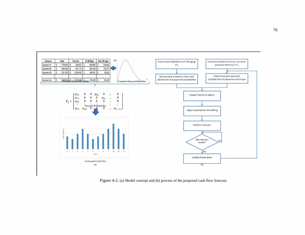
76
Figure 4-2. (a) Model concept and (b) process of the proposed cash flow forecast.

77
The first step is to define the Markov chain states in order to prepare a transition matrix
to calculate the cash flow forecast. To formulate the Markov Chain, the transient states and the
absorbing states are defined from the accounts receivable aging. Let St = [0, 1, 2, …, n] be a set of
transient states where 0, 1, 2, and n represent the AR aging states in the Markov Chain. Typically
in practice there are 4 states corresponding to 0-30 days, 31-60 days, 61-90 days, and over 120
days, as summarized in Table 4-1 below.
Table 4-1. State definition.
AR aging State
0-30 day 0
31-60 days 1
61-90 days 2
… …
Last AR aging range n
Additionally, two absorbing states are defined as Sa = [P, B] where P and B represent
Paid and Bad Debt states. An absorbing state is a Markov chain state, which can be reached from
any state. However, once it enters the absorbing state, it cannot leave this state. Table 4-2 shows
an example of the accounts receivable aging and defined states of the Markov chain in
parenthesis.

78
Table 4-2. Accounts Receivable Aging and Bad Debt.
Month Total Account Receivable Aging (state i)
(period j) Current 30days 60days 90days Over120days Bad debt
(0) (1) (2) (3) (4) (B)
November
(11)
1,609,405 702,560 623,810 101,470 36,480 127,085 16,270
December
(12)
2,655,895 1,418,250 530,080 528,400 75,295 103,870 12,328
January
(1)
2,287,070 896,140 505,465 669,020 76,330 140,115 4,556
February
(2)
2,109,595 829,995 586,160 450,745 66,365 107,700 13,590
The accounts receivable aging in Table 4-2 can be converted into the accounts receivable
aging matrix (R).
(4.1)
where is the amount of the accounts receivable aging in period j at State i and is the
amount of bad debt in period j.
Figure 4-3 shows the state transition diagram and the notation for corresponding
transition probabilities. The process starts from State 0, indicating the current charges (0-30 days)
in the AR aging, and transitions to State P if the invoice is Paid while in this state; or transitions
to State 1 (31-60 days) if the invoice is not paid. The probability of an invoice getting paid in
State 0 is modeled as the transition probability from State 0 to State P and denoted by p0P.
Therefore probability from State 0 to State 1 can be modeled as p01 = 1- p0P. The process

79
continues to the last state n where it can move to either State P (Paid) or B (Bad Debt). Since P
and B are the absorbing states, pPP = 1 and pBB = 1 in this model.
Figure 4-3. Markov chain state diagram.
Then determine the remaining 2(n+1) payment probabilities. Let PP be the (n+1)×2
matrix of the payment probability, which is the transition probability from any transient state n to
State P.
(4.2)
where is a weighting parameter, is the payment probability matrix from the AR aging and
is the payment probability matrix from the customer payment behavior. Here the payment
probability matrix is modeled to consist of two parts: the first part, models the aggregate
payment behavior across all customers of the firm in the recent past. This can be expected to
model any macro-economic trend that has influenced payment behavior across customers and
other trends across the industry. The second part, models payment behavior of a specific
customer at the individual invoice level based on all know payment history of the customer.

80
The weighting parameter can be obtained from back testing using historic data of
individual customers. The value of is selected to provide the most accurate forecasting result.
Furthermore, may vary from customer to customer, and over time. For a new customer, when
there is no payment history, would be set to unity thereby treating the customer as a “typical”
customer. However, for a longstanding customer, could be smaller thereby increasing the
weight for customer-specific payment behavior. The proposed model in Eq. (4.2) can be viewed
as a convex combination of Corcoran’s model and Pate-Cornell et al.’s model. If = 1, Eq. (4.2)
becomes Corcoran’s model and if = 0, it becomes Pate-Cornell et al.’s model.
can be determined from the changes in the accounts receivable aging from the
previous period to the current period Corcoran, 1978.
(4.3)
where
(4.4)
(4.5)
where is the payment probability from State i to State P (Paid),
is the transition
probability from State n to State B (Bad Debt), , , , and are the elements from
the accounts receivable aging matrix ( ) in Eq. (4.1).
models aggregate behavior across all customers of the firm, however, it does not
include customer specific payment behavior. Therefore, the second step, taking these factors from
distinct customers into account by modeling can be expected to improve the forecasting
accuracy. Assume that information of the customer payment behavior such as the number of days

81
that the invoices have been sent out to customers and the minimum number of days that
individual customer makes a payment are available.
(4.6)
To compute the probability of a given invoice that will be paid between time t0 and t0 +
∆t, the distribution of the payment time of each customer can be modeled conveniently as
Weibull distribution (Pate-Cornell, 1986; Pate-Cornell et al., 1990).
Figure 4-4. Weibull distribution with the shape parameter k = 1, 2, and 5, respectively.
Figure 4-4 shows Weibull distribution with the scale parameter = 1 and the shape
parameter k = 1, 2, and 5, respectively. Notice that for the shape parameter k = 2, this particular
distribution provides a linearly increasing rate, which rises to a peak quickly and then decreases
over time. This model of individual customer payment behavior can be used to characterize
payment lead-time that is used to set payment terms, probability of payment delay beyond the
expected lead-time, and probability of bad debt. In this dissertation, individual customer is
modeled using a Weibull distribution with the shape parameter k = 2

82
(4.7)
where is the scale parameter.
The probability that an invoice will be paid during time t0 + ∆t can be written as
where is the payment probability from the customer payment behavior of State i, is the
time a given invoice is billed to the customer, and is the cumulative distribution for the
payment time of the accounts receivable. From the cumulative distribution function, we can
determine three possible cases of the payment probability.
Case I:
(4.8)
Case II: and
(4.9)

83
Case III:
(4.10)
where is the minimum payment time and is the estimate scale parameter which characterizes
customer's payment lead time (Pate-Cornell et al., 1990). These model parameters can be
estimated periodically or even after invoice payment.
Once the payment probabilities and
are obtained, can be determined by Eq.
(4.2) and then , the (n+1) square matrix of the delay payment probability, can be determined
by
where
(4.11)
is the probability of the amount that will age from State i to State i+1 and is the
payment probability from matrix . Now it is ready to construct a transition matrix for period j,
Tj, from the probabilities in step 1 and step 2 as shown in Eq. (4.12).
(4.12)

84
Then, we use an exponential smoothing technique to smooth the data and then perform the
forecast of the next period cash flow. The formula of the exponential smoothing technique can be
written as
(4.13)
where
is the estimated transition matrix or exponentially smoothed matrix for period j
is the smoothing factor
is the transition matrix for period j
The smoothing factor can be identified by back-testing historic data of a firm to
provide the most accurate forecast.
Then, the cash inflow forecast and bad debt can be obtained by Corcoran, 1978;
Tangsucheeva et al., 2013
(4.14)
where
is the forecast vector of dollar amount in each state for period j+1
is the vector of actual accounts receivable aging report in period j from matrix R
The final step checks the updated actual payment in order to update the payment
probabilities and then repeat Step 2 through 6 to dynamically update the cash flow forecast. This

85
individual customer payment forecast is repeated for all customers with outstanding invoices to
compute the firm level forecast.
4.3 Enterprise Level Application
To illustrate the application of the proposed model, we use AR aging data from a small
manufacturing firm in Pennsylvania, which is shown in Table 4-2 along with states of the Markov
chain in parenthesis. For the sake of simplicity, assume that the firm needs a close attention to a
particular customer. Based on the past payment history in 5 months of this customer, the average
payment time is 25 days and the minimum payment time that this customer pays his invoice is 20
days. This individual customer is modeled by fitting the corresponding AR aging data to identify
the Weibull distribution parameters. By using Minitab, given the lowest AD (Anderson-Darling
Statistic) = 0.304 and the significant LRT P value = 0.000, Weibull distribution with a shape
parameter k = 2 is selected.
We follow the process presented in Section 4.2. First, define the Markov chain state from
the accounts receivable aging as shown in Table 4-2 and then convert it to a matrix R as shown
below.
Then, determine the first part of the probabilities of the next payment, , using Eq. (4.3) and Eq.
(4.4).

86
= (896,140-586,160)/896,140 = 0.3459
Continue in the same manner to determine the rest of the payment probabilities, the transition
probabilities of State i to State P (Paid), for i = 0, 1, 2, 3, 4. Use Eq. (4.5) to determine the
probability of bad debt.
=13,590/140,115 = 0.0970
To determine the second part of Eq. (4.2), , the scale parameter of the Weibull
distribution must be determined first. Let X be the random variable of the payment time in the
Weibull distribution. The mean of this distribution for the shape parameter k = 2 can be
determined by
Hence, an estimate of scale parameter can be obtained as follows:
where is an estimate of scale parameter , is an average of the n past observations of
the payment time of the customer, and is the minimum payment time. Based on the given
information, the scale parameter of the Weibull distribution is

87
Given that the invoice was sent out to the customer 27 days ago and = 3 days,
which is 20 days, the probability of receiving the payment from this customer is
determined by Eq. (4.8) as follows:
Hence, the payment probability from State 0 to State P and the probability of the invoice will be
postponed to the next aging can be obtained from Eq. (4.2) and Eq. (4.11), respectively.
The weighting parameter = 0.2 is obtained from back testing using historic data of a
firm. Once and are obtained, next, repeat the processes to determine probabilities for
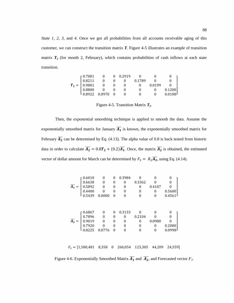
88
State 1, 2, 3, and 4. Once we got all probabilities from all accounts receivable aging of this
customer, we can construct the transition matrix T. Figure 4-5 illustrates an example of transition
matrix T2 (for month 2, February), which contains probabilities of cash inflows at each state
transition.
Figure 4-5. Transition Matrix T2.
Then, the exponential smoothing technique is applied to smooth the data. Assume the
exponentially smoothed matrix for January is known, the exponentially smoothed matrix for
February can be determined by Eq. (4.13). The alpha value of 0.8 is back tested from historic
data in order to calculate . Once, the matrix is obtained, the estimated
vector of dollar amount for March can be determined by , using Eq. (4.14).
Figure 4-6. Exponentially Smoothed Matrix and , and Forecasted vector F3.

89
The estimated vector F3 forecasts that the firm will have $1,580,481 collected cash from
the accounts receivable and $8,358 in bad debt whereas the actual cash collection and bad debt
are $1,540,900 and $6,275, respectively. Figure 4-6 illustrates Matrix , Matrix , and the
forecasted cash collection as well as bad debt. The difference of the cash collection between the
forecast and the actual value of the whole year is 2.31% whereas the difference of the bad debt is
14.79%. (We do not have information of detailed bad debt, so, we will not focus on the bad debt.)
Figure 4-7. Forecasting accuracy and and value.
Figure 4-7 shows relationship among forecasting accuracy, the smoothing factor, and the
weighting parameter . and are back tested from historic data: AR aging and customer
specific payment behavior. The selected values are chosen from the ones that provide the most
accurate average forecasting accuracy, which in this example, = 0.8 and = 0.2.

90
(1)
(2)
(3)

91
(4)
Figure 4-8. Sensitivity analysis of and for quarter 1, 2, 3, and 4.
Figure 4-8 shows the sensitivity analysis of how the forecasting accuracy changes over
and values for this specific customer. First observation is the highest forecasting accuracy of
each quarter is in the range of between 0.7 and 0.9 and in the range of between 0.1 and 0.3.
Since these parameters are quite sensitive to customer payment behavior, for the best of and
value, they can be varied from industry to industry, customer to customer, and time to time. If the
past data shows that and do not change with time then these parameters can be estimated
infrequently. Second, value is the exponential smoothing factor of the forecasting. The larger of
the is, the more weight on the most recent data is used to calculate the forecast. When
provides high forecasting accuracy, it implies that the payment behavior of this customer changes
significantly from its past payment. Therefore, using the outdated data or the further past data
may decrease the forecasting accuracy. Third, for this customer, the forecasting accuracy is
higher when value decreases. This implies that the payment behavior of this customer is quite
different from those of other customers. In other words, when , the payment behavior of
this customer is distinct from prevailing industry practice. Since the proposed forecasting model
is a convex combination of Corcoran’s model and Pate-Cornell et al.’s model, when , the

92
proposed forecasting model relies more on Pate-Cornell et al.’s model which incorporates
customer specific payment behavior. On the other hand, when , the proposed model relies
more on Corcoran’s model, which represents the aggregate customer behavior.
Let us consider another customer, customer #1, to see how the proposed model performs
the forecasting. This customer makes approximately 31 transactions on average per month. The
average payment time of this customer is 73 days and the minimum payment time is 48 days.
Table 4-3 shows the actual cash flow compared with the forecasted cash flow, and the percent
difference between the actual and the forecasted cash flow determined by five models: (1) the
proposed model, (2) Corcoran’s model to forecast cash flow from the accounts receivable aging,
(3) Pate-Cornell's model, (4) the moving average technique, and (5) the exponential smoothing
technique. For the proposed model, we extracted the accounts receivable aging of this customer
and followed the process mentioned in Section 4.2 to forecast the cash flow corresponding to this
customer. For Corcoran’s model and Pate's model, please see detailed explanation in Corcoran,
1978, and Pate-Cornell et al., 1990, respectively. For the moving average technique, we use 3
periods moving average to estimate the cash flow. Finally, for the exponential smoothing
technique, the smoothing factor is assigned to 0.8.
Table 4-3. Cash Flow and Forecasting Difference of Customer #1.
Month
Actual
Cash
Flow
($)
Proposed Model Corcoran’s Model Pate-Cornell's Model
Moving Average Exponential Smooth
Forecast Difference Forecast Difference Forecast Difference Forecast Difference Forecast Difference
($) (%) ($) (%) ($) (%) ($) (%) ($) (%)
1 21,547 21,922 1.74 22,920 6.37 24,890 15.52 31,604 46.67 31,604 46.67
2 21,145 21,045 0.47 25,244 19.39 21,679 2.53 26,576 25.68 23,558 11.41
3 50,890 50,616 0.54 36,974 27.35 45,018 11.54 24,765 51.34 21,627 57.50
4 56,767 59,468 4.76 60,752 7.02 67,564 19.02 31,194 45.05 45,037 20.66
5 43,881 43,506 0.85 50,029 14.01 54,883 25.07 42,934 2.16 54,421 24.02
6 44,776 43,634 2.55 48,354 7.99 42,664 4.72 50,512 12.81 45,989 2.71

93
Figure 4-9. Cash flow from actual cash flow and various forecasting models.
Figure 4-9 illustrates how a customer’s actual cash flow changes during month 1 through
month 6 compared to 5 other cash flow forecasting models. This figure shows how well the
forecasting models can keep track of the actual cash flow. While the cash flows forecasted by the
moving average technique and the exponential smoothing technique have some time lag to follow
the change of the actual cash flow, Corcoran’s model and Pate's model do not have this issue.
Thus, they can keep track the actual cash flow better than the former two models. However, they
still cannot keep track of the sudden change since the model determines the payment probability
based on only previous payment regardless of customer payment behavior. Consequently, when
the next payment drastically changes, the estimation from Corcoran’s model and Pate's model
have big gaps. On the other hand, the proposed model takes the customer payment behavior into
account. It considers the average payment time and the minimum payment time of the customer
to calculate the payment probability. Hence, the proposed model is able to keep track of the actual
cash flow as if they are the same line.
0
10
20
30
40
50
60
70
80
1 2 3 4 5 6
$ T
ho
usa
nd
Month
Actual Cashflow Proposed Model Corcoran's Model
Pate's Model Moving Average Exponential Smoothing

94
Figure 4-10. Percent difference of forecasting models.
Figure 4-10 depicts percent difference between the actual cash flow and the forecasting
models. As shown in the figure, the propose model has the smallest difference among four
models followed by Corcoran’s model.
Figure 4-11. Average percent monthly difference.
0
10
20
30
40
50
60
70
1 2 3 4 5 6
% D
iffe
ren
ce
Month
Proposed Model Corcoran's Model Pate's Model
Moving Average Exponential Smoothing
0
5
10
15
20
25
30
35
Proposed Model
Corcoran's Model
Pate's Model
Moving Average
Exponential Smoothing
% A
vera
ge D
iffe
ren
ce (
Mo
nth
ly)

95
Figure 4-12. Accumulated percent annually difference.
Figure 4-11 and Figure 4-12 show forecasting performance of each forecasting model on
an average monthly basis and average annually basis, respectively. In Figure 4-11, the proposed
model performs the best with approximately 3% difference on average while the difference from
Corcoran’s model and Pate's model are almost 15% on average, and the differences from the
moving average and the exponential smoothing technique are approximately 30% on average.
The percent difference of the last two models is relatively a lot larger than that of the proposed
model since these two models use only the average values from the historical data to smooth out
fluctuation. This is why these two models cannot capture the change of the actual cash flow in a
timely manner.
The accumulated differences shown in Figure 4-12 are, of course, smaller than those in
Figure 4-11 since the overestimate and underestimate are offset. Still the results shown in Figure
4-12 are consistent to those shown in Figure 4-11, the proposed model still performs the best
among these five methods.
0
2
4
6
8
10
12
14
Proposed Model
Corcoran's Model
Pate's Model
Moving Average
Exponential Smoothing
% A
ccu
mu
late
d D
iffe
ren
ce(A
nn
ual
ly)

96
Figure 4-13. Forecasting differences (monthly).
Next, the experiment was conducted to five sample customers over 12 months, who have
different payment behavior, to see how the forecasting models perform in different scenarios. In
this case, the customers have different number of days in accounts receivable, average payment
time, and minimum payment time. Customer #1 represents customers who have an average
payment time longer than 60 days with = 0.8 and = 0.2, customer #2 and customer #3
represent customers who have an average payment time approximately between 45-60 days with
= 0.6 and = 0.3, customer #4 and customer #5 represent customers who have an average
payment time approximately 31-50 days and less than 30 days with = 0.9 and = 0.1,
respectively.
Figure 4-13 shows the differences of the five forecasting models compared to the actual
cash flow of each customer. The proposed model still performs the best by providing the smallest
difference among five forecasting models. The percent difference of the proposed model on
average from five customers is approximately 6% while the percent differences of the other
models are much greater as shown in Figure 4-14. The proposed model is able to adjust the
parameters relating to the payment behavior so that it can manage to keep the gap of the
Proposed Model
Corcoran's Model Pate's Model
Moving Average Exponential Smooth
0
100
200
300
400

97
difference small compared to other models, which do not have this parameters involve in the
forecast.
Figure 4-14. Average forecasting difference (monthly).
Notice that the difference of the moving average and the exponential smoothing
techniques of customer #3 and customer #4 are large because there is so large fluctuation at some
points in time that these two models create big gaps between the actual cash flow and the
forecasted cash flow.
0
20
40
60
80
100
120
140
Proposed Model
Corcoran's Model
Pate's Model
Moving Average
Exponential Smooth
% A
vera
ge D
iffe
ren
ce (
Mo
nth
ly)

98
Figure 4-15. Forecasting difference (annually).
Figure 4-15 and Figure 4-16 show the performance of the five forecasting techniques in
aggregated level (annually). The results here are still consistent with the results of the monthly
basis shown in Figure 4-13 and Figure 4-14. The forecasting models perform better because of
the aggregated amount offset. The proposed model performs the best among five methods with an
average of approximately 4% different from the actual cash flow while Corcoran’s model has a
difference of approximately 9%, Pate's model has a difference approximately 7%, the moving
average technique has a difference of approximately 25%, and the exponential smoothing has a
difference of approximately 15%.
Proposed Model
Corcoran's Model Pate's Model
Moving Average Exponential Smooth
0
20
40
60
80
Customer #1
Customer #2
Customer #3
Customer #4
Customer #5

99
Figure 4-16. Average forecasting difference (annually).
4.4 Supply Chain Level Application
This section discusses how the proposed model performs in the supply chain and how it
is impacted by one of the most common problems in supply chain, the bullwhip effect. The
following section defines the bullwhip effect (BWE), the inventory bullwhip (IBW), and the cash
flow bullwhip (CFB), respectively.
4.4.1 Bullwhip Effect (BWE)
One of the bullwhip effect models that is widely accepted was developed by Chen et al.,
2000. The model starts with a simple supply chain, which contains a single manufacturer and a
single retailer. The customer demand is in the form of Kahn, 1987
(4.15)
0
5
10
15
20
25
30
Proposed Model
Corcoran's Model
Pate's Model
Moving Average
Exponential Smoothing
% A
vera
ge D
iffe
ren
ce (
An
nu
ally
)

100
where d is a nonnegative constant, ρ is a correlation parameter satisfying |ρ|<1, and μt is an
independent and identically normally distributed random variable with zero mean and variance σ2.
Assume the lead time L is fixed and the order-up-to policy is applied; hence, the order quantity
(qt) can be written as
(4.16)
where is the order-up-to point which is estimated from the observed demand as
(4.17)
where is an estimate of the mean lead time demand using a simple moving average, z is a
constant to meet a desired service level, and is an estimate of the standard deviation of the L
period forecast error. The bullwhip effect of a simple supply chain can be obtained from the
following (Chen et al., 2000):
(4.18)
The bound is tight when z = 0.
More detail of this model is discussed in Chen et al., 2000.
4.4.2 Inventory Bullwhip (IBW)
From the previous section, the inventory bullwhip model is extended to see how the
bullwhip effect impacts the inventory. For a simple supply chain containing a single retailer and a

101
single manufacturer, the lower bound of the inventory bullwhip can be written as Tangsucheeva
and Prabhu, 2013
(4.19)
where I is inventory level. The bound is tight when z = 0.
(4.20)
More detail of this model has been discussed elsewhere in Tangsucheeva and Prabhu,
2013.
4.4.3 Cash Flow Bullwhip (CFB)
The model above is further extended for the cash flow bullwhip in order to determine the
effect of the bullwhip effect and the inventory bullwhip to the cash flow (Tangsucheeva and
Prabhu, 2013). CFB is the variance of the cash conversion cycle (CCC) over the variance of
demand. CCC is the most widely used measurement for cash flow. It contains inventory (days
inventory outstanding), cash inflow (days sales outstanding), and cash outflow (days payable
outstanding) and this is the reason why CCC is used to represent the cash flow.
CFB for a simple supply chain can be obtained from the following formulae
(Tangsucheeva and Prabhu, 2013):

102
Case I: D ≤ I
(4.21)
Case II: D > I
(4.22)
where s is the sales price per unit, c is the unit cost, E(D) is the expected value of demand, and
E(I) is the expected value of inventory.
Further information regarding to this model is presented in Tangsucheeva and Prabhu,
2013.
4.4.4 Simulation Model
A supply chain simulation is one of a powerful and widely used tool for supply chain
analysis. Particularly, in case the analytical model cannot provide a clear analysis or stochastic
nature exists in the supply chain. Therefore, in this study, simulation experiments are developed
for the purpose of analyzing the cash flow forecasting accuracy at different stages of supply chain
and at different intensity of bullwhip effect.

103
4.4.4.1 Simulation Structure and Process
A simulation model of a multi-stage supply chain contains a single supplier, three
manufacturers, three distributors, and three retailers. Its structure and product flow of the supply
chain are shown in Figure 4-17 while its cash flow is in the reverse direction of the product flow.
Originally, the simulation model was created for a simple supply chain, which contains only a
single member in each stage and then more members were added into the model for more
practical illustration. The supply chain members in each stage can be adjusted later for more
proper use in each supply chain.
Figure 4-17. Structure of a supply chain in this simulation.
A simulation starts from a customer demand obtained from Eq. (4.15) with a 0.5 demand
correlation. The customer demand is produced for 72 months including a 12 months warm up
period for each input variable and it is generated separately for each retailer in order to represent
three retail stores that have different customer demands. Assume that the initial inventory is twice
as much of the customer demand. Each retailer fills the customer demand and periodically
observes its inventory level. Excessive demand is backordered and will be filled first when the
inventory is replenished. By the end of the observation period t, it places an order to the
distributor to replenish its inventory level. The order quantity follows Eq. (4.16). A fixed lead
Supplier Manufacturer Retailer Distributor

104
time L is applied, thus, the order will be received at the start of period t+L and then the process
repeats. The supply chain process of the four members—retailers, distributors, manufacturers,
and a supplier—are treated in a similar way except that each manufacturer receives orders from
three distributors. The process continues like this through the upstream members. The simulation
runs for 2,160 days (72 months including the warm up period) for each different bullwhip effect
value (from BWE = 1 through BWE = 20) to observe the inventory bullwhip, the cash flow
bullwhip, and the cash flow forecast error at all different stages in supply chain. The simulation
model focuses on the material flow and the cash flow among supply chain members.
In order to obtain preliminary insights, some known sources of variability are reduced.
Therefore, in this simulation, all supply chain members apply the same moving average
forecasting method and the same order-up-to inventory policy as well as the same lead time
throughout the supply chain. Additional assumption is that the accounts payable and the accounts
receivable are 80% of total purchases and sales each period with a 30 days payment term,
respectively. However, not all accounts receivable is collected within the pre-determine payment
term. The uncollectible amount over 120 days in the accounts receivable aging is written off as a
bad debt.
4.4.4.2 Simulation Tool
This simulation model is developed by Visual Basic for Applications (VBA) in Microsoft
Excel 2007. The three main reasons why we use the VBA in Excel is that, firstly, the data
regarding to the inventory and the cash flow is mostly in the tabular form or spreadsheet.
Therefore, input and output variables in this simulation are easy to manage in Excel. Secondly,
Excel provides adequate capabilities for the required computations, statistical analysis, and chart
generation. Lastly, Excel is a very common program used in many companies. Therefore, it is

105
very practical to develop the simulation in Excel. Our simulation model has a friendly user
interface, which is easy to use and configure.
Tangsucheeva and Prabhu, 2013 shows that an increase in the bullwhip effect leads to an
increase in the inventory bullwhip (IBW) and the cash flow bullwhip (CFB). Adverse impacts
from these effects include inventory, cost, and cash flow management difficulty. These effects
also propagate upstream in supply chain the same way as the bullwhip effect. In other words, the
impact of these phenomenon is worse in upstream members, particularly the supplier
(Tangsucheeva and Prabhu, 2013).
In this section, five cash flow forecasting models are compared among others on the
increase of the bullwhip effect to see how they are impacted as shown in Figure 4-18. This
experiment was conducted in the simulation model, which contains a supplier, three
manufacturers, three distributors, and three retailers as mentioned in Section 4.4.4.1.
Figure 4-18. Comparison among five techniques at a manufacturer stage.
As the bullwhip effect increases, gaps of the differences between the actual cash flow and
the forecasted cash flow also increases leading to worse accuracy, except the proposed model.
Figure 4-18 shows that the result from the proposed model with = 0.8 and = 0.2 and the
0%
5%
10%
15%
20%
25%
30%
1 2 3 4 5 6 7 8 9 10 11 12 13 14 15 16 17 18 19 20
Cas
h F
low
Fo
reca
st D
iffe
ren
ce
Bullwhip Effect
Cash Flow Forecast (Monthly) Proposed model Corcoran's model Pate's model SMA SES

106
Pate's model are largely independent of the bullwhip effect. The gap of the difference between the
actual cash flow and the forecasted cash flow remains approximately the same. On the other
hand, the other three models perform the cash flow forecast based heavily on the historical data
only. Therefore, when the data contains large fluctuation, especially when the bullwhip effect is
large, it significantly impairs the forecasting accuracy. This is the reason why Corcoran’s model,
the simple moving average technique (SMA), and the exponential smoothing technique, have
their cash flow forecasting differences increase.
Figure 4-19. Cash flow forecast difference at different stages of supply chain (Moving average).
Figure 4-20. Cash flow forecast difference at different stages of supply chain (Proposed model).
0%
10%
20%
30%
40%
50%
60%
70%
80%
1 2 3 4 5 6 7 8 9 10 11 12 13 14 15 16 17 18 19 20
Cas
h F
low
Fo
reca
st D
iffe
ren
ce
Bullwhip Effect
Cash Flow Forecast (Monthly) Retailer Distributor Manufacturer Supplier
0%
1%
2%
3%
4%
5%
1 2 3 4 5 6 7 8 9 10 11 12 13 14 15 16 17 18 19 20
Cas
h F
low
Fo
reca
st D
iffe
ren
ce
Bullwhip Effect
Cash Flow Forecast (Monthly) Retailer Distributor Manufacturer Supplier

107
Figure 4-19 and Figure 4-20 break down the impact of the bullwhip effect on the cash
flow forecast to each supply chain level and compare the performance of the forecasting
techniques between the two models, the moving average and the proposed model with = 0.8
and = 0.2. To be easily distinguishable, the moving average technique is selected to compare
with the proposed model since it performs the worst among four models. As shown in Figure
4-19, the gaps of the forecasting differences from the moving average technique increase when
the bullwhip increases and this inaccuracy continues to amplify when moving upstream toward
the supplier. In the worst case scenario, when the bullwhip effect is very high (BW = 20), the
cash flow forecast of the supplier may approximately result in 70% deviate from the actual cash
flow. This effect can cause the supplier a huge amount of interest expense, working capital,
opportunity cost, and so forth, meanwhile the forecasted cash flow from the proposed model
remains about the same, under 2% for all supply chain levels.
4.5 Conclusions
The proposed cash flow forecasting model was developed to assist a firm to have
accurate results and be convenient to use since the model obtains input data from the accounts
receivable aging, which is one of the accounting routine the firm already has. The model is based
on the combination of the work done by Cyert et al., 1962, Corcoran, 1978, and Pate-Cornell et al
Pate-Cornell, 1986. The proposed cash flow forecasting for firms is developed by integrating two
models: (1) Markov chain model of the aggregate payment behavior across all customers of the
firm using accounts receivable aging and; (2) Bayesian model of individual customer specific
payment behavior at the individual invoice level.
Actual data from a small manufacturing firm in Pennsylvania was used as the empirical
study to evaluate the performance of the forecasting models. The experimental results were

108
generated by the calculation from the analytical models and from a series of simulations. The
overall performances of the proposed model were compared with the Corcoran’s model, Pate's
model, and other two common practice models, the moving average and the exponential
smoothing techniques, which are widely used in small and medium companies.
In summary, the proposed cash flow forecasting model was demonstrated to be a simple
and most accurate forecasting technique for the firm in comparison with other models. The
proposed model performs the best with approximately 3%-6% different from the actual cash flow
and approximately 2%-4% difference on an aggregate level. For the supply chain level
application, the proposed model was shown to be independent of the bullwhip effect. The
forecasting accuracy of the proposed model is high and seems to be largely robust to supply chain
dynamics, including when subjected to severe bullwhip effect whereas those of other models
become worse when the bullwhip effect is severe. Potential key impact of accurate forecast is
efficient management of working capital. By reducing the forecast error from 20% (using simple
moving average) to 2% we can reduce the cost of running a business, especially for suppliers who
are likely to be SME. In addition, the proposed model was developed in an Excel spreadsheet
format which links to the accounts receivable aging. This development provides users a practical
and convenient forecasting tool to use even for a person who is not familiar with cash flow
forecast.
Regarding the exponential smoothing factor and the weighting parameter , these two
parameters are back tested from the payment historic data and selected from best values, which
provide the highest forecasting accuracy. We found that these parameters are quite sensitive and
can vary from industry to industry, customer to customer, and time to time. Since the proposed
forecasting model is a convex combination of Corcoran’s model and Pate-Cornell et al.’s model,
when , the proposed forecasting model relies more on Pate-Cornell et al.’s model which
incorporates customer specific payment behavior. This implies that the payment behavior of this

109
specific customer is different from the others. A firm needs to pay close attention to any customer
that has because of its distinct from prevailing industry practice, especially when it is an
important customer. On the other hand, when , the proposed model relies more on
Corcoran’s model, which represents more aggregate customer behavior. The future direction of
this study could be dedicated to the testing of the depth of historic data, how far back of the data
we should go, exploit all data or just look one season back in order to determine the weighting
parameter .

110
Chapter 5
OPTIMAL PRICING WITH CONSTRAINTS ON WORKING CAPITAL
AND PAYMENT DELAY RISK
5.1 Introduction
Dynamic financial decisions are decisions concerning financial activities while a situation
and environment change over time leading to the change in financial decision-making. Such
decisions include allocating amount of funds to operate a firm, selecting projects and managing
their capital expenditure, financing both long-term and short-term, and managing working capital.
This dissertation focuses on a combination of allocating proper amount of investment in projects
within limited working capital and selecting projects that maximize profit and minimize credit
risk of a firm.
Allocating proper amount of investment in projects is similar to asset allocation problem
in financial investment strategy which diversifies investments in various categories of assets such
as stocks and bonds in order to balance risk and return. Similarly, a firm seeks to invest in
projects from several potential candidates, which have different profit and risk in order to balance
its risk and return corresponding to its objectives.
The problem of project selection has caught fully attention to many researchers in project
management and engineering management. Due to a complex decision-making process and
various types of problems, many quantitative and qualitative techniques for selecting projects
have been proposed over the last 50 years. Project selection problem is involved by several
critical factors such as the market conditions, raw materials availability, probability of technical
success, government regulations, etc. (Bard et al., 1988). Make-to-order (MTO) firms are a type
of firms that may involve in project selection frequently. MTO firms must select the projects they
decide to pursue from among numerous opportunities. Apparently, this is not a simple problem to

111
solve. Poor decision-making may incur the firms to enormously expensive cost, which
consequently affects profit and loss. Particularly, an MTO firm participating in bidding has to
deal with several decision-making for project selection and bidding competition.
The whole bidding process can be divided into four phases, which are acquisition of the
project information, pre-evaluation of the project (which project to bid), mid-evaluation (how to
bid), and implementation of the project as shown in Figure 5-1 (Wang et al., 2009). This
dissertation focuses on which projects to bid in the second phase, the pre-evaluation of the
project, of Figure 5-1.
Figure 5-1. Phase classification of design project bidding decision (Wang et al., 2009).
The process of project bidding decision begins with a need for a custom product from a
prospective customer. Then the customer identifies a number of qualified manufacturers, and
solicit proposals, or bids, to satisfy its requirements. On the bidder side, an MTO firm starts with
a detailed investigation of the project and then extensively collects and carefully reviews the
information of the tender project. This information includes specifications of the products and
Acquisition of the project information
Pre-evaluation of the project
(Bid/No bid and which projects to bid)
Mid-evaluation of the project
(How to bid)
Implementation of the project
Finish
Start

112
services corresponding to customer’s requirements (King and Mercer, 1988). MTO firms must
estimate all project requirements such as raw material, labor, time frame and completion time,
costs and working capital of the project and then tender their terms to meet the customer’s
requirements. Once all information is complete, the MTO firm is able to decide whether to bid or
not, which project to bid and how to bid, in order to develop a strategy to make an optimal bid for
projects.
On the other hand, the prospective customer also tries to have many options to select the
best one. Therefore, the customer usually solicits proposals to several different suppliers or
manufacturers and compares their terms. Some of the competing MTO firms may be invited to
submit bids for other jobs as shown in Figure 5-2. Therefore, not every bid submitted by an MTO
firm is likely to be successful. Finally, the project is awarded to a single bidder. The risk of the
MTO firm is that it may lose the biding competition to another competitor. According to the
survey of Tobin et al., 1988 about the bidding competition in UK, it shows that the proportion of
successful tendered bids that become orders of the firms is very varied between 3% and 100%.
The success of a bidding competition may depend on many different aspects, but bidding price is
frequently an important key to win the bid. Kingsman et al., 1989 identifies that bidding price
plays an important and critical role in winning or losing bid. Dempsey’s survey reveals that price
is among the top three factors with delivery capability and quality, which influence industrial
purchase decisions (Dempsey, 1978). Similarly, Dickson, 1966 findings show that there are 22
other important factors which customers evaluate during the selection process. These factors
include good quality and reliable delivery. Understand how these factors interact and affect each
other allows firms to construct the bidding strategies to win the bid. Once the customer decides
which bidder is a winner, occasionally, it may initiate negotiations with the bidder for more
favorable terms. Each stage of the bidding process may involve a considerable time lag (Slatter,
1990).

113
Figure 5-2. Scenario diagram of the MTO firm bidding.
The ultimate goal of MTO firms to participate in the bidding competition is not only to
win the bid, but also to earn profit for themselves. An MTO firm may win a bidding competition
with an unrealistically low price or delivery terms; as a result, this may risk the firm to earn so
low revenue that it cannot cover overall costs and eventually loss a profit – a phenomenon
sometimes called “the winner’s curse”. Friedman, 1956 and Gates, 1967 proposed bidding
strategies that manage bidding prices to maximize expected profits. Berkson’s binary choice logit
model was among the pioneers to apply an S-shape multi attribute model for choice probabilities
(Berkson, 1953). Later on, Easton and Moodie, 1999 included the lead time to deliver the project
to the S-shape logistical response function (logit model) to provide the winning probability of the
bidding competition. To optimize the expected benefits from a bidding competition, MTO firms
need to understand the relationship among prices, revenues, expenses, winning likelihood, and
return and risk.
MTO Firm
Project n
Project 1
Project 2
Project 4 Project 3
Competitor Competitor
Competitor
Competitor Competitor
Competitor
Competitor
Competitor
Competitor
Competitor
Competitor
Competitor
Competitor
Competitor

114
Default risk, a possibility of a default payment, is one of many problems MTO firms
encounter after deliver complete projects. Therefore, credit risk assessment and risk
compensation are also necessary for MTO firms to evaluate their customers. Credit risk refers to
the risk that a customer will default on its payments. The risk includes lost in
principal and interest, disruption to cash flows, and increased collection costs. The loss may be
complete or partial and can arise in a number of many possible circumstances. Credit risk also
leads to cash flow and working capital problem. To compensate this risk, additional amount
called default premium or risk premium can be added into bidding price.
Typically, the process of setting a bidding price of MTO firms is to evaluate all
associated costs and using a standard mark-up approach (Kingsman et al., 1993; Wisner and
Siferd, 1995). Mark-up is the additional amount that a firm adds to its estimated total costs for the
project to cover overhead, unplanned expenses, and desired profit (Ahmad and Minkarah, 1987).
Many literature in the competitive bidding focuses on these key decision variables (King and
Mercer, 1988). To construct an optimal bidding strategy, it is important that a firm realizes and
understands its objectives clearly since there are many possible objectives in a real business world
such as maximizing profit, minimizing loss, minimize profits of competitors, and just obtaining
the contract to keep production going even at a loss (Friedman, 1956). Different strategies are
required based on different objectives of the firms.
In what follows we first explains the analytical models of how the integer programming
is formulated in order to determine the combination of the project investment that maximize
profit and minimize credit risk in Section 5.2. Then, Section 5.3 describes the setup of the
problems and illustrates industrial case numerical examples. This section shows how the model
can be applied to the project selection problem. Then, the results and discussion are addressed in
Section 5.4. Lastly, in Section 5.5 the conclusion and direction for future work are discussed.

115
5.2 Pricing Model
This section we identify a potential strategy to engineer a solution for maximizing profit
and minimizing credit risk by using integer programming model. In practice, financial problems
involve multiple objectives that are dependent on the complex financial and nonfinancial
relationships that define the problem. The objective of this section is to apply an integer
programming model to this project selection problem.
To formulate this integrated project selection problem, credit risk minimization, and
working capital maximization, an integer programming approach is applied to determine an
optimal investment strategy. We will start with the objective functions. The first objective is to
maximize the expected profit.
5.2.1 Objective Functions
Expected Profit
In our problem, the uncertainty associated with the bidding is represented by a chance of
winning a bid. Let represent the probability that a bid of will be the lowest and win the
project, represent the amount of actual profit obtained from each selected project i in period j.
Then the expected profit, , if a bid of wins, can be written as
(5.1)
where the probability of winning bid can be obtained from Friedman (1965). Presumably
the results of previous bidding on contracts are always announced, and from these announced
bids the 'bidding patterns' of potential competitors may be studied. Additionally, each competitor

116
is likely to bid as he has done in the past, which is the best assumption in the absence of
additional information
(5.2)
where is the estimated number of bidders, is the cost of the project i in period j, a and d are
constants obtained from curve fitting frequency data to the gamma distribution. A gamma
distribution is a good fit to this sort of data, the probability density function of the ratio of the
average bidder’s bid to the firm cost estimate. The actual profit can be obtained from
(5.3)
where is the bidding price and is the cost of the project i in period j. Note that the cost
already includes both fixed cost (i.e. production set up cost and overhead) and variable cost (i.e.
unit cost and holding cost) of project i. The bidding price can be calculated by
(5.4)
where is the required percent markup of a firm and is the percent of the risk premium of
the project i in period j. Therefore, the actual profit can be rewritten as
(5.5)
Finally, the first objective function, maximizing the expected profit, can be written as

117
(5.6)
where is the binary 0-1 decision variables of the project i in period j where = 1 if the
project is selected and = 0 otherwise.
5.2.2 Constraints
Credit Risk
Tangsucheeva and Prabhu, 2014 proposes a stochastic analytics model to forecast cash
flow by building on the work done by Cyert et al., 1962; Corcoran, 1978; Pate-Cornell et al.,
1990. A part of this proposed model applies Bayesian technique to take customer specific
payment behavior into account to calculate the payment probability. By modeling the distribution
of the payment time of each customer as Weibull distribution with scale parameter = 1 and the
shape parameter k = 2, the probability of a given invoice that will be paid between time t0 and t0 +
∆t can be computed as follows:
Case I:
(5.7)

118
Case II: and
(5.8)
Case III:
(5.9)
where is the payment probability from the customer payment behavior (the transition
probability from the last state, State n, to State P (Paid) in the accounts receivable aging), is
the time a given invoice is billed to the customer, is the minimum payment time and is the
estimate scale parameter which characterizes customer's payment lead time (Pate-Cornell et al.,
1990). These model parameters can be estimated periodically or even after invoice payment.
Generally, if the invoice ages over the last State n in the accounts receivable aging, for
instance, 120 days, this invoice is usually written off as a bad debt in accounting. Hence, the
complement of , which is
, is the transition probability of State n to State (B)
Bad Debt within days. In other words, it is the probability of default payment. Therefore, the
probability of default becomes
Case I:
(5.10)

119
Case II: and
(5.11)
Case III:
(5.12)
To compensate these credit risk or default risk, we need to determine risk premium.
Typically, risk premium in the financial investment can be calculated by
where is the return of a risky asset such as stock and is the return of the risk-free asset such
as T-bill.
However, in the trade credit, the concept of the risk and return is different from that of
the financial investment. Risk premium in the trade credit can be determined by
where is the return from cash trade, which represents the return from the risk-free asset, and
is the expected return from the trade credit and can be determined by

120
where is the average payment probability of a customer within the payment term (depend on
the payment term i.e. 45 days, 60 days, 90 days, etc.).
Generally, in financial investment, the higher risk you invest in assets, the higher return
you get from them. However, this is not the case for the trade credit. Trade credit may expose to
credit risk or risk from delay payment whereas the cash trade does not have these kinds of risk
since the latter case a firm receive payment before or on delivery. Nonetheless, trade credit is
essential for business to business (B2B) sellers since it is one of several tools to attract buyers in a
competitive market.
However, the previous equation does not include the impact from the payment delay.
Therefore, taking time value of money into account, the risk premium for trade credit can be
rewritten as
where i is the required rate of return of a firm and n is the period of the delay payment. Finally,
the percent risk premium can be obtained from
(5.13)
The financial risk associated with this project bidding under uncertainty of the trade
credit is credit risk. It is defined as the risk premium which compensates the default risk.
(5.14)

121
where is the risk premium of the project i in period j and represents the maximum risk the
firm can expose to.
Machine Utilization
The sum of machine utilization of all selected projects must not exceed the total machine
utilization.
where is the expected machine gross utilization available based on all committed project i
in period j and U is the total machine utilization of the manufacturer.
Raw Materials
The amount of raw materials supplied by a supplier to various projects (to produce for
customers) at production facility, must be sufficient.
where is the total required amount of raw materials for the selected projects.
Labor
Labor or man-hour required for the selected projects must not exceed the total number of
maximum man-hours L.

122
where is the required number of hours for the selected projects and is the overtime hour for
the selected project must not exceed the maximum overtime O.
Storage Space
As occurs with the plants, it is defined a continuous variable in order to represent the
capacity of the warehouse or storage space. Therefore, the total inventory of kept at
warehouse during period j must be lower than the capacity of the warehouse. Warehouse space
must be sufficient.
where is the space required to store in the warehouse for the project i in period j.
Working Capital
Cash inflows and outflows are normally not synchronized, so that a positive cash balance
is required to operate the firm (Robichek et al., 1965). Lutz and Lutz, 1951 point out that the
synchronization of inflows and outflows might be improved, but at a cost. Capital budgeting,
Capital investment planning (limited capital and credit line). Each project requires the amount of
capital investment and the total capital investment must not exceed the available capital C.

123
Assume that C is the maximum working capital the firm can invest in selected projects. This
maximum working capital C is available for raw material cost, ordering cost, labor cost,
production cost, facilities cost (i.e. EE, gas, fuel, etc.), inventory holding cost, material handling
cost, G&A cost, overhead cost, and all other requirements for completing the selected projects.
These constraints are applicable to this empirical study. In practice, constraints can be
added or removed based on specific constraints of firms.
5.3 Industrial Case Numerical Examples
Two industrial cases, a firm with non recurring customers and a firm with recurring
customers, are presented in this paper. A small manufacturing make-to-order (MTO) firm in
Pennsylvania presented as a firm with non recurring customers has few standard products and
volatile. The second case is another manufacturing firm with recurring customers. For the MTO
firm, a production order usually stems from a successful bid. To participate in a bidding
competition, the MTO firm must estimate the resource requirements, the completion time, direct
costs of the project, and then tender its term to meet the customer’s requirements. The customer
may decide to accept, reject, or modify these terms. However, in this study, we assume that there
is no modification of these terms. Many of the important operational decisions that associate with
the MTO firm do not begin until a customer places an order. This scenario is not a mutually
exclusive, the company can select more than one project as long as all constraints are not violated
and all projects are independent. Periodically, the MTO firm has several projects to bid with

124
several different customers, but with a limited working capital. Each project provides different
profit and chance to win the bid, exposes to different level of credit risk, requires different
amount of working capital and capacity constraints.
The firm has a 30 days fixed payment term to its supplier in order to have an edge of low
raw material cost over its competitors. On the other hand, the payment term from its accounts
receivable may vary from 60-90 days assuming all projects are trade credit. Some customers pay
their invoices on time or before time while the others pay late. The accounts receivable that age
over 120 days are considered as a bad debt. These delay payments and default risk effect the
firm’s cash flow and working capital. The firm’s cash flow is forecasted by the stochastic
financial analytics model (Tangsucheeva & Prabhu, 2014). Thus, the firm knows its cash flow
and want to manage it efficiently. The firm can have a large amount of working capital sitting in
its account, but doing so, it may lose an opportunity to profit from excess cash. Meanwhile, too
little of working capital may risk the company to be insolvent and lose opportunity to profit from
investing in other projects.
Therefore, the challenge here for the firm to be decided is to select the projects which
maximize profits, minimize risk, and maximize working capital within a limited resources. The
firm may have to trade-off profit with risk and working capital with opportunity cost (excess
cash) and liquidity problem (cash shortage). These types of decisions repeat every period.
5.3.1 Industrial Case - Firm with Non Recurring Customers
To illustrate the model, we use actual cash flow data from a small manufacturing firm
where we know cash inflow and cash outflow. Thus, the next period working capital can be

125
forecasted. The problem consists of determining the optimal strategy to allocate working capital
to various projects in order to maximize profit and minimize credit risk.
In this illustration, we consider five potential project candidates. We consider a planning
horizon of 6 months. The process starts by estimating credit risk of customers. Most companies
typically write off the remaining balance (delinquent amount) after 120 days of accounts
receivable aging as a bad debt. is the payment probability of the outstanding balance that will
be paid within 91-120 days, hence, is the probability that this project will not get paid
within 120 days. In other words, it is the probability of the bad debt.
For customer #1, since the outstanding balance age, , is 91 days whereas the
average payment time is 95 days and the minimum payment time is 60 days, therefore, Eq.
(5.10) is used to calculate for Case I.
=0.1704
Then we are able to calculate the risk premium of this customer using Eq. (5.13) where
the required rate of return of a firm i is 20%.
Once we know the risk premium, we can determine the required minimum bidding price
and the actual profit if winning the bid, using Eq. (5.4) and (5.5), respectively, assuming

126
the required working capital investing in this project is $1M and the required percent markup
is 30%.
Next, to determine the expected profit , if a bid wins, apply Eq. (5.1) and Eq. (5.2)
assuming there are 10 bidders in this project, a and d are 2 and 10, respectively.
Repeat these steps to determine risk and return of other projects. Table 5-1 summarizes
parameters for determining risk and return of 5 projects to be considered in period 1.
Table 5-1. Objective function parameters.
Project Credit
Risk
Risk
Premium
Percent
Markup
Working
Capital
Minimum
Bidding
Price
Winning
Probability
Actual
Profit
1 0.1704 17.32% 30% $1,000,000 $1,473,200 99.75% $473,200
2 0.3210 32.64% 25% $700,000 $1,103,480 99.65% $403,480
3 0.5367 54.57% 30% $400,000 $738,280 99.23% $338,280
4 0.7295 74.17% 45% $1,500,000 $3,287,550 98.35% $1,787,550
5 0.8841 89.89% 30% $800,000 $1,759,120 93.42% $959,120
However, the purpose of a firm is not just to win the bid, but to make profit too. The
required minimum bidding price of a firm may not provide the highest expected profit. Thus, we
construct to vary the bidding price of Project 1 to see how the expected profit changes.

127
Table 5-2. Various bidding price vs expected profit.
Bidding Price ($) Expected Profit ($)
1,473,200 472,011
1,600,000 597,024
1,800,000 789,894
2,000,000 972,002
2,200,000 1,133,646
2,400,000 1,261,503
2,600,000 1,340,462
2,800,000 1,357,392
3,000,000 1,305,959
From Table 5-2, the bidding price at $2.8M provides the highest expected profit of
$1.357M with the winning probability of 75.41%. Table 5-3 shows the bidding prices which
provide the highest expected profit of 5 projects.
Table 5-3. Bidding prices and expected profits
Project Minimum
Bidding Price
Number of
Bidders
Bidding Price
providing
Highest
Expected Profit
Winning
Probability
Expected
Profit
1 $1,473,200 10 $2,800,000 75.41% $1,357,392
2 $1,103,480 8 $2,030,000 75.64% $1,500,986
3 $738,280 5 $1,240,000 77.32% $649,496
4 $3,287,550 3 $5,250,000 74.41% $2,790,424
5 $1,759,120 12 $2,160,000 76.32% $1,038,025

128
Table 5-4. Constraint parameters.
Project Machine
Utilization
Raw
Materials
(lbs)
Labor
(hrs.)
OT
(hrs.)
Storage
Space (ft2)
Working
Capital
1 0.2 3,800 3,200 960 3,600 $1,000,000
2 0.17 2,500 2,800 840 3,000 $700,000
3 0.10 2,000 2,400 800 2,500 $400,000
4 0.42 4,000 3,800 740 9,400 $1,500,000
5 0.23 3,200 3,000 700 4,300 $800,000
Table 5-5. Upper and Lower bound.
Machine Utilization Raw Materials
(lbs)
Labor
(hrs.)
OT
(lbs.)
Storage Space
(ft2)
Working Capital
0.95 10,000 10,000 2,500 20,000 ft2 $4,000,000
Table 5-4 and Table 5-5 summarize the constraints and upper and lower bound for integer
programming formulation. Once we know the optimal bidding price and maximum expected
profit for each pricing, then, from the data in Table 5-1 through Table 5-5, we can formulate the
integer programming model to determine which project combination provides maximum profit
and minimum risk.
5.3.2 Industrial Case - Firm with Recurring Customers
We also test the model with another small manufacturing firm which has its customers
constantly coming back for reordering. Even though there is no bidding competition in this
scenario, it is similar to the first scenario since the firm has to compete with its competitors
through pricing, assuming that price is the decision variable to convert the purchasing quotation

129
to the purchasing order. The objective of the firm is the same as that of the first scenario which is
to maximize profit and minimize credit risk. Therefore, pricing strategy plays an important role in
getting the order. The differences between these two scenarios are that the firm with recurring
customers is more familiar with its customers and customers’ payment behavior, therefore, it can
assess customers’ credit risk and hence forecast its cash flow more accurately.
We use the model to run the experiment to see how it works with this scenario. In this
illustration, five customers request the quotations from the firm and competitors of the firm. We
consider a planning horizon of 6 months. To formulate the integer programming, we follow the
same procedure as the previous section by starting to determine the price, calculating credit risk
and risk premium of these five customers, and then setting up the required percent markup as
shown in Table 5-6. Next we use Eq. (5.1) and Eq. (5.2) to determine the price which provides
the highest expected profit as shown in Table 5-7.
Table 5-6. Objective function parameters.
Customer Credit
Risk
Risk
Premium
Percent
Markup
Working
Capital
Minimum
Quote Price
Winning
Probability
Actual
Profit
1 0.2920 29.80% 25% $12,000 $18,577 99.88% $6,577
2 0.1536 15.68% 25% $15,000 $21,102 99.95% $6,102
3 0.3404 34.75% 25% $23,000 $36,743 99.85% $13,743
4 0.1867 19.06% 25% $18,000 $25,931 99.94% $7,931
5 0.3495 35.68% 25% $26,000 $41,777 99.85% $15,777

130
Table 5-7. Bidding prices and expected profits
Customer Minimum
Quote Price
Number of
Competitors
Quote Price
Providing
Highest
Expected Profit
Winning
Probability
Expected
Profit
1 $18,577 1 $98,800 74.60% $54,312
2 $21,102 3 $48,000 78.22% $25,812
3 $36,743 2 $80,500 74.41% $42,787
4 $25,931 4 $55,800 77.32% $29,227
5 $41,777 5 $78,000 77.43% $40,266
Then we list the constraints of 5 customers and upper and lower bound of the firm,
respectively, as shown in Table 5-8 and Table 5-9.
Table 5-8. Constraint parameters.
Customer Machine
Utilization
Raw
Materials
(lbs)
Labor
(hrs.)
OT
(hrs.)
Storage
Space (ft2)
Working
Capital
1 0.12 1,700 1,600 300 2,500 $100,000
2 0.14 2,200 1,800 300 2,800 $100,000
3 0.17 3,500 2,100 900 4,800 $100,000
4 0.15 2,800 1,900 600 6,000 $100,000
5 0.20 4,300 3,000 900 7,000 $100,000
Table 5-9. Upper and Lower bound.
Machine Utilization Raw Materials
(lbs)
Labor
(hrs.)
OT
(lbs.)
Storage Space
(ft2)
Working Capital
0.80 13,000 10,000 2,500 20,000 ft2 $100,000

131
Then we are ready to formulate the integer programming model where is the binary 0-
1 decision variables of the customer i in period j where = 1 if the customer is selected and
= 0 otherwise.
5.4 Results and Discussion
We consider 5 projects for the project bidding competition scenario and 5 customers for
the purchasing quotation of recurring customer scenario in 6 periods time horizon. The model
was solved by LINDO on a Window 8 based Dell workstation with Intel Xeon 3.6GHz dual
processor. The model was terminated after 4 second of CPU time. Table 5-10 shows that for the
first scenario Project 2, 4, and 5 are selected to invest in this period with the expected profit of
$5.3M and credit risk of 1.967 within a $3M working capital. For the second scenario, Customer
1, 2, 3, and 5 are selected in this period with the expected profit of $163k.
Table 5-10. Results.
Results
Bidding competition Purchasing quotation
Selected Projects/Customers 2, 4, and 5 1, 2, 3, and 5
Expected Profit $5,329,435 $163,177
Credit Risk 1.967 1.136
Working Capital $3,000,000 $76,000
For the analysis part, since two scenarios provide similar results, we present only the
bidding competition scenario. Figure 5-3 (a) and Figure 5-3 (b) show the winning probability
among 10 bidders on Project 1 and the bidding pattern of 10 bidders in this bidding competition,
respectively. The winning probability is very high and is almost 100% chance of winning the bid

132
at the low price-cost ratio (PC ratio) range of 0.1 to 1.7, and then it drops sharply when PC ratio
increases over 2.0. Eventually, the winning probability drops to almost zero chance at the PC
ratio over 5.0.
(a)
(b)
Figure 5-3. Winning probability (a) and Bidding pattern of average bidder (b).
Figure 5-4 shows the expected profit of Project 1 over the PC ratio. At the beginning, the
expected profit is negative (loss) until the PC ratio increases over 1.0, then the firm starts to make
a profit. The expected profit keeps increasing quite linearly and reaches its peak of $1.36M at the
PC ratio of 2.8, and then it starts to decrease.
0
0.2
0.4
0.6
0.8
1
1.2
0 2 4 6 8 10
Win
nin
g P
rob
abili
ty
Price/Cost
0
0.05
0.1
0.15
0.2
0.25
0.3
0 2 4 6 8 10
Pro
bab
ility
Price/Cost

133
Figure 5-4. Expected profit over Price-Cost ratio (PC ratio).
Figure 5-3 (a) and Figure 5-4 show that the firm does not have much profit or even loss
when the firm try to bid at a very low price (low PC ratio) in order to just to win the bid (low
price, high winning chance). Since the objective of the firm is not only to win the bid, but also to
maximize its profit, thus, bidding at the lowest price or at a low profit may not be the best
strategy in this case.
Figure 5-5 shows the relationship between the expected profit and credit risk of Project 1.
The expected profit increases at the beginning when the credit risk is low and it keeps increasing
until the credit risk is 0.3636. Then, the expected profit starts to fall. The expected profit increases
while the credit risk increases because the firm compensates this risk by adding the risk premium
into the bidding price. Hence, when credit risk increases, the risk premium increases and the
expected profit still increases. However, at one point, the increase in the risk premium is not
sufficient to compensate the rising of credit risk. Thus, at this point, the expected profit starts to
decrease. At the point where the risk premium is not sufficient to compensate the credit risk, the
firm may need to re-evaluate its risk premium to compensate the high credit risk.
From Figure 5-5 implication, consider two projects that have the same characteristics
such as profit and required production capacity, but the credit risks are different. One project has
the credit risk of 0.3636, which provides the highest expected profit due to the additional risk
(1.50)
(1.00)
(0.50)
-
0.50
1.00
1.50
0 2 4 6 8 10
Exp
ecte
d P
rofi
t (M
illio
ns)
Price/Cost

134
premium, and the other project has the credit risk of 0.25. The firm should select the former
project if the objective of the firm is to maximize its profit. Otherwise, the firm may choose the
latter project for lower credit risk.
Figure 5-5. Expected profit vs Credit risk.
Figure 5-6 illustrates the relationship between the winning probability and the risk
premium. As the risk premium increases, it reduces the chance of winning the bid since the risk
premium is added to the bidding price to protect from the credit risk.
Figure 5-6. Winning probability vs Credit risk.
-
0.10
0.20
0.30
0.40
0.50
0 0.2 0.4 0.6 0.8 1
Exp
ecte
d P
rofi
t (M
illio
ns)
Credit risk
0.92
0.93
0.94
0.95
0.96
0.97
0.98
0.99
1
1.01
0 0.2 0.4 0.6 0.8 1
Win
nin
g P
rob
abili
ty
Risk premium

135
Figure 5-7. Expected profit vs Winning probability.
Figure 5-7 depicts the relationship between the expected profit and the winning
probability. This figure shows the phenomenon called winner’s curse where the increase in the
winning probability may lead to the loss of the firm. The winner of the bidding competition may
not be able to make a profit from the project since the bidding price may be too low to offset the
cost.
Figure 5-8. Expected profit vs Working capital.
Figure 5-8 shows the relationship among the expected profit, working capital, and the
selected projects. We relax other constraints to see how the expected profit increases when the
firm has more working capital. The solid line shows the increase in the expected profit when the
working capital is increased. The horizontal color bar chart in the background represents the
(1.50)
(1.00)
(0.50)
-
0.50
1.00
1.50
0 0.2 0.4 0.6 0.8 1
Exp
ecte
d P
rofi
t (M
illio
ns)
Winning Probability

136
selected projects (Project #1 through Project #5) over the range of working capital. For example,
if the firm has $2M working capital, investing in Project #3 and Project #4 provides it the
maximum expected profit of $3.44M. If the firm obtains more working capital from its line of
credit to $4M, then investing in Project #1, Project #2, Project #4, and Project #5 gives it
maximum expected profit of $6.69M. This graph helps the management team to make a decision
conveniently and effectively.
Table 5-11. Results for 6 periods.
Period Working
Capital
Credit
Risk
Expected Profit
Selected
Projects
1 $3,000,000 1.9670 $5,329,435 2, 4, and 5
2 $3,000,000 1.5783 $5,473,020 1, 3, and 4
3 $4,000,000 1.5821 $6,120,323 1, 2, and 4
4 $4,500,000 0.9647 $6,783,705 2, 3, 4, and 5
5 $6,000,000 1.4581 $8,539,460 1, 2, 4, and 5
6 $6,000,000 1.8937 $8,152,905 1, 2, 3, and 5
Once the decisions are made, the firm follows the strategy from the investment model in selected
projects. Before the end of the period, the firm has to prepare for the bidding competition of the
next period using the cash flow forecast to estimate its working capital for the next period. The
objective functions remain the same, which are maximized profit and minimize credit risk.
However, the constraints may change over time. The process repeats like this each period. The
results for 6 periods are shown in Table 5-11.

137
5.5 Conclusions
The problem of project selection has been given fully attention in engineering
management. How to select the best project or portfolio for more benefits. Especially for a firm
with non recurring customers, an MTO firm, participating in a bidding has to deal with project
selection and bidding competition. The purpose of bidding is to earn a profit, not simply to win
orders. An MTO firm might win a competition with an unrealistically low price, hence, the
revenue does not cover its costs and eventually results in loss of the firm.
We have applied an integer programming model to the firms to select which projects it
should invest in for maximizing profit by applying a competitive bidding strategy of Friedman
(1956) to determine the appropriate bidding price. In addition, we also take the credit risk into
account in the objective functions in order to control the loss from payment delay and default risk
at the acceptable level of the firm. The probability of default payment is calculated to determine
the risk premium which is added to compensate the risk. The model treats diverse manufacturing
and financial constraints such as production capacity and working capital. Other constraints can
be added or removed depending on the project requirements.
The solution of a model is a combination of selected projects which tradeoff between risk
and return and could be a basis for strategies and options for management to maximize their
profit, minimize risk, and avoid liquidity problem. A detailed numerical case study also shows
that the firm should invest in which projects corresponding to the available working capital in
order to maximize the profit and minimize the credit risk. In addition, the results show that the PC
ratio has an inversely proportional relationship to the winning probability and the winning
probability has the inversely proportional relationship to the risk premium. That is the winning
probability of the bidding is very high at a low PC ratio and the winning probability starts to

138
decrease when the PC ratio increases. Therefore, at a very low bidding price, the firm has a very
high chance to win the bid.
Similar to the risk premium, the increase in risk premium leads to the decrease in winning
probability. Since the risk premium is added to the bidding price to compensate the credit risk,
thus, the price is increased and the winning probability is decreased. However, at a high winning
probability, the firm may not be able to make a profit due to the unrealistically low bidding price.
The results also show that at a specific bidding price, the firm obtains the highest expected profit.
As a result, the firm should bid at this price in case its purpose is to maximize the profit.
Lastly, the relationship between the expected profit and the credit risk is concave function
where the expected profit increases at the beginning, reaches its peak, and then starts to fall when
the credit risk keeps increasing. In case there are two projects that have the same characteristics
such as profit and required production capacity, but the credit risks are different. From the
expected profit and credit risk relationship, the firm can see which project provides how much
profit at a specific credit risk and select the project based on its need to maximize profit or
minimize risk.

139
Chapter 6
CONCLUSIONS AND FUTURE DIRECTIONS
This chapter concludes all of the work done in this dissertation and summarizes future
directions of this research.
6.1 Conclusions
In Chapter 3, we postulate that there can be a corresponding bullwhip in the cash flow
across the supply chain. The bullwhip effect is one of the most common problems found in
supply chain management. It not only has tremendous impact on supply chain efficiencies, but it
also has an impact on the cash flow in many ways. We successfully develop and analyze the cash
flow bullwhip model and find that the increase in the bullwhip effect results in the increase in the
variance of inventory and the cash conversion cycle, leading to the increase in the cash flow
bullwhip eventually. In addition, severe cash flow bullwhip takes place in upstream members
such as suppliers and manufacturers once the bullwhip effect propagates upstream to these
members.
We found that the cash flow bullwhip is an increasing function of the bullwhip effect and
the lead time, but it is a decreasing function of the demand observation period. This result
supports the idea that the large lead time and small number of moving average observation period
may produce the bullwhip effect. Once the bullwhip effect occurs, it causes the increase in the
variance of inventory and the cash flow bullwhip. In other words, since the amplified order does
not reflect the actual demand, which is lower than the order, therefore, the products will sit in the

140
inventory and this will cause the company not only incur the high inventory holding cost but also
incur high opportunity cost, financial cost and working capital.
In Chapter 4, we develop the stochastic financial analytics model for cash flow forecast.
The proposed model integrates Markov chain model of the aggregate payment behavior across all
customers of the firm using accounts receivable aging and Bayesian model of individual customer
specific payment behavior at the individual invoice level.
Actual data from a small manufacturing firm in Pennsylvania is used as the empirical
study to evaluate the performance of the forecasting models. The experimental results are
generated by the calculation from the analytical models and from a series of simulations. In
summary, the proposed cash flow forecasting model is demonstrated to be a simple and most
accurate forecasting technique for the firm in comparison with Corcoran’s model and other two
common practice models, the moving average and the exponential smoothing techniques, which
are widely used in small and medium companies. For the supply chain level application, the
proposed model was shown to be independent of the bullwhip effect. The forecasting accuracy of
the proposed model is high and seems to be largely robust to supply chain dynamics, including
when subjected to severe bullwhip effect whereas those of other models become worse when the
bullwhip effect is severe. Potential key impact of accurate forecast is efficient management of
working capital. By reducing the forecast error from 20% (using simple moving average) to 2%
we can reduce the cost of running a business, especially for suppliers who are likely to be SME.
In addition, the proposed model is developed in an Excel spreadsheet format which links to the
accounts receivable aging. This development provides users a practical and convenient
forecasting tool to use even for a person who is not familiar with cash flow forecast.
Regarding the exponential smoothing factor and the weighting parameter , these two
parameters are back tested from the payment historic data and selected from best values, which
provide the highest forecasting accuracy. We found that these parameters are quite sensitive and

141
can vary from industry to industry, customer to customer, and time to time. Since the proposed
forecasting model is a convex combination of Corcoran’s model and Pate-Cornell et al.’s model,
when , the proposed forecasting model relies more on Pate-Cornell et al.’s model which
incorporates customer specific payment behavior. This implies that the payment behavior of this
specific customer is different from the others. A firm needs to pay close attention to any customer
that has because of its distinct from prevailing industry practice, especially when it is an
important customer. On the other hand, when , the proposed model relies more on
Corcoran’s model, which represents more aggregate customer behavior.
In Chapter 5, we discuss the problem of how to select the projects or portfolios for
optimal benefits. Especially for an MTO firm participating in bidding has to deal with project
selection and bidding competition. The purpose of bidding is to earn a profit, not simply to win
orders. An MTO firm might win a competition with an unrealistically low price, hence, the
revenue does not cover its costs and eventually results in loss of the firm.
We present an integer programming model for an MTO firm to select which projects it
should invest in for maximizing profit by applying a competitive bidding strategy of Friedman
(1956) to determine the appropriate bidding price. In addition, we also take the credit risk into
account in the objective functions in order to control the loss from payment delay and default risk
at the acceptable level of the firm. The probability of default payment is calculated to determine
the risk premium, which is added to compensate the risk. The model treats diverse manufacturing
and financial constraints such as production capacity and working capital. Other constraints can
be added or removed depending on the project requirements.
The solution of a model is a combination of selected projects which tradeoff between risk
and return and could be a basis for strategies and options for management to maximize their
profit, minimize risk, and avoid liquidity problem. A detailed numerical case study also shows
that the firm should invest in which projects corresponding to the available working capital in

142
order to maximize the profit and minimize the credit risk. In addition, the results show that the PC
ratio has an inversely proportional relationship to the winning probability and the winning
probability has the inversely proportional relationship to the risk premium. That is the winning
probability of the bidding is very high at a low PC ratio and the winning probability starts to
decrease when the PC ratio increases. Therefore, at a very low bidding price, the firm has a very
high chance to win the bid.
Similar to the risk premium, the increase in risk premium leads to the decrease in winning
probability. Since the risk premium is added to the bidding price to compensate the credit risk,
thus, the price is increased and the winning probability is decreased. However, at a high winning
probability, the firm may not be able to make a profit due to the unrealistically low bidding price.
The results also show that at a specific bidding price, the firm obtains the highest expected profit.
As a result, the firm should bid at this price in case its purpose is to maximize the profit.
Lastly, the relationship between the expected profit and the credit risk is concave function
where the expected profit increases at the beginning, reaches its peak, and then starts to fall when
the credit risk keeps increasing. In case there are two projects that have the same characteristics
such as profit and required production capacity, but the credit risks are different. From the
expected profit and credit risk relationship, the firm can see which project provides how much
profit at a specific credit risk and select the project based on its need to maximize profit or
minimize risk.
6.2 Future Directions
The future work for modeling and analysis of cash flow bullwhip will take various order
policies such as (Q, r), (s, S), and so forth into account to see the impact of the bullwhip effect on
the CFB. We also want to research these effects' impact the supply chain finance (SCF) and
143
financial supply chain (FSC). The future direction of the stochastic financial analytics for cash
flow forecast could be dedicated to the testing of the depth of historic data, how far back of the
data we should go, exploit all data or just look one season back in order to determine the
weighting parameter .
Currently, the optimal pricing model in Chapter 5 considers only the stochastic nature of
the successful bid which effects the expected profit and the working capital. If a bid is successful
then the firm will need appropriate working capital which will be freed up when the customer
makes payments. If the customer does not make payments in a timely manner then there is a risk
of working capital shortage for the ongoing project(s). Only bidding for a project does not imply
that the firm needs to set aside the working capital required for the project. This is because the bid
may not be successful and not all the working capital would be required at the same time, for
instance, it will depend on the payment terms because long duration projects may involve partial
payments based on project milestones or schedule. This element of dynamics of cash flow can be
a possible future research extension that the current model does not explicitly consider.

144
References
Ahmad, I. and I. Minkarah (1987). "Optimum mark-up for bidding- A preference uncertainty
trade off approach." Civil Engineering Systems 4: 170-174.
Aldrich, D. and T. E. Morton (1975). "Optimal funding paths for a class of risky R&D projects."
Management Science 21: 491-500.
Altman, E. I., R. B. Avery, et al. (1983). "Application of classification techniques in business,
banking and finance." Journal of Money, Credit and Banking 15(4): 532-535.
Atkinson, A. C. and A. H. Bobis (1969). "A mathematical basis for the selection of research
projects." IEEE Transactions on Engineering Management 16(1): 2-8.
Baas, T. and M. Schrooten (2006). "Relationship banking and SMEs: A theoretical analysis."
Small Business Economics 27(2/3): 127-137.
Badell, M., E. Fernandez, et al. (2007). "Empowering financial tradeoff with joint financial and
supply chain planning models." Mathematical and Computer Modelling 46: 12-23.
Badell, M., J. Romero, et al. (2005). "Optimal budget and cash flows during retrofitting periods in
batch chemical process industries." International Journal of Production Economics 95: 359-372.
Baganha, M. P. and M. A. Cohen (1998). "The stabilizing effect of inventory in supply chains."
Operations Research 46(3): S72-S83.

145
Banomyong, R. (2005). Measuring the cash conversion cycle in an international supply chain.
Annual Logistics Research Network Conference Proceedings.
Bard, J., R. Balachandra, et al. (1988). "An interactive approach to R&D project selection and
termination." IEEE Trans Eng Manage 35(3): 139-146.
Baumol, W. J. (1952). "The transactions demand for cash: An inventory theoretic approach." The
Quarterly Journal of Economics 66(4): 545-556.
Beattie, A. (2011) The basics of business forecasting.
Berkson, J. (1953). "A statistically precise and relatively simple method of estimating the
bioassay with quantal response, based on the logistic function." Journal of the American
Statistical Association 48: 565-599.
Bertel, S., P.Fenies, et al. (2008). "Optimal cash flow and operatoinal planning in a company
supply chain." International Journal of Computer Integrated Manufacturing 21(4): 440-454.
Bobis, A. H., T. F. Cooke, et al. (1971). "A funds allocation method to improve the odds for
research successes." Research Management 14: 34-49.
Bromilow, F. J. and J. A. Henderson (1977). Procedures for reckoning and valuing performance
of building contracts. Melbourne, CSIRO Division of Building Research.

146
Brown, W. and U. Haegler (2004). "Financing constraints and inventories." European Economic
Review 48: 1091-1123.
Burbidge, J. L. (1989). "Production flow analysis." Production engineer 50(4.5): 139-152.
Buzacott, J. A. and R. Q. Zhang (2004). "Inventory management with asset-based financing."
Management Science 50(9): 1274-1292.
Chao, X., J. Chen, et al. (2008). "Dynamic inventory management with cash flow costraints."
Naval Research Logistics (NRL) 55(8): 758-768.
Charnes, A., W. W. Cooper, et al. (1963). "Breakeven budgeting and programming to goals."
Journal of Accounting Research 1(1): 16-43.
Chauhan, S. S., V. Gordon, et al. (2007). "Scheduling in supply chain environment." European
Journal of Operational Research 183(3): 961-970.
Chen, F., Z. Drezner, et al. (1998). The bullwhip effect: managerial insights on the impact of
forecasting and information on variability in a supply chain. Boston, Kluwer Academic
Publishers.
Chen, F., Z. Drezner, et al. (2000). "Quantifying the bullwhip effect in a simple supply chain: The
impact of forecasting, lead times, and information." Management Science 46(3): 436-443.

147
Chen, X.-F. (2008). The integrate logistics and financing service in supply chain with capital
constraints. Service Operations and Logistics, and Informatics, 2008. IEEE/SOLI 2008. IEEE
International Conference on.
Chopra, S. and P. Meindl (2007). Supply chain management strategy, planning, & operation. New
Jersey, Pearson
Prentice Hall.
Chung, K.-J. and S.-D. Lin (1998). "An exact solution of cash flow for an integrated evaluation of
investment in inventory and credit." Production Planning & Control 9(4): 360-365.
Cohen, M. P. B. M. A. (1998). "The stabilizing effect of inventory in supply chains." Operations
Research 46(3): S72-S83.
Comelli, M., P. Fenies, et al. (2008). "A combined financial and physical flows evaluation for
logistic process and tactical production planning: Application in a company supply chain."
International Journal Production Economics 112: 77-95.
Copeland, T. E. and J. F. Weston (1988). Financial theory and corporate policy. Reading, MA,
Addison-Wesley.
Corcoran, A. W. (1978). "The use of exponentially-smoothed transition matrices to improve
forecasting of cash flows from accounts receivable." Management Science 24(7): 732-739.

148
Cord, J. (1964). "A method for allocating funds to investment projects when returns are subject to
uncertainty." Management Science 19: 335-341.
Cyert, R. M., H. J. Davidson, et al. (1962). "Estimation of the allowance for doubtful accounts by
Markov chains." Management Science: 287-303.
Dempsey, G. (1978). "Vendor selection and the buying process." Industrial Marketing
Management 7: 257-267.
Dickson, G. (1966). "An analysis of vendor selection systems and decisions." Journal of
Purchasing: 5-7.
Disney, S. M. and D. R. Towill (2003). "On the bullwhip and inventory variance produced by an
ordering policy." The International Journal of Management Science 31(3): 157-167.
Easton, F. F. and D. R. Moodie (1999). "Pricing and lead time decisions for make-to-order firms
with contingent orders." European Journal of Operational Research 116: 305-318.
Elton, E. J. and M. J. Gruber (1974). "On the cash balance problem." Operational Research
Quarterly 25(4): 553-572.
Evans, R. C. and A. P. Kaka (1998). "Analysis of the accuracy of standard/average value curves
using food retail building projects as case studies." Engineering Construction and Architectural
Management 5(1): 58-67.

149
Farris II, M. T. and P. D. Hutchison (2002). "Cash-to-cash: the new supply chain management
metric." International Journal of Physical Distribution & Logistics Management: 288-298.
Fayazbakhsh, K. and M. Razzazi (2008). Coordination of a multi-commodity supply chain with
multiple members using flow networks. Digital Society, 2008 Second International Conference
on the, Sainte Luce.
Fazzari, S. M. and B. C. Peterson (1993). "Working capital and fixed investment: new evidence
on financing constraints." The RAND Journal of Economics 24(3): 328-342.
Fioriolli, J. C. and F. S. Fogliatto (2008). "A model to quantify the bullwhip effect in systems
with stochastic demand and lead time." Proceedings of the 2008 IEEE IEEM: 1098-1102.
Flinn, R. A. and E. Turban (1970). "Decision tree analysis for industrial research." Research
Management 14(1): 27-34.
Friedman, L. (1956). "A competitive bidding strategy." Operations Research 4: 104-112.
Fuchs, B. (2011) Best practices in cash flow forecasting.
Gates, M. (1967). "Bidding strategies and probabilities." Journal of the Construction Division
ASCE 93: 75-103.
Girgis, N. M. (1968). "Optimal cash balance levels." Management Science 15(3): 130-140.

150
Gormley, F. M. and N. Meade (2007). "The utility of cash flow forecasts in the management of
corporate cash balances." European Journal of Operational Research 182: 923-935.
Grablowsky, B. J. and W. K. Talley (1981). "Probit and discriminant factors for classifying credit
applicants: a comparison." Journal of Economics and Business 33: 254-261.
Graham, J. R. and C. R. Harvey (2001). "The theory and practice of corporate finance: evidence
from the field." Journal of Financial Economics 60(2-3): 187-243.
Groeye, B. and K. Mellyn (2000) The argument for financial-chain management.
Guillen, G., M. Badell, et al. (2006). "Simultaneous optimization of process operations and
financial decisions to enhance the integrated planning/scheduling of chemical supply chains."
Computers and Chemical Engineering 30: 421-436.
Guillen, G., M. Badell, et al. (2007). "A holistic framework for short-term supply chain
management integrating production and corporate financial planning." International Journal of
Production Economics 106: 288-306.
Gupta, S. K. and T. Mandakovic (1992). "Comtemporary approaches to R&D project selection: a
literature search." Management of R&D and Engineering.
Heidenberger, K. (1996). "Dynamic project selection and funding under risk: a decision tree
based MILP approach." European Journal of Operational Research 95: 284-298.

151
Hejn Nielsen, E. (2012). "Small sample uncertainty aspects in relation to bullwhip effect
measurement." International Journal of Production Economics.
Hespos, R. F. and P. A. Strassman (1965). "Stochastic decision trees for the analysis of
investment decisions." Management Science 11: 244-259.
Hess, S. W. (1962). "A dynamic programming approach to R&D budgeting and project
selection." IEEE Transactions on Engineering Management 9(4): 170-179.
Hopp, W. J. (1987). "A sequential model of R&D investment over an unbounded time horizon."
Management Science 33: 500-508.
Hopp, W. J. and M. L. Spearman (2001). Factory physics: Foundation of manufacturing
management. New York, Irwin Mcgraw-Hill College.
Hudson, K. W. (1978). "DHSS Expenditure forecasting method." Chartered Surveyor-Building
and Quantity Surveying Quarterly(5): 42-45.
Inderfurth, K. and R. Schefer (1996). "Analysis of order-up-to-S inventory policies under cash
flow market value maximization." International Journal of Production Economics 46-47: 323-
338.
investment, O. f. i. (2013) Foreign direct investment in the United States 2013 report.

152
Kahn, J. A. (1987). "Inventories and the volatility of production." The American Economic
Review 77(4): 667-679.
Kaka, A. P. (1996). "Towards more flexible and accurate cash flow forecasting." Construction
Management and Economics 14: 35-44.
Kaka, A. P. and J. Lewis (2003). "Developmen of a company-level dynamic cash flow
forecasting model (DYCAFF)." Construction Management and Economics 21: 693-705.
Kazaz, B., M. Dada, et al. (2005). "Global production planning under exchange-rate uncertainty."
Management Science 51(7): 1101-1119.
Ke, R. and C. Ai (2008). Multi-stage inventory control under unknown demand distribution
function. Proceedings of the 8th International Conference of Chinese Logistics and
Transportation Professionals-Logistics: The Emerging Frontiers of Transportation and
Development in China.
Kenley, R. and O. Wilson (1986). "A construction project cash flow model-An idiographic
approach." Construction Management and Economics(4): 213-232.
Khosrowshahi, F. (1991). "Simulation of expenditure patterns of construction projects."
Construction Management and Economics(9): 113-132.
Kim, J. G., D. Chatfield, et al. (2006). "Quantifying the bullwhip effect in a supply chain with
stochastic lead time " European Journal of Operational Research 173(2): 617-636.

153
Kim, Y. H. and K. H. Chung (1990). "An integrated evaluation of investment in inventory and
credit: A cash flow approach." Journal of Business Finance and Accounting 17: 381-390.
Kim, Y. H., G. C. Philippatos, et al. (1986). "Evaluating investmen in inventory: A net present
value framework." Engineering Economist 31: 119-135.
King, M. and A. Mercer (1988). "Recurrent competitive bidding." European Journal of
Operational Research 33: 2-16.
Kingsman, B., I. Tatsiopoulos, et al. (1989). "A structural methodology for managing
manufacturing lead times in make-to-order companies." European Journal of Operational
Research 40: 196-209.
Kingsman, B., L. Worden, et al. (1993). "Integrating marketing and production planning in make-
to-order companies." International Journal of Production Economics 30: 53-66.
Kuelen, J. A. M. v., J. Spronk, et al. (1981). "On the Cyert-Davidson-Thompson doubtful
accounts model." Management Science 27(1): 108-112.
Lane, S. (1972). "Submarginal credit risk classification." The Journal of Finance and Quantitative
Analysis 7(1): 1379-1385.
Lee, H. L., V. Padmanabhan, et al. (1997). "The bullwhip effect in supply chains." Sloan
Management Review 38(3): 93-102.

154
Lee, H. L., V. Padmanabhan, et al. (1997). "Information distortion in a supply chain: The
bullwhip effect." Management Science 43(4): 546-558.
Lee, H. L., V. Padmanabhan, et al. (2004). "Comments on "Information distortion in a supply
chain: The bullwhip effect"." Management Science 50(12): 1887-1893.
Lutz, F. A. and V. Lutz (1951). Theory of investment and the firm. New Jersey, Princeton
University Press.
Magee, J. F. (1964). "How to use decision trees in capital investment." Harvard Business Review
42(5): 79-96.
Mason-Jones, R. and D. R. Towill (2000). "Coping with uncertainty: Reducing bullwhip behavior
in global supply chains." Supply Chain Forum: An International Journal 1(1): 40-45.
Mcmahon, R. G. P. (2001). "Growth and performance of manufacturing SMEs: The influence of
financial management characteristics." International Small Business Journal 19(3): 10-28.
Meredith, J. R. and M. S.J. (1995). Project Management: A managerial approach, John Wiley &
Sons.
Metters, R. (1997). "Quantifying the bullwhip effect in supply chains." Journal of Operations
Management 15(2): 89-100.

155
Michalski, G. (2007). "Portfolio management approach in trade credit decision making."
Romanian Journal of Ecomonic Forecasting 3: 42-53.
Miller, M. H. and D. Orr (1966). "A model of the demand for money by firms." The Quarterly
Journal of Economics 80(3): 413-435.
Milling, B. E. (1983). Business survival. Reading, PA, Chilton Books.
Miskawi, Z. (1989). "An S-curve equation for project control." Construction Management and
Economics(7): 115-125.
Mood, A. M., F. A. Graybill, et al. (1974). Introduction to the theory of statistics. New York,
McGraw-Hill.
Naraharisetti, P. K., I. A. Karimi, et al. (2008). "Supply chain redesign through optimal asset
management and capital budgeting." Computers and Chemical Engineering 32: 3153-3169.
Navon, R. (1996). "Company-level cash-flow management." Journal of Construction Engineering
and Management 122(1): 22-29.
Naylor, T. H. (1984). "A matrix management approach to strategic planning." Optimization
Models for Strategic Planning.

156
Orgler, Y. E. (1969). Unequal-period model for cash management decision. Management
Science, 16(2), 77-92.
Orgler, Y. E. (1970). Cash management methods and models. The Journal of Finance, 25(4),
971-973.
Pascale, S., J. W. Carland, et al. (1997). "A comparative analysis of two concept evaluation
methods for new product development projects." Project Management Journal 28(4).
Pate-Cornell, M. E. (1986). "Warning systems in risk management." Risk Analysis 6(2): 223-234.
Pate-Cornell, M. E., G. Tagaras, et al. (1990). "Dynamic optimization of cash flow management
decisions: A stochastic model." IEEE Transactions on Engineering Management 37(3): 203-212.
Popp, W. (1987). Zur Auslese von F&E-Projekten. Operations Research Proceedings, Springer-
Verlag, Berlin.
Prastacos, G. P. (1983). "Optimal sequential investment decisions under conditions of
uncertainty." Management Science 29: 118-134.
Protopappa-Sieke, M. and R. W. Seifert (2010). "Interrelating operational and financial
performance measurements in inventory control." European Journal of Operational Research
204(3): 439-448.
Ravindran, A. (2008). Supply Chain Design.

157
Richards, V. D. and E. J. Laughlin (1980). "A cash conversion cycle approach to liquidity
analysis." Financial Management 9(1): 32-38.
Robichek, A. A., D. Teichroew, et al. (1965). "Optimal short term financing decision."
Management Science 12(1): 1-36.
Rosen, E. M. and W. E. Souder (1965). "A method for allocating R&D expenditures." IEEE
Transactions on Engineering Management 12(3): 87-93.
Shapiro, A. C. (2006). Multinational financial management. New Jersey, John Wiley & Sons.
Singh, s. and P. W. Woon (1984). Cash flow trends for high rise buildings. Proceeding of the
International Symposium on Organisation and Management of Construction, Waterloo, Canada.
Skitmore, M. (1992). "Parameter prediction for cash flow forecasting models." Construction
Management and Economics 10(5): 397-413.
Skitmore, M. (1998). "A method for forecasting owner monthly construction project expenditure
flow." International Journal of Forecasting(14): 17-34.
Slatter, S. (1990). "Strategic marketing variables under conditions of competitive bidding."
Strategic Management Journal 11: 309-317.

158
Srinivasan, V. and Y. H. Kim (1987). "Credit granting: a comparative analysis of classification
procedures." The Journal of Finance 42(3): 665-681.
Srinivasan, V. and B. Ruparel (1990). "CGX: an expert support system for credit granting."
European Journal of Operational Research 45: 293-308.
Sterman, J. D. (1989). "Modeling managerial behavior: Misperceptions of feedback in a dynamic
decision making experiment." Management Science 35(3): 321-339.
Stewart, G. q. (1995). "Supply chain performance benchmarking study reveals keys to supply
chain execellence." Logistics Information Management 8(2): 38-45.
Tangsucheeva, R. and V. Prabhu (2013). "Modeling and analysis of cash flow bullwhip in supply
chain." International Journal of Production Economics.
Tangsucheeva, R. and V. Prabhu (2014). "Stochastic Financial Analytics for Cash Flow
Forecase." International Journal of Production Economics.
Tangsucheeva, R., H. Shin, et al. (2013). Stochastic models for cash flow management in SME.
Encyclopedia of Business Analytics and Optimization, IGI Global.
Tempelmeier, H. (2006). "Supply chain inventory optimization with two customer classes in
discrete time." European Journal of Operational Research 174(1): 600-621.

159
Tobin, N., A. Mercer, et al. (1988). "A study of small subcontract and make-to-order firms in
relation to quotation for orders." International Journal of Operations and Production Management
8(6): 46-59.
Tsai, C. Y. (2008). "On supply chain cash flow risks." Decision Support Systems(44): 1031-1042.
Wang, J., Y. Xu, et al. (2009). "Research on project selection system of pre-evaluation of
engineering design project bidding." International Journal of Project Management 27: 584-599.
Whitin, T. M. (1953). The theory of inventory management. New Jersey, Princeton University
Press.
Wisner, J. D. and S. P. Siferd (1995). "A survey of US manufacturing practices in make-to-order
machine shops " Production and Inventory Management Journal 36(1): 1-7.
Wu, S.-H. and J. Hwang (2011). "Inventory policies for a supplier facing mixed periodic demand
in a single-supplier multi-retailer supply chain." International Journal of Services and Operations
Management 9(1): 32-51.
WWCP (2012). AFP Guide to Strategic Global Cash Position Forecasting: Global Liquidity
Guide Series, Association for Financial Professionals.
Yang, W., P. Yu-lian, et al. (2008). Study on complexity and non-linear of logistics finance
management of supply chain system based on system dynamics. Management Science and

160
Engineering, 2008. ICMSE 2008. 15th Annual Conference Proceedings., International
Conference on.
Yang, W., L. Yuan-jing, et al. (2008). Study the logistics financial management of supply chain
system engineering based on the fractal theory. Wireless Communications, Networking and
Mobile Computing, 2008. WiCOM '08. 4th International Conference on.
Yi, G. and G. V. Reklaitis (2007). "Optimal design of batch-storage network considering
exchange rates and taxes." American Institute of Chemical Engineers Journal 53(5): 1211-1231.
Zeballos, A. C. and R. W. Seifert (2013). "Single product, finite horizon, periodic review
inventory model with working capital requirements and short-term debt." Computers and
Operations Research 40(12): 2940-2949.

161
Appendix A
PROOF OF EQUATION (3.8)
From Eq. (7), we have the inventory at time t (tI ) in the form of order quantity and
customer demand as
Then, we determine its variance as follows.
(A.1)
We need to determine , and all the covariance as follows.
(We do not touch since we want the term to remain in the equation.)
From Eq. (4) and (5), we rearrange

162
From Lemma 2.1 of Chen et al (2000), for all i = 1,2, ..., p, hence
(A.2)
See Chen et al (2000) for the proof of
Next, we determine

163
(A.3)
Then we determine all the covariances in Eq. (A.1) under the condition of Lemma 2.1 of Chen et
al (2000) as follows:
(A.4)
(A.5)

164
(A.6)
(A.7)
(A.8)

165
(A.9)
If the retailer uses a simple moving average forecasting method with p demand
observations and under the condition of Lemma 2.1 of Chen et al (2000), then we obtain the
variance of It by plugging Eq. (A.2) to Eq. (A.9) in Eq. (A.1) as follows:

166
Divided by Var(D), we obtain

167

168
Appendix B
PROOF OF EQUATION (3.10)
To determine Var(It)/Var(D) of the multi-stages supply chain, first, we consider the
following equation.
(B.1)

169

170
Then, we determine each variance and covariance as follows:
(B.2)
From Eq. (3-21), the covariance can be rewritten to

171
(B.3)
(B.4)

172
(B.5)
(B.6)
(B.7)

173
(B.8)
(B.9)
(B.10)

174
(B.11)
(B.12)
(B.13)
(B.14)

175
(B.15)
(B.16)

176
(B.17)
Then, substitute Eq. (B.2) to Eq. (B.17) into Eq. (B.1), we obtain Eq. (B.18) as follows:

177
(B.18)

178

179

180

181
Therefore, can be written as
where is

182

183

184

185
This bound is tight when zi = 0 for i = 1, 2, 3, …, k, when k ≥ 2.

186
VITA
Rattachut Tangsucheeva
Rattachut Tangsucheeva graduated from Chiang Mai University in Thailand with a
Bachelor degree of Electrical and Telecommunication Engineering in 1999. After his graduation,
he worked as a Production Engineer at Daikin Industry Co., Ltd. and a Technical Support
Engineer at SKF Co., Ltd. before he came to United States of America to pursue his Master’s
degree.
He graduated from University of Southern California in Los Angeles, California, with an
Outstanding Academic Achievement Honor of Master of Science in Engineering Management in
2005. He joined the DISCRETE laboratory at the Pennsylvania State University in 2009 to
research supply chain optimization, cash flow forecast, cash flow analysis, and inventory
management. Throughout his study at Penn State, he is also a teacher assistant of Financial
Services Engineering (IE 597A) and Retail Services Engineering (IE 478) in several semesters.
He won the best paper award in College of Engineering Research Symposium (CERS) from his
paper, “Why firm run of out cash? A dynamic perspective” in 2013. Additionally, he was selected
to present his dissertation in the First Annual Amazon PhD Symposium in Seattle, Washington in
2013.