stochastic calculus and applications to finance

Stochastic Calculus and Applications to Finance

Ovidiu CalinDepartment of MathematicsEastern Michigan University

Ypsilanti, MI 48197 [email protected]

Preface

i

ii O. Calin

Contents

I Stochastic Calculus 3

1 Basic Notions 51.1 Probability Space . . . . . . . . . . . . . . . . . . . . . . . . . . . . . . . . . . . 51.2 Sample Space . . . . . . . . . . . . . . . . . . . . . . . . . . . . . . . . . . . . . 51.3 Events and Probability . . . . . . . . . . . . . . . . . . . . . . . . . . . . . . . . 61.4 Random Variables . . . . . . . . . . . . . . . . . . . . . . . . . . . . . . . . . . 71.5 Distribution Functions . . . . . . . . . . . . . . . . . . . . . . . . . . . . . . . . 81.6 Basic Distributions . . . . . . . . . . . . . . . . . . . . . . . . . . . . . . . . . . 81.7 Independent Random Variables . . . . . . . . . . . . . . . . . . . . . . . . . . . 101.8 Expectation . . . . . . . . . . . . . . . . . . . . . . . . . . . . . . . . . . . . . . 111.9 Radon-Nikodym’s Theorem . . . . . . . . . . . . . . . . . . . . . . . . . . . . . 121.10 Conditional Expectation . . . . . . . . . . . . . . . . . . . . . . . . . . . . . . . 131.11 Inequalities of Random Variables . . . . . . . . . . . . . . . . . . . . . . . . . . 141.12 Limits of Sequences of Random Variables . . . . . . . . . . . . . . . . . . . . . 201.13 Properties of Limits . . . . . . . . . . . . . . . . . . . . . . . . . . . . . . . . . 221.14 Stochastic Processes . . . . . . . . . . . . . . . . . . . . . . . . . . . . . . . . . 23

2 Useful Stochastic Processes 272.1 The Brownian Motion . . . . . . . . . . . . . . . . . . . . . . . . . . . . . . . . 272.2 Geometric Brownian Motion . . . . . . . . . . . . . . . . . . . . . . . . . . . . . 312.3 Integrated Brownian Motion . . . . . . . . . . . . . . . . . . . . . . . . . . . . . 322.4 Exponential Integrated Brownian Motion . . . . . . . . . . . . . . . . . . . . . 342.5 Brownian Bridge . . . . . . . . . . . . . . . . . . . . . . . . . . . . . . . . . . . 342.6 Brownian Motion with Drift . . . . . . . . . . . . . . . . . . . . . . . . . . . . . 352.7 Bessel Process . . . . . . . . . . . . . . . . . . . . . . . . . . . . . . . . . . . . . 352.8 The Poisson Process . . . . . . . . . . . . . . . . . . . . . . . . . . . . . . . . . 37

2.8.1 Definition and Properties . . . . . . . . . . . . . . . . . . . . . . . . . . 372.8.2 Interarrival times . . . . . . . . . . . . . . . . . . . . . . . . . . . . . . . 392.8.3 Waiting times . . . . . . . . . . . . . . . . . . . . . . . . . . . . . . . . . 402.8.4 The Integrated Poisson Process . . . . . . . . . . . . . . . . . . . . . . . 402.8.5 The Fundamental Relation dM2

t = dNt . . . . . . . . . . . . . . . . . . 432.8.6 The Relations dt dMt = 0, dWt dMt = 0 . . . . . . . . . . . . . . . . . . 43

iii

iv O. Calin

3 Properties of Stochastic Processes 473.1 Hitting Times . . . . . . . . . . . . . . . . . . . . . . . . . . . . . . . . . . . . . 473.2 Limits of Stochastic Processes . . . . . . . . . . . . . . . . . . . . . . . . . . . . 513.3 Convergence Theorems . . . . . . . . . . . . . . . . . . . . . . . . . . . . . . . . 52

3.3.1 The Martingale Convergence Theorem . . . . . . . . . . . . . . . . . . . 563.3.2 The Squeeze Theorem . . . . . . . . . . . . . . . . . . . . . . . . . . . . 56

4 Stochastic Integration 594.0.3 Nonanticipating Processes . . . . . . . . . . . . . . . . . . . . . . . . . . 594.0.4 Increments of Brownian Motions . . . . . . . . . . . . . . . . . . . . . . 59

4.1 The Ito Integral . . . . . . . . . . . . . . . . . . . . . . . . . . . . . . . . . . . . 604.2 Examples of Ito integrals . . . . . . . . . . . . . . . . . . . . . . . . . . . . . . . 61

4.2.1 The case Ft = c, constant . . . . . . . . . . . . . . . . . . . . . . . . . . 614.2.2 The case Ft = Wt . . . . . . . . . . . . . . . . . . . . . . . . . . . . . . 62

4.3 The Fundamental Relation dW 2t = dt . . . . . . . . . . . . . . . . . . . . . . . . 63

4.4 Properties of the Ito Integral . . . . . . . . . . . . . . . . . . . . . . . . . . . . 644.5 The Wiener Integral . . . . . . . . . . . . . . . . . . . . . . . . . . . . . . . . . 684.6 Poisson Integration . . . . . . . . . . . . . . . . . . . . . . . . . . . . . . . . . . 69

4.6.1 An Workout Example: the case Ft = Mt . . . . . . . . . . . . . . . . . . 70

5 Stochastic Differentiation 735.1 Differentiation Rules . . . . . . . . . . . . . . . . . . . . . . . . . . . . . . . . . 735.2 Basic Rules . . . . . . . . . . . . . . . . . . . . . . . . . . . . . . . . . . . . . . 735.3 Ito’s Formula . . . . . . . . . . . . . . . . . . . . . . . . . . . . . . . . . . . . . 76

5.3.1 Ito’s formula for diffusions . . . . . . . . . . . . . . . . . . . . . . . . . . 765.3.2 Ito’s formula for Poisson processes . . . . . . . . . . . . . . . . . . . . . 785.3.3 Ito’s multidimensional formula . . . . . . . . . . . . . . . . . . . . . . . 79

6 Stochastic Integration Techniques 816.0.4 Fundamental Theorem of Stochastic Calculus . . . . . . . . . . . . . . . 816.0.5 Stochastic Integration by Parts . . . . . . . . . . . . . . . . . . . . . . . 836.0.6 The Heat Equation Method . . . . . . . . . . . . . . . . . . . . . . . . . 88

7 Stochastic Differential Equations 937.1 Definitions and Examples . . . . . . . . . . . . . . . . . . . . . . . . . . . . . . 937.2 Finding Mean and Variance . . . . . . . . . . . . . . . . . . . . . . . . . . . . . 947.3 The Integration Technique . . . . . . . . . . . . . . . . . . . . . . . . . . . . . . 997.4 Exact Stochastic Equations . . . . . . . . . . . . . . . . . . . . . . . . . . . . . 1037.5 Integration by Inspection . . . . . . . . . . . . . . . . . . . . . . . . . . . . . . 1057.6 Linear Stochastic Equations . . . . . . . . . . . . . . . . . . . . . . . . . . . . . 1077.7 The Method of Variation of Parameters . . . . . . . . . . . . . . . . . . . . . . 1127.8 Integrating Factors . . . . . . . . . . . . . . . . . . . . . . . . . . . . . . . . . . 1147.9 Existence and Uniqueness . . . . . . . . . . . . . . . . . . . . . . . . . . . . . . 116

8 Martingales 1178.1 Examples of Martingales . . . . . . . . . . . . . . . . . . . . . . . . . . . . . . . 1178.2 Girsanov’s Theorem . . . . . . . . . . . . . . . . . . . . . . . . . . . . . . . . . 121

Stochastic Calculus and Applications to Finance v

II Applications to Finance 127

9 Modeling Stochastic Rates 1299.1 An Introductory Problem . . . . . . . . . . . . . . . . . . . . . . . . . . . . . . 1299.2 Langevin’s Equation . . . . . . . . . . . . . . . . . . . . . . . . . . . . . . . . . 1309.3 Equilibrium Models . . . . . . . . . . . . . . . . . . . . . . . . . . . . . . . . . 1329.4 The Rendleman and Bartter Model . . . . . . . . . . . . . . . . . . . . . . . . . 132

9.4.1 The Vasicek Model . . . . . . . . . . . . . . . . . . . . . . . . . . . . . . 1329.4.2 The Cox-Ingersoll-Ross Model . . . . . . . . . . . . . . . . . . . . . . . 134

9.5 No-arbitrage Models . . . . . . . . . . . . . . . . . . . . . . . . . . . . . . . . . 1369.5.1 The Ho and Lee Model . . . . . . . . . . . . . . . . . . . . . . . . . . . 1369.5.2 The Hull and White Model . . . . . . . . . . . . . . . . . . . . . . . . . 136

9.6 Nonstationary Models . . . . . . . . . . . . . . . . . . . . . . . . . . . . . . . . 1379.6.1 Black, Derman and Toy Model . . . . . . . . . . . . . . . . . . . . . . . 1379.6.2 Black and Karasinski Model . . . . . . . . . . . . . . . . . . . . . . . . . 138

10 Modeling Stock Prices 13910.1 Constant Drift and Volatility Model . . . . . . . . . . . . . . . . . . . . . . . . 13910.2 Time-dependent Drift and Volatility Model . . . . . . . . . . . . . . . . . . . . 14110.3 Models for Stock Price Averages . . . . . . . . . . . . . . . . . . . . . . . . . . 14310.4 Stock Prices with Rare Events . . . . . . . . . . . . . . . . . . . . . . . . . . . 14910.5 Modeling other Asset Prices . . . . . . . . . . . . . . . . . . . . . . . . . . . . . 152

11 Risk-Neutral Valuation 15311.1 The Method of Risk-Neutral Valuation . . . . . . . . . . . . . . . . . . . . . . . 15311.2 Call option . . . . . . . . . . . . . . . . . . . . . . . . . . . . . . . . . . . . . . 15311.3 Cash-or-nothing . . . . . . . . . . . . . . . . . . . . . . . . . . . . . . . . . . . 15511.4 Log-contract . . . . . . . . . . . . . . . . . . . . . . . . . . . . . . . . . . . . . 15611.5 Power-contract . . . . . . . . . . . . . . . . . . . . . . . . . . . . . . . . . . . . 15611.6 Forward contract . . . . . . . . . . . . . . . . . . . . . . . . . . . . . . . . . . . 15711.7 The Superposition Principle . . . . . . . . . . . . . . . . . . . . . . . . . . . . . 15711.8 Call Option . . . . . . . . . . . . . . . . . . . . . . . . . . . . . . . . . . . . . . 15811.9 Asian Forward Contracts . . . . . . . . . . . . . . . . . . . . . . . . . . . . . . 15911.10 Asian Options . . . . . . . . . . . . . . . . . . . . . . . . . . . . . . . . . . . . 16011.11 Forward Contracts with Rare Events . . . . . . . . . . . . . . . . . . . . . . . 164

12 Martingale Measures 16712.1 Martingale Measures . . . . . . . . . . . . . . . . . . . . . . . . . . . . . . . . . 167

12.1.1 Is the stock price St a martingale? . . . . . . . . . . . . . . . . . . . . . 16712.1.2 Risk-neutral World and Martingale Measure . . . . . . . . . . . . . . . . 16912.1.3 Finding the Risk-Neutral Measure . . . . . . . . . . . . . . . . . . . . . 169

12.2 Risk-neutral World Density Functions . . . . . . . . . . . . . . . . . . . . . . . 17012.3 Correlation of Stocks . . . . . . . . . . . . . . . . . . . . . . . . . . . . . . . . . 17212.4 The Sharpe Ratio . . . . . . . . . . . . . . . . . . . . . . . . . . . . . . . . . . . 17312.5 Risk-neutral Valuation for Derivatives . . . . . . . . . . . . . . . . . . . . . . . 174

Stochastic Calculus and Applications to Finance 1

13 Black-Scholes Analysis 17713.1 Heat Equation . . . . . . . . . . . . . . . . . . . . . . . . . . . . . . . . . . . . 17713.2 What is a Portfolio? . . . . . . . . . . . . . . . . . . . . . . . . . . . . . . . . . 18013.3 Risk-less Portfolios . . . . . . . . . . . . . . . . . . . . . . . . . . . . . . . . . . 18013.4 Black-Scholes Equation . . . . . . . . . . . . . . . . . . . . . . . . . . . . . . . 18213.5 Delta Hedging . . . . . . . . . . . . . . . . . . . . . . . . . . . . . . . . . . . . . 18313.6 Tradable securities . . . . . . . . . . . . . . . . . . . . . . . . . . . . . . . . . . 18313.7 Risk-less investment revised . . . . . . . . . . . . . . . . . . . . . . . . . . . . . 18513.8 Solving Black-Scholes . . . . . . . . . . . . . . . . . . . . . . . . . . . . . . . . 18813.9 Black-Scholes and Risk-neutral Valuation . . . . . . . . . . . . . . . . . . . . . 19113.10Boundary Conditions . . . . . . . . . . . . . . . . . . . . . . . . . . . . . . . . . 19113.11Risk-less Portfolios for Rare Events . . . . . . . . . . . . . . . . . . . . . . . . . 192

14 Black-Scholes for Asian Derivatives 19514.0.1 Weighted averages . . . . . . . . . . . . . . . . . . . . . . . . . . . . . . 195

14.1 Setting up the Black-Scholes Equation . . . . . . . . . . . . . . . . . . . . . . . 19714.2 Weighted Average Strike Call Option . . . . . . . . . . . . . . . . . . . . . . . . 19814.3 Boundary Conditions . . . . . . . . . . . . . . . . . . . . . . . . . . . . . . . . . 19914.4 Asian Forward Contracts on Weighted Averages . . . . . . . . . . . . . . . . . . 203Index . . . . . . . . . . . . . . . . . . . . . . . . . . . . . . . . . . . . . . . . . . . . 205

2 O. Calin

Part I

Stochastic Calculus

3

Chapter 1

Basic Notions

1.1 Probability Space

The modern theory of probability stems in the work of A. N. Kolmogorov published in 1933.Kolmogorov associates a random experiment with a probability space, which is a triplet,(Ω,F , P ), consisting in the set of outcomes, Ω, a σ-field, F , with Boolean algebra proper-ties, and a probability measure, P . In the following each of these elements will be discussed inmore detail.

1.2 Sample Space

A random experiment in the theory of probability is an experiment whose outcomes cannot bedetermined in advance. These experiments are done most of the time mentally.

When an experiment is performed, the set of all possible outcomes is called the sample space,and we shall denote it by Ω. One can regard this also as the states of the world, understandingby this all possible states the world might have. For instance, flipping a die will produce thesample space with two states H, T, while rolling a die yields a sample space with six states.Piking randomly a number between 0 and 1 corresponds to a sample space which is the entiresegment (0, 1).

All subsets of the sample space Ω forms a set denoted by 2Ω. The reason for this notationis that the set of parts of Ω can be put into bijective correspondence with the set of binaryfunctions f : Ω → 0, 1. The number of elements of this set is 2|Ω|, where |Ω| denotes thecardinal of Ω. If the set is finite, |Ω| = n, then 2Ω has 2n elements. If Ω is infinite countable(i.e. can be put into bijective correspondence with the set of natural numbers), then 2|Ω| isinfinite and its cardinal is the same as that of the real numbers set R. The next couple ofexamples provide examples of sets 2Ω in the finite and infinite cases.

Example 1.2.1 Flip a coin and measure the occurrence of outcomes by 0 and 1: associate a0 if the outcome does not occur and a 1 if the outcome occurs. We obtain the following fourpossible assignments:

H → 0, T → 0, H → 0, T → 1, H → 1, T → 0, H → 1, T → 1,

so the set of subsets of H,T can be represented as 4 sequences of length 2 formed with 0 and

5

6

1: 0, 0, 0, 1, 1, 0, 1, 1. These corresponds in order to Ø, T, H, H, T, which is2H,T.

Example 1.2.2 Pick a natural number at random. Any subset of the sample space correspondsto a sequence formed with 0 and 1. For instance, the subset 1, 3, 5, 6 corresponds to thesequence 10101100000 . . . having 1 on the 1st, 3rd, 5th and 6th places and 0 in rest. It is knownthat the number of these sequences is infinite and can be put into bijective correspondence withthe real numbers set R. This can be also written as |2N| = |R|.

1.3 Events and Probability

The set 2Ω has the following obvious properties

1. It contains the empty set Ø;

2. If contains a set A, then it contains also its complement A = Ω\A;

3. It is closed to unions, i.e., if A1, A2, . . . is a sequence of sets, then their union A1∪A2∪· · ·also belongs to 2Ω.

Any subset F of 2Ω that satisfies the previous three properties is called a σ-field. The setsbelonging to F are called events. This way, the complement of an event, or the union of eventsis also an event. We say that an event occurs if the outcome of the experiment is an elementof that subset.

The chance of occurrence of an event is measured by a probability function P : F → [0, 1]which satisfies the following two properties

1. P (Ω) = 1;

2. For any mutually disjoint events A1, A2, · · · ∈ F ,

P (A1 ∪A2 ∪ · · · ) = P (A1) + P (A2) + · · · .

The triplet (Ω,F , P ) is called a probability space. This is the main setup in which theprobability theory works.

Example 1.3.1 In the case of flipping a coin, the probability space has the following elements:Ω = H, T, F = Ø, H, T, H,T and P defined by P (Ø) = 0, P (H) = 1

2 , P (T) =12 , P (H, T) = 1.

Example 1.3.2 Consider a finite sample space Ω = s1, . . . , sn, with the σ-field F = 2Ω, andprobability given by P (A) = |A|/n, ∀A ∈ F . Then (Ω, 2Ω, P ) is called the classical probabilityspace.

7

Figure 1.1: If any pullback X−1((a, b)

)is known, then the random variable X : Ω → R is

2Ω-measurable.

1.4 Random Variables

Since the σ-field F provides the knowledge about which events are possible on the consideredprobability space, then F can be regarded as the information component of the probabilityspace (Ω,F , P ). A random variable X is a function that assigns a numerical value to eachstate of the world, X : Ω → R, such that the values taken by X are known to someone whohas access to the information F . More precisely, given any two numbers a, b ∈ R, then all thestates of the world for which X takes values between a and b forms a set that is an event (anelement of F), i.e.

ω ∈ Ω; a < X(ω) < b ∈ F .

Another way of saying it is that X is an F-measurable function. It worth noting that in thecase of the classical field of probability the knowledge is maximal since F = 2Ω, and hence themeasurability of random variables is automatically satisfied. From now on instead of measurablewe shall use the more suggestive word predictable. This will make more sense in the sequel whenwe shall introduce conditional expectations.

Example 1.4.1 Consider the experiment of flipping three coins. In this case Ω is the set ofall possible triplets. Consider the random variable X which gives the number of tails obtained.For instance X(HHH) = 0, X(HHT ) = 1, etc. The sets

ω;X(ω) = 0 = HHH, ω; X(ω) = 1 = HHT, HTH, THH,ω;X(ω) = 3 = TTT, ω;X(ω) = 2 = HTT, THT, TTH

obviously belong to 2Ω, and hence X is a random variable.

Example 1.4.2 A graph is a set of elements, called nodes, and a set of unordered pairs ofnodes, called edges. Consider the set of nodes N = n1, n2, . . . , nk and the set of edgesE = (n1, n2), . . . , (ni, nj), . . . , (nk−1, nk). Define the probability space (Ω,F , P ), where

the sample space is Ω = N ∪ E (the complete graph); the σ-field F is the set of all subgraphs of Ω;

8

the probability is given by P (G) = n(G)/k, where n(G) is the number of nodes of thegraph G.As an example of a random variable we consider Y : F → R, Y (G) = the total number of edgesof the graph G. Since given F , one can count the total number of edges of each subgraph, itfollows that Y is F-measurable, and hence it is a random variable.

1.5 Distribution Functions

Let X be a random variable on the probability space (Ω,F , P ). The distribution function of Xis the function FX : R→ [0, 1] defined by

FX

(x) = P (ω; X(ω) ≤ x).

The distribution function is non-decreasing and satisfies the limits

limx→−∞

FX

(x) = 0, limx→+∞

FX

(x) = 1.

If we haved

dxFX (x) = p(x),

then we say that p(x) is the probability density function of X. A useful property which followsfrom the Fundamental Theorem of Calculus is

P (a < X < b) = P (ω; a < X(ω) < b) =∫ b

a

p(x) dx.

In the case of discrete random variables the aforementioned integral is replaced by the followingsum

P (a < X < b) =∑

a<x<b

P (X = x).

1.6 Basic Distributions

We shall recall a few basic distributions, which are most often seen in applications.Normal distribution A random variable X is said to have a normal distribution if its prob-ability density function is given by

p(x) =1

σ√

2πe−(x−µ)2/(2σ2),

with µ and σ > 0 constant parameters, see Fig.1.2a. The mean and variance are given by

E[X] = µ, V ar[X] = σ2.

Log-normal distribution Let X be normally distributed with mean µ and variance σ2. Thenthe random variable Y = eX is said log-normal distributed. The mean and variance of Y aregiven by

E[X] = eµ+σ2/2

V ar[X] = e2µ+σ2(eσ2 − 1).

9

-4 -2 0 2 4

0.1

0.2

0.3

0.4

0 2 4 6 8

0.1

0.2

0.3

0.4

0.5

a b

Α = 4, Β = 3

Α = 3, Β = 2

0 5 10 15 20

0.05

0.10

0.15

0.20

Α = 8, Β = 3Α = 3, Β = 9

0.0 0.2 0.4 0.6 0.8 1.0

0.5

1.0

1.5

2.0

2.5

3.0

3.5

c d

Figure 1.2: a Normal distribution; b Log-normal distribution; c Gamma distributions; d Betadistributions.

The density function of the log-normal distributed random variable Y is given by

p(x) =1

xσ√

2πe−

(ln x−µ)2

2σ2 , x > 0,

see Fig.1.2b.

Exercise 1.6.1 Given that the moment generating function of a normally distributed randomvariable X ∼ N(µ, σ2) is m(t) = E[etX ] = eµt+t2σ2/2, show that

(a) E[Y n] = enµ+n2σ2/2, where Y = eX .(b) Show that the mean and variance of the log-normal random variable Y = eX are

E[Y ] = eµ+σ2/2, V ar[X] = e2µ+σ2(eσ2 − 1).

Gamma distribution A random variable X is said to have a gamma distribution with pa-rameters α > 0, β > 0 if its density function is given by

p(x) =xα−1e−x/β

βαΓ(α), x ≥ 0,

where Γ(α, β) denotes the gamma function, see Fig.1.2c. The mean and variance are

E[X] = αβ, V ar[X] = αβ2.

The case α = 1 is known as the exponential distribution, see Fig.1.3a. In this case

p(x) =1β

e−x/β , x > 0.

10

Β = 3

0 2 4 6 8 10

0.05

0.10

0.15

0.20

0.25

0.30

0.35

Λ = 15, 0 < k < 30

5 10 15 20 25 30

0.02

0.04

0.06

0.08

0.10

a b

Figure 1.3: a Exponential distribution; b Poisson distribution.

The particular case when α = n/2 and β = 2 becomes the χ2−distribution with n degrees offreedom. This characterizes a sum of n independent standard normal distributions.

Beta distribution A random variable X is said to have a beta distribution with parametersα > 0, β > 0 if its probability density function is of the form

p(x) =xα−1(1− x)β−1

B(α, β), 0 ≤ x ≤ 1,

where B(α, β) denotes the beta function. See see Fig.1.2d for two particular density functions.In this case

E[X] =α

α + β, V ar[X] =

αβ

(α + β)2(α + β + 1).

Poisson distribution A discrete random variable X is said to have a Poisson probabilitydistribution if

P (X = k) =λk

k!e−λ, k = 0, 1, 2, . . . ,

with λ > 0 parameter, see Fig.1.3b. In this case E[X] = λ and V ar[X] = λ.

1.7 Independent Random Variables

Roughly speaking, two random variables X and Y are independent if the occurrence of oneof them does not change the probability density of the other. More precisely, if for any setsA,B ∈ F , the events

ω; X(ω) ∈ A, ω; Y (ω) ∈ B

are independent, then X and Y are called independent random variables.

Proposition 1.7.1 Let X and Y be independent random variables with probability densityfunctions p

X(x) and p

Y(y). Then the product random variable XY has the probability density

function pX (x) pY (y).

11

Proof: Let pXY

(x, y) be the probability density of the product XY . Using the independenceof sets we have

pXY (x, y) dxdy = P (x < X < x + dx, y < Y < y + dy)= P (x < X < x + dx)P (y < Y < y + dy)= pX (x) dx pY (y) dy

= pX

(x)pY(y) dxdy.

Dropping the factor dxdy yields the desired result.

1.8 Expectation

A random variable X : Ω → R is called integrable if∫

Ω

|X(ω)| dP (ω) =∫

R|x|p(x) dx < ∞.

The expectation of an integrable random variable X is defined by

E[X] =∫

Ω

X(ω) dP (ω) =∫

Rx p(x) dx

where p(x) denotes the probability density function of X. Customary the expectation of X isdenoted by µ and it is also called mean. In general, for any continuous1 function h : R → R,we have

E[h(X)] =∫

Ω

h(X(ω)

)dP (ω) =

∫

Rh(x)p(x) dx.

Proposition 1.8.1 The expectation operator E is linear, i.e. for any integrable random vari-ables X and Y

1. E[cX] = cE[X], ∀c ∈ R;

2. E[X + Y ] = E[X] + E[Y ].

Proof: It follows from the fact that the integral is a linear operator.

Proposition 1.8.2 Let X and Y be two independent integrable random variables. Then

E[XY ] = E[X]E[Y ].

Proof: This is a variant of Fubini’s theorem. Let pX , pY , pXY denote the probability densitiesof X, Y and XY , respectively. Since X and Y are independent, by Proposition 1.7.1 we havep

XY= p

Xp

Y. Then

E[XY ] =∫∫

xypXY

(x, y) dxdy =∫

xpX

(x) dx

∫yp

Y(y) dy = E[X]E[Y ].

1in general, measurable

12

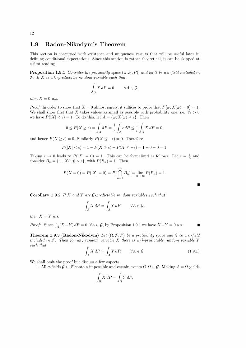
1.9 Radon-Nikodym’s Theorem

This section is concerned with existence and uniqueness results that will be useful later indefining conditional expectations. Since this section is rather theoretical, it can be skipped ata first reading.

Proposition 1.9.1 Consider the probability space (Ω,F , P ), and let G be a σ-field included inF . It X is a G-predictable random variable such that

∫

A

X dP = 0 ∀A ∈ G,

then X = 0 a.s.

Proof: In order to show that X = 0 almost surely, it suffices to prove that P(ω; X(ω) = 0

)= 1.

We shall show first that X takes values as small as possible with probability one, i.e. ∀ε > 0we have P (|X| < ε) = 1. To do this, let A = ω; X(ω) ≥ ε. Then

0 ≤ P (X ≥ ε) =∫

A

dP =1ε

∫

A

ε dP ≤ 1ε

∫

A

X dP = 0,

and hence P (X ≥ ε) = 0. Similarly P (X ≤ −ε) = 0. Therefore

P (|X| < ε) = 1− P (X ≥ ε)− P (X ≤ −ε) = 1− 0− 0 = 1.

Taking ε → 0 leads to P (|X| = 0) = 1. This can be formalized as follows. Let ε = 1n and

consider Bn = ω; |X(ω)| ≤ ε, with P (Bn) = 1. Then

P (X = 0) = P (|X| = 0) = P (∞⋂

n=1

Bn) = limn→∞

P (Bn) = 1.

Corollary 1.9.2 If X and Y are G-predictable random variables such that∫

A

X dP =∫

A

Y dP ∀A ∈ G,

then X = Y a.s.

Proof: Since∫

A(X−Y ) dP = 0, ∀A ∈ G, by Proposition 1.9.1 we have X−Y = 0 a.s.

Theorem 1.9.3 (Radon-Nikodym) Let (Ω,F , P ) be a probability space and G be a σ-fieldincluded in F . Then for any random variable X there is a G-predictable random variable Ysuch that ∫

A

X dP =∫

A

Y dP, ∀A ∈ G. (1.9.1)

We shall omit the proof but discuss a few aspects.1. All σ-fields G ⊂ F contain impossible and certain events Ø, Ω ∈ G. Making A = Ω yields

∫

Ω

X dP =∫

Ω

Y dP,

13

which is E[X] = E[Y ].2. Radon-Nikodym’s theorem states the existence of Y . In fact this is unique almost surely.

In order to show that, assume there are two G-predictable random variables Y1 and Y2 with theaforementioned property. Then from (1.9.1) yields

∫

A

Y1 dP =∫

A

Y2 dP, ∀A ∈ G.

Applying Corollary (1.9.2) yields Y1 = Y2 a.s.

1.10 Conditional Expectation

Let X be a random variable on the probability space (Ω,F , P ). Let G be a σ-field containedin F . Since X is F-predictable, the expectation of X, given the information F must be Xitself. This shall be written as E[X|F ] = X. It is natural to ask what is the expectation of X,given the information G. This is a random variable denoted by E[X|G] satisfying the followingproperties:

1. E[X|G] is G-predictable;

2.∫

AE[X|G] dP =

∫A

X dP, ∀A ∈ G.

E[X|G] is called the conditional expectation of X given G.

We owe a few explanations regarding the correctness of the aforementioned definition. Theexistence of the G-predictable random variable E[X|G] is assured by the Radon-Nikodym the-orem. The almost surely uniqueness is an application of Proposition (1.9.1) (see the discussionpoint 2 of section 1.9).

It worth noting that the expectation of X, denoted by E[X] is a number, while the con-ditional expectation E[X|G] is a random variable. When are they equal and what is theirrelationship? The answers is inferred by the following solved exercises.

Exercise 1.10.1 Show that if G = Ø, Ω, then E[X|G] = E[X].

Proof: We need to show that E[X] satisfies conditions 1 and 2. The first one is obviouslysatisfied since any constant is G-predictable. The latter condition is checked on each set of G.We have

∫

Ω

X dP = E[X] = E[X]∫

Ω

dP =∫

Ω

E[X]dP

∫

Ø

X dP =∫

Ø

E[X]dP.

Exercise 1.10.2 Show that E[E[X|G]] = E[X], i.e. all conditional expectations have the samemean, which is the mean of X.

Proof: Using the definition of expectation and taking A = Ω in the second relation of theaforementioned definition, yields

E[E[X|G]] =∫

Ω

E[X|G] dP =∫

Ω

XdP = E[X],

14

which ends the proof.

Exercise 1.10.3 The conditional expectation of X given the total information F is the randomvariable X itself, i.e.

E[X|F ] = X.

Proof: The random variables X and E[X|F ] are both F-predictable (from the definition ofthe random variable). From the definition of the conditional expectation we have

∫

A

E[X|F ] dP =∫

A

X dP, ∀A ∈ F .

Corollary (1.9.2) implies that E[X|F ] = X almost surely.

General properties of the conditional expectation are stated below without proof. The proofinvolves more or less simple manipulations of integrals and can be taken as an exercise for thereader.

Proposition 1.10.4 Let X and Y be two random variable on the probability space (Ω,F , P ).We have1. Linearity:

E[aX + bY |G] = aE[X|G] + bE[Y |G], ∀a, b ∈ R;

2. Factoring out the predictable part:

E[XY |G] = XE[Y |G]

if X is G-predictable. In particular, E[X|G] = X.3. Tower property:

E[E[X|G]|H] = E[X|H], if H ⊂ G;

4. Positivity:E[X|G] ≥ 0, if X ≥ 0;

5. Expectation of a constant is a constant

E[c|G] = c.

6. An independent condition drops out

E[X|G] = E[X],

if X is independent of G.

1.11 Inequalities of Random Variables

This section prepares the reader for the limits of sequences of random variables and limits ofstochastic processes. We shall start with a classical inequality result regarding expectations:

Theorem 1.11.1 (Jensen’s inequality) Let ϕ : R → R be a convex function and let X bean integrable random variable on the probability space (Ω,F , P ). If ϕ(X) is integrable, then

ϕ(E[X]) ≤ E[ϕ(X)]

almost surely (i.e. the inequality might fail on a set of measure zero).

15

Figure 1.4: Jensen’s inequality ϕ(E[X]) < E[ϕ(X)] for a convex function ϕ.

Proof: Let µ = E[X]. Expand ϕ in a Taylor series about µ and get

ϕ(x) = ϕ(µ) + ϕ′(µ)(x− µ) +12ϕ′′(ξ)(ξ − µ)2,

with ξ in between x and µ. Since ϕ is convex, ϕ′′ ≥ 0, and hence

ϕ(x) ≥ ϕ(µ) + ϕ′(µ)(x− µ),

which means the graph of ϕ(x) is above the tangent line at(x, ϕ(x)

). Replacing x by the

random variable X, and taking the expectation yields

E[ϕ(X)] ≥ E[ϕ(µ) + ϕ′(µ)(X − µ)] = ϕ(µ) + ϕ′(µ)(E[X]− µ)= ϕ(µ) = ϕ(E[X]),

which proves the result.

Fig.1.4 provides a graphical interpretation of Jensen’s inequality. If the distribution of X issymmetric, then the distribution of ϕ(X) is skewed, with ϕ(E[X]) < E[ϕ(X)].

It worth noting that the inequality is reversed for ϕ concave. We shall present next a coupleof applications.

A random variable X : Ω → R is called square integrable if

E[X2] =∫

Ω

|X(ω)|2 dP (ω) =∫

Rx2p(x) dx < ∞.

Application 1.11.2 If X is a square integrable random variable, then it is integrable.

Proof: Jensen’s inequality with ϕ(x) = x2 becomes

E[X]2 ≤ E[X2].

Since the right side is finite, it follows that E[X] < ∞, so X is integrable.

16

Application 1.11.3 If mX(t) denotes the moment generating function of the random variableX with mean µ, then

mX(t) ≥ etµ.

Proof: Applying Jensen inequality with the convex function ϕ(x) = ex yields

eE[X] ≤ E[eX ].

Substituting tX for X yieldseE[tX] ≤ E[etX ]. (1.11.2)

Using the definition of the moment generating function mX(t) = E[etX ] and that E[tX] =tE[X] = tµ, then (1.11.2) leads to the desired inequality.

The variance of a square integrable random variable X is defined by

V ar(X) = E[X2]− E[X]2.

By Application 1.11.2 we have V ar(X) ≥ 0, so there is a constant σX

> 0, called standarddeviation, such that

σ2X

= V ar(X).

Exercise 1.11.4 Prove that a non-constant random variable has a non-zero standard devia-tion.

Exercise 1.11.5 Prove the following identity

V ar[X] = E[(X − E[X])2].

Theorem 1.11.6 (Markov’s inequality) Prove the following inequality

P (ω; |X(ω)| ≥ λ) ≤ 1λp

E[|X|p],

for any p > 0.

Proof: Let A = ω; |X(ω)| ≥ λ. Then

E[|X|p] =∫

Ω

|x|pp(x) dx ≥∫

A

|x|pp(x) dx ≥∫

A

λpp(x) dx

= λp

∫

A

p(x) dx = λpP (A) = λpP (|X| ≥ λ).

Dividing by λp leads to the desired result.

Theorem 1.11.7 (Tchebychev’s inequality) If X is a random variable with mean µ andvariance σ2, show that

P (ω; |X(ω)− µ| ≥ λ) ≤ σ2

λ2.

17

Proof: Let A = ω; |X(ω)− µ| ≥ λ. Then

σ2 = V ar(X) = E[(X − µ)2] =∫

Ω

(x− µ)2p(x) dx ≥∫

A

(x− µ)2p(x) dx

≥ λ2

∫

A

p(x) dx = λ2P (A) = λ2P (ω; |X(ω)− µ| ≥ λ).

Dividing by λ2 leads to the desired inequality.

Theorem 1.11.8 (Chernoff bounds) Let X be a random variable. Then for any λ > 0 wehave

1. P (X ≥ λ) ≤ E[etX ]eλt

, ∀t > 0;

2. P (X ≤ λ) ≤ E[etX ]eλt

, ∀t < 0.

Proof: 1. Let t > 0 and denote Yt = etX . By Markov’s inequality

P (Y ≥ eλt) ≤ E[Y ]eλt

.

Then we have

P (X ≥ λ) = P (tX ≥ λt) = P (etX ≥ eλt)

= P (Y ≥ eλt) ≤ E[Y ]eλt

=E[etX ]

eλt.

2. The case t < 0 is similar.

In the following we shall present an application of the Chernoff bounds for the normaldistributed random variables.

Let X be a random variable normally distributed with mean µ and variance σ2. It is knownthat its moment generating function is given by

m(t) = E[etX ] = eµt+ 12 t2σ2

.

Using the first Chernoff bound we obtain

P (X ≥ λ) ≤ m(t)eλt

= e(µ−λ)t+ 12 t2σ2

, ∀t > 0,

which implies

P (X ≥ λ) ≤ emint>0

[(µ− λ)t +12t2σ2]

.

It is easy to see that the quadratic function f(t) = (µ − λ)t + 12 t2σ2 has the minimum value

reached for t =λ− µ

σ2

mint>0

f(t) = f(λ− µ

σ2

)= − (λ− µ)2

2σ2.

Substituting in the previous formula, we obtain the following result:

18

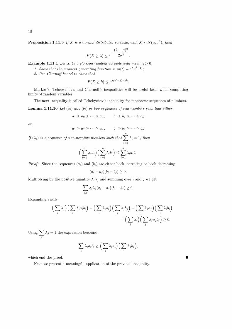
Proposition 1.11.9 If X is a normal distributed variable, with X ∼ N(µ, σ2), then

P (X ≥ λ) ≤ e− (λ− µ)2

2σ2 .

Example 1.11.1 Let X be a Poisson random variable with mean λ > 0.1. Show that the moment generating function is m(t) = eλ(et−1);2. Use Chernoff bound to show that

P (X ≥ k) ≤ eλ(et−1)−tk.

Markov’s, Tchebychev’s and Chernoff’s inequalities will be useful later when computinglimits of random variables.

The next inequality is called Tchebychev’s inequality for monotone sequences of numbers.

Lemma 1.11.10 Let (ai) and (bi) be two sequences of real numbers such that either

a1 ≤ a2 ≤ · · · ≤ an, b1 ≤ b2 ≤ · · · ≤ bn

ora1 ≥ a2 ≥ · · · ≥ an, b1 ≥ b2 ≥ · · · ≥ bn

If (λi) is a sequence of non-negative numbers such thatn∑

i=1

λi = 1, then

( n∑

i=1

λiai

)( n∑

i=1

λibi

)≤

n∑

i=1

λiaibi.

Proof: Since the sequences (ai) and (bi) are either both increasing or both decreasing

(ai − aj)(bi − bj) ≥ 0.

Multiplying by the positive quantity λiλj and summing over i and j we get∑

i,j

λiλj(ai − aj)(bi − bj) ≥ 0.

Expanding yields(∑

j

λj

)(∑

i

λiaibi

)−

( ∑

i

λiai

)( ∑

j

λjbj

)−

( ∑

j

λjaj

)( ∑

i

λibi

)

+( ∑

i

λi

)( ∑

j

λjajbj

)≥ 0.

Using∑

j

λj = 1 the expression becomes

∑

i

λiaibi ≥(∑

i

λiai

)(∑

j

λjbj

),

which end the proof.

Next we present a meaningful application of the previous inequality.

19

Proposition 1.11.11 Let X be a random variable and f and g be two functions, both increas-ing or both decreasing. Then

E[f(X)g(X)] ≥ E[f(X)]E[g(X)]. (1.11.3)

Proof: If X is a discrete random variable, with outcomes x1, · · ·xn, inequality (1.11.3)becomes ∑

j

f(xj)g(xj)p(xj) ≥∑

j

f(xj)p(xj)∑

j

g(xj)p(xj),

where p(xj) = P (X = xj). Denoting aj = f(xj), bj = g(xj), and λj = p(xj), the inequalitytransforms into ∑

j

ajbjλj ≥∑

j

ajλj

∑

j

bjλj ,

which holds true by Lemma 1.11.10.If X is a continuous random variable with the density function p : I → R, the inequality

(1.11.3) can be written in the integral form∫

I

f(x)g(x)p(x) dx ≥∫

I

f(x)p(x) dx

∫

I

g(x)p(x) dx. (1.11.4)

Let x0 < x1 < · · · < xn be a partition of the interval I, with ∆x = xk+1 − xk. Using Lemma1.11.10 we obtain the following inequality between Riemann sums

∑

j

f(xj)g(xj)p(xj)∆x ≥( ∑

j

f(xj)p(xj)∆x)(∑

j

g(xj)p(xj)∆x),

where aj = f(xj), bj = g(xj), and λj = p(xj)∆x. Taking the limit ‖∆x‖ → 0 we obtain(1.11.4), which leads to the desired result.

Exercise 1.11.12 Let f and g be two differentiable functions such that f ′(x)g′(x) > 0, x ∈ I.Then

E[f(X)g(X)] ≥ E[f(X)]E[g(X)],

for any random variable X with values in I.

Exercise 1.11.13 Use Exercise 1.11.12 to show the following inequalities:(a) E[X2] ≥ E[X]2;(b) E[X2 cosh(X)] ≥ E[X2]E[cosh(X)];

(c) E[X sinh(X)] ≥ E[X]E[sinh(X)];(d) E[X6] ≥ E[X2]E[X4];(d) E[X6] ≥ E[X]E[X5];(e) E[X6] ≥ E[X3]2.

Exercise 1.11.14 For any n, k ≥ 1, k ≤ 2n show that

E[X2n] ≥ E[Xk]E[X2n−k].

Can you prove a similar inequality for E[X2n+1]?

20

1.12 Limits of Sequences of Random Variables

Consider a sequence (Xn)n≥1 of random variables defined on the probability space (Ω,F , P ).There are several ways of making sense of the limit expression X = lim

n→∞Xn, and they will be

discussed in the following.

Almost Certain Limit

The sequence Xn converges almost certainly to X, if for all states of the world ω, except a setof probability zero, we have

limn→∞

Xn(ω) = X(ω).

More precisely, this meansP

(ω; lim

n→∞Xn(ω) = X(ω)

)= 1,

and we shall write ac-limn→∞

Xn = X. An important example where this type of limit occurs isthe Strong Law of Large Numbers:

If Xn is a sequence of independent and identically distributed random variables with the

same mean µ, then ac-limn→∞

X1 + · · ·+ Xn

n= µ.

It worth noting that this type of convergence is known also under the name of strongconvergence. This is the reason why the the aforementioned theorem bares its name.

Mean Square Limit

Another possibility of convergence is to look at the mean square deviation of Xn from X. Wesay that Xn converges to X in the mean square if

limn→∞

E[(Xn −X)2] = 0.

More precisely, this should be interpreted as

limn→∞

∫ (Xn(ω)−X(ω)

)2dP (ω) = 0.

This limit will be abbreviated by ms-limn→∞

Xn = X. The mean square convergence is usefulwhen defining the Ito integral.

Example 1.12.1 Consider a sequence Xn of random variables such that there is a constant kwith E[Xn] → k and V ar(Xn) → 0 as n →∞. Show that ms-lim

n→∞Xn = k.

Proof: Since we have

E[|Xn − k|2] = E[X2n − 2kXn + k2] = E[X2

n]− 2kE[Yn] + k2

=(E[X2

n]− E[Xn]2)

+(E[Xn]2 − 2kE[Yn] + k2

)

= V ar(Xn) +(E[Xn]− k

)2,

the right side tends to 0 when taking the limit n →∞.

21

Limit in Probability or Stochastic Limit

The random variable X is the stochastic limit of Xn if for n large enough the probability ofdeviation from X can be made smaller than any arbitrary ε. More precisely, for any ε > 0

limn→∞

P(ω; |Xn(ω)−X(ω)| ≤ ε

)= 1.

This can be written also as

limn→∞

P(ω; |Xn(ω)−X(ω)| > ε

)= 0.

This limit is denoted by st-limn→∞

Xn = X.It worth noting that both almost certain convergence and convergence in mean square

imply the stochastic convergence. Hence, the stochastic convergence is weaker than the afore-mentioned two convergence cases. This is the reason why it is also called the weak convergence.One application is the Weak Law of Large Numbers:

If X1, X2, . . . are identically distributed with expected value µ and if any finite number of

them are independent, then st-limn→∞

X1 + · · ·+ Xn

n= µ.

Proposition 1.12.1 The convergence in the mean square implies the stochastic convergence.

Proof: Let ms-limn→∞

Yn = Y . Let ε > 0 arbitrary fixed. Applying Markov’s inequality withX = Yn − Y , p = 2 and λ = ε, yields

0 ≤ P (|Yn − Y | ≥ ε) ≤ 1ε2

E[|Yn − Y |2].

The right side tends to 0 as n →∞. Applying the Squeeze Theorem we obtain

limn→∞

P (|Yn − Y | ≥ ε) = 0,

which means that Yn converges stochastic to Y .

Exercise 1.12.2 Let Xn be a sequence of random variables such that E[|Xn|] → 0 as n →∞.Prove that st-lim

n→∞Xn = 0.

Proof: Let ε > 0 be arbitrary fixed. We need to show

limn→∞

P(ω; |Xn(ω)| ≥ ε

)= 0. (1.12.5)

From Markov’s inequality (see Exercise 1.11.6) we have

0 ≤ P(ω; |Xn(ω)| ≥ ε

) ≤ E[|Xn|]ε

.

Using Squeeze Theorem we obtain (1.12.5).

Remark 1.12.3 The conclusion still holds true even in the case when there is a p > 0 suchthat E[|Xn|p] → 0 as n →∞.

22

Limit in Distribution

We say the sequence Xn converges in distribution to X if for any continuous bounded functionϕ(x) we have

limn→∞

ϕ(Xn) = ϕ(X).

This type of limit is even weaker than the stochastic convergence, i.e. it is implied by it.An application of the limit in distribution is obtained if consider ϕ(x) = eitx. In this

case, if Xn converges in distribution to X, then the characteristic function of Xn converges tothe characteristic function of X. In particular, the probability density of Xn approachers theprobability density of X.

It can be shown that the convergence in distribution is equivalent with

limn→∞

Fn(x) = F (x),

whenever F is continuous at x, where Fn and F denote the distribution functions of Xn andX, respectively. This is the reason why this convergence bares its name.

1.13 Properties of Limits

Lemma 1.13.1 If ms-limn→∞

Xn = 0 and ms-limn→∞

Yn = 0, then

1. ms-limn→∞

(Xn + Yn) = 0

2. ms-limn→∞

(XnYn) = 0.

Proof: Since ms-limn→∞

Xn = 0, then limn→∞

E[X2n] = 0. Applying the Squeeze Theorem to the

inequality2

0 ≤ E[Xn]2 ≤ E[X2n]

yields limn→∞

E[Xn] = 0. Then

limn→∞

V ar[Xn] = limn→∞

(E[X2

n]− limn→∞

E[Xn]2)

= limn→∞

E[X2n]− lim

n→∞E[Xn]2

= 0.

Similarly, we have limn→∞

E[Y 2n ] = 0, lim

n→∞E[Yn] = 0 and lim

n→∞V ar[Yn] = 0. Then lim

n→∞σXn

=lim

n→∞σ

Yn= 0. Using the correlation formula

Corr(Xn, Yn) =Cov(Xn, Yn)

σXnσYn

,

and the fact that |Corr(Xn, Yn)| ≤ 1, yields

0 ≤ |Cov(Xn, Yn)| ≤ σXn

σYn

.

2This follows from the fact that V ar[Xn] ≥ 0.

23

Since limn→∞

σXn

σXn

= 0, from the Squeeze Theorem it follows that

limn→∞

Cov(Xn, Yn) = 0.

Taking n →∞ in the relation

Cov(Xn, Yn) = E[Xn, Yn]− E[Xn]E[Yn]

yields limn→∞

E[XnYn] = 0. Using the previous relations, we have

limn→∞

E[(Xn + Yn)2] = limn→∞

E[X2n + 2XnYn + Y 2

n ]

= limn→∞

E[X2n] + 2 lim

n→∞E[XnYn] + lim

n→∞E[Y 2

n ]

= 0,

which means ms-limn→∞

(Xn + Yn) = 0.

Proposition 1.13.2 If the sequences of random variables Xn and Yn converge in the meansquare, then

1. ms-limn→∞

(Xn + Yn) = ms-limn→∞

Xn + ms-limn→∞

Yn

2. ms-limn→∞

(cXn) = c ·ms-limn→∞

Xn, ∀c ∈ R.

Proof: 1. Let ms-limn→∞

Xn = L and ms-limn→∞

Yn = M . Consider the sequences X ′n = Xn−L and

Y ′n = Yn −M . Then ms-lim

n→∞X ′

n = 0 and ms-limn→∞

Y ′n = 0. Applying Lemma 1.13.1 yields

ms-limn→∞

(X ′n + Y ′

n) = 0.This is equivalent with

ms-limn→∞

(Xn − L + Yn −M) = 0,which becomes

ms-limn→∞

(Xn + Yn) = L + M .

1.14 Stochastic Processes

A stochastic process on the probability space (Ω,F , P ) is a family of random variables Xt

parameterized by t ∈ T, where T ⊂ R. If T is an interval we say that Xt is a stochastic processin continuous time. If T = 1, 2, 3, . . . we shall say that Xt is a stochastic process in discretetime. The later case describes a sequence of random variables. The aforementioned types ofconvergence can be easily extended to continuous time. For instance, Xt converges in strongsense to X as t →∞ if

P(ω; lim

t→∞Xt(ω) = X(ω)

)= 1.

The evolution in time of a given state of the world ω ∈ Ω given by the function t 7−→ Xt(ω) iscalled a path or realization of Xt. The study of stochastic processes using computer simulationsis based on retrieving information about the process Xt given a large number of it realizations.

24

Consider that all the information accumulated until time t is contained by the σ-field Ft.This means that Ft contains the information of which events have already occurred until thetime t, and which did not. Since the information is growing in time, we have

Fs ⊂ Ft ⊂ F

for any s, t ∈ T with s ≤ t. The family Ft is called a filtration.A stochastic process Xt is called adapted to the filtration Ft if Xt is Ft- predictable, for any

t ∈ T.

Example 1.14.1 Here there are a few examples of filtrations:1. Ft represents the information about the evolution of a stock until time t, with t > 0.2. Ft represents the information about the evolution of a Black-Jack game until time t, with

t > 0.

Example 1.14.2 If X is a random variable, consider the conditional expectation

Xt = E[X|Ft].

From the definition of the conditional expectation, the random variable Xt is Ft-predictable, andcan be regarded as the measurement of X at time t using the information Ft. If the accumulatedknowledge Ft increases and eventually equals the σ-field F , then X = E[X|F ], i.e. we obtainthe entire random variable. The process Xt is adapted to Ft.

Example 1.14.3 Don Joe is asking the doctor how long he still has to live. The age at whichhe will pass away is a random variable, denoted by X. Given his medical condition today, whichis contained in Ft, the doctor infers that Mr. Joe will die at the age of Xt = E[X|Ft]. Thestochastic process Xt is adapted to the medical knowledge Ft.

We shall define next an important type of stochastic process.

Definition 1.14.4 A process Xt, t ∈ T, is called a martingale with respect to the filtration Ft

if1. Xt is integrable for each t ∈ T;2. Xt is adapted to the filtration Ft;3. Xs = E[Xt|Fs], ∀s < t.

Remark 1.14.5 The first condition states that the unconditional forecast is finite E[|Xt]] =∫

Ω

|Xt| dP < ∞. Condition 2 says that the value Xt is known, given the information set Ft.

The third relation asserts that the best forecast of unobserved future values is the last observationon Xt.

Remark 1.14.6 If the third condition is replaced by3′. Xs ≤ E[Xt|Fs], ∀s ≤ t

then Xt is called a submartingale; and if it is replaced by3′′. Xs ≥ E[Xt|Fs], ∀s ≤ t

then Xt is called a supermartingale.It worth noting that Xt is submartingale if and only if −Xt is supermartingale.

25

Example 1.14.1 Let Xt denote Mr. Li Zhu’s salary after t years of work in the same company.Since Xt is known at time t and it is bounded above, as all salaries are, then the first twoconditions hold. Being honest, Mr. Zhu expects today that his future salary will be the same astoday’s, i.e. Xs = E[Xt|Fs], for s < t. This means that Xt is a martingale.

Example 1.14.2 If in the previous example Mr. Zhu is optimistic and believes as today thathis future salary will increase, then Xt is a submartingale.

Example 1.14.3 If X is an integrable random variable on (Ω,F , P ), and Ft is a filtration,then Xt = E[X|Ft] is a martingale.

Example 1.14.4 Let Xt and Yt be martingales with respect to the filtration Ft. Show that forany a, b, c ∈ R the process Zt = aXt + bYt + c is a Ft-martingale.

Example 1.14.5 Let Xt and Yt be martingales with respect to the filtration Ft. Is the processXtYt a martingale with respect to Ft?

In the following, if Xt is a stochastic process, the minimum amount of information resultedfrom knowing the process Xt until time t is denoted by σ(Xs; s ≤ t). In the case of a discreteprocess, we have σ(Xk; k ≤ n).

Example 1.14.6 Let Xn, n ≥ 0 be a sequence of integrable independent random variables.Let S0 = X0, Sn = X0 + · · · + Xn. If E[Xn] ≥ 0, then Sn is a σ(Xk; k ≤ n)-submartingal.In addition, if E[Xn] = 0 and E[X2

n] < ∞, ∀n ≥ 0, then S2n − V ar2(Sn) is a σ(Xk; k ≤ n)-

martingal.

Example 1.14.7 Let Xn, n ≥ 0 be a sequence of independent random variables with E[Xn] = 1for n ≥ 0. Then Pn = X0 ·X1 · · · ·Xn is a σ(Xk; k ≤ n)-martingal.

In chapter 8.1 we shall encounter several processes which are martingales.

Chapter 2

Useful Stochastic Processes

2.1 The Brownian Motion

The observation made first by the botanist Robert Brown in 1827, that small pollen grainssuspended in water have a very irregular and unpredictable state of motion, led to the definitionof the Brownian motion, which is formalized in the following.

Definition 2.1.1 A Brownian motion process is a stochastic process Bt, t ≥ 0, which satisfies1. The process starts at the origin, B0 = 0;2. Bt has stationary, independent increments;3. The process Bt is continuous in t;4. The increments Bt −Bs are normally distributed with mean zero and variance |t− s|,

Bt −Bs ∼ N(0, |t− s|).

The process Xt = x+Bt has all the properties of a Brownian motion that starts at x. SinceBt −Bs is stationary, its distribution function depends only on the time interval t− s, i.e.

P (Bt+s −Bs ≤ a) = P (Bt −B0 ≤ a) = P (Bt ≤ a).

From condition 4 we get that Bt is normally distributed with mean E[Bt] = 0 and V ar[Bt] = t

Bt ∼ N(0, t).

Let 0 < s < t. Since the increments are independent, we can write

E[BsBt] = E[(Bs −B0)(Bt −Bs) + B2s ] = E[Bs −B0]E[Bt −Bs] + E[B2

s ] = s.

Proposition 2.1.2 A Brownian motion process Bt is a martingale with respect to the infor-mation set Ft = σ(Bs; s ≤ t).

Proof: Let s < t and write Bt = Bs + (Bt −Bs). Then

E[Bt|Fs] = E[Bs + (Bt −Bs)|Fs]= E[Bs|Fs] + E[Bt −Bs|Fs]= Bs,

27

28

where we used that Bs is Fs-measurable (from where E[Bs|Fs] = Bs) and that the incrementBt−Bs is independent of previous values of Bt contained in the information set Ft = σ(Bs; s ≤t).

A process with similar properties as the Brownian motion was introduced by Wiener.

Definition 2.1.3 A Wiener process Wt is a process adapted to a filtration Ft such that1. The process starts at the origin, W0 = 0;2. Wt is an Ft-martingale with E[W 2

t ] < ∞ for all t ≥ 0 and

E[(Wt −Ws)2] = t− s, s ≤ t;

3. The process Wt is continuous in t.

Since Wt is a martingale, its increments are unpredictable and hence E[Ws −Wt] = 0; inparticular E[Wt] = 0. It is easy to show that

V ar[Wt −Ws] = |t− s|, V ar[Wt] = t.

The only property Bt has and Wt seems not to have is that the increments are normallydistributed. However, there is no distinction between these two processes, as the followingresult states.

Theorem 2.1.4 (Levy) A Wiener process is a Brownian motion process.

In stochastic calculus we often need to use infinitesimal notations and its properties. If dWt

denotes the infinitesimal increment of a Wiener process in the time interval dt, the aforemen-tioned properties become dWt ∼ N(0, dt), E[dWt] = 0, and E[(dWt)2] = dt.

Proposition 2.1.5 If Wt is a Wiener process with respect to the information set Ft, thenYt = W 2

t − t is a martingale.

Proof: Let s < t. Using that the increments Wt −Ws and (Wt −Ws)2 are independent of theinformation set Fs and applying Proposition 1.10.4 yields

E[W 2t |Fs] = E[(Ws + Wt −Ws)2|Fs]

= E[W 2s + 2Ws(Wt −Ws) + (Wt −Ws)2|Fs]

= E[W 2s |Fs] + E[2Ws(Wt −Ws)|Fs] + E[(Wt −Ws)2|Fs]

= W 2s + 2WsE[Wt −Ws|Fs] + E[(Wt −Ws)2|Fs]

= W 2s + 2WsE[Wt −Ws] + E[(Wt −Ws)2]

= W 2s + t− s,

and hence E[W 2t − t|Fs] = W 2

s − s, for s < t.

The following result states the memoryless property of Brownian motion1

Proposition 2.1.6 The conditional distribution of Wt+s, given the present Wt and the pastWu, 0 ≤ u < t, depends only on the present.

1These type of processes are called Marcov processes

29

Proof: Using the independent increment assumption, we have

P (Wt+s ≤ c|Wt = x,Wu, 0 ≤ u < t)= P (Wt+s −Wt ≤ c− x|Wt = x,Wu, 0 ≤ u < t)= P (Wt+s −Wt ≤ c− x)= P (Wt+s ≤ c|Wt = x).

Since Wt is normally distributed with mean 0 and variance t, its density function is

φt(x) =1√2πt

e−x22t .

Then its distribution function is

Ft(x) = P (Wt ≤ x) =1√2πt

∫ x

−∞e−

u22t du

The probability that Wt is between the values a and b is given by

P (a ≤ Wt ≤ b) =1√2πt

∫ b

a

e−u22t du, a < b.

Even if the increments of a Brownian motion are independent, its values are still correlated.

Proposition 2.1.7 Let 0 ≤ s ≤ t. Then1. Cov(Ws,Wt) = s;

2. Corr(Ws,Wt) =√

s

t.

Proof: 1. Using the properties of covariance

Cov(Ws,Wt) = Cov(Ws,Ws + Wt −Ws)= Cov(Ws,Ws) + Cov(Ws,Wt −Ws)= V ar(Ws) + E[Ws(Wt −Ws)]− E[Ws]E[Wt −Ws]= s + E[Ws]E[Wt −Ws]= s,

since E[Ws] = 0.

We can arrive to the same result starting from the formula

Cov(Ws,Wt) = E[WsWt]− E[Ws]E[Wt] = E[WsWt].

Using the tower property and that Wt is a martingale, we have

E[WsWt] = E[E[WsWt|Fs]] = E[WsE[Wt|Fs]]= E[WsWs] = E[W 2

s ] = s,

so Cov(Ws,Wt) = s.

30

2. The correlation formula yields

Corr(Ws,Wt) =Cov(Ws, Wt)σ(Wt)σ(Ws)

=s√s√

t=

√s

t.

Remark 2.1.8 Removing the order relation between s and t, the previous relations can be alsostated as

Cov(Ws,Wt) = mins, t;

Corr(Ws,Wt) =

√mins, tmaxs, t .

The following exercises state the translation and the scaling invariance of the Brownianmotion.

Exercise 2.1.9 For any t0 ≥ 0, show that the process Xt = Wt+t0−Wt0 is a Brownian motion.

Exercise 2.1.10 For any λ > 0, show that the process Xt = 1√λWλt is a Brownian motion.

Exercise 2.1.11 Let 0 < s < t < u. Show the following multiplicative property

Corr(Ws,Wt)Corr(Wt,Wu) = Corr(Ws,Wu).

Research topic: Find all stochastic processes with the aforementioned property.

Exercise 2.1.12 (a) Use the martingale property of W 2t − t to find

E[(W 2t − t)(W 2

s − s)];

(b) Evaluate E[W 2t W 2

s ];(c) Compute Cov(W 2

t ,W 2s );

(d) Find Corr(W 2t , W 2

s ).

Exercise 2.1.13 Consider the process Yt = tW 1t, t > 0.

(a) Find the distribution of Yt;(b) Find Cov(Ys, Yt);(c) Is Yt a Brownian motion process?

Exercise 2.1.14 The process Xt = |Wt| is called Brownian motion reflected at the origin.Show that(a) E[|Wt|] =

√2t/π;

(b) V ar(|Wt|) = (1− 2π )t.

Research topic: Find all functions g(t) and h(t) such that the process Xt = g(t)Wh(t) is aBrownian motion.

Exercise 2.1.15 Let 0 < s < t. Find E[W 2t |Fs].

Exercise 2.1.16 Let 0 < s < t. Show that(a) E[W 3

t |Fs] = 3(t− s)Ws + W 3s ;

(b) E[W 4t |Fs] = 3(t− s)2 + 6(t− s)W 2

s + W 4s .

31

50 100 150 200 250 300 350

-1.0

-0.5

50 100 150 200 250 300 350

2

3

4

5

a b

Figure 2.1: a Three simulations of the Brownian motion process Wt; b Two simulations of thegeometric Brownian motion process eWt .

2.2 Geometric Brownian Motion

The process Xt = eWt , t ≥ 0 is called geometric Brownian motion. A few simulations of thisprocess are depicted in Fig.2.1 b. The following result will be useful in the sequel.

Lemma 2.2.1 We have E[eαWt ] = eα2t/2, for α ≥ 0.

Proof: Using the definition of the expectation

E[eαWt ] =∫

eαxφt(x) dx =1√2πt

∫e−

x22t +sx dx

= eα2t/2,

where we have used the integral formula∫

e−ax2+bx dx =π

ae

b24a , a > 0

with a = 12t and b = s.

Proposition 2.2.2 The geometric Brownian motion Xt = eWt is log-normally distributed withmean et/2 and variance e2t − et.

Proof: Since Wt is normally distributed, then Xt = eWt will have a log-normal distribution.Using Lemma 2.2.1 we have

E[Xt] = E[eWt ] = et/2

E[X2t ] = E[e2Wt ] = e2t,

and hence the variance is

V ar[Xt] = E[X2t ]− E[Xt]2 = e2t − (et/2)2 = e2t − et.

32

The distribution function can be obtained by reducing to the distribution function of aBrownian motion

FXt(x) = P (Xt ≤ x) = P (eWt ≤ x)

= P (Wt ≤ ln x) = FWt

(ln x)

=1√2πt

∫ ln x

−∞e−

u22t du.

The density function of the geometric Brownian motion Xt = eWt is given by

p(x) =d

dxFXt

(x) =

1x√

2πte−(ln x)2/(2t), if x > 0,

0, elsewhere.

Exercise 2.2.3 If Xt = eWt , find the covariance Cov(Xs, Xt).

Exercise 2.2.4 Let Xt = eWt .(a) Show that Xt is not a martingale.(b) Show that e−

t2 Xt is a martingale.

2.3 Integrated Brownian Motion

The stochastic process

Zt =∫ t

0

Ws ds, t ≥ 0

is called integrated Brownian motion.Let 0 = s0 < s1 < · · · < sk < · · · sn = t, with sk = kt

n . Then Zt can be written as a limit ofRiemann sums

Zt = limn→∞

n∑

k=1

Wsk∆s = t lim

n→∞Ws1 + · · ·+ Wsn

n.

We are tempted to apply the Central Limit Theorem, but Wskare not independent, so we need

to transform the sum into a sum of independent normally distributed random variables first.A straightforward computation shows that

Ws1 + · · ·+ Wsn

= n(Ws1 −W0) + (n− 1)(Ws2 −Ws1) + · · ·+ (Wsn −Wsn−1)= X1 + X2 + · · ·+ Xn. (2.3.1)

Since the increments of a Brownian motion are independent and normally distributed, we have

X1 ∼ N(0, n2∆s

)

X2 ∼ N(0, (n− 1)2∆s

)

X3 ∼ N(0, (n− 2)2∆s

)

· · · · · · · · · · · · · · · · · · · · · · · ·Xn ∼ N

(0, ∆s

).

Recall now the following variant of the Central Limit Theorem:

33

Theorem 2.3.1 If Xj are independent random variables normally distributed with mean µj

and variance σ2j , then the sum X1+· · ·+Xn is also normally distributed with mean µ1+· · ·+µn

and variance σ21 + · · ·+ σ2

n.

Then

X1 + · · ·+ Xn ∼ N(0, (1 + 22 + 32 + · · ·+ n2)∆s

)= N

(0,

n(n + 1)(2n + 1)6

∆s),

with ∆s =t

n. Using (2.3.1) yields

tWs1 + · · ·+ Wsn

n∼ N

(0,

(n + 1)(2n + 1)6n2

t3).

Taking the limit we get

Zt ∼ N(0,

t3

3

).

Proposition 2.3.2 The integrated Brownian motion Zt has a Gaussian distribution with mean0 and variance t3/3.

The mean and the variance can be also computed in a direct way as follows. By Fubini’stheorem we have

E[Zt] = E[∫ t

0

Ws ds] =∫

R

∫ t

0

Ws ds dP

=∫ t

0

∫

RWs dP ds =

∫ t

0

E[Ws] ds = 0,

since E[Ws] = 0. Then the variance is given by

V ar[Zt] = E[Z2t ]− E[Zt]2 = E[Z2

t ]

= E[∫ t

0

Wu du ·∫ t

0

Wv dv] = E[∫ t

0

∫ t

0

WuWv dudv]

=∫ t

0

∫ t

0

E[WuWv] dudv =∫∫

[0,t]×[0,t]

minu, v dudv

=∫∫

D1

minu, v dudv +∫∫

D2

minu, v dudv, (2.3.2)

whereD1 = (u, v); u < v, 0 ≤ u ≤ t, D2 = (u, v); u > v, 0 ≤ u ≤ t

The first integral can be evaluated using Fubini’s theorem∫∫

D1

minu, v dudv =∫∫

D1

v dudv

=∫ t

0

( ∫ u

0

v dv)

du =∫ t

0

u2

2du =

t3

6.

Similarly, the latter integral is equal to∫∫

D2

minu, v dudv =t3

6.

34

Substituting in (2.3.2) yields

V ar[Zt] =t3

6+

t3

6=

t3

3.

Exercise 2.3.3 (a) Prove that the moment generating function of Zt is

m(u) = eu2t3/6.

(b) Use the first part to find the mean and variance of Zt.

Exercise 2.3.4 Let s < t. Show that the covariance of the integrated Brownian motion is givenby

Cov[Zs, Zt] = s2( t

2− s

6

).

Exercise 2.3.5 Show that(a) Cov[Zt, Zt − Zt−h] = 1

2 t2h + o(h).

(b) Cov[Zt,Wt] =t2

2.

Exercise 2.3.6 Consider the process Xt =∫ t

0

eWs ds.

(a) Find the mean of Xt;(b) Find the variance of Xt;(c) What is the distribution of Xt?

2.4 Exponential Integrated Brownian Motion

If Zt =∫ t

0Ws ds denotes the integrated Brownian motion, the process

Vt = eZt

is called exponential integrated Brownian motion. The process starts at V0 = e0 = 1. Since Zt

is normally distributed, then Vt is log-normally distributed. We shall compute the mean andthe variance in a direct way. Using Exercise 2.3.3 we have

E[Vt] = E[eZt ] = m(1) = et36

E[V 2t ] = E[e2Zt ] = m(2) = e

4t36 = e

2t33

V ar[Vt] = E[V 2t ]− E[Vt]2 = e

2t33 − e

t33 .

2.5 Brownian Bridge

The process Xt = Wt− tW1 is called the Brownian bridge tied down at both 0 and 1. Since wecan also write

Xt = Wt − tWt − tW1 + tWt

= (1− t)(Wt −W0)− t(W1 −Wt),

35

using that the increments Wt −W0 and W1 −Wt are independent and normally distributed,with

Wt −W0 ∼ N(0, t), W1 −Wt ∼ N(0, 1− t),

it follows that Xt is normally distributed with

E[Xt] = (1− t)E[(Wt −W0)]− tE[(W1 −Wt)] = 0V ar[Xt] = (1− t)2V ar[(Wt −W0)] + t2V ar[(W1 −Wt)]

= (1− t)2(t− 0) + t2(1− t)= t(1− t).

This can be also stated by saying that the Brownian bridge tied at 0 and 1 is a Gaussian processwith mean 0 and variance t(1− t).

2.6 Brownian Motion with Drift

The process Yt = µt + Wt, t ≥ 0, is called Brownian motion with drift. The process Xt tendsto drift off at a rate µ. It starts at Y0 = 0 and it is a Gaussian process with mean

E[Yt] = µt + E[Wt] = µt

and varianceV ar[Yt] = V ar[µt + Wt] = V ar[Wt] = t.

2.7 Bessel Process

This section deals with the process satisfied by the Euclidean distance from the origin to aparticle following a Brownian motion in Rn. More precisely, if W1(t), · · · ,Wn(t) are independentBrownian motions, let W (t) = (W1(t), · · · ,Wn(t)) be a Brownian motion in Rn, n ≥ 2. Theprocess

Rt = dist(O,W (t)) =√

W1(t)2 + · · ·+ Wn(t)2

is called n-dimensional Bessel process.

The probability density of this process is given by the following result.

Proposition 2.7.1 The probability density function of Rt, t > 0 is given by

pt(ρ) =

2(2t)n/2 Γ(n/2)

ρn−1e−ρ2

2t , ρ ≥ 0;

0, ρ < 0

with

Γ(n

2

)=

(n2 − 1)! for n even;

(n2 − 1)(n

2 − 2) · · · 32

12

√π, for n odd.

36

Proof: Since the Brownian motions W1(t), . . . , Wn(t) are independent, their joint densityfunction is

fW1···Wn

(t) = fW1

(t) · · · fWn

(t)

=1

(2πt)n/2e−(x2

1+···+x2n)/(2t), t > 0.

In the next computation we shall use the following formula of integration that follows fromthe use of polar coordinates

∫

|x|≤ρf(x) dx = σ(Sn−1)

∫ ρ

0

rn−1g(r) dr, (2.7.3)

where f(x) = g(|x|) is a function on Rn with spherical symmetry, and where

σ(Sn−1) =2πn/2

Γ(n/2)

is the area of the (n− 1)-dimensional sphere in Rn.

Let ρ ≥ 0. The distribution function of Rt is

FR(ρ) = P (Rt ≤ ρ) =

∫

Rt≤ρf

W1···Wn(t) dx1 · · · dxn

=∫

x21+···+x2

n≤ρ2

1(2πt)n/2

e−(x21+···+x2

n)/(2t) dx1 · · · dxn

=∫ ρ

0

rn−1

(∫

S(0,1)

1(2πt)n/2

e−(x21+···+x2

n)/(2t) dσ

)dr

=σ(Sn−1)(2πt)n/2

∫ ρ

0

rn−1 e−r2/(2t) dr.

Differentiating yields

pt(ρ) =d

dρF

R(ρ) =

σ(Sn−1)(2πt)n/2

ρn−1e−ρ2

2t

=2

(2t)n/2Γ(n/2)ρn−1e−

ρ2

2t , ρ > 0, t > 0.

It worth noting that in the 2-dimensional case the aforementioned density becomes a partic-ular case of a Weibull distribution with parameters m = 2 and α = 2t, called Wald’s distribution

pt(x) =1txe−

x22t , x > 0, t > 0.

37

2.8 The Poisson Process

A Poisson process describes the number of occurrences of a certain event before time t, suchas: the number of electrons arriving at an anode until time t; the number of cars arriving at agas station until time t; the number of phone calls received in a certain day until time t; thenumber of visitors entering a museum in a certain day until time t; the number of earthquakesoccurred in Japan during time interval [0, t]; the number of shocks in the stock market fromthe beginning of the year until time t; the number of twisters that might hit Alabama duringa decade.

2.8.1 Definition and Properties

The definition of a Poisson process is stated more precisely in the following.

Definition 2.8.1 A Poisson process is a stochastic process Nt, t ≥ 0, which satisfies1. The process starts at the origin, N0 = 0;2. Nt has stationary, independent increments;3. The process Nt is right continuous in t, with left hand limits;4. The increments Nt − Ns, with 0 < s < t, have a Poisson distribution with parameter

λ(t− s), i.e.

P (Nt −Ns = k) =λk(t− s)k

k!e−λ(t−s).

It can be shown that condition 4 in the previous definition can be replaced by the followingtwo conditions:

P (Nt −Ns = 1) = λ(t− s) + o(t− s) (2.8.4)P (Nt −Ns ≥ 2) = o(t− s), (2.8.5)

where o(h) denotes a quantity such that limh→0 o(h)/h = 0. This means the probability that ajump of size 1 occurs in the infinitesimal interval dt is equal to λdt, and the probability that atleast 2 events occur in the same small interval is zero. This implies that the random variabledNt may take only two values, 0 and 1, and hence satisfies

P (dNt = 1) = λ dt (2.8.6)P (dNt = 0) = 1− λ dt. (2.8.7)

The fact that Nt −Ns is stationary can be stated as

P (Nt+s −Ns ≤ n) = P (Nt −N0 ≤ n) = P (Nt ≤ n) =n∑

k=0

(λt)k

k!e−λt.

From condition 4 we get the mean and variance of increments

E[Nt −Ns] = λ(t− s), V ar[Nt −Ns] = λ(t− s).

In particular, the random variable Nt is Poisson distributed with E[Nt] = λt and V ar[Nt] = λt.The parameter λ is called the rate of the process. This means that the events occur at theconstant rate λ.

38

Since the increments are independent, we have

E[NsNt] = E[(Ns −N0)(Nt −Ns) + N2s ]

= E[Ns −N0]E[Nt −Ns] + E[N2s ]

= λs · λ(t− s) + (V ar[Ns] + E[Ns]2)= λ2st + λs. (2.8.8)

As a consequence we have the following result:

Proposition 2.8.2 Let 0 ≤ s ≤ t. Then1. Cov(Ns, Nt) = λs;

2. Corr(Ns, Nt) =√

s

t.

Proof: 1. Using (2.8.8) we have

Cov(Ns, Nt) = E[NsNt]− E[Ns]E[Nt]= λ2st + λs− λsλt

= λs.

2. Using the formula for the correlation yields

Corr(Ns, Nt) =Cov(Ns, Nt)

(V ar[Ns]V ar[Nt])1/2=

λs

(λsλt)1/2=

√s

t.

It worth noting the similarity with Proposition 2.1.7.

Proposition 2.8.3 Let Nt be Ft-adapted. Then the process Mt = Nt − λt is a martingale.

Proof: Let s < t and write Nt = Ns + (Nt −Ns). Then

E[Nt|Fs] = E[Ns + (Nt −Ns)|Fs]= E[Ns|Fs] + E[Nt −Ns|Fs]= Ns + E[Nt −Ns]= Ns + λ(t− s),

where we used that Ns is Fs-measurable (and hence E[Ns|Fs] = Ns) and that the incrementNt − Ns is independent of previous values of Ns and the information set Fs. Subtracting λtyields

E[Nt − λt|Fs] = Ns − λs,

or E[Mt|Fs] = Ms. Since it is obvious that Mt is Ft-adapted, it follows that Mt is a martingale.

It worth noting that the Poisson process Nt is not a martingale. The martingale processMt = Nt − λt is called the compensated Poisson process.

Exercise 2.8.4 Compute E[N2t |Fs]. Is the process N2

t a martingale?

39

Exercise 2.8.5 (i) Show that the moment generating function of the random variable Nt is

mNt

(x) = eλt(ex−1).

(ii) Find the expressions E[N2t ], E[N3

t ], and E[N4t ].

Exercise 2.8.6 Find the mean and variance of the process Xt = eNt .

Exercise 2.8.7 (i) Show that the moment generating function of the random variable Mt is

mMt

(x) = eλt(ex−x−1).

(ii) Let s < t. Verify that

E[Mt −Ms] = 0,

E[(Mt −Ms)2] = λ(t− s),E[(Mt −Ms)3] = λ(t− s),E[(Mt −Ms)4] = λ(t− s) + 3λ2(t− s)2.

Exercise 2.8.8 Let s < t. Show that

V ar[Nt −Ns] = λ(t− s),V ar[(Mt −Ms)2] = λ(t− s) + 2λ2(t− s)2.

2.8.2 Interarrival times

For each state of the world ω, the path t → Nt(ω) is a step function that exhibits unit jumps.Each jump in the path corresponds to an occurrence of a new event. Let T1 be the randomvariable which describes the time of the 1st jump. Let T2 be the time between the 1st jumpand the second one. In general, denote by Tn the time elapsed between the (n− 1)th and nthjumps. The random variables Tn are called interarrival times.

Proposition 2.8.9 The random variables Tn are independent and exponentially distributedwith mean E[Tn] = 1/λ.

Proof: We start by noticing that the events T1 > t and Nt = 0 are the same, since bothdescribe the situation that no events occurred until time t. Then

P (T1 > t) = P (Nt = 0) = P (Nt −N0 = 0) = e−λt,

and hence the distribution function of T1 is

FT1(t) = P (T1 ≤ t) = 1− P (T1 > t) = 1− e−λt.

Differentiating yields the density function

fT1

(t) =d

dtFT1(t) = λe−λt.

40

It follows that T1 is has an exponential distribution, with E[T1] = 1/λ. The conditionaldistribution of T2 is

F (t|s) = P (T2 ≤ t|T1 = s) = 1− P (T2 > t|T1 = s)

= 1− P (T2 > t, T1 = s)P (T1 = s)

= 1− P(0 jumps in (s, s + t], 1 jump in (0, s]

)

P (T1 = s)

= 1− P(0 jumps in (s, s + t]

)P

(1 jump in (0, s]

)

P(1 jump in (0, s]

)

= 1− P (Ns+t −Ns = 0) = 1− e−λt,

which is independent of s. Then T2 is independent of T1 and exponentially distributed. Asimilar argument for any Tn leads to the desired result.

2.8.3 Waiting times

The random variable Sn = T1 + T2 + · · · + Tn is called the waiting time until the nth jump.The event Sn ≤ t means that there are n jumps that occurred before or at time t, i.e. thereare at least n events that happened up to time t; the event is equal to Nt ≥ n. Hence thedistribution function of Sn is given by

FSn(t) = P (Sn ≤ t) = P (Nt ≥ n) = e−λt∞∑

k=n

(λt)k

k!.

Differentiating we obtain the density function of the waiting time Sn

fSn(t) =d

dtFSn(t) =

λe−λt(λt)n−1

(n− 1)!.

Writing

fSn(t) =tn−1e−λt

(1/λ)nΓ(n),

it turns out that Sn has a gamma distribution with parameters α = n and β = 1/λ. It followsthat

E[Sn] =n

λ, V ar[Sn] =

n

λ2.

The relation limn→∞

E[Sn] = ∞ states that the expectation of the waiting time gets unboundedlarge as n →∞.

2.8.4 The Integrated Poisson Process

The function u → Nu is a continuous with the exception of a set of countable jumps of size 1.It is known that such functions are Riemann integrable, so it makes sense to define the process

Ut =∫ t

0

Nu du,

41

Figure 2.2: The Poisson process Nt and the waiting times S1, S2, · · ·Sn. The shaded rectanglehas area n(Sn+1 − t).

called the integrated Poisson process. The next result provides a relation between the processUt and the partial sum of the waiting times Sk.

Proposition 2.8.10 The integrated Poisson process can be expressed as

Ut = tNt −Nt∑

k=1

Sk.

Let Nt = n. Since Nt is equal to k between the waiting times Sk and Sk+1, the process Ut,which is equal to the area of the subgraph of Nu between 0 and t, can be expressed as

Ut =∫ t

0

Nu du = 1 · (S2 − S1) + 2 · (S3 − S2) + · · ·+ n(Sn+1 − Sn)− n(Sn+1 − t).

Since Sn < t < Sn+1, the difference of the last two terms represents the area of last therectangle, which has the length t − Sn and the height n. Using associativity, a computationyields

1 · (S2 − S1) + 2 · (S3 − S2) + · · ·+ n(Sn+1 − Sn) = nSn+1 − (S1 + S2 + · · ·+ Sn).

Substituting in the aforementioned relation yields

Ut = nSn+1 − (S1 + S2 + · · ·+ Sn)− n(Sn+1 − t)= nt− (S1 + S2 + · · ·+ Sn)

= tNt −Nt∑

k=1

Sk,

where we replaced n by Nt.

42

Exercise 2.8.11 Find the following means(a) E[Ut].

(b) E[ Nt∑

k=1

Sk

].

The following result deals with the quadratic variation of the compensated Poisson processMt = Nt − λt.

Proposition 2.8.12 Let a < b and consider the partition a = t0 < t1 < · · · < tn−1 < tn < b.Then

ms– lim‖∆n‖→∞

n−1∑

k=0

(Mtk+1 −Mtk)2 = Nb −Na, (2.8.9)

where ‖∆n‖ = sup0≤k≤n−1

(tk+1 − tk).

Proof: For the sake of simplicity we shall use the following notations

∆tk = tk+1 − tk, ∆Mk = Mtk+1 −Mtk, ∆Nk = Ntk+1 −Ntk

.

The relation we need to prove can be also written as

ms-limn→∞

n−1∑

k=0

[(∆Mk)2 −∆Nk

]= 0.

LetYk = (∆Mk)2 −∆Nk = (∆Mk)2 + ∆Mk + λ∆tk.

It suffices to show that

E[ n−1∑

k=0

Yk

]= 0, (2.8.10)

limn→∞

V ar[ n−1∑

k=0

Yk

]= 0. (2.8.11)

The first identity follows from the properties of Poisson processes, see Exercise 2.8.7

E[ n−1∑

k=0

Yk

]=

n−1∑

k=0

E[Yk] =n−1∑

k=0

E[(∆Mk)2]− E[∆Nk]

=n−1∑

k=0

(λ∆tk − λ∆tk) = 0.

For the proof of the identity (2.8.11) we need to find first the variance of Yk.

V ar[Yk] = V ar[(∆Mk)2 − (∆Mk + λ∆tk)] = V ar[(∆Mk)2 −∆Mk]= V ar[(∆Mk)2] + V ar[∆Mk]− 2Cov[∆M2

k , ∆Mk]= λ∆tk + 2λ2∆t2k + λ∆tk

−2[E[(∆Mk)3]− E[(∆Mk)2]E[∆Mk]

]

= 2λ2(∆tk)2,

43

where we used Exercise 2.8.7 and the fact that E[∆Mk] = 0. Since Mt is a process withindependent increments, then Cov[Yk, Yj ] = 0 for i 6= j. Then

V ar[ n−1∑

k=0

Yk

]=

n−1∑

k=0

V ar[Yk] + 2∑

k 6=j

Cov[Yk, Yj ] =n−1∑

k=0

V ar[Yk]

= 2λ2n−1∑

k=0

(∆tk)2 ≤ 2λ2‖∆n‖n−1∑

k=0

∆tk = 2λ2(b− a)‖∆n‖,

and hence V ar[ n−1∑

k=0

Yn

]→ 0 as ‖∆n‖ → 0. By Proposition 3.3.1 we obtain the desired limit in

mean square sense.

The previous result states that the quadratic variation of the martingale Mt between a andb is equal to the jump of the Poisson process between a and b.

2.8.5 The Fundamental Relation dM2t = dNt

Recall relation (2.8.9)

ms- limn→∞

n−1∑

k=0

(Mtk+1 −Mtk)2 = Nb −Na. (2.8.12)

The right side can be regarded as a Riemann-Stieltjes integral

Nb −Na =∫ b

a

dNt,

while the left side can be regarded as a stochastic integral with respect to (dMt)2

∫ b

a

(dMt)2 := ms- limn→∞

n−1∑

k=0

(Mtk+1 −Mtk)2.

Substituting in (2.8.12) yields ∫ b

a

(dMt)2 =∫ b

a

dNt,

for any a < b. The equivalent differential form is

dM2t = dNt. (2.8.13)

This relation will be useful in formal calculations involving Ito’s formula.

2.8.6 The Relations dt dMt = 0, dWt dMt = 0

In order to show that dt dMt = 0 in the mean square sense, it suffices to prove the limit

ms- limn→∞

n−1∑

k=0

(tk+1 − tk)(Mtk+1 −Mtk) = 0, (2.8.14)

44

since this is thought as a vanishing integral of the increment process dMt with respect to dt

∫ b

a

dMt dt = 0, ∀a, b ∈ R.

Denote

Xn =n−1∑

k=0

(tk+1 − tk)(Mtk+1 −Mtk) =

n−1∑

k=0

∆tk∆Mk.

In order to show (2.8.16) it suffices to prove that

1. E[Xn] = 0;

2. limn→∞

V ar[Xn] = 0.

using the additivity of the expectation and Exercise 2.8.7, (ii)

E[Xn] = E[ n−1∑

k=0

∆tk∆Mk

]=

n−1∑

k=0

∆tkE[∆Mk] = 0.

Since the Poisson process Nt has independent increments, the same property holds for thecompensated Poisson process Mt. Then ∆tk∆Mk and ∆tj∆Mj are independent for k 6= j, andusing the properties of variance we have

V ar[Xn] = V ar[ n−1∑

k=0

∆tk∆Mk

]=

n−1∑

k=0

(∆tk)2V ar[∆Mk] = λ

n−1∑

k=0

(∆tk)3,

where we usedV ar[∆Mk] = E[(∆Mk)2]− (E[∆Mk])2 = λ∆tk,

see Exercise 2.8.7, (ii). If let ‖∆n‖ = maxk

∆tk, then

V ar[Xn] = λ

n−1∑

k=0

(∆tk)3 ≤ λ‖∆n‖2n−1∑

k=0

∆tk = λ(b− a)‖∆n‖2 → 0

as n →∞. Hence we proved the stochastic differential relation

dt dMt = 0. (2.8.15)

For showing the relation dWt dMt = 0, we need to prove

ms- limn→∞

Yn = 0, (2.8.16)

where we have denoted

Yn =n−1∑

k=0

(Wk+1 −Wk)(Mtk+1 −Mtk) =

n−1∑

k=0

∆Wk∆Mk.

45

Since the Brownian motion Wt and the process Mt have independent increments and ∆Wk isindependent of ∆Mk, we have

E[Yn] =n−1∑

k=0

E[∆Wk∆Mk] =n−1∑

k=0

E[∆Wk]E[∆Mk] = 0,

where we used E[∆Wk] = E[∆Mk] = 0. Using also E[(∆Wk)2] = ∆tk, E[(∆Mk)2] = λ∆tk,invoking the independence of ∆Wk and ∆Mk, we get

V ar[∆Wk∆Mk] = E[(∆Wk)2(∆Mk)2]− (E[∆Wk∆Mk])2

= E[(∆Wk)2]E[(∆Mk)2]− E[∆Wk]2E[∆Mk]2

= λ(∆tk)2.

Then using the independence of the terms in the sum, we get

V ar[Yn] =n−1∑

k=0

V ar[∆Wk∆Mk] = λ

n−1∑

k=0

(∆tk)2

≤ λ‖∆n‖n−1∑

k=0

∆tk = λ(b− a)‖∆n‖ → 0,

as n → ∞. Since Yn is a random variable with mean zero and variance decreasing to zero, itfollows that Yn → 0 in the mean square sense. Hence we proved that

dWt dMt = 0. (2.8.17)

Exercise 2.8.13 Show the following stochastic differential relations(a) dt dNt = 0(b) dWt dNt = 0(c) dt dWt = 0.

The relations proved in this section will be useful in the sequel, when developing the stochas-tic model of a stock price that exhibits jumps modeled by a Poisson process.

Chapter 3

Properties of StochasticProcesses

3.1 Hitting Times

Hitting times are useful in finance when studying barrier options and lookback options. Forinstance, knock-in options enter into existence when the stock price hits a certain barrier beforeoption maturity. A lookback option is priced using the maximum value of the stock until thepresent time. The stock price is not a Brownian motion, but it depends on one. Hence theneed of studying the hitting time for the Brownian motion.

The first result deals with the hitting time for a Brownian motion to reach the barrier a ∈ R,see Fig.3.1.

Lemma 3.1.1 Let Ta be the first time the Brownian motion Wt hits a. Then

P (Ta ≤ t) =2√2π

∫ ∞

|a|/√t

e−y2/2 dy.

a

Ta

Wt

50 100 150 200 250 300 350

1.5

2.0

2.5

Figure 3.1: The first hitting time Ta given by WTa = a.

47

48

Proof: If A and B are two events, then

P (A) = P (A ∩B) + P (A ∩B)= P (A|B)P (B) + P (A|B)P (B). (3.1.1)

Let a > 0. Using formula (3.1.1) for A = ω; Wt(ω) ≥ a and B = ω; Ta(ω) ≤ t yields

P (Wt ≥ a) = P (Wt ≥ a|Ta ≤ t)P (Ta ≤ t)+P (Wt ≥ a|Ta > t)P (Ta > t) (3.1.2)

If Ta > t, the Brownian motion did not reached the barrier a yet, so we must have Wt < a.Therefore

P (Wt ≥ a|Ta > t) = 0.

If Ta ≤ t, then WTa= a. Since the Brownian motion is a Markov process, it starts fresh at Ta.

Due to symmetry of the density function of a normal variable, Wt has equally chances to go upor go down after the time interval t− Ta. It follows that

P (Wt ≥ a|Ta ≤ t) =12.


P (Ta ≤ t) = 2P (Wt ≥ a)

=2√2πt

∫ ∞

a

e−x2/(2t) dx =2√2π

∫ ∞

a/√

t

e−y2/2 dy.

If a < 0, symmetry reasons imply that the distribution of Ta is the same as that of T−a, so weget

P (Ta ≤ t) = P (T−a ≤ t) =2√2π

∫ ∞

−a/√

t

e−y2/2 dy.

Theorem 3.1.2 Let a ∈ R be fixed. Then the Brownian motion hits a in finite time withprobability 1.

Proof: The probability that Wt hits a in finite time is

P (Ta < ∞) = limt→∞

P (Ta ≤ t) = limt→∞

2√2π

∫ ∞

|a|/√t

e−y2/2 dy

=2√2π

∫ ∞

0

e−y2/2 dy = 1,

where we used the well known integral∫ ∞

0

e−y2/2 dy =12

∫ ∞

−∞e−y2/2 dy =

12

√2π.

49

Remark 3.1.3 Even if the hitting time is finite with probability 1, its expectation E[Ta] isinfinite. This means that the expected time to hit the barrier is infinite.

Corollary 3.1.4 A Brownian motion process returns to the origin in finite time with probability1.

Proof: Choose a = 0 and apply Theorem 3.1.2.

Exercise 3.1.5 Show that the distribution function of the process Xt = maxs∈[0,t]

Ws is given by

P (Xt ≤ a) =2√2π

∫ a/√

t

−∞e−y2/2 dy.

The fact that a Brownian motion returns or hits a barrier almost surely is a property char-acteristic to the dimension 1 only. The next result states that in larger dimensions this is nomore possible.

Theorem 3.1.6 Let (a, b) ∈ R2. The 2-dimensional Brownian motion W (t) =(W1(t),W2(t)

)hits the point (a, b) with probability zero. The same result is valid for any n-dimensional Brow-nian motion, with n ≥ 2.

Research topic. This deals with the hitting time of a 2-dimensional Brownian motion to reacha given disk. Let Dε(x0) = x ∈ R2; |x− x0| ≤ ε. Find the probability P (∃t; W (t) ∈ Dε(x0))as a function of x0 and ε. Let TDε(x0) = inft≥0t; W (t) ∈ Dε(x0). Find the distributionand the expectation of the random variable TDε(x0). It is known that P (TDε(x0) < ∞) = 1.However, in the n-dimensional version this probability is zero.

Research topic. This deals with the exit time of a 2-dimensional Brownian motion from thedisc of radius a. Let

Ta = inft>0t; W (t) /∈ D(0, a) = inf

t>0t; |W (t)| > a,

Find the distribution function of the exit time Ta and its expectation. It is known that P (Ta <

∞) = R2

2 . You may try to apply the same argument as in the proof of Lemma 3.1.1; however,because of convexity

P (Rt ≥ a|Ta ≤ t) >12.

What is the exact value of this probability?

Theorem 3.1.7 (The law of Arc-sine) The probability that a Brownian motion Wt does nothave any zeros in the interval (t1, t2) is equal to

P (Wt 6= 0, t1 ≤ t ≤ t2) =2π

arcsin√

t1t2

.

Proof: Let A(a; t1, t2) denote the event that the Brownian motion Wt takes on the value abetween t1 and t2. In particular, A(0; t1, t2) denotes the event that Wt has (at least) a zerobetween t1 and t2. Substituting A = A(0; t1, t2) and X = Wt1 in the following formula ofconditional probability

P (A) =∫

P (A|X = x) PX

(x) =∫

P (A|X = x)fX

(x) dx

50

t t1 2

Wt

a50 100 150 200 250 300 350

-0.6

-0.4

-0.2

0.2

0.4

Figure 3.2: The event A(a; t1, t2) in the Law of Arc-sine.

yields

P(A(0; t1, t2)

)=

∫P

(A(0; t1, t2)|Wt1 = x

)f

Wt1(x) dx (3.1.3)

=1√2πt1

∫ ∞

−∞P

(A(0; t1, t2)|Wt1 = x

)e−

x22t1 dx

Using the properties of Wt with respect to time translation and symmetry we have

P(A(0; t1, t2)|Wt1 = x

)= P

(A(0; 0, t2 − t1)|W0 = x

)

= P(A(−x; 0, t2 − t1)|W0 = 0

)

= P(A(|x|; 0, t2 − t1)|W0 = 0

)

= P(A(|x|; 0, t2 − t1)

)

= P(T|x| ≤ t2 − t1

),

the last identity stating that Wt hits |x| before t2 − t1. Using Lemma 3.1.1 yields

P(A(0; t1, t2)|Wt1 = x

)=

2√2π(t2 − t1)

∫ ∞

|x|e− y2

2(t2−t1) dy.

Substituting in (3.1.3) we obtain

P(A(0; t1, t2)

)=

1√2πt1

∫ ∞

−∞

( 2√2π(t2 − t1)

∫ ∞

|x|e− y2

2(t2−t1) dy)e−

x22t1 dx

=1

π√

t1(t2 − t1)

∫ ∞

0

∫ ∞

|x|e− y2

2(t2−t1)− x22t1 dydx.

The above integral can be evaluated to get (see Exercise 3.1.8 )

P(A(0; t1, t2)

)= 1− 2

πarcsin

√t1t2

.

Using P (Wt 6= 0, t1 ≤ t ≤ t2) = 1− P(A(0; t1, t2)

)we obtain the desired result.

51

Exercise 3.1.8 Use polar coordinates to show

1π√

t1(t2 − t1)

∫ ∞

0

∫ ∞

|x|e− y2

2(t2−t1)− x22t1 dydx = 1− 2

πarcsin

√t1t2

.

Exercise 3.1.9 Find the probability that a 2-dimensional Brownian motion W (t) =(W1(t),W2(t)

)stays in the same quadrant for the time interval t ∈ (t1, t2).

Exercise 3.1.10 Find the probability that a Brownian motion Wt does not take the value a inthe interval (t1, t2).

Exercise 3.1.11 Let a 6= b. Find the probability that a Brownian motion Wt does not take anyof the values a, b in the interval (t1, t2). Formulate and prove a generalization.

Research topic. What is the probability that a 2-dimensional Brownian process hits a set Dbetween time instances t1 and t2?

We provide below a similar result without proof.

Theorem 3.1.12 (Arc-sine Law of Levy) Let L+t =

∫ t

0sgn+Ws ds be the amount of time a

Brownian motion Wt is positive during the time interval [0, t]. Then

P (L+t ≤ τ) =

2π

arcsin√

τ

t.

Research topic. Let Lt(D) be the amount of time spent by a 2-dimensional Brownian motionW (t) inside the set D. Find P (Lt(D) ≤ τ). When D is the half-plane (x, y); y > 0 we retrievethe previous result.

Theorem 3.1.13 Let Xt = µt + Wt denote a Brownian motion with nonzero drift rate µ, andconsider α, β > 0. Then

P (Xt goes up to α before down to − β) =e2µβ − 1

e2µβ − e−2µα.

3.2 Limits of Stochastic Processes

Let (Xt)t≥0 be a stochastic process. One can make sense of the limit expression X = limt→∞

Xt,in a similar way as we did in section 1.12 for sequences of random variables. We shall re-writethe definitions for the continuous case.

Almost Certain Limit

The process Xt converges almost certainly to X, if for all states of the world ω, except a set ofprobability zero, we have

limt→∞

Xt(ω) = X(ω).

We shall write ac-limt→∞

Xt = X. It is also called sometimes strong convergence.

52

Mean Square Limit

We say that the process Xt converges to X in the mean square if

limt→∞

E[(Xt −X)2] = 0.

In this case we write ms-limt→∞

Xt = X.

Limit in Probability or Stochastic Limit

The stochastic process Xt converges in stochastic limit to X if

limt→∞

P(ω; |Xt(ω)−X(ω)| > ε

)= 0.

This limit is abbreviated by st-limt→∞

Xt = X.It worth noting that, like in the case of sequences of random variables, both almost certain

convergence and convergence in mean square imply the stochastic convergence.

Limit in Distribution

We say that Xt converges in distribution to X if for any continuous bounded function ϕ(x) wehave

limt→∞

ϕ(Xt) = ϕ(X).

It worth noting that the stochastic convergence implies the convergence in distribution.

3.3 Convergence Theorems

The following property is a reformulation of the Exercise 1.12.1 in the continuous setup.

Proposition 3.3.1 Consider a stochastic process Xt such that E[Xt] → k, constant, andV ar(Xt) → 0 as t →∞. Then ms-lim

t→∞Xt = k.

Next we shall provide a few applications that show how some processes compare with powersof t for t large.

Application 3.3.2 If α > 1/2, then

ms-limt→∞

Wt

tα= 0.

Proof: Let Xt =Wt

tα. Then E[Xt] =

E[Wt]tα

= 0, and V ar[Xt] =1

t2αV ar[Wt] =

t

t2α=

1t2α−1

,

for any t > 0. Since1

t2α−1→ 0 as t → ∞, applying Proposition 3.3.1 yields ms-lim

t→∞Wt

tα= 0.

Corollary 3.3.3 We have ms-limt→∞

Wt

t= 0.

53

Application 3.3.4 Let Zt =∫ t

0Ws ds. If β > 3/2, then

ms-limt→∞

Zt

tβ= 0.

Proof: Let Xt =Zt

tβ. Then E[Xt] =

E[Zt]tβ

= 0, and V ar[Xt] =1

t2βV ar[Zt] =

t3

3t2β=

13t2β−3

,

for any t > 0. Since1

3t2β−3→ 0 as t → ∞, applying Proposition 3.3.1 leads to the desired

result.

Application 3.3.5 For any p > 0, c ≥ 1 we have

ms-limt→∞

eWt−ct

tp= 0.

Proof: Consider the process Xt =eWt−ct

tp=

eWt

tpect. Since

E[Xt] =E[eWt ]tpect

=et/2

tpect=

1e(c− 1

2 )t

1tp→ 0, as t →∞

V ar[Xt] =V ar[eWt ]t2pe2ct

=e2t − et

t2pe2ct=

1t2p

( 1e2t(c−1)

− 1et(2c−1)

)→ 0.

Proposition 3.3.1 leads to the desired result.

Application 3.3.6 If β > 1/2, then

ms-limt→∞

max0≤s≤t

Ws

tβ= 0.

Proof: Let Xt =max0≤s≤t

Ws

tβ. There is an s ∈ [0, t] such that Ws = max

0≤s≤tWs, so Xt =

Ws

tβ. The

mean and the variance satisfy

E[Xt] =E[Ws]

tβ= 0

V ar[Xt] =V ar[Ws]

t2β=

s

t2β≤ t

t2β=

1t2β−1

→ 0, t →∞.

Apply Proposition 3.3.1 and get the desired result.

Remark 3.3.7 The strongest result regarding limits of Brownian motion is called the law ofiterated logarithms and was first proved by Lamperti:

limt→∞

supWt√

2t ln ln t= 1,

almost certainly.

Proposition 3.3.8 Let Xt be a stochastic process. Then

ms-limt→∞

Xt = 0 ⇐⇒ ms-limt→∞

X2t = 0.

54

Proof: Left as an exercise.

Exercise 3.3.9 Let Xt be a stochastic process. Show that

ms-limt→∞

Xt = 0 ⇐⇒ ms-limt→∞

|Xt| = 0.

Another convergence result can be obtained if consider the continuous analog of Exercise1.12.2:

Proposition 3.3.10 Let Xt be a stochastic process such that there is a p > 0 such thatE[|Xt|p] → 0 as t →∞. Then st-lim

t→∞Xt = 0.

Application 3.3.11 We shall show that for any α > 1/2

st-limt→∞

Wt

tα= 0.

Proof: Consider the process Xt =Wt

tα. By Proposition 3.3.8 it suffices to show st-lim

t→∞X2

t = 0.Since

E[|Xt|2] = E[X2t ] = E

[W 2t

t2α

]=

E[W 2t ]

t2α=

t

t2α=

1t2α−1

→ 0, t →∞,

then Proposition 3.3.10 yields st-limt→∞

X2t = 0.

The following result can be regarded as the L’Hospital’s rule for sequences:

Lemma 3.3.12 (Cesaro-Stoltz) Let xn and yn be two sequences of real numbers, n ≥ 1. If

the limit limn→∞

xn+1 − xn

yn+1 − ynexists and it is equal to L, then the following limit exists

limn→∞

xn

yn= L.

Proof: (Sketch) Assume there are differentiable functions f and g such that f(n) = xn andg(n) = yn. (How do you construct these functions?) From Cauchy’s theorem1 there is acn ∈ (n, n + 1) such that

L = limn→∞

xn+1 − xn

yn+1 − yn= lim

n→∞f(n + 1)− f(n)g(n + 1)− g(n)

= limn→∞

f ′(cn)g′(cn)

.

Since cn →∞ as n →∞, we can write the aforementioned limit also as

limt→∞

f ′(t)g′(t)

= L.

(Here one may argue against this, but we recall the freedom of choice for the functions f andg such that cn can be any number between n and n + 1). By l’Hospital’s rule we get

limt→∞

f(t)g(t)

= L.

1This says that if f and g are differentiable on (a, b) and continuous on [a, b], then there is a c ∈ (a, b) such

thatf(a)− f(b)

g(a)− g(b)=

f ′(c)g′(c)

.

55

Making t = n yields limt→∞

xn

yn= L.

The next application states that if a sequence is convergent, then the arithmetic average ofits terms is also convergent, and the sequences have the same limit.

Example 3.3.1 Let an be a convergent sequence with limn→∞

an = L. Let

An =a1 + a2 + · · ·+ an

n

be the arithmetic average of the first n terms. Show that An is convergent and

limn→∞

An = L.

Proof: This is an application of Cesaro-Stoltz lemma. Consider the sequences xn = a1 + a2 +· · ·+ an and yn = n. Since

xn+1 − xn

yn+1 − yn=

(a1 + · · ·+ an+1)− (a1 + · · ·+ an)(n + 1)− n

=an+1

1,

thenlim

n→∞xn+1 − xn

yn+1 − yn= lim

n→∞an+1 = L.

Applying the Cesaro-Stoltz lemma yields

limn→∞

An = limn→∞

xn

yn= L.

Exercise 3.3.13 Let bn be a convergent sequence with limn→∞

bn = L. Let

Gn = (b1 · b2 · · · · · bn)1/n

be the geometric average of the first n terms. Show that Gn is convergent and

limn→∞

Gn = L.

The following result extends the Cesaro-Stoltz lemma to sequences of random variables.

Proposition 3.3.14 Let Xn be a sequence of random variables on the probability space (Ω,F , P ),such that

ac-limn→∞

Xn+1 −Xn

Yn+1 − Yn= L.

Then

ac-limn→∞

Xn

Yn= L.

Proposition 3.3.15 Consider the sets

A = ω ∈ Ω; limn→∞

Xn+1(ω)−Xn(ω)Yn+1(ω)− Yn(ω)

= L

B = ω ∈ Ω; limn→∞

Xn(ω)Yn(ω)

= L.

56

Since for any given state of the world ω, the sequences xn = Xn(ω) and yn = Yn(ω) arenumerical sequences, Lemma 3.3.12 yields the inclusion A ⊂ B. This implies P (A) ≤ P (B).Since P (A) = 1, it follows that P (B) = 1, which leads to the desired conclusion.

Remark 3.3.16 Let Xn and Yn denote the prices of two stocks in the day n. The previousresult states that if Corr(Xn+1−Xn, Yn+1−Yn) → 1, as n →∞, then Corr(Xn, Yn) → 1. So,if the correlation of the the daily changes of the stock price tends to 1 in the long run, then thestock prices correlation does the same.

Example 3.3.17 Let Sn denote the price of a stock in the day n, and assume thatac-lim

n→∞Sn = L.

Then

ac-limn→∞

S1 + · · ·+ Sn

n= L and ac-lim

n→∞(S1 · · · · · Sn)1/n = L.

This says, that if almost all future simulations of the stock price approach the steady statelimit L, the arithmetic and geometric averages converge to the same limit. The statement is aconsequence of Proposition 3.3.14 and follows a similar proof as Example 3.3.1. Asian optionshave payoffs depending on these type of averages, as we shall se in the sequel.

Research topic: Extend Proposition 3.3.14 to the continuous case of stochastic processes.

3.3.1 The Martingale Convergence Theorem

We state now a result which is a powerful way of proving almost certain convergence.

Theorem 3.3.18 Let Xn be a martingale with bounded means

∃M > 0 such that E[|Xn|] ≤ M, ∀n ≥ 1. (3.3.4)

Then there is L < ∞ such that

P(ω; lim

n→∞Xn(ω) = L

)= 1.

Since E[|Xn|]2 ≤ E[X2n], the boundness condition (3.3.4) can be replaced by its stronger version

∃M > 0 such that E[X2n] ≤ M, ∀n ≥ 1.

Example 3.3.2 It is known that Xt = eWt−t/2 is a martingale. Since

E[Xt] = E[eWt−t/2] = e−t/2E[eWt ] = e−t/2et/2 = 1,

by the Martingale Convergence Theorem there is a number L such that Xt → L a.c. as t →∞.What is the limit L? How did you make your guess?

3.3.2 The Squeeze Theorem

The following result is the analog of the Squeeze Theorem from usual Calculus.

Theorem 3.3.19 Let Xn, Yn, Zn be sequences of random variables on the probability space(Ω,F , P ) such that

Xn ≤ Yn ≤ Zn a.s. ∀n ≥ 1.

If Xn and Zn converge to L as n → ∞ almost certainly (or in mean square, or stochastic orin distribution), then Yn converges to L in a similar mode.

57

Proof: For any state of the world ω ∈ Ω consider the sequences xn = Xn(ω), yn = Yn(ω) andzn = Zn(ω) and apply the usual Squeeze Theorem to them.

Remark 3.3.20 The previous theorem remains valid if n is replaced by a continuous positiveparameter t.

Example 3.3.3 Show that ac-limt→∞

Wt sin(Wt)t

= 0.

Proof: Consider the sequences Xt = 0, Yt =Wt sin(Wt)

tand Zt =

Wt

t. From Application

3.3.11 we have ac-limt→∞

Zt = 0. Applying the Squeeze Theorem we obtain the desired result.

Chapter 4

Stochastic Integration

This chapter deals with one of the most useful stochastic integral, called the Ito integral. Thistype of stochastic integral was introduced in 1944 by the Japanese mathematician K. Ito, andwas originally motivated by a construction of diffusion processes.

4.0.3 Nonanticipating Processes

Consider the Brownian motion Wt. A process Ft is called nonanticipating process if Ft isindependent of the increment Wt′ −Wt for any t and t′ with t < t′. Consequently, the processFt is independent of the behavior of the Brownian motion in the future, i.e. it cannot anticipatethe future. For instance, Wt, eWt , W 2

t −Wt +t are examples of nonanticipating processes, whileWt+1 or 1

2 (Wt+1 −Wt)2 are not.Nonanticipating processes are important because the Ito integral concept applies only to

them.If Ft denotes the information known until time t, where this information is generated by

the Brownian motion Ws; s ≤ t, then any Ft-adapted process Ft is nonanticipating.

4.0.4 Increments of Brownian Motions

In this section we shall discuss a few basic properties of the increments of a Brownian motion,which will be useful when computing stochastic integrals.

Proposition 4.0.21 Let Wt be a Brownian motion. If s < t, we have1. E[(Wt −Ws)2] = t− s.2. V ar[(Wt −Ws)2] = 2(t− s)2.

Proof: 1. Using that Wt −Ws ∼ N(0, t− s), we have

E[(Wt −Ws)2] = E[(Wt −Ws)2]− (E[Wt −Ws])2 = V ar(Wt −Ws) = t− s.

2. Dividing by the standard deviation yields the standard normal random variableWt −Ws√

t− s∼

N(0, 1). Its square,(Wt −Ws)2

t− sis χ2-distributed with 1 degree of freedom.1 Its mean is 1 and

1A χ2-distributed random variable with n degrees of freedom has mean n and variance 2n.

59

60

its variance is 2. This implies

E[ (Wt −Ws)2

t− s

]= 1 =⇒ E[(Wt −Ws)2] = t− s;

V ar[ (Wt −Ws)2

t− s

]= 2 =⇒ V ar[(Wt −Ws)2] = 2(t− s)2.

Remark 4.0.22 The infinitesimal version of the previous result is obtained by replacing t− swith dt

1. E[dW 2t ] = dt;

2. V ar[dW 2t ] = 2dt2.

We shall see in a next section that in fact dW 2t and dt are equal in a mean square sense.

Exercise 4.0.23 Show that

1. E[(Wt −Ws)4] = 3(t− s)2;

2. E[(Wt −Ws)6] = 15(t− s)3.

4.1 The Ito Integral

The Ito integral is defined in a way that is similar to the Riemann integral. The Ito integralis taken with respect to infinitesimal increments of a Brownian motion dWt, which are randomvariables, while the Riemann integral considers integration with respect to the predictableinfinitesimal changes dt. It worth noting that the Ito integral is a random variable, while theRiemann integral is just a real number. Despite this fact, there are several common propertiesand relations between these two types of integral.

Consider 0 ≤ a < b and let Ft = f(Wt, t) be a nonanticipating process with

E[ ∫ b

a

F 2t dt

]< ∞.

Divide the interval [a, b] into n subintervals using the partition points

a = t0 < t1 < · · · < tn−1 < tn = b,

and consider the partial sums

Sn =n−1∑

i=0

Fti(Wti+1 −Wti).

We emphasize that the intermediate points are the left endpoints of each interval, and this isthe way they should be always chosen. Since the process Ft is nonanticipative, the randomvariables Fti and Wti+1 −Wti are independent; this is an important feature in the definition ofthe Ito integral.

The Ito integral is the limit of the partial sum Sn

61

ms-limn→∞

Sn =∫ T

0

Ft dWt,

provided the limit exists. It can be shown that the choice of partition does not influence thevalue of the Ito integral. This is the reason why, for practical purposes, it suffices to assumethe intervals equidistant, i.e.

ti+1 − ti = a +(b− a)

n, i = 0, 1, · · · , n− 1.

The previous convergence is in the mean square sense, i.e.

limn→∞

E[(

Sn −∫ b

a

Ft dWt

)2]= 0.

Existence of Ito integral

It is known that the Ito stochastic integral∫ b

a

Ft dWt exists if the process Ft = f(Wt, t) satisfies

the following two properties:1. The paths ω → Ft(ω) are continuous on [a, b] for any state of the world ω ∈ Ω;2. The process Ft is nonanticipating for t ∈ [a, b].

For instance, the following stochastic integrals exist:

∫ T

0

W 2t dWt,

∫ T

0

sin(Wt) dWt,

∫ b

a

cos(Wt)t

dWt.

4.2 Examples of Ito integrals

As in the case of Riemann integral, using the definition is not an efficient way of computingintegrals. The same philosophy applies to Ito integrals. We shall compute in the following twosimple Ito integrals. In later sections we shall introduce more efficient methods for computingIto integrals.

4.2.1 The case Ft = c, constant

In this case the partial sums can be computed explicitly

Sn =n−1∑

i=0

Fti(Wti+1 −Wti) =n−1∑

i=0

c(Wti+1 −Wti)

= c(Wb −Wa),

and since the answer does not depend on n, we have∫ b

a

c dWt = c(Wb −Wa).

In particular, taking c = 1, since the Brownian motion starts at 0, we have the following formula

∫ T

0

dWt = WT .

62

4.2.2 The case Ft = Wt

We shall integrate the process Wt between 0 and T . Considering an equidistant partition, we

take tk =kT

n, k = 0, 1, · · · , n− 1. The partial sums are given by

Sn =n−1∑

i=0

Wti(Wti+1 −Wti).

Sincexy =

12[(x + y)2 − x2 − y2],

letting x = Wti and y = Wti+1 −Wti yields

Wti(Wti+1 −Wti

) =12W 2

ti+1− 1

2W 2

ti− 1

2(Wti+1 −Wti

)2.

Then after pair cancelations the sum becomes

Sn =12

n−1∑

i=0

W 2ti+1

− 12

n−1∑

i=0

W 2ti− 1

2

n−1∑

i=0

(Wti+1 −Wti)2

=12W 2

tn− 1

2

n−1∑

i=0

(Wti+1 −Wti)2

Using tn = T , we get

Sn =12W 2

T −12

n−1∑

i=0

(Wti+1 −Wti)2.

Since the first term is independent of n, we have

ms- limn→∞

Sn =12W 2

T −ms- limn→∞

12

n−1∑

i=0

(Wti+1 −Wti)2. (4.2.1)

In the following we shall compute the right term limit. Denote

Xn =n−1∑

i=0

(Wti+1 −Wti)2.

Since the increments are independent, Proposition 4.0.21 yields

E[Xn] =n−1∑

i=0

E[(Wti+1 −Wti)2] =

n−1∑

i=0

(ti+1 − ti)

= tn − t0 = T ;

V ar[Xn] =n−1∑

i=0

V ar[(Wti+1 −Wti)2] =

n−1∑

i=0

2(ti+1 − ti)2

=2T

n2,

63

where we used that the partition is equidistant. Since Xn satisfies the conditions

E[Xn] = T, ∀n ≥ 1;V ar[Xn] → 0, n →∞,

by Proposition 3.3.1 we obtain ms-limn→∞

Xn = T , or

ms- limn→∞

n−1∑

i=0

(Wti+1 −Wti)2 = T. (4.2.2)

This states that the quadratic variation of the Brownian motion is T . Hence (4.2.1) becomes

ms- limn→∞

Sn =12W 2

T −12T.

We have obtained the following explicit formula of a stochastic integral

∫ T

0

Wt dWt =12W 2

T −12T.

In a similar way one can obtain

∫ b

a

Wt dWt =12(W 2

b −W 2a )− 1

2(b− a).

It worth noting that the right side contains random variables depending on the limits of inte-gration a and b.

Exercise 4.2.1 Show the following identities

1. E[∫ T

0dWt] = 0;

2. E[∫ T

0WtdWt] = 0;

3. V ar[∫ T

0WtdWt] = T 2.

4.3 The Fundamental Relation dW 2t = dt

The relation discussed in this section can be regarded as the fundamental relation of StochasticCalculus. We shall start by recalling relation (4.2.2)

ms- limn→∞

n−1∑

i=0

(Wti+1 −Wti)2 = T. (4.3.3)

The right side can be regarded as a regular Riemann integral

T =∫ T

0

dt,

64

while the left side can be regarded as a stochastic integral with respect to dW 2t

∫ T

0

(dWt)2 := ms- limn→∞

n−1∑

i=0

(Wti+1 −Wti)2.


∫ T

0

(dWt)2 =∫ T

0

dt, ∀T > 0.

The differential form of this integral equation is

dW 2t = dt.

Roughly speaking, the process dW 2t , which is the square of infinitesimal increments of a Brow-

nian motion, is totally predictable. This relation is plays a central role in Stochastic Calculusand it will be useful when dealing with Ito’s Lemma.

4.4 Properties of the Ito Integral

We shall start with some properties which are similar with those of the Riemannian integral.

Proposition 4.4.1 Let f(Wt, t), g(Wt, t) be nonanticipating processes and c ∈ R. Then wehave

1. Additivity:

∫ T

0

[f(Wt, t) + g(Wt, t)] dWt =∫ T

0

f(Wt, t) dWt +∫ T

0

g(Wt, t) dWt.

2. Homogeneity: ∫ T

0

cf(Wt, t) dWt = c

∫ T

0

f(Wt, t) dWt.

3. Partition property:

∫ T

0

f(Wt, t) dWt =∫ u

0

f(Wt, t) dWt +∫ T

u

f(Wt, t) dWt, ∀0 < u < T.

Proof: 1. Consider the partial sum sequences

Xn =n−1∑

i=0

f(Wti , ti)(Wti+1 −Wti)

Yn =n−1∑

i=0

g(Wti , ti)(Wti+1 −Wti).

65

Since ms-limn→∞

Xn =∫ T

0

f(Wt, t) dWt and ms-limn→∞

Yn =∫ T

0

g(Wt, t) dWt, using Proposition

1.13.2 yields∫ T

0

(f(Wt, t) + g(Wt, t)

)dWt

= ms-limn→∞

n−1∑

i=0

(f(Wti , ti) + g(Wti , ti)

)(Wti+1 −Wti)

= ms-limn→∞

[ n−1∑

i=0

(f(Wti

, ti)(Wti+1 −Wti) +

n−1∑

i=0

g(Wti, ti)(Wti+1 −Wti

)]

= ms-limn→∞

(Xn + Yn) = ms-limn→∞

Xn + ms-limn→∞

Yn

=∫ T

0

f(Wt, t) dWt +∫ T

0

g(Wt, t) dWt.

The proof of the parts 2 and 3 are left as an exercise to the reader.

Some other properties, such as monotonicity, do not hold in general. It is possible to have anonnegative random variable Ft for which the random variable

∫ T

0Ft dWt has negative values.

Some of the random variable properties of the Ito integral are given by the following result.

Proposition 4.4.2 We have1. Zero mean:

E[ ∫ b

a

f(Wt, t) dWt

]= 0.

2. Isometry:

E[( ∫ b

a

f(Wt, t) dWt

)2]= E

[ ∫ b

a

f(Wt, t)2 dt].

3. Covariance:

E[( ∫ b

a

f(Wt, t) dWt

)(∫ b

a

g(Wt, t) dWt

)]= E

[ ∫ b

a

f(Wt, t)g(Wt, t) dt].

We shall discuss the previous properties giving rough reasons why they hold true. Thedetailed proofs are beyond the goal of this books.

1. The Ito integral is the mean square limit of the partial sums Sn =∑n−1

i=0 fti(Wti+1 −Wti), where we denoted fti = f(Wti , ti). Since f(Wt, t) is nonanticipative process, then fti isindependent of the increments Wti+1 −Wti , and then we have

E[Sn] = E[ n−1∑

i=0

fti(Wti+1 −Wti)]

=n−1∑

i=0

E[fti(Wti+1 −Wti)]

=n−1∑

i=0

E[fti ]E[(Wti+1 −Wti)] = 0,

because the increments have mean zero. Since each partial sum has zero mean, their limit,which is the Ito Integral, will also have zero mean.

66

2. Since the square of the sum of partial sums can be written as

S2n =

( n−1∑

i=0

fti(Wti+1 −Wti

))2

=n−1∑

i=0

f2ti

(Wti+1 −Wti)2 + 2

∑

i 6=j

fti(Wti+1 −Wti)ftj (Wtj+1 −Wtj ),

using the independence yields

E[S2n] =

n−1∑

i=0

E[f2ti

]E[(Wti+1 −Wti)2]

+2∑

i 6=j

E[fti]E[(Wti+1 −Wti

)]E[ftj]E[(Wtj+1 −Wtj

)]

=n−1∑

i=0

E[f2ti

](ti+1 − ti),

which are the Riemann sums of the integral∫ b

a

E[f2t ] dt = E

[ ∫ b

a

ft dt], where the last identity

follows from Fubini’s theorem. Hence E[S2n] converges to the aforementioned integral. It is yet

to be shown that the convergence holds also in mean square.

3. Consider the partial sums

Sn =n−1∑

i=0

fti(Wti+1 −Wti), Vn =n−1∑

j=0

gtj (Wtj+1 −Wtj ).

Their product is

SnVn =( n−1∑

i=0

fti(Wti+1 −Wti))( n−1∑

j=0

gtj (Wtj+1 −Wtj ))

=n−1∑

i=0

ftigti(Wti+1 −Wti)2 +

n−1∑

i 6=j

ftigtj (Wti+1 −Wti)(Wtj+1 −Wtj )

Using that ft and gt are nonanticipative and that

E[(Wti+1 −Wti)(Wtj+1 −Wtj )] = E[Wti+1 −Wti ]E[Wtj+1 −Wtj ] = 0, i 6= j

E[(Wti+1 −Wti)2] = ti+1 − ti,

it follows that

E[SnVn] =n−1∑

i=0

E[ftigti ]E[(Wti+1 −Wti)2]

=n−1∑

i=0

E[ftigti ](ti+1 − ti),

67

which is the Riemann sum for the integral∫ b

aE[ftgt] dt.

From 1 and 2 it follows that the random variable∫ b

af(Wt, t) dWt has mean zero and variance

V ar[ ∫ b

a

f(Wt, t) dWt

]= E

[ ∫ b

a

f(Wt, t)2 dt].

From 1 and 3 it follows that

Cov[ ∫ b

a

f(Wt, t) dWt,

∫ b

a

g(Wt, t) dWt

]=

∫ b

a

E[f(Wt, t)g(Wt, t)] dt.

Corollary 4.4.3 (Cauchy’s integral inequality) Let f(t) = f(Wt, t) and g(t) = g(Wt, t).Then ( ∫ b

a

E[ftgt] dt)2

≤( ∫ b

a

E[f2t ] dt

)( ∫ b

a

E[g2t ] dt

).

Proof: It follows from the previous theorem and from the correlation formula |Corr(X,Y )| =|Corr(X, Y )|

[V ar(X)V ar(Y )]1/2≤ 1.

Let Ft be the information set at time t. This implies that fti and Wti+1 −Wti are known

at time t, for any ti+1 ≤ t. It follows that the partial sum Sn =n−1∑

i=0

fti(Wti+1 − Wti) is

Ft-predictable. The following result states that this is also valid in mean square:

Proposition 4.4.4 The Ito integral∫ t

0fs dWs is Ft-predictable.

The following two results state that if the upper limit of an Ito integral is replaced by theparameter t we obtain a continuous martingale.

Proposition 4.4.5 For any s < t we have

E[ ∫ t

0

f(Wu, u) dWu|Fs

]=

∫ s

0

f(Wu, u) dWu.

Proof: Using part 3 of Proposition 4.4.2 we get

E[ ∫ t

0

f(Wu, u) dWu|Fs

]

= E[ ∫ s

0

f(Wu, u) dWu +∫ t

s

f(Wu, u) dWu|Fs

]

= E[ ∫ s

0

f(Wu, u) dWu|Fs

]+ E

[ ∫ t

s

f(Wu, u) dWu|Fs

]. (4.4.4)

Since∫ s

0f(Wu, u) dWu is Fs-predictable (see Proposition 4.4.4), by part 2 of Proposition 1.10.4

E[ ∫ s

0

f(Wu, u) dWu|Fs

]=

∫ s

0

f(Wu, u) dWu.

68

Since∫ t

sf(Wu, u) dWu contains only information between s and t, it is unpredictable given the

information set Fs, so

E[ ∫ t

s

f(Wu, u) dWu|Fs

]= 0.

Substituting in (4.4.4) yields the desired result.

Proposition 4.4.6 Consider the process Xt =∫ t

0f(Ws, s) dWs. Then Xt is continuous, i.e.

for almost any state of the world ω ∈ Ω, the path t → Xt(ω) is continuous.

Proof: A rigorous proof is beyond the purpose of this book. We shall provide a rough sketch.Assume the process f(Wt, t) satisfies E[f(Wt, t)2] < M , for some M > 0. Let t0 be fixed andconsider h > 0. Consider the increment Yh = Xt0+h−Xt0 . Using the aforementioned propertiesof the Ito integral we have

E[Yh] = E[Xt0+h −Xt0 ] = E[ ∫ t0+h

t0

f(Wt, t) dWt

]= 0

E[Y 2h ] = E

[( ∫ t0+h

t0

f(Wt, t) dWt

)2]=

∫ t0+h

t0

E[f(Wt, t)2] dt

< M

∫ t0+h

t0

dt = Mh.

The process Yh has zero mean for any h > 0 and its variance tends to 0 as h → 0. Using aconvergence theorem yields that Yh tends to 0 in mean square, as h → 0. This is equivalentwith the continuity of Xt at t0.

4.5 The Wiener Integral

The Wiener integral is a particular case of the Ito stochastic integral. It is obtained by replacingthe nonanticipating stochastic process f(Wt, t) by the deterministic function f(t). The Wienerintegral

∫ b

af(t) dWt is the mean square limit of the partial sums

Sn =n−1∑

i=0

f(ti)(Wti+1 −Wti).

All properties of Ito integrals hold also for Winer integrals. The Wiener integral is a randomvariable with mean zero

E[ ∫ b

a

f(t) dWt

]= 0

and variance

E[( ∫ b

a

f(t) dWt

)2]=

∫ b

a

f(t)2 dt.

However, in the case of Wiener integrals we can say something about the its distribution.

Proposition 4.5.1 The Wiener integral I(f) =∫ b

af(t) dWt is a normal random variable with

mean 0 and variance

V ar[I(f)] =∫ b

a

f(t)2 dt := ‖f‖2L2 .

69

Proof: Since increments Wti+1 − Wtiare normally distributed with mean 0 and variance

ti+1 − ti, thenf(ti)(Wti+1 −Wti) ∼ N(0, ti(ti+1 − ti)).

Since these random variables are independent, by the Central Limit Theorem (see Theorem2.3.1), their sum is also normally distributed, with

Sn =n−1∑

i=0

f(ti)(Wti+1 −Wti) ∼ N(0,

n−1∑

i=0

f(ti)(Wti+1 −Wti)).

Taking n →∞ and maxi‖ti+1 − ti‖ → 0, the normal distribution tends to

N(0,

∫ b

a

f(t)2 dWt

).

The previous convergence holds in distribution, and it still need to be shown in the mean square.We shall omit this essential proof detail.

Exercise 4.5.2 Show that the random variable X =∫ T

11√tdWt is normally distributed with

mean 0 and variance ln T .

Exercise 4.5.3 Let Y =∫ T

1

√t dWt. Show that Y is normally distributed with mean 0 and

variance (T 2 − 1)/2.

Exercise 4.5.4 Find the distribution of the integral∫ t

0et−s dWs.

Exercise 4.5.5 Show that Xt =∫ t

0(2t − u) dWu and Y =

∫ t

0(3t − 4u) dWu are Gaussian

processes with mean 0 and variance 73 t3.

Exercise 4.5.6 Find all constants a, b such that Xt =∫ t

0(a + bu

t ) dWu is a Brownian motionprocess.

4.6 Poisson Integration

In this section we deal with the integration with respect to the compensated Poisson processMt = Nt − λt, which is a martingale. Consider 0 ≤ a < b and let Ft = F (t,Mt) be a

non-anticipating process with

E[ ∫ b

a

F 2t dt

]< ∞.

Consider the partitiona = t0 < t1 < · · · < tn−1 < tn = b

of the interval [a, b], and associate the partial sums

Sn =n−1∑

i=0

Fti−(Mti+1 −Mti).

70

For predictability reasons, the intermediate points are the left-handed limit to the endpoints ofeach interval. Since the process Ft is non-anticipative, the random variables Fti− and Mti+1 −Mti

are independent.

The integral of Ft− with respect to Mt is the mean square limit of the partial sum Sn

ms-limn→∞

Sn =∫ T

0

Ft− dMt,

provided the limit exists. More precisely, this convergence means that

limn→∞

E[(

Sn −∫ b

a

Ft− dMt

)2]= 0.

4.6.1 An Workout Example: the case Ft = Mt

Me shall integrate the process Mt− between 0 and T with respect to Mt. Considering the

partition points tk =kT

n, k = 0, 1, · · · , n− 1. The partial sums are given by

Sn =n−1∑

i=0

Mti−(Mti+1 −Mti).

Using xy =12[(x + y)2 − x2 − y2], by letting x = Mti− and y = Mti+1 −Mti , we get (Where

does a minus go?)

Mti−(Mti+1 −Mti) =12M2

ti+1− 1

2M2

ti− 1

2(Mti+1 −Mti)

2.

After pair cancelations we have

Sn =12

n−1∑

i=0

M2ti+1

− 12

n−1∑

i=0

M2ti− 1

2

n−1∑

i=0

(Mti+1 −Mti)2

=12M2

tn− 1

2

n−1∑

i=0

(Mti+1 −Mti)2

Since tn = T , we get

Sn =12M2

T −12

n−1∑

i=0

(Mti+1 −Mti)2.

The second term on the right is the quadratic variation of Mt, using formula (2.8.9) yields thatSn converges in mean square towards 1

2M2T − 1

2NT , since N0 = 0.Hence we have arrived at the following formula

∫ T

0

Mt− dMt =12M2

T −12NT .

Similarly, one can obtain

∫ b

a

Mt− dMt =12(M2

b −M2a )− 1

2(Nb −Na).

71


(a) E[ ∫ b

a

Mt dMt

]= 0,

(b) V ar[ ∫ b

a

Mt dMt

]= E

[ ∫ b

a

M2t dNt

].

The stochastic integral with respect to the compensated Poisson process Mt has in generalthe following properties, which are left as an exercise to the reader

Proposition 4.6.2 We have1. Linearity:

∫ b

a

(αf + βg) dMt = α

∫ b

a

f dMt + β

∫ b

a

g dMt, α, β ∈ R;

2. Zero mean:

E[ ∫ b

a

f dMt

]= 0;

2. Isometry:

E[( ∫ b

a

f dMt

)2]= E

[ ∫ b

a

f2 dNt

];

Exercise 4.6.3 Let ω be a fixed state of the world and assume the sample path t → Nt(ω) hasa jump in the interval (a, b). Show that the Riemann-Stieltjes integral

∫ b

a

Nt(ω) dNt

does not exist.

Exercise 4.6.4 Let Nt− denote the left-hand limit of Nt. Show that Nt− is predictable, whileNt is not.

The previous exercises provide the reason why in the following we shall work with Mt− instead

of Mt: the integral∫ b

a

Mt dNt might not exist, while∫ b

a

Mt− dNt does exist.

Exercise 4.6.5 Show that ∫ T

0

Mt− dMt =12(M2

t −Nt).

Exercise 4.6.6 Show that∫ T

0

Nt− dMt =12(N2

t −Nt)− λ

∫ t

0

Nt dt.

Exercise 4.6.7 Find the variance of∫ T

0

Nt− dMt.

Chapter 5

Stochastic Differentiation

5.1 Differentiation Rules

Most stochastic processes are not differentiable. For instance, the Brownian motion processWt is a continuous process which is nowhere differentiable. Hence, derivatives like dWt

dt do notmake sense in stochastic calculus. The only quantities allowed to be used are the infinitesimalchanges of the process, in our case dWt.

The infinitesimal change of a processThe change in the process Xt between instances t and t + ∆t is given by ∆Xt = Xt+∆t −Xt.When ∆t is infinitesimally small, we obtain the infinitesimal change of a process Xt

dXt = Xt+dt −Xt.

Sometimes it is useful to use the equivalent formulation Xt+dt = Xt + dXt.

5.2 Basic Rules

The following rules are the analog of some familiar differentiation rules from elementary Cal-culus.

The constant multiple ruleIf Xt is a stochastic processes and c is a constant, then

d(cXt) = c dXt.

The verification follows from a straightforward application of the infinitesimal change formula

d(cXt) = cXt+dt − cXt = c(Xt+dt −Xt) = c dXt.

The sum ruleIf Xt and Yt are two stochastic processes, then

d(Xt + Yt) = dXt + dYt.

73

74

The verification is as in the follwing

d(Xt + Yt) = (Xt+dt + Yt+dt)− (Xt + Yt)= (Xt+dt −Xt) + (Yt+dt − Yt)= dXt + dYt.

The difference ruleIf Xt and Yt are two stochastic processes, then

d(Xt − Yt) = dXt − dYt.

The proof is similar with the one for the sum rule.

The product ruleIf Xt and Yt are two stochastic processes, then

d(XtYt) = Xt dYt + Yt dXt + dXt dYt.

The proof is as follows

d(Xt Yt) = Xt+dtYt+dt −XtYt

= Xt(Yt+dt − Yt) + Yt(Xt+dt −Xt) + (Xt+dt −Xt)(Yt+dt − Yt)= Xt dYt + Yt dXt + dXt dYt,

where the second identity is verified by direct computation.

If the process Xt is replaced by the deterministic function f(t), then the aforementionedformula becomes

d(f(t)Yt) = f(t) dYt + Yt df(t) + df(t) dYt.

Since in most of practical cases the process Yt is an Ito diffusion

dYt = a(t,Wt)dt + b(t, Wt)dWt,

using the relations dt dWt = dt2 = 0, the last term vanishes

df(t) dYt = f ′(t)dtdYt = 0,

and henced(f(t)Yt) = f(t) dYt + Yt df(t).

This relation looks alike the usual product rule.

The quotient ruleIf Xt and Yt are two stochastic processes, then

d(Xt

Yt

)=

YtdXt −XtdYt − dXtdYt

Y 2t

+Xt

Y 3t

(dYt)2.

The proof follows from Ito’s formula and shall be postponed for the time being.When the process Yt is replaced by the deterministic function f(t), and Xt is an Ito diffusion,

then the previous formula becomes

d( Xt

f(t)

)=

f(t)dXt −Xtdf(t)f(t)2

.

75

Example 5.2.1 We shall show that

d(W 2t ) = 2Wt dWt + dt.

Applying the product rule and the fundamental relation (dWt)2 = dt, yields

d(W 2t ) = Wt dWt + Wt dWt + dWt dWt = 2Wt dWt + dt.

Example 5.2.2 Show thatd(W 3

t ) = 3W 2t dWt + 3Wtdt.

Applying the product rule and the previous exercise yields

d(W 3t ) = d(Wt ·W 2

t ) = Wtd(W 2t ) + W 2

t dWt + d(Wt)2 dWt

= Wt(2Wt dWt + dt) + W 2t dWt + dWt(2Wt dWt + dt)

= 2W 2t dWt + Wt dt + W 2

t dWt + 2Wt(dWt)2 + dt dWt

= 3W 2t dWt + 3Wt dt,

where we used (dWt)2 = dt and dt dWt = 0.

Example 5.2.3 Show that d(tWt) = Wt dt + t dWt.

Using the product rule and t dWt = 0, we get

d(tWt) = Wt dt + t dWt + dt dWt

= Wt dt + t dWt.

Example 5.2.4 Let Zt =∫ t

0Wu du be the integrated Brownian motion. Show that

dZt = Wt dt.

The infinitesimal change of Zt is

dZt = Zt+dt − Zt =∫ t+dt

t

Ws ds = Wt dt,

since Ws is a continuous function in s.

Example 5.2.5 Let At = 1t Zt = 1

t

∫ t

0Wu du be the average of the Brownian motion on the

time interval [0, t]. Show that

dAt =1t

(Wt − 1

tZt

)dt.

We have

dAt = d(1

t

)Zt +

1t

dZt + d(1

t

)dZt

=−1t2

Zt dt +1tWt dt +

−1t2

Wt dt2︸︷︷︸=0

=1t

(Wt − 1

tZt

)dt.

Exercise 5.2.1 Let Gt = 1t

∫ t

0eWu du be the average of the geometric Brownian motion on

[0, t]. Find dGt.

76

5.3 Ito’s Formula

Ito’s formula is the analog of the chain rule from elementary Calculus. We shall start byreviewing a few concepts regarding function approximations.

Let f be a differentiable function of a real variable x. Let x0 be fixed and consider thechanges ∆x = x− x0 and ∆f(x) = f(x)− f(x0). It is known from Calculus that the followingsecond order Taylor approximation holds

∆f(x) = f ′(x)∆x +12f ′′(x)(∆x)2 + O(∆x)3.

When x is infinitesimally close to x0, we replace ∆x by the differential dx and obtain

df(x) = f ′(x)dx +12f ′′(x)(dx)2 + O(dx)3. (5.3.1)

In the elementary Calculus, all the terms involving terms of equal or higher order to dx2 areneglected; then the aforementioned formula becomes

df(x) = f ′(x)dx.

Now, if consider x = x(t) be a differentiable function of t, substituting in the previous formulawe obtain the differential form of the well known chain rule

df(x(t)

)= f ′

(x(t)

)dx(t) = f ′

(x(t)

)x′(t) dt.

We shall work out a similar formula in the stochastic environment. In this case the deter-ministic function x(t) is replaced by a stochastic process Xt. The composition between thedifferentiable function f and the process Xt is denoted by Ft = f(Xt). Since the incrementsinvolving powers of dt2 or higher are neglected, we may assume that the same holds true forthe increment dXt, i.e., dXt = O(dt). Then the expression (5.3.1) becomes

dFt = f ′(Xt

)dXt +

12f ′′

(Xt

)(dXt

)2. (5.3.2)

In the computation of dXt we may take into the account stochastic relations such as dW 2t = dt,

or dt dWt = 0.

5.3.1 Ito’s formula for diffusions

The previous formula is a general case of Ito’s formula. However, in most cases the incrementsdXt are given by some particular relations. An important case is when the increment is givenby

dXt = a(Wt, t)dt + b(Wt, t)dWt.

A process Xt satisfying this relation is called an Ito diffusion.

Theorem 5.3.1 (Ito’s formula for diffusions) If Xt is an Ito diffusion, and Ft = f(Xt),then

dFt =[a(Wt, t)f ′(Xt) +

b(Wt, t)2

f ′′(Xt)]dt + b(Wt, t)f ′(Xt) dWt. (5.3.3)

77

Proof: We shall provide a formal proof. Using the relations dW 2t = dt and dt2 = dWt dt = 0,

we have

(dXt)2 =(a(Wt, t)dt + b(Wt, t)dWt

)2

= a(Wt, t)2dt2 + 2a(Wt, t)b(Wt, t)dWtdt + b(Wt, t)2dW 2t

= b(Wt, t)2dt.


dFt = f ′(Xt

)dXt +

12f ′′

(Xt

)(dXt

)2

= f ′(Xt

)(a(Wt, t)dt + b(Wt, t)dWt

)+

12f ′′

(Xt

)b(Wt, t)2dt

=[a(Wt, t)f ′(Xt) +

b(Wt, t)2

f ′′(Xt)]dt + b(Wt, t)f ′(Xt) dWt.

In the case Xt = Wt we obtain the following consequence:

Corollary 5.3.2 Let Ft = f(Xt). Then

dFt =12f ′′(Wt)dt + f ′(Wt) dWt. (5.3.4)

Particular cases

1. If f(x) = xα, with α constant, then f ′(x) = αxα−1 and f ′′(x) = α(α− 1)xα−2, then (5.3.4)becomes the following useful formula

d(Wαt ) =

12α(α− 1)Wα−2

t dt + αWα−1t dWt.

A couple of useful cases easily follow:

d(W 2t ) = 2Wt dWt + dt

d(W 3t ) = 3W 2

t dWt + 3Wtdt.

2. If f(x) = ekx, with k constant, f ′(x) = kekx, f ′′(x) = k2ekx. Therefore

d(ekWt) = kekWtdWt +12k2ekWt dt.

In particular, for k = 1 we obtain the increments of a geometric Brownian motion

d(eWt) = ekWtdWt +12eWt dt.

3. If f(x) = sin x, then

d(sinWt) = cosWt dWt − 12

sin Wt dt.

78

Exercise 5.3.3 Use the previous rules to find the following incrementsa. d(Wte

Wt)b. d(3W 2

t + 2e5Wt)

c. d(et+W 2t )

d. d((t + Wt)n

).

e. d(1

t

∫ t

0

Wu du)

f. d( 1

tα

∫ t

0

eWu du), where α is a constant.

In the case when the function f = f(t, x) is also time dependent, the analog of (5.3.1) isgiven by

df(t, x) = ∂tf(t, x)dt + ∂xf(t, x)dx +12∂2

xf(t, x)(dx)2 + O(dx)3 + O(dt)2. (5.3.5)

Substituting x = Xt yields

df(t,Xt) = ∂tf(t,Xt)dt + ∂xf(t,Xt)dXt +12∂2

xf(t, Xt)(dXt)2. (5.3.6)

If Xt is an Ito diffusion we obtain an extra-term in formula (5.3.3)

dFt =[∂tf(t,Xt) + a(Wt, t)∂xf(t,Xt) +

b(Wt, t)2

∂2xf(t,Xt)

]dt

+b(Wt, t)∂xf(t,Xt) dWt. (5.3.7)


d(tW 2t ) = (1 + W 2

t )dt + 2tWt dWt.

Exercise 5.3.5 Find the following increments

(a) d(tWt) (c) d(t2 cos Wt)(b) d(etWt) (d) d(sin tW 2

t ).

5.3.2 Ito’s formula for Poisson processes

Consider the process Ft = F (Mt), where Mt = Nt − λt is the compensated Poisson process.Using the formal relation (2.8.13)

dM2t = dNt

Ito’s formula becomes

dFt = F ′(Mt)dMt +12F ′′(Mt)dNt,

which is equivalent with

dFt =(F ′(Mt) +

12F ′′(Mt)

)dMt +

λ

2F ′′(Mt)dt.

79

For instance, if Ft = M2t

d(M2t ) = 2Mt dMt + dNt,

which is equivalent with the stochastic integral∫ T

0

d(M2t ) = 2

∫ T

0

Mt dMt +∫ T

0

dNt

that yields ∫ T

0

Mt− dMt =12(M2

T −NT ).

The left-hand limit is used for predictability reasons, see section 4.6.

5.3.3 Ito’s multidimensional formula

If the process Ft depends on several Ito diffusions, say Ft = f(t,Xt, Yt), then a similar formulato (5.3.7) leads to

dFt =∂f

∂t(t, Xt, Yt)dt +

∂f

∂x(t,Xt, Yt)dXt +

∂f

∂y(t,Xt, Yt)dYt

+12

∂2f

∂x2(t,Xt, Yt)(dXt)2 +

12

∂2f

∂y2(t,Xt, Yt)(dYt)2

+∂2f

∂x∂y(t,Xt, Yt)dXt dYt.

Particular casesIn the case when Ft = f(Xt, Yt), with Xt = W 1

t , Yt = W 2t independent Brownian motions, we

have

dFt =∂f

∂xdW 1

t +∂f

∂ydW 2

t +12

∂2f

∂x2(dW 1

t )2 +12

∂2f

∂y2(dW 2

t )2

+12

∂2f

∂x∂ydW 1

t dW 2t

=∂f

∂xdW 1

t +∂f

∂ydW 2

t +12

(∂2f

∂x2+

∂2f

∂y2

)dt

The expression

∆f =12

(∂2f

∂x2+

∂2f

∂y2

)

is called the Laplacian of f . We can rewrite the previous formula as

dFt =∂f

∂xdW 1

t +∂f

∂ydW 2

t + ∆f dt

A function f with ∆f = 0 is called harmonic. The aforementioned formula in the case ofharmonic functions takes the very simple form

dFt =∂f

∂xdW 1

t +∂f

∂ydW 2

t .

80

Exercise 5.3.6 Use the previous formulas to find dFt in the following cases(a) Ft = (W 1

t )2 + (W 2t )2

(b) Ft = ln[(W 1t )2 + (W 2

t )2].

Exercise 5.3.7 Consider the Bessel process Rt =√

(W 1t )2 + (W 2

t )2, where W 1t and W 2

t aretwo independent Brownian motions. Prove that

dRt =1

2Rtdt +

W 1t

RtdW 1

t +W 2

t

RtdW 2

t .

Example 5.3.1 (The product rule) Let Xt and Yt be two processes. Show that

d(XtYt) = YtdXt + XtdYt + dXtdYt.

Consider the function f(x, y) = xy. Since ∂xf = y, ∂yf = x, ∂2xf = ∂2

yf = 0, ∂x∂y = 1, thenIto’s multidimensional formula yields

d(XtYt) = d(f(X,Yt)

)= ∂xf dXt + ∂yf dYt

+12∂2

xf(dXt)2 +12∂2

yf(dYt)2 + ∂x∂yf dXtdYt

= YtdXt + XtdYt + dXtdYt.

Example 5.3.2 (The quotient rule) Let Xt and Yt be two processes. Show that

d(Xt

Yt

)=

YtdXt −XtdYt − dXtdYt

Y 2t

+Xt

Y 2t

(dYt)2.

Consider the function f(x, y) = xy . Since ∂xf = 1

y , ∂yf = − xy2 , ∂2

xf = 0, ∂2yf = − x

y2 , ∂x∂y = 1y2 ,

then applying Ito’s multidimensional formula yields

d(Xt

Yt

)= d

(f(X,Yt)

)= ∂xf dXt + ∂yf dYt

+12∂2

xf(dXt)2 +12∂2

yf(dYt)2 + ∂x∂yf dXtdYt

=1Yt

dXt − Xt

Y 2t

dYt − 1Y 2

t

dXtdYt

=YtdXt −XtdYt − dXtdYt

Y 2t

+Xt

Y 2t

(dYt)2.

Chapter 6

Stochastic Integration Techniques

Computing a stochastic integral starting from the definition of the Ito integral is a quite ineffi-cient method. Like in the elementary Calculus, several methods can be developed to computestochastic integrals. In order to keep the analogy with the elementary Calculus, we have calledthem Fundamental Theorem of Stochastic Calculus and Integration by Parts. The integrationby substitution is more complicated in the stochastic environment and we have considered onlya particular case of it, which we called The method of heat equation.

6.0.4 Fundamental Theorem of Stochastic Calculus

Consider a process Xt whose increments satisfy the equation dXt = f(t,Wt)dWt. Integratingformally between a and t yields

∫ t

a

dXs =∫ t

a

f(s,Ws)dWs. (6.0.1)

The integral on the left side can be computed as in the following. If consider the partition0 = t0 < t1 < · · · < tn−1 < tn = t, then

∫ t

a

dXs = ms-limn→∞

n−1∑

j=0

(Xtj+1 −Xtj ) = Xt −Xa,

since we canceled the terms in pairs. Substituting in formula (6.0.1) yields Xt = Xa +∫ t

a

f(s,Ws)dWs, and hence dXt = d( ∫ t

a

f(s,Ws)dWs

), since Xa is a constant.

The following result bares its name from the analogy with the similar result from elementaryCalculus.

Theorem 6.0.8 (The Fundamental Theorem of Stochastic Calculus) (i) For any a <t, we have

d( ∫ t

a

f(s,Ws)dWs

)= f(t,Wt)dWt.

81

82

(ii) If Yt is a stochastic process, such that YtdWt = dFt, then

∫ b

a

Yt dWt = Fb − Fa.

We shall provide a few applications of the aforementioned theorem.

Example 6.0.3 Verify the stochastic formula∫ t

0

Ws dWs =W 2

t

2− t

2.

Let Xt =∫ t

0Ws dWs and Yt =

W 2t

2− t

2. From Ito’s formula

dYt = d(W 2

t

2

)− d

( t

2

)=

12(2Wt dWt + dt)− 1

2dt = Wt dWt,

and from the Fundamental Theorem of Stochastic Calculus

dXt = d( ∫ t

0

Ws dWs

)= Wt dWt.

Hence dXt = dYt, or d(Xt − Yt) = 0. Since the process Xt − Yt has zero increments, thenXt − Yt = c, constant. Taking t = 0, yields

c = X0 − Y0 =∫ 0

0

Ws dWs −(W 2

0

2− 0

2

)= 0,

and hence c = 0. It follows that Xt = Yt, which verifies the desired relation.

Example 6.0.4 Verify the formula∫ t

0

sWs dWs =t

2

(W 2

t − 1)− 1

2

∫ t

0

W 2s ds.

Consider the stochastic processes Xt =∫ t

0sWs dWs, Yt =

t

2

(W 2

t − 1), and Zt = 1

2

∫ t

0W 2

s ds.The Fundamental Theorem yields

dXt = tWt dWt

dZt =12W 2

t dt.

Applying Ito’s formula, see Exercise 5.3.4, we get

dYt = d( t

2

(W 2

t − 1))

=12d(tW 2

t )− d( t

2

)

=12

[(1 + W 2

t )dt + 2tWt dWt

]− 1

2dt

=12W 2

t dt + tWt dWt.

We can easily see thatdXt = dYt − dZt.

This implies d(Xt − Yt + Zt) = 0, i.e. Xt − Yt + Zt = c, constant. Since X0 = Y0 = Z0 = 0, itfollows that c = 0. This proves the desired relation.

83

Example 6.0.5 Show that

∫ t

0

(W 2s − s) dWs =

13W 3

t − tWt.

Consider the function f(t, x) = 13x3 − tx, and let Ft = f(t,Wt). Since ∂tf = −x, ∂xf = x2 − t,

and ∂2xf = 2x, then Ito’s formula provides

dFt = ∂tf dt + ∂xf dWt +12∂2

xf (dWt)2

= −Wtdt + (W 2t − t) dWt +

122Wt dt

= (W 2t − t)dWt.

From the Fundamental Theorem we get

∫ t

0

(W 2s − s) dWs =

∫ t

0

dFs = Ft − F0 = Ft =13W 3

t − tWt.

6.0.5 Stochastic Integration by Parts

Consider the process Ft = f(t)g(Wt), with f and g differentiable. Using the product rule yields

dFt = df(t) g(Wt) + f(t) dg(Wt)

= f ′(t)g(Wt)dt + f(t)(g′(Wt)dWt +

12g′′(Wt)dt

)

= f ′(t)g(Wt)dt +12f(t)g′′(Wt)dt + f(t)g′(Wt)dWt.

Writing the relation in the integral form, we obtain the first integration by parts formula:

∫ b

a

f(t)g′(Wt) dWt = f(t)g(Wt)∣∣∣b

a−

∫ b

a

f ′(t)g(Wt) dt− 12

∫ b

a

f(t)g′′(Wt) dt.

This formula is to be used when integrating a product between a function of t and a functionof the Brownian motion Wt, for which an antiderivative is known. The following two particularcases are important and useful in applications.

1. If g(Wt) = Wt, the aforementioned formula takes the simple form

∫ b

a

f(t) dWt = f(t)Wt

∣∣∣t=b

t=a−

∫ b

a

f ′(t)Wt dt. (6.0.2)

It worth noting that the left side is a Wiener integral.

2. If f(t) = 1, then the formula becomes

∫ b

a

g′(Wt) dWt = g(Wt)∣∣∣t=b

t=a− 1

2

∫ b

a

g′′(Wt) dt. (6.0.3)

84

Application 1 Consider the Wiener integral IT =∫ T

0

t dWt. From the general theory, see

Proposition 4.5.1, it is known that I is a random variable normally distributed with mean 0and variance

V ar[IT ] =∫ T

0

t2 dt =T 3

3.

Recall the definition of integrated Brownian motion

Zt =∫ t

0

Wu du.

Formula (6.0.2) yields a relationship between I and the integrated Brownian motion

IT =∫ T

0

t dWt = TWT −∫ T

0

Wt dt = TWT − ZT ,

and hence IT + ZT = TWT . This relation can be used to compute the covariance between IT

and ZT .

Cov(IT + ZT , IT + ZT ) = V ar[TWT ] ⇐⇒V ar[IT ] + V ar[ZT ] + 2Cov(IT , ZT ) = T 2V ar[WT ] ⇐⇒

T 3/3 + T 3/3 + 2Cov(IT , ZT ) = T 3 ⇐⇒Cov(IT , ZT ) = T 3/6,

where we used that V ar[ZT ] = T 3/3. The processes It and Zt are not independent. Theircorrelation coefficient is 0.5 as the following calculation shows

Corr(IT , ZT ) =Cov(IT , ZT )

(V ar[IT ]V ar[ZT ]

)1/2=

T 3/6T 3/3

= 1/2.

Application 2 If let g(x) = x2

2 in formula (6.0.3), we get

∫ b

a

Wt dWt =W 2

t

2

∣∣∣b

a− 1

2(b− a).

It worth noting that letting a = 0 and b = T we retrieve a formula proved by direct methodsin a previous chapter

∫ T

0

Wt dWt =W 2

T

2− T

2.

Next we shall deduct inductively from (6.0.3) an explicit formula for the stochastic inte-gral

∫ T

0Wn

t dWt, for n natural number. Letting g(x) = xn+1

n+1 in (6.0.3) and denoting In =∫ T

0Wn

t dWt we obtain the recursive formula

In+1 =1

n + 2Wn+2

T − n + 12

In, n ≥ 1.

85

Iterating this formula we have

In =1

n + 1Wn+1

T − n

2In−1

In−1 =1n

WnT −

n− 12

In−2

In−2 =1

n− 1Wn−1

T − n− 22

In−3

· · · · · · · · · · · · · · · · · · · · · · · · · · · · · ·I2 =

13W 3

T −22I1

I1 =12W 2

T −T

2.

Multiplying the second formula by−n2 , the third by (−n

2 )(−n−12 ), the fourth by (−n

2 )(−n−12 )(−n−2

2 ),e.t.c., and adding and performing the pair cancelations, yields

In =1

n + 1Wn+1

T

−n

21n

WnT

−n

2(−n− 1

2)

1n− 1

Wn−1T

−n

2(−n− 1

2)(−n− 2

2)

1n− 2

Wn−2T

· · · · · · · · · · · · · · · · · · · · · · · · · · · · · ·+(−1)k+1 n

2n− 1

2n− 2

2· · · n− k

21

n− kWn−k

T

· · · · · · · · · · · · · · · · · · · · · · · · · · · · · ·+(−1)n−1 n

2n− 1

2n− 2

2· · · 2

212

(W 2

T −T

2

).

Using the summation notation we have

In =1

n + 1Wn+1

T +n−2∑

k=0

(−1)k+1 n(n− 1) · · · (n− k + 1)2k+1

Wn−kT + (−1)n n!

2n

T

2.

Sincen(n− 1) · · · (n− k + 1) =

n!(n− k)!

,

the aforementioned formula leads to the explicit formula

∫ T

0

Wnt dWt =

1n + 1

Wn+1T +

n−2∑

k=0

(−1)k+1 n!2k+1(n− k)!

Wn−kT + (−1)n n!

2n

T

2.

The following particular cases might be useful in applications

∫ T

0

W 2t dWt =

13W 3

T −12W 2

T +T

2. (6.0.4)

∫ T

0

W 3t dWt =

14W 4

T −12W 3

T +322

W 2T −

322

T. (6.0.5)

86

Application 3Choosing f(t) = eαt and g(x) = cosx, we shall compute the stochastic integral

∫ T

0eαt cosWt dWt

using the formula of integration by parts∫ T

0

eαt cosWt dWt =∫ T

0

eαt(sinWt)′ dWt

= eαt sin Wt

∣∣∣T

0−

∫ T

0

(eαt)′ sin Wt dt− 12

∫ T

0

eαt(cos Wt)′′ dt

= eαT sin WT − α

∫ T

0

eαt sinWt dt +12

∫ T

0

eαt sin Wt dt

= eαT sin WT −(α− 1

2

) ∫ T

0

eαt sinWt dt.

The particular case α = 12 leads to the following exact formula of a stochastic integral

∫ T

0

et2 cosWt dWt = e

T2 sin WT . (6.0.6)

In a similar way, we can obtain an exact formula for the stochastic integral∫ T

0eβt sin Wt dWt

as follows∫ T

0

eβt sin Wt dWt = −∫ T

0

eβt(cos Wt)′ dWt

= −eβt cos Wt

∣∣∣T

0+ β

∫ T

0

eβt cosWt dt− 12

∫ T

0

eβt cos Wt dt.

Taking β = 12 yields the closed form formula

∫ T

0

et2 sin Wt dWt = 1− e

T2 cosWT . (6.0.7)

A consequence of the last two formulas and of Euler’s formula

eiWt = cos Wt + i sin Wt,

is ∫ T

0

et2+iWt dWt = i(1− e

T2 +iWT ).

The proof details are left to the reader.

A general form of the integration by parts formulaIn general, if Xt and Yt are two Ito diffusions, from the product formula

d(XtYt) = XtdYt + YtdXt + dXt dYt.

Integrating between the limits a and b

∫ b

a

d(XtYt) =∫ b

a

XtdYt +∫ b

a

YtdXt +∫ b

a

dXt dYt.

87

From the Fundamental Theorem∫ b

a

d(XtYt) = XbYb −XaYa,

so the previous formula takes the following form of integration by parts

∫ b

a

XtdYt = XbYb −XaYa −∫ b

a

YtdXt −∫ b

a

dXt dYt.

This formula is of theoretical value. In practice, the term dXt dYt needs to be computed usingthe rules W 2

t = dt, and dt dWt = 0.

Exercise 6.0.9 (a) Use integration by parts to get∫ T

0

11 + W 2

t

dWt = tan−1(WT ) +∫ T

0

Wt

(1 + W 2t )2

dt, T > 0.

(b) Show that

E[tan−1(WT )] = −∫ T

0

E[ Wt

(1 + W 2t )2

]dt.

(c) Prove the double inequality

−3√

316

≤ x

(1 + x2)2≤ 3

√3

16, ∀x ∈ R.

(d) Use part (c) to obtain

−3√

316

T ≤∫ T

0

Wt

(1 + W 2t )2

≤ 3√

316

T.

(e) Use part (d) to get

−3√

316

T ≤ E[tan−1(WT )] ≤ 3√

316

T.

(f) Does part (e) contradict the inequality

−π

2< tan−1(WT ) <

π

2?

Exercise 6.0.10 (a) Show the relation∫ T

0

eWt dt = eWT − 1− 12

∫ T

0

eWt dt.

(b) Use part (a) to find E[eWt ].

Exercise 6.0.11 (a) Use integration by parts to show∫ T

0

WteWt dWt = 1 + Wte

Wt − eWt − 12

∫ T

0

eWt(1 + Wt) dt.

(b) Use part (a) to find E[WteWt ].

88

Exercise 6.0.12 (a) Let T > 0. Show the following relation using integration by parts

∫ T

0

2Wt

1 + W 2t

dWt = ln(1 + W 2t )−

∫ T

0

1−W 2t

(1 + W 2t )2

ds.

(b) Show that for any real number x the following double inequality holds

−18≤ 1− x2

(1 + x2)2≤ 1.

(c) Use part (b) to show that

−18≤

∫ T

0

1−W 2t

(1 + W 2t )2

dt ≤ 1.

(d) Use parts (a) and (c) to get

−T

8≤ E[ln(1 + W 2

t )] ≤ T.

(e) Use Jensen’s inequality to get

E[ln(1 + W 2t )] ≤ ln(1 + T ).

Does this contradict the upper bound provided in (d)?

6.0.6 The Heat Equation Method

In the elementary Calculus the integration by substitution is the inverse application of the chainrule. In the stochastic environment, this will be the inverse application of Ito’s formula. Thisis difficult to apply in general, but there is a particular case of great importance.

Let ϕ(t, x) be a solution of the equation

∂tϕ +12∂2

xϕ = 0. (6.0.8)

This is called the heat equation without sources. The non-homogeneous equation

∂tϕ +12∂2

xϕ = G(t, x) (6.0.9)

is called heat equation with sources. The function G(t, x) represents the density of heat sources,while the function ϕ(t, x) is the temperature at point x at time t in a one-dimensional wire. Ifthe heat source is time independent, then G = G(x), i.e. G is a function of x only.

Example 6.0.6 Find all solutions of the equation (6.0.8) of the typeϕ(t, x) = a(t) + b(x).

Substituting into equation (6.0.8) yields

12b′′(x) = −a′(t).

89

Since the right side is a function of x only, while the right side is a function of variable t,the only case when the previous equation is satisfied is when both sides are equal to the sameconstant C. This is called a separation constant. Therefore a(t) and b(x) satisfy the equations

a′(t) = −C,12b′′(x) = C.

Integrating yields a(t) = −Ct + C0 and b(x) = Cx2 + C1x + C2. It follows that

ϕ(t, x) = C(x2 − t) + C1x + C3,

with C0, C1, C2, C3 arbitrary constants.

Example 6.0.7 Find all solutions of the equation (6.0.8) of the typeϕ(t, x) = a(t)b(x).

Substituting in the equation and dividing by a(t)b(x) yields

a′(t)a(t)

+12

b′′(x)b(x)

= 0.

There is a separation constant C such thata′(t)a(t)

= −C andb′′(x)b(x)

= 2C. There are three

distinct cases to discuss:1. C = 0. In this case a(t) = a0 and b(x) = b1x+ b0, with a0, a1, b0, b1 real constants. Then

ϕ(t, x) = a(t)b(x) = c1x + c0, c0, c1 ∈ Ris just a linear function in x.

2. C > 0. Let λ > 0 such that 2C = λ2. Then a′(t) = −λ2

2 a(t) and b′′(x) = λ2b(x), withsolutions

a(t) = a0e−λ2t/2

b(x) = c1eλx + c2e

−λx.

The general solution of (6.0.8) is

ϕ(t, x) = e−λ2t/2(c1eλx + c2e

−λx), c1, c2 ∈ R.

3. C < 0. Let λ > 0 such that 2C = −λ2. Then a′(t) = λ2

2 a(t) and b′′(x) = −λ2b(x).Solving yields

a(t) = a0eλ2t/2

b(x) = c1 sin(λx) + c2 cos(λx).

The general solution of (6.0.8) in this case is

ϕ(t, x) = eλ2t/2(c1 sin(λx) + c2 cos(λx)

), c1, c2 ∈ R.

In particular, the functions x, x2 − t, ex−t/2, e−x−t/2, et/2 sin x and et/2 cosx, or any linearcombination of them are solutions of the heat equation (6.0.8). However, there are othersolutions which are not of the previous type.

90

Exercise 6.0.13 Prove that ϕ(t, x) = 13x3 − tx is a solution of the heat equation (6.0.8).

Exercise 6.0.14 Show that ϕ(t, x) = t−1/2e−x2/(2t) is a solution of the heat equation (6.0.8)for t > 0.

Theorem 6.0.15 Let ϕ(t, x) be a solution of the heat equation (6.0.8) and denote f(t, x) =∂xϕ(t, x). Then

∫ b

a

f(t,Wt) dWt = ϕ(b,Wb)− ϕ(a,Wa).

Proof: Let Ft = ϕ(t,Wt). Applying Ito’s formula we get

dFt = ∂xϕ(t,Wt) dWt +(∂tϕ +

12∂2

xϕ)dt.

Since ∂tϕ + 12∂2

xϕ = 0 and ∂xϕ(t,Wt) = f(t,Wt), we have

dFt = f(t, Wt) dWt.

Applying the Fundamental Theorem yields

∫ b

a

f(t,Wt) dWt =∫ b

a

dFt = Fb − Fa = ϕ(b,Wb)− ϕ(a, Wa).

Application 6.0.16 Show that

∫ T

0

Wt dWt =12W 2

T −12T.

Choose the solution of the heat equation (6.0.8) given by ϕ(t, x) = x2 − t. Then f(t, x) =∂xϕ(t, x) = 2x. Theorem 6.0.15 yields

∫ T

0

2Wt dWt =∫ T

0

f(t,Wt) dWt = ϕ(t, x)∣∣∣T

0= W 2

T − T.

Dividing by 2 leads to the desired result.

Application 6.0.17 Show that

∫ T

0

(W 2t − t) dWt =

13W 3

T − TWT .

Consider the function ϕ(t, x) = 13x3 − tx, which is a solution of the heat equation (6.0.8), see

Exercise 6.0.13. Then f(t, x) = ∂xϕ(t, x) = x2 − t. Applying Theorem 6.0.15 yields

∫ T

0

(W 2t − t) dWt =

∫ T

0

f(t,Wt) dWt = ϕ(t,Wt)∣∣∣T

0=

13W 3

T − TWT .

91

Application 6.0.18 Let λ > 0. Prove the identities∫ T

0

e−λ2t2 ±λWt dWt =

1±λ

(e−

λ2T2 ±λWT − 1

).

Consider the function ϕ(t, x) = e−λ2t2 ±λx, which is a solution of the homogeneous heat equation

(6.0.8), see Example 6.0.7. Then f(t, x) = ∂xϕ(t, x) = ±λe−λ2t2 ±λx. Apply Theorem 6.0.15 to

get ∫ T

0

±λe−λ2t2 ±λx dWt =

∫ T

0

f(t,Wt) dWt = ϕ(t,Wt)∣∣∣T

0= e−

λ2T2 ±λWT − 1.

Dividing by the constant ±λ ends the proof.

In particular, for λ = 1 the aforementioned formula becomes

∫ T

0

e−t2+Wt dWt = e−

T2 +WT − 1. (6.0.10)

Application 6.0.19 Let λ > 0. Prove the identity∫ T

0

eλ2t2 cos(λWt) dWt =

1λ

eλ2T

2 sin(λWT ).

From the Example 6.0.7 we know that ϕ(t, x) = eλ2t2 sin(λx) is a solution of the heat equation.

Applying Theorem 6.0.15 to the function f(t, x) = ∂xϕ(t, x) = λeλ2t2 cos(λx), yields

∫ T

0

λeλ2t2 cos(λWt) dWt =

∫ T

0

f(t,Wt) dWt = ϕ(t, Wt)∣∣∣T

0

= eλ2t2 sin(λWt)

∣∣∣T

0= e

λ2T2 sin(λWT ).

Divide by λ to end the proof.

If choose λ = 1 we recover a result already familiar to the reader from section 6.0.5∫ T

0

et2 cos(Wt) dWt = e

T2 sin WT . (6.0.11)

Application 6.0.20 Let λ > 0. Show that∫ T

0

eλ2t2 sin(λWt) dWt =

1λ

(1− e

λ2T2 cos(λWT )

).

Choose ϕ(t, x) = eλ2t2 cos(λx) to be a solution of the heat equation. Apply Theorem 6.0.15 for

the function f(t, x) = ∂xϕ(t, x) = −λeλ2t2 sin(λx) to get

∫ T

0

(−λ)eλ2t2 sin(λWt) dWt = ϕ(t, Wt)

∣∣∣T

0

= eλ2T

2 cos(λWt)∣∣∣T

0= e

λ2T2 cos(λWt)− 1,

and then divide by −λ.

92

Application 6.0.21 Let 0 < a < b. Show that

∫ b

a

t−32 Wte

−W2t

2t dWt = a−12 e−

W2a

2a − b−12 e−

W2b

2b . (6.0.12)

From Exercise 6.0.14 we have that ϕ(t, x) = t−1/2e−x2/(2t) is a solution of the homogeneousheat equation. Since f(t, x) = ∂xϕ(t, x) = −t−3/2xe−x2/(2t), applying Theorem 6.0.15 yields tothe desired result. The reader can easily fill in the details.

Integration techniques will be used when solving stochastic differential equations in the nextchapter.

Exercise 6.0.22 Find the value of the stochastic integrals

(a)∫ 1

0

et cos(√

2Wt) dWt

(b)∫ 3

0

e2t cos(2Wt) dWt

(c)∫ 4

0

e−t+√

2Wt dWt.

Exercise 6.0.23 Let ϕ(t, x) be a solution of the following non-homogeneous heat equation withtime-dependent and uniform heat source G(t)

∂tϕ +12∂2

xϕ = G(t).

Denote f(t, x) = ∂xϕ(t, x). Then

∫ b

a

f(t,Wt) dWt = ϕ(b,Wb)− ϕ(a,Wa)−∫ b

a

G(t) dt.

How does the formula change if the heat source G is constant?

Chapter 7

Stochastic Differential Equations

7.1 Definitions and Examples

Let Xt be a continuous stochastic process. If small changes in the process Xt can be writtenas a linear combination of small changes in t and small increments of the Brownian motion Wt,we may write

dXt = a(t,Wt, Xt)dt + b(t, Wt, Xt) dWt (7.1.1)

and called it a stochastic differential equation. In fact, this differential relation has the followingintegral form meaning

Xt = X0 +∫ t

0

a(s,Ws, Xs) ds +∫ t

0

b(s,Ws, Xs) dWs, (7.1.2)

where the last integral is taken in the Ito sense. Relation (7.1.2) is taken as the definition forthe stochastic differential equation (7.1.1), so the definition of stochastic differential equationsis fictions. However, since it is convenient to use stochastic differentials informally, we shallapproach stochastic differential equations by analogy with the ordinary differential equations,and try to present the same methods of solving equation in the new stochastic environment.

The functions a(t, Wt, Xt) b(t,Wt, Xt) are called drift rate and volatility. A process Xt iscalled a solution for the stochastic equation (7.1.1) if it satisfies the equation. In the followingwe shall start with an example.

Example 7.1.1 (The Brownian Bridge) Let a, b ∈ R. Show that the process

Xt = a(1− t) + bt + (1− t)∫ t

0

11− s

dWs, 0 ≤ t < 1

is a solution of the stochastic differential equation

dXt =b−Xt

1− tdt + dWt, 0 ≤ t < 1, X0 = a.

We shall perform a routine verification to show that Xt is a solution. First we compute the

quotientb−Xt

1− t:

93

94

b−Xt = b− a(1− t)− bt− (1− t)∫ t

0

11− s

dWs

= (b− a)(1− t)− (1− t)∫ t

0

11− s

dWs,

and dividing by 1− t yields

b−Xt

1− t= b− a−

∫ t

0

11− s

dWs. (7.1.3)

Using

d( ∫ t

0

11− s

dWs

)=

11− t

dWt,

the product rule yields

dXt = a d(1− t) + bdt + d(1− t)∫ t

0

11− s

dWs + (1− t)d( ∫ t

0

11− s

dWs

)

=(b− a−

∫ t

0

11− s

dWs

)dt + dWt

=b−Xt

1− tdt + dWt,

where the last identity comes from (7.1.3). We just verified that the process Xt is a solution ofthe given stochastic equation. The question of how this solution was obtained in the first place,is the subject of study for the next few sections.

7.2 Finding Mean and Variance

For most practical purposes, the most important information one needs to know about a processis its mean and variance. These can be found in some particular cases without solving explicitlythe equation, directly from the stochastic equation. We shall deal in the present section withthis problem.

Taking the expectation in (7.1.2) and using the property of the Ito integral as a zero meanrandom variable yields

E[Xt] = X0 +∫ t

0

E[a(s,Ws, Xs)] ds. (7.2.4)

Applying the Fundamental Theorem of Calculus we obtain

d

dtE[Xt] = E[a(t,Wt, Xt)].

We note that Xt is not differentiable, but its expectation E[Xt] is. This equation can be solvedexactly in a few particular cases.

1. If a(t, Wt, Xt) = a(t), then ddtE[Xt] = a(t) with the exact solution E[Xt] = X0 +∫ t

0a(s) ds.

95

2. If a(t,Wt, Xt) = α(t)Xt + β(t), with α(t) and β(t) continuous deterministic functions.Then

d

dtE[Xt] = α(t)E[Xt] + β(t),

which is a linear differential equation in E[Xt]. Its solution is given by

E[Xt] = eA(t)(X0 +

∫ t

0

e−A(s)β(s) ds), (7.2.5)

where A(t) =∫ t

0α(s) ds. It worth noting that the expectation E[Xt] does not depend on the

volatility term b(t,Wt, Xt).

Example 7.2.1 If dXt = (2Xt + e2t)dt + b(t,Wt, Xt)dWt, then

E[Xt] = e2t(X0 + t).

For general drift rates we cannot find the mean, but in the case of concave drift rates wecan find an upper bound for the expectation E[Xt]. The following result will be useful in thesequel.

Lemma 7.2.1 (Gronwall’s inequality) Let f(t) be a non-negative function satisfying theinequality

f(t) ≤ C + M

∫ t

0

f(s) ds

for 0 ≤ t ≤ T , with C, M constants. Then

f(t) ≤ CeMt, 0 ≤ t ≤ T.

Proposition 7.2.2 Let Xt be a continuous stochastic process such that

dXt = a(Xt)dt + b(t,Wt, Xt) dWt,

with the function a(·) satisfying the following conditions1. a(x) ≥ 0, for 0 ≤ x ≤ T ;2. a′′(x) < 0, for 0 ≤ x ≤ T ;3. a′(0) = M .

Then E[Xt] ≤ X0eMt, for 0 ≤ Xt ≤ T .

Proof: From the mean value theorem there is ξ ∈ (0, x) such that

a(x) = a(x)− a(0) = (x− 0)a′(ξ) ≤ xa′(0) = Mx, (7.2.6)

where we used that a′(x) is a decreasing function. Applying Jensen’s inequality for concavefunctions yields

E[a(Xt)] ≤ a(E[Xt]).

Combining with (7.2.6) we obtain E[a(Xt)] ≤ ME[Xt]. Substituting in the identity (7.2.4)implies

E[Xt] ≤ X0 + M

∫ t

0

E[Xs] ds.

Applying Gronwall’s inequality we obtain E[Xt] ≤ X0eMt.

96

Exercise 7.2.3 State the previous result in the particular case when a(x) = sin x, with 0 ≤x ≤ π.

Proposition 7.2.4 Let Xt be a process satisfying the stochastic equationdXt = α(t)Xtdt + b(t)dWt.

Then the mean and variance of Xt are given by

E[Xt] = eA(t)X0

V ar[Xt] = e2A(t)

∫ t

0

e−A(s)b2(s) ds,

where A(t) =∫ t

0α(s) ds.

Proof: The expression of E[Xt] follows directly from formula (7.2.5) with β = 0. In order tocompute the second moment we first compute

(dXt)2 = b2(t) dt;d(X2

t ) = 2XtdXt + (dXt)2

= 2Xt

(α(t)Xtdt + b(t)dWt

)+ b2(t)dt

=(2α(t)X2

t + b2(t))dt + 2b(t)XtdWt,

where we used Ito’s formula. If let Yt = X2t , the previous equation becomes

dYt =(2α(t)Yt + b2(t)

)dt + 2b(t)

√Yt dWt.

Applying formula (7.2.5) with α(t) replaced by 2α(t) and β(t) by b2(t), yields

E[Yt] = e2A(t)(Y0 +

∫ t

0

e−2A(s)b2(s) ds),

which is equivalent with

E[X2t ] = e2A(t)

(X2

0 +∫ t

0

e−2A(s)b2(s) ds).

It follows that the variance is

V ar[Xt] = E[X2t ]− (E[Xt])2 = e2A(t)

∫ t

0

e−2A(s)b2(s) ds.

Remark 7.2.5 We note that the previous equation is of linear type. This shall be solvedexplicitly in a future section.

The mean and variance for a given stochastic process can be computed by working out theassociated stochastic equation. We shall provide next a few examples.

Example 7.2.2 Find the mean and variance of ekWt , with k constant.

97

From Ito’s formulad(ekWt) = kekWtdWt +

12k2ekWtdt,

and integrating yields

ekWt = 1 + k

∫ t

0

ekWs dWs +12k2

∫ t

0

ekWs ds.

Taking the expectations we have

E[ekWt ] = 1 +12k2

∫ t

0

E[ekWs ] ds.

If let f(t) = E[ekWt ], then differentiating the previous relations yields the differential equation

f ′(t) =12k2f(t)

with the initial condition f(0) = E[ekW0 ] = 1. The solution is f(t) = ek2t/2, and hence

E[ekWt ] = ek2t/2.

The variance is

V ar[ekWt ] = E[e2kWt ]− (E[ekWt ])2 = e4k2t/2 − ek2t

= ek2t(ek2t − 1).

Example 7.2.3 Find the mean of the process WteWt .

We shall set up a stochastic differential equation for WteWt . Using the product formula and

Ito’s formula yields

d(WteWt) = eWtdWt + Wtd(eWt) + dWt d(eWt)

= eWtdWt + (Wt + dWt)(eWtdWt +12eWtdt)

= (12Wte

Wt + eWt)dt + (eWt + WteWt)dWt.

Integrating and using that W0eW0 = 0 yields

WteWt =

∫ t

0

(12Wse

Ws + eWs) ds +∫ t

0

(eWs + WseWs) dWs.

Since the expectation of an Ito integral is zero, we have

E[WteWt ] =

∫ t

0

(12E[Wse

Ws ] + E[eWs ])ds.

Let f(t) = E[WteWt ]. Using E[eWs ] = et/2, the previous integral equation becomes

f(t) =∫ t

0

(12f(s) + es/2) ds,

98

Differentiating yields the following linear differential equation

f ′(t) =12f(t) + et/2

with the initial condition f(0) = 0. Multiplying by e−t/2 yields the following exact equation

(e−t/2f(t))′ = 1.

The solution is f(t) = tet/2. Hence we obtained that

E[WteWt ] = tet/2.

Exercise 7.2.6 Find E[W 2t eWt ] and E[Wte

kWt ].

Example 7.2.4 Show that for any integer k ≥ 0 we have

E[W 2kt ] =

(2k)!2kk!

tk, E[W 2k+1t ] = 0.

In particular, E[W 4t ] = 3t2, E[W 6

t ] = 15t3.

From Ito’s formula we have

d(Wnt ) = nWn−1

t dWt +n(n− 1)

2Wn−2

t dt.

Integrate and get

Wnt = n

∫ t

0

Wn−1s dWs +

n(n− 1)2

∫ t

0

Wn−2s ds.

Since the expectation of the first integral on the right side is zero, taking the expectation yieldsthe following recursive relation

E[Wnt ] =

n(n− 1)2

∫ t

0

E[Wn−2s ] ds.

Using the initial values E[Wt] = 0 and E[W 2t ] = t, the method of mathematical induction

implies that E[W 2k+1t ] = 0 and E[W 2k

t ] = (2k)!2kk!

tk.

Exercise 7.2.7 Find E[sin Wt].

From Ito’s formulad(sinWt) = cos Wt dWt − 1

2sin Wt dt,

then integrating yields

sinWt =∫ t

0

cos Ws dWs − 12

∫ t

0

sin Ws ds.

Taking expectations we arrive at the integral equation

E[sin Wt] = −12

∫ t

0

E[sinWs] ds.

Let f(t) = E[sin Wt]. Differentiate yields the equation f ′(t) = − 12f(t) with f(0) = E[sinW0] =

0. The unique solution is f(t) = 0. Hence

E[sinWt] = 0.

99

Exercise 7.2.8 Let σ be a constant. Show that

(a) E[sin(σWt)] = 0;

(b) E[cos(σWt)] = e−σ2t/2;

(c) E[sin(t + σWt)] = e−σ2t/2 sin t;

(d) E[cos(t + σWt)] = e−σ2t/2 cos t;

Exercise 7.2.9 Use the previous exercise and the definition of expectation to show that

(a)∫ ∞

−∞e−x2

cosx dx =π1/2

e1/4;

(b)∫ ∞

−∞e−x2/2 cosx dx =

√2π

e.

Exercise 7.2.10 Find the expectations

(a) E[W 3t eWt ] (b) E[W 2

t eW1− 12 ].

Not in all cases can the mean and the variance be obtained directly from the stochasticequation. In these cases we need more powerful methods that produce closed form solutions.In the next sections we shall discuss several methods of solving stochastic differential equation.

7.3 The Integration Technique

We shall start with the simple case when both the drift and the volatility are just functions oftime t.

Proposition 7.3.1 The solution Xt of the stochastic differential equation

dXt = a(t)dt + b(t)dWt

is Gaussian distributed with mean X0 +∫ t

0a(s) ds and variance

∫ t

0b2(s) ds.

Proof: Integrating in the equation yields

Xt −X0 =∫ t

0

dXs =∫ t

0

a(s) ds +∫ t

0

b(s) dWs.

Using the property of Wiener integrals,∫ t

0b(s) dWs is Gaussian distributed with mean 0 and

variance∫ t

0b2(s) ds. Then Xt is Gaussian (as a sum between a predictable function and a

100

Gaussian), with

E[Xt] = E[X0 +∫ t

0

a(s) ds +∫ t

0

b(s) dWs]

= X0 +∫ t

0

a(s) ds + E[∫ t

0

b(s) dWs]

= X0 +∫ t

0

a(s),

V ar[Xt] = V ar[X0 +∫ t

0

a(s) ds +∫ t

0

b(s) dWs]

= V ar[ ∫ t

0

b(s) dWs

]

=∫ t

0

b2(s) ds,


Exercise 7.3.2 Solve the following stochastic differential equations for t ≥ 0 and determinethe mean and the variance of the solution

(a) dXt = cos t dt− sin t dWt, X0 = 1.(b) dXt = et dt +

√t dWt, X0 = 0.

(c) dXt = t1+t2 dt + t3/2 dWt, X0 = 1.

If the drift and the volatility depend on both variables t and Wt, the stochastic differentialequation

dXt = a(t,Wt)dt + b(t, Wt)dWt, t ≥ 0

defines an Ito diffusion. Integrating yields the solution

Xt = X0 +∫ t

0

a(s,Ws) ds +∫ t

0

b(s, Ws) dWs.

There are several cases when both integrals can be computed explicitly.

Example 7.3.1 Find the solution of the stochastic differential equation

dXt = dt + Wt dWt, X0 = 1.

Integrate between 0 and t and get

Xt = 1 +∫ t

0

ds +∫ t

0

Ws dWs = t +W 2

t

2− t

2

=12(W 2

t + t).

Example 7.3.2 Solve the stochastic differential equation

dXt = (Wt − 1)dt + W 2t dWt, X0 = 0.

101

Let Zt =∫ t

0Ws ds denote the integrated Brownian motion process. Integrating the equation

between 0 and t and using (6.0.4), yields

Xt =∫ s

0

dXs =∫ t

0

(Ws − 1)ds +∫ t

0

W 2s dWs

= Zt − t +13W 3

t −12W 2

t −t

2

= Zt +13W 3

t −12W 2

t −t

2.


dXt = t2dt + et/2 cos Wt dWt, X0 = 0,

and find E[Xt] and V ar[Xt].

Integrating yields

Xt =∫ t

0

s2 ds +∫ t

0

es/2 cos Ws dWs

=t3

3+ et/2 sin Wt, (7.3.7)

where we used (6.0.11). Even if the process Xt is not Gaussian, we can still compute its meanand variance. By Ito’s formula we have

d(sinWt) = cos Wt dWt − 12

sin Wt dt

Integrating between 0 and t yields

sin Wt =∫ t

0

cos Ws dWs − 12

∫ t

0

sin Ws ds,

where we used that sin W0 = sin 0 = 0. Taking the expectation in the previous relation yields

E[sin Wt] = E[ ∫ t

0

cosWs dWs

]− 1

2

∫ t

0

E[sin Ws] ds.

From the properties of the Ito integral, the first expectation on the right side is zero. Denotingµ(t) = E[sin Wt], we obtain the integral equation

µ(t) = −12

∫ t

0

µ(s) ds.

Differentiating yields the differential equation

µ′(t) = −12µ(t)

with the solution µ(t) = ke−t/2. Since k = µ(0) = E[sinW0] = 0, it follows that µ(t) = 0.Hence

E[sinWt] = 0.

102

Taking expectation in (7.3.7) leads to

E[Xt] = E[ t3

3

]+ et/2E[sinWt] =

t3

3.

Since the variance of predictable functions is zero,

V ar[Xt] = V ar[ t3

3+ et/2 sin Wt

]= (et/2)2V ar[sin Wt]

= etE[sin2 Wt] =et

2(1− E[cos 2Wt]). (7.3.8)

In order to compute the last expectation we use Ito’s formula

d(cos 2Wt) = −2 sin 2Wt dWt − 2 cos 2Wt dt

and integrate to get

cos 2Wt = cos 2W0 − 2∫ t

0

sin 2Ws dWs − 2∫ t

0

cos 2Ws ds

Taking the expectation and using that Ito integrals have zero expectation, yields

E[cos 2Wt] = 1− 2∫ t

0

E[cos 2Ws] ds.

If denote m(t) = E[cos 2Wt], the previous relation becomes an integral equation

m(t) = 1− 2∫ t

0

m(s) ds.

Differentiate and getm′(t) = −2m(t),

with the solution m(t) = ke−2t. Since k = m(0) = E[cos 2W0] = 1, we have m(t) = e−2t.Substituting in (7.3.8) yields

V ar[Xt] =et

2(1− e−2t) =

et − e−t

2= sinh t.

In conclusion, the solution Xt has the mean and the variance given by

E[Xt] =t3

3, V ar[Xt] = sinh t.

Example 7.3.4 Solve the following stochastic differential equation

et/2dXt = dt + eWt dWt, X0 = 0,

and then find the distribution of the solution Xt and its mean and variance.

103

Dividing by et/2, integrating between 0 and t, and using formula (6.0.10) yields

Xt =∫ t

0

e−s/2 ds +∫ t

0

e−s/2+Ws dWs

= 2(1− e−t/2) + e−t/2eWt − 1= 1 + e−t/2(eWt − 2).

Since eWt is a geometric Brownian motion, using Proposition 2.2.2 yields

E[Xt] = E[1 + e−t/2(eWt − 2)] = 1− 2e−t/2 + e−t/2E[eWt ]

= 2− 2e−t/2.

V ar[Xt] = V ar[1 + e−t/2(eWt − 2)] = V ar[e−t/2eWt ] = e−tV ar[eWt ]= e−t(e2t − et) = et − 1.

The process Xt has the distribution of a sum between the predictable function 1− 2e−t/2 andthe log-normal process e−t/2+Wt .


dXt = dt + t−3/2Wte−W 2

t /(2t) dWt, X1 = 1.

Integrating between 1 and t and applying formula (6.0.12) yields

Xt = X1 +∫ t

1

ds +∫ t

1

s−3/2Wse−W 2

s /(2s) dWs

= 1 + t− 1− e−W 21 /2 − 1

t1/2e−W 2

t /(2t)

= t− e−W 21 /2 − 1

t1/2e−W 2

t /(2t), ∀t ≥ 1.

7.4 Exact Stochastic Equations

The stochastic differential equation

dXt = a(t, Wt)dt + b(t, Wt)dWt (7.4.9)

is called exact if there is a differentiable function f(t, x) such that

a(t, x) = ∂tf(t, x) +12∂2

xf(t, x) (7.4.10)

b(t, x) = ∂xf(t, x). (7.4.11)

Assume the equation is exact. Then substituting in (7.4.9) yields

dXt =(∂tf(t,Wt) +

12∂2

xf(t,Wt))dt + ∂xf(t,Wt)dWt

Applying Ito’s formula, the previous equations becomes

dXt = d(f(t,Wt)

),

104

which implies Xt = f(t, Wt) + c, with c constant.

Solving the partial differential equations system (7.4.10–7.4.10) requires the following steps:1. Integrate partially with respect to x in the second equation to obtain f(t, x) up to an

additive function T (t);2. Substitute into the first equation and determine the function T (t);3. The solution is Xt = f(t,Wt) + c, with c determined from the initial condition on Xt.


dXt = et(1 + W 2t )dt + (1 + 2etWt)dWt, X0 = 0.

In this case a(t, x) = et(1 + x2) and b(t, x) = 1 + 2etx. The associated system is

et(1 + x2) = ∂tf(t, x) +12∂2

xf(t, x)

1 + 2etx = ∂xf(t, x).

Integrate partially in x in the second equation yields

f(t, x) =∫

(1 + 2etx) dx = x + etx2 + T (t).

Then ∂tf = etx2 + T ′(t) and ∂2xf = 2et. Substituting in the first equation yields

et(1 + x2) = etx2 + T ′(t) + et.

This implies T ′(t) = 0, or T = c constant. Hence f(t, x) = x + etx2 + c, and Xt = f(t,Wt) =Wt + etW 2

t + c. Since X0 = 0, it follows that c = 0. The solution is Xt = Wt + etW 2t .

Example 7.4.2 Find the solution of

dXt =(2tW 3

t + 3t2(1 + Wt))dt + (3t2W 2

t + 1)dWt, X0 = 0.

The coefficient functions are a(t, x) = 2tx3 +3t2(1+x) and b(t, x) = 3t2x2 + 1. The associatedsystem is given by

2tx3 + 3t2(1 + x) = ∂tf(t, x) +12∂2

xf(t, x)

3t2x2 + 1 = ∂xf(t, x).

Integrate partially in the second equation yields

f(t, x) =∫

(3t2x2 + 1) dx = t2x3 + x + T (t).

Then ∂tf = 2tx3 + T ′(t) and ∂2xf = 6t2x, and plugging in the first equation we get

2tx3 + 3t2(1 + x) = 2tx3 + T ′(t) +126t2x.

After cancelations we get T ′(t) = 3t2, so T (t) = t3 + c. Then

f(t, x) = t2x3 + x + 3t2 = t2(x3 + 1) + x + c.

The solution process is given by Xt = f(t,Wt) = t2(W 3t + 1) + Wt + c. Using X0 = 0 we get

c = 0. Hence the solution is Xt = t2(W 3t + 1) + Wt.

The next result deals with a closeness-type condition.

105

Theorem 7.4.1 If the stochastic differential equation (7.4.9) is exact, then the coefficient func-tions a(t, x) and b(t, x) satisfy the condition

∂xa = ∂tb +12∂2

xb. (7.4.12)

Proof: If the stochastic equation is exact, there is a function f(t, x) satisfying the system(7.4.10–7.4.10). Differentiating the first equation of the system with respect to x yields

∂xa = ∂t∂xf +12∂2

x∂xf.

Substituting b = ∂xf yields the desired relation

Remark 7.4.2 The equation (7.4.12) has the meaning of a heat equation. The function b(t, x)represents the temperature measured at x at the instance t, while ∂xa is the density of heatsources. The function a(t, x) can be regarded as the potential from which the density of heatsources is derived by taking the gradient in x.

It worth noting that equation (7.4.12) is a just necessary condition for exactness. Thismeans that if this condition is not satisfied, then the equation is not exact. In this case weneed to try a different method to solve the equation.

Example 7.4.3 Is the stochastic differential equation

dXt = (1 + W 2t )dt + (t4 + W 2

t )dWt

exact?

Collecting the coefficients, we have a(t, x) = 1+x2, b(t, x) = t4 +x2. Since ∂xa = 2x, ∂tb = 4t3,and ∂2

xb = 2, the condition (7.4.12) is not satisfied, and hence the equation is not exact.

7.5 Integration by Inspection

When solving a stochastic differential equation by inspection we look for opportunities to applythe product or the quotient formulas:

d(f(t)Yt) = f(t) dYt + Yt df(t).

d( Xt

f(t)

)=

f(t)dXt −Xtdf(t)f(t)2

.

For instance, if a stochastic differential equation can be written as

dXt = f ′(t)Wtdt + f(t)dWt,

the product rule brings the equation in the exact form

dXt = d(f(t)Wt

),

which after integration leads to the solution

Xt = X0 + f(t)Wt.

106

Example 7.5.1 Solve

dXt = (t + W 2t )dt + 2tWtdWt, X0 = a.

We can write the equation as

dXt = W 2t dt + t(2WtdWt + dt),

which can be contracted todXt = W 2

t dt + td(W 2t ).

Using the product rule we can bring it to the exact form

dXt = d(tW 2t ),

with the solution Xt = tW 2t + a.


dXt = (Wt + 3t2)dt + tdWt.

If rewrite the equation asdXt = 3t2dt + (Wtdt + tdWt),

we note the exact expression formed by the last two terms Wtdt + tdWt = d(tWt). Then

dXt = d(t3) + d(tWt),

which is equivalent with d(Xt) = d(t3 + tWt). Hence Xt = t3 + tWt + c, c ∈ R.


e−2tdXt = (1 + 2W 2t )dt + 2WtdWt.

Multiply by e2t to getdXt = e2t(1 + 2W 2

t )dt + 2e2tWtdWt.

After regrouping this becomes

dXt = (2e2tdt)W 2t + e2t(2WtdWt + dt).

Since d(e2t) = 2e2tdt and d(W 2t ) = 2WtdWt + dt, the previous relation becomes

dXt = d(e2t)W 2t + e2td(W 2

t ).

By the product rule, the right side becomes exact

dXt = d(e2tW 2t ),

and hence the solution is Xt = e2tW 2t + c, c ∈ R.

Example 7.5.4 Solve the equation

t3dXt = (3t2Xt + t)dt + t6dWt, X1 = 0.

107

The equation can be written as

t3dXt − 3Xtt2dt = tdt + t6dWt.

Divide by t6

t3dXt −Xtd(t3)(t3)2

= t−5dt + dWt.

Applying the quotient rule yields

d(Xt

t3

)= −d

( t−4

4

)+ dWt.

Integrating between 1 and t, yields

Xt

t3= − t−4

4+ Wt −W1 + c

soXt = ct3 − 1

4t+ t3(Wt −W1), c ∈ R.

Using X1 = 0 yields c = 1/4 and hence the solution is

Xt =14

(t3 − 1

t

)+ t3(Wt −W1), c ∈ R.

Exercise 7.5.1 Solve the following stochastic differential equations by the inspection method

(a) dXt = (1 + Wt)dt + (t + 2Wt)dWt, X0 = 0;

(b) t2dXt = (2t3 −Wt)dt + tdWt, X1 = 0;

(c) e−t/2dXt = 12Wtdt + dWt, X0 = 0;

(d) dXt = 2tWtdWt + W 2t dt, X0 = 0;

(e) dXt =(1 + 1

2√

tWt

)dt +

√t dWt, X1 = 0.

7.6 Linear Stochastic Equations

Consider the stochastic differential equation with drift term linear in Xt

dXt =(α(t)Xt + β(t)

)dt + b(t, Wt)dWt, t ≥ 0.

This can be also written as

dXt − α(t)Xtdt = β(t)dt + b(t, Wt)dWt

Let A(t) =∫ t

0α(s) ds. Multiplying by the integrating factor e−A(t), the left side of the previous

equation becomes an exact expression

e−A(t)(dXt − α(t)Xtdt

)= e−A(t)β(t)dt + e−A(t)b(t,Wt)dWt

d(e−A(t)Xt

)= e−A(t)β(t)dt + e−A(t)b(t,Wt)dWt.

108

Integrating yields

e−A(t)Xt = X0 +∫ t

0

e−A(s)β(s) ds +∫ t

0

e−A(s)b(s,Ws) dWs

Xt = X0eA(t) + eA(t)

(∫ t

0

e−A(s)β(s) ds +∫ t

0

e−A(s)b(s, Ws) dWs

).

The first integral in the previous parenthesis is a Riemann integral, and the latter one is anIto stochastic integral. Sometimes, in practical applications these integrals can be computedexplicitly.

When b(t,Wt) = b(t), the latter integral becomes a Wiener integral. In this case the solutionXt is Gaussian with mean and variance given by

E[Xt] = X0eA(t) + eA(t)

∫ t

0

e−A(s)β(s) ds

V ar[Xt] = e2A(t)

∫ t

0

e−2A(s)b(s)2 ds.

Another important particular case is when α(t) = α 6= 0, β(t) = β are constants andb(t,Wt) = b(t). The equation in this case is

dXt =(αXt + β

)dt + b(t)dWt, t ≥ 0,

and the solution takes the form

Xt = X0eαt +

β

α(eαt − 1) +

∫ t

0

eα(t−s)b(s) dWs.

Example 7.6.1 Solve the linear stochastic differential equation

dXt = (2Xt + 1)dt + e2tdWt.

Write the equation asdXt − 2Xtdt = dt + e2tdWt

and multiply by the integrating factor e−2t to get

d(e−2tXt

)= e−2tdt + dWt.

Integrate between 0 and t and multiply by e2t, we obtain

Xt = X0e2t + e2t

∫ t

0

e−2sds + e2t

∫ t

0

dWs

= X0e2t +

12(e2t − 1) + e2tWt.


dXt = (2−Xt)dt + e−tWtdWt.

109

Multiply by the integrating factor et yields

et(dXt + Xtdt) = 2etdt + Wt dWt.

Since et(dXt + Xtdt) = d(etXt), integrating between 0 and t we get

etXt = X0 +∫ t

0

2et dt +∫ t

0

Ws dWs.

Dividing by et and performing the integration yields

Xt = X0e−t + 2(1− e−t) +

12e−t(W 2

t − t).


dXt = (12Xt + 1)dt + et cos Wt dWt.

Write the equation as

dXt − 12Xtdt = dt + et cos Wt dWt

and multiply by the integrating factor e−t/2 to get

d(e−t/2Xt) = e−t/2dt + et/2 cosWt dWt.

Integrating yields

e−t/2Xt = X0 +∫ t

0

e−s/2 ds +∫ t

0

es/2 cosWt dWs

Multiply by et/2 and use formula (6.0.11) to obtain the solution

Xt = X0et/2 + 2(et/2 − 1) + et sin Wt.

Exercise 7.6.1 Solve the following linear stochastic differential equations(a) dXt = (4Xt − 1)dt + 2dWt;(b) dXt = (3Xt − 2)dt + e3tdWt;(c) dXt = (1 + Xt)dt + etWtdWt;(d) dXt = (4Xt + t)dt + e4tdWt;

(e) dXt =(t + 1

2Xt

)dt + et sin Wt dWt;

(f) dXt = −Xtdt + e−t dWt.

In the following we present an important example of stochastic differential equation, whichcan be solved by the method presented in this section.

Proposition 7.6.2 (The mean-reverting Ornstein-Uhlenbeck process) Let m and α betwo constants. Then the solution Xt of the stochastic equation

dXt = (m−Xt)dt + αdWt (7.6.13)

110

is given by

Xt = m + (X0 −m)e−t + α

∫ t

0

es−t dWs. (7.6.14)

Xt is a Gaussian with mean and variance given by

E[Xt] = m + (X0 −m)e−t

V ar[Xt] =α2

2(1− e−2t).

Proof: Adding Xtdt to both sides and multiplying by the integrating factor et we get

d(etXt) = metdt + αetdWt,

which after integration yields

etXt = X0 + m(et − 1) + α

∫ t

0

es dWs,

and hence

Xt = X0e−t + m− e−t + αe−t

∫ t

0

es dWs

= m + (X0 −m)e−t + α

∫ t

0

es−t dWs.

Since Xt is the sum between a predictable function and a Wiener integral, using Proposition4.5.1 it follows that Xt is a Gaussian, with

E[Xt] = m + (X0 −m)e−t + E[α

∫ t

0

es−t dWs

]= m + (X0 −m)e−t

V arXt = V ar[α

∫ t

0

es−t dWs

]= α2e−2t

∫ t

0

e2s ds

= α2e−2t e2t − 1

2=

12α2(1− e−2t).

The name of mean-reverting comes obviously from the fact that

limt→∞

E[Xt] = m.

The variance also tends to zero exponentially, limt→∞

V ar[Xt] = 0. According to Proposition3.3.1, the process Xt tends to m in the mean square sense.

Proposition 7.6.3 (The Brownian Bridge) For a, b ∈ R fixed, the stochastic differentialequation

dXt =b−Xt

1− tdt + dWt, 0 ≤ t < 1, X0 = a

has the solution

Xt = a(1− t) + bt + (1− t)∫ t

0

11− s

dWs, 0 ≤ t < 1. (7.6.15)

The solution has the properties X0 = a and limt→1 Xt = b, almost certainly.

111

Proof: If let Yt = b−Xt the equation becomes linear in Yt

dYt +1

1− tYtdt = −dWt.

Multiplying by the integrating factor ρ(t) = 11−t yields

d( Yt

1− t

)= − 1

1− tdWt,

which leads by integration toYt

1− t= c−

∫ t

0

11− s

dWs.

Making t = 0 yields c = a− b, so

b−Xt

1− t= a− b−

∫ t

0

11− s

dWs.

Solving for Xt yields

Xt = a(1− t) + bt + (1− t)∫ t

0

11− s

dWs, 0 ≤ t < 1.

Let Ut = (1− t)∫ t

01

1−s dWs. First we notice that

E[Ut] = (1− t)E[ ∫ t

0

11− s

dWs

]= 0,

V ar[Ut] = (1− t)2V ar[ ∫ t

0

11− s

dWs

]= (1− t)2

∫ t

0

1(1− s)2

s

= (1− t)2( 1

1− t− 1

)= t(1− t).

In order to show ac-limt→1 Xt = b, we need to prove

P(ω; lim

t→1Xt(ω) = b

)= 1.

Since Xt = a(1− t) + bt + Ut, it suffices to show that

P(ω; lim

t→1Ut(ω) = 0

)= 1. (7.6.16)

We evaluate the probability of the complementary event

P(ω; lim

t→1Ut(ω) 6= 0

)= P

(ω; |Ut(ω)| > ε, ∀t),

for some ε > 0. Since by Markov’s inequality

P(ω; |Ut(ω)| > ε) <

V ar(Ut)ε2

=t(1− t)

ε2

holds for any 0 ≤ t < 1, choosing t → 1 implies that

P(ω; |Ut(ω)| > ε, ∀t) = 0,

112

which implies (7.6.16).

The process (7.6.15) is called Brownian bridge because it joins X0 = a with X1 = b. SinceXt is the sum between a deterministic linear function in t and a Wiener integral, it follows thatis is a Gaussian process, with mean and variance

E[Xt] = a(1− t) + bt

V ar[Xt] = V ar[Ut] = t(1− t).

It worth noting that the variance is maximum at the midpoint t = (b − a)/2 and zero at theend points a and b.

7.7 The Method of Variation of Parameters

Consider the following stochastic equation

dXt = αXtdWt, (7.7.17)

with α constant. This is the equation which is known in physics to model the linear noise.Dividing by Xt yields

dXt

Xt= α dWt

Switch to the integral form ∫dXt

Xt=

∫α dWt,

and integrate “blindly” to get lnXt = αWt + c, with c integration constant. This leads to the“pseudo-solution”

Xt = eαWt+c.

The nomination “pseudo” stands for the fact that Xt does not satisfy the initial equation. Weshall find a correct solution by letting the parameter c to be a function of t. In other words,we are looking for a solution of the following type

Xt = eαWt+c(t), (7.7.18)

where the function c(t) is subject to be determined. Using Ito’s formula we get

dXt = d(eWt+c(t)) = eαWt+c(t)(c′(t) + α2/2)dt + αeαWt+c(t)dWt

= Xt(c′(t) + α2/2)dt + αXt dWt.

Substituting the last term from the initial equation (7.7.17) yields

dXt = Xt(c′(t) + α2/2)dt + dXt,

which leads to the equationc′(t) + α2/2 = 0.

with the solution c(t) = −α2

2 t + k. Substituting into (7.7.18) yields

Xt = eαWt−α22 t+k.

113

The value of the constant k is determined by taking t = 0. This leads to X0 = ek. Hence wehave obtained the solution of the equation (7.7.17)

Xt = X0eαWt−α2

2 t.

Example 7.7.1 Use the method of variation of parameters to solve the equation

dXt = XtWtdWt.

Dividing by Xt convert the differential equation into the equivalent integral form∫

1Xt

dXt =∫

Wt dWt.

The right side is a well-known stochastic integral given by∫

Wt dWt =W 2

t

2− t

2+ C.

The left side will be integrated “blindly” according to the rules of elementary Calculus∫

1Xt

dXt = ln Xt + C.

Equating the last two relations and solving for Xt we obtain the “pseudo-solution”

Xt = eW2

t2 − t

2+c,

with c constant. In order to get a correct solution, we let c to depend on t and Wt. We shallassume that c(t,Wt) = a(t) + b(Wt), so we are looking for a solution of the form

Xt = eW2

t2 − t

2+a(t)+b(Wt).

Applying Ito’s formula, we have

dXt = Xt

[− 12

+ a′(t) +12(1 + b′′(Wt))

]dt + Xt

(Wt + b′(Wt)

)dWt.

Subtracting the initial equation dXt = XtWtdWt yields

0 = Xt

(a′(t) +

12b′′(Wt)

)dt + Xtb

′(Wt)dWt.

This equation is satisfied if we are able to choose the functions a(t) and b(Wt) such that thecoefficients of dt and dWt vanish

b′(Wt) = 0, a′(t) +12b′′(Wt) = 0.

From the first equation b must be a constant. Substituting in the second equation it followsthat a is also a constant. It turns out that the aforementioned “pseudo-solution” is in fact asolution. The constant c = a + b is obtained letting t = 0. Hence the solution is given by

Xt = X0eW2

t2 − t

2 .

114

Example 7.7.2 Use the method of variation of parameters to solve the stochastic differentialequation

dXt = µXtdt + σXtdWt,

with µ and σ constants.

After dividing by Xt we bring the equation into the equivalent integral form∫

dXt

Xt=

∫µdt +

∫σ dWt.

Integrate on the left “blindly” and get

ln Xt = µt + σWt + c,

where c is an integration constant. We arrive at the following “pseudo-solution”

Xt = eµt+σWt+c.

Assume the constant c is replaced by a function c(t), so we are looking for a solution of theform

Xt = eµt+σWt+c(t). (7.7.19)

Apply Ito’s formula and get

dXt = Xt

(µ + c′(t) +

σ2

2)dt + σXtdWt.

Subtracting the initial equation yields

(c′(t) +

σ2

2)dt = 0,

which is satisfied for c′(t) = −σ2

2 , with the solution c(t) = −σ2

2 t + k, k ∈ R. Substituting into(7.7.19) yields the solution

Xt = eµt+σWt−σ22 t+k = e(µ−σ2

2 )t+σWt+k = X0e(µ−σ2

2 )t+σWt .

7.8 Integrating Factors

The method of integrating factors can be applied to a class of stochastic differential equationof type

dXt = f(t, Xt)dt + g(t)XtdWt, (7.8.20)

where f and g are continuous deterministic functions. The integrating factor is given by

ρt = e−∫ t0 g(s) dWs+ 1

2

∫ t0 g2(s) ds.

The equation can be brought to the following exact form

d(ρtXt) = ρtf(t,Xt)dt.

Substituting Yt = ρtXt, we obtain that Yt satisfies the deterministic differential equation

dYt = ρtf(t, Yt/ρt)dt,

which can be solved by either by integration or as an exact equation. We shall exemplify thismethod with a few examples.

115


dXt = rdt + αXtdWt, (7.8.21)

with r and α constants.

The integrating factor is given by ρt = e12 α2t−αWt . Using Ito’s formula, we can easily check

thatdρt = ρt(α2dt− αdWt).

Using dt2 = dt dWt = 0, (dWt)2 = dt we obtain

dXtdρt = −α2ρtXtdt

Multiplying by ρt, the initial equation becomes

ρtdXt − αρtXtdWt = rρtdt,

and adding and subtracting α2ρtXtdt from the left side yields

ρtdXt − αρtXtdWt + α2ρtXtdt− α2ρtXtdt = rρtdt.

This can be written asρtdXt + Xtdρt + dρtdXt = rρtdt,

which in the virtue of the product rule becomes

d(ρtXt) = rρtdt.

Integrating yields

ρtXt = ρ0X0 + r

∫ t

0

ρs ds

and hence the solution is

Xt =1ρt

X0 +r

ρt

∫ t

0

ρs ds

= X0eαWt− 1

2 α2t + r

∫ t

0

e−12 α2(t−s)+α(Wt−Ws) ds.

Exercise 7.8.1 Let α be a constant. Solve the following stochastic differential equations by themethod of integrating factor

(a) dXt = αXtdWt;

(b) dXt = Xtdt + αXtdWt;

(c) dXt =1

Xtdt + αXtdWt, X0 > 0.

Exercise 7.8.2 Let Xt be the solution of the stochastic equation dXt = σXt dWt, with σconstant. Let At = 1

t

∫ t

0Xs dWs be the stochastic average of Xt. Find the stochastic equation

followed by At and the mean and variance of At.

116

7.9 Existence and Uniqueness

An exploding solutionConsider the non-linear stochastic differential equation

dXt = X3t dt + X2

t dWt, X0 = 1/a. (7.9.22)

We shall look for a solution of the type Xt = f(Wt). Ito’s formula yields

dXt = f ′(Wt)dWt +12f ′′(Wt)dt.

Equating the coefficients of dt and dWt in the last two equations yields

f ′(Wt) = X2t =⇒ f ′(Wt) = f(Wt)2 (7.9.23)

12f ′′(Wt) = X3

t =⇒ f ′′(Wt) = 2f(Wt)3 (7.9.24)

We note that equation (7.9.23) implies (7.9.24) by differentiation. So it suffices to solve onlythe ordinary differential equation

f ′(x) = f(x)2, f(0) = 1/a.

Separating and integrating we have∫

df

f(x)2=

∫ds =⇒ f(x) =

1a− x

.

Hence a solution of equation (7.9.22) is

Xt =1

a−Wt.

Let Ta be the first time the Brownian motion Wt hits a. Then the process Xt is defined onlyfor 0 ≤ t < Ta. Ta is a random variable with P (Ta < ∞) = 1 and E[Ta] = ∞, see section 3.1.

The following theorem is the analog of Picard’s uniqueness result from ordinary differentialequations:

Theorem 7.9.1 (Existence and Uniqueness) Consider the stochastic differential equation

dXt = b(t,Xt)dt + σ(t,Xt)dWt, X0 = c

where c is a constant and b and σ are continuous functions on [0, T ]× R satisfying1. |b(t, x)|+ |σ(t, x)| ≤ C(1 + |x|); x ∈ R, t ∈ [0, T ]2. |b(t, x)− b(t, y)|+ |σ(t, x)− σ(t, y)| ≤ K|x− y|, x, y ∈ R, t ∈ [0, T ]

with C, K positive constants. There there is a unique solution process Xt that is continuousand satisfies

E[ ∫ T

0

X2t dt

]< ∞.

The first condition says that the drift and volatility increase no faster than a linear functionin x. The second conditions states that the functions are Lipschitz in the second argument.

Chapter 8

Martingales

8.1 Examples of Martingales

In this section we shall use the knowledge acquired in previous chapters to present a fewimportant examples of martingales. These will be useful in the proof of Girsanov’s theorem inthe next section.

We start by recalling that a process Xt, 0 ≤ t ≤ T , is an Ft-martingale if

1. E[|Xt|] < ∞ (Xt integrable for each t);

2. Xt is Ft-predictable;

3. the forecast of future values is the last observation: E[Xt|Fs] = Xs, ∀s < t.

We shall present in the following three important examples of martingales and some of theirparticular cases.

Example 8.1.1 If v(s) is a continuous function on [0, T ], then

Xt =∫ t

0

v(s) dWs

is an Ft-martingale.

Taking out the predictable part

E[Xt|Fs] = E[ ∫ s

0

v(τ) dWτ +∫ t

s

v(τ) dWτ

∣∣∣Fs

]

= Xs + E[ ∫ t

s

v(τ) dWτ

∣∣∣Fs

]= Xs,

where we used that∫ t

sv(τ) dWτ is independent of Fs and the conditional expectation equals

the usual expectation

E[ ∫ t

s

v(τ) dWτ

∣∣∣Fs

]= E

[ ∫ t

s

v(τ) dWτ

]= 0.

117

118

Example 8.1.2 Let Xt =∫ t

0

v(s) dWs be a process as in Example 8.1.1. Then

Mt = X2t −

∫ t

0

v2(s) ds


The process Xt satisfies the stochastic equation dXt = v(t)dWt. By Ito’s formula

d(X2t ) = 2XtdXt + (dXt)2 = 2v(t)XtdWt + v2(t)dt. (8.1.1)

Integrating between s and t yields

X2t −X2

s = 2∫ t

s

Xτv(τ) dWτ +∫ t

s

v2(τ) dτ.

Then separating the predictable from unpredictable we have

E[Mt|Fs] = E[X2

t −∫ t

0

v2(τ) dτ∣∣Fs

]

= E[X2

t −X2s −

∫ t

s

v2(τ) dτ + X2s −

∫ s

0

v2(τ) dτ∣∣Fs

]

= X2s −

∫ s

0

v2(τ) dτ + E[X2

t −X2s −

∫ t

s

v2(τ) dτ∣∣Fs

]

= Ms + 2E[ ∫ t

s

Xτv(τ) dWτ

∣∣Fs

]= Ms,

where we used relation (8.1.1) and that∫ t

s

Xτv(τ) dWτ is totaly unpredictable given the infor-

mation set Fs. In the following we shall discuss a few particular cases.

Particular cases.1. If v(s) = 1, then Xt = Wt. In this case Mt = W 2

t − t is an Ft-martingale.2. If v(s) = s, then Xt =

∫ t

0s dWs, and hence

Mt =( ∫ t

0

s dWs

)2

− t3

3


Example 8.1.3 Let u : [0, T ] → R be a continuous function. Then

Mt = e∫ t0 u(s) dWs− 1

2

∫ t0 u2(s) ds

is an Ft-martingale for 0 ≤ t ≤ T .

Consider the process Ut =∫ t

0

u(s) dWs − 12

∫ t

0

u2(s) ds. Then

119

dUt = u(t)dWt − 12u2(t)dt

(dUt)2 = u(t)dt.

Then Ito’s formula yields

dMt = d(eUt) = eUtdUt +12eUt(dUt)2

= eUt

(u(t)dWt − 1

2u2(t)dt +

12u2(t)dt

)

= u(t)MtdWt.


Mt = Ms +∫ t

s

u(τ)Mτ dWτ

Since∫ t

s

u(τ)Mτ dWτ is independent of Fs, then

E[ ∫ t

s

u(τ)Mτ dWτ |Fs

]= E

[ ∫ t

s

u(τ)Mτ dWτ

]= 0,

and hence

E[Mt|Fs] = E[Ms +∫ t

s

u(τ)Mτ dWτ |Fs] = Ms.

Remark 8.1.4 The condition that u(s) is continuous on [0, T ] can be relaxed by asking onlyu ∈ L2[0, T ]. It worth noting that the conclusion still holds if the function u(s) is replaced by astochastic process u(t, ω) satisfying Novikov’s condition

E[e

12

∫ T0 u2(s,ω) ds

]< ∞.

The previous process has a distinguished importance in the theory of martingales and it willbe useful when proving the Girsanov theorem.

Definition 8.1.5 Let u ∈ L2[0, T ] be a deterministic function. Then the stochastic process

Mt = e∫ t0 u(s) dWs− 1

2

∫ t0 u2(s) ds

is called the exponential process induced by u.

Particular cases of exponential processes.1. If let u(s) = σ, constant, then Mt = eσWt−σ2

2 t is an Ft-martingale.

2. Let u(s) = s. Integrating in d(tWt) = tdWt −Wtdt yields

∫ t

0

s dWs = tWt −∫ t

0

Ws ds.

120

Let Zt =∫ t

0Ws ds be the integrated Brownian motion. Then

Mt = e∫ t0 d dWs− 1

2

∫ t0 s2 ds

= etWt− t36 −Zt


Example 8.1.6 Let Xt be a solution of dXt = u(t)dt + dWt, with u(s) bounded function.Consider the exponential process

Mt = e−∫ t0 u(s) dWs− 1

2

∫ t0 u2(s) ds.

Then Yt = MtXt is an Ft-martingale.

In Example 8.1.3 we obtained dMt = −u(t)MtdWt. Then

dMt dXt = −u(t)Mtdt.

Product rule yields

dYt = MtdXt + XtdMt + dMt dXt

= Mt

(u(t)dt + dWt

)−Xtu(t)MtdWt − u(t)Mtdt

= Mt

(1− u(t)Xt

)dWt.


Yt = Ys +∫ t

s

Mτ

(1− u(τ)Xτ

)dWτ .

Since∫ t

sMτ

(1− u(τ)Xτ

)dWτ is independent of Fs,

E[ ∫ t

s

Mτ

(1− u(τ)Xτ

)dWτ |Fs

]= E

[ ∫ t

s

Mτ

(1− u(τ)Xτ

)dWτ

]= 0,

and henceE[Yt|Fs] = Ys.

Exercise 8.1.7 Prove that (Wt + t)e−Wt− 12 t is an Ft-martingale.

Exercise 8.1.8 Let h be a continuous function. Using the properties of the Wiener integraland lognormal random variables, show that

E[e∫ t0 h(s) dWs

]= e

12

∫ t0 h(s)2 ds.

Exercise 8.1.9 Use the previous exercise to show that for any t > 0

(a) E[Mt] = 1 (b) E[M2t ] = e

∫ t0 u(s)2 ds.

Exercise 8.1.10 Let Ft = σWu;u ≤ t. Show that the following processes are Ft-martingales:(a) et/2 cosWt;(b) et/2 sin Wt.

Research Topic: Given a function f , find a function g such that g(t)f(Wt) is an Ft-martingale.

121

8.2 Girsanov’s Theorem

In this section we shall present and prove a particular version of Girsanov’s theorem, which willsuffice for the purpose of later applications.

We shall recall first a few basic notions. Let (Ω,F , P ) be a probability space. When dealingwith an Ft-martingale on the aforementioned probability space, the filtration Ft is considered tobe the sigma-algebra generated by the given Brownian motion Wt, i.e. Ft = σWu; 0 ≤ u ≤ s.By default, a martingale is considered with respect to the probability measure P , in the sensethat the expectations involve an integration with respect to P

EP [X] =∫

Ω

X(ω)dP (ω).

We have not used the upper script until now since there was no doubt which probability measurewas used. In this section we shall use also another probability measure given by

dQ = MT dP,

where Mt is an exponential process. This means that Q : F → R is given by

Q(A) =∫

A

dQ =∫

A

MT dP, ∀A ∈ F .

Since MT > 0, M0 = 1, using the martingale property of Mt yields

Q(A) > 0, A 6= Ø;

Q(Ω) =∫

Ω

MT dP = EP [MT ] = EP [MT |F0] = M0 = 1,

which shows that Q is a probability on F , and hence (Ω,F , Q) becomes a probability space.The following transformation of expectation from the probability measure Q to P will be usefulin the sequel. If X is a random variable

EQ[X] =∫

Ω

X(ω) dQ(ω) =∫

Ω

X(ω)MT (ω) dP (ω)

= EP [XMT ].

The following result will play a central role in proving Girsanov’s theorem:

Lemma 8.2.1 Let Xt be the Ito process

dXt = u(t)dt + dWt, X0 = 0, 0 ≤ t ≤ T,

with u(s) bounded function. Consider the exponential process

Mt = e−∫ t0 u(s) dWs− 1

2

∫ t0 u2(s) ds.

Then Xt is an Ft-martingale with respect to the measure

dQ(ω) = MT (ω)dP (ω).

122

Proof: We need to prove that Xt is an Ft-martingale w.r.t. Q, so it suffices to show thefollowing three properties:

1. Integrability of Xt. This part usually follows from standard manipulations of norms esti-mations. We shall do it here in detail, but we shall omit it in other proofs. Integrating in theequation of Xt between 0 and t yields

Xt =∫ t

0

u(s) ds + Wt. (8.2.2)

We start with an estimation of the expectation w.r.t. P

EP [X2t ] = EP

[( ∫ t

0

u(s) ds)2

+ 2∫ t

0

u(s) dsWt + W 2t

]

=( ∫ t

0

u(s) ds)2

+ 2∫ t

0

u(s) dsEP [Wt] + EP [W 2t ]

=( ∫ t

0

u(s) ds)2

+ t < ∞, ∀0 ≤ t ≤ T.

where the last inequality follows from the norm estimation∫ t

0

u(s) ds ≤∫ t

0

|u(s)| ds ≤[t

∫ t

0

|u(s)|2 ds]1/2

≤[t

∫ T

0

|u(s)|2 ds]1/2

= T 1/2‖u‖L2[0,T ].

Next we obtain an estimation w.r.t. Q

EQ[|Xt|]2 =( ∫

Ω

|Xt|MT dP)2

≤∫

Ω

|Xt|2 dP

∫

Ω

M2T dP

= EP [X2t ] EP [M2

T ] < ∞,

since EP [X2t ] < ∞ and EP [M2

T ] = e∫ T0 u(s)2 ds = e

‖u‖2L2[0,T ] , see Exercise 8.1.9.

2. Ft-predictability of Xt. This follows from equation (8.2.2) and the fact that Wt is Ft-predictable.

3. Conditional expectation of Xt. From Examples 8.1.3 and 8.1.6 recall that for any 0 ≤ t ≤ T

Mt is an Ft-martingale w.r.t. probability measure P ;XtMt is an Ft-martingale w.r.t. probability measure P.

We need to verify thatEQ[Xt|Fs] = Xs, ∀s ≤ t.

which can be written as ∫

A

Xt dQ =∫

A

Xs dQ, ∀A ∈ Fs.

Since dQ = MT dP , the previous relation becomes∫

A

XtMT dP =∫

A

XsMT dP, ∀A ∈ Fs.

123

This can be written in terms of conditional expectation as

EP [XtMT |Fs] = EP [XsMT |Fs]. (8.2.3)

We shall prove this identity by showing that both terms are equal to XsMs. Since Xs isFs-predictable and Mt is a martingale, the right side term becomes

EP [XsMT |Fs] = XsEP [MT |Fs] = XsMs, ∀s ≤ T.

Let s < t. Using tower property (see Proposition 1.10.4, part 3), the left side term becomes

EP [XtMT |Fs] = EP[EP [XtMT |Ft]|Fs

]= EP

[XtE

P [MT |Ft]|Fs

]

= EP[XtMt|Fs

]= XsMs,

where we used that Mt and XtMt are martingales and Xt is Ft-predictable. Hence (8.2.3) holdsand Xt is an Ft-martingale w.r.t. the probability measure Q.

Lemma 8.2.2 Consider the process

Xt =∫ t

0

u(s) ds + Wt, 0 ≤ t ≤ T,

with u ∈ L2[0, T ] deterministic function, and let dQ = MT dP . Then

EQ[X2t ] = t.

Proof: Denote U(t) =∫ t

0u(s) ds. Then

EQ[X2t ] = EP [X2

t MT ] = EP [U2(t)MT + 2U(t)WtMT + W 2t MT ]

= U2(t)EP [MT ] + 2U(t)EP [WtMT ] + EP [W 2t MT ]. (8.2.4)

From Exercise 8.1.9 (a) we have EP [MT ] = 1. In order to compute EP [WtMT ] we use thetower property and the martingale property of Mt

EP [WtMT ] = E[EP [WtMT |Ft]] = E[WtEP [MT |Ft]]

= E[WtMt]. (8.2.5)

Using the product rule

d(WtMt) = MtdWt + WtdMt + dWtdMt

=(Mt − u(t)MtWt

)dWt − u(t)Mtdt,

where we used dMt = −u(t)MtdWt. Integrating between 0 and t yields

WtMt =∫ t

0

(Ms − u(s)MsWs

)dWs −

∫ t

0

u(s)Ms ds.

Taking the expectation and using the property of Ito integrals we have

E[WtMt] = −∫ t

0

u(s)E[Ms] ds = −∫ t

0

u(s) ds = −U(t). (8.2.6)

124

Substituting in (8.2.5) yieldsEP [WtMT ] = −U(t). (8.2.7)

For computing EP [W 2t MT ] we proceed in a similar way

EP [W 2t MT ] = E[EP [W 2

t MT |Ft]] = E[W 2t EP [MT |Ft]]

= E[W 2t Mt]. (8.2.8)

Using the product rule yields

d(W 2t Mt) = Mtd(W 2

t ) + W 2t dMt + d(W 2

t )dMt

= Mt(2WtdWt + dt)−W 2t

(u(t)MtdWt

)

−(2WtdWt + dt)(u(t)MtdWt

)

= MtWt

(2− u(t)Wt

)dWt +

(Mt − 2u(t)WtMt

)dt.

Integrate between 0 and t

W 2t Mt =

∫ t

0

[MsWs

(2− u(s)Ws

)] dWs +

∫ t

0

(Ms − 2u(s)WsMs

)ds.

and take the expected value to get

E[W 2t Mt] =

∫ t

0

(E[Ms]− 2u(s)E[WsMs]

)ds

=∫ t

0

(1 + 2u(s)U(s)

)ds

= t + U2(t),

where we used (8.2.6). Substituting in (8.2.8) yields

EP [W 2t MT ] = t + U2(t). (8.2.9)

Substituting (8.2.7) and (8.2.9) into relation (8.2.4) yields

EQ[X2t ] = U2(t)− 2U(t)2 + t + U2(t) = t, (8.2.10)

which ends the proof of the lemma.

Now we are prepared to prove one of the most important results of stochastic calculus.

Theorem 8.2.3 (Girsanov Theorem) Let u ∈ L2[0, T ] be a deterministic function. Thenthe process

Xt =∫ t

0

u(s) ds + Wt, 0 ≤ t ≤ T

is a Brownian motion w.r.t. the probability measure Q given by

dQ = e−∫ T0 u(s) dWs− 1

2

∫ T0 u(s)2 dsdP.

125

Proof: In order to prove that Xt is a Brownian motion on the probability space (Ω,F , Q)we shall apply Levy’s characterization theorem, see Theorem 2.1.4. Hence it suffices to showthat Xt is a Wiener process. Lemma 8.2.1 implies that the process Xt satisfies the followingproperties:

1. X0 = 0;2. Xt is continuous in t;3. Xt is a square integrable Ft-martingale on the space (Ω,F , Q).

The only property we still need to show is4. EQ[(Xt −Xs)2] = t− s, s < t.

The rest of the proof is dedicated to the verification of relation 4. Using Lemma 8.2.2, themartingale property of Wt, the additivity and the tower property of expectations, we have

EQ[(Xt −Xs)2] = EQ[X2t ]− 2EQ[XtXs] + EQ[X2

s ]= t− 2EQ[XtXs] + s

= t− 2EQ[EQ[XtXs|Fs]] + s

= t− 2EQ[XsEQ[Xt|Fs]] + s

= t− 2EQ[X2s ] + s

= t− 2s + s = t− s,

which proves relation 4.

Choosing u(s) = λ, constant, we obtain the following consequence that will be useful laterin finance applications.

Corollary 8.2.4 Let Wt be a Brownian motion on the probability space (Ω,F , P ). Then theprocess

Xt = λt + Wt, 0 ≤ t ≤ T

is a Brownian motion on the probability space (Ω,F , Q), where

dQ = e−12 λ2T−λWT dP.

Part II

Applications to Finance

127

Chapter 9

Modeling Stochastic Rates

Elementary Calculus provides powerful methods to model an ideal world. However, the realworld is imperfect, and in order to study it, one needs to employ the methods of StochasticCalculus.

9.1 An Introductory Problem

The model in an ideal worldConsider the amount of money M(t) at time t invested in a bank account that pays interest ata constant rate r. The differential equation which models this is

dM(t) = rM(t)dt. (9.1.1)

Given the initial investment M(0) = M0, the account balance at time t is given by the solutionof the aforementioned equation, which is M(t) = M0e

rt.

The model in the real worldIn the real world the interest rate r is not constant. It may be assumed constant only for a verysmall amount of time, like one day or one week. The interest rate changes unpredictably in time,which means that it is a stochastic process. This can be modeled in several different ways. Forinstance, we may assume that the interest rate at time t is given by the continuous stochasticprocess rt = r + σWt, where σ > 0 is a constant that controls the volatility of the rate, andWt is a Brownian motion process. The process rt represents a diffusion that starts at r0 = r,with constant mean E[rt] = r and variance proportional with the time elapsed, V ar[rt] = σ2t.With this change in the model, the account balance at time t becomes a stochastic process Mt

that satisfies the stochastic equation

dMt = (r + σWt)Mtdt, t ≥ 0. (9.1.2)

Solving the equationIn order to solve this equation, we write it as dMt−rtMtdt = 0 and multiply by the integratingfactor e−

∫ t0 rs ds. Using dt2 = dtdWt = 0, we get

dMt d(e−

∫ t0 rs ds

)= rtMtdt e−

∫ t0 rs ds(−rtdt +

12r2t dt2)

= 0.

129

130

Using the product rule, the equation becomes exact

d(Mt e−

∫ t0 rs ds

)= 0.

Integrating yields the solution

Mt = M0e∫ t0 rs ds = M0e

∫ t0 (r+σWs) ds

= M0ert+σZt ,

where Zt =∫ t

0Ws ds is the integrated Brownian motion process. Since the moment generating

function of Zt is m(σ) = E[eσZt ] = eσ2t3/6 (see Exercise 2.3.3), we obtain

E[eσWs ] = eσ2t3/6;

V ar[eσWs ] = m(2σ)−m(σ) = eσ2t3/3(eσ2t3/3 − 1).

Then the mean and variance of the solution Mt = M0ert+σZt are

E[Mt] = M0ertE[eσZt ] = M0e

rt+σ2t3/6;

V ar[Mt] = M20 e2rtV ar[eσZt ] = M2

0 e2rt+σ2t3/3(eσ2t3/3 − 1).

ConclusionsWe shall make a few interesting remarks. If M(t) and Mt represent the balance at time t inthe ideal and real worlds, respectively, then

E[Mt] = M0erteσ2t3/6 > M0e

rt = M(t).

This means that we expect to have more money in the account in the real world rather thanin the idealistic world. It looks that we make money on an investment if the interest rateis stochastic. In a similar way a bank can expect to make money when lending money at astochastic interest rate. This inequality is due to the convexity of the exponential function. IfXt = rt + σ2t3/6, then Jensen’s inequality yields

E[eXt ] ≥ eE[Xt] = ert.

9.2 Langevin’s Equation

We shall consider another stochastic extension of the equation (9.1.1). We shall allow forcontinuously random deposits and withdrawals which can be modeled by an unpredictableterm, given by αdWt, with α constant. The obtained equation

dMt = rMtdt + αdWt, t ≥ 0 (9.2.3)

is called Langevin’s equation.

Solving the equation We shall solve it as a linear stochastic equation. Multiplying by theintegrating factor e−rt yields

d(e−rtMt) = αe−rtdWt.

131

Integrating we obtain

e−rtMt = M0 + α

∫ t

0

e−rs dWs.

Hence the solution is

Mt = M0ert + α

∫ t

0

er(t−s) dWs. (9.2.4)

This is called the Ornstein-Uhlenbeck process. Since the last term is a Wiener integral, byProposition (7.3.1) we have that Mt is Gaussian with the mean

E[Mt] = M0ert + E[α

∫ t

0

er(t−s) dWs] = M0ert

and variance

V ar[Mt] = V ar[α

∫ t

0

er(t−s) dWs

]=

α2

2r(e2rt − 1).

It worth noting that the expected balance is equal to the real world balance M0ert. The variance

for t small is approximately equal to α2t.

If the constant α is replaced by an unpredictable function α(t,Wt), the equation becomes

dMt = rMtdt + αdWt, t ≥ 0.

Using a similar argument we arrive at the following solution

Mt = M0ert +

∫ t

0

er(t−s)α(t,Wt) dWs. (9.2.5)

This process is not Gaussian. Its mean and variance are given by

E[Mt] = M0ert

V ar[Mt] =∫ t

0

e2r(t−s)E[α2(t,Wt)] ds.

In the particular case when α(t, Wt) = e√

2rWt , using Application 6.0.18 with λ =√

2r, wecan work out for (9.2.5) an explicit form of the solution

Mt = M0ert +

∫ t

0

er(t−s)e√

2rWt dWs

= M0ert + ert

∫ t

0

e−rse2√

rWt dWs

= M0ert + ert 1√

2r

(e−rs+

√2rWt − 1

)

= M0ert +

1√2r

(e√

2rWt − ert).

The previous model for the interest rate is not a realistic one because it allows for negativerates. The Brownian motion hits −r after a finite time with probability 1. However, it mightbe a good stochastic model for the evolution of population, since in this case the rate can benegative.

132

Equilibrium level

1000 2000 3000 4000 5000 6000

1.21

1.22

1.23

1.24

1.25

Figure 9.1: A simulation of drt = a(b− rt)dt + σdWt, with r0 = 1.25, a = 3, σ = 1%, b = 1.2.

9.3 Equilibrium Models

Let rt denote the spot rate at time t. This is the rate at which one can invest for the shortestperiod of time. The interest rate rt is assumed to satisfy an equation of the form

drt = m(rt)dt + σ(rt)dWt . (9.3.6)

The drift rate and volatility of the spot rate rt do not depend explicitly on the time t. Thereare several classical choices for m(rt) and σ(rt) that will be discuses in the sequel.

9.4 The Rendleman and Bartter Model

In this model the short-time rate satisfies the process

drt = µrtdt + σrtdWt.

The growth rate µ and the volatility σ are considered constants. This equation has been solvedin Example 7.7.2 and its solution is given by

rt = r0e(µ−σ2

2 )t+σWt .

The distribution of rt is log-normal. Using Example 7.2.2, the mean and variance become

E[rt] = r0e(µ−σ2

2 )tE[eσWt ] = r0e(µ−σ2

2 )teσ2t/2 = r0eµt.

V ar[rt] = r20e

2(µ−σ22 )tV ar[eσWt ] = r2

0e2(µ−σ2

2 )teσ2t(eσ2t − 1)

= r20e

2µt(eσ2t − 1).

The next two models incorporate the mean reverting phenomenon of interest rates. Thismeans that in long run the rate converges towards an average level. These models are morerealistic and are based on economic arguments.

9.4.1 The Vasicek Model

Vasicek’s assumption is that the short-term interest rates should satisfy the stochastic differ-ential equation

drt = a(b− rt)dt + σdWt, (9.4.7)

133

with a, b, σ constants.Assuming the spot rates are deterministic, we take σ = 0 and obtain the ODE

drt = a(b− rt)dt.

Solving by the method separation yields the solution

rt = b + (r0 − b)e−at.

This implies that the rate rt is pulled towards level b at the rate a. This means that, if r0 > b,then rt is decreasing towards b, and if r0 < b, then rt is increasing towards the horizontalasymptote b. The term σdWt in Vasicek’s model adds some “white noise” to the process. Inthe following we shall find an explicit formula for the spot rate rt in the stochastic case.

Proposition 9.4.1 The solution of the equation (9.4.7) is given by

rt = b + (r0 − b)e−at + σe−at

∫ t

0

eas dWs.

The process Xt is Gaussian with mean and variance

E[rt] = b + (r0 − b)e−at;

V ar[rt] =σ2

2a(1− e−2at).

Proof: Multiplying by the integrating factor eat yields

d(eatrt

)= abeat dt + σeat dWt.

Integrating between 0 and t and dividing by eat we get

rt = r0e−at + be−at(eat − 1) + σe−at

∫ t

0

eas dWs

= b + (r0 − b)e−at + σe−at

∫ t

0

eas dWs.

Since the spot rate rt is the sum between the predictable function r0e−at + be−at(eat − 1) and

a multiple of a Wiener integral, from Proposition (4.5.1) follows that rt is Gaussian, with

E[rt] = b + (r0 − b)e−at

V ar[rt] = V ar[σe−at

∫ t

0

eas dWs

]= σ2e−2at

∫ t

0

eas ds

=σ2

2a(1− e−2at).

The following consequence explains the name of mean reverting rate.

Corollary 9.4.2 The spot rates rt tend to b in the mean square limit.

134

Equilibrium level

Vasicek's model

CIR model

1000 2000 3000 4000 5000 6000

10.0

10.5

11.0

11.5

12.0

Figure 9.2: Comparison between a simulation in CIR and Vasicek models, with parametervalues a = 3, σ = 15%, r0 = 12, b = 10. Note that CIR process tends to be more volatile thanVasicek’s.

Proof: Since limt→∞

E[rt] = limt→∞

(b+(r0−b)e−at) = b and limt→∞

V ar[rt] = 0, applying Proposition3.3.1 we get ms-lim

t→∞rt = b.

Since rt is normally distributed, the Vasicek’s model has been criticized because it allows fornegative interest rates and unbounded large rates. See Fig.9.1 for a simulation of the short-terminterest rates for the Vasicek model.

Exercise 9.4.3 Find the probability that rt is negative. What happens with this probabilitywhen t →∞? Find the rate of change of this probability.

9.4.2 The Cox-Ingersoll-Ross Model

The Cox-Ingersoll-Ross (CIR) model assumes that the spot rates verify the stochastic equation

drt = a(b− rt)dt + σ√

rtdWt, (9.4.8)

with a, b, σ constants. Two main advantages of this model are• the process exhibits mean reversion.• it is not possible for the interest rates to become negative.

A process that satisfies equation (9.4.8) is called a CIR process. This is not a Gaussian process.In the following we shall compute its first two moments.

Integrate the equation (9.4.8) between 0 and t yields

rt = r0 + abt− a

∫ t

0

rs ds + σ

∫ t

0

√rs dWs.

Take the expectation and obtain

E[rt] = r0 + abt− a

∫ t

0

E[rs] ds.

135

Denote µ(t) = E[rt]. Then differentiating with respect to t in

µ(t) = r0 + abt− a

∫ t

0

µ(s) ds

yields the differential equation µ′(t) = ab − aµ(t). Multiply by the integrating factor eat andobtain

d(eatµ(t)) = abeat.

Integrating and using that µ(0) = r0 provides the solution

µ(t) = b + e−at(r0 − b).

Hencelim

t→∞E[rt] = lim

t→∞(b + e−at(r0 − b)

)= b,

which shows that the process is mean reverting.

We compute in the following the second moment µ2(t) = E[r2t ]. By Ito’s formula we have

d(r2t ) = 2rt drt + (drt)2 = 2rt drt + σ2rtdt

= 2rt [a(b− rt)dt + σ√

rtdWt] + σ2rtdt

= [(2ab + σ2)rt − 2ar2t ]dt + 2σr

3/2t dWt.

Integrate and get

r2t = r2

0 +∫ t

0

[(2ab + σ2)rs − 2ar2s ] ds + 2σ

∫ t

0

r3/2s dWs.

Taking the expectation yields

µ2(t) = r20 +

∫ t

0

[(2ab + σ2)µ(s)− 2aµ2(s)] ds.

Differentiate againµ′2(t) = (2ab + σ2)µ(t)− 2aµ2(t).

Solving as a linear differential equation in µ2(t) yields

d(µ2(t)e2at) = (2ab + σ2)e2atµ(t).

Substituting the value of µ(t) and integrate yields

µ2(t)e2at = r20 + (2ab + σ2)

[ b

2a(e2at − 1) +

r0 − b

a(eat − 1)

].

Hence the second moment has the formula

µ2(t) = r20e−2at + (2ab + σ2)

[ b

2a(1− e−2at) +

r0 − b

a(1− e−at)e−at

].

Exercise 9.4.4 Use a similar method to find a recursive formula for the moments of a CIRprocess.

136

9.5 No-arbitrage Models

In the following models the drift rate is a function of time, which is chosen such that the modelis consistent with the term structure.

9.5.1 The Ho and Lee Model

The continuous time-limit of Ho and Lee model for the spot rates is

drt = θ(t)dt + σdWt.

In this model θ(t) is the average direction in which rt moves and it is considered independentof rt, while σ is the standard deviation of the short rate The solution process is Gaussian andis given by

rt = r0 +∫ t

0

θ(s) ds + σWt.

If F (0, t) denotes the forward rate at time t as seen at time 0, it is known that θ(t) = Ft(0, t)+σ2t. In this case the solution becomes

rt = r0 + F (0, t) +σ2

2t + σWt.

9.5.2 The Hull and White Model

This is an extension of Vasicek’s model which incorporates mean reversion

drt = (θ(t)− art)dt + σdWt,

with a and σ constants. We can solve the equation multiplying by the integrating factor eat

d(eatrt) = θ(t)eatdt + σeatdWt.

Integrating between 0 and t yields

rt = r0e−at + e−at

∫ t

0

θ(s)eas ds + σe−at

∫ t

0

eas dWs. (9.5.9)

Since the first two terms are deterministic and the last is a Wiener integral, the process rt isGaussian.

The θ(t) function can be calculated from the term structure as

θ(t) = ∂tF (0, t) + aF (0, t) +σ2

2a(1− e−2at).

Then∫ t

0

θ(s)eas ds =∫ t

0

∂sF (0, s)eas ds + a

∫ t

0

F (0, s)eas ds +σ2

2a

∫ t

0

(1− e−2as)eas ds

= F (0, t)eat − r0 +σ2

a2

(cosh(at)− 1

),

137

where we used that F (0, 0) = r0. The deterministic part of rt becomes

r0e−at + e−at

∫ t

0

θ(s)eas ds = F (0, t) +σ2

a2e−at

(cosh(at)− 1

),

An algebraic manipulation shows that

e−at(cosh(at)− 1

)=

12(1− eat)2.


rt = F (0, t) +σ2

2a2(1− eat)2 + σe−at

∫ t

0

eas dWs.

The mean and variance are:

E[rt] = F (0, t) +σ2

2a2(1− eat)2

V ar[rt] = σ2e−2atV ar[ ∫ t

0

eas dWs

]= σ2e−2at

∫ t

0

e2as ds

=σ2

2a(1− e−2at).

9.6 Nonstationary Models

9.6.1 Black, Derman and Toy Model

The binomial tree of Black, Derman and Toy is equivalent with the following continuous modelof short-time rate

d(ln rt) =[θ(t) +

σ′(t)σ(t)

ln rt

]dt + σ(t)dWt.

Making the substitution ut = ln rt, we obtain a linear equation in ut

dut =[θ(t) +

σ′(t)σ(t)

ut

]dt + σ(t)dWt.

The equation can be written in the equivalent way

σ(t)dut − dσ(t) ut

σ2(t)=

θ(t)σ(t)

dt + dWt,

which after using the quotient rule becomes

d[ ut

σ(t)

]=

θ(t)σ(t)

dt + dWt.

Integrating and solving for ut leads to

ut =u0

σ(0)σ(t) + σ(t)

∫ t

0

θ(s)σ(s)

ds + σ(t)Wt.

138

This implies that ut is Gaussian and hence rt = eut is log-normal for each t. Using u0 = ln r0

and

eu0

σ(0) σ(t) = eσ(t)σ(0) ln r0 = r

σ(t)σ(0)0 ,

we obtain the following explicit formula for the spot rate

rt = rσ(t)σ(0)0 eσ(t)

∫ t0

θ(s)σ(s) dseσ(t)Wt .

Since σ(t)Wt is normally distributed with mean 0 and variance σ2(t)t, the log-normal variableeσ(t)Wt has

E[eσ(t)Wt ] = eσ2(t)t/2

V ar[eσ(t)Wt ] = eσ(t)2t(eσ(t)2t − 1).

Hence

E[rt] = rσ(t)σ(0)0 eσ(t)

∫ t0

θ(s)σ(s) dseσ2(t)t/2

V ar[rt] = r2σ(t)σ(0)

0 e2σ(t)∫ t0

θ(s)σ(s) dseσ(t)2t(eσ(t)2t − 1).

9.6.2 Black and Karasinski Model

In this model the spot rates follow a more general model

d(ln rt) =[θ(t)− a(t) ln rt

]dt + σ(t)dWt

We arrive to this model if substitute

σ(t) = σ(0)e−∫ t0 a(s) ds

in the Black, Derman and Toy model.

Exercise 9.6.1 Find the explicit formula for rt in this case.

Chapter 10

Modeling Stock Prices

The price of a stock can be modeled by a continuous stochastic process which is the sumbetween a predictable and an unpredictable part. However, this type of model does not takeinto account market crashes. If those are to be taken into consideration, the stock price needsto contain a third component which models unexpected jumps. We shall discuss these modelsin the following.

10.1 Constant Drift and Volatility Model

Let St denote the price of a stock at time t. If Ft denotes the information set at time t, thenSt is a continuous process that is Ft-adapted. The return on the stock during the time interval∆t measures the percentage increase in the stock price between instances t and t + ∆t and isgiven by St+∆t−St

St. When ∆t is infinitesimally small, we obtain the instantaneous return, dSt

St.

This is supposed to be the sum of two components:• the predictable part µdt

• the noisy part due to unexpected news σdWt.Adding these parts yields

dSt

St= µdt + σdWt,

which leads to the stochastic equation

dSt = µStdt + σStdWt. (10.1.1)

The parameters µ and σ are positive constants which represent the drift and volatility of thestock. This equation has been solved in Example 7.7.2 by applying the method of variation ofparameters. The solution is

St = S0e(µ−σ2

2 )t+σWt , (10.1.2)

where S0 denotes the price of the stock at time t = 0. It worth noting that the stock price isFt-adapted, positive, and it has a log-normal distribution. Using Exercise 1.6.1, the mean andvariance are

E[St] = S0eµt (10.1.3)

V ar[St] = S20e2µt(eσ2t − 1). (10.1.4)

139

140

50 100 150 200 250 300 350

1.05

1.10

1.15

Figure 10.1: Two distinct simulations for the stochastic equation dSt = 0.15Stdt + 0.07StdWt,with S0 = 1.

See Fig.10.1 for two simulations of the stock price.

Exercise 10.1.1 Let Fu be the information set at time u. Find E[St|Fu] and V ar[St|Fu] foru ≤ t.

Exercise 10.1.2 Find the stochastic process followed by ln St. What are the values of E[ln(St)]and V ar[ln(St)]? What happens when s = t?

Exercise 10.1.3 Find the stochastic differential equations associated with the following pro-cesses

(a)1St

(b) Snt (c) ln St (d) (St − 1)2.

Exercise 10.1.4 Show that E[S2t ] = S2

0e(2µ+σ2)t. Find a similar formula for E[Snt ], with n

positive integer.

Exercise 10.1.5 (a) Find the correlation function ρt = Corr(St,Wt).(b) Find the expectation E[StWt].

The next result deals with the probability that the stock price reaches certain barrier beforeanother barrier.

Theorem 10.1.6 Let Su and Sd be fixed, such that Sd < S0 < Su. The probability that thestock price St hits the upper value Su before the lower value Sd is

p =dγ − 1dγ − uγ

,

where Su/S0 = u, Sd/S0 = d, and γ = 1− 2µ/σ2.

Proof: Let Xt = mt + Wt. Theorem 3.1.13 provides

P (Xt goes up to α before down to − β) =e2mβ − 1

e2mβ − e−2mα. (10.1.5)

141

Choosing the following values for the parameters

m =µ

σ− σ

2, α =

ln u

σ, β = − ln d

σ,

we have the sequence of identities

P (Xt goes up to α before down to − β)= P (σXt goes up to σα before down to − σβ)= P (S0e

σXt goes up to S0eσα before down to S0e

−σβ)= P (S0e

σXt goes up to S0eσα before down to S0e

−σβ)= P (St goes up to Su before down to Sd).

Using (10.1.5) yields

P (St goes up to Su before down to Sd) =e2mβ − 1

e2mβ − e−2mα. (10.1.6)

Since a computation shows that

e2mβ = e−( 2µ

σ2−1) ln d = d1− 2µ

σ2 = dγ

e−2mα = e(− 2µ

σ2 +1) ln u = u1− 2µ

σ2 = uγ ,

formula (10.1.6) becomes

P (St goes up to Su before down to Sd) =dγ − 1dγ − uγ

,


Corollary 10.1.7 Let Su > S0 > 0 be fixed. Then

P (St hits Su) =(S0

Su

)1− 2µ

σ2.

Proof: Taking d = 0 implies Sd = 0. Since St never reaches zero,

P (St hits Su) = P (St goes up to Su before down to Sd = 0)

=dγ − 1dγ − uγ

∣∣∣∣∣d=0

=1uγ

=(S0

Su

)1− 2µ

σ2.

10.2 Time-dependent Drift and Volatility Model

This model considers the drift µ = µ(t) and volatility σ = σ(t) deterministic functions of time.In this case the equation (10.1.1) becomes

dSt = µ(t)Stdt + σ(t)StdWt. (10.2.7)

142

We shall solve the equation using the method of integrating factors presented in section 7.8.Multiplying by the integrating factor

ρt = e−∫ t0 σ(s) dWs+ 1

2

∫ t0 σ2(s) ds

the equation (10.2.7) becomes d(ρtSt) = ρtµ(t)St dt. Substituting Yt = ρtSt yields the deter-ministic equation dYt = µ(t)Yt dt with solution

Yt = Y0e∫ t0 µ(s) ds.

Going back in variable St = ρ−1t Yt, we obtain the closed-form solution of equation (10.2.7)

St = S0e∫ t0 (µ(s)− 1

2 σ2(s)) ds+∫ t0 σ(s) dWs .

Proposition 10.2.1 The solution St is Ft-adapted and log-normally distributed, with meanand variance given by

E[St] = S0e∫ t0 µ(s) ds

V ar[St] = S20e2

∫ t0 µ(s) ds

(e∫ t0 σ2(s) ds − 1

).

Proof: Let Xt =∫ t

0(µ(s)− 1

2σ2(s)) ds +∫ t

0σ(s) dWs. Since Xt is a sum between a predictable

integral function and a Wiener integral, it is normally distributed, see Proposition 4.5.1, with

E[Xt] =∫ t

0

(µ(s)− 1

2σ2(s)

)ds

V ar[Xt] = V ar[ ∫ t

0

σ(s) dWs

]=

∫ t

0

σ2(s) ds.

Using Exercise 1.6.1, the mean and variance of the log-normal random variable St = S0eXt are

given by

E[St] = S0e∫ t0 (µ−σ2

2 ) ds+ 12

∫ t0 σ2 ds = S0e

∫ t0 µ(s) ds

V ar[St] = S20e2

∫ t0 (µ− 1

2 σ2) ds+∫ t0 σ2 ds

(e∫ t0 σ2 − 1

)

= S20e2

∫ t0 µ(s) ds

(e∫ t0 σ2(s) ds − 1

).

If the average drift and average squared volatility are defined as

µ =1t

∫ t

0

µ(s) ds

σ2 =1t

∫ t

0

σ2(s) ds,

the aforementioned formulas can be also written as

E[St] = S0eµt

V ar[St] = S20e2µt(eσ2t − 1).

It worth noting that we obtained similar formulas with (10.1.3)–(10.1.4).

143

10.3 Models for Stock Price Averages

In this section we shall provide stochastic differential equations for several types of averages onstocks. These averages are used as underlying assets in the case of Asian options.

Let St1 , St2 , · · · , Stn be a sample of stock prices at n instances of time t1 < t2 < · · · < tn.The most common types of discrete averages are:

• The arithmetic average

A(t1, t2, · · · , tn) =1n

n∑

k=1

Stk.

• The geometric average

G(t1, t2, · · · , tn) =( n∏

k=1

Stk

) 1n

.

• The harmonic averageH(t1, t2, · · · , tn) =

nn∑

k=1

1Stk

.

The well-known inequality of means states that we always have

H(t1, t2, · · · , tn) ≤ G(t1, t2, · · · , tn) ≤ A(t1, t2, · · · , tn), (10.3.8)

with identity in the case of constant stock prices.In the following we shall obtain expressions for continuous sampled averages and find their

associated stochastic equations.

The continuously sampled arithmetic averageLet tn = t and assume tk+1− tk = t

n . Using the definition of the integral as a limit of Riemannsums, we have

limn→∞

1n

n∑

k=1

Stk= lim

n→∞1t

n∑

k=1

Stk

t

n=

1t

∫ t

0

Su du.

It follows that the continuously sampled arithmetic average of stock prices between 0 and t isgiven by

At =1t

∫ t

0

Su du.

Using the formula for St we obtain

At =S0

t

∫ t

0

e(µ−σ2/2)u+σWu du.

This integral can be computed explicitly just in the case µ = 0, see Application 6.0.18. It worthnoting that At is neither normal nor log-normal, fact which makes the price of Asian optionson arithmetic averages hard to evaluate.

144

Let It =∫ t

0Su du. By the Fundamental Theorem of Calculus implies dIt = St dt. Then the

quotient rule yields

dAt = d(It

t

)=

dIt t− It dt

t2=

Stt dt− Itdt

t2=

1t(St −At)dt,

i.e. the continuous arithmetic average At satisfies

dAt =1t(St −At)dt.

If At < St, the right side is positive and hence dAt > 0, i.e. the average At goes up. Similarly,if At > St, then the average At goes down. This shows that the average At tends to trace thestock values St.

By L’Hospital’s rule we have

A0 = limt→0

It

t= lim

t→0St = S0.

Using that the expectation commutes with integrals, we have

E[At] =1t

∫ t

0

E[Su] du =1t

∫ t

0

S0eµu du = S0

eµt − 1µt

.

Hence

E[At] =

S0

eµt − 1µt , if t > 0

S0, if t = 0.(10.3.9)

In the following we shall compute the variance V ar[At]. Since

V ar[At] =1t2

E[I2t ]− E[At]2, (10.3.10)

it suffices to find E[I2t ]. We need first the following result:

Lemma 10.3.1 (i) We have

E[ItSt] =S2

0

µ + σ2[e(2µ+σ2)t − eµt].

(ii) The processes At and St are not independent.

Proof: (i) Using Ito’s formula

d(ItSt) = dIt St + It dSt + dIt dSt

= S2t dt + It(µStdt + σStdWt) + Stdt dSt︸︷︷︸

=0

= (S2t + µItSt)dt + σItStdWt.

Using I0S0 = 0, integrating between 0 and t yields

ItSt =∫ t

0

(S2u + µIuSu) du + σ

∫ t

0

IuSu dWu.

145

Since the expectation of the Ito integral is zero, we have

E[ItSt] =∫ t

0

(E[S2u] + µE[IuSu]) du.

Using Exercise 10.1.4 this becomes

E[ItSt] =∫ t

0

(S2

0e(2µ+σ2)u + µE[IuSu])

du.

If denote g(t) = E[ItSt], differentiating yields the ODE

g′(t) = S20e(2µ+σ2)t + µg(t),

with the initial condition g(0) = 0. This can be solved as a linear differential equation in g(t)multiplying by the integrating factor e−µt. The solution is

g(t) =S2

0

µ + σ2[e(2µ+σ2)t − eµt].

(ii) Since At and It are proportional, it suffices to show that It and St are not independent.This follows from part (i) and the fact

E[ItSt] 6= E[It]E[St] =S2

0

µ(eµt − 1)eµt.

Next we shall find E[I2t ]. Using dIt = Stdt, then (dIt)2 = 0 and hence Ito’s formula yields

d(I2t ) = 2It dIt + (dIt)2 = 2ItSt dt.

Integrating between 0 and t and using I0 = 0 leads to

I2t = 2

∫ t

0

IuSu du.

Taking the expectation and using Lemma 10.3.1 we obtain

E[I2t ] = 2

∫ t

0

E[IuSu] du =2S2

0

µ + σ2

[e(2µ+σ2)t − 12µ + σ2

− eµt − 1µ

]. (10.3.11)


V ar[At] =S2

0

t2

2

µ + σ2

[e(2µ+σ2)t − 12µ + σ2

− eµt − 1µ

]− (eµt − 1)2

µ2

.

Concluding the previous calculations, we have the following result:

Proposition 10.3.2 The arithmetic average At satisfies the stochastic equation

dAt =1t(St −At)dt, A0 = S0.

146

Its mean and variance are given by

E[At] = S0eµt − 1

µt, t > 0

V ar[At] =S2

0

t2

2

µ + σ2

[e(2µ+σ2)t − 12µ + σ2

− eµt − 1µ

]− (eµt − 1)2

µ2

.

Exercise 10.3.3 Find approximative formulas for E[At] and V ar[At] for t small, up to theorder O(t2).

The continuously sampled geometric averageDividing the interval (0, t) into equal subintervals of length tk+1 − tk = t

n , we have

G(t1, . . . , tn) =( n∏

k=1

Stk

)1/n

= eln

(∏nk=1 Stk

)1/n

= e1n

∑nk=1 ln Stk = e

1t

∑nk=1 ln Stk

tn .

Using the definition of the integral as a limit of Riemann sums

Gt = limn→∞

( n∏

k=1

Stk

)1/n

= limn→∞

e1t

∑nk=1 ln Stk

tn = e

1t

∫ t0 ln Su du.

Therefore the continuously sampled geometric average of stock prices between instances 0 andt is given by

Gt = e1t

∫ t0 ln Su du. (10.3.12)

Theorem 10.3.4 Gt has a log-normal distribution, with the mean and variance given by

E[Gt] = S0e(µ−σ2

6 ) t2

V ar[Gt] = S20e(µ−σ2

6 )t(e

σ2t3 − 1

).

Proof: Using

ln Su = ln(S0e

(µ−σ22 )u+σWu

)= ln S0 + (µ− σ2

2)u + σWu,

then taking the logarithm yields

ln Gt =1t

∫ t

0

[ln S0 + (µ− σ2

2)u + σWu

]du = ln S0 + (µ− σ2

2)t

2+

σ

t

∫ t

0

Wu du.

Since the integrated Brownian motion Zt =∫ t

0Wu du is Gaussian with Zt ∼ N(0, t3/3), it

follows that ln Gt has a normal distribution

ln Gt ∼ N(

ln S0 + (µ− σ2

2)t

2,

σ2t

3

). (10.3.13)

147

This implies that Gt has a log-normal distribution. Using Exercise 1.6.1, we obtain

E[Gt] = eE[ln Gt]+12 V ar[ln Gt] = eln S0+(µ−σ2

2 ) t2+ σ2t

6 = S0e(µ−σ2

6 ) t2 .

V ar[Gt] = e2E[ln Gt]+V ar[ln Gt](eV ar[ln Gt] − 1

)

= e2 ln S0+(µ−σ26 )t

(e

σ2t3 − 1

)= S2

0e(µ−σ26 )t

(e

σ2t3 − 1

).

Corollary 10.3.5 The geometric average Gt is given by the closed-form formula

Gt = S0e(µ−σ2

2 ) t2+ σ

t

∫ t0 Wu du.

An important consequence of the fact that Gt is log-normal is that Asian options on geometricaverages have closed-form solutions.

Exercise 10.3.6 (a) Show that ln Gt satisfies the stochastic differential equation

d(ln Gt) =1t

(ln St − ln Gt

)dt.

(b) Show that Gt satisfies

dGt =1tGt

(ln St − ln Gt

)dt.

The continuously sampled harmonic averageLet Stk

be values of a stock evaluated at the sampling dates tk, i = 1, . . . , n. Their harmonicaverage is defined by

H(t1, · · · , tn) =n

n∑

k=1

1S(tk)

.

Consider tk = ktn . Then the continuously sampled harmonic average is obtained by taking the

limit n →∞ in the aforementioned relation

limn→∞

nn∑

k=1

1S(tk)

= limn→∞

tn∑

k=1

1S(tk)

t

n

=t∫ t

0

1Su

du

,

Hence the continuously sampled harmonic average is defined by

Ht =t∫ t

0

1Su

du

.

We may also write Ht =t

It, where It =

∫ t

0

1Su

du satisfies

dIt =1St

dt, I0 = 0, d( 1

It

)= − 1

StI2t

dt.

148

From the L’Hospital rule we get

H0 = limt0

Ht = limt0

t

It= S0.

Using the product rule we obtain the stochastic equation followed by the continuous harmonicaverage Ht

dHt = t d( 1

It

)+

1It

dt + dt d( 1

It

)

=1It

(1− t

StIt

)dt =

1tHt

(1− Ht

St

)dt,

so

dHt =1tHt

(1− Ht

St

)dt. (10.3.14)

If at the instance t we have Ht < St, it follows from the equation that dHt > 0, i.e. the harmonicaverage increases. Similarly, if Ht > St, then dHt < 0, i.e Ht decreases. It worth noting thatthe converses are also true. The random variable Ht is not normally neither log-normallydistributed.

Exercise 10.3.7 Show thatHt

tis a decreasing function of t. What is its limit as t →∞?

Exercise 10.3.8 Show that the continuous analog of inequality (10.3.8) is

Ht ≤ Gt ≤ At.

Exercise 10.3.9 Consider the power α of the arithmetic average of Sαtk

Aα(t1, · · · , tn) =

[∑nk=1 Sα

tk

n

]α

.

(i) Show that the aforementioned expression tends to

Aαt =

[1t

∫ t

0

Sαu du

]α

,

as n →∞.(ii) Find the stochastic differential equation satisfied by Aα

t .(iii) What does Aα

t become in the particular cases α = ±1?

Exercise 10.3.10 The stochastic average of stock prices between 0 and t is defined by

Xt =1t

∫ t

0

Su dWu,

where Wu is a Brownian motion process.(i) Find dXt, E[Xt] and V ar[Xt].

(ii) Show that σXt = Rt − µAt, where Rt =St − S0

tis the “raw average” and At =

1t

∫ t

0Su du is the continuous arithmetic average.

149

10.4 Stock Prices with Rare Events

In order to model the stock price when rare events are taken into account, we shall combinethe effect of two stochastic processes:

• the Brownian motion process Wt, which models regular events given by infinitesimalchanges in the price, and which is a continuous process;

• the Poisson process Nt, which is discontinuous and models sporadic jumps in the stockprice that correspond to shocks in the market.

Since E[dNt] = λdt, the Poisson process Nt has a positive drift and we need to “compensate”it by subtracting λt from Nt. The resulting process Mt = Nt − λt is a martingale, called thecompensated Poisson process, that models unpredictable jumps of size 1 at a constant rate λ.It worth noting that the processes Wt and Mt involved in modeling the stock price are assumedto be independent.

To set up the model, we assume the instantaneous return on the stock,dSt

St, to be the sum

of the following three components:• the predictable part µdt;• the noisy part due to unexpected news σdWt;• the rare events part due to unexpected jumps ρdMt,

where µ, σ and ρ are constants, corresponding to the drift rate of the stock, volatility and jumpsize.Adding yields

dSt

St= µdt + σdWt + ρdMt.

Hence the dynamics of a stock price, subject to rare events, is modeled by the following stochas-tic differential equation

dSt = µStdt + σStdWt + ρStdMt. (10.4.15)

It worth noting that in the case of zero jumps, ρ = 0, the previous equation becomes theclassical stochastic equation (10.1.1).

Using that Wt and Mt are martingales, we have

E[ρStdMt|Ft] = ρStE[dMt|Ft] = 0,

E[σStdWt|Ft] = σStE[dWt|Ft] = 0.

This shows the unpredictability of the last two terms, i.e. given the information set Ft at timet, it is not possible to predict any future increments in the next interval of time dt. The termσStdWt captures regularly events of insignificant size, while ρStdMt captures rare events oflarge size. The “rare events” term, ρStdMt, incorporates jumps proportional with the stockprice and is given in terms of the Poisson process Nt as

ρStdMt = ρStd(Nt − λt) = ρStdNt − λρStdt.

Substituting in equation (10.4.15) yields

dSt = (µ− λρ)Stdt + σStdWt + ρStdNt.

150

The constant λ represents the rate at which the jumps of the Poisson process Nt occur. This isthe same as the rate of rare events in the market, and can be determined from historical data.

The following result provides an explicit solution for the stock price when rare events are takeninto account.

Proposition 10.4.1 The solution of the stochastic equation (10.4.15) is given by

St = S0e

(µ− 1

2 σ2+λ[√

1+2ρ−ρ−1])t+σWt+(

√1+2ρ−1)Mt ,

whereµ is the stock price drift rate;σ is the volatility of the stock;λ is the rate at which rare events occur;ρ is the size of jump in the expected return when a rare events occur.

Proof: We shall look for a solution of the type St = S0eΦ(t,Wt,Mt), with Φ(t,Wt,Mt) =

α(t) + β(Wt) + γ(Mt). Using (dMt)2 = dNt = dMt + λdt, see (2.8.13), applying Ito’s formulawe have

dSt = Stα′(t)dt + Stβ

′(Wt)dWt + Stγ′(Mt)dMt

+12St[β′(Wt)2 + β′′(Wt)]dt

+12St[γ′(Mt)2 + γ′′(Mt)](dMt + λdt)

= St[α′(t) +12β′(Wt)2 +

12β′′(Wt) +

λ

2γ′(Mt)2 +

λ

2γ′′(Mt)]dt

+Stβ′(Wt)dWt

+St[γ′(Mt) +12γ′(Mt)2 +

12γ′′(Mt)]dMt.

Equating the coefficients of dt, dWt and dMt against the corresponding coefficients of theequation (10.4.15) yields

µ = α′(t) +12β′(Wt)2 +

12β′′(Wt) +

λ

2γ′(Mt)2 +

λ

2γ′′(Mt)

σ = β′(Wt)

ρ = γ′(Mt) +12γ′(Mt)2 +

12γ′′(Mt)

From the second equation we get β(Wt) = σWt, and substituting in the first one yields

α′(t) = µ− 12σ2 − λρ + λγ′(Mt).

Since the left side term is a function of t and the right side is a function of Mt, it must be aseparation constant C such that

α′(t) = C = µ− 12σ2 − λρ + λγ′(Mt). (10.4.16)

151

Then α(t) = Ct. In the following we shall find the value of the constant C. The second identityof (10.4.16) yields γ′(Mt) = κ, constant. Then the aforementioned formula for ρ yields

ρ = κ +12κ2.

Multiplying by 2 and completing the square we have

(κ + 1)2 = 1 + 2ρ =⇒ κ1,2 = −1±√

1 + 2ρ.


C1,2 = µ− 12σ2 − λρ + λ(−1±

√1 + 2ρ)

= µ− 12σ2 + λ[±

√1 + 2ρ− ρ− 1].

In order to pick the correct sign, if let ρ = 0, i.e. if assume the jumps have size zero, we needto get α(t) = (µ− 1

2σ2)t. This implies the positive sign in front of the square root. Then

C = µ− 12σ2 + λ[

√1 + 2ρ− ρ− 1].

It worth noting that√

1 + 2ρ− ρ− 1 > 0, and C > 0. It follows that

α(t) =(µ− 1

2σ2 + λ[

√1 + 2ρ− ρ− 1]

)t

β(Wt) = σWt

γ(Mt) = (√

1 + 2ρ− 1)Mt,

where we choose α(0) = β(0) = γ(0) = 0. Hence

Φ(t,Wt,Mt) =(µ− 1

2σ2 + λ[

√1 + 2ρ− ρ− 1]

)t + σWt + (

√1 + 2ρ− 1)Mt.

Since processes Wt and Mt are independent, we have

E[St] = S0e

(µ− 1

2 σ2+λ[√

1+2ρ−ρ−1])tE[eσWt ]E[e(

√1+2ρ−1)Mt ]

= S0e

(µ− 1

2 σ2+λ[√

1+2ρ−ρ−1])te

σ2t2 eλt[e

√1+2ρ−1−√1+2ρ]

= S0e[µ−λ(ρ+1)+λe

√1+2ρ−1]t. (10.4.17)

We can write this asE[St] = S0e

µteλf(ρ)t,

with f(ρ) = e√

1+2ρ−1 − ρ− 1. Using that f(0) = 0 and

f ′(ρ) = e√

1+2ρ−1( 1√

1 + 2ρ− 1

)< 0, ∀ρ > 0,

it follows that St is expected to decrease as the size of the jumps ρ increases.

Exercise 10.4.2 Find V ar[St].

Exercise 10.4.3 Find E[ln St] and V ar[ln St].

Exercise 10.4.4 Compute the conditional expectation E[St|Fu] for u < t.

152

10.5 Modeling other Asset Prices

Besides stock, the underlying asset of a derivative can be also a stock index, or foreign currency.When use the risk neutral valuation for derivatives on a stock index that pays a continuousdividend yield at a rate q, the drift rate µ is replace by r − q.

In the case of foreign currency that pays interest at the foreign interest rate rf , the driftrate µ is replace by r − rf .

Chapter 11

Risk-Neutral Valuation

11.1 The Method of Risk-Neutral Valuation

This valuation method is based on the risk-neutral valuation principle, which states that theprice of a derivative on an asset St is not affected by the risk preference of the market partic-ipants; so we may assume they have the same risk aversion, and in this case the valuation ofthe derivative price ft at time t is done as in the following:

1. Assume the expected return of the asset St is the risk-free rate, µ = r.2. Calculate the expected payoff of the derivative as of time t, under condition 1.3. Discount at the risk-free rate from time T to time t.

The first two steps require to consider the expectation as of time t in a risk-neutral world.This expectation is denoted by Et[ · ] and has the meaning of a conditional expectation E[ · |Ft, µ =r]. The methods states that if a derivative has the payoff fT , its price at any time t prior tomaturity T is given by

ft = e−r(T−t)Et[fT ].

The rate r is considered constant, but the method can be easily adapted for time dependentrates.

In the following we shall present explicit computations for the most common European typederivatives prices using the risk-neutral valuation method.

11.2 Call option

Consider a call option with maturity date T , strike price K with the underlying stock price St

having constant volatility σ > 0. The payoff at maturity time is fT = max(ST −K, 0). Theprice of the call at any prior time 0 ≤ t ≤ T is given by the expectation in a risk-neutral world

c(t) = Et[e−r(T−t)fT ] = e−r(T−t)Et[fT ] (11.2.1)

If let x = ln(ST /St), using the log-normality of the stock price in a risk-neutral world

ST = Ste(r−σ2

2 )(T−t)+σWT−t ,

153

154

it follows that x has the normal distribution

x ∼ N((r − σ2

2)(T − t), σ2(T − t)

).

Then the density function of x is

p(x) =1

σ√

2π(T − t)e−

(x−(r−σ2

2 )(T−t)

)2

2σ2(T−t) .

We can write the expectation as

Et[fT ] = Et[max(ST −K, 0)] = Et[max(Stex −K, 0)]

=∫ ∞

−∞max(Ste

x −K, 0)p(x) dx =∫ ∞

ln(K/St)

(Stex −K)p(x) dx

= I2 − I1, (11.2.2)

with notations

I1 =∫ ∞

ln(K/St)

Kp(x) dx, I2 =∫ ∞

ln(K/St)

Stexp(x) dx

With the substitution y = x−(r−σ22 )(T−t)

σ√

T−t, the first integral becomes

I1 = K

∫ ∞

ln(K/St)

p(x) dx = K

∫ ∞

−d2

1√2π

e−y2

2 dy

= K

∫ d2

−∞

1√2π

e−y2

2 dy = KN(d2),

where

d2 =ln(St/K) + (r − σ2

2 )(T − t)σ√

T − t,

andN(u) =

1√2π

∫ u

−∞e−z2/2 dz

denotes the standard normal distribution function.

Using the aforementioned substitution the second integral can be computed by completingthe square

I2 = St

∫ ∞

ln(K/St)

exp(x) dx = St

∫ ∞

−d2

1√2π

e−12 y2+yσ

√T−t+(r−σ2

2 )(T−t) dx

= St

∫ ∞

−d2

1√2π

e−12 (y−σ

√T−t)2er(T−t) dy

= Ster(T−t)

∫ ∞

−d2−σ√

T−t

1√2π

e−z22 dz = Ste

r(T−t)

∫ d1

−∞

1√2π

e−z22 dz

= Ster(T−t)N(d1),

155

where

d1 = d2 + σ√

T − t =ln(St/K) + (r + σ2

2 )(T − t)σ√

T − t.

Substituting back to (11.2.2) and then into (11.2.1) yields

c(t) = e−r(T−t)(I2 − I1) = e−r(T−t)[Ster(T−t)N(d1)−KN(d2)]

= StN(d1)−Ke−r(T−t)N(d2).

We have obtained the well known formula of Black and Scholes:

Proposition 11.2.1 The price of an European call option at time t is given by

c(t) = StN(d1)−Ke−r(T−t)N(d2).

11.3 Cash-or-nothing

A financial security that pays 1 dollar if the stock price ST ≥ K and 0 otherwise, is called betcontract, or cash-or-nothing contract. The payoff can be written as

fT =

1, if ST ≥ K0, if ST < K.

Substituting St = eXt , the payoff becomes

fT =

1, if XT ≥ ln K0, if XT < ln K,

where XT has the normal distribution

XT ∼ N(

ln St + (µ +σ2

2)(T − t), σ2(T − t)

).

The expectation in the risk-neutral world as of time t is

Et[fT ] = E[fT |Ft, µ = r] =∫ ∞

−∞fT (XT )p(Xt) dXt

=∫ +∞

ln K

1√2πσ

√T − t

e− [x−ln St−(r+ σ2

2 )(T−t)]2

2σ2(T−t) dx

=∫ ∞

−d2

1√2π

e−y2

2 dy =∫ d2

−∞

1√2π

e−y2

2 dy = N(d2),

where we used the substitution y = x−ln St−(r+ σ22 )(T−t)

σ√

T−tand the notation

d2 =ln St − ln K − (r + σ2

2 )(T − t)σ√

T − t.

The price at time t of a bet contract is

ft = e−r(T−t)Et[fT ] = e−r(T−t)N(d2).

156

Exercise 11.3.1 Let 0 < K1 < K2. Find the price of a financial derivative which pays atmaturity $1 if K1 ≤ St ≤ K2 and zero otherwise. This is a “box-bet” and its payoff is given by

fT =

1, if K1 ≤ ST ≤ K2

0, otherwise.

Exercise 11.3.2 An asset-or-nothing contract pays ST if ST > K at maturity time T, andpays 0 otherwise. Show that the price of the contract at time t is ft = StN(d1).

Exercise 11.3.3 Find the price at time t of a derivative which pays at maturity

fT =

SnT , if ST ≥ K

0, otherwise.

11.4 Log-contract

The financial security that pays at maturity fT = ln ST is called a log-contract. Since the stockis log-normal distributed,

ln ST ∼ N(

ln St + (µ− σ2

2)(T − t), σ2(T − t)

),

the risk-neutral expectation at time t is

Et[fT ] = E[ln ST |Ft, µ = r] = lnSt + (r − σ2

2)(T − t),

and hence the price of the log-contract is given by

ft = e−r(T−t)Et[fT ] = e−r(T−t)(

ln St + (r − σ2

2)(T − t)

).

Exercise 11.4.1 Find the price at time t of a square log-contract whose payoff is given byfT = (ln ST )2.

11.5 Power-contract

The financial derivative which pays at maturity the nth power of the stock price, SnT , is called

a power contract. Since ST has a log-normal distribution with

ST = Ste(µ−σ2

2 )(T−t)+σWT−t ,

the nth power of the stock, SnT , is also log-normal distributed, with

fT = SnT = Sn

t en(µ−σ22 )(T−t)+nσWT−t .

Then the expectation at time t in the risk-neutral world is

E[fT |Ft, µ = r] = Snt en(r−σ2

2 )(T−t)E[enσWT−t ]

= Snt en(r−σ2

2 )(T−t)e12 n2σ2(T−t)

157

The price of the power-contract is obtained by discounting to time t

ft = e−r(T−t)E[fT |Ft, µ = r] = Snt e−r(T−t)en(r−σ2

2 )(T−t)e12 n2σ2(T−t)

= Snt e(n−1)(r+ nσ2

2 )(T−t).

It worth noting that if n = 1, i.e. if the payoff is fT = ST , then the price of the contract atany time t ≤ T is ft = St, i.e. the stock price itself. This will be used shortly when valuingforward contracts.In the case n = 2, i.e. if the contract pays S2

T at maturity, then the price is ft = S2t e(r+σ2)(T−t).

Exercise 11.5.1 Let n ≥ 1 be an integer. Find the price of a power call option whose payoffis given by fT = max(Sn

T −Kn, 0).

11.6 Forward contract

A forward contract pays at maturity the difference between the stock price, ST , and the deliveryprice of the asset, K. The price at time t is

ft = e−r(T−t)Et[ST −K] = e−r(T−t)Et[ST ]− e−r(T−t)K = St − e−r(T−t)K,

where we used that K is a constant and that Et[ST ] = Ster(T−t).

Exercise 11.6.1 Let n ∈ 2, 3. Find the price of the contract that pays at maturity fT =(ST −K)n.

11.7 The Superposition Principle

If the payoff of a derivative, fT , can be written as a linear combination of payoffs

fT =n∑

i=1

cihi,T

with ci constants, then the price at time t is given by

ft =n∑

i=1

cihi,t

where hi,t is the price at time t of a derivative that pays at maturity hi,T . We shall successfullyuse this method in the situation when the payoff fT can be decomposed in simpler payoffs, forwhich we can evaluate directly the price of the associate derivative. In this case the price ofthe initial derivative, ft, is obtained as a combination of the prices of the more easy to valuatederivatives.

The reason underlying the aforementioned superposition principle is the linearity of theexpectation operator E

ft = e−r(T−t)E[fT ] = e−r(T−t)E[n∑

i=1

cihi,T ]

= e−r(T−t)n∑

i=1

ciE[hi,T ] =n∑

i=1

cihi,t.

158

This principle is also connected with the absence of arbitrage opportunities in the market.Consider two portfolios of derivatives with equal values at the maturity time T

n∑

i=1

cihi,T =m∑

j=1

ajgj,T .

If think this common value to be the payoff of a derivative, fT , then by the aforementionedprinciple, the portfolios have the same value at any prior time t ≤ T

n∑

i=1

cihi,t =m∑

j=1

ajgj,t.

The last identity can also result from the absence of arbitrage opportunities in the market. Ifthere is a time t at which the identity fails, then buying the cheaper portfolio and selling themore expensive one will lead to an arbitrage profit.

The superposition principle can be used to price package derivatives such as spreads, strad-dles, strips, straps and strangles. We shall deal with these in the sequel.

11.8 Call Option

In the following we price an European call using the superposition principle. The payoff of acall option can be decomposed as

cT = max(ST −K, 0) = h1,T −Kh2,T ,

with

h1,T =

ST , if x ≥ K0, if x < K,

h2,T =

1, if x ≥ K0, if x < K.

These are the payoffs of an asset-or-nothing and of a cash-or-nothing derivatives. From section11.3 and Exercise 11.3.2 we have h1,t = StN(d1), h2,t = e−r(T−t)N(d2). By superposition weget the price of a call at time t

ct = h1,t −Kh2,t = StN(d1)−Ke−r(T−t)N(d2).

Exercise 11.8.1 (a) Consider the payoff h1,T =

1, if x ≤ K0, if x > K.

Show that

h1,t = e−r(T−t)N(−d2), t ≤ T.

(b) Consider the payoff h2,T =

ST , if x ≤ K0, if x > K.

Show that

h2,t = StN(−d1), t ≤ T.

(c) The payoff of a put is pT = max(K − ST , 0). Verify that

pT = Kh1,T − h2,T

and use the superposition principle to find the price pt of the put.

159

11.9 Asian Forward Contracts

Let At denote the continuous arithmetic average of the asset price between 0 and T . It makessense sometimes for two parties to get into a contract on which one party pays the other atmaturity time T the difference between the average price of the asset,AT , and the fixed deliveryprice K. The payoff of this contract is

fT = AT −K.

For instance, if the asset is electric energy or natural gas, it makes sense to make a dealon the average price of the asset, since their prices are volatile and sometimes can becomeunaffordable expensive during the winter season.

The risk-neutral expectation Et[AT ] is obtained from formula (10.3.9) by letting µ = r andreplacing t by T − t and S0 by St. Since K is a constant, the price of the contract at time t isgiven by

ft = e−r(T−t)Et[fT ] = e−r(T−t)(Et[AT ]−K)

= e−r(T−t)(St

er(T−t) − 1r(T − t)

−K)

= St1− e−r(T−t)

r(T − t)− e−r(T−t)K

=St

r(T − t)− e−r(T−t)

( St

r(T − t)+ K

).

It worth noting that the price of an asian forward contract is always cheaper than the priceof an usual forward contract on the asset. To see that, we substitute x = r(T − t) in theinequality e−x > 1− x, x > 0, to get

1− e−r(T−t)

r(T − t)< 1.

This implies the inequality

St1− e−r(T−t)

r(T − t)− e−r(T−t)K < St − e−r(T−t)K.

Since the left side is the price of an asian forward contract, while the right side is the price ofan usual forward contract, we obtain the desired inequality.

Exercise 11.9.1 Find the price of a contract that pays at maturity date the difference betweenthe asset price and its arithmetic average, fT = ST −AT .

For theoretical purposes, one may consider asian forward contracts on geometric average.This is a derivative that pays at maturity the difference fT = GT − K, where GT is thecontinuous geometric average of the asset price between 0 and T and K is a fixed deliveryprice.

Substituting µ = r, S0 by St and t by T − t in the first relation provided by Theorem 10.3.4,the risk-neutral expectation of GT as of time t is

Et[GT ] = Ste12 (r−σ2

6 )(T−t).

160

The value at time t of a derivative that pays at maturity the geometric average, gT = GT , is

gt = e−r(T−t)Et[GT ] = Ste− 1

2 (r+ σ26 )(T−t).

Then the value of the forward contract on the geometric average becomes

ft = gt + e−r(T−t)K = Ste− 1

2 (r+ σ26 )(T−t) − e−r(T−t)K. (11.9.3)

Exercise 11.9.2 Show that the contract (11.9.3) is cheaper than a usual forward contract onthe asset.

11.10 Asian Options

There are several types of asian options depending on how the payoff is related to the averagestock price:

• Average Price options:

– Call: max(Save −K, 0)

– Put: max(K − Save, 0).

• Average Strike options:

– Call: max(ST − Save, 0)

– Put: max(Save − ST , 0).

The average asset price Save can be either the arithmetic or the geometric average of the assetbetween 0 and T .

Geometric average price options When the asset is the geometric average, GT , we shallobtain closed form formulas for average price options. In order to do this, we need the followingtwo results. The first one is a cash-or-nothing type contract where the underlying asset is thegeometric mean.

Lemma 11.10.1 The value at time t of a derivative, which pays at maturity $1 if the geometricaverage GT ≥ K and 0 otherwise, is given by

ht = e−r(T−t)N(d2),

where

d2 =ln St − ln K + (µ− σ2

2 )T−t2

σ√

(T − t)/3.

Proof: The payoff can be written as

hT =

1, if GT ≥ K0, if GT < K

=

1, if XT ≥ ln K0, if XT < ln K,

where XT = ln GT has the normal distribution

XT ∼ N[ln St + (µ− σ2

2)T − t

2,

σ2(T − t)3

],

161

which was obtained by replacing S0 by St and t by T − t in formula (10.3.13). Let p(x) be theprobability density of the random variable XT

p(x) =1√

2πσ√

(T − t)/3e−[x−ln St−(µ−σ2

2 ) T−t2 ]2/(

2σ2(T−t)3 ). (11.10.4)

The risk neutral expectation of the payoff at time t is

Et[hT ] =∫

hT (x)p(x) dx =∫ ∞

ln K

p(x) dx

=1√

2πσ√

(T − t)/3

∫ ∞

ln K

e−[x−ln St−(r−σ22 ) T−t

2 ]2/(2σ2(T−t)

3 ) dx,

where µ was replaced by r. Substituting

y =x− ln St − (r − σ2

2 )T−t2

σ√

(T − t)/3, (11.10.5)

yields

Et[hT ] =1√2π

∫ ∞

−d2

e−y2/2 dy =1√2π

∫ d2

−∞e−y2/2 dy

= N(d2),

where

d2 =ln St − ln K + (r − σ2

2 )T−t2

σ√

(T − t)/3.

Discounting to the free interest rate yields the price at time t

ht = e−r(T−t)Et[hT ] = e−r(T−t)N(d2).

The following result deals with the price of a geometric average-or-nothing derivative.

Lemma 11.10.2 The value at time t of a derivative, which pays at maturity GT if GT ≥ Kand 0 otherwise, is given by the formula

gt = e−12 (r+ σ2

6 )(T−t)StN(d1),

where

d1 =ln St − ln K + (r + σ2

6 )T−t2

σ√

(T − t)/3.

Proof: Since the payoff can be written as

gT =

GT , if GT ≥ K0, if GT < K

=

eXT , if XT ≥ ln K0, if XT < ln K,

the risk neutral expectation at the time t of the payoff is

162

Et[gT] =

∫ ∞

−∞g

T(x)p(x) dx =

∫ ∞

ln K

exp(x) dx,

where p(x) is given by (11.10.4), with µ is replaced by r. Using the substitution (11.10.5) andcompleting the square yields

Et[gT ] =1√

2πσ√

(T − t)/3

∫ ∞

ln K

exe−[x−ln St−(r−σ22 ) T−t

2 ]2/(2σ2(T−t)

3 ) dx

=1√2π

Ste12 (r−σ2

6 )(T−t)

∫ ∞

−d2

e−12 [y−σ

√(T−t)/3]2 dy

If let

d1 = d2 + σ√

(T − t)/3

=ln St − ln K + (r − σ2

2 )T−t2

σ√

(T − t)/3+ σ

√(T − t)/3

=ln St − ln K + (r + σ2

6 )T−t2

σ√

(T − t)/3,

the previous integral becomes after substituting z = y − σ√

(T − t)/3

1√2π

Ste12 (r−σ2

6 )(T−t)

∫ ∞

−d1

e−12 z2

dz = Ste12 (r−σ2

6 )(T−t)N(d1)

Then the risk neutral expectation of the payoff is

Et[gT] = Ste

12 (r−σ2

6 )(T−t)N(d1).

The value of the derivative at time t is obtained by discounting at the interest rate r

gt = e−r(T−t)Et[gT ] = e−r(T−t)Ste12 (r−σ2

6 )(T−t)N(d1)

= e−12 (r+ σ2

6 )(T−t)StN(d1).

Proposition 11.10.3 The value at time t of a geometric average price call option is

ft = e−12 (r+ σ2

6 )(T−t)StN(d1)−Ke−r(T−t)N(d2).

Proof: Since the payoff fT = max(GT −K, 0) can be decomposed as

fT = gT −KhT ,

with

gT

=

GT , if GT ≥ K0, if GT < K,

hT

=

1, if GT ≥ K0, if GT < K,

163

applying the superposition principle and Lemmas 11.10.1 and 11.10.2 yields

ft = gt −Kht

= e−12 (r+ σ2

6 )(T−t)StN(d1)−Ke−r(T−t)N(d2).

Exercise 11.10.4 Find the value at time t of a geometric average price put option.

Arithmetic average price options There is no simple closed-form solution for a call orfor a put on the arithmetic average At. However, there is an approximate solution based oncomputing exactly the first two moments of the distribution of At, and applying the risk-neutralvaluation assuming that the distribution is log-normal with the same two moments. This ideawas developed by Turnbull and Wakeman (1991), and it works pretty well for volatilities up toabout 20%.

The following result provides the mean and variance of a normal distribution in terms ofthe first two moments of the associated log-normal distribution.

Proposition 11.10.5 Let Y be a log-normal distributed random variable, having the first twomoments given by

m1 = E[Y ], m2 = E[Y 2].

Then ln Y has the normal distribution ln Y ∼ N(µ, σ2), with

µ = lnm2

1√m2

, σ2 = lnm2

m21

· (11.10.6)

Proof: Using Exercise 1.6.1 we have

m1 = E[Y ] = eµ+ σ22 , m2 = E[Y 2] = e2µ+2σ2

.

Taking a logarithm, yields

µ +σ2

2= ln m1, 2µ + 2σ2 = ln m2.

Solving for µ and σ yields (11.10.6).

Assume the arithmetic average At = It

t has a log-normal distribution. Then ln At = ln It −ln t is normal, so ln It is normal, and hence It is log-normal distributed. Since IT =

∫ T

0Su du,

using (10.3.11) yields

m1 = E[IT ] = S0eµT − 1

µ;

m2 = E[I2T ] =

2S20

µ + σ2

[e(2µ+σ2)T − 12µ + σ2

− eµT − 1µ

].

using Proposition 11.10.5 it follows that ln At is normal distributed, with

ln AT ∼ N(

lnm2

1√m2

− ln t, lnm2

m21

). (11.10.7)

164

Relation (11.10.7) represents the normal approximation of lnAt. We shall price the arithmeticaverage price call under this condition.In the next two exercises we shall assume the distribution of AT given by the log-normaldistribution (11.10.7).

Exercise 11.10.6 Using a method similar with the one used in Lemma 11.10.1, show that anapproximate value at time 0 of a derivative, which pays at maturity $1 if the arithmetic averageAT ≥ K and 0 otherwise, is given by

h0 = e−rT N(d2),

with

d2 =ln(m2

1/√

m2)− ln K − ln t√ln(m2/m2

1), (11.10.8)

where in the expressions of m1 and m2 we replaced µ by r.

Exercise 11.10.7 Using a method similar with the one used in Lemma 11.10.2, show that theapproximate value at time 0 of a derivative, which pays at maturity AT if AT ≥ K and 0otherwise, is given by the formula

a0 = S01− e−rT

rN(d1),

where

d1 = ln(m2/m21) +

ln m21√

m2+ ln t− ln K

√ln(m2/m2

1), (11.10.9)

where in the expressions of m1 and m2 we replaced µ by r.

Proposition 11.10.8 The approximate value at t = 0 of an arithmetic average price call isgiven by

f0 =S0(1− e−rT )

rN(d1)−Ke−rT N(d2),

with d1 and d2 given by formulas (11.10.8) and (11.10.9).

Exercise 11.10.9 (a) Prove Proposition 11.10.8.(b) How does the formula change if the value is taken at the time t instead of time 0?

11.11 Forward Contracts with Rare Events

We shall evaluate the price of a forward contract on a stock which follows a stochastic processwith rare events. The payoff at maturity is fT = ST −K, where K is the delivery price. Therisk-neutral expectation at time t of ST is obtained by substituting µ by r, t by T − t and S0

by St in formula (10.4.17)

Et[ST ] = Ste[r−λ(ρ+1)+λe

√1+2ρ−1](T−t).

The price of the forward contract is given by the risk-neutral valuation ft = e−r(T−t)Et[ST−K],which becomes

ft = Ste[−λ(ρ+1)+λe

√1+2ρ−1](T−t) − e−r(T−t)K. (11.11.10)

165

In the particular case, when the jump size is ρ = 0, or the rate of occurring of jumps λ = 0, weobtain the familiar result

ft = St − e−r(T−t)K.

Chapter 12

Martingale Measures

12.1 Martingale Measures

An Ft-predictable stochastic process Xt on the probability space (Ω,F , P ) is not always amartingale. However, it might become a martingale with respect to another probability measureQ on F . This is called a martingale measure. The main result of this section is finding amartingale measure with respect to which the discounted stock price is a martingale. Thismeasure plays an important role in the mathematical explanation of the risk-neutral valuation.

12.1.1 Is the stock price St a martingale?

Since the stock price St is an Ft-predictable and non-explosive process, the only conditionwhich needs to be satisfied to be a Ft-martingale is

E[St|Fu] = Su, ∀u < t. (12.1.1)

Heuristically speaking, this means that given all information in the market at time u, Fu, theexpected price of any future stock price is the price of the stock at time u, i.e Su. This doesnot make any sense, since in this case the investor would prefer investing the money in a bankat risk-free interest rate, rather than buying a stock with zero return. Then (12.1.1) does nothold. The next result shows how to fix this problem.

Proposition 12.1.1 Let µ be the rate of return of the stock St. Then

E[e−µtSt|Fu] = e−µuSu, ∀u < t, (12.1.2)

i.e. e−µtSt is an Ft-martingale.

Proof: The process e−µtSt is “non-explosive” since

E[|e−µtSt|] = e−µtE[St] = e−µtS0eµt = S0 < ∞.

167

168

Since St is Ft-predictable, so will be e−µtSt. Using formula (10.1.2), taking out the predictablepart yields

E[St|Fu] = E[S0e(µ− 1

2 σ2)t+σWt |Fu]

= E[S0e(µ− 1

2 σ2)u+σWue(µ− 12 σ2)(t−u)+σ(Wt−Wu)|Fu]

= E[Sue(µ− 12 σ2)(t−u)+σ(Wt−Wu)|Fu]

= Sue(µ− 12 σ2)(t−u)E[eσ(Wt−Wu)|Fu]. (12.1.3)

Since the increment Wt − Wu is independent of all values Ws, s ≤ u, then it will be alsoindependent of Fu. By Proposition 1.10.4, part 6, the conditional expectation is the usualexpectation

E[eσ(Wt−Wu)|Fu] = E[eσ(Wt−Wu)].

Since σ(Wt −Wu) ∼ N(0, σ2(t− u)

), from Exercise 1.6.1 (b) we get

E[eσ(Wt−Wu)] = e12 σ2(t−u).

Substituting back in (12.1.3) yields

E[St|Fu] = Sue(µ− 12 σ2)(t−u)e

12 σ2(t−u) = Sueµ(t−u),

which is equivalent toE[e−µtSt|Fu] = e−µuSu.

The conditional expectation E[St|Fu] can be expressed in terms of the conditional densityfunction as

E[St|Fu] =∫

St p(St|Fu) dSt, (12.1.4)

where St is taken as an integration variable.

Exercise 12.1.2 (a) Find the formula for conditional density function, p(St|Fu), defined by(12.1.4).(b) Verify the formula

E[St|F0] = E[St]

in two different ways, either by using part (a), or by using the independence of St with respectto F0.

The martingale relation (12.1.2) can be written equivalently as∫

e−µtSt p(St|Fu) dSt = e−µuSu, u < t.

This way, dP (x) = p(x|Fu) dx becomes a martingale measure for e−µtSt. Since the rate ofreturn µ might not be known from the beginning, and it depends on each particular stock, ameaningful question would be:Under what martingale measure does the discounted stock price, Mt = e−rtSt, become a mar-tingale?The constant r denotes, as usual, the risk-free interest rate.

169

12.1.2 Risk-neutral World and Martingale Measure

Assume such martingale measure exists. Then we must have

Eu[e−rtSt] = E[e−rtSt|Fu] = e−ruSu,

where E denotes the expectation with respect to the requested martingale measure. Theprevious relation can be also written as

e−r(t−u)E[St|Fu] = Su, u < t.

This states that the discounted expectation at the risk-free interest rate for the time intervalt− u is the price of the stock, Su. Since this does not involve any of the riskiness of the stock,we might think of it as an expectation in the risk-neutral world. The aforementioned formulacan be written in the compound mode as

E[St|Fu] = Suer(t−u), u < t. (12.1.5)

This can be obtained from the conditional expectation E[St|Fu] = Sueµ(t−u) by substitutingµ = r and replacing E by E, which corresponds to the definition of the expectation in arisk-neutral world. Therefore, the evaluation of derivatives in section 11 is done by usingthe aforementioned martingale measure under which e−rtSt is a martingale. Next we shalldetermine this measure explicitly.

12.1.3 Finding the Risk-Neutral Measure

The solution of the stochastic differential equation of the stock price

dSt = µStdt + σStdWt

can be written asSt = S0e

µteσWt− 12 σ2t.

Then e−µtSt = S0eσWt− 1

2 σ2t is an exponential process. By Example 8.1.3, particular case 1,this process is an Ft-martingale, where Ft = σWu;u ≤ t is the information available in themarket until time t. Hence e−µtSt is a martingale, which is a result proved also by Proposition12.1.1. The probability space where this martingale lives is (Ω,F , P ).

In the following we shall change the rate of return µ into the risk-free rate r and change theprobability measure such that the discounted stock price becomes a martingale. The discountedstock price can be expressed in terms of the Brownian motion with drift

Wt =µ− r

σt + Wt (12.1.6)

as in the followinge−rtSt = e−rtS0e

µteσWt− 12 σ2t = eσWt− 1

2 σ2t.

If let λ =µ− r

σin Corollary 8.2.4 of Girsanov’s theorem, it follows that Wt is a Brownian

motion on the probability space (Ω,F , Q), where

dQ = e−12 ( µ−r

σ )2T−λWT dP.

170

As an exponential process, eσWt− 12 σ2t becomes a martingale on this space. Consequently e−rtSt

is a martingale process w.r.t. the probability measure Q. This means

EQ[e−rtSt|Fu] = e−ruSu, u < t.

where EQ[ · |Fu] denotes the conditional expectation in the measure Q, and it is given by

EQ[Xt|Fu] = EP [Xte− 1

2 ( µ−rσ )2T−λWT |Fu].

The measure Q is called the equivalent martingale measure, or the risk-neutral measure. Theexpectation taken with respect to this measure is called the expectation in the risk-neutralworld. Customarily we shall use the notations

E[e−rtSt] = EQ[e−rtSt]

Eu[e−rtSt] = EQ[e−rtSt|Fu]

It worth noting that E[e−rtSt] = E0[e−rtSt], since e−rtSt is independent of the initial informa-tion set F0.

The importance of the process Wt is contained in the following useful result.

Proposition 12.1.3 The probability measure that makes the discounted stock price, e−rtSt, amartingale changes the rate of return µ into the risk-free interest rate r, i.e

dSt = rStdt + σStdWt.

Proof: The proof is a straightforward verification using (12.1.6)

dSt = µStdt + σStdWt = rStdt + (µ− r)Stdt + σStdWt

= rStdt + σSt

(µ− r

σdt + dWt

)

= rStdt + σStdWt

It worth noting that the solution of the previous stochastic equation is

St = S0erteσWt− 1

2 σ2t.

Exercise 12.1.4 Assume µ 6= r and let u < t.(a) Find EP [e−rtSt|Fu] and show that e−rtSt is not a martingale w.r.t. the probability

measure P .(b) Find EQ[e−µtSt|Fu] and show that e−µtSt is not a martingale w.r.t. the probability

measure Q.

12.2 Risk-neutral World Density Functions

The purpose of this section is to establish formulas for the densities of Brownian motions Wt

and Wt with respect to both probability measures P and Q, and discuss their relationship.

171

This will clear some unclarities that appear in practical applications when we need to choosethe right probability density.

The densities of Wt and Wt w.r.t. P and Q will be denoted respectively by pP, p

Qand p

P,

pQ.Since Wt and Wt are Brownian motions on the spaces (Ω,F , P ) and (Ω,F , Q), respectively,

they have the following normal probability densities

pP(x) =

1√2πt

e−x22t = p(x);

pQ(x) =

1√2πt

e−x22t = p(x).

The associated distribution functions are

FP

Wt(x) = P (Wt ≤ x) =

∫

Wt≤xdP (ω) =

∫ x

−∞p(u) du;

FQ

Wt(x) = Q(Wt ≤ x) =

∫

Wt≤xdQ(ω) =

∫ x

−∞p(u) du.

Expressing Wt in terms of Wt and using that Wt is normal distributed w.r.t. Q we get thedistribution function of Wt w.r.t. Q as

FQ

Wt(x) = Q(Wt ≤ x) = Q(Wt − ηt ≤ x)

= Q(Wt ≤ x + ηt) =∫

Wt≤x+ηtdQ(ω)

=∫ x+ηt

−∞p(y) dy =

∫ x+ηt

−∞

1√2πt

e−y2

2t dy.

Differentiating yields the density function

pQ(x) =

d

dxF

Q

Wt(x) =

1√2πt

e−12t (y+ηt)2 .

It worth noting that pQ(x) can be decomposed as

pQ(x) = e−ηx− 1

2 η2tp(x),

which makes the connection with the Girsanov theorem.

The distribution function of Wt w.r.t. P can be worked out in a similar way

FP

Wt(x) = P (Wt ≤ x) = P (Wt + ηt ≤ x)

= P (Wt ≤ x− ηt) =∫

Wt≤x−ηtdP (ω)

=∫ x−ηt

−∞p(y) dy =

∫ x−ηt

−∞

1√2πt

e−y2

2t dy,

so the density function is

pP (x) =d

dxF

P

Wt(x) =

1√2πt

e−12t (y−ηt)2 .

172

12.3 Correlation of Stocks

Consider two stock prices driven by the same novelty term

dS1 = µ1S1dt + σ1S1dWt (12.3.7)dS2 = µ2S2dt + σ2S2dWt. (12.3.8)

Since the underlying Brownian motions are perfectly correlated, one may be tempted to thinkthat the stock prices S1and S2 are the same. The following result shows that in general thestock prices are positively correlated:

Proposition 12.3.1 The correlation coefficient between the stock prices S1 and S2 driven bythe same Brownian motion is

Corr(S1, S2) =eσ1σ2t − 1

(eσ21t − 1)1/2(eσ2

2t − 1)1/2> 0.

In particular, if σ1 = σ2, then Corr(S1, S2) = 1.

Proof: Since

S1(t) = S1(0)eµ1t− 12 σ2

1teσ1Wt , S2(t) = S2(0)eµ2t− 12 σ2

2t, eσ2Wt ,

from Exercise 12.3.4 and formula E[ekWt ] = ek2t/2, yields

Corr(S1, S2) = Corr(eσ1Wt , eσ2Wt) =Cov(eσ1Wt , eσ2Wt)√

V ar(eσ1Wt)V ar(eσ2Wt)

=E[e(σ1+σ2)Wt ]− E[eσ1Wt ]E[eσ2Wt ]√

V ar(eσ1Wt)V ar(eσ2Wt)

=e

12 (σ1+σ2)

2t − e12 σ2

1te12 σ2

2t

[eσ21t(eσ2

1t − 1)eσ22t(eσ2

2t − 1)]1/2

=eσ1σ2t − 1

(eσ21t − 1)1/2(eσ2

2t − 1)1/2.

If σ1 = σ2 = σ then the previous formula obviously provides

Corr(S1, S2) =eσ2t − 1eσ2t − 1

= 1,

i.e. the stocks are perfectly correlated if they have the same volatility.

Corollary 12.3.2 The stock prices S1 and S2 are positively strongly correlated for small valuesof t:

Corr(S1, S2) → 1 as t → 0.

This fact has the following financial interpretation. If some stocks are driven by the sameunpredictable news, when one stock increases, then the other tends to increase too, at leastfor a small amount of time. In the case when some bad news affect an entire financial market,the risk becomes systemic, and hence if one stock fails, all the other tend to decrease as well,leading to a severe strain on the financial market.

173

20 40 60 80 100

0.2

0.4

0.6

0.8

1.0

Figure 12.1: The correlation function f(t) = eσ1σ2t−1

(eσ21t−1)1/2(eσ2

2t−1)1/2in the case σ1 = 0.15,

σ2 = 0.40.

Corollary 12.3.3 The stock prices correlation gets weak as t gets large:

Corr(S1, S2) → 0 as t →∞.

Proof: It follows from the asymptotic correspondence

eσ1σ2t − 1(eσ2

1t − 1)1/2(eσ22t − 1)1/2

∼ eσ1σ2t

eσ21+σ2

22 t

= e−(σ1−σ2)2

2 t → 0, t → 0.

It follows that in long run any two stocks tend to become uncorrelated, see Fig.12.1.

Exercise 12.3.4 If X and Y are random variables and α, β ∈ R, show that

Corr(αX, βY ) =

Corr(X, Y ), if αβ > 0−Corr(X,Y ), if αβ < 0.

Exercise 12.3.5 Find the following(a) Cov

(dS1(t), dS2(t)

);

(b) Corr(dS1(t), dS2(t)

).

12.4 The Sharpe Ratio

If µ is the expected return on the stock St, the risk premium is defined as the difference µ− r,were r is the risk-free interest rate. The Sharpe ratio is the quotient between the risk premiumand stock price volatility

η =µ− r

σ.

The following result shows that the Sharpe ratio is an important invariant for the family ofstocks driven by the same uncertainly source.

Proposition 12.4.1 Let S1 and S2 be two stocks satisfying equations (12.3.7)−(12.3.8). Thentheir Sharpe ratio are equal

µ1 − r

σ1=

µ2 − r

σ2· (12.4.9)

174

Proof: Eliminating the term dWt from equations (12.3.7)− (12.3.8) yields

σ2

S1dS1 − σ1

S2dS2 = (µ1σ2 − µ2σ1)dt. (12.4.10)

Consider the portfolio P (t) = θ1(t)S1(t) − θ2(t)S2(t), with θ1(t) =σ2(t)S1(t)

and θ2(t) =σ1(t)S2(t)

.

Using the properties of self-financing portfolios, we have

dP (t) = θ1(t)dS1(t)− θ2(t)dS2(t)

=σ2

S1dS1 − σ1

S2dS2.

Substituting in (12.4.10) yields dP = (µ1σ2 − µ2σ1)dt, i.e. P is a risk-less portfolio. Since theportfolio earns interest at the risk-free interest rate, we have dP = rPdt. Then equating thecoefficients of dt yields

µ1σ2 − µ2σ1 = rP (t).

Using the definition of P (t), the previous relation becomes

µ1σ2 − µ2σ1 = rθ1S1 − rθ2S2,

that can be transformed toµ1σ2 − µ2σ1 = rσ2 − rσ1,

which is equivalent with (12.4.9).

Using Proposition 12.1.3, relations (12.3.7)− (12.3.8) can be written as

dS1 = rS1dt + σ1S1dWt

dS2 = rS2dt + σ2S2dWt

where the risk-neutral process dWt is the same in both equations

dWt =µ1 − r

σ1dt + dWt =

µ2 − r

σ2dt + dWt.

12.5 Risk-neutral Valuation for Derivatives

The risk-neutral process dWt plays an important role in the risk neutral valuation of derivatives.In this section we shall prove that if fT is the price of a derivative at the maturity time, thenft = E[e−r(T−t)fT |Ft] is the price of the derivative at the time t, for any t < T .

In other words, the discounted price of a derivative in the risk-neutral world is the priceof the derivative at the new instance of time. This is based on the fact that e−rtft is anFt-martingale w.r.t. the risk-neutral measure Q introduced previously.

In particular, the idea of proof can be applied for the stock St. Applying the product rule

d(e−rtSt) = d(e−rt)St + e−rtdSt + d(e−rt)dSt︸︷︷︸=0

= −re−rtStdt + e−rt(rStdt + σStdWt)

= e−rt(rStdt + σStdWt).

175

If u < t, integrating between u and t

e−rtSt = e−ruSu +∫ t

u

σe−rsSsdWs,

and taking the risk-neutral expectation w.r.t. the information set Fu yields

E[e−rtSt|Fu] = E[e−ruSu +∫ t

u

σe−rsSsdWs | Fu]

= e−ruSu + E[ ∫ t

u

σe−rsSsdWs|Fu

]

= e−ruSu + E[ ∫ t

u

σe−rsSsdWs

]

= e−ruSu,

since∫ t

u

σe−rsSsdWs is independent of Fu. It follows that e−rtSt is an Ft-martingale in the

risk-neutral world. The following fundamental result can be shows using a similar proof as theone encountered previously:

Theorem 12.5.1 If ft = f(t, St) is the price of a derivative at time t, then e−rtft is anFt-martingale in the risk-neutral world, i.e.

E[e−rtft|Fu] = e−rufu, ∀0 < u < t.

Proof: Using Ito’s formula and the risk neutral process dS = rS+σSdWt, the process followedby ft is

dft =∂f

∂tdt +

∂f

∂SdS +

12

∂2f

∂S2(dS)2

=∂f

∂tdt +

∂f

∂S(rSdt + σSdWt) +

12σ2S2 ∂2f

∂S2dt

=(∂f

∂t+ rS

∂f

∂S+

12σ2S2 ∂2f

∂S2

)dt + σS

∂f

∂SdWt

= rfdt + σS∂f

∂SdWt,

where in the last identity we used that f satisfies the Black-Scholes equation. Applying theproduct rule we obtain

d(e−rtft) = d(e−rt)ft + e−rtdft + d(e−rt)dft︸︷︷︸=0

= −re−rtftdt + e−rt(rftdt + σS∂f

∂SdWt)

= e−rtσS∂f

∂SdWt.

Integrating between u and t we get

e−rtft = e−rufu +∫ t

u

e−rsσS∂fs

∂SdWs,

176

which assures that e−rtft is a martingale, since Ws is a Brownian motion process. Using that

e−rufu is Fu-predictable, and∫ t

u

e−rsσS∂fs

∂SdWs is independent of the information set Fu, we

have

E[e−rtft|Fu] = e−rufu + E[ ∫ t

u

e−rsσS∂fs

∂SdWs

]= e−rufu.

Exercise 12.5.2 Show the following:(a) E[eσ(Wt−Wu)|Fu] = e(r−µ+ 1

2 σ2)(t−u), u < t;

(b) E[

St

Su|Fu

]= e(µ− 1

2 σ2)(t−u)E[eσ(Wt−Wu)|Fu

], u < t;

(c) E[

St

Su|Fu

]= er(t−u), u < t.

Exercise 12.5.3 Find the following risk-neutral world conditional expectations:(a) E[

∫ t

0Su du|Fs], s < t;

(b) E[St

∫ t

0Su du|Fs], s < t;

(c) E[∫ t

0Su dWu|Fs], s < t;

(d) E[St

∫ t

0Su dWu|Fs], s < t;

(e) E[( ∫ t

0Su du

)2|Fs], s < t;

Exercise 12.5.4 Use risk-neutral valuation to find the price of a derivative that pays at ma-turity the following payoffs:

(a) fT = TST ;

(b) fT

=∫ T

0Su du;

(c) fT

=∫ T

0Su dWu.

Chapter 13

Black-Scholes Analysis

13.1 Heat Equation

This section is devoted to a basic discussion on heat equation. Its importance resides in theremarkable fact that the Black-Scholes equation, which is the main equation of derivativescalculus, can be reduced to this type of equation.

Let u(τ, x) denote the temperature in an infinite rod at point x and time τ . In the absence ofexterior heat sources the heat diffuses according to the following parabolic differential equation

∂u

∂τ− ∂2u

∂x2= 0, (13.1.1)

called the heat equation. If the initial heat distribution is known and is given by u(0, x) = f(x),then we have an initial value problem for the heat equation.

Solving this equation involves a convolution between the initial temperature f(x) and thefundamental solution of the heat equation G(τ, x), which will be defined shortly.

Definition 13.1.1 The function

G(τ, x) =1√4πτ

e−x24τ , τ > 0,

is called the fundamental solution of the heat equation (13.1.1).

We recall the most important properties of the function G(τ, x).

• G(τ, x) has the properties of a probability density1, i.e.

1. G(τ, x) > 0, ∀x ∈ R, τ > 0;

2.∫

RG(τ, x) dx = 1, ∀τ > 0.

1In fact it is a Gaussian probability density.

177

178

GHΤ, xL

Τ = 0.10

Τ = 0.24

Τ = 0.38

Τ = 0.50

x

-2 -1 1 2

0.2

0.4

0.6

0.8

1.0

1.2

Figure 13.1: The function G(τ, x) tends to the Dirac measure δ(x) as τ 0, and flattens outas τ →∞.

• it satisfies the heat equation

∂G

∂τ− ∂2G

∂x2= 0, τ > 0.

• G tends to the Dirac measure as τ gets closer to the initial time

limτ0

G(τ, x) = δ(x),

where the Dirac measure can be defined using integration as∫

Rϕ(x)δ(x)dx = ϕ(0),

for any smooth function with compact support ϕ. Consequently, we also have∫

Rϕ(x)δ(x− y)dx = ϕ(y).

One can think of δ(x) as a measure with infinite value at x = 0, zero for the rest of the valuesand with the integral equal to 1, see Fig.13.1.

The physical significance of the fundamental solution G(τ, x) is that it describes the heatevolution in the infinite rod after an initial heat impulse of infinite size applied at x = 0.

Proposition 13.1.2 The solution of the initial value heat equation

∂u

∂τ− ∂2u

∂x2= 0

u(0, x) = f(x)

is given by the convolution between the fundamental solution and the initial temperature

u(τ, x) =∫

RG(τ, y − x)f(y) dy, τ > 0.

179

Proof: Substituting z = y − x, the solution can be written as

u(τ, x) =∫

RG(τ, z)f(x + z) dz. (13.1.2)

Differentiating under the integral yields

∂u

∂τ=

∫

R

∂G(τ, z)∂τ

f(x + z) dz,

∂2u

∂x2=

∫

RG(τ, z)

∂2f(x + z)∂x2

dz =∫

RG(τ, z)

∂2f(x + z)∂z2

dz

=∫

R

∂2G(τ, z)∂z2

f(x + z) dz,

where we applied integration by parts twice and the fact that

limz→∞

G(τ, z) = limz→∞

∂G(τ, z)∂z

= 0.

Since G satisfies the heat equation,

∂u

∂τ− ∂2u

∂x2=

∫

R

[∂G(τ, z)∂τ

− ∂2G(τ, z)∂z2

]f(x + z) dz = 0.

Since the limit and the integral commute2, using the properties of Dirac measure, we have

u(0, x) = limτ0

u(τ, x) = limτ0

∫

RG(τ, z)f(x + z) dz

=∫

Rδ(z)f(x + z) dz = f(x).

Hence (13.1.2) satisfies the initial value heat equation.

It worth noting that the solution u(τ, x) =∫RG(y − x, τ)f(y) dy provides the temperature

at any point in the rod for any time τ > 0, but it cannot provide the temperature for τ < 0,because of the singularity the fundamental solution exhibits at τ = 0. We can reformulate thisby saying that heat equation is semi-deterministic, in the sense that given the present, we canknow the future but not the past.

The semi-deterministic character of diffusion phenomena can be exemplified with a drop ofink which starts diffusing in a bucket of water at time t = 0. We can determine the density ofthe ink at any time t > 0 at any point x in the bucket. However, given the density of ink ata time t > 0, it is not possible to trace back in time the ink density and find the initial pointwhere the drop started its diffusion.

The semi-deterministic behavior occurs in the study of derivatives too. In the case of theBlack-Scholes equation, which is a backwards heat equation3, given the present value of thederivative, we can find the past values but not the future ones. This is the capital difficulty inforeseeing the prices of stock market instruments from the present prices. This difficulty will beovercame by working the price from the given final condition, which is the payoff at maturity.

2This is allowed by the dominated convergence theorem.3This comes from the fact that at some point τ becomes −τ due to a substitution

180

13.2 What is a Portfolio?

A portfolio is a position in the market that consists in long and short positions in one or morestocks and other securities. The value of a portfolio can be represented algebraically as a linearcombination of stock prices and other securities values:

P =n∑

j=1

ajSj +m∑

k=1

bkFk.

The market participant holds aj units of stock Sj and bk units in derivative Fk. The coefficientsare positive for long positions and negative for short positions. For instance, a portfolio givenby P = 2F − 3S means that we buy 2 securities and sell 3 units of stock (a position with 2securities long and 3 stocks short).

13.3 Risk-less Portfolios

A portfolio P is called risk-less if the increments dP are completely predictable. In this casethe increments value dP should equal the interest earned in the time interval dt on the portfolioP . This can be written as

dP = rPdt, (13.3.3)

where r denotes the risk-free interest rate. For the sake of simplicity the rate r will be assumedconstant through this section.

Let’s assume now that the portfolio P depends on only one stock S and one derivative F ,whose underlying asset is S. The portfolio depends also on time t, so

P = P (t, S, F ),

We are interested in deriving the stochastic differential equation followed by the portfolio P .We note that at this moment the portfolio is not assumed risk-less. By Ito’s formula we get

dP =∂P

∂tdt +

∂P

∂SdS +

∂P

∂FdF +

12

∂2P

∂S2dS2 +

12

∂2P

∂F 2(dF )2. (13.3.4)

The stock S is assumed to follow the geometric Brownian motion

dS = µSdt + σSdWt, (13.3.5)

where and are the expected return rate on the stock µ and the stock’s volatility σ are constants.Since the derivative F depends on time and underlying stock, we can write F = F (t, S).Applying Ito’s formula, yields

dF =∂F

∂tdt +

∂F

∂SdS +

12

∂2F

∂S2(dS)2

=(∂F

∂t+ µS

∂F

∂S+

12σ2S2 ∂2F

∂S2

)dt + σS

∂F

∂SdWt. (13.3.6)

where we have used (13.3.5). Taking the squares in relations (13.3.5) and (13.3.6), and usingthe stochastic relations (dWt)2 = dt and dt2 = dWtdt = 0, we get

(dS)2 = σ2S2dt

(dF )2 = σ2S2(∂F

∂S

)2

dt.

181

Substituting back in (13.3.4), and collecting the predictable and unpredictable parts, yields

dP =[∂P

∂t+ µS

(∂P

∂S+

∂P

∂F

∂F

∂S

)+

∂P

∂F

(∂F

∂t+

12σ2S2 ∂2F

∂S2

)

+12σ2S2

(∂2P

∂S2+

∂2P

∂F 2

(∂F

∂S

)2)]dt

+σS(∂P

∂S+

∂P

∂F

∂F

∂S

)dWt. (13.3.7)

Looking at the unpredictable component, we have the following result:

Proposition 13.3.1 The portfolio P is risk-less if and only ifdP

dS= 0.

Proof: A portfolio P is risk-less if and only if its unpredictable component is identically zero,i.e.

∂P

∂S+

∂P

∂F

∂F

∂S= 0.

Since the total derivative of P is given by

dP

dS=

∂P

∂S+

∂P

∂F

∂F

∂S,

the previous relation becomesdP

dS= 0.

Definition 13.3.2 The amount ∆P =dP

dSis called the delta of the portfolio P .

The previous result can be reformulated by saying that a portfolio is risk-less if and only if itsdelta vanishes. In practice this can hold only for a short amount of time, so the portfolio needto be re-balanced periodically. The process of making a portfolio risk-less involves a procedurecalled delta hedging, through which the portfolio’s delta becomes zero or very close to thisvalue.

Assume P is a risk-less portfolio, so

dP

dS=

∂P

∂S+

∂P

∂F

∂F

∂S= 0. (13.3.8)

Then equation (13.3.7) simplifies to

dP =[∂P

∂t+

∂P

∂F

(∂F

∂t+

12σ2S2 ∂2F

∂S2

)

+12σ2S2

(∂2P

∂S2+

∂2P

∂F 2

(∂F

∂S

)2)]dt (13.3.9)

Comparing with (13.3.3) yields

∂P

∂t+

∂P

∂F

(∂F

∂t+

12σ2S2 ∂2F

∂S2

)+

12σ2S2

(∂2P

∂S2+

∂2P

∂F 2

(∂F

∂S

)2)= rP. (13.3.10)

This equation works under the general hypothesis that P = P (t, S, F ) is a risk-free financialinstrument that depends on time t, stock S and derivative F .

182

13.4 Black-Scholes Equation

This section deals with a parabolic partial differential equation satisfied by all European-typesecurities, called the Black-Scholes equation. This was initially used by Black and Scholes to findthe value of options. This is a deterministic equation obtained by eliminating the unpredictablecomponent of the derivative by making a risk-less portfolio. The main reason for this beingpossible is the fact that both the derivative F and the stock S are driven by the same sourceof uncertainty.

The next result holds in a market with the following restrictive conditions:

• the risk-free rate r and stock volatility σ are constant.

• there are no arbitrage opportunities.

• no transaction costs.

Proposition 13.4.1 If F (t, S) is a derivative defined for t ∈ [0, T ], then

∂F

∂t+ rS

∂F

∂S+

12σ2S2 ∂2F

∂S2= rF. (13.4.11)

Proof: The equation (13.3.10) works under the general hypothesis that P = P (t, S, F ) isa risk-free financial instrument that depends on time t, stock S and derivative F . We shallconsider P to be the following particular portfolio

P = F − λS.

This means taking a long position in derivative and a short position in λ units of stock (assumingλ positive). The partial derivatives in this case are

∂P

∂t= 0,

∂P

∂F= 1,

∂P

∂S= −λ,

∂2P

∂F 2= 0,

∂2P

∂S2= 0.

From the risk-less property (13.3.8) we get λ =∂F

∂S. Substituting in equation (13.3.10) yields

∂F

∂t+

12σ2S2 ∂2F

∂S2= rF − rS

∂F

∂S,

which is equivalent with the desired equation.

However, the Black-Scholes equation is derived most often in a less rigorous way. This isbased on the assumption that the number λ = ∂F

∂S , which appears in the formula of the risk-lessportfolio P = F−λS, is considered constant for the time interval ∆t. If consider the incrementsover the time interval ∆t

∆Wt = Wt+∆t −Wt

∆S = St+∆t − St

∆F = F (t + ∆t, St + ∆S)− F (t, S),

183

then Ito’s formula yields

∆F =(∂F

∂t(t, S) + µS

∂F

∂S(t, S) +

12σ2S2 ∂2F

∂S2(t, S)

)∆t

+σS∂F

∂S(t, S)∆Wt.

On the other side, the increments in the stock are given by

∆S = µS∆t + σS∆Wt.

Since both increments ∆F and ∆S are driven by the same uncertainly source, ∆Wt, we caneliminate it by multiplying the latter equation by ∂F

∂S and subtract it from the former

∆F − ∂F

∂S(t, S)∆S =

(∂F

∂t(t, S) +

12σ2S2 ∂2F

∂S2(t, S)

)∆t.

The left side can be regarded as the increment ∆P , of the portfolio

P = F − ∂F

∂SS.

This portfolio is risk-less because its increments are totally deterministic, so it must also satisfy∆P = rP∆t. The number ∂F

∂S is assumed constant for small intervals of time ∆t. Even ifthis assumption is not rigorous enough, the procedure still leads to the right equation. This isobtained by equating the coefficients of ∆t in the last two equations

∂F

∂t(t, S) +

12σ2S2 ∂2F

∂S2(t, S) = r

(F − ∂F

∂SS

),

which is equivalent to the Black-Scholes equation.

13.5 Delta Hedging

The proof for the Black-Scholes’ equation is based on the fact that the portfolio P = F − ∂F

∂SS

is risk-less. Since the delta of the derivative F is

∆F =dF

dS=

∂F

∂S,

then the portfolio P = F − ∆F S is risk-less. This leads to the delta-hedging procedure, bywhich selling ∆F units of the underlying stock S yields a risk-less investment.

13.6 Tradable securities

A derivative F (t, S) that is a solution of the Black-Scholes equation is called tradable. Its namecomes from the fact that it can be traded (either on an exchange or over-the-counter). TheBlack-Scholes equation constitutes the equilibrium relation that provides the traded price ofthe derivative. We shall deals next with a few examples of tradable securities.

184

Example 13.6.1 (i) It is easy to show that F = S is a solution for the Black-Scholes equation.Hence the stock is a tradable derivative.(ii) If K is a constant, then F = ertK is a tradable derivative.(iii) If S is the stock price, then F = eS is not a tradable derivative, since F it does not satisfyequation (13.4.11).

Exercise 13.6.1 Show that F = ln S is not a tradable derivative.

Exercise 13.6.2 Find all constants α such that Sα is tradable.

Substituting F = Sα in equation (13.4.11) we obtain

rSαSα−1 +12σ2S2α(α− 1)Sα−2 = rSα.

Dividing by Sα yields rα +12σ2α(α− 1) = r. This can be factorized as

12σ2(α− 1)(α +

2r

σ2) = 0,

with two distinct solution α1 = 1 and α2 = − 2r

σ2. Hence there are only two tradable securities

that are powers of the stock: the stock itself, S, and S−2r/σ2. In particular, S2 is not tradable,

since −2r/σ2 6= 2 (the left side is negative). The role of these two cases will be clarified by thenext result.

Proposition 13.6.3 The general form of a traded derivative, which does not depend explicitlyon time, is given by

F (S) = C1S + C2S−2r/σ2

, (13.6.12)

with C1, C2 constants.

Proof: If the derivative depends solely on the stock, F = F (S), then the Black-Scholes equationbecomes the ordinary differential equation

rSdF

dS+

12σ2S2 d2F

dS2= rF. (13.6.13)

This is an Euler-type equation, which can be solved by using the substitution S = ex. The

derivativesd

dSand

d

dxare related by the chain rule

d

dx=

dS

dx

d

dS.

SincedS

dx=

dex

dx= ex = S, it follows that

d

dx= S

d

dS. Using product rule,

d2

dx2= S

d

dS

(S

d

dS

)= S

d

dS+ S2 d2

dS2,

and hence

S2 d2

dS2=

d2

dx2− d

dx.

185


12σ2 d2G(x)

dx2+ (r − 1

2σ2)

dG(x)dx

= rG(x).

where G(x) = G(ex) = F (S). The associated indicial equation

12σ2α2 − (r − 1

2σ2)α = r

has solutions α1 = 1, α2 = −r/σ2, so the general solution has the form

G(x) = C1ex + C2e

− rσ2 x,

which is equivalent with (13.6.12).

Exercise 13.6.4 Show that the price of a forward contract, which is given by F (t, S) = S −Ke−r(T−t),satisfies the Black-Scholes equation, i.e. a forward contract is a tradable derivative.

Exercise 13.6.5 Let d1 and d2 be given by

d2 =ln(St/K) + (r − σ2

2 )(T − t)σ√

T − t

d1 = d2 + σ√

T − t.

Show that the following functions satisfy the Black-Scholes equation:(a) F1(t, S) = SN(d1)(b) F2(t, S) = e−r(T−t)N(d2)(c) F2(t, S) = SN(d1)−Ke−r(T−t)N(d2).

To which well-known derivatives do these formulas correspond?

13.7 Risk-less investment revised

A risk-less investment, P (t, S, F ), which depends on time t, stock price S and derivative F ,which has S as underlying asset, satisfies equation (13.3.10). Using the Black-Scholes equationsatisfied by the derivative F

∂F

∂t+

12σ2S2 ∂2F

∂S2= rF − rS

∂F

∂S,

equation (13.3.10) becomes

∂P

∂t+

∂P

∂F

(rF − rS

∂F

∂S

)+

12σ2S2

(∂2P

∂S2+

∂2P

∂F 2

(∂F

∂S

)2)= rP.

Using the risk-less condition (13.3.8)

∂P

∂S= −∂P

∂F

∂F

∂S, (13.7.14)

186

the previous equation becomes

∂P

∂t+ rS

∂P

∂S+ +rF

∂P

∂F+

12σ2S2

[∂2P

∂S2+

∂2P

∂F 2

(∂F

∂S

)2]= rP. (13.7.15)

In the following we shall find an equivalent expression for the last term on the left side. Differ-entiate in (13.7.14) with respect to F yields

∂2P

∂F∂S= −∂2P

∂F 2

∂F

∂S− ∂P

∂F

∂2F

∂F∂S

= −∂2P

∂F 2

∂F

∂S,

where we used∂2F

∂F∂S=

∂

∂S

∂F

∂F= 1.

Multiplying by∂F

∂Simplies

∂2P

∂F 2

(∂F

∂S

)2

= − ∂2P

∂F∂S

∂F

∂S.

Substituting in the aforementioned equation yields

∂P

∂t+ rS

∂P

∂S+ +rF

∂P

∂F+

12σ2S2

[∂2P

∂S2− ∂2P

∂F∂S

∂F

∂S

]= rP. (13.7.16)

We have seen in section 13.4 that P = F − ∂F∂S S is a risk-less investment, in fact a risk-less

portfolio. We shall discuss in the following another risk-less investment.

Application 13.7.1 If a risk-less investment P has the variable S and F separable, i.e. it isthe sum P (S, F ) = f(F ) + g(S), with f and g smooth functions, then

P (S, F ) = F + c1S + c2S−2r/σ2

.

with c1, c2 constants. The derivative F is given by the formula

F (t, S) = −c1S − c2S−2r/σ2

+ c3ert, c3 ∈ R.

Since P has separable variables, the mixed derivative term vanishes, and the equation (13.7.16)becomes

Sg′(S) +σ2

2rS2g′′(S)− g(S) = f(F )− Ff ′(F ).

There is a separation constant C such that

f(F )− Ff ′(F ) = C

Sg′(S) +σ2

2rS2g′′(S)− g(S) = C.

Dividing the first equation by F 2 yields the exact equation( 1

Ff(F )

)′= − C

F 2,

187

with the solution f(F ) = c0F + C. To solve the second equation, let κ = σ2

2r . Then thesubstitution S = ex leads to the ordinary differential equation with constant coefficients

κh′′(x) + (1− κ)h′(x)− h(x) = C,

where h(x) = g(ex) = g(S). The associated indicial equation

κλ2 + (1− κ)λ− 1 = 0

has the solutions λ1 = 1, λ2 = − 1κ . The general solution is the sum between the particular

solution hp(x) = −C and the solution of the associated homogeneous equation, which is h0(x) =c1e

x + c2e− 1

κ x. Thenh(x) = c1e

x + c2e− 1

κ x − C.

Going back to the variable S, we get the general form of g(S)

g(S) = c1S + c2S−2r/σ2 − C,

with c1, c2 constants. Since the constant C cancels by addition, we have the following formulafor the risk-less investment with separable variables F and S

P (S, F ) = f(F ) + g(S) = c0F + c1S + c2S−2r/σ2

.

Dividing by c0, we may assume c0 = 1. We shall find the derivative F (t, S) which enters theprevious formula. Substituting in (13.7.14) yields

−∂F

∂S= c1 − 2r

σ2c2S

−1−2r/σ2,

which after partial integration in S gives

F (t, S) = −c1S − c2S−2r/σ2

+ φ(t),

where the integration constant φ(t) is a function of t. The sum of the first two terms is thederivative given by formula (13.6.12). The remaining function φ(t) has also to satisfy the Black-Scholes equation, and hence it is of the form φ(t) = c3e

rt, with c3 constant. Then the derivativeF is given by

F (t, S) = −c1S − c2S−2r/σ2

+ c3ert.

It worth noting that substituting in the formula of P yields P = c3ert, which agrees with the

formula of a risk-less investment.

Exercise 13.7.2 Find the function g(S) such that the product P = Fg(S) is a risk-less invest-ment, with F = F (t, S) derivative. Find the expression of the derivative F in terms of S andt.

Proof: Substituting P = Fg(S) in equation (13.7.15) and simplifying by rF yields

Sdg(S)dS

+σ2

2rS2 d2g(S)

dS2= 0.

Substituting S = ex, and h(x) = g(ex) = g(S) yields

h′′(x) +( 2r

σ2− 1

)h′(x) = 0.

188

Integrating leads to the solution

h(x) = C1 + C2e(1− 2r

σ2 )x.

Going back to variable S

g(S) = h(lnS) = C1 + C2e(1− 2r

σ2 ) ln S = C1 + C2S1− 2r

σ2.

13.8 Solving Black-Scholes

In this section we shall solve the Black-Scholes equation and show that its solution coincidewith the one provided by the risk-neutral evaluation in section 11. This way, Black-Scholesequation provides a variant approach for European-type derivatives by using partial differentialequations instead of expectations.

Consider a European-type derivative F , with the payoff at maturity T given by fT , which isa function of the stock price at maturity, ST . Then F (t, S) satisfies the following final conditionpartial differential equation

∂F

∂t+ rS

∂F

∂S+

12σ2S2 ∂2F

∂S2= rF

F (T, ST ) = fT (ST ).

This means the solution is known at the final time T and we need to find its expression at anytime t prior to T , i.e.

ft = F (t, St), 0 ≤ t < T.

First we shall transform the equation into an equation with constant coefficients. Substi-tuting S = ex, and using the identities

S∂

∂S=

∂

∂x, S2 ∂2

∂S2=

∂2

∂x2− ∂

∂x

the equation becomes

∂V

∂t+

12σ2 ∂2V

∂x2+ (r − 1

2σ2)

∂V

∂x= rV,

where V (t, x) = F (t, ex). Using the time scaling τ = 12σ2(T − t), chain rule provides

∂

∂t=

∂τ

∂t

∂

∂τ= −1

2σ2 ∂

∂τ.

Denote k =2r

σ2. Substituting in the aforementioned equation yields

∂W

∂τ=

∂2W

∂x2+ (k − 1)

∂W

∂x− kW, (13.8.17)

189

where W (τ, x) = V (t, x). Next we shall get rid of the last two terms on the right side of theequation by using a crafted substitution.

Consider W (τ, x) = eϕu(τ, x), where ϕ = αx + βτ , with α, β constants that will be deter-mined such that the equation satisfied by u(τ, x) has on the right side only the second derivativein x. Since

∂W

∂x= eϕ

(αu +

∂u

∂x

)

∂2W

∂x2= eϕ

(α2u + 2α

∂u

∂x+

∂u

∂x2

)

∂W

∂τ= eϕ

(βu +

∂u

∂τ

),

substituting in (13.8.17), dividing by eϕ and collecting the derivatives yields

∂u

∂τ=

∂2u

∂x2+

(2α + k − 1

)∂u

∂x+

(α2 + α(k − 1)− k − β

)u = 0

The constants α and β are chosen such that the coefficients of ∂u∂x and u vanish

2α + k − 1 = 0α2 + α(k − 1)− k − β = 0.

Solving yields

α = −k − 12

β = α2 + α(k − 1)− k = − (k + 1)2

4.

The function u(τ, x) satisfies the heat equation

∂u

∂τ=

∂2u

∂x2

with the initial condition expressible in terms of fT

u(0, x) = e−ϕ(0,x)W (0, x) = e−αxV (T, x)= e−αxF (T, ex) = e−αxfT (ex).

From the general theory of heat equation, the solution can be expressed as the convolutionbetween the fundamental solution and the initial condition

u(τ, x) =∫ ∞

−∞

1√4πτ

e−(y−x)2

4τ u(0, y) dy

The previous substitutions yield the following relation between F and u

F (t, S) = F (t, ex) = V (t, x) = W (τ, x) = eϕ(τ,x)u(τ, x),

so F (T, ex) = eαxu(0, x). This implies

190

F (t, ex) = eϕ(τ,x)u(τ, x) = eϕ(τ,x)

∫ ∞

−∞

1√4πτ

e−(y−x)2

4τ u(0, y) dy

= eϕ(τ,x)

∫ ∞

−∞

1√4πτ

e−(y−x)2

4τ e−αyF (T, ey) dy.

With the substitution y = x = s√

2τ this becomes

F (t, ex) = eϕ(τ,x)

∫ ∞

−∞

1√2π

e−s22 −α(x+s

√2τ)F (T, ex+s

√2τ ) dy.

Completing the square as

−s2

2− α(x + s

√2τ) =

12

(s− k − 1

2

√2τ

)2

+(k − 1)2τ

4+

k − 12

x,

after cancelations, the previous integral becomes

F (t, ex) = e−(k+1)2

4 τ 1√2π

∫ ∞

−∞e−

12

(s− k−1

2

√2τ

)2

e(k−1)2

4 τF (T, ex+s√

2τ ) ds.

Using

e−(k+1)2

4 τe(k−1)2

4 τ = e−kτ = e−r(T−t),

(k − 1)τ = (r − 12σ2)(T − t),

after the substitution z = x + s√

2τ we get

F (t, ex) = e−r(T−t) 1√2π

∫ ∞

−∞e−

12

(z−x−(k−1)τ)2

2τ F (T, ez)1√2τ

dz

= e−r(T−t) 1√2πσ2(T − t)

∫ ∞

−∞e− [z−x−(r− 1

2 σ2)(T−t)]2

2σ2(T−t) F (T, ez) dz.

Since ex = St, considering the probability density

p(z) =1√

2πσ2(T − t)e− [z−ln St−(r− 1

2 σ2)(T−t)]2

2σ2(T−t) ,

the previous expression becomes

F (t, St) = e−r(T−t)

∫ ∞

−∞p(z)fT (ez) dz = e−r(T−t)Et[fT ],

with fT (ST ) = F (T, ST ) and Et the risk-neutral expectation operator as of time t, which wasintroduced and used in section 11.

191

13.9 Black-Scholes and Risk-neutral Valuation

The conclusion of the elementary but highly skilful computation of the last section is of capitalimportance for the derivatives calculus. It shows the equivalence between the Black-Scholesequation and the risk-neutral evaluation. It turns out that instead of computing the risk-neutral expectation of the payoff, as in the case of risk-neutral evaluation, we may have thechoice to solve the Black-Scholes equation directly, and impose the final condition to be thepayoff.

In many cases solving a partial differential equation is simpler than evaluating the expecta-tion integral. This is due to the fact that we may look for a solution dictated by the particularform of the payoff fT . We shall apply that in finding put-call parities for different type ofderivatives.

Consequently, all derivatives evaluated by the risk-neutral valuation are solutions of theBlack-Scholes equation. The only distinction is their payoff. A few of them are given in thenext example.

Example 13.9.1 (a) The price of an European call option is the solution F (t, S) of the Black-Scholes equation satisfying

fT (ST ) = max(ST −K, 0).

(b) The price of an European put option is the solution F (t, S) of the Black-Scholes equationwith the final condition

fT (ST ) = max(K − ST , 0).

(c) The value of a forward contract is the solution the Black-Scholes equation with the finalcondition

fT (ST ) = ST −K.

It is worth noting that the superposition principle discussed in section 11 can be explainednow by the fact that the solution space of the Black-Scholes equation is a linear space. Thismeans that a linear combination of solutions is also a solution.

Another interesting feature of the Black-Scholes equation is its independence of the stockdrift rate µ. Then its solutions must have the same property. This explains why in the risk-neutral valuation the value of µ does not appear explicitly in the solution.

Asian options satisfy similar Black-Scholes equations, with small differences, as we shall seein the next section.

13.10 Boundary Conditions

We have solved the Black-Scholes equation for a call option, under the assumption that thereis a unique solution. The Black-Scholes equation is of first order in the time variable t and ofsecond order in the stock variable S, so it needs one final condition at t = T and two boundaryconditions for S = 0 and S →∞.

In the case of a call option the final condition is given by the following payoff

F (T, ST ) = maxST −K, 0.

When S → 0, the option does not get exercised, so the initial boundary condition is

F (t, 0) = 0.

192

S - K

10 20 30 40 50 60

5

10

15

20

Figure 13.2: The graph of the option price before maturity in the case K = 40, σ = 30%,r = 8%, and T − t = 1.

When S →∞ the price becomes linear

F (t, S) ∼ S −K,

the graph of F ( · , S) having a slant asymptote, see Fig.13.2.

13.11 Risk-less Portfolios for Rare Events

Consider the derivative P = P (t, S, F ), which depends on the time t, stock price S and thederivative F , whose underlying asset is S. We shall find the stochastic differential equationfollowed by P , under the hypothesis that the stock exhibits rare events, i.e.

dS = µSdt + σSdWt + ρSdMt, (13.11.18)

where the constant µ, σ, ρ denote the drift rate, volatility and jump in the stock price in thecase or a rare event. The processes Wt and Mt = Nt−λt denote the Brownian motion and thecompensated Poisson process, respectively. The constant λ > 0 denotes the rate of occurrenceof the rare events in the market.

By Ito’s formula we get

dP =∂P

∂tdt +

∂P

∂SdS +

∂P

∂FdF +

12

∂2P

∂S2dS2 +

12

∂2P

∂F 2(dF )2. (13.11.19)

In the following we hall use the following stochastic relations

(dWt)2 = dt, (dMt)2 = dNt, dt2 = dt dWt = dt dMt = dWt dMt = 0,

see sections 2.8.5, 2.8.6. Then

(dS)2 = σ2S2dt + ρ2S2dNt

= (σ2 + λρ2)S2dt + ρ2S2dMt, (13.11.20)

where we used dMt = dNt−λdt. It worth noting that the unpredictable part of (dS)2 dependsonly on the rare events, and does not depend on the regular daily events.

193

Exercise 13.11.1 If S satisfies (13.11.18), find the following

(a) E[(dS)2] (b) E[dS] (c) V ar[dS].

Using Ito’s formula, the infinitesimal change in the value of the derivative F = F (t, S) is givenby

dF =∂F

∂tdt +

∂F

∂SdS +

12

∂2F

∂S2(dS)2

=(∂F

∂t+ µS

∂F

∂S+

12(σ2 + λρ2)S2 ∂2F

∂S2

)dt

+σS∂F

∂SdWt

+(1

2ρ2S2 ∂2F

∂S2+ ρS

∂F

∂S

)dMt. (13.11.21)

where we have used (13.11.18) and (13.11.20). The increment dF has two independent sourcesof uncertainty: dWt and dMt, both with mean equal to 0.

Taking the square, yields

(dF )2 = σ2S2(∂F

∂S

)2

dt +(1

2ρ2S2 ∂2F

∂S2+ ρS

∂F

∂S

)dNt. (13.11.22)

Substituting back in (13.11.19), we obtain the unpredictable part of dP as the sum of twocomponents

σS(∂P

∂S+

∂P

∂F

∂F

∂S

)dWt

+ρS(∂P

∂S+

∂P

∂F

∂F

∂S

)+

12ρ2S2

(∂P

∂F

∂2F

∂S2+

∂2P

∂S2+

∂2P

∂F 2

∂2F

∂S2

)dMt.

The risk-less condition for the portfolio P is obtained when the coefficients of dWt and dMt

vanish∂P

∂S+

∂P

∂F

∂F

∂S= 0 (13.11.23)

∂P

∂F

∂2F

∂S2+

∂2P

∂S2+

∂2P

∂F 2

∂2F

∂S2= 0. (13.11.24)

These relations can be further simplified. If differentiate in (13.11.23) with respect to S

∂2P

∂S2+

∂P

∂F

∂2F

∂S2= − ∂2P

∂S∂F

∂F

∂S.

substituting in (13.11.24) yields

∂2P

∂F 2

∂2F

∂S2=

∂2P

∂S∂F

∂F

∂S. (13.11.25)

Differentiating in (13.11.23) with respect to F we get

∂2P

∂F∂S= −∂2P

∂F 2

∂F

∂S− ∂P

∂F

∂2F

∂F∂S

= −∂2P

∂F 2

∂F

∂S, (13.11.26)

194

since∂2F

∂F∂S=

∂

∂S

(∂F

∂F

).

Multiplying (13.11.26) by∂F

∂Syields

∂2P

∂F∂S

∂F

∂S= −∂2P

∂F 2

(∂F

∂S

)2

,

and substituting in the right side of (13.11.25) leads to the equation

∂2P

∂F 2

[∂2F

∂S2+

(∂F

∂S

)2]= 0.

We arrived at the following result:

Proposition 13.11.2 Let F = F (t, S) be a derivative with the underlying asset S. The in-vestment P = P (t, S, F ) is risk-less if and only if

∂P

∂S+

∂P

∂F

∂F

∂S= 0

∂2P

∂F 2

[∂2F

∂S2+

(∂F

∂S

)2]= 0.

There are two risk-less conditions because there are two unpredictable components in the incre-ments of dP , one due to regular changes and the other dues to rare events. The first condition

is equivalent with the vanishing total derivative,dP

dS= 0, and corresponds to offsetting the

regular risk.

The second condition vanishes either if∂2P

∂F 2= 0 or if

∂2F

∂S2+

(∂F

∂S

)2

= 0. In the first case P

is at most linear in F . For instance, if P = F−f(S), from the first condition yields f ′(S) =∂F

∂S.

In the second case, denote U(t, S) = ∂F∂S . Then need to solve the partial differential equation

∂U

∂t+ U2 = 0.

Future research directions:

1. Solve the above equation

2. Find the predictable part of dP

3. Get an analog of the Black-Scholes in this case

4. Evaluate a call option in this case

5. Is the risk-neutral valuation still working and why?

Chapter 14

Black-Scholes for AsianDerivatives

In this chapter we shall develop the Black-Scholes equation in the case of Asian derivatives andwe shall discuss the particular cases of options and forward contracts on weighted averages.In the case of the later contracts we obtain closed form solutions, while for the former oneswe apply the reduction variable method to decrease the number of variables and discuss thesolution.

14.0.1 Weighted averages

In many practical problems the asset price needs to be considered with a certain weight. Forinstance, when computing a car insurance, more weight is assumed for recent accidents thanfor accidents occurred 10 years ago.

In the following we shall define the weight function and provide several examples.

Let ρ : [0, T ] → R be a weight function, i.e. a function satisfying

1. ρ > 0;

2.∫ T

0ρ(t) dt = 1.

The stock weighted average with respect to the weight ρ is defined as

Save =∫ T

0

ρ(t)St dt.

Example 14.0.3 (a) The uniform weight is obtained for ρ(t) =1T

. In this case

Save =1T

∫ T

0

St dt

is the continuous arithmetic average of the stock on the time interval [0, T ].

195

196

(b) The linear weight is obtained if ρ(t) =2t

T 2. In this case the weight is the time

Save =2

T 2

∫ T

0

tSt dt.

(c) The exponential weight is obtained for ρ(t) =kekt

ekT − 1. If k > 0, the weight is increasing, so

recent data are weighted more than old data; if k < 0, the weight is decreasing. The exponentialweighted average is given by

Save =k

ekT − 1

∫ T

0

ektSt dt.

Exercise 14.0.4 Consider the polynomial weighted average

S(n)ave =

n + 1Tn+1

∫ T

0

tnSt dt.

Find the limit limn→∞

S(n)ave in the cases 0 < T < 1, T = 1, and T > 1.

In all previous examples ρ(t) = ρ(t, T ) =f(t)g(T )

, with∫ T

0f(t) dt = g(T ), so g′(T ) = f(T )

and g(0) = 0. The average becomes

Save(T ) =1

g(T )

∫ T

0

f(u)Su du =IT

g(T ),

with It =∫ t

0f(u)Su du satisfying dIt = f(t)Stdt. From the product rule we get

dSave(t) =dIt g(t)− Itdg(t)

g(t)2=

(f(t)g(t)

St − g′(t)g(t)

It

g(t)

)dt

=f(t)g(t)

(St − g′(t)

f(t)Save(t)

)dt

=f(t)g(t)

(St − Save(t)

)dt,

since g′(t) = f(t). The initial condition is

Save(0) = limt0

Save(t) = limt0

It

g(t)= lim

t0

f(t)St

g′(t)= S0 lim

t0

f(t)g′(t)

= S0,

Proposition 14.0.5 The weighted average Save(t) satisfies the stochastic differential equation

dXt =f(t)g(t)

(St −Xt)dt

X0 = S0.

197

Exercise 14.0.6 Let x(t) = E[Save(t)].(a) Show that x(t) satisfies the ordinary differential equation

x′(t) =f(t)g(t)

(S0e

µt − x(t))

x(0) = S0.

(b) Find x(t).

Exercise 14.0.7 Let y(t) = E[S2ave(t)].

(a) Find the stochastic differential equation satisfied by S2ave(t);

(b) Find the ordinary differential equation satisfied by y(t);(c) Solve the previous equation to get y(t) and compute V ar[Save].

14.1 Setting up the Black-Scholes Equation

Consider an Asian derivative whose value at time t, F (t, St, Save(t)), depends on variables t,St, and Save(t). Using the stochastic process of St

dSt = µStdt + σStdWt

and Proposition 14.0.5, an application of Ito’s formula together with the stochastic formulas

dt2 = 0, (dWt)2 = 0, (dSt)2 = σ2S2dt, (dSave)2 = 0

yields

dF =∂F

∂tdt +

∂F

∂StdSt +

12

∂2F

∂S2t

(dSt)2 +∂F

∂SavedSave

=(∂F

∂t+ µSt

∂F

∂St+

12σ2S2

t

∂2F

∂S2t

+f(t)g(t)

(St − Save)∂F

∂Save

)dt

+σSt∂F

∂StdWt.

Let ∆F = ∂F∂St

. Consider the following portfolio at time t

P (t) = F −∆F St,

obtained by buying one derivative F and selling ∆F units of stock. The change in the portfoliovalue during the time dt does not depend on Wt

dP = dF −∆F dSt

=(∂F

∂t+

12σ2S2

t

∂2F

∂S2t

+f(t)g(t)

(St − Save)∂F

∂Save

)dt (14.1.1)

so the portfolio P is risk-less. Since no arbitrage opportunities are allowed, investing a value Pat time t in a bank at the risk-free rate r for the time interval dt yields

dP = rPdt =(rF − rSt

∂F

∂St

)dt. (14.1.2)

198

Equating (14.1.1) and (14.1.2) yields the following form of the Black-Scholes equation for Asianderivatives on weighted averages

∂F

∂t+ rSt

∂F

∂St+

12σ2S2

t

∂2F

∂S2t

+f(t)g(t)

(St − Save)∂F

∂Save= rF.

14.2 Weighted Average Strike Call Option

In this section we shall use the reduction variable method to decrease the number of variablesfrom three to two. Since Save(t) =

It

g(t), it is convenient to consider the derivative as a function

of t, St and It

V (t, St, It) = F (t, St, Save).

A computation similar with the previous one yields the simpler equation

∂V

∂t+ rSt

∂V

∂St+

12σ2S2

t

∂2V

∂S2t

+ f(t)St∂V

∂It= rV. (14.2.3)

The payoff at maturity of an average strike call option can be written in the following form

VT = V (T, ST , IT ) = maxST − Save(T ), 0= maxST − IT

g(T ), 0 = ST max1− 1

g(T )IT

ST, 0

= ST L(T,RT ),

whereRt =

It

St, L(t, R) = max1− 1

g(t)R, 0.

Since at maturity the variable ST is separated from T and RT , we shall look for a solution ofequation (14.2.3) of the same type for any t ≤ T , i.e. V (t, S, I) = SG(t, R) . Since

∂V

∂t= S

∂G

∂t,

∂V

∂I= S

∂G

∂R

1S

=∂G

∂R;

∂V

∂S= G + S

∂G

∂R

∂R

∂S= G−R

∂G

∂R;

∂2V

∂S2=

∂

∂S(G−R

∂G

∂R) =

∂G

∂R

∂R

∂S− ∂R

∂S

∂G

∂R−R

∂2G

∂R2

∂R

∂S;

= R∂2G

∂R2

I

S;

S2 ∂2V

∂S2= RI

∂2G

∂R2·

Substituting in (14.2.3) and using thatRI

S= R2, after cancelations yields

∂G

∂t+

12σ2R2 ∂2G

∂R2+ (f(t)− rR)

∂G

∂R= 0. (14.2.4)

199

This is a partial differential equation in only two variables, t and R. It can be solved explicitlysometimes, depending of the form of the final condition G(T, RT ) and expression of the functionf(t).

In the case of a weighted average strike call option the final condition is

G(T, RT ) = max1− RT

g(T ), 0. (14.2.5)

Example 14.2.1 In the case of the arithmetic average the function G(t, R) satisfies the partialdifferential equation

∂G

∂t+

12σ2R2 ∂2G

∂R2+ (1− rR)

∂G

∂R= 0

with the final condition G(T, RT ) = max1− RT

T, 0.

Example 14.2.2 In the case of the exponential average the function G(t, R) satisfies the equa-tion

∂G

∂t+

12σ2R2 ∂2G

∂R2+ (kekt − rR)

∂G

∂R= 0 (14.2.6)

with the final condition G(T, RT ) = max1− RT

ekT − 1, 0.

Neither of the previous two final condition problems can be solved explicitly.

14.3 Boundary Conditions

The partial differential equation (14.2.4) is of first order in t and second order in R. We needto specify one condition at t = T (the payoff at maturity), which is given by (14.2.5), and twoconditions for R = 0 and R →∞, which specify the behavior of solution G(t, R) at two limitingpositions of the variable R.

Taking R → 0 in equation (14.2.4) and using Exercise 14.3.1 yields the first boundarycondition for G(t, R)

(∂G

∂t+ f

∂G

∂R

)∣∣∣R=0

= 0. (14.3.7)

The term ∂G∂R

∣∣R=0

represents the slope of G(t, R) with respect to R at R = 0, while ∂G∂t

∣∣R=0

isthe variation of the price G with respect to time t when R = 0.

Another boundary condition is obtained by specifying the behavior of G(t, R) for largevalues of R. If Rt →∞, we must have St → 0, because

Rt =1St

∫ t

0

f(u)Su du

and∫ t

0f(u)Su du > 0 for t > 0. In this case we are better off not exercising the option (since

otherwise we get a negative payoff), so the boundary condition is

limR→∞

G(R, t) = 0. (14.3.8)

200

20 40 60 80 100

0.2

0.4

0.6

0.8

1.0

20 40 60 80 100

0.2

0.4

0.6

0.8

1.0

(a) (b)

Figure 14.1: The profile of the solution H(t, R): (a) at expiration; (b) when there is T − t timeleft before expiration.

It can be shown in the theory of partial differentia equations that the equation (14.2.4) togetherwith the final condition (14.2.5), see Fig.14.1(a), and boundary conditions (14.3.7) and (14.3.8)has a unique solution G(t, R), see Fig.14.1(b).

Exercise 14.3.1 Let f be a bounded differentiable function. Show that

(a) limx→0

xf ′(x) = 0;

(b) limx→0

x2f ′′(x) = 0.

There is no close form solution for the weighted average strike call option. Even in the mostsimple case, when the average is arithmetic, the solution is just approximative, see section11.10. In real life the price is worked out using the Monte-Carlo simulation. This is basedon averaging a large number, n, of simulations of the process Rt in the risk-neutral world, i.e.

assuming µ = r. For each realization, the associated payoff GT,j = max1−RT,j

g(T ) is computed,

with j ≤ n. Here RT,j represents the value of R at time T in the jth realization. The average

1n

n∑

j=1

GT,j

is a good approximation of the payoff expectation E[GT ]. Discounting under the risk-free ratewe get the price at time t

G(t, R) = e−r(T−t)( 1

n

n∑

j=1

GT,j

).

It worth noting that the term on the right is an approximation of the risk neutral conditionalexpectation E[GT |Ft].

When simulating the process Rt, it is convenient to know its stochastic differential equation.Using

dIt = f(t)Stdt, d( 1

St

)=

1St

((σ2 − µ)dt− σdWt

)dt,

the product rule yields

201

dRt = d( It

St

)= d

(It

1St

)

= dIt1St

+ Itd( 1

St

)+ dItd

( 1St

)

= f(t)dt + Rt

((σ2 − µ)dt− σdWt

).

Collecting terms yields the following stochastic differential equation for Rt

dRt = −σRtdWt +(f(t) + (σ2 − µ)Rt

)dt. (14.3.9)

The initial condition is R0 = I0S0

= 0, since I0 = 0.

Can we solve explicitly this equation? Can we find the mean and variance of Rt?

We shall start by finding the mean E[Rt]. The equation can be written as

dRt − (σ2 − µ)Rtdt = f(t)dt− σRtdWt.

Multiplying by e−(σ2−µ)t yields the exact equation

d(e−(σ2−µ)tRt

)= e−(σ2−µ)tf(t)dt− σe−(σ2−µ)tRtdWt.

Integrating yields

e−(σ2−µ)tRt =∫ t

0

e−(σ2−µ)uf(u) du−∫ t

0

σe−(σ2−µ)uRu dWu

The first integral is deterministic while the second is an Ito integral. Using that the expectationsof Ito integrals vanish, we get

E[e−(σ2−µ)tRt] =∫ t

0

e−(σ2−µ)uf(u) du

and hence

E[Rt] = e(σ2−µ)t

∫ t

0

e−(σ2−µ)uf(u) du.

Exercise 14.3.2 Find E[R2t ] and V ar[Rt].

Equation (14.3.9) is a linear equation of the type discussed in section 7.8. Multiplying bythe integrating factor

ρt = eσWt+12 σ2t

the equation is transformed into an exact equation

d(ρtRt) =(ρtf(t) + (σ2 − µ)ρtRt

)dt.

Substituting Yt = ρtRt yields

dYt =(ρtf(t) + (σ2 − µ)Yt

)dt,

202

which can be written asdYt − (σ2 − µ)Ytdt = ρtf(t)dt.

Multiplying by e−(σ2−µ)t yields the exact equation

d(e−(σ2−µ)tYt) = e−(σ2−µ)tρtf(t)dt,

which can be solved by integration

e−(σ2−µ)tYt =∫ t

0

e−(σ2−µ)uρuf(u) du.

Going back in the variable Rt = Yt/ρt, we obtain the following closed form expression

Rt =∫ t

0

e(µ− 12 σ2)(u−t)+σ(Wu−Wt)f(u) du. (14.3.10)

Exercise 14.3.3 Find E[Rt] by taking the expectation in formula (14.3.10).

It worth noting that we can arrive at formula (14.3.10) directly, without going throughsolving a stochastic differential equation. We shall show this procedure in the following.

Using the well-known formulas for the stock price

Su = S0e(µ− 1

2 σ2)u+σWu , St = S0e(µ− 1

2 σ2)t+σWt ,

dividing, yieldsSu

St= e(µ− 1

2 σ2)(u−t)+σ(Wu−Wt).

Then we get

Rt =It

St=

1St

∫ t

0

Suf(u) du

=∫ t

0

Su

Stf(u) du =

∫ t

0

e(µ− 12 σ2)(u−t)+σ(Wu−Wt)f(u) du,

which is formula (14.3.10).

Exercise 14.3.4 Find an explicit formula for Rt in terms of the integrated Brownian motionZ

(σ)t =

∫ t

0eσWu du, in the case of an exponential weight with k = 1

2σ2−µ, see Example 14.0.3(c).

Exercise 14.3.5 (a) Find the price of a derivative G which satisfies

∂G

∂t+

12σ2R2 ∂2G

∂R2+ (1− rR)

∂G

∂R= 0

with the payoff G(T, RT ) = R2T .

(b) Find the value of an Asian derivative Vt on the arithmetic average, that has the payoff

VT = V (T, ST , IT ) =I2T

ST,

where IT =∫ T

0St dt.

Exercise 14.3.6 Use a computer simulation to find the value of an Asian arithmetic averagestrike option with r = 4%, σ = 50%, S0 = $40, and T = 0.5 years.

203

14.4 Asian Forward Contracts on Weighted Averages

Since the payoff of this derivative is given by

VT = ST − Save(T ) = ST

(1− RT

g(T )

),

the reduction variable method suggests considering a solution of the type V (t, St, It) = StG(t, Rt),

where G(t, T ) satisfies equation (14.2.4) with the final condition G(T, RT ) = 1 − RT

g(T ). Since

this is linear in RT , this implies to look for a solution G(t, Rt) in the following form

G(t, Rt) = a(t)Rt + b(t), (14.4.11)

with functions a(t) and b(t) subject to be determined. Substituting in (14.2.4) and collectingRt yields

(a′(t)− ra(t))Rt + b′(t) + f(t)a(t) = 0.

Since this polynomial in Rt vanishes for all values of Rt, then its coefficients are identicallyzero, so

a′(t)− ra(t) = 0, b′(t) + f(t)a(t) = 0.

When t = T we haveG(T, RT ) = a(T )RT + b(T ) = 1− RT

g(T ).

Equating the coefficients of RT yields the final conditions

a(T ) = − 1g(T )

, b(T ) = 1.

The coefficient a(t) satisfies the ordinary differential equation

a′(t) = ra(t)

a(T ) = − 1g(T )

which has the solutiona(t) = − 1

g(T )e−r(T−t).

The coefficient b(t) satisfies the equation

b′(t) = −f(t)a(t)b(T ) = 1

with the solution

b(t) = 1 +∫ T

t

f(u)a(u) du.


G(t, R) = − 1g(T )

e−r(T−t)Rt + 1 +∫ T

t

f(u)a(u) du

= 1− 1g(T )

[Rte

−r(T−t) +∫ T

t

f(u)e−r(T−u) du].

204

Then going back in the variable It = StRt yields

V (t, St, It) = StG(t, Rt)

= St − 1g(T )

[Ite

−r(T−t) + St

∫ T

t

f(u)e−r(T−u) du].

Using that ρ(u) =f(u)g(T )

, going back to the initial variable Save(t) = It/g(t) yields

F (t, St, Save(t)) = V (t, St, It)

= St − g(t)g(T )

Save(t)e−r(T−t) − St

∫ T

t

ρ(u)e−r(T−u) du.

We arrived at the following result:

Proposition 14.4.1 The value at time t of an Asian forward contract on a weighted averagewith the weight function ρ(t), i.e. an Asian derivative with the payoff FT = ST − Save(T ), isgiven by

F (t, St, Save(t)) = St

(1−

∫ T

t

ρ(u)e−r(T−u) du)− g(t)

g(T )e−r(T−t)Save(t).

It worth noting that the previous price can be written as a linear combination of St andSave(t)

F (t, St, Save(t)) = α(t)St + β(t)Save(t),

where

α(t) = 1−∫ T

t

ρ(u)e−r(T−u) du

β(t) = − g(t)g(T )

e−r(T−t) = −∫ t

0f(u) du

∫ T

0f(u) du

e−r(T−t).

In the first formula ρ(u)e−r(T−u) is the discounted weight at time u, and α(t) is 1 minus thetotal discounted weight between t and T . One can easily check that α(T ) = 1 and β(T ) = −1.

Exercise 14.4.2 Find the value at time t of an Asian forward contract on an arithmetic av-erage At =

∫ t

0Su du.

Exercise 14.4.3 (a) Find the value at time t of an Asian forward contract on an exponentialweighted average with the weight given by Example 14.0.3 (c).(b) What happens if k = −r? Why?

Exercise 14.4.4 Find the value at time t of an Asian power contract with the payoff FT =( ∫ T

0Su du

)n.

Hints and Solutions

205

stochastic calculus and applications to finance

Documents