Stochastic Branching Models of Fault Surfaces

and Estimated Fractal Dimensions

ERIC LIBICKI1 and YEHUDA BEN-ZION

2

Abstract—We discuss simulations of nonplanar fault structures for a variant of the geometric

stochastic branching model of KAGAN (1982) and perform fractal analyses with 2-D and 3-D box-counting

methods on the simulated structures. One goal is to clarify the assumptions associated with the geometric

stochastic branching model and the conditions for which it may provide a useful tool in the context of

earthquake faults. The primary purpose is to determine whether typical fractal analyses of observed

earthquake data are likely to provide an adequate description of the underlying geometrical properties of

the structure. The results suggest that stochastic branching structures are more complicated and quite

distinct from the mathematical objects that have been used to develop fractal theory. The two families of

geometrical structures do not share all of the same generalizations, and observations related to one cannot

be used directly to make inferences on the other as has frequently been assumed. The fractal analyses

indicate that it is incorrect to infer the fractal dimension of a complex volumetric fault structure from a

cross-section such as a fault trace, from projections such as epicenters, or from a sparse number of

representative points such as hypocenter distributions.

Key words: Fault structures, stochastic branching, fractal dimensions, earthquakes.

1. Introduction

Earthquake studies often adopt the assumption that faults are essentially planar.

This appears to be reasonably justified for large structures with sufficient slip to

produce a through-going localization in a fault network (BEN-ZION and SAMMIS,

2003). However, a quantitative treatment of an entire fault network requires getting

‘‘out of the plane.’’ This can be done with physics-based models such as damage

rheology (e.g., LYAKHOVSKY et al., 2001; BEN-ZION and LYAKHOVSKY, 2002) or

mathematical models such as stochastic branching and probability distributions (e.g.,

HARRIS, 1963; KARLIN and TAYLOR, 1975). In this work we use the latter class of

models to simulate fault networks with irregular geometrical properties. We then

estimate the fractal dimensions of various subsets of simulated structures. The

1 Department of Earth Sciences, University of Southern California, Los Angeles, CA 90089-0740,

U.S.A.2 Department of Earth Sciences, University of Southern California, Los Angeles, CA 90089-0740,

U.S.A. E-mail: benzion@usc.edu

Pure appl. geophys. 162 (2005) 1077–11110033 – 4553/05/071077 – 35DOI 10.1007/s00024-004-2662-7

� Birkhauser Verlag, Basel, 2005

Pure and Applied Geophysics

material may be divided into two parts. The first part (sections 2–4) is concerned with

a variant of the geometrical stochastic branching model based on earlier works of

KAGAN (1982) and VERE-JONES (1976, 1977). A detailed description of the model

provides a thorough background, which may be used as a convenient departure for

future works that attempt to improve the model, e.g., by incorporating ingredients

that are more compatible with the physics of rupture.

Many works have estimated fractal dimensions of fault traces and hypocenter

distributions (e.g., TURCOTTE, 1997; HARTE, 2001; BEN-ZION and SAMMIS, 2003, and

references therein), but little analysis has been directed toward assessing the validity

of these estimates. This is done in the second part of the paper (sections 5–6) with

measurements on synthetic fault structures generated by the stochastic branching

model. The simulated surfaces can be completely observed and analyzed with more

accurate measurements than can be done on real data. By performing sets of

measurements on the simulated results, we attempt to clarify the relations between

different methods for estimating fractal dimensions, and how well such methods may

work with natural objects.

The stochastic branching model produces nonplanar structures that can be made

compatible with observed data by tuning model parameters. Visual inspection of

fault traces and hypocenter distributions shows geometrical complexity that may be

associated with fractal structures. Alternately, faulting may occur on multiple

Euclidean planes and hypocenter distributions may reside in segmented tabular

zones. It can also be argued that surface traces of faults are not representative of the

structure at depth, due to the free-surface effects, and that the complex appearance of

hypocenter distributions is produced (at least partially) by location errors. Earth-

quakes and faults are assumed to have fractal structures in large part because a

number of their properties can be described by power-law statistics. We note that

while fractal structures imply power-law distributions, the converse is not necessarily

correct (e.g., SCHROEDER, 1991; HARTE, 2001; BEN-ZION and SAMMIS, 2003). The

stochastic branching model used in this work employs power-law distributions along

with other probability functions.

Using random elements in brittle failure models renders fully deterministic

predictions impossible. However, the employed probability distributions can have

preferred properties (e.g., orientations, locations, and fractal dimensions of fault

surfaces) which may be used, in conjunction with observed data, for improved

understanding of rupture growth and seismic risk. This requires co-tuning of model

attributes and observations, as each set provides constraints and guidance for the

other. As with other ideal frameworks, the stochastic branching model tries to

minimize the effective degrees of freedom to provide a clearer focus and reduce the

size of the parameter-space. The limited focus and parameters may lead, due to non-

uniqueness issues, to limited generality of conclusions. This is examined to some

extent in this work by observing how changes in output correspond to varying

different assumptions. Choices for the model distributions and parameters are

1078 E. Libicki and Y. Ben-Zion Pure appl. geophys.,

justified when possible, although there is not always an obvious physical interpre-

tation to a specific probability distribution.

In the next section we give a general background on the stochastic branching

model and describe the different components of the model version used in this work.

The probability distributions employed in the model are discussed and illustrated in

section 3, along with careful validation of key related choices. This is followed in

section 4 with an explanation of the design of our model. Section 5 discusses fractal

calculations that are performed in section 6 on simulated branching structures.

Section 6 which provides estimated fractal dimensions of simulated structures

contains the majority of new results. The analysis indicates that inferences about 3-D

fractal dimensions based on 2-D fractal calculations for objects that are only

statistically self-similar are not generally justified as is often assumed.

2. Stochastic Branching Theory

Stochastic branching theory is an area of mathematics used to study cascading

random processes that develop over time. The fundamental concept of the theory is

that one starts with a single event which has the possibility of generating additional

events according to a probability law. These new events called offspring may also

have their own offspring and the process could continue indefinitely depending on the

probability law governing the growth. One of the earliest and most common

applications of branching theory is the growth of family trees. For this reason

branching is often represented as a mathematical tree having familial terms such as

parent and generation to describe the relationships of vertices contained within the

tree. However, this theory is widely applicable and has been used in many different

sciences including fission reactions, random electron emission, and the survival of

mutant genes (e.g., HARRIS, 1963; KARLIN and TAYLOR, 1975).

VERE-JONES (1976, 1977) applied stochastic branching theory to frequency-size

statistics of earthquakes and KAGAN (1982) used it to develop a model for fault

geometry. As discussed by these authors, stochastic branching models appear to share

many aspects of earthquake and fault phenomenology. For instance both stochastic

branching and faultsmay start with one particular event, continue to grow, branch into

multiple directions during the growth process, and eventually terminate. Under certain

probability distributions, stochastic branching generates power-law statistics similar to

those observed for regional earthquakes. It can also be incorporated into either a fractal

or multi-planar Euclidean approach for studying faulting phenomena.

2.1 Branching Terminology and Fault Model Assumptions

The foundation of a branching model is a mathematical tree. It is thus useful at this

point to define terms that are applicable to trees. The following definitions are shown

Vol. 162, 2005 Stochastic Branching Models of Fault Surfaces 1079

pictorially in Figure 1. A tree is a set of vertices (also referred to as points or individuals)

which are connected by edges (lines) and contains no loops (edges that form an enclosed

region). Each tree begins with an initial vertex known as the root. The root vertex is

referred to as a parent if it is adjacent to other vertices. All vertices connected to the root

are denoted as offspring or children of the root. The offspring can simultaneously be

parents by having their own offspring. This is the case if they are adjacent to vertices

other than their parent. Following the trend of familial associations, the root is

generation zero and each set of offspring is another generation (i.e., the root’s offspring

is the first generation). The resulting tree creates a branching pattern in which every

vertex is directly connected to at least one other vertex.

In order to apply mathematical branching trees to a faulting model, the vertices

and edges must represent related physical quantities. VERE-JONES (1976) uses the

edges to represent crack segments and the vertices to represent points of either

branching or termination. The basic model assumption is that increasing external

stress will increase the probability that a given branch in a heterogeneous cracked

solid will propagate. KAGAN (1982) assumes that the vertices represent small fault

patches and the edges store various property relations (e.g., rotation angles and time)

between the patches that form the overall fault structure. The model used in this

paper, discussed in detail below, is a variant of the geometrical stochastic branching

model of KAGAN (1982).

Figure 1

A graphical representation of definitions associated with a mathematical tree. This example has 11 vertices,

10 edges, and 4 generations. All trees have only one root. The specific parent highlighted above has two

offspring which are shown in a lighter shade of gray.

1080 E. Libicki and Y. Ben-Zion Pure appl. geophys.,

Several implicit and explicit assumptions are made when using a branching model.

Themodels are often given a time scale to represent the growth process and it is usually

assumed that branching at a given vertex can only take place at one instance of time t.

Once branching or termination takes place at that point, no further activity will occur

there. This treats the extension of the fault as occurring over discrete time intervals

rather than as a continuous process. Since all offspring of a given generation are created

at the same time t, it is possible to define the total number of vertices for any generation

as the random variable Xt. The number of branches at each vertex is decided by a

probability distribution function. The choice for this function is an important part of

themodel andwill be explained in detail later in the paper. A single vertex produces 0�k � nmax offspring with probability pk. The number of offspring for each vertex is

assumed independent of all others. Note that p0 represents the probability of a branch

terminating because no offspring would be generated.

VERE-JONES (1976) assumes that the number of branches and the lengths of

cracks at any point are statistically independent from any other points. This means

that all the assigned probabilities are independent, which considerably simplifies the

calculations. Another assumption is that the probability density function is constant

throughout space. This does not necessarily imply that the space must be physically

homogeneous, however it does mean that the model assumes a statistically

homogeneous space. Therefore every vertex is given the same probability distribution

function. Some of these assumptions are not compatible with general features of

fracture mechanics, such as the scaling of stress at crack tip with the rupture size

(e.g., BEN-ZION, 2003, section 4) and tendencies of large ruptures to localize along

pre-existing weak fault zones (e.g., BEN-ZION and SAMMIS, 2003). However, the

model may still provide an appropriate collective statistical treatment of many

faulting events in the bulk of the crust around the major faults.

Before examining further how branching has been used for studying earthquakes

and faults, it is important to have some insight on how one parameter, the average

number of offspring, plays a fundamental role in the theory.

2.2 Criticality

An important aspect of the branching model is the mean offspring parameter l,giving the average number of offspring per vertex. Following VERE-JONES (1976), l is

set in this work equal to the mean value k of a Poisson process and will be identical

for every vertex in the tree, although other choices are also possible. There are three

general cases to explore: l < 1, l = 1, and l > 1. For l < 1, each new generation

contains on average less vertices than the previous generation and it is easy to show

(e.g., LAWLER, 1995) that a tree with l < 1 must terminate after a finite number of

generations. Trees with l < 1 describe decaying finite processes and are referred to as

subcritical. In the opposite case of l > 1, each generation is on average larger than

the previous one and there is a positive probability that these trees will never

Vol. 162, 2005 Stochastic Branching Models of Fault Surfaces 1081

terminate. These cases describe unstable explosive processes and are referred to as

supercritical. The intermediate case of l = 1 describes a critical state. One may

intuitively assume that critical trees may also continue indefinitely. However, this

does not occur in practice since l is the mean offspring, rather than exact value, with

the actual number drawn from a probability distribution. There is a mathematical

proof (e.g., LAWLER, 1995) that the actual offspring average of a random branching

process with l = 1 will at some time fall below one and therefore critical trees also

terminate.

As the parameter l approaches criticality the distribution of branch lengths

becomes a power-law function with an exponent of �1/2, tapered at large size by an

exponential function (VERE-JONES, 1976). The exponential tapering is associated with

deviations from exact criticality or with finite-size effects. VERE-JONES (1976)

assumed that the obtained function corresponds to frequency-energy distribution of

earthquakes. Using the empirical energy-magnitude relation of GUTENBERG and

RICHTER (1956),

log10 E ¼ constant þ 1:5M ; ð1aÞVERE-JONES (1976) obtained corresponding frequency-magnitude event statistics

following the well-known relation of GUTENBERG and RICHTER (1954),

log10ðNÞ ¼ a� bM ; ð1bÞwhere N is the number of events with magnitude larger than M. With several

additional simple assumptions on parameter values, VERE-JONES (1976) obtained a b

value for the critical branching case of 0.75. This is within the range of observed b

values (e.g., FROHLICH and DAVIS, 1993) which fluctuate around 1 and tend to be

close to 0.75 for strike-slip global earthquakes with depth �50 km. FISHER et al.

(1997) studied a statistical physics model of a heterogeneous planar fault in a 3-D

solid. They showed analytically that the model has a critical point of phase transition

and that, for parameters near the critical-point, model earthquakes follow the same

frequency-energy distribution (with exponential tapering at the large magnitude end)

and frequency-magnitude distribution with a b value of 0.75, as those obtained by

VERE-JONES (1976). Thus a critical branching process appears to be related to a

critical phase transition, although a rigorous mapping between the two frameworks

has not yet been established.

KAGAN (1982) studied geometrical patterns associated with the stochastic

branching model by assigning the model additional spatial characteristics involving

various probability distributions. This is discussed in the following sections.

3. Probability Distributions

There are four relevant distributions in this work and the uniform distribution,

having no preferred outcome, is the most straightforward of the four. Since any

1082 E. Libicki and Y. Ben-Zion Pure appl. geophys.,

possible outcome is equally likely, it is a common choice for situations that deal with

homogeneous spaces. The probability density function (PDF) of a continuous

uniform distribution is constant and its cumulative distribution function (CDF) is a

sloped line from zero to one. The other three distributions employed in this work are

the Poisson distribution used to determine the number of offspring, the power-law

distribution used to characterize fault patch rotations with respect to the horizontal

plane, and the Cauchy distribution used also for fault patch rotations.

3.1 Poisson Distribution

Unlike the uniform distribution, the Poisson distribution is discrete rather than

continuous. It has a probability mass density (PMF) given by

f ðkÞ ¼ e�k� �

� kk=k!� �

; ð2Þ

where k is a nonnegative integer and the parameter k is both the expected value and

the variance of the distribution. The Poisson distribution is used to model a variety of

phenomena ranging from radioactive emissions to communication network reliabil-

ity (LEON-GARCIA, 1994). Stochastic processes that satisfy the following three

assumptions are referred to in general as Poisson processes. (1) The events do not

occur ‘‘simultaneously,’’ (2) the average rate of the events does not change, and (3)

the events occur independently of each other. These assumptions do not necessarily

hold for brittle failure of solid, but the Poisson distribution provides a convenient

starting framework for branching.

3.2 Power-law Distributions

Power laws describe many properties of regional earthquakes and faults (e.g.,

KAGAN, 1994; TURCOTTE, 1997) and they have a PDF which follows any power law

such as f(x) = x)2 or x)3. Although power-law PDFs have simple formulas, they

cannot be used in their entirety since f(x) is unbounded as x approaches zero and the

integral does not converge. This makes it impossible to use power laws without

modifications, such as to impose a minimum cutoff. This can be justified physically,

since a minimum cutoff exists in natural faulting phenomena (even if it is as small as

grain size). However, it is important to realize that the minimum cutoff of a power-

law distribution is an adjustable parameter that influences the results and can be

difficult to constrain for particular situations. The minimum cutoff also affects the

value of the normalizing coefficient of the PDF since it changes the lower bound of

the integral. Even small changes in the cutoff value can influence the distribution as

much as the exponent in the power law does (Fig. 2).

Another option is to use a probability distribution that closely resembles a power

law for large values of x (known as having a power-law tail), but is tapered to a finite

value as x approaches zero. One such function that can reasonably fit these

requirements for certain cases is the Cauchy distribution.

Vol. 162, 2005 Stochastic Branching Models of Fault Surfaces 1083

3.3 Cauchy Distributions

The Cauchy distribution has a PDF of the form

f ðxÞ ¼ a=pð Þ= x2 þ a2� �

; ð3Þ

where a is positive and x is any real number. Note that the integral equals 1

regardless of the value of a and therefore does not need a normalizing coefficient. A

Cauchy distribution forms a bell-shaped curve like a Gaussian distribution, however

there are significant differences between the two curves. The tails of a Gaussian

distribution decrease exponentially whereas a Cauchy distribution falls off as x)2.

The mean of a Gaussian curve is zero, while the mean for the Cauchy distribution

does not exist since its tails drop off too slowly (RICE, 1995).

3.4 Is Using a Cauchy Distribution Justified?

KAGAN (1982) chose to substitute a Cauchy distribution for a power-law

distribution in his model, after deciding that the best power-law distribution for the

model is x)2. The choice circumvents the minimum cutoff problem of the power-law

Figure 2

The (a) PDFs and (b) CDFs for normalized x�2 distributions using the following three minimum cutoffs:

.001 (solid), .01 (long dash), and .1 (short dash). The minimum cutoff has a significant effect on the

distribution. Note that the upper parts of the PDFs are not shown.

1084 E. Libicki and Y. Ben-Zion Pure appl. geophys.,

distribution, but there are several possible concerns in making such a substitution of

distributions. The first is that now one must choose a value for the parameter a in the

Cauchy distribution. This is resolved in the setup of the model as discussed below. A

second issue is that a Cauchy distribution exists from (�1, 1) as opposed to the

range (minimum cutoff, 1) for the power-law distribution. Changing the range of

the Cauchy distribution to make it similar to the range of a power-law distribution is

not complicated. Due to the symmetry of the Cauchy curve, one can use a domain for

x from (0, 1) and have a normalizing coefficient of 2. Since the integral of the

Cauchy distribution from both (�1, 0) and (0,1) is equal to 1/2, the integral of the

new curve is still one (as required for a proper PDF) and it retains the same general

shape. Since the minimum cutoff for the power-law distribution is close to zero, the

power-law and Cauchy distributions now span similar domains. A third issue is that

although the Cauchy and power-law distributions may be similar for large values of

x, they may not be similar for small values of x where most values in the model

reside. The latter two issues were not addressed by KAGAN (1982) and are therefore

discussed further below.

The Cauchy and power-law distributions appear very different if a = 1.0 for

the Cauchy distribution, as is often seen in examples, and the power-law

distribution is x)2 with a minimum cutoff of .001 (after the power law has been

normalized). As the value of a is decreased, however, the Cauchy distribution has

a sharper peak (Fig. 3), and appears to resemble the power law x)2. (With small

enough values of a the Cauchy distribution is also similar to other power-law

curves.) This is expected since the a in the numerator is just a scaling factor and

the a in the denominator essentially becomes negligible, leaving only x)2 times a

constant. The simulations use small values for a since large output values are only

generated occasionally. Nonetheless it is still useful to check further the similarity

of the two curves. This can be done by examining the differences between the two

CDF curves (Fig. 4). There is actually a significant percentage (�37.4%) of values

generated by the Cauchy distribution that is less than .001, which is below the

minimum cutoff of the power law in this example. Noting that the two CDF

curves never cross yet always get closer, the power-law distribution generates more

values than the Cauchy distribution for any range above .001. When x � .0065

the two CDF curves are within .01 of each other. This means that most of the

difference between the two functions occurs for values less than .0065 radians (�.37 degrees), which is useful for the stochastic branching model. As explained

later, the small angles have little effect in the model and therefore the Cauchy

approximation should be valid.

A final issue is that the Cauchy distribution with an unbounded domain will be

used in the model to generate an amount of rotation with respect to the horizontal

plane which can only range uniquely from (0, 2p). Two questions that arise are how

to transform an unbounded distribution into a bounded distribution, and more

importantly will that mapping keep the shape of the Cauchy curve. KAGAN (1982)

Vol. 162, 2005 Stochastic Branching Models of Fault Surfaces 1085

Figure 3

A comparison of a power-law PDF (solid) and two Cauchy PDFs (dashed). The Cauchy PDFs (0,1) have

a = 1.0 (short dash) and a = .005 (long dash), while the power-law PDF (.001, 1) is x�2. The curves

approximately overlap when a = .0015. Note that only a portion of the PDFs are shown.

Figure 4

A comparison of the cumulative distribution functions of Cauchy (dashed line, a = .0015) and power-law

(solid line, x�2, minimum cutoff of .001) distributions. Note that a significant percentage of numbers

generated by the Cauchy distribution are less than .001, but by .0065 the distributions are quite similar.

1086 E. Libicki and Y. Ben-Zion Pure appl. geophys.,

developed a generalization of the geometrical interpretation of the Cauchy

distribution to rotations in three dimensions, and used quaternions to prescribe

simultaneously the rotation and slip of a fault patch. In this paper we do not simulate

slip, and rotations of patches are done with two independent one-dimensional

distributions. In that case, the geometrical transformation of KAGAN (1982) is

algebraically equivalent to taking the arctangent of a Cauchy random variable to

produce a new random variable with a distribution from (0, p/2). For small initial

values the transformation will not change the mapped values significantly since in

such cases arctan(h) � h. Most of the rotations are small and the mapping for those

will not alter the distribution. However, the large rotations are the most important in

distinguishing the model from a planar one, and those will be significantly changed

by the arctangent function.

Just as with the comparison of the Cauchy and power-law functions, it turns out

that the value of a affects whether the transformation is reasonable or not. Taking a

value of a = 1.0 leads to a distribution which generates many random numbers that

have a value above p/2. When the arctan of the values is taken to change them into

values less than p/2, the resulting distribution is quite different in shape, leading to a

significantly different CDF than the original Cauchy distribution. However, the values

chosen for a in this model aremuch smaller than 1.0, leading to a very small proportion

of randomly generated numbers to be above p/2 and most are very close to zero. This

means that the arctangent will have a large effect only on a small proportion of the

numbers. Taking the example of a = 0.1 leads to a close similarity between the CDFs

(Fig. 5). Thus the arctangent transformation should be acceptable for small values of a,especially when a is chosen much smaller than 0.1. With such values of a, the

approximation byKAGAN (1982) of thex)2 power lawwith theCauchy distribution and

the transformation of the latter with the arctangent function are both acceptable.

4. Simulations of Branching Structures

The process of creating synthetic fault structures with the stochastic branching

model is illustrated in Figure 6 with a series of diagrams. As in KAGAN (1982), the

basis for simulating nonplanar faults starts with a branching tree that attempts to

imitate the branching of natural fault networks. The tree starts with an initial root

and the average number of offspring for each vertex is determined by a critical

Poisson distribution using the single parameter k. Although k does not necessarily

have to be an integer, all vertices still have an integer number of offspring. Kagan

(1982) used values of k slightly less than 1 to avoid the tree from continuing

indefinitely. However, as explained previously, a value of 1 will still create a tree with

a finite number of vertices, so k is set here to 1. Note that although the number of

offspring per vertex is Poisson distributed, the total branch lengths have power-law

frequency-size statistics (VERE-JONES, 1976).

Vol. 162, 2005 Stochastic Branching Models of Fault Surfaces 1087

Once a Poisson distributed branching tree is established, the next step is to

transform it into a model for earthquake faulting. Following KAGAN (1982), each

vertex represents a very small patch of a fault and the patches taken together

construct a fault structure with an irregular surface determined by properties

assigned to the edges. We note that the standard Poisson process used here is history-

independent, whereas a physical fault growth depends on the history. Nevertheless, a

Poisson process is a useful starting point for a statistical treatment of fault growth

and it can be made more realistic by using a history-dependent k. In KAGAN (1982)

and our model, each vertex becomes a disk of uniform radius. Since our paper

focuses on the geometry of these structures at scales significantly larger than the

disks, the actual value of the radius is not important and the circular patches are each

given a unit radius. However, it is important that the patches are small relative to the

overall fault size to minimize discretization effects.

The simulation continues by attaching one patch to another patch for every

vertex that is connected to another vertex in the tree. The patches are connected by

placing the center of an offspring disk randomly along the perimeter of an

adjoining parent disk, with the placement determined by a uniform distribution.

For example, the root of the tree corresponds to a circular patch initially placed in

an x-y plane (Fig. 6a). If the root has two offspring then two more patches are

added to the initial patch centered randomly along its perimeter and initially in the

same plane as the parent patch (Fig. 6b). In order to simulate the nonplanar aspect

of faults, the disks are individually rotated according to a probability distribution

(Fig. 6c). In our model, each disk is rotated using two random numbers giving the

longitude and latitude of the normal to the disk on a unit sphere. The two random

numbers for rotations are taken from power-law probability distributions (x)1.5,

x)2.0, and x)2.5) or a Cauchy distribution with small a (see section 3.4). This differs

from the quaternion method used by KAGAN (1982, 1990) to prescribe

Figure 5

A comparison of the (a) PDFs and (b) CDFs of a Cauchy random number generator with a= 0.1 (dashed)

versus arctangents of the associated random numbers (solid). For the chosen a, the functions are highly

similar to each other.

1088 E. Libicki and Y. Ben-Zion Pure appl. geophys.,

simultaneously the rotation and slip of a fault patch. The arctangents of these

numbers give the amount of rotation about the disk’s x-axis (/) and z-axis (h), witheach ranging from )p/2 (clockwise) to p/2 (counterclockwise). As seen in Fig. 6a

Figure 6

A diagram of the process that generates the synthetic fault. (a) The root (shaded gray) of the tree becomes a

circular patch of unit radius in the x-y plane. (b) In this example the root has two offspring (shaded dark

gray) so two circular patches are randomly centered somewhere on the perimeter of their parent’s disk and

are initially placed in the plane of their parent’s disk. (c) A probability distribution is used to generate two

parameters h and / which rotate the offspring. The process is repeated until all the vertices in the tree

represent a patch of the fault surface.

Vol. 162, 2005 Stochastic Branching Models of Fault Surfaces 1089

the positive x-axis is defined towards the reader, the positive y-axis is to the right,

and the positive z-axis is upward. The values of / and h are usually small due to

the chosen distribution and the rotated patch typically resides in a plane similar to

its parent. If rotations are done using a power distribution, the offspring will always

be rotated by some amount due to the minimum / and h values. The final position

of a disk is determined uniquely by the chosen / and h values (which may be

understood as corresponding to latitude and longitude coordinates) and is

independent of the order of rotations.

We created a Fortran 90 program to generate a stochastic branching tree where

each vertex represents a patch of the surface. The program determines five values (x,

y, z, / and h) for the coordinates and rotations of every patch of the fault surface.

While we use five numbers to describe the orientation and location of a disk, there

are actually only three independent coordinates. The x, y, and z values can be

uniquely determined by choosing an angle x from 0� to 360�) along the perimeter of

a parent’s disk, except for the case of the root disk which is automatically centered at

the coordinate (0,0,0). Using programs written in Mathematica, the simulated

structures are represented graphically and analyzed for fractal properties.

5. Fractals

The simulated irregular fault surfaces can be used to examine fractal analysis

techniques that are commonly performed on observed data. Although we do not

know the underlying fractal dimensions of the simulated structures, we can inspect

the stability and convergence properties of typical measurements on various subsets

of the structures. Fractals are ideal for measuring the roughness and dimension of

mathematical objects such as Cantor dust, Koch curves, and Sierpinski objects (e.g.,

arrowheads, gaskets, and sponges). However, measuring the fractal dimension of

objects found in nature, such as faults, is not as straightforward because of data

limitations and the underlying assumptions of fractal analysis. As will be explained,

while these assumptions can be perfectly satisfied by mathematical objects, they are

not completely satisfied for natural ones.

5.1 Fractal Definitions

A fractal can have slightly different meanings depending on the context, but in

general it is a scale-invariant object that has an underlying power-law equation and is

characterized by a positive fractal dimension. Scale-invariant mathematical objects

retain the same pattern at an infinite number of scales, making magnifications of the

shape indistinguishable from the original shape. This leads directly to the fact that

fractals have an underlying power law since only power-law functions fit this

requirement. Scale-invariance for natural objects can be satisfied only in a statistical

1090 E. Libicki and Y. Ben-Zion Pure appl. geophys.,

sense and within some lower and upper limits (e.g., TURCOTTE, 1997; GOLTZ, 1997).

These are important differences that will be addressed later on. Self-similarity implies

that the scaling relationship is independent of direction, unlike self-affinity where

different axes must be scaled by different amounts to have the object appear the same

under magnification. Whereas a Euclidean dimension (also called topological

dimension) is always an integer, a fractal dimension is used for describing a rough

shape that is rarely an integer.

One of the complications of using fractal analysis is that fractal dimensions

can in general be calculated in an infinite number of ways (summarized by

equation (4) below). A commonly used fractal dimension is Ds (using the notation

of GOLTZ (1997)) known as the similarity dimension and defined as log b/log a,

where b is the number of smaller objects of length 1/a which are necessary to

replace a larger object of the same shape. It is important to note that the

similarity dimension can only be used for shapes that are perfectly self-similar

(i.e., not only statistically self-similar) over all scales. Therefore similarity

dimension cannot be used for natural objects.

One of the most commonly used fractal dimensions to analyze natural objects is

the capacity dimension D0. The capacity dimension is the particular case of n = 0 for

the general fractal dimension Dn defined (GOLTZ, 1997) by,

Dn ¼1

n� 1limr!0

logP

iðPiðrÞÞn

� �

log rð4Þ

where Pi(r) represents the fraction of the data that can be found in the ith region

having scale r (see HARTE (2001) for further discussion). Equation (4) can be used

directly except for the case n = 1. In the analysis done below we focus on D0. The

capacity dimension is often estimated in practice with box-counting methods such as

those used by ROBERTSON et al. (1995). Box-counting techniques take a set of data

and attempt to cover (enclose) the entire data set with a minimal number of adjacent,

equal-sized, boxes. The data set may be points (e.g., hypocenters), lines (e.g., fault

traces), or higher dimensional shapes (e.g., fault surfaces). The ‘‘boxes’’ used to cover

the data are often squares to cover 2-D data sets, or cubes to cover 3-D data sets. To

estimate D0, a data set is covered multiple times using varying box sizes. In terms of

box-counting, D0 is equal to the limit

D0 ¼ limL!0

logðNÞlogð1=LÞ ; ð5Þ

where N is the number of boxes that contain at least one piece of data, and L is the

length of the boxes. A graph with log(N) versus log(1/L) is used to find D0 as L

approaches zero. The resulting graph should theoretically plot as a straight line with

a slope equal to the fractal dimension. If log(L) is plotted on the horizontal axis

instead of log(1/L), as is often done, D0 is equal to –1 times the slope.

Vol. 162, 2005 Stochastic Branching Models of Fault Surfaces 1091

5.2. Artifacts and Potential Errors

Miscalculations and artifacts can easily arise when estimating fractal dimensions.

There are several general problems to consider that are not specific to any particular

dimension. These include, but are not limited to, defining the scaling region, fractal

characteristics deteriorating over system evolution (MALCAI et al., 1997), lack of

consistent criteria for determining fractal dimensions (ENEVA, 1994), boundary

effects at small and large scales, and finite data issues such as saturation which occur

when there is a high boxcount-to-datapoints ratio. Even with enough data points

there is still the potential problem of multiscaling (GOLTZ, 1997). It may be the case

that the data are best fit with two or more lines of different slopes. Problems are also

caused by anisotropic data (GOLTZ, 1997), which is a relevant issue here since

hypocenter data appear more often to cluster parallel to the fault ‘‘plane’’ than

perpendicular to it.

The above errors and artifacts are based on the interpretation of data. Other

types of general errors caused in fractal calculations involve the data itself. Many

papers (e.g., OKUBO and AKI, 1987; HIRATA, 1989) mention that trying to determine

the fractal dimension of faults is only as good as the maps themselves. One potential

difficulty with maps is that the geometry is dependent on the resolution. For example,

if a map is on the scale of kilometers, the finer details at the lower scales will be lost.

This leads to two problems. First, testing for scale-invariance at scales that are not

featured on the map would be meaningless. Second, the dimension of a trace would

be underestimated since the low resolution would smooth out the high resolution

detail. A possible way to resolve this issue is to combine maps of different resolutions.

Unfortunately, even with multiple maps there is still the problem of accuracy. Faults

are often inferred from features such as scarps, offsets, and sag ponds which are all

affected by erosion (OKUBO and AKI, 1987). Erosion will destroy the finer details of

the fault, once again leading to an underestimation of the dimension. A model such

as the one presented here is free of most resolution and artifact problems that affect

typical fractal calculations.

There are many specific considerations to take into account when using box-

counting to estimate D0. Since box-counting relies on the number of filled boxes,

it is necessary to minimize the number of boxes used at every chosen length scale

(ROBERTSON et al., 1995). Arbitrarily covering the data with a randomly placed

grid will rarely minimize the number of filled boxes, making the numerator of (5)

too high. Unless the overestimate in the numerator moves all the data points

upward by the same amount, the slope will change and thus provide an incorrect

estimate for D0. A computer program can avoid this issue by attempting to place

the grids in numerous positions until finding the optimal placement. Box-counting

by hand will usually not be able to find the optimal placement when working with

many data points. The finiteness of the data also causes an inherent saturation

problem. Once the box length decreases to the point where no box contains more

1092 E. Libicki and Y. Ben-Zion Pure appl. geophys.,

than one point, the capacity dimension reaches saturation since the numerator

cannot continue to increase while the denominator still does. This underestimates

the value of D0. It is suggested that the box counting method should not be

applied once the number of filled boxes reaches more than 20% of the number of

data points (GOLTZ, 1997).

6. Fractal Analysis of Branching Structures

It is hypothesized that a fractal dimension calculated for 2-D slices, and the fractal

dimension for the entire simulated structures (referred to below as fault ‘‘surfaces’’),

will depend on many spatial and temporal factors. These include any or all of the

following: i) the set of input model parameters, ii) the slice’s distance from the initial

patch at the coordinate (0,0,0), iii) whether the slice is parallel or perpendicular to the

initial patch (which tends to govern the overall direction of the fault due to the high

probability of small rotations), iv) the number of patches in the sampled slice, and v)

the overall size (or maturity level) of the 3-D branching structure.

6.1. Dependence of Fractal Dimension D0 of Slices on Initial Parameters

There are two input parameters when choosing a power-law distribution for the

rotation of a fault patch. These are the exponent for the power-law distribution and

the value for the minimum cutoff. The Cauchy distribution only has the single

parameter a. Values that are kept constant are the mean offspring for the Poisson

distribution and the radius of a patch, which are both set to 1.0. Additionally there is

a seed for the random number generators, taken from PRESS et al. (1996), which will

cause the tree to evolve to a different size.

To test how the initial input parameters change the shape of the simulated

surfaces we began by choosing seeds which created six different structure sizes having

from roughly 5,000 to 105,000 patches before terminating. We then used twelve

different sets of parameters, nine of which were various power-law distributions and

three which were Cauchy distributions, leading to a total of 72 simulated structures.

The employed sets of model parameters are given in Table 1. In addition to

qualitative comparisons between the structures simulated by the different parame-

ters, we estimate the capacity dimension D0 of various 2-D slices, and also of some

entire structures, using 2-D and 3-D box-counting methods.

The 2-D box-counting method is performed using a program obtained through

anonymous FTP from the site ibogeo.df.unibo.it, where it is freely distributed by

GONZATO et al. (1998). The program accepts monochrome bitmap files and performs

box-counting on a graphic by checking for shaded pixels in a particular box. There

are several cautions that need to be considered when using this method, such as

saturation and resolution problems (GONZATO et al., 2000). After testing the

Vol. 162, 2005 Stochastic Branching Models of Fault Surfaces 1093

Table

1

Parametersanddata

for72synthetic

faultsurfaces.

Thetable

includes

thefaultreference

number,d-valueandminim

um

rotationofthepower-law

probability

distributionusedðpdfðxÞ¼

x�ð1þdÞ Þ,oravaluewhen

aCauchydistributionisused.Thenextsixentriescontain

theminim

um

andmaxim

um

values

thatthecenterof

apatchislocatedatto

giveageneralidea

ofthesize

ofthefault.Thefinalentriesare

theoveralldistancesthatthediskcenters

spanin

each

direction.All72surfaces

used

l=

1.0

andhave

patches

witharadiusof1unit

Surface

number

d-value

min.rotn./a

min

xmaxx

min

ymaxy

min

zmaxz

xrange

yrange

zrange

Surfaces11–22allcontain

5,360patches

11

0.5

10�5

)4.13

21.67

)12.54

5.82

)4.19

7.34

25.80

18.36

11.53

12

0.5

10�6

)4.12

21.01

)12.52

5.96

)4.19

7.22

25.13

18.48

11.41

13

0.5

10�7

)4.12

22.96

)12.47

7.44

)2.31

3.97

27.08

19.91

6.28

14

1.0

10�3

)4.16

20.42

)12.68

5.44

)4.08

7.26

24.58

18.12

11.33

15

1.0

10�4

)4.13

23.63

)11.20

8.15

)1.46

2.94

27.76

19.35

4.41

16

1.0

10�5

)4.12

24.95

)10.69

8.60

)0.20

0.86

29.07

19.30

1.06

17

1.5

10�2

)5.79

17.96

)12.68

5.08

)6.80

7.46

23.75

17.76

14.26

18

1.5

10�3

)4.14

23.72

)10.94

8.19

)1.24

2.22

27.86

19.13

3.46

19

1.5

10�4

)4.13

24.94

)10.71

8.60

)0.13

0.34

29.07

19.31

0.47

20

Cauchy

10�3

)4.13

21.10

)12.24

5.92

)3.25

5.65

25.23

18.16

8.89

21

Cauchy

10�4

)4.12

24.69

)10.70

8.56

)0.49

2.11

28.82

19.26

2.60

22

Cauchy

10�5

)4.12

25.01

)10.69

8.61

)0.07

0.28

29.14

19.30

0.35

Surfaces31–42allcontain

12,783patches

31

0.5

10�5

)4.71

20.84

)3.41

29.12

)7.92

9.90

25.55

32.53

17.83

32

0.5

10�6

)5.21

24.91

)7.73

17.68

)12.28

7.12

30.03

25.42

19.40

33

0.5

10�7

)4.91

25.06

)12.60

18.04

)5.34

1.63

29.97

30.64

6.97

34

1.0

10�3

)5.26

23.24

)3.58

20.55

)16.15

11.83

28.49

24.14

27.98

35

1.0

10�4

)4.91

25.49

)11.95

17.94

)4.72

1.84

30.39

29.89

6.56

36

1.0

10�5

)4.90

25.12

)12.73

18.04

)0.71

0.18

30.02

30.77

0.89

37

1.5

10�2

)9.67

20.84

)3.91

25.42

)12.38

12.70

30.52

29.33

25.08

38

1.5

10�3

)5.03

26.29

)11.16

17.67

)7.25

2.65

31.32

28.33

9.90

39

1.5

10�4

)4.89

25.21

)12.73

18.02

)0.76

0.27

30.10

30.75

1.03

40

Cauchy

10�3

)5.12

26.07

)7.35

17.55

)12.54

5.52

31.28

24.91

18.06

41

Cauchy

10�4

)4.89

25.21

)12.62

18.03

)2.06

0.59

30.10

30.65

2.64

42

Cauchy

10�5

)4.91

25.09

)12.75

18.04

)0.23

0.06

30.00

30.79

0.29

1094 E. Libicki and Y. Ben-Zion Pure appl. geophys.,

Surfaces51–62allcontain

23,829patches

51

0.5

10�5

)17.26

21.04

)20.78

7.99

)19.50

10.97

38.30

28.77

30.47

52

0.5

10�6

)10.51

21.26

)19.91

4.09

)19.92

20.51

31.77

24.00

40.44

53

0.5

10�7

)12.53

24.33

)13.91

4.11

)18.56

20.37

6.86

18.02

38.93

54

1.0

10�3

)14.60

20.20

)24.43

6.58

)19.80

12.64

34.79

31.01

32.44

55

1.0

10�4

)12.64

21.64

)26.64

11.85

)11.58

11.06

34.29

38.49

22.65

56

1.0

10�5

)12.53

24.29

)26.80

15.60

)1.42

1.37

36.82

42.39

2.78

57

1.5

10�2

)13.59

12.98

)19.88

8.63

)18.22

11.33

26.56

28.51

29.55

58

1.5

10�3

)12.66

21.15

)30.14

13.59

)8.18

7.75

33.81

43.73

15.93

59

1.5

10�4

)12.54

23.98

)27.14

15.60

)0.90

0.86

36.52

42.74

1.76

60

Cauchy

10�3

)11.81

21.09

)26.88

4.65

)18.29

16.47

32.91

31.54

34.76

61

Cauchy

10�4

)12.59

23.50

)27.18

15.13

)4.42

4.25

36.09

42.31

8.67

62

Cauchy

10�5

)12.51

24.53

)26.59

15.65

)0.45

0.44

37.04

42.24

0.89

Surfaces71–82allcontain

36,746patches

71

0.5

10�5

)25.06

21.06

)13.99

33.10

)25.85

13.21

46.12

47.09

39.06

72

0.5

10�6

)30.94

17.82

)26.89

28.24

)10.03

4.07

48.75

55.14

14.10

73

0.5

10�7

)31.83

20.15

)27.55

13.83

)4.30

5.00

51.98

41.38

9.30

74

1.0

10�3

)30.52

16.61

)17.66

29.33

)25.09

10.88

47.13

46.99

35.97

75

1.0

10�4

)30.51

19.72

)27.53

16.06

)3.91

4.09

50.24

43.59

8.00

76

1.0

10�5

)33.07

20.34

)27.44

15.03

)1.28

1.08

53.42

42.47

2.36

77

1.5

10�2

)28.99

19.72

)19.43

29.26

)23.87

7.60

48.71

48.69

31.48

78

1.5

10�3

)29.70

20.07

)26.76

16.76

)6.34

3.32

49.77

43.52

9.67

79

1.5

10�4

)33.00

20.38

)27.41

14.97

)0.64

0.46

53.38

42.38

1.10

80

Cauchy

10�3

)30.31

18.40

)25.66

23.56

)11.95

5.12

48.71

49.21

17.07

81

Cauchy

10�4

)32.51

20.20

)27.50

14.98

)1.64

2.14

52.71

42.48

3.79

82

Cauchy

10�5

)33.24

20.39

)27.41

14.90

)0.61

0.54

53.63

42.31

1.15

Surfaces91–102allcontain

72,229patches

91

0.5

10�5

)44.24

45.36

)45.36

65.51

)33.04

47.27

89.60

110.87

80.32

92

0.5

10�6

)24.85

22.53

)29.93

35.26

)11.51

25.29

47.39

65.19

36.80

93

0.5

10�7

)37.49

22.46

)21.36

37.05

)12.70

21.13

59.94

58.41

33.83

94

1.0

10�3

)29.21

22.33

)25.51

39.58

)18.16

20.28

51.53

65.09

38.44

95

1.0

10�4

)38.24

22.45

)27.81

34.95

)7.59

12.64

60.69

62.75

20.22

Vol. 162, 2005 Stochastic Branching Models of Fault Surfaces 1095

Table

1

(Continued)

Surface

number

d-value

min.rotn./a

min

xmaxx

min

ymaxy

min

zmaxz

xrange

yrange

zrange

97

1.5

10�2

)32.39

21.75

)14.07

35.02

)32.43

17.95

54.14

49.08

50.38

98

1.5

10�3

)37.15

22.57

)29.08

33.53

)6.78

6.42

59.72

62.61

13.20

99

1.5

10�4

)38.88

23.89

)28.44

35.05

)0.86

0.70

62.76

63.48

1.56

100

Cauchy

10�3

)33.46

22.44

)23.72

38.24

)14.31

22.17

55.90

61.96

36.48

101

Cauchy

10�4

)38.69

23.13

)28.75

33.75

)2.68

4.51

61.82

62.50

7.19

102

Cauchy

10�5

)39.03

23.91

)28.32

35.14

)1.22

0.46

62.94

63.46

1.68

Surfaces111–122allcontain

105,014patches

111

0.5

10�5

)21.53

24.30

)18.65

30.72

)15.07

21.52

45.83

49.37

36.59

112

0.5

10�6

)22.35

21.25

)26.02

25.82

)15.25

23.32

43.59

51.84

38.57

113

0.5

10�7

)35.28

23.83

)29.37

28.94

)11.83

11.25

59.11

58.31

23.08

114

1.0

10�3

)21.45

27.51

)22.47

31.50

)15.58

22.31

48.96

53.97

37.89

115

1.0

10�4

)36.29

21.47

)28.08

30.99

)9.20

9.13

57.76

59.07

18.32

116

1.0

10�5

)36.47

22.55

)21.47

33.89

)3.56

2.48

59.02

55.35

6.04

117

1.5

10�2

)18.29

21.22

)18.56

32.08

)17.38

22.48

39.52

50.64

39.86

118

1.5

10�3

)34.88

20.88

)24.67

33.52

)7.50

7.21

55.76

58.19

14.71

119

1.5

10�4

)36.24

23.24

)20.73

33.79

)1.31

0.87

59.48

54.52

2.18

120

Cauchy

10�3

)29.85

23.25

)27.99

30.57

)11.44

14.56

53.10

58.57

25.99

121

Cauchy

10�4

)36.78

21.11

)24.02

33.98

)7.76

5.84

57.89

58.00

13.60

122

Cauchy

10�5

)36.32

23.36

)20.55

33.71

)1.20

0.83

59.68

54.26

2.02

1096 E. Libicki and Y. Ben-Zion Pure appl. geophys.,

program on various mathematical surfaces, where it is possible to compare the

estimated dimension to the theoretical value, the error of the values given for D0 is

considered to be approximately �.05. However, the error may be higher based on

analysis of GONZATO et al. (2000) using 2-D box-counting techniques on digitized

images. They have determined that the initial box size and placement both can cause

significant errors. If the initial bounding box is larger than the width of the object

being measured, the dimension will usually be underestimated by a few percent. A

more significant problem is that the value of a fractal dimension will change if the

boxes are set at a different angle with respect to the object being measured. This

problem can cause overestimates of about 6 to 8 percent (GONZATO et al., 2000).

Even taking into account the potential errors, the different values for the model

parameters produce significantly different values of D0. This is shown in Table 2

where we give estimated values of D0 for various slices. The dependency of the

estimated dimension on the assumed model parameters was suggested by the plots

of KAGAN (1982), and is expected for cases using different probability distributions.

When there is a higher probability of small angles of rotation the produced surface

will stay relatively planar, whereas higher chances of large rotations will cause more

pronounced branching. An important aspect to note is that increasing the minimum

rotation (cutoff value) associated with an assumed power-law distribution will cause

large rotations, whereas increasing the power-law exponent in the denominator will

cause smaller rotations. As seen in Table 2, adjusting the two parameters can

produce similar ranges for the estimated values of D0. This shows that choices for

the ‘‘best’’ parameters are non-unique. Thus using the x)2 and/or the Cauchy

distribution may not be as constrained as suggested by KAGAN (1982). His analysis

used four-point correlation (similar to the technique used to find D2 except for

grouping four points at a time rather than two) on surfaces created by different

distributions, and compared the results to those obtained by a similar analysis on

observed hypocenter data in (relatively low resolution) earthquake catalogs. In

addition to the forgoing non-uniqueness issues and errors in catalog data, it is not

clear whether hypocenters provide a proper representation of the underlying

branching structures. We return to this issue at the end of the section. Nevertheless,

the Cauchy distribution may still be the best choice since it can be made similar to

many different power laws with small enough values of a, and it has the advantage

of not requiring a minimum cutoff.

6.2. Dependence of Fractal Dimension D0 of Slices on Distances from Initial Patch

At this point it is instructive to examine actual plots that were used to estimate

the fractal dimensions. Three such examples are shown in Figure 7. Somewhat

unexpectedly, most of the data sets are extremely linear, typically from 4 to 400

pixels length scales, which is desirable and works well for avoiding issues such as

multiscaling. However, there were occasionally plots which suggested some degree

Vol. 162, 2005 Stochastic Branching Models of Fault Surfaces 1097

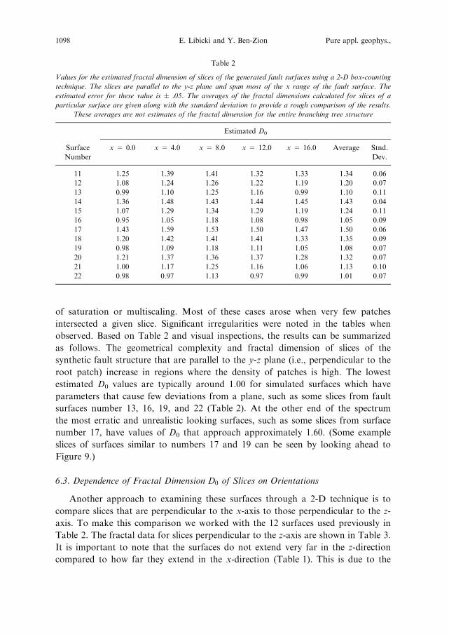
of saturation or multiscaling. Most of these cases arose when very few patches

intersected a given slice. Significant irregularities were noted in the tables when

observed. Based on Table 2 and visual inspections, the results can be summarized

as follows. The geometrical complexity and fractal dimension of slices of the

synthetic fault structure that are parallel to the y-z plane (i.e., perpendicular to the

root patch) increase in regions where the density of patches is high. The lowest

estimated D0 values are typically around 1.00 for simulated surfaces which have

parameters that cause few deviations from a plane, such as some slices from fault

surfaces number 13, 16, 19, and 22 (Table 2). At the other end of the spectrum

the most erratic and unrealistic looking surfaces, such as some slices from surface

number 17, have values of D0 that approach approximately 1.60. (Some example

slices of surfaces similar to numbers 17 and 19 can be seen by looking ahead to

Figure 9.)

6.3. Dependence of Fractal Dimension D0 of Slices on Orientations

Another approach to examining these surfaces through a 2-D technique is to

compare slices that are perpendicular to the x-axis to those perpendicular to the z-

axis. To make this comparison we worked with the 12 surfaces used previously in

Table 2. The fractal data for slices perpendicular to the z-axis are shown in Table 3.

It is important to note that the surfaces do not extend very far in the z-direction

compared to how far they extend in the x-direction (Table 1). This is due to the

Table 2

Values for the estimated fractal dimension of slices of the generated fault surfaces using a 2-D box-counting

technique. The slices are parallel to the y-z plane and span most of the x range of the fault surface. The

estimated error for these value is � .05. The averages of the fractal dimensions calculated for slices of a

particular surface are given along with the standard deviation to provide a rough comparison of the results.

These averages are not estimates of the fractal dimension for the entire branching tree structure

Estimated D0

Surface

Number

x = 0.0 x = 4.0 x = 8.0 x = 12.0 x = 16.0 Average Stnd.

Dev.

11 1.25 1.39 1.41 1.32 1.33 1.34 0.06

12 1.08 1.24 1.26 1.22 1.19 1.20 0.07

13 0.99 1.10 1.25 1.16 0.99 1.10 0.11

14 1.36 1.48 1.43 1.44 1.45 1.43 0.04

15 1.07 1.29 1.34 1.29 1.19 1.24 0.11

16 0.95 1.05 1.18 1.08 0.98 1.05 0.09

17 1.43 1.59 1.53 1.50 1.47 1.50 0.06

18 1.20 1.42 1.41 1.41 1.33 1.35 0.09

19 0.98 1.09 1.18 1.11 1.05 1.08 0.07

20 1.21 1.37 1.36 1.37 1.28 1.32 0.07

21 1.00 1.17 1.25 1.16 1.06 1.13 0.10

22 0.98 0.97 1.13 0.97 0.99 1.01 0.07

1098 E. Libicki and Y. Ben-Zion Pure appl. geophys.,

Figure 7

Three estimates of fractal dimension of simulated structures using box-counting methods. (a) A linear plot

for the box-counting method of a slice of a branching structure giving an estimated fractal dimension of

1.25. (b) A case where there is saturation for larger box sizes as seen by the plot leveling off at higher side

length values (gray data points are not included in the best-fit line). (c) A linear plot of estimated fractal

dimension with a 3-D box-counting technique discussed later but included here for comparison. In general,

the closer R2 (the coefficient of determination) is to 1.0 the better the line fit.

Vol. 162, 2005 Stochastic Branching Models of Fault Surfaces 1099

typically small amounts of rotation that keep the faults usually growing in the x and

y directions. This limits how far the slices can be from the origin in the z-direction. A

brief examination indicates that any comparisons will be difficult for a variety of

reasons. First, there is the problem that most of the surfaces stay close to the z = 0

plane. Second, even when surfaces do stray at least a few units from z = 0, they are

usually limited to only a small number of patches. As shown in Table 3, this tends to

produce plots with either significant saturation or data sets that are not necessarily

linear. However, even with these difficulties there are at least two interesting

observations that can still be made. The first point is illustrated by direct visual

comparison in Figure 8. The x-slices tend to create patterns that have many branches

but few gaps, whereas the z-slices tend to create the opposite effect and usually show

little branching but quite a few gaps. The second point is that the fractal dimensions

estimated for the x-slices and z-slices seem to reach similar values for the same fault

surface. However, it is important to note that the scales for each direction are quite

different. It thus appears that these surfaces are best described as self-affine rather

than self-similar, which is not surprising since natural fault structures tend to have

preferred orientations.

Table 3

Values for the estimated fractal dimension of slices of the generated fault surfaces using a 2-D box-counting

technique. The slices are parallel to the x-y plane and span most of the z range of the fault surfaces. The

estimated error for these value is � .05. The averages of the fractal dimensions calculated for slices of a

particular surface are given along with the standard deviation to provide a rough comparison of the results.

These averages are not estimates of the fractal dimension for the entire branching tree structure

Estimated D0

Surface

Number

z = )2.0 z = )1.0 z = 1.0 z = 2.0 Average Stnd.

Dev.

11 1.14 1.34 1.30 1.22** 1.25 0.09

12 0.94* 1.08* 1.11** 1.06** 1.05 0.07

13 0.87* 0.99** 0.92 1.01** 0.95 0.06

14 1.28 1.50 1.28 1.22 1.32 0.12

15 X 0.98** 1.08** 1.02* 1.03 0.05

16 X X 1.00 X 1.00 NA

17 1.55 1.62 1.55 1.44 1.54 0.07

18 X 0.97 1.16 1.04* 1.06 0.10

19 X X X X NA NA

20 0.96 1.05* 1.18 1.27* 1.12 0.14

21 X 0.84* 0.98 1.00 0.94 0.09

22 X X X X NA NA

X — The fractal dimension is not applicable since the surface does not pass through the location.* — Extra points were removed (usually those representing the larger box sizes) since significant saturation

occurred for more than just the two points at either end of the scale.** — Contains either a bend, significant curvature, or points that significally deviate from the line, and thus

it may not be best to fit a line to these data sets. Appears to be caused when only a small portion of the

surface passes through the slice.

1100 E. Libicki and Y. Ben-Zion Pure appl. geophys.,

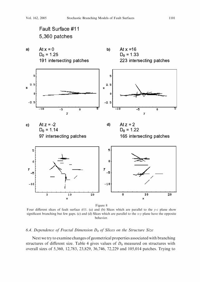
6.4. Dependence of Fractal Dimension D0 of Slices on the Structure Size

Nextwe try to examine changes of geometrical properties associatedwith branching

structures of different size. Table 4 gives values of D0 measured on structures with

overall sizes of 5,360, 12,783, 23,829, 36,746, 72,229 and 105,014 patches. Trying to

Figure 8

Four different slices of fault surface #11. (a) and (b) Slices which are parallel to the y-z plane show

significant branching but few gaps. (c) and (d) Slices which are parallel to the x-y plane have the opposite

behavior.

Vol. 162, 2005 Stochastic Branching Models of Fault Surfaces 1101

compare surfaces with different overall size is not straightforward because different size

trees use different seeds for the random number generators, leading to the creation of

different branching structures. If values of the fractal dimension were the same

throughout an entire structure it would be simple to compare, but since they are not it is

unclear how to make representative comparisons. Making a comparison at x = 0.0

Table 4

Values for the estimated fractal dimension of slices of different size fault surfaces using a 2-D box-counting

technique. The slices are parallel to the y-z plane taken at x= 0.0 and x= 8.0. The estimated error for these

values is � .05

Estimated D0 Estimated D0

Surface

Number

Patches x = 0.0 x = 8.0 Surface

Number

Patches x = 0.0 x = 8.0

11 5,360 1.25 1.41 17 5,360 1.43 1.53

31 12,783 1.20 1.47 37 12,783 1.33 1.57

51 23,829 1.47 1.45 57 23,829 1.60 1.43

71 36,746 1.39 1.23 77 36,746 1.41 1.46

91 72,229 1.46 1.46 97 72,229 1.58 1.62

111 105,014 1.58 1.63 117 105,014 1.71 1.61

12 5,360 1.08 1.26 18 5,360 1.20 1.41

32 12,783 1.20 1.34 38 12,783 1.31 1.42

52 23,829 1.38 1.39 58 23,829 1.38 1.34

72 36,746 1.42 1.39 78 36,746 1.35 1.38

92 72,229 1.34 1.43 98 72,229 1.48 1.55

112 105,014 1.51 1.47 118 105,014 1.56 1.46

13 5,360 0.99 1.25 19 5,360 0.98 1.18

33 12,783 1.20 1.28 39 12,783 1.08 1.15

53 23,829 1.22 1.24 59 23,829 1.16 1.12

73 36,746 1.20 1.29 79 36,746 1.10 1.11

93 72,229 1.25 1.33 99 72,229 1.12 1.13

113 105,014 1.43 1.45 119 105,014 1.28 1.24

14 5,360 1.36 1.43 20 5,360 1.21 1.36

34 12,783 1.23 1.51 40 12,783 1.25 1.39

54 23,829 1.54 1.50 60 23,829 1.44 1.38

74 36,746 1.44 1.46 80 36,746 1.40 1.44

94 72,229 1.60 1.42 100 72,229 1.44 1.48

114 105,014 1.61 1.48 120 105,014 1.61 1.52

15 5,360 1.07 1.34 21 5,360 1.00 1.25

35 12,783 1.26 1.36 41 12,783 1.21 1.24

55 23,829 1.28 1.32 61 23,829 1.23 1.22

75 36,746 1.28 1.32 81 36,746 1.14 1.20

95 72,229 1.35 1.42 101 72,229 1.28 1.31

115 105,014 1.45 1.39 121 105,014 1.31 1.36

16 5,360 0.95 1.18 22 5,360 0.98 1.13

36 12,783 1.09 1.11 42 12,783 0.99 1.05

56 23,829 1.16 1.14 62 23,829 1.10 1.07

76 36,746 1.11 1.11 82 36,746 1.00 1.00

96 72,229 1.13 1.12 102 72,229 1.01 1.00

116 105,014 1.26 1.21 122 105,014 1.13 1.08

1102 E. Libicki and Y. Ben-Zion Pure appl. geophys.,

might be informative since the root disk causes all the faults to pass through x = 0.0.

The results of Table 4 suggest a general trend towards an increasing D0 value with

increasing size, as expected from the corresponding tendency for more intersecting

disks. The comparison shows that for variables causing the most planar surfaces the

estimated dimensions change little with increasing size, whereas the more complex

structures tend to become quite disordered at large sizes (Fig. 9). The general validity of

this comparison is unknown, since the nonrandom placement of the root may have

significant influence on the geometry of the fault for the earliest created patches, which

are often located near the plane x = 0.0. For this reason, we also compare results for

different size faults at the plane x=8.0, which is both away from the root patch and at a

location where significant portions of all the faults pass through. As seen in Table 4

there is a weak correlation at best between tree size and fractal dimension at x = 8.0.

The generality of this result is again not clear since the different size faults at a given

location should be uncorrelated due to the randomness except for possibly near x =

0.0. It appears that a representative comparison between estimated fractal values of

faults of different sizes requires calculating a fractal dimension of the entire branching

structure rather than slices. Such an approach will be discussed later.

It is interesting to examine the evolution of geometrical properties of a branching

tree as the structure grows with ‘‘time.’’ The time may be represented by the

generation index, which is equivalent to having 1 unit of time pass from every

generation to the next. This, however, would not take into consideration the different

number of patches created at each generation or changes to the growth rate over

time. A second possibility is to consider the tree at different stages along its growth,

i.e., the surface could be examined after all additional m patches were added to the

structure. This would be most effective if the entire structure was being examined.

However, since the current focus is on slices of the structure, we represent growth by

analyzing the slices after every n patches passed through the particular slice being

examined. An additional decision to be made is whether to use ‘‘time windows’’ (e.g.,

examining patches 1–50, 51–100, etc.) or to analyze the entire surface up to that point

(e.g., examining patches 1–50, 1–100, etc.). Since mechanical effects such as

smoothing with ongoing slip (and hence time), erosion, etc., are ignored, the latter

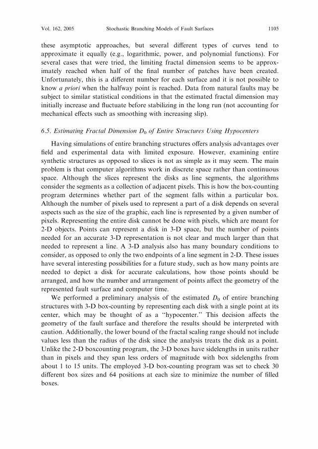
approach was used. Figure 10 gives an example of how these surfaces evolve during

growth. Notice that there is a tendency for the surface to spread outwards along the

y-z plane over time, although the surface also frequently backtracks onto itself.

Some example results on the change in D0 versus the growth of the fault are

presented in Figure 11. Somewhat unexpectedly, the estimated fractal dimension

tends to level off in each case and the values are generally approached asymptotically.

This is somewhat similar to results on fractal dimension of (relatively high resolution)

observed hypocenter data of ROBERTSON et al. (1995). There are fluctuations from a

smooth curve with the major deviations at the beginning. This is probably a

statistical effect associated with the limited number of patches in a particular area

(especially at the beginning). It would be useful to have a curve fit that approximates

Vol. 162, 2005 Stochastic Branching Models of Fault Surfaces 1103

Figure 9

A comparison of the persistence (or lack thereof) of surfaces when using the more extreme parameter

values. Panels (a) and (b) have too much branching whereas (c) and (d) are essentially planar.

1104 E. Libicki and Y. Ben-Zion Pure appl. geophys.,

these asymptotic approaches, but several different types of curves tend to

approximate it equally (e.g., logarithmic, power, and polynomial functions). For

several cases that were tried, the limiting fractal dimension seems to be approx-

imately reached when half of the final number of patches have been created.

Unfortunately, this is a different number for each surface and it is not possible to

know a priori when the halfway point is reached. Data from natural faults may be

subject to similar statistical conditions in that the estimated fractal dimension may

initially increase and fluctuate before stabilizing in the long run (not accounting for

mechanical effects such as smoothing with increasing slip).

6.5. Estimating Fractal Dimension D0 of Entire Structures Using Hypocenters

Having simulations of entire branching structures offers analysis advantages over

field and experimental data with limited exposure. However, examining entire

synthetic structures as opposed to slices is not as simple as it may seem. The main

problem is that computer algorithms work in discrete space rather than continuous

space. Although the slices represent the disks as line segments, the algorithms

consider the segments as a collection of adjacent pixels. This is how the box-counting

program determines whether part of the segment falls within a particular box.

Although the number of pixels used to represent a part of a disk depends on several

aspects such as the size of the graphic, each line is represented by a given number of

pixels. Representing the entire disk cannot be done with pixels, which are meant for

2-D objects. Points can represent a disk in 3-D space, but the number of points

needed for an accurate 3-D representation is not clear and much larger than that

needed to represent a line. A 3-D analysis also has many boundary conditions to

consider, as opposed to only the two endpoints of a line segment in 2-D. These issues

have several interesting possibilities for a future study, such as how many points are

needed to depict a disk for accurate calculations, how those points should be

arranged, and how the number and arrangement of points affect the geometry of the

represented fault surface and computer time.

We performed a preliminary analysis of the estimated D0 of entire branching

structures with 3-D box-counting by representing each disk with a single point at its

center, which may be thought of as a ‘‘hypocenter.’’ This decision affects the

geometry of the fault surface and therefore the results should be interpreted with

caution. Additionally, the lower bound of the fractal scaling range should not include

values less than the radius of the disk since the analysis treats the disk as a point.

Unlike the 2-D boxcounting program, the 3-D boxes have sidelengths in units rather

than in pixels and they span less orders of magnitude with box sidelengths from

about 1 to 15 units. The employed 3-D box-counting program was set to check 30

different box sizes and 64 positions at each size to minimize the number of filled

boxes.

Vol. 162, 2005 Stochastic Branching Models of Fault Surfaces 1105

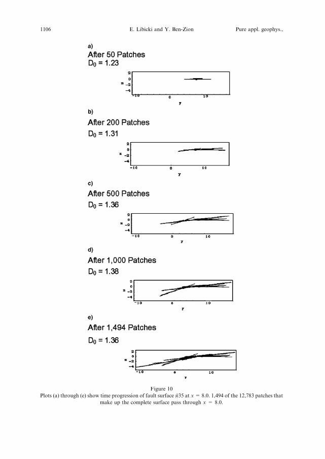
Figure 10

Plots (a) through (e) show time progression of fault surface #35 at x= 8.0. 1,494 of the 12,783 patches that

make up the complete surface pass through x = 8.0.

1106 E. Libicki and Y. Ben-Zion Pure appl. geophys.,

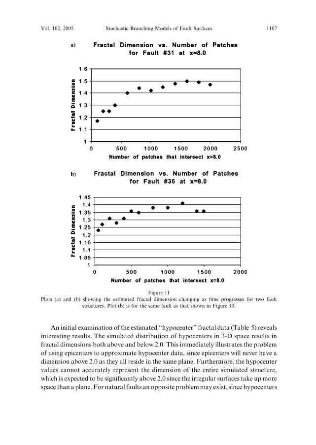
An initial examination of the estimated ‘‘hypocenter’’ fractal data (Table 5) reveals

interesting results. The simulated distribution of hypocenters in 3-D space results in

fractal dimensions both above and below 2.0. This immediately illustrates the problem

of using epicenters to approximate hypocenter data, since epicenters will never have a

dimension above 2.0 as they all reside in the same plane. Furthermore, the hypocenter

values cannot accurately represent the dimension of the entire simulated structure,

which is expected to be significantly above 2.0 since the irregular surfaces take upmore

space than a plane. For natural faults an opposite problemmay exist, since hypocenters

Figure 11

Plots (a) and (b) showing the estimated fractal dimension changing as time progresses for two fault

structures. Plot (b) is for the same fault as that shown in Figure 10.

Vol. 162, 2005 Stochastic Branching Models of Fault Surfaces 1107

of small events (which comprise the bulk of the data) tend to be located aroundplaces of

geometrical complexities (e.g., segment offsets). This may lead to a bias toward higher

dimension than that representing the entire structure.

The estimated 3-D box-counting dimensions currently do not have a clear

relationship to their 2-D counterparts, though the obtained fractal values tend to

decrease as the faults become more planar and tend to increase with increasing fault

size. How fast the calculated values approach stable values as more points are used to

represent each patch, and how well other fractal measures compare to the values in

Table 5 are important questions that are left for future work.

7. Concluding Remarks

This paper examines assumptions associated with the geometric stochastic

branching model of KAGAN (1982) based on earlier work of VERE-JONES (1976,

1977), and uses a version of the model to simulate branching structures with different

sets of parameters. The results highlight some non-uniqueness issues of the model,

manifested by different sets of parameters creating similar surfaces. The simulated

structures are used to asses the validity of characterizing the geometry of irregular

rough surfaces with typical fractal measurements. This could have been done with

several possible approaches, including focusing onone ormoremethods for calculating

fractal dimensions, one or more aspects of the surface to measure (e.g. hypocenters or

fault traces, etc.). The approach taken here was to look at many different aspects of the

synthetic surfaces, using primarily the 2-D box-counting technique.

The performed simulations and analysis provide insights into calculations of

fractal dimensions of fault surfaces, although some concerns with the model and

analysis should be addressed further. One issue is that the model surface is composed

of many small circular patches that cannot share sides to form a continuous surface.

The patches often overlap and intersect many times, reducing the ability of the model

to represent a physical object. Using alternate shapes for the patches such as a square

would avoid this problem since they could be placed adjacent to each other and share

an entire side. However, squares would cause different problems since they have a

small number of axes of symmetry. The shape of a patch should have little relevance

when the patches are small enough to avoid discretization effects. We note, however,

that with 5,000 patches and even with 105,000 there may still be discretization effects,

since the (2-unit) diameter of a patch can be a significant percentage of the full length

of the surface. Other issues involve whether the stochastic branching model provides

a good representation of natural fault surfaces and the various simplifying

assumptions of the branching model. For example, the parameter k of the Poisson

distribution was set equal to 1.0 regardless of the state of the structure. A more

physical assumption would be to increase k with increasing fault size to represent the

dependency of stress concentration on the failure size. Another possible modification

1108 E. Libicki and Y. Ben-Zion Pure appl. geophys.,

Table

5

Values

fortheestimatedfractaldim

ensionofthepatchcenters

ofthegeneratedfaultsurfacesusinga3-D

box-countingtechnique.

Theestimatederrorforthese

values

is�

0.01

Fault

Surface

Number

D0

Fault

Surface

Number

D0

Fault

Surface

Number

D0

Fault

Surface

Number

D0

Fault

Surface

Number

D0

Fault

Surface

Number

D0

11

1.83

31

2.00

51

2.04

71

2.04

91

2.12

111

2.23

12

1.73

32

1.95

52

1.94

72

1.97

92

2.07

112

2.14

13

1.75

33

1.93

53

1.87

73

1.82

93

1.95

113

1.94

14

1.95

34

2.03

54

2.02

74

2.02

94

2.10

114

2.16

15

1.76

35

1.97

55

1.88

75

1.91

95

1.95

115

2.01

16

1.69

36

1.80

56

1.75

76

1.73

96

1.75

116

1.84

17

1.97

37

2.03

57

2.16

77

2.08

97

2.17

117

2.25

18

1.78

38

1.99

58

1.91

78

1.93

98

2.07

118

2.07

19

1.69

39

1.78

59

1.76

79

1.74

99

1.77

119

1.75

20

1.79

40

1.97

60

1.96

80

2.00

100

2.04

120

2.05

21

1.68

41

1.85

61

1.84

81

1.75

101

1.83

121

1.90

22

1.67

42

1.77

62

1.72

82

1.73

102

1.75

122

1.74

Vol. 162, 2005 Stochastic Branching Models of Fault Surfaces 1109

would be to replace the Poisson distribution with a distribution that does not assume

independence of different structural elements from previous history and each other.

Whether or not the model provides a good representation of natural fault

surfaces, some of the lessons learned about analysis of fractal dimensions should

apply to natural objects. For example, the results indicate that properties of 2-D

slices of an irregular object vary and are not easily related to the overall volumetric

object. This implies that the subsurface structure of a fault is unlikely to have a

simple relation to its surface trace. Similarly, assuming that the geometry of a fault

surface is represented adequately by a sparse cloud of hypocenter points is not

justified, even in the absence of location errors.

The value of using fractal dimensions to characterize earthquake fault geometry

is currently unclear. Two objectives for future work are to fully characterize the

comparability of different fractal techniques and to determine how much information

can actually be gathered by using such techniques on irregular surfaces.

Acknowledgments

We thank Yan Kagan for discussions in early stages of the work and Shoshana

Levin for the 3-D box-counting program used in section 6.5. The paper benefited

from many useful comments by Yan Kagan, David Vere-Jones and two anonymous

referees. The study was supported by a Zumberge research fund of USC.

REFERENCES

BEN-ZION, Y., Appendix 2, Key formulas in earthquake seismology. In: International Handbook of

Earthquake and Engineering Seismology, Part B, 1857–1875 (Academic Press, 2003).

BEN-ZION, Y. and LYAKHOVSKY, V. (2002), Accelerated Seismic Release and Related Aspects of Seismicity

Patterns on Earthquake Faults, Pure Appl. Geophys. 159, 2385–2412.

BEN-ZION, Y. and SAMMIS, C.G. (2003), Characterization of Fault Zones, Pure Appl. Geophys. 160, 677–

715.

ENEVA, M. (1994), Monofractal or Multifractal: A Case Study of Spatial Distribution of Mining Induced

Seismic Activity, Nonlinear Processes in Geophys. 1, 182–190.

FISHER, D.S., DAHMEN, K., RAMANATHAN, S., and BEN-ZION, Y. (1997), Statistics of Earthquakes in

Simple Models of Heterogeneous Faults, Phys. Rev. Lett. 78, 4885–4888.

FROHLICH, C. and DAVIS, S.D. (1993), Teleseismic b Values; or, Much Ado About 1.0, J. Geophys. Res. 98,

631–644.

GOLTZ, C., Fractal and Chaotic Properties of Earthquakes (Springer, Berlin 1997).

GONZATO, G., MULARGIA, F., and MARZOCCHI, W. (1998), Practical Applications of Fractal Analysis:

Problems and Solutions, Geophys. J. Int. 132, 275–282.

GONZATO, G., MULARGIA, F., and CICCOTTI, M. (2000), Measuring the Fractal Dimension of Ideal and

Actual Objects: Implications for Application in Geology and Geophysics, Geophys. J. Int. 142, 108–116.

GUTENBERG, B. and RICHTER, C.F., Seismicity of the Earth and Associated Phenomena (2nd edition)

(Princeton University Press, Princeton, N.J. 1954).

GUTENBERG, B. and RICHTER, C.F. (1956), Magnitude and Energy of Earthquakes, Ann. Geofis. 9, 1–15.

1110 E. Libicki and Y. Ben-Zion Pure appl. geophys.,

HARRIS, T. E., The Theory of Branching Process (Springer-Verlag, Berlin 1963).

HARTE, D., Multifractals: Theory and Applications (Chapman and Hall/CRC, Boca Raton 2001).

HIRATA, T. (1989), Fractal Dimension of Fault Systems in Japan: Fractal Structure in Rock Fracture

Geometry at Various Scales, Pure Appl. Geophys. 131, 157–170.

KAGAN, Y.Y. (1982), Stochastic Model of Earthquake Fault Geometry,Geophy. J.R. astr. Soc. 71, 659–691.

KAGAN, Y.Y. (1990), Random Stress and Earthquake Statistics: Spatial Dependence, Geophys. J. Int. 102,

573–583.

KAGAN, Y.Y. (1994), Observational Evidence for Earthquakes as a Nonlinear Dynamic Process, Physica D

77, 160–192.

KARLIN, S. and TAYLOR, H.M., A First Course in Stochastic Processes (Academic Press, San Diego 1975).

LAWLER, G.F., Introduction to Stochastic Processes (Chapman and Hall/CRC, Boca Raton 1995, reprinted

2000).

LEON-GARCIA, A., Probability and Random Processes for Electrical Engineering (Addison-Wesley

Publishing Company, Reading Massachusetts 1994).

LYAKHOVSKY, V., BEN-ZION, Y., and AGNON, A. (2001), Earthquake Cycle, Fault Zones, and Seismicity

Patterns in a Rheologically Layered Lithosphere, J. Geophys. Res. 106, 4103–4120.

MALCAI, O., LIDAR, D.A., BIHAM, O., and AVNIR, A. (1997), Scaling Range and Cutoffs in Empirical

Fractals, Phys. Rev. E 56, 2817–2828.

OKUBO, P.G. and AKI, K. (1987), Fractal Geometry in the San Andreas Fault System, J. Geophys. Res. 92,

345–355.

PRESS, W.H., TEUKOLSKY, S.A., VETTERLING, W.T., and FLANNERY, B.P., Numerical Recipes in Fortran 90

(Cambridge University Press, Cambridge 1996).

RICE, J.A., Mathematical Statistics and Data Analysis (2nd edition) (Duxbury Press, Belmont California

1995).

ROBERTSON, M.C., SAMMIS, C.G., SAHIMI, M., and MARTIN, A.J. (1995), Fractal Analysis of Three-

dimensional Spatial Distributions of Earthquakes with a Percolation Interpretation, J. Geophys. Res. 100,

609–620.

SCHROEDER, M., Fractals, Chaos, Power Laws (W. H. Freeman and Co., New York 1991).

TURCOTTE, D. L., Fractals and Chaos in Geology and Geophysics (Cambridge University Press, Cambridge

1997).

VERE-JONES, D. (1976), A Branching Model for Crack Propagation, Pure Appl. Geophys. 114, 711–725.

VERE-JONES, D. (1977), Statistical Theories of Crack Propagation, Math. Geol. 9, 455–481.

(Received August 30, 2003, accepted July 20, 2004)

To access this journal online:

http://www.birkhauser.ch

Vol. 162, 2005 Stochastic Branching Models of Fault Surfaces 1111