Stochastic actor-oriented models for networkchange 1

Tom A.B. Snijders 2

University of Groningen

1996

1Published in Journal of Mathematical Sociology 21 (1996), 149–172.2The ideas presented in this paper benefited from discussions with many people

at the ICS, of whom I wish to mention Frans Stokman, Evelien Zeggelink, andRoger Leenders.

Abstract

A class of models is proposed for longitudinal network data. These modelsare along the lines of methodological individualism: actors use heuristics totry to achieve their individual goals, subject to constraints. The current net-work structure is among these constraints. The models are continuous timeMarkov chain models that can be implemented as simulation models. Theyincorporate random change in addition to the purposeful change that followsfrom the actors’ pursuit of their goals, and include parameters that must beestimated from observed data. Statistical methods are proposed for estimat-ing and testing these models. These methods can also be used for parameterestimation for other simulation models. The statistical procedures are basedon the method of moments, and use computer simulation to estimate thetheoretical moments. The Robbins-Monro process is used to deal with thestochastic nature of the estimated theoretical moments. An example is givenfor Newcomb’s fraternity data, using a model that expresses reciprocity andbalance.

Keywords: methodological individualism; Markov process; Newcomb data;balance; Robbins-Monro process; simulation models; method of moments;simulated moments; random utility.

1 Introduction: the integration of theoretical

and statistical model

Empirical tests of sociological theories are usually based on the following lineof procedure: (1) verbal (sometimes mathematical) representations of thetheory; (2) deductions of associations between certain variables that expresscrucial concepts in the theory, or of other qualitative relations; (3) the em-pirical test of these qualitative relations within a statistical framework. Thelatter incorporates (if it is adequate) the operationalisation of the focal andother relevant variables as well as the data collection methods, but does notmake direct reference to the tested theory. E.g., the theory is shown to implythat within population P , variables A and B are positively associated whencontrolling for variables C to F, and a partial correlation is tested withinthe explicit or implicit statistical framework of a random sample from apopulation in which several variables are observed, having an approximatelymultivariate normal distribution.

This approach is useful but not the only possibility. It would be preferablethat the verbal or mathematical deductions of the theory’s implications beintegrated with the statistical model that is used for the empirical test. Suchan integration leads to a statistical model that is itself a direct expression ofthe sociological theory. Econometric models of choice among a finite set ofpossibilities, proposed by McFadden and others since the 1970’s (see McFad-den 1973, Maddala 1983, Pudney 1989), provide an example. Other examplesare the models of optimizing agents presented by Chow (1983, Chapter 12)and the model of the production of collective goods proposed by Snijders,Van Dam and Weesie (1994). The integration of theoretical and statisticalmodel is more complicated but it can lead to more stringent theory develop-ment because it requires a completely explicit theory and provides a muchmore direct test of the theory.

This paper presents the outline, and a relatively simple example, of suchtheoretical-cum-statistical models for evolution of networks. These modelsrefer to the evolution of the relation network and of individual behavior ina (non-changing) set of actors, and are based on the assumption that eachactor has his or her own goals which he/she tries to advance in accordanceto his/her constraints and possibilities. Delopment of networks is consid-ered rather than observations of networks at a single time point, because

1

single observations of networks will usually contain too little information fora substantial empirical test of a theory. The approach is methodologicallyindividualistic: the driving force behind the network dynamics is constitutedby the actors’ actions; each actor takes actions in order to further his owngoals; these actions are in the domain of his own behavior or of the directedrelationships from him to others; the actors are constrained by their socialenvironment.

In order that theoretical models can be empirically tested, they must(implicitly or explicitly) contain a stochastic, or random, element; after all,human behavior and social phenomena are so complex that any theory canexplain such phenomena only partially, or approximately, and the inclusionin the model of a stochastic element is desirable to account for the non-explained part of empirical observations. Therefore, probabilistic modelsand, more specifically, random utility models, are needed for the integrationof theoretical and empirical modeling.

In the following we mention some approaches to dynamical network mod-eling that have been presented in the literature. This is far from an exhaustivereview, but merely serves to point out some of the work that has providedinspiration for this paper.

Most network models for which statistical inference procedures have beendeveloped (a review is given by Wasserman and Faust, 1994), are almost triv-ial from the point of view of sociological theory. The reason is the need tokeep these models mathematically tractable in order to apply conventionalstatistical methods. E.g., the p1 model proposed by Holland and Leinhardt(1981) (see Wasserman and Faust, op. cit., for further literature on thismodel), which may be the most extensively developed network model todate as far as procedures for statistical inference are concerned, is a modelin which dyads (i.e., the constellation of relations between pairs of actors)are statistically independent of each other. The assumption of independencebetween dyads excludes a priori almost all sociologically interesting interac-tions.

Conditionally uniform models, of which a great variety was mentioned byHolland and Leinhardt (1976), do allow a modicum of dependence betweendyads; but they take into account only the total number and the degree ofmutuality of choices, in some models combined with in- and out-degrees (seeSnijders, 1991). As a consequence, conditionally uniform models can serve at

2

best as null models against which to test sociological theories. This is exactlywhat Holland and Leinhardt (1976 and later publications) propose. Theirprocedure to test a given theory is the following: use as the null hypothesisthe conditionally uniform U |M, A, N model, which considers a network withgiven total number of choices and a given number of mutual choices; expressthe theory in the test statistic (such as Holland and Leinhardt’s τ -statistic,which is a linear function of the triad census). Such a testing procedure isepistemologically weak. A rejection of the null hypothesis (which is all theresearcher can hope for within the framework of this procedure) indicatesthat either the test statistic is larger than expected under the null hypothesis(defined by the U |M, A, N distribution), or something rather improbable(an error of the first kind) has happened. However, this implies quite weaksupport for the substantive theory, because the null hypothesis is so crudethat it would contradict any non-trivial sociological theory. What is needed isa mathematical model for the alternative rather than for the null hypothesis.

The dynamic Markov models for networks (Holland and Leinhardt 1977,Wasserman 1977, 1981, Mayer 1984, Leenders 1994) offer more scope for ex-pressing sociological theories. Except for Mayer (1984), these models assumeconditional independence between dyads. The assumption of conditionallyindependent dyads is a strong restriction. Most serious sociological theorieswill imply some kind of dependence structure between different dyads. Thesemodels can be seen as statistical models, not directly derived from a socio-logical theory, but in other aspects closely related to the models proposed inthis paper.

The research tradition on biased nets that started with Rapoport (1951,1957) and was continued, a.o., by Fararo (1981), Fararo and Skvoretz (1984,1994), and Skvoretz (1991), is an interesting approach to modeling varioussubstantively important effects in networks, such as transitivity, subgroupformation, etc., but still leaves a gap between theoretical mathematical mod-els and data analysis. These authors have developed theoretical models,and used existing statistical models for data analysis. In the terminology ofSkvoretz (1991, p. 277), what the present paper aims to do is the integrationof theoretical and methodological models.

Zeggelink (1993, 1994, 1995) developed rational choice-based models forfriendship formation in networks. The dynamical part of these models israther weak in the sense that insights and ideas about dynamical networkevolution are used in view of yielding an acceptable equilibrium situation

3

rather than in view of providing an acceptable description of the dynamicalprocess itself. Moreover, these models also still lack statistical estimationand testing methods.

Stokman and Zeggelink (1993) proposed a model for the evolution ofpolicy positions of actors in policy networks and for the resulting collectiveoutcomes. The actors can exhibit policy positions and can establish rela-tions with other actors. Their choice among the possible actions is based ontheir expectation of the utility that will result from the actions. This modelis theoretically more sophisticated than the one presented in Section 4 ofthe present paper, but it lacks procedures for statistical estimation and test-ing. This is related to the fact that this model (like practically all availablemodels) does not allow for stochastic deviations between expected model out-comes and observed outcomes. Admitting such deviations in the model is anessential requirement for the development of statistical testing procedures.

The stochastic models for network dynamics that are meaningful as anexpression of substantive theory are so complicated that the developmentfor these models of statistical methods along classical lines (e.g., maximumlikelihood estimators, minimum variance unbiased estimators, likelihood ra-tio tests) is difficult and in many cases seems to border on the impossible.Computer simulation, on the other hand, of these models often is quite feasi-ble. It will be shown below that computer simulation opens the possibility of(computer-intensive) methods of statistical inference, although these meth-ods are not necessarily optimal in a statistical sense. The focus of this paperis on the presentation of a class of theory-based stochastic dynamic modelsfor networks, and of simulation-based statistical methods to estimate andtest the associated parameters. As an example, Newcomb’s (1961) fraternitydata will be used.

The models proposed in this paper are Markov chain models with a con-tinuous time parameter, observed at discrete time points. Such models wereproposed for social networks by Holland and Leinhardt (1977), and elabo-rated by Wasserman (1977, 1979, 1980), Mayer (1984), and Leenders (1994).An obstacle in the development and application of continuous time Markovmodels has been the difficulty of deriving statistical methods for models thatgo beyond dyad independence. In the present paper this obstacle is overcomeby using non-traditional statistical methods, sacrificing some computer timeand some statistical efficiency, but providing possibilities for the statisticalanalysis of a large class of dynamic network models.

4

2 Elements of stochastic actor-oriented net-

work models

In this section we propose a class of dynamic network models. In these modelsthe evolution of the network is the result of the actions of the individual actorsin the network, each of whom is individually optimizing his or her own utility,given the constraints determined by the network and, possibly, by externalinfluences. Such models can be used, e.g., in rational choice approaches tosocial network evolution. These models combine utility theory and Markovprocesses, and are close in theoretical spirit to the models for adaptivelyrational action reviewed by Fararo (1989, Sections 3.5-3.6). What is new inthem is the incorporation of parameters that are not known a priori but canbe estimated from data, and the allowance for unexplained change. Thesecomponents are necessary for a fusion of theoretical with statistical modeling.

First, the ingredients for the model are conceptually introduced. Thensome of these ingredients are further specified. A concrete example will begiven in Section 4.

The outcome space for our dynamic network model has the following basiccomponents.

• The time parameter t. It is represented as a continuous parameter.The time axis is denoted T .

• The set of actors. In this paper a fixed and finite set of actors isconsidered; addition of new actors, or exit from the network, will notbe taken into consideration. The set of actors is denoted G, the numberof actors by g.

• The network of relations between the actors. All relations consideredare directed relations (e.g., liking, esteem or influence) because of theapproach of methodological individualism. Relations commonly con-sidered as undirected relations, such as friendship or cooperation, willbe regarded as mutual directed relationships. Relations may be single,but it is more interesting to consider multiple and/or valued relations.(This will be elaborated in later papers.) Relationships between actorsmay change over time, and may be determined by the social structure(e.g., hierarchy or kinship constraints) but it is more interesting when

5

the relationships can be purposely changed by the authors. The rela-tion network is indicated by the time-dependent matrix F (t) for t ∈ T .If the relationship pattern is represented by a directed graph, F (t) canbe taken as the adjacency matrix. The space of possible relation net-works is indicated by F ; this can be the space of directed graphs on gvertices, but also a more complicated space.

• Attributes for the actors can be included in the model. These canbe stable (e.g., gender) or changeable (e.g., attitudes). Behavior orbehavior tendencies are also considered as changeable attributes. Whenthe number of attributes is q, with q ≥ 0, the values of the attributescan be represented by a time-dependent g × q matrix Z(t) for t ∈ T .For q = 0, there are no attributes.

The state of the model is the time-dependent value Y (t) = (F (t), Z(t)) ofnetwork and attributes. The stochastic model for the evolution of the networkwill be described using the following ingredients.

• The state of each actor, which is a function of the state of the model.It must be defined so that the actor’s evaluation of the state of themodel, in terms of his well-being, is a function only of his actor state.E.g., in a model of friendship networks, the state of an actor couldbe the number of his friends and the vector of their attributes. Thisconcept is not necessary for the construction of the model, but it isoften convenient.

• The information available to an actor. The actor must be informedin any case about his own state. It is possible, however, that theinformation available to the actor includes more than his own state.Just like the state of the actor, this is a model ingredient that is notnecessary but often convenient.

• Preference or utility functions for each actor, defined as a function ofthe information available to the actor. In principle, the preference func-tion is that which the actor tries to maximize. This is split in this paperinto a modeled component and a component that is known to the ac-tor but not to the researcher; the latter will be modeled as a randomcomponent.

6

The modeled components of the utility functions can be the same forall actors, but in more complicated models they may differ between ac-tors. Sometimes it is convenient to work with tension functions ratherthan preference functions. A tension function is a function which ac-tors wish to minimize. It is considered in this paper as equivalent to aconstant minus the modeled component of the utility function. Whenstarting with a bounded utility function, the tension function can bedefined as the maximum of the modeled component of the utility func-tion minus its present value. (Hoede (1990) and Zeggelink (1993) usetension functions in this way.) The tension function for actor i ∈ Gcan be represented as pi(Y ), where Y is the current state of the model.(In practice, pi will depend on suitable functions of Y , which can beinterpreted in terms of state and / or information.) The stochasticcomponent of the preference function will be treated further below, inthe discussion of the choice made by the actor, and the heuristic usedby him for this purpose.The tension function will usually not be completely known, but willcontain statistical parameters that have to be estimated from the avail-able data. E.g., in friendship networks, each actor may derive utilityfrom each relation partner based on the degree of perceived recipro-cation of positive affect and on the amount of support obtained; theweights of these two components could be free parameters in the sta-tistical model.

• The actions that an actor can take. Actions may refer to changeablerelations between the actors and others, and also to the changeableattributes of the actor. E.g., an action can be a change of opinion, achange of behavior tendency (such as to start smoking), a friendshipinvitation to another actor, or the acceptance of another actor’s invita-tion to a power contest. It is quite common that there exist constraintsin the social structure to the actions that an author can take.

• The time schedule indicating when it is possible to take certain actions.There may be constraints in the social structure as to when certain ac-tions are possible. In most cases, the model includes stochastic waitingtimes to indicate times for action.The rate of change over time will also be a statistical parameter in the

7

model, and estimated from the data.

• The choice made by an actor to perform a certain action (or to refrainfrom doing so when the opportunity is offered) depends on the actor’sexpectation of the utility of his state after the action. Ideally, the actorchooses the alternative for action that offers him the highest expectedutility.Two limitations to the principle of utility maximization are taken intoaccount, however. First, the modeled utility functions will not be aperfect representation of the actors’ utilities. Therefore, the utilitiesthat propel the actors’ choices also contain a random, i.e., unexplained,element. (Random utility models are commonly used in econometricmodeling; see, e.g., Maddala (1983) and Pudney (1989).) Second, anactor’s future state may depend also on future actions of others or onother things unknown to him; moreover, the actor’s capacity for strate-gic foresight and general calculations is bounded. Therefore, instead ofstrictly maximizing his expected utility, each actor uses a heuristic toapproximate the expected utility associated to each of the alternativesfor action available to him at a given moment. This heuristic is part ofthe model specification.

Some of these ingredients may be unobservable, others may be observable orobservable with a random error. In this paper, it is assumed that all relevantvariables are observed at a number of given time points. Models with latentvariables or with observation errors will be considered in later research.

Analogous to linear regression modeling, these longitudinal models haveto account for a degree of unexplained, or random change; the various the-oretical effects introduced must push back this random aspect and explainthe observed change to as large a degree as possible. In the process of modelbuilding, a sequence of increasingly complicated models can be fitted to thedata, starting with a null model of random change.

The outline given above can be further specified in such a way, thatthe resulting probability model is a Markov process in continuous time. Wedo not give an exposition of basic features of Markov processes, but referto the literature such as Chung (1967) or Karlin and Taylor (1975); and,for social network models, to Leenders (1994) and Wasserman (1977, 1979,1980). We only recall that a stochastic process {Y (t) | t ∈ T } is a Markov

8

process if for any time t0 ∈ T , the conditional distribution of the future,{Y (t) | t > t0} given the present and the past, {Y (t) | t ≤ t0}, is a functiononly of the present, Y (t0). Further, an event is said to happen at a rater, if the probability that it happens in a very short time interval (t, t + dt)is approximately equal to r dt. The reasons for specializing the model toMarkov processes are that such models often are quite natural, and thatthey lend themselves well for computer simulation. The resulting dynamiccomputer simulation models can be regarded as a type of discrete eventsimulation models as discussed by Fararo and Hummon (1994). In terms oftheir classification (op cit., p. 29), these models can have a categorical orcontinuous state space, they have a continuous parameter space and timedomain, the timing of events as well as the process generator are stochastic,and the dynamics are governed by probabilistic transition rules.

This further specification defines the time axis as T = {t | t ≥ 0}, andmakes the following assumptions about the time schedule.

• When, at a given time t, the state of the model is Y (t), the next actionby actor i will take place at a rate λi(Y (t)). This means that the waitingtime until the next action by actor i, if the state Y (t) does not changein the meantime, is a random variable with the negative exponentialdistribution, with expected value 1/λi(Y (t)). The time schedules of theactors are conditionally independent, given the state of the process; thisimplies that the waiting time until the next action by any actor hasthe exponential distribution with expected value 1/{∑i∈G λi(Y (t))}.

A second specification which is not necessary for the framework sketchedabove, but which will be made in this paper, is about the heuristic used bythe actor to evaluate the expected consequences of his actions and to achievean optimal tension decrease, given, a.o., his cognitive limitations. In thespecification of this heuristic the actor has perfect information and a randomcomponent in his utility; and he does not anticipate on others’ reactions,but uses a myopic decision rule in the sense that he tries to optimize hisinstantaneous utility, whenever he has the opportunity to action. Interestingfurther elaborations of this model, to be treated in other research, are thatthe actor could ‘calculate’ his expected utility on the basis of the expectedsuccess of his potential ‘moves’ and other forms of strategic foresight (see,e.g., Stokman and Zeggelink, 1993), and that the actor could learn fromexperience. In the present paper, the myopic decision rule implies that there

9

is no expectation calculated in any real sense. This extremely simple heuristicis specified as follows.

Suppose that at a certain time point t, actor i has an opportunity to ac-tion. Denote his tension pi(Y (t−)) immediately before time t by p(0), and theset of permitted actions by A = Ai(Y (t−)). Each action a ∈ A is associatedwith a tension change ∆pit(a). It is permitted to the actor to do nothing, sothat the null act, with associated tension change 0, is included in A. It isassumed that the attractivity of each action is composed of the negative ofthe associated tension plus other utility components that are not explicitlymodeled in the tension function (this can be related to incompleteness of thetheory and the data and also to the idiosyncratic behavior of the actor). Thesecond component is represented as a random variable denoted by Eit(a).It is assumed that these stochastic utility components are independent andidentically distributed for all i, t, and a. Thus, actor i chooses the actiona ∈ A for which the value of

−∆pit(a) + Eit(a)

is highest. For convenience, and in accordance with random utility modelscommonly used in econometrics (e.g. Maddala, 1983), it will be assumedthat Eit(a) has the type 1 extreme value distribution with mean 0 and scaleparameter σ. This yields the multinomial logit model: denoting pit(a) byp(a), the probability of choosing action a is (cf. Maddala, op. cit., p. 60)given by

exp(−∆p(a)/σ)∑a′∈A exp(−∆p(a′)/σ)

. (1)

If the model includes a multiplicative statistical parameter that operates asa multiplication factor for the whole tension function p(a), it is necessary torestrict σ to 1, in order to obtain identifiability.

Summarizing, the proposed model is a continuous time Markov processwith time parameter t > 0, characterized by the following components:

• The set of actors G , the space F of possible relation networks, andthe number q of attributes. Together, these define the space of possiblestates of the process, namely, F × IRg×q.

• Possibly exogenous changes in the matrix of attributes Z(t).

10

• The tension functions pi(Y ), including some statistical parameters tobe estimated from data.

• The rates of action λi(Y ), also including some statistical parameters.

• The sets Ai(Y ) of permissible actions.

11

3 Estimation and Testing

The models of the type sketched in the preceding section are Markov pro-cesses (Y (t)) in continuous time of which the probability distribution isparametrized by a k-dimensional parameter θ. It is not assumed that the dis-tribution of Y (t) is stationary. For a discrete set of time points t = τ1, ..., τM ,with M ≥ 2, observations on Y (t) are available. The situation where avail-able data on Y (t) is incomplete, is more difficult and not treated in thispaper.

The likelihood function for this type of Markov processes is, in almost allcases, too complicated to calculate. However, Monte Carlo computer simu-lation of Y (t) is possible for t ≥ τ0, if the initial state y(τ0) is given: in otherwords, a random drawing can be simulated from the conditional probabil-ity distribution of Y (t) t≥τ0 , given Y (τ0) = y(τ0). Because of the intractablelikelihood function, estimation principles such as maximum likelihood areinapplicable. Therefore we propose an unconventional estimation method:the method of moments implemented with Monte Carlo simulation. A re-lated approach to estimation, also based on simulated expected values, wasproposed by McFadden (1989) and Pakes and Pollard (1989). In this papera somewhat different procedure is proposed, using stochastic approximation(the Robbins-Monro process) to solve the moment equations.

3.1 Method of moments

The method of moments is one of the traditional statistical approaches forparameter estimation (e.g., Bowman and Shenton, 1985). It can be expressedas follows. When the statistical model contains k parameters, the statisti-cian chooses a set of k statistics that capture the variability in the set ofpossible data that can be accounted for by the parameters (e.g. in the caseof a random sample from a normal distribution, suitable statistics are themean and the variance). The parameters then are estimated by equating theobserved and the expected values of these k statistics. This method usuallyyields consistent estimates, but they are often not fully efficient; the relativeefficiency depends on the choice of the statistics.

The method of moments proposed here is based on the conditional distri-butions of Y (τm+1) given Y (τm). Suppose first that observations at M = 2time points are available. We propose conditional moment estimation based

12

on k-dimensional statistics of the form S(Y (τ1), Y (τ2)). The function S shallbe chosen in such a way that its conditional expectation

Eθ{S(Y (τ1), Y (τ2)) | Y (τ1) = y(τ1)} (2)

is a coordinatewise increasing function of θ for given y(τ1). This is necessaryto obtain good convergence properties for the estimation algorithm.

(This property will not always be easy to prove; we may have to rely onthe intuitive plausibility of this monotonicity.) For given data y(τ1), y(τ2),the estimate θ is defined to be the solution of

Eθ{S(Y (τ1), Y (τ2)) | Y (τ1) = y(τ1)} = S(y(τ1), y(τ2)) . (3)

More generally, if observations on Y (t) are available for t = τ1, ..., τM forM > 2 and constant parameters over this time period are assumed, we canconsider moment estimation based on statistics of the form

M−1∑m=1

S(Y (τm), Y (τm+1)) . (4)

For given data y(τm), m = 1, ...,M , the estimate θ is defined as the solutionof

M−1∑m=1

Eθ{S(Y (τm), Y (τm+1)) | Y (τm) = y(τm)} =M−1∑m=1

S(y(τm), y(τm+1)) .

(5)In terms of the Monte Carlo simulations, this means that the process issimulated for t = τ1 to τM , but that at every observation time τm (m =1, ...,M − 1) the outcome Y (τm) is reset to its observed value y(τm); theMarkov process then continues from this value.

The delta method (Bishop, Fienberg, and Holland, 1973, section 14.6)can be used to derive an approximate covariance matrix for θ. Denote

Σθ =M−1∑m=1

Covθ{S(Y (τm), Y (τm+1) | Y (τm) = y(τm)} , (6)

Dθ =∂

∂θ

M−1∑m=1

Eθ{S(Y (τm), Y (τm+1)) | Y (τm) = y(τm)} ; (7)

then it follows from the delta method, combined with the implicit functiontheorem, that the approximate covariance matrix of θ is

Cov(θ) ≈ D−1θ ΣθD

′θ−1

. (8)

13

3.2 Stochastic approximation

We are in a situation where we wish to solve equation (3) or (5), whilewe cannot evaluate the left-hand side explicitly, but we do have a meansto generate random variables with the desired distribution. Stochastic ap-proximation methods, in particular variants of the Robbins-Monro (1951)procedure, can be used to obtain approximate solutions. For an introductionto stochastic approximation and the Robbins-Monro procedure, we refer toRuppert (1991).

The proposed procedure is represented here in abbreviated notation as arecursive procedure to find the value of the k-dimensional parameter θ thatsolves

EθZ = 0 (9)

for a k-dimensional random variable Z with probability distribution depend-ing on θ. In our case, for M = 2 observations, Z is

S(y(τ1), Y (τ2))− S(y(τ1), y(τ2))

where the y-values are the given observations while Y is stochastic; the prob-ability distribution is determined by the conditional distribution of Y (τ2),given Y (τ1) = y(τ1). For M ≥ 3 observations, Z is

M−1∑m=1

{S(y(τm), Y (τm+1))− S(y(τm), y(τm+1))}

where the y(τm+1) (m = 1, ...,M − 1) are the given observations and theY (τm+1) (m = 1, ...,M − 1) are independent random variables, having theconditional distributions of Y (τm+1), given Y (τm) = y(τm).

The basic recursion formula for the Robbins-Monro (1951) procedure withstep-size 1/N (the multivariate version is from Nevel’son and Has’minskii,1973) is

θN+1 = θN −1

ND−1

N ZN(θN) , (10)

where ZN(θ) is a random variable with expected value EθZ. The dependenceof EθZ on θ is assumed to satisfy differentiability conditions that can befound in the literature (e.g., Ruppert, 1991). The optimal value of DN is thederivative matrix Dθ = (∂EθZ/∂θ). In adaptive Robbins-Monro procedures(Venter, 1967; Nevel’son and Has’minskii, 1973), this derivative matrix is

14

estimated during the approximation process. If DN is a consistent estimatorfor Dθ and if certain regularity conditions are satisfied, then the limitingdistribution of θN is multivariate normal, with the solution of (9) as itsmean, and

1

ND−1

θ ΣθD′θ−1

(11)

as its covariance matrix. Note that this is just the covariance matrix (8)of the moment estimator, divided by N . This implies that, provided theRobbins-Monro method has converged, from the point of view of approxi-mating the moment estimate defined by (9), a reasonable choice for N issomewhere between 100 and 500. At least N = 100 is needed to ensure thatthe error resulting from the stochastic approximation is small compared tothe standard error; a value N > 500 yields a precision in the approximationof the solution of (9) that is irrelevant in view of the imprecision inherent tothe moment estimate itself.

In the context of Monte Carlo computer simulation, we cannot computeDθ, but we can approximate the derivatives by averages of difference quo-tients of random variables. Such difference quotients will have huge variancesbecause of the small denominator, unless the two random variables of whichthe difference is taken have a high positive correlation. Therefore, it is essen-tial to use common random numbers in the estimation of the derivatives (seealso Ruppert, 1991, section 4.3). The common random numbers techniqueoperates by generating two or more random variables using the same streamof random numbers, obtained by employing the same initialisation of the ran-dom number generator. If random variables Z(θ) and Z(θ′) are generatedusing common random numbers with a simulation procedure that changesslowly as a function of θ, then Z(θ) and Z(θ′) will be highly correlated if‖θ − θ′‖ is small.

We employ the following procedure for estimating Dθ. For element jof parameter vector θ, a difference quotient will be taken with a parameterincrement ∆θj = cNrj for step N . The factor cN is a small positive number,and cN+1 ≤ cN . The parameter increment also depends on j because differentparameters θj, j = 1, ..., k may have different ”natural scales”. The valuesof cN and rj have an influence on the numerical properties of the algorithm.Suitable values can be determined from earlier experience or by trial anderror. Define ej as the scaled j’th unit vector (ejj = rj, ejh = 0 for h 6= j).

15

Generate random variables

ZN0 ∼ F (θN)

ZNj ∼ F (θN + cNej) (j = 1, ..., k)

(12)

using common random numbers. In order to obtain sufficient stability for theresulting process (10), the estimated derivative matrix DN should be stablefrom the first value of N for which (10) is used: an incidental small eigenvalueof DN could otherwise move θN to a value far away from the true solution.Therefore, the process is started by simulating random variables (12) for afixed value of θ, just to get a stable starting value for DN . This is expressedformally by starting the process (10) with N = 1, but simulating (12) alsofor N = 1 − n0, ..., 0, with θN equal to the initial value θ1 . The derivatives∂EθZi/∂θj are estimated by

DNij =1

N + n0

N∑n=1−n0

Znji − Zn0i

cnrj

, (13)

and the recursion process (10) is carried out for n ≥ 1. We used n0 = 10 andN = 200 or 400.

In order to obtain standard errors of estimation from (8), an estimate ofthe covariance matrix Σθ is required. This also can be obtained from therandom variables generated in the recursion process. If θN is close to itslimiting value θ, ZN0 generated according to (12) will have approximatelythe covariance matrix Σθ. The expected value EZN0−EθZ is approximatelyDθ(θN − θ). As a consequence, the covariance matrix Σθ can be estimatedby

Σθ =1

N

N∑n=1

HNnH′Nn (14)

whereHNn = (Zn0 − Z(N)0 −DN(θN − θ(N)))

Z(N)0 =1

N

N∑n=1

Zn0 , θ(N) =1

N

N∑n=1

θn .

Note that for N →∞ the influence of the first part of the iterative sequenceis swamped by the later parts. The resulting estimator for the covariance

16

matrix of θ isCov(θ) = D−1

N ΣθD′N−1

. (15)

All nice properties of adaptive Robbins-Monro procedures that have beenmathematically proved in the literature (see Ruppert, 1991), are of an asymp-totic nature for N →∞. In practice, a good starting value for the recursionsis important; from a poor starting value, it will take a very large number ofrecursion steps (10) to reach the solution of (9). Therefore, we use a checkfor drift early in the recursion process. If a considerable drift is present in thestart of the process, the process restarts from the current value of θN as thenew initial value. Details about the implementation of the Robbins-Monroprocedure can be obtained from the author.

3.3 Tests

Two straightforward methods for testing are proposed in this section. Theyare of an approximate nature; more research is needed to study their prop-erties. The estimation procedure by the Robbins-Monro procedure yieldsestimates θ with estimated covariance matrix (15). Tests on parameter val-ues can be directly based on these statistics. E.g., to test the significance ofthe single coordinate θj, a t-test can be applied with test statistic

θj

S.E.(θj), (16)

the denominator being the square root of the diagonal element of (15). Thistest statistic may be treated as having an approximate t-distribution, butthe approximation is of a somewhat uncertain nature and, at this moment,nothing can be said about the degrees of freedom. We propose to use an ap-proximate standard normal distribution, and consider absolute values greaterthan 2 as significant at the 5% level, and absolute values greater than 2.5 assignificant at the 1% level.

When separate parameters θ are estimated independently for M differ-ent time periods, a combined test can be based on the resulting estimatesθ(1), ..., θ(M). An obvious way to combine the t-tests (16) is to use the statistic

tcomb =

∑Mm=1 θ

(m)j

{∑Mm=1 σ2(θ

(m)j )}1/2

, (17)

17

where σ2(θ(m)j ) is the diagonal element of (15) for the m’th time period.

Again, an approximate t-distribution may be assumed for the null distribu-tion of (17).

(If one would be confident of the estimated standard errors, it would be

more efficient to use a test statistic in which the values θ(m)j are weighed in-

versely proportional to σ2(θ(m)j ) . This is not proposed because these rather

unstable variance estimates should not be allowed to influence the test statis-tic too strongly.)

A second way of testing is not to base the test on the simulated valuesobtained during the Robbins-Monro process, but first to obtain the esti-mate θ and then simulate the process Y (t) again, with parameter value θ.The statistics S(Y (τm), Y (τm+1)) used for the method of moments, or theirsum (4), are natural test statistics. Their mean and standard deviation canbe estimated from the new simulations. These tests are of an approximatenature, since no account is taken of the fact that estimated parameter valuesθ are plugged in. Which of these approaches to testing is better, will have tobe investigated in further research.

18

4 A Model for Newcomb’s Fraternity

The book by Newcomb (1961), ”The Acquaintance Process”, and the studyby Nordlie (1958) report on an extensive longitudinal study of two groupsof students living together in a student fraternity house. In this section alongitudinal model is proposed that expresses some of the theoretical mech-anisms that, according to Newcomb’s analysis, govern the development ofthe friendship network in these groups. This model is intended to give anexample of the way of modeling proposed in the preceding section, and asa reconstruction of part of Newcomb’s theory. It does not pretend to be acomplete analysis of Newcomb’s fraternity data; such an analysis is beyondthe scope of this paper.

The set of actors is the set of g = 17 men living in the house in yearII; the data used are those reported in the UCINET program (Borgatti,Everett and Freeman, 1992). Actors are indicated by i ranging from 1 to g.The relational data are given, for each moment where they are available, bysociometric rankings by each man of all 16 others. We interpret this relationas liking. The ranking matrices are available for 15 almost consecutive weeks.(Data for week 9 are missing.) The ranking of actor j by actor i is denotedrij, where a value 1 indicates highest preference. The vector

ri∗ = (rij)j=1,...,g; j 6=i

thus is the permutation of the numbers 1 to g − 1 = 16 indicating thepreference ordering of actor i. The entire preference matrix is denoted r.The diagonal of this matrix is meaningless, and will be conventionally definedas 0. The weeks are indicated by the time parameter t = 1, ..., 16 (t 6= 9).Ranks rij or matrices r referring to a specific time point t are denoted rij(t)or r(t), respectively.

4.1 Model specification

The model does not specifically include actors’ attributes; the informationavailable to an actor, just as his state, consists of the complete preferencematrix. (For this simple model, the concepts of the actor’s state and infor-mation are not separately needed; they are mentioned here only for the sakeof formal completeness in view of the list given in the preceding section.)

19

The preference function is the crucial part of the model, and must ex-press some principal parts of the sociological theory developed and used byNewcomb. It will be convenient to work with a tension function rather thana utility function. The principal effects proposed by Newcomb are reciprocityof attraction and balance, where balance refers to the positive relation be-tween, on one hand, interpersonal attraction between persons, and, on theother hand, agreement in their orientation with respect to the shared envi-ronment. Balance can be regarded as a special kind of similarity. It wouldbe interesting to formulate arguments for the reciprocity and balance effects,and for other relevant effects, from a rational choice point of view; this isbeyond the scope of the present paper.

The ranks are treated in this paper as an interval scale: the model is for-mulated as if differences between rank numbers refer to the same differencesin liking, irrespective of whether the ranks are in the high, the middle, or thelow range of liking. This is not realistic, and it can be argued that differencesbetween rank numbers in the middle ranges are less important than the samedifferences in the high or low ranges (cf. Doreian, Kapuscinski, Krackhardt,and Szczypula, 1994). This point could be investigated along the lines of themethod of the present paper by using parametrized functions (e.g., quadraticfunctions) of the rank numbers rather than the raw rank numbers, and esti-mating the parameters in these functions. The suitable scoring of the ranksis not further considered in this paper.

We shall assume that each actor i wishes to minimize a tension functionpi(r) which is the weighted sum of a reciprocity and a balance component.The reciprocity effect means that the actor prefers that others like him to thesame degree as he likes them. The corresponding component of the tensionfunction is defined as

p(1)i (r) =

g∑j=1j 6=i

(rij − rji)2. (18)

The balance effect means that the actor prefers that others to whom he isclose, view ”the world” in the same way as he views it himself. The groupof other persons in the house is considered as a significant part of the worldthat determines an important part of the balance effect. Accordingly, thebalance effect is understood more restrictively as the actor’s preference thathis friends in the fraternity house have the same preference order for thevarious other persons in the house as he has himself. This comes very close

20

to transitivity; we have chosen to model balance in this way, rather than tomodel transitivity, trying to remain close to Newcomb’s theory. For definingthe balance component, we use a non-increasing function φ(k) defined fork = 1, ..., g − 1 measuring the closeness to i of the actor whom he accordsrank rij = k. Assuming, somewhat arbitrarily, that especially the opinionsof actor i’s 5 closest friends in the house are important to him, this functionis defined as

φ(k) =

{(6− k)/5 for k = 1, ..., 5;0 for k > 5.

(19)

The difference between two actors’ views of their housemates is measured bythe sum of squared differences of rankings,

g∑h=1h 6=i,j

(rih − rjh)2.

The balance component of the tension function is defined as

p(2)i (r) =

g∑j=1j 6=i

φ(rij)g∑

h=1h 6=i,j

(rih − rjh)2. (20)

The entire tension function for actor i is

pi(r) = α1p(1)i (r) + α2p

(2)i (r) . (21)

The parameters α1 and α2 indicate the importance of balance and reciprocity,respectively.

We now come to the actions that can be taken by the actor, and thetime schedule for doing this. The actions that can be taken by the actorare changes in his preference ordering. It is assumed that the changes in theactors’ preferences occur in frequent small steps as time elapses, and thateach actor is immediately aware of the changes in the others’ preferences. Theobservation is not continuous, but at discrete occasions; so observed changesmay be great jumps, but these are modeled as the result of many unobservedlittle steps. The frequent but small changes are modeled as follows.

The week is the time unit, but time is regarded as a continuous parameterwithin weeks. Each actor has opportunities for action, i.e., for changing his

21

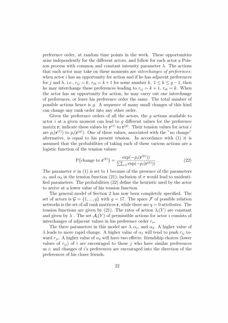
preference order, at random time points in the week. These opportunitiesarise independently for the different actors, and follow for each actor a Pois-son process with common and constant intensity parameter λ. The actionsthat each actor may take on these moments are interchanges of preferences :when actor i has an opportunity for action and if he has adjacent preferencesfor j and h, i.e., rij = k, rih = k + 1 for some number k, 1 ≤ k ≤ g− 1, thenhe may interchange these preferences leading to rij = k + 1, rih = k. Whenthe actor has an opportunity for action, he may carry out one interchangeof preferences, or leave his preference order the same. The total number ofpossible actions hence is g. A sequence of many small changes of this kindcan change any rank order into any other order.

Given the preference orders of all the actors, the g actions available toactor i at a given moment can lead to g different values for the preferencematrix r; indicate these values by r(1) to r(g). Their tension values for actor iare pi(r

(1)) to pi(r(g)). One of these values, associated with the ”no change”

alternative, is equal to his present tension. In accordance with (1) it isassumed that the probabilities of taking each of these various actions are alogistic function of the tension values:

P{change to r(k)} =exp(−pi(r

(k)))∑gh=1 exp(−pi(r(h)))

. (22)

The parameter σ in (1) is set to 1 because of the presence of the parametersα1 and α2 in the tension function (21); inclusion of σ would lead to unidenti-fied parameters. The probabilities (22) define the heuristic used by the actorto arrive at a lower value of his tension function.

The general model of Section 2 has now been completely specified. Theset of actors is G = {1, ..., g} with g = 17. The space F of possible relationnetworks is the set of all rank matrices r, while there are q = 0 attributes. Thetension functions are given by (21). The rates of action λi(Y ) are constantand given by λ . The set Ai(Y ) of permissible actions for actor i consists ofinterchanges of adjacent values in his preference order ri∗.

The three parameters in this model are λ, α1, and α2. A higher value ofλ leads to more rapid change. A higher value of α1 will tend to push rij to-ward rji. A higher value of α2 will have two effects: friendship choices (lowervalues of rij) of i are encouraged to those j who have similar preferencesas i; and changes of i’s preferences are encouraged into the direction of thepreferences of his closer friends.

22

The probabilistic model for friendship development in the fraternity isnow complete. Mathematically speaking, it is a continuous time Markovchain for the discrete matrix r. Special sub-models are:

• α1 = α2 = 0: purely random change;

• α2 = 0: change on the basis of reciprocity only.

The parameter λ cannot be set to 0, because that would imply that no changeoccurs at all. It is possible to consider the model where α1 = 0, α2 > 0, wherechanges occurs on the basis of balance only while reciprocity plays no role.This sub-model seems, however, very implausible theoretically, so we will notpay attention to this possibility.

4.2 Statistics for moment estimation

The first step to apply the estimation method of Section 3 is to choose statis-tics that capture the effects of the three parameters in the model. The effectsof the parameters were indicated above: λ determines rate of change, α1 reci-procity, and α2 balance. A statistic that is relevant for the amount of changefrom time t to time t + 1, is the sum of squared differences

‖ r(t + 1)− r(t) ‖2 =g∑

i,j=1i6=j

(rij(t + 1)− rij(t))2. (23)

Statistics that are relevant for the parameters α1 and α2 are the totals forreciprocity and balance over the set of all actors:

Rec(r(t + 1)) =2

g(g − 1)

∑1≤i<j≤g

(rij(t + 1)− rji(t + 1))2, (24)

Bal(r(t + 1)) =1

c

g∑i,j=1i6=j

φ(rij(t + 1))g∑

h=1h 6=i,j

(rih(t + 1)− rjh(t + 1))2,(25)

where c is a norming constant,

c = g(g − 2)g−1∑k=1

φ(k) .

23

The constants before the summation signs in (24) and (25) are such thatthese two statistics can be interpreted as mean squared differences of ranknumbers.

4.3 Null model: random change

The null model of random change (α1 = α2 = 0) is so simple, that someexplicit calculations can be performed without taking recourse to MonteCarlo simulation. The g vectors ri∗, i = 1, ..., g, are independent under thismodel, each following a continuous-time Markov process with λ expected in-terchanges of preferences per unit of time. Indicate the random number ofinterchanges in one time unit by L; then L has the Poisson distribution withparameter λ , and conditionally on L, the continuous-time Markov chain isequal to L steps of a discrete Markov chain. With some computations, it canbe concluded from the theory of discrete Markov chains that

E {g∑

j=1j 6=i

(rij(t + 1)− rij(t))2 | L} =

g−1∑i,j=1

(i− j)2(PL)ij ,

where P is the (g − 1)× (g − 1) transition matrix that applies to the singlenumbers rij. The elements of P are

p11 = pg−1,g−1 = 1− 1/g ,pii = 1− 2/g for i = 2, ..., g − 2 ,pi,i+1 = pi+1,i = 1/g for i = 1, ..., g − 2 ,pij = 0 for | i− j |≥ 2 .

It follows that

Eλ{g∑

j=1j 6=i

(rij(t + 1)− rij(t))2} =

∞∑h=0

g−1∑i,j=1

e−λλ−h

h!(i− j)2(P h)ij . (26)

The value of (26) can easily be computed numerically, and used for themoment estimation of λ from the outcome of ‖ r(t + 1)− r(t) ‖2.

These expressions can also be used to calculate the asymptotic value,which is also the upper bound, for (26). For λ → ∞, the asymptotic dis-tribution of ri∗(t + 1) is the uniform distribution over the space of all per-mutations of the numbers 1 to g − 1, irrespective of ri∗(t). Accordingly,

24

(P h)ij → 1/(g − 1) for h →∞, for all i, j. It follows that

limλ→∞

Eλ{g∑

j=1j 6=i

(rij(t + 1)− rij(t))2} =

1

g − 1

g−1∑i,j=1

(i− j)2 =g(g − 1)(g − 2)

6.

(27)Because this asymptotic value is known, we can replace the statistic‖ r(t + 1)− r(t) ‖2 by its normed value,

Dist(t, t + 1) =6

g2(g − 1)(g − 2)

g∑i,j=1i6=j

(rij(t + 1)− rij(t))2 .

Under the null model, 0 ≤ Eλ(Dist(t)) ≤ 1, and limλ→∞ Eλ(Dist(t)) = 1 .Figure 1 presents the graph of Eλ(Dist(t)).

=============================Insert Figure 1 here.=============================

The parameter λ was estimated separately for all weeks. This was doneusing the exact expected values (26), which led to moment estimates λ,and also using the Robbins-Monro procedure, yielding simulated momentestimates λRM. The results are presented in Table 1.

The differences λRM − λ are of the size of magnitude of less than 0.1standard error, in accordance with the N = 400 iterations used. This is acheck on the implementation of the simulation model and the Robbins Monromethod. The estimates of λ quickly decrease from λ = 177 at t = 1 to valuesaround 40 for t ≥ 5. This means that large changes in preferences occurredin the beginning, while the rate of change stabilized around week 5. Contraryto expectations, period 8, which due to the missing data for week 9 refers totwo weeks instead of one, does not yield a higher value for λ. To interpretthe numeric values of λ, note that λ is the expected number of interchangesof adjacent preferences per week.

25

Table 1. Null Model: Moment Estimatesand Robbins-Monro Moment Estimates

Period t Dist(t, t + 1) λ λRM S.E.(λRM )

1 0.3538 177.1 178.4 22.72 0.1934 84.7 84.4 11.43 0.1500 63.4 62.8 7.74 0.1597 68.1 67.4 8.15 0.1199 49.5 48.8 5.86 0.0872 34.9 34.6 4.37 0.0810 32.2 32.3 4.0

8-9 0.0960 38.7 39.0 4.010 0.1067 43.5 43.6 5.811 0.1123 46.0 45.8 6.312 0.1062 43.3 43.1 6.113 0.0787 31.3 30.8 4.214 0.0948 38.2 38.1 5.715 0.1012 41.0 40.6 4.7

The exact standard error of λ may be supposed to be an increasing func-tion of λ . This is only approximately the case for the estimates of Table 1.The deviations from strict increasingness are presumably a consequence ofdeviations between (8) and (15), due to the stochastic nature of the estima-tion by the Robbins Monro process.

4.4 Results for Models with Reciprocity and Balance

In this section we present estimation results for the model with only thereciprocity effect, and for the model with reciprocity as well as balance ef-fects. The interpretation of the numerical values of the estimated parametersα1 and α2 will be discussed in a following paper.

We first present results where the assumption of constant parameter val-ues over time is not made, and where separate estimates are obtained for eachperiod t = 1, ..., 15 , using moment estimation based on equation (3). Theestimates for the reciprocity model, where α2 = 0, are presented in Table 2.

26

Table 2. Reciprocity Model: Robbins-Monro Moment Estimates

Period t Dist(t, t + 1) Rec(t + 1) λ S.E.(λ ) α1 S.E.(α1 )

1 0.3538 26.43 178.2 27.7 0.0068 0.00372 0.1934 24.34 86.4 12.9 0.0094 0.00223 0.1500 25.88 66.2 9.0 0.0050 0.00384 0.1597 27.23 68.9 7.3 0.0052 0.00275 0.1199 29.69 49.8 6.2 0.0022 0.00326 0.0872 30.69 34.8 5.0 0.0030 0.00487 0.0810 26.68 31.0 3.7 0.0196 0.0048

8-9 0.0960 27.53 38.8 4.7 0.0054 0.003510 0.1067 28.28 44.5 6.4 0.0054 0.005011 0.1123 30.22 46.8 6.8 0.0025 0.003012 0.1062 29.51 44.0 6.8 0.0071 0.003113 0.0787 31.03 31.1 4.5 0.0012 0.004714 0.0948 29.84 38.2 5.3 0.0081 0.003915 0.1012 30.94 41.0 6.4 0.0036 0.0033

The estimates for λ are hardly different from those under the null model.The estimates for α1 are small, all positive, and quite variable. They exceedtwice their standard error in 4 out of 14 cases. This is more than expected bychance, but to have a good test of reciprocity, a more sensitive combinationprocedure is required than the mere count of the number of periods with asignificant parameter. This combination is given by the combined test (17)and yields tcomb = 6.03 . This indicates a strong significance of the reciprocityeffect. The average estimate α1 equals 0.0060 . Period 7 stands out in Table 2,the estimated reciprocity effect being considerably higher in this week. Thiscorresponds to the fact that the reciprocity tension function Rec(t) shows,during period 7, its greatest decrease Rec(8)−Rec(7) = −4.01 . Independentrepetitions of the estimation procedure did not lead to considerably differentresults, so this deviating result for period 7 cannot be attributed to a largerandom error, or non-convergence, in the Robbins Monro procedure. Furtheranalysis will have to reveal whether this effect is real or an artifact of themodel.

For the model with α1 as well as α2 as free parameters, the results arepresented in Table 3.

27

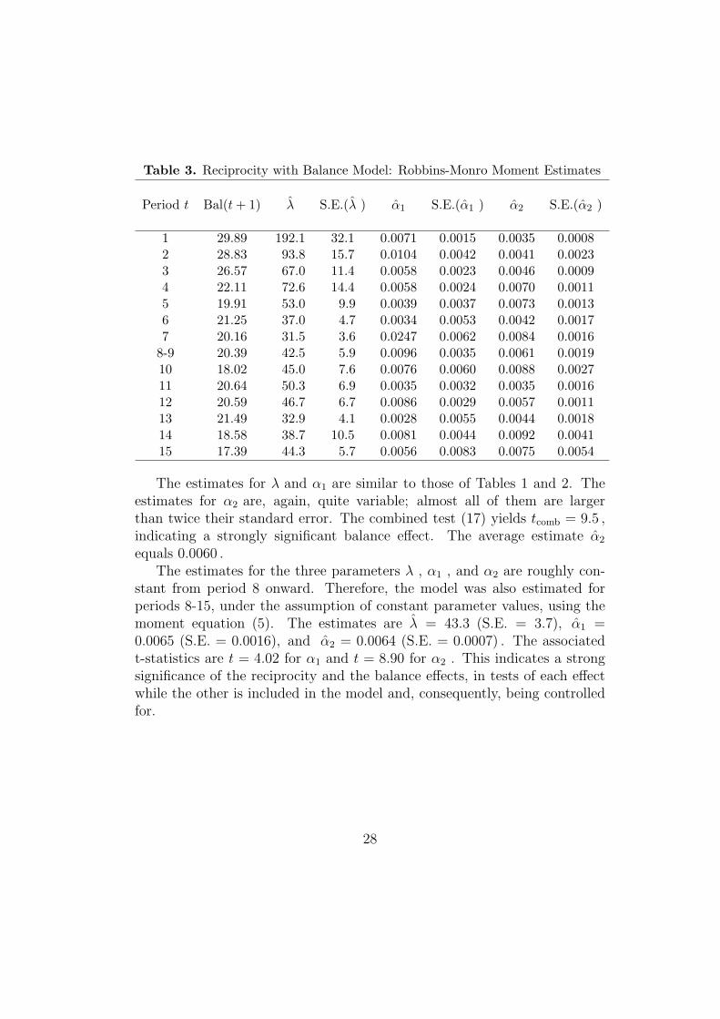
Table 3. Reciprocity with Balance Model: Robbins-Monro Moment Estimates

Period t Bal(t + 1) λ S.E.(λ ) α1 S.E.(α1 ) α2 S.E.(α2 )

1 29.89 192.1 32.1 0.0071 0.0015 0.0035 0.00082 28.83 93.8 15.7 0.0104 0.0042 0.0041 0.00233 26.57 67.0 11.4 0.0058 0.0023 0.0046 0.00094 22.11 72.6 14.4 0.0058 0.0024 0.0070 0.00115 19.91 53.0 9.9 0.0039 0.0037 0.0073 0.00136 21.25 37.0 4.7 0.0034 0.0053 0.0042 0.00177 20.16 31.5 3.6 0.0247 0.0062 0.0084 0.0016

8-9 20.39 42.5 5.9 0.0096 0.0035 0.0061 0.001910 18.02 45.0 7.6 0.0076 0.0060 0.0088 0.002711 20.64 50.3 6.9 0.0035 0.0032 0.0035 0.001612 20.59 46.7 6.7 0.0086 0.0029 0.0057 0.001113 21.49 32.9 4.1 0.0028 0.0055 0.0044 0.001814 18.58 38.7 10.5 0.0081 0.0044 0.0092 0.004115 17.39 44.3 5.7 0.0056 0.0083 0.0075 0.0054

The estimates for λ and α1 are similar to those of Tables 1 and 2. Theestimates for α2 are, again, quite variable; almost all of them are largerthan twice their standard error. The combined test (17) yields tcomb = 9.5 ,indicating a strongly significant balance effect. The average estimate α2

equals 0.0060 .The estimates for the three parameters λ , α1 , and α2 are roughly con-

stant from period 8 onward. Therefore, the model was also estimated forperiods 8-15, under the assumption of constant parameter values, using themoment equation (5). The estimates are λ = 43.3 (S.E. = 3.7), α1 =0.0065 (S.E. = 0.0016), and α2 = 0.0064 (S.E. = 0.0007) . The associatedt-statistics are t = 4.02 for α1 and t = 8.90 for α2 . This indicates a strongsignificance of the reciprocity and the balance effects, in tests of each effectwhile the other is included in the model and, consequently, being controlledfor.

28

5 Discussion

This paper has presented a statistical method to estimate parameters insimulation models from empirical data, and a rational-choice based approachto mathematical modeling of social network development.

Statistical estimation of parameters in simulation models is rare, presum-ably because simulation models often are regarded to be far removed fromempirical applications, and because the statistical machinery has been lack-ing. Hopefully, the presentation of some statistical machinery in this paperwill contribute to the mutual rapprochement between simulation models andempirical research. The estimation method based on the Robbins-Monromethod is quite computer-intensive. This may be a restriction to its useful-ness, but will be so to a decreasing extent. A disadvantage of the method isits lack of full statistical efficiency, due to the use of the method of moments;and the not quite satisfactory stability of the variance estimators (15). Moreresearch is needed on the judicious choice of statistics S as used in Section 3for the moment method, in view of the efficiency of the resulting estimators,and on more stable variance estimators. However, the use of precise, andtheoretically well-founded mathematical models can imply an efficiency gainthat makes up for this lack of statistical efficiency. More research is alsoneeded to derive measures of how well the model represents the data, and ofthe fit of the model.

The proposed class of models for social network development is based onindividually optimizing actors, bound by social, cognitive, and other con-straints. Due to the limitations of the part of Newcomb’s data set that isnow accessible, the main constraints represented in the model of Section 4 arethe current structure of the network and the simple (one could say: trivial)heuristic used by the actors to decrease their tension. Important constraintsfor Newcombe’s freshmen students such as the occupation and spatial lay-out of the rooms, as well as characteristics of the students (background,attitudes), were collected by Nordlie and Newcombe but seem to have beenlost.

Models of the type presented in Section 2 can be used in a statisticalanalysis of observational data on network evolution especially if importantconstraints are known in the data set. The model specification will have tobe based in part on theoretical modeling, in part on arbitrary or mathemat-ically convenient assumptions. Examples of the latter are the precise form

29

of the tension function (21), and of the probabilities (22) in Section 4. Thistheoretically arbitrary part of the model specification may be based, to someextent, on empirical results; for the rest, the results of the statistical analysisshould preferably be insensitive to this part of the model specification. Moreresearch is needed also on these points.

Our treatment of Newcomb’s fraternity data in this paper is not morethan an example of the proposed approach to modeling and estimation. Infuture work, we plan to have a more thorough look at the specification ofmathematical models for Newcomb’s data, and to apply our approach alsoto other empirical studies. An example is given by Van De Bunt, Van Duijn,and Snijders (1995).

References

[1] Bishop, Y.M.M., Fienberg, S.E., and Holland, P.W. (1975), Discretemultivariate analysis, Cambridge, MA: MIT Press.

[2] Borgatti, S., Everett, M.G., and Freeman, L.C. (1992), UCINET IVVersion 1.0 Reference Manual, Columbia: Analytic Technologies.

[3] Bowman, K.O., and Shenton, L.R. (1985), ”Method of moments”, p.467 – 473 in Encyclopedia of Statistical Sciences, vol. 5, S. Kotz, N.L.Johnson, and C. B. Read (eds.), New York: Wiley.

[4] Chow,G.C. (1983), Econometrics, Halliday Lithograph Corporation.

[5] Chung, K.L. (1967), Markov chains with stationary transition probabil-ities, New York: Springer Verlag.

[6] Doreian, P., Kapuscinski, R., Krackhardt, D., and Szczypula, J. (1994),”A brief history of balance through time”.

[7] Fararo, T.J., and Skvoretz, J. (1984), ”Biased networks and social struc-ture theorems: Part II”, Social Networks, 6, 223 – 258.

[8] Fararo, T.J. (1981), ”Biased networks and social structure theorems”,Social Networks, 3, 137 – 159.

30

[9] Fararo, T.J. (1989), The meaning of general theoretical sociology, Cam-bridge: Cambridge University Press.

[10] Fararo, T.J., and Hummon, N.P. (1994), ”Discrete event simulation andtheoretical models in sociology”, Advances in Group Processes, 11, 25 –66.

[11] Fararo, T.J., and Skvoretz, J. (1984), ”Biased networks and social struc-ture theorems: Part II”, Social Networks, 6, 223 – 258.

[12] Fienberg S.E., Meyer M.M. and Wasserman S. (1985), ”Statistical analy-sis of multiple sociometric relations”, Journal of the American StatisticalAssociation, 80, 51 – 67.

[13] Hoede, C. (1990), ”Social atoms: kinetics”, in Weesie, J., and Flap,H.D. (eds.), Social networks through time, p. 45-63, Utrecht: ISOR.

[14] Holland P. and Leinhardt S. (1975), ”Local structure in social net-works”, in Sociological Methodology - 1976, ed. D.R. Heise, San Fran-cisco: Jossey-Bass.

[15] Holland P. and Leinhardt S. (1977a), ”A dynamic model for social net-works”, Journal of Mathematical Sociology, 5, 5 – 20.

[16] Holland P. and Leinhardt S. (1981), ”An exponential family of probabil-ity distributions for directed graphs”, Journal of the American StatisticalAssociation, 76, 33 – 50.

[17] Karlin, S., and Taylor, H.M. (1975), A first course in stochastic pro-cesses, New York: Academic Press.

[18] Leenders, R.Th.A.J. (1994), ”Models for network dynamics: a Marko-vian framework”, submitted for publication.

[19] Maddala, G.S. (1983), Limited-dependent and qualitative variables ineconometrics, Cambridge: Cambridge University Press.

[20] Mayer, T.F. (1984), ”Parties and networks: stochastic models for rela-tionship networks ”, Journal of Mathematical Sociology, 10, 51 – 103.

31

[21] McFadden, D. (1973), ” Conditional logit analysis of qualitative choicebehavior”, in Frontiers in econometrics, P. Zarembka (ed.), New York:Academic Press.

[22] McFadden, D. (1989), ”A method of simulated moments for estimationof discrete response models without numerical integration”, Economet-rica, 57, 995 – 1026.

[23] Nevel’son, M.B., and Has’minskii, R.A. (1973), ”An adaptive Robbins-Monro procedure”, Automatic and Remote Control, 34, 1594 – 1607.

[24] Newcomb, T. (1961), The acquaintance process, New York: Holt, Rine-hart and Winston.

[25] Nordlie, P.G. (1958), A longitudinal study of interpersonal attraction ina natural group setting. Ph. D. Dissertation, University of Michigan.

[26] Pakes, A., and Pollard, D., ”The asymptotic distribution of simulationexperiments”, Econometrica, 57, 1027 – 1057.

[27] Pudney, S. (1989), Modelling individual choice, Oxford: Basil Blackwell.

[28] Robbins, H., and Monro, S. (1951), ”A stochastic approximationmethod”, Annals of Mathematical Statistics, 22, 400 – 407.

[29] Rapoport, A. (1951), ”Nets with distance bias”, Bulletin of mathemat-ical biophysics, 13, 85 – 91.

[30] Rapoport, A. (1957), ”Contribution to the theory of random and biasednets”, Bulletin of mathematical biology, 19, 257 – 277.

[31] Ruppert, D. (1991), ”Stochastic approximation”, in Handbook of Se-quential Analysis, eds. B.K. Gosh and P.K. Sen, New York: MarcelDekker.

[32] Skvoretz, J. (1991), ”Theoretical and methodological models of networksand relations”, Social Networks, 13, 275 – 300.

[33] Snijders, T.A.B. (1991), ”Enumeration and simulation methods for 0-1matrices with given marginals”, Psychometrika, 56, 397 – 417.

32

[34] Snijders, T.A.B., Van Dam, M.J.E.M., and Weesie, J. (1994), ”Whocontributes to public goods? With an application to local economicpolicies in The Netherlands”. Journal of Mathematical Sociology, 19,149 – 164.

[35] Stokman, F.N., and Zeggelink, E.P.H. (1993), ”A dynamic access modelin policy networks”, Groningen: ICS.

[36] Van De Bunt, G.G., Van Duijn, M.A.J., and Snijders, T.A.B. (1995),”Friendship networks and rational choice”, International Social NetworkConference, London, 6-10 July, 1995.

[37] Venter, J.H. (1967), ”An extension of the Robbins-Monro procedure”,Annals of Mathematical Statistics, 38, 181 – 190.

[38] Wasserman, S. (1977), Stochastic models for directed graphs, Ph.D. dis-sertation, University of Harvard, Dept. of Statistics.

[39] Wasserman, S. (1979), ”A stochastic model for directed graphs withtranstion rates determined by reciprocity”, in Sociological Methodology1980, K.F. Schuessler (ed.), San Francisco: Jossey-Bass.

[40] Wasserman, S. (1980), ”Analyzing social networks as stochastic pro-cesses”, Journal of the American Statistical Association, 75, 280 – 294.

[41] Wasserman, S., and Faust, K. (1994), Social Network Analysis: Meth-ods and Applications, New York and Cambridge: Cambridge UniversityPress.

[42] Zeggelink, E.P.H. (1993), Strangers into Friends: The evolution offriendship networks using an individual oriented modeling approach,Amsterdam: Thesis Publishers.

[43] Zeggelink, E.P.H. (1994), ”Dynamics of structure: an object-orientedapproach”, Social Networks, 16,

[44] Zeggelink, E.P.H. (1995), ”Group formation and the emergence of soli-darity in friendship networks”, Journal of Mathematical Sociology.

33