statistics of vix futures and applications to trading
TRANSCRIPT

Statistics of VIX Futures and Applications to Trading
Exchange-Traded Products
M. Avellaneda∗ and A. Papanicolaou†
August 29, 2017
Abstract
We study the dynamics of VIX futures and ETNs/ETFs. We find that contrary to classical
commodities, VIX and VIX futures exhibit large volatility and skewness, consistently with the
absence cash-and-carry arbitrage. The constant-maturity futures (CMF) term-structure can
be modeled as a stationary stochastic process in which the most likely state is a contango
with V IX ≈ 12% and a long-term futures price V∞ ≈ 20%. We analyse the behavior of
ETFs and ETNs based on constant-maturity rolling futures strategies, such as VXX, XIV,
VXZ, assuming stationarity and through a multi-factor model calibrated to historical data.
We find that buy-and-hold strategies consisting of shorting ETNs which roll long futures or
buying ETNs which roll short futures produce theoretically sure profits assuming that CMFs
are stationary and ergodic. To quantify further, we estimate a 2-factor lognormal model with
mean-reverting factors to VIX and CMF historical data from 2011 to 2016. The results confirm
the profitability of buy-and-hold strategies, but also indicate that the latter have modest Sharpe
ratios, of the order of SR = 0.5 or less, and high variability over 1-year horizon simulations.
This is due to the surges in VIX and CMF backwardations which are experienced sporadically,
but also inevitably, in the volatility futures market.
∗Courant Institute of Mathematical Sciences, New York University, 251 Mercer Street, New York, N.Y. [email protected]†Department of Finance and Risk Engineering, NYU Tandon School of Engineering, 6 MetroTech Center, Brook-
lyn, NY 11201 [email protected]
1

Contents
1 The Volatility Index: stylized facts 3
2 VIX Futures 5
2.1 Principal Component Analysis . . . . . . . . . . . . . . . . . . . . . . . . . . . . . . 6
3 Rolling Futures and Exchange-Traded Notes 9
3.1 Rolling the front-month contract . . . . . . . . . . . . . . . . . . . . . . . . . . . . . 9
3.2 Continuous (daily) rolling . . . . . . . . . . . . . . . . . . . . . . . . . . . . . . . . . 14
3.3 Exchange-traded funds and notes . . . . . . . . . . . . . . . . . . . . . . . . . . . . . 15
3.4 Integrated TRI equations and ETP buy-and-hold strategies . . . . . . . . . . . . . . 18
3.5 Long-time behavior of ETNs under stationarity . . . . . . . . . . . . . . . . . . . . . 19
4 A Parametric Model for CMFs 20
4.1 Lognormal Markov model for VIX . . . . . . . . . . . . . . . . . . . . . . . . . . . . 20
4.2 From VIX to CMFs . . . . . . . . . . . . . . . . . . . . . . . . . . . . . . . . . . . . 21
4.3 Profitability of rolling futures strategies . . . . . . . . . . . . . . . . . . . . . . . . . 23
5 Parameter Estimation 24
5.1 Filtering and parameter estimation . . . . . . . . . . . . . . . . . . . . . . . . . . . . 25
5.2 Qualitative analysis of parameter estimates . . . . . . . . . . . . . . . . . . . . . . . 29
6 Application of 2-Factor OU Model to ETNs 31
6.1 Dynamics of ETNs . . . . . . . . . . . . . . . . . . . . . . . . . . . . . . . . . . . . . 31
6.2 Simulated one-month ETN (VXX) . . . . . . . . . . . . . . . . . . . . . . . . . . . . 33
6.3 Simulated five-month basket ETN (VXZ) . . . . . . . . . . . . . . . . . . . . . . . . 35
6.4 Simulated one-month inverse ETN (XIV) . . . . . . . . . . . . . . . . . . . . . . . . 36
7 Conclusion 37
2
1 The Volatility Index: stylized facts
Volatility futures and exchange-traded products (ETPs) are broadly traded instruments in today’s
markets. VIX-related exchange-traded funds (ETFs) and exchange-traded notes (ETNs), launched
in early 2009, experienced exponential growth in trading volumes. There appears to be a strong
appetite by institutional investors for volatility products, for the purpose of managing tail-risk and
hedging, as well trading S&P500 option implied volatility as a stand-alone asset class. 1
The Chicago Board Options Exchange Volatility index, VIX, ([CBOE]) is equal, at any given
time, to the square-root of the value of a basket of short-term S&P500 options, in which the portfolio
weights depend on the moneyness and time-to-maturity of each constituent option. The portfolio’s
value corresponds to the fixed leg in a 30-day variance swap on the S&P 500 Index (for details, see
e.g., [Whaley1993], [CBOE]). In 2006, the CBOE launched VIX futures contracts which settle on
the spot VIX and provide a means of trading volatility as a commodity.
There is no well-accepted way to “carry” or to “store” VIX for delivery against a futures contract,
as one may attempt to do with index or commodity futures. The main reason for this is that
the weights of the VIX basket are not known before the settlement date. Therefore, “carrying”
VIX would imply dynamic trading (“rolling”) at-the-money-forward and near-the-money, constant
maturity, 30-day options. The cost of such strategies cannot be calculated accurately in advance.2
In the event of a sudden market shock, or the perception of an impending shock, the demand for S&P
500 puts, is met by option sellers which will raise option-implied volatilities. The lack of “storage”
also implies that, once the equity market’s demand for protection subsides, implied volatilities will
drop likewise. The conclusion is that VIX should be much more volatile than commodities such as
crude oil or equity indexes. 3
The top left plot of Figure 1 displays the VIX time series from 2004 through 2016. Noticeable
1A similar exchange-traded volatility market exists in Europe around the V STOXX index, which tracks theshort-term implied volatility of STOXX50, in Deutsche-Borse-XETRA.
2An additional complication for replicating VIX with options stems from the fact that VIX is defined as thesquare-root of the value of the basket, but we shall not discuss this further.
3Certain commodities, such as electricity or natural gas, are technically difficult to distribute and store. Probablyfor these reasons they give rise to VIX-like price spikes. On the other hand, crude oil, for example, benefits fromample storage and transportation infrastructures, so that its price volatility is primarily linked to major changes inproduction/delivery.
3

spikes in the time series are see in October 2008 (Lehman Brothers collapse), June 2010 (Greek
debt crisis), August 2011 (U.S downgrade by Standard and Poor’s), and August 2015 (Reminbi
devaluation).
We find, empirically, that the time-series of VIX behaves like a stationary process. This state-
ment can be justified statistically, to some extent, using VIX end-of-day historical values for the
index. If we use the period from January 1 1990 to May 31, 2017 (6906 daily observations), Matlab’s
version of the Augmented Dickey-Fuller test (adftest) rejects the presence of a unit root, returning
a DFstat=-3.0357 with critical value CV= -1.9416 and pvalue=0.0031. We point out, however, that
adftest does not reject unit-roots over other time windows, particularly if the events of 2008 are
removed from the data. We also studied the stationarity of VIX by a different method, which does
not involve the parametric assumptions made in Dickey-Fuller by splitting the VIX time series into
two samples and performing a 2-sample Kolmogorov-Smirnoff (KS) test on the daily differences in
VIX. Figure 1 shows the results of the KS tests, which support stationarity, the histogram of VIX,
and a power-law fit to the right-tail distribution. The empirical mean is 19.1, the mode is 11.98,
and the right-tail can is fitted to a Pareto tail with exponent α = −3.4. This shows that, as a
random variable, VIX is definitely skewed to the right with a heavy tail. On the other hand, VIX
has never closed below 9 as of this writing. Once again, we find that we cannot reject a unit root
if the 2008 crisis is included in the portion of data before the split. Thus, statistically speaking, we
may accept stationarity of VIX if we include the 2008 period in the sample, but we also find that
tests conducted over smaller time windows may not be conclusive.
Taking into account the well-known theory of volatility risk-premium, [CW09], we expect that
typically long-dated futures trade higher than the long-term average of VIX. On the other hand,
the most likely level of the VIX empirical distribution is significantly lower than the average. This
is consistent with the fact the futures term-structure is typically upward-sloping, or in contango.
The presence of heavy tails for the VIX distribution also indicates also that, sporadically, spot
VIX will be higher than its long-term average, so there are periods of backwardation of the futures
curve, either partly (only for front-month contracts) or fully, across the entire term-structure. These
periods of backwardation can be seen as VIX surges rapidly, driven by exogenous news and the
4

0
20
40
60
80
100VIX Daily Closing (1/2/2004 to 1/3/2017)
02−Ja
n−2004
30−D
ec−
2004
27−D
ec−
2005
22−D
ec−
2006
21−D
ec−
2007
18−D
ec−
2008
16−D
ec−
2009
14−D
ec−
2010
09−D
ec−
2011
10−D
ec−
2012
06−D
ec−
2013
04−D
ec−
2014
02−D
ec−
2015
29−N
ov−
2016
0
20
40
60
80
100KS Test for Split Samples
VIX
Level
02−Ja
n−2004
30−D
ec−
2004
27−D
ec−
2005
22−D
ec−
2006
21−D
ec−
2007
18−D
ec−
2008
16−D
ec−
2009
14−D
ec−
2010
09−D
ec−
2011
10−D
ec−
2012
06−D
ec−
2013
04−D
ec−
2014
02−D
ec−
2015
29−N
ov−
20160 500 1000 1500 2000 2500 3000 3500
0
0.2
0.4
0.6
0.8
1
KS
Reje
ct
0 10 20 30 40 50 60 70 80 900
50
100
150
200
250
300
350
Empirical VIX Distribution (1/2/2004 to 1/3/2017)
20 30 40 50 60 70 8010
−3
10−2
10−1
100
Fitted VIX Peaks over 25%
data
Fitted Pareto
Figure 1: Top Left: The time series of VIX, from 2004 through 2016. Top Right: Two-sample
Kolmogorov-Smirnoff (KS) test for the daily changes of VIX, with different splitting dates in the data.
If the 2008 crisis is included in the left data sample, then KS does not reject. Bottom Left: Empirical
distribution from VIX time series. Mean=19.1 and mode=11.98. Bottom Right: Fit of a Pareto density
p(v) = c(v− v0)a to the empirical distribution of VIX values over 25 (vertical axis in log scale). Estimated
parameters are v0 = 5, a = −3.4, and c = 8.8132.
increase in short-term option premia.
2 VIX Futures
Currently, VIX futures have 9 open monthly expirations as well as six additional contracts settling
weekly in the front of the curve4. VIX futures provide a straightforward approach for market
participants to position in 30-day forward near-the-money volatility corresponding to each of the
4 This article will concern the monthly contracts, where the bulk of the liquidity is concentrated.
5

settlement dates. 5
To capture the evolution of the VIX futures term-structure, it is convenient to work with
constant-maturity futures (CMFs).6 Accordingly, we define V τt as the price of a theoretical fu-
tures contract with maturity (or tenor) τ observed at date t. In practice, V τt is defined as a linear
interpolation between the two successive monthly contracts which expire immediately before and
immediately after τ years, i.e. such that their maturities “bracket” τ . If τ is shorter than the
maturity of the first monthly futures, V τ is defined as the linear interpolation between spot VIX
and the price of the first contract. Denoting by F1 and F2 the prices of the monthly contracts (or
VIX and the first contract) which have maturities τ1 and τ2, τ1 ≤ τ < τ2, we have
V τ =τ2 − ττ2 − τ1
F1 +τ − τ1τ2 − τ1
F2 . (1)
If F1 = VIX then τ1 = 0.7 With this approach, we can build the constant-maturity futures curve
from the available date on each trading date and perform statistical analysis on the data using daily
observations of the curves.
Our main modeling assumption is that the time-series of CMFs is stationary: i.e. for each τ the
time series V τt , 0 < t <∞ can be modeled as stationary process.
2.1 Principal Component Analysis
We considered the time series of daily settlement prices from February 8, 2011 to December 15,
2016 for the 9 open monthly VIX futures contracts, which have ticker symbols VX1, VX2, VX3,....,
VX9, as well as the (spot) VIX end-of-day value corresponding to each date. We discard the 9th
monthly contract, after we found that VX9 is not liquid and that the settlement prices tend to be
noisy and often missing. This leaves us with data on VIX and the first 8 monthly contracts. From
5VIX futures settle in the morning of the Wednesday of the week of the third Friday of the corresponding settlementmonth.
6This is entirely similar to the concept of Constant Maturity Treasuries [H.15], see also [CK13] who first studiedit for VIX futures.
7Clearly, linear interpolation is a possible choice but by no means the only one. Linear interpolation shall bereplaced by a smooth function of τ later on, when we introduce a parametric model for the term-structure, but thereis little difference in practice, except for the somewhat annoying fact that the derivative with respect to τ has jumpsin the linear interpolation model.
6
this data, we constructed 8 CMFs using the linear weights as in (1), corresponding to the maturities
τj = j 30365 with j = 0, 1, 2 . . . , 7, spanning from VIX (τ = 0 to 8 months. There are N = 1, 499
observed dates.
We considered the N × 8 data matrix
Vij = ln(Vτjti )− ln(V τj ) , i = 1, . . . N, j = 0, . . . 7,
where
ln(V τj ) =1
N
N∑i=1
ln(Vτjti ) .
We performed a singular-value decomposition of the data matrix. The singular value decomposition
(SVD) decomposes the centered matrix,
V = USψ′ ,
where U is an N × 8 orthonormal matrix, S is an 8 × 8 diagonal matrix containing the singular
values, and ψ is an 8× 8 orthonormal matrix whose columns are the principal components used to
form any given futures curve. In other words, we have
ln(Vτjti ) = ln(V τj ) +
8∑`=1
ai`ψj` ,
where the coefficient matrix is a = US. Figure 2 shows the results of the PCA.
We note that this analysis differs from [CK13], where the authors used PCA to analyze 1-day
log-returns; see also [LS], [Laloux et al.], and [Dobi]. In contrast, we consider here the fluctua-
tions of the VIX futures curve around its long-term average. This is consistent with the mean-
reversion/stationarity assumption, and the ansatz described above. In other words, this approach
to PCA is intended to determine various curves which are needed to ‘reconstruct” the CMF curve
at any particular date, viewed as a superposition of shapes. We call this the Equilibrium PCA, to
distinguish it from the analysis [CK13]. Equilibrium PCA provides an identikit of the VX curve,
7

in the spirit of image recognition: each component is seen as providing a “shape” or feature which
is superimposed to the average, with a corresponding loading coefficient. Each curve in the data
would correspond to a set of loadings applied to the different principal components.
We found that the first principal component accounts for 72% of the term-structure shape,
adding the second component increases it to 90%, adding the third increases it to 96%, and fourth
increases it to 97%. In addition, Figures 3 and 4 show poor quality for selected dates of fit when
having only one component and a significant improvement from inclusion of a second. Hence, it is
reasonable to consider a parsimonious model with d = 2:
ln(Vτjti ) = ln(V τj ) +
2∑`=1
ai`ψj` + εi ,
where εi is a noise term.
Using the Equilibrium PCA we determine the most likely CMF curve given the data. To find it,
we consider the time series of the loadings on the different shape factors ai`, i = 1, 2, ..., N for each
` and calculate the mode, or most frequently observed value, for each `. Assuming independence
(or weak dependence) between the factors, we postulate that the most likely CMF curve is
mode(ln(Vti)
)≈ ln(V ) +mode
(ai1
)ψ1 +mode
(ai2
)ψ2 .
The top plots in Figure 5 show the histograms of ai1 and ai2, and the bottom plot shows the
most-likely curve, which is clearly a contango.
8

1 2 3 4 5 6 7 810
-2
10-1
100
101
102
Principle components of Futures Curves
τ (in months)1 2 3 4 5 6 7 8
-0.8
-0.6
-0.4
-0.2
0
0.2
0.4
0.6
0.8Component Vectors
component 1component 2component 3component 4
Figure 2: Left: For the CMFs, the singular values from the SVD’s diagonal matrix S shown on log scale.
The first singular component alone accounts for 72% of variation, adding the second component increases it
to 90%, adding the third increases it to 96%, and fourth increases it to 97%. Right: The first four singular
vectors; the “zero-th”-order component is just the overall average level ln(V τ ) = 1N
∑i ln(V τti ).
3 Rolling Futures and Exchange-Traded Notes
In a typical rolling futures strategy, positions are transferred from one expiration to another as
contracts expire. Perhaps the simplest example is investing in a long position in the first contract,
reinvesting all profit/losses in futures and, on the expiration date of the contract, close the long
position and simultaneously open a long position for the same dollar amount in the second contract8
3.1 Rolling the front-month contract
We denote the futures contract maturing at date T1 by Ft,T1, where t is the current date. We
consider the situation of a fund that buys a number of contracts with notional value equal to the
equity in the fund, rebalances daily investing the profit/loss in futures, and rolls the entire position
into the next contract at the expiration date of the current contract9. We assume that the cash in
the fund is remunerated at rate r and neglect futures margin costs and other expenses. The total
8VIX futures settle in the morning of the contract’s expiration date. If we use daily close-to-close data it somewhatsimpler, to roll the position at the close of the day prior to the futures’ expiration date. One could also let the firstcontract expire and open simultaneously a position in the second contract. However, the latter strategy would requireintraday data for backtesting purposes. We also reinvest profits, which is consistent with the way ETN indexes areconstructed.
9Rebalancing is not necessary, but it is consistent with how an ETP operates: the notional amount invested infutures is equal to the total equity of the fund at any given time.
9

0 1 2 3 4 5 6 712
13
14
15
16
17
18
VX Curve Reconstructed with 1 Components
0 1 2 3 4 5 6 712
13
14
15
16
17
18
VX Curve Reconstructed with 2 Components
Maturity (in months)0 1 2 3 4 5 6 7
12
13
14
15
16
17
18VX Curve Reconstructed with 3 Components
Maturity (in months)0 1 2 3 4 5 6 7
12
13
14
15
16
17
18VX Curve Reconstructed with 4 Components
Figure 3: PCA reconstruction of VX futures curve for April 10th 2014. PCA calculated from daily VX
curves from February 8th 2011 to December 15th 2016.
10
0 1 2 3 4 5 6 725
30
35
40
45
50
VX Curve Reconstructed with 1 Components
0 1 2 3 4 5 6 725
30
35
40
45
50
VX Curve Reconstructed with 2 Components
Maturity (in months)0 1 2 3 4 5 6 7
25
30
35
40
45
50VX Curve Reconstructed with 3 Components
Maturity (in months)0 1 2 3 4 5 6 7
25
30
35
40
45
50VX Curve Reconstructed with 4 Components
Figure 4: PCA reconstruction of VX futures curve for August 8th 2011. These curves are not those of the
VIX’s most-likely state, but rather a tumultuous period around the first-ever downgrade of U.S. government
debt.
11

-0.05 0 0.05 0.10
20
40
60
80
100
120
Histogram of 1st PCA Weight
-0.15 -0.1 -0.05 0 0.05 0.10
20
40
60
80
100
120
140
Histogram of 2nd PCA Weight
Maturity (in months)0 1 2 3 4 5 6 7
13
14
15
16
17
18
19
20
21
22Most Likely Curve
most likely curvemean curve
Figure 5: Top Plots: The histogram of weights for the 1st and 2nd principal components, ai1 and ai2
respectively. Bottom Plot: Recall mean VIX higher than mode VIX. Here mean curve is higher than
mode curve, mode(ln(Vti)
)≈ ln(V ) +mode
(ai1)ψ1 +mode
(ai2)ψ2.
12

value of the fund, It, satisfies
dItIt
=
dFt,T1Ft,T1
+ rdt if t < T2 − dt
dFt,T2Ft,T2
+ rdt if t ≥ T2 − dt ,
(see Chapter 7 in [Ber16]). Here, T1 is the expiration date of the front contract, T2 is the expiration
date of the second contract, r is the interest rate, and dXt = Xt+dt − Xdt is the one-day change
from date t to t+ dt. We shall refer to It as the total return index or TRI of the strategy.
It is convenient to define the function
φ(t) =
Ft,T1
if t < T2 − dt
Ft,T2if t = T2 − dt ,
(2)
which represents the settlement price of the front-month contract at time t. Writing
φ(t) = b(t)Ft,T1+ (1− b(t))Ft,T2
, (3)
where b(t) = 1 if t < T2 and b(T ) = 0 if t = T2, we have
dφ(t) = b(t)dFt,1 + (1− b(t))dFt,T2 + (Ft,T2 − Ft,T1)δ(t− T2)dt ,
where δ(·) is the Dirac delta. Therefore, from equation (2) we have
dφ(t)
φ(t)=dItIt− rdt+
(Ft,T2− Ft,T1
)
φ(t)δ(t− T2)dt ,
or
dItIt
=dφ(t)
φ(t)− (Ft,T2 − Ft,T1)
φ(t)δ(t− T2)dt+ rdt .
Suppose that the front-month contract price follows a stationary distribution. Then, heuristically,
13
if the curve is in contango, rolling a long position will lose money on average and, conversely it will
earn money when the curve is in backwardation10. Similar considerations apply to other rolling
strategies. For instance, one could envision a strategy which rolls the futures in the middle of the
month, i.e. when θ + t = T1+T2
2 .11
3.2 Continuous (daily) rolling
Consider a yet-to-be-determined, decreasing function b(t) such that b(T1+) = 1 and b(T2) = 0,
where b(t) represents the fraction of the total number of contracts invested in the front contract,
and 1− b(t) is the fraction invested in the second-month contract. The (contract-weighted) average
maturity is therefore
θ(t) = b(t)(T1 − t) + (1− b(t))(T2 − t) .
If we set θ(t) = θ = constant , we find that b(t) = T−t−θT2−T1
and b(t) = − 1T2−T1
. According to the
definition of CMF futures given above, we have
φ(t) = b(t)Ft,T1 + (1− b(t))Ft,T2 = V θt ,
whence
dV θt = b(t) dFt,T1+ (1− b(t)) Ft,T2
+ (Ft,T2− Ft,T1
)dt
T2 − T1.
In particular, setting
w1(t) =b(t)Ft,T1
V θt, w2(t) =
(1− b(t))Ft,T2
V θt,
10This is clear if the processes are discrete or have finite variation. The assertion is also correct in the case ofcontinuous-time diffusions, as we show hereafter
11Mid-month rolling is essentially the strategy used by the US Oil ETN, USO.
14
we obtain
dV θtV θt
= w1(t)dFt,T1
Ft,T1
+ w2(t)dFt,T2
Ft,T2
+Ft,T2
− Ft,T1
V θt
dt
T2 − T
= w1(t)dFt,T1
Ft,T1
+ w2(t)dFt,T2
Ft,T2
+[∂ln(V τt )
∂τ
]τ=θ
dt .
(4)
It follows that the TRI of a continuous rolling long futures strategy with average constant maturity
θ satisfies
dIθtIθt
= w1(t)dFt,T1
Ft,T1
+ w2(t)dFt,T2
Ft,T2
+ rdt
=dV θtV θt−[∂ln(V τt )
∂τ
]τ=θ
dt+ rdt . (5)
The daily return of the index is the sum of the daily percent change of the CMF with maturity θ
and a “drift” term which depends on the slope of the CMF curve at τ = θ. This term is negative if
the curve is in contango and positive if the curve is in backwardation at τ = θ. The weights w1(t)
and w2(t) correspond to the proportions of assets (dollar-weights) invested in each of the contracts
in order to maintain a constant maturity θ.12.
3.3 Exchange-traded funds and notes
Most, but not all, VIX ETFs and ETNs correspond to constant-maturity rolling strategies13. For
θ = 30 days, the above example corresponds to the investable index tracked by VXX, the most
liquid VIX ETN. Inverse VIX ETNs and ETFs, such as XIV and SVXY correspond to rolling short
12Because contract prices are typically different, the weights depend on the futures prices as well as on the times-to-maturity of each contract.
13For information about VIX ETNs, see [CK13] and [ETNs]
15
positions, i.e., have total-return indexes
dJθtJθt
= −w1(t)dFt,T1
Ft,T1
−−w2(t)dFt,T2
Ft,T2
+ rdt
= −dVθt
V θt+[∂ln(V τt )
∂τ
]τ=θ
dt+ rdt . (6)
In the latter case, the exposure to contango is positive: the strategy value has a positive drift if the
CMF curve is in contango. Leveraged ETFs, such as UV XY associated with long or short front
month continuous rolling are defined similarly.
Another noteworthy example of a VIX ETN which is not a simple rolling futures strategy, is
the VXZ, which is constructed using 4 rolling contracts VX4, VX5, VX6 and VX7. It corresponds
to the phi-function
φ2(t) =b(t)
3Ft,T4
+1
3Ft,T5
+1
3Ft,T6
+1− b(t)
3Ft,T7
,
where b(t) drops linearly from 1 to zero between T3 and T4. The corresponding total-return index
is defined by
dIV XZ
IV XZt
=dφ2(t)
φ2(t)− 1
3φ2(t)
3∑i=1
(Ft,T4+i− Ft,T3+i
T4+i − T3+i
)dt+ rdt
=dφ2(t)
φ2(t)− 1
3φ2(t)
3∑i=1
V θit
[∂lnV τt∂τ
]τ=θi
dt+ rdt ,
where θi = 90 + 30× i days. Notice that can we can also view φ2(t) as the average of three CMFs,
namely
φ2(t) =1
3
(V θ1t + V θ2t + V θ3t
).
The average maturity of VXZ is θ1+θ2+θ33 = (120 + 150 + 180)/3 = 150 days, i.e. 5 months. Table
1 lists some of the VIX ETNs commonly traded in 2017.
16

ETN leverage average maturity (months) inception date
VXX 1 1m Jan 2009VXZ 1 5m Jan 2009XIV -1 1m Nov 2010
UVXY 2 1m Oct 2011ZIV -1 5m Nov 2010
TVIZ 2 5m Nov 2010
Table 1: Some of the VIX ETNs with high trading volume in 2017.
2010 2011 2012 2013 2014 2015 2016 20170
5000
10000
VXX and VXZ Daily Closing (3/1/2010 to 3/1/2017)
0
200
400
VXX
VXZ
Figure 6: The historical time series of VXX and VXZ prices. The VXX rolls between VX1 and VX2 to
maintain a 1-month average maturity, and the VXZ rolls between the VX4, VX5, VX6 and VX7 contracts
to maintain an average maturity of 5-months. The VXZ has less volatility than the VXX because it is an
average and because it rolls in longer-term contracts; the VXX rolls in 1 and 2-month contracts that are
typically more volatile.
17
3.4 Integrated TRI equations and ETP buy-and-hold strategies
Next, we derive integrated form of the equations (5) and (6). By Ito’s Formula, we have
d lnV τt =dV τtV τt− 1
2
(dV τtV τt
)2
, (7)
where the last term on the right-hand side corresponds to the quadratic variation process of lnV τt .
A similar equation holds for lnIτt . From equation (5) we also deduce that the quadratic variations
of both processes are equal:
(dV τtV τt
)2
=(dIτtIτt
)2
.
Thus, equation (5) is equivalent to
d lnIτt = d lnV τt −∂lnV τt∂τ
dt+ rdt ,
or, in integrated form,
IτtIτ0
= ertV τtV τ0
exp(−
t∫0
∂lnV τs∂τ
ds). (8)
In a similar vein, consider an inverse ETN which tracks a CMF with maturity θ. If we denote
this ETN (or its underlying index) by Jθ, we have, from (6),
JτtJτ0
= ertV τ0V τt
exp( t∫
0
∂lnV τs∂τ
ds). (9)
Equations (8) and (9) display an explicit relation between the total-return indexes of ETNs for
rolling futures, the constant-maturity futures and the slope of the CMF curve. The derivation of
the equations for total-return index of VXZ, as well as other ETNs based on rolling a basket of
futures, is left to the reader.
18
3.5 Long-time behavior of ETNs under stationarity
As an application, consider a trader who sells short an ETN tracking Iτ and invests the proceeds
in a money market account paying interest r. The market value of his portfolio at time t in dollars
at time zero is ,
Iτ0 − e−rtIτt = Iτ0
(1− V τt
V τ0exp(−
t∫0
∂lnV τs∂τ
ds))
.
Similarly, a trader who borrows Jτ0 dollars and invests in the inverse ETN with maturity τ will
have a present value equal to
e−rt Jτt − Jτ0 = Jτ0
(V τ0V τt
exp( t∫
0
∂lnV τs∂τ
ds)− 1
),
suggesting that the trader will achieve unbounded gains by investing in the inverse VIX ETN in
the long run.
If we assume that V τt is ergodic (a mild assumption in this context) then
limt→∞
1
t
t∫0
∂lnV τs∂τ
ds = E[∂lnV τ
∂τ
],
where the expectation is taken over the equilibrium measure of the CMF curve process. We conclude
that:
Proposition: Assume that V τt is a stationary and ergodic process and that E[∂lnV τ
∂τ
]> 0. Then,
limt→∞
(Iτ0 − e−rtIτt
)= 0 and
limt→∞
(e−rtJτt − Jτ0
)= ∞ . (10)
In other words, under our assumptions, shorting the long VIX ETN and going long the short VIX
ETN both produce sure profits as t→∞.
Clearly, these theoretical profits are not free of risk. Equations (8) and (9) show that if V τt is
volatile, the random variableV τ0V τt
can be very small even if t is large. Backwardation associated
19

with high volatility could make∂lnV τs∂τ negative as well. Hence the return of the buy-and-hold, long
XIV, could be negative over any time interval [0, t].
In order to quantify the profitability, if any, of such strategies in the real world, we resort to a
simple parametric model for the evolution of CMFs. This model shall provide further insight on
whether of not we can regards CMFs as being a stationary process and on the performance rolling
futures strategies and trading ETPs.
4 A Parametric Model for CMFs
4.1 Lognormal Markov model for VIX
We consider a model in which log(V IXt) follows a multi-factor Gaussian diffusion, i.e.
V IXt = exp( d∑i=1
Xit
),
with each factor Xi following a one-dimensional Ornstein-Uhlenbeck (OU) process
dXit = κi (µi −Xit) dt+ σidWPit , κi > 0, i = 1, ..., d .
Here (WP1t , ...W
Pd t) is a d-dimensional vector of Brownian motions with correlation matrix ρij .
According to this model, V IX is stationary with an equilibrium distribution such that VIX is
log-normal, with
E[lnV IX] =
d∑i=1
µi , var(lnV IX) =
d∑ij=1
σiσjρijκi + κj
,
and, accordingly,
E[V IX] = exp( d∑i=1
µi +1
2
d∑ij=1
σiσjρijκi + κj
).
20

4.2 From VIX to CMFs
To extend this model to CMFs, we assume (see e.g. Cox, Ingersoll, Ross [CIR1985]) that there
exists a probability measure Q and a WP -adapted d-dimensional process λt (the market prices of
risk or MPRs) such that (i) the processes
dWQit := dWP
it + λitdt i = 1, ..., d ,
are standard Brownian motions under Q (with correlation ρij), and (ii) every futures price is the
expected value under Q of VIX at the corresponding expiration date:
V τt = EQt
[V IXt+τ
]= EQt
[exp( d∑i=1
Xi t+τ
)]. (11)
Following [CIR1985] and others, we choose the MPRs to be linear functions of the factors,
λit = pi + qiXit ,
where pi and qi are constants. With this special choice, Xt is distributed as a multi-dimensional
OU process under Q, i.e.
dXit = σidWQt + κi (µi −Xit) dt, for i = 1, ..., d ,
where
κi = κi + σiqi ,
and
µi =κiµi − σipiκi + σiqi
.
21

are new long-term mean and mean-reversion parameters14. In particular,
Xit+τ = e−κiτXit +(1− e−κiτ
)µi + σi
t+τ∫t
e−κi(t+τ−s)dWQs .
Substituting this expression in equation (11) and computing the conditional expectation, we obtain
the CMF curve process under the probability Q, namely similar to [Ber05, Ber08] we have,
ln V τt = ln V∞ +∑i
e−κiτ (Xit − µi)−1
2
∑ij
σiσjρijκi + κj
e−(κi+κj)τ ,
where V∞ = exp(∑
i µi + 12
∑ijσiσjρijκi+κj
)represents the asymptotic value of the CMF curve as
τ →∞.
A further simplification can be made. Since Xit − µi has mean zero under Q, we set set
Yi := Xit−µi. Using the relation between the P and Q measures, we derive a stochastic differential
equation for Yi in the P -measure, namely
dYi = dXi = σidWPt + κi(µi −Xi)dt
= σidWPt + κi(µi − (Yi + µi)dt
= σidWPt + κi(µ
Yi − Yt)dt ,
with µYi = µi − µi.
The proposed statistical model for the CMF curve dynamics is:
V τt = V∞exp(∑
i
e−κiτYi −1
2
∑ij
σiσjρijκi + κj
e−(κi+κj)τ), (12)
with
dYi = σidWPt + κi(µ
Yi − Yt)dt .
14Notice that there is a one-to-one correspondence between (pi, qi) and (µi, κi). In other words, the passage fromthe statistical measure P and the pricing measure Q is tantamount to modifying κi and µi for each factor.
22

Remark: According to this model, the equilibrium position of the CMF curve is given by
V τeq = V∞exp(∑
i
e−κiτµYi −1
2
∑ij
σiσjρijκi + κj
e−(κi+κj)τ).
4.3 Profitability of rolling futures strategies
We calculate the theoretical profit/loss of a rolling futures strategy with average maturity τ . From
(5), we have
dIτ
Iτ= rdt+
dV τ
V τ− ∂ln V τ
∂τdt .
Applying Ito’s Formula to (12), we find that
dV τ
V τ=∑i
e−κiτdYi +1
2
∑ij
σiσjρije−(κi+κj)τ dt .
Furthermore, differentiation of ln V τ with respect to τ in (12) yields
∂ln V τ
∂τ= −
∑i
κi e−κiτYi +
1
2
∑ij
σiσjρije−(κi+κj)τ .
Subtracting one expression from the other and rearranging,
dIτ
Iτ= rdt+
∑i
e−κiτ (dYitdt+ κi Yit) dt
= rdt+∑i
e−κiτ (dYidt+ κi Yitdt+ (κi − κi)Yit) dt
= rdt+∑i
e−κiτσidWPi +
∑i
e−κiτ (κiµi + (κi − κi)Yit) dt
= rdt+∑i
e−κiτσidWPi +
∑i
e−κiτ (κiµi + (κi − κi)(Yit − µi)) dt .
We conclude that the expected value of the drift for a (long) rolling futures strategy under the
stationary distribution is:
r + E[∑i
e−κiτ (κiµi + (κi − κi)(Yit − µi))]
= r +∑i
e−κiτκi(µi − µi) .
23

Setting
m(τ) =∑i
e−κiτκi(µi − µi) ,
the conclusion is that shorting the long futures ETN has positive drift if and only if
m(τ) < 0 .
Setting
s2(τ) =∑ij
σiσjρije−(κi+κj)τ ,
we conclude that the Sharpe ratio of the short futures rolling strategy with constant maturity τ is
SR = −∑i e−κiτκiµis(τ)
=1
s(τ)
∂lnV τeq.∂τ
− s(τ)
2.
In the next section we estimate the model and provide various numerical results regarding the
profitability of rolling futures strategies based on this model.
5 Parameter Estimation
Based on the PCA from Section 2.1 and [CK13] we consider the parametric model of Section 4 with
d = 2. We estimate parameters for this model by fitting to historical futures data. The log-VIX
factors can be written as
X1t = µ1 + σ1
∫ t
−∞e−κ1(t−s)dWP
1s ,
X2t = µ2 + σ2
∫ t
−∞e−κ2(t−s)dWP
2s ,
24

where dWP1tdW
P2t = ρdt. The process (X1te
−κ1τ , X2te−κ2τ ) is a stationary bivariate OU with mean
(µ1e−κ1τ , µ2e
−κ2τ ) and covariance matrix
cov(X1te−κ1τ , X2te
−κ2τ )→
σ21e
−2κ1τ
2κ1
ρσ1 σ2e−(κ1+κ2)τ
κ1+κ2
ρσ1σ2e−(κ1+κ2)τ
κ1+κ2
σ22e
−2κ2τ
2κ2
,
as t → ∞. Stationarity of the factors make it possible for a likelihood function with enough data
to return good parameter estimates.
5.1 Filtering and parameter estimation
Using daily on VIX and VX contracts, we estimated the vector of parameters for the bivariate OU
model to fit the CMS curve. We employed a Kalman filtering approach with parameter estimates
being improved iteratively. Denote discrete daily times as
t` = t0 + `∆t for ` = 0, 1, 2, . . . , N,
where
∆t =1
252.
The input data are futures prices observed daily and CMFs are computed for each day,
V` =
ln(V IXt`)
ln(V τ1t` )
...
ln(V τ7t` )
with τj = j × 30 days for j = 0, 1, . . . , 7. Let the parameters of the OU process by denoted by Θ,
Θ = (µ1, µ2, κ1, κ2, µ1, µ2, κ1, κ2, σ1, σ2, ρ) .
25

Using the model
V` = HΘXt` +GΘ + ε` , (13)
Xt`+1= AΘXt` + µΘ + ∆W`+1 , (14)
the coefficients are
HΘ =
1 1
e−κ1τ1 e−κ2τ1
e−κ1τ2 e−κ2τ2
......
e−κ1τ7 e−κ2τ7
AΘ =
1− κ1∆t 0
0 1− κ2∆t
µΘ =
κ1µ1
κ2µ2
∆t ,
and where GΘ = GΘ1 +GΘ
2 with
GΘ1 = ln(V∞)−
µ1 + µ2
µ1e−κ1τ1 + µ2e
−κ2τ1
µ1e−κ1τ2 + µ2e
−κ2τ2
...
...
µ1e−κ1τ7 + µ2e
−κ2τ7
,
26

GΘ2 = −1
4
σ21
κ1+
σ22
κ2+ 4 ρσ1σ2
κ1+κ2
σ21
κ1e−2κ1τ1 +
σ22
κ2e−2κ1τ1 + 4 ρσ1σ2
κ1+κ2e−(κ1+κ2)τ1
σ21
κ1e−2κ1τ2 +
σ22
κ2e−2κ1τ2 + 4 ρσ1σ2
κ1+κ2e−(κ1+κ2)τ2
...
...
σ21
κ1e−2κ1τ7 +
σ22
κ2e−2κ1τ7 + 4 ρσ1σ2
κ1+κ2e−(κ1+κ2)τ7
,
and with noise vectors
∆W p` ∼ iid N
(0, QΘ
)QΘ = ∆t
σ21 ρσ1σ2
ρσ1σ2 σ22
ε` ∼ iid N (0, R) ,
where Eε`iε`j = Rij .
Given the history V0:`, the posterior distribution of Xt` is normal with mean and covariance
denoted by
XΘ` = EΘ[Xt` |V0:`] ,
ΩΘ = EΘ(Xt` − XΘ` )(Xt` − XΘ
` )tr ,
and which are given by the Kalman filter,
XΘ`+1 = AΘXΘ
` + µΘ +KΘ(V`+1 −HΘ(AΘXΘ
t`+ µΘ)−GΘ
),
27

where
ΩΘ = (I −KΘHΘ)(HΘΩΘ(HΘ)tr +R
)−1
KΘ = ΩΘ(HΘ)tr
(HΘΩΘ(HΘ)tr +R
)−1
ΩΘ = AΘ(AΘ)tr
−AΘΩΘ(HΘ)tr
(HΘΩΘ(HΘ)tr +R
)−1
HΘΩΘ(AΘ)tr +QΘ .
We denote innovation process as
νΘ` = V` −HΘ(AΘXΘ
`−1 + µΘ)−GΘ ,
which is an iid normal random variable under the null hypothesis that Θ is the true parameter
value,
νΘ` ∼ iid N
(0, HΘAΘΩΘ(HΘAΘ)tr +HΘQΘ(HΘ)tr +R
).
Hence there is the log-likelihood function,
L(V0:N |Θ, R)
= −1
2
N∑`=1
∥∥∥(HΘAΘΩΘ(HΘAΘ)tr +HΘQΘ(HΘ)tr +R)−1/2
νΘ`
∥∥∥2
− N
2ln∣∣HΘAΘΩΘ(HΘAΘ)tr +HΘQΘ(HΘ)tr +R
∣∣ , (15)
where∣∣∣ · ∣∣∣ denotes matrix determinant. The maximum likelihood estimate (MLE) is
(Θ, R)mle = arg maxΘ,R
L(V0:N |Θ, R) ,
where the maximization must be performed over a suitably constrained space for Θ and R, e.g., κ’s
greater or equal to zero and R positive (semi)-definite.
28

5.2 Qualitative analysis of parameter estimates
The MLE for Θ is hard to obtain because the parameter space is large and the likelihood is probably
not convex; the parameter Θ has 11 inputs and the matrix R has many more depending on the
number of CMF data used. Hence, the best we can do is implement a gradient search algorithm
to look for a local maximizer of the objective fiven by (15), and then do a qualitative analysis of
the output. Our a priori knowledge of the future curve gives us some a priori intuition on the
acceptable range for the model parameters’, which will be an important when analyzing a possible
value for Θ.
Table 2 has Θ estimates obtained using Matlab’s ‘fmincon’ to search for a maximizer to the
objective in (15), with input data being the daily closings of VIX and CMFs from February 2011
to December 2011 for the first set of estimates, and July 2007 to July 2016 for the next set of
estimates. The table shows how the search’s output depends on the input data; the output depends
on the range of dates and also the choice of CMFs. Overall, these estimates indicate an equilibrium
volatility for ln(V IX) changes of 90%, and a very ephemeral and volatile second mode, which
sporadically gives rise to partial or full backwardation of the CMFs. These statistical parameters
appear to give rise to most shapes which were observed historically with VIX.
Overfitting can be an issue for models that have many parameters. The MLE obtained by using
the Kalman filter does not overfit because of its a priori preference for the underlying OU dynamics
of equations (13) and (14). An alternative MLE can be obtained using an ordinary least-squares
estimator,
XΘ,lsq` =
((HΘ)trHΘ
)−1
(HΘ)tr
(V` −GΘ
),
but this estimator could overfit as there would be no penalization if (XΘ,lsq` )`=1,...,N did not resemble
an OU process. After the parameter estimation is complete, then XΘ,lsq` will be a good estimator
because the noise in fitting the futures curve is relatively small. Figure 7 compares the post-Θ-
estimation time series of XΘ,lsq` and XΘ
` , from which it can be seen that they are very close.
To gain a sense of the quality of fit, Figure 8 shows the residuals of the filtered model. Namely, if
the model is correct and the correct parameter values used, then the innovations and the estimated
29

Estimated ΘInput data: 2/2011 to 12/2016,with VIX and CMFs 1m to 7m.µ1 3.8103 µ1 3.2957µ2 -0.7212 µ2 -0.7588κ1 1.1933 κ1 0.4065κ2 10.8757 κ2 13.1019σ1 0.6776σ2 0.8577ρ 0.4462
Estimated ΘInput data: 2/2011 to 12/2016,with VIX, 3m and 6m CMFs.µ1 3.8094 µ1 3.2524µ2 -0.7100 µ2 -0.7155κ1 1.0215 κ1 0.3219κ2 10.8739 κ2 13.0799σ1 0.5931σ2 0.9066ρ 0.4266
Estimated ΘInput data: 7/2007 to 7/2016,with VIX and CMFs 1m to 6m.µ1 -6.6216 µ1 -7.1367µ2 9.7372 µ2 9.7608κ1 0.6543 κ1 0.2010κ2 5.9052 κ2 5.9389σ1 0.5525σ2 0.9802ρ 0.6015
Estimated ΘInput data: 7/2007 to 7/2016,with VIX, 1m and 6m CMFs.µ1 2.4581 µ1 1.8685µ2 0.8002 µ2 0.7555κ1 0.5505 κ1 0.1081κ2 10.0013 κ2 12.3600σ1 0.4294σ2 0.7998ρ 0.5073
Table 2: Top Panels: Estimated Θ using daily futures data from February 2011 to December 2016.
The terminal value of the log-likelihood was around 104. Using VIX and 7 CMFs, the long-term future
value is V∞ = 25.1206; using VIX, the 3 month and the 6 month CMF yields V∞ = 25.1202. The
parameter search was constrained to match the VIX’s statistical mode of 12.64 (i.e. eµ1+µ2 = 12.64)
and the mean constrained to match the VIX’s historical mean of 17.1639 (i.e. limt→∞E0[V IXt] =
exp(µ1 + µ2 + 1
4
(σ21κ1
+σ22κ2
+ 4 ρσ1σ2κ1+κ2
))= 17.1639). The VIX mode is less than both estimates of V∞,
which is consistent with the hypothesis of a contango equilibrium.
Bottom Panels: Estimated Θ using daily futures data from July 2007 to July 2016. The terminal value
of the log-likelihood was around 104. Using VIX and 6 CMFs, the long-term future value is V∞ = 27.7316;
using VIX, the 3 month and the 6 month CMF yields V∞ = 29.2107. For this time period the VIX’s
statistical mode and mean were 13.79 and 21.56, respectively, which were the values used in constraining
the parameter search to match these values. Again, the VIX mode is less than both estimates of V∞, which
is consistent with a contango equilibrium.
30

∆WΘ
` = XΘ`+1 − AΘXΘ
` − µΘ should have normal distributions centered at zero. Both of these
residuals are centered at zero but have heavier tails, which is to be expected when dealing with
financial data. Nonetheless, the fit is useful going forward.
Finally, Figure 9 shows some CMF curves produce by the estimated parameters, one of which
is the equilibrium most-likely curve and the other is a deviation from equilibrium that raises short-
term VX prices. Recall the most likely curve from Figure 5 and see that the most-likely curve in
Figure 9 is close.
20-J
ul-0107
17-J
ul-0108
15-J
ul-0109
13-J
ul-0110
08-J
ul-0111
04-J
ul-0112
04-J
ul-0113
02-J
ul-0114
30-J
un-0
115
25-J
un-0
116
-0.6
-0.4
-0.2
0
0.2
0.4
0.6
0.8
1
1.2
Kalman Filter
X1-µ1
X2-µ2
20-J
ul-0107
17-J
ul-0108
15-J
ul-0109
13-J
ul-0110
08-J
ul-0111
04-J
ul-0112
04-J
ul-0113
02-J
ul-0114
30-J
un-0
115
25-J
un-0
116
-0.6
-0.4
-0.2
0
0.2
0.4
0.6
0.8
1
1.2
Least-Squares Estimator
X1-µ1
X2-µ2
Figure 7: The Kalman filter XΘ` and the least-square estimator XΘ,lsq
` , both using the estimated Θ from
the bottom left panel of Table 2. Unlike the Kalman filter, the least-squares estimator has no a priori
preference to resemble an OU process, and hence an MLE for Θ based on XΘ,lsq` may overfit. However,
after the Θ estimation is complete the time series of XΘ` and XΘ,lsq
` are close because the residual noise is
relatively small.
6 Application of 2-Factor OU Model to ETNs
6.1 Dynamics of ETNs
Let Iθ denote the value of a continuous rolling futures strategy with average maturity θ. For
instance, if θ = 30/360, we can view this as a model for the VXX ETN. We assume the parameters
of the model are given in Table 2 of Section 5.1. According to the results of Section 3 on rolling
futures,
31

-0.4 -0.2 0 0.2 0.4 0.60
100
200
300
400
500
600
700
800
Innovations
-0.3 -0.2 -0.1 0 0.1 0.2 0.3 0.40
100
200
300
400
500
600
Residuals XΘ
ℓ+1−AΘXΘ
ℓ− µ
Θ
Figure 8: On the left is the histogram of the innovations νi using the estimated Θ from the bottom left
panel of Table 2, along with a line that is a normal distribution with the same mean and variance. On the
right is the histogram of the residuals XΘ`+1 −AΘXΘ
` − µΘ for the same estimate of Θ.
dIθ
Iθ=
2∑i=1
σie−κiθdWP
i +
2∑i=1
σie−κiθ (κiµi + (κi − κi)(Yi − µi)) dt.
This is a diffusion with a stochastic drift. The distribution of (Y1, Y2) is Gaussian and asymptotically
tend to a Gaussian distribution as t→∞ with mean (µ1, µ2), and covariance matrix
cov(Yt)→
σ21
2κ1
ρσ1 σ2
κ1+κ2
ρ σ1σ2
κ1+κ2
σ22
2κ2
.
The equilibrium drift is therefore
m =
2∑i=1
σie−κiθκi(µi − µi)
and the equilibrium volatility is
s =
√√√√ 2∑i,j=1
ρijσiσje−(κi+κj)θ .
The parameter vector Θ given in Table 2 produces curves that fit the data and which have
an equilibrium most-likely curve that is a contango. In this section we take those parameters and
32

Maturity (in months)0 1 2 3 4 5 6 7 8
13
14
15
16
17
18
19
CMFs Produced by Fitted Parameters
X1 = µ1 X2 = µ2
X1 = µ1 X2 = µ2 + .2
Figure 9: Two possible CMF curves produced by estimated Θ give in the bottom left of Table 2. Taking
initial factor values of X1 = µ1 and X2 = µ2 is the (statistically) most-likely curve. Taking initial factor
values X2 > µ2 produces a curve with elevated short-term VX contracts.
simulate various ETNs that roll in VX contracts. Take a moment to remember that the Θ of Table 2
was estimated a priori of any ETN returns, which is important because this section will show how
the 2-factor OU model with these parameters can reproduce the historically observed statistical
behavior of the ETNs.
6.2 Simulated one-month ETN (VXX)
The first ETN that we simulate is a 1 month ETN with a roll yield equal to the slope of the
log CMF curve at θ = 1 month. For the 1M long ETN, the estimated Θ from the bottom left
panel of Table 2 yield the following equilibrium statistics are given in Table 3. Figure 10 shows a
10,000 independent sample paths from the 2-factor model along with the historical VXX. The VXX
appears to lie within the bulk of these sample paths, which is an indication that the model fitted
to the CMF curve is able to reproduce historical ETNs. Further analysis of the simulations is seen
in the histograms of Figure 11. These histograms show a normal distribution for the distribution
33

1M ETN Equilibrium Statistics[∂lnV τeq∂τ
]τ=θ
= 0.5178 m = −0.3010
s = 0.6585 SR = ms = −0.4570
Table 3: VXX equilibrium statistics given Θ from the bottom left panel of Table 2.18-M
ar-
2010
15-M
ar-
2011
12-M
ar-
2012
12-M
ar-
2013
10-M
ar-
2014
06-M
ar-
2015
03-M
ar-
2016
01-M
ar-
2017
10-4
10-2
100
102
104
Simulated 1 Month ETN
Historical VXX
Figure 10: The simulated 1 month ETN along with the historical VXX. The VXX appears to lie within
the bulk of these sample paths.
of the estimators for simulated drift, volatility and Sharpe ratios. The equilibrium statistics from
Table 3 are clearly at the center of the histograms, and where the historically estimated VXX drift,
volatility and Sharpe ratio of −.6418, 0.6301 and −1.0185, respectively, all of which are within
(or close to) the bulk of the simulated estimators. These estimators being within their respective
histogram’s bulk is a statistical non-rejection of the 2-factor model by the VXX time series data.
34

-3 -2 -1 0 1 20
20
40
60
80
100
120
140
160
Estimated 1M ETN Annualized Drift
0.6 0.62 0.64 0.66 0.68 0.70
20
40
60
80
100
120
140
Estimated 1M ETN Annualized Volatility
-5 -4 -3 -2 -1 0 1 2 30
20
40
60
80
100
120
140
160
Estimated 1M ETN Sharpe Ratios
Figure 11: Top Left: The histogram of estimated drifts for the simulated 1M ETNs. Historically, the 1M
ETN VXX recorded an estimated drift of m = 1N∆t
∑`
∆VXXt`VXXt`
= −.6418 between 3/1/2010 and 3/1/2017,
which is within the bulk among simulated drift estimators. Top Right: For the same time period the
historically estimated volatility for the VXX was s =
√1
N∆t
∑`
(∆ln(VXXt`) − ∆ln(VXX)
)2
= 0.6301,
which is at the edge of the bulk among simulated volatility estimators. Bottom: The historically estimated
VXX Sharpe ratio m/s = −1.0185, which is within the bulk among simulated Sharpe ratio estimates.
6.3 Simulated five-month basket ETN (VXZ)
The second ETN that we simulate is a 5 month basket ETN with a roll yield equal to the average
slopes of the log CMF curve at θ1 = 4 months θ2 = 5 months and θ3 = 6 months. The equilibrium
drift for this basket ETN is
m =1
3
3∑j=1
2∑i=1
σie−κiθjκi(µi − µi) ,
but the volatility does not have a closed form so we estimate it empirically with simulation.
For estimated Θ from bottom left panel of Table 2, the equilibrium statistics are given in Table
35
4. Figure 12 shows a 10,000 independent sample paths from the 2-factor model along with the
5M Basket ETN Equilibrium StatisticsGiven Θ from Bottom Left Panel of
Table 2
m = −0.1189 s = 0.3504 (empirical)SR = m
s = −0.3362 (empirical)
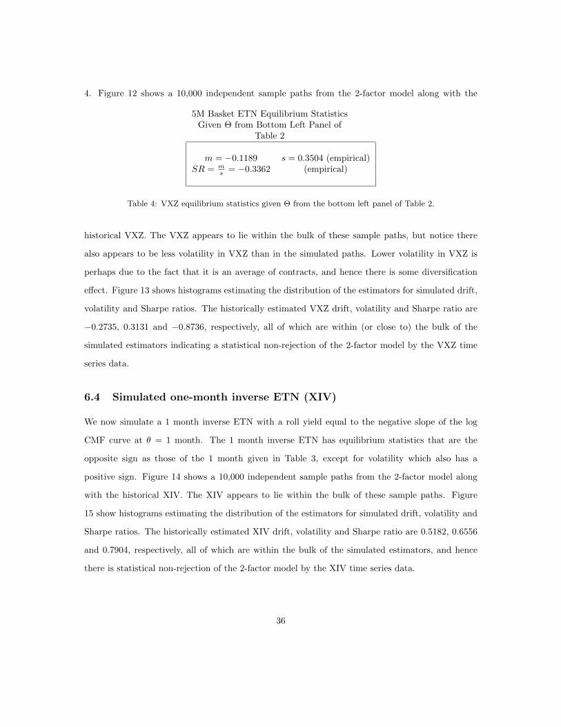
Table 4: VXZ equilibrium statistics given Θ from the bottom left panel of Table 2.
historical VXZ. The VXZ appears to lie within the bulk of these sample paths, but notice there
also appears to be less volatility in VXZ than in the simulated paths. Lower volatility in VXZ is
perhaps due to the fact that it is an average of contracts, and hence there is some diversification
effect. Figure 13 shows histograms estimating the distribution of the estimators for simulated drift,
volatility and Sharpe ratios. The historically estimated VXZ drift, volatility and Sharpe ratio are
−0.2735, 0.3131 and −0.8736, respectively, all of which are within (or close to) the bulk of the
simulated estimators indicating a statistical non-rejection of the 2-factor model by the VXZ time
series data.
6.4 Simulated one-month inverse ETN (XIV)
We now simulate a 1 month inverse ETN with a roll yield equal to the negative slope of the log
CMF curve at θ = 1 month. The 1 month inverse ETN has equilibrium statistics that are the
opposite sign as those of the 1 month given in Table 3, except for volatility which also has a
positive sign. Figure 14 shows a 10,000 independent sample paths from the 2-factor model along
with the historical XIV. The XIV appears to lie within the bulk of these sample paths. Figure
15 show histograms estimating the distribution of the estimators for simulated drift, volatility and
Sharpe ratios. The historically estimated XIV drift, volatility and Sharpe ratio are 0.5182, 0.6556
and 0.7904, respectively, all of which are within the bulk of the simulated estimators, and hence
there is statistical non-rejection of the 2-factor model by the XIV time series data.
36

18-M
ar-
2010
15-M
ar-
2011
12-M
ar-
2012
12-M
ar-
2013
10-M
ar-
2014
06-M
ar-
2015
03-M
ar-
2016
01-M
ar-
2017
10-2
10-1
100
101
102
103
104
Simulated 5 Month Basket ETN
Historical VXZ
Figure 12: The simulated 5 month basket ETN along with the historical VXZ. The VXZ appears to lie
within the bulk of these sample paths.
7 Conclusion
We quantified the statistical behavior of VIX constant-maturity-futures in terms of a stochastic
model and showed how the time-series of ETP prices depend on the volatility of the CMF curve
as and as its slope. Since volatility is often viewed as a stationary, or mean reverting, and the
term-structure of CMF is typically in contango, shorting volatility via ETPs should be profitable,
in principle. In this paper, we are able to quantify the profitability of selling VIX through ETPs.
The results show that although, historically, such strategies have been profitable, the Sharpe ratios
achieved are relatively modest (les than the Sharpe ratio for holding the S&P 500). This is due to
the spikes in VIX accompanied by CMF backwardation which occur sporadically, but inevitably, in
the volatility market.
37

-2 -1.5 -1 -0.5 0 0.5 1 1.50
50
100
150
Estimated 5M Basket ETN Annualized Drift
0.33 0.34 0.35 0.36 0.37 0.380
20
40
60
80
100
120
140
Estimated 5M Basket ETN Annualized Volatility
-6 -4 -2 0 2 40
50
100
150
Estimated 5M Basket ETN Sharpe Ratios
Figure 13: Top Left: The histogram of estimated drifts for the simulated 5M basket ETNs with equal
weight of 1/3 in the 4,5 and 6 month CMFs. Historically, the 5M basket ETN VXZ recorded an estimated
drift of m = 1N∆t
∑`
∆XIVt`XIVt`
= −0.2735 between 3/1/2010 and 3/1/2017, which is within the bulk among
simulated drift estimators. Top Right: For the same time period the historically estimated volatility
for the VXZ was s =
√1
N∆t
∑`
(∆ln(VXZt`) − ∆ln(VXZ)
)2
= 0.3131, which is at the near the bulk of
simulated volatility estimators. Bottom: The historically estimated VXZ Sharpe ratio m/s = −0.8736,
which is within the bulk among simulated Sharpe ratio estimates.
References
[Ben14] C. Bennett. Trading Volatility: Trading Volatility, Correlation, Term Structure and
Skew. CreateSpace Independent Publishing Platform, 99 edition, 2014. ISBN-10:
1461108756, ISBN-13: 978-1461108757.
[Ber05] L. Bergomi. Smile dynamics II. Risk, pages 67–73, Oct 2005.
[Ber08] L. Bergomi. Smile dynamics III. Risk, pages 90–96, Oct 2008.
38

30-N
ov-2
010
25-N
ov-2
011
26-N
ov-2
012
21-N
ov-2
013
19-N
ov-2
014
17-N
ov-2
015
14-N
ov-2
016
10-2
100
102
104
106
Simulated 1 Month invETN
Historical XIV
Figure 14: The simulated 1 month inverse ETN along with the historical XIV. The XIV appears to lie
within the bulk of these sample paths.
[Ber16] L. Bergomi. Stochastic Volatility Modeling. A Chapman et Hall book. CRC Press, 2016.
[BGK13] C. Bayer, J. Gatheral, and M. Karlsmark. Fast Ninomiya-Victoir calibration of the
double-mean-reverting model. Quantitative Finance, 13(11):1813–1829, 2013.
[Whaley1993] Whaley, Robert E., Derivatives on Market Volatility: Hedging Tools Long Overdue,
Fall 1993 The Journal of Derivatives 1 , pp. 7184
[CBOE] The Chicago Board Options Exchange The CBOE Volatility Index - VIX August 2014
http://www.cboe.com/micro/vix/vixwhite.pdf
[Dobi] Dobi, Doris. Modeling Systemic Risk in The Options Market May 2014 PhD Thesis,
Courant Institute of Mathematical Sciences, New York University
[Laloux et al.] Laloux, L., Cizeau, P., Potters, M., Bouchaud, J-P., Random Matrix Theory and
Financial Correlations 2000 Mathematical MOdels and Methods in Applied Science
39

-2 -1 0 1 2 30
50
100
150
Estimated 1M invETN Annualized Drift
0.6 0.62 0.64 0.66 0.68 0.70
20
40
60
80
100
120
140
Estimated 1M invETN Annualized Volatility
-3 -2 -1 0 1 2 3 4 50
20
40
60
80
100
120
140
160
Estimated 1M invETN Sharpe Ratio
Figure 15: Top Left: The histogram of estimated drifts for the simulated 1M inverse ETNs. Historically,
the 1M inverse ETN XIV recorded an estimated drift of m = 1N∆t
∑`
∆XIVt`XIVt`
= 0.5182 between 11/30/2010
and 3/1/2017, which is within the bulk among simulated drift estimators. Top Right: For the same time
period the historically estimated volatility for the XIV was s =
√1
N∆t
∑`
(∆ln(XIVt`) − ∆ln(XIV)
)2
=
0.6556, which is within the bulk among simulated volatility estimators. Bottom: The historically estimated
XIV Sharpe ratio m/s = 0.7904, which is within the bulk among simulated Sharpe ratio estimates.
[LS] Litterman R., Scheinkman J., Common Factors Affecting Bond Returns June 1991 THe
Journal of Fixed Income p. 54
[CIR1985] Cox, J.C., Ingersoll, J.E., and Ross, S.A., A theory of the term structure of interest
rates March 1985 Econometrica Vol 53 N. 2, 385-408
[ETNs] VIX ETF and ETNs list http://www.macroption.com/vix-etf-etn-list/
[CK13] C.Alexander and D. Korovilas. Volatility exchange-traded notes: curse or cure? Journal
of Alternative Investments, 16(2):52–70, 2013.
40

[CW09] P. Carr and L. Wu. Variance risk premiums. The Review of Financial Studies, 22:1311–
1341, March 2009.
41