Folker H. Wittmann, I Zdenek P. Bazant, 2 Fermin Alou, 3 and lin-Keun Kim 4

Statistics of Shrinkage Test Data

REFERENCE: Wittmann, F. H., Briant, Z. P., Alou, F., and Kim, l.·K., "Statistics o( Shrinkage Test Data," Cement. Concrete. and Ag­gregates. CCAGDP, Vol. 9, No.2, Winter 1987, pp. 129-153.

ABSTRACT: A large series of concrete shrinkage tests which can be used for statistical purposes is reported. The series involves two groups of 36 identical cylindrical specimens. with a diameter of 83 mm for Group I and 160 mm for Group 2. Statistical analysis of shrinkage strains and strain rates is presented, and the goodness of fit by normal distribution. log-normal distribution. and gamma distribution is ana­lyzed. Correlations between the values at various times are determined.

The study reveals only the intrinsic randomness of the shrinkage pro­cess (along with measurement errors) and omits the superimposed un­certainties due to randomness of environment and to prediction uncer­tainties in the influence of material composition. curing. and other factors. It is found that the coefficient of variation of shrinkage values first decreases with time and then levels off at 6 to 9'l70. The normal. log­normal. and gamma distributions all give acceptable fits of the ob­served distributions. There are small systematic deviations from normal distribution: the distributions are slightly skewed to the right and slightly platykurtic. The skewness is more pronounced for the distribu­tion of shrinkage rates, and asymmetric distributions such as gamma give slightly better fits. The correlation of single specimen shrinkage deviations from the group mean at various times is characterized by cor­relation coefficients. Their value is found to decrease slowly as the length of the time interval increases. For shrinkage rates, this decrease is much faster. The standard deviation of the single specimen shrinkage from its smoothed shrinkage curve is much less than (about one third of) the standard deviation of the single specimen relative to the mean for all specimens. The standard deviation of all single-specimen smoothed shrinkage curves at one time is almost the same as (about 95'l70 of) the standard deviation of the original un smoothed data for that time.

KEYWORDS: concrete. cements, shrinkage. drying, tests, measure­ments, statistics, probabilistic analysis, random errors. shrinkage prediction

Predictions of shrinkage of concrete have a large statistical vari­ability, which is caused: (1) by the uncertainty in the influence of the composition and curing history of concrete; (2) by the random variability of environment; and (3) by intrinsic randomness of con­crete due to the random nature of the shrinkage mechanism itself and to our uncertainty in the knowledge of the law governing

'Professor, Department of Materials, Swiss Federal Institute of Technol­ogy, Lausanne, Switzerland.

lProfessor. Department of Civil Engineering, Northwestern University, Evanston, IL 60208.

JHead, Concrete Technology and Material Testing Section, Department of Materials, Swiss Federal Institute of Technology, Lausanne, Switzer­land.

'Assistant professor. Department of Civil Engineering, Korea Advanced Institute of Science and Technology, Seoul, Korea; formerly graduate re­search assistant. Northwestern University.

© 1987 by the American Society for Testing and Materials 129

shrinkage. In structural design, each of these three sources of ran­domness should be treated separately [1-6].

The purpose of the present study is to generate statistical data for the third source of randomness, the intrinsic uncertainty. The experimental information on this type of uncertairtty [7-10] is rather limited, and no sufficiently large series of test data which would permit extracting reliable statistics seems to exist. There­fore, a large series of concrete shrinkage tests has been carried out in Lausanne under a cooperative project between the Department of Materials of the Swiss Federal Institute of Technology and the Center for Concrete and Geomaterials at Northwestern University. The purpose of this paper is to report the test results and present their statistical analysis, whose concept was developed in Bazant's report [11]. Two preceding papers [I2.13) used the same data to study the problems of extrapolation of short-time shrinkage data by regression and by Bayesian analysis.

Description of Tests

The experimental study involved one series of 35 cylindrical specimens of diameter 160 mm and another series of 36 cylindrical specimens of diameter 83 mm (Fig. O. (The effect of specimen size, however, is not analyzed here since this has been done in preceding papers [12,13).) The length of each cylinder was double its diameter. The mean standard cylindrical 28-day strength of the concrete was!: = 33.2 MPa (4814 psi) and its modulus of elastic­ity (according to DIN 1045) at 28 days was 36.3 kN/mm2. No ad· mixtures, plasticizers, or air-entraining agents were used. The spe­cific mass of concrete was 2418 kg/ mJ , and 1 mJ contained 350 kg of cement, 168 kg of water, 608 kg offine sand from 0 to 4 mm size, 399 kg of coarse sand from 4 to 8 mm size, 399 kg of fine gravel from 8 to 16 mm size, and 494 kg of coarse gravel from 16 to 31.5 mm size. The corresponding volume fractions were 0.113, 0.168,0.226,0.148,0.148, and 0.184, respectively, plus 0.013 for air. The cement (of type CPN from the plant at Eclepens near Lau­sanne) was approximately of ASTM Type I, with fineness defined by surface area 2900 m2/g (Blaine). All aggregate was from a gla· cial moraine, of rounded shapes. Mineralogically, all aggregate was composed of 40 to 46% calcite, 29 to 32% quartz, 8 to 13% residue of crystalline rocks of multimineral composition, predomi­nantly quartzitic, and 12 to 18% of composite grains, essentially quartzitic. All the specimens were cast from one batch of concret~. The specimens were cured in a sealed state and were kept sealed In

their molds (made of PVC) until the instant of exposure to the dry· ing environment. This type of curing is preferable to curing in wa· ter bath, which has recently been found to cause nonuniform water intake, significant swelling stresses, and microcracking. The envi·

0149-6123187/0012-0129$02.50

130 CEMENT, CONCRETE, AND AGGREGATES

hinge

spring (force 60N)

.... axial .. defomation

gauge

specilllen (0 = 83 mm or 160 111m, height = 20)

- metallic base

FIG. I-Photographs oj test specimens and laboratory setup.

ron mental humidity was 6S ± 5 0/0. and the room temperature was 18 ± 1°C throughout the casting, curing, and shrinkage.

The shrinkage deformations were measured by taking length readings between the ends of the specimens along the cylinder axis. The deformations of all specimens were measured with one dial gauge which had contacts made of steel balls that fit into ring­shaped steel targets glued to the specimens. To be able to record the very initial shrinkage, the targets for deformation measure­ments had been attached before the molds were stripped. All speci­mens were exposed to drying at the age of seven days and shrinkage measurements started immediately. The initial reading, represent­ing the zero strain for Tables 1 and 2, was taken within 1 min after the stripping of the mold (it is important to take the first reading promptly; in previous tests the first reading was apparently taken much later, causing a significant initial shrinkage to go unre­corded),

Statistics for the Group of Specimens and Their Evolution with Time

The shrinkage strains Esh measured for specimens i = 1. 2, , , . , N are reported in Table 1 (for diameter 83 mm, N = 36) and Ta-

ble 2 (for 160 mm, N = 35) in terms of their mean f, at time t, (r = 1.2.3, ...• n) and the deviations from the mean. Ei., - f,. where Ei., is the shrinkage strain Esh of specimen number i at time l,. Time l. represents the duration of drying. Line 38 gives the standard de­viation s, of the set of all Ei.,-values at time t,; s, = I:;[(Ei., - f,)2/ (N - 1)]1/2 where N - 1 is used instead of N to obtain an unbiased estimate [14.15). Line 39 gives the coefficient of variation w, = s,lf, of the values Ei.,' Considering that in theory an infinite num­ber of samples could be cast and that the available N specimens represent a sample drawn from this infinite popUlation, the stan­dard deviation and the coefficient of variation of the mean value f, are s,/.JN and w,I.JN/14-16] (.IN = 6 or 5.92).

Lines 40-43 give the mean If of the values of log Ei." the values of 10'!-, the standard deviation sf of these values, and their coefficient of variation wf. These characteristics may be used for determining the log-normal distribution of shrinkage strains, which has the ad­vantage that it does not admit negative shrinkage strain values which are physically impossible (if measurement error is elimi­nated).

Another distribution which does not permit negative strain val­ues and is in a certain sense better justified physically (17) is the gamma distribution of strain. It has the probability density j(E) =

IJ-oEo-le-'/~ Ir(a) for E > 0 (and 0 for E < 0), where r(a) is the gamma function, that is, r(a) = 10' Eo-le-'dE, a is the scale pa­rameter and IJ is the shape parameter (a > 0, IJ > 0). As is well known [18], the mean and standard deviation of the gamma distri­bution are l' = a(J and s = (J.Jix. From this itfollows that a = (1',1 S,)2, IJ = s; IE,; these parameters are evaluated for the present data on Lines 44 and 45.

As measures of the deviations from the normal distributions of Ei." lines 46 and 47 list the skewness, m, and the kurtosis, k, de­fined for time t, as in Ref 14. p. 62

1 II N J m=- - r: k -e)3 s~ N ;=1 I.' , and

1 II N J k = - - r: k - l' )4 s: N ;=1 I.' , (1)

Note that for normal distributions m = 0 and k = 3. When k > 3, the distribution is leptokurtic (that is, it has a sharp peak and long tails), and for k < 3, the distribution is platykurtic (that is, it has a flat peak and short tails, a shape reminding of the platypus). Lines 48 and 49 give the skewness m L and kurtosis kL for the distribution of log Ei." which indicates deviations from the log-normal distribu­tion of shrinkage strain.

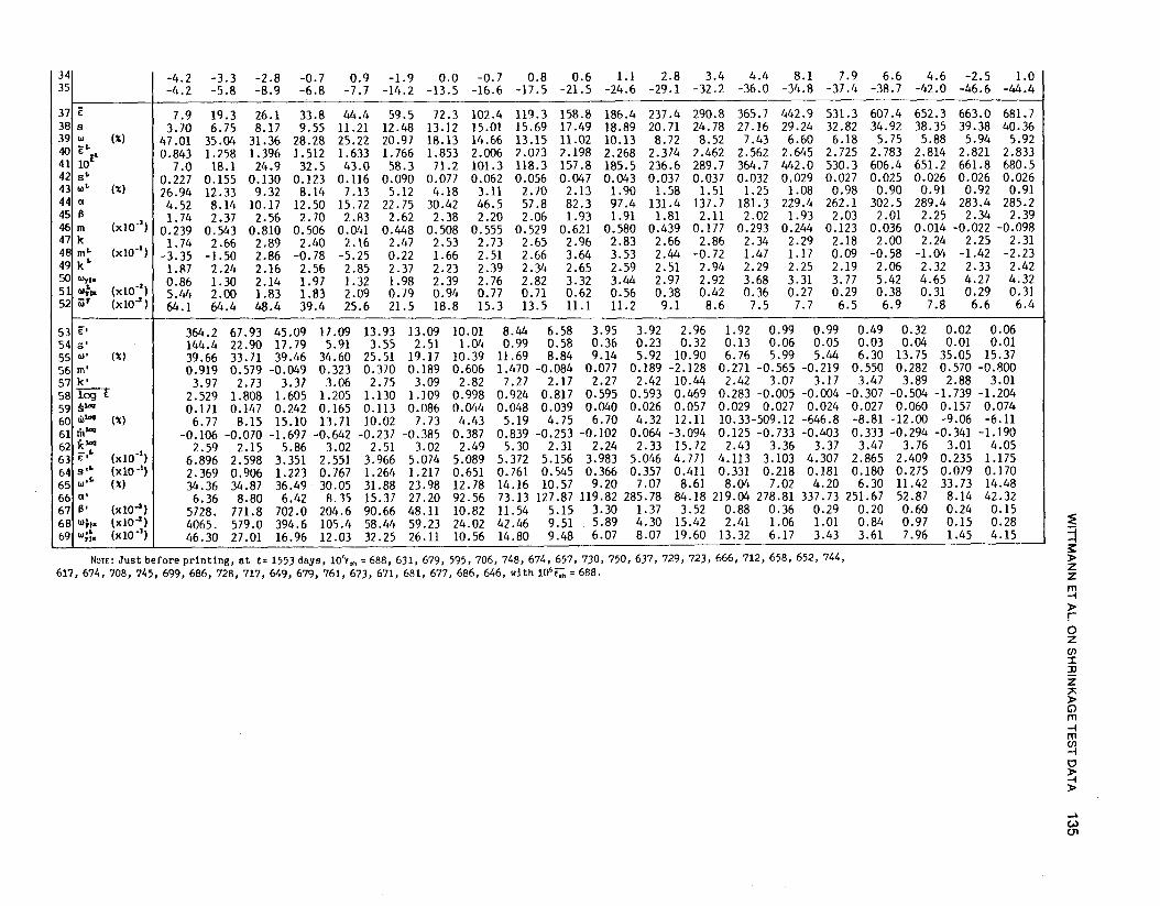
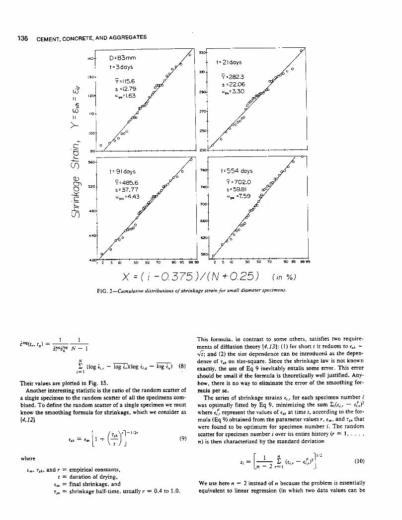
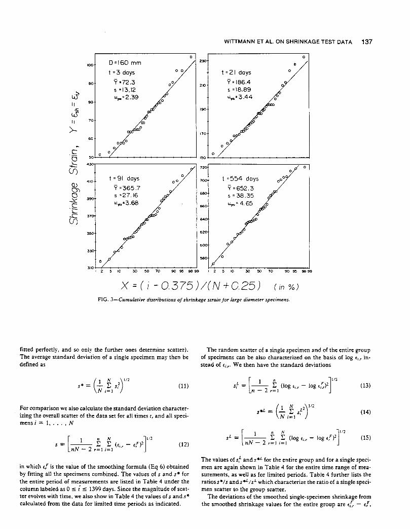
To evaluate the goodness of fit by various distributions, Figs. 2-3 show for the two groups of N specimens (N = 36 or 35) the cumulative frequency distributions of the Ei., values. Among the various types of cumulative frequency distribution plots we chose the plot introduced by Blom and Kimball [16.19.20], which was proven to be optimum. For this plot, the plotting positions are (i -0.375)/(N + 0.25), which is superior to either (i - 0.5)/N or iI (N + 1) as customarily used (i is the number of data values :S Ei.r>. Figures 2-3 show these cumulative plots for the actual shrinkage strains Ei., (at four different times t, = t - to, and for both speci­men diameters D). Figures 4-5 show the same for log Ei.,' If the distributions of Ei., or log Ei., were normal and perfect, then the plots would have to be straight lines. Thus, vertical deviations from the least-square fit by a straight line represent errors. These errors are characterized by their coefficients of variation wYIX and wi1x, listed on lines SO-51 of Tables 1-2, pertaining to the normal and log-normal distributions, respectively.

For the modeling of shrinkage as a stochastic process with inde­pendent increments, which is theoretically superior to the model­ing of shrinkage as a stochastic process with independent total shrinkage values at subsequent times [17], it is useful to know the statistics of the shrinkage increments. They may be characterized by the statistics of the shrinkage rates, which may be approxi­mately calculated for specimen number i as

Ei., = Ei., - Ei.,-I (at time .Jt,_lt,) tr - tr-I

(2)

The rate estimated from interval (t,_I' t,) is best referred to the center of the interval in log t-scale, which is .Jt,_lt,. Lines 53-57 of the tables give for the entire group of specimens (i = I, ... , N) the mean of the shrinkage rates e:, their standard deviation s: , their coefficient of variations w:, skewness m:, and kurtosis k: . Furthermore, lines 58-62 give the statistics of log Ei." that is, their mean log E" standard deviation s~og, coefficient of variation w~og, skewness m~01, and kurtosis k~og.

WITTMANN ET AL. ON SHRINKAGE TEST DATA 131

Since the initial evolution of shrinkage is simpler in the log-log plot, it is also useful to consider the rates of log E,h in log t, calcu­lated as

log Ei.r - log Ei.,-I E/f = --''-------'--­

log t, - log tr-I (3)

Their mean e: L, standard deviation s; L, and coefficient of varia­tion w; L are listed in lines 63-65. Furthermore, lines 66-67 give the scale parameter a' and the shape parameter IJ' for the gamma distribution of shrinkage rates Ei." determined as a' = (l: Is:)2 andIJ' =s;2Il:.

Figures 6-9 help to evaluate the goodness of fit of the shrinkage rates by the normal and log-normal distributions. These figures show the cumulative frequency distributions of fi., and E/f, plotted in the same manner as Figs. 2-5. If these distributions were per­fect, these plots would have to be straight lines, and so the vertical deviations from the straight-line fit are a measure of the deviation from the theoretical distribution. These vertical deviations may be characterized by their coefficients of variation wYIX and wyfx for the normal and log-normal distributions, respectively, which are listed in lines 68-69.

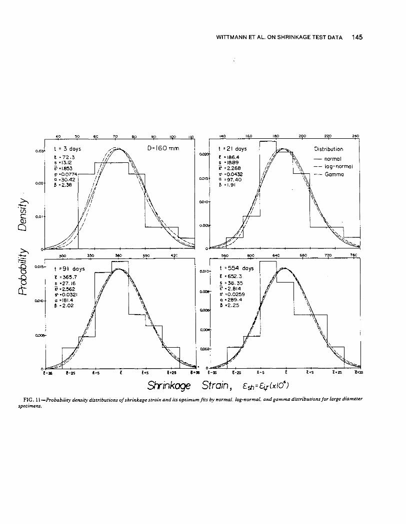
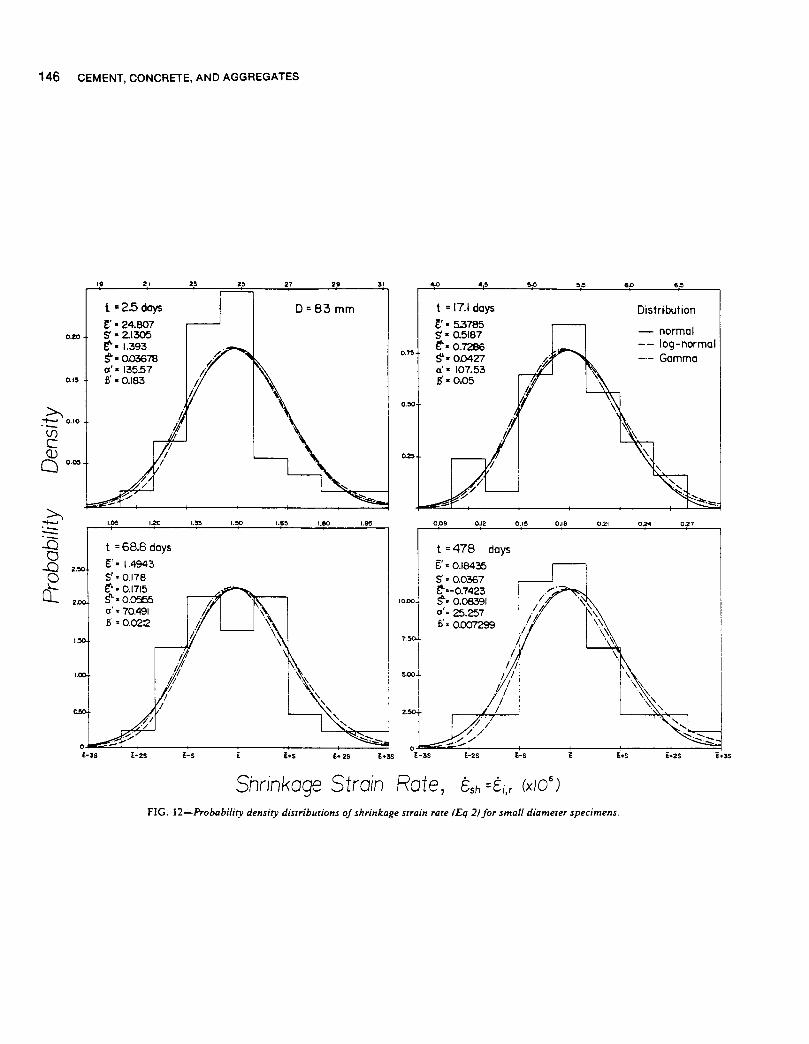
The probability density distributions corresponding to the afore­mentioned cumulative distributions are plotted in Figs. 10-13.

Statistics of the Time Series

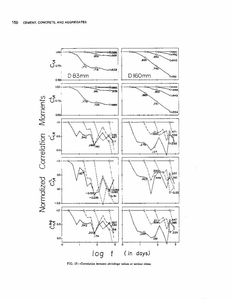
Aside from the statistics for each group of specimens at a fixed time, it is also of interest to determine correlation of shrinkage strains at various times for each particular specimen. This correla­tion may be characterized, for example, by the correlation coeffi­cient [Ref 14. p. 74; Ref 15. p. 161] for Esh and log Esh at two differ­ent times t, and tq , which is obtained as the covariance divided by the product of standard deviations, that is,

cL(t" tq ) = _1 ___ 1_ f (log Ei., - ef)(log Ei.q - l~) (5) sfs~ N - 1 ;=1

We use here N - 1 instead of N in the usual definition [14.15] because we must require that for tq = tr the value of c be 1.0 (per­fect correlation). The values of these correlation moments for all possible combinations of shrinkage times 3,21,91,554, and 1399 days are listed in Table 3. A correlation coefficient equal to 1.0 means perfect correlation (functional dependence) and 0 means no correlation. The rates in this table are calculated from the intervals (2,3), (14, 21), (52, 91), (412,554), and (1105,1399) (in days). The autocorrelation function of the random process of shrinkage could be constructed from Table 3.

The normalized correlation moments can be similarly defined for the deviations of the single specimen shrinkage rates from the group mean

'( )_ 1 1 ~ (. __ ')(' __ ') c t r , tq - -. -, --- J."J €j,r Er fi.1/ {q S,Sq N - 1 ;=1

(6)

(7)

time t .0104 0.042 (in days)

1 -3.5 5.1 2 3.9 -2.3 3 -2.2 -7.2 4 -1.0 -2.3 5 2.7 0.2 6 -5.9 -12.1 7 7.6 7.5 8 -2.2 -3.5 9 -3.5 -3.5

10 -2.2 -4.7 11 -3.5 -4.7 12 -2.2 -7.2 13 -1.0 0.2 14 -2.2 -3.5 15 -10.8 -9.6 16 -9.6 -6.0 17 t.t\ - C eh 1.4 0.2 18 3.9 5.1 19 -3.5 -3.5 20 -9.6 -8.4 21 -1.0 1.4 22 -2.2 -2.3 23 -9.6 -6.0 24 -5.9 -1.1 25 3.9 6.3 26 10.0 2.6 27 10.0 10.0 28 1.4 0.2 29 7.6 5.1 30 5.1 5.1 31 7.6 7.5 32 0.2 2.6 33 12.5 13.7 34 5.1 10.0

TABLE I-Shri"kag<, strai"s m('(lSl/red for illdividl/al specime"s alld their statistics (D = 83 mm) (f,h X 10").

0.208 0.375 1 2.08 3 6 8 14 21 34 52 91 169 258 412 554 1105 13991

-1.0 -4.1 -2.8 0.3 3.3 5.5 8.1 15.2 18.0 26.1 28.6 18.1 13.1 26.5 22.7 29.6 29.9 32.3 1 -8.4 -12.6 -13.8 -18.1 -22.4 -26.4 -27.4 -30.2 -29.8 -33.9 -41.3 -49.3 -67.8 -74.0 -79.0 -85.6 -91.4 -85.3 -9.6 -1l.4 -8.9 -7.0 -7.7 -8.0 -10.3 -9.3 -10.2 -15.6 -24.1 -35.8 -49.4 -51. 9 -53.3 -48.8 -44.8 -42.5 -3.5 -5.3 -2.8 -2.1 -1.6 1.8 2.0 5.4 5.7 5.3 4.1 1.0 -5.3 -4.1 -3.0 -5.9 -1.9 -3.2 -3.5 -6.5 -5.2 -4.6 -2.8 0.6 0.7 0.5 0.8 -3.3 -9.4 -17.4 -24.9 -26.2 -27.5 -30.4 -22.8 -24.1

-13.3 -9.0 -6.5 -2.1 -1.6 4.3 5.7 15.2 21.7 23.7 28.6 24.2 29.0 40.0 37.4 46.8 43.4 53.1 7.6 8.2 10.7 10.1 9.4 6.7 4.4 5.4 5.7 2.8 -0.8 -6.4 -12.7 -15.1 -16.5 -19.4 -15.4 -14.3 I

-2.2 -2.8 5.8 16.2 20.5 27.5 30.2 44.6 49.8 59.2 71. 5 78.2 80.5 95.1 102.4 106.8 103.5 108.3 i

-5.9 -6.5 -1.6 4.0 9.4 16.5 17.9 27.4 30.2 34.7 39.6 35.3 40.0 48.6 54.6 55.4 49.5 59.3 -12.1 -12.6 -13.8 -15.6 -16.3 -17.8 -18.9 -19.1 -22.5 -26.6 -32.7 -38.3 -51.9 -56.8 -60.6 -66.0 -64.4 -63.3 -10.8 -13.9 -15.0 -14.4 -15.1 -19.0 -21.3 -24.0 -26.1 -31.5 -36.4 -37.0 -48.2 -51.9 -52.0 -52.5 -49.7 -52.3

1 -13.3 -17.5 -21.2 -23.0 -21.2 -15.4 -16.4 -10.6 -6.5 -7.0 -6.9 -10.1 -13.9 -13.9 -16.5 -18.2 -16.6 -20.4 -1.0 -1.6 -1~.0 -5.8 -5.3 -0.6 0.7 1.7 3.3 6.5 5.3 9.5 13.1 17.9 19.0 18.6 23.8 20.1 -4.7 -7.7 -12.6 -18.1 -20.0 -25.2 -31.1 -37.5 -40.8 -47.4 -59.6 -68.9 -78.8 -91.1 -96.2 -97.8 -95.1 -97.6 -7.1 -9.0 -4.0 -2.1 -1.6 1.8 3.2 11.5 18.0 26.1 37.2 27.9 56.0 69.4 80.3 83.5 87.5 83.8 -4.7 -5.3 -6.5 -5.8 -7.7 -11. 7 -14.0 -16.7 -18.8 -22.9 -30.2 -35.8 -44.5 -54.4 -59.4 -63.5 -68.1 -64.5 2.7 2.1 4.6 5.2 4.5 3.0 0.7 1.7 3.3 4.1 4.1 4.6 3.3 3.2 3.1 2.7 4.2 1.7 3.9 4.5 9.5 13.8 14.3 17.7 20.4 23.8 27.8 37.1 43.3 50.0 58.4 64.5 73.0 72.5 69.1 69.1

-3.5 -5.3 -6.5 -9.5 -10.2 -15.4 -20.1 -22.8 -26.1 -37.6 -46.2 -54.2 -64.1 -75.2 -81.5 -90.5 -90.2 -91. 5 -8.4 -7.7 -5.2 -3.4 -2.8 -3.1 -4.2 -2.0 0.8 2.8 9.0 18.1 26.6 32.6 39.9 39.4 43.4 39.7 1.4 4.5 7.0 8.9 8.2 10.4 13.0 20.1 25.3 31.0 42.1 48.7 56.0 59.6 64.4 63.9 65.5 66.6

-4.7 -5.3 -7.7 -13.2 -16.3 -25.2 -31.1 -40.0 -47.0 -59.7 -73.1 -76.3 -92.3 -109.5 -115.8 -124.8 -128.2 -123.3 -7.1 -7.7 -8.9 -9.5 -9.0 -0.6 0.7 6.6 9.4 9.0 17.6 34.0 36.4 38.8 38.6 38.2 38.5 36.0 -5.9 -6.5 -15.0 -19.3 -18.8 -20.3 -21. 3 -24.0 -23.7 -30.3 -30.2 -28.5 -18.8 -28.6 -31.2 -35.3 -33.8 -33.9 7.6 7.0 3.3 1.5 3.3 9.2 11.8 16.4 19.2 32.2 45.8 58.6 71.9 82.9 88.9 94.6 90.0 89.9 1.4 3.3 3.3 1.5 -0.4 -1.9 -0.5 -2.0 -1.6 5.3 11.4 18.1 27.8 36.3 41.1 45.5 39.7 44.6

14.9 15.6 14.4 13.8 11.9 6.7 6.9 0.5 -2.9 -3.3 -6.9 -7.6 -11.4 -15.1 -14.1 -17.0 -16.6 -21.6 3.9 4.5 -0.3 -5.8 -7.7 -14.1 -15.2 -26.5 -33.5 -40.1 -49.8 -53.0 -58.0 -67.8 -71. 7 -75.8 -80.4 -81.7 7.6 8.2 5.8 6.4 5.8 3.0 4.4 -2.0 -4.1 -2.1 -3.3 -1.5 -1.6 -4.1 -4.3 -7.1 -5.6 -8.1

10.0 11.9 11.9 11.3 9.4 7.9 10.6 7.8 8.2 15.1 20.0 21.8 30.2 33.9 33.7 33.3 36.0 31.1 8.8 9.4 8.2 8.9 9.4 9.2 10.6 5.4 4.5 5.3 7.8 14.4 25.3 25.3 26.4 30.8 27.5 26.2 6.3 13.1 14.4 16.2 19.2 20.2 22.8 22.5 22.9 32.2 35.9 43.8 54.7 58.4 58.2 73.7 75.3 71. 5

21.0 21. 7 18.0 16.2 15.6 15.3 16.7 11.5 9.4 6.5 4.1 8.3 11.8 10.6 11.7 13.7 15.2 13.9 14.9 19.2 21.7 24.8 25.4 23.9 26.5 25.0 24.1 26.1 31.0 37.7 49.8 51.0 46.0 55.4 49.5 54.4

..... (..) I\)

(') m 3: m Z .-1 (') o z (') :0

~ .m > z o > G> G> :0 m G>

~ m en

351

7.6 11.2 16.1 19.2 19.3 18.7 18.0 16.5 17.9 11.5 5.7 0.4 -2.0 1.0 -0.4 -5.3 -7.9 -12.1 -11.7 -14.3 36 -8.4 -6.0 2.7 5.8 4.6 1.5 0.9 -3.1 -4.2 -13.0 -20.0 -30.3 -33.9 -33.4 -39.6 -49.5 -50.8 -53.7 -54.6 -59.6

37 r 15.7 26.8 35.3 44.5 61.6 92.8 115.6 162.4 188.0 244.6 282.3 351.3 427.3 485.6 540.8 629.1 675.8 702.0 716.4 718.9 38 s 6.11 6.35 8.81 10.28 10.78 12.16 12.79 14.42 16.38 19.63 22.06 27.56 33.86 37.77 45.80 52.78 56.16 59.81 59.52 59.76 39 w (X) 38.87 23.71 24.92 23.11 17.49 13.10 11.06 8.88 8.71 8.02 7.81 7.85 7.92 7.78 8.47 8.39 8.31 8.52 8.31 8.31 40 rL 1.159 1.416 1.535 1.637 1.783 1.964 2.060 2.209 2.272 2.387 2.449 2.544 2.629 2.685 2.732 2.797 2.828 2.845 2.854 2.855 41 lOEL 14.4 26.1 34.3 43.4 60.7 92.0 114.9 161.8 187.3 243.8 281.4 350.3 426.0 484.1 538.9 626.9 673.5 699.5 714.0 716.5 42 SL 0.194 0.105 0.107 0.099 0.077 0.058 0.049 0.039 0.038 0.035 0.034 0.035 0.035 0.034 0.037 0.037 0.037 0.038 0.037 0.037 43 wL

16.72 7.40 6.98 6.07 4.31 2.94 2.36 1.77 1.69 1.48 1.40 1.36 1.33 1.27 1.37 1.32 1.29 1.32 . 1.29 1.28 44 (1 6.62 17.79 16.10 18.73 32.68 58.30 81. 71 126.9 131.7 155.4 163.7 162.5 159.3 165.2 139.5 142.1 144.8 137.8 144.9 144.7 45 S 2.38 1. 51 2.19 2.38 1.89 1.59 1.41 1.28 1.43 1.57 1.72 2.16 2.68 2.94 3.88 4.43 4.67 5.10 4.94 4.97 46 m (x10" ) 0.118 0.276 0.495 0.435 0.173 0.019 -0.005 -0.170 -0.234 -0.158 -0.170 -0.170 -0.156 -0.131 -0.186 -0.195 -0.163 -0.167 -0.240 -0.180 47 k 2.12 2.16 2.38 2.13 2.12 2.05 2.03 2.10 2.10 2.42 2.43 2.29 2.26 2.17 1.95 1.98 2.01 1.99 2.05 1.98 48 mL (xlO") -6.99 -1.69 0.72 0.84 -1.44 -2.01 -1.83 -3.17 -3.78 -3.28 -3.37 -3.24 -3.10 -2.72 -3.11 -3.23 -2.95 -3.01 -3.75 -3.08 49 kL 2.75 2.32 2.10 2.03 2.22 2.10 2.03 2.12 2.16 2.42 2.45 2.34 2.32 2.20 2.02 2.07 2.09 2.08 2.16 2.06 50 W,.I_ 1.01 0.92 1.64 2.16 1.41 1.46 1.63 2.25 2.61 2.77 3.30 4.58 4.57 4.43 6.65 7.51 6.99 7.59 8.44 7.84 51 w~l. (xlO-l) 5.06 1.27 1.24 1.58 0.97 0.77 0.69 0.70 0.71 0.57 0.58 0.63 0.54 0.47 0.61 0.60 0.53 0.55 0.61 0.55 52 t;:.r (xlO") 68.9 54.6 28.1 24.2 19.9 13.8 11.1 8.9 8.8 8.3 8.0 7.9 8.9 7.9 10.6 8.5 8.5 8.9 8.3 8.4

53 E' 354.0 51. 27 54.94 27.40 28.81 24.81 15.61 12.78 9.44 5.38 5.31 4.22 1.49 0.71 0.99 0.30 0.18 0.03 0.01 54 s' 107.9 23.68 14.76 5.35 3.05 2.13 1.43 1.20 0.99 0.52 0.49 0.39 0.18 0.13 0.09 0.03 0.04 0.01 0.01 55 w' (X) 30.4846.19 26.86 19.54 10.60 8.59 9.15 9.39 10.47 9.64 9.28 9.24 11. 91 18.12 8.99 9.40 19.90 25.28 156.0 56 m' -0.076 0.074 0.534 0.053 0.636 0.561 0.170 -0.853 0.310 -0.198 0.051 0.078 0.256 0.333 -0.004 0.672 0.772 -0.158 0.851 57 k' 3.07 2.36 3.15 3.26 4.04 3.68 2.09 2.99 2.46 2.37 2.14 2.10 2.23 2.87 2.25 2.59 3.60 1.94 2.89 58 log €: 2.525 1.647 1.725 1.429 1.457 1.393 1.192 1.105 0.973 0.729 0.724 0.623 0.171 -0.156 -0.005 -0.520 -0.742 -1.598 59 ~l .. 0.155 0.265 0.118 0.090 0.045 0.037 0.040 0.043 0.045 0.043 0.041 0.040 0.052 0.079 0.02·9 0.040 0.084 0.118

* *

60 w10lJ (X) 6.14 16.07 6.84 6.28 3.10 2.64 3.33 3.89 4.65 5.86 5.60 6.46 30.07 -50.53 -742.1 -7.67 -11.30 -7.39 * 61 m"'" -1.078 -1.125 -0.198 -0.734 0.25/• 0.249 0.009 -1.057 0.091 -0.402 -0.121 -0.083 0.053 -0.099 -0.186 0.511 0.195 -0.485 62 k"'" 3.96 3.67 2.76 i •• 31. 3.31 3.50 2.17 3.52 2.36 2.50 2.22 2.13 2.05 2.43 2.35 2.39 3.00 1.92 63 CIL (xlO") 4.267 1.709 3.990 3.426 5.674 6.076 4.939 5.086 4.717 3.535 4.542 4.605 2.287 1.733 3.575 1.532 1.277 0.296

* *

0.015 64 S,L (x10") 2.069 0.713 1.002 0.855 0.806 0.760 0.528 0.296 0.426 0.260 0.215 0.187 0.221 0.219 0.152 0.090 0.193 0.079 0.233 65 W,L (X) 48.48 41. 72 25.12 24.95 14.21 12.51 10.69 5.81 9.03 7.36 4.73 4.07 9.68 12.63 4.25 5.87 15.08 26.76 154.4 66 (1' 10.77 4.69 13.86 26.18 89.07 135.57 119.41 113.41 91.17 107.53 116.02 117.20 70.49 30.47 123.78 113.08 25.26 15.65 0.41 67 S' (x 10" ) 3289. 1093.7 396.3 10l •. 6 32.35 18.30 13.08 11.27 10.36 5.00 4.58 3.60 2.12 2.33 0.80 0.27 0.73 0.17 68 w',.. (x10"') 2005. 370.6 341.1 109.4 73.84 58.63 24.55 41.77 14.01 8.90 7.02 4.70 2.96 2.32 1.09 0.73 0.94 0.17 69 w '~. (x10" ) 76.69 1/ .. 22 43.86 13.35 12.65 14.92 9.66 4.66 1l.26 3.38 2.72 4.49 3.81 4.96 2.41 2.05 6.49 1. 57

2.11 0.41 6.58

" Some strain rates for this time were negative NOTY.: Just before printing, at t: 1553 days, further readings were taken: 106£,.: 750,636,677,715,698,774,826,824,780,662,666,699,

737,624,804,654,720,790,627,758,788,599,755,686, 807, 761, 698, 639, 710, 751, 745, 793, 733, 774, 704, 660, with 10'f:;;': 723.

:E ~ 3: » z Z m -I » ! 0 z en J: :Il Z ;,,;: » G> m -I m en -I 0 » -I »

..... (.oJ (.oJ

TABLE 2-Slrri,,/w!?e stmi"s measured for i"dividual specimens and tlreir statistics (0 = 160 mm) (t,h X /06).

time t (in days) .0104 0.042 0.142 0.313 1 2.02 3 6 8 14 21 34 52 91 169

1 1.9 1.6 -0.3 -1.9 2.1 3.0 3.6 4.2 3.3 5.5 3.5 5.2 7.0 3.2 2.0 2 -1.8 -4.6 -5.2 -5.6 0.9 -0.7 -1. 3 -0.7 -4.1 -5.6 -9.9 -11.9 -15.0 -22.5 -32.4 3 -3.0 -4.6 -6.4 -10.5 -17.5 -17.9 -17.2 -17.8 -18.8 -17.8 -18.5 -16.8 -13.8 -15.2 -17.6 4 -3.0 1.6 0.9 4.2 7.0 5.4 2.4 -1.9 -5.3 -10.5 -14.8 -20.5 -27.3 -37.3 -49.5 5 3.2 1.6 0.9 3.0 3.4 5.4 4.9 5.5 4.5 6.7 7.2 8.9 10.7 5.6 6.9 6 -1.8 2.8 5.8 9.1 19.3 23.8 24.5 27.5 27.8 31.2 35.4 35.9 42.6 44.9 47.3 7 -4.2 -7.0 -8.9 ':10.5 -13.8 -10.5 -8.6 -5.6 -5.3 -1.9 -0.1 0.3 4.6 -4.2 2.0 8 -0.5 -3.3 -2.8 -4.3 -5.2 -5.6 -7.4 -9.2 -10.2 -10.5 -13.6 -15.6 -16.2 -20.1 -22.5 9 -4.2 0.4 3.4 3.0 5.8 6.7 7.3 9.1 10.6 15.3 17.0 18.7 26.6 32.6 32.6

10 6.8 15.1 20.5 22.6 20.5 28.7 31.8 37.3 38.8 44.7 46.4 49.3 56.1 58.3 62.0 11 -5.4 -9.5 -11.3 -17.8 -23.6 ~22.8 -20.9 -22.7 -23.7 -25.2 -27.1 -31.5 -56.7 -48.3 -39.7 12 5.6 5.3 4.6 -1.9 -7.7 -3.2 -6.2 -4.3 -1.6 3.0 7.2 13.8 19.3 27.7 31.4 13 6.8 10.2 11.9 12.8 13.2 16.5 11.0 11.6 13.1 12.8 12.1 16.2 16.8 24.0 17.9 14 -5.4 -7.0 -6.4 -4.3 -2.8 -1.9 -3.7 -6.8 -6.5 -6.8 -7.5 -5.8 -5.2 -6.6 -7.8 15 -1.8 -2.1 -4.0 -6.8 -4.0 -6.8 -7.4 -6.8 -6.5 -4.3 -3.8 -2.1 2.1 4.4 11.8 16 3.2 -3.3 -6.4 -9.2 -11.3 -11. 7 -14.7 -17.8 -18.8 -17.8 -17.3 -18.1 -21.1 -22.5 -26.2 17 f; ... - i: ... -0.5 -7.0 -7.7 -6.8 -4.0 -5.6 -8.6 -12.9 -15.1 -17.8 -18.5 -20.5 -21.1 -21.3 -25.0 18 1.9 4.0 0.9 -4.3 -8.9 ·6.8 -7.4 -3.1 -2.8 -0.7 2.3 5.2 10.7 21.6 24.0 19 -4.2 -10.7 -10.1 -12.9 -17.5 -16.6 -19.6 -23.9 -24.9 -30.1 -33.2 -37.7 -42.0 -45.8 -53.2 20 1.9 16.3 19.3 17.7 15.6 18.9 17.1 16.5 15.5 15.3 14.6 12.6 11.9 9.3 6.9 21 -4.2 -9.5 -7.7 -8.0 -12.6 -13.0 -14.7 -15.4 -15.1 -11.7 -8.7 -5.8 -1. 5 4.4 9.3 22 4.4 10.2 10.7 14.0 11.9 21.4 24.5 31.2 32.7 38.6 40.3 42.0 48.7 51.0 53.4 23 0.7 -0.9 -1. 5 -0.7 -2.8 -0.7 -3.7 -5.6 -6.5 -8.0 -6.3 -8.3 -6.4 -5.4 -1.7 24 3.2 0.4 -0.3 3.0 5.8 4.2 6.1 6.7 8.2 6.7 7.2 6.4 0.9 -0.5 -5.4 25 -1.8 2.8 4.6 12.8 18.1 16.5 18.3 20.2 19.2 21.4 23.1 22.4 24.2 26.5 28.9 26 -0.5 1.6 0.9 1.8 3.4 0.5 2.4 4.2 11.9 4.2 7.2 10.1 10.7 13.0 15.4 27 -3.0 -7.0 -6.4 -6.8 -6.4 -13.0 -14.7 -17.8 -17.5 -21.5 -22.2 -25.4 -27.3 -32.4 -33.6 28 3.2 7.7 13.2 14.0 11.9 10.3 12.2 10.4 9.4 4.2 -0.1 -2.1 -5.2 -9.1 -12.7 29 -3.0 -7.0 -8.9 -9.2 -8.9 -3.2 3.6 11.6 14.3 20.2 25.6 32.2 35.2 43.6 48.5 30 1.9 0.4 -2.8 -4.3 -2.8 -8.1 -7.4 -10.5 -12.6 -14.1 -14.8 -15.6 -18.7 -21.3 -20.1 31 1.9 -0.9 -4.0 -3.1 -4.0 -9.3 -8.6 -9.2 -9.0 -10.5 -12.4 -11.9 -12.6 -14.0 -14.0 32 4.4 6.5 8.3 7.9 8.3 4.2 7.3 9.1 8.2 6.7 6.0 2.8 0.9 -0.5 -0.5 33 5.6 5.3 7.0 10.4 13.2 7.9 8.5 4.2 3.3 -0.7 -2.6 -5.8 -10.1 -11.5 -ll.5

258 412 554

5.5 4.2 4.6 -42.3 -43.6 -50.6 -16.6 -16.7 -12.6 -61.9 -69.4 -81.2

7.9 6.6 10.7 57.0 54.4 62.1 1.8 -9.3 3.3

-23.9 -24.0 -28.5 38.6 45.8 46.2 63.1 60.5 65.8

-43.5 -42.4 -48.1 41.0 47.1 52.3 19.0 31.1 16.8

-11.7 -14.2 -17.5 16.5 21.3 24.2

-30.0 -35.0 -34.7 -28.8 -32.6 -32.2 30.0 40.9 43.8

-59.5 -63.2 -70.2 3.0 1.7 -5.3

15.3 17.6 20.5 54.5 53.2 53.6 0.6 7.8 7.0

-10.4 -13.0 -15.1 30.0 29.9 30.3 20.2 23.8 26.6

-32.5 -32.6 -35.9 -14.1 -17.9 -16.3 50.8 50.7 68.3

-20.2 -19.1 -13.8 -16.6 -20.3 -20.0

0.6 5.4 -0.4 -14.1 -16.7 -16.3

1105

3.7 -53.9 -9.8

-83.3 14.7 57.6 3.7

-28.2 45.3 63.7

-45.3 52.7 18.4

-20.8 22.1

-38.0 -33.1 45.3

-73.5 -7.4 19.6 55.1 9.8

-6.1 39.2 28.2

-39.2 -14.7 74.8

-17.2 -17.2 -4.9

-12.3

1399

2.2 -56.6 -11.3 -89.7 14.5 58.6 ' 1.0

-32.1 45.1 64.7

-50.5 45.1 18.1

-23.5 24.3

-38.2 -34.6 48.8

-75.0 -8.8 23.0 56.1 10.8 -6.4 41.4 31.6

-37.0 -11.3 75.7

-16.2 -13.7 -2.7

-10.1

..... ~

o m :: m

.~ 8 z o lJ

~ » z o » G> G> lJ m G> ~ rn

34 -4.2 -3.3 -2.8 -0.7 0.9 -1.9 0.0 -0.7 0.8 0.6 1.1 2.8 3.4 4.4 8.1 7.9 6.6 4.6 -2.5 1.0 35 -4.2 -5.8 -8.9 -6.8 -7.7 -14.2 -13.5 -16.6 -17.5 -21.5 -24.6 -29.1 -32.2 -36.0 -34.8 -37.4 -38.7 -42.0 -46.6 -44.4

37 £ 7.9 19.3 26.1 33.8 44.4 59.5 72.3 102.4 119.3 158.8 186.4 237.4 290.8 365.7 442.9 531.3 607.4 652.3 663.0 681. 7 38 5 3.70 6.75 8.17 9.55 11.21 12.48 13.12 15.01 15.69 17.49 18.89 20.71 24.78 27.16 29.24 32.82 34.92 38.35 39.38 40.36 39 w (X) 47.01 35.04 31.36 28.28 25.22 20.97 18.13 14.66 13.15 11.02 10.13 8.72 8.52 7.43 6.60 6.18 5.75 5.88 5.94 5.92 -L 40 E L 0.843 1.258 1.396 1.512 1.633 1.766 1.853 2.006 2.073 2.198 2.268 2.374 2.462 2.562 2.645 2.725 2.783 2.814 2.821 2.833 41 10l 7.0 18.1 24.9 32.5 43.0 58.3 71.2 101.3 118.3 157.8 185.5 236.6 289.7 364.7 442.0 530.3 606.4 651.2 661.8 680.5 42 SL 0.227 0.155 0.130 0.123 0.116 0.090 0.077 0.062 0.056 0.047 0.043 0.037 0.037 0.032 0.029 0.027 0.025 0.026 0.026 0.026 43 w L (%) 26.94 12.33 9.32 8.14 7.13 5.12 4.18 3.11 2.70 2.13 1.90 1.58 1.51 1.25 1.08 0.98 0.90 0.91 0.92 0.91 44 a 4.52 8.14 10.17 12.50 15.72 22.75 30.42 46.5 57.8 82.3 97.4 131.4 137.7 181.3 229.4 262.1 302.5 289.4 283.4 285.2 45 6 1. 74 2.37 2.56 2.70 2.83 2.62 2.38 2.20 2.06 1.93 1.91 1.81 2.1l 2.02 1.93 2.03 2.01 2.25 2.34 2.39 46 m (xlO-') 0.239 0.543 0.810 0.506 0.041 0.41~8 0.508 0.555 0.529 0.621 0.580 0.439 0.177 0.293 0.244 0.123 0.036 0.014 -0.022 -0.098 47 k 1. 74 2.66 2.89 2.40 2.16 2.47 2.53 2.73 2.65 2.96 2.83 2.66 2.86 2.34 2.29 2.18 2.00 2.24 2.25 2.31 48 mL (x10-') -3.35 -1.50 2.86 -0.78 -5.25 0.22 1.66 2.51 2.66 3.64 3.53 2.44 -0.72 1.47 1.17 0.09 -0.58 -1.04 -1.42 -2.23 49 kL

1.87 2.24 2.16 2.56 2.85 2.37 2.23 2.39 2.34 2.65 2.59 2.51 2.94 2.29 2.25 2.19 2.06 2.32 2.33 2.42 50 Wyl- 0.86 1.30 2.14 1.97 1.32 1.98 2.39 2.76 2.82 3.32 3.44 2.97 2.92 3.68 3.31 3.77 5.42 4.65 4.27 4.32 51 !J1:1a (xLO-') 5.44 2.00 l.!B 1.83 2.09 0.79 0.94 0.77 0.71 0.62 0.56 0.38 0.42 0.36 0.27 0.29 0.38 0.31 0.29 0.31 52 iii' (x 10'" ) 64.1 64.4 48.4 39.4 25.6 21. 5 18.8 15.3 13.5 11.1 11.2 9.1 8.6 7.5 7.7 6.5 6.9 7.8 6.6 6.4

53 £' 364.2 67.93 45.09 17.09 13.93 13.09 10.01 8.44 6.58 3.95 3.92 2.96 1.92 0.99 0.99 0.49 0.32 0.02 0.06 54 3' 144.4 22.90 17.79 5.91 3.55 2.51 L04 0.99 0.58 0.36 0.23 0.32 0.13 0.06 0.05 0.03 0.04 0.01 0.01 55 w' (%) 39.66 33.71 39.L.6 34.60 25.51 19.17 10.39 11. 69 8.84 9.14 5.92 10.90 6.76 5.99 5.44 6.30 13.75 35.05 15.37 56 m' 0.919 0.579 -0.049 0.323 0.370 0.189 0.606 1.470 -0.084 0.077 0.189 -2.128 0.271 -0.565 -0.219 0.550 0.282 0.570 -0.800 57 k' 3.97 2.73 3.37 3.06 2.75 3.09 2.82 7.27 2.17 2.27 2.42 10.44 2.42 3.07 3.17 3.47 3.89 2.88 3.01 58 log l 2.529 1.808 1.605 1.205 1. DO L109 0.998 0.924 0.817 0.595 0.593 0.469 0.283 -0.005 -0.004 -0.307 -0.504 -1.739 -1.204 59 ~ ..... 0.171 O. ]1.7 0.242 0.165 0.113 0.086 0.044 0.048 0.039 0.040 0.026 0.057 0.029 0.027 0.024 0.027 0.060 0.157 0.074 60 iii ..... (X) 6.77 8.15 15.10 D.71 10.02 7.73 4.43 5.19 4.75 6.70 4.32 12.11 10.33-509.12 -646.8 -8.81 -12.00 -9.06 -6.11 61 m ..... -0.106 -0.070 -1.697 -0,642 -0.237 -0.385 0.387 0.839 -0.253 -0.102 0.064 -3.094 0.125 -0.733 -0.403 0.333 -0.294 -0.341 -1.190 62 k .... 2.59 2.15 5.86 3.02 2.51 3.02 2.49 5.30 2.31 2.24 2.33 15.72 2.43 3.36 3.37 3.47 3.76 3.01 4.05 -L (xlO-') 63 E' 6.896 2.598 3.351 2.551 3.966 5.074 5.089 5.372 5.156 3.983 5.046 4.771 4.113 3.103 4.307 2.865 2.409 0.235 1.175 64 S,L (xlO-') 2.369 0.906 1.223 0.767 1.264 1. 217 0.651 0.761 0.545 0.366 0.357 0.411 0.331 0.218 0.181 0.180 0.275 0.079 0.170 65 W,L (X) 34.36 34.87 36.49 30.05 31.88 23.98 12.78 14.16 10.57 9.20 7.07 8.61 8.04 7.02 4.20 6.30 11.42 33.73 14.48 66 a' 6.36 8.80 6.1.2 8.15 15.37 27.20 92.56 73.13 127.87 119.82 285.78 84.18 219.04 278.81 337.73 251.67 52.87 8.14 42.32 67 6' (xlO..l) 5728. 771.8 702.0 204.6 90.66 48.11 10.82 11. 54 5.15 3.30 1.37 3.52 0.88 0.36 0.29 0.20 0.60 0.24 0.15 68 w~l_ (xlO-2) 4065. 579.0 394.6 105.4 58.44 59.23 24.02 42.46 9.51 5.89 4.30 15.42 2.41 1.06 L01 0.84 0.97 0.15 0.28 69 w:t. (xlO-') 46.30 27.01 16.96 12.03 32.25 26.11 10.56 14.80 9.48 6.07 8.07 19.60 13.32 6.17 3.43 3.61 7.96 1.45 4.15

'----- ~---- ~~-~.-~ -------- -_.- - _ ... _--- --

NOTE: Just before printing, at t= 1553 days, 10"c,,, = 688,631,679,595,706,748,674,657,730,750,637,729, 723, 666, 712, 658, 652, 744, 617,674,708,745,699,686,728,717,649,679,761,673,671, 681, 677, 686, 646, with 106 f,;, = 688.

I

I

:E :j 3: » z z ~ » r o z CI> ::r ~ z A » (j) m -f m ~ o ~ »

~

Co) (J1

• log 1 1 c (t t) =----

"q . log' log N' - 1 S, Sq

N ____ __ __ r: (log fi., - log f,)(lOg fi.q - log fq) (8)

;=1

Their values are plotted in Fig. 15. Another interesting statistic is the ratio of the random scatter of

a single specimen to the random scatter of all the specimens com­bined. To define the random scatter of a single specimen we must know the smoothing formula for shrinkage, which we consider as [4.121

[ (1' )'J-1/2'

fsh = f .. 1 + ~

where

f .. , 1'sh, and r = empirical constants, t = duration of drying,

f .. = final shrinkage, and 1'sh = shrinkage half-time, usually r = 0.4 to 1.0.

(9)

This formula, in contrast to some others, satisfies two require­ments of diffusion theory [4.131: (1) for short t it reduces to fsh -

.Jt; and (2) the size dependence can be introduced as the depen­dence of 1'sh on size-square. Since the shrinkage law is not known exactly, the use of Eq 9 inevitably entails some error. This error should be small if the formula is theoretically well justified. Any­how, there is no way to eliminate the error of the smoothing for­mula per se.

The series of shrinkage strains fi., for each specimen number i was optimally fitted by Eq 9, minimizing the sum I:i(fi., - fry where fr, represent the values of fsh at time t, according to the for­mula (Eq 9) obtained from the parameter values r, f ... and 1'sh that were found to be optimum for specimen number i. The random scatter for specimen number i over its entire history (r = 1, ... , n) is then characterized by the standard deviation

[In J1/2

S· = -- r: k - fF)2 I n _ 2 r= 1 I.r l,r

(10)

We use here n - 2 instead of n because the problem is essentially equivalent to linear regression (in which two data values can be

fitted perfectly. and so only the further ones determine scatter). The average standard deviation of a single specimen may then be defined as

(IN )112

s* = - I: s/ N i=1

(11)

For comparison we also calculate the standard deviation character­izing the overall scatter of the data set for all times tr and all speci­mens i = 1 •...• N

[In N JI/2

s = I: I: (ei.r - e[)2 nN - 2 r=1 i=1

(12)

in which ef is the vaiue of the smoothing formula (Eq 6) obtained by fitting all the specimens combined. The values of sand s* for the entire period of measurements are listed in Table 4 under the column labeled as 0 sis 1399 days. Since the magnitude of scat­ter evolves with time. we also show in Table 4 the values of sand s* calculated from the data for limited time periods as indicated.

The random scatter of a single specimen and of the entire group of specimens can be also characterized on the basis of log ei.r in­stead of ei.r' We then have the standard deviations

[In JI/2

SL = -- I: (log e - log eF)2 , n - 2 r= I I.r l.r

(IN 2)1/2

S-.L = - I: sf N i=1

[In N J1/2

SL = I: ~ (log ei.r - log e[)2 nN-2r=li=1

(13)

(14)

(15)

The values of sf and s-.L for the entire group and for a single speci­men are again shown in Table 4 for the entire time range of mea­surements. as well as for limited periods. Table 4 further lists the ratioss*ls ands-.LIsL which characterize the ratio of a single speci­men scatter to the group scatter.

The deviations of the smoothed single-specimen shrinkage from the smoothed shrinkage values for the entire group are eD - ef.

138 CEMENT, CONCRETE, AND AGGREGATES

2.14 D=83 mm ... t = 21 days .0:

l.JJ t = 3 days 2.50

Y = 2.449 0 0> Y =2.060

00

0 2.10 sL=0.034 s-=0.049 W;"=O.OO58 II W~ .. =O.OO69

.c: 2,46 If)

LD 2.06

0> 0 2.42

2.02

I II

>- 0 00

0 1.98 0 2.38 0

.c: 0 0 0

2.74 t = 91 days t =554 days 0 I.....

-+- 0

(f) Y =2.685 0 Y =2.845 2.88

2-72 sL=O.034 sL=0.038 Q) w~,=O.0047 w~=O.OO55 0> 2.70

0 ~ 2.84

.C: 2.68

I..... ..c 2l>6 0 (f)

2.80 0

2.64 0 0 0

2.62 0 2.76

I 2 ~ 10 30 ~ 70 90 ~ 98 99 I 2 5 10 30 50 70 90 95 9899

X = ( i - 0.375 )I( N + 0,25) (in %)

FIG. 4-Cumulative distributions of log-strain for small diameter specimens.

and they may be characterized by the standard deviations and coef­ficients of variation

l iN ]112 - _ ___ F _ -F 2 S, - 1: (Ei.r f, ) ,

N- 2 i=1

w = s, , F

f, (16)

which may be calculated for each time t,. For all times t, (r = 1, 2, ... , n) combined

(1 n )1/2

S = - 1: s; , n r=1

(1 n )'/2

W = - 1: w; n r=1

(17)

The values of s" s, and ware also shown in Table 4 for the entire measurement period as well as limited periods. The ratio Sis (Ta­ble 4) indicates the portion of statistical variability due to the ran­domness of permanent specimen properties acquired at its casting. So the value 1 - (Sis) could then be regarded as the portion of scatter that is caused by the randomness of the shrinkage process in time.

The scatter of the data relative to their mean was already charac­terized by the values of w on line 39 of Tables 1 and 2. The scatter of the data relative to the smoothing formda (Eq 9) may be charac­terized by the coefficient of variation

(18)

where e; is the smoothed value for all the specimens according to the optimum fit by Eq 9 (see Tables 1 and 2, line 52).

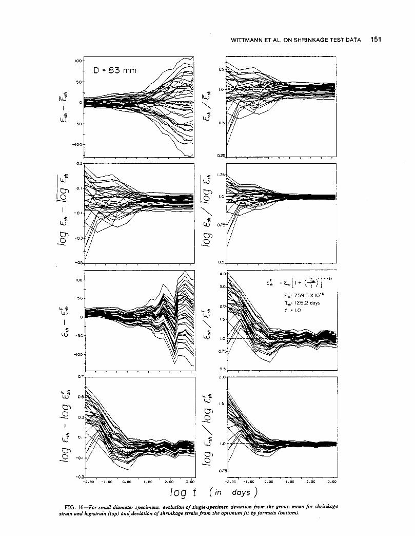
The evolution of statistical scatter in time is further illustrated in Figs_ 14, 16, 17. Figure 14 shows the history ofall specimens in one plot (that is, the plot of the values of f.h according to lines 1-36 of Tables 1 and 2). Figures 16 and 17 (for two specimen diameters D) show the evolution of the deviation from the group mean, for both f.h and log E.h, and for various types of mean (mean of E.h or log f.h

from all specimens used). On the bottom of Figs. 16-17, one can see the evolution of the deviations from the optimum fit by the for­mula (Eq 9).

... 2.00 0=160 mm 0- 0

O"l 1.95 t = 3 days

0

0 Y = 1.853

II 1.90 5L =0.077

-'= ",~,=0.0094 uJ

I.B5

O"l 0 0

LBO

II

>- 1.75

0 1.70

.£ 2 2.62 - t = 91 days 00

(J) Y =2.562 2.60

Q) 5L =0.032 O"l 2.58 w~=0.0036 0

....::s:::

.£ 2.56 L.

65 2.54

2.52 0

2.50 I 2 5 10 30 50 70 90

2.36

2.32

2.2B

2.24

2.20

2.B6

0

2.B4

2.B2

2.80

2.7B

2.76

95 9B 99 I

WITTMANN ET AL. ON SHRINKAGE TEST DATA

t = 21 days

Y =2.268 5L =0.043

0

t = 554 days

Y = 2.814 5L =0.026 w;,,=0.0031

. ~,., ..

0

0

0

2 5 10 30

. . . ....

50

0

00

0

70

0

0 0

0

90 95 9B 99

139

X = ( i - 0.375 )I(N +0.25) ( in %)

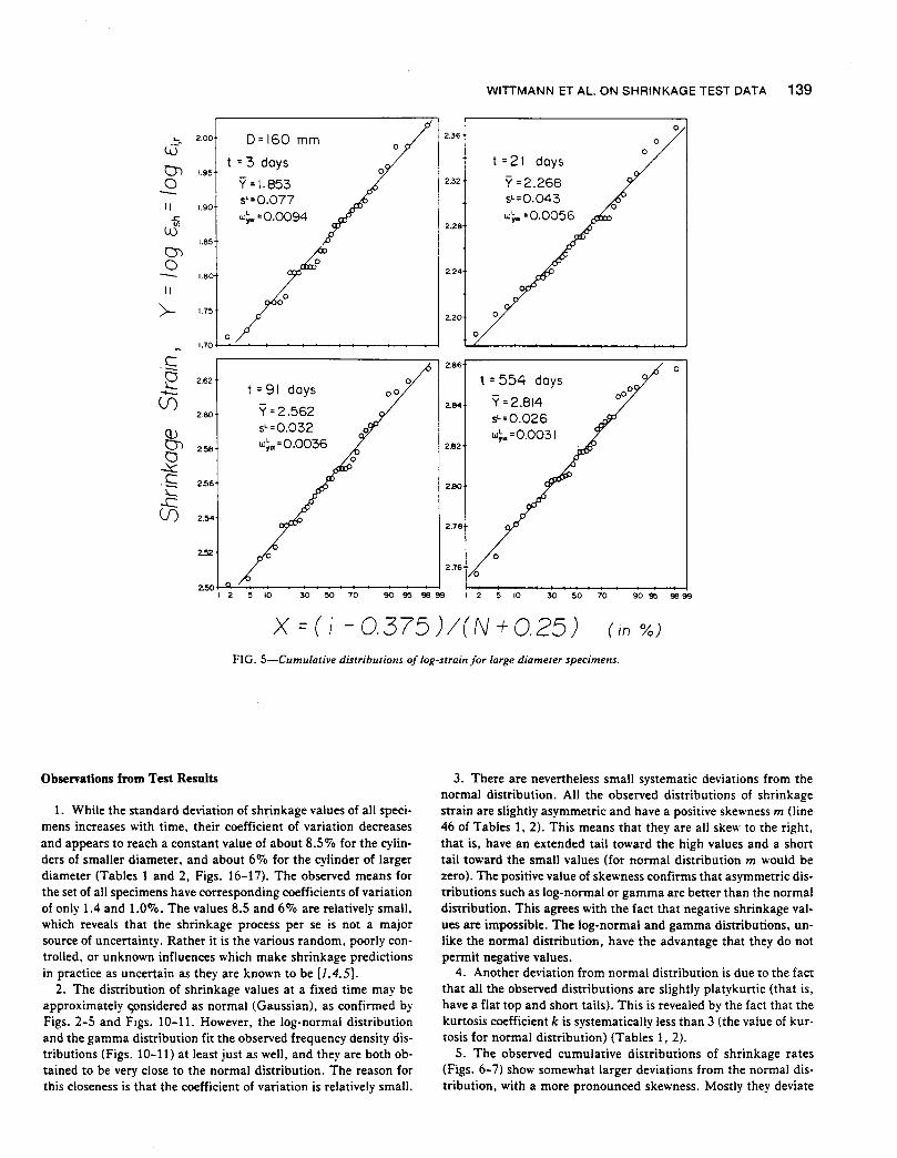
FIG. 5-Cumulative distributions of log-strain for large diameter specimens.

Observations from Test Results

1. While the standard deviation of shrinkage values of all speci­mens increases with time. their coefficient of variation decreases and appears to reach a constant value of about 8.50/0 for the cylin­ders of smaller diameter. and about 6% for the cylinder of larger diameter (Tables 1 and 2. Figs. 16-17). The observed means for the set of all specimens have corresponding coefficients of variation of only 1.4 and 1.0%. The values 8.5 and 6% are relatively small. which reveals that the shrinkage process per se is not a major source of uncertainty. Rather it is the various random. poorly con­trolled. or unknown influences which make shrinkage predictions in practice as uncertain as they are known to be [1.4.5].

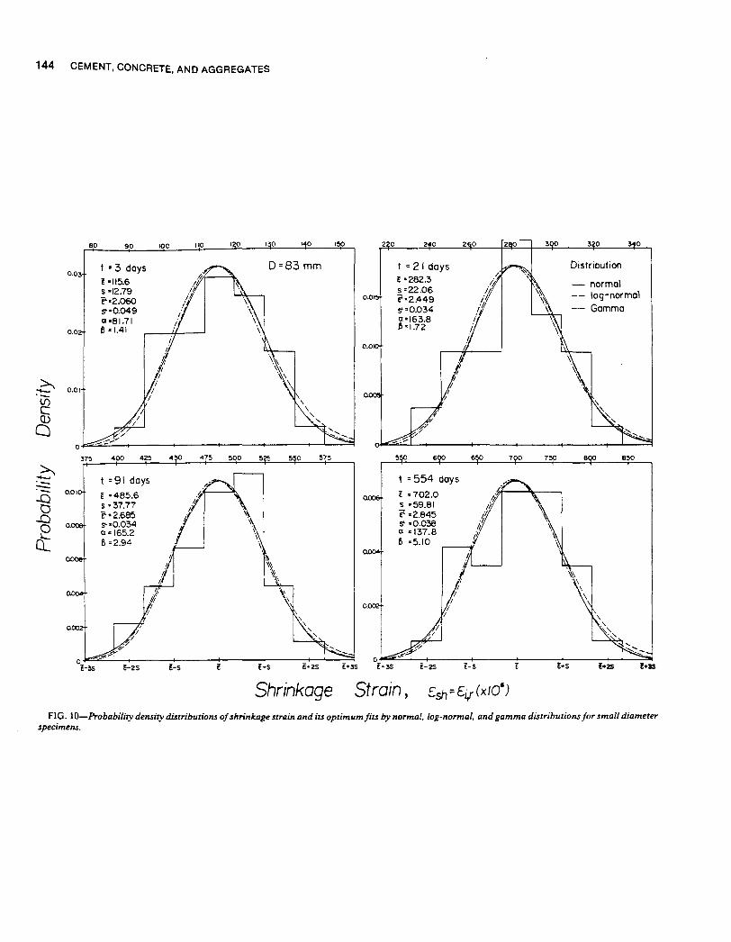
2. The distribution of shrinkage values at a fixed time may be approximately c;onsidered as normal (Gaussian). as confirmed by Figs. 2-5 and FIgs. 10-11. However, the log-normal distribution and the gamma distribution fit the observed frequency density dis­tributions (Figs. 10-11) at least just as well, and they are both ob­tained to be very close to the normal distribution. The reason for this closeness is that the coefficient of variation is relatively small.

3. There are nevertheless small systematic deviations from the normal distribution. All the observed distributions of shrinkage strain are slightly asymmetric and have a positive skewness m (line 46 of Tables 1, 2). This means that they are all skew to the right, that is, have an extended tail toward the high values and a short tail toward the stnall values (for normal distribution m would be zero). The positive value of skewness confirms that asymmetric dis­tributions such as log-normal or gamma are better than the normal distribution. This agrees with the fact that negative shrinkage val­ues are impossible. The log-normal and gamma distributions, un­like the normal distribution, have the advantage that they do not permit negative values.

4. Another deviation from normal distribution is due to the fact that all the observed distributions are slightly platykurtic (that is, have a flat top and short tails). This is revealed by the fact that the kurtosis coefficient k is systematically less than 3 (the value of kur­tosis for normal distribution) (Tables 1, 2).

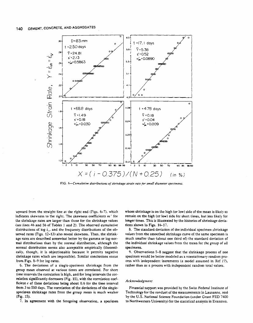
S. The observed cumulative distributions of shrinkage rates (Figs. 6-7) show somewhat larger deviations from the normal dis­tribution, with a more pronounced skewness. Mostly they deviate

140 CEMENT, CONCRETE, AND AGGREGATES

0 6.3 0

30 D=83mm t =17.1 days 0 0

t =2.50 days Y=5.38 5.9

28 Y =24.81 0

.~ s'=0.52 'W s'=2.13 w;"=0.0890

11 w;"=0.5863 5.5 .t:::. 26

·uS 11

>- 24 5.1

000

22 4.1

Q) 0 -+-

0 0 o 0 cr:: 20 4.3

.f; 0

0 1 =68.8 days 0.28 t =478 days '- I.e -c.n Y =1.49 Y =0.18

0 0 s'=0.18 0.24 s' =0.04

Q) w; .. =0.030 w;"=0.009 CJ\ 1.6 0 ~ 0.20 C '-'-tis 1.4

0.16

0 0

0 1.2 0 0.12 0

I 2 5 10 30 50 70 90 95 9899 I 2 5 10 30 50 70 90 95 9899

X = ( i - 0,375)I(N +0.25) ( in %)

FIG. 6-Cumulative distributions oj shrinkage strain ratejor small diameter specimens.

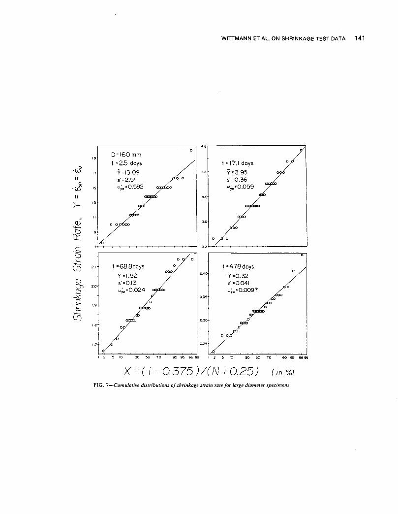
upward from the straight line at the right end (Figs. 6-7). which indicates skewness to the right. The skewness coefficients m' for the shrinkage rates are larger than those for the shrinkage values (see lines 46 and 56 of Tables 1 and 2). The observed cumulative distributions of log fi.r and the frequency distributions of the ob­served rates (Figs. 12-13) also reveal skewness. Thus, the shrink­age rates are described somewhat better by the gamma or log-nor­mal distributions than by the normal distribution, although the normal distribution seems also acceptable empirically (theoreti­cally, though, it is objectionable because it permits negative shrinkage rates which are impossible). Similar conclusions ensue from Figs. 8-9 for log-rates.

6. The deviations of a single-specimen shrinkage from the group mean observed at various times are correlated. For short time intervals the correlation is high, and for long intervals the cor­relation significantly decreases (Fig. 15), with the correlation coef­ficient c of these deviations being about 0.6 for the time interval from 3 to 550 days. The correlation of the deviations of the single­specimen shrinkage rates from the group mean is much weaker (Fig. 15).

7. In agreement with the foregoing observation, a specimen

whose shrinkage is on the high (or low) side of the mean is likely to remain on the high (or low) side for short times, but less likely for longer times. This is illustrated by the histories of shrinkage devia­tions shown in Figs. 16-17.

8. The standard deviation of the individual specimen shrinkage values from the smoothed shrinkage curve of the same specimen is much smaller than (about one third of) the standard deviation of the individual shrinkage values from the mean for the group of all specimens.

9. Observations 5-8 suggest that the shrinkage process of one specimen would be better modeled as a non stationary random pro­cess with independent increments (a model assumed in Ref 17), rather than as a process with independent random total values.

Acknowledgment

Financial support was provided by the Swiss Federal Institute of Technology for the conduct of the measurements in Lausanne, and by the U.S. National Science Foundation (under Grant FED 7400 to Northwestern University) for the statistical analysis in Evanston.

WITTMANN ET AL. ON SHRINKAGE TEST DATA 141

4.6 0

19 D=160mm

t =2.5 days t = 17.1 days 0

.~ 'W 17 9=13.09 4.4 9 =3.95 II 5'=2.51 00 5'=0.36 ~

w;"'=0.592 w;.=0.059 'L0 15

II 4.0

>- 13

" ~

CD 3.6 o 0 ........ 00

& 9

0 0 0

.f; 7 3.2

0 0

~ 0 0 - t =68.8days 0 t =478days en 2.1 000 0

9 =1.92 0.4 9 =0.32 CD 5'=0.13 5' =0.041 0> 2.0 0

0 w~.=0.024 w;,,=0.0097 ~ 0.35

.£; 0

~ 1.9

r--en 0.3 1.6

/ 1.7 0.25

3C 5C 70 9095 9S 99 I 2 5 10 30 50 70 9095 9899

X = ( i - 0.375 )I(N +0.25) ( in %)

FIG. 7-Cumulative distributions oj shrinkage strain ratejor large diameter specimens.

142 CEMENT, CONCRETE, AND AGGREGATES

WITIMANN ET AL. ON SHRINKAGE TEST DATA 143

0

0= 160 mm

t = 2.5 0 t = 17. I days 0 days 0

0.44 Y =0.398 '(=0.507

0 r¢} :;::I.~ 5'1.=0.037 VJ 5""=0.122

0 o~ II w:"=0.0261

w~.=0.0061 0

... .z:: 10

0.4

II 0

>-0.36

0 Q) -&

.f; 0

0

0 t =68.8 days o. t=478 days L. - Y =00411 Y =0.243 (f) 5'1.=0.033 0.26 s'''=0.024

Q) w~.=0.0133 w~.=0.0080 0 O'l 0

0 0.26

...::c 0

.f; 00 00

L. 0.24\ r-

C0 I

D.22t

0

O.3~ 2 I 5 10 30 5C 10 90 ~ 96 99 ~ I~ 30 5C 7';) 90 95 96 99

X ( i - 0.375 )I( N + 0.25) ( in %)

FIG. 9-Cumulative distributions oj the rate oj lag-strain jar large diameter specimens.

144

~ '--'-..Q CJ

..Q o ct

CEMENT, CONCRETE, AND AGGREGATES

eo 90 100 110 150 2 0 240

t = 3 days 0=83 mm t = 21 days 0.03

l-1I5.6 l =282.3 5 -12.79 5=22.06 ['=2.060 r=2.449 5"=0.049 5"=0.034 0-81.71 0=163.8

0.0 6 -1.41 6=1.72

0.01

o~~~~~-----+------~------+-----~--~~~

37~

t =91 days

E -485.6 5 =37.77 ['=2.685 5"=0.034 0= 165.2 B =2.94

e-2S los E·S

Shrinkage

l~3S

t = 554 days

E =702.0 s -59.81 (t -2.845 5" =0.038 0=137.8 6 =5.10

E-2S

Strain,

normal log-normal Gamma

e-s 1+35

FIG. lO-Probability density distributions of shrinkage strain and its optimumfiu by normal. log-normal. and gamma distributions for small diameter specimens.

WITIMANN ET AL. ON SHRINKAGE TEST DATA 145

40 50 60 70 9 10 1"0 160 240

0.0 t = 3 days D=160 mm t = 21 days

l - 72.3 E =186.4 - normal s -13.12 s -18.89 t' =1.853 t' =2.268 -- log-normal S' =0.0774 S' =0.0432 _.- Gamma a =30.42 0.015 a =97.40

0.02 6 =2.38 6 =1.91

.b "-If) c: 0.01 (l)

a o.

// .'/ /; . ..-:.. ....

.b 0

'- 300 330 360 560 600 640 680 720 760 -'-15 0.QI5 t =91 days t :554 days 0.010

~ l =365.7 l - 652.3 s -27.16 s = 38.35 t' -2.562 E' =2.814 '!if -0.0321 '!if =0.0259

0.010 a -181.4 a '289.4 6 =2.02 6 '2.25

o~~~--+-------+-------+-------~----~~~~~ !-2S !-s l+s f+2S t+s E-3S l-2S E-S l+s E+2S e+JS

SlTinkage Strain, FIG. II-Probability density distributions of shrinkage strain and its optimum fits by normal. log-normal. and gamma distributions for large diameter

specimens.

146 CEMENT, CONCRETE, AND AGGREGATES

It 21 2~ 27 2t 51 "'0 4~ ~.!\ • .0 .. ~ t =25 days 0= 83 mm t = 17.1 days Distri·bution £'. 24.607 t'· 5.3785 - normal

0.20 S· 2.1305 S· 0.5187 ('·1.393 ~. 0.7286 -- log-normal t;-·Q.03678

o.~ tr· 00427 -.- Gamma a.'. 135.57 a'· 107.53

0.15 fj • 0.183 Il'. 0.05

0.50

~ ....... 0.10 '-If) C Q)

a o.os

-C I.O~ 1.20 I.~ 1.50 1.6~ 1.&0 1.95 0.0. 0.12 0.15 OJ8 0.21 O~ 0.27 '--'-..Q t =68.8 days t =478 days CJ

..Q 2.50 E'· 1.4943 g'. 0.18435

0 5'· 0.178 '15= 0.0367

ct ~·0.1715 e-·-0.7423 S'" • 0.0El55 1000

1 ~. 0.08391

a' = 70.491 a'= 25.257 p; = 0.0212 fI' • 0.007299

7.50-'-

I ~.oo+

I

I 2.50+

I

o. (-25 i-s {·s {.2S l+3S {-5S ~-2S F,-s I ~.S E+2S E-tlS

Shrinkage Strain Rate, 85M =E:i,r (xlo6

)

FIG. 12-Probability density distributions oj shrinkage strain rate (Eq 2) jor small diameter specimens.

·-(J) c Q)

a

.--:..0 a

..Q o ct

0.20

O.I~

0.10 *"

3.00

'001

'001

t = 2.5 days

~'. 13.09 S'. 2.500 ~. 1.109 1· 0.0857 a'. 27.20 II' • 0.481

1.6 1.7

t =68.8days

t= 1.921 S'. 0.1298 t-. 0.2826 S'": 0.0292 0' • 219.04 B' : 0.00877

(-2S

"

I.e

Hi

WITTMANN ET AL. ON SHRINKAGE TEST DATA 147

13 I~ 17 " • 1.&0 r---+----+-----<,.....-F=~---+---...... ---__,

D .. 160 mm

1.20

0.80

0.&0

0.30

1.9 2.0 2.1

10.00

~.

1+15

Shrinkage Strain Rate,

t = 17.1 days

e· 3.95 S' 0.3610 t· 0.595 ~. 0.0398 rio 119.82 ri. 0.03298

0.21 0.24 0.27

t =478 days

t. 0.3166 S' 00435 t-·-0.5035 ~. 0.0604 a'= 52.87 II': 0.00599

{-2S {-$

0.:10 0.13

1

Distribution

- normal -- log-normal -.- Gamma

0.311 0.311 0.42

FIG. 13-Probabiliry de,u;'" d;.tributions of shrinkage strain rate for large diamev

148 CEMENT, CONCRETE, AND AGGREGATES

1 ~~~E 3-Normalized correlation moments jar individual specimens.

Shrinkage Strain Shrinkage Strain Rate

I, I. cr .q c!.q t, I. c:.q 'L clog cr .q '.q

0= 83MM

3 3 1.000 1.000 2.5 2.5 1.000 1.000 1.000 3 21 0.771 0.776 2.5 17.1 0.542 0.627 0.542 3 91 0.718 0.725 2.5 68.8 0.196 -0.153 0.201 3 554 0.679 0.689 2.5 477.8 0.535 -0.050 0.557 3 1399 0.671 0.681 2.5 880.4 0.207 0.337 0.190

21 21 1.000 1.000 17.1 17.1 1.000 1.000 1.000 21 91 0.959 0.961 17.1 68.8 0.190 -0.226 0.174 21 554 0.935 0.939 17.1 477.8 0.487 -0.065 0.530 21 1399 0.942 0.946 17.1 880.4 0.342 0.329 0.369 91 91 1.000 1.000 68.8 68.8 1.000 1.000 1.000 91 554 0.985 0.986 68.8 477.8 0.317 -0.191 0.318 91 1399 0.983 0.985 68.8 880.4 -0.472 -0.468 -0.457

554 554 1.000 1.000 477.8 477.8 1.000 1.000 1.000 554 1399 0.998 0.998 477.8 880.4 0.051 -0.068 0.040

1399 1399 1.000 1.000 880.4 880.4 1.000 1.000 1.000

0= 160MM 3 3 1.000 1.000 2.5 2.5 1.000 1.000 1.000 3 21 0.895 0.889 2.5 17.1 0.276 0.423 0.234 3 91 0.746 0.741 2.5 68.8 0.127 0.448 0.081 3 554 0.561 0.554 2.5 477.8 0.558 0.537 0.565 3 1399 0.561 0.554 2.5 880.4 0.426 0.213 0.409

21 21 1.000 1.000 17.1 17.1 1.000 1.000 1.000 21 91 0.950 0.950 17.1 68.8 0.656 0.592 0.656 21 554 0.842 0.843 17.1 477.8 0.671 0.395 0.647 21 1399 0.837 0.837 17.1 880.4 0.313 -0.003 0.324 91 91 1.000 1.000 68.8 68.8 1.000 1.000 1.000 91 554 0.950 0.948 68.8 477.8 0.235 -0.122 0.228 91 1399 0.941 0.939 68.8 880.4 0.311 0.084 0.331

554 554 1.000 1.000 477.8 477.8 1.000 1.000 1.000 554 1399 0.994 0.994 477.8 880.4 0.328 0.158 0.348

1399 1399 1.000 1.000 880.4 880.4 1.000 1.000 1.000

WIDMANN ET AL. ON SHRINKAGE TEST DATA 149

800 D = 83 mm D= 160mm Number of Measured Curves· 36 NlXIlber of Measured Curves' 35

700

10 0 600 -><

4:

L0' 500

.S;

~ 400 .... (f)

Q) 300 O"l 0 ~ .S;

200

~ 100

0 -2 -2 2

log t ( In days)

FIG. 14-Shrinkage strain versus log-time for all individual specimens.

TABLE 4-Standard deviations relative to optimum fit by formula.

o < t :s 1399 0<t:s90 90 < t :s 1399 6 :s t :s 1399

D=83MM

1.0 1.0 0.27 1.0 1.32 1.0 0.96 E~ 759.5 893.3 18776 767.5 742.4 759.3 765.8 .,. 126.2 179.6 60346 140.3 171.9 126.0 124.6

35.97 18.18 18.06 55.10 54.77 43.78 43.76 s* 12.50 6.72 6.72 15.91 15.91 13.98 13.98 SL 0.1187 0.1467 0.1325 0.0377 0.0377 0.0374 0.0374 s$L 0.1153 0.1:!28 0.1228 0.0123 0.0123 0.0122 0.0122 s*/s 0.3476 0.3093 0.3718 0.2888 0.2905 0.3193 0.3194 S$L/SL 0.9711 0.8369 0.9265 0.3270 0.3273 0.3255 0.3258 I 34.89 17.43 17.28 54.74 54.40 42.96 42.94 Sis 0.9701 0.9586 0.9567 0.9934 0.9933 0.9813 0.9813 W 0.2944 0.3893 0.3655 0.2911 0.2900 0.2876 0.2871

D = 160MM r 1.0 1.0 0.21 1.0 2.08 1.0 1.49 E~ 771.2 841.6 127360 762.8 687.7 771.5 707.2 .,. 306.3 388.7 6885373 284.9 343.6 306.9 305.8

26.75 15.54 15.39 39.61 36.42 32.06 30.40 s* 11.43 10.36 10.36 13.67 13.67 12.22 12.22 SL 0.1285 0.1629 0.1496 0.0308 0.0290 0.0408 0.0396 s$L 0.1333 0.1325 0.1325 0.0130 0.0130 0.0160 0.0160 s*/s 0.4272 0.6663 0.6729 0.3450 0.3752 0.3812 0.4019 S$L/SL 1.0375 0.8138 0.8857 0.4211 0.4473 0.3916 0.4030 I 25.28 14.77 14.63 39.31 35.44 31.03 29.13 Sis 0.9452 0.9502 0.9508 0.9923 0.9731 0.9680 0.9582 W 0.3232 0.4644 0.4416 0.2671 0.2521 0.2975 0.2870

150 CEMENT, CONCRETE, AND AGGREGATES

(j) -+---C Q)

E o 2 c o

-+--o -Q) L L o

U

\J Q)

.~ -E <s z

.771 .718

D83mm 0.5OI----+------+-----+-'

tr ...J~'"

1.00

UO.7

0.5

1.0

tr , ~ ... 0.5 U

0.0

1.0

0.5

0.0

~6 .961 . 39

.77 .725 . 9

-Cl.226

-0.5+-------~--------~~----~

1.0

0.0

o

..... !557 " , 'f~:30 . \/ ''0 ~8

\ " .174 \ \

2

log t

1

o

D 160mm

43

.741

.554

r , \

--q----<? r \ \ ~ \ \ /. '. \. ~.\f". >."\ .&47

\ .~~~ \ ~ ·565 ./ i.4'

V .

2

(In doys)

FIG. IS-Correlarion between shrinkage values at various times.

WITTMANN ET AL. ON SHRINKAGE TEST DATA 151

100

D = 83 mm ~o

..r:.

uS

uJ

~ en 0 -

"" ..r:. ..r:. ~r '" lU

en en 0 0 - -

100 E;. [ Cr. ),]""" = E ... 1+ T

~o E ... : 759.5 X 10-6

L..,: 126.2 days ... .c r • 1.0 uS lJ 0

I

"" .c

uS .c -~o uS

-100

0.7

... .:: ll,.r ... .::

lU'" en en 0 - 0 -

..r:.

"" uS ..r:.

uS en 0 en - 0 -

-2.00 -1.00 0.00 1.00 J.OO -2.00 -1.00 0.00 1.00 2.00 J.OO

log t ( in days)

FIG. 16-For small diameter specimens. evolution of single-specimen deviation from the group mean for shrinkage strain and log-strain (top) and. deviation of shrinkage strain from the optimum fit by formula (bottom).

152 CEMENT, CONCRETE, AND AGGREGATES

2.0~--------------------------------~

0= 160 mm

..0::: ..0:::

'" L0 lU

en 0 -

..0::: ..0:::

L0 L0

-0.5

100 -'

E~h = E 1+ ~ [ Cr. )'] -112. GO t

50 £.. = 771.2 X 10'"

.... iii 7 •• = 306.3 days

lU r = 1.0

0 ~ ..0::: ..0:::

uS uS -50

-100

... ..0:::

lU'" ... ..0:::

lU"'

en en 0 0 - -

~ ..0::: ..0:::

lU'" lJ' en 0 -

.00 -1.00 O. 1.00 2.00 J.OO

log t ( in days) FIG. 17-For. large diameter specimens. evolution of single-specimen deviation from the group mean for shrinkage

strain and log-strain (top) and deviation of shrinkage strain from the optimum fit by formula (bottom).

References

(1) Tsubaki. T. et al.. "Probabilistic Models." Chapter 5 of State-of-Art Report by RILEM Committee TC69 chaired by Z. P. Bazant. Pre­prints. Fourth RILEM International Symposium on Creep and Shrinkage of Concrete: Mathematical Modeling, Z. P. Bazant, Ed., Northwestern University. Evanston. IL, Aug. 1986, pp. 383-454 (pre­print volume available from Northwestern University).

(2) Madsen, H. O. and Baiant, Z. P., "Uncertainty Analysis of Creep and Shrinkage Effects in Concrete Structures," ACI Journal. Vol. 80, Mar.-Apr. 1983, pp. 116-127.

(3) Bazant. Z. P. and Liu. K. L., "Random Creep and Shrinkage in Structures," Journal oj Structural Engineering. ASCE, Vol. 111, 1985. pp. 113-134.

(4) Bazant, Z. P. and Panula. L., "Practical Prediction of Time-Depen­dent Deformations of Concrete," Materials and Structures. Parts I and II: Vol. 11. No. 65.1978. pp. 307-328; Parts III and IV: Vol. 11. No. 66.1978. pp. 415-434; Parts V and VI: Vol. 12, No. 69,1979, pp. 169-183.

(5) Bazant, Z. P. and Panula, L., "Creep and Shrinkage Characteriza­tion for Analyzing Prestressed Concrete Structures," Prestressed Con­crete Institute. Journal. Vol. 25. No.3, 1980, pp. 86-122.

(6) Bazant, Z. P. and Panula, L., "New Models for Practical Prediction of Creep and Shrinkage." in Designing jor Creep and Shrinkage in Concrete Structures. (Proceedings of A. Pau\\' Symposium held in Houston, 1978), ACI Special Publication SP-76. American Concrete Institute. Detroit, 1982, pp. 7-23.

(7) Alou. F. and Wittmann. F. H .• "Etude experimentale de la variabilite du retrait du beton." Proceedings, International Symposium on Fun­damental Research on Creep and Shrinkage of Concrete. Lausanne, Sept. 1980, F. H. Wittmann, Ed., Martinus Nijhoff, Netherlands 1982, pp. 75-92.

(8) Reinhardt, H. W., Pat, M. G. M., and Wittmann, F. H., "Variability of Creep and Shrinkage of Concrete," Proceedings, International Symposium on Fundamental Research on Creep and Shrinkage of

WITIMANN ET AL. ON SHRINKAGE TEST DATA 153

Concrete, Lausanne, Sept. 1980, F. H. Wittmann, Ed., Martinus Nij­hoff. Netherlands, 1982, pp. 95-108.

(9) Cornelissen. H., "Creep of Concrete-A Stochastic Quantity." Ph.D. thesis, Technical University. Eindhoven, The Netherlands, 1979 (in Dutch. with extended English summary).

(10) Cornelissen, H., "Creep of Concrete-A Stochastic Quantity," Pro­ceedings, International Symposium on Fundamental Research on Creep and Shrinkage of Concretes. Lausanne, Sept. 1980, Martinus Nijhoff, Netherlands 1982, pp. 109-124.

(II) Buant. Z. P .• "Statistics of Shrinkage Test Data: Formulation and Method," Internal Report, Cooperative Project NU-EPFL, North­western University, Evanston, IL, May 1985.

(12) Bazant, Z. P., Wittmann, F. H., Kim, J.-K., and Alou, F .• "Statisti­cal Extrapolation of Shrinkage Data-Part I: Regression," ACI Ma­terialsJournal. Vol. 34. Jan.-Feb. 1987, pp. 20-34.

(131 Bazant. Z. P., Kim, J.-K., Wittmann, F. H., and Alou, F., "Statisti­cal Extrapolation of Shrinkage Data-Part II: Bayesian Updating," ACI Materials Journal. Vol. 84, Mar.-Apr. 1987, pp. 83-91.

(14) Bulmer, M. G., Principles oj Statistics. Dover Publications, New York,1979.

(15) Benjamin, J. R. and Cornell, A. C., Probability. Statistics and Deci­sionjor Civil Engineers, McGraw-Hili, New York, 1970.

(16) Blom, G., "Statistical Estimates and Transformed Data Variables," Ch. 12,1. Wiley, New York, 1958.

(17] Cinlar, E., Baiant, Z. P., and Osman, E., "Stochastic Process for Extrapolating Concrete Creep," Journal oj the Engineering Mechan­ics Division. Proceedings of the American Society of Civil Engineers, New York, Vol. 103, 1977, pp. 1069-1088; Discussion 1979, pp. 485-489.

(18) Miller, I. and Freund, J., Probability and Statistics jor Engineers. Prentice Hall, Englewood Cliffs, NJ, 1965, pp. 78-80.

(19) Kimball, B. F., "On the Choice of Plotting Positions on Probability Paper," Journal oj the American Statistical Association. Vol. 55, No. 291, Sept. 1960, pp. 546-560.

(20) Martz, H. F. and Waller, R. A., Bayesian Reliability Analysis. J. Wi­ley, New York, 1982, p. 115.