statistical regression analysisusers.stat.ufl.edu/~winner/sta6208/allreg5.pdfstatistical regression...
TRANSCRIPT

Statistical Regression Analysis
Larry Winner
University of Florida
Department of Statistics
August 15, 2017

2

Contents
1 Probability Distributions, Estimation, and Testing 7
1.1 Introduction . . . . . . . . . . . . . . . . . . . . . . . . . . . . . . . . . . . . . . . . . . . . . . 7
1.1.1 Discrete Random Variables/Probability Distributions . . . . . . . . . . . . . . . . . . 7
1.1.2 Continuous Random Variables/Probability Distributions . . . . . . . . . . . . . . . . . 10
1.2 Linear Functions of Multiple Random Variables . . . . . . . . . . . . . . . . . . . . . . . . . . 15
1.3 Functions of Normal Random Variables . . . . . . . . . . . . . . . . . . . . . . . . . . . . . . 17
1.4 Likelihood Functions and Maximum Likelihood Estimation . . . . . . . . . . . . . . . . . . . 21
1.5 Likelihood Ratio, Wald, and Score (Lagrange Multiplier) Tests . . . . . . . . . . . . . . . . . 35
1.5.1 Single Parameter Models . . . . . . . . . . . . . . . . . . . . . . . . . . . . . . . . . . 36
1.5.2 Multiple Parameter Models . . . . . . . . . . . . . . . . . . . . . . . . . . . . . . . . . 39
1.6 Sampling Distributions and an Introduction to the Bootstrap . . . . . . . . . . . . . . . . . . 42
2 Simple Linear Regression - Scalar Form 47
2.1 Introduction . . . . . . . . . . . . . . . . . . . . . . . . . . . . . . . . . . . . . . . . . . . . . . 47
2.2 Inference Regarding β1 . . . . . . . . . . . . . . . . . . . . . . . . . . . . . . . . . . . . . . . . 55
2.3 Estimating a Mean and Predicting a New Observation @ X = X∗ . . . . . . . . . . . . . . . 57
2.4 Analysis of Variance . . . . . . . . . . . . . . . . . . . . . . . . . . . . . . . . . . . . . . . . . 59
2.5 Correlation . . . . . . . . . . . . . . . . . . . . . . . . . . . . . . . . . . . . . . . . . . . . . . 64
3

4 CONTENTS
2.6 Regression Through the Origin . . . . . . . . . . . . . . . . . . . . . . . . . . . . . . . . . . . 67
2.7 R Programs and Output Based on lm Function . . . . . . . . . . . . . . . . . . . . . . . . . . 71
2.7.1 Carpet Aging Analysis . . . . . . . . . . . . . . . . . . . . . . . . . . . . . . . . . . . . 71
2.7.2 Suntan Product SPF Assessments . . . . . . . . . . . . . . . . . . . . . . . . . . . . . 74
3 Simple Linear Regression - Matrix Form 77
4 Distributional Results 85
5 Model Diagnostics and Influence Measures 93
5.1 Checking Linearity . . . . . . . . . . . . . . . . . . . . . . . . . . . . . . . . . . . . . . . . . . 93
5.2 Checking Normality . . . . . . . . . . . . . . . . . . . . . . . . . . . . . . . . . . . . . . . . . 99
5.3 Checking Equal Variance . . . . . . . . . . . . . . . . . . . . . . . . . . . . . . . . . . . . . . 105
5.4 Checking Independence . . . . . . . . . . . . . . . . . . . . . . . . . . . . . . . . . . . . . . . 108
5.5 Detecting Outliers and Influential Observations . . . . . . . . . . . . . . . . . . . . . . . . . . 110
6 Multiple Linear Regression 119
6.1 Testing and Estimation for Partial Regression Coefficients . . . . . . . . . . . . . . . . . . . . 120
6.2 Analysis of Variance . . . . . . . . . . . . . . . . . . . . . . . . . . . . . . . . . . . . . . . . . 120
6.3 Testing a Subset of βs = 0 . . . . . . . . . . . . . . . . . . . . . . . . . . . . . . . . . . . . . . 122
6.4 Tests Based on the Matrix Form of Multiple Regression Model . . . . . . . . . . . . . . . . . 122
6.4.1 Equivalence of Complete/Reduced Model and Matrix Based Test . . . . . . . . . . . . 124
6.4.2 R-Notation for Sums of Squares . . . . . . . . . . . . . . . . . . . . . . . . . . . . . . 131
6.4.3 Coefficients of Partial Determination . . . . . . . . . . . . . . . . . . . . . . . . . . . . 135
6.5 Models With Categorical (Qualitative) Predictors . . . . . . . . . . . . . . . . . . . . . . . . . 136
6.6 Models With Interaction Terms . . . . . . . . . . . . . . . . . . . . . . . . . . . . . . . . . . . 140

CONTENTS 5
6.7 Models With Curvature . . . . . . . . . . . . . . . . . . . . . . . . . . . . . . . . . . . . . . . 144
6.8 Response Surfaces . . . . . . . . . . . . . . . . . . . . . . . . . . . . . . . . . . . . . . . . . . 148
6.9 Trigonometric Models . . . . . . . . . . . . . . . . . . . . . . . . . . . . . . . . . . . . . . . . 153
6.10 Model Building . . . . . . . . . . . . . . . . . . . . . . . . . . . . . . . . . . . . . . . . . . . . 156
6.10.1 Backward Elimination . . . . . . . . . . . . . . . . . . . . . . . . . . . . . . . . . . . . 158
6.10.2 Forward Selection . . . . . . . . . . . . . . . . . . . . . . . . . . . . . . . . . . . . . . 159
6.10.3 Stepwise Regression . . . . . . . . . . . . . . . . . . . . . . . . . . . . . . . . . . . . . 161
6.10.4 All Possible Regressions . . . . . . . . . . . . . . . . . . . . . . . . . . . . . . . . . . . 162
6.11 Issues of Collinearity . . . . . . . . . . . . . . . . . . . . . . . . . . . . . . . . . . . . . . . . . 163
6.11.1 Principal Components Regression . . . . . . . . . . . . . . . . . . . . . . . . . . . . . . 164
6.11.2 Ridge Regression . . . . . . . . . . . . . . . . . . . . . . . . . . . . . . . . . . . . . . . 169
6.12 Models with Unequal Variances (Heteroskedasticity) . . . . . . . . . . . . . . . . . . . . . . . 175
6.12.1 Estimated Weighted Least Squares . . . . . . . . . . . . . . . . . . . . . . . . . . . . . 180
6.12.2 Bootstrap Methods When Distribution of Errors is Unknown . . . . . . . . . . . . . . 191
6.13 Generalized Least Squares for Correlated Errors . . . . . . . . . . . . . . . . . . . . . . . . . . 196
7 Nonlinear Regression 205
8 Random Coefficient Regression Models 225
8.1 Balanced Model with 1 Predictor . . . . . . . . . . . . . . . . . . . . . . . . . . . . . . . . . . 225
8.2 General Model with p Predictors . . . . . . . . . . . . . . . . . . . . . . . . . . . . . . . . . . 226
8.2.1 Unequal Sample Sizes Within Subjects . . . . . . . . . . . . . . . . . . . . . . . . . . . 230
8.2.2 Tests Regarding Elements of Σβ . . . . . . . . . . . . . . . . . . . . . . . . . . . . . . 236
8.2.3 Tests Regarding β . . . . . . . . . . . . . . . . . . . . . . . . . . . . . . . . . . . . . . 240
8.2.4 Correlated Errors . . . . . . . . . . . . . . . . . . . . . . . . . . . . . . . . . . . . . . . 242

6 CONTENTS
8.3 Nonlinear Models . . . . . . . . . . . . . . . . . . . . . . . . . . . . . . . . . . . . . . . . . . . 242
9 Alternative Regression Models 249
9.1 Introduction . . . . . . . . . . . . . . . . . . . . . . . . . . . . . . . . . . . . . . . . . . . . . . 249
9.2 Binary Responses - Logistic Regression . . . . . . . . . . . . . . . . . . . . . . . . . . . . . . . 249
9.2.1 Interpreting the Slope Coefficients . . . . . . . . . . . . . . . . . . . . . . . . . . . . . 251
9.2.2 Inferences for the Regression Parameters . . . . . . . . . . . . . . . . . . . . . . . . . . 252
9.2.3 Goodness of Fit Tests and Measures . . . . . . . . . . . . . . . . . . . . . . . . . . . . 253
9.3 Count Data - Poisson and Negative Binomial Regression . . . . . . . . . . . . . . . . . . . . . 261
9.3.1 Poisson Regression . . . . . . . . . . . . . . . . . . . . . . . . . . . . . . . . . . . . . . 261
9.3.2 Goodness of Fit Tests . . . . . . . . . . . . . . . . . . . . . . . . . . . . . . . . . . . . 264
9.3.3 Overdispersion . . . . . . . . . . . . . . . . . . . . . . . . . . . . . . . . . . . . . . . . 268
9.3.4 Models with Varying Exposures . . . . . . . . . . . . . . . . . . . . . . . . . . . . . . . 271
9.4 Negative Binomial Regression . . . . . . . . . . . . . . . . . . . . . . . . . . . . . . . . . . . . 274
9.5 Gamma Regression . . . . . . . . . . . . . . . . . . . . . . . . . . . . . . . . . . . . . . . . . . 282
9.5.1 Estimating Model Parameters . . . . . . . . . . . . . . . . . . . . . . . . . . . . . . . . 283
9.5.2 Inferences for Model Parameters and Goodness of Fit Test . . . . . . . . . . . . . . . . 286
9.6 Beta Regression . . . . . . . . . . . . . . . . . . . . . . . . . . . . . . . . . . . . . . . . . . . . 293
9.6.1 Estimating Model Parameters . . . . . . . . . . . . . . . . . . . . . . . . . . . . . . . . 294
9.6.2 Diagnostics and Influence Measures . . . . . . . . . . . . . . . . . . . . . . . . . . . . 297

Chapter 1
Probability Distributions, Estimation,and Testing
1.1 Introduction
Here we introduce probability distributions, and basic estimation/testing methods. Random variables areoutcomes of an experiment or data-generating process, where the outcome is not known in advance, althoughthe set of possible outcomes is. Random variables can be discrete or continuous. Discrete random variablescan take on only a finite or countably infinite set of possible outcomes. Continuous random variables cantake on values along a continuum. In many cases, variables of one type may be treated as or reported as theother type. In the introduction, we will use upper-case letters (such as Y ) to represent random variables,and lower-case letters (such as y) to represent specific outcomes. Not all (particularly applied statistics)books follow this convention.
1.1.1 Discrete Random Variables/Probability Distributions
In many applications, the result of the data-generating process is the count of a number of events of somesort. In some cases, a certain number of trials are conducted, and the outcome of each trial is observed as a“Success” or “Failure” (binary outcomes). In these cases, the number of trials ending in Success is observed.Alternatively, a series of trials may be conducted until a pre-selected number of Successes are observed. Inother settings, the number of events of interest may be counted in a fixed amount of time or space, withoutactually breaking the domain into a set of distinct trials.
For discrete random variables, we will use p(y) to represent the probability that the random variable Ytakes on the value y. We require that all such probabilities be bounded between 0 and 1 (inclusive), andthat they sum to 1:
P Y = y = p(y) 0 ≤ p(y) ≤ 1∑
y
p(y) = 1
7

8 CHAPTER 1. PROBABILITY DISTRIBUTIONS, ESTIMATION, AND TESTING
The cumulative distribution function is the probability that a random variable takes on a value lessthan or equal to a specific value y∗. It is an increasing function that begins at 0 and increases to 1, andwe will denote it as F (y∗). For discrete random variables it is a step function, taking a step at each pointwhere p(y) > 0:
F (y∗) = P (Y ≤ y∗) =∑
y≤y∗
p(y)
The mean or Expected Value (µ) of a random variable is it’s long-run average if the experiment wasconducted repeatedly ad infinitum. The variance
(
σ2)
is the average squared difference between the randomvariable and its mean, measuring the dispersion within the distribution. The standard deviation (σ) isthe positive square root of the variance, and is in the same units as the data.
µY = E Y =∑
y
yp(y) σ2Y = V Y = E
(Y − µY )2
=∑
y
(y − µY )2p(y) σY = +
√
σ2Y
Note that for any function of Y , the expected value and variance of the function is computed as follows:
E g(Y ) =∑
y
g(y)p(y) = µg(Y ) V g(Y ) = E
(
g(Y ) − µg(Y )
)2
=∑
y
(
g(y) − µg(Y )
)2p(y)
For any constants a and b, we have the mean and variance of the linear function a+ bY :
E a+ bY =∑
y
ap(y) +∑
y
byp(y) = a∑
y
p(y) + b∑
y
yp(y) = a(1) + bE Y = a + bµY
V a+ bY =∑
y
((a + by) − (a+ bµY ))2 p(y) = b2∑
y
(y − µY )2 p(y) = b2σ2Y
A very useful result in mathematical statistics is the following:
σ2Y = V Y = E
(Y − µY )2
= E
Y 2 − 2µY Y + µ2
= E
Y 2
− 2µYE Y + µ2Y = E
Y 2
− µ2Y
Thus, E
Y 2
= σ2Y + µ2
Y . Also, from this result we obtain: E Y (Y − 1) = σ2Y + µ2
Y − µY . From this, wecan obtain σ2
Y = E Y (Y − 1) − µ2Y + µY , which is useful for some discrete probability distributions.
Next, we consider several families of discrete probability distributions: the Binomial, Poisson, andNegative Binomial families.
Binomial Distribution
When an experiment consists of n independent trials, each of which can end in one of two outcomes: Successor Failure with constant probability of success, we refer to this as a binomial experiment. The randomvariable Y is the number of Successes in the n trials, and can take on the values y = 0, 1, . . . , n. Note that insome settings, the “Success” can be a negative attribute. We denote the probability of success as π, whichlies between 0 and 1. We use the notation: Y ∼ B (n, π). The probability distribution, mean and varianceof Y depend on the sample size n and probability of success π.
p(y) =
(
n
y
)
πy (1 − π)n−y
E Y = µY = nπ V Y = σ2Y = nπ (1 − π)

1.1. INTRODUCTION 9
where(
ny
)
= n!y!(n−y)! . In practice, π will be unknown, and estimated from sample data. Note that to obtain
the mean and variance, we have:
E Y = µY =
n∑
y=0
yp(y) =
n∑
y=0
yn!
y!(n − y)!πy (1 − π)
n−y=
n∑
y=1
yn!
y!(n − y)!πy (1 − π)
n−y=
= nπ
n∑
y=1
(n− 1)!
(y − 1)!(n− y)!πy−1 (1 − π)
n−y= nπ
n−1∑
y∗=0
(
n− 1
y∗
)
πy∗
(1 − π)n−1−y∗
= nπ∑
y∗
p (y∗) = nπ y∗ = y−1
To obtain the variance, we use the result from above, σ2Y = E Y (Y − 1) − µ2
Y + µY :
E Y (Y − 1) =
n∑
y=0
y(y−1)p(y) =
n∑
y=0
y(y−1)n!
y!(n − y)!πy (1 − π)
n−y=
n∑
y=2
y(y−1)n!
y!(n − y)!πy (1 − π)
n−y=
= n(n− 1)π2n∑
y=2
(n− 2)!
(y − 2)!(n− y)!πy−2 (1 − π)
n−y= n(n− 1)π2
n−2∑
y∗∗=0
(
n − 2
y∗∗
)
πy∗∗
(1 − π)n−2−y∗∗
n(n− 1)π2∑
y∗∗
p (y∗∗) = n(n− 1)π2 y∗∗ = y − 2
⇒ σ2Y = n(n− 1)π2 − n2π2 + nπ = nπ − nπ2 = nπ (1 − π)
Poisson Distribution
In many applications, researchers observe the counts of a random process in some fixed amount of time orspace. The random variable Y is a count that can take on any non-negative integer. One important aspectof the Poisson family is that the mean and variance are the same. This is one aspect that does not work forall applications. We use the notation: Y ∼ Poi(λ). The probability distribution, mean and variance of Yare:
p(y) =e−λλy
y!E Y = µY = λ V Y = σ2
Y = λ
Note that λ > 0. The Poisson arises by dividing the time/space into n infinitely small areas, each havingeither 0 or 1 Success, with Success probability π = λ/n. Then Y is the number of areas having a success.
p(y) =n!
y!(n − y)!
(
λ
n
)y (
1 − λ
n
)n−y
=n(n− 1) · · · (n− y + 1)
y!
(
λ
n
)y (
1 − λ
n
)n−y
=
=1
y!
(n
n
)
(
n− 1
n
)
· · ·(
n− y + 1
n
)
λy
(
1 − λ
n
)n(
1 − λ
n
)−y
The limit as n goes to ∞ is:
limn→∞
p(y) =1
y!(1)(1) · · · (1)λye−λ(1) = p(y) =
e−λλy
y!
To obtain the mean of Y for the Poisson distribution, we have:
E Y = µY =∞∑
y=0
yp(y) =∞∑
y=0
ye−λλy
y!=
∞∑
y=1
ye−λλy
y!=
∞∑
y=1
e−λλy
(y − 1)!=

10 CHAPTER 1. PROBABILITY DISTRIBUTIONS, ESTIMATION, AND TESTING
λ
∞∑
y=1
e−λλ(y−1)
(y − 1)!= λ
∞∑
y∗=0
e−λλy∗
y∗!= λ
∑
y∗
p (y∗) = λ
We use the same result as that for the binomial to obtain the variance for the Poisson distribution:
E Y (Y − 1) =∞∑
y=0
y(y−1)p(y) =∞∑
y=0
y(y−1)e−λλy
y!=
∞∑
y=2
y(y−1)e−λλy
y!= λ2
∞∑
y=2
e−λλ(y−2)
(y − 2)!= λ2
∞∑
y∗∗=0
e−λλy∗∗
y∗∗!= λ2
⇒ σ2Y = λ2 − λ2 + λ = λ
Negative Binomial Distribution
The negative binomial distribution is used in two quite different contexts. The first is where a binomialtype experiment is being conducted, except instead of having a fixed number of trials, the experiment iscompleted when the rth success occurs. The random variable Y is the number of trials needed until the rth
success, and can take on any integer value greater than or equal to r. The probability distribution, its meanand variance are:
p(y) =
(
y − 1
r − 1
)
πr (1 − π)y − r E Y = µY =
r
πV Y = σ2
Y =r (1 − π)
π2.
A second use of the negative binomial distribution is as a model for count data. It arises from a mixtureof Poisson models. In this setting it has 2 parameters and is more flexible than the Poisson (which has thevariance equal to the mean), and can take on any non-negative integer value. In this form, the negativebinomial distribution and its mean and variance can be written as (see e.g. Agresti (2002) and Cameronand Trivedi (2005)).
f (y;µ, α) =Γ(
α−1 + y)
Γ (α−1) Γ (y + 1)
(
α−1
α−1 + µ
)α−1(
µ
α−1 + µ
)y
Γ(w) =
∫ ∞
0
xw−1e−xdx = (w − 1)Γ (w − 1) .
The mean and variance of this form of the Negative Binomial distribution are
E Y = µ V Y = µ (1 + αµ) .
1.1.2 Continuous Random Variables/Probability Distributions
Random variables that can take on any value along a continuum are continuous. Here, we consider thenormal, gamma, t, and F families. Special cases of the gamma family include the exponential and chi-squareddistributions. Continuous distributions are density functions, as opposed to probability mass functions. Theirdensity is always non-negative, and integrates to 1. We will use the notation f(y) for density functions. Themean and variance for continuous distributions are obtained in a similar manner as discrete distributions,with integration replacing summation.
E Y = µY =
∫ ∞
−∞
yf(y)dy V Y = σ2Y =
∫ ∞
−∞
(y − µY )2f(y)dy
In general, for any function g(Y ), we have:
E g(Y ) =
∫ ∞
−∞
g(y)f(y)dy = µg(Y ) V g(Y ) = E
(
g(Y ) − µg(Y )
)2
=
∫ ∞
−∞
(
g(y) − µg(Y )
)2f(y)dy

1.1. INTRODUCTION 11
Normal Distribution
The normal distributions, also known as the Gaussian distributions, are a family of symmetric mound-shaped distributions. The distribution has 2 parameters: the mean µ and the variance σ2, although oftenit is indexed by its standard deviation σ. We use the notation Y ∼ N
(
µ, σ2)
. The probability densityfunction, the mean and variance are:
f(y) =1√
2πσ2exp
(
−(y − µ)2
2σ2
)
E Y = µY = µ V Y = σ2Y = σ2
The mean µ defines the center (median and mode) of the distribution, and the standard deviation σ is ameasure of the spread (µ − σ and µ + σ are the inflection points). Despite the differences in location andspread of the different distributions in the normal family, probabilities with respect to standard deviationsfrom the mean are the same for all normal distributions. For −∞ < z1 < z2 <∞, we have:
P (µ+ z1σ ≤ Y ≤ µ+ z2σ) =
∫ µ+z2σ
µ+z1σ
1√2πσ2
exp
(
−(y − µ)2
2σ2
)
dy =
∫ z2
z1
1√2πe−z2/2dz = Φ(z2) − Φ(z1)
Where Z is standard normal, a normal distribution with mean 0, and variance (standard deviation) 1.Here Φ(z∗) is the cumulative distribution function of the standard normal distribution, up to the point z∗:
Φ(z∗) =
∫ z∗
−∞
1√2πe−z2/2dz
These probabilities and critical values can be obtained directly or indirectly from standard tables, statisticalsoftware, or spreadsheets. Note that:
Y ∼ N(
µ, σ2)
⇒ Z =Y − µ
σ∼ N(0, 1)
This makes it possible to use the standard normal table for any normal distribution. Plots of three normaldistributions are given in Figure 1.1.
Gamma Distribution
The gamma family of distributions are used to model non-negative random variables that are often right-skewed. There are two widely used parameterizations. The first given here is in terms of shape and scale
parameters:
f(y) =1
Γ(α)βαyα−1e−y/β y ≥ 0, α > 0, β > 0 E Y = µY = αβ V Y = σ2
Y = αβ2
Here, Γ(α) is the gamma function Γ(α) =∫∞
0yα−1e−ydy and is built-in to virtually all statistical packages
and spreadsheets. It also has two simple properties:
α > 1 : Γ(α) = (α− 1)Γ(α− 1) Γ
(
1
2
)
=√π.
Thus, if α is an integer, Γ(α) = (α− 1)!. The second version given here is in terms of shape and rate
parameters.
f(y) =θα
Γ(α)yα−1e−yθ y ≥ 0, α > 0, θ > 0 E Y = µY =
α
θV Y = σ2
Y =α
θ2

12 CHAPTER 1. PROBABILITY DISTRIBUTIONS, ESTIMATION, AND TESTING
0 20 40 60 80 100
0.0
00.0
50.1
00.1
5
Normal(µ,σ)
y
f(y)
N(25,5)
N(50,10)
N(75,3)
Figure 1.1: Three Normal Densities
Note that different software packages use different parameterizations in generating samples and giving tail-areas and critical values. For instance, EXCEL uses the first parameterization and R uses the second.Figure 1.2 displays three gamma densities of various shapes.
Two special cases are the exponential family, where α = 1 and the chi-squared family, with α = ν/2 andβ = 2 for integer valued ν . For the exponential family, based on the second parameterization:
f(y) = θe−yθ E Y = µY =1
θV Y = σ2
Y =1
θ2
Probabilities for the exponential distribution are trivial to obtain as F (y∗) = 1 − e−y∗θ. Figure 1.3 givesthree exponential distributions.
For the chi-square family, based on the first parameterization:
f(y) =1
Γ(
ν2
)
2ν/2y
ν2−1e−y/2 E Y = µY = ν V Y = σ2
Y = 2ν
Here, ν is the degrees of freedom and we denote the distribution as: Y ∼ χ2ν . Upper and lower critical
values of the chi-square distribution are available in tabular form, and in statistical packages and spreadsheets.Probabilities can be obtained with statistical packages and spreadsheets. Figure 1.4 gives three Chi-squaredistributions.

1.1. INTRODUCTION 13
0 20 40 60 80 100
0.0
00.0
50.1
00.1
50.2
0
Gamma(α,θ)
y
f(y)
Gamma(20,2)
Gamma(50,2)
Gamma(50,1)
Figure 1.2: Three Gamma Densities
0 5 10 15 20 25 30
0.0
0.1
0.2
0.3
0.4
0.5
Exponential(θ)
y
f(y)
Exponential(1)
Exponential(0.5)
Exponential(0.2)
Figure 1.3: Three Exponential Densities

14 CHAPTER 1. PROBABILITY DISTRIBUTIONS, ESTIMATION, AND TESTING
0 20 40 60 80 100
0.0
00.0
50.1
00.1
50.2
0
χ2(ν)
y
f(y)
Chi−Square(5)
Chi−Square(15)
Chi−Square(40)
Figure 1.4: Three Chi-Square Densities
Beta Distribution
The Beta distribution can be used to model data that are proportions (or percentages divided by 100). Thetraditional model for the Beta distribution is given below.
f (y;α, β) =Γ (α+ β)
Γ (α) Γ (β)yα−1 (1 − y)
β−10 < y < 1; α > 0, β > 0
∫ 1
0
wa (1 − w)bdw =
Γ (a+ 1)Γ (b+ 1)
Γ (a+ b+ 2)
Note that the Uniform distribution is a special case, with α = β = 1. The mean and variance of the Betadistribution are obtained as follows:
E Y =
∫ 1
0
yΓ (α+ β)
Γ (α) Γ (β)yα−1 (1 − y)
β−1dy =
Γ (α+ β)
Γ (α)Γ (β)
∫ 1
0
yα (1 − y)β−1
dy =
=Γ (α+ β)
Γ (α)Γ (β)
Γ (α+ 1)Γ (β)
Γ (α+ β + 1)=
Γ (α+ β)
Γ (α)Γ (β)
αΓ (α) Γ (β)
(α+ β) Γ (α+ β)=
α
α+ β
By extending this logic, we can obtain:
E
Y 2
=
∫ 1
0
y2 Γ (α+ β)
Γ (α)Γ (β)yα−1 (1 − y)
β−1dy =
α (α+ 1)
(α+ β + 1) (α+ β)⇒ V Y =
αβ
(α+ β + 1) (α+ β)2
An alternative formulation of the distribution involves setting re-parameterizing as follows:
µ =α
α+ βφ = α+ β ⇒ α = µφ β = (1 − µ)φ.
Figure 1.5 gives three Beta distributions.

1.2. LINEAR FUNCTIONS OF MULTIPLE RANDOM VARIABLES 15
0.0 0.2 0.4 0.6 0.8 1.0
0.0
0.5
1.0
1.5
2.0
2.5
3.0
Beta(α,β)
y
f(y)
Beta(1,1)
Beta(4,2)
Beta(0.5,2)
Figure 1.5: Three Beta Densities
1.2 Linear Functions of Multiple Random Variables
Suppose we simultaneously observe two random variables: X and Y . Their joint probability distribution canbe discrete, continuous, or mixed (one discrete, the other continuous). We consider the joint distributionand the marginal distributions for the discrete case below.
p(x, y) = P X = x, Y = y pX(x) = P X = x =∑
y
p(x, y) pY (y) = P Y = y =∑
x
p(x, y)
For the continuous case, we have the following joint and marginal densities and cumulative distributionfunction.
Joint Density when X = x, Y = y : f(x, y) fX(x) =
∫ ∞
−∞
f(x, y)dy fY (y) =
∫ ∞
−∞
f(x, y)dx
F (a, b) = P X ≤ a, Y ≤ b =
∫ b
−∞
∫ a
−∞
f(x, y)dxdy
Note the following.
Discrete:∑
x
∑
y
p(x, y) =∑
x
px(x) =∑
y
pY (y) = 1
Continuous:
∫ ∞
−∞
∫ ∞
−∞
f(x, y)dxdy =
∫ ∞
−∞
fX(x)dx =
∫ ∞
−∞
fY (y)dy = 1

16 CHAPTER 1. PROBABILITY DISTRIBUTIONS, ESTIMATION, AND TESTING
The conditional probability that X = x, given Y = y (or Y = y given X = x)is denoted as follows.
p(x|y) = P X = x|Y = y =p(x, y)
pY (y)p(y|x) = P (Y = y|X = x) =
p(x, y)
pX(x)
assuming pY (y) > 0 and pX(x) > 0. This simply implies the probability that both occur divided by theprobability that Y = y or that X = x. X and Y are said to be independent if p(x|y) = p(x) for all y, andthat p(y|x) = p(y) for all x. The conditional densities for continuous random variables are similarly definedbased on the joint and marginal densities.
f(x|y) =f(x, y)
fY (y)fY (y) > 0 f(y|x) =
f(x, y)
fX(x)fX(x) > 0
The conditional mean and variance are the mean and variance of the conditional distribution (density),and are often functions of the conditioning variable.
Discrete: E Y |X = x = µY |x =∑
y
yp(y|x) Continuous: E Y |X = x = µY |x =
∫ ∞
−∞
yf(y|x)dy
Discrete: V Y |X = x = σ2Y |x =
∑
y
(
y − µY |x
)2p(y|x)
Continuous: V Y |X = x = σ2Y |x =
∫ ∞
−∞
(
y − µY |x
)2f(y|x)dy
Next we consider the variance of the conditional mean and the mean of the conditional variancefor the continuous case (with integration being replaced by summation for the discrete case).
VX E Y |x =
∫ ∞
−∞
(
µY |x − µY
)2fX(x)dx
EX V Y |x =
∫ ∞
−∞
σ2Y |xfX(x)dx
Note that we can partition the variance of Y into the sum of the variance of the conditional mean and meanof the conditional variance:
V Y = VX E Y |x +EX V Y |x
The covariance σXY between X and Y is the average product of deviations from the mean for X andY . For the discrete case, we have the following.
σXY = E (X − µX) (Y − µY ) =∑
x
∑
y
(x− µX) (y − µY ) p(x, y) =∑
x
∑
y
(xy − xµY − µXy + µXµY ) p(x, y) =
=∑
x
∑
y
xyp(x, y) − µY
∑
x
∑
y
xp(x, y) − µX
∑
x
∑
y
yp(x, y) + µXµY = E XY − µXµY
For the continuous case, replace summation with integration. If X and Y are independent, σXY = 0, but theconverse is not typically the case. Covariances can be either positive or negative, depending on the association(if any) between X and Y . The covariance is unbounded, and depends on the scales of measurement for Xand Y . The correlation ρXY is a measure that is unit-less, is not affected by linear transformations of Xand/or Y , and is bounded between -1 and 1.
ρXY =σXY
σXσY

1.3. FUNCTIONS OF NORMAL RANDOM VARIABLES 17
where σX and σY are the standard deviations of the marginal distributions of X and Y , respectively.
The mean and variance of any linear function of X and Y : W = aX + bY for fixed constants a and bare for the discrete case:
E W = E aX + bY =∑
x
∑
y
(ax+ by)p(x, y) = a∑
x
xpX(x) + b∑
y
ypY (y) = aµX + bµY
V W = V aX + bY =∑
x
∑
y
[(ax+ by) − (aµx + bµy)]2p(x, y) =
∑
x
∑
y
[
a2 (x− µX)2
+ b2 (y − µY )2
+ 2ab (x− µX) (y − µY )]
p(x, y) = a2σ2X + b2σ2
Y + 2abσXY .
For the continuous case, replace summation with integration.
In general, if Y1, . . . , Yn are a sequence of random variables, and a1, . . . , an are a sequence of constants,we have the following results.
E
n∑
i=1
aiYi
=
n∑
i=1
aiE Yi =
n∑
i=1
aiµi
V
n∑
i=1
aiYi
=
n∑
i=1
a2iσ
2i + 2
n−1∑
i=1
n∑
j=i+1
aiajσij
Here µi is the mean of Yi, σ2i is the variance of Yi, and σij is the covariance of Yi and Yj.
If we have two linear functions of the same sequence of random variables, say W1 =∑n
i=1 aiYi andW2 =
∑ni=1 biYi, we can obtain their covariance as follows.
COV W1,W2 =n∑
i=1
n∑
j=1
aibjσij =n∑
i=1
aibiσ2i + 2
n−1∑
i=1
n∑
j=i+1
aibjσij
The last term drops out when Y1, . . . , Yn are independent.
1.3 Functions of Normal Random Variables
First, note that if Z ∼ N(0, 1), then Z2 ∼ χ21. Many software packages present Z-tests as (Wald) χ2-tests.
See the section on testing below.
Suppose Y1, ..., Yn are independent with Yi ∼ N(
µ, σ2)
for i = 1, . . . , n. Then the sample mean andsample variance are computed as follow.
Y =
∑ni=1 Yi
nS2 =
∑ni=1(Yi − Y )2
n− 1

18 CHAPTER 1. PROBABILITY DISTRIBUTIONS, ESTIMATION, AND TESTING
In this case, we obtain the following sampling distributions for the mean and a function of the variance.
Y ∼ N
(
µ,σ2
n
)
(n − 1)S2
σ2=
∑ni=1(Yi − Y )2
σ2∼ χ2
n−1 Y ,(n− 1)S2
σ2are independent.
Note that in general, if Y1, ..., Yn are normally distributed (and not necessarily with the same mean and/orvariance), any linear function of them will be normally distributed, with mean and variance given in theprevious section.
Two distributions associated with the normal and chi-squared distributions are Student’s t and F .Student’s t-distribution is similar to the standard normal (N(0, 1)), except that is indexed by its degrees offreedom and that it has heavier tails than the standard normal. As its degrees of freedom approach infinity,its distribution converges to the standard normal. Let Z ∼ N (0, 1) and W ∼ χ2
ν , where Z and W areindependent. Then, we get:
Y ∼ N(
µ, σ2)
⇒ Z =Y − µ
σ∼ N(0, 1) T =
Z√
W/ν∼ tν
where the probability density, mean, and variance for Student’s t-distribution are:
f(t) =Γ(
ν+12
)
Γ(
ν2
)√νπ
(
1 +t2
ν
)− ν+12
E T = µT = 0 V T =ν
ν − 2ν > 2
and we use the notation T ∼ tν . Three t-distributions, along with the standard normal (z) distribution areshown in Figure 1.6.
Now consider the sample mean and variance, and the fact they are independent.
Y ∼ N
(
µ,σ2
n
)
⇒ Z =Y − µ√
σ2
n
=√nY − µ
σ∼ N(0, 1)
W =(n− 1)S2
σ2=
∑ni=1(Yi − Y )2
σ2∼ χ2
n−1 ⇒√
W
ν=
√
(n− 1)S2
σ2(n − 1)=S
σ
⇒ T =Z
√
W/ν=
√nY −µ
σSσ
=√nY − µ
S∼ tν
The F -distribution arises often in Regression and Analysis of Variance applications. If W1 ∼ χ2ν1
, W2 ∼ χ2ν2
,and W1 and W2 are independent, then:
F =
[
W1
ν1
]
[
W2
ν2
] ∼ Fν1,ν2 .
where the probability density, mean, and variance for the F -distribution are given below as a function of thespecific point F = f .
f(f) =
[
Γ((
ν1+ν2
2
))
νν1/21 ν
ν2/22
Γ (ν1/2) Γ (ν2/2)
][
fν1/2−1
(ν1f + ν2)(ν1+ν2)/2
]
E F = µF =ν1
ν2 − 2ν2 > 2 V F =
2ν22 (ν1 + ν2 − 2)
ν1 (ν2 − 2) (ν2 − 4)ν2 > 4

1.3. FUNCTIONS OF NORMAL RANDOM VARIABLES 19
−4 −2 0 2 4
0.0
0.1
0.2
0.3
0.4
0.5
t(ν)
t
f(t)
t(3)
t(12)
t(25)
N(0,1)
Figure 1.6: Three t-densities and z
0 1 2 3 4 5 6
0.0
0.2
0.4
0.6
0.8
1.0
F(ν1,ν2)
f
f(f)
F(3,12)
F(2,24)
F(6,30)
Figure 1.7: Three F-densities

20 CHAPTER 1. PROBABILITY DISTRIBUTIONS, ESTIMATION, AND TESTING
Three F -distributions are given in Figure 1.7.
Critical values for the t and F -distributions are given in statistical textbooks. Probabilities can beobtained from many statistical packages and spreadsheets. Technically, the t and F distributions describedhere are central t and central F distributions.
Inferences Regarding µ and σ2
We can test hypotheses concerning µ and obtain confidence intervals based on the sample mean and standarddeviation when the data are independent N
(
µ, σ2)
. Let t (α/2, ν) be the value such that if:
T ∼ tν ⇒ P(
T ≥ tα/2,ν
)
= α/2.
then we get the following probability statement that leads to a (1 − α)100% confidence interval for µ.
1 − α = P
(
−tα/2,n−1 ≤ √nY − µ
S≤ tα/2,n−1
)
= P
(
−tα/2,n−1S√n≤ Y − µ ≤ tα/2,n−1
S√n
)
=
= P
(
Y − tα/2,n−1S√n≤ µ ≤ Y + tα/2,n−1
S√n
)
Once a sample is observed with Y1 = y1, . . . , Yn = yn, and the sample mean, y and sample standard deviation,s are obtained, the Confidence Interval for µ is formed as follows.
y ± tα/2,n−1sY ≡ y ± tα/2,n−1s√n
A 2-sided test of whether µ = µ0 is set up as follows, where TS is the test statistic, and RR is therejection region.
H0 : µ = µ0 HA : µ 6= µ0 TS : tobs =√ny − µ0
sRR : |tobs| ≥ tα/2,n−1
with P -value = 2P (tn−1 ≥ |tobs|).
To make inferences regarding σ2, we will make use of the following notational convention.
W ∼ χ2ν ⇒ P
(
W ≥ χ2α/2,ν
)
= α/2
Since the χ2 distribution is not symmetric around 0, as Student’s t is, we will have to also obtain χ21−α/2,ν,
representing the lower tail of the distribution having area=α/2. Then, we can obtain a (1 − α)100% Confi-dence interval for σ2, based on the following probability statements.
1 − α = P
(
χ21−α/2,ν ≤ (n− 1)S2
σ2≤ χ2
α/2,ν
)
= P
(
(n− 1)S2
χ2α/2,ν
≤ σ2 ≤ (n − 1)S2
χ21−α/2,ν
)
Based on the observed sample variance s2, the Confidence Intervals for σ2 and σ are formed as follow.
σ2 :
(
(n − 1)s2
χ2α/2,n−1
,(n − 1)s2
χ21−α/2,n−1
)
σ :
(√
(n− 1)s2
χ2α/2,n−1
,
√
(n− 1)s2
χ21−α/2,n−1
)
To obtain a (1 −α)100% Confidence interval for σ, take the positive square roots of the end points. To testH0 : σ2 = σ2
0 versus HA : σ2 6= σ20 , simply check whether σ2
0 lies in the confidence interval for σ2.

1.4. LIKELIHOOD FUNCTIONS AND MAXIMUM LIKELIHOOD ESTIMATION 21
1.4 Likelihood Functions and Maximum Likelihood Estimation
Suppose we take a random sample of n items from a probability mass (discrete) or probability density(continuous) function. We can write the marginal probability density (mass) for each observation (say yi)as a function of one or more parameters (θ):
Discrete: p (yi|θ) Continuous: f (yi|θ) .
If the data are independent, then we get the joint density (mass) functions as the product of the individual(marginal) functions:
Discrete: p (y1, . . . , yn|θ) =
n∏
i=1
p (yi|θ) Continuous: f (y1, . . . , yn|θ) =
n∏
i=1
f (yi|θ) .
Consider the following cases: Binomial, Poisson, Negative Binomial, Normal, Gamma, and Beta Distri-butions. For the binomial case, suppose we consider n individual trials, where each trial can end in Success(with probability π) or Failure (with probability 1 − π). Note that each yi will equal 1 (S) or 0 (F). This isreferred to as a Bernoulli distribution when each trial is considered individually.
p (yi|π) = πyi (1 − π)1−yi ⇒ p (y1, . . . , yn|π) =
n∏
i=1
p (yi|π) = π∑
yi (1 − π)n−∑
yi
For the Poisson model, we have:
p (yi|λ) =e−λλyi
yi!⇒ p (y1, . . . , yn|λ) =
n∏
i=1
p (yi|λ) =e−nλλ
∑
yi
∏
yi!.
For the Negative Binomial distribution, we have:
f (yi|µ, α) =Γ(
α−1 + yi
)
Γ (α−1) Γ (yi + 1)
(
α−1
α−1 + µ
)α−1(
µ
α−1 + µ
)yi
.
For the Normal distribution, we obtain:
f(
yi|µ, σ2)
=1√
2πσ2exp
(
−(yi − µ)2
2σ2
)
⇒
f(
y1, . . . , yn|µ, σ2)
=
n∏
i=1
f(
yi|µ, σ2)
=(
2πσ2)−n/2
exp
[
−∑
(yi − µ)2
2σ2
]
.
For the Gamma model, we have:
f (yi|α, θ) =θα
Γ(α)yα−1
i e−yθ.
For the Beta distribution, we have:
f (yi|α, β) =Γ (α+ β)
Γ (α) Γ (β)yα−1
i (1 − yi)β−1
An alternative formulation of the distribution involves re-parameterizing as follows.
µ =α
α+ βφ = α+ β ⇒ α = µφ β = (1 − µ)φ

22 CHAPTER 1. PROBABILITY DISTRIBUTIONS, ESTIMATION, AND TESTING
The re-parameterized model, and mean and variance are given below.
f (yi;µ, φ) =Γ (φ)
Γ (µφ) Γ ((1 − µ)φ)yµφ−1
i (1 − yi)(1−µ)φ−1
0 < µ < 1 φ > 0
E Y = µ V Y =µ (1 − µ)
φ+ 1
Note that in each of these cases (and for other distributions as well), once we have collected the data,the joint distribution can be thought of as a function of unknown parameter(s). This is referred to as thelikelihood function. Our goal is to choose parameter value(s) that maximize the likelihood function.These are referred to as maximum likelihood estimators (MLEs). For most distributions, it is easierto maximize the log of the likelihood function, which is a monotonic function of the likelihood.
Likelihood: L (θ|y1, . . . , yn) = f (y1, . . . , yn|θ) Log-Likelihood: l = ln(L)
To obtain the MLE(s), we take the derivative of the log-likelihood with respect to the parameter(s) θ, set to
zero, and solve for θ. Under commonly met regularity conditions, the maximum likelihood estimator θML
is asymptotically normal, with mean equal to the true parameter(s) θ, and variance (or variance-covariancematrix when the number of parameters, p > 1) equal to:
V
θML
= −(
E
∂2l
∂θ∂θ′
)−1
= I−1 (θ)
where:
θ =
θ1...θp
∂2l
∂θ∂θ′=
∂2l∂θ2
1· · · ∂2l
∂θ1∂θp
.... . .
...∂2l
∂θp∂θ1· · · ∂2l
∂θ2p
.
The estimated variance (or variance-covariance matrix) replaces the unknown parameter values θ with their
ML estimates θML. The standard error is the standard deviation of its sampling distribution, the squareroot of the variance.
We can construct approximate large-sample Confidence Intervals for the parameter(s) θ, based on theasymptotic normality of the MLEs:
θML ± zα/2
√
V
θML
P
Z ≥ zα/2
=α
2.
Now, we consider the 6 distributions described above.
Bernoulli/Binomial Distribution
L (π|y1, . . . , yn) = π∑
yi (1 − π)n−∑
yi ⇒ l = ln(L) =∑
yi ln(π) +(
n−∑
yi
)
ln (1 − π)
Taking the derivative of l with respect to π, setting to 0, and solving for π, we get:
∂l
∂π=
∑
yi
π− n−∑ yi
1 − π
set= 0 ⇒ π =
∑
yi
n.

1.4. LIKELIHOOD FUNCTIONS AND MAXIMUM LIKELIHOOD ESTIMATION 23
⇒ ∂2l
∂π2= −
∑
yi
π2− n−∑ yi
(1 − π)2 ⇒ E
∂2l
∂π2
= −nππ2
− n(1 − π)
(1 − π)2 = −n
(
1
π+
1
1 − π
)
= − n
π(1 − π)
⇒ V πML = −(
− n
π(1 − π)
)−1
=π(1 − π)
n⇒ V πML =
π (1 − π)
n
Example: WNBA Free Throw Shooting - Maya Moore
We would like to estimate WNBA star Maya Moore’s true probability of making a free throw, treatingher 2014 season attempts as a random sample from her underlying population of all possible (in game) freethrow attempts. We treat her individual attempts as independent Bernoulli trials with probability of successπ. Further, we would like to test whether her underlying proportion is π = π0 = 0.80 (80%). Over the courseof the season, she attempted 181 free throws, and made 160 of them.
π =
∑ni=1 yi
n=
160
181= 0.884 V (π) =
π (1 − π)
n=
0.884(0.116)
181= .0005665
A 95% Confidence Interval for π is:
π ± z.025
√
V (π) ≡ 0.884± 1.96√
0.0005665 ≡ 0.884± 0.047 ≡ (0.837, 0.931)
∇
Poisson Distribution
L (λ|y1, . . . , yn) =e−nλλ
∑
yi
∏
yi!⇒ l = ln(L) = −nλ +
∑
yi ln(λ) −∑
ln (yi!)
∂l
∂λ= −n+
∑
yi
λ
set= 0 ⇒ λ =
∑
yi
n
⇒ ∂2l
∂λ2= −
∑
yi
λ2⇒ V
λML
= −(
−nλλ2
)−1
=λ
n⇒ V
λML
=λ
n
Example: English Premier League Football Total Goals per Game - 2012/13 Season
We are interested in estimating the population mean combined goals per game among the 2012/13English Premier League (EPL) teams, based on the sample of games played in the season (380 total games).There are 20 teams, and each team plays each other team twice, one at Home, one Away. Assuming aPoisson model (which may not be reasonable, as different teams play in different games), we will estimatethe underlying population mean λ. There were 380 games, with a total of 1063 goals, and sample mean andvariance of 2.797 and 3.144, respectively. The number of goals and frequencies are given in Table 1.1.

24 CHAPTER 1. PROBABILITY DISTRIBUTIONS, ESTIMATION, AND TESTING
Goals 0 1 2 3 4 5 6 7 8 9 10Games 35 61 72 91 64 32 13 9 1 0 2
Table 1.1: Frequency Tabulation for EPL 2012/2013 Total Goals per Game
Goals Observed Expected(Poisson) Expected(Neg Bin)
0 35 23.41 27.291 61 65.24 67.742 72 90.92 87.903 91 84.46 79.344 64 58.85 55.945 32 32.80 32.816 13 15.24 16.65
≥ 7 12 9.08 12.33
Table 1.2: Frequency Tabulation and Expected Counts for EPL 2012/2013 Total Goals per Game
λ =
∑ni=1 yi
n=
1063
380= 2.797 V
(
λ)
=λ
n=
2.797
380= 0.007361
A 95% Confidence Interval for λ is:
λ± z.025
√
V(
λ)
≡ 2.797± 1.96√
0.007361 ≡ 2.797± 0.168 ≡ (2.629, 2.965)
Table 1.2 gives the categories (goals), observed and expected counts, for the Poisson and NegativeBinomial (next subsection) and the Chi-Square Goodness-of-fit tests for the two distributions. The goodness-of-fit test statistics are computed as follows, where Oi is the Observed count for the ith category, Ei is theExpected count for the ith category, and N is the total number of observations.
πi = P (Y = i) =eλλi
i!i = 0 . . . , 6 Ei = N · πi i = 0 . . . , 6 O7 = N −
6∑
i=0
Oi E7 = N −6∑
i=0
Ei
X2GOF
=
7∑
i=0
(Oi −Ei)2
Ei
The degrees of freedom for the Chi-Square Goodness-of-Fit test is the number of categories minus 1minus the number of estimated parameters. In the case of the EPL Total goals per game with a Poissondistribution, we have 8 categories (0, 1, . . . , 7+) and one estimated parameter (λ), for 8-1-1=6 degrees offreedom.
X2GOF-Poi =
(35 − 23.41)2
23.41+· · ·+ (12− 9.08)
2
9.08= 12.197 χ2 (0.05, 6) = 12.592 P
(
χ26 ≥ 12.197
)
= .0577
We fail to reject the hypothesis that total goals per game follows a Poisson distribution. We compare thePoisson model to the Negative Binomial model below.
∇

1.4. LIKELIHOOD FUNCTIONS AND MAXIMUM LIKELIHOOD ESTIMATION 25
Negative Binomial Distribution
The probability distribution function for the Negative Binomial distribution can be written as (where Y isthe number of occurrences of an event):
f (yi|µ, α) =Γ(
α−1 + y)
Γ (α−1) Γ (y + 1)
(
α−1
α−1 + µ
)α−1(
µ
α−1 + µ
)y
.
The mean and variance of this form of the Negative Binomial distribution are:
E Y = µ V Y = µ (1 + αµ) .
Note that µ and α−1 must be strictly positive, we re-parameterize so that α∗ = lnα−1, µ∗ = lnµ. Thisway α∗ and µ∗ do not need to be positive in the estimation algorithm. The likelihood function for theith observation is given below, which will be used to obtain estimators of parameters and their estimatedvariances.
Li (µ, α) = f (yi;µ, α) =Γ(
α−1 + yi
)
Γ (α−1) Γ (yi + 1)
(
α−1
α−1 + µ
)α−1(
µ
α−1 + µ
)yi
.
Note that, due to the recursive pattern of the Γ (·) function, we have:
Γ(
α−1 + yi
)
Γ (α−1) Γ (yi + 1)=
(
α−1 + yi − 1) (
α−1 + yi − 2)
. . .(
α−1)
Γ(
α−1)
Γ (α−1) Γ (yi + 1)=
(
α−1 + yi − 1) (
α−1 + yi − 2)
. . .(
α−1)
yi!.
Taking the logarithm of the likelihood for the ith observation, and replacing α−1 with eα∗
and µ with eµ∗
,we get:
li = lnLi (µ, α) =
yi−1∑
j=0
ln(α−1 + j) − ln (yi!) + α−1 lnα−1 + yi lnµ −(
α−1 + yi
)
ln(
α−1 + µ)
=
yi−1∑
j=0
ln(
eα∗
+ j)
− ln (yi!) + eα∗
ln eα∗
+ yi ln eµ∗ −(
eα∗
+ yi
)
ln(
eα∗
+ eµ∗)
.
Taking the derivative of the log likelihood with respect to α∗ = lnα−1, we obtain the following result.
∂li∂α∗
= eα∗
yi−1∑
j=0
1
eα∗+ j
+ ln eα∗
+ 1 − ln(
eα∗
+ eµ∗)
− eα∗
+ yi
eα∗+ eµ∗
The derivative of the log likelihood with respect to µ∗ = lnµ is
∂li∂µ∗
= yi −eµ∗ (
eα∗
+ yi
)
eα∗+ eµ∗ .
The second derivatives, used to obtain estimated variances are
∂2li
∂ (α∗)2 = eα∗
yi−1∑
j=0
1
eα∗ + j+ ln eα∗
+ 1 − ln(
eα∗
+ eµ∗)
− eα∗
+ yi
eα∗ + eµ∗ −yi−1∑
j=0
eα∗
(eα∗+ j)
2 + 1 − eα∗
eα∗ + eµ∗ +eα∗
(yi − µ)
(eα∗+ µ)
2
∂2li
∂ (µ∗)2= −e
α∗
eµ∗ (
eα∗
+ yi
)
(eα∗ + eµ∗)2∂2li
∂α∗∂µ∗=eα∗
eµ∗ (
yi − eµ∗)
(eα∗ + eµ∗)2.

26 CHAPTER 1. PROBABILITY DISTRIBUTIONS, ESTIMATION, AND TESTING
Once these have been computed (and note that they are functions of the unknown parameters), computethe following quantities.
gα∗ =
n∑
i=1
∂li∂α∗
gµ∗ =
n∑
i=1
∂li∂µ∗
Gα∗ =
n∑
i=1
∂2li
∂ (α∗)2 Gµ∗ =
n∑
i=1
∂2li
∂ (µ∗)2
We define θ as the vector containing elements µ∗ and α∗ and create a vector of first partial derivatives gθ, amatrix of second partial derivatives Gθ.
θ =
[
µ∗
α∗
]
gθ =
[
gµ∗
gα∗
]
Gθ =
[
Gµ∗
∑ni=1
∂2li∂α∗∂µ∗
∑ni=1
∂2li∂α∗∂µ∗ Gα∗
]
The Newton-Raphson algorithm is used to obtain (iterated) estimates of µ∗ and α∗. Then α∗ is back-transformed to α−1 and µ∗ to µ.
In the first step, set α∗ = 0, which corresponds to α−1 = 1, and obtain an iterated estimate of µ∗. Areasonable starting value for µ∗ is ln
(
Y)
.
µ∗(k)= µ∗(k−1) −
gµ∗(k−1)
Gµ∗(k−1)
Iterate to convergence. In the second step, use your estimate of µ∗, and obtain an iterated estimate of α∗.
A reasonable starting value is ln[
exp (µ∗)2 /(
exp (µ∗) + s2y)
]
, where s2y is the sample variance of y1, . . . , yn.
α∗(k)= α∗(k−1) −
gα∗(k−1)
Gα∗(k−1)
In the final step, we use the estimates from steps 1 and 2 as starting values to get a combined estimate andestimated variance for θ:
θ(k) = θ(k−1) −[
Gθ(k−1)
]−1gθ(k−1)
After iterating to convergence, we get:
V
θ
= −[
E
Gθ
]−1 ˆα−1 = eα∗
µ = eµ∗
V
ˆα−1
= V
α∗
(
∂ ˆα−1
∂α∗
)2
V µ = V µ∗(
∂µ
∂µ∗
)2
Example: English Premier League Football Total Goals per Game - 2012/13 Season
For this data, we obtain estimates of µ and α−1 as follows:
θ =
[
µ∗
α∗
]
=
[
1.028683.09385
]
V
θ
= −E
[
Gθ
]−1
=
[
0.001060 0.0000000.000000 0.453907
]
µ = eµ∗
= e1.02868 = 2.79737 V µ = V µ∗(
eµ∗)2
= 0.001060 (2.79737)2
= 0.00829 σµ =√
0.00829 = 0.0911

1.4. LIKELIHOOD FUNCTIONS AND MAXIMUM LIKELIHOOD ESTIMATION 27
ˆα−1 = eα∗
= e3.0939 = 22.0619 V
α−1
= V α∗(
eα∗)2
= 0.453907 (22.0619)2
= 220.928
The goodness-of-fit test statistics are computed as follows, where Oi is the Observed count for the ith
category, Ei is the Expected count for the ith category, and N is the total number of observations:
πi = P (Y = i) =Γ(
α−1 + i)
Γ (α−1) Γ (i+ 1)
(
α−1
µ+ α−1
)α−1(
µ
µ+ α−1
)i
i = 0 . . . , 6
Ei = N · πi i = 0 . . . , 6 O7 = N −6∑
i=0
Oi E7 = N −6∑
i=0
Ei
The degrees of freedom for the Chi-Square Goodness-of-Fit test is the number of categories minus 1minus the number of estimated parameters. In the case of the EPL Total goals per game with a NegativeBinomial distribution, we have 8 categories (0, 1, . . . , 7+) and two estimated parameters
(
α−1, µ)
, for 8-1-2=5degrees of freedom. The expected counts are given in Table 1.2.
X2GOF-NB =
(35 − 27.29)2
27.29+ · · ·+ (12 − 12.33)
2
12.33= 9.435 χ2 (0.05, 5) = 11.071 P
(
χ25 ≥ 9.435
)
= .0929
∇
Normal Distribution
L (θ|y1, . . . , yn) =(
2πσ2)−n/2
exp
[
−∑
(yi − µ)2
2σ2
]
⇒ l = ln(L) = −n2
[
ln(2π) + ln(
σ2)]
−∑
(yi − µ)2
2σ2
∂l
∂µ=
∑
(yi − µ)
σ2
set= 0 ⇒ µ =
∑
yi
n
∂l
∂σ2= − n
2σ2+
∑
(yi − µ)2
2σ4
set= 0 ⇒ σ2 =
∑
(yi − µ)2
n.
For the normal model, we have, where E Yi = µ and E
(Yi − µ)2
= σ2:
l = −n2
[
ln(2π) + ln(
σ2)]
−∑
(yi − µ)2
2σ2
∂l
∂µ=
∑
(yi − µ)
σ2
∂l
∂σ2= − n
2σ2+
∑
(yi − µ)2
2σ4

28 CHAPTER 1. PROBABILITY DISTRIBUTIONS, ESTIMATION, AND TESTING
∂2l
∂µ2= − n
σ2⇒ E
∂2l
∂µ2
= − n
σ2
∂2l
∂ (σ2)2 =
n
2σ4− 2
∑
(yi − µ)2
2σ6⇒ E
∂2l
∂ (σ2)2
=n
2σ4− 2nσ2
2σ6= − n
2σ4
∂2l
∂µ∂σ2= −
∑
(yi − µ)
σ4⇒ E
∂2l
∂µ∂σ2
= 0
⇒ V
[
µML
σ2ML
]
= −[
− nσ2 00 − n
2σ4
]−1
=
[
σ2
n 0
0 2σ4
n
]
⇒ V
[
µML
σ2ML
]
=
[
σ2
n 0
0 2σ4
n
]
⇒ V µML =σ2
n⇒ V µML =
σ2
n
⇒ V
σ2ML
=2σ4
n⇒ V
σ2ML
=2σ4
n.
Also note that the covariance of µ and σ2 is zero.
Gamma Distribution
The Gamma distribution can be used to model continuous random variables that take on positive valuesand have long right tails (skewed). There are several parameterizations of the model, this version is basedon α being a shape parameter and β being a rate parameter.
f (y;α, β) =βα
Γ (α)yα−1e−βy y > 0; α, β > 0
∫ ∞
0
wae−bwdw =Γ (a+ 1)
ba+1
The mean and variance of Y can be obtained as follows:
E Y =βα
Γ (α)
∫ ∞
0
yαe−βydy =βα
Γ (α)
Γ (α+ 1)
βα+1=α
β
E
Y 2
=βα
Γ (α)
∫ ∞
0
yα+1e−βydy =βα
Γ (α)
Γ (α+ 2)
βα+2=α (α+ 1)
β2⇒ V Y =
α (α+ 1)
β2−(
α
β
)2
=α
β2
An alternative parameterization for the Gamma distribution is:
Li (µ, φ; yi) = f (yi;µ, φ) =1
yiΓ(
1φ
)
(
yi
µφ
)1/φ
e−yiµφ α =
1
φβ =
1
µφ
⇒ E Y =α
β= µ V Y =
α
β2= µ2φ
Since µ and φ, must be positive, we transform to µ∗ and φ∗:
µ∗ = − ln (µ) φ∗ = − ln (φ) ⇒ µ = e−µ∗
φ = e−φ∗

1.4. LIKELIHOOD FUNCTIONS AND MAXIMUM LIKELIHOOD ESTIMATION 29
Li (µ∗, φ∗; yi) = f (yi;µ∗, φ∗) =
1
yiΓ (eφ∗)
(
yieµ∗
eφ∗)eφ∗
e−yieµ∗
eφ∗
The log Likelihood for the ith observation is:
li = − ln (yi) − lnΓ(
eφ∗)
+ eφ∗
[ln (yi) + µ∗ + φ∗]− yieµ∗
eφ∗
The relevant derivatives to obtain maximum likelihood estimates and their estimated variance-covariancematrix are given below, with the following definition:
ψ (w) =d lnΓ (w)
dw
∂li∂µ∗
= eφ∗ − yieµ∗
eφ∗
∂li∂φ∗
= −ψ(
eφ∗)
eφ∗
+ eφ∗
[ln (yi) + µ∗ + φ∗] + eφ∗ − yieµ∗
eφ∗
Setting each derivative equal to 0 and summing over all observations gives:
n∑
i=1
yi = ne−µ∗
nψ(
eφ∗)
= n+n∑
i=1
ln (yi) + nµ∗ + nφ∗ − eµ∗n∑
i=1
yi
The second derivatives are:
∂2li∂µ∗∂φ∗
= eφ∗ − yieµ∗
eφ∗ ⇒ E
n∑
i=1
∂2li∂µ∗∂φ∗
= neφ∗ − ne−µ∗
eµ∗
eφ∗
= 0
∂2li
∂ (µ∗)2 = −yie
µ∗
eφ∗ ⇒ E
n∑
i=1
∂2li
∂ (µ∗)2
= −ne−µ∗
eµ∗
eφ∗
= −neφ∗
∂2li
∂ (φ∗)2= −ψ′
(
eφ∗)(
eφ∗)2
− ψ(
eφ∗)
eφ∗
+ eφ∗
[ln (yi) + µ∗ + φ∗] + 2eφ∗ − yieµ∗
eφ∗
⇒ E
n∑
i=1
∂2li
∂ (φ∗)2
= −nψ′(
eφ∗)(
eφ∗)2
+ neφ∗
= neφ∗[
1 − ψ′(
eφ∗)
eφ∗]
The estimation process begins with choosing starting values for µ∗ and φ∗.
E Y = µ = e−µ∗ ⇒ µ∗(0) = − ln(
Y)
V Y = σ2Y = µ2φ =
(
e−µ∗)2
e−φ∗ ⇒ e−φ∗
=σ2
µ2⇒ φ∗(0) = 2 lnY − ln s2Y
The Newton-Raphson algorithm is obtained as follows:
θ∗ =
[
µ∗
φ∗
]
gθ∗ =
[
∑ni=1
∂li∂µ∗
∑ni=1
∂li∂φ∗
]

30 CHAPTER 1. PROBABILITY DISTRIBUTIONS, ESTIMATION, AND TESTING
Gθ∗ =
[∑n
i=1∂2li
∂(µ∗)2
∑ni=1
∂2li∂µ∗∂φ∗
∑ni=1
∂2li∂µ∗∂φ∗
∑ni=1
∂2li∂(φ∗)2
]
We then iterate to convergence:
θ∗(k) = θ∗(k−1) −[
Gθ∗(k−1)
]−1gθ∗(k−1)
After iterating to convergence, we obtain the following variances for the ML estimates, and their back-transformed values.
V
θ∗
= −[
E
Gθ∗
]−1= −
[
−neφ∗
0
0 neφ∗(
1 − ψ′(
eφ∗)
eφ∗)
]−1
=
[
neφ∗(
ψ′(
eφ∗)
eφ∗ − 1)
0
0 neφ∗
]
µ = e−µ∗
φ = e−φ∗
V µ = V µ∗(
∂µ
∂µ∗
)2
V
φ
= V
φ∗
(
∂φ
∂φ∗
)2
Note that there is an alternative means of estimating φ, based on the Method of Moments, thatsome software packages, such as R use. The method makes use of the following results. In this setting, allobservations have the same mean µ, in regression models described later, they will have individual means,based on one or more covariates.
E Yi = µ ⇒ E
Yi
µ
= 1 V Yi = φµ2 ⇒ V
Yi
µ
= φ
E
Yi
µ− 1
= E
Yi − µ
µ
= 0 V
Yi
µ− 1
= V
Yi − µ
µ
= V
Yi
µ
= φ
⇒ E
(
Yi
µ− 1
)2
= E
(
Yi − µ
µ
)2
= φ
φ =1
n− 1
n∑
i=1
(
yi − µ
µ
)2
The n− 1 represents that 1 mean parameter has been estimated (µ).
Example: Running Speeds Among Females at a Marathon
The running speeds (miles per hour) among n = 1045 females who completed the Rock and RollMarathon in Washington are all positive and are seen to be skewed right. The histogram and correspondinggamma distribution are shown in Figure 1.8. Here we are treating these times as a random sample of timesfrom a larger conceptual population.
The ML estimates and estimated variance-covariance matrix are given below. The mean and variance ofthe speeds are 5.839839 and 0.6906284, respectively. This leads to starting values of − ln (5.839839) = 1.7647for µ∗ and 2 ln (5.839839)− ln (0.6906284) = 3.8996 for φ∗.
θ∗ =
[
µ∗
φ∗
]
=
[
−1.7647033.936980
]
θ =
[
e−µ∗
e−φ∗
]
=
[
5.8398380.019507
]

1.4. LIKELIHOOD FUNCTIONS AND MAXIMUM LIKELIHOOD ESTIMATION 31
Females/Gamma
f.mph
Fre
quency
4 5 6 7 8 9 10 11
020
40
60
80
100
120
Figure 1.8: Caption for rocknroll female gamma
V
θ∗
=
[
0.00001866702 00 0.001901512
]
V µ = 0.00001866702(
−e−µ∗)2
= 0.00001866702 (−5.839838)2
= 0.000636615
An approximate 95% Confidence Interval for µ is
5.839838±1.96√
0.000636615 ≡ 5.839838±1.96 (0.025231) ≡ 5.839838±0.049453 ≡ (5.790385, 5.889291) .
The method of moments estimator for φ is computed below.
φ =1
1045− 1
1045∑
i=1
(
yi − 5.839838
5.839838
)2
= 0.02025082
Returning to the “original” form of the Gamma distribution with E Y = µ = αβ
and V Y = µ2φ = αβ2 ,
we obtain (based on the ML estimator for µ and the moments estimator of φ)
α =1
φ=
1
0.02025082= 49.38 β =
1
µφ=
1
5.839838(0.02025082)= 8.46
∇

32 CHAPTER 1. PROBABILITY DISTRIBUTIONS, ESTIMATION, AND TESTING
Beta Distribution
The Beta distribution can be used to model data that are proportions (or percentages divided by 100). Thetraditional model for the Beta distribution is:
f (y;α, β) =Γ (α+ β)
Γ (α) Γ (β)yα−1 (1 − y)
β−10 < y < 1; α > 0, β > 0
E Y =α
α+ βV Y =
αβ
(α+ β)2(α+ β + 1)
The alternative formulation of the distribution involves setting re-parameterizing as follows:
µ =α
α+ βφ = α+ β ⇒ α = µφ β = (1 − µ)φ.
The re-parameterized model, and mean and variance are:
Li (µ, φ; yi) = f (yi|µ, φ) =Γ (φ)
Γ (µφ)Γ ((1 − µ)φ)yµφ−1
i (1 − yi)(1−µ)φ−1
0 < µ < 1 φ > 0
E Y = µ V Y =µ (1 − µ)
φ+ 1
To estimate the parameters by maximum likelihood, we make the following transformations, so that theestimated parameters have no restrictions on being positive or bounded between 0 and 1.
µ =eγ
1 + eγ⇒ γ = ln
(
µ
1 − µ
)
φ = eφ∗ ⇒ φ∗ = ln (φ)
This leads to the log-likelihood function:
li = lnLi = ln Γ (φ) − ln Γ (µφ) − ln Γ ((1 − µ) φ) + (µφ− 1) lnyi + ((1 − µ)φ− 1) ln (1 − yi) =
= lnΓ(
eφ∗)
− ln Γ
(
eγ
1 + eγeφ∗
)
− ln Γ
(
1
1 + eγeφ∗
)
+
(
eγ
1 + eγeφ∗ − 1
)
lnyi +
(
1
1 + eγeφ∗ − 1
)
ln (1 − yi) .
The relevant derivatives to obtain maximum likelihood estimates and their estimated variance-covariancematrix are given below, with the following definitions.
ψ (w) =d lnΓ (w)
dwy∗i = ln yi − ln (1− yi) = ln
(
yi
1 − yi
)
µ∗ = ψ
(
eγ
1 + eγeφ∗
)
− ψ
(
1
1 + eγeφ∗
)
∂li∂φ∗
= ψ(
eφ∗)
eφ∗−ψ(
eγ
1 + eγeφ∗
)
eγ
1 + eγeφ∗−ψ
(
1
1 + eγeφ∗
)
1
1 + eγeφ∗
+eγ
1 + eγeφ∗
lnyi+1
1 + eγeφ∗
ln (1 − yi)
Setting the derivative equal to 0 and summing over all observations gives:
(
eγ
1 + eγeφ∗
) n∑
i=1
ln yi +
(
1
1 + eγeφ∗
) n∑
i=1
ln (1 − yi) =

1.4. LIKELIHOOD FUNCTIONS AND MAXIMUM LIKELIHOOD ESTIMATION 33
= nψ
(
eγ
1 + eγeφ∗
)
eγ
1 + eγeφ∗
+ nψ
(
1
1 + eγeφ∗
)
1
1 + eγeφ∗ − nψ
(
eφ∗)
eφ∗
.
∂li∂γ
=eγ
(1 + eγ)2 e
φ∗
(y∗i − µ∗)
Setting the derivative equal to 0 and summing over all observations gives:
n∑
i=1
y∗i = nµ∗.
∂2li∂γ∂φ∗
=eγ
(1 + eγ)2eφ∗
(y∗i − µ∗) +eγ
(1 + eγ)3
(
eφ∗)2
ψ′
(
1
1 + eγeφ∗
)
− (eγ)2
(1 + eγ)3
(
eφ∗)2
ψ′
(
eγ
1 + eγeφ∗
)
∂2l
∂γ∂φ∗= n
[
eγ
(1 + eγ)3
(
eφ∗)2
ψ′
(
1
1 + eγeφ∗
)
− (eγ)2
(1 + eγ)3
(
eφ∗)2
ψ′
(
eγ
1 + eγeφ∗
)
]
∂2li
∂ (φ∗)2 = ψ
(
eφ∗)
eφ∗
+ ψ′(
eφ∗)(
eφ∗)2
− ψ
(
eγ
1 + eγeφ∗
)
eγ
1 + eγeφ∗ − ψ′
(
eγ
1 + eγeφ∗
)(
eγ
1 + eγeφ∗
)2
−ψ(
1
1 + eγeφ∗
)
1
1 + eγeφ∗ − ψ′
(
1
1 + eγeφ∗
)(
1
1 + eγeφ∗
)2
+eγ
1 + eγeφ∗
lnyi +1
1 + eγeφ∗
ln (1− yi)
∂2l
∂ (φ∗)2 = n
[
ψ′(
eφ∗)(
eφ∗)2
− ψ′
(
eγ
1 + eγeφ∗
)(
eγ
1 + eγeφ∗
)2
− ψ′
(
1
1 + eγeφ∗
)(
1
1 + eγeφ∗
)2]
∂2li∂γ2
=eγeφ∗
(1 − eγ)
(1 + eγ)3 (y∗i − µ∗) −
[
ψ′
(
eγ
1 + eγeφ∗
)
+ ψ′
(
1
1 + eγeφ∗
)](
eγ
1 + eγ
1
1 + eγeφ∗
)2
∂2l
∂γ2= −n
[
ψ′
(
eγ
1 + eγeφ∗
)
+ ψ′
(
1
1 + eγeφ∗
)](
eγ
1 + eγ
1
1 + eγeφ∗
)2
The estimation process begins with choosing starting values for φ∗ and γ.

34 CHAPTER 1. PROBABILITY DISTRIBUTIONS, ESTIMATION, AND TESTING
E Y = µ =eγ
1 + eγ⇒ γ = ln
(
µ
1 − µ
)
⇒ γ(0) = ln
(
y
1 − y
)
V Y = σ2Y =
µ (1 − µ)
φ+ 1=µ (1 − µ)
eφ∗+ 1
⇒ eφ∗
=µ (1 − µ)
σ2− 1 ⇒ φ∗(0) = ln
(
y (1 − y)
s2Y− 1
)
The Newton-Raphson algorithm is obtained as follows:
θ =
[
γφ∗
]
gθ =
[
∑ni=1
∂li∂γ
∑ni=1
∂li∂φ∗
]
Gθ =
[
∑ni=1
∂2li∂γ2
∑ni=1
∂2li∂γ∂φ∗
∑ni=1
∂2li∂γ∂φ∗
∑ni=1
∂2li∂(φ∗)2
]
We then iterate to convergence:
θ(k) = θ(k−1) −[
Gθ(k−1)
]−1gθ(k−1)
After iterating to convergence, we get:
V
θ
= −[
E
Gθ
]−1µ =
eγ
1 + eγφ = eφ∗
V µ = V γ(
∂µ
∂γ
)2
V
φ
= V
φ∗
(
∂φ
∂φ∗
)2
Example: NASCAR Proportion of Prize Money Won by Fords - 1995 Season Races
During the 1995 NASCAR Winston Cup season, there were n=31 races. The average proportion of prizemoney won by Fords was y = 0.5060 with a standard deviation of sY = 0.0475. We treat this as a samplefrom a conceptual population of races that could have been held that year. For starting values, we use:
γ = ln
(
y
1 − y
)
= ln
(
0.5060
1 − 0.5060
)
= 0.0240
φ∗ = ln
(
y (1 − y)
s2Y− 1
)
= ln
(
0.5060 (1 − 0.5060)
0.04752− 1
)
= ln (109.7874) = 4.6985
After 109 iterations, we obtain:

1.5. LIKELIHOOD RATIO, WALD, AND SCORE (LAGRANGE MULTIPLIER) TESTS 35
θ =
[
γ
φ∗
]
=
[
0.024022064.72667962
]
V
θ
= −[
E
Gθ
]−1=
[
0.001132761 0.000013644780.00001364478 0.06394990
]
Transforming back to obtain estimates for µ and φ gives:
µ =eγ
1 + eγ⇒ µ =
e0.02402206
1 + e0.02402206= 0.506005226
∂µ
∂γ=
eγ
(1 + eγ)2
V µ = V γ[
∂µ
∂γ
]2
|γ=γ = 0.001132761
[
e0.02402206
(1 + e0.02402206)2
]2
= 0.000283149
An approximate 95% Confidence Interval for µ is:
µ ± 1.96
√
V µ ≡ 0.506005226± 1.96√
0.000283149 ≡ 0.5060± 0.0330 ≡ (0.4730, 0.5390)
φ = eφ∗
= e4.72667962 = 112.92 V
φ
= V
φ∗ [
eφ∗]2
|φ∗ = 0.06394990(112.92)2 = 815.4205
Thus, the estimated standard error of φ is√
815.4205 = 28.5556.
∇
1.5 Likelihood Ratio, Wald, and Score (Lagrange Multiplier) Tests
When we wish to test hypotheses regarding value(s) of parameter(s) θ, there are 3 general classes of teststhat make use of the likelihood function and MLEs. These are referred to as Likelihood Ratio, Wald,and Score (Lagrange Multiplier) tests. Asymptotically, they are equivalent. In small-samples, theirproperties can differ. We consider first the case of a single parameter, then the case of multiple parameters.
The likelihood ratio test is based on the difference in the log-likelihood function l (θ) = lnL (θ|y1, . . . , yn)
at its maximum, evaluated at θ = θ and when it is evaluated at the null value θ = θ0.
The Wald test is based on the difference between the maximized value θ and the null value θ0 in termsof the estimated standard error (square root of the variance) of θ.

36 CHAPTER 1. PROBABILITY DISTRIBUTIONS, ESTIMATION, AND TESTING
The score (Lagrange Multiplier) test is based on a function of the derivative (slope) of the likelihood
function evaluated at the null value θ0. It does not depend on the MLE θ, so is often used in complexestimation problems.
1.5.1 Single Parameter Models
For one parameter families (such as the Binomial (Bernoulli), Poisson, and Exponential), the procedures areconducted as follows. Note that a Normal with known variance is also a case, but rare in actual practice.
We wish to test a point null hypothesis H0 : θ = θ0 versus an alternative HA : θ 6= θ0. Note that if θ0 isat the edge of the parameter space, critical values will need to be adjusted.
The Likelihood Ratio Test is conducted as follows:
1. Identify the parameter space Ω, such as Ω ≡ θ : 0 < θ < 1 for Binomial or Ω ≡ θ : θ > 0 for thePoisson.
2. Identify the parameter space under H0 : Ω0 ≡ θ : θ = θ0
3. Evaluate the maximum log-likelihood (terms not involving θ can be ignored)
4. Evaluate the log-likelihood under H0 (terms not involving θ can be ignored)
5. Compute X2LR = −2
[
l (θ0) − l(
θ)]
6. Under the null hypothesis, X2LR
is asymptotically distributed as χ2(1), where the 1 degree of freedomrefers to the number of restrictions under H0
7. Reject H0 for large values of X2LR
(
X2LR
≥ χ2α,1
)
.
The Wald Test makes use of the ML estimate, and its standard error, and asymptotic normality toconduct the test. First, consider the variance of the ML estimator described above (using slightly differentnotation):
V
θ
= I−1(θ) I(θ) = −E
∂2l(θ)
∂θ2
where E
∂2l(θ)∂θ2
is called the Fisher Information. Then we obtain the Wald statistic, which is the square
of a large-sample Z-statistic (note the use of the estimated variance):
X2W =
(
θ − θ0
)2
V
θ = I
(
θ)(
θ − θ0
)2
As with the Likelihood Ratio Test, under the null hypothesis, X2W is asymptotically χ2
1 and we use the samerejection region:
(
X2W ≥ χ2
α,1
)

1.5. LIKELIHOOD RATIO, WALD, AND SCORE (LAGRANGE MULTIPLIER) TESTS 37
The Score (Lagrange Multiplier) Test is based on the derivative of the log-likelihood, and actually
does not make use of the ML estimate θ, which can be an advantage in complex estimation problems.
First, compute the first derivative of the log-likelihood, evaluated at the null value θ0. Note that thiswill only equal 0 if θ0 = θ (the maximum likelihood estimate). This value is called the score:
s (θ, y) =∂l(θ)
∂θs (θ0, y) =
∂l(θ)
∂θ
∣
∣
∣
∣
θ=θ0
Next, multiply the score squared by the variance of the ML estimate, evaluated at the null value θ0 , to obtainthe score statistic:
V
θ∣
∣
∣
θ=θ0
=1
I (θ0)⇒ X2
LM =s (θ0, y)
2
I (θ0)
As with the Likelihood Ratio and Wald statistics, we reject the null if X2LM ≥ χ2
α,1.
In the case of the Exponential distribution, where θ = n∑
yi
= 1y , and µY = 1
θ :
L (θ|y1, . . . , yn) = θne−θ∑
yi ⇒ l(θ) = n ln(θ) − θ∑
yi
∂l(θ)
∂θ=n
θ−∑
yi∂2l(θ)
∂θ2= − n
θ2I(θ) = −E
− n
θ2
=n
θ2.
For the Likelihood Ratio Test, we obtain:
l(
θ)
= n ln(
θ)
− θ∑
yi = n ln(
θ)
− n∑
yi
∑
yi = n ln(
θ)
− n
l (θ0) = n ln (θ0) − θ0∑
yi = n ln (θ0) − θ0
(
n
θ
)
So that the Likelihood Ratio statistic is:
X2LR = −2
[
l (θ0) − l(
θ)]
= −2
[(
n ln (θ0) − θ0
(
n
θ
))
− n ln((
θ)
− n)
]
= −2n
[
ln
(
θ0
θ
)
−(
θ0
θ− 1
)]
For the Wald Test, we get the statistic:
X2W =
(
θ − θ0
)2
V
θ = I
(
θ)(
θ − θ0
)2
=
(
θ − θ0
)2
θ2
For the Score (Lagrange Multiplier) Test, we obtain the statistic:
s (θ0, y) =n
θ0−∑
yi =n− θ0
∑
yi
θ0I (θ0) =
n
θ20

38 CHAPTER 1. PROBABILITY DISTRIBUTIONS, ESTIMATION, AND TESTING
⇒ X2LM
=s (θ0, y)
2
I (θ0)=
(
n−θ0
∑
yi
θ0
)2
(
nθ20
) =θ20n
(
n− θ0ny
θ0
)2
=θ20n
2
nθ20(1 − θ0y)
2= n (1 − θ0y)
2
Example: WNBA Free Throw Shooting - Maya Moore
Consider again WNBA star Maya Moore’s true probability of making a free throw, treating her 2014season attempts as a random sample from her underlying population of all possible (in game) free throwattempts. We treat her individual attempts as independent Bernoulli trials with probability of success π.We would like to test whether her underlying proportion is π = π0 = 0.80 (80%). Over the course of theseason, she attempted 181 free throws, and made 160 of them.
π =
∑ni=1 yi
n=
160
181= 0.884 V (π) =
π (1 − π)
n=
0.884(0.116)
181= .0005665
l (π) = lnL (π) =
(
n∑
i=1
yi
)
lnπ +
(
n−n∑
i=1
yi
)
ln (1 − π)
⇒ l (π) = lnL (π) = 160 (ln(0.884)) + (181 − 160) (ln(1 − 0.884)) = −64.965
⇒ l (π0) = lnL (π0) = 160 (ln(0.80)) + (181 − 160) (ln(1 − 0.80)) = −69.501
∂l
∂π=
∑ni=1 yi
π− n−∑n
i=1 yi
1 − π
⇒ s (π0, y) =∂l
∂π0=
160
0.80− 181− 160
1 − 0.80= 95
∂2l
∂π2= −
∑ni=1 yi
π2− n −∑n
i=1 yi
(1 − π)2
⇒ E
∂2l
∂π2
− nπ
π2− n− nπ
(1 − π)2 = − n
π (1 − π)⇒ I (π0) =
n
π0 (1 − π0)=
181
0.80 (1 − 0.80)= 1131.25
We now compute the Likelihood Ratio, Wald and Score (Lagrange Multiplier) Test Statistics for testingH0 : π = 0.80. The critical value for α = 0.05 level tests is χ2 (0.05, 1) = 3.841.
X2LR = −2 [lnL (π0) − lnL (π)] = −2 [(−69.501)− (−64.965)] = 9.072
X2W =
(π − π0)2
V (π)=
(0.884− 0.800)2
0.0005665= 12.455
X2LM
=(s (π0, y))
2
I (π0)=
952
1131.25= 7.978
∇

1.5. LIKELIHOOD RATIO, WALD, AND SCORE (LAGRANGE MULTIPLIER) TESTS 39
1.5.2 Multiple Parameter Models
For models with multiple parameters, all three tests can be extended to make tests among the parameters(not necessarily all of them). For instance, in a Normal model, we may wish to test H0 : µ = 100, σ2 = 400against the alternative that either µ 6= 100 and/or σ2 6= 400. Another possibility is that we may besimultaneously modeling a Poisson model among 3 populations and wish to test H0 : λ1 = λ2 = λ3 versusthe alternative that the Poisson parameters are not the same among the populations.
Suppose we have p parameters to be estimated. We have g ≤ p linearly independent linear hypothesesamong the parameters. For instance, we cannot test H0 : µ = 100, µ = 120. Note, for an introduction tomatrix algebra, see the Regression notes. We can write the null hypothesis as follows:
Parameter Vector: θ =
θ1...θp
H0 : Rθ = r R =
R11 · · · R1p
.... . .
...Rg1 · · · Rgp
r =
r1...rg
where R and r are a matrix and vector of constants that define the restrictions from the null hypothesis.
For the Normal model example, we have (with g = 2 restrictions):
θ =
[
µσ2
]
R =
[
1 00 1
]
r =
[
100400
]
For the Poisson example, there are various ways we could test H0 : λ1 = λ2 = λ3, but keep in mindthere are only 2 linearly independent restrictions (we are not testing what value they are, just that they areequal). One possibility is:
H01 : λ1 = λ2, λ1 = λ3 ⇒ λ1 − λ2 = 0 λ1 − λ3 = 0
Note that with these two statements, we imply that λ2 = λ3, and including that would cause a redundancy.A second possibility is:
H02 : λ1 = λ2, λ2 = λ3 ⇒ λ1 − λ2 = 0 λ2 − λ3 = 0
Again, this implies that λ1 = λ3.
For these hypotheses, we have:
θ =
λ1
λ2
λ3
R1 =
[
1 −1 01 0 −1
]
R2 =
[
1 −1 00 1 −1
]
r1 = r2 =
[
00
]
Defining l (θ1, . . . , θp|y) = l (θ, y) as the log-likelihood, and n• as the overall sample size (summed acrossgroup sizes if comparing several populations), we obtain the following quantities for the three tests:
θ ≡ MLE over entire parameter space θ ≡ MLE over constraint H0
si (θ, y) =∂l(θ)
∂θiIij(θ) = −E
∂2l(θ)
∂θi∂θj

40 CHAPTER 1. PROBABILITY DISTRIBUTIONS, ESTIMATION, AND TESTING
with:
s (θ, y) =
s1 (θ, y)...
sp (θ, y)
I (θ) =
I11(θ) · · · I1p(θ)...
. . ....
Ip1(θ) · · · Ipp(θ)
.
Each of the chi-squared statistics will be asymptotically χ2g , under the null hypothesis, where g is the
number of restrictions (rows of R and r). The statistics are obtained as follow.
Likelihood Ratio: X2LR = −2
[
l(
θ, y)
− l(
θ, y)]
Wald: X2W
=(
Rθ − r)′(
R(
I(
θ))−1
R′
)−1(
Rθ − r)
Score (LM): X2LM = s
(
θ, y)′ (
I(
θ))−1
s(
θ, y)
Example: Goals per Game for 5 European Premier Football Leagues
Consider goals per game for the following 5 European Premier Football Leagues for the 2004 seasons.In each league, all pairs of teams play each opponent twice, once Home and Away. Thus, if there are titeams in the in the ith league, there will be ni = ti (ti − 1) total games. The 5 leagues are: England(t1 = 20, n1 = 380), France (t2 = 20, n2 = 380), Germany (t3 = 18, n3 = 306), Italy (t4 = 20, n4 = 380), andSpain (t5 = 20, n5 = 380). All games are 90 minutes, with no overtime. We treat the observed games as asample from a conceptual of all games that could be played among the teams within the leagues. We modelthe total goals per game as a Poisson random variable, with possibly different means among the leagues.Further, we assume independence among all games within each league. We define the model of scores below.Our goal is to test H0 : θ1 = · · · = θ5 = θ.
Yij ∼ Poi (θi) i = 1, . . . , 5; j = 1, . . . , ni p (yij|θi) =e−θiθ
yij
i
yij !
The ML estimates of the parameters are obtained below under the null (H0) and alternative (HA) hypotheses,along with other quantities needed for the tests, where yi• and y•• represent sums over one or both subscripts.
LA =
5∏
i=1
ni∏
j=1
e−θiθyij
i
yij!=e−∑5
i=1niθi
∏5i=1 θ
yi•
i∏5
i=1
∏yij
j=1
L0 =
5∏
i=1
ni∏
j=1
e−θθyij
yij !=
e−n•θθy••
∏5i=1
∏ni
j=1 yij!
lA = lnLA = −5∑
i=1
niθi +
5∑
i=1
yi• ln θi − ln
5∏
i=1
ni∏
j=1
yij!
l0 = lnL0 = −n•θ+ y•• ln θ− ln
5∏
i=1
ni∏
j=1
yij!
∂lA∂θi
= −ni +yi•
θi⇒ θi =
yi•
ni
∂l0∂θ
= −n• +y••θ
⇒ θ =y••n•
∂2lA∂θ2i
= −yi•
θ2i
∂2lA∂θiθi′
= 0 i 6= i′∂2l0∂θ2
= −y••θ2
E
∂2lA∂θ2i
= −niθi
θ2i= −ni
θiE
∂2l0∂θ2
= −n•θ
θ2= −n•
θ

1.5. LIKELIHOOD RATIO, WALD, AND SCORE (LAGRANGE MULTIPLIER) TESTS 41
League (i) ni yi• θi −niθi + yi• ln θi
England (1) 380 975 2.5658 -56.2904France (2) 380 826 2.1737 -184.6742
Germany (3) 306 890 2.9805 60.1964Italy (4) 380 960 2.5263 -70.3085Spain (5) 380 980 2.5789 -51.5663
Overall 1826 4631 θ = 2.5361 n•θ + y•• ln θ = −321.1818
Table 1.3: Frequency Tabulation and Expected Counts for EPL 2012/2013 Total Goals per Game
The data and estimates are given in Table 1.3, followed with the test for equal means.
R =
1 −1 0 0 01 0 −1 0 01 0 0 −1 01 0 0 0 −1
r =
0000
θ =
2.56582.17372.98052.52632.5789
I(
θ)
=
3802.5658 0 0 0 0
0 3802.1737 0 0 0
0 0 3062.9805 0 0
0 0 0 3802.5263 0
0 0 0 0 3802.5789
=
148.1026 0 0 0 00 174.8184 0 0 00 0 105.2090 0 00 0 0 150.4167 00 0 0 0 147.3469
I(
θ)
=
3802.5361
0 0 0 00 380
2.53610 0 0
0 0 3062.5361
0 00 0 0 380
2.53610
0 0 0 0 3802.5361
=
149.8337 0 0 0 00 149.8337 0 0 00 0 120.6556 0 00 0 0 149.8337 00 0 0 0 149.8337
Rθ − r = Rθ =
0.3921−0.34270.0395−0.0131
RI−1(
θ)
R′ =
132.7165 −22.3377 −36.2251 −38.4859−22.3377 89.9603 −21.8010 −21.3561−36.2251 −21.8010 119.2479 −30.5326−35.4859 −21.3561 −30.5326 117.4374
s(
θ, y)
=
−380 + 9752.5361
−380 + 8262.5361
−306 + 8902.5361
−380 + 9602.5361
−380 + 9802.5361
=
4.4418−54.308844.9264−1.47276.4133
We now compute the 3 test statistics, keeping in mind there are g = 4 parameter restictions under the nullhypothesis, and that χ2 (4, 0.05) = 9.488.
Likelihood Ratio: X2LR = −2
[
l(
θ, y)
− l(
θ, y)]
=
−2 [−321.1818− (−56.2904− 184.6742 + 60.1964− 70.3085− 51.5663)] = −2 [−321.1818− (−302.6430)] = 37.078
Wald: X2W =
(
Rθ− r)′(
R(
I(
θ))−1
R′
)−1(
Rθ − r)
= 37.660
Score (LM): X2LM = s
(
θ, y)′ (
I(
θ))−1
s(
θ, y)
= 36.834

42 CHAPTER 1. PROBABILITY DISTRIBUTIONS, ESTIMATION, AND TESTING
∇
1.6 Sampling Distributions and an Introduction to the Bootstrap
Previously we described the sampling distributions of various estimators derived from independent and nor-mally distributed random variables. Also, we considered the large-sample properties of maximum likelihoodestimators, that inherently meant we know the underlying distribution of the data.
One useful tool for obtaining the exact distribution of linear functions of random variables (when iteven exists) is the moment-generating function or mgf. This function serves 2 primary purposes. First,it can be used to obtain the non-central moments of a distribution: E Y , E
Y 2
, E
Y 3
, . . .. Themoment-generating function (if it exists) for a distribution can be obtained as follows:
Discrete Distribution: MY (t) = E
etY
=∑
y
etyp(y)
Continuous Distribution: MY (t) = E
etY
=
∫ ∞
−∞
etyf(y)dy
Without going through the derivations, we obtain (most involve rules of sums or competing the square orchange of variables in integration):
Binomial: MY (t) =
n∑
y=0
ety n!
y!(n − y)!πy (1 − π)
n−y=
n∑
y=0
n!
y!(n− y)!
(
πet)y
(1 − π)n−y
=(
πet + (1 − π))n
Poisson: MY (t) =
∞∑
y=0
ety e−λλy
y!=
∞∑
y=0
e−λ (λet)y
y!= eλ(et−1)
Normal: MY (t) =
∫ ∞
−∞
ety 1√2πσ2
exp
[
−(y − µ)2
2σ2
]
dy = exp
[
µt+t2σ2
2
]
Gamma: MY (t) =
∫ ∞
−∞
ety 1
Γ(α)βαyα−1e−y/βdy = (1 − βt)
−α
Note that for the other formulation of the Gamma, we would have MY (t) =(
1 − tθ
)−α. Further, for the
Exponential, we would have MY (t) =(
1 − tθ
)−1and for the chi-square, we would have (1 − 2t)
−ν/2.
The mgf can be used to obtain the non-central moments as follows, based on a series expansion etY =∑∞
i=0(tY )i
i!
dM(t)
dt
∣
∣
∣
∣
t=0
= M ′(0) = E Y d2M(t)
dt2
∣
∣
∣
∣
t=0
= M ′′(0) = E
Y 2
and so on such that M (k)(0) = E
Y k
.
More importantly here, if we obtain a sum or linear function of independent random variables, wecan use the uniqueness of the mgf to obtain the distribution of the sum or linear function. Consider W =

1.6. SAMPLING DISTRIBUTIONS AND AN INTRODUCTION TO THE BOOTSTRAP 43
Y1 + · · ·+ Yn, a sum of independent random variables:
MW (t) = E
etW
= E
et(Y1+···+Yn)
=
n∏
i=1
E
etYi
=
n∏
i=1
MYi(t).
The independence of Y1, . . . , Yn is why we can use this result.
Consider m Binomial random variables, each with success probability π, but with possibly varyingsample sizes ni:
Yi ∼ Bin (ni, π) i = 1, . . . , m MYi(t) =
(
πet + (1 − π))ni
Thus if we let W = Y1 + · · ·+ Ym, we have:
MW (t) =
m∏
i=1
MYi(t) =
m∏
i=1
(
πet + (1 − π))ni
=(
πet + (1 − π))
∑
ni ⇒ W ∼ Binomial(
∑
ni, π)
Thus, the sum of independent Binomial random variables with common success probability is Binomial withthe same success probability, and a sample size equal to the sum of the individual sample sizes.
Similar results hold for independent Poisson random variables, where Yi ∼ Poisson(λi). Let W =Y1 + · · ·+ Yn:
MW (t) =
n∏
i=1
MYi(t) =
n∏
i=1
eλi(et−1) = exp[(
∑
λi
)
(
et − 1)
]
⇒ W ∼ Poisson(
∑
λi
)
For a sum of independent Gammas, with common β or θ, that is Yi ∼ Gamma(αi, β). Let W =Y1 + · · ·+ Yn:
MW (t) =
n∏
i=1
MYi(t) =
n∏
i=1
(1− βt)−αi = (1 − βt)
−∑
αi ⇒ W ∼ Gamma(
∑
αi, β)
Now consider any linear function U = a1Y1 + · · ·+ anYn, for constants a1, . . . , an. This will not workfor many distributions in general.
MU (t) = E
etU
= E
et(a1Y1+···+anYn)
=
n∏
i=1
E
etaiYi
=
n∏
i=1
MYi(ait)
Now consider independent Normals, with Yi ∼ N(
µi, σ2i
)
. Let U = a1Y1 + · · ·+ anYn:
MU (t) =
n∏
i=1
MYi(ait) =
n∏
i=1
exp
[
µiait+a2
i t2σ2
i
2
]
= exp
[
t(
∑
aiµi
)
+t2(∑
a2i σ
2i
)
2
]
⇒ U ∼ N(
aiµi,∑
a2iσ
2i
)
So, in special circumstances, when we know the exact distribution of data, we can obtain the exactdistribution of some specific estimators. Due to the Central Limit Theorem, we can also state that

44 CHAPTER 1. PROBABILITY DISTRIBUTIONS, ESTIMATION, AND TESTING
sample means of independent observations have sampling distributions that asymptotically converge to theNormal (assuming finite variance). Thus, in many cases:
√nY − µ
S
approx∼ N(0, 1) ⇒ Yapprox∼ N
(
µ,σ2
n
)
However, in many settings, estimators either are very complex and no sampling distribution can bederived, or samples are not large enough to rely on large-sample asymptotics. In these settings, the boot-strap method is applied to a statistic to obtain a Confidence Interval for the underlying parameter. Themethod assumes the sample is representative of the underlying population (e.g. no inherent bias). Also, ifthe sampling plan has any specific patterns to it, such as clusters, the bootstrap should reflect that.
The algorithm works as follows.
1. Obtain a sample of size N from the population of interest.
2. Generate a method (function) to compute the statistic of interest.
3. Generate a random sample with replacement from the original sample, apply the function, and savethe result.
4. Repeat this process over many samples.
5. Obtain a (1 − α)100% Confidence Interval for the parameter of interest.
The last step can be conducted various ways, the most common way is to select the cut-off values ofthe middle (1 − α)100% bootstrap sample results. Other ways, particularly bias-corrected methods, areimplemented in standard statistical software packages, and make use of the mean and standard deviation(standard error) of the bootstrap estimates. This version is referred to as the non-parametric bootstrap,which makes no assumptions on the underlying distribution of the data.
Example: Modeling of Sheer Strength of Reinforced Concrete Beams
Colotti (2016) describes a model for predicting sheer strength of reinforced concrete beams. Predictionsare made of the breaking strength of n = 200 beams that have been measured in the academic literature,and compared with the actual (experimental) breaking strength. One reported measure is the Coefficentof Variation (CV) of the ratios of the experimental to model predicted breaking strength. The CV is
computed as 100(
sY
y
)
, and measures the percentage of standard deviation relative to the mean. Note
that this is a complicated function to obtain the sampling distribution of, particularly if the data are notnormally distributed. The mean and standard deviation of the ratios are y = 1.1011 and sY = 0.2237,yielding CVY = 100(0.2237/1.1011) = 20.3161. That is, the standard deviation is about 20% as large as themean. Note that in many measurement reliability studies, researchers need very small CVs. A histogramof the ratios is given in Figure 1.9, demonstrating a symmetric distribution, possibly flatter than a Normal,centered around 1.1.
To understand the uncertainty associated with the point estimate of CVY , we apply the nonparametricbootstrap. We obtain 100,000 samples of size 200 (with replacement) from the original sample, computing

1.6. SAMPLING DISTRIBUTIONS AND AN INTRODUCTION TO THE BOOTSTRAP 45
Ratio of Experimental Strength to Model
ratio_mod1
Fre
quency
0.6 0.8 1.0 1.2 1.4 1.6
05
10
15
Figure 1.9: Ratio of Experiment/Model Prediction of Reinforced Concrete Beam Sheer Strength
Mean SD Min 2.5%-ile 25%-ile Median 75%-ile 97.5%-ile Max
20.25 0.85 16.31 18.59 19.69 20.26 20.83 21.91 24.00
Table 1.4: Summary Statistics of CVY for 100000 Bootstrap Samples
CVY for each sample. Some of the summary statistics of the samples are given in Table 1.4. A histogram isgiven in Figure 1.10.
∇
Another possibility is when you are confident about the underlying distribution, but unsure of parametervalues. Then, the parameters can be estimated (based on methods such as ML in previous sections), andthen many samples can be generated using random number generators from the corresponding distribution.The Confidence Interval and mean and standard error of the estimator can be obtained as well. This isreferred to as the parametric bootstrap.

46 CHAPTER 1. PROBABILITY DISTRIBUTIONS, ESTIMATION, AND TESTING
CV(%) of 100000 Bootstrap Samples
cv1.boot
Fre
quency
16 18 20 22 24
01000
2000
3000
4000
Figure 1.10: CVY for 100,000 Bootstrap Samples

Chapter 2
Simple Linear Regression - ScalarForm
2.1 Introduction
Linear regression is used when we have a numeric response variable and numeric (and possibly categorical)predictor (explanatory) variable(s). The mean of the response variable is to be related to the predictor(s)with random error terms assumed to be independent and normally distributed with constant variance. Thefitting of linear regression models is very flexible, allowing for fitting curvature and interactions betweenfactors. As many text books use lower case values of x and y as centered values, X − X and Y − Yrespectively, we will use upper case values for random and observed values.
When there is a single numeric predictor, we refer to the model as Simple Regression. The responsevariable is denoted as Y and the predictor variable is denoted as X which is assumed to be a fixed constant.The assumed model is given below.
Y = β0 + β1X + ε ε ∼ N(0, σ2) independent ⇒ Y ∼ N(β0 + β1X, σ2) independent
Here β0 is the intercept (mean of Y when X=0) and β1 is the slope (the change in the mean of Y whenX increases by 1 unit). Of primary concern is whether β1 = 0, which implies the mean of Y is constant (β0),and thus Y and X are not associated.
Note that this model assumes:
Eε = 0 V ε = Eε2 = σ2 COVεi, εj = Eεiεj = 0 i 6= j
In practice the variance may not be constant, and the errors may not be independent. These assumptionswill be checked after fitting the regression model.
47

48 CHAPTER 2. SIMPLE LINEAR REGRESSION - SCALAR FORM
Estimation of Model Parameters
We obtain a sample of pairs (Xi, Yi) i = 1, . . . , n. Our goal is to choose estimators of β0 and β1 thatminimize the error sum of squares: Q =
∑ni=1 ε
2i . The resulting estimators are derived below by taking
derivatives of Q with respect to β0 and β1, setting each to zero, and solving for the Ordinary LeastSquares (OLS) Estimators, β0 and β1.
Q =
n∑
i=1
ε2i =
n∑
i=1
[Yi − (β0 + β1Xi)]2 ⇒
∂Q
∂β0= 2
n∑
i=1
[Yi − (β0 + β1Xi)]2−1
(−1) = −2
[
n∑
i=1
Yi − nβ0 − β1
n∑
i=1
Xi
]
∂Q
∂β1= 2
n∑
i=1
[Yi − (β0 + β1Xi)]2−1
(−Xi) = −2
[
n∑
i=1
XiYi − β0
n∑
i=1
Xi − β1
n∑
i=1
X2i
]
Simultaneously setting both of these derivatives to zero, we solve for β1 and β0, making use of the so callednormal equations, which ironically have nothing to do with the normal distribution.
∂Q
∂β0= 0 ⇒
n∑
i=1
Yi = nβ0 + β1
n∑
i=1
Xi
∂Q
∂β1= 0 ⇒
n∑
i=1
XiYi = β0
n∑
i=1
Xi + β1
n∑
i=1
X2i
Next, multiply the first equation by∑n
i=1Xi, the second by n, and subtract the first from the second to
obtain the estimator β1 for β1.
n∑
i=1
Yi
n∑
i=1
Xi = nβ0
n∑
i=1
Xi + β1
(
n∑
i=1
Xi
)2
n
n∑
i=1
XiYi = nβ0
n∑
i=1
Xi + nβ1
n∑
i=1
X2i ⇒
n
n∑
i=1
XiYi −n∑
i=1
Xi
n∑
i=1
Yi = nβ1
n∑
i=1
X2i − β1
(
n∑
i=1
Xi
)2
⇒
β1 =n∑n
i=1XiYi −∑n
i=1Xi
∑ni=1 Yi
n∑n
i=1X2i − (
∑ni=1Xi)
2 =
∑ni=1XiYi −
∑
n
i=1Xi
∑
n
i=1Yi
n
∑ni=1X
2i − (
∑
n
i=1Xi)
2
n
=
∑ni=1XiYi − nXY∑n
i=1X2i − nX
2
The last form can be simplified as follows.
n∑
i=1
(Xi−X)(Yi−Y ) =
n∑
i=1
XiYi−Yn∑
i=1
Xi−Xn∑
i=1
Yi+nXY =
n∑
i=1
XiYi−nXY −nXY +nXY =
n∑
i=1
XiYi−nXY
n∑
i=1
(Xi −X)2 =
n∑
i=1
X2i −X
n∑
i=1
Xi −X
n∑
i=1
Xi + nX2
=
n∑
i=1
X2i − nX
2 − nX2
+ nX2
=
n∑
i=1
X2i − nX
2

2.1. INTRODUCTION 49
From the first of the normal equations, we easily obtain the OLS estimator β0 for β0 as a function ofβ1, Y , and X .
n∑
i=1
Yi = nβ0 + β1
n∑
i=1
Xi ⇒ β0 =
∑ni=1 Yi − β1
∑ni=1Xi
n= Y − β1X
Here we summarize the OLS estimators for the simple linear regression model.
β1 =
∑ni=1(Xi −X)(Yi − Y )∑n
i=1(Xi −X)2β0 = Y − β1X
Two useful results that create ways of writing β1 and β0 as linear functions of Y1,...,Yn are as follow.
n∑
i=1
(Xi −X)(Yi − Y ) =
n∑
i=1
(
Xi −X)
Yi −n∑
i=1
(
Xi −X)
Y =
n∑
i=1
(
Xi −X)
Yi − 0 =
n∑
i=1
(
Xi −X)
Yi
n∑
i=1
(Xi −X)2 =
n∑
i=1
(
Xi −X)
Xi −n∑
i=1
(
Xi −X)
X =
n∑
i=1
(
Xi −X)
Xi − 0 =
n∑
i=1
(
Xi −X)
Xi
β1 =
∑ni=1(Xi −X)(Yi − Y )∑n
i=1(Xi −X)2=
n∑
i=1
(
Xi −X)
∑ni=1(Xi −X)2
Yi
Once we have the least squares estimates, we obtain fitted (predicted) values and residuals for eachobservation. The error sum of squares (SSE) is obtained as the sum of the squared residuals.
Fitted Values: Yi = β0 + β1Xi = Y + β1
(
Xi −X)
Residuals: ei = Yi − Yi SSE =
n∑
i=1
(Yi − Yi)2
SSE =
n∑
i=1
[
Yi −(
β0 + β1Xi
)]2
=
n∑
i=1
[
Y 2i +
(
β0 + β1Xi
)2
− 2Yi
(
β0 + β1Xi
)
]
=n∑
i=1
Y 2i +
(
Y + β1
(
Xi −X)
)2
− 2Yi
(
Y + β1
(
Xi −X)
)
=
n∑
i=1
Y 2i +
n∑
i=1
(
Y2
+ β21
(
Xi −X)2
+ 2Y β1
n∑
i=1
(
Xi −X)
)
− 2
n∑
i=1
Yi
(
Y + β1
(
Xi −X)
)
=
n∑
i=1
Y 2i +nY
2+ β2
1
n∑
i=1
(Xi −X)2 +2Y β1
n∑
i=1
(
Xi −X)
− 2nY2 − 2β1
∑ni=1(Xi −X)(Yi − Y )∑n
i=1(Xi −X)2
n∑
i=1
(Xi −X)2

50 CHAPTER 2. SIMPLE LINEAR REGRESSION - SCALAR FORM
=
n∑
i=1
Y 2i − nY
2 − β21
n∑
i=1
(Xi −X)2 =
n∑
i=1
(Yi − Y )2 − β21
n∑
i=1
(Xi −X)2
The (unbiased) estimate of the error variance σ2 is s2 = MSE = SSEn−2 , where MSE is the Mean
Square Error. The subtraction of 2 can be thought of as the fact that we have estimated two parameters:β0 and β1. The derivation of E MSE is given in the Analysis of Variance section.
Example: Cysteic Acid Content and Age of Carpets
Csapo, et al (1995) report results of a study relating age of carpet specimens (Y , in years) to cysteicacid levels (X). There were n = 23 specimens used to fit the regression model, and 2 specimens with onlycysteic acid levels, but no age given. We will use the regression model to predict age of specimens 24 and25. The data, and calculations for the least squares estimates are given in Table 2.1. A plot of the data andestimated regression equation are given in Figure 2.1.
β1 =18550.7913
39.6970= 467.3097 β0 = 1017.7391− 467.3097(2.8952) = 1017.7391− 1352.9643 = −335.2251
Yi = −335.2251 + 467.3097Xi = 1017.7391 + 467.3097 (Xi − 2.8952)
SSE = 8733546.43−(467.3097)2(39.6970) = 8733546.43−8668963.73 = 64582.90 MSE =64582.90
23 − 2= 3075.38
A set of commands and output for the ”Brute-Force” computations in R are given below. The program,based on the lm function for the full analysis is given at the end of the chapter.
### Commands
carpet <- read.csv("http://www.stat.ufl.edu/~winner/data/carpet_age.csv",
header=T)
attach(carpet); names(carpet)
### f ==> full data m==> missing age
age_f <- age[1:23]; age_m <- age[24:25]
cys_acid_f <- cys_acid[1:23]; cys_acid_m <- cys_acid[24:25]
(n <- length(age_f))
(ybar <- mean(age_f))
(xbar <- mean(cys_acid_f))
(SS_XX <- sum((cys_acid_f - xbar)^2))
(SS_XY <- sum((cys_acid_f - xbar) * (age_f - ybar)))
(SS_YY <- sum((age_f - ybar)^2))
(beta1_hat <- SS_XY / SS_XX)
(beta0_hat <- ybar - beta1_hat * xbar)
Y_hat <- beta0_hat + beta1_hat * cys_acid_f
(SS_ERR <- sum((age_f - Y_hat)^2)); (df_ERR <- n-2); (MS_ERR <- SS_ERR/df_ERR)
### Output
> (n <- length(age_f))
[1] 23
> (ybar <- mean(age_f))

2.1. INTRODUCTION 51
1.0 1.5 2.0 2.5 3.0 3.5 4.0 4.5
500
1000
1500
cys_acid_f
age_f
Figure 2.1: Plot of Carpet Age (Y ) versus Cysteic Acid (X) and Predicted Equation
[1] 1017.739
> (xbar <- mean(cys_acid_f))
[1] 2.895217
> (SS_XX <- sum((cys_acid_f - xbar)^2))
[1] 39.69697
> (SS_XY <- sum((cys_acid_f - xbar) * (age_f - ybar)))
[1] 18550.79
> (SS_YY <- sum((age_f - ybar)^2))
[1] 8733546
>
> (beta1_hat <- SS_XY / SS_XX)
[1] 467.31
> (beta0_hat <- ybar - beta1_hat * xbar)
[1] -335.2248
> Y_hat <- beta0_hat + beta1_hat * cys_acid_f
>
> (SS_ERR <- sum((age_f - Y_hat)^2)); (df_ERR <- n-2); (MS_ERR <- SS_ERR/df_ERR)
[1] 64576.89
[1] 21
[1] 3075.09
∇
Making use of the normal equations, we obtain the following useful results regarding the residuals.

52 CHAPTER 2. SIMPLE LINEAR REGRESSION - SCALAR FORM
specimen id age (Y ) cysteic acid (X) Y − Y X −X(
Y − Y)2 (
X −X)2 (
X −X) (
Y − Y)
1 1750 4.39 732.26 1.4948 536205.98 2.2344 1094.57082 1600 4.30 582.26 1.4048 339027.72 1.9734 817.94993 1600 4.27 582.26 1.3748 339027.72 1.8900 800.48214 1600 4.33 582.26 1.4348 339027.72 2.0586 835.41785 1600 4.01 582.26 1.1148 339027.72 1.2427 649.09436 1550 3.99 532.26 1.0948 283301.63 1.1985 582.70997 1550 3.97 532.26 1.0748 283301.63 1.1552 572.06478 1550 3.82 532.26 0.9248 283301.63 0.8552 492.22569 1500 3.93 482.26 1.0348 232575.55 1.0708 499.035210 1400 3.81 382.26 0.9148 146123.37 0.8368 349.685611 1400 3.54 382.26 0.6448 146123.37 0.4157 246.475212 1400 3.72 382.26 0.8248 146123.37 0.6803 315.282113 1400 3.65 382.26 0.7548 146123.37 0.5697 288.523914 1050 3.12 32.26 0.2248 1040.76 0.0505 7.251715 550 1.87 -467.74 -1.0252 218779.89 1.0511 479.534316 400 1.49 -617.74 -1.4052 381601.63 1.9746 868.057817 400 1.53 -617.74 -1.3652 381601.63 1.8638 843.348218 300 1.32 -717.74 -1.5752 515149.46 2.4813 1130.595219 250 1.21 -767.74 -1.6852 589423.37 2.8400 1293.807320 170 1.19 -847.74 -1.7052 718661.63 2.9078 1445.579521 140 1.22 -877.74 -1.6752 770425.98 2.8064 1470.403922 128 1.03 -889.74 -1.8652 791635.72 3.4790 1659.556923 120 0.88 -897.74 -2.0152 805935.55 4.0611 1809.139524 N/A 1.92 N/A N/A N/A N/A N/A25 N/A 1.44 N/A N/A N/A N/A N/A
Mean(1-23) 1017.73913 2.89522 0.00 0.0000 379719.41 1.7260 806.5561Sum(1-23) 23408 66.59 0.00 0.0000 8733546.43 39.6970 18550.7913
Table 2.1: Data and sums of squares and cross-products for Carpet Age / Cysteic Acid Study

2.1. INTRODUCTION 53
n∑
i=1
Yi = nβ0 + β1
n∑
i=1
Xi ⇒n∑
i=1
ei =
n∑
i=1
(
Yi − Yi
)
=
n∑
i=1
[
Yi −(
β0 + β1Xi
)]
= 0
n∑
i=1
XiYi = β0
n∑
i=1
Xi + β1
n∑
i=1
X2i ⇒
n∑
i=1
Xiei =
n∑
i=1
(
XiYi −XiYi
)
=
n∑
i=1
[
XiYi −(
β0Xi + β1X2i
)]
= 0
⇒n∑
i=1
Yiei = β0
n∑
i=1
ei + β1
n∑
i=1
Xiei = 0 + 0 = 0
The estimators β1 and β0 can be written as linear functions of Y1, . . . , Yn:
β1 =
n∑
i=1
aiYi β0 =
n∑
i=1
biYi where ai =Xi −X
∑ni=1(Xi −X)2
bi =1
n− X
(
Xi −X)
∑ni=1(Xi −X)2
and thus using the following basic rules of mathematical statistics given in Chapter 1, we have the followingresults.
E
n∑
i=1
aiYi
=
n∑
i=1
aiE Yi V
n∑
i=1
aiYi
=
n∑
i=1
a2i V Yi + 2
n−1∑
i=1
n∑
j=i+1
aiajCOVYi, Yj
The last term of the variance drops out when the data are independent.
E
β1
=
n∑
i=1
Xi −X∑n
i=1(Xi −X)2(β0 + β1Xi) =
β0∑n
i=1(Xi −X)2
n∑
i=1
(
Xi −X)
+β1
∑ni=1(Xi −X)2
n∑
i=1
(
Xi −X)
Xi
= 0 +β1
∑ni=1(Xi −X)2
n∑
i=1
(
Xi −X)2
= β1
V
β1
=n∑
i=1
[
Xi −X∑n
i=1(Xi −X)2
]2
σ2 =σ2
(∑n
i=1(Xi −X)2)2
n∑
i=1
(Xi −X)2 =σ2
∑ni=1(Xi −X)2
E
β0
=n∑
i=1
[
1
n− X
(
Xi −X)
∑ni=1(Xi −X)2
]
(β0 + β1Xi)
= n1
nβ0 +
1
nβ1
n∑
i=1
Xi −Xβ0
∑ni=1(Xi −X)2
n∑
i=1
(
Xi −X)
− β1X∑n
i=1(Xi −X)2
n∑
i=1
(
Xi −X)
Xi
= β0 + β1X − 0 − β1X = β0
V
β0
=
n∑
i=1
[
1
n− X
(
Xi −X)
∑ni=1(Xi −X)2
]2
σ2

54 CHAPTER 2. SIMPLE LINEAR REGRESSION - SCALAR FORM
= σ2
[
n
(
1
n
)2
+
(
X∑n
i=1(Xi −X)2
)2 n∑
i=1
(Xi −X)2 − 2X
n∑n
i=1(Xi −X)2
n∑
i=1
(
Xi −X)
]
= σ2
[
1
n+
X2
∑ni=1(Xi −X)2
]
COV
β0, β1
=n∑
i=1
(
1
n− X
(
Xi −X)
∑ni=1(Xi −X)2
)
(
Xi −X∑n
i=1(Xi −X)2
)
σ2
= σ2n∑
i=1
[
1
n
Xi −X∑n
i=1(Xi −X)2− X
(
Xi −X)
∑ni=1(Xi −X)2
Xi −X∑n
i=1(Xi −X)2
]
= − Xσ2
∑ni=1(Xi −X)2
Thus, the sampling distributions of β1 and β0, assuming independent, normal errors with constantvariance are:
β1 ∼ N
(
β1,σ2
∑ni=1(Xi −X)2
)
β0 ∼ N
(
β0, σ2
[
1
n+
X2
∑ni=1(Xi −X)2
])
The standard error is the square root of the variance, and the estimated standard error is the standard errorwith the unknown σ2 replaced by MSE.
SEβ1 =
√
MSE∑n
i=1(Xi −X)2SEβ0 =
√
√
√
√MSE
[
1
n+
X2
∑ni=1(Xi −X)2
]
Making use of these derivations, we obtain the following useful results, which are simple to show inmatrix form.
COV
Y , β1
= σ2n∑
i=1
(
1
n
)(
Xi −X∑n
i=1(Xi −X)2
)
= 0
COV
Yi, Yi
= COV
Yi, Y + β1
(
Xi −X)
= σ2
[
1
n+
(
Xi −X)2
∑ni=1(Xi −X)2
]
COV Yi, ei = COV
Yi, Yi − Yi
= σ2
[
1 −(
1
n+
(
Xi −X)2
∑ni=1(Xi −X)2
)]
COV
Yi, ei
= COV
Yi, Yi − Yi
= σ2
[
1
n+
(
Xi −X)2
∑ni=1(Xi −X)2
]
− σ2
[
1
n+
(
Xi −X)2
∑ni=1(Xi −X)2
]
= 0
Yi = β0 + β1Xi = Y + β1
(
Xi −X)
⇒ E
Yi
= β0 + β1Xi V
Yi
= σ2
[
1
n+
(
Xi −X)2
∑ni=1(Xi −X)2
]
ei = Yi − Yi ⇒ E ei = 0
V ei = σ2
[
1 +
(
1
n+
(
Xi −X)2
∑ni=1(Xi −X)2
)
− 2
(
1
n+
(
Xi −X)2
∑ni=1(Xi −X)2
)]
= σ2
[
1 −(
1
n+
(
Xi −X)2
∑ni=1(Xi −X)2
)]

2.2. INFERENCE REGARDING β1 55
2.2 Inference Regarding β1
Primarily of interest is inferences regarding β1. Note that if β1 = 0, Y and X are not associated. Wecan test hypotheses and construct confidence intervals based on the estimate β1 and its estimated standarderror. The t-test is conducted as follows. Note that the null value β10 is almost always 0, and that softwarepackages that report these tests always are treating β10 as 0. Here, and in all other tests, TS represents TestStatistic, and RR represents Rejection Region.
H0 : β1 = β10 HA : β1 6= β10 TS : tobs =β1 − β10
SEβ1RR : |tobs| ≥ tα/2,n−2 P -value : 2P (tn−2 ≥ |tobs|)
One-sided tests use the same test statistic, but the Rejection Region and P -value are changed to reflectthe alternative hypothesis.
H+A : β1 > β10 RR : tobs ≥ tα,n−2 P -value : P (tn−2 ≥ tobs)
H−A : β1 < β10 RR : tobs ≤ −tα,n−2 P -value : P (tn−2 ≤ tobs)
A (1 − α)100% confidence interval for β1 is obtained as:
β1 ± tα/2,n−2SEβ1
Note that the confidence interval represents the values of β10 that the two-sided test:
H0 : β1 = β10 HA : β1 6= β10
fails to reject the null hypothesis.
Inferences regarding β0 are rarely of interest, but can be conducted in analogous manner, using the esti-mate β0 and its estimated standard error SEβ0. Statistical software packages provide tests and ConfidenceIntervals “automatically.”
Example: Cysteic Acid Content and Age of Carpets
β1 = 467.310 β0 = −335.225 n = 23 MSE = 3075.38 X = 2.8952
n∑
i=1
(Xi −X)2 = 39.6970
⇒ SEβ1 =
√
3075.38
39.6970= 8.802 SEβ0 =
√
3075.38
[
1
23+
(2.8952)2
39.6970
]
= 27.984

56 CHAPTER 2. SIMPLE LINEAR REGRESSION - SCALAR FORM
H0 : β1 = 0 HA : β1 6= 0 TS : tobs =467.310
8.802= 53.091 RR : |tobs| ≥ t.025,23−1 = 2.080
P -value : 2P (t23−2 ≥ |53.091|) ≈ 0 95%CI for β1 : 467.310± 2.080(8.802) ≡ (449.002, 485.618)
H0 : β0 = 0 HA : β0 6= 0 TS : tobs =−335.225
27.984= −11.980 RR : |tobs| ≥ t.025,23−1 = 2.080
P -value : 2P (t23−2 ≥ |−11.980|)< .0001 95%CI for β0 : −335.225±2.080(27.984) ≡ (−393.432,−277.018)
The R commands and output are given below.
### Commands
(beta1_hat <- SS_XY / SS_XX)
(beta0_hat <- ybar - beta1_hat * xbar)
(SS_ERR <- sum((age_f - Y_hat)^2)); (df_ERR <- n-2); (MS_ERR <- SS_ERR/df_ERR)
(SE_beta1_hat <- sqrt(MS_ERR / SS_XX))
(SE_beta0_hat <- sqrt(MS_ERR * ((1/n) + xbar^2/SS_XX)))
(t_beta1 <- beta1_hat / SE_beta1_hat)
(t_beta0 <- beta0_hat / SE_beta0_hat)
(t_crit <- qt(.975,n-2))
(P_beta1 <- 2*(1-pt(abs(t_beta1),n-2)))
(P_beta0 <- 2*(1-pt(abs(t_beta0),n-2)))
(CI95_beta1 <- beta1_hat + qt(c(.025,.975),n-2) * SE_beta1_hat)
(CI95_beta0 <- beta0_hat + qt(c(.025,.975),n-2) * SE_beta0_hat)
### Output
> (beta1_hat <- SS_XY / SS_XX)
[1] 467.31
> (beta0_hat <- ybar - beta1_hat * xbar)
[1] -335.2248
> (SE_beta1_hat <- sqrt(MS_ERR / SS_XX))
[1] 8.801368
> (SE_beta0_hat <- sqrt(MS_ERR * ((1/n) + xbar^2/SS_XX)))
[1] 27.98259
> (t_beta1 <- beta1_hat / SE_beta1_hat)
[1] 53.09515
> (t_beta0 <- beta0_hat / SE_beta0_hat)
[1] -11.97976
> (t_crit <- qt(.975,n-2))
[1] 2.079614
> (P_beta1 <- 2*(1-pt(abs(t_beta1),n-2)))
[1] 0
> (P_beta0 <- 2*(1-pt(abs(t_beta0),n-2)))
[1] 7.511813e-11
> (CI95_beta1 <- beta1_hat + qt(c(.025,.975),n-2) * SE_beta1_hat)
[1] 449.0065 485.6134
> (CI95_beta0 <- beta0_hat + qt(c(.025,.975),n-2) * SE_beta0_hat)
[1] -393.4178 -277.0318
∇

2.3. ESTIMATING A MEAN AND PREDICTING A NEW OBSERVATION @ X = X∗ 57
2.3 Estimating a Mean and Predicting a New Observation @ X =
X∗
We may want to estimate the mean response at a specific level X∗. The parameter of interest is µ∗ =β0 + β1X
∗. The point estimate for the conditional mean of Y , given X = X∗, its mean and variance are asfollow.
Y ∗ = β0 + β1X∗ E
Y ∗
= E
β0 + β1X∗
= β0 + β1X∗
V
Y ∗
= V
β0 + β1X∗
= σ2
[
1
n+
X2
∑ni=1(Xi −X)2
+ (X∗)2 1∑n
i=1(Xi −X)2+ 2X∗
(
− X∑n
i=1(Xi −X)2
)
]
= σ2
[
1
n+
X2
∑ni=1(Xi −X)2
+(X∗)
2
∑ni=1(Xi −X)2
− 2X∗X∑n
i=1(Xi −X)2
]
= σ2
[
1
n+
(
X∗ −X)2
∑ni=1(Xi −X)2
]
The point estimate, standard error, and (1 − α)100% Confidence Interval are given below:
Y ∗ = β0+β1X∗ SE
Y ∗
=
√
√
√
√MSE
[
1
n+
(
X∗ −X)2
∑ni=1(Xi −X)2
]
(1−α)100% CI : Y ∗±tα/2,n−2SE
Y ∗
To obtain a (1 − α)100% Confidence Interval for the entire regression line (not just a single point), wecan use the Working-Hotelling method.
Y ∗ ±√
2Fα,2,n−2SE
Y ∗
If we are interested in predicting a new observation when X = X∗, we have uncertainty with respectto estimating the mean (as seen by the Confidence Interval above), and the random error for the new case(with standard deviation σ). The point prediction is the same as for the mean, Y ∗. The prediction error,the difference between the actual value YNew and its prediction Y ∗, and its variance are as follow. Notethat the new observation will be independent of its prediction, as it was not used in the calibration of theregression model.
Prediction Error: YNew − Y ∗
V
YNew − Y ∗
= V
YNew
+ V
Y ∗
= σ2
[
1 +1
n+
(
X∗ −X)2
∑ni=1(Xi −X)2
]
The prediction, estimated standard error of prediction, and (1 − α)100% Prediction Interval are givenbelow.

58 CHAPTER 2. SIMPLE LINEAR REGRESSION - SCALAR FORM
Y ∗ = β0 + β1X∗ SE
Y ∗New
=
√
√
√
√MSE
[
1 +1
n+
(
X∗ −X)2
∑ni=1(Xi −X)2
]
(1 − α)100% PI : Y ∗ ± tα/2,n−2SE
Y ∗New
Note that the Prediction Interval will tend to be much wider than the Confidence Interval for the meanwhen MSE is not very small.
Example: Cysteic Acid Content and Age of Carpets
The Confidence Interval for the Mean and Prediction Interval for a single observation are based on thefollowing quantities as a function of X∗.
95% CI for Mean: (−335.225 + 467.310X∗) ± 2.080
√
√
√
√3075.38
[
1
23+
(X∗ − 2.8952)2
39.6970
]
95% PI for Individual Specimen: (−335.225 + 467.310X∗) ± 2.080
√
√
√
√3075.38
[
1 +1
23+
(X∗ − 2.8952)2
39.6970
]
In particular, specimens 24 and 25 had X24 = 1.92 and X25 = 1.44, respectively, with no age reported.We construct 95% Prediction Intervals for their ages.
Y24 = −335.225 + 467.310(1.92) = 562.01 562.01± 2.080
√
√
√
√3075.38
[
1 +1
23+
(1.92− 2.8952)2
39.6970
]
≡ 562.02± 119.17 ≡ (442.85, 681.19)
Y24 = −335.225 + 467.310(1.44) = 337.70 337.70± 2.080
√
√
√
√3075.38
[
1 +1
23+
(1.44− 2.8952)2
39.6970
]
≡ 337.70± 120.80 ≡ (216.90, 458.50)
The data, fitted equation, and pointwise (not simultaneous) Confidence and Prediction Intervals aregiven in Figure 2.2. Note that for the Working-Hotelling simultaneous confidence intervals, we would replacet.025,21 = 2.080 with
√
2F.05,2,21 =√
2(3.467) = 2.633. The R commands and output are given below.
### Commands
X_s <- seq(0,5,0.01)
yhat_h <- beta0_hat + beta1_hat * X_s

2.4. ANALYSIS OF VARIANCE 59
CI_LO <- yhat_h + qt(.025,n-2) * sqrt(MS_ERR*((1/n)+(X_s-xbar)^2/SS_XX))
CI_HI <- yhat_h + qt(.975,n-2) * sqrt(MS_ERR*((1/n)+(X_s-xbar)^2/SS_XX))
PI_LO <- yhat_h + qt(.025,n-2) * sqrt(MS_ERR*(1 + (1/n)+(X_s-xbar)^2/SS_XX))
PI_HI <- yhat_h + qt(.975,n-2) * sqrt(MS_ERR*(1 + (1/n)+(X_s-xbar)^2/SS_XX))
plot(cys_acid_f,age_f,xlim=c(0,5),ylim=c(-500,2500))
lines(X_s,yhat_h,lty=1)
lines(X_h,CI_LO,lty=2)
lines(X_h,CI_HI,lty=2)
lines(X_h,PI_LO,lty=5)
lines(X_h,PI_HI,lty=5)
(yhat_miss <- beta0_hat + beta1_hat * cys_acid_m)
(PE_miss <- sqrt(MS_ERR * (1 + (1/n) + (cys_acid_m - xbar)^2/SS_XX)))
(PI_age_24 <- yhat_miss[1] + qt(c(.025,.975),n-2) * PE_miss[1])
(PI_age_25 <- yhat_miss[2] + qt(c(.025,.975),n-2) * PE_miss[2])
### Output
> (yhat_miss <- beta0_hat + beta1_hat * cys_acid_m)
[1] 562.0103 337.7015
> (PE_miss <- sqrt(MS_ERR * (1 + (1/n) + (cys_acid_m - xbar)^2/SS_XX)))
[1] 57.29277 58.07609
> (PI_age_24 <- yhat_miss[1] + qt(c(.025,.975),n-2) * PE_miss[1])
[1] 442.8635 681.1572
> (PI_age_25 <- yhat_miss[2] + qt(c(.025,.975),n-2) * PE_miss[2])
[1] 216.9257 458.4774
∇
2.4 Analysis of Variance
When there is no association between Y and X (β1 = 0), the best predictor of each observation is Y = β0 (interms of minimizing sum of squares of prediction errors). In this case, the total variation can be denoted asTSS =
∑ni=1(Yi − Y )2, the Total (Corrected) Sum of Squares. Note that some software packages also
print the Total (Uncorrected) Sum of Squares, USS =∑n
i=1 Y2
i . Unless specifically stated, in thesenotes, whenever referring to the Total Sum of Squares, we mean the corrected version.
When there is an association between Y and X (β1 6= 0), the best predictor of each observation is
Yi = β0 + β1Xi = Y + β1
(
Xi −X)
(in terms of minimizing sum of squares of prediction errors). In this case,
the error variation can be denoted as SSE =∑n
i=1(Yi − Yi)2, the Error (Residual) Sum of Squares.
The difference between TSS and SSE is the variation ”explained” by the regression of Y on X (asopposed to having ignored X). It represents the difference between the fitted values and the mean: SSR =∑n
i=1(Yi − Y )2, the Regression Sum of Squares.
Yi − Y =(
Yi − Yi
)
+(
Yi − Y)
⇒(
Yi − Y)2
=(
Yi − Yi
)2
+(
Yi − Y)2
+ 2(
Yi − Yi
)(
Yi − Y)

60 CHAPTER 2. SIMPLE LINEAR REGRESSION - SCALAR FORM
0 1 2 3 4 5
−500
0500
1000
1500
2000
2500
cys_acid_f
age_f
Figure 2.2: Carpet Age Data, Predicted equation, 95% Confidence Interval for Mean Age by Cysteic Acidlevel, and 95% Prediction Interval for Individual Specimen

2.4. ANALYSIS OF VARIANCE 61
n∑
i=1
(
Yi − Y)2
=
n∑
i=1
(
Yi − Yi
)2
+
n∑
i=1
(
Yi − Y)2
+ 2
n∑
i=1
ei
(
Y + β1
(
Xi −X)
− Y)
=
n∑
i=1
(
Yi − Yi
)2
+
n∑
i=1
(
Yi − Y)2
+ 0
The last portion is 0 as∑n
i=1 ei =∑n
i=1Xiei = 0.
⇒ TSS = SSE + SSR
n∑
i=1
(Yi − Y )2 =
n∑
i=1
(Yi − Yi)2 +
n∑
i=1
(Yi − Y )2
These sums of squares can be expanded as follow.
n∑
i=1
(Yi − Y )2 =
n∑
i=1
[
Y 2i + Y
2 − 2YiY]
=
n∑
i=1
Y 2i + nY
2 − 2nY2
=
n∑
i=1
Y 2i − nY
2
n∑
i=1
(Yi − Yi)2 =
n∑
i=1
[
Y 2i +
(
β0 + β1Xi
)2
− 2Yi
(
β0 + β1Xi
)
]
=
n∑
i=1
[
Y 2i +
(
Y + β1
(
Xi −X)
)2
− 2Yi
(
Y + β1
(
Xi −X)
)
]
=
n∑
i=1
Y 2i + nY
2+ β2
1
n∑
i=1
(Xi −X)2 + 2β1Y
n∑
i=1
(
Xi −X)
− 2nY2 − 2β1
n∑
i=1
(Xi −X)(Yi − Y )
=
n∑
i=1
Y 2i −nY 2
+
(∑ni=1(Xi −X)(Yi − Y )∑n
i=1(Xi −X)2
)2 n∑
i=1
(Xi−X)2−2
∑ni=1(Xi −X)(Yi − Y )∑n
i=1(Xi −X)2
n∑
i=1
(Xi−X)(Yi−Y )
=
n∑
i=1
Y 2i − nY
2 −(∑n
i=1(Xi −X)(Yi − Y ))2
∑ni=1(Xi −X)2
= TSS − β21
n∑
i=1
(Xi −X)2
n∑
i=1
(Yi − Y )2 =
n∑
i=1
[
Y + β1
(
Xi −X)
− Y]2
= β21
n∑
i=1
(Xi −X)2
From these expansions we can derive the expected sums of squares for error and regression.
E
Y 2i
= σ2 + (β0 + β1Xi)2
E
n∑
i=1
Y 2i
= nσ2 + nβ20 + β2
1
n∑
i=1
X2i + 2β0β1
n∑
i=1
Xi

62 CHAPTER 2. SIMPLE LINEAR REGRESSION - SCALAR FORM
E
Y2
=σ2
n+(
β0 + β1X)2
E
nY2
= σ2 + nβ20 + nβ2
1X2
+ 2nβ0β1X
E
β21
=σ2
∑ni=1(Xi −X)2
+ β21 E
β21
n∑
i=1
(Xi −X)2
= σ2 + β21
n∑
i=1
(Xi −X)2
E TSS =
(
nσ2 + nβ20 + β2
1
n∑
i=1
X2i + 2β0β1
n∑
i=1
Xi
)
−(
σ2 + nβ20 + nβ2
1X2
+ 2nβ0β1X)
= (n− 1)σ2 + β21
n∑
i=1
(Xi −X)2
E SSE =
(
(n− 1)σ2 + β21
n∑
i=1
(Xi −X)2
)
−(
σ2 + β21
n∑
i=1
(Xi −X)2
)
= (n− 2)σ2
E SSR = σ2 + β21
n∑
i=1
(Xi −X)2
Each sum of squares has a degrees of freedom associated with it. The Total Degrees of Freedomis dfTotal = n − 1. The Error Degrees of Freedom are dfError = n − 2 (for simple regression). TheRegression Degrees of Freedom are dfRegression = 1 (for simple regression).
dfTotal = dfError + dfRegression n − 1 = n− 2 + 1
The Error and Regression sums of squares each have a Mean Square, which is the sum of squaresdivided by its corresponding degrees of freedom: MSE = SSE/(n − 2) and MSR = SSR/1. These meansquares have the following Expected Values, average values in repeated sampling at the same observed Xlevels.
EMSE = σ2 EMSR = σ2 + β21
n∑
i=1
(Xi −X)2
Note that when β1 = 0, then EMSR = EMSE, otherwise EMSR > EMSE. A second wayof testing whether β1 = 0 is by the F -test:

2.4. ANALYSIS OF VARIANCE 63
Source df SS MS Fobs P -value
Regression (Model) 1 SSR =∑n
i=1(Yi − Y )2 MSR = SSR1
Fobs = MSRMSE
P (F1,n−2 ≥ Fobs)
Error (Residual) n− 2 SSE =∑n
i=1(Yi − Yi)2 MSE = SSE
n−2
Total (Corrected) n− 1 TSS =∑n
i=1(Yi − Y )2
Table 2.2: Analysis of Variance Table for Simple Linear Regression
H0 : β1 = 0 HA : β1 6= 0 TS : Fobs =MSR
MSERR : Fobs ≥ Fα,1,n−2 P -value : P (F1,n−2 ≥ Fobs)
The Analysis of Variance is typically set up in a table as in Table 2.2.
Another sum of squares that is often computed by software packages is the sum of squares for theintercept, SSµ, which is computed as follows, with the following relationships with the 2 versions of thetotal sum of squares. The degrees of freedom for the intercept is 1.
SSµ = nY2
TSS =
n∑
i=1
(Yi − Y )2 =
n∑
i=1
Y 2i − nY
2= USS − SSµ
A measure often reported from a regression analysis is the Coefficient of Determination or r2. Thisrepresents the variation in Y ”explained” by X, divided by the total variation in Y .
r2 =
∑ni=1(Yi − Y )2
∑ni=1(Yi − Y )2
=SSR
TSS= 1 − SSE
TSS0 ≤ r2 ≤ 1
The interpretation of r2 is the proportion of variation in Y that is“explained” byX, and is often reportedas a percentage (100r2).
Example: Cysteic Acid Content and Age of Carpets
Table 2.3 gives the observed data, fitted values, residuals, and the computations to obtain the sums ofsquares and the Analysis of Variance. The ANOVA table is in Table 2.4.
TSS = 8733546.4 SSE = 64576.9 SSR = 8668969.7 r2 =8668969.7
8733546.4= .9926
The R commands and output are given below.
### Commands

64 CHAPTER 2. SIMPLE LINEAR REGRESSION - SCALAR FORM
(SS_YY <- sum((age_f - ybar)^2))
(SS_ERR <- sum((age_f - Y_hat)^2)); (df_ERR <- n-2); (MS_ERR <- SS_ERR/df_ERR)
(SS_REG <- sum((Y_hat - ybar)^2)); (df_REG <- 1); (MS_REG <- SS_REG/df_REG)
(F_obs <- MS_REG / MS_ERR)
(F_crit <- qf(.95,1,n-2))
(P_F <- 1 - pf(F_obs,1,n-2))
(r_square <- SS_REG / SS_YY)
### Output
> (SS_YY <- sum((age_f - ybar)^2))
[1] 8733546
> (SS_ERR <- sum((age_f - Y_hat)^2)); (df_ERR <- n-2); (MS_ERR <- SS_ERR/df_ERR)
[1] 64576.89
[1] 21
[1] 3075.09
> (SS_REG <- sum((Y_hat - ybar)^2)); (df_REG <- 1); (MS_REG <- SS_REG/df_REG)
[1] 8668970
[1] 1
[1] 8668970
> (F_obs <- MS_REG / MS_ERR)
[1] 2819.095
> (F_crit <- qf(.95,1,n-2))
[1] 4.324794
> (P_F <- 1 - pf(F_obs,1,n-2))
[1] 0
> (r_square <- SS_REG / SS_YY)
[1] 0.9926059
∇
2.5 Correlation
The regression coefficient β1 depends on the units of Y and X. It also depends on which variable is thedependent variable and which is the independent variable. A second widely reported measure is the PearsonProduct Moment Coefficient of Correlation. It is invariant to linear transformations of Y and/or X,and does not distinguish which is the dependent and which is the independent variable. This makes ita widely reported measure when researchers are interested in how 2 random variables vary together in apopulation. The population correlation coefficient is labeled ρ, and the sample correlation is labeled r, andis computed as:
r =
∑ni=1(Xi −X)(Yi − Y )
√
∑ni=1(Xi −X)2
∑ni=1(Yi − Y )2
=
(
SX
SY
)
β1.
where SX and SY are the standard deviations of X and Y , respectively. While β1 can take on any value,r lies between −1 and +1, taking on the extreme values if all of the points fall on a straight line. The testof whether ρ = 0 is mathematically equivalent to the t-test for testing whether β1 = 0. The 2-sided test isgiven below.
H0 : ρ = 0 HA : ρ 6= 0 TS : tobs =r
√
1−r2
n−2
RR : |tobs| ≥ tα/2,n−2 P − value : 2P (tn−2 ≥ |tobs|)

2.5. CORRELATION 65
id age (Y ) cys acid (X) Y e = Y − Y (Y − Y )2 e2 (Y − Y )2
1 1750 4.39 1716.266 33.73407 536206 1137.987 487939.72 1600 4.3 1674.208 -74.208 339027.7 5506.833 430951.43 1600 4.27 1660.189 -60.1887 339027.7 3622.684 412741.54 1600 4.33 1688.227 -88.2273 339027.7 7784.063 449554.45 1600 4.01 1538.688 61.31185 339027.7 3759.143 271387.96 1550 3.99 1529.342 20.65805 283301.6 426.7551 261737.47 1550 3.97 1519.996 30.00425 283301.6 900.2551 252261.78 1550 3.82 1449.899 100.1007 283301.6 10020.16 186762.49 1500 3.93 1501.303 -1.30335 232575.5 1.698722 233834.410 1400 3.81 1445.226 -45.2262 146123.4 2045.405 182745.211 1400 3.54 1319.052 80.94753 146123.4 6552.503 90789.7312 1400 3.72 1403.168 -3.16826 146123.4 10.03786 148555.613 1400 3.65 1370.457 29.54344 146123.4 872.8148 124409.614 1050 3.12 1122.782 -72.7823 1040.764 5297.261 11034.0615 550 1.87 538.6448 11.35517 218779.9 128.9398 229531.316 400 1.49 361.067 38.93295 381601.6 1515.775 431218.217 400 1.53 379.7594 20.24055 381601.6 409.68 407018.118 300 1.32 281.6244 18.37565 515149.5 337.6644 54186519 250 1.21 230.2203 19.77974 589423.4 391.2382 62018620 170 1.19 220.8741 -50.8741 718661.6 2588.17 634993.921 140 1.22 234.8934 -94.8934 770426 9004.749 612847.522 128 1.03 146.1045 -18.1045 791635.7 327.7717 75974723 120 0.88 76.00797 43.99203 805935.5 1935.299 886857.624 N/A 1.92 N/A N/A N/A N/A N/A25 N/A 1.44 N/A N/A N/A N/A N/A
Mean(1-23) 1017.739 2.895217 1017.739 .0000 379719.4 2807.691 376911.7Sum(1-23) 23408 66.59 23408 .0000 8733546.4 64576.9 8668969.7
Table 2.3: Data and ANOVA computations for Carpet Age / Cysteic Acid Study
Source df SS MS Fobs F.05 P -value
Regression (Model) 1 8668969.7 8668969.71 = 8668969.7 8668969.7
3075.1 = 2819.1 4.325 .0000Error (Residual) 23 − 2 = 21 64576.9 64576.9
21 = 3075.1
Total (Corrected) 23 − 1 = 22 8733546.4
Table 2.4: Analysis of Variance Table for Carpet Aging Study

66 CHAPTER 2. SIMPLE LINEAR REGRESSION - SCALAR FORM
To construct a large-sample confidence interval, we use Fisher’s z transform to make r approximatelynormal. We then construct a confidence interval on the transformed correlation, then ”back transform” theend points.
z′ =1
2ln
(
1 + r
1 − r
)
(1 − α)100% CI for1
2ln
(
1 + ρ
1 − ρ
)
: z′ ± zα/2
√
1
n− 3
Labeling the endpoints of the Confidence Interval as (a, b), we obtain:
(1 − α)100% Confidence Interval for ρ :
(
e2a − 1
e2a + 1,e2b − 1
e2b + 1
)
Example: Cysteic Acid Content and Age of Carpets
For the Carpet Aging analysis, we obtain the following calculations.
r =18550.7913√
39.6970(8733546.4)=
18550.7913
18619.7635= .9963
H0 : ρ = 0 HA : ρ 6= 0 TS : tobs =.9963
√
1−.99632
23−2
= 53.10 RR : |tobs| ≥ t.025,23−2 = 2.080
Clearly, the P -value is virtually 0. Next, we compute a 95% Confidence Interval for ρ based on Fisher’sz transform and back-transforming.
z′ =1
2ln
(
1 + .9963
1 − .9963
)
= 3.1454 95% CI for1
2ln
(
1 + ρ
1 − ρ
)
: 3.1454±1.96
√
1
22 − 3≡ (2.6957, 3.5951)
95% Confidence Interval for ρ :
(
e2(2.6957) − 1
e2(2.6957 + 1,e2(3.5951 − 1
e2(3.5951 + 1
)
≡ (.9909, .9985)
The R commands and output are given below.
### Commands
### Correlation Test/CI
(r <- SS_XY / sqrt(SS_XX * SS_YY))
(t_r <- sqrt(n-2) * (r / sqrt(1 - r^2)))
(t_r_crit <- qt(.975,n-2))
(P_r <- 2*(1 - pt(abs(t_r),n-2)))
(z_r <- 0.5 * log((1+r) / (1-r)))
(CI_z_rho <- z_r + qnorm(c(.025,.975),0,1) * sqrt(1 / (n-3)))
(CI_rho <- (exp(2*CI_z_rho) - 1) / (exp(2*CI_z_rho) + 1))

2.6. REGRESSION THROUGH THE ORIGIN 67
### Output
> (r <- SS_XY / sqrt(SS_XX * SS_YY))
[1] 0.9962961
> (t_r <- sqrt(n-2) * (r / sqrt(1 - r^2)))
[1] 53.09515
> (t_r_crit <- qt(.975,n-2))
[1] 2.079614
> (P_r <- 2*(1 - pt(abs(t_r),n-2)))
[1] 0
> (z_r <- 0.5 * log((1+r) / (1-r)))
[1] 3.144829
> (CI_z_rho <- z_r + qnorm(c(.025,.975),0,1) * sqrt(1 / (n-3)))
[1] 2.706567 3.583090
> (CI_rho <- (exp(2*CI_z_rho) - 1) / (exp(2*CI_z_rho) + 1))
[1] 0.9911243 0.9984567
∇
2.6 Regression Through the Origin
In some applications, it is believed that E Y is proportional to X. That is, E Y |X = 0 = 0. Note thatsome people interpret this as Y = 0 when X = 0. However, that would imply that V Y |X = 0 = 0, whichis not consistent with the model. We consider regression through the origin here, as it is useful in specificapplications and is also used in many diagnostic tests for model adequacy.
Y = β1X + ε ε ∼ N(0, σ2) independent ⇒ Y ∼ N(β1X, σ2) independent
The least squares estimator is derived below.
Q =
n∑
i=1
ε2i =
n∑
i=1
[Yi − β1Xi]2 ⇒
∂Q
∂β1= 2
n∑
i=1
[Yi − β1Xi]2−1
(−Xi) = −2
[
n∑
i=1
XiYi − β1
n∑
i=1
X2i
]
⇒n∑
i=1
XiYi = β1
n∑
i=1
X2i ⇒ β1 =
∑ni=1XiYi∑n
i=1X2i
The mean and variance of β1 are obtained below, along with its sampling distribution.
E
β1
=1
∑ni=1X
2i
n∑
i=1
Xiβ1Xi = β1
∑ni=1X
2i
∑ni=1X
2i
= β1

68 CHAPTER 2. SIMPLE LINEAR REGRESSION - SCALAR FORM
V
β1
=1
(∑n
i=1X2i )
2
n∑
i=1
X2i σ
2 =σ2
∑ni=1X
2i
β1 ∼ N
(
β1 ,σ2
∑ni=1X
2i
)
A second, also unbiased, estimator of β1 is given below.
β1 =
∑ni=1 Yi
∑ni=1Xi
⇒ E
β1
=1
∑ni=1Xi
n∑
i=1
β1Xi = β1
V
β1
=1
(∑n
i=1Xi)2
n∑
i=1
σ2 =nσ2
(∑n
i=1Xi)2
Note that the least squares estimator has a smaller variance than the second estimator. This can beseen as considering the difference between their reciprocals.
1
V
β1
− 1
V
β1
=1
σ2
[
n∑
i=1
X2i − (
∑ni=1Xi)
2
n
]
=
∑ni=1(Xi −X)2
σ2> 0
⇒ 1
V
β1
>1
V
β1
⇒ V
β1
< V
β1
For this model, the error sum of squares, with n− 1 degrees of freedom, and its Expected Mean Squareare given below.
SSE =
n∑
i=1
(
Yi − β1Xi
)2
=
n∑
i=1
Y 2i + β2
1
n∑
i=1
X2i − 2β1
n∑
i=1
XiYi =
n∑
i=1
Y 2i +
(∑ni=1XiYi∑n
i=1X2i
)2 n∑
i=1
X2i − 2
∑ni=1XiYi∑n
i=1X2i
n∑
i=1
XiYi =
n∑
i=1
Y 2i − β2
1
n∑
i=1
X2i
E SSE = nσ2 +β21
n∑
i=1
X2i −
n∑
i=1
X2i
(
σ2
∑ni=1X
2i
+ β21
)
= (n− 1)σ2 ⇒ E MSE = E
SSE
n− 1
= σ2
⇒ SE
β1
=
√
MSE∑n
i=1X2i

2.6. REGRESSION THROUGH THE ORIGIN 69
The t-test and Confidence Interval for β1 are obtained as follow.
H0 : β1 = β10 HA : β1 6= β10 TS : tobs =β1 − β10
SE
β1
RR : |tobs| ≥ tα/2,n−1
(1 − α) 100% Confidence Interval for β1 : β1 ± tα/2,n−1SE
β1
Be wary of the Analysis of Variance and coefficient of determination reported by statistical softwarepackages. Since the regression line does not necessarily go through the point
(
X, Y)
, the Total Sum ofSquares, Regression Sum of Squares, and coefficient of determination are computed as follow.
TSS =
n∑
i=1
Y 2i SSR =
n∑
i=1
Y 2i r2 =
∑ni=1 Y
2i
∑ni=1 Y
2i
6=∑n
i=1(Yi − Y )2∑n
i=1(Yi − Y )2
Example: In-vivo and in-vitro Assessments of Sunscreen Product SPF
Miksa, Lutz, and Guy (2013) reported a study of 3 in-vitro methods of assessing n = 32 suntan products’SPF. There were 3 in-vitro methods that were compared with in-vivo. The in-vitro methods were:
• MPP = Molded polymethyl methacylate (PMMA) plates
• MSSP = Molded skin-mimicking PMMA plates
• SPP = sand-blasted PMMA plates
The researchers fit regressions through the origin where Y was the in-vitro method (1-at-a-time) and Xwas the in-vivo measurement. The data (means for each method for each product) are given in Table 2.5,and a plot of MPP in-vitro versus in-vivo assessments along with the fitted regression through the origin.Calculations for the estimated slope for in-vitro MPP (Y 1) are shown here, based on results from thespreadsheet generated Table 2.5.
n∑
i=1
XiYi = 74775.34
n∑
i=1
X2i = 75513.74 β1 =
74775.34
75513.74= 0.990222 Yi = 0.99022Xi
SSE =
n∑
i=1
(Yi − Yi)2 = 16167.06 s2 = MSE =
16167.06
32 − 1= 521.52 SE
β1
=
√
521.52
75513.74= 0.0831
95% CI for β1 : 0.9902± 2.040(0.0831) ≡ 0.9902± 0.1695 ≡ (0.8207, 1.1597)
SSR = 74044.16 TSS = 90211.22 r2 =74044.16
90211.22= .8208

70 CHAPTER 2. SIMPLE LINEAR REGRESSION - SCALAR FORM
The Analysis of Variance is given in Table 2.6. Direct calculations for all three methods in R are obtainedbelow.
### Commands
spf <- read.csv("http://www.stat.ufl.edu/~winner/data/spf_substrate.csv",
header=T)
attach(spf); names(spf)
### Scalar form Analysis
n <- length(SPF1)
X <- SPF1; Y1 <- SPF2; Y2 <- SPF3; Y3 <- SPF4
(S_XX <- sum(X^2))
(S_XY1 <- sum(X*Y1))
(S_XY2 <- sum(X*Y2))
(S_XY3 <- sum(X*Y3))
(beta1_hat <- S_XY1 / S_XX)
(beta2_hat <- S_XY2 / S_XX)
(beta3_hat <- S_XY3 / S_XX)
Y1_hat <- X * beta1_hat
Y2_hat <- X * beta2_hat
Y3_hat <- X * beta3_hat
(SS_ERR1 <- sum((Y1 - Y1_hat)^2))
(SS_ERR2 <- sum((Y2 - Y2_hat)^2))
(SS_ERR3 <- sum((Y3 - Y3_hat)^2))
(s2_1 <- SS_ERR1 / (n-1))
(s2_2 <- SS_ERR2 / (n-1))
(s2_3 <- SS_ERR3 / (n-1))
(SE_beta1_hat <- sqrt(s2_1 / S_XX))
(SE_beta2_hat <- sqrt(s2_2 / S_XX))
(SE_beta3_hat <- sqrt(s2_3 / S_XX))
(CI_beta1 <- beta1_hat + qt(c(.025,.975),n-1) * SE_beta1_hat)
(CI_beta2 <- beta2_hat + qt(c(.025,.975),n-1) * SE_beta2_hat)
(CI_beta3 <- beta3_hat + qt(c(.025,.975),n-1) * SE_beta3_hat)
(SS_REG1 <- sum(Y1_hat^2))
(SS_REG2 <- sum(Y2_hat^2))
(SS_REG3 <- sum(Y3_hat^2))
(r_square1 <- SS_REG1 / sum(Y1^2))
(r_square2 <- SS_REG2 / sum(Y2^2))
(r_square3 <- SS_REG3 / sum(Y3^2))
### Output
> (S_XX <- sum(X^2))
[1] 75513.74
> (S_XY1 <- sum(X*Y1))
[1] 74775.34
> (S_XY2 <- sum(X*Y2))
[1] 116792.4
> (S_XY3 <- sum(X*Y3))
[1] 130454.6
>
> (beta1_hat <- S_XY1 / S_XX)
[1] 0.9902216

2.7. R PROGRAMS AND OUTPUT BASED ON LM FUNCTION 71
> (beta2_hat <- S_XY2 / S_XX)
[1] 1.546638
> (beta3_hat <- S_XY3 / S_XX)
[1] 1.727561
>
> Y1_hat <- X * beta1_hat
> Y2_hat <- X * beta2_hat
> Y3_hat <- X * beta3_hat
>
> (SS_ERR1 <- sum((Y1 - Y1_hat)^2))
[1] 16167.06
> (SS_ERR2 <- sum((Y2 - Y2_hat)^2))
[1] 86836.99
> (SS_ERR3 <- sum((Y3 - Y3_hat)^2))
[1] 35947.7
> (s2_1 <- SS_ERR1 / (n-1))
[1] 521.5181
> (s2_2 <- SS_ERR2 / (n-1))
[1] 2801.193
> (s2_3 <- SS_ERR3 / (n-1))
[1] 1159.603
> (SE_beta1_hat <- sqrt(s2_1 / S_XX))
[1] 0.08310395
> (SE_beta2_hat <- sqrt(s2_2 / S_XX))
[1] 0.192601
> (SE_beta3_hat <- sqrt(s2_3 / S_XX))
[1] 0.1239201
> (CI_beta1 <- beta1_hat + qt(c(.025,.975),n-1) * SE_beta1_hat)
[1] 0.820730 1.159713
> (CI_beta2 <- beta2_hat + qt(c(.025,.975),n-1) * SE_beta2_hat)
[1] 1.153826 1.939451
> (CI_beta3 <- beta3_hat + qt(c(.025,.975),n-1) * SE_beta3_hat)
[1] 1.474824 1.980297
> (SS_REG1 <- sum(Y1_hat^2))
[1] 74044.16
> (SS_REG2 <- sum(Y2_hat^2))
[1] 180635.7
> (SS_REG3 <- sum(Y3_hat^2))
[1] 225368.2
> (r_square1 <- SS_REG1 / sum(Y1^2))
[1] 0.8207866
> (r_square2 <- SS_REG2 / sum(Y2^2))
[1] 0.6753425
> (r_square3 <- SS_REG3 / sum(Y3^2))
[1] 0.8624358
2.7 R Programs and Output Based on lm Function
For both of the datasets used in this chapter, the R programs based on use of the built-in lm function aregiven below.
2.7.1 Carpet Aging Analysis
R Program

72 CHAPTER 2. SIMPLE LINEAR REGRESSION - SCALAR FORM
Product in-vivo (X) MPP(Y 1) MSSP(Y 2) SPP(Y 3) X2 XY 1 Y 1 e1
P1 9 9.3 14.7 16.5 81 83.7 8.91 0.39P2 20.4 12.8 27.3 29.3 416.16 261.12 20.20 -7.40P3 32.2 16.4 27.6 48.1 1036.84 528.08 31.89 -15.49P4 40.8 34 58.3 64.6 1664.64 1387.2 40.40 -6.40P5 32.8 15.3 23.1 44 1075.84 501.84 32.48 -17.18P6 28.2 34.3 31.4 120 795.24 967.26 27.92 6.38P7 83.3 21.5 42.7 69.4 6938.89 1790.95 82.49 -60.99P8 79.9 113.1 201.1 96.1 6384.01 9036.69 79.12 33.98P9 79.6 104.9 308.1 173.3 6336.16 8350.04 78.82 26.08P10 69.6 92.8 128.4 153.9 4844.16 6458.88 68.92 23.88P11 68.7 68.2 32.7 88.4 4719.69 4685.34 68.03 0.17P12 67.5 72.3 56.1 172.4 4556.25 4880.25 66.84 5.46P13 59.4 46.6 36.8 80.1 3528.36 2768.04 58.82 -12.22P14 59.2 78.5 154.3 113.7 3504.64 4647.2 58.62 19.88P15 58.6 37.4 69.2 140.5 3433.96 2191.64 58.03 -20.63P16 58.4 109.1 186.1 80.8 3410.56 6371.44 57.83 51.27P17 55.5 18.3 37.5 81.9 3080.25 1015.65 54.96 -36.66P18 53.1 48.9 90.9 64.5 2819.61 2596.59 52.58 -3.68P19 51.4 30.3 28 100.4 2641.96 1557.42 50.90 -20.60P20 45.3 79.6 84 98.1 2052.09 3605.88 44.86 34.74P21 37.8 65.2 61.7 95.5 1428.84 2464.56 37.43 27.77P22 37.7 31.2 53.8 39.1 1421.29 1176.24 37.33 -6.13P23 36.8 18.2 30.4 63.2 1354.24 669.76 36.44 -18.24P24 34.5 12.9 9.6 46.2 1190.25 445.05 34.16 -21.26P25 34.3 43.1 78 62.2 1176.49 1478.33 33.96 9.14P26 34.1 48.1 25 51.6 1162.81 1640.21 33.77 14.33P27 34 27.8 38.2 38.4 1156 945.2 33.67 -5.87P28 29.9 30.6 26.9 151.5 894.01 914.94 29.61 0.99P29 28.5 6.7 4.5 34.3 812.25 190.95 28.22 -21.52P30 28 9.3 17.8 53 784 260.4 27.73 -18.43P31 22.2 27.6 60.7 56.2 492.84 612.72 21.98 5.62P32 17.9 16.3 14.6 31.5 320.41 291.77 17.72 -1.42
Sum 1428.6 1380.6 2059.5 2558.7 75513.74 74775.34 1414.63 -34.03SumSq 75513.74 90211.22 267472.65 261315.85 74044.16 16167.06
Table 2.5: in-vivo and 3 in-vitro assessments of SPF for 32 suntan products
Source df SS MS Fobs F.05 P -valueRegression 1 74044.16 74044.16
1= 74044.16 74044.16
521.52= 141.98 4.160 .0000
Error 32 − 1 = 31 16167.06 16167.0631
= 521.52
Total (Uncorrected) 32 90211.22
Table 2.6: Analysis of Variance Table for Suntan Product SPF Study

2.7. R PROGRAMS AND OUTPUT BASED ON LM FUNCTION 73
20 40 60 80
20
40
60
80
100
In−vitro MPP vs in−vivo
in−vivo
in−
vitro
MP
P
Figure 2.3: Plot of in-vitro MPP vs in-vivo with Regression through the Origin
carpet <- read.csv("http://www.stat.ufl.edu/~winner/data/carpet_age.csv",
header=T)
attach(carpet); names(carpet)
### f ==> full data m==> missing age
age_f <- age[1:23]; age_m <- age[24:25]
cys_acid_f <- cys_acid[1:23]; cys_acid_m <- cys_acid[24:25]
########## lm function
carpet.mod1 <- lm(age_f ~ cys_acid_f)
summary(carpet.mod1)
anova(carpet.mod1)
confint(carpet.mod1)
predict(carpet.mod1,list(cys_acid_f=cys_acid_m),int="p")
plot(cys_acid_f, age_f)
abline(carpet.mod1)
cor.test(cys_acid_f, age_f)
R Output
> carpet.mod1 <- lm(age_f ~ cys_acid_f)
> summary(carpet.mod1)

74 CHAPTER 2. SIMPLE LINEAR REGRESSION - SCALAR FORM
Call:
lm(formula = age_f ~ cys_acid_f)
Residuals:
Min 1Q Median 3Q Max
-94.89 -48.05 18.38 31.87 100.10
Coefficients:
Estimate Std. Error t value Pr(>|t|)
(Intercept) -335.225 27.983 -11.98 7.51e-11 ***
cys_acid_f 467.310 8.801 53.09 < 2e-16 ***
Residual standard error: 55.45 on 21 degrees of freedom
Multiple R-squared: 0.9926, Adjusted R-squared: 0.9923
F-statistic: 2819 on 1 and 21 DF, p-value: < 2.2e-16
> anova(carpet.mod1)
Analysis of Variance Table
Response: age_f
Df Sum Sq Mean Sq F value Pr(>F)
cys_acid_f 1 8668970 8668970 2819.1 < 2.2e-16 ***
Residuals 21 64577 3075
> confint(carpet.mod1)
2.5 % 97.5 %
(Intercept) -393.4178 -277.0318
cys_acid_f 449.0065 485.6134
> predict(carpet.mod1,list(cys_acid_f=cys_acid_m),int="p")
fit lwr upr
1 562.0103 442.8635 681.1572
2 337.7015 216.9257 458.4774
>
>
> cor.test(cys_acid_f, age_f)
Pearson’s product-moment correlation
data: cys_acid_f and age_f
t = 53.0951, df = 21, p-value < 2.2e-16
alternative hypothesis: true correlation is not equal to 0
95 percent confidence interval:
0.9911243 0.9984567
sample estimates:
cor
0.9962961
2.7.2 Suntan Product SPF Assessments
R Program
spf <- read.csv("http://www.stat.ufl.edu/~winner/data/spf_substrate.csv",
header=T)
attach(spf); names(spf)
spf.mod2 <- lm(SPF2 ~ SPF1 - 1)
summary(spf.mod2)
anova(spf.mod2)
confint(spf.mod2)

2.7. R PROGRAMS AND OUTPUT BASED ON LM FUNCTION 75
plot(SPF1, SPF2,main="In-vitro MPP vs in-vivo",xlab="in-vivo",
ylab="in-vitro MPP")
abline(spf.mod2)
R Output
> spf.mod2 <- lm(SPF2 ~ SPF1 - 1)
> summary(spf.mod2)
Call:
lm(formula = SPF2 ~ SPF1 - 1)
Residuals:
Min 1Q Median 3Q Max
-60.985 -17.444 -2.553 10.435 51.271
Coefficients:
Estimate Std. Error t value Pr(>|t|)
SPF1 0.9902 0.0831 11.91 4.17e-13 ***
---
Signif. codes: 0 *** 0.001 ** 0.01 * 0.05 . 0.1 1
Residual standard error: 22.84 on 31 degrees of freedom
Multiple R-squared: 0.8208, Adjusted R-squared: 0.815
F-statistic: 142 on 1 and 31 DF, p-value: 4.169e-13
> anova(spf.mod2)
Analysis of Variance Table
Response: SPF2
Df Sum Sq Mean Sq F value Pr(>F)
SPF1 1 74044 74044 141.98 4.169e-13 ***
Residuals 31 16167 522
---
Signif. codes: 0 *** 0.001 ** 0.01 * 0.05 . 0.1 1
> confint(spf.mod2)
2.5 % 97.5 %
SPF1 0.82073 1.159713

76 CHAPTER 2. SIMPLE LINEAR REGRESSION - SCALAR FORM

Chapter 3
Simple Linear Regression - MatrixForm
We can write out the regression model in a more concise form using the matrix form. This is particularlyhelpful when we have multiple predictors. We first ”string out” the dependent variable (Y ), and the predictorvariable (X) into arrays. In fact, we augment the Xs with a column of 1s for the intercept:
Y =
Y1
Y2
...Yn
X =
1 X1
1 X2
......
1 Xn
β =
[
β0
β1
]
ε =
ε1ε2...εn
We can make use of some basic matrix rules to simplify the algebra of regression models. Note thatmatrices with one row or column are referred to as vectors. Matrices with the same number of rows andcolumns are referred to as square matrices. When referring to elements of matrices, the row representsthe first subscript, and the column is the second subscript. Vector elements have one subscript.
The transpose of a matrix or vector, is the matrix or vector obtained by interchanging its rows andcolumns (turning it on its side, counterclockwise, and flipping it upside down). It is typically written witha “prime” or “T” as a superscript.
Y′ =[
Y1 Y2 · · · Yn
]
X′ =
[
1 1 · · · 1X1 X2 · · · Xn
]
β′ =[
β0 β1
]
ε′ =[
ε1 ε2 · · · εn]
Matrix Addition/Subtraction: If two matrices are of the same dimension (numbers of rows andcolumns), then the matrix formed by adding/subtracting each of the elements within the given rows andcolumns is the addition/subtraction of the two matrices.
77

78 CHAPTER 3. SIMPLE LINEAR REGRESSION - MATRIX FORM
A =
[
4 82 −4
]
B =
[
3 18 6
]
⇒
A + B =
[
4 + 3 8 + 12 + 8 −4 + 6
]
=
[
7 910 2
]
A− B =
[
4 − 3 8 − 12 − 8 −4 − 6
]
=
[
1 7−6 −10
]
Matrix Multiplication: Unlike Addition/Subtraction, Multiplication takes sums of products of matrixelements. The number of columns of the left-hand matrix must be equal to the number of rows ofthe right-hand matrix. The resulting matrix has the same number of rows of the left-hand matrix andthe number of columns as the right-hand matrix. Note that multiplication of square matrices of commondimensions will result in a square matrix of the same dimension. The elements of a matrix created bymultiplication are the sums of products of elements in the rows of the left-hand matrix with the elements ofthe columns of the right-hand matrix.
AB =
[
4 82 −4
] [
3 18 6
]
=
[
76 52−26 −22
]
Note the computation of elements of AB.
AB11 = 4(3) + 8(8) = 12 + 64 = 76 AB12 = 4(1) + 8(6) = 4 + 48 = 52
AB21 = 2(3) + (−4)(8) = 6 − 32 = −26 AB22 = 2(1) + (−4)(6) = 2 − 24 = −22
In General: ABij =
cA=rB∑
k=1
aikbkj i = 1, . . . , rA; j = 1, . . . , cB
Important matrix multiplications for the simple linear regression model are:
Xβ =
1 X1
1 X2
......
1 Xn
[
β0
β1
]
=
1 (β0) +X1 (β1)1 (β0) +X2 (β1)
...1 (β0) +Xn (β1)
=
β0 + β1X1
β0 + β1X2
...β0 + β1Xn
The statistical model in matrix form (which easily generalizes to multiple predictor variables) is written as:
Yi = xi′β =
[
1 Xi
]
[
β0
β1
]
+ εi ⇒ Y = Xβ + ε where X =
x1′
...xn
′
.
Other matrices used in model estimation are:
X′X =
[
1 1 · · · 1X1 X2 · · · Xn
]
1 X1
1 X2
......
1 Xn
=
[
1(1) + · · ·+ 1(1) 1(X1) + · · ·+ 1(Xn)X1(1) + · · ·+Xn(1) X2
1 + · · ·+X2n
]
⇒ X′X =
[
n∑n
i=1Xi∑n
i=1Xi
∑ni=1X
2i
]
X′Y =
[ ∑ni=1 Yi
∑ni=1XiYi
]
Y′Y =
[
n∑
i=1
Y 2i
]

79
Identity and Unit Matrices: The identity (or I) matrix is a square matrix with 1s on the maindiagonal, and 0s elsewhere. When the identity matrix is multiplied by any multiplication-compatible matrix,it reproduces the multiplied matrix. Thus, it acts like 1 in scalar arithmetic. The unit (or J) matrix is amatrix of 1s in all cells. When the unit matrix is multiplied by a multiplication-compatible matrix, it sumsthe elements of each column (and reproduces the sums for each row).
IA =
[
1 00 1
] [
4 82 −4
]
=
[
1(4) + 0(2) 1(8) + 0(−4)0(4) + 1(2) 0(8) + 1(−4)
]
=
[
4 82 −4
]
= A
JA =
[
1 11 1
] [
4 82 −4
]
=
[
1(4) + 1(2) 1(8) + 1(−4)1(4) + 1(2) 1(8) + 1(−4)
]
=
[
6 46 4
]
Matrix Inversion: If a matrix is square and of full rank (no linear functions of a set of columns/rowsare equal to another column/row), then an inverse exists. Note that in simple regression, this simply meansthat the X levels are not all the same among observations. When we have more than one predictor variable,it means that none of the predictors is a linear combination of the other predictors. When a square, full rankmatrix is multiplied by its inverse, we obtain the identity matrix. This is analogous to the scalar operation:a(1/a) = 1, assuming a 6= 0. For a 2 × 2 matrix, the inverse is simple to compute. For larger matrices, wewill use computers to obtain them.
D =
[
D11 D12
D21 D22
]
⇒ D−1 =1
D11D22 −D12D21
[
D22 −D12
−D21 D11
]
Note that if D is not full rank (its columns/rows) are multiples of each other, D11D22 − D12D21 = 0,and its inverse does not exist.
A =
[
4 82 −4
]
⇒ A−1 =1
4(−4) − 8(2)
[
−4 −8−2 4
]
=1
−32
[
−4 −8−2 4
]
=
[
18
14
116 −1
8
]
Confirm that AA−1 = A−1A = I. Serious rounding errors can occur when the division of the determi-nant 1
D11D22−D12D21is rounded down to too few decimal places.
Some useful results are as follow, assuming matrices are compatible for the operations, which alwaysholds when each is square and of the same dimension. The second result also assumes that each is full rank,meaning their inverses exist.
(AB)′ = B′A′ (AB)−1 = B−1A−1 trace(AB) = trace(BA)
The last result involves the trace of the matrix, which constitutes the sum of the diagonal elements of asquare matrix. Each of the results extends to 3 or more matrices in a similar manner.
(ABC)′ = C′B′A′ (ABC)−1
= C−1B−1A−1 trace(ABC) = trace(CBA)
An important application in regression is as follows. The normal equations that are obtained from ordinaryleast squares are: X′Xβ = X′Y. This is a result from calculus as we try and minimize the error sum ofsquares.

80 CHAPTER 3. SIMPLE LINEAR REGRESSION - MATRIX FORM
Q =
n∑
i=1
ε2i = ε′ε = (Y −Xβ)′(Y − Xβ) = Y′Y −Y′Xβ − βX′Y + βX′Xβ = Y′Y − 2Y′Xβ + βX′Xβ
Making use of the following calculus results for column vectors a and w, and symmetric matrix A:
∂a′w
∂w= a
∂w′A′w
∂w= 2Aw
we obtain, the derivative for Q with respect to β, set it to 0, and solve for β. First, we demonstrate theresults for a simple case where w is 2 × 1, a is 2 × 1, and A is 2 × 2.
a′w =[
a1 a2
]
[
w1
w2
]
= a1w1 + a2w2 ⇒ ∂a′w
∂
[
w1
w2
] =
[
a1
a2
]
= a
w′Aw =[
w1 w2
]
[
A11 A12
A12 A22
] [
w1
w2
]
= A11w21 + 2A12w1w2 + A22w
22
⇒ ∂w′Aw
∂
[
w1
w2
] =
[
2A11w1 + 2A12w2
2A12w1 + 2A22w2
]
= 2Aw
∂Q
∂β= −2X′Y + 2X′Xβ
set= 0 ⇒ X′Xβ = X′Y ⇒ β = (X′X)
−1X′Y
From this result, we can obtain the vectors of fitted values and residuals, and the sums of squares forthe ANOVA from the data matrices and vectors:
Y =
Y1
Y2
...
Yn
=
β0 + β1X1
β0 + β1X2
...
β0 + β1Xn
= Xβ = X(X′X)−1
X′Y
e =
e1e2...en
=
Y1 − Y1
Y2 − Y2
...
Yn − Yn
= Y − Y = (I −X(X′X)−1
X′)Y
Y =
Y
Y...
Y
=1
n
∑ni=1 Yi
∑ni=1 Yi
...∑n
i=1 Yi
=1
nJY

81
The matrix X(X′X)−1
X′ is very important in regression analysis. It is symmetric and idempotent.That is, it is equal to its transpose, and when you multiply it by itself (square it), you obtain it again. Itis called the hat or projection matrix, and is often denotes as H or P. Here, we will use P to denote theprojection matrix.
The sums of squares can be written in terms of quadratic forms of the data vector Y. First howevernote the following results involving matrices used in their construction:
PX = X(X′X)−1
X′X = XI = X PP = X(X′X)−1
X′X(X′X)−1
X′ = XI(X′X)−1
X′ = X(X′X)−1
X′ = P
Note that if the model has an intercept (β0), then the first column of X, is a column of 1s. Then, sincePX = X, that implies PJ = J, since J is a n× n matrix of 1s.
PJ = J ⇒ P1
nJ =
1
nJ JJ = nJ ⇒ 1
nJ
1
nJ =
1
nJ
Now, we re-introduce the sums of squares, and write them in matrix form. The Total (corrected) sum ofsquares is:
TSS =
n∑
i=1
(Yi − Y )2 =(
Y − Y)′ (
Y − Y)
= Y′(I− 1
nJ)′(I − 1
nJ)Y = Y′(I− 1
nJ)Y
This is partitioned into the error (SSE) and regression (SSR) sums of squares:
SSE =
n∑
i=1
(Yi − Yi)2 =
(
Y − Y)′ (
Y − Y)
= Y′(I− P)′(I −P)Y = Y′(I −P)Y
SSR =n∑
i=1
(Yi − Y )2 =(
Y −Y)′ (
Y −Y)
= Y′(P − 1
nJ)′(P − 1
nJ)Y = Y′(P − 1
nJ)Y
Some useful matrix simplifications are helpful in making computations from spreadsheet calculationsthat avoid working directly with n× n matrices “inside” the sums of squares.
Y′IY =
n∑
i=1
Y 2i Y′ 1
nJY =
(∑n
i=1 Yi)2
n
Y′PY = Y′X (X′X)−1
X′Y = β′X′Y
Example: Cysteic Acid Content and Age of Carpets
For the Carpet Aging analysis, Table 3.1 contains the computations used to obtain the elements of thematrices X’X, X’Y, and Y’Y. We use these to obtain the matrix form of the least squares estimate (basedon specimens 1-23), and the sums of squares for the Analysis of Variance.
X′X =
[
23 66.5966.59 232.4895
]
X′Y =
[
2340886322.04
]
Y′Y = [32556784]

82 CHAPTER 3. SIMPLE LINEAR REGRESSION - MATRIX FORM
(X′X)−1
=1
23(232.4895)− (66.59)2
[
232.4895 −66.59−66.59 23
]
=1
913.0304
[
232.4895 −66.59−66.59 23
]
⇒ β =1
913.0304
[
232.4895 −66.59−66.59 23
] [
2340886322.04
]
=1
913.0304
[
232.4895(23408)+ (−66.59)(86322.04)(−66.59)(23408)+ 23(86322.04)
]
=1
913.0304
[
−306070.43426668.2
]
=
[
−335.225467.310
]
Y′IY = 32556784 Y′ 1
nJY =
(23408)2
23= 23823237.57
Y′PY = −335.225(23408)+ 467.310(86322.04) = 32492205.71
⇒ TSS = 32556784− 23823237.57 = 8733546.43
⇒ SSE = 32556784− 32492205.71 = 64578.29
⇒ SSR = 32492205.71− 23823237.57 = 8668968.14
R Program for Matrix Computations
carpet <- read.csv("http://www.stat.ufl.edu/~winner/data/carpet_age.csv",
header=T)
attach(carpet); names(carpet)
### f ==> full data m==> missing age
age_f <- age[1:23]; age_m <- age[24:25]
cys_acid_f <- cys_acid[1:23]; cys_acid_m <- cys_acid[24:25]
################ Matrix form (.m represents matrix form)
(n <- length(age_f))

83
specimen (i) age(Y ) cys acid(X) Y 2 X2 XY
1 1750 4.39 3062500 19.2721 7682.52 1600 4.3 2560000 18.49 68803 1600 4.27 2560000 18.2329 68324 1600 4.33 2560000 18.7489 69285 1600 4.01 2560000 16.0801 64166 1550 3.99 2402500 15.9201 6184.57 1550 3.97 2402500 15.7609 6153.58 1550 3.82 2402500 14.5924 59219 1500 3.93 2250000 15.4449 589510 1400 3.81 1960000 14.5161 533411 1400 3.54 1960000 12.5316 495612 1400 3.72 1960000 13.8384 520813 1400 3.65 1960000 13.3225 511014 1050 3.12 1102500 9.7344 327615 550 1.87 302500 3.4969 1028.516 400 1.49 160000 2.2201 59617 400 1.53 160000 2.3409 61218 300 1.32 90000 1.7424 39619 250 1.21 62500 1.4641 302.520 170 1.19 28900 1.4161 202.321 140 1.22 19600 1.4884 170.822 128 1.03 16384 1.0609 131.8423 120 0.88 14400 0.7744 105.624 N/A 1.92 N/A N/A N/A25 N/A 1.44 N/A N/A N/A
Sum(1-23) 23408 66.59 32556784 232.4895 86322.04
Table 3.1: Data and computations for matrix form of Carpet Age / Cysteic Acid Study

84 CHAPTER 3. SIMPLE LINEAR REGRESSION - MATRIX FORM
Y <- age_f
X <- cbind(rep(1,n), cys_acid_f)
(XPXI <- solve(t(X) %*% X))
ybar <- mean(Y)
ybar.m <- rep(ybar,n)
(beta_hat.m <- XPXI %*% t(X) %*% Y)
Y_hat.m <- X %*% beta_hat.m
e.m <- Y - Y_hat.m
(SS_ERR.m <- t(Y - Y_hat.m) %*% (Y - Y_hat.m))
(df_ERR <- n - ncol(X))
(MS_ERR.m <- SS_ERR.m / df_ERR)
(SS_REG.m <- t(Y_hat.m - ybar.m) %*% (Y_hat.m - ybar.m))
(df_REG <- ncol(X) - 1)
(MS_REG.m <- SS_REG.m / df_REG)
R Output
> (n <- length(age_f))
[1] 23
> Y <- age_f
> X <- cbind(rep(1,n), cys_acid_f)
> (XPXI <- solve(t(X) %*% X))
cys_acid_f
0.25463500 -0.07293295
cys_acid_f -0.07293295 0.02519084
> ybar <- mean(Y)
> ybar.m <- rep(ybar,n)
> (beta_hat.m <- XPXI %*% t(X) %*% Y)
-335.2248
cys_acid_f 467.3100
> (SS_ERR.m <- t(Y - Y_hat.m) %*% (Y - Y_hat.m))
[1,] 64576.89
> (df_ERR <- n - ncol(X))
[1] 21
> (MS_ERR.m <- SS_ERR.m / df_ERR)
[1,] 3075.09
> (SS_REG.m <- t(Y_hat.m - ybar.m) %*% (Y_hat.m - ybar.m))
[1,] 8668970
> (df_REG <- ncol(X) - 1)
[1] 1
> (MS_REG.m <- SS_REG.m / df_REG)
[1,] 8668970

Chapter 4
Distributional Results
The model for the observed data (data generating process) can be thought of as Yi being a random variablewith a mean (systematic component) of β0 + β1Xi and a random error term of εi that reflects all possiblesources of variation beyond the predictor X. We assume that the error terms have mean 0, and varianceσ2
i . In general, the error terms may or may not be independent (uncorrelated). The expectation andvariance-covariance matrix of the vector of error terms ε are:
Eε =
Eε1Eε2
...Eεn
=
00...0
= 0
V ε = E
(ε −Eε) (ε −Eε)′
= E
(ε − 0) (ε − 0)′
= E εε′ =
E
ε21
E ε1ε2 · · · E ε1εnE ε1ε2 E
ε22
· · · E ε2εn...
.... . .
...E ε1εn E ε2εn · · · E
ε2n
=
σ21 σ12 · · · σ1n
σ12 σ22 · · · σ2n
......
. . ....
σ1n σ2n · · · σ2n
The expectation and variance-covariance matrix of the data vector Y are:
EY =
EY1EY2
...EYn
=
β0 + β1X1
β0 + β1X2
...β0 + β1Xn
= Xβ
ΣY = V Y = E
(Y −EY) (Y −EY)′
= E
(Y − Xβ) (Y − Xβ)′
=
E
(Y1 − E Y1)2
E (Y1 −E Y1) (Y2 −E Y2) · · · E (Y1 −E Y1) (Yn − E Yn)E (Y1 − E Y1) (Y2 − E Y2) E
(Y2 − E Y2)2
· · · E (Y2 −E Y2) (Yn − E Yn)...
.... . .
...
E (Y1 − E Y1) (Yn − E Yn) E (Y2 −E Y2) (Yn −E Yn) · · · E
(Yn −E Yn)2
85

86 CHAPTER 4. DISTRIBUTIONAL RESULTS
=
σ21 σ12 · · · σ1n
σ12 σ22 · · · σ2n
......
. . ....
σ1n σ2n · · · σ2n
where σij is the covariance between the ith and jth measurements. When the data are independent, butnot necessarily of equal variance (heteroskedastic), we have:
V Y =
σ21 0 · · · 00 σ2
2 · · · 0...
.... . .
...0 0 · · · σ2
n
When the data are independent with constant variance (homoskedastic), we have V Y = σ2I. This is thecommon assumption underlying the model, which needs to be checked in practice.
For a random matrix W, and a matrix of fixed constants A of compatible dimensions for multiplication,where the number of columns of A is equal to the number of rows of W, we write the following.
A =
a′1
a′2
...a′rA
W =[
w1 w2 · · · wcW
]
E W =[
µw1 µw2 · · · µwcW
]
AW =
a′1w1 a′
1w2 · · · a′1wcW
a′2w1 a′
2w2 · · · a′2wcW
......
. . ....
a′rA
w1 a′rA
w2 · · · a′rA
wcW
EAW =
a′1µw1 a′
1µw2 · · · a′1µwcW
a′2µw1 a′
2µw2 · · · a′2µwcW
......
. . ....
a′rA
µw1 a′rA
µw2 · · · a′rA
µwcW
= AEW
V AW = E
(AW −E AW) (AW −E AW)′
= E
A (W −E W) (W − E W)′ A′
=
AE
(W − E W) (W −E W)′
A′ = AV WA′
When applied to the least squares estimate β, we obtain:
E
β
= E
(X′X)−1X′Y
= (X′X)−1X′EY = (X′X)−1X′Xβ = β
V
β
= V
(X′X)−1X′Y
= (X′X)−1X′V YX(X′X)−1 = (X′X)−1X′ΣYX(X′X)−1
When the data are independent, with constant variance, ΣY = σ2I then the variance of β simplifies to:
V
β
= σ2(X′X)−1 with estimated variance V
β
= s2(X′X)−1 s2 = MSE =SSE
n− 2

87
Further, if Y is (multivariate) normal, then so is β, and when based on large samples, β is approximatelynormal, even when Y is not, based on Central Limit Theorem arguments. We also obtain the following results
regarding the the vectors of fitted values(
Y)
and residuals (e), and the estimated mean when X = X∗ and
the predicted value of Y when X = X∗.
Y = Xβ = PY ⇒ E
Y
= Xβ V
Y
= Pσ2IP′ = σ2P
e = Y − Y = (I−P)Y ⇒ E e = (I− P)Xβ = 0 V e = (I− P)σ2I (I −P)′= σ2 (I− P)
Y ∗ = X∗′
β ⇒ E
Y ∗
= X∗′
β V
Y ∗
= σ2X∗′
(X′X)−1
X∗ X∗ =
[
1X∗
]
YNew = X∗′
β V
YNew − Y ∗
= V
YNew
+ V
Y ∗
= σ2[
1 + X∗′
(X′X)−1
X∗]
Example: Cysteic Acid Content and Age of Carpets
Here we present R code and output for the matrix form of the Carpet Aging data. We first computethe estimated variance-covariance matrix of β, and test H0 : β1 = 0, then obtain Prediction Intervals forthe ages of specimens 24 and 25. For specimens 24 and 25, the cysteic acid contents were X∗
24 = 1.92 andX∗
25 = 1.44, respectively.
################ Matrix form (.m represents matrix form)
### Commands
carpet <- read.csv("http://www.stat.ufl.edu/~winner/data/carpet_age.csv",
header=T)
attach(carpet); names(carpet)
### f ==> full data m==> missing age
age_f <- age[1:23]; age_m <- age[24:25]
cys_acid_f <- cys_acid[1:23]; cys_acid_m <- cys_acid[24:25]
(n <- length(age_f))
Y <- age_f
X <- cbind(rep(1,n), cys_acid_f)
(XPXI <- solve(t(X) %*% X))
ybar <- mean(Y)
ybar.m <- rep(ybar,n)
(beta_hat.m <- XPXI %*% t(X) %*% Y)
Y_hat.m <- X %*% beta_hat.m
e.m <- Y - Y_hat.m
(SS_ERR.m <- t(Y - Y_hat.m) %*% (Y - Y_hat.m))

88 CHAPTER 4. DISTRIBUTIONAL RESULTS
(df_ERR <- n - ncol(X))
(MS_ERR.m <- SS_ERR.m / df_ERR)
(SS_REG.m <- t(Y_hat.m - ybar.m) %*% (Y_hat.m - ybar.m))
(df_REG <- ncol(X) - 1)
(MS_REG.m <- SS_REG.m / df_REG)
(V_beta_hat.m <- MS_ERR.m[1,1] * XPXI)
(t_beta.m <- beta_hat.m / sqrt(diag(V_beta_hat.m)))
(P_t_beta.m <- 2*(1 - pt(abs(t_beta.m),n-2)))
X_miss24 <- matrix(c(1, cys_acid_m[1]),ncol=1)
X_miss25 <- matrix(c(1, cys_acid_m[2]),ncol=1)
(yhat24 <- t(X_miss24) %*% beta_hat.m)
(yhat25 <- t(X_miss25) %*% beta_hat.m)
(PE_yhat24 <- sqrt(MS_ERR.m * (1 + t(X_miss24) %*% XPXI %*% X_miss24)))
(PE_yhat25 <- sqrt(MS_ERR.m * (1 + t(X_miss25) %*% XPXI %*% X_miss25)))
(PI_miss24 <- yhat24 + qt(c(.025,.975),n-2) * PE_yhat24)
(PI_miss25 <- yhat25 + qt(c(.025,.975),n-2) * PE_yhat25)
### Output
> (V_beta_hat.m <- MS_ERR.m[1,1] * XPXI)
783.0255 -224.27537
cys_acid_f -224.2754 77.46409
>
> (t_beta.m <- beta_hat.m / sqrt(diag(V_beta_hat.m)))
-11.97976
cys_acid_f 53.09515
> (P_t_beta.m <- 2*(1 - pt(abs(t_beta.m),n-2)))
7.511813e-11
cys_acid_f 0.000000e+00
> X_miss24 <- matrix(c(1, cys_acid_m[1]),ncol=1)
> X_miss25 <- matrix(c(1, cys_acid_m[2]),ncol=1)
>
> (yhat24 <- t(X_miss24) %*% beta_hat.m)
[1,] 562.0103
> (yhat25 <- t(X_miss25) %*% beta_hat.m)
[1,] 337.7015
>
> (PE_yhat24 <- sqrt(MS_ERR.m * (1 + t(X_miss24) %*% XPXI %*% X_miss24)))
[1,] 57.29277
> (PE_yhat25 <- sqrt(MS_ERR.m * (1 + t(X_miss25) %*% XPXI %*% X_miss25)))
[1,] 58.07609
> (PI_miss24 <- yhat24 + qt(c(.025,.975),n-2) * PE_yhat24)
[1] 442.8635 681.1572
> (PI_miss25 <- yhat25 + qt(c(.025,.975),n-2) * PE_yhat25)
[1] 216.9257 458.4774
For Quadratic forms, where we have a random column vector, w, and a symmetric matrix of constantsA we have the random scalar w′Aw. If w has mean µW and variance-covariance matrix ΣW = σ2VW,then:
E w′Aw = trace(AΣW) + µ′WAµW = σ2trace(AVW) + µ′
WAµW.
Reconsider the simple case, with w being 2 × 1 and A being 2 × 2 considered previously.
w =
[
w1
w2
] [
A11 A12
A12 A22
]
µW =
[
µ1
µ2
]
ΣW =
[
σ21 σ12
σ12 σ22
]
w′Aw =[
w1 w2
]
[
A11 A12
A12 A22
] [
w1
w2
]
= A11w21 + 2A12w1w2 + A22w
22

89
E w′Aw = A11Ew21+2A12Ew1w2+A22Ew2
2 = A11
(
σ21 + µ2
1
)
+2A12 (σ12 + µ1µ2)+A22
(
σ22 + µ2
2
)
Now, evaluating the right-hand side of the equation.
AΣW =
[
A11σ21 +A12σ12 A11σ12 + A12σ
22
A12σ21 +A22σ12 A12σ12 + A22σ
22
]
⇒ trace(AΣW) = A11σ21 + 2A12σ12 +A22σ
22
µ′WAµW =
[
µ1 µ2
]
[
A11 A12
A12 A22
] [
µ1
µ2
]
= µ21A11 + 2µ1µ2A12 + µ2
2A22
This clearly generalizes to w of any n× 1 and A of n× n.
Consider the 3 quantities that make up the Analysis of Variance: Y′IY = Y′Y, Y′PY, Y′(
1n
)
JY.Here, we have µY = Xβ and ΣY = σ2VY. Here, we consider the basic case (independent and constantvariance, VY = I). Further, recall that trace(AB) = trace(BA).
E Y′IY = trace(IΣY) + µ′YIµY = σ2trace(II) + µ′
YIµY = nσ2 + β′X′Xβ
Recalling that P = X(X′X)−1X′, we can obtain the trace of P as trace of X′X(X′X)−1 = I2, which is2. Further, recall that PX = X(X′X)−1X′X = X, so that β
′X′PXβ = β′X′Xβ.
E Y′PY = trace(PΣY) + µ′YPµY = σ2trace(PI) + µ′
YPµY = 2σ2 + β′X′Xβ
When we multiply X′JX, we get:
X′J =
[
n n · · · n∑n
i=1Xi
∑ni=1Xi · · · ∑n
i=1Xi
]
⇒ X′JX =
[
n2 n∑n
i=1Xi
n∑n
i=1Xi (∑n
i=1Xi)2
]
.
E
Y′
(
1
n
)
JY
= trace
(
1
nJΣY
)
+ µ′Y
(
1
n
)
JµY = σ2trace
(
1
nJ
)
+ µ′Y
(
1
n
)
JµY = σ2 + β′X′ 1
nJXβ
Now, we write the total, error and regression sums of squares.
TSS = Y′
(
I− 1
nJ
)
Y SSE = Y′ (I− P)Y SSR = Y′
(
P − 1
nJ
)
Y
Consider X′X and X′(
1n
)
JX:
X′X =
[
n∑n
i=1Xi∑n
i=1Xi
∑ni=1X
2i
]
X′
(
1
n
)
JX =
[
n∑n
i=1Xi
∑ni=1Xi
(∑
n
i=1Xi)
2
n
]

90 CHAPTER 4. DISTRIBUTIONAL RESULTS
⇒ X′X−X′
(
1
n
)
JX =
[
0 00∑n
i=1(Xi −X)2
]
This leads to the following Expected Sums of Squares.
ETSS =[
nσ2 + β′X′Xβ]
−[
σ2 + β′X′ 1
nJXβ
]
= (n− 1)σ2 + β21
n∑
i=1
(Xi −X)2
ESSE =[
nσ2 + β′X′Xβ
]
−[
2σ2 + β′X′Xβ
]
= (n− 2)σ2
ESSR =[
2σ2 + β′X′Xβ]
−[
σ2 + β′X′ 1
nJXβ
]
= σ2 + β21
n∑
i=1
(Xi −X)2
Further, if w is normally distributed, and if AVWAVW = AVW then we have the following resultsfrom Cochran’s Theorem:
w′Aw
σ2∼ χ2 (dfA,ΩA) dfA = rank(A) ΩA =
µ′WAµW
2σ2
where dfA and ΩA are the degrees of freedom and non-centrality parameter, respectively. If ΩA = 0,then it is the standard (central) chi-square distribution. Two other important results are as follow.
w′Aw and w′Bw are independent if AVWB = 0
w′Aw and Bw are independent if BVWA = 0
Note that with respect to the model with normal, independent errors of constant variance, we have:
V = I (I −P)I(I −P)I = (I −P)I
(
P− 1
nJ
)
I
(
P− 1
nJ
)
I =
(
P− 1
nJ
)
I
(
P− 1
nJ
)
I(I− P) = 0
This leads to the following important results:
SSE
σ2∼ χ2(n− 2, 0)
SSR
σ2∼ χ2
(
1,β2
1
∑ni=1(Xi −X)2
2σ2
)
.
Further, SSE and SSR are independent. Also β and SSE are independent, since:
β = (X′X)−1X′Y SSE = Y′(I −P)Y ⇒ (X′X)−1X′I(I − P) = (X′X)−1X′ − (X′X)−1X′ = 0 X′P = X′.
The ratio of two independent chi-square random variables, each divided by its degrees of freedom, followsthe F -distribution. If the numerator chi-square is non-central, and the denominator is a standard (central)chi-square, it follows a non-central distribution, with the non-centrality parameter of the numerator chi-square. If both are central, the ratio follows a standard F -distribution. Thus, since SSE and SSR areindependent:
SSR
σ2∼ χ2
(
1,β2
1
∑ni=1(Xi −X)2
2σ2
)
SSE
σ2∼ χ2(n− 2, 0)
⇒ F =SSRσ2 /1
SSEσ2 /(n− 2)
=MSR
MSE∼ F1,n−2,Ω Ω =
β21
∑ni=1(Xi −X)2
2σ2.
When the null hypothesis H0 : β1 = 0 is true, the F -statistic follows the standard (central) F -distribution.

91
The Power of the F -test
We typically wish to test H0 : β1 = 0, based on the ANOVA F -test. When the null hypothesis is true, theF -statistic Fobs = MSR
MSE is distributed as F1,n−2, and we reject H0 if Fobs ≥ Fα,1,n−2. If the null hypothesis isfalse (β1 6= 0), the F -statistic follows the non-central F -distribution. The power of the test can be obtainedas the probability the F -statistic falls above the the critical F -value. That is, the power can be computedas a function of the “true” value of β1.
Power = P (F ∗ ≥ Fα,1,n−2|F ∗ ∼ F1,n−2,Ω) Ω =β2
1
∑ni=1(Xi −X)2
2σ2
Note that SAS and R both have functions that compute densities, quantiles, probabilities, and randomsamples for central and non-central F -distributions. They parameterize the non-centrality parameter as 2Ω.

92 CHAPTER 4. DISTRIBUTIONAL RESULTS

Chapter 5
Model Diagnostics and InfluenceMeasures
The inferences regarding the simple linear regression model (tests and confidence intervals) are based on thefollowing assumptions:
• Relation between Y and X is linear.
• Errors are normally distributed.
• Errors have constant variance.
• Errors are independent.
These assumptions can be checked graphically, as well as by statistical tests.
5.1 Checking Linearity
A plot of the residuals versus X should be a random cloud of points centered at 0 (they sum to 0). A“U-shaped” or “inverted U-shaped” pattern is inconsistent with linearity.
A test for linearity can be conducted when there are repeat observations at certain X-levels (methodshave also been developed to “group” X values). Suppose we have c distinct X-levels, with nj observationsat the jth level. The data can be re-labeled as Yij where j represents the X group, and i represents theindividual case within the group (i = 1, . . . , nj). We compute the following quantities.
Y j =
∑nj
i=1 Yij
njYj = β0 + β1Xj
93

94 CHAPTER 5. MODEL DIAGNOSTICS AND INFLUENCE MEASURES
We then decompose the Error Sum of Squares into Pure Error and Lack of Fit.
Yij − Yj =(
Yij − Y j
)
+(
Y j − Yj
)
⇒(
Yij − Yj
)2
=(
Yij − Y j
)2+(
Y j − Yj
)2
+ 2(
Yij − Y j
)
(
Y j − Yj
)
⇒c∑
j=1
nj∑
i=1
(
Yij − Yj
)2
=c∑
j=1
nj∑
i=1
(
Yij − Y j
)2+
c∑
j=1
nj∑
i=1
(
Y j − Yj
)2
+ 2c∑
j=1
(
Y j − Yj
)
nj∑
i=1
(
Yij − Y j
)
=
c∑
j=1
nj∑
i=1
(
Yij − Y j
)2+
c∑
j=1
nj
(
Y j − Yj
)2
+ 0
This decomposition can be written as follows, where Pure Error represents variation in responses withinthe same X-levels, and Lack of Fit represents the difference between the fitted values for the linear regressionmodel, and the cell means model.
n∑
i=1
(Yi − Yi)2 =
c∑
j=1
nj∑
i=1
(
Yij − Y j
)2+
c∑
j=1
nj
(
Y j − Yj
)
SSE = SSPE + SSLF
We then partition the error degrees of freedom (n− 2) into Pure Error (n − c) and Lack of Fit (c − 2).This leads to an F -test for testing H0: Relation is Linear versus HA: Relation is not Linear.
H0 : E Yij = β0 + β1Xj HA : E Yij = µj 6= β0 + β1Xj
TS : Fobs =[SSLF/(c − 2)]
[SSPE/(n − c)]=MSLF
MSPERR : Fobs ≥ Fα,c−2,n−c P -Value : P (Fc−2,n−c ≥ Fobs)
If the relationship is not linear, we can add polynomial terms to allow for “bends” in the relationshipbetween Y and X using multiple regression, or fit a nonlinear regression model with a particular functionalform.
The matrix form is helpful in understanding the distributional aspects of the test. Assume that the dataare ordered by their specific X-levels, with nj observations at Xj .
H0 : E Y = Xβ HA : E Y = µ 6= Xβ
X =
1n1 X11n1
1n2 X21n2
......
1ncXc1nc
Y =
Y1
Y2
...Yc
β = (X′X)−1
X′Y P = X(X′X)−1
X′

5.1. CHECKING LINEARITY 95
P =
1n1 X11n1
1n2 X21n2
......
1ncXc1nc
(X′X)−1[
1′n1 1′
n2 · · · 1′nc
X11′n1 X21
′n2 · · · Xc1
′nc
]
=
P11Jn1×n1 P12Jn1×n2 · · · P1cJn1×nc
P21Jn2×n1 P22Jn2×n2 · · · P2cJn2×nc
......
. . ....
Pc1Jnc×n1 Pc2Jnc×n2 · · · PccJnc×nc
Pij =[
1 Xi
]
(X′X)−1[
1Xj
]
Yg =
Y 11n1
Y 21n2
...
Y c1nc
=1
ngJgY =
n−11 Jn1×n1 0n1×n2 · · · 0n1×nc
0n2×n1 n−12 Jn2×n2
... 0n2×nc
......
. . ....
0nc×n1 0nc×n2 · · · n−1c Jnc×nc
Y1
Y2
...Yc
SSE =
n∑
i=1
(Yi − Yi)2 = Y′(I −P)Y
SSPE =
nj∑
i=1
c∑
j=1
(
Yij − Y j
)2= Y′
(
I− 1
ngJg
)
Y
SSLF =c∑
j=1
nj∑
i=1
(
Y j − Yj
)2
= Y′
(
1
ngJg −P
)
Y
Due to the structures of P and 1ng
Jg, we can easily see that P 1ng
Jg = P due to the 0s in 1ng
Jg. This is
different from the linear regression model where P 1nJ = 1
nJ. We still have that PP = P. The main results
are given below.
P1
ngJg = P PP = P
1
ngJg
1
ngJg =
1
ngJg
⇒(
I− 1
ngJg
)(
I − 1
ngJg
)
=
(
I− 1
ngJg
) (
1
ngJg −P
)(
1
ngJg − P
)
=
(
1
ngJg − P
)
This leads to the following distributional results for SSPE and SSLF for the standard regression model(normal, independent, and homoskedastic errors).
SSPE = Y′
(
I− 1
ngJg
)
Y ∼ χ2dfP E ,ΩP E
SSLF = Y′
(
1
ngJg − P
)
Y ∼ χ2dfLF ,ΩLF

96 CHAPTER 5. MODEL DIAGNOSTICS AND INFLUENCE MEASURES
The degrees of freedom and non-centrality parameters, as well their independence are given below.
dfPE = trace
(
I− 1
ngJg
)
= n−c∑
j=1
1
njnj = n − c dfLF = trace
(
1
ngJg −P
)
= c− 2
ΩPE =1
2σ2µ′
(
I− 1
ngJg
)
µ =1
2σ2
[
µ11′n1 µ21
′n2 · · · µc1
′nc
]
(
I− 1
ngJg
)
µ11n1
µ21n2
· · ·µc1nc
=1
2σ2(µ′µ− µ′µ) = 0
ΩLF =1
2σ2µ′
(
1
ngJg −P
)
µ ≥ 0 ΩLF = 0 ⇐⇒ µ = Xβ or µ = 0
(
I− 1
ngJg
)(
1
ngJg − P
)
=1
ngJg −P − 1
ngJg + P = 0 ⇒ SSPE ⊥ SSLF
⇒ FLF =
[
SSLFc−2
]
[
SSPEn−c
] =MSLF
MSPE∼ Fc−2,n−c,ΩLF
Under H0 : µ = Xβ, FLF ∼ Fc−2,n−c,ΩLF. Note that when there are p predictor variables and the model has
p′ = p+ 1 parameters, we have the following degrees of freedom.
dfErr = n− p′ dfPE = n− c dfLF = c− p′
Example: Breaking Strength of Fibers
A study was conducted, relating breaking strength of fibers (in the machine direction) to water pressurelevel (Ndaro, Jin, Chen, and Wu (2007)). There were n = 30 measurements, with ni = 5 replicates at eachof c = 6 water pressure levels (X=60, 80, 100, 120, 150, 200). The data are given in Table 5.1, along withcomputations needed to carry out the F -test for Lack of Fit. A plot of the data, fitted equation and groupmeans is given in Figure 5.1.
Yj = 229.0052+0.4640Xj SSPE =
c∑
j=1
nj∑
i=1
(
Yij − Y j
)2=
c∑
j=1
(nj − 1)S2j SSLF =
c∑
j=1
nj
(
Y j − Yj
)2

5.1. CHECKING LINEARITY 97
SSPE = (5−1) [1586.495 + 312.086 + 1371.031 + 1058.175 + 1920.886 + 2075.293] = 4(8323.966) = 33295.864
SSLF = 5[
(245.260− 256.8449)2 + · · ·+ (321.962− 321.8043)2]
= 5(345.8341) = 1729.1705
dfPE = n− c = 30− 6 = 24 dfLF = c− 2 = 6 − 2 = 4
H0 : µj = β0 + β1Xj HA : µj 6= β0 + β1Xj TS : FLF =1729.1705/4
33295.864/24=
432.2926
1387.3277= 0.3116
RR : FLF ≥ F.05;4,24 = 2.776 P = P (F4,24 ≥ 0.3116) = .8674
The R program and output are given below. Note that the lm function, used with pressure as a factor(nominal) variable fits the cell means model which produces the Pure Error Sum of Squares.
R Program
fiber1 <- read.table("http://www.stat.ufl.edu/~winner/data/fiber_strength.dat",
header=F,col.names=c("pressure","strength"))
attach(fiber1)
pressure.f <- factor(pressure)
fiber.mod1 <- lm(strength ~ pressure)
summary(fiber.mod1)
anova(fiber.mod1)
fiber.mod2 <- lm(strength ~ pressure.f)
anova(fiber.mod2)
anova(fiber.mod1, fiber.mod2)
(y.mean <- aggregate(strength,list(pressure),mean))
colnames(y.mean) <- c("pressure","str.mean")
plot(pressure,strength, main="Strength vs Pressure for Fibre Experiment")
abline(fiber.mod1)
points(y.mean,pch=16)
### Matrix form
n <- length(strength)
Y <- strength
X0 <- rep(1,n)
X <- cbind(X0,pressure)
J1 <- matrix(rep(1,25),ncol=5); J0 <- matrix(rep(0,25),ncol=5)
J.grp <- rbind(cbind(J1,J0,J0,J0,J0,J0),cbind(J0,J1,J0,J0,J0,J0),
cbind(J0,J0,J1,J0,J0,J0),cbind(J0,J0,J0,J1,J0,J0),cbind(J0,J0,J0,J0,J1,J0),
cbind(J0,J0,J0,J0,J0,J1))
J.grp <- (1/5) * J.grp
P.X <- X %*% solve(t(X) %*% X) %*% t(X)
I.n <- diag(n)
(SSE <- t(Y) %*% (I.n - P.X) %*% Y)
(dfE <- n-ncol(X))
(MSE <- SSE/dfE)
(SSPE <- t(Y) %*% (I.n - J.grp) %*% Y)
(dfPE <- n-length(unique(pressure)))
(MSPE <- SSPE/dfPE)

98 CHAPTER 5. MODEL DIAGNOSTICS AND INFLUENCE MEASURES
(SSLF <- t(Y) %*% (J.grp - P.X) %*% Y)
(dfLF <- length(unique(pressure))-ncol(X))
(MSLF <- SSLF/dfLF)
(F.LOF <- MSLF/MSPE)
(p.F.LOF <- 1 - pf(F.LOF,dfLF,dfPE))
R Output
> summary(fiber.mod1)
Coefficients:
Estimate Std. Error t value Pr(>|t|)
(Intercept) 229.0052 17.7091 12.93 2.5e-13 ***
pressure 0.4640 0.1394 3.33 0.00245 **
Residual standard error: 35.37 on 28 degrees of freedom
Multiple R-squared: 0.2836, Adjusted R-squared: 0.2581
F-statistic: 11.09 on 1 and 28 DF, p-value: 0.002447
> anova(fiber.mod1)
Analysis of Variance Table
Response: strength
Df Sum Sq Mean Sq F value Pr(>F)
pressure 1 13868 13868.4 11.087 0.002447 **
Residuals 28 35025 1250.9
> anova(fiber.mod2)
Analysis of Variance Table
Response: strength
Df Sum Sq Mean Sq F value Pr(>F)
pressure.f 5 15598 3119.5 2.2486 0.08215 .
Residuals 24 33296 1387.3
> anova(fiber.mod1, fiber.mod2)
Analysis of Variance Table
Model 1: strength ~ pressure
Model 2: strength ~ pressure.f
Res.Df RSS Df Sum of Sq F Pr(>F)
1 28 35025
2 24 33296 4 1729.2 0.3116 0.8674
>
### Matrix Form
> (SSE <- t(Y) %*% (I.n - P.X) %*% Y)
[1,] 35025.04
> (dfE <- n-ncol(X))
[1] 28
> (MSE <- SSE/dfE)
[1,] 1250.894
> (SSPE <- t(Y) %*% (I.n - J.grp) %*% Y)
[1,] 33295.87
> (dfPE <- n-length(unique(pressure)))
[1] 24
> (MSPE <- SSPE/dfPE)
[1,] 1387.328
> (SSLF <- t(Y) %*% (J.grp - P.X) %*% Y)
[1,] 1729.171
> (dfLF <- length(unique(pressure))-ncol(X))
[1] 4
> (MSLF <- SSLF/dfLF)

5.2. CHECKING NORMALITY 99
j Xj Y1j Y2j Y3j Y4j Y5j Y j S2j Yj
1 60 225.60 189.25 245.86 284.25 281.34 245.260 1586.495 256.84492 80 294.22 250.71 272.36 287.13 262.89 273.462 312.086 266.12483 100 318.21 249.14 238.34 298.36 312.46 283.302 1371.031 275.40474 120 234.05 293.08 299.33 319.85 300.79 289.420 1058.175 284.68475 150 265.53 262.88 367.48 280.29 274.13 290.062 1920.886 298.60456 200 278.55 360.15 323.82 373.39 273.90 321.962 2075.293 321.8043
Table 5.1: Data and computations for the Lack of Fit test - Fiber strength data
[1,] 432.2927
>
> (F.LOF <- MSLF/MSPE)
[1,] 0.3116009
> (p.F.LOF <- 1 - pf(F.LOF,dfLF,dfPE))
[1,] 0.8673657
∇
5.2 Checking Normality
A normal probability plot of the ordered residuals versus their predicted values should fall approximatelyon a straight line. A histogram should be mound-shaped. Neither of these methods work well with smallsamples (even data generated from a normal distribution will not necessarily look like it is normal).
Various tests are computed directly by statistical computing packages. The Shapiro-Wilk and Kolmogorov-Smirnov tests are commonly reported, with P -values for testing H0: Errors are normally distributed.
When data are not normally distributed, the Box-Cox transformation is often applied to the data.This involves fitting regression models for various power transformations of Y on X, where:
Y(λ)i =
Y λi −1
λ(Y )(λ−1) λ 6= 0
Y ln(Yi) λ = 0
Here Y is the geometric mean of Y1, . . . , Yn, where all data are strictly positive (a constant can be addedto all observations to assure this).
Y =
(
n∏
i=1
Yi
)1/n
= exp
∑ni=1 ln(Yi)
n

100 CHAPTER 5. MODEL DIAGNOSTICS AND INFLUENCE MEASURES
60 80 100 120 140 160 180 200
200
250
300
350
Strength vs Pressure for Fibre Experiment
pressure
str
ength
Figure 5.1: Plot of Fiber Strength verus Water Pressure, Fitted Equation, and Group Means (bold dots)
Values of λ between -2 and 2 by 0.1 are typically run, and the value of λ that has the smallest ErrorSum of Squares (equivalently Maximum Likelihood) is identified. Standard statistical software packages willpresent an estimate and confidence interval for λ.
Example: Bearing Capacity of Paddy Fields
A study was conducted measuring the depth of soft layer (X) and bearing capacity at 10 cm depthmeasured by a penetrometer (Y ) for n = 51 samples in paddy fields in South China (Chanying and Junzheng(1998)). After fitting a simple linear regression, residuals are obtained and ranked. Then quantiles areassigned to the ranks, and Z values corresponding to the quantiles are obtained based on the standardnormal distribution, which represent the expected values of the residuals under normality when multipliedby the residual standard deviation. The correlation between the residuals and their expected values is .9953.The data, residuals, ranks, quantiles and expected values are given in Table 5.2. The fitted equation, SSE,MSE, and s are given below. A plot of the data and regression line and residuals versus predicted valuesare given in Figure 5.2.
Y = 290.2839−7.7359X SSE =
51∑
i=1
e2i = 300506.8 s2 = MSE =300506.8
51 − 2= 6132.79 s =
√6132.79 = 78.31
An R Program that fits the model, conducts the Shapiro-Wilk test for normality of errors, obtains anormal probability plot for the residuals, and obtains the Box-Cox transformation and its output are given

5.2. CHECKING NORMALITY 101
below. Although there is no evidence of non-normality of errors the P -value for testing normality of errors is.9446 based on the Shapiro-Wilk test), the Box-Cox regression suggests a square root transformation on Y ,which is not pursued here. The normal probability plot is given in Figure 5.3 and the Box-Cox transformationis given in Figure 5.4.
R Program
paddy <- read.table("http://www.stat.ufl.edu/~winner/data/paddyfields_slr.dat",
header=F,col.names=c("depth.pf", "bearcap.pf"))
attach(paddy)
paddy.mod1 <- lm(bearcap.pf ~ depth.pf)
summary(paddy.mod1)
paddy.e <- resid(paddy.mod1)
paddy.yhat <- predict(paddy.mod1)
par(mfrow=c(2,1))
plot(depth.pf,bearcap.pf)
abline(paddy.mod1)
plot(paddy.yhat, paddy.e)
abline(h=0)
par(mfrow=c(1,1))
shapiro.test(paddy.e)
qqnorm(paddy.e); qqline(paddy.e)
library(MASS)
bc.mod1 <- boxcox(paddy.mod1,plotit=T)
print(cbind(bc.mod1$x,bc.mod1$y)) # Print out results (lambda,log-like)
print(bc.mod1$x[which.max(bc.mod1$y)]) # Print out "best" lambda
ci.bc <- max(bc.mod1$y)-0.5*qchisq(0.95,1) # Obtain cut-off for 95% CI (in log-like)
print(bc.mod1$x[bc.mod1$y>= ci.bc]) # Print Values of lambda in 95% CI
R Output
> summary(paddy.mod1)
Call:
lm(formula = bearcap.pf ~ depth.pf)
Residuals:
Min 1Q Median 3Q Max
-162.604 -54.972 -4.284 50.783 199.320
Coefficients:
Estimate Std. Error t value Pr(>|t|)
(Intercept) 290.284 28.393 10.224 9.60e-14 ***
depth.pf -7.736 1.715 -4.511 4.04e-05 ***
---
Signif. codes: 0 *** 0.001 ** 0.01 * 0.05 . 0.1 1
Residual standard error: 78.31 on 49 degrees of freedom
Multiple R-squared: 0.2935, Adjusted R-squared: 0.279
F-statistic: 20.35 on 1 and 49 DF, p-value: 4.039e-05
> shapiro.test(paddy.e)

102 CHAPTER 5. MODEL DIAGNOSTICS AND INFLUENCE MEASURES
5 10 15 20 25 30
100
300
depth.pf
bearc
ap.p
f
50 100 150 200 250
−100
0100
paddy.yhat
paddy.e
Figure 5.2: Plot of data and Regression Line (Top Panel) and Residuals versus Predicted Values (LowerPanel) - Paddy Field Bearing Capacity Analysis
Shapiro-Wilk normality test
data: paddy.e
W = 0.99008, p-value = 0.9446
> print(cbind(bc.mod1$x,bc.mod1$y)) # Print out results (lambda,log-like)
[,1] [,2]
[1,] -2.00000000 -130.41873
[2,] -1.95959596 -128.66654
[3,] -1.91919192 -126.92862
...
[98,] 1.91919192 -84.91787
[99,] 1.95959596 -85.97515
[100,] 2.00000000 -87.05299
> print(bc.mod1$x[which.max(bc.mod1$y)]) # Print out "best" lambda
[1] 0.5454545
> ci.bc <- max(bc.mod1$y)-0.5*qchisq(0.95,1) # Obtain cut-off for 95% CI (in log-like)
> print(bc.mod1$x[bc.mod1$y>= ci.bc]) # Print Values of lambda in 95% CI
[1] 0.1818182 0.2222222 0.2626263 0.3030303 0.3434343 0.3838384 0.4242424
[8] 0.4646465 0.5050505 0.5454545 0.5858586 0.6262626 0.6666667 0.7070707
[15] 0.7474747 0.7878788 0.8282828 0.8686869 0.9090909 0.9494949
∇

5.2. CHECKING NORMALITY 103
i Depth (X) BearCap(Y ) Y e rank(e) quantile z(qntl) Ee
1 10.6 204 208.28 -4.28 26 0.5000 0.0000 0.00002 13.1 155 188.94 -33.94 18 0.3439 -0.4018 -31.46863 11.4 206 202.09 3.91 28 0.5390 0.0980 7.67274 11.2 363 203.64 159.36 50 0.9683 1.8563 145.36875 9.8 235 214.47 20.53 30 0.5780 0.1969 15.42006 12.8 269 191.26 77.74 45 0.8707 1.1299 88.48157 12.4 67 194.36 -127.36 2 0.0317 -1.8563 -145.3688 12.0 144 197.45 -53.45 15 0.2854 -0.5670 -44.40109 10.3 48 210.60 -162.60 1 0.0122 -2.2509 -176.27410 13.1 247 188.94 58.06 41 0.7927 0.8158 63.884411 20.8 190 129.38 60.62 42 0.8122 0.8860 69.385712 13.5 228 185.85 42.15 35 0.6756 0.4555 35.667813 24.3 63 102.30 -39.30 17 0.3244 -0.4555 -35.667814 30.0 87 58.21 28.79 32 0.6171 0.2978 23.321615 32.0 114 42.74 71.26 44 0.8512 1.0417 81.576016 18.2 176 149.49 26.51 31 0.5976 0.2470 19.346217 16.4 107 163.42 -56.42 12 0.2268 -0.7493 -58.681618 19.7 190 137.89 52.11 39 0.7537 0.6860 53.725919 17.1 136 158.00 -22.00 21 0.4024 -0.2470 -19.346220 16.9 106 159.55 -53.55 14 0.2659 -0.6254 -48.976621 19.9 258 136.34 121.66 48 0.9293 1.4704 115.147322 11.0 224 205.19 18.81 29 0.5585 0.1473 11.532223 7.8 324 229.94 94.06 46 0.8902 1.2278 96.153724 6.8 437 237.68 199.32 51 0.9878 2.2509 176.274825 6.8 221 237.68 -16.68 23 0.4415 -0.1473 -11.532226 13.6 327 185.08 141.92 49 0.9488 1.6331 127.894927 11.0 235 205.19 29.81 34 0.6561 0.4018 31.468628 14.5 51 178.11 -127.11 3 0.0512 -1.6331 -127.89429 8.0 172 228.40 -56.40 13 0.2463 -0.6860 -53.725930 10.8 132 206.74 -74.74 9 0.1683 -0.9609 -75.252831 5.7 341 246.19 94.81 47 0.9098 1.3393 104.879932 9.8 206 214.47 -8.47 25 0.4805 -0.0489 -3.831833 10.0 200 212.93 -12.93 24 0.4610 -0.0980 -7.672734 14.5 130 178.11 -48.11 16 0.3049 -0.5104 -39.972235 8.5 267 224.53 42.47 36 0.6951 0.5104 39.972236 8.8 121 222.21 -101.21 6 0.1098 -1.2278 -96.153737 15.9 75 167.28 -92.28 7 0.1293 -1.1299 -88.481538 12.5 176 193.59 -17.59 22 0.4220 -0.1969 -15.420039 27.5 127 77.55 49.45 38 0.7341 0.6254 48.976640 30.0 88 58.21 29.79 33 0.6366 0.3493 27.358141 17.0 216 158.77 57.23 40 0.7732 0.7493 58.681642 13.1 186 188.94 -2.94 27 0.5195 0.0489 3.831843 10.5 186 209.06 -23.06 20 0.3829 -0.2978 -23.321644 25.6 157 92.25 64.75 43 0.8317 0.9609 75.252845 22.7 39 114.68 -75.68 8 0.1488 -1.0417 -81.576046 18.0 39 151.04 -112.04 5 0.0902 -1.3393 -104.87947 25.0 39 96.89 -57.89 11 0.2073 -0.8158 -63.884448 11.5 245 201.32 43.68 37 0.7146 0.5670 44.401049 17.5 39 154.91 -115.91 4 0.0707 -1.4704 -115.14750 19.0 78 143.30 -65.30 10 0.1878 -0.8860 -69.385751 20.0 108 135.57 -27.57 19 0.3634 -0.3493 -27.3581
Table 5.2: Data and computations for Residuals and their Expected Values - Paddy Field Bearing CapacityAnalysis

104 CHAPTER 5. MODEL DIAGNOSTICS AND INFLUENCE MEASURES
−2 −1 0 1 2
−100
0100
200
Normal Q−Q Plot
Theoretical Quantiles
Sam
ple
Quantile
s
Figure 5.3: Normal Probability Plot of Residuals - Paddy Field Bearing Capacity Analysis
−2 −1 0 1 2
−130
−120
−110
−100
−90
−80
−70
λ
log−
Lik
elih
ood
95%
Figure 5.4: Box-Cox Transformation - Paddy Field Bearing Capacity Analysis

5.3. CHECKING EQUAL VARIANCE 105
5.3 Checking Equal Variance
A plot of the residuals versus the fitted values should be a random cloud of points centered at 0. When thevariances are unequal, the variance tends to increase with the mean, and we observe a funnel-type shape.Two tests for equal variance are the Brown-Forsyth test and the Breusch-Pagan (aka Cook-Weisberg) test.
Brown-Forsyth Test - Splits data into two groups of approximately equal sample sizes based ontheir fitted values (any cases with the same fitted values should be in the same group). Then labeling theresiduals e11, . . . , e1n1 and e21, . . . , e2n2, obtain the median residual for each group: e1 and e2, respectively.Then compute the following:
dij = |eij−ei| i = 1, 2; j = 1, . . . , ni di =
∑ni
i=1 dij
nis2i =
∑ni
i=1
(
dij − di
)2
ni − 1s2p =
(n1 − 1)s21 + (n2 − 1)s22n1 + n2 − 2
Then, a 2-sample t-test is conducted to test H0: Equal Variances in the 2 groups:
TS : tobs =d1 − d2
√
s2p
(
1n1
+ 1n2
)
RR : |tobs| ≥ tα/2,n−2 P -value = P (tn−2 ≥ |tobs|)
Breusch-Pagan Test(aka Cook-Weisberg Test) - Fits a regression of the squared residuals on Xand tests whether the variance is related to X.
H0 : V εi = σ2 HA : V εi = σ2h (γ1Xi)
When the regression of the squared residuals is fit, we obtain SSRe2 , the regression sum of squares. Thetest is conducted as follows, where SSE is the Error Sum of Squares for the original regression of Y on X.
TS : X2obs =
(SSRe2/2)
(SSE/n)2 RR : X2
obs ≥ χ2α,1 P -value: P
(
χ21 ≥ X2
obs
)
When the variance is not constant, we can transform Y (often the Box-Cox transformation will also toobtain approximately constant variance).
We can also use Estimated Weighted Least Squares by relating the standard deviation (or variance)of the errors to the mean. This is an iterative process, where the weights are re-weighted each iteration. Theweights are the reciprocal of the estimated variance (as a function of the mean). Iteration continues untilthe regression coefficient estimates stabilize. This is described in detail in Chapter 6.
Another, simple to compute, method is to obtain robust standard errors of the OLS estimators basedon the residuals from the linear regression (using the squared residuals as estimates of the variances for theindividual cases). This method was originally proposed by White (1980). The estimated variance-covariance

106 CHAPTER 5. MODEL DIAGNOSTICS AND INFLUENCE MEASURES
matrix (with resulting robust to heteroskedasticity standard errors for β is):
V
β
= (X′X)−1X′E2X(X′X)−1 E2 =
e21 0 · · · 00 e22 · · · 0...
.... . .
...0 0 · · · e2n
When the variance is a power of the mean, Barlett’s method can be used to obtain an approximatevariance stabilizing transformation for Y . If the distribution of Y is a from a known family (e.g. Binomial,Poisson, Gamma), we can fit a Generalized Linear Model, or fit a “direct” regression model based onthe specific distribution.
Example: Bearing Capacity of Paddy Fields
Applications of the Brown-Forsyth and Breusch-Pagan tests to the Paddy Field Bearing Capacity aregiven here. For the Brown-Forsyth test, the observations are broken into groups withX ≤ 13.1 andX ≥ 13.5,with n1 = 26 and n2 = 25. Note that these calculations were made using EXCEL, R code and output aregiven below.
d1 = 58.94 s1 = 55.11 n1 = 26 d2 = 64.70 s2 = 39.09 n2 = 25
s2p =(26 − 1)(55.11)2 + (25− 1)(39.09)2
26 + 25 − 2=
112593.2
49= 2297.82
TS : tobs =58.94− 64.70
√
2297.82(
126 + 1
25
)
=−5.76
13.43= −0.429 RR : |tobs| ≥ t.025,49 = 2.010 2P (t49 ≥ | − 0.429|) = .6698
For the Breusch-Pagan test, regress the squared residuals on X, and obtain the chi-square statistic asfollows.
SSE = 300506.5 n = 51300506.5
51= 5892.28 SSRe2 = 132124650
132124650
2= 66062325
TS : X2obs =
66062325
(5892.28)2= 1.903 RR : X2
obs ≥ χ2.05,1 = 3.841 P
(
χ21 ≥ 1.903
)
= .1677
The R program and output are given here.
R Program
paddy <- read.table("http://www.stat.ufl.edu/~winner/data/paddyfields_slr.dat",
header=F,col.names=c("depth.pf", "bearcap.pf"))
attach(paddy)
paddy.mod1 <- lm(bearcap.pf ~ depth.pf)
summary(paddy.mod1)

5.3. CHECKING EQUAL VARIANCE 107
paddy.e <- resid(paddy.mod1)
# Conduct Brown-Forsythe Test of Homogeneity of Variance
Y <- bearcap.pf
X <- depth.pf
Residuals <- paddy.e
group <- numeric(length(Y))
for (i in 1:length(Y))
if (X[i] <= 13.3) group[i]=1
else group[i]=2
d1 <- abs(Residuals[group==1] - median(Residuals[group==1]))
d2 <- abs(Residuals[group==2] - median(Residuals[group==2]))
n_d1 <- length(d1); n_d2 <- length(d2)
mean_d1 <- mean(d1); mean_d2 <- mean(d2)
var_d1 <- var(d1); var_d2 <- var(d2)
s_BF <- sqrt(((n_d1-1)*var_d1 + (n_d2-1)*var_d2)/(n_d1+n_d2-2))
(t_BF <- (mean_d1 - mean_d2)/(s_BF*sqrt((1/n_d1)+(1/n_d2))))
(t_crit <- qt(.975,n_d1+n_d2-2))
(p_BF <- 2*(1-pt(abs(t_BF),n_d1+n_d2-2)))
# Conduct Breusch-Pagan Test of Homogeneity of Variance
# Brute Force Approach
E2 <- paddy.e^2 # Compute e^2 for each observation
(SSE2E2 <- (length(E2)-1)*var(E2)) # Compute SSTO for e^2 values
paddy.mod2 <- lm(E2 ~ X) # Fit regression of e^2 on X
anova(paddy.mod2)
(SSE_E2 <- deviance(paddy.mod2)) # Obtain SSE from regression of e^2 on X
(SSR_E2 <- SSE2E2 - SSE_E2) # Compute SSR*
(X2_BP <- (SSR_E2/2)/(sum(E2)/length(E2))^2) # Compute Breusch-Pagan test statistic
(X2_crit <- qchisq(.95,1)) # Obtain critical value
(p_BP <- 1-pchisq(X2_BP,1)) # Compute P-value
### Breusch-Pagan Test using lmtest package
install.packages("lmtest")
library(lmtest)
bptest(bearcap.pf ~ depth.pf,studentize=FALSE)
R Output
> (t_BF <- (mean_d1 - mean_d2)/(s_BF*sqrt((1/n_d1)+(1/n_d2))))
[1] -0.4291169
> (t_crit <- qt(.975,n_d1+n_d2-2))
[1] 2.009575
> (p_BF <- 2*(1-pt(abs(t_BF),n_d1+n_d2-2)))
[1] 0.669719
>
> # Conduct Breusch-Pagan Test of Homogeneity of Variance
> # Brute Force Approach
>
> E2 <- paddy.e^2 # Compute e^2 for each observation
> (SSE2E2 <- (length(E2)-1)*var(E2)) # Compute SSTO for e^2 values
[1] 3257558096

108 CHAPTER 5. MODEL DIAGNOSTICS AND INFLUENCE MEASURES
> anova(paddy.mod2)
Analysis of Variance Table
Response: E2
Df Sum Sq Mean Sq F value Pr(>F)
X 1 132110903 132110903 2.0712 0.1565
Residuals 49 3125447193 63784637
> (SSE_E2 <- deviance(paddy.mod2)) # Obtain SSE from regression of e^2 on X
[1] 3125447193
> (SSR_E2 <- SSE2E2 - SSE_E2) # Compute SSR*
[1] 132110903
> (X2_BP <- (SSR_E2/2)/(sum(E2)/length(E2))^2) # Compute Breusch-Pagan test statistic
[1] 1.902568
> (X2_crit <- qchisq(.95,1)) # Obtain critical value
[1] 3.841459
> (p_BP <- 1-pchisq(X2_BP,1)) # Compute P-value
[1] 0.1677911
> bptest(bearcap.pf ~ depth.pf,studentize=FALSE)
Breusch-Pagan test
data: bearcap.pf ~ depth.pf
BP = 1.9026, df = 1, p-value = 0.1678
5.4 Checking Independence
When the data are a time (or spatial) series, the errors can be correlated over time (or space), referred to asbeing autocorrelated. A plot of residuals versus time should be random, not displaying a trending pattern(linear or cyclical). If it does show these patterns, autocorrelation may be present.
The Durbin-Watson test is used to test for serial autocorrelation in the errors, where the null hypothesisis that the errors are uncorrelated. Unfortunately, the formal test can end in one of 3 possible outcomes:reject H0, accept H0, or inconclusive. Statistical software packages can report an approximate P -value,based on re-sampling of the regression residuals. The test is obtained as follows:
TS : DW =
∑nt=2 (et − et−1)
2
∑nt=1 e
2t
Decision Rule: DW < dL ⇒ Reject H0 DW > dU ⇒ Accept H0 Otherwise Inconclusive
where tables of dL and dU are in standard regression texts and posted on the internet. These values areindexed by the number of predictor variables (1, in the case of simple regression) and the sample size (n).
Expanding the numerator helps understand the test. Recall that if the errors are independent (uncorre-lated), then Eεtεt−1 = 0.
∑
(et − et−1)2 =
∑
e2t +∑
e2t−1 − 2∑
etet−1 ≈ 2∑
e2t if errors are uncorrelated
Thus, we expect that the Durbin-Watson statistic should be around 2. If it is much smaller, that is evidenceof positive autocorrelation; if it is much larger, evidence is for negative autocorrelation.
When errors are not independent (positively correlated), estimated standard errors of estimated re-gression coefficients tend to be too small, making the t-statistics artificially large and confidence intervalsartificially narrow.

5.4. CHECKING INDEPENDENCE 109
The Cochrane-Orcutt method transforms the Y and X variables, and fits the model based on thetransformed responses. Another approach is to use Estimated Generalized Least Squares (EGLS). Thisuses the estimated covariance structure of the observations to obtain estimates of the regression coefficientsand their estimated standard errors. EGLS is described in detail in Chapter 6.
Example: Silver from the New World to Spain 1720-1770
A historical study reported the amount of silver situados minted in the New World (X, in millions)and payments made to Spain (Y in millions) over the years 1720-1800 (Marichol and Mantecon (1994)). Asthe American Revolution and its aftermath occurred during the final quarter of the century, we will onlyconsider the years 1720-1770. The data are given in Table 5.3 and plots of the data and fitted and residualsversus predicted values are given in Figure 5.5. The fitted regression equation, error sum of squares, sum ofsquared differences among adjacent residuals and Durbin-Watson test are given below. There is no evidenceof autocorrelation among the error terms for the model, as the Durnin-Watson statistic exceed dU and isclose to 2. There does appear to be non-constant error variance, however.
Yt = −1.3839 + 0.2808Xt
51∑
t=1
e2t = 36.0545
51∑
t=2
(et − et−1)2
= 75.5092
TS : DW =75.5092
36.0545= 2.0943 dL(p = 1, n = 51) ≈ 1.50 dU (p = 1, n = 51) ≈ 1.59
The R program and output are given below.
R Program
treas <- read.table("http://www.stat.ufl.edu/~winner/data/treas1700.dat",
header=F,col.names=c("year","situados","minted","amerrev"))
attach(treas)
situados <- situados/1000000
minted <- minted/1000000
year.1770 <- subset(year, year <= 1770)
situados.1770 <- subset(situados, year <= 1770)
minted.1770 <- subset(minted, year <= 1770)
treas.mod1 <- lm(situados.1770 ~ minted.1770)
summary(treas.mod1)
anova(treas.mod1)
e.mod1 <- resid(treas.mod1)
yhat.mod1 <- predict(treas.mod1)
(SSE.mod1 <- sum(e.mod1^2))
treas.n <- length(situados.1770)
DW1.mod1 <- 0
for (t in 2:treas.n)
DW1.mod1 <- DW1.mod1 + (e.mod1[t] - e.mod1[t-1])^2
DW1.mod1
(DW.mod1 <- DW1.mod1 / SSE.mod1)
#install.packages("car")
library(car)

110 CHAPTER 5. MODEL DIAGNOSTICS AND INFLUENCE MEASURES
durbinWatsonTest(treas.mod1)
plot(e.mod1, type="l")
par(mfrow=c(2,1))
plot(minted.1770, situados.1770)
abline(treas.mod1)
plot(yhat.mod1, e.mod1)
abline(h=0)
par(mfrow=c(1,1))
R Output
> summary(treas.mod1)
Coefficients:
Estimate Std. Error t value Pr(>|t|)
(Intercept) -1.38386 0.69661 -1.987 0.0526 .
minted.1770 0.28076 0.06608 4.249 9.58e-05 ***
Residual standard error: 0.8578 on 49 degrees of freedom
Multiple R-squared: 0.2692, Adjusted R-squared: 0.2543
F-statistic: 18.05 on 1 and 49 DF, p-value: 9.583e-05
> anova(treas.mod1)
Analysis of Variance Table
Response: situados.1770
Df Sum Sq Mean Sq F value Pr(>F)
minted.1770 1 13.283 13.2831 18.052 9.583e-05 ***
Residuals 49 36.055 0.7358
> (SSE.mod1 <- sum(e.mod1^2))
[1] 36.05453
> DW1.mod1
75.5092
> (DW.mod1 <- DW1.mod1 / SSE.mod1)
2.094306
> durbinWatsonTest(treas.mod1)
lag Autocorrelation D-W Statistic p-value
1 -0.05608488 2.094306 0.812
Alternative hypothesis: rho != 0
∇
5.5 Detecting Outliers and Influential Observations
These measures are widely used in multiple regression, as well, when there are p predictors, and p′ = p+ 1parameters (including the intercept, β0). Many of the “rules of thumb” are based on p′, which is 1+1=2for simple regression. Most of these methods involve matrix algebra, but can be obtained from statisticalsoftware packages. Note that we will use vij to denote the ith row jth column element of P = X (X′X)
−1X′.
In particular, vii is the ith diagonal element of P.

5.5. DETECTING OUTLIERS AND INFLUENTIAL OBSERVATIONS 111
year paidSpn(Y ) Minted (X) year paidSpn(Y ) Minted (X) year paidSpn(Y ) Minted (X)
1720 1.226215 7.874315 1737 1.103957 8.122133 1754 1.775134 11.5941721 1.04644 9.46073 1738 1.083357 9.49025 1755 2.06452 12.48651722 0.376311 8.823927 1739 0.524605 8.550686 1756 0.311502 12.29951723 0.921332 8.107343 1740 1.32067 9.55604 1757 3.687895 12.5291724 0.928764 7.872819 1741 1.948375 8.644177 1758 2.313552 12.7575911725 0.698335 7.369815 1742 0.672024 8.177 1759 1.910268 13.0221726 0.69036 8.236645 1743 1.6223 8.619 1760 0.295113 11.97651727 0.702108 8.133081 1744 1.349189 10.285 1761 5.332595 11.7811728 0.353345 9.228544 1745 1.493178 10.3275 1762 1.305525 10.114491729 0.640906 8.814968 1746 1.457684 11.509 1763 3.090352 11.7750331730 0.714051 9.745871 1747 1.468279 12.002 1764 2.466581 9.7925361731 0.961858 8.439871 1748 2.402106 11.628 1765 2.053284 11.6048381732 1.063585 8.726466 1749 2.138665 11.8235 1766 2.620072 11.2100471733 1.148936 10.009796 1750 1.61492 13.209 1767 2.340972 10.415111734 0.308749 8.506554 1751 0.848271 12.631 1768 2.573292 12.2789561735 1.063897 7.922009 1752 0.91896 13.6255 1769 2.827777 11.9387941736 0.880634 11.016 1753 2.227312 11.594 1770 3.222307 13.926324
Table 5.3: Silver Minted in the New World and Payments to Spain 1720-1770
8 9 10 11 12 13 14
12
34
5
minted.1770
situados.1
770
1.0 1.5 2.0 2.5
−1
12
3
yhat.mod1
e.m
od1
Figure 5.5: Data and Fitted Equation (Top Panel) and Residuals versus Fitted Values (Bottom Panel) -Spanish Treasure 1720-1770

112 CHAPTER 5. MODEL DIAGNOSTICS AND INFLUENCE MEASURES
0 10 20 30 40 50
−1
01
23
Index
e.m
od1
Figure 5.6: Residuals versus Time Order - Spanish Treasure 1720-1770

5.5. DETECTING OUTLIERS AND INFLUENTIAL OBSERVATIONS 113
Also, several of these methods make use of the estimated variance when the ith case was removed (toremove its effect if it is an outlier).
MSE(i) =SSE(i)
n − p′ − 1=SSE − e2in− p′ − 1
for simple regression p′ = 2
Standardized Residuals - Residuals divided by their estimated standard errors. They make use ofthe usual estimate of σ:
√MSE. These are like t-statistics. Note that if an observation is an outlier, it will
tend to inflate MSE, thus decreasing the Standardized Residual.
V ei = σ2 (1 − vii) SE ei =√
MSE (1 − vii)
ri =ei
SE ei=
ei√
MSE (1 − vii)
Studentized Residuals - Residuals divided by their estimated standard error, with their contributionto SSE having been removed (see above). Since residuals have mean 0, the studentized residuals are liket-statistics. Since we are simultaneously checking whether n of these are outliers, we conclude any cases areoutliers if the absolute value of their studentized residuals exceed tα/2n,n−p′−1, where p′ is the number ofindependent variables plus one (for simple regression, p′=2).
r∗i =ei
√
MSE(i) (1 − vii)
Studentized Deleted Residuals - Residuals that are obtained by subtracting off the fitted value basedon the regression fit on the remaining n−1 observations and divided by their corresponding standard errors.For linear regression models, the individual regressions do not need to be re-fit. Outliers are detected in thesame manner as Studentized Residuals. These are returned as rstudent in R.
r∗∗i = ei
[
n− p′ − 1
SSE (1 − vii) − e2i
]1/2
Leverage Values (Hat Values) - These measure each case’s potential to influence the regression dueto its X levels. Cases with high leverage values (often denoted vii or hii) have X levels “away” from thecenter of the distribution. The leverage values sum to p′ (2 for simple regression), and cases with leveragevalues greater than 2p′/n (twice the average) are considered to be potentially influential due to their X-levels.
Y = PY ⇒ Yi =
n−1∑
j=1
vijYj + viiYi +
n∑
j=i+1
vijYj subject to
n∑
j=1
vij = 1
DFFITS - These measure how much an individual case’s fitted value shifts when it is included in theregression fit
(
Yi
)
, and when it is excluded(
Yi(i)
)
. The shift is divided by its standard error, so we are

114 CHAPTER 5. MODEL DIAGNOSTICS AND INFLUENCE MEASURES
measuring how many standard errors a fitted value shifts, due to its being included in the regression model.Cases with the DFFITS values greater than 2
√
p′/n in absolute value (or larger than 1 for small to moderatesamples) are considered influential on their own fitted values.
DFFITSi =Yi − Yi(i)
√
MSE(i)vii= ei
[
n− p′ − 1
SSE (1 − vii) − e2i
]1/2(vii
1 − vii
)1/2
= r∗∗i
(
vii
1 − vii
)1/2
DFBETAS - One of these is computed for each case, for each regression coefficient (including theintercept). DFBETAS measures how much the estimated regression coefficient shifts when that case is
included(
βj
)
and excluded(
βj(i)
)
from the model, in units of standard errors. Cases with DFBETAS
values larger than 2/√n in absolute value (or larger than 1 for small to moderate samples) are considered
to be influential on the estimated regression coefficient.
DFBETASj(i) =βj − βj(i)
MSE(i)cj+1,j+1where cj+1,j+1 is the (j + 1)
thdiagonal element of (X′X)
−1
Cook’s D - A single measure that represents each case’s aggregate influence on all regression coefficients,and all cases’ fitted values. Cases with Cook’s D larger than F.50,p′,n−p′ are considered influential, althoughvarious textbooks and software packages have varying criteria.
Di =
(
Y− Y(i)
)′ (
Y− Y(i)
)
p′MSE=
(
β − β(i)
)′
(X′X)(
β − β(i)
)
p′MSE=r2ip′
[
vii
1 − vii
]
COVRATIO - This measures each case’s influence on the estimated standard errors of the regressioncoefficients (inflating or deflating them). It represents the ratio of the determinants of the variance-covariancematrix of β without and with the ith observation. Cases with COVRATIO outside of 1±3p′/n are consideredinfluential. The matrix X(i) is the X matrix with the ith row removed.
COVRATIOi =
∣
∣
∣
∣
MSE(i)
(
X′(i)X(i)
)−1∣
∣
∣
∣
∣
∣
∣MSE (X′X)−1∣
∣
∣
The influence.measures function in R uses the following criteria to identify influential cases. If any ofthe following criteria are met, a case is identified as being influential.
• If any |DFBETAS| > 1
• If |DFFITS| > 3√
p′
n−p′
• If |1 − COVRATIO| > 3p′
n−p′

5.5. DETECTING OUTLIERS AND INFLUENTIAL OBSERVATIONS 115
• If hat value > 3p′
n
• If Cook’s D > F.50,p′,n−p′
Example: Total Phenolic Content and DPPH Radical Scavenging Activity in Lager Beers
Zhao, Li, Sun, Yang, and Zhao (2013) report the results of a study relating antioxidant activity tophenolic content in n = 40 varieties of lager beer. The response is DPPH Radical Scavenging Activity (Y ),and the predictor is Total Phenolic Content (X). The data are given in Table 5.4 and plotted in Figure 5.7along with the OLS simple linear regression line. The “cut-off values” for the various diagnostic measuresare computed below, with p′=1+1=2. The R program and output are given below the “cut-off values”computations.
Studentized Deleted Residuals: |r∗i | > tα/(2n),n−p′−1 = t.05/(2(40)),40−2−1 = t.000625,37 = 3.495
Leverage/Hat Values: vii >2p′
n=
2(2)
40= 0.10
3p′
n= 0.15
DFFITS: DFFITSi > 2
√
p′
n= 2
√
2
40= 0.4472 3
√
2
40= 0.688
DFBETAS: DFBETASj(i) >2√n
=2√40
= 0.3162
Cook’s D: Di > F.50,p′,n−p′ = F.50,2,40−2 = F.50,2,38 = 0.7059
COVRATIO: COVRATIOi < 1− 3p′
n= 1− 3(2)
40= 0.85 or > 1− 3p′
n= 1+
3(2)
40= 1.15 (0.842, 1.158)
R Program
lager <- read.csv("http://www.stat.ufl.edu/~winner/data/lager_antioxidant_reg.csv",
header=T)
attach(lager); names(lager)
lager.mod1 <- lm(dsa ~ tpc)
summary(lager.mod1)
anova(lager.mod1)
rstudent(lager.mod1)
influence.measures(lager.mod1)
e.mod1 <- resid(lager.mod1)
yhat.mod1 <- predict(lager.mod1)
par(mfrow=c(2,1))
plot(tpc,dsa)
abline(lager.mod1)
plot(yhat.mod1,e.mod1)
abline(h=0)
par(mfrow=c(1,1))
R Output

116 CHAPTER 5. MODEL DIAGNOSTICS AND INFLUENCE MEASURES
100 150 200 250
0.4
0.6
0.8
DPPH versus TPC
tpc
dsa
Figure 5.7: DPPH Radical Scavenging Activity (Y ) and Total Phenolic Content for 40 beer varieties
> summary(lager.mod1)
Coefficients:
Estimate Std. Error t value Pr(>|t|)
(Intercept) 0.0343018 0.0639781 0.536 0.595
tpc 0.0034132 0.0003694 9.240 2.93e-11 ***
Residual standard error: 0.09629 on 38 degrees of freedom
Multiple R-squared: 0.692, Adjusted R-squared: 0.6839
F-statistic: 85.38 on 1 and 38 DF, p-value: 2.926e-11
> anova(lager.mod1)
Analysis of Variance Table
Response: dsa
Df Sum Sq Mean Sq F value Pr(>F)
tpc 1 0.79175 0.79175 85.385 2.926e-11 ***
Residuals 38 0.35236 0.00927
> rstudent(lager.mod1)
1 2 3 4 5 6
1.27362241 0.50306312 0.04206598 1.67326277 1.13669877 -0.30507059
7 8 9 10 11 12
-0.32569557 0.31113199 0.13536449 1.76837157 -0.86879480 -1.00698654
13 14 15 16 17 18
-1.10301595 -0.33802210 0.12742060 0.20092759 -0.39670755 -1.31488291
19 20 21 22 23 24
-0.48375729 -0.07785662 -0.20536135 -0.32680824 -0.87171742 -0.08034019

5.5. DETECTING OUTLIERS AND INFLUENTIAL OBSERVATIONS 117
25 26 27 28 29 30
-1.41906053 -1.20990613 0.18547066 -0.89654216 -0.92331109 1.35037405
31 32 33 34 35 36
-0.11708938 0.98369936 -0.19073790 4.93877695 -0.32025202 0.20370294
37 38 39 40
-0.11876585 0.42727476 -0.94183250 -0.41188552
> influence.measures(lager.mod1)
Influence measures of
lm(formula = dsa ~ tpc) :
dfb.1_ dfb.tpc dffit cov.r cook.d hat inf
1 0.14508 -0.099246 0.22737 0.999 2.54e-02 0.0309
2 0.03408 -0.015345 0.08204 1.068 3.43e-03 0.0259
3 0.00126 0.000357 0.00675 1.082 2.34e-05 0.0251
4 -0.19384 0.266053 0.37999 0.959 6.89e-02 0.0490
5 0.13904 -0.098390 0.20751 1.018 2.14e-02 0.0323
6 0.00215 -0.014192 -0.05092 1.079 1.33e-03 0.0271
7 -0.01139 -0.001052 -0.05216 1.076 1.39e-03 0.0250
8 0.07091 -0.060569 0.07902 1.117 3.20e-03 0.0606
9 0.00988 -0.004861 0.02223 1.082 2.54e-04 0.0263
10 0.16902 -0.104522 0.30230 0.923 4.33e-02 0.0284
11 -0.02891 -0.004326 -0.13919 1.039 9.75e-03 0.0250
12 -0.26217 0.229408 -0.28280 1.078 4.00e-02 0.0731
13 -0.14562 0.106452 -0.20693 1.023 2.13e-02 0.0340
14 0.01104 -0.024663 -0.05961 1.081 1.82e-03 0.0302
15 0.03399 -0.029858 0.03648 1.140 6.83e-04 0.0757
16 -0.02430 0.033003 0.04639 1.109 1.10e-03 0.0506
17 -0.14147 0.129280 -0.14552 1.187 1.08e-02 0.1186 *
18 0.26542 -0.326426 -0.39194 1.048 7.54e-02 0.0816
19 -0.04639 0.028744 -0.08275 1.072 3.49e-03 0.0284
20 -0.00911 0.006314 -0.01401 1.089 1.01e-04 0.0314
21 -0.01436 0.006720 -0.03358 1.081 5.78e-04 0.0260
22 -0.01862 0.006347 -0.05272 1.076 1.42e-03 0.0254
23 -0.02874 -0.004612 -0.13966 1.039 9.82e-03 0.0250
24 -0.01301 0.010215 -0.01651 1.099 1.40e-04 0.0405
25 0.10942 -0.168722 -0.28431 0.987 3.94e-02 0.0386
26 0.20358 -0.258140 -0.32539 1.047 5.23e-02 0.0675
27 0.02072 -0.014038 0.03293 1.086 5.56e-04 0.0306
28 -0.20080 0.170928 -0.22489 1.074 2.54e-02 0.0592
29 -0.34509 0.316998 -0.35345 1.155 6.27e-02 0.1278
30 -0.31773 0.382193 0.44337 1.061 9.62e-02 0.0973
31 -0.00022 -0.004371 -0.01926 1.083 1.91e-04 0.0264
32 0.10500 -0.069410 0.17249 1.033 1.49e-02 0.0298
33 -0.03076 0.024130 -0.03912 1.097 7.85e-04 0.0404
34 0.28588 -0.100522 0.79736 0.393 1.97e-01 0.0254 *
35 0.00631 -0.019083 -0.05480 1.080 1.54e-03 0.0284
36 -0.04626 0.055918 0.06535 1.161 2.19e-03 0.0933 *
37 -0.00677 0.002307 -0.01916 1.081 1.88e-04 0.0254
38 -0.05589 0.074562 0.10190 1.104 5.31e-03 0.0538
39 0.20877 -0.253208 -0.29749 1.106 4.44e-02 0.0907
40 0.14975 -0.171693 -0.18597 1.258 1.77e-02 0.1693 *
Cases 17, 36, and 40 all have COVRATIOs above 1.158, and case 34 has DFFITS > 0.688.
∇

118 CHAPTER 5. MODEL DIAGNOSTICS AND INFLUENCE MEASURES
Lager ID X Y Lager ID X Y Lager ID X Y Lager ID X Y
1 148.23 0.66 11 169.51 0.53 21 159.81 0.56 31 177.83 0.632 160.38 0.63 12 111.05 0.32 22 163.23 0.56 32 150.11 0.643 170.41 0.62 13 143.50 0.42 23 169.59 0.53 33 135.92 0.484 208.65 0.90 14 186.96 0.64 24 135.76 0.49 34 162.99 0.965 146.03 0.64 15 109.50 0.42 25 198.62 0.58 35 183.54 0.636 180.19 0.62 16 209.95 0.77 26 221.94 0.68 36 236.37 0.867 169.06 0.58 17 88.47 0.30 27 148.80 0.56 37 163.23 0.588 119.04 0.47 18 230.25 0.70 28 120.02 0.36 38 212.48 0.809 158.99 0.59 19 152.96 0.51 29 84.64 0.24 39 235.06 0.7510 153.04 0.72 20 147.42 0.53 30 238.33 0.97 40 267.27 0.91
Table 5.4: Total Phenolic Content (X) and DPPH Radical Scavenging Activity (Y ) for 40 lager beers
Chapter 6
Multiple Linear Regression
When there are more than one predictor variables, the model generalizes to multiple linear regression. Thecalculations become more complex, but conceptually, the ideas remain the same. We will use the notationof p as the number of predictors, and p′ = p + 1 as the number of parameters in the model (including theintercept). The model can be written as follows.
Y = β0 + β1X1 + · · ·+ βpXp + ε ε ∼ N(0, σ2) independent
Y = Xβ + ε ε ∼ N(
0, σ2I)
X =
1 X11 · · · X1p
1 X21 · · · X2p
......
. . ....
1 Xn1 · · · Xnp
β =
β0
β1
...βp
We then obtain least squares (and maximum likelihood) estimators β0, β1, . . . , βp that minimize the errorsum of squares.
β =
β0
β1
...
βp
= (X′X)−1
X′Y Y = Xβ = PY e = Y − Y = (I− P)Y
Yi = β0 + β1Xi1 + · · · βpXip ei = Yi − Yi SSE =
n∑
i=1
e2i = e′e = Y′ (I− P)Y
The degrees of freedom for error are now n − p′ = n − (p + 1), as we have now estimated p′ = p + 1parameters. This results from the following fact.
trace (I −P) = trace(
I− X(X′X)−1
X′)
= n− trace(
X′X(X′X)−1)
= n− p′
119

120 CHAPTER 6. MULTIPLE LINEAR REGRESSION
In the multiple linear regression model, βj represents the change in EY when Xj increases by 1 unit,with all other predictor variables being held constant. It is thus often referred to as the partial regressioncoefficient.
6.1 Testing and Estimation for Partial Regression Coefficients
Once we fit the model, obtaining the estimated regression coefficients, we also obtain standard errors foreach coefficient (actually, we obtain an estimated variance-covariance matrix for the vector of coefficients).
V
β
= σ2 (X′X)−1
V
β
= MSE (X′X)−1
MSE =SSE
n− p′
If we wish to test whether Y is associated with Xj , after controlling for the remaining p− 1 predictors, weare testing whether βj = 0. This is equivalent to the t-test from simple regression (in general, we can testwhether a regression coefficient is any specific number, although software packages are testing whether it is0).
H0 : βj = βj0 HA : βj 6= βj0 TS : tobs =βj − βj0
SEβjRR : |tobs| ≥ tα/2,n−p′ P -value : P (tn−p′ ≥ |tobs|)
One-sided tests make the same adjustments as in simple linear regression.
H+A : βj > βj0 RR : tobs ≥ tα,n−p′ P -value : P (tn−p′ ≥ tobs)
H−A : βj < βj0 RR : tobs ≤ −tα,n−p′ P -value : P (tn−p′ ≤ tobs)
A (1 − α)100% Confidence Interval for βj is obtained as:
βj ± tα/2,n−p′SEβj
Note that the Confidence Interval represents the values of βj0 that the two-sided test: H0 : βj =βj0 HA : βj 6= βj0 fails to reject the null hypothesis.
6.2 Analysis of Variance
When there is no association between Y and X1, . . . , Xp (β1 = · · · = βp = 0), the best predictor of each
observation is Y = β0 (in terms of minimizing the sum of squares of prediction errors). In this case, thetotal variation can be denoted as TSS =
∑ni=1(Yi − Y )2, the Total Sum of Squares, just as with simple
regression.

6.2. ANALYSIS OF VARIANCE 121
When there is an association between Y and at least one of X1, . . . , Xp (not all βi = 0), the best predictor
of each observation is Yi = β0 + β1Xi1 + · · ·+ βpXip (in terms of minimizing the sum of squares of prediction
errors). In this case, the error variation can be denoted as SSE =∑n
i=1(Yi − Yi)2, the Error Sum of
Squares.
The difference between TSS and SSE is the variation ”explained” by the regression of Y on X1, . . . , Xp
(as opposed to having ignored X1, . . . , Xp). It represents the difference between the fitted values and the
mean: SSR =∑n
i=1(Yi − Y )2 the Regression Sum of Squares.
TSS = SSE + SSR
n∑
i=1
(Yi − Y )2 =
n∑
i=1
(Yi − Yi)2 +
n∑
i=1
(Yi − Y )2
Y′
(
I− 1
nJ
)
Y = Y′ (I− P)Y + Y′
(
P− 1
nJ
)
Y
Each sum of squares has a degrees of freedom associated with it. The Total Degrees of Freedomis dfTotal = n − 1. The Error Degrees of Freedom is dfError = n − p′. The Regression Degrees ofFreedom is dfRegression = p. Note that when we have p = 1 predictor, this generalizes to simple regression.
dfTotal = trace
(
I− 1
nJ
)
= n− 1 trace (P) = trace(X) (X′X)−1
X′ = trace(X′X) (X′X)−1
= Ip′ = p′
⇒ dfError = n− p′ dfRegression = p′ − 1 = p
dfTotal = dfError + dfRegression n − 1 = n− p′ + p
The Error and Regression sums of squares have Mean Squares, which are the sums of squares divided byits corresponding degrees of freedom: MSE = SSE/(n − p′) and MSR = SSR/p. It can be shown (as wasdone for simple regression) that these mean squares have the following Expected Values, average valuesin repeated sampling at the same observed X levels.
EMSE = σ2 EMSR = σ2 + β′X′
(
I−(
1
n
)
J
)
Xβ
where β and X are vector/matrix extensions of the simple linear regression model (see below). Note thatwhen β1 = · · ·βp = 0, then EMSR = EMSE, otherwise EMSR > EMSE. A way of testingwhether β1 = · · ·βp = 0 is by the F -test:
H0 : β1 = · · ·βp = 0 HA : Not all βj = 0
TS : Fobs =MSR
MSERR : Fobs ≥ Fα,p,n−p′ P -value : P (Fp,n−p′ ≥ Fobs)
The Analysis of Variance is typically set up as in Table 6.1.
A measure often reported from a regression analysis is the Coefficient of Determination or R2. Thisrepresents the variation in Y “explained” by X1, . . . , Xp, divided by the total variation in Y .
R2 =
∑ni=1(Yi − Y )2
∑ni=1(Yi − Y )2
=SSR
TSS= 1 − SSE
TSS0 ≤ R2 ≤ 1

122 CHAPTER 6. MULTIPLE LINEAR REGRESSION
Source df SS MS Fobs P -value
Regression (Model) p SSR =∑n
i=1(Yi − Y )2 MSR = SSRp Fobs = MSR
MSE P (Fp,n−p′ ≥ Fobs)
Error (Residual) n − p′ SSE =∑n
i=1(Yi − Yi)2 MSE = SSE
n−p′
Total (Corrected) n− 1 TSS =∑n
i=1(Yi − Y )2
Table 6.1: Analysis of Variance Table for Multiple Linear Regression
The interpretation of R2 is the proportion of variation in Y that is ”explained” by X1, . . . , Xp, and isoften reported as a percentage (100R2).
6.3 Testing a Subset of βs = 0
The F -test from the Analysis of Variance and the t-tests represent extremes as far as model testing (allvariables simultaneously versus one-at-a-time). Often we wish to test whether a group of predictors do notimprove prediction, after controlling for the remaining predictors.
Suppose that after controlling for g predictors, we wish to test whether the remaining p − g predictorsare associated with Y . That is, we wish to test:
H0 : βg+1 = · · ·βp = 0 HA : Not all of βg+1 , . . . , βp = 0
Note that, the t-tests control for all other predictors, while here, we want to control for only X1, . . . , Xg.To do this, we fit two models: the Complete or Full Model with all p predictors, and the ReducedModel with only the g “control” variables. For each model, we obtain the Regression and Error sums ofsquares, as well as R2. This leads to the following test statistic and rejection region.
TS : Fobs =
[
SSE(R)−SSE(F )(n−g′)−(n−p′)
]
[
SSE(F )n−p′
] =
[
SSR(F )−SSR(R)p−g
]
[
SSE(F )n−p′
] =
[
R2F −R2
R
p−g
]
[
1−R2F
n−p′
]
RR : Fobs ≥ Fα,p−g,n−p′ P -value : P (Fp−g,n−p′ ≥ Fobs)
6.4 Tests Based on the Matrix Form of Multiple Regression Model
The matrix form is virtually identical (at least symbolically) for multiple regression as simple regression. Theprimary difference is the dimension of the various matrices and vectors. Now, X still has n rows, but it hasp+1 columns (one for the intercept, and one each for the p predictors). The vectors β and β = (X′X)−1X′Yeach have p′ = p+ 1 rows.

6.4. TESTS BASED ON THE MATRIX FORM OF MULTIPLE REGRESSION MODEL 123
We still have that the estimated variance of β = s2(X′X)−1 which is how the estimated standard errorsfor the partial regression coefficients used in t-tests and confidence intervals are obtained, in the case of themodel with normal, independent errors with constant variance.
The general linear test can be used to test any set of up to p + 1 linear hypotheses among the βs,that are linearly independent. The tests described above are special cases. Here we wish to test:
H0 : K′β = m ⇒ K′β − m = 0
where K′ is a q× (p+1) matrix of constants defining the the hypotheses among the β elements and m is theq × 1 vector of hypothesized values for the q linear functions. Some special cases are given below, assumingp = 3 (three predictor variables):
H01 : β1 = β2 = β3 = 0 K′1 =
0 1 0 00 0 1 00 0 0 1
m1 =
000
H02 : β1 = β2 = β3 K′2 =
[
0 1 −1 00 1 0 −1
]
m2 =
[
00
]
H03 : β0 = 100, β1 = 10, β2 = β3 K′3 =
1 0 0 00 1 0 00 0 1 −1
m3 =
100100
The estimator K′β − m has an estimated variance-covariance matrix of s2K′(X′X)−1K which is q×q. Then,we can form the F -statistic (based on assuming normal and independent errors with constant variance).
Fobs =Q
qMSE=
(
K′β −m)′[
K′(X′X)−1K]−1
(
K′β −m)
qs2
which under the null hypothesis is distributed Fq,n−p′. This holds from the following results.
Σβ = σ2 (X′X)−1
Vβ = (X′X)−1 ⇒ VK′β−m = K′ (X′X)
−1K
Q =(
K′β − m)′ [
K′ (X′X)−1
K]−1 (
K′β −m)
AK′β−m =[
K′ (X′X)−1
K]−1
AK′β−mVK′ β−m =[
K′ (X′X)−1
K]−1
K′ (X′X)−1
K = I
⇒ AK′β−mVK′β−mAK′β−mVK′β−m = AK′β−mVK′β−m rank(
AK′β−m
)
= q
ΩQ =(K′β −m)
′AK′β−m (K′β −m)
2σ2=
(K′β −m)′[
K′ (X′X)−1
K]−1
(K′β −m)
2σ2

124 CHAPTER 6. MULTIPLE LINEAR REGRESSION
That is, Q is distributed χ2q,ΩQ
. Now, to see that Q and SSE = Y′ (I− P)Y are independent, considerQ in terms of Y.
K′β = K′ (X′X)−1
X′Y(
K′β)′
= Y′X (X′X)−1
K
⇒ Q = Y′A1Y − 2A2Y + A3 where:
Y′A1Y = Y′X (X′X)−1
K[
K′ (X′X)−1
K]−1
K′ (X′X)−1
X′Y
A2Y = m′[
K′ (X′X)−1
K]−1
K′ (X′X)−1
X′Y A3 = m′[
K′ (X′X)−1
K]−1
m
Clearly SSE and A3 are independent since A3 is a scalar constant. Recall that VY = I. Then we justneed to show that A1 (I −P) = A2 (I −P) = 0.
A1 (I− P) = X (X′X)−1[
K′ (X′X)−1
K]−1
K′ (X′X)−1
X′ (I− P) = 0 since X′P = X′
A2 (I− P) = m′[
K′ (X′X)−1
K]−1
K′ (X′X)−1
X′ (I −P) = 0
Thus, Q and SSE are both distributed chi-square and are independent.
⇒ Fobs =Q/q
MSE∼ Fq,n−p′,ΩQ
ΩQ =(K′β − m)
′[
K′ (X′X)−1
K]−1
(K′β − m)
2σ2
Under the null hypothesis H0 : K′β = m, the noncentrality parameter ΩQ = 0, and the F -statistic isdistributed Fq,n−p′. We reject the null hypothesis if Fobs ≥ Fα,q,n−p′.
Note that even if the data are not normally distributed, the quantity qFobs = Q/MSE is asymptoticallydistributed as χ2
q , so the test can be conducted in this manner in large samples. Note that in this large-sample
case, the tests are identical as Fα,q,∞ =χ2
α,q
q.
6.4.1 Equivalence of Complete/Reduced Model and Matrix Based Test
When the restriction K′β = m is applied, Lagrange Multipliers can be used to obtain the constrained leastsquares estimator. A brief description of the process is given here to demonstrate that Q = SSE(R) −
6.4. TESTS BASED ON THE MATRIX FORM OF MULTIPLE REGRESSION MODEL 125
SSE(F ), and the equivalence of the two forms of the F -test. Here K′ is q × p′, with linearly independentrows (q ≤ p′)), and λ is q × 1.
Y = Xβ + ε subject to K′β = m ⇒ K′β − m = 0
Minimize with respect to β∗ and λ: Q∗ = (Y −Xβ
∗)′(Y −Xβ
∗) + 2λ′ (K′β∗ −m) =
Y′Y−2Y′Xβ∗ + β∗′
X′Xβ∗+2λ′K′β∗−2λ′m
∂Q∗
∂β∗ = −2X′Y + X′Xβ∗ + Kλ ⇒ X′Xβ
∗+ Kλ = X′Y
∂Q∗
∂λ= 2 (K′β∗ − m) ⇒ K′β
∗= m
⇒[
X′X KK′ 0
] [
β∗
λ
]
=
[
X′Ym
]
Now, make use of the following matrix result for partitioned, square full rank matrices. To confirm thatits an inverse, show that AA−1 = I.
A =
[
A11 A12
A21 A22
]
⇒ A−1 =
[
A−111
(
I + A12 + F2A12A−111
)
−A−111 A12F2
−F2A21A−111 F2
]
where: F2 =(
A−122 − A21A
−111 A12
)−1
⇒[
X′X KK′ 0
]−1
=
(X′X)−1
(
I− K[
K′ (X′X)−1
K]−1
K′ (X′X)−1
)
(X′X)−1
K[
K′ (X′X)−1
K]−1
[
K′ (X′X)−1
K]−1
K′ (X′X)−1 −
[
K′ (X′X)−1
K]−1
Note that: F2 =(
0−K′ (X′X)−1
K)−1
= −[
K′ (X′X)−1
K]−1
⇒[
β∗
λ
]
=
(X′X)−1
(
I −K[
K′ (X′X)−1
K]−1
K′ (X′X)−1
)
(X′X)−1
K[
K′ (X′X)−1
K]−1
[
K′ (X′X)−1
K]−1
K′ (X′X)−1 −
[
K′ (X′X)−1
K]−1
[
X′Ym
]
⇒ β∗
= (X′X)−1(
I− K[
K′ (X′X)−1
K]−1
K′ (X′X)−1)
X′Y + (X′X)−1
K[
K′ (X′X)−1
K]−1
m =

126 CHAPTER 6. MULTIPLE LINEAR REGRESSION
(X′X)−1
X′Y − (X′X)−1
K[
K′ (X′X)−1
K]−1 (
K′ (X′X)−1
X′Y −m)
=
β − (X′X)−1
K[
K′ (X′X)−1
K]−1 (
K′ (X′X)−1
X′Y −m)
The Error Sum of Squares for the constrained regression model are given below, leading to the equivalenceof Q and SSE(R) − SSE(F ).
e∗ = Y − Xβ∗
= Y −Xβ − X(
β∗ − β
)
= e− X(
β∗ − β
)
where: e = Y −Xβ and SSE(F ) = e′e
⇒ SSE(R) = e∗′
e∗ =(
e− X(
β∗ − β
))′ (
e−X(
β∗ − β
))
=
e′e− 2(
β∗ − β
)
X′e +(
β∗ − β
)′
X′X(
β∗ − β
)
=
e′e +(
β∗ − β
)′
X′X(
β∗ − β
)
since X′e = 0
β∗ − β = − (X′X)
−1K[
K′ (X′X)−1
K]−1 (
K′ (X′X)−1
X′Y −m)
⇒ SSE(R) − SSE(F ) =
(
K′β −m)′ [
K′ (X′X)−1
K]−1
K′ (X′X)−1
X′X (X′X)−1
K[
K′ (X′X)−1
K]−1 (
K′β − m)
=
(
K′β −m)′ [
K′ (X′X)−1
K]−1
K′ (X′X)−1
K[
K′ (X′X)−1
K]−1 (
K′β − m)
=
(
K′β −m)′ [
K′ (X′X)−1
K]−1 (
K′β −m)
= Q
Example: Cobb-Douglas Production Function
Cobb and Douglas (1928) proposed a multiplicative production function, where the dependent variableis the output: Quantity Produced (Y ), and the independent variables are the inputs: Capital (X1) andLabor (X2). The function is nonlinear, but can be linearized by logarithmic transformation.
Y = β0Xβ1
1 Xβ2
2 ε Eε = 1 ⇒ ln(Y ) = lnβ0 + β1 lnX1 + β2 lnX2 + ln ε
⇒ Y ∗ = β∗0 + β1X
∗1 + β2X
∗2 + ε∗ Eε∗ = 0
When we ignore the multiplicative error term in the original model, we obtain the following elasticitiesof Quantity produced with Capital and Labor.
ζ1 =∂EY /EY
∂X1/X1=
(
∂EY ∂X1
)(
X1
EY
)
= β0β1Xβ1−11 Xβ2
2
X1
β0Xβ1
1 Xβ2
2
= β1
ζ2 =∂EY /EY
∂X2/X2=
(
∂EY ∂X2
)(
X2
EY
)
= β0Xβ1
1 β2Xβ2−12
X2
β0Xβ1
1 Xβ2
2
= β2

6.4. TESTS BASED ON THE MATRIX FORM OF MULTIPLE REGRESSION MODEL 127
Year Quantity (Y ) Capital (X1) Labor (X2)
1899 100 100 1001900 101 107 1051901 112 114 1101902 122 122 1181903 124 131 1231904 122 138 1161905 143 149 1251906 152 163 1331907 151 176 1381908 126 185 1211909 155 198 1401910 159 208 1441911 153 216 1451912 177 226 1521913 184 236 1541914 169 244 1491915 189 266 1541916 225 298 1821917 227 335 1961918 223 366 2001919 218 387 1931920 231 407 1931921 179 417 1471922 240 431 161
Table 6.2: U.S. Production Data: 1899-1922
In this economic model, the elasticity of scale is defined as the sum of the two elasticities, ζ = ζ1 + ζ2 =β1 + β2. If the elasticity of scales is 1, which implies that a 1% increase in all inputs leads to a 1% increasein output. This is referred to as “Constant Returns to Scale.”
In their seminal paper, Cobb and Douglas applied this model to the U.S. economy with annual numbersfor years 1899-1922. The data were indexed, so that the 1899 values were set at 100. The data are given inTable 6.2. The hypothesis we wish to test is H0 : ζ = β1 + β2 = 1. This involves a single restriction, so thatq = 1. In matrix form, based on the transformed (linear) model, we the following. Recall that the regressionmakes use of Y ∗ = lnY , X∗
1 = lnX1, and X∗2 = lnX2.
H0 : K′β = m β =
β∗0
β1
β2
K′ =[
0 1 1]
m = [1]
Ordinary Least Squares estimates, and the Error Sum of Squares for the unconstrained (Full) modelare obtained as follow (rounded to 4 decimal places except when necessary, all computations were done inEXCEL with more decimal places).
X′X =
24.0000 128.5556 119.1054128.5556 693.4555 639.9174119.1054 639.9174 592.0168
X′Y =
121.8561655.4095605.9387
Y′Y = 620.3713

128 CHAPTER 6. MULTIPLE LINEAR REGRESSION
(X′X)−1
=
55.8006 5.9123 −17.61705.9123 1.1941 −2.4802
−17.6170 −2.4802 6.2268
β =
−0.17730.23310.8073
Y′PY = β′X′Y = −0.1773(121.8561)+ 0.2331(655.4095)+ 0.8073(605.9387) = 620.3003
SSE(F ) = Y′ (I −P)Y = Y′Y − β′X′Y = 620.3713− 620.3003 = 0.0710
K′β −m = (0 + 0.2331 + 0.8073)− 1 = 0.0403
[
K′ (X′X)−1
K]−1
= (1.1941− 2.4802− 2.4802 + 6.2268)−1 =1
2.4605= 0.4064
(X′X)−1
K =
5.9123− 17.61701.1941− 2.4802−2.4802 + 6.2268
=
−11.7047−1.28613.7467
β∗
=
−0.17730.23310.8073
−
−11.7047−1.28613.7467
(0.4064)(0.0403) =
−0.17730.23310.8073
−
−0.1919−0.02110.0614
=
0.01450.25410.7459
β∗X′Y = 0.0145(121.8561)+ 0.2541(655.4095)+ 0.7459(605.9387) = 620.2833 β
∗′
X′Xβ∗
= 620.2669
SSE(R) =(
Y − Xβ∗)′ (
Y − Xβ∗)
= 620.3713− 2(620.2833)+ 620.2669 = 0.0716
Q = SSE(R) − SSE(F ) = 0.0716− 0.0710 = 0.000661 showing more decimal places
s2 = MSE(F ) =0.0710
24 − 3= 0.00338

6.4. TESTS BASED ON THE MATRIX FORM OF MULTIPLE REGRESSION MODEL 129
Fobs =Q
qs2=
0.000661
1(0.00338)= 0.1956 F.05,1,21 = 4.325 P (F1,21 ≥ 0.1956) = .6628
This was a single hypothesis, and could also have been conducted as a t-test as follows.
K′β −m = (0 + 0.2331 + 0.8073)− 1 = 0.0403 V
K′β −m
= σ2(2.4605)
SE
K′β − m
=√
0.00338(2.4605) = 0.0912
tobs =0.0403
0.0912= 0.4422 t.025,21 = 2.0796 P (t21 ≥ |0.4422|) = .6628
95% CI for K′β : 1.0403± 2.0796(0.0912) ≡ 1.0403± 0.1897 ≡ (0.8506, 1.2300)
The confidence interval contains 1. Based on all evidence, there is no reason to reject the hypothesis ofConstant Returns to Scale. An R program and its output are given below.
R Program
cobbdoug <- read.table("http://www.stat.ufl.edu/~winner/data/cobbdoug1.dat",header=F,
col.names=c("year","Q.indx","K.indx","L.indx"))
attach(cobbdoug)
log.Q <- log(Q.indx); log.K <- log(K.indx); log.L <- log(L.indx)
log.K_L <- log.K - log.L
cobbdoug.mod1 <- lm(log.Q ~ log.K + log.L)
summary(cobbdoug.mod1)
anova(cobbdoug.mod1)
### Reduced Model:
## E(log.Q) = b0 + b1*log.K + (1-b1)*log.L = b0 + b1*(log.K - log.L) + log.L
cobbdoug.mod2 <- lm(log.Q ~ log.K_L, offset=log.L)
summary(cobbdoug.mod2)
anova(cobbdoug.mod2)
anova(cobbdoug.mod2,cobbdoug.mod1)
#### Matrix Form
n <- length(log.Q)
Y <- log.Q
X0 <- rep(1,n)
X <- cbind(X0,log.K,log.L)
Kp <- matrix(c(0,1,1),ncol=3)
m <- 1

130 CHAPTER 6. MULTIPLE LINEAR REGRESSION
XPXI <- solve(t(X) %*% X)
beta.ols <- XPXI %*% t(X) %*% Y
Yhat.ols <- X %*% beta.ols
e.ols <- Y - Yhat.ols
(SSE.ols <- sum(e.ols^2))
beta.diff <- XPXI %*% t(Kp) %*% solve(Kp %*% XPXI %*% t(Kp)) %*% (Kp %*% beta.ols - m)
beta.const <- beta.ols - beta.diff
Yhat.const <- X %*% beta.const
e.const <- Y - Yhat.const
(SSE.const <- sum(e.const^2))
(Q.1 <- SSE.const - SSE.ols)
(Q.2 <- t(Kp %*% beta.ols - m) %*% solve(Kp %*% XPXI %*% t(Kp)) %*% (Kp %*% beta.ols - m))
(s2 <- SSE.ols / (n-ncol(X)))
(F_obs <- Q.1/(1*s2))
(p.F_obs <- 1 - pf(F_obs,1,n-ncol(X)))
R Output
> summary(cobbdoug.mod1)
Coefficients:
Estimate Std. Error t value Pr(>|t|)
(Intercept) -0.17731 0.43429 -0.408 0.68721
log.K 0.23305 0.06353 3.668 0.00143 **
log.L 0.80728 0.14508 5.565 1.6e-05 ***
Residual standard error: 0.05814 on 21 degrees of freedom
Multiple R-squared: 0.9574, Adjusted R-squared: 0.9534
F-statistic: 236.1 on 2 and 21 DF, p-value: 4.038e-15
> anova(cobbdoug.mod1)
Analysis of Variance Table
Response: log.Q
Df Sum Sq Mean Sq F value Pr(>F)
log.K 1 1.49156 1.49156 441.280 1.402e-15 ***
log.L 1 0.10466 0.10466 30.964 1.601e-05 ***
Residuals 21 0.07098 0.00338
> summary(cobbdoug.mod2)
Coefficients:
Estimate Std. Error t value Pr(>|t|)
(Intercept) 0.01454 0.01998 0.728 0.474
log.K_L 0.25413 0.04122 6.165 3.32e-06 ***
Residual standard error: 0.05707 on 22 degrees of freedom
Multiple R-squared: 0.9562, Adjusted R-squared: 0.9542
F-statistic: 479.9 on 1 and 22 DF, p-value: < 2.2e-16
> anova(cobbdoug.mod2)
Analysis of Variance Table
Response: log.Q
Df Sum Sq Mean Sq F value Pr(>F)
log.K_L 1 0.123761 0.123761 38.005 3.324e-06 ***
Residuals 22 0.071643 0.003256
> anova(cobbdoug.mod2,cobbdoug.mod1)
Analysis of Variance Table
Model 1: log.Q ~ log.K_L
Model 2: log.Q ~ log.K + log.L
Res.Df RSS Df Sum of Sq F Pr(>F)

6.4. TESTS BASED ON THE MATRIX FORM OF MULTIPLE REGRESSION MODEL 131
1 22 0.071643
2 21 0.070982 1 0.00066109 0.1956 0.6628
> #### Matrix Form
> (SSE.const <- sum(e.const^2))
[1] 0.07164273
> (Q.1 <- SSE.const - SSE.ols)
[1] 0.0006610878
> (Q.2 <- t(Kp %*% beta.ols - m) %*% solve(Kp %*% XPXI %*% t(Kp)) %*% (Kp %*% beta.ols - m))
[1,] 0.0006610878
> (s2 <- SSE.ols / (n-ncol(X)))
[1] 0.003380078
> (F_obs <- Q.1/(1*s2))
[1] 0.1955836
> (p.F_obs <- 1 - pf(F_obs,1,n-ncol(X)))
[1] 0.6628307
∇
6.4.2 R-Notation for Sums of Squares
R notation is helpful in labeling the Regression Sums of Squares for various models, depending on whichpredictors are included. The Model Sum of Squares for the full set of p predictors is labeledR (β0, β1, . . . , βp).
Note that R (β0, β1, . . . , βp) = Y′PY. It includes SSµ = nY2. The Regression Sum of Squares for the full
set of predictors is R (β1, . . . , βp|β0). This is computed as follows.
R (β1, . . . , βp|β0) = R (β0, β1, . . . , βp) − R (β0)
where: R (β0, β1, . . . , βp) = Y′P01...pY R (β0) = Y′P0Y
In these cases, P depends on which predictors and/or the intercept are included in a model. ConsiderR (β0):
X0 =
11...1
X0′X0 = n (X0
′X0)−1
=1
nP0 = X0 (X0
′X0)−1
X0′ =
1
nJ.
R (β0) = Y′P0Y =(∑n
i=1 Yi)2
n= nY
2= SSµ
Note that Q for many linear hypotheses (that some set of βj = 0) can be constructed from the differencebetween two R values. Two important sets that are computed by some statistical software packages are the

132 CHAPTER 6. MULTIPLE LINEAR REGRESSION
Sequential and the Partial Sums of Squares. In SAS, these are labeled Type I and Type III, respectively.The Sequential Sums of Squares represent the impact of each variable being added sequentially on theRegression Sum of Squares.
R (β1|β0) = Y′P01Y −Y′P0Y R (β2 |β0, β1) = Y′P012Y −Y′P01Y · · ·
R (βp|β0, . . . , βp−1) = Y′P01...pY −Y′P01...p−1Y = Y′ (P01...p − P01...p−1)Y
The Partial Sums of Squares give the impact of each variable above and beyond the p−1 other predictorson the Regression Sum of Squares. The F -test based on the Partial Sums of Squares are comparable to thet-tests used for the individual predictors.
R (βj |β0, . . . , βj−1, βj+1, . . . , βp) = Y′P01...pY − Y′P01...j−1,j+1,...pY = Y′ (P01...p −P01...j−1,j+1,...p)Y
Example: Association Between Climate Factors and Phenolic Measurements in Bordeaux Wines
A study over n = 16 years looked at the relation between p = 4 climate variables and sugar contentin Cabernet Sauvignon wine (Jones and Storchmann (2001)). The predictors were various functional formsof precipitation levels during stages of the growing season, and the number of days of one stage over 25Cdegrees. The response variable for this model is Sugar content of Cabernet Sauvignon (Y , in grams/liter).The predictor variables that are in the authors’ final model are given below. The dataset is given in Table 6.3.
• Reciprocal of the Precipitation During Bud break stage (BPREC): X1 = 1/BPREC
• Precipitation During Floraison stage (FPREC): X2 = FPREC
• Reciprocal of the number of days over 25C in the Floraison stage (FTEMP25): X3 = 1/FTEMP25
• Logarithm of the Precipitation During Veraison stage (VPREC): X4 = ln(VPREC)
The Sequential and Partial Sums of Squares are computed by using the R-notation below.
wpb <- read.csv("http://www.stat.ufl.edu/~winner/data/wineprice_bordeaux.csv",
header=T)
attach(wpb); names(wpb)
y <- CABSUG
x1 <- 1/BPREC
x2 <- FPREC
x3 <- 1/FTEMP25
x4 <- log(VPREC)
x0 <- rep(1,16)
X0 <- x0
X01 <- cbind(x0,x1)
X012 <- cbind(X01,x2)

6.4. TESTS BASED ON THE MATRIX FORM OF MULTIPLE REGRESSION MODEL 133
YEAR BPREC X1 X2 FTEMP25 X3 VPREC X4 Y=CABSUG
1980 216 0.00463 120 30 0.0333 128 4.852 1791981 204 0.00490 81 27 0.0370 116 4.754 1861982 129 0.00775 159 33 0.0303 55 4.007 2001983 220 0.00455 114 45 0.0222 92 4.522 1951984 195 0.00513 75 38 0.0263 261 5.565 1851985 230 0.00435 123 26 0.0385 14 2.639 2001986 103 0.00971 31 41 0.0244 146 4.984 1991987 111 0.00901 117 24 0.0417 153 5.030 1761988 237 0.00422 118 34 0.0294 53 3.970 1911989 198 0.00505 79 49 0.0204 60 4.094 2051990 128 0.00781 98 36 0.0278 74 4.304 1991991 222 0.00450 115 41 0.0244 179 5.187 1831992 258 0.00388 324 34 0.0294 167 5.118 1681993 218 0.00459 170 36 0.0278 242 5.489 1751994 312 0.00321 111 43 0.0233 166 5.112 1931995 276 0.00362 80 48 0.0208 117 4.762 194
Table 6.3: Phenolic and Climate Data for Bordeaux Wines 1980-1995
X0123 <- cbind(X012,x3)
X0124 <- cbind(X012,x4)
X0134 <- cbind(X01,x3,x4)
X0234 <- cbind(x0,x2,x3,x4)
X01234 <- cbind(X0123,x4)
P01234 <- X01234 %*% solve(t(X01234) %*% X01234) %*% t(X01234)
P0234 <- X0234 %*% solve(t(X0234) %*% X0234) %*% t(X0234)
P0134 <- X0134 %*% solve(t(X0134) %*% X0134) %*% t(X0134)
P0124 <- X0124 %*% solve(t(X0124) %*% X0124) %*% t(X0124)
P0123 <- X0123 %*% solve(t(X0123) %*% X0123) %*% t(X0123)
P012 <- X012 %*% solve(t(X012) %*% X012) %*% t(X012)
P01 <- X01 %*% solve(t(X01) %*% X01) %*% t(X01)
P0 <- X0 %*% solve(t(X0) %*% X0) %*% t(X0)
> ### Total Corrected Sum of Squares
> (TSS <- t(y) %*% (diag(16) - P0) %*% y)
[1,] 1745
> ### Regression Sum of Squares
> (SSR <- t(y) %*% (P01234 - P0) %*% y)
[1,] 1625.105
> ### Error Sum of Squares
> (SSE <- t(y) %*% (diag(16) - P01234) %*% y)
[1,] 119.8947
> ### Sequential Sums of Squares
> (R1_0 <- t(y) %*% (P01 - P0) %*% y)
[1,] 66.82349
> (R2_01 <- t(y) %*% (P012 - P01) %*% y)
[1,] 562.973
> (R3_012 <- t(y) %*% (P0123 - P012) %*% y)
[1,] 129.6306
> (R4_0123 <- t(y) %*% (P01234 - P0123) %*% y)
[1,] 865.6782
> ### Partial Sums of Squares
> (R1_0234 <- t(y) %*% (P01234 - P0234) %*% y)
[1,] 74.31272
> (R2_0134 <- t(y) %*% (P01234 - P0134) %*% y)
[1,] 203.6555
> (R3_0124 <- t(y) %*% (P01234 - P0124) %*% y)

134 CHAPTER 6. MULTIPLE LINEAR REGRESSION
[1,] 401.1116
> (R4_0123 <- t(y) %*% (P01234 - P0123) %*% y)
[1,] 865.6782
> ### Using the lm function
>
> wine.mod1 <- lm(y ~ x1 + x2 + x3 + x4)
> summary(wine.mod1)
Call:
lm(formula = y ~ x1 + x2 + x3 + x4)
Residuals:
Min 1Q Median 3Q Max
-3.5310 -1.5163 -0.7228 0.9423 6.1868
Coefficients:
Estimate Std. Error t value Pr(>|t|)
(Intercept) 267.77632 7.82444 34.223 1.59e-12 ***
x1 1260.40383 482.70493 2.611 0.02421 *
x2 -0.06395 0.01479 -4.323 0.00121 **
x3 -926.18114 152.67464 -6.066 8.12e-05 ***
x4 -11.02618 1.23723 -8.912 2.31e-06 ***
---
Signif. codes: 0 *** 0.001 ** 0.01 * 0.05 . 0.1 1
Residual standard error: 3.301 on 11 degrees of freedom
Multiple R-squared: 0.9313, Adjusted R-squared: 0.9063
F-statistic: 37.27 on 4 and 11 DF, p-value: 2.457e-06
> anova(wine.mod1)
Analysis of Variance Table
Response: y
Df Sum Sq Mean Sq F value Pr(>F)
x1 1 66.82 66.82 6.1309 0.030788 *
x2 1 562.97 562.97 51.6512 1.782e-05 ***
x3 1 129.63 129.63 11.8932 0.005441 **
x4 1 865.68 865.68 79.4235 2.307e-06 ***
Residuals 11 119.89 10.90
---
Signif. codes: 0 *** 0.001 ** 0.01 * 0.05 . 0.1 1
> drop1(wine.mod1, test="F")
Single term deletions
Model:
y ~ x1 + x2 + x3 + x4
Df Sum of Sq RSS AIC F value Pr(>F)
<none> 119.89 42.224
x1 1 74.31 194.21 47.941 6.818 0.024209 *
x2 1 203.66 323.55 56.108 18.685 0.001209 **
x3 1 401.11 521.01 63.731 36.801 8.117e-05 ***
x4 1 865.68 985.57 73.930 79.424 2.307e-06 ***
---
Signif. codes: 0 *** 0.001 ** 0.01 * 0.05 . 0.1 1
∇

6.4. TESTS BASED ON THE MATRIX FORM OF MULTIPLE REGRESSION MODEL 135
6.4.3 Coefficients of Partial Determination
The Coefficient of Determination, R2, represents the Regression Sum of Squares, SSR, as a proportion of theTotal Sum of Squares, TSS. It represents the proportion of the variation in Y that is “explained” by the set ofpredictors X1, . . . , Xp. It is often useful to consider how much of the variation “not explained” by previouslyentered predictors that is “explained” by subsequently entered predictor(s). These are Coefficients ofPartial Determination.
Suppose a given response variable has a (corrected) Total Sum of Squares of TSS =∑n
i=1(Yi − Y )2.The first predictor, X1 is used to predict Y , and we obtain SSR (X1) = R (β1|β0). Then the Coefficient ofDetermination for using X1 to predict Y and the remaining “unexplained” variation are
R2 (X1) =SSR (X1)
TSS=R (β1|β0)
TSSSSE (X1) = TSS − SSR (X1) = TSS − R (β1|β0) .
Now, variable X2 is added to the model, and we obtain
SSR (X1, X2) = R (β1|β0) +R (β2|β0, β1) .
Then the proportion of variation “explained” by X2, that was not “explained” by X1 is
R2 (X2|X1) =SSR (X1, X2) − SSR (X1)
TSS − SSR (X1)=
R (β2|β0, β1)
TSS − R (β1|β0).
This continues for all predictors entered in the model. In general, we have:
R2 (Xj |X1, . . . , Xj−1) =R (βj |β0, β1, . . . , βj−1)
TSS −R (β1, . . . , βj−1|β0).
Example: Association Between Climate Factors and Phenolic Measurements in Bordeaux Wines
For this dataset, we obtained the following Sequential Sums of Squares previously, and make use of themto compute the Coefficients of Partial Determination.
TSS = 1745 R (β1|β0) = 66.8 ⇒ R2 (X1) =66.8
1745= 0.0382
R (β2|β0, β1) = 563.0 ⇒ R2 (X2|X1) =563.0
1745− 66.8= 0.3355
R (β1, β2|β0) = 66.8 + 563.0 = 629.8
R (β3|β0, β1, β2) = 129.6 ⇒ R2 (X3|X1, X2) =129.6
1745− 629.8= 0.1162

136 CHAPTER 6. MULTIPLE LINEAR REGRESSION
R (β1 , β2, β3|β0) = 629.8 + 129.6 = 759.4
R (β4|β0, β1, β2, β3) = 865.7 ⇒ R2 (X4|X1, X2, X3) =865.7
1745− 759.4= 0.8783
R (β1, β2, β3, β4|β0) = 759.4 + 865.7 = 1625.1 ⇒ R2 (X1, X2, X3, X4) =1625.1
1745= 0.9313
∇
6.5 Models With Categorical (Qualitative) Predictors
Often, one or more categorical variables are included in a model. If we have a categorical variable with mlevels, we will need to create m− 1 dummy or indicator variables. The variable will take on 1 if the ith
observation corresponds to that level of the variable, 0 otherwise. Note that one level of the variable willhave 0s for all m − 1 dummy variables, making it the reference group or category. The βs for the othergroups (levels of the qualitative variable) reflect the difference in the mean for that group with the referencegroup, controlling for all other predictors.
Note that if the qualitative variable has 2 levels, there will be a single dummy variable, and we can testfor differences in the effects of the 2 levels with a t-test, controlling for all other predictors. If there arem− 1 > 2 dummy variables, we can use the F -test to test whether all m− 1 βs are 0, meaning there are nodifferences in group means, controlling for all other predictors.
Example: Relationship Between Weight and Height Among NBA, NHL, and EPL Athletes
Samples of male athletes from the National Basketball Association, National Hockey League, and EnglishPremier (Football) League are obtained, and the relationship between players’ Weight (Y ) and Height (X1)is measured. There are m = 3 sports, so we create m− 1 = 2 dummy variables. Let X2 = 1 if the player isfrom the NBA (0 otherwise) and X3 = 1 if the player is from the NHL (0 otherwise). This makes the EPLthe “reference” category. The data will be based on random samples of 12 athletes per league. The modelis given below. The data are in Table 6.4.
Yi = β0 + β1Xi1 + β2Xi2 + β3Xi3 + εi i = 1, . . . , 36
NBA: EYi = β0 + β1Xi1 + β2(1) + β3(0) = (β0 + β2) + β1Xi1
NHL: EYi = β0 + β1Xi1 + β2(0) + β3(1) = (β0 + β3) + β1Xi1
EPL: EYi = β0 + β1Xi1 + β2(0) + β3(0) = β0 + β1Xi1
Two models are fit, the first with the Height and the 2 League dummy variables, the second with onlyHeight, with the following results.

6.5. MODELS WITH CATEGORICAL (QUALITATIVE) PREDICTORS 137
Player Height Weight NBA NHL
Juwan Howard 81 250 1 0Luc Mbah a Moute 80 230 1 0
Jeff Withey 84 235 1 0Brook Lopez 84 265 1 0Cory Joseph 75 185 1 0Quincy Acy 79 233 1 0
Giannis Antetokou 81 205 1 0Chase Budinger 79 218 1 0Darren Collison 72 160 1 0Carlos Boozer 81 266 1 0
Pero Antic 82 260 1 0Jamaal Tinsley 75 185 1 0Matt Niskanen 72 209 0 1Andrew Ference 71 184 0 1Brooks Orpik 74 219 0 1
Elias Lindholm 73 192 0 1Martin Brodeur 74 220 0 1Sam Bennett 73 178 0 1
Rob Klinkhammer 75 214 0 1Nick Bonino 73 196 0 1
B.J. Crombeen 74 209 0 1Michael Raffl 72 195 0 1
John-Michael Lile 70 185 0 1Jonathan Ericsson 76 220 0 1Kieran Trippier 70 157 0 0Moussa Dembele 73 181 0 0
Marouane Chamakh 73 154 0 0Martin Kelly 75 170 0 0Jesse Lingard 69 128 0 0
Darren Randolph 74 216 0 0James Ward-Prowse 68 146 0 0
Mame Diouf 73 168 0 0Nemanja Matic 76 185 0 0
Danny Rose 68 159 0 0Mathieu Flamini 70 148 0 0
Ikechi Anya 65 159 0 0
Table 6.4: Heights and Weights of Samples of 12 NBA, NHL, EPL Athletes

138 CHAPTER 6. MULTIPLE LINEAR REGRESSION
Model 1: Y = −290.2045 + 6.3858X1 + 7.4007X2 + 25.2606X3
SSE1 = 8925.0 df1 = 36 − 4 = 32 R (β1, β2, β3|β0) = 34481.2 R21 = 0.7944
Model 2: Y = −277.8713 + 6.3664X1
SSE2 = 12972 df2 = 36 − 2 = 34 R (β1 |β0) = 30434.1 R22 = 0.7011
The R program and output are given below.
R Program
set.seed(1357)
nba <- read.csv("http://stat.ufl.edu/~winner/data/nba_ht_wt.csv",header=T)
attach(nba); names(nba)
nba.samp <- sample(1:length(Height),12,replace=F)
nba.sample <- nba[nba.samp,c(1,3,4)]
nba.sample
detach(nba)
nhl <- read.csv("http://stat.ufl.edu/~winner/data/nhl_ht_wt.csv",header=T)
attach(nhl); names(nhl)
nhl.samp <- sample(1:length(Height),12,replace=F)
nhl.sample <- nhl[nhl.samp,c(2,4,5)]
nhl.sample
detach(nhl)
epl <- read.csv("http://stat.ufl.edu/~winner/data/epl_2015_ht_wt.csv",header=T)
attach(epl); names(epl)
epl.samp <- sample(1:length(Height),12,replace=F)
epl.sample <- epl[epl.samp,c(2,6,7)]
epl.sample
detach(epl)
all.sample <- rbind(nba.sample,nhl.sample,epl.sample)
all.sample
plot(Height,Weight)
NBA <- c(rep(1,12),rep(0,24))
NHL <- c(rep(0,12),rep(1,12),rep(0,12))
League <- c(rep(1,12),rep(2,12),rep(3,12))
League <- factor(League)
all.sample1 <- data.frame(all.sample,NBA,NHL,League)
wtht.1 <- lm(Weight ~ Height + NBA + NHL, data=all.sample1)
summary(wtht.1)
anova(wtht.1)
drop1(wtht.1, test="F")
wtht.2 <- lm(Weight ~ Height, data=all.sample1)
summary(wtht.2)
anova(wtht.2)
anova(wtht.2,wtht.1)

6.5. MODELS WITH CATEGORICAL (QUALITATIVE) PREDICTORS 139
ht.x <- seq(62,82,0.1)
yhat.nba <- coef(wtht.1)[1] + ht.x*coef(wtht.1)[2] + coef(wtht.1)[3]
yhat.nhl <- coef(wtht.1)[1] + ht.x*coef(wtht.1)[2] + coef(wtht.1)[4]
yhat.epl <- coef(wtht.1)[1] + ht.x*coef(wtht.1)[2]
plot(Height,Weight,pch=as.numeric(League),ylim=c(120,240))
lines(ht.x,yhat.nba,lty=1)
lines(ht.x,yhat.nhl,lty=2)
lines(ht.x,yhat.epl,lty=5)
legend(65,240,c("NBA","NHL","EPL"),pch=c(1,2,3),lty=c(1,2,5))
wtht.3 <- lm(Weight ~ Height + NBA + NHL + I(Height*NBA) + I(Height*NHL),
data=all.sample1)
summary(wtht.3)
anova(wtht.3)
drop1(wtht.3,test="F")
anova(wtht.1,wtht.3)
ht.x <- seq(62,82,0.1)
yhat.nba3 <- coef(wtht.3)[1] + ht.x*coef(wtht.3)[2] + coef(wtht.3)[3] +
ht.x*coef(wtht.3)[5]
yhat.nhl3 <- coef(wtht.3)[1] + ht.x*coef(wtht.3)[2] + coef(wtht.3)[4] +
ht.x*coef(wtht.3)[6]
yhat.epl3 <- coef(wtht.3)[1] + ht.x*coef(wtht.3)[2]
plot(Height,Weight,pch=as.numeric(League),ylim=c(120,240))
lines(ht.x,yhat.nba3,lty=1)
lines(ht.x,yhat.nhl3,lty=2)
lines(ht.x,yhat.epl3,lty=5)
legend(65,240,c("NBA","NHL","EPL"),pch=c(1,2,3),lty=c(1,2,5))
wtht.4 <- lm(Weight[League==3] ~ Height[League==3],data=all.sample1)
anova(wtht.4)
R Output
Model 1:
Coefficients:
Estimate Std. Error t value Pr(>|t|)
(Intercept) -290.2045 68.3924 -4.243 0.000176 ***
Height 6.3858 0.9586 6.661 1.62e-07 ***
NBA 7.4007 10.4418 0.709 0.483609
NHL 25.2606 7.0612 3.577 0.001129 **
Residual standard error: 16.7 on 32 degrees of freedom
Multiple R-squared: 0.7944, Adjusted R-squared: 0.7751
F-statistic: 41.21 on 3 and 32 DF, p-value: 4.233e-11
Sequential Sums of Squares:
Analysis of Variance Table
Response: Weight
Df Sum Sq Mean Sq F value Pr(>F)
Height 1 30434.1 30434.1 109.1196 7.712e-12 ***
NBA 1 477.7 477.7 1.7129 0.199933
NHL 1 3569.4 3569.4 12.7977 0.001129 **
Residuals 32 8925.0 278.9
Partial Sums of Squares:
> drop1(wtht.1,test="F")
Single term deletions

140 CHAPTER 6. MULTIPLE LINEAR REGRESSION
Model:
Weight ~ Height + NBA + NHL
Df Sum of Sq RSS AIC F value Pr(>F)
<none> 8925.0 206.47
Height 1 12376.2 21301.2 235.79 44.3739 1.623e-07 ***
NBA 1 140.1 9065.1 205.03 0.5023 0.483609
NHL 1 3569.4 12494.4 216.58 12.7977 0.001129 **
Model 2:
Coefficients:
Estimate Std. Error t value Pr(>|t|)
(Intercept) -277.8713 53.2440 -5.219 8.93e-06 ***
Height 6.3664 0.7128 8.931 1.94e-10 ***
Analysis of Variance Table
Response: Weight
Df Sum Sq Mean Sq F value Pr(>F)
Height 1 30434 30434.1 79.768 1.94e-10 ***
Residuals 34 12972 381.5
To test whether there are league effects, after controlling for Height, we test H0 : β2 = β3 = 0. This canbe constructed in many ways, In matrix form, we are testing H0 : K′β = m where we have 2 restrictions(rows) in K′.
K′ =
[
0 0 1 00 0 0 1
]
β =
β0
β1
β2
β3
m =
[
00
]
Compute Q as either SSE(R) − SSE(F ) = SSE2 − SSE1 or R (β2, β3|β0, β1).
Q = 12972− 8925 = 34481− 30434 = 4047 s2 = MSE(F ) =8925
32= 278.9
Fobs =4047
2(278.9)= 7.255 F0.05,2,32 = 3.295 P (Y2,32 ≥ 7.255) = .0025
There is evidence of league differences in Weight, controlling for Height. A plot of the data and regressionlines are shown in Figure ??.
∇
6.6 Models With Interaction Terms
When the effect of one predictor depends on the level of another predictor (and vice versa), the predictorsare said to interact. The way we can model interaction(s) is to create a new variable that is the product

6.6. MODELS WITH INTERACTION TERMS 141
65 70 75 80
120
140
160
180
200
220
240
Height
Weig
ht
NBA
NHL
EPL
Figure 6.1: Weight versus Height by League - Additive Model
of the 2 predictors. Suppose we have Y , and 2 numeric predictors: X1 and X2. We create a new predictorX3 = X1X2. Now, consider the model:
EY = β0 + β1X1 + β2X2 + β3X3 = β0 + β1X1 + β2X2 + β3X1X2 = β0 + β2X2 + (β1 + β3X2)X1
Thus, the slope with respect to X1 depends on the level of X2, unless β3 = 0, which we can test with at-test. This logic extends to qualitative variables as well. We create cross-product terms between numeric (orother categorical) predictors with the m− 1 dummy variables representing the qualitative predictor. Thena t-test (m− 1 = 1) or a F -test (m− 1 > 2) can be conducted to test for interactions among predictors.
Example: Relationship Between Weight and Height Among NBA, NHL, and EPL Athletes
Continuing the Athletes’ Weight and Height regression model, we can include 2 interaction terms, one forthe NBA, one for the NHL. These allow for the slopes to differ among the leagues, as well as the intercepts.We extend the model below.
Yi = β0 + β1Xi1 + β2Xi2 + β3Xi3 + β4Xi1Xi2 + β5Xi1Xi3 + εi i = 1, . . . , 36
NBA: EYi = β0 + β1Xi1 + β2(1) + β3(0) + β4Xi1(1) + β5Xi5(0) = (β0 + β2) + (β1 + β4)Xi1

142 CHAPTER 6. MULTIPLE LINEAR REGRESSION
NHL: EYi = β0 + β1Xi1 + β2(0) + β3(1) = +β4Xi1(0) + β5Xi5(1) (β0 + β3) + (β1 + β5)Xi1
EPL: EYi = β0 + β1Xi1 + β2(0) + β3(0) + β4Xi1(0) + β5Xi5(0) = β0 + β1Xi1
Model 3: Y = −128.508 + 4.114X1 − 294.595X2 − 159.656X3 + 4.039X1X2 + 2.590X1X3
SSE3 = 7822.8 df3 = 36 − 6 = 30 R (β1, β2, β3, β4, β5|β0) = 35583.4 R23 = 0.8198
Coefficients:
Estimate Std. Error t value Pr(>|t|)
(Intercept) -128.508 104.291 -1.232 0.22744
Height 4.114 1.464 2.810 0.00864 **
NBA -294.595 147.634 -1.995 0.05515 .
NHL -159.656 236.532 -0.675 0.50485
I(Height * NBA) 4.039 1.968 2.053 0.04891 *
I(Height * NHL) 2.590 3.252 0.796 0.43212
Residual standard error: 16.15 on 30 degrees of freedom
Multiple R-squared: 0.8198, Adjusted R-squared: 0.7897
F-statistic: 27.29 on 5 and 30 DF, p-value: 2.565e-10
Sequential Sums of Squares:
Analysis of Variance Table
Response: Weight
Df Sum Sq Mean Sq F value Pr(>F)
Height 1 30434.1 30434.1 116.7134 7.341e-12 ***
NBA 1 477.7 477.7 1.8321 0.1859924
NHL 1 3569.4 3569.4 13.6883 0.0008651 ***
I(Height * NBA) 1 936.9 936.9 3.5928 0.0677003 .
I(Height * NHL) 1 165.3 165.3 0.6341 0.4321155
Residuals 30 7822.8 260.8
Partial Sums of Squares:
> drop1(wtht.3, test="F")
Single term deletions
Model:
Weight ~ Height + NBA + NHL + I(Height * NBA) + I(Height * NHL)
Df Sum of Sq RSS AIC F value Pr(>F)
<none> 7822.8 205.73
Height 1 2058.91 9881.7 212.14 7.8958 0.00864 **
NBA 1 1038.29 8861.1 208.21 3.9818 0.05515 .
NHL 1 118.80 7941.6 204.27 0.4556 0.50485
I(Height * NBA) 1 1098.74 8921.5 208.46 4.2136 0.04891 *
I(Height * NHL) 1 165.35 7988.1 204.48 0.6341 0.43212
To test whether there are league by Height interactions, we test H0 : β4 = β5 = 0. This can beconstructed in many ways, In matrix form, we are testing H0 : K′β = m where we have 2 restrictions (rows)in K′.
K′ =
[
0 0 0 0 1 00 0 0 0 0 1
]
β =
β0
β1
β2
β3
β4
β5
m =
000000

6.6. MODELS WITH INTERACTION TERMS 143
65 70 75 80
120
140
160
180
200
220
240
Height
Weig
ht
NBA
NHL
EPL
Figure 6.2: Weight versus Height by League - Interaction Model
Compute Q as either SSE(R) − SSE(F ) = SSE1 − SSE3 or R (β4, β5|β0, β1, β2, β3).
Q = 8925− 7823 = 35583− 34481 = 1102 s2 = MSE(F ) =7823
30= 260.8
Fobs =1102
2(260.8)= 2.113 F0.05,2,30 = 3.316 P (Y2,30 ≥ 2.113) = .1385
While the test is not significant, we include a plot of the fitted equations in Figure ??.
∇
Test for Equal Variances
A general test for common variances across groups is Bartlett’s Test. It can be used in many settings,such as in a 1-Way ANOVA model comparing several groups. In the case of “grouped” regression models,we may want to test whether the error variance is the same when Y is regressed on X separately for the mgroups. This could be extended to include several numeric predictors as well.

144 CHAPTER 6. MULTIPLE LINEAR REGRESSION
We fit the individual regressions for each group separately, and obtain s2j = MSEj j = 1, ..., m. Whenthere is a single numeric predictor, MSEj has νj = nj − 2 degrees of freedom. This clearly generalizes tonj − p′ when there are p predictor in each regression.
ν =
m∑
j=1
νj s2 = MSE =
∑mj=1 νjs
2j
ν
X2B =
[
1 +
∑mj=1 ν
−1j − ν−1
3 (m− 1)
]−1 [
ν ln s2 −m∑
i=1
νj ln s2j
]
Conclude that the error variances among the regressions differ if X2B ≥ χ2α,m− 1.
Example: Relationship Between Weight and Height Among NBA, NHL, and EPL Athletes
When we fit the m = 3 regression models individually by league, we get the same regression coefficientsas we did in the single interaction model with all of the players. Fitting the individual models gives thefollowing variance estimates. Each league had 12 players in the sample.
ν1 = ν2 = ν3 = 12 − 2 = 10 ⇒ ν = 10 + 10 + 10 = 30
s21 = 315.8 s22 = 116.3 s23 = 350.3 ⇒ s2 =10(315.8) + 10(116.3) + 10(350.3)
30= 260.8 = MSE
X2B =
[
1 +3(10)−1 − (30)−1
3 (3 − 1)
]−1
[30 ln(260.8)− 10 (ln(315.8) + ln(116.3) + ln(350.3))] =
166.9126− (57.5511 + 47.5609 + 58.5879)
1 + 3(.10)−.03333(2)
=3.2128
1.0444= 3.0760 χ2
.05,2 = 5.991 P(
χ22 ≥ 3.0760
)
= .2148
There is no evidence of unequal error variance among the 3 Leagues.
∇
6.7 Models With Curvature
When a plot of Y versus one or more of the predictors displays curvature, we can include polynomial termsto “bend” the regression line. Often, to avoid multicollinearity, we work with centered predictor(s), bysubtracting off their mean(s). If the data show k bends, we will include k + 1 polynomial terms. Supposewe have a single predictor variable, with 2 “bends” appearing in a scatterplot. Then, we will include terms

6.7. MODELS WITH CURVATURE 145
up to the a third order term. Note that even if lower order terms are not significant, when a higher orderterm is significant, we keep the lower order terms (unless there is some physical reason not to). We can nowfit the model:
EY = β0 + β1X + β2X2 + β3X
3.
If we wish to test whether the fit is linear, as opposed to “not linear,” we could test H0 : β2 = β3 = 0.In many instances it is preferable to center the data (subtract off the mean) or to center and scale the data(divide centered values by a scale constant) for ease of interpretation and to reduce collinearity among thepredictors. Extrapolating outside the observed X-levels can lead to highly erroneous predictions. Considerthe un-centered and centered models for a quadratic model.
Un-centered: EY = β0 + β1X + β2X2
Centered: EY = γ0 + γ1
(
X −X)
+ γ2
(
X −X)2
= γ0 + γ1X − γ1X + γ2X2 − 2γ2XX + γ2X
2
⇒ β0 = γ0 − γ1X + γ2X2
β1 = γ1 − 2γ2X β2 = γ2
The fitted values are the same for the 2 models, but the parameters (except the coefficient of the highestorder polynomial) are different. For plotting purposes, fit the model in the original units.
Example: Relationship Between Container Ship Speed and Fuel Consumption
Wang and Meng (2012) studied the relationship between Container Ship speed (X, in knots) and fuelconsumption (Y , in tons/day). They studied 5 Ship Type/Voyage Leg combinations. This data is from thethird combination: 5000 TEU Hong Kong/Singapore (TEU = 20-foot Equivalent unit). A plot of the datais given in Figure 6.3. There appear to be 2 bends in the data, so try a cubic regression model. We fit botha centered and an un-centered model. The data are given in Table 6.5.
Centered: Y = 58.7020 + 13.3245(
X −X)
+ 0.7779(
X −X)2 − 1.1479
(
X −X)3
Un-Centered: Y = 6328.5818− 1081.3793X + 61.4035X2 − 1.1479X3
The R program and output are given below.
R Program
spdfuel <- read.csv("http://www.stat.ufl.edu/~winner/data/ship_speed_fuel.csv")
attach(spdfuel); names(spdfuel)
speed_leg3 <- speed[ship_leg==3]

146 CHAPTER 6. MULTIPLE LINEAR REGRESSION
speed fuel centered speed
16.1 45 -1.50516.4 46 -1.20516.5 46 -1.10516.8 48 -0.80516.9 49 -0.70517 51 -0.60517 51 -0.60517 52 -0.605
17.1 52 -0.50517.1 53 -0.50517.4 56 -0.20517.6 59 -0.00517.9 64 0.29518.2 67 0.59518.4 69 0.79518.5 70 0.89518.5 71 0.89518.9 74 1.29519 75 1.395
19.8 80 2.195
Table 6.5: Speed and Fuel Consumption for 5000 TEU Hong Kong/Singapore Container Ship
16 17 18 19
45
50
55
60
65
70
75
80
Hong Kong/Singapore 5000 TEU Fuel vs Speed
Speed (knots)
Fuel C
onsum
ption (
tons/d
ay)
Figure 6.3: Fuel Consumption vs Speed Hong Kong/Singapore 5000 TEU Container Ship

6.7. MODELS WITH CURVATURE 147
fuel_leg3 <- fuel[ship_leg==3]
plot(speed_leg3,fuel_leg3,xlab="Speed (knots)",ylab="Fuel Consumption (tons/day)",
main = "Hong Kong/Singapore 5000 TEU Fuel vs Speed")
speed_leg3c <- speed_leg3 - mean(speed_leg3)
spdfuel.1 <- lm(fuel_leg3 ~ speed_leg3c + I(speed_leg3c^2) + I(speed_leg3c^3))
summary(spdfuel.1)
anova(spdfuel.1)
drop1(spdfuel.1,test="F")
spdfuel.2 <- lm(fuel_leg3 ~ speed_leg3c)
summary(spdfuel.2)
anova(spdfuel.2)
spdfuel.3 <- lm(fuel_leg3 ~ speed_leg3 + I(speed_leg3^2) + I(speed_leg3^3))
summary(spdfuel.3)
xs <- seq(16,20,.01)
plot(speed_leg3,fuel_leg3,xlab="Speed (knots)",xlim=c(16,20),ylab="Fuel Consumption (tons/day)",
main = "Hong Kong/Singapore 5000 TEU Fuel vs Speed")
lines(xs,predict(spdfuel.3,list(speed_leg3=xs)),lty=1)
R Output
> summary(spdfuel.1)
Coefficients:
Estimate Std. Error t value Pr(>|t|)
(Intercept) 58.7020 0.2324 252.566 < 2e-16 ***
speed_leg3c 13.3245 0.2993 44.518 < 2e-16 ***
I(speed_leg3c^2) 0.7779 0.2152 3.616 0.00232 **
I(speed_leg3c^3) -1.1479 0.1384 -8.294 3.46e-07 ***
Residual standard error: 0.7171 on 16 degrees of freedom
Multiple R-squared: 0.9966, Adjusted R-squared: 0.9959
F-statistic: 1551 on 3 and 16 DF, p-value: < 2.2e-16
> anova(spdfuel.1)
Analysis of Variance Table
Response: fuel_leg3
Df Sum Sq Mean Sq F value Pr(>F)
speed_leg3c 1 2355.43 2355.43 4580.2738 < 2.2e-16 ***
I(speed_leg3c^2) 1 2.77 2.77 5.3784 0.03394 *
I(speed_leg3c^3) 1 35.37 35.37 68.7881 3.462e-07 ***
Residuals 16 8.23 0.51
> drop1(spdfuel.1,test="F")
Single term deletions
Model:
fuel_leg3 ~ speed_leg3c + I(speed_leg3c^2) + I(speed_leg3c^3)
Df Sum of Sq RSS AIC F value Pr(>F)
<none> 8.23 -9.764
speed_leg3c 1 1019.18 1027.41 84.781 1981.860 < 2.2e-16 ***
I(speed_leg3c^2) 1 6.72 14.95 0.181 13.073 0.002321 **
I(speed_leg3c^3) 1 35.37 43.60 21.588 68.788 3.462e-07 ***
> summary(spdfuel.3)
Coefficients:
Estimate Std. Error t value Pr(>|t|)

148 CHAPTER 6. MULTIPLE LINEAR REGRESSION
16 17 18 19 20
45
50
55
60
65
70
75
80
Hong Kong/Singapore 5000 TEU Fuel vs Speed
Speed (knots)
Fuel C
onsum
ption (
tons/d
ay)
Figure 6.4: Data and Fitted Cubic Regression Equation - Container Ship Data
(Intercept) 6328.5818 795.9240 7.951 6.00e-07 ***
speed_leg3 -1081.3793 133.4939 -8.101 4.71e-07 ***
I(speed_leg3^2) 61.4035 7.4511 8.241 3.77e-07 ***
I(speed_leg3^3) -1.1479 0.1384 -8.294 3.46e-07 ***
Residual standard error: 0.7171 on 16 degrees of freedom
Multiple R-squared: 0.9966, Adjusted R-squared: 0.9959
F-statistic: 1551 on 3 and 16 DF, p-value: < 2.2e-16
Clearly the model fits very well. A plot of the data and the fitted equation are given in Figure 6.4.
∇
6.8 Response Surfaces
Response surfaces are often fit when we have 2 or more predictors, and include “linear effects”, “quadraticeffects”, and “interaction effects.” In the case of 3 predictors, a full model would be of the form:
EY = β0 + β1X1 + β2X2 + β3X3 + β11X21 + β22X
22 + β33X
23 + β12X1X2 + β13X1X3 + β23X2X3.

6.8. RESPONSE SURFACES 149
This is a “second-order” model, in some (apparently rare) circumstances, experimenters fit “third-order”models which include cubic terms, and interactions between main effects and quadratic terms. We typicallywish to simplify the model, to make it more parsimonious, when possible. Response surfaces are used tooptimize a process in terms of choosing the input X values that maximize or minimize the process. Considerthe second model with k input (predictor) variables.
x =
X1
X2
...Xk
β1 =
β1
β2
...
βk
β2 =
β11 β12/2 · · · β1k/2
β12/2 β22 · · · β2k/2...
.... . .
...
β1k/2 β2k/2 · · · βkk
Y = β0 +
k∑
j=1
βjXj +
k−1∑
j=1
k∑
j′=j+1
βjj′XjXj′
k∑
j=1
βjjX2j = β0 + x′β1 + x′β2x
Taking the derivative of Y with respect to x and setting equal to 0 leads to the optimal settings of x tomaximize or minimize the response surface (assuming it is at an interior point).
∂Y
∂x= β1 + 2β2x ⇒ 2β2x
∗ = −β1 ⇒ x∗ = −1
2β−1
2 β1
Most practitioners work with coded values (centered at 0) when fitting the model, then “convert back” tooriginal units for plots and interpretations. The rsm package in R uses the original scale for the predictors.
Example: Factors Affecting Mango Wine
Kumar, Praksam, and Reddy (2009) reported results from a 3-factor study relating Ethanol percentage(Y ) to 3 fermenting factors: Temperature (X1 , Celsius), pH (X2), and Inoculum Size (X3, percent) inMango Wine production. They fit a second-order response surface, as described above. The data are givenin Table 6.6. The data are coded in the following manner such that the center points (coded values = 0) forTemperature, pH, and Inoculum are 24, 3.8, and 10, respectively. The coded inner lower (-1) values are 18,3.4, and 5 respectively. The coded inner upper (+1) values are 30, 4.2, and 15, respectively. The extreme, oraxial, (+/-1.682) values are (13.908, 34.902) for temperature, (3.1272, 4.4728) for pH, and (1.59, 18.41) forinoculum. Note that there are 6 runs where each factor is at its center value. This permits a goodness-of-fittest.
We begin by fitting the second-order model using a regression package, then we fit it with a specializedpackage (R package rsm). In the original units, we get the following fitted equation (rounded to 3 decimalplaces).
Y = −88.088+1.012X1+45.822X2−0.036X3+0.067X1X2−0.008X1X3+0.356X2X3−0.027X21−6.763X2
2−0.048X23
x =
X1
X2
X3
β1 =
1.01224345.8220−0.03629
β2 =
−0.02662 0.067708/2 −0.00792/20.067708/2 −6.76258 0.35625/2−0.00792/2 0.35625/2 −0.04823

150 CHAPTER 6. MULTIPLE LINEAR REGRESSION
Run CodedTemp Coded pH Coded Inoculum Ethanol Temp pH Inoculum
1 0 0 -1.682 4.8 24 3.8 1.592 0 0 0 9.6 24 3.8 103 0 0 0 10.2 24 3.8 104 0 0 1.682 8.5 24 3.8 18.415 0 -1.682 0 7.3 24 3.1272 106 1 1 -1 4.8 30 4.2 57 -1 -1 1 7.9 18 3.4 158 1 -1 -1 6.7 30 3.4 59 0 0 0 9.8 24 3.8 1010 0 0 0 10.2 24 3.8 1011 0 0 0 9.8 24 3.8 1012 0 0 0 10.2 24 3.8 1013 -1 1 1 8.2 18 4.2 1514 -1 -1 -1 7.1 18 3.4 515 -1.682 0 0 8.2 13.908 3.8 1016 -1 1 -1 5.6 18 4.2 517 1 1 1 7.5 30 4.2 1518 0 1.682 0 6.7 24 4.4728 1019 1 -1 1 5.5 30 3.4 1520 1.682 0 0 6.5 34.092 3.8 10
Table 6.6: Ethanol Percentage, Temperature, pH, Inoculum Content in Mango Wine Experiment
⇒ x∗ = −1
2β−1
2 β1 =
22.093.8111.89
The R program and output are given below.
R Program
mango <- read.table("http://www.stat.ufl.edu/~winner/data/mangowine.dat",header=F,
col.names=c("runnum","c_temp","c_pH","c_inoc","ethanol","glycerol","acidity",
"one","temperature","pH","inoculum"))
attach(mango)
mango.1 <- lm(ethanol ~ temperature + pH + inoculum + I(temperature*pH) +
I(temperature*inoculum) + I(pH*inoculum) + I(temperature^2) + I(pH^2) + I(inoculum^2))
summary(mango.1)
anova(mango.1)
library(rsm)
mango.2 <- rsm(ethanol ~ SO(temperature,pH,inoculum))
summary(mango.2)
par(mfrow=c(1,3))
contour(mango.2, ~ temperature + pH + inoculum, at=summary(mango.2)$canonical$xs)
R Output - lm Function
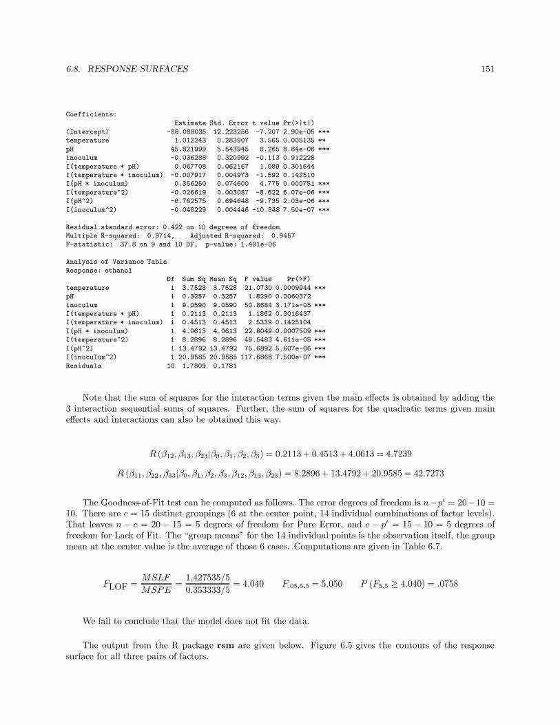
6.8. RESPONSE SURFACES 151
Coefficients:
Estimate Std. Error t value Pr(>|t|)
(Intercept) -88.088035 12.223256 -7.207 2.90e-05 ***
temperature 1.012243 0.283907 3.565 0.005135 **
pH 45.821999 5.543945 8.265 8.84e-06 ***
inoculum -0.036288 0.320992 -0.113 0.912228
I(temperature * pH) 0.067708 0.062167 1.089 0.301644
I(temperature * inoculum) -0.007917 0.004973 -1.592 0.142510
I(pH * inoculum) 0.356250 0.074600 4.775 0.000751 ***
I(temperature^2) -0.026619 0.003087 -8.622 6.07e-06 ***
I(pH^2) -6.762575 0.694648 -9.735 2.03e-06 ***
I(inoculum^2) -0.048229 0.004446 -10.848 7.50e-07 ***
Residual standard error: 0.422 on 10 degrees of freedom
Multiple R-squared: 0.9714, Adjusted R-squared: 0.9457
F-statistic: 37.8 on 9 and 10 DF, p-value: 1.491e-06
Analysis of Variance Table
Response: ethanol
Df Sum Sq Mean Sq F value Pr(>F)
temperature 1 3.7528 3.7528 21.0730 0.0009944 ***
pH 1 0.3257 0.3257 1.8290 0.2060372
inoculum 1 9.0590 9.0590 50.8684 3.171e-05 ***
I(temperature * pH) 1 0.2113 0.2113 1.1862 0.3016437
I(temperature * inoculum) 1 0.4513 0.4513 2.5339 0.1425104
I(pH * inoculum) 1 4.0613 4.0613 22.8049 0.0007509 ***
I(temperature^2) 1 8.2896 8.2896 46.5483 4.611e-05 ***
I(pH^2) 1 13.4792 13.4792 75.6892 5.607e-06 ***
I(inoculum^2) 1 20.9585 20.9585 117.6868 7.500e-07 ***
Residuals 10 1.7809 0.1781
Note that the sum of squares for the interaction terms given the main effects is obtained by adding the3 interaction sequential sums of squares. Further, the sum of squares for the quadratic terms given maineffects and interactions can also be obtained this way.
R (β12, β13, β23|β0, β1, β2, β3) = 0.2113 + 0.4513 + 4.0613 = 4.7239
R (β11, β22, β33|β0, β1, β2, β3, β12, β13, β23) = 8.2896 + 13.4792 + 20.9585 = 42.7273
The Goodness-of-Fit test can be computed as follows. The error degrees of freedom is n−p′ = 20−10 =10. There are c = 15 distinct groupings (6 at the center point, 14 individual combinations of factor levels).That leaves n − c = 20 − 15 = 5 degrees of freedom for Pure Error, and c − p′ = 15 − 10 = 5 degrees offreedom for Lack of Fit. The “group means” for the 14 individual points is the observation itself, the groupmean at the center value is the average of those 6 cases. Computations are given in Table 6.7.
FLOF =MSLF
MSPE=
1.427535/5
0.353333/5= 4.040 F.05,5,5 = 5.050 P (F5,5 ≥ 4.040) = .0758
We fail to conclude that the model does not fit the data.
The output from the R package rsm are given below. Figure 6.5 gives the contours of the responsesurface for all three pairs of factors.

152 CHAPTER 6. MULTIPLE LINEAR REGRESSION
Y X1 X2 X3 Y Grp Y Y − Y Grp Y Grp − Y
4.8 24 3.8 1.59 4.8 5.190776 0 -0.390789.6 24 3.8 10 9.966667 9.971758 -0.36667 -0.0050910.2 24 3.8 10 9.966667 9.971758 0.233333 -0.005098.5 24 3.8 18.41 8.5 7.930448 0 0.5695527.3 24 3.1272 10 7.3 7.170358 0 0.1296424.8 30 4.2 5 4.8 4.920205 0 -0.120217.9 18 3.4 15 7.9 7.90624 0 -0.006246.7 30 3.4 5 6.7 6.329059 0 0.3709419.8 24 3.8 10 9.966667 9.971758 -0.16667 -0.0050910.2 24 3.8 10 9.966667 9.971758 0.233333 -0.005099.8 24 3.8 10 9.966667 9.971758 -0.16667 -0.0050910.2 24 3.8 10 9.966667 9.971758 0.233333 -0.005098.2 18 4.2 15 8.2 8.697386 0 -0.497397.1 18 3.4 5 7.1 7.227422 0 -0.127428.2 13.908 3.8 10 8.2 8.142285 0 0.0577155.6 18 4.2 5 5.6 5.168568 0 0.4314327.5 30 4.2 15 7.5 7.499023 0 0.0009776.7 24 4.4728 10 6.7 6.650866 0 0.0491345.5 30 3.4 15 5.5 6.057877 0 -0.557886.5 34.092 3.8 10 6.5 6.378939 0 0.121061
Sum of Squares 0.353333 1.427535
Table 6.7: Mango Wine Experiment - Lack-of-Fit Test Calculations
R Output - rsm package
Call:
rsm(formula = ethanol ~ SO(temperature, pH, inoculum))
Estimate Std. Error t value Pr(>|t|)
(Intercept) -88.0880353 12.2232556 -7.2066 2.903e-05 ***
temperature 1.0122431 0.2839067 3.5654 0.0051348 **
pH 45.8219993 5.5439454 8.2652 8.839e-06 ***
inoculum -0.0362881 0.3209922 -0.1130 0.9122284
temperature:pH 0.0677083 0.0621670 1.0891 0.3016437
temperature:inoculum -0.0079167 0.0049734 -1.5918 0.1425104
pH:inoculum 0.3562500 0.0746003 4.7754 0.0007509 ***
temperature^2 -0.0266194 0.0030873 -8.6222 6.075e-06 ***
pH^2 -6.7625745 0.6946475 -9.7353 2.032e-06 ***
inoculum^2 -0.0482290 0.0044457 -10.8484 7.500e-07 ***
Multiple R-squared: 0.9714, Adjusted R-squared: 0.9457
F-statistic: 37.8 on 9 and 10 DF, p-value: 1.491e-06
Analysis of Variance Table
Response: ethanol
Df Sum Sq Mean Sq F value Pr(>F)
FO(temperature, pH, inoculum) 3 13.138 4.3792 24.5901 6.227e-05
TWI(temperature, pH, inoculum) 3 4.724 1.5746 8.8417 0.003657
PQ(temperature, pH, inoculum) 3 42.727 14.2424 79.9748 2.730e-07
Residuals 10 1.781 0.1781
Lack of fit 5 1.428 0.2855 4.0402 0.075809
Pure error 5 0.353 0.0707
Stationary point of response surface:
temperature pH inoculum
22.093064 3.811642 11.888138

6.9. TRIGONOMETRIC MODELS 153
temperatureSlice at inoculum = 11.89, temperature = 22.0930636668486, pH = 3.8116424990638
pH
4
5
5
6
6
6
6
7
7
7
8
9
10
15 20 25 30
3.2
3.4
3.6
3.8
4.0
4.2
4.4
temperatureSlice at pH = 3.81, temperature = 22.0930636668486, inoculum = 11.8881378288823
inoculu
m
3
4
4
5
5
5
6
6
7
8
8
9
10
15 20 25 30
510
15
pHSlice at temperature = 22.09, pH = 3.8116424990638, inoculum = 11.8881378288823
inoculu
m
1
2
3
4
5
5
5
6
6
7
7
8
9
10
3.2 3.4 3.6 3.8 4.0 4.2 4.4
510
15
Figure 6.5: Contour Plots of Ethanol for all Pairs of predictors
∇
6.9 Trigonometric Models
Many biological, economic, and meteorological time series of measurements display cyclic patterns, alongwith possibly trend. Use of regression models with sine and cosine components, along with a trend term,can be used to model the process. If there are an even number of k measurements per period, we can includeup to k/2 cosine and (k/2)− 1 sine terms before they start repeating themselves. For monthly (k = 12), wehave the following model, with centered time.
Monthly: Yt = β0 +
5∑
j=1
[
βCj cos
(
2πjt
12
)
+ βSj sin
(
2πjt
12
)]
+ βC6 cos (πt) + β7
(
t− t)
+ εt t = 1, . . . , n
Example: Minneapolis/St.Paul Mean Monthly Temperature - 1/1900-12/2014

154 CHAPTER 6. MULTIPLE LINEAR REGRESSION
This model is fit to monthly mean temperature for Minneapolis/St. Paul, Minnesota over the n = 1380months from 1/1900-12/2014. After fitting the full model, we see that we can drop the two highest ordercosine and the highest order sine term. We then include a plot of the data and the fitted curve for 1/1900-12/1904 in Figure 6.6. A plot pf the full series is so long that you cannot see the pattern. The R programand (partial) output are given below.
### Program
msw <- read.csv("E:\\coursenotes\\minn_stp_weather.csv",header=T)
attach(msw); names(msw)
X1 <- cos(2*pi*1*MonthS/12); X2 <- sin(2*pi*1*MonthS/12)
X3 <- cos(2*pi*2*MonthS/12); X4 <- sin(2*pi*2*MonthS/12)
X5 <- cos(2*pi*3*MonthS/12); X6 <- sin(2*pi*3*MonthS/12)
X7 <- cos(2*pi*4*MonthS/12); X8 <- sin(2*pi*4*MonthS/12)
X9 <- cos(2*pi*5*MonthS/12); X10 <- sin(2*pi*5*MonthS/12)
X11 <- cos(2*pi*6*MonthS/12)
X12 <- MonthS - mean(MonthS)
msw.mod1 <- lm(meanTemp~X1+X2+X3+X4+X5+X6+X7+X8+X9+X10+X11+X12)
summary(msw.mod1)
anova(msw.mod1)
msw.mod2 <- lm(meanTemp~X1+X2+X3+X4+X5+X6+X7+X12)
summary(msw.mod2)
anova(msw.mod2)
plot(msw.mod2)
anova(msw.mod2,msw.mod1)
plot(MonthS[1:60],meanTemp[1:60],pch=16,ylim=c(0,80),
main="Minneapolis-St.Paul Mean Temp1/1900-12/1904")
lines(1:60,predict(msw.mod2)[1:60])
### Output
> summary(msw.mod1)
Coefficients:
Estimate Std. Error t value Pr(>|t|)
(Intercept) 45.269467 0.118994 380.436 < 2e-16 ***
X1 -24.507707 0.168283 -145.634 < 2e-16 ***
X2 -16.183906 0.168283 -96.171 < 2e-16 ***
X3 -1.272425 0.168343 -7.559 7.41e-14 ***
X4 -1.715098 0.168221 -10.195 < 2e-16 ***
X5 0.162471 0.168283 0.965 0.3345
X6 -0.675480 0.168283 -4.014 6.29e-05 ***
X7 -0.278256 0.168343 -1.653 0.0986 .
X8 0.338942 0.168222 2.015 0.0441 *
X9 -0.008014 0.168282 -0.048 0.9620
X10 0.115859 0.168282 0.688 0.4913
X11 0.078679 0.118994 0.661 0.5086
X12 0.001248 0.000297 4.202 2.81e-05 ***
Residual standard error: 4.433 on 1375 degrees of freedom
Multiple R-squared: 0.9571, Adjusted R-squared: 0.9568
F-statistic: 2558 on 12 and 1375 DF, p-value: < 2.2e-16
> summary(msw.mod2)
Coefficients:
Estimate Std. Error t value Pr(>|t|)
(Intercept) 4.527e+01 1.190e-01 380.304 < 2e-16 ***
X1 -2.451e+01 1.683e-01 -145.583 < 2e-16 ***
X2 -1.618e+01 1.683e-01 -96.137 < 2e-16 ***
X3 -1.272e+00 1.684e-01 -7.554 7.63e-14 ***
X4 -1.715e+00 1.683e-01 -10.192 < 2e-16 ***

6.9. TRIGONOMETRIC MODELS 155
0 10 20 30 40 50 60
020
40
60
80
Minneapolis−St.Paul Mean Temp1/1900−12/1904
MonthS[1:60]
meanTem
p[1
:60]
Figure 6.6: Minneapolis/St. Paul Temperatures and Fitted values 1/1900-12/1904
X5 1.630e-01 1.683e-01 0.969 0.333
X6 -6.758e-01 1.683e-01 -4.015 6.28e-05 ***
X7 -2.780e-01 1.684e-01 -1.651 0.099 .
X12 1.248e-03 2.971e-04 4.200 2.84e-05 ***
Residual standard error: 4.435 on 1379 degrees of freedom
Multiple R-squared: 0.957, Adjusted R-squared: 0.9567
F-statistic: 3834 on 8 and 1379 DF, p-value: < 2.2e-16
> anova(msw.mod2,msw.mod1)
Analysis of Variance Table
Model 1: meanTemp ~ X1 + X2 + X3 + X4 + X5 + X6 + X7 + X12
Model 2: meanTemp ~ X1 + X2 + X3 + X4 + X5 + X6 + X7 + X8 + X9 + X10 +
X11 + X12
Res.Df RSS Df Sum of Sq F Pr(>F)
1 1379 27120
2 1375 27023 4 97.52 1.2405 0.2918
The trend coefficient is significant (β = .001248, P < .0001). Above and beyond the cyclic behaviorof the series, temperature has increased by (1380-1)(.001248)=1.72 degrees Fahrenheit on average over theperiod.
∇

156 CHAPTER 6. MULTIPLE LINEAR REGRESSION
6.10 Model Building
When we have many predictors, we may wish to use an algorithm to determine which variables to includein the model. These variables can be main effects, interactions, and polynomial terms. Note that there aretwo common approaches. One method involves testing variables based on t-tests, or equivalently F -testsfor partial regression coefficients. An alternative method involves comparing models based on model basedmeasures, such as Akaike Information Criterion (AIC), or Schwartz Bayesian Information criterion (BICor SBC). These measures can be written as follows (note that different software packages print differentversions, as some parts are constant for all potential models). The goal is to minimize the measures.
AIC(Model) = n ln(SSE(Model))+2p′−n ln(n) BIC(Model) = n ln(SSE(Model))+[ln(n)]p′−n ln(n)
Note that SSE(Model) depends on the variables included in the current model. The measures put apenalty on excess predictor variables, with BIC placing a higher penalty when ln(n) > 2. Note that p′ isthe number of parameters in the model (including the intercept), and n is the sample size. Be aware thatdifferent computer packages can use different formulations of AIC and BIC, unless clearly stated, the goalis still to minimize the values.
Example: Time-to-Incapacitation for Animals Exposed to Burning Aircraft Materials
Spurgeon (1978) reports results from experiments of animals being exposed to n = 71 burning aircraftmaterials. The outcome measured was the time-to-incapacitation. Due to theoretical reasons the responseY is the reciprocal of time-to-incapacitation, multiplied by 1000. For each burned material, levels of p = 7gases were measured: CO, HCN, H2S, HCL, HBr, NO2, and SO2. These were the potential predictors ofY . The R program and output for the full model, containing all predictors main effects (no interactions orquadratic terms are included) are given below.
R Program
toxic <- read.table("http://www.stat.ufl.edu/~winner/data/air_int_incap.dat",
header=F,col.names=c("matcat","matid","timeinc","Y","CO","HCN","H2S",
"HCL","HBr","NO2","SO2"))
attach(toxic)
library(car)
toxic.1 <- lm(Y ~ CO + HCN + H2S + HCL + HBr + NO2 + SO2)
summary(toxic.1)
anova(toxic.1)
drop1(toxic.1,test="F")
vif(toxic.1)
######### Perform Backward Elimination, Forward Selection, and Stepwise Regression
######### Based on Model AIC (not individual regression coefficients)
######### fit1 and fit2 represent "extreme" models
library(MASS)
fit1 <- lm(Y ~ CO + HCN + H2S + HCL + HBr + NO2 + SO2)
fit2 <- lm(Y ~ 1)
stepAIC(fit1,direction="backward")

6.10. MODEL BUILDING 157
stepAIC(fit2,direction="forward",scope=list(upper=fit1,lower=fit2))
stepAIC(fit2,direction="both",scope=list(upper=fit1,lower=fit2))
########## Perform all possible regressions (aka all subset regressions)
########## Prints out best 4 models of each # of predictors
install.packages("leaps")
library(leaps)
alltoxic <- regsubsets(Y ~ CO + HCN + H2S + HCL + HBr + NO2 + SO2,
nbest=4,data=toxic)
aprout <- summary(alltoxic)
n <- length(toxic$Y)
pprime <- apply(aprout$which, 1, sum)
aprout$aic <- aprout$bic - log(n) * pprime + 2 * pprime
with(aprout,round(cbind(which,rsq,adjr2,cp,bic,aic),3)) ## Prints "readable" results
plot(alltoxic,scale="bic")
plot(alltoxic,scale="adjr2")
R Output - Full Model
Coefficients:
Estimate Std. Error t value Pr(>|t|)
(Intercept) 75.44679 15.16710 4.974 5.34e-06 ***
CO 0.64036 0.09717 6.590 1.03e-08 ***
HCN 11.77871 0.90006 13.087 < 2e-16 ***
H2S -10.90998 2.99044 -3.648 0.000537 ***
HCL -0.10200 0.07284 -1.400 0.166337
HBr -0.67569 0.88126 -0.767 0.446105
NO2 44.81628 21.06666 2.127 0.037312 *
SO2 6.61409 2.72454 2.428 0.018069 *
Residual standard error: 55.75 on 63 degrees of freedom
Multiple R-squared: 0.8345, Adjusted R-squared: 0.8161
F-statistic: 45.38 on 7 and 63 DF, p-value: < 2.2e-16
> anova(toxic.1)
Analysis of Variance Table (Sequential SS)
Response: Y
Df Sum Sq Mean Sq F value Pr(>F)
CO 1 81119 81119 26.0966 3.243e-06 ***
HCN 1 787782 787782 253.4359 < 2.2e-16 ***
H2S 1 68561 68561 22.0567 1.478e-05 ***
HCL 1 5208 5208 1.6755 0.200254
HBr 1 2298 2298 0.7392 0.393174
NO2 1 24125 24125 7.7611 0.007044 **
SO2 1 18319 18319 5.8932 0.018069 *
Residuals 63 195830 3108
> drop1(toxic.1,test="F")
Single term deletions
Model:
Y ~ CO + HCN + H2S + HCL + HBr + NO2 + SO2
Df Sum of Sq RSS AIC F value Pr(>F)
<none> 195830 578.48
CO 1 135010 330840 613.72 43.4338 1.028e-08 ***
HCN 1 532345 728174 669.73 171.2595 < 2.2e-16 ***
H2S 1 41373 237203 590.09 13.3100 0.0005374 ***
HCL 1 6095 201925 578.66 1.9608 0.1663369
HBr 1 1827 197657 577.14 0.5879 0.4461054
NO2 1 14068 209897 581.41 4.5256 0.0373116 *
SO2 1 18319 214148 582.83 5.8932 0.0180690 *

158 CHAPTER 6. MULTIPLE LINEAR REGRESSION
Full Model: SSE = 195830 p′ = 7 + 1 = 8 Null Model: TSS = 1183241 p′ = 0 + 1 = 1
Full Model: AIC = 71 ln(195830) + 2(8) − 71 ln(71) = 865.135 + 16 − 302.650 = 578.485
Full Model: BIC = 71 ln(195830) + [ln(71)] (8) − 71 ln(71) = 865.135 + 34.101− 302.650 = 596.586
Null Model: AIC = 71 ln(1183241) + 2(1) − 71 ln(71) = 992.848 + 2 − 302.650 = 692.198
Null Model: BIC = 71 ln(1183241)+ [ln(71)] (1) − 71 ln(71) = 992.848 + 4.263− 302.650 = 694.461
∇
6.10.1 Backward Elimination
This is a “top-down” method, which begins with a “Complete” Model, with all potential predictors. Theanalyst then chooses a significance level to stay in the model (SLS). The model is fit, and the predictorwith the lowest t-statistic in absolute value (largest P -value) is identified. If the P -value is larger than SLS,the variable is dropped from the model. Then the model is re-fit with all other predictors (this will changeall regression coefficients, standard errors, and P -values). The process continues until all variables haveP -values below SLS.
The model based approach fits the full model, with all predictors and computes AIC (or BIC). Then,each variable is dropped one-at-a-time, and AIC (or BIC) is obtained for each model. If none of the modelswith one dropped variable has AIC (or BIC) below that for the full model, the full model is kept, otherwisethe model with the lowest AIC (or BIC) is kept as the new full model. The process continues until novariables should be dropped (none of the ”drop one variable models” has a lower AIC (or BIC) than the“full model.”
Example: Time-to-Incapacitation for Animals Exposed to Burning Aircraft Materials
We make use of the stepAIC command in the R package MASS to use AIC to obtain the BackwardElimination model selection. Note that in the output, RSS is the Residual (Error) Sum of Squares.
R Output - Backward Elimination
> library(MASS)
> fit1 <- lm(Y ~ CO + HCN + H2S + HCL + HBr + NO2 + SO2)
> fit2 <- lm(Y ~ 1)
> stepAIC(fit1,direction="backward")
Start: AIC=578.48
Y ~ CO + HCN + H2S + HCL + HBr + NO2 + SO2
Df Sum of Sq RSS AIC
- HBr 1 1827 197657 577.14
<none> 195830 578.48
- HCL 1 6095 201925 578.66
- NO2 1 14068 209897 581.41

6.10. MODEL BUILDING 159
- SO2 1 18319 214148 582.83
- H2S 1 41373 237203 590.09
- CO 1 135010 330840 613.72
- HCN 1 532345 728174 669.73
Step: AIC=577.14
Y ~ CO + HCN + H2S + HCL + NO2 + SO2
Df Sum of Sq RSS AIC
- HCL 1 5281 202938 577.02
<none> 197657 577.14
- NO2 1 15112 212769 580.38
- SO2 1 17751 215408 581.25
- H2S 1 42033 239690 588.83
- CO 1 154961 352618 616.24
- HCN 1 531912 729569 667.86
Step: AIC=577.02
Y ~ CO + HCN + H2S + NO2 + SO2
Df Sum of Sq RSS AIC
<none> 202938 577.02
- SO2 1 13934 216872 579.73
- NO2 1 21378 224316 582.13
- H2S 1 38630 241568 587.39
- CO 1 166472 369410 617.55
- HCN 1 529032 731971 666.10
Call: lm(formula = Y ~ CO + HCN + H2S + NO2 + SO2)
Coefficients:
(Intercept) CO HCN H2S NO2 SO2
68.4756 0.6211 11.7355 -10.4239 53.2167 5.5480
In the first step, if HBr is removed, SSE = 197657, p′ = 6 + 1 = 7 and AIC drops to 577.14. When themodel drops each of the remaining 6 predictors, one-at-a-time, AIC increases. In the second step, we beginwith the 6 predictor model, and drop each variable, one-at-a-time. The model has AIC = 577.14. WhenHCL is dropped from the model, SSE = 202938, p′ = 5+1 = 6 and AIC drops to 577.02. In the third step,we begin with the 5 predictor model, and drop each variable, one-at-a-time. In each case AIC increases,and we select the 5 predictor model: CO, HCN, H2S, NO2, SO2.
∇
6.10.2 Forward Selection
This is a “bottom-up” method, which begins with all “Simple” Models, each with one predictor. The analystthen chooses a significance level to enter into the model (SLE). Each model is fit, and the predictor withthe highest t-statistic in absolute value (smallest P -value) is identified. If the P -value is smaller than SLE,the variable is entered into the model. Then all two variable models including the best predictor in the firstround, with each of the other predictors. The best second variable is identified, and its P -value is comparedwith SLE. If its P -value is below SLE, the variable is added to the model. The process continues until nopotential added variables have P -values below SLE.
The model based approach fits each simple model, with one predictor and computes AIC (or BIC).The best variable is identified (assuming its AIC (or BIC) is smaller than that for the null model, with nopredictors). Then, each potential variable is added one-at-a-time, and AIC (or BIC) is obtained for each

160 CHAPTER 6. MULTIPLE LINEAR REGRESSION
model. If none of the models with one added variable has AIC (or BIC) below that for the best simplemodel, the simple model is kept, otherwise the model with the lowest AIC (or BIC) is kept as the new fullmodel. The process continues until no variables should be added (none of the ”add one variable models” hasa lower AIC (or BIC) than the “reduced model.”
Example: Time-to-Incapacitation for Animals Exposed to Burning Aircraft Materials
We make use of the stepAIC command in the R package MASS to use AIC to obtain the ForwardSelection model choice. Note that in the output, RSS is the Residual (Error) Sum of Squares for that model.
R Output - Forward Selection
> library(MASS)
> fit1 <- lm(Y ~ CO + HCN + H2S + HCL + HBr + NO2 + SO2)
> fit2 <- lm(Y ~ 1)
> stepAIC(fit2,direction="forward",scope=list(upper=fit1,lower=fit2))
Start: AIC=692.2
Y ~ 1
Df Sum of Sq RSS AIC
+ HCN 1 677833 505408 633.80
+ NO2 1 212831 970410 680.12
+ H2S 1 102071 1081170 687.79
+ CO 1 81119 1102122 689.15
+ HCL 1 51156 1132086 691.06
<none> 1183241 692.20
+ HBr 1 14339 1168902 693.33
+ SO2 1 13344 1169897 693.39
Step: AIC=633.8
Y ~ HCN
Df Sum of Sq RSS AIC
+ CO 1 191068 314340 602.08
+ NO2 1 109591 395817 618.45
+ H2S 1 73868 431541 624.58
+ HCL 1 28118 477291 631.74
+ HBr 1 25890 479518 632.07
<none> 505408 633.80
+ SO2 1 803 504606 635.69
Step: AIC=602.08
Y ~ HCN + CO
Df Sum of Sq RSS AIC
+ H2S 1 68561 245779 586.62
+ NO2 1 65161 249179 587.59
+ SO2 1 14129 300211 600.82
<none> 314340 602.08
+ HCL 1 4387 309953 603.09
+ HBr 1 3701 310639 603.24
Step: AIC=586.62
Y ~ HCN + CO + H2S
Df Sum of Sq RSS AIC
+ NO2 1 28906.7 216872 579.73
+ SO2 1 21462.7 224316 582.13
<none> 245779 586.62
+ HCL 1 5208.0 240571 587.09
+ HBr 1 1509.8 244269 588.18

6.10. MODEL BUILDING 161
Step: AIC=579.73
Y ~ HCN + CO + H2S + NO2
Df Sum of Sq RSS AIC
+ SO2 1 13933.9 202938 577.02
<none> 216872 579.73
+ HCL 1 1463.9 215408 581.25
+ HBr 1 901.2 215971 581.44
Step: AIC=577.02
Y ~ HCN + CO + H2S + NO2 + SO2
Df Sum of Sq RSS AIC
<none> 202938 577.02
+ HCL 1 5280.9 197657 577.14
+ HBr 1 1013.4 201925 578.66
Call: lm(formula = Y ~ HCN + CO + H2S + NO2 + SO2)
Coefficients:
(Intercept) HCN CO H2S NO2 SO2
68.4756 11.7355 0.6211 -10.4239 53.2167 5.5480
In the first stage, each one variable model is compared to the null model. The best single variable isHCN, with AIC = 633.80, compared to the null model with AIC = 692.20. In the second stage, each twovariable model containing HCN is fit, and CO drops AIC to 602.02. The best three variable model containingHCN and CO adds H2S, with AIC = 586.62. In the fourth stage, NO2 is added, with AIC = 579.93, in thefifth stage, SO2 is added with AIC = 577.02. When either HCL or HBr is added, AIC increases.
∇
6.10.3 Stepwise Regression
This approach is a hybrid of forward selection and backward elimination. It begins like forward selection,but then applies backward elimination at each step. In forward selection, once a variable is entered, it staysin the model. In stepwise regression, once a new variable is entered, all previously entered variables aretested, to confirm they should stay in the model, after controlling for the new entrant, as well as the otherprevious entrant.
Example: Time-to-Incapacitation for Animals Exposed to Burning Aircraft Materials
The Stepwise Regression leads to the same model as Backward Elimination and Forward selection forthis data. The output is virtually the same as Forward selection, with the exception that it tries to removepreviously entered predictors at each step.
R Command
stepAIC(fit2,direction="both",scope=list(upper=fit1,lower=fit2))

162 CHAPTER 6. MULTIPLE LINEAR REGRESSION
∇
6.10.4 All Possible Regressions
We can fit all possible regression models, and use model based measures to choose the “best” model. Com-monly used measures are: Adjusted-R2 (equivalently MSE), Mallow’s Cp statistic, AIC, and BIC. Theformulas, and decision criteria are given below (where p′ is the number of parameters in the ”current” modelbeing fit:
Adjusted-R2 - 1 −(
n−1n−p′
)
SSETSS - Goal is to maximize
Mallow’s Cp - Cp =SSE(Model)
MSE(Complete)+ 2p′ − n - Goal is to have Cp ≤ p′
Akaike Information Criterion - AIC(Model) = n ln(SSE(Model)) + 2p′ − n ln(n) - Goal is to minimize
Bayesian Information Criterion - BIC(Model) = n ln(SSE(Model)) + [ln(n)]p′ − n ln(n) - Goal is tominimize
Example: Time-to-Incapacitation for Animals Exposed to Burning Aircraft Materials
The R package leaps will perform all possible regressions. It does not include AIC, however it can becomputed from BIC. The following output gives the best four p = 1, 2, 3, 4, 5, and 6 variable models, aswell as the 7 variable model.
> alltoxic <- regsubsets(Y ~ CO + HCN + H2S + HCL + HBr + NO2 + SO2,
+ nbest=4,data=toxic)
> aprout <- summary(alltoxic)
> n <- length(toxic$Y)
> pprime <- apply(aprout$which, 1, sum)
> aprout$aic <- aprout$bic - log(n) * pprime + 2 * pprime
> with(aprout,round(cbind(which,rsq,adjr2,cp,bic,aic),3)) ## Prints "readable" results
(Intercept) CO HCN H2S HCL HBr NO2 SO2 rsq adjr2 cp bic aic
1 1 0 1 0 0 0 0 0 0.573 0.567 95.594 -51.871 -56.396
1 1 0 0 0 0 0 1 0 0.180 0.168 245.189 -5.554 -10.079
1 1 0 0 1 0 0 0 0 0.086 0.073 280.821 2.120 -2.405
1 1 1 0 0 0 0 0 0 0.069 0.055 287.562 3.483 -1.042
2 1 1 1 0 0 0 0 0 0.734 0.727 36.126 -81.325 -88.113
2 1 0 1 0 0 0 1 0 0.665 0.656 62.338 -64.961 -71.749
2 1 0 1 1 0 0 0 0 0.635 0.625 73.830 -58.826 -65.614
2 1 0 1 0 1 0 0 0 0.597 0.585 88.548 -51.672 -58.460
3 1 1 1 1 0 0 0 0 0.792 0.783 16.069 -94.532 -103.582
3 1 1 1 0 0 0 1 0 0.789 0.780 17.163 -93.556 -102.607
3 1 1 1 0 0 0 0 1 0.746 0.735 33.580 -80.328 -89.378
3 1 1 1 0 1 0 0 0 0.738 0.726 36.714 -78.060 -87.111
4 1 1 1 1 0 0 1 0 0.817 0.806 8.769 -99.153 -110.466
4 1 1 1 1 0 0 0 1 0.810 0.799 11.164 -96.757 -108.070
4 1 1 1 1 1 0 0 0 0.797 0.784 16.394 -91.790 -103.103

6.11. ISSUES OF COLLINEARITY 163
4 1 1 1 0 0 0 1 1 0.796 0.783 16.714 -91.496 -102.809
5 1 1 1 1 0 0 1 1 0.828 0.815 6.287 -99.605 -113.181
5 1 1 1 1 1 0 0 1 0.820 0.806 9.450 -96.246 -109.822
5 1 1 1 1 1 0 1 0 0.818 0.804 10.298 -95.371 -108.947
5 1 1 1 1 0 1 1 0 0.817 0.803 10.480 -95.186 -108.762
6 1 1 1 1 1 0 1 1 0.833 0.817 6.588 -97.214 -113.053
6 1 1 1 1 0 1 1 1 0.829 0.813 7.961 -95.698 -111.536
6 1 1 1 1 1 1 0 1 0.823 0.806 10.526 -92.948 -108.787
6 1 1 1 1 1 1 1 0 0.819 0.802 11.893 -91.525 -107.363
7 1 1 1 1 1 1 1 1 0.834 0.816 8.000 -93.611 -111.712
∇
6.11 Issues of Collinearity
When the predictor variables are highly correlated among themselves, the regression coefficients becomeunstable, with increased standard errors. This leads to smaller t-statistics for tests regarding the partialregression coefficients and wider confidence intervals. At its most extreme case, the sign of a regressioncoefficient can change when a new predictor variable is included. One widely reported measure of collinearityis the Variance Inflation Factor (VIF). This is computed for each predictor variable, by regressing iton the remaining p − 1 predictors. Then V IFJ = 1
1−R2j
where R2j is the coefficent of determination of the
regression of Xj on the remaining predictors. Values of V IFj greater than 10 are considered problematic.Collinearity is not problematic when the primary goal of the model is for prediction.
Various remedies exist. One is determining which variable(s) make the most sense theoretically for themodel, and removing other variables that are correlated with the other more meaningful predictors. A secondmethod involves generating uncorrelated predictor variables from the original set of predictors. While thismethod based on principal components removes the collinearity problem, the new variables may lose theirmeaning, thus making it harder to describe the process. A third method, ridge regression, introduces abias factor into the regression that reduces the inflated variance due to collinearity, and through that reducesthe Mean Square Error of the regression coefficients. Unfortunately, there is no simple rule on choosing thebias factor.
Example: Time-to-Incapacitation for Animals Exposed to Burning Aircraft Materials
The R package car has a vif function that computes the Variance Inflation Factors for each predictor.We apply it to the regression fit on all p = 7 predictors, and find that the gases in their functional forms arenot highly correlated among themselves.
R Output - Variance Inflation Factors
library(car)
toxic.1 <- lm(Y ~ CO + HCN + H2S + HCL + HBr + NO2 + SO2)
vif(toxic.1)

164 CHAPTER 6. MULTIPLE LINEAR REGRESSION
> vif(toxic.1)
CO HCN H2S HCL HBr NO2 SO2
1.483027 2.043812 2.072767 1.223480 1.359955 1.374012 1.189694
∇
6.11.1 Principal Components Regression
For principal components regression, if we have p predictors: X1, . . . , Xp, we can generate p linearly in-dependent predictors that are linear functions of X1, . . . , Xp. When the new variables with small eigenvaluesare removed, the estimate of β obtained from the new regression is biased. The amount of bias depends onthe relative size of the eigenvalues of the removed principal components, however the collinearity problemwill be removed and the variance of the estimator will have been reduced. The process is conducted asfollows (see e.g. Rawlings, Pantula, and Dickey (1998), Section 13.2.2).
1. Create Z1, . . .Zp from the original variables X1, . . . , Xp by subtracting the mean and dividing by amultiple of the standard deviation.
Zij =Xij −Xj√n− 1sj
i = 1, ..., n; j = 1, ..., p Xj =
∑ni=1Xij
nsj =
√
∑ni=1
(
Xij −Xj
)2
n − 1
2. Obtain the eigenvalues λ1, . . . , λp (and place in a diagonal matrix L) and eigenvectors (as columns inmatrix V) of the p× p matrix RXX = Z′Z, where RXX is the correlation matrix among the predictorvariables X1, . . . , Xp. These can be obtained in any matrix computer package (Z does not contain acolumn for an intercept).
R = Z′Z =
1 r12 · · · r1p
r12 1 · · · r2p
......
. . ....
r1p r2p · · · 1
Z′Z = VLV′ =
p∑
i=1
λi (viv′i)
where: Zij =Xij −Xj√n− 1sj
Xj =
∑ni=1Xij
ns2j =
∑ni=1
(
Xij −Xj
)
n− 1
3. The Condition Index for the jth principal component is√
λmaxλj
. Values between 30 and 100 imply
moderate to large depencies among the predictors. Values over 100 are signs of serious collinearityproblems.
4. Create the matrix of principal components W = ZV and augment it with a column of 1s for theintercept: W∗ = [1|W].
5. Fit the regression Y = W∗γ and obtain SSR (γj), the partial sum of squares for each generatedpredictor variable (principal component):
γ = (W∗′
W∗)−1W∗′
Y V γ = s2(W∗′
W∗)−1

6.11. ISSUES OF COLLINEARITY 165
6. For each generated predictor, test H0 : γj = 0, based on the t-test or F -test. Eliminate any principalcomponents with high Condition Index and do not have significant coefficients.
7. Let γ(g) be the vector of retained coefficients from previous part. Then SSRPC =∑
SSR (γj), withg degrees of freedom (the number of retained principal components (generated predictors)).
8. Scaling back to the original variables (in their standardized (mean=0, standard deviation=1) format),
we get: βPC
g = V(g)γ(g)where V(g) is the p × g portion of the eigenvector matrix (columns) corre-sponding to the retained principal components. This ignores the intercept in
9. The estimated variance-covariance matrix of βPC
g is:
V
βPC
g
= s2V(g)L−1(g)V
′(g) L(g) =
λ1 0 · · · 00 λ2 · · · 0...
.... . .
...0 0 · · · λg
10. The fitted regression equation can be written with respect to the original (standardized) variables, orthe principal components:
Y(g) = W∗γ(g)
Note that the bias in the estimation comes when we reduce the principal components regression fromp to g components. If the model reflects no need to remove any principal components, the estimator isunbiased. The bias comes from the fact that we have:
βPC
g = V(g)V′(g)β ⇒ E
βPC
g
= V(g)V′(g)β Note: V(p)V
′(p) = I.
Example: Standing Heights of Female Police Applicants
In a paper describing Principal Components Regression, Lafi and Kaneene (1992) report data fromn = 33 female police applicants, data are in cms, with possibly the exception of Foot Length. The responseif Standing Height (Y ), and the p = 9 predictors are: Sitting Height (X1), Upper Arm Length, (X2),Forearm Length (X3), Hand Length (X4), Upper Leg Length (X5), Lower Leg Length (X6), Foot Length(X7), BRACH (X8 = 100X3/X2), and TIBIO (X9 = 100X6/X5). The data are given in Table 6.8. A typoin the original paper’s table has been corrected, so results differ from authors’.
The correlation matrix among the predictor variables, and its inverse are given below. The diagonalelements of the inverse are the Variance Inflation Factors.

166 CHAPTER 6. MULTIPLE LINEAR REGRESSION
ID Y X1 X2 X3 X4 X5 X6 X7 X8 X9
1 165.8 88.7 31.8 28.1 18.7 40.3 38.9 6.7 88.4 96.52 169.8 90.0 32.4 29.1 18.3 43.3 42.7 6.4 89.8 98.63 170.7 87.7 33.6 29.5 20.7 43.7 41.1 7.2 87.8 94.14 170.9 87.1 31.0 28.2 18.6 43.7 40.6 6.7 91.0 92.95 157.5 81.3 32.1 27.3 17.5 38.1 39.6 6.6 85.0 103.96 165.9 88.2 31.8 29.0 18.6 42.0 40.6 6.5 91.2 96.77 158.7 86.1 30.6 27.8 18.4 40.0 37.0 5.9 90.8 92.58 166.0 88.7 30.2 26.9 17.5 41.6 39.0 5.9 89.1 93.89 158.7 83.7 31.1 27.1 18.1 38.9 37.5 6.1 87.1 96.410 161.5 81.2 32.3 27.8 19.1 42.8 40.1 6.2 86.1 93.711 167.3 88.6 34.8 27.3 18.3 43.1 41.8 7.3 78.4 9712 167.4 83.2 34.3 30.1 19.2 43.4 42.2 6.8 87.8 97.213 159.2 81.5 31.0 27.3 17.5 39.8 39.6 4.9 88.1 99.514 170.0 87.9 34.2 30.9 19.4 43.1 43.7 6.3 90.4 101.415 166.3 88.3 30.6 28.8 18.3 41.8 41.0 5.9 94.1 98.116 169.0 85.6 32.6 28.8 19.1 42.7 42.0 6.0 88.3 98.417 156.2 81.6 31.0 25.6 17.0 44.2 39.0 5.1 82.6 88.218 159.6 86.6 32.7 25.4 17.7 42 37.5 5.0 77.7 89.319 155.0 82.0 30.3 26.6 17.3 37.9 36.1 5.2 87.8 95.320 161.1 84.1 29.5 26.6 17.8 38.6 38.2 5.9 90.2 9921 170.3 88.1 34.0 29.3 18.2 43.2 41.4 5.9 86.2 95.822 167.8 83.9 32.5 28.6 20.2 43.3 42.9 7.2 88.0 99.123 163.1 88.1 31.7 26.9 18.1 40.1 39.0 5.9 84.9 97.324 165.8 87.0 33.2 26.3 19.5 43.2 40.7 5.9 79.2 94.225 175.4 89.6 35.2 30.1 19.1 45.1 44.5 6.3 85.5 98.726 159.8 85.6 31.5 27.1 19.2 42.3 39.0 5.7 86.0 92.227 166.0 84.9 30.5 28.1 17.8 41.2 43.0 6.1 92.1 104.428 161.2 84.1 32.8 29.2 18.4 42.6 41.1 5.9 89.0 96.529 160.4 84.3 30.5 27.8 16.8 41.0 39.8 6.0 91.1 97.130 164.3 85.0 35.0 27.8 19.0 47.2 42.4 5.0 79.4 89.831 165.5 82.6 36.2 28.6 20.2 45.0 42.3 5.6 79.0 94.032 167.2 85.0 33.6 27.1 19.8 46.0 41.6 5.6 80.7 90.433 167.2 83.4 33.5 29.7 19.4 45.2 44.0 5.2 88.7 97.3
Table 6.8: Female Police Applicant Stature Data

6.11. ISSUES OF COLLINEARITY 167
Z =
0.2101 −0.0596 0.0102 0.0242 −0.1584 −0.1437 0.1868 0.0688 0.02150.2973 0.0035 0.1443 −0.0502 0.0774 0.1769 0.1035 0.1258 0.11960.1431 0.1298 0.1980 0.3963 0.1089 0.0419 0.3257 0.0443 −0.09060.1028 −0.1439 0.0236 0.0056 0.1089 −0.0003 0.1868 0.1747 −0.1466
−0.2861 −0.0281 −0.0972 −0.1990 −0.3314 −0.0846 0.1591 −0.0698 0.36700.1766 −0.0596 0.1309 0.0056 −0.0248 −0.0003 0.1313 0.1828 0.03080.0358 −0.1860 −0.0301 −0.0316 −0.1820 −0.3040 −0.0353 0.1665 −0.16530.2101 −0.2281 −0.1508 −0.1990 −0.0562 −0.1353 −0.0353 0.0973 −0.1046
−0.1252 −0.1333 −0.1240 −0.0874 −0.2685 −0.2618 0.0202 0.0158 0.0168−0.2928 −0.0070 −0.0301 0.0987 0.0381 −0.0424 0.0480 −0.0249 −0.1092
0.2034 0.2561 −0.0972 −0.0502 0.0617 0.1010 0.3535 −0.3386 0.0449−0.1587 0.2035 0.2785 0.1173 0.0853 0.1348 0.2146 0.0443 0.0542−0.2727 −0.1439 −0.0972 −0.1990 −0.1977 −0.0846 −0.3131 0.0565 0.1616
0.1565 0.1930 0.3858 0.1545 0.0617 0.2613 0.0757 0.1502 0.25030.1833 −0.1860 0.1041 −0.0502 −0.0405 0.0335 −0.0353 0.3010 0.09620.0022 0.0246 0.1041 0.0987 0.0303 0.1179 −0.0076 0.0647 0.1102
−0.2660 −0.1439 −0.3252 −0.2920 0.1482 −0.1353 −0.2575 −0.1675 −0.36600.0693 0.0351 −0.3521 −0.1618 −0.0248 −0.2618 −0.2853 −0.3671 −0.3147
−0.2392 −0.2175 −0.1911 −0.2362 −0.3471 −0.3800 −0.2297 0.0443 −0.0345−0.0984 −0.3017 −0.1911 −0.1432 −0.2920 −0.2028 −0.0353 0.1421 0.1382
0.1699 0.1719 0.1712 −0.0688 0.0696 0.0672 −0.0353 −0.0209 −0.0112−0.1118 0.0140 0.0772 0.3033 0.0774 0.1938 0.3257 0.0525 0.1429
0.1699 −0.0702 −0.1508 −0.0874 −0.1741 −0.1353 −0.0353 −0.0738 0.05890.0961 0.0877 −0.2313 0.1731 0.0696 0.0082 −0.0353 −0.3060 −0.0859
RXX = Z′Z =
1.0000 0.1441 0.2791 0.1483 0.1863 0.2264 0.3680 0.1146 0.02300.1441 1.0000 0.4708 0.6452 0.7160 0.6616 0.1468 −0.5817 −0.10070.2791 0.4708 1.0000 0.5050 0.3658 0.7284 0.4277 0.4425 0.43960.1483 0.6452 0.5050 1.0000 0.6007 0.5500 0.3471 −0.1901 −0.09940.1863 0.7160 0.3658 0.6007 1.0000 0.7150 −0.0298 −0.3871 −0.41190.2264 0.6616 0.7284 0.5500 0.7150 1.0000 0.2821 0.0028 0.34140.3680 0.1468 0.4277 0.3471 −0.0298 0.2821 1.0000 0.2434 0.39780.1146 −0.5817 0.4425 −0.1901 −0.3871 0.0028 0.2434 1.0000 0.50850.0230 −0.1007 0.4396 −0.0994 −0.4119 0.3414 0.3978 0.5085 1.0000
The V matrix containing the eigenvectors of RXX = Z′Z is obtained using the eigen function in R.
V =
−0.1854 −0.1530 0.8020 −0.2796 0.3690 0.2330 −0.1741 −0.0003 0.0094−0.4414 0.2347 −0.0974 0.2322 0.2543 0.3188 0.3976 0.5776 −0.1693−0.3933 −0.3338 −0.1661 −0.2331 −0.1218 0.3164 0.4962 −0.5132 0.1657−0.4183 0.0807 0.0275 0.2041 −0.5771 0.3718 −0.5521 0.0000 0.0034−0.4127 0.2997 −0.0129 −0.3507 −0.0544 −0.4663 −0.0272 0.1786 0.6031−0.4645 −0.1012 −0.2522 −0.1634 0.2718 −0.3795 −0.2793 −0.1831 −0.5952−0.2140 −0.3578 0.3798 0.5839 −0.2177 −0.4819 0.2477 0.0018 −0.0025
0.0851 −0.5461 −0.0531 −0.4556 −0.3661 −0.0366 0.0417 0.5659 −0.1634−0.0462 −0.5265 −0.3288 0.2714 0.4393 0.1038 −0.3447 0.1315 0.4461

168 CHAPTER 6. MULTIPLE LINEAR REGRESSION
The vector of eigenvalues of RXX = Z′Z is also obtained using the eigen function in R. The eigenvaluesλ and the condition indices are given below.
Eigenvalues:[
3.6299 2.4432 1.0129 0.7666 0.6111 0.3025 0.2326 0.0008 0.0004]
Condition Indices[
1.000 1.219 1.893 2.176 2.437 3.464 3.951 67.174 92.266]
Clearly the eighth and ninth components have very high condition indices.
The matrix of principal components is obtained as W = ZV. When fitting the principal componentregression, we will use W∗ = [1|W].
W =
0.0702 −0.1962 0.2718 0.0926 −0.0397 0.0803 0.0175 0.0004 0.0017−0.2235 −0.2603 0.1604 −0.1467 0.1498 −0.0479 −0.0129 −0.0036 −0.0002−0.4536 −0.0902 0.2193 0.1253 −0.2885 0.0501 0.0052 −0.0012 0.0058−0.0303 −0.1093 0.2012 −0.1149 −0.1798 −0.1746 0.0347 0.0042 0.0007
0.3060 −0.2493 −0.2470 0.4098 0.1611 −0.0297 0.0430 −0.0009 0.0106−0.0639 −0.2547 0.1562 −0.0821 −0.0499 0.0105 0.0376 0.0017 0.0022
0.3462 −0.0567 0.1620 −0.0805 −0.2108 0.1218 0.0673 0.0036 −0.00290.3110 −0.0400 0.2609 −0.1687 0.0452 −0.0653 −0.0216 0.0016 −0.00090.3960 −0.0565 0.0016 0.1612 −0.0739 0.0726 0.0358 −0.0022 −0.00060.0246 0.1308 −0.1608 0.1107 −0.2260 −0.0785 0.0381 −0.0023 −0.0027
−0.2705 0.1005 0.2642 0.3497 0.2718 −0.1407 0.0740 0.0051 −0.0062−0.3614 −0.1290 −0.1639 0.1186 −0.1156 −0.0307 0.1784 −0.0022 −0.0018
0.4207 −0.0303 −0.3452 −0.0567 0.0957 0.0757 −0.0499 −0.0003 −0.0002−0.4923 −0.3438 −0.0813 −0.0780 0.0768 0.1335 0.0197 −0.0053 0.0018
0.0581 −0.3284 0.0775 −0.2519 −0.0123 0.0199 −0.0641 0.0087 −0.0003−0.1587 −0.1149 −0.0878 −0.0329 −0.0058 0.0319 −0.0644 −0.0043 0.0001
0.4223 0.5264 −0.0897 −0.1461 −0.0148 −0.2449 0.0781 −0.0083 0.00160.3540 0.5894 0.1871 0.0046 0.1592 0.0849 0.0128 −0.0052 −0.00290.6885 0.0409 −0.1233 0.0328 −0.0498 0.1382 0.0632 0.0002 −0.00310.5144 −0.2083 −0.0332 0.0604 −0.0299 0.0065 −0.1045 0.0073 0.0011
−0.1995 −0.0043 0.0627 −0.1111 0.1502 0.0817 0.1352 −0.0018 0.0010−0.3365 −0.1978 −0.0714 0.2246 −0.2010 −0.1380 −0.1267 −0.0041 −0.0039
0.2286 −0.0157 0.1732 0.0657 0.1469 0.0953 −0.0737 −0.0036 0.0021−0.0850 0.3421 0.1398 0.1525 0.0665 0.0253 −0.1883 −0.0043 −0.0028−0.6018 −0.0896 0.0491 −0.0812 0.2184 0.0342 0.0313 −0.0033 −0.0019
0.1281 0.1852 0.0946 −0.0350 −0.1600 0.0539 −0.0871 −0.0046 0.00010.0895 −0.4336 −0.2046 −0.0493 0.1614 −0.1362 −0.1607 0.0042 −0.0010
−0.0649 −0.0766 −0.1467 −0.0771 −0.0325 0.0193 0.1064 −0.0027 0.00040.3407 −0.1948 −0.0633 −0.1072 0.0575 −0.1382 0.1137 0.0036 −0.0027
−0.3167 0.6053 −0.0902 −0.1710 0.0774 −0.0187 0.0223 0.0090 0.0087−0.4490 0.4368 −0.2392 0.1438 −0.0288 0.1256 0.0106 0.0144 −0.0052−0.2391 0.4893 0.0133 −0.0281 −0.0911 −0.0498 −0.1099 0.0015 0.0054−0.3521 0.0336 −0.3474 −0.2340 −0.0280 0.0321 −0.0610 −0.0052 −0.0041
The principal component regression coefficients, standard errors, and t-statistics are given in Table 6.10.The estimate of the error variance is s2 = MSE = 3.5737.

6.11. ISSUES OF COLLINEARITY 169
Parameter Estimate Std. Error t-statistic
Intercept 164.5636 0.3275 502.4518W1 -12.1261 0.9875 -12.2792W2 -4.5428 1.2037 -3.7740W3 7.6001 1.8695 4.0654W4 -4.9758 2.1488 -2.3156W5 3.5712 2.4069 1.4837W6 -3.2902 3.4210 -0.9618W7 -6.8250 3.9014 -1.7494W8 22.6248 66.3364 0.3411W9 -37.2527 91.1147 -0.4089
Table 6.9: Female Police Applicant Stature Principal Components Regression - Full Model
Parameter Estimate Std. Error t-statistic
Intercept 164.5636 0.3161 520.6434W1 -12.1261 0.9530 -12.7238W2 -4.5428 1.1616 -3.9107W3 7.6001 1.8041 4.2126W4 -4.9758 2.0737 -2.3994W5 3.5712 2.3228 1.5375W6 -3.2902 3.3015 -0.9966W7 -6.8250 3.7651 -1.8127
Table 6.10: Female Police Applicant Stature Principal Components Regression - Reduced Model
As the standard errors are very large, and the t-statistics are very small for W8 and W9, removethem, and keep the first g = 7 principal components. We create W∗
(7) =[
1|W(7)
]
and compute γ(7) =
(W∗′
(7)W∗(7))
−1W∗(7)Y, and its variance-covariance matrix s2(W∗′
(7)W∗(7))
−1.
The principal component regression coefficients, standard errors, and t-statistics are given in Table ??.The estimate of the error variance is s2 = MSE = 3.2969.
The Principal Component estimates have much smaller standard errors than the OLS estimates. Thepredicted values (not shown here) are very similar for the two methods. The primary difference is thestability of the regression coefficients.
The observed standing heights, and predicted heights from both of the fitted equations (based on W(7)
and Z are given in Table 6.12.
∇
6.11.2 Ridge Regression
In Ridge Regression, a biased estimator is directly induced that reduces its variance and mean squareerror (variance + squared bias). Unfortunately, the bias-inducing constant varies among applications, so it
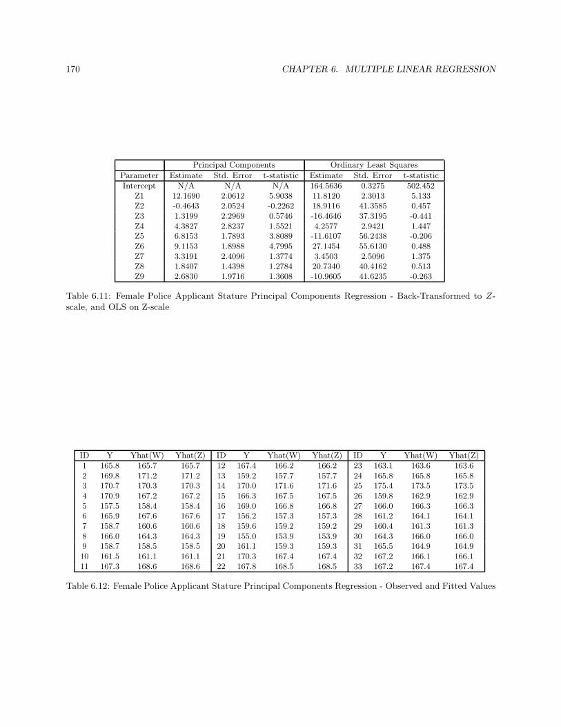
170 CHAPTER 6. MULTIPLE LINEAR REGRESSION
Principal Components Ordinary Least Squares
Parameter Estimate Std. Error t-statistic Estimate Std. Error t-statistic
Intercept N/A N/A N/A 164.5636 0.3275 502.452Z1 12.1690 2.0612 5.9038 11.8120 2.3013 5.133Z2 -0.4643 2.0524 -0.2262 18.9116 41.3585 0.457Z3 1.3199 2.2969 0.5746 -16.4646 37.3195 -0.441Z4 4.3827 2.8237 1.5521 4.2577 2.9421 1.447Z5 6.8153 1.7893 3.8089 -11.6107 56.2438 -0.206Z6 9.1153 1.8988 4.7995 27.1454 55.6130 0.488Z7 3.3191 2.4096 1.3774 3.4503 2.5096 1.375Z8 1.8407 1.4398 1.2784 20.7340 40.4162 0.513Z9 2.6830 1.9716 1.3608 -10.9605 41.6235 -0.263
Table 6.11: Female Police Applicant Stature Principal Components Regression - Back-Transformed to Z-scale, and OLS on Z-scale
ID Y Yhat(W) Yhat(Z) ID Y Yhat(W) Yhat(Z) ID Y Yhat(W) Yhat(Z)
1 165.8 165.7 165.7 12 167.4 166.2 166.2 23 163.1 163.6 163.62 169.8 171.2 171.2 13 159.2 157.7 157.7 24 165.8 165.8 165.83 170.7 170.3 170.3 14 170.0 171.6 171.6 25 175.4 173.5 173.54 170.9 167.2 167.2 15 166.3 167.5 167.5 26 159.8 162.9 162.95 157.5 158.4 158.4 16 169.0 166.8 166.8 27 166.0 166.3 166.36 165.9 167.6 167.6 17 156.2 157.3 157.3 28 161.2 164.1 164.17 158.7 160.6 160.6 18 159.6 159.2 159.2 29 160.4 161.3 161.38 166.0 164.3 164.3 19 155.0 153.9 153.9 30 164.3 166.0 166.09 158.7 158.5 158.5 20 161.1 159.3 159.3 31 165.5 164.9 164.910 161.5 161.1 161.1 21 170.3 167.4 167.4 32 167.2 166.1 166.111 167.3 168.6 168.6 22 167.8 168.5 168.5 33 167.2 167.4 167.4
Table 6.12: Female Police Applicant Stature Principal Components Regression - Observed and Fitted Values

6.11. ISSUES OF COLLINEARITY 171
must be selected comparing results over various possible levels. We begin with a standardized regressionmodel with no bias, based on the p× p correlation matrix among the predictors RXX and the p× 1 vectorof correlations RXY between the predictors and response variable.
RXX =
1 r12 · · · r1p
r12 1 · · · r2p
......
. . ....
r1p r2p · · · 1
RXY =
rY 1
rY 2
...rY p
The estimated standardized regression coefficients are obtained as:
RXXβ∗
= RXY ⇒ β∗
= R−1XXRXY
The standardized regression coefficients β∗
measure the change in Y in standard deviation units as eachpredictor increases by 1 standard deviation, thus removing the effects of scaling each predictor. It can alsobe obtained by transforming each X and Y by the following transformations.
X∗ij =
Xij −Xj√n− 1sj
Y ∗i =
Yi − Y√n− 1sY
In matrix form, we have:
X∗ =
X∗11 X∗
12 · · · X∗1p
X∗21 X∗
22 · · · X∗2p
......
. . ....
X∗n1 X∗
n2 · · · X∗np
Y∗ =
Y ∗1
Y ∗2...Y ∗
n
β∗
=(
X∗′
X∗)−1
X∗′
Y∗
Note that RXX = X∗′
X∗ and RXY = X∗′
Y∗. The standardized ridge estimator is obtained as follows (seee.g. Kutner, Nachtsheim, Neter, and Li (2005), Section 11.2).
β∗
OLS = (RXX)−1
RXY =(
X∗′
X∗)−1
X∗′
Y∗
V
β∗
OLS
= σ2(
X∗′
X∗)−1
β∗
RR = (RXX + cI)−1
RXY =(
X∗′
X∗ + cI)−1
X∗′
Y∗
V
β∗
RR
= σ2(
X∗′
X∗ + cI)−1 (
X∗′
X∗)(
X∗′
X∗ + cI)−1
Making use of the following matrix identity, we can write the Ridge Estimator as a linear function of theOrdinary Least Squares Estimator.
(
A−1 + B−1)−1
= A (A + B)−1 B = B (A + B)−1 A
⇒(
X∗′
X∗ + cI)−1
=1
cI
[
(
X∗′
X∗)−1
+1
cI
]−1(
X∗′
X∗)−1
=
[
c(
X∗′
X∗)−1
+ I
]−1(
X∗′
X∗)−1
⇒ β∗
RR =
[
c(
X∗′
X∗)−1
+ I
]−1
β∗
OLS

172 CHAPTER 6. MULTIPLE LINEAR REGRESSION
A ridge trace plot of the regression coefficients (vertical axis) versus c (horizontal axis) leads to achoice of c, where the coefficients stabilize or “flatten out.” A second graphical measure involves plottingeach of the Variance Inflation Factors versus c, and determining when they all get below 10.
The fitted regression equation in transformed scale is:
Y∗
= X∗βRR ⇒ Y ∗
i = βRR1 X∗
i1 + · · ·+ βRRp X∗
ip.
Yi = β0 + β1Xi1 + · · ·+ βpXip
In terms of the originally scaled response, we have:
βj =
(
sY
sj
)
β∗j β0 = Y − β1X1 − · · · − βpXp.
V IF ≡ Diagonal Elements of R−1 =(
X∗′
X∗)−1
V IF (c) ≡ Diagonal Elements of(
X∗′
X∗ + cI)−1 (
X∗′
X∗)(
X∗′
X∗ + cI)−1
There are also several numerical based approaches (see e.g. Myers (1990), Section 8.4) including GeneralizedCross-Validation (GCV), the “PRESS” Statistic, and the Cc Statistic.
Example: Population and Carbon Emissions in China
Zhu and Peng (2012) fit a model relating China Carbon Emissions (Y in millions of tons) to p = 5predictors: Population
(
X1, in 107)
, Urbanization Rate (X2, in percent), Percent of Population of WorkingAge (X3), Average Household Size (X4), Per Capita Expenditures (X5, adjusted to Year=2000), for n = 31years (1978-2008). The theoretical model was multiplicative, and fit as a linear regression after takinglogarithms. The data in its original units are given in Table 6.13.
lnYt = β0 + β1 lnXt1 + β2 lnXt2 + β3 lnXt3 + β4 lnXt4 + β5 lnXt5 + εt t = 1 . . . , 31
The correlation matrix of the logs of the predictors, RXX , and the vector of correlations of the logs ofthe predictors and the log of the carbon emissions, RXY , are given in Table 6.14. The table also includesR−1
XX , where the Variance Inflation Factors for the predictors are on the main diagonal. Each predictoris highly correlated with emissions, and all of the predictors are highly correlated among themselves. TheVariance Inflation Factors are all well over 10, with the largest, V IF5 = 213.60. This implies the regressionstandard errors will be very large, and the estimates very unstable.
A plot of the Ridge Trace is given in Figure 6.7 and a plot of the VIF is given in Figure 6.8. The V IF s
get below 10 for a very low value of c, around 0.02. The Ridge Trace shows it takes higher values of c, around0.15 or so. The authors used c = 0.20, based on the Ridge Trace. These plots are obtained by “brute force”computing the Ridge Regression coefficients over a grid of c values. The values were c = 0 to 0.5 by 0.0001.All regression coefficients and V IF s were saved and plotted versus c.

6.11. ISSUES OF COLLINEARITY 173
Year Y X1 X2 X3 X4 X5
1978 40.77 96.26 17.92 59.5 4.66 7401979 41.65 97.54 18.96 60 4.65 7911980 40.7 98.71 19.39 60.5 4.61 8621981 40.29 100.07 20.16 61 4.54 9341982 43.12 101.65 21.13 61.5 4.51 9971983 45.47 103.01 21.62 62.37 4.46 10791984 49.43 104.36 23.01 63.24 4.41 12071985 53.59 105.85 23.71 64.12 4.33 13701986 56.35 107.51 24.52 64.99 4.24 14351987 60.12 109.3 25.32 65.86 4.15 15201988 64.45 111.03 25.81 66.15 4.05 16381989 65.47 112.7 26.21 66.45 3.97 16351990 65.86 114.33 26.41 66.74 3.93 16951991 69.15 115.82 26.94 66.3 3.89 18421992 72.14 117.17 27.46 66.2 3.85 20861993 77.02 118.52 27.99 66.7 3.81 22621994 81.81 119.85 28.51 66.6 3.78 23671995 88.47 121.12 29.04 67.2 3.74 25531996 92.6 122.39 30.48 67.2 3.72 27931997 91.49 123.63 31.91 67.5 3.64 29191998 86.61 124.76 33.35 67.6 3.63 30911999 90.5 125.79 34.78 67.7 3.58 33462000 92.89 126.74 36.22 70.15 3.44 36322001 95.14 127.63 37.66 70.4 3.42 38552002 100.96 128.45 39.09 70.3 3.39 41252003 118.72 129.23 40.53 70.4 3.38 44152004 139.07 129.99 41.76 70.92 3.31 47732005 153.42 130.76 42.99 72.04 3.24 51422006 166.46 131.45 43.9 72.32 3.17 56362007 180.17 132.13 44.94 72.53 3.17 62392008 192.27 132.8 45.68 72.8 3.16 6782
Table 6.13: China Carbon Emissions and Population Characteristics 1978-2008
RXX RXY R−1
XX
1.0000 0.9753 0.9712 -0.9873 0.9847 0.9525 50.62 36.87 -9.85 32.98 -44.130.9753 1.0000 0.9801 -0.9907 0.9952 0.9748 36.87 147.72 -27.81 21.50 -134.780.9712 0.9801 1.0000 -0.9802 0.9773 0.9601 -9.85 -27.81 31.40 13.30 19.91-0.9873 -0.9907 -0.9802 1.0000 -0.9942 -0.9786 32.98 21.50 13.30 122.38 54.800.9847 0.9952 0.9773 -0.9942 1.0000 0.9826 -44.13 -134.78 19.91 54.80 213.60
Table 6.14: China Carbon Emissions and Population Characteristics - Correlations and Variance InflationFactors

174 CHAPTER 6. MULTIPLE LINEAR REGRESSION
0.0 0.1 0.2 0.3 0.4 0.5
−4
−3
−2
−1
01
Ridge Trace
c
β^
Figure 6.7: Ridge Trace for China Carbon Data
0.00 0.01 0.02 0.03 0.04 0.05
050
100
150
200
Ridge Trace − VIF
c
VIF
Figure 6.8: VIF versus c for China Carbon Data

6.12. MODELS WITH UNEQUAL VARIANCES (HETEROSKEDASTICITY) 175
Ridge Regression Ordinary Least Squares
Parameter Estimate Std. Error t-statistic Estimate Std. Error t-statistic
(ln X1)∗ 0.1245 0.0163 7.6496 -0.9311 0.1799 -5.1766
(ln X2)∗ 0.2028 0.0126 16.0901 -1.0452 0.3073 -3.4016
(ln X3)∗ 0.1678 0.0175 9.5773 0.2074 0.1417 1.4643
(ln X4)∗ -0.2149 0.0105 -20.5254 -0.7746 0.2797 -2.7698
(ln X5)∗ 0.2337 0.0104 22.4318 1.9668 0.3695 5.3232
Table 6.15: Standardized Regression Coefficients - China Carbon Emissions
Based on using c = 0.20, we get the following estimated standardized regression coefficients, standarderrors, and t-statistics based on Ridge and OLS in Table 6.15.
∇
6.12 Models with Unequal Variances (Heteroskedasticity)
When the data are independent, but with unequal variances, we can use (estimated) Weighted LeastSquares. In rare occasions, the variances are known, and they will be used directly. One setting where thisoccurs in practice is when the “data” are averages among a group of units with common X levels. If eachindividual unit is independent with constant variance σ2, the average of the mi units (Yi in this setting) hasvariance V Yi = σ2/mi. In this case, we would use the reciprocal of the variance as the weight for eachcase (observations based on larger sample sizes have smaller variances and larger weights).
W = Σ−1Y =
1σ21
0 · · · 0
0 1σ22
· · · 0
......
. . ....
0 0 · · · 1σ2
n
=
m1
σ2 0 · · · 00 m2
σ2 · · · 0...
.... . .
...0 0 · · · mn
σ2
βW
= (X′WX)−1
X′WY
The variance of the weighted least squares estimator is obtained as follows:
V
βW
= (X′WX)−1
X′WΣY WX (X′WX)−1
= (X′WX)−1
In the case with V Yi = σ2/mi, we can estimate σ2 based on weighted mean square error:
MSEW =
∑ni=1mi
(
Yi − Yi
)2
n− p′Yi = βW
0 + βW1 Xi1 + · · ·+ βW
p Xip.
In this case (where data are averages):
V
βW
=(
X′WX)−1
W =
m1
MSEW0 · · · 0
0 m2
MSEW· · · 0
......
. . ....
0 0 · · · mn
MSEW

176 CHAPTER 6. MULTIPLE LINEAR REGRESSION
Note that weighted least squares can be conducted as ordinary least squares on transformed X and Y, whichmakes it possible to conduct using EXCEL, and non-statistical computing packages.
X∗ = W1/2X Y∗ = W1/2Y βW
=(
X∗′
X∗)−1
X∗′
Y∗
where W1/2 is the (diagonal) matrix with elements equal to the square roots of the elements of W.
Example: Dose-Response Study of Rosuvastin
Saito, et al (2003) give results of a Japanese Dose-Response study for Rosuvastin in patients with highcholesterol. There were six doses: 1,2.5,5,10,20,40. The response was percentage change in LDL cholesterolat week 12. The data reported were group means per dose, Y j, with varying sample sizes among doses, mj.Assuming equal variances among individual patients, V
Y j
= σ2/mj. The data are given in Table 6.16.Figure 6.9 plots the percentage LDL change (Y ) versus Dose (X) and ln(X). As is often seen with this typeof data, the relationship is curvilinear when Y is plotted versus X, and more linear when it is plotted versusln(X). This analysis will fit the following model.
Y j = β0 + β1 lnXj + εj εj ∼ N
(
0,σ2
mj
)
j = 1, . . . , 6
Y =
−35.8−45.0−52.7−49.7−58.2−66.0
X =
1 0.00001 0.91631 1.60941 2.30261 2.99571 3.6889
W =1
σ2
15 0 0 0 0 00 17 0 0 0 00 0 12 0 0 00 0 0 14 0 00 0 0 0 18 00 0 0 0 0 13
Note that for the Weighted Least Squares estimator, βW
= (X′WX)−1
X′WY, the unknown constant σ2
“cancels out” and does not need to be known. It does need to be estimated to obtain the variance-covariancematrix of β
W.
βW
= (X′WX)−1
X′WY =
[
−36.9588−7.3753
]
YW
= XβW
=
−36.9588−43.7168−48.8289−53.9411−59.0533−64.1654
eW = Y−YW
=
1.1588−1.2832−3.87114.24110.8533−1.8346
SSEW = 15(1.1588)2 + · · ·+ 13(−1.8346)2 = 536.635 s2W = MSEW =536.635
6 − 2= 134.159
V
βW
=(
X′WX)−1
=
[
5.0361 −1.8581−1.8581 0.9786
]
SE
βW0
=√
5.0361 = 2.2441 SE
βW1
=√
0.9786 = 0.9892

6.12. MODELS WITH UNEQUAL VARIANCES (HETEROSKEDASTICITY) 177
Dose Group (j) Change in LDL(
Y j
)
Dose (Xj) ln(Dose) (ln (Xj)) Group Size (mj)
1 -35.8 1 0.0000 152 -45.0 2.5 0.9163 173 -52.7 5 1.6094 124 -49.7 10 2.3026 145 -58.2 20 2.9957 186 -66.0 40 3.6889 13
Table 6.16: Rovustatin Data
The t-tests and Confidence Intervals for β0 and β1 are given below.
β0 : tobs =−36.9588
2.2441= −16.4691 t.025,4 = 2.776 2P (t4 ≥ | − 16.4691|) = .0001
95% CI for β0: − 36.9588± 2.776(2.2441) ≡ −36.9588± 6.2296 ≡ (−43.1884,−30.7292)
β1 : tobs =−7.3753
0.9892= −7.4556 t.025,4 = 2.776 2P (t4 ≥ | − 7.4556|) = .0017
95% CI for β1: − 7.3753± 2.776(0.9892) ≡ −7.3753± 2.7460 ≡ (−10.1213,−4.6293)
A plot of the data and fitted equation is given in Figure 6.10. It also includes the Ordinary Least Squares(OLS) regression line, the two are very similar. The R program using the lm function and weights optionis given below.
The calculations of the Mean, and the Total, Error, and Regression Sums of Squares are obtained below.
Y =
∑nj=1mjY j∑n
j=1mj=
15(−35.8) + · · ·+ 13(−66.0)
15 + · · ·+ 13=
−4535.8
89= −50.9640
TSSW =
n∑
j=1
mj
(
Yj − Y)2
=[
15(−35.8− −50.9640)2 + · · ·+ 13(−66.0−−50.9640)2]
= 7993.945
SSEW =n∑
j=1
mj
(
Yj − Yj
)2
=[
15(−35.8− −36.9588)2 + · · ·+ 13(−66.0−−64.1654)2]
= 536.635
SSRW =
n∑
j=1
mj
(
Yj − Y)2
=[
15(−36.9588−−50.9640)2 + · · ·+ 13(−64.1654−−50.9640)2]
= 7457.310
The F -test for testing H0 : β1 = 0 is as follows.
Fobs =MSRW
MSEW=
7457.310/1
536.635/(6− 2)= 55.584 F.05,1,4 = 7.709 P (F1,4 ≥ 55.584) = .0017
The R program and output are given below.

178 CHAPTER 6. MULTIPLE LINEAR REGRESSION
0 10 20 30 40
−65
−60
−55
−50
−45
−40
−35
dLDL vs Dose
DOSE
dLD
L
0 1 2 3
−65
−60
−55
−50
−45
−40
−35
dLDL vs ln(Dose)
lnDOSE
dLD
L
Figure 6.9: Plots of LDL Change vs Dose and ln(Dose)
0 1 2 3
−65
−60
−55
−50
−45
−40
−35
WLS and OLS Regression of dLDL on ln(DOSE)
ln(DOSE)
dLD
L
WLS
OLS
Figure 6.10: Plot of LDL Change versus ln(Dose) with WLS and OLS Fitted Equations

6.12. MODELS WITH UNEQUAL VARIANCES (HETEROSKEDASTICITY) 179
### Program
dLDL <- c(-35.8,-45.0,-52.7,-49.7,-58.2,-66.0)
DOSE <- c(1,2.5,5,10,20,40)
r <- c(15,17,12,14,18,13)
lnDOSE <- log(DOSE)
cholest <- data.frame(dLDL,lnDOSE,m)
attach(cholest)
cholest.wls <- lm(dLDL ~ lnDOSE, weights=r)
summary(cholest.wls)
confint(cholest.wls)
cholest.ols <- lm(dLDL ~ lnDOSE)
summary(cholest.ols)
confint(cholest.ols)
### Output
Coefficients:
Estimate Std. Error t value Pr(>|t|)
(Intercept) -36.9588 2.2441 -16.469 7.96e-05 ***
lnDOSE -7.3753 0.9892 -7.456 0.00173 **
Residual standard error: 11.58 on 4 degrees of freedom
Multiple R-squared: 0.9329, Adjusted R-squared: 0.9161
F-statistic: 55.59 on 1 and 4 DF, p-value: 0.001729
Analysis of Variance Table
Response: dLDL
Df Sum Sq Mean Sq F value Pr(>F)
lnDOSE 1 7457.3 7457.3 55.586 0.001729 **
Residuals 4 536.6 134.2
> confint(cholest.wls)
2.5 % 97.5 %
(Intercept) -43.18954 -30.728138
lnDOSE -10.12186 -4.628755
###ORDINARY LEAST SQUARES:
Coefficients:
Estimate Std. Error t value Pr(>|t|)
(Intercept) -36.990 2.377 -15.560 9.96e-05 ***
lnDOSE -7.423 1.041 -7.134 0.00204 **
Residual standard error: 3.16 on 4 degrees of freedom
Multiple R-squared: 0.9271, Adjusted R-squared: 0.9089
F-statistic: 50.89 on 1 and 4 DF, p-value: 0.002042
Analysis of Variance Table
Response: dLDL
Df Sum Sq Mean Sq F value Pr(>F)
lnDOSE 1 508.19 508.19 50.89 0.002042 **
Residuals 4 39.94 9.99
> confint(cholest.ols)
2.5 % 97.5 %
(Intercept) -43.58992 -30.38978
lnDOSE -10.31209 -4.53399
∇

180 CHAPTER 6. MULTIPLE LINEAR REGRESSION
6.12.1 Estimated Weighted Least Squares
In most cases, the variances are unknown, and must be estimated. In this case, the squared residuals(variance) or absolute residuals (standard deviation) are regressed against one or more of the predictorvariables or the mean (fitted values). The process is iterative. We begin by fitting ordinary least squares,obtaining the residuals, then regressing the squared or absolute residuals on the the predictor variables orfitted values, leading to (assuming all p predictors are used in the residual regression):
Variance Case: vi = δ0 + δ1Xi1 + · · · δpXip Standard Deviation Case: si = δ0 + δ1Xi1 + · · · δpXip.
Variance Case: vi = δ0 + δ1Yi Standard Deviation Case: si = δ0 + δ1Yi.
Once the estimated variance (standard deviation) is obtained for each case, we get the estimated weights:
Variance Case: wi =1
viStandard Deviation Case: wi =
1
s2i
Then we compute the estimated weighted least squares estimator as:
βW
=(
X′WX)−1
X′WY W =
w1 0 · · · 00 w2 · · · 0...
.... . .
...0 0 · · · wn
.
The process is continued until the estimated regression coefficients are stable from iteration to iteration. Theestimated variance is:
V
βW
= MSEW
(
X′WX)−1
MSEW =1
n− p′
(
Y −XβW)′ (
Y − XβW)
.
It is also possible to estimate the power relation between the standard deviation and the mean σ2 ∝ µδ.The Variance and Standard deviation cases considered above correspond to δ = 1 and 2, respectively.
σ2 = cµδ ⇒ ln(
σ2)
= ln c+ δ lnµ
At each stage in the iteration process, fit a regression of ln(
e2)
on lnY to estimate δ.
Example: Construction Plant Maintenance Costs
Edwards, Holt, and Harris (2000), studied the relationship between Maintenance Costs (Y ) and p = 4predictors: Machine Weight (X1), and indicators for Industry Type (X2 = 1 ifopencast coal, 0 if slate),Machine Type (X3 = 1 if front shovel, 0 if backacter), and Company attitude to Oil Analysis (X4 = 1 ifregular use, 0 if not). The data, fitted values, and residuals are given in Table 6.17, based on a regression ofn = 33 maintenance plants.
The program and output for the regression analysis is given below, as well as the Breusch-Pagan testfor constant error variance. Plots of the residuals and absolute residuals versus fitted values are given in

6.12. MODELS WITH UNEQUAL VARIANCES (HETEROSKEDASTICITY) 181
Plant ID Y X2 X3 X4 X1 YOLS eOLS
1 6.068 1 0 0 16.6 5.028 1.0402 4.602 1 0 0 20.37 5.844 -1.2423 3.282 1 0 0 20.37 5.844 -2.5624 2.192 1 1 0 20.37 1.686 0.5065 2.572 1 1 0 20.37 1.686 0.8866 4.142 1 0 0 20.37 5.844 -1.7027 5.321 1 1 1 21 6.214 -0.8938 4.421 1 1 1 21 6.214 -1.7939 5.301 1 1 1 21 6.214 -0.91310 9.679 1 0 0 27.01 7.283 2.39611 11.997 1 0 1 31 12.538 -0.54112 7.757 1 0 0 31 8.147 -0.39013 12.597 1 0 0 31 8.147 4.45014 13.045 1 0 1 33.2 13.014 0.03115 2.471 0 0 0 45 3.677 -1.20616 6.689 0 0 0 46.27 3.952 2.73717 12.139 1 0 0 46.27 11.454 0.68518 10.859 1 0 0 46.27 11.454 -0.59519 7.119 0 1 0 68.42 4.592 2.52720 3.728 0 1 0 83.7 7.902 -4.17421 46.057 1 1 0 218 44.494 1.56322 49.847 1 1 0 218 44.494 5.35323 61.671 1 1 0 335 69.837 -8.16624 56.167 1 0 1 228 55.209 0.95825 9.721 1 0 1 22.6 10.718 -0.99726 8.535 1 0 1 21.7 10.523 -1.98827 66.91 1 1 1 229 51.268 15.64228 11.101 1 0 1 22.6 10.718 0.38329 12.511 1 0 1 22.6 10.718 1.79330 11.397 1 0 1 31 12.538 -1.14131 4.069 0 0 0 46.27 3.952 0.11732 3.622 1 0 0 20.37 5.844 -2.22233 40.727 1 1 1 229 51.268 -10.541
Table 6.17: Plant Maintenance Cost Data

182 CHAPTER 6. MULTIPLE LINEAR REGRESSION
Figure 6.11. The correlation between the absolute residuals and fitted values is 0.6589, while the correlationbetween the squared residuals and fitted values is 0.5992. We will fit Estimated Weighted Least Squares,based on the Standard deviation case, regressing the absolute residuals on the predicted values.
R Program
cmc <- read.table("http://www.stat.ufl.edu/~winner/data/const_maint.dat",
header=F,col.names=c("mach_id","mach_cost","coal","front_shov","use_oil","mach_wt"))
attach(cmc)
mach.mod1 <- lm(mach_cost ~ mach_wt + coal + front_shov + use_oil)
summary(mach.mod1); anova(mach.mod1)
yhat.1 <- predict(mach.mod1); e.1 <- resid(mach.mod1)
par(mfrow=c(2,1))
plot(yhat.1, e.1)
abline(h=0)
plot(yhat.1, abs(e.1))
abline(lm(abs(e.1) ~ yhat.1))
library(lmtest)
bptest(mach_cost ~ coal + front_shov + use_oil + mach_wt, studentize=F)
plot(yhat.1, abs(e.1))
cor(yhat.1, abs(e.1))
plot(yhat.1, e.1^2)
cor(yhat.1, e.1^2)
print(cbind(cmc,yhat.1,e.1))
R Output - OLS regression and Breusch-Pagan Test
Coefficients:
Estimate Std. Error t value Pr(>|t|)
(Intercept) -6.06990 2.09210 -2.901 0.00716 **
mach_wt 0.21661 0.01041 20.804 < 2e-16 ***
coal 7.50193 2.29401 3.270 0.00285 **
front_shov -4.15823 1.82931 -2.273 0.03089 *
use_oil 4.39110 1.67713 2.618 0.01410 *
Residual standard error: 4.418 on 28 degrees of freedom
Multiple R-squared: 0.9518, Adjusted R-squared: 0.9449
F-statistic: 138.3 on 4 and 28 DF, p-value: < 2.2e-16
Analysis of Variance Table
Response: mach_cost
Df Sum Sq Mean Sq F value Pr(>F)
mach_wt 1 10164.6 10164.6 520.7042 < 2.2e-16 ***
coal 1 413.0 413.0 21.1570 8.281e-05 ***
front_shov 1 88.0 88.0 4.5071 0.04273 *
use_oil 1 133.8 133.8 6.8550 0.01410 *
Residuals 28 546.6 19.5
Breusch-Pagan test
data: mach_cost ~ coal + front_shov + use_oil + mach_wt
BP = 51.742, df = 4, p-value = 1.562e-10
> cor(yhat.1, abs(e.1))
[1] 0.6588788
> cor(yhat.1, e.1^2)
[1] 0.5991547

6.12. MODELS WITH UNEQUAL VARIANCES (HETEROSKEDASTICITY) 183
0 10 20 30 40 50 60 70
−10
05
15
yhat.1
e.1
0 10 20 30 40 50 60 70
05
10
15
yhat.1
abs(e
.1)
Figure 6.11: Residuals vs Fitted (Top) and —Residuals— vs Fitted (Bottom) - Maintenance Costs Example
In the first stage of the EWLS algorithm, we regress the absolute residuals from the OLS regression onthe corresponding fitted values.
R Output - Regression of |e| on Y
> e.reg.ols <- lm(abs.e.ols ~ yhat.ols)
> summary(e.reg.ols)
Coefficients:
Estimate Std. Error t value Pr(>|t|)
(Intercept) 0.64678 0.57616 1.123 0.27
yhat.ols 0.11728 0.02405 4.877 3.06e-05 ***
Residual standard error: 2.499 on 31 degrees of freedom
Multiple R-squared: 0.4341, Adjusted R-squared: 0.4159
F-statistic: 23.78 on 1 and 31 DF, p-value: 3.057e-05
The predicted (fitted) values from this regression are the estimated standard deviations of the obser-vations, as a function of their means. The weights are the inverse of the square of the estimated standarddeviations. The “first round” uses these estimates.
Yi = −6.070+0.217Xi1+7.502Xi2−4.158Xi3+4.391Xi4 si = 0.647+0.117Yi wi =1
s2iW(0) = diagwi

184 CHAPTER 6. MULTIPLE LINEAR REGRESSION
Parameter Estimate Std Error t-statConstant -5.935 1.177 -5.041
X1 0.221 0.017 12.715X2 7.328 1.010 7.256X3 -3.952 0.718 -5.501X4 3.495 0.846 4.130
Table 6.18: Plant Maintenance Cost - Estimated Weighted Least Squares Results
Next, obtain the first iteration of the EWLS estimator and its new prediction and residual vectors.
β(1) =(
X′W(0)X)−1
X′W(0)Y Y(1) = Xβ(1) e(1) = Y − Y(1)
The process continued for 3 iterations until the sum of squared differences of the estimated regressioncoefficient dropped below 0.0001. The iteration history and the final estimated variance-covariance are givenbelow. The final estimates, standard errors, and t-statistics are given in Table 6.18.
βOLS =
−6.06990.21667.5019
−4.15824.3911
β(1) =
−5.93420.22027.3465
−3.98193.5340
β(2) =
−5.93260.22067.3281
−3.95253.4948
βW
=
−5.93460.22067.3275
−3.95213.4954
(
X′W(3)X)−1
=
0.6507 −0.0074 −0.4546 −0.0332 0.0162−0.0074 0.0001 0.0042 −0.0007 −0.0002−0.4546 0.0042 0.4788 −0.0482 −0.1114−0.0332 −0.0007 −0.0482 0.2423 −0.0215
0.0162 −0.0002 −0.1114 −0.0215 0.3363
MSEW =1
n− p′
(
Y − XβW)′(
Y − XβW)
=
(
1
33 − 5
)
(59.6469) = 2.1302
R Program for EWLS
cmc <- read.table("http://www.stat.ufl.edu/~winner/data/const_maint.dat",
header=F,col.names=c("mach_id","mach_cost","coal","front_shov","use_oil","mach_wt"))
attach(cmc)
#### Matrix form (using lm for |e|,y-hat regressions) ###########
n <- length(mach_cost)
X0 <- rep(1,n)

6.12. MODELS WITH UNEQUAL VARIANCES (HETEROSKEDASTICITY) 185
X <- as.matrix(cbind(X0,mach_wt,coal,front_shov,use_oil))
Y <- as.matrix(mach_cost)
p.star <- ncol(X)
#### Fit original regression, and regress |e| on Y-hat
b.ols <- solve(t(X) %*% X) %*% t(X) %*% Y
yhat.ols <- X %*% b.ols
e.ols <- Y - yhat.ols
abs.e.ols <- abs(e.ols)
e.reg.ols <- lm(abs.e.ols ~ yhat.ols)
summary(e.reg.ols)
s.ols <- predict(e.reg.ols)
w.ols <- 1/s.ols^2
b.old <- b.ols
wm.old <- as.matrix(diag(w.ols))
b.diff <- 100
num.iter <- 0
while (b.diff > 0.0001)
num.iter <- num.iter + 1
b.new <- solve(t(X) %*% wm.old %*% X) %*% t(X) %*% wm.old %*% Y
yhat.new <- X %*% b.new
abs.e.new <- abs(Y - yhat.new)
wm.new <- as.matrix(diag(1/predict(lm(abs.e.new~yhat.new))^2))
b.diff <- sum((b.new-b.old)^2)
b.old <- b.new
wm.old <- wm.new
print(b.old)
num.iter
b.wls <- b.new
wm.wls <- wm.new
mse.w <- (t(Y-X%*%b.wls) %*% wm.wls %*% (Y-X%*%b.wls))/(n-p.star)
s2.b.wls <- mse.w[1,1]*solve(t(X) %*% wm.wls %*% X)
s.b.wls <- sqrt(diag(s2.b.wls))
t.b.wls <- b.wls/s.b.wls
print(round(cbind(b.wls,s.b.wls,t.b.wls),3))
∇
Analysis Based on Estimated Variances with Replicated X Values
When the data collection process is based on a well designed controlled experiment, with multiple cases foreach set of X levels, the variance of the errors can be estimated within each distinct group, and used inthe estimated weighted least squares equation directly. If we have g groups of observations with distinctX levels, with the jth having nj observations and sample variance s2j . Then, the vector of responses, Y,its estimated variance-covariance matrix, and the estimated weight matrix for Estimated Weighted LeastSquares (EWLS) are as follow.

186 CHAPTER 6. MULTIPLE LINEAR REGRESSION
Distance (j) Y1j Y2j Y3j Y4j Y5j Y6j Y j sj
10 (1) 3.01 3.02 3.29 3.00 3.20 3.11 3.105 0.11920 (2) 5.57 5.00 5.42 5.73 5.29 5.10 5.353 0.28030 (3) 8.09 6.80 7.95 8.62 8.41 8.62 8.082 0.68540 (4) 10.81 10.19 13.01 11.17 11.33 9.35 10.797 1.23250 (5) 16.07 14.90 17.47 14.21 13.13 11.93 14.618 1.996
Table 6.19: Shotgun Pellet Spread by Distance
Y =
Y1
Y2
...Yg
Yj =
Y1j
Y2j
...Ynjj
ΣY =
s21In1×n1 0n1×n2 · · · 0n1×ng
0n2×n1 s22In2×n2 · · · 0n2×ng
......
. . ....
0ng×n1 0ng×n2 · · · s2gIng×ng
W = Σ−1Y
The EWLS estimator does not need to be iterated, so this is very simple to implement in any matrixspreadsheet or software package.
βW
=(
X′WX)−1
X′WY V
βW
= MSEW
(
X′WX)−1
Example: Shotgun Pellet Spread by Distance
Rowe and Hanson (1985) give results from a forensic experiment to relate shotgun pellet spread asfunction of distance. The data given here are from a Remington 12-gauge shotgun shooting WinchesterSuper X 12-gauge buckshot cartridges. The response Y , was the square root of the area of the smallestrectangle that covered the pellet pattern. There were g = 5 ranges (X,in feet) with nj = 6 replicates perdistance. The data, along with group means and standard deviations are given in Table 6.19. A plot of thedata is given in Figure 6.12. Plots of the mean and standard deviation versus range are given in Figure 6.13.
Clearly the standard deviation (and variance) increase with the mean. Further, the mean of Y is notlinearly related to the range (X), as it bends upward. This leads to fitting a quadratic regression model,with Estimated Weighted Least Squares.
Yij = β0 + β1Xj + β2X2j + εij i = 1, . . . , 6 j = 1, . . .5 Xj = 10j with weights wij =
1
s2j
The R program for the matrix form of Ordinary and Estimated Least Squares are given below and resultsare summarized in Table 6.20.
### Program
sg_spread <- read.csv("http://www.stat.ufl.edu/~winner/sta4210/mydata/shotgun_spread.csv",

6.12. MODELS WITH UNEQUAL VARIANCES (HETEROSKEDASTICITY) 187
10 20 30 40 50
510
15
range
sqrt
A
Figure 6.12: Plot of spread versus Range
10 20 30 40 50
46
812
range1
mean.s
pre
ad
10 20 30 40 50
0.5
1.0
1.5
2.0
range1
sd.s
pre
ad
Figure 6.13: Plots of mean and SD of spread vs Range

188 CHAPTER 6. MULTIPLE LINEAR REGRESSION
header=T)
attach(sg_spread); names(sg_spread)
sg_spread1 <- sg_spread[cartridge==1,]
detach(sg_spread); attach(sg_spread1)
### Matrix Approach
X <- cbind(rep(1,length(sqrtA)),range,range^2)
W <- diag(1/SD_range^2)
Y <- sqrtA
(beta.ols <- solve(t(X) %*% X) %*% t(X) %*% Y)
e.ols <- Y - X %*% beta.ols
(sse.ols <- t(e.ols) %*% e.ols)
(s2.ols <- sse.ols/(length(Y)-ncol(X)))
(v.beta.ols <- s2.ols[1,1] * solve(t(X) %*% X))
se.beta.ols <- sqrt(diag(v.beta.ols))
t.beta.ols <- beta.ols/se.beta.ols
(beta.wls <- solve(t(X) %*% W %*% X) %*% t(X) %*% W %*% Y)
e.wls <- Y - X %*% beta.wls
(sse.wls <- t(e.wls) %*% W %*% e.wls)
(s2.wls <- sse.wls/(length(Y)-ncol(X)))
(v.beta.wls <- s2.wls[1,1] * solve(t(X) %*% W %*% X))
se.beta.wls <- sqrt(diag(v.beta.wls))
t.beta.wls <- beta.wls/se.beta.wls
print(round(cbind(beta.ols,se.beta.ols,t.beta.ols,
beta.wls,se.beta.wls,t.beta.wls),4))
### Output
> (beta.ols <- solve(t(X) %*% X) %*% t(X) %*% Y)
1.308666667
range 0.159873810
0.002110714
> (sse.ols <- t(e.ols) %*% e.ols)
[1,] 30.43237
> (s2.ols <- sse.ols/(length(Y)-ncol(X)))
[1,] 1.127125
> (v.beta.ols <- s2.ols[1,1] * solve(t(X) %*% X))
0.8641289841 -6.199186e-02 9.392706e-04
range -0.0619918619 5.018389e-03 -8.050891e-05
0.0009392706 -8.050891e-05 1.341815e-06
> (beta.wls <- solve(t(X) %*% W %*% X) %*% t(X) %*% W %*% Y)
1.255644821
range 0.164596451
0.002029814
> (sse.wls <- t(e.wls) %*% W %*% e.wls)
[1,] 25.09147
> (s2.wls <- sse.wls/(length(Y)-ncol(X)))
[1,] 0.9293137
> (v.beta.wls <- s2.wls[1,1] * solve(t(X) %*% W %*% X))
0.059140712 -6.868167e-03 1.494750e-04
range -0.006868167 8.380629e-04 -1.895007e-05
0.000149475 -1.895007e-05 4.603523e-07
The R commands and output for OLS and EWLS (with the weight statement are given below, usingthe lm function.

6.12. MODELS WITH UNEQUAL VARIANCES (HETEROSKEDASTICITY) 189
Ordinary Least Squares Estimated Weighted Least Squares OLS - Robust SEs
Parameter Estimate Std Error t-stat Estimate Std Error t-stat Estimate Std Error t-statConstant 1.30867 0.92959 1.408 1.25564 0.24319 5.163 1.30867 0.56985 2.297
X 0.15987 0.07084 2.257 0.16460 0.02895 5.686 0.15987 0.05921 2.700X2 0.00211 0.00116 1.822 0.00203 0.00068 2.992 0.00211 0.00118 1.795
Table 6.20: OLS and EWLS estimates, standard errors, and t-tests
### Program
sg_spread <- read.csv("http://www.stat.ufl.edu/~winner/sta4210/mydata/shotgun_spread.csv",
header=T)
attach(sg_spread); names(sg_spread)
sg_spread1 <- sg_spread[cartridge==1,]
detach(sg_spread); attach(sg_spread1)
regweight <- 1/(SD_range^2)
### Ordinary Least Squares
sg.mod1 <- lm(sqrtA ~ range + I(range^2))
summary(sg.mod1)
#### Weighted Least Squares
sg.mod2 <- lm(sqrtA ~ range + I(range^2),
weight=regweight)
summary(sg.mod2)
### Output
> ### Ordinary Least Squares
> sg.mod1 <- lm(sqrtA ~ range + I(range^2))
> summary(sg.mod1)
Coefficients:
Estimate Std. Error t value Pr(>|t|)
(Intercept) 1.308667 0.929585 1.408 0.1706
range 0.159874 0.070841 2.257 0.0323 *
I(range^2) 0.002111 0.001158 1.822 0.0795 .
Residual standard error: 1.062 on 27 degrees of freedom
Multiple R-squared: 0.9422, Adjusted R-squared: 0.9379
F-statistic: 220.2 on 2 and 27 DF, p-value: < 2.2e-16
> #### Weighted Least Squares
> sg.mod2 <- lm(sqrtA ~ range + I(range^2),
+ weight=regweight)
> summary(sg.mod2)
Coefficients:
Estimate Std. Error t value Pr(>|t|)
(Intercept) 1.2556448 0.2431886 5.163 1.96e-05 ***
range 0.1645965 0.0289493 5.686 4.86e-06 ***
I(range^2) 0.0020298 0.0006785 2.992 0.00586 **
Residual standard error: 0.964 on 27 degrees of freedom
Multiple R-squared: 0.9754, Adjusted R-squared: 0.9736
F-statistic: 535.4 on 2 and 27 DF, p-value: < 2.2e-16
∇

190 CHAPTER 6. MULTIPLE LINEAR REGRESSION
Robust Standard Errors
In general, the variance-covariance matrix of the Ordinary Least Squares estimator is:
V
β
= V
(X′X)−1
X′Y
= (X′X)−1
X′ΣYX (X′X)−1
A simple, yet effective method is to obtain robust standard errors of the ordinary least squares (OLS)estimators based on the residuals from the linear regression (using the squared residuals as estimates of thevariances for the individual cases). This method was originally proposed by White (1980). The estimatedvariance-covariance matrix with resulting robust to heteroskedasticity standard errors for β is:
V
β
= (X′X)−1X′E2X(X′X)−1 E2 =
e21 0 · · · 00 e22 · · · 0...
.... . .
...0 0 · · · e2n
= diag (ee′) .
Example: Shotgun Pellet Spread by Distance
For the shotgun pellet spread data, we obtain the OLS estimator for β and obtain robust standard errorsin matrix form. The results for the estimated coefficients, robust standard errors and t-statistics are givenin Table 6.20.
### Robust Standard Errors
(beta.ols <- solve(t(X) %*% X) %*% t(X) %*% Y)
e.ols <- Y - X %*% beta.ols
E2 <- e.ols %*% t(e.ols) * diag(length(Y))
(v.beta.ols.robust<- solve(t(X) %*% X) %*% t(X) %*% E2 %*%
X %*% solve(t(X) %*% X))
se.beta.ols.robust <- sqrt(diag(v.beta.ols.robust))
t.beta.ols.robust <- beta.ols/se.beta.ols.robust
print(round(cbind(beta.ols,se.beta.ols.robust,t.beta.ols.robust),5))
> (v.beta.ols.robust<- solve(t(X) %*% X) %*% t(X) %*% E2 %*%
+ X %*% solve(t(X) %*% X))
range
0.3247278501 -3.349684e-02 6.465852e-04
range -0.0334968425 3.505749e-03 -6.867561e-05
0.0006465852 -6.867561e-05 1.383327e-06
∇

6.12. MODELS WITH UNEQUAL VARIANCES (HETEROSKEDASTICITY) 191
6.12.2 Bootstrap Methods When Distribution of Errors is Unknown
The bootstrap is widely used in many applications when the distribution of the data is unknown, or whenthe distribution of the estimator of is unknown. In regression applications, there are various ways of boot-strapping (see e.g. Cameron and Trivedi (2009, Chapter 13) and Kutner, et al (2005, Section 11.5)). Allsampling is done with replacement (except the parametric bootstrap).
One possibility is to bootstrap the individual cases from the dataset, and repeatedly re-fit the regression,and saving the regression coefficients, obtaining their standard error. Then we can construct ConfidenceIntervals for the regression coefficients by taking the original estimate and adding and subtracting 2 standarderrors for approximate 95% Confidence Intervals. This method is widely used when the X levels are random(not set up by the experimenter), and when the errors may not have constant variance. Also, the cut-offvalues for the middle (1 − α)100% of the bootstrap estimates can be used.
Another possibility that is useful is to retain the fitted values from the original regression Y1, . . . , Yn andbootstrap the residuals e1, . . . , en. Then the bootstrapped residuals are added to the original fitted valuesand the regression coefficients are obtained, and their standard error is computed and used as above.
The reflection method (see e.g. Kutner, et al (2005, Section 11.5)) is another possibility. In this case, we
obtain the lower α/2 percentile of the bootstrapped regression coefficients(
β∗j (α/2)
)
and the upper 1−α/2
percentile of the regression coefficients(
β∗j (1 − α/2)
)
and obtain the interval:
βj − β∗j (α/2) ≤ βj ≤ β∗
j (1 − α/2) − βj j = 0, 1, . . . , p.
In the parametric bootstrap, the residuals are sampled from a specified distribution with parameter(s)estimated from the original sample.
There are various bias-corrected methods applied as well that are computed by statistical softwarepackages.
Example: Total Phenolic Content and DPPH Radical Scavenging Activity in Lager Beers
Zhao, Li, Sun, Yang, and Zhao (2013) report the results of a study relating antioxidant activity tophenolic content in n = 40 lager beers. The response is DPPH Radical Scavenging Activity (Y ), and thepredictor is Total Phenolic Content (X). The data are given in Table 6.21 and plotted in Figure 6.14 alongwith the OLS simple linear regression line.
The standard output for the regression model is given below.
lager <- read.csv("http://www.stat.ufl.edu/~winner/data/lager_antioxidant_reg.csv",
header=T)
attach(lager); names(lager)
# print(cbind(tpc,dsa))

192 CHAPTER 6. MULTIPLE LINEAR REGRESSION
Lager ID X Y Lager ID X Y Lager ID X Y Lager ID X Y
1 148.23 0.66 11 169.51 0.53 21 159.81 0.56 31 177.83 0.632 160.38 0.63 12 111.05 0.32 22 163.23 0.56 32 150.11 0.643 170.41 0.62 13 143.50 0.42 23 169.59 0.53 33 135.92 0.484 208.65 0.90 14 186.96 0.64 24 135.76 0.49 34 162.99 0.965 146.03 0.64 15 109.50 0.42 25 198.62 0.58 35 183.54 0.636 180.19 0.62 16 209.95 0.77 26 221.94 0.68 36 236.37 0.867 169.06 0.58 17 88.47 0.30 27 148.80 0.56 37 163.23 0.588 119.04 0.47 18 230.25 0.70 28 120.02 0.36 38 212.48 0.809 158.99 0.59 19 152.96 0.51 29 84.64 0.24 39 235.06 0.7510 153.04 0.72 20 147.42 0.53 30 238.33 0.97 40 267.27 0.91
Table 6.21: Total Phenolic Content (X) and DPPH Radical Scavenging Activity (Y ) for 40 lager beers
100 150 200 250
0.4
0.6
0.8
DPPH versus TPC
tpc
dsa
Figure 6.14: Plot of DPPH Radical Scavenging Activity vs Total Phenolic Content and Fitted Equation -Lager Beer Data

6.12. MODELS WITH UNEQUAL VARIANCES (HETEROSKEDASTICITY) 193
lager.mod1 <- lm(dsa ~ tpc)
summary(lager.mod1)
anova(lager.mod1)
confint(lager.mod1)
plot(tpc,dsa, main="DPPH versus TPC")
abline(lager.mod1)
Coefficients:
Estimate Std. Error t value Pr(>|t|)
(Intercept) 0.0343018 0.0639781 0.536 0.595
tpc 0.0034132 0.0003694 9.240 2.93e-11 ***
Residual standard error: 0.09629 on 38 degrees of freedom
Multiple R-squared: 0.692, Adjusted R-squared: 0.6839
F-statistic: 85.38 on 1 and 38 DF, p-value: 2.926e-11
> anova(lager.mod1)
Analysis of Variance Table
Response: dsa
Df Sum Sq Mean Sq F value Pr(>F)
tpc 1 0.79175 0.79175 85.385 2.926e-11 ***
Residuals 38 0.35236 0.00927
> confint(lager.mod1)
2.5 % 97.5 %
(Intercept) -0.09521518 0.163818791
tpc 0.00266544 0.004160979
We next apply the two versions of the bootstrap. The first involves saving the fitted values and residualsfrom the regression of the actual dataset, then bootstrapping the residuals and adding them to the fixedfitted values for the “new data” and regressing them on the original X values. The program below fits theoriginal regression, and saves Y and e, and the estimated slope β1 .
lager <-
read.csv("http://www.stat.ufl.edu/~winner/sta4210/mydata/lager_antioxidant_reg.csv",
header=TRUE)
attach(lager); names(lager)
lager.mod1 <- lm(dsa ~ tpc)
summary(lager.mod1)
confint(lager.mod1)
yhat <- predict(lager.mod1)
e <- residuals(lager.mod1)
b1 <- coef(lager.mod1)[2]
The following part of the program sets up the “fixed” X matrix and Y vector. Then it samples n = 40elements of e with replacement, and adds them to Y to obtain Yboot. We then obtain the least squares
estimate βboot = (X′X)−1
X′Yboot. We then save the estimated slope β1,boot. The process is repeated10000 times. Confidence intervals for β1 are obtained directly from the empirical “bootstrap distribution”and from the reflection method. The histogram is given in Figure 6.15.
############## Bootstrap w/ Fixed X’s. Adds random errors to predicted values
n <- length(dsa)
X <- as.matrix(cbind(rep(1,n),tpc))

194 CHAPTER 6. MULTIPLE LINEAR REGRESSION
set.seed(13579)
num.boot <- 10000
b1.boot <- rep(0,num.boot)
for (i in 1:num.boot)
e.boot <- as.matrix(sample(e,size=n,replace=TRUE))
Y.boot <- yhat + e.boot
b.boot <- solve(t(X) %*% X) %*% t(X) %*% Y.boot
b1.boot[i] <- b.boot[2,1]
hist(b1.boot, breaks=24,main="Bootstrap Method 1")
(b1.boot_025 <- quantile(b1.boot,.025))
(b1.boot_975 <- quantile(b1.boot,.975))
(b1.boot.sd <- sd(b1.boot))
(d1 <- b1-b1.boot_025)
(d2 <- b1.boot_975-b1)
(beta1.95CI <- c(b1-d2,b1+d1))
> (b1.boot_025 <- quantile(b1.boot,.025))
2.5%
0.002700025
> (b1.boot_975 <- quantile(b1.boot,.975))
97.5%
0.004141108
> (b1.boot.sd <- sd(b1.boot))
[1] 0.0003603104
> (d1 <- b1-b1.boot_025)
0.0007131838
> (d2 <- b1.boot_975-b1)
0.0007278994
> (beta1.95CI <- c(b1-d2,b1+d1))
tpc tpc
0.002685310 0.004126393
The second method involves sampling the observed (X, Y ) pairs with replacement for samples of sizen = 40, and fitting the regression on each sample, saving the estimated slope each time. The program andoutput are given below, and the histogram is given in Figure 6.16.
###### Bootstrap by selecting n (X,Y) pairs with replacement
num.boot <- 10000
set.seed(34567)
b1.boot <- rep(0,num.boot)
for (i in 1:num.boot)
boot.sample <- sample(1:n,size=n,replace=TRUE)
dsa.b <- dsa[boot.sample]
tpc.b <- tpc[boot.sample]
X.boot <- as.matrix(cbind(rep(1,n),tpc.b))
Y.boot <- dsa.b
b.boot <- solve(t(X.boot) %*% X.boot) %*% t(X.boot) %*% Y.boot
b1.boot[i] <- b.boot[2,1]
hist(b1.boot, breaks=24,main="Bootstrap Method 2")

6.12. MODELS WITH UNEQUAL VARIANCES (HETEROSKEDASTICITY) 195
Bootstrap Method 1
b1.boot
Fre
quency
0.0020 0.0025 0.0030 0.0035 0.0040 0.0045 0.0050
0200
400
600
800
1000
Figure 6.15: Histogram of Bootstrap Estimates of Regression Slope - Method 1
Bootstrap Method 2
b1.boot
Fre
quency
0.0015 0.0020 0.0025 0.0030 0.0035 0.0040 0.0045
0200
400
600
800
1000
1200
Figure 6.16: Histogram of Bootstrap Estimates of Regression Slope - Method 2

196 CHAPTER 6. MULTIPLE LINEAR REGRESSION
(b1.boot_025 <- quantile(b1.boot,.025))
(b1.boot_975 <- quantile(b1.boot,.975))
(b1.boot.sd <- sd(b1.boot))
(d1 <- b1-b1.boot_025)
(d2 <- b1.boot_975-b1)
(beta1.95CI <- c(b1-d2,b1+d1))
> (b1.boot_025 <- quantile(b1.boot,.025))
0.002754063
> (b1.boot_975 <- quantile(b1.boot,.975))
0.004018062
> (b1.boot.sd <- sd(b1.boot))
[1] 0.0003181617
> (d1 <- b1-b1.boot_025)
0.0006591461
> (d2 <- b1.boot_975-b1)
0.0006048525
> (beta1.95CI <- c(b1-d2,b1+d1))
0.002808357 0.004072355
The original interval, based on the t-distribution and the bootstrap intervals are very similar in thiscase, as the data are very “well-behaved” in terms of their residuals.
∇
6.13 Generalized Least Squares for Correlated Errors
Typically when data are collected over time and/or space, the errors are correlated, with correlation tendingto be higher among observations that are closer in time or space. In this case, the variance-covariance matrixof the error terms is written generally:
V ε = Σ =
σ21 σ12 · · · σ1n
σ12 σ22 · · · σ2n
......
. . ....
σ1n σ2n · · · σ2n
.
For the case where the observations are equally spaced in time, and the error terms form an autoregressiveprocess of order 1, we have:
εt = νt + ρεt−1 − 1 < ρ < 1 νt ∼ iid(
0, σ2)
νt+k ⊥ εt ∀ k > 0
Note that this autoregressive process can extend back to q time points, but the covariance structure gets
more complicated. If we start with the definition that E ε1 = 0 and V ε1 = σ2
1−ρ2 , we obtain:
E ε2 = E ν2 + ρε1 = 0
V ε2 = V ν2 + ρε1 = V ν2 + V ρε1 + 2COV ν2, ρε1 = σ2 +ρ2σ2
1 − ρ2+ 2(0) =
σ2
1 − ρ2.

6.13. GENERALIZED LEAST SQUARES FOR CORRELATED ERRORS 197
COV ε1, ε2 = COV ε1, ν2 + ρε1 =ρσ2
1 − ρ2
In general, this extends to the following results.
V εt =σ2
1 − ρ2= γ(0) COV εt, εt+k =
ρ|k|σ2
1 − ρ2= γ(k) ρ =
COV εt, εt+1V εt
=γ(1)
γ(0)
V ε = Σ =σ2
1 − ρ2
1 ρ · · · ρn−1
ρ 1 · · · ρn−2
......
. . ....
ρn−1 ρn−2 · · · 1
If ρ were known, then we could use Generalized Least Squares to estimate β. Let Σ = σ2W. Then wewould have:
βGLS
=(
X′W−1X)−1
X′W−1Y s2 =1
n− p′
(
Y − XβGLS
)′ (
Y − XβGLS
)
V
βGLS
= s2(
X′W−1X)−1
.
In practice, ρ will be unknown, and can be estimated from the data. Further, if we make the followingtransformations for AR(1) errors, the transformed response will have uncorrelated errors:
Y∗ = T−1Y X∗ = T−1X T−1 =
√
1 − ρ2 0 0 · · · 0 0 0−ρ 1 0 · · · 0 0 00 −ρ 1 · · · 0 0 0...
.... . .
. . ....
......
......
.... . .
. . ....
...0 0 0 · · · −ρ 1 00 0 0 · · · 0 −ρ 1
For this model, the transformed Y∗, has the following model and variance-covariance structure:
Y∗ = X∗β + T−1ε V Y∗ = T−1σ2WT−1′
= σ2I
Then for Estimated Generalized Least Squares (EGLS), also known as Feasible Generalized LeastSquares (FGLS), we obtain estimates of ρ and σ2 based on the residuals from the OLS regression, thenre-fit the EGLS model.
γ(0) =
∑nt=1 e
2t
nγ(1) =
∑nt=2 etet−1
nρ =
γ(1)
γ(0)σ2 = γ(0) − ργ(1)
Next, we obtain the “estimated” transformation matrix, and the transformed Y∗ and X∗:
Y∗ = T−1Y X∗ = T−1X T−1 =
√
1 − ρ2 0 0 · · · 0 0 0−ρ 1 0 · · · 0 0 00 −ρ 1 · · · 0 0 0...
.... . .
. . ....
......
......
.... . .
. . ....
...0 0 0 · · · −ρ 1 00 0 0 · · · 0 −ρ 1

198 CHAPTER 6. MULTIPLE LINEAR REGRESSION
Note that the transformed responses have the following pattern (the predictors (and intercept) will have asimilar structure).
Y ∗1 =
√
1 − ρ2Y1 Y ∗t = Yt − ρYt−1 t = 2, . . . , n
The EGLS estimator, its variance-covariance matrix, and the estimator for σ2 are obtained as follow.
βEGLS
=(
X′T−1′
T−1X)−1
X′T−1′
T−1Y =(
X∗′
X∗)−1
X∗′
Y∗
V
βEGLS
= σ2e
(
X′T−1′
T−1X)−1
= σ2e
(
X∗′
X∗)−1
σ2e =
(
Y − XβEGLS
)′
T−1′
T−1(
Y −XβEGLS
)
n− p′ − 1=
(
Y∗ − X∗βEGLS
)′ (
Y∗ − X∗βEGLS
)
n− p′ − 1
Tests and Confidence Intervals for regression coefficients are obtained as follow.
H0 : βj = 0 HA : βj 6= 0 TS : tobs =βEGLS
j
SE
βEGLSj
RR : |tobs| ≥ t (n− p′ − 1, α/2)
(1 − α)100% Confidence Interval: βEGLSj ± t (n− p′ − 1, α/2) SE
βEGLSj
A test for the autoregressive parameter ρ is obtained as follows:
s2 =γ(0) − ργ(1)
n− p′ − 1SE ρ =
√
s2
γ(0)tobs =
ρ
SE ρ
This procedure was first described by Gallant and Goebel (1976) that can be applied to linear or nonlinearregression problems. The method is the basis for the Autoreg procedure in SAS. R has a function gls inthe nlme (nonlinear mixed effects) package. If you use method=”ML” as an option, it uses MaximumLikelihood, and will obtain slightly different estimates than this method. The ML method is an iterativeprocedure. Note that the gls function has Restricted Maximum Likelihood (REML) as the default. Thisgives totally different and inappropriate estimates for regression models.
Example: U.S. Annual Wine Consumption and Adult Population 1934-2002
Table 6.22 contains annual U.S. adult population (X, in millions) and wine consumption (Y , in millionsof gallons) for the years 1934-2003. Note that 1934 was the first year after Prohibition was repealed. A plotof the data and ordinary least squares regression line is given in Figure 6.17, and a plot of residuals versustime is given in Figure 6.18. As population is increasing over time, the plot of wine sales versus populationhas an inherent “time effect” contained in it, and shows periodic behavior in the top portion. The residualsdisplay clear autocorrelation.
We first give the analysis based on the lm (OLS) and gls (EGLS) functions, as well as the Durbin-Watsontest. The Durbin-Watson statistic is very small, demonstrating very strong evidence of autocorrelation of theerror terms. The lmtest package has the dwtest function, that provides a P -value, based on an assumptionof normality, computed by the “pan” algorithm.

6.13. GENERALIZED LEAST SQUARES FOR CORRELATED ERRORS 199
Year Wine (Y) Pop(X) Year Wine (Y) Pop(X) Year Wine (Y) Pop(X)
1934 33 91.642 1957 152 119.383 1980 480 175.9351935 46 92.868 1958 155 121.052 1981 506 178.2121936 60 94.068 1959 156 123.091 1982 514 180.3341937 67 95.251 1960 163 124.594 1983 528 182.3241938 67 96.504 1961 172 126.137 1984 555 184.3431939 77 97.760 1962 168 128.634 1985 580 186.3891940 90 99.181 1963 176 130.777 1986 587 188.5991941 101 100.463 1964 186 132.942 1987 581 190.4301942 113 101.734 1965 190 135.052 1988 551 192.0471943 98 103.023 1966 191 137.301 1989 524 193.5981944 99 104.300 1967 203 139.653 1990 509 195.4771945 94 105.350 1968 214 142.022 1991 466 197.7351946 140 106.301 1969 236 144.417 1992 476 200.3091947 97 107.462 1970 267 147.114 1993 449 202.8241948 122 108.623 1971 305 149.927 1994 459 205.3241949 133 109.812 1972 337 152.849 1995 464 208.0061950 140 110.875 1973 347 155.749 1996 500 210.6911951 127 111.981 1974 349 158.651 1997 520 213.5601952 138 113.070 1975 368 161.611 1998 526 216.3741953 141 114.138 1976 376 164.658 1999 551 219.0851954 142 115.336 1977 401 167.642 2000 558 221.9371955 145 116.559 1978 435 170.630 2001 561 224.8331956 150 117.904 1979 444 173.602 2002 595 227.723
Table 6.22: U.S. Adult Population and Wine Consumption 1934-2002
100 120 140 160 180 200 220
100
200
300
400
500
600
adultpop
win
e
Figure 6.17: Plot of Wine Sales versus Adult Population: US 1934-2002

200 CHAPTER 6. MULTIPLE LINEAR REGRESSION
0 10 20 30 40 50 60 70
−50
050
100
Residuals vs Time
Index
e
Figure 6.18: Caption for winepop2
### Program
winepop <- read.table("http://www.stat.ufl.edu/~winner/data/winepop.dat",header=F,
col.names=c("year","tpop","pop5","pop14","pop24","pop34","pop44","pop54",
"pop64","pop65p","wine"))
attach(winepop)
adultpop <- (tpop-pop5-pop14)/1000
n.wine <- length(wine)
wine.mod1 <- lm(wine ~ adultpop)
summary(wine.mod1)
plot(adultpop,wine)
abline(wine.mod1)
e <- residuals(wine.mod1)
plot(e, type="o", main="Residuals vs Time")
sse <- deviance(wine.mod1)
dw1 <- 0
gamma1 <- 0
for (i in 2:n.wine)
dw1 <- dw1 + (e[i]-e[i-1])^2
gamma1 <- gamma1 + (e[i]*e[i-1])
(dw <- dw1/sse)
(gamma0 <- sse/n.wine)
(gamma1 <- gamma1/n.wine)
(rho <- gamma1/gamma0)
(sigma2 <- gamma0 - rho*gamma1)
library(lmtest)
dwtest(wine ~ adultpop)

6.13. GENERALIZED LEAST SQUARES FOR CORRELATED ERRORS 201
library(nlme)
wine.mod2 <- gls(wine ~ adultpop, correlation=corAR1(form=~year), method=’ML’)
summary(wine.mod2)
### Output
Ordinary Least Squares
Coefficients:
Estimate Std. Error t value Pr(>|t|)
(Intercept) -347.9736 21.9895 -15.82 <2e-16 ***
adultpop 4.3092 0.1417 30.40 <2e-16 ***
Residual standard error: 48.64 on 67 degrees of freedom
Multiple R-squared: 0.9324, Adjusted R-squared: 0.9314
F-statistic: 924.2 on 1 and 67 DF, p-value: < 2.2e-16
> (dw <- dw1/sse)
0.1198987
> (gamma0 <- sse/n.wine)
[1] 2297.689
> (gamma1 <- gamma1/n.wine)
2147.894
> (rho <- gamma1/gamma0)
0.9348065
> (sigma2 <- gamma0 - rho*gamma1)
289.823
> dwtest(wine ~ adultpop)
Durbin-Watson test
data: wine ~ adultpop
DW = 0.1199, p-value < 2.2e-16
alternative hypothesis: true autocorrelation is greater than 0
> summary(wine.mod2)
Generalized least squares fit by maximum likelihood
Correlation Structure: AR(1)
Formula: ~year
Parameter estimate(s):
Phi
0.9319506
Coefficients:
Value Std.Error t-value p-value
(Intercept) -346.7972 71.60350 -4.843299 0
adultpop 4.2528 0.44049 9.654536 0
The matrix form is used here to obtain the OLS and EGLS estimators, variance-covariance matrices,standard errors and t-statistics. The final results for OLS and EGLS are given in Table 6.23. Note thatthe estimated standard errors based on EGLS are much larger than those based on OLS. OLS leads tooverstating the precision of estimated regression coefficients when errors are autocorrelated.
### Matrix form of OLS and EGLS
X <- cbind(rep(1,n.wine),adultpop)
Y <- wine
T.inv <- matrix(rep(0,n.wine**2),ncol=n.wine)
T.inv[1,1] <- sqrt(1-rho**2)
for (i in 2:n.wine)
T.inv[i,i-1] <- -rho
T.inv[i,i] <- 1
(beta.ols <- solve(t(X)%*%X) %*% t(X)%*%Y)
(SSE.ols <- t(Y-X%*%beta.ols) %*% (Y-X%*%beta.ols))
(sigma2.ols <- SSE.ols/(n.wine-2))

202 CHAPTER 6. MULTIPLE LINEAR REGRESSION
(V.beta.ols <- sigma2.ols[1,1] * solve(t(X) %*% X))
SE.beta.ols <- sqrt(diag(V.beta.ols))
t.beta.ols <- beta.ols/SE.beta.ols
(beta.egls <- solve(t(X)%*%t(T.inv)%*%T.inv%*%X) %*% t(X)%*%t(T.inv)%*%T.inv%*%Y)
(SSE.egls <- t(Y-X%*%beta.egls) %*%t(T.inv)%*%T.inv %*% (Y-X%*%beta.egls))
(sigma2.egls <- SSE.egls/(n.wine-3))
(V.beta.egls <- sigma2.egls[1,1] * solve(t(X)%*%t(T.inv)%*%T.inv%*%X))
SE.beta.egls <- sqrt(diag(V.beta.egls))
t.beta.egls <- beta.ols/SE.beta.egls
s2.rho <- (gamma0-rho*gamma1)/(n.wine-2-1)
SE.rho <- sqrt(s2.rho/gamma0)
t.rho <- rho/SE.rho
print(round(cbind(beta.ols,SE.beta.ols,t.beta.ols,beta.egls,SE.beta.egls,t.beta.egls),4))
print(round(cbind(rho,SE.rho,t.rho),4))
####
> (beta.ols <- solve(t(X)%*%X) %*% t(X)%*%Y)
[,1]
-347.973637
adultpop 4.309183
> (SSE.ols <- t(Y-X%*%beta.ols) %*% (Y-X%*%beta.ols))
[,1]
[1,] 158540.5
> (sigma2.ols <- SSE.ols/(n.wine-2))
[,1]
[1,] 2366.276
> (V.beta.ols <- sigma2.ols[1,1] * solve(t(X) %*% X))
adultpop
483.538924 -3.00432140
adultpop -3.004321 0.02009137
> (beta.egls <- solve(t(X)%*%t(T.inv)%*%T.inv%*%X) %*% t(X)%*%t(T.inv)%*%T.inv%*%Y)
[,1]
-347.229711
adultpop 4.254013
> (SSE.egls <- t(Y-X%*%beta.egls) %*%t(T.inv)%*%T.inv %*% (Y-X%*%beta.egls))
[,1]
[1,] 18516.16
> (sigma2.egls <- SSE.egls/(n.wine-3))
[,1]
[1,] 280.5479
> (V.beta.egls <- sigma2.egls[1,1] * solve(t(X)%*%t(T.inv)%*%T.inv%*%X))
adultpop
5482.22471 -31.5150787
adultpop -31.51508 0.2066391
rho SE.rho t.rho
2 0.9348 0.0437 21.3832
∇

6.13. GENERALIZED LEAST SQUARES FOR CORRELATED ERRORS 203
Ordinary Least Squares Estimated Generalized Least SquaresParameter Estimate Std. Error t-stat Estimate Std. Error t-statConstant -347.9736 21.9895 -15.8245 -347.2297 74.0420 -4.6997Adult Pop 4.3092 0.1417 30.4012 4.2540 0.4546 9.4796
Table 6.23: OLS and EGLS Regression Coefficients, Standard Errors, and t-statistics

204 CHAPTER 6. MULTIPLE LINEAR REGRESSION

Chapter 7
Nonlinear Regression
Often theory leads to a relationship between the response and the predictor variable(s) to be nonlinear,based on differential equations. While polynomial regression models allow for bends, these models are linearwith respect to the parameters. Many models with multiplicative errors can be transformed to be linearmodels. For instance:
Y = β0Xβ1ε Eε = 1 ⇒ ln(Y ) = ln (β0) + β1 ln(X) + ln(ε) ⇒ Y ∗ = β∗
0 + β1X∗ + ε∗.
If the error term had been additive (with mean=0), the linearizing transformation would not have beenpossible, and a nonlinear regression would need to have been fitted. Consider the relationship:
Yi = g (x′i,β) + εi εi ∼ NID
(
0, σ2)
for some nonlinear function g (noting that linear regression ends up being a special case of this method). Inmatrix form, we have:
Y =
Y1
Y2
...Yn
g (β) =
g (x′1,β)
g (x′2,β)...
g (x′n,β)
ε =
ε1ε2...εn
Y = g (β) + ε
Then by nonlinear least squares (NLS), we wish to estimate β.
Q =
n∑
i=1
[Yi − g (x′i,β)]
2= (Y − g (β))
′(Y − g (β))
∂Q
∂β′ = −2
n∑
i=1
[Yi − g (x′i,β)]
(
∂g (x′i,β)
∂β′
)
Note that for linear regression,∂g(x′
i,β)
∂β′ = x′i. Defining the matrix G (β) as follows, we can obtain the NLS
iterative algorithm.
G (β) =
∂g(x′1,β)
∂β1
∂g(x′1,β)
∂β2
· · · ∂g(x′1,β)
∂βp
∂g(x′2,β)
∂β1
∂g(x′2,β)
∂β2
· · · ∂g(x′2,β)
∂βp
......
. . ....
∂g(x′n
,β)∂β
1
∂g(x′n,β)
∂β2
· · · ∂g(x′n,β)
∂βp
where x′i =
[
xi1 xi2 · · · xip
]
β =
β1
β2
...βp
205

206 CHAPTER 7. NONLINEAR REGRESSION
The Gauss-Newton algorithm can be used to obtain the values β that minimize Q by setting ∂Q
∂β= 0:
∂Q
∂β′ = −2
n∑
i=1
[Yi − g (x′i, β)]
(
∂g (x′i, β)
∂β′
)
= −2 [Y − g (β)]′G (β) =
[
0 0 · · · 0]
The algorithm begins with setting starting values β0, and iterating to convergence (which can be difficult
with poor starting values):
β(1)
= β0 +(
G(
β0)′
G(
β0)
)−1
G(
β0)′ [
Y − g(
β0)]
At the second round β0 is replaced by β
(1), and we obtain β
(2). Then iterate to convergence (hopefully).
All of the distributional arguments given below are based on large sample asymptotics, however simula-tion results have shown that in small samples, tests generally work well. For more information on nonlinearregression models, see e.g. (Gallant (1987), and Rawlings, Pantula, Dickey (2001, Chapter 15)). When theerrors are independent and normally distributed with equal variances
(
σ2)
, the estimator β is approximatelyNormal, with:
E
β
= β V
β
= σ2(G′G)−1
βapprox∼ N
(
β, σ2(G′G)−1)
The estimated variance-covariance matrix for β is:
V
β
= s2(
G′G)−1
= SρS G = G(
β)
s2 =
(
Y − g(
β))′ (
Y − g(
β))
n − p
where S is the diagonal matrix of estimated standard errors of the elements of β, and ρ is the matrix ofcorrelations of the elements of β, which are printed out in various software packages. Estimates (Confi-dence Intervals) and tests for the regression coefficients can be conducted (approximately) based on thet-distribution as in linear regression.
(1 − α)100% CI for βj : βj ± t (α/2, n− p) SE
βj
βj − βj0
SE
βj
approx∼ tn−p Under H0 : βj = βj0
Example: Winning Velocities and Completion Times in the Kentucky Derby
It has been argued in the academic literature that there are limits to performance in animals (e.g.Denny (2008)). Denny studied historical results involving speed among horses, dogs, and humans with awide variety of theoretically based nonlinear models relating performance to year. One model considered forVelocity was an “S-shaped” logistic function, of the following form, where Yt is the winning velocity (metersper second) in year t. The data are given in Table 7.1.
Yt = β1 + (β2 − β1))
[
exp β3 (t− β4)1 + exp β3 (t− β4)
]
+ εt
In this model, β1 is the lower asymptote (minimum mean speed), β2 is the upper asymptote (maximummean speed), β3 is a shape parameter determining the steepness of the curve between lower and upper
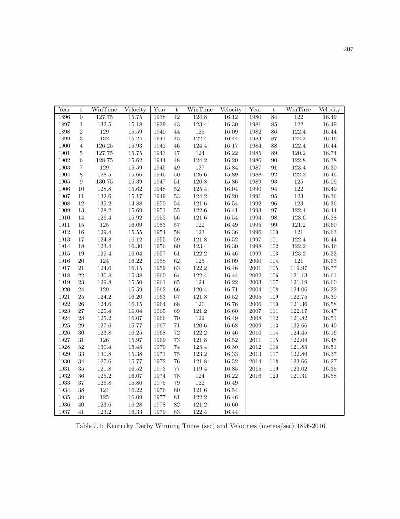
207
Year t WinTime Velocity Year t WinTime Velocity Year t WinTime Velocity
1896 0 127.75 15.75 1938 42 124.8 16.12 1980 84 122 16.491897 1 132.5 15.18 1939 43 123.4 16.30 1981 85 122 16.491898 2 129 15.59 1940 44 125 16.09 1982 86 122.4 16.441899 3 132 15.24 1941 45 122.4 16.44 1983 87 122.2 16.461900 4 126.25 15.93 1942 46 124.4 16.17 1984 88 122.4 16.441901 5 127.75 15.75 1943 47 124 16.22 1985 89 120.2 16.741902 6 128.75 15.62 1944 48 124.2 16.20 1986 90 122.8 16.381903 7 129 15.59 1945 49 127 15.84 1987 91 123.4 16.301904 8 128.5 15.66 1946 50 126.6 15.89 1988 92 122.2 16.461905 9 130.75 15.39 1947 51 126.8 15.86 1989 93 125 16.091906 10 128.8 15.62 1948 52 125.4 16.04 1990 94 122 16.491907 11 132.6 15.17 1949 53 124.2 16.20 1991 95 123 16.361908 12 135.2 14.88 1950 54 121.6 16.54 1992 96 123 16.361909 13 128.2 15.69 1951 55 122.6 16.41 1993 97 122.4 16.441910 14 126.4 15.92 1952 56 121.6 16.54 1994 98 123.6 16.281911 15 125 16.09 1953 57 122 16.49 1995 99 121.2 16.601912 16 129.4 15.55 1954 58 123 16.36 1996 100 121 16.631913 17 124.8 16.12 1955 59 121.8 16.52 1997 101 122.4 16.441914 18 123.4 16.30 1956 60 123.4 16.30 1998 102 122.2 16.461915 19 125.4 16.04 1957 61 122.2 16.46 1999 103 123.2 16.331916 20 124 16.22 1958 62 125 16.09 2000 104 121 16.631917 21 124.6 16.15 1959 63 122.2 16.46 2001 105 119.97 16.771918 22 130.8 15.38 1960 64 122.4 16.44 2002 106 121.13 16.611919 23 129.8 15.50 1961 65 124 16.22 2003 107 121.19 16.601920 24 129 15.59 1962 66 120.4 16.71 2004 108 124.06 16.221921 25 124.2 16.20 1963 67 121.8 16.52 2005 109 122.75 16.391922 26 124.6 16.15 1964 68 120 16.76 2006 110 121.36 16.581923 27 125.4 16.04 1965 69 121.2 16.60 2007 111 122.17 16.471924 28 125.2 16.07 1966 70 122 16.49 2008 112 121.82 16.511925 29 127.6 15.77 1967 71 120.6 16.68 2009 113 122.66 16.401926 30 123.8 16.25 1968 72 122.2 16.46 2010 114 124.45 16.161927 31 126 15.97 1969 73 121.8 16.52 2011 115 122.04 16.481928 32 130.4 15.43 1970 74 123.4 16.30 2012 116 121.83 16.511929 33 130.8 15.38 1971 75 123.2 16.33 2013 117 122.89 16.371930 34 127.6 15.77 1972 76 121.8 16.52 2014 118 123.66 16.271931 35 121.8 16.52 1973 77 119.4 16.85 2015 119 123.02 16.351932 36 125.2 16.07 1974 78 124 16.22 2016 120 121.31 16.581933 37 126.8 15.86 1975 79 122 16.491934 38 124 16.22 1976 80 121.6 16.541935 39 125 16.09 1977 81 122.2 16.461936 40 123.6 16.28 1978 82 121.2 16.601937 41 123.2 16.33 1979 83 122.4 16.44
Table 7.1: Kentucky Derby Winning Times (sec) and Velocities (meters/sec) 1896-2016

208 CHAPTER 7. NONLINEAR REGRESSION
asymptotes. Finally, β4 is the year when the curve is steepest, as well as half way between the lower andupper asymptotes. Here we consider the winning speeds of the Kentucky Derby for years 1896-2016, all yearsthat the horse race was run at a distance of 1.25 miles. The variable t represents Year - 1896, so that the“origin” is the first year the race was 1.25 miles long. For this model, we have:
g (x′t,β) = β1 + (β2 − β1))
[
exp β3 (t− β4)1 + exp β3 (t− β4)
]
∂g (x′t,β)
∂β′ =[
∂g(x′t,β)
∂β1
∂g(x′t,β)
∂β2
∂g(x′t,β)
∂β3
∂g(x′t,β)
∂β4
]
∂g (x′t,β)
∂β1= 1 −
[
exp β3 (t− β4)1 + exp β3 (t− β4)
]
∂g (x′t,β)
∂β2=
[
exp β3 (t − β4)1 + exp β3 (t− β4)
]
∂g (x′t,β)
∂β3= (β2 − β1))
[
(1 + exp β3 (t− β4)) (t− β4) exp β3 (t− β4) − (t− β4) (exp β3 (t− β4))2
(1 + exp β3 (t− β4))2
]
= (β2 − β1)) (t− β4)
[
exp β3 (t − β4)(1 + exp β3 (t− β4))2
]
∂g (x′t,β)
∂β4= (β2 − β1))
[
(1 + exp β3 (t − β4)) (−β3) exp β3 (t− β4) − (−β3) (exp β3 (t− β4))2
(1 + exp β3 (t− β4))2
]
= −β3 (β2 − β1))
[
exp β3 (t − β4)(1 + exp β3 (t− β4))2
]
When choosing starting values for the parameters, it is helpful to think of their effects on predicted valuesin terms of sign and magnitude. For this example, β1 and β2 represent the lower and upper asymptotesof the speeds. Also they enter the equation in a linear form, so that they do not have large effects on theestimation process (as long as β2 > β1). As all races have Velocities between 10 and 20 meters per second,we will start with these values for β1 and β2, respectively. The parameter β4 represents the steepest point

209
of the curve in terms of the year, we will choose the “middle” year, 60. Finally, β3 represents the steepnessof the curve. Suppose we hypothesize that the points that correspond to being 25% and 75% between thelower and upper asymptotes are k years below and above β4, respectively.
⇒ .25 =exp β3 (t.25 − β4)
1 + exp β3 (t.25 − β4)=
exp β3(−k)1 + exp β3(−k)
⇒ β3 =− ln((1/0.25)− 1)
−k =− ln(3)
−k
If we choose k = 20 as a reasonable possibility, it leads to a starting value for β3 = 0.05. We used 0.10in the following program. Note that when using built-in nonlinear regression software procedures in R, SAS,SPSS, and STATA, it is not necessary to be so precise for starting values. However, in many exponentialgrowth and decay models, there are multiple parameterizations of the same function, and if a sign is wrong,or orders of magnitude are incorrect, these programs will not converge.
A set of R commands in matrix form are given below, along with the first two and last two iteratedestimates of β and all inferences regarding β. The variables Year125,...,Speed125 are all based on the yearswhen the race was 1.25 miles (1896-2016).
### Program
kd <- read.csv("http://www.stat.ufl.edu/~winner/data/kentuckyderby.csv",
header=TRUE)
attach(kd); names(kd)
Year125 <- Year[Length==1.25]
Time125 <- Time[Length==1.25]
Length125 <- Length[Length==1.25]
Year125.0 <- Year125-min(Year125)
Speed125 <- 1609.34*Length125/Time125
summary(Speed125)
### Matrix form for logistic model
Y <- Speed125
X.t <- Year125.0
beta.old <- c(10,20,0.1,60)
diff.beta <- 1000
while (diff.beta > .00001)
exp.t <- exp(beta.old[3] * (X.t - beta.old[4]))
G1 <- 1 - (exp.t/(1+exp.t))
G2 <- exp.t/(1+exp.t)
G3 <- (beta.old[2]-beta.old[1]) * (X.t-beta.old[4]) * (exp.t/(1+exp.t)^2)
G4 <- (beta.old[2]-beta.old[1]) * (-beta.old[3]) * (exp.t/(1+exp.t)^2)
G <- cbind(G1,G2,G3,G4)
Yhat <- beta.old[1] + (beta.old[2]-beta.old[1]) * (exp.t/(1+exp.t))
e <- Y - Yhat
beta.new <- beta.old + solve(t(G) %*% G) %*% t(G) %*% e
print(beta.new)
diff.beta <- sum((beta.new-beta.old)^2)
beta.old <- beta.new
exp.t <- exp(beta.old[3] * (X.t - beta.old[4]))
G1 <- 1 - (exp.t/(1+exp.t))
G2 <- exp.t/(1+exp.t)
G3 <- (beta.old[2]-beta.old[1]) * (X.t-beta.old[4]) * (exp.t/(1+exp.t)^2)
G4 <- (beta.old[2]-beta.old[1]) * (-beta.old[3]) * (exp.t/(1+exp.t)^2)
G <- cbind(G1,G2,G3,G4)
Yhat <- beta.old[1] + (beta.old[2]-beta.old[1]) * (exp.t/(1+exp.t))

210 CHAPTER 7. NONLINEAR REGRESSION
e <- Y - Yhat
(SSE <- t(e) %*% e)
(MSE <- SSE/(length(Y) - ncol(G)))
V.beta <- MSE[1,1] * solve(t(G) %*% G)
SE.beta <- sqrt(diag(V.beta))
t.beta <- beta.new/SE.beta
P.beta <- 2*(1-pt(abs(t.beta),length(Y)-ncol(G)))
print(round(cbind(beta.new,SE.beta,t.beta,P.beta),4))
(CI.beta1 <- beta.new[1] + qt(c(.025,.975),length(Y)-ncol(G))*SE.beta[1])
(CI.beta2 <- beta.new[2] + qt(c(.025,.975),length(Y)-ncol(G))*SE.beta[2])
(CI.beta3 <- beta.new[3] + qt(c(.025,.975),length(Y)-ncol(G))*SE.beta[3])
(CI.beta4 <- beta.new[4] + qt(c(.025,.975),length(Y)-ncol(G))*SE.beta[4])
### Output
> Speed125 <- 1609.34*Length125/Time125
> summary(Speed125)
Min. 1st Qu. Median Mean 3rd Qu. Max.
14.88 16.04 16.30 16.20 16.49 16.85
[,1]
G1 15.69133064
G2 16.47338070
G3 0.09592648
G4 58.53688771
[,1]
G1 15.67313699
G2 16.47186534
G3 0.05280251
G4 39.73971423
...
[,1]
G1 15.36095708
G2 16.48585093
G3 0.06381906
G4 27.58451474
[,1]
G1 15.3609265
G2 16.4858482
G3 0.0638184
G4 27.5832162
> (SSE <- t(e) %*% e)
[,1]
[1,] 6.607435
> (MSE <- SSE/(length(Y) - ncol(G)))
[,1]
[1,] 0.0564738
> print(round(cbind(beta.new,SE.beta,t.beta,P.beta),4))
SE.beta
G1 15.3609 0.2823 54.4092 0.0000
G2 16.4858 0.0464 355.3788 0.0000
G3 0.0638 0.0230 2.7781 0.0064
G4 27.5832 9.2703 2.9755 0.0036
> (CI.beta1 <- beta.new[1] + qt(c(.025,.975),length(Y)-ncol(G))*SE.beta[1])
[1] 14.80180 15.92005
> (CI.beta2 <- beta.new[2] + qt(c(.025,.975),length(Y)-ncol(G))*SE.beta[2])
[1] 16.39398 16.57772
> (CI.beta3 <- beta.new[3] + qt(c(.025,.975),length(Y)-ncol(G))*SE.beta[3])
[1] 0.01832384 0.10931295
> (CI.beta4 <- beta.new[4] + qt(c(.025,.975),length(Y)-ncol(G))*SE.beta[4])
[1] 9.223954 45.942479

211
The analysis based on the nls function is given below. Note that we don’t need to be so precise onstarting values, due to the algorithm used in computations. A plot of the data and the fitted regressionequation is given in Figure 7.1. A plot of Residuals versus Year does demonstrate higher variance in earlyyears then in later years, but the difference is not very drastic. It could very well be due to less accuratetiming equipment. The residual plot is given in Figure 7.2.
R Program
kd <- read.csv("http://www.stat.ufl.edu/~winner/data/kentuckyderby.csv",
header=TRUE)
attach(kd); names(kd)
Year125 <- Year[Length==1.25]
Time125 <- Time[Length==1.25]
Length125 <- Length[Length==1.25]
Year125.0 <- Year125-min(Year125)
Speed125 <- 1609.34*Length125/Time125
summary(Speed125)
Speed125.2008 <- Speed125[Year125<=2008]
Year125.2008 <- Year125[Year125<=2008]
kd.mod1 <- nls(Speed125 ~ b0 + (b1-b0)*exp(b2*(Year125.0-b3))/
(1+exp(b2*(Year125.0-b3))), start=c(b0=1,b1=20,b2=1,b3=60))
summary(kd.mod1)
AIC(kd.mod1)
confint(kd.mod1)
plot(Year125.0,Speed125)
lines(Year125.0,predict(kd.mod1,Year125))
R Output
Formula: Speed125 ~ b0 + (b1 - b0) * exp(b2 * (Year125.0 - b3))/(1 + exp(b2 *
(Year125.0 - b3)))
Parameters:
Estimate Std. Error t value Pr(>|t|)
b0 15.36090 0.28235 54.404 < 2e-16 ***
b1 16.48585 0.04639 355.369 < 2e-16 ***
b2 0.06382 0.02297 2.778 0.00637 **
b3 27.58248 9.27100 2.975 0.00356 **
Residual standard error: 0.2376 on 117 degrees of freedom
Number of iterations to convergence: 17
Achieved convergence tolerance: 8.259e-06
> AIC(kd.mod1)
[1] 1.564131
> confint(kd.mod1)
Waiting for profiling to be done...
Error in prof$getProfile() : number of iterations exceeded maximum of 50
∇

212 CHAPTER 7. NONLINEAR REGRESSION
0 20 40 60 80 100 120
15.0
15.5
16.0
16.5
Year125.0
Speed125
Figure 7.1: Kentucky Derby Winning Velocities and Fitted Logistic Function - 1896-2016
0 20 40 60 80 100 120
−0.8
−0.6
−0.4
−0.2
0.0
0.2
0.4
Year125.0
resid
(kd.m
od1)
Figure 7.2: Kentucky Derby Residuals versus Year - 1896-2016

213
For linear functions of β of the form K′β, we then have approximate normality of the estimator K′β:
K′βapprox∼ N
(
K′β, σ2K′ (G′G)−1
K)
Thus, to test H0 : K′β = m, where K′ has q linearly independent rows (restrictions on the regressioncoefficients), we have the following test statistic and rejection region.
TS : Fobs =
(
K′β −m)′[
K′(
G′G)−1
K
]−1(
K′β −m)
qs2RR : Fobs ≥ Fq,n−p
with an approximate P -value as the area above the test statistic Fobs for the Fq,n−p distribution.
Example: Beer Foam Heights Over Time for 3 Beer Brands
Leike (2002) reported results of an experiment measuring beer foam height over a 6 minute period for3 brands of beer (Erdinger Weissbier, Augustinerbrau Munchen, and Budweiser). The data are given inTable 7.2. There are a total of n = 3(15) = 45 observations when we “stack” the data for 3 brands. Anexponential decay model with additive errors is fit, allowing for different curves for the 3 brands, with trepresenting time, and dummy variables: Xi1 = 1 if Erdinger, 0 otherwise; Xi2 = 1 if Augustinerbrau, 0otherwise; and Xi3 = 1 if Budweiser, 0 otherwise.
Yi = β01Xi1 exp−β11Xi1ti + β02Xi2 exp−β12Xi2ti + β03Xi3 exp−β13Xi3ti + εi i = 1, . . . , 45
The R program and output are given below. Note that the algorithm fails when ti = 0, so replace itwith ti = 0.0001. A plot of the data and the fitted curves are given in Figure 7.3.
R Program
beerfoam <- read.table("http://www.stat.ufl.edu/~winner/data/beer_foam2.dat",
header=F,col.names=c("foam.time","brand1","brand2","brand3"))
attach(beerfoam)
foam.time
for (i in 1:length(foam.time))
if (foam.time[i] == 0) foam.time[i] <- 0.0001
foam.time
Y.foam <- c(brand1,brand2,brand3)
X1 <- c(rep(1,15),rep(0,15),rep(0,15))
X2 <- c(rep(0,15),rep(1,15),rep(0,15))
X3 <- c(rep(0,15),rep(0,15),rep(1,15))
t.foam <- c(foam.time,foam.time,foam.time)
brand <- rep(1:3,each=15)
foam.mod1 <- nls(Y.foam ~ b01*X1*exp(-b11*X1*t.foam) +
b02*X2*exp(-b12*X2*t.foam) + b03*X3*exp(-b13*X3*t.foam),
start=c(b01=10,b02=10,b03=10,b11=0.01,b12=0.01,b13=0.01))
summary(foam.mod1)
time.x <- 0:360

214 CHAPTER 7. NONLINEAR REGRESSION
Time (sec) Erdinger Augustinerbrau Budweiser
0 17.0 14.0 14.015 16.1 11.8 12.130 14.9 10.5 10.945 14.0 9.3 10.060 13.2 8.5 9.375 12.5 7.7 8.690 11.9 7.1 8.0105 11.2 6.5 7.5120 10.7 6.0 7.0150 9.7 5.3 6.2180 8.9 4.4 5.5210 8.3 3.5 4.5240 7.5 2.9 3.5300 6.3 1.3 2.0360 5.2 0.7 0.9
Table 7.2: Beer Foam Heights for 3 Brands of Beer over Time
yhat.b1 <- coef(foam.mod1)[1] * exp(-coef(foam.mod1)[4]*time.x)
yhat.b2 <- coef(foam.mod1)[2] * exp(-coef(foam.mod1)[5]*time.x)
yhat.b3 <- coef(foam.mod1)[3] * exp(-coef(foam.mod1)[6]*time.x)
plot(t.foam,Y.foam,pch=brand)
lines(time.x,yhat.b1,lty=1)
lines(time.x,yhat.b2,lty=2)
lines(time.x,yhat.b3,lty=5)
legend(240,16,c("Erd","Aug","Bud"),pch=c(1,2,3),lty=c(1,2,5))
R Output
> summary(foam.mod1)
Formula: Y.foam ~ b01 * X1 * exp(-b11 * X1 * t.foam) + b02 * X2 * exp(-b12 *
X2 * t.foam) + b03 * X3 * exp(-b13 * X3 * t.foam)
Parameters:
Estimate Std. Error t value Pr(>|t|)
b01 1.650e+01 2.080e-01 79.32 <2e-16 ***
b02 1.323e+01 2.469e-01 53.61 <2e-16 ***
b03 1.337e+01 2.346e-01 57.02 <2e-16 ***
b11 3.396e-03 1.172e-04 28.98 <2e-16 ***
b12 6.758e-03 2.534e-04 26.67 <2e-16 ***
b13 5.625e-03 2.117e-04 26.57 <2e-16 ***
Residual standard error: 0.3931 on 39 degrees of freedom
Number of iterations to convergence: 6
Achieved convergence tolerance: 4.779e-07
We test whether the curves for Augustinerbrau and Budweiser are the same. This can be conductedbased on the matrix form described above, as well as by fitting a Reduced Model and comparing it with thecomplete model. What is being tested is as follows.

215
0 50 100 150 200 250 300 350
510
15
t.foam
Y.foam
Erd
Aug
Bud
Figure 7.3: Plot of Beer Foam versus Time and Brand Specific Fitted Equations
H0 : β02 = β03, β12 = β13 ⇒ K′β = 0 K′ =
[
0 1 −1 0 0 00 0 0 0 1 −1
]
β =
β01
β02
β03
β11
β12
β13
In R, the object produced by many regression functions including lm and nls contains many itemsthat can be “selected” from the object. Relevant to this test, we can obtain: β as coef(foam.mod1),
SSE as deviance(foam.mod1), and V β = s2(
G′G)−1
as vcov(foam.mod1). Then we can isolate(
G′G)−1
by dividing the estimated variance-covariance of β by s2 = MSE = SSE/(n − p). The following
R commands, run after fitting foam.mod1 above, will conduct the F -test.
### Commands
(beta.foam1 <- coef(foam.mod1))
vcov.foam1 <- vcov(foam.mod1)
(mse <- deviance(foam.mod1)/(45-6))
GpGinv <- vcov.foam1/mse
Kp <- matrix(c(0,1,-1,0,0,0,0,0,0,0,1,-1),byrow=T,ncol=6)
(F.foam1a <- t(Kp %*% beta.foam1) %*% solve(Kp %*% GpGinv %*% t(Kp)) %*%
(Kp %*% beta.foam1))

216 CHAPTER 7. NONLINEAR REGRESSION
(F.foam1b <- nrow(Kp)*mse)
(F.foam1 <- F.foam1a / F.foam1b)
(crit.F <- qf(.95,2,39))
(P.F <- 1-pf(F.foam1,2,39))
### Output
> (beta.foam1 <- coef(foam.mod1))
b01 b02 b03 b11 b12 b13
16.495318508 13.233329203 13.373355980 0.003396205 0.006757962 0.005625264
> (mse <- deviance(foam.mod1)/(45-6))
[1] 0.1545567
> Kp <- matrix(c(0,1,-1,0,0,0,0,0,0,0,1,-1),byrow=T,ncol=6)
> (F.foam1a <- t(Kp %*% beta.foam1) %*% solve(Kp %*% GpGinv %*% t(Kp)) %*%
+ (Kp %*% beta.foam1))
[1,] 4.186677
> (F.foam1b <- nrow(Kp)*mse)
[1] 0.3091133
> (F.foam1 <- F.foam1a / F.foam1b)
[1,] 13.54415
> (crit.F <- qf(.95,2,39))
[1] 3.238096
> (P.F <- 1-pf(F.foam1,2,39))
[1,] 3.414526e-05
We strongly reject the hypothesis that the curves are the same for Augustinerbrau and Budweiser. Thesecond approach involves “forcing” β02 = β03 and β12 = β13 and fitting the ensuing model. This is done asfollows.
X23 = X2 +X3 Yi = β01Xi1 exp−β11Xi1ti + β023Xi23 exp−β123Xi23ti + εi
The R Program and Output are given below.
R Program
### Fit Reduced Model
X23 <- X2 + X3
foam.mod2 <- nls(Y.foam ~ b01*X1*exp(-b11*X1*t.foam) +
b023*X23*exp(-b123*X23*t.foam),
start=c(b01=10,b023=10,b11=0.01,b123=0.01))
summary(foam.mod2)
### Compare Reduced and Complete Models
anova(foam.mod2,foam.mod1)
R Output
> summary(foam.mod2)
Formula: Y.foam ~ b01 * X1 * exp(-b11 * X1 * t.foam) + b023 * X23 * exp(-b123 *
X23 * t.foam)
Parameters:

217
Estimate Std. Error t value Pr(>|t|)
b01 1.650e+01 2.652e-01 62.20 <2e-16 ***
b023 1.329e+01 2.167e-01 61.30 <2e-16 ***
b11 3.396e-03 1.494e-04 22.73 <2e-16 ***
b123 6.148e-03 2.082e-04 29.53 <2e-16 ***
Residual standard error: 0.5014 on 41 degrees of freedom
Number of iterations to convergence: 6
Achieved convergence tolerance: 3.585e-07
>
> anova(foam.mod2,foam.mod1)
Analysis of Variance Table
Model 1: Y.foam ~ b01 * X1 * exp(-b11 * X1 * t.foam) + b023 * X23 * exp(-b123 * X23 * t.foam)
Model 2: Y.foam ~ b01 * X1 * exp(-b11 * X1 * t.foam) + b02 * X2 * exp(-b12 * X2 * t.foam) +
b03 * X3 * exp(-b13 * X3 * t.foam)
Res.Df Res.Sum Sq Df Sum Sq F value Pr(>F)
1 41 10.3060
2 39 6.0277 2 4.2783 13.841 2.869e-05 ***
Note that the matrix form and the Complete versus Reduced form give slightly different F -statistics.The equivalency derived in the case of linear regression does not hold in the case of nonlinear regression.
∇
By the nature of nonlinear models, we may also be interested in nonlinear functions of the parameters,
say h (β), which cannot be written in the form K′β. In this case, the estimator h(
β)
is approximately
normally distributed:
h(
β)
approx∼ N(
h (β) , σ2(
H (G′G)−1
H′))
where
H (β) =
[
∂h(β)∂β1
∂h(β)∂β2
· · · ∂h(β)∂β
p
]
.
The estimated variance of h(
β)
replaces both H and G with their estimates, replacing β with β. Estimates
(Confidence Intervals) and tests concerning h (β) can be obtained as follow.
(1−α)100% CI for h (β) : h(
β)
±t (α/2, n− p) SE
h(
β) h
(
β)
− h0
SE
h(
β)
approx∼ tn−p Under H0 : h (β) = h0
where:
SE
h(
β)
=
√
s2H(
G′G)−1
H′.
When there are several (q) nonlinear functions, an approximate Wald test of h (β) = h0 is:
TS : Fobs =
(
h(
β)
− h0
)′[
H(
G′G)−1
H′
]−1(
h(
β)
− h0
)
qs2RR : W ≥ Fq,n−p

218 CHAPTER 7. NONLINEAR REGRESSION
with P -value being the upper-tail area above Fobs for the Fq,n−p distribution. Here, we define:
h (β) =
h1 (β)h2 (β)
...hq (β)
H (β) =
∂h1(β)∂β1
∂h1(β)∂β2
· · · ∂h1(β)∂β
p
∂h2(β)∂β1
∂h2(β)∂β2
· · · ∂h2(β)∂β
p
......
. . ....
∂hq(β)∂β
1
∂hq(β)∂β
2
· · · ∂hq(β)∂β
p
Example: Winning Velocities and Completion Times in the Kentucky Derby
Suppose we are interested in the “percentage change” in mean velocity in horses, based on the KentuckyDerby data. Recall that β1 is the lower asymptote and β2 is the upper asymptote. Then, we are interestedin the following nonlinear function of the coefficient vector β.
h (β) = 100
(
β2 − β1
β1
)
⇒ ∂h (β)
∂β1
=−100β2
β21
∂h (β)
∂β2
=100
β1
From the model fit previously, we have the following estimates.
β1 = 15.36090 β2 = 16.48586 s = 0.2376 s2 = 0.056454
⇒ h(
β)
= 100
(
16.48586− 15.36090
15.36090
)
= 7.32353 H(
β)
=[
−6.98680 6.51004 0 0]
The R Commands and Output to compute a 95% Confidence Interval for h (β) are given below.
### Commands
### Matrix form for logistic model
Y <- Speed125
X.t <- Year125.0
beta.old <- c(10,20,0.1,60)
diff.beta <- 1000
while (diff.beta > .00001)
exp.t <- exp(beta.old[3] * (X.t - beta.old[4]))
G1 <- 1 - (exp.t/(1+exp.t))
G2 <- exp.t/(1+exp.t)
G3 <- (beta.old[2]-beta.old[1]) * (X.t-beta.old[4]) * (exp.t/(1+exp.t)^2)
G4 <- (beta.old[2]-beta.old[1]) * (-beta.old[3]) * (exp.t/(1+exp.t)^2)
G <- cbind(G1,G2,G3,G4)
Yhat <- beta.old[1] + (beta.old[2]-beta.old[1]) * (exp.t/(1+exp.t))
e <- Y - Yhat
beta.new <- beta.old + solve(t(G) %*% G) %*% t(G) %*% e

219
print(beta.new)
diff.beta <- sum((beta.new-beta.old)^2)
beta.old <- beta.new
exp.t <- exp(beta.old[3] * (X.t - beta.old[4]))
G1 <- 1 - (exp.t/(1+exp.t))
G2 <- exp.t/(1+exp.t)
G3 <- (beta.old[2]-beta.old[1]) * (X.t-beta.old[4]) * (exp.t/(1+exp.t)^2)
G4 <- (beta.old[2]-beta.old[1]) * (-beta.old[3]) * (exp.t/(1+exp.t)^2)
G <- cbind(G1,G2,G3,G4)
Yhat <- beta.old[1] + (beta.old[2]-beta.old[1]) * (exp.t/(1+exp.t))
e <- Y - Yhat
(SSE <- t(e) %*% e)
(MSE <- SSE/(length(Y) - ncol(G)))
(h.beta <- 100*(beta.old[2]-beta.old[1]) / beta.old[1])
(H.beta1 <- -100*beta.old[2]/(beta.old[1]^2))
(H.beta2 <- 100/beta.old[1])
H.beta3 <- 0; H.beta4 <- 0
H.beta <- cbind(H.beta1,H.beta2,H.beta3,H.beta4)
(SE.h.beta <- sqrt(MSE[1,1] * (H.beta %*% solve(t(G) %*% G) %*% t(H.beta))))
(CI.h.beta <- h.beta + qt(c(.025,.975),length(Y)-ncol(G))*SE.h.beta)
### Output
> (SSE <- t(e) %*% e)
[1,] 6.607435
> (MSE <- SSE/(length(Y) - ncol(G)))
[1,] 0.0564738
> (h.beta <- 100*(beta.old[2]-beta.old[1]) / beta.old[1])
[1] 7.323268
> (H.beta1 <- -100*beta.old[2]/(beta.old[1]^2))
[1] -6.98677
> (H.beta2 <- 100/beta.old[1])
[1] 6.510024
> H.beta3 <- 0; H.beta4 <- 0
> H.beta <- cbind(H.beta1,H.beta2,H.beta3,H.beta4)
> (SE.h.beta <- sqrt(MSE[1,1] * (H.beta %*% solve(t(G) %*% G) %*% t(H.beta))))
[1,] 2.136145
> (CI.h.beta <- h.beta + qt(c(.025,.975),length(Y)-ncol(G))*SE.h.beta)
[1] 3.092744 11.553791
∇
When the error variance is not constant, we can fit estimated weighted NLS. The weights would be theinverse of the estimated variances, as in the case of Linear Regression described previously. The variancesmay be related to the mean and/or the levels of one or more predictor variables. This will necessarily be aniterative process. The function we want to minimize is:
QW =
n∑
i=1
[v (g (x′i; β))]
−1[Yi − g (x′
i; β)]2
where σ2i = v (g (x′
i; β)) .
When there are replicates at distinct X levels, we can use the estimated variances of the replicates as theweights, in a manner like that used for the Shotgun spread example previously.
Example: Experiments in Salmonella Growth

220 CHAPTER 7. NONLINEAR REGRESSION
Alvord, et al (1990) report growth of salmonella as a nonlinear function of mutagen dose over twoexperimental days. We consider the data from the second experimental day, with 3 replicates at each of 7doses, with n = 21. The data are given in Table 7.3, along with the dose specific sample standard deviations.A plot of the data and the subsequent fitted equation is given in Figure 7.4. The authors fit the followingnonlinear model, where Y is the number of colonies observed, and X is the dose. The weights are the inversevariance for the various doses.
Yi = [β0 + expβ1 + β2 lnXi] exp−β3Xi + εi i = 1, . . . , 21
The R Program and Output are given below. The data and fitted equation is given in Figure 7.4.
R Program
salmonella <- read.table("http://www.stat.ufl.edu/~winner/data/salmonella.dat",header=F,
col.names=c("expt","dose","colonies"))
attach(salmonella)
for (i in 1:length(dose)) if(dose[i] == 0) dose[i] <- 0.000001
expt01 <- expt-1
(vardoseexp <- aggregate(colonies,by=list(dose,expt),FUN=var))
(ndoseexp <- aggregate(colonies,by=list(dose,expt),FUN=length))
(varwt <- rep(1/vardoseexp[[3]],each=ndoseexp[[3]]))
salmonella <- data.frame(salmonella,varwt)
expt1 <- subset(salmonella,expt==1)
expt2 <- subset(salmonella,expt==2)
plot(dose,colonies,data=expt2)
salm.mod2 <- nls(colonies ~ (b0+exp(b1+b2*log(dose)))*exp(-b3*dose),
start=c(b0=20,b1=10,b2=1,b3=1),weight=varwt,data=expt2)
summary(salm.mod2)
deviance(salm.mod2)
plot(dose,colonies,data=expt2)
dosev <- seq(.001,3.200,.001)
yhatexp2 <- predict(salm.mod2,list(dose=dosev))
lines(dosev,yhatexp2,lty=1)
R Output
> summary(salm.mod2)
Formula: colonies ~ (b0 + exp(b1 + b2 * log(dose))) * exp(-b3 * dose)
Parameters:
Estimate Std. Error t value Pr(>|t|)
b0 21.19355 2.52609 8.390 1.90e-07 ***
b1 7.26329 0.04514 160.891 < 2e-16 ***
b2 1.20024 0.05033 23.846 1.66e-14 ***
b3 0.30620 0.03571 8.574 1.40e-07 ***
Residual standard error: 0.9569 on 17 degrees of freedom

221
Experiment Dose Colonies SD.Dose Experiment Dose Colonies SD.Dose
2 0 17 4.582576 1 0 25 4.3588992 0 26 4.582576 1 0 18 4.3588992 0 20 4.582576 1 0 26 4.3588992 0.1 147 28.05352 1 0.1 156 7.5055532 0.1 91 28.05352 1 0.1 149 7.5055532 0.1 116 28.05352 1 0.1 164 7.5055532 0.2 223 21.37756 1 0.2 294 29.569132 0.2 192 21.37756 1 0.2 268 29.569132 0.2 233 21.37756 1 0.2 327 29.569132 0.4 373 46.04708 1 0.4 511 19.553352 0.4 462 46.04708 1 0.4 473 19.553352 0.4 438 46.04708 1 0.4 500 19.553352 0.8 848 19.2873 1 0.8 1017 46.436342 0.8 878 19.2873 1 0.8 925 46.436342 0.8 884 19.2873 1 0.8 960 46.436342 1.6 1796 147.6347 1 1.6 1432 60.224582 1.6 1552 147.6347 1 1.6 1363 60.224582 1.6 1530 147.6347 1 1.6 1483 60.224582 3.2 2187 126.4608 1 3.2 1890 48.603842 3.2 2020 126.4608 1 3.2 1868 48.603842 3.2 2268 126.4608 1 3.2 1961 48.60384
Table 7.3: Salmonella Colonies Observed and Mutagen Dose for Experiments 2 and 1
Number of iterations to convergence: 8
Achieved convergence tolerance: 6.668e-07
> deviance(salm.mod2)
[1] 15.56472
A series of models were fit for both experimental days. Let Xi1 be the dose, and Xi2 be 1 for experiment2, and 0 for experiment 1. Now there are n = 42 total measurements. The models are as follow.
M3: Yi = Xi2 [β0 + expβ1 + β2 lnXi1] exp−β3Xi1+(1 −Xi2) [β0 + expβ1 + β2 lnXi1] exp−β3Xi1+εi
M4: Yi = Xi2 [β02 + expβ12 + β22 lnXi1] exp−β32Xi1+(1 −Xi2) [β01 + expβ11 + β21 lnXi1] exp−β31Xi1+εiM5: Yi = Xi2 [β02 + expβ1 + β22 lnXi1] exp−β3Xi1+(1 −Xi2) [β01 + expβ1 + β21 lnXi1] exp−β3Xi1+εiM6: Yi = Xi2 [β0 + expβ1 + β22 lnXi1] exp−β3Xi1+(1 −Xi2) [β0 + expβ1 + β21 lnXi1] exp−β3Xi1+εiM7: Yi = Xi2 [β02 + expβ1 + β2 lnXi1] exp−β3Xi1+(1 −Xi2) [β01 + expβ1 + β2 lnXi1] exp−β3Xi1+εiM8: Yi = Xi2 [β0 + expβ12 + β2 lnXi1] exp−β3Xi1+(1 −Xi2) [β0 + expβ11 + β2 lnXi1] exp−β3Xi1+εiM9: Yi = Xi2 [β02 + expβ1 + β2 lnXi1] exp−β32Xi1+(1 −Xi2) [β01 + expβ1 + β2 lnXi1] exp−β31Xi1+εi
A portion of the R Program and Output are given below, and summaries of the models are given inTable 7.4. A plot of the data and the regression based on Model 4 is given in Figure 7.5. The ResidualStandard Error is based on the weighted residuals, not the “true” residuals. Note that the R functionsdeviance, logLik, and AIC do not work correctly for the nls function when the weight option is used.

222 CHAPTER 7. NONLINEAR REGRESSION
0.0 0.5 1.0 1.5 2.0 2.5 3.0
0500
1000
1500
2000
dose[expt == 2]
colo
nie
s[e
xpt =
= 2
]
Figure 7.4: Plot of Colonies and Fitted Equation for Experiment 2
We computed SSE, AIC, and BIC directly. AIC and BIC are computed as a multiplier of the number ofetimated parameters (including σ2) - twice the log-likelihood evaluated at the ML estimates for µ and σ2.
SSE =n∑
i=1
(
Yi − Yi
)2
AIC = 2(p+ 1) + n
[
ln(2π) + ln
(
SSE
n
)
+ 1
]
BIC = ln(n)(p+ 1) + n
[
ln(2π) + ln
(
SSE
n
)
+ 1
]
salm.mod4 <- nls(colonies ~ expt01*(b02+exp(b12+b22*log(dose)))*exp(-b32*dose)
+ (1-expt01)*(b01+exp(b11+b21*log(dose)))*exp(-b31*dose),
start=c(b01=20,b11=10,b21=1,b31=1,b02=20,b12=10,b22=1,b32=1),
weight=varwt,data=salmonella)
summary(salm.mod4)
deviance(salm.mod4)
AIC(salm.mod4)
plot(dose,colonies,pch=expt)
dosev <- seq(.001,3.200,.001)
expt1v <- rep(0,length(seq(.001,3.200,.001)))
expt2v <- rep(1,length(seq(.001,3.200,.001)))
yhatexp1 <- predict(salm.mod6,list(dose=dosev, expt01=expt1v))
yhatexp2 <- predict(salm.mod6,list(dose=dosev, expt01=expt2v))

223
Model SSE AIC BIC Parameters
3 399778.5 513.9527 522.6410 4+1=54 136627.4 476.8593 492.4983 8+1=95 155795.1 478.3732 490.5369 6+1=76 160459.2 477.6121 488.0381 5+1=67 394878.6 515.4347 525.8607 5+1=68 490021.1 524.5013 534.9273 5+1=69 219897.4 492.8472 505.0109 6+1=7
Table 7.4: Model Fit Statistic (Note that # of Parameters includes σ2)
lines(dosev,yhatexp1,lty=1)
lines(dosev,yhatexp2,lty=2)
legend("topleft",c("Experiment1","Experiment2"),pch=c(1,2),lty=c(1,2))
### Output
> summary(salm.mod4)
Formula: colonies ~ expt01 * (b02 + exp(b12 + b22 * log(dose))) * exp(-b32 *
dose) + (1 - expt01) * (b01 + exp(b11 + b21 * log(dose))) *
exp(-b31 * dose)
Parameters:
Estimate Std. Error t value Pr(>|t|)
b01 23.15862 2.67842 8.646 4.21e-10 ***
b11 7.21858 0.03948 182.857 < 2e-16 ***
b21 1.00008 0.02683 37.274 < 2e-16 ***
b31 0.26099 0.02292 11.389 3.77e-13 ***
b02 21.19355 2.82742 7.496 1.06e-08 ***
b12 7.26329 0.05053 143.744 < 2e-16 ***
b22 1.20024 0.05634 21.305 < 2e-16 ***
b32 0.30620 0.03997 7.660 6.64e-09 ***
Residual standard error: 1.071 on 34 degrees of freedom
Number of iterations to convergence: 8
Achieved convergence tolerance: 4.08e-07
> deviance(salm.mod4)
[1] 38.99907
> AIC(salm.mod4)
[1] 11570.38
∇
If the errors are correlated with a known correlation structure, such as AR(1), the autoregressive pa-rameter(s) can be estimated and plugged into the variance-covariance matrix, and we can fit estimatedgeneralized NLS. Here we want to minimize:
[Yi − g (x′i; β)]
′V−1 [Yi − g (x′
i; β)]
where the elements of V are functions of unknown parameters which are estimated from the residuals. Seethe AR(1) description for Linear Regression.

224 CHAPTER 7. NONLINEAR REGRESSION
0.0 0.5 1.0 1.5 2.0 2.5 3.0
0500
1000
1500
2000
dose
colo
nie
s
Experiment1
Experiment2
Figure 7.5: Dose Response Curves Based on Model 6 - Salmonella Experiments

Chapter 8
Random Coefficient RegressionModels
Random coefficient regression (RCR) models are typically longitudinal in nature, with a sample of nunits being observed on multiple occasions, with Y and X1,...,Xp being observed on units at the variousoccasions. These models are widely used in various disciplines, and are also known as Hierarchical LinearModels (HLMs) and Multilevel Models. These methods are described in various books and chapters(e.g. Bryk and Raudenbush (1992), Goldstein (1987), Rawlings, Pantula, and Dickey (1998, Sections 18.3-18.4), and Littell, Milliken, Stroup, and Wolfinger (1996, Chapter 7). Note that nonlinear regression modelscan also have random coefficients. Here we consider a simple, balanced model, then consider more generalcases.
8.1 Balanced Model with 1 Predictor
We consider a case where n experimental units are each observed at t occasion, with observed pairs(Xij , Yij) i = 1, · · · , n; j = 1, ..., t. The model allows for different intercepts and slopes among te units.Note that in many growth curve applications among units, the predictor variable is simply the time point.
Yij = αi + βiXij + εij i = 1, ..., n; j = 1, ..., t εij ∼ N(
0, σ2)
independent
[
αi
βi
]
∼ N
([
αβ
]
,
[
σ2α σαβ
σαβ σ2β
])
ε⊥[
αi
βi
]
An alternative, widely used way to re-write this model is as follows.
Yij = (α+ βXij ) + [(αi − α) + (βi − β)Xij + εij]
⇒ E Yij = α+ βXij V Yij = σ2α +X2
ijσ2β + σ2 + 2Xijσαβ
j 6= j′ : COV Yij, Yij′ = σ2α +XijXij′σ2
β + (Xij +Xij′)σαβ
225

226 CHAPTER 8. RANDOM COEFFICIENT REGRESSION MODELS
8.2 General Model with p Predictors
Gumpertz and Pantula (1989) considered a general (balanced) model, and obtained unbiased estimators ofthe model parameters. When the number of measurements per subject are equal (e.g. balanced model),these “simple” estimators coincide with those obtained from mixed model statistical software proceduresthat perform EGLS estimation of the model parameters. The scalar and matrix forms are given below, alongwith the mean and variance/covariance structure.
Yij = βi0 + βi1Xij1 + · · ·+ βipXijp + εij i = 1, . . . , n; j = 1, . . . , t
Yi = Xiβi + εi Yi =
Yi1
Yi2
...Yit
Xi =
1 Xi11 · · · Xi1p
1 Xi21 · · · Xi2p
......
. . ....
1 Xit1 · · · Xitp
βi =
βi0
βi1
...βip
εi =
εi1εi2...εit
βi ∼ NID (β,Σβ) εi ∼ NID(
0, σ2I)
βi⊥εi
β =
β0
β1
...βp
Σβ =
V βi0 COV βi0, βi1 · · · COV βi0, βipCOV βi0, βi1 V βi1 · · · COV βi1, βip
......
. . ....
COV βi0, βip COV βi1, βip · · · V βip
E Yi = E Xiβi + εi = Xiβ V Yi = V Xiβi + εi = XiΣβX′i+σ
2I COV Yi,Yi′ = 0 i 6= i′
Yi ∼ N(
Xiβ,XiΣβX′i + σ2I
)
The predictor of the ith unit’s regression coefficient vector can be obtained by fitting the regression for thatindividual.
βi = (X′iXi)
−1X′
iYi E
βi
= (X′iXi)
−1X′
iXiβ = β
V
βi
= (X′iXi)
−1X′
i
[
XiΣβX′i + σ2I
]
Xi (X′iXi)
−1= Σβ + σ2 (X′
iXi)−1
Note that each individual’s βi is an unbiased estimator of the population mean β. That leads to makinguse of a simple average of the βi as an unbiased estimator of the mean vector.
β =1
n
n∑
i=1
βi ⇒ E
β
=1
nnβ = β

8.2. GENERAL MODEL WITH P PREDICTORS 227
V
β
=1
n2
[
nΣβ + σ2n∑
i=1
(X′iXi)
−1
]
COV
βi, β
=1
n
[
Σβ + σ2 (X′iXi)
−1]
Now, making use of the distributional properties of the regression model, we can estimate σ2 and Σ.
(
Yi − Xiβi
)′ (
Yi − Xiβi
)
= Y′i (I −Pi)Yi Pi = Xi (X′
iXi)−1
X′i
E Y′i (I −Pi)Yi = σ2trace (I−Pi) + β
′X′i (I −Pi) Xiβ = σ2 (t− p′) + 0
⇒ E
n∑
i=1
(
Yi − Xiβi
)′ (
Yi − Xiβi
)
= n (t− p′)σ2
⇒ s2 =1
n (t− p′)
n∑
i=1
(
Yi − Xiβi
)′ (
Yi −Xiβi
)
=1
n (t− p′)
n∑
i=1
SSEi =1
n
n∑
i=1
MSEi
V
βi − β
= E
(
βi − β)(
βi − β)′
−E(
βi − β)
E
(
βi − β)′
E(
βi − β)
= β−β = 0
⇒ E
(
βi − β)(
βi − β)′
= V
βi − β
= V
βi
+ V
β
− 2COV
βi, β
=
Σβ + σ2 (X′iXi)
−1+
1
n2
[
nΣβ + σ2n∑
i=1
(X′iXi)
−1
]
− 21
n
[
Σβ + σ2 (X′iXi)
−1]
=
n− 1
nΣβ + σ2 (X′
iXi)−1[
1 +1
n2− 2
n
]
+σ2
n2
n∑
j=1j 6=i
(
X′jXj
)−1
⇒ E
n∑
i=1
(
βi − β)(
βi − β)′
= n
(
n− 1
n
)
Σβ+σ2
[
1 +1
n2− 2
n
] n∑
i=1
(X′iXi)
−1+σ2
n2
n∑
i=1
n∑
j=1j 6=i
(
X′jXj
)−1
Note that in the last double summation, each unit (i) appears n− 1 times.
⇒ E
n∑
i=1
(
βi − β)(
βi − β)′
= (n− 1)Σβ + σ2
[
1 +1
n2− 2
n+n− 1
n2
] n∑
i=1
(X′iXi)
−1
= (n− 1)Σβ + σ2
(
n − 1
n
) n∑
i=1
(X′iXi)
−1
This leads to the following unbiased estimator for Σβ .

228 CHAPTER 8. RANDOM COEFFICIENT REGRESSION MODELS
Σβ =1
n− 1
n∑
i=1
(
βi − β)(
βi − β)′
− s2
n
n∑
i=1
(X′iXi)
−1
Example: Airline Annual Revenues for 10 Large Markets 1996/7-2000/1
Data in Table 8.1 are annual revenues for a random sample of n = 10 large airline markets over t = 5fiscal years. The years are labeled as 0, 1, 2, 3, 4 in the regression model. As all markets have the sameyears, the Xi matrix is the same for all markets. We will fit a linear regression for each market, relatingln(Revenue) to year.
Yi = Xiβi + εi i = 1, . . . , n βi ∼ N
(
β =
[
β0
β1
]
,Σβ =
[
σ2β0
σβ0,β1
σβ0,β1 σ2β1
])
εi ∼ N(
05, σ2I5
)
Xi =
1 01 11 21 31 4
⇒ X′iXi =
[
5 1010 30
]
⇒ (X′iXi)
−1=
[
0.60 −0.20−0.20 0.10
]
(X′iXi)
−1X′
i =
[
0.6 0.4 0.2 0 −0.2−0.2 −0.1 0.0 0.1 0.2
]
⇒ βi = (X′iXi)
−1X′
iYi i = 1, . . . , 10
The results for the n = 10 individual regressions are given in Table 8.2.
β =1
10
([
7.18210.0337
]
+ · · ·+[
6.36760.0325
])
=
[
7.0957410.065320
]
s2 =1
10(5 − 2)(0.0188 + · · ·+ 0.0132) =
0.093505
30= 0.003117
n∑
i=1
(
βi − β)(
βi − β)′
=
[
0.0864−0.0316
]
[
0.0864 −0.0316]
+ · · ·+[
−0.7281−0.0328
]
[
−0.7281 −0.0328]
=
[
0.007465 −0.002730−0.002730 0.000999
]
+ · · ·+[
0.530130 0.0238820.023882 0.001076
]
=
[
4.336061 −0.035867−0.035867 0.009864
]

8.2. GENERAL MODEL WITH P PREDICTORS 229
⇒ Σβ
=1
10− 1
[
4.336061 −0.035867−0.035867 0.009864
]
−0.003117
10(10)
[
0.60 −0.20−0.20 0.10
]
=
[
0.479915 −0.003362−0.003362 0.000784
]
The R program and output are given below. They make use of the lmerTest package and the lmerfunction. The graphs are given in Figure 8.1 (all lines on one plot) and Figure 8.2 (trellis graphs with dataand simple linear regressions).
### Program
big20 <- big20 <- read.fwf("http://www.stat.ufl.edu/~winner/sta6208/reg_ex/big20_air_samp.prn",
width=c(3,8,13,8,8), col.names=c("city1", "city2", "market", "revenue", "year"))
attach(big20)
market <- factor(market)
library(lmerTest)
air1 <- lmer(log(revenue) ~ year + (year|market))
summary(air1)
ranef(air1)
coef(air1)
fixef(air1)
yearplot <- 0:4
Rev_all <- fixef(air1)[1] + fixef(air1)[2]*yearplot
Rev_each <- matrix(rep(0,50),ncol=10)
for (i in 1:10)
Rev_each[,i] <- coef(air1)$market[i,1] + coef(air1)$market[i,2]*yearplot
Rev_each
ylimlo <- 0.9*min(Rev_each); ylimhi <- 1.1*max(Rev_each)
plot(yearplot,Rev_all,type="l",xlab="Year",ylab="ln(Rev)",lwd=4,
ylim=c(ylimlo,ylimhi),main="Ln(Revenues) by Year")
for (i in 1:10)
lines(yearplot,Rev_each[,i],lty=i)
library(lattice)
xyplot(log(revenue) ~ year | market,
panel = function(x,y)
panel.xyplot(x,y,pch=16)
panel.abline(lm(y~x))
)
# Text Output
> summary(air1)
Linear mixed model fit by REML t-tests use Satterthwaite approximations to
degrees of freedom [merModLmerTest]
Formula: log(revenue) ~ year + (year | market)
REML criterion at convergence: -61.4
Random effects:
Groups Name Variance Std.Dev. Corr
market (Intercept) 0.4799143 0.69276
year 0.0007843 0.02801 -0.17
Residual 0.0031168 0.05583
Number of obs: 50, groups: market, 10

230 CHAPTER 8. RANDOM COEFFICIENT REGRESSION MODELS
Fixed effects:
Estimate Std. Error df t value Pr(>|t|)
(Intercept) 7.09574 0.21950 9.00000 32.327 1.27e-10 ***
year 0.06532 0.01047 9.00000 6.239 0.000152 ***
Correlation of Fixed Effects:
(Intr)
year -0.173
> ranef(air1)
$market
(Intercept) year
2 0.06839075 -0.0225839637
3 0.17257281 0.0091886257
6 1.10490018 -0.0132366004
8 0.25520157 0.0311881120
19 -1.07023650 -0.0003365672
25 -0.14995496 -0.0137260742
31 -0.01721360 0.0378828442
42 -0.57770515 0.0212227803
95 0.96152897 -0.0270340094
108 -0.74748408 -0.0225651472
> coef(air1)
$market
(Intercept) year
2 7.164132 0.04273622
3 7.268314 0.07450881
6 8.200641 0.05208359
8 7.350943 0.09650830
19 6.025505 0.06498362
25 6.945786 0.05159411
31 7.078528 0.10320303
42 6.518036 0.08654297
95 8.057270 0.03828618
108 6.348257 0.04275504
attr(,"class")
[1] "coef.mer"
> fixef(air1)
(Intercept) year
7.09574112 0.06532019
∇
8.2.1 Unequal Sample Sizes Within Subjects
When the data are “stacked” so that the measurements from unit 1 are followed by those for units 2 throughn, we have the following structure.
Y =
Y1
Y2
...Yn
E Y =
X1β
X2β...
Xnβ
= Xβ X =
X1
X2
...Xn
Xi =
1 Xi11 · · · Xi1p
1 Xi21 · · · Xi2p
......
. . ....
1 Xiti1 · · · Xitip

8.2. GENERAL MODEL WITH P PREDICTORS 231
city1 city2 market revenue year Y = ln(rev)
ATL BOS 2 1274.6 0 7.150388ATL BOS 2 1506.1 1 7.317279ATL BOS 2 1307.7 2 7.176025ATL BOS 2 1412.4 3 7.253046ATL BOS 2 1557.9 4 7.351094ATL DFW 3 1511.1 0 7.320593ATL DFW 3 1489.4 1 7.306129ATL DFW 3 1591.2 2 7.372244ATL DFW 3 1713.1 3 7.44606ATL DFW 3 2086.1 4 7.643052ATL LGA 6 3626.3 0 8.195968ATL LGA 6 3957.3 1 8.283317ATL LGA 6 3977.9 2 8.288509ATL LGA 6 4302.7 3 8.366998ATL LGA 6 4430.5 4 8.396268ATL ORD 8 1487.9 0 7.305121ATL ORD 8 1738.1 1 7.460548ATL ORD 8 1924.4 2 7.56237ATL ORD 8 2044.6 3 7.622957ATL ORD 8 2371.8 4 7.771404BUR LAS 19 413.5 0 6.024658BUR LAS 19 444.5 1 6.09695BUR LAS 19 467.6 2 6.147613BUR LAS 19 504.5 3 6.223568BUR LAS 19 532.4 4 6.277395BWI ORD 25 1062.3 0 6.968192BWI ORD 25 1079.4 1 6.984161BWI ORD 25 1163 2 7.058758BWI ORD 25 1195.1 3 7.085985BWI ORD 25 1269.5 4 7.146378DEN SFO 31 1116.2 0 7.017685DEN SFO 31 1269.4 1 7.1463DEN SFO 31 1515.8 2 7.323699DEN SFO 31 1825.2 3 7.509445DEN SFO 31 1683.3 4 7.428511DTW MCO 42 714.8 0 6.572003DTW MCO 42 681.2 1 6.523856DTW MCO 42 753.2 2 6.624331DTW MCO 42 947.8 3 6.854144DTW MCO 42 970.7 4 6.878017ORD LAX 95 3190.1 0 8.067808ORD LAX 95 3304.5 1 8.10304ORD LAX 95 3467.8 2 8.151276ORD LAX 95 3563.4 3 8.17847ORD LAX 95 3548.5 4 8.17428PHX SFO 108 548.3 0 6.306823PHX SFO 108 634.9 1 6.453468PHX SFO 108 631.5 2 6.448098PHX SFO 108 676.9 3 6.517524PHX SFO 108 624.7 4 6.437272
Table 8.1: Airline Market Annual Revenues 1996/7-2000/1

232 CHAPTER 8. RANDOM COEFFICIENT REGRESSION MODELS
Y1 Y2 Y3 Y4 Y5 Y6 Y7 Y8 Y9 Y10
7.1504 7.3206 8.1960 7.3051 6.0247 6.9682 7.0177 6.5720 8.0678 6.30687.3173 7.3061 8.2833 7.4605 6.0970 6.9842 7.1463 6.5239 8.1030 6.45357.1760 7.3722 8.2885 7.5624 6.1476 7.0588 7.3237 6.6243 8.1513 6.44817.2530 7.4461 8.3670 7.6230 6.2236 7.0860 7.5094 6.8541 8.1785 6.51757.3511 7.6431 8.3963 7.7714 6.2774 7.1464 7.4285 6.8780 8.1743 6.4373
β1
β2
β3
β4
β5
β6
β7
β8
β9
β10
7.1821 7.2606 8.2094 7.3255 6.0276 6.9571 7.0482 6.5020 8.0773 6.36760.0337 0.0785 0.0484 0.1095 0.0632 0.0458 0.1185 0.0942 0.0288 0.0325
Y1 Y2 Y3 Y4 Y5 Y6 Y7 Y8 Y9 Y10
7.1821 7.2606 8.2094 7.3255 6.0276 6.9571 7.0482 6.5020 8.0773 6.36767.2158 7.3391 8.2578 7.4350 6.0908 7.0029 7.1666 6.5962 8.1061 6.40017.2496 7.4176 8.3062 7.5445 6.1540 7.0487 7.2851 6.6905 8.1350 6.43267.2833 7.4961 8.3546 7.6540 6.2172 7.0945 7.4036 6.7847 8.1638 6.46517.3170 7.5746 8.4031 7.7635 6.2805 7.1403 7.5221 6.8789 8.1926 6.4976
SSE1 SSE2 SSE3 SSE4 SSE5 SSE6 SSE7 SSE8 SSE9 SSE10
0.0188 0.0139 0.0013 0.0024 0.0001 0.0007 0.0228 0.0193 0.0009 0.0132
β1− β β
2− β β
3− β β
4− β β
5− β β
6− β β
7− β β
8− β β
9− β β
10− β
0.0864 0.1649 1.1136 0.2297 -1.0681 -0.1387 -0.0476 -0.5937 0.9816 -0.7281-0.0316 0.0132 -0.0169 0.0442 -0.0021 -0.0195 0.0532 0.0289 -0.0365 -0.0328
Table 8.2: Market Specific Revenues, Regression Coefficients, Fitted Values, SSE, and Coefficient Deviations
0 1 2 3 4
67
89
Ln(Revenues) by Year
Year
ln(R
ev)
Figure 8.1: Estimated Mean Line (Bold) and Individual Market Lines

8.2. GENERAL MODEL WITH P PREDICTORS 233
year
log(r
eve
nue)
6.0
6.5
7.0
7.5
8.0
8.5
0 1 2 3 4
2 3
0 1 2 3 4
6 8
19 25 31
6.0
6.5
7.0
7.5
8.0
8.542
6.0
6.5
7.0
7.5
8.0
8.595
0 1 2 3 4
108
Figure 8.2: Trellis Graph for Individual Markets with RCR Lines
V Y =
X1ΣβX′1 + σ2It1 0t2 · · · 0tn
0t1 X2ΣβX′2 + σ2It2 · · · 0tn
......
. . ....
0t1 0t2 · · · XnΣβX′n + σ2Itn
Statistical software packages can be used to estimate the elements of β, Σβ and the error variance σ2.These can be used when the number of measurements per unit differ, where unit i has ti observations. Inthis case, the overall sample size is N =
∑ni=1 ti. The goal is to minimize the following function (this is
another application of Generalized Least Squares).
(Y −Xβ)′(V Y)−1
(Y − Xβ)
Estimates of the unknown parameters in V Y must be obtained. Two methods are maximum likelihood(ML) and restricted maximum likelihood (REML). It has been shown that REML provides less biasedestimates of the elements of V Y, which we will denote as θ. When comparing various models in termsof the fixed effects (elements of β in this case), ML should be used. The methods maximize the normal log-likelihood. Maximum likelihood does it “directly,” REML transforms Y to have mean zero, then maximizesthe likelihood for the “transformed” response vector.
ML: lnλ (θ) = −1
2
[
ln |V Y| +N ln(
ε′ (V Y)−1ε)]
REML: lnλR (θ) = −1
2
[
ln |V Y| + ln∣
∣
∣X′ (V Y)−1X∣
∣
∣ + (N − p′) ln(
ε′ (V Y)−1ε)]
where: ε =
(
I− X(
X′ (V Y)−1X)−1
X′ (V Y)−1
)
Y

234 CHAPTER 8. RANDOM COEFFICIENT REGRESSION MODELS
The two resulting estimators are labeled as θML and θRML, with estimated variances for Y being VML Yand VRML Y. These lead to two estimators for β and their corresponding estimated variance-covariancematrices.
βML =
(
X′(
VML Y)−1
X
)−1
X′(
VML Y)−1
Y V
βML
=
(
X′(
VML Y)−1
X
)−1
βRML =
(
X′(
VRML Y)−1
X
)−1
X′(
VRML Y)−1
Y V
βRML
=
(
X′(
VRML Y)−1
X
)−1
Example: Women’s NBA Players’ Points per Game
In the 2014 Women’s National Basketball Association (WNBA) season, there were 117 players whoaverage 10 or more minutes per game they played in. The regular season, there are 34 games (due toinjuries, not all players play every game). Games are made up of four 10 minute quarters, some games haveovertime. In this example, we take a random sample of n = 20 players, and fit a regression relating theplayer’s points (Yit) in an individual game to: minutes played (Xit1), an indicator of whether the game wasa home game (Xit2), and the opponents (centered) average points per game (Xit3).
Yij = βi0 + βi1Xij1 + βi2Xij2 + βi3Xij3 + εij =
β0 + β1Xij1 + β2Xij2 + β3Xij3 + (βi0 − β0) + (βi1 − β1)Xij1 + (βi2 − β2)Xij2 + (βi3 − β3)Xij3 + εij
A plot of the individual players’ points versus minutes with simple linear regression lines in given inFigure 8.3. The R program using the lmer function within the lme4 package is given below along with theoutput. The program also includes the lme function within the nlme package, that output is not included.
The random effects(
βi − β)
and the random coefficients(
βi
)
are given in Table 8.3.
### Program
wnba1 <- read.csv("http://www.stat.ufl.edu/~winner/data/wnba2014a1.csv",
header=T)
attach(wnba1); names(wnba1)
set.seed(54321)
max.id <- max(id2min)
id2min <- factor(id2min)
wnba1[1:300,]
wnba.samp <- wnba1[is.element(id2min,sample(levels(id2min),20)),]
detach(wnba1); attach(wnba.samp)
wnba.samp
library(nlme)
wnba.rcr1 <- lme(points ~ minutes + c_opp_av + home,
random = ~ minutes|player_id,
control=lmeControl(opt="optim"))
summary(wnba.rcr1)
random.effects(wnba.rcr1)
library(lme4)
library(lattice)
require(optimx)

8.2. GENERAL MODEL WITH P PREDICTORS 235
xyplot(points ~ minutes | Player,
panel = function(x,y)
panel.xyplot(x,y,pch=16)
panel.abline(lm(y~x))
)
wnba.rcr2 <- lmer(points~ minutes + c_opp_av + home +
(minutes + home + c_opp_av|player_id),REML=TRUE,
control=lmerControl(opt="optimx",optCtrl = list(method="nlminb")))
summary(wnba.rcr2)
logLik(wnba.rcr2)
random.effects(wnba.rcr2)
coef(wnba.rcr2)
### Output
> summary(wnba.rcr2)
Linear mixed model fit by REML [’lmerMod’]
Formula: points ~ minutes + c_opp_av + home + (minutes + home + c_opp_av | player_id)
Control: lmerControl(opt = "optimx", optCtrl = list(method = "nlminb"))
REML criterion at convergence: 3685.8
Scaled residuals:
Min 1Q Median 3Q Max
-2.5791 -0.6337 -0.0404 0.5914 4.8761
Random effects:
Groups Name Variance Std.Dev. Corr
player_id (Intercept) 2.61510 1.6171
minutes 0.01789 0.1337 -0.98
home 1.06872 1.0338 -0.58 0.73
c_opp_av 0.01635 0.1279 -0.54 0.36 -0.37
Residual 18.30500 4.2784
Number of obs: 631, groups: player_id, 20
Fixed effects:
Estimate Std. Error t value
(Intercept) -3.25295 0.72662 -4.477
minutes 0.49971 0.03900 12.814
c_opp_av -0.06108 0.05285 -1.156
home 0.57415 0.41355 1.388
Correlation of Fixed Effects:
(Intr) minuts c_pp_v
minutes -0.883
c_opp_av -0.164 0.151
home -0.355 0.317 -0.095
> logLik(wnba.rcr2)
’log Lik.’ -1842.915 (df=15)
The (REML) estimates variance-covariance matrix for βi is obtained from the variances, standard de-viations, and correlations of the estimated random effects.
V βj = σ2βj
COVβj , βj′ = σβj,βj′= ρσjσj′

236 CHAPTER 8. RANDOM COEFFICIENT REGRESSION MODELS
Random Effects Random Coefficients
Player ID βi0 − β0 βi1 − β1 βi2 − β2 βi3 − β3 βi0 βi1 βi2 βi3
4 -2.1804 0.2096 1.8547 -0.0405 -5.4334 0.7093 -0.1016 2.42885 -2.9762 0.2138 0.2374 0.2387 -6.2292 0.7135 0.1776 0.811621 -1.3147 0.1430 1.6428 -0.0916 -4.5677 0.6427 -0.1527 2.217022 0.3516 -0.0301 -0.1817 -0.0085 -2.9014 0.4696 -0.0696 0.392530 0.5435 -0.0356 0.0648 -0.0574 -2.7095 0.4641 -0.1185 0.638932 0.3003 -0.0383 -0.5532 0.0437 -2.9526 0.4614 -0.0174 0.021033 -1.3558 0.1130 0.6018 0.0455 -4.6088 0.6127 -0.0156 1.176034 -2.3806 0.2194 1.7234 -0.0056 -5.6335 0.7191 -0.0666 2.297541 0.3893 -0.0330 -0.1914 -0.0107 -2.8636 0.4667 -0.0718 0.382742 0.7952 -0.0694 -0.4514 -0.0141 -2.4578 0.4303 -0.0751 0.122744 -0.0580 0.0073 0.1038 -0.0081 -3.3110 0.5070 -0.0691 0.677947 0.0862 -0.0244 -0.5847 0.0671 -3.1668 0.4753 0.0061 -0.010549 0.4641 -0.0717 -1.2531 0.1186 -2.7888 0.4280 0.0575 -0.679051 2.0034 -0.1547 -0.5020 -0.1168 -1.2496 0.3450 -0.1779 0.072272 0.5627 -0.0412 -0.0706 -0.0418 -2.6902 0.4585 -0.1029 0.503673 1.6616 -0.1553 -1.2722 0.0128 -1.5914 0.3444 -0.0483 -0.698185 1.2298 -0.0877 -0.0785 -0.1012 -2.0232 0.4120 -0.1622 0.495695 0.7575 -0.0699 -0.5502 0.0020 -2.4954 0.4298 -0.0591 0.0240102 1.9650 -0.1701 -1.0730 -0.0402 -1.2879 0.3297 -0.1013 -0.4989108 -0.8444 0.0753 0.5333 0.0080 -4.0973 0.5751 -0.0531 1.1074
Table 8.3: Random Effects and Random Coefficients for WNBA Sample
Σβ =
2.61510 −0.21188 −0.96962 −0.11169−0.21188 0.01789 0.10090 0.00616−0.96962 0.10090 1.06872 −0.04892−0.11169 0.00616 −0.04892 0.01635
∇
8.2.2 Tests Regarding Elements of Σβ
To test whether variance components (variances of regression coefficients) are 0, fit the model with andwithout the random effect(s) for the component(s) of interest. Obtain the log-likelihood with and withoutthe random effect(s) of interest, along with the degrees of freedom. In R, these are obtained using thelogLik() function. A conservative test is conducted as follows.
H0 : σ2βj
= · · ·σ2βk
= 0 TS : X2LR = −2 [lnLR − lnLC ] RR : X2
LR ≥ χ2α,dfC−dfR
P : P(
χ2dfC−dfR
≥ X2LR
)
In R, the lmerTest package takes the output of the lmer function, and conducts the Likelihood-Ratiotest, one-at-a-time for the regression coefficients (not including the intercept). To test multiple coefficients

8.2. GENERAL MODEL WITH P PREDICTORS 237
minutes
poin
ts
0
10
20
30
0 10 20 30 40
Angel McCoughtry Becky Hammon
0 10 20 30 40
Bria Hartley Courtney Paris
0 10 20 30 40
Danielle Adams
Danielle Robinson Dewanna Bonner Erin Phillips Essence Carson
0
10
20
30
Janel McCarville0
10
20
30
Kayla McBride Kelsey Bone Kelsey Griffin Nicole Powell Penny Taylor
Sandrine Gruda
0 10 20 30 40
Sue Bird Sylvia Fowles
0 10 20 30 40
Tanisha Wright
0
10
20
30
Tina Charles
Figure 8.3: WNBA Data - Points versus Minutes with Simple Linear Regression
simultaneously (and/or the intercept), multiple models need to be fit, and their log-likelihoods can becompared using the test above.
Example: Women’s NBA Player’s Points per Game
The following R program and output conducts Likelihood Ratio Tests regarding the variance componentsσ2
βj. Note that the variable the centered opponent average has been renamed coppav, as the rand command
tries to treat c, opp, and av as 3 separate variables due to the underscore characters.
## Program
wnba1 <- read.csv("http://www.stat.ufl.edu/~winner/data/wnba2014a1.csv",
header=T)
attach(wnba1); names(wnba1)
set.seed(54321)
max.id <- max(id2min)
id2min <- factor(id2min)
wnba1[1:300,]
wnba.samp <- wnba1[is.element(id2min,sample(levels(id2min),20)),]
detach(wnba1); attach(wnba.samp)
library(lmerTest)
library(lattice)
require(optimx)
coppav <- c_opp_av

238 CHAPTER 8. RANDOM COEFFICIENT REGRESSION MODELS
wnba.rcr2 <- lmer(points~ minutes + coppav + home +
(1 + minutes + home + coppav|player_id),REML=TRUE,
control=lmerControl(opt="optimx",optCtrl = list(method="nlminb")))
summary(wnba.rcr2)
(lnL2 <- logLik(wnba.rcr2))
rand(wnba.rcr2)
wnba.rcr3 <- lmer(points~ minutes + coppav + home +
(0 + minutes + home + coppav|player_id),REML=TRUE,
control=lmerControl(opt="optimx",optCtrl = list(method="nlminb")))
summary(wnba.rcr3)
(lnL3 <- logLik(wnba.rcr3))
(X2.intercept <- -2*(lnL3 - lnL2))
(P.X2.intercept <- 1 - pchisq(X2.intercept,4))
wnba.rcr4 <- lmer(points~ minutes + coppav + home +
(0 + minutes|player_id),REML=TRUE,
control=lmerControl(opt="optimx",optCtrl = list(method="nlminb")))
summary(wnba.rcr4)
(lnL4 <- logLik(wnba.rcr4))
(X2.inthmoppav <- -2*(lnL4 - lnL2))
(P.X2.inthmoppav <- 1 - pchisq(X2.inthmoppav,9))
rand(wnba.rcr4)
#### Output
> summary(wnba.rcr2)
Random effects:
Groups Name Variance Std.Dev. Corr
player_id (Intercept) 2.61510 1.6171
minutes 0.01789 0.1337 -0.98
home 1.06872 1.0338 -0.58 0.73
coppav 0.01635 0.1279 -0.54 0.36 -0.37
Residual 18.30500 4.2784
Number of obs: 631, groups: player_id, 20
Fixed effects:
Estimate Std. Error df t value Pr(>|t|)
(Intercept) -3.25295 0.72662 23.55900 -4.477 0.000163 ***
minutes 0.49971 0.03900 18.44700 12.814 1.26e-10 ***
coppav -0.06108 0.05285 21.05100 -1.156 0.260747
home 0.57415 0.41355 28.85100 1.388 0.175661
> (lnL2 <- logLik(wnba.rcr2))
’log Lik.’ -1842.915 (df=15)
> rand(wnba.rcr2)
Analysis of Random effects Table:
Chi.sq Chi.DF p.value
minutes:player_id 17.11 4 0.002 **
home:player_id 6.93 4 0.140
coppav:player_id 2.30 4 0.682
>
> summary(wnba.rcr3)
Random effects:
Groups Name Variance Std.Dev. Corr
player_id minutes 0.005715 0.0756
home 0.981320 0.9906 0.69
coppav 0.017320 0.1316 0.29 -0.49
Residual 18.441315 4.2943
Number of obs: 631, groups: player_id, 20
Fixed effects:
Estimate Std. Error df t value Pr(>|t|)
(Intercept) -2.92394 0.66746 582.20000 -4.381 1.4e-05 ***
minutes 0.49310 0.03154 90.10000 15.633 < 2e-16 ***

8.2. GENERAL MODEL WITH P PREDICTORS 239
coppav -0.05986 0.05356 20.00000 -1.118 0.277
home 0.56485 0.40891 29.60000 1.381 0.177
> (lnL3 <- logLik(wnba.rcr3))
’log Lik.’ -1844.804 (df=11)
>
> (X2.intercept <- -2*(lnL3 - lnL2))
’log Lik.’ 3.777442 (df=11)
> (P.X2.intercept <- 1 - pchisq(X2.intercept,4))
’log Lik.’ 0.4369629 (df=11)
>
> summary(wnba.rcr4)
Random effects:
Groups Name Variance Std.Dev.
player_id minutes 0.008065 0.08981
Residual 18.936503 4.35161
Number of obs: 631, groups: player_id, 20
Fixed effects:
Estimate Std. Error df t value Pr(>|t|)
(Intercept) -3.02526 0.66085 586.00000 -4.578 5.74e-06 ***
minutes 0.49626 0.03333 77.40000 14.889 < 2e-16 ***
coppav -0.06675 0.04499 613.80000 -1.484 0.138
home 0.57061 0.34746 608.90000 1.642 0.101
> (lnL4 <- logLik(wnba.rcr4))
’log Lik.’ -1848.065 (df=6)
>
> (X2.inthmoppav <- -2*(lnL4 - lnL2))
’log Lik.’ 10.30022 (df=6)
> (P.X2.inthmoppav <- 1 - pchisq(X2.inthmoppav,9))
’log Lik.’ 0.3267316 (df=6)
>
> rand(wnba.rcr4)
Analysis of Random effects Table:
Chi.sq Chi.DF p.value
minutes:player_id 108 1 <2e-16 ***
For the “one-at-a-time” tests, we have the following test statistics and P -values, controlling for all othervariance components being in the model.
H00 : σ2
β0= 0 TS : X2
obs = 3.777 df = 4 P = P(
χ24 ≥ 3.777
)
= 0.4370
H10 : σ2
β1= 0 TS : X2
obs = 17.11 df = 4 P = P(
χ24 ≥ 17.11
)
= 0.002
H20 : σ2
β2= 0 TS : X2
obs = 6.93 df = 4 P = P(
χ24 ≥ 6.93
)
= 0.140
H30 : σ2
β3= 0 TS : X2
obs = 2.30 df = 4 P = P(
χ24 ≥ 2.30
)
= 0.682
It appears the only important random effect is the minutes played effect. We can test simultaneouslythat all other variance components are 0.

240 CHAPTER 8. RANDOM COEFFICIENT REGRESSION MODELS
H0230 : σ2
β0= σ2
β2= σ2
β3= 0 TS : X2
obs = 10.30 df = 9 P = P(
χ29 ≥ 10.30
)
= 0.327
The variance component for minutes played is very significant (X2obs = 108, df = 1, P ≈ 0). We now
work with the following model.
Yij = β0 + βi1Xij1 + β2Xij2 + β3Xij3 + εij = β0 + β1Xij1 + β2Xij2 + β3Xij3 + (βi1 − β1)Xij1 + εij
∇
8.2.3 Tests Regarding β
General Linear Tests regarding elements of β can be conducted as follow. There are two “classes” of tests.The first is conducted directly from the linear hypothesis to be tested, and can make use of either the ML orREML estimator and variance-covariance matrix. The second involves fitting a “Complete” and a “Reduced”model which imposes restrictions on the parameters; this method must be based on ML, due to the fact thatthe two models will have different sets of predictors. In each case, we are testing H0 : K′β = m, where K′
has q ≤ p′ linearly independent rows. The first version is a Wald test, the second is a likelihood-ratio test.
Class 1: X2ML =
(
K′βML −m)′ [
K′VML
β
K]−1 (
K′βML −m)
Under the null hypothesis, X2ML and X2
RML are approximately chi-square with q degrees of freedom. When
fitting a Complete and Reduced model with respect to β, we obtain θC
ML and θR
ML and evaluate -2 times thelog-likelihood for each case.
Class 2: − 2[
lnλ(
θR
ML
)
− lnλ(
θC
ML
)]
Under the null (Reduced) model, the test statistic is approximately chi-square with q degrees of freedom.
Example: Women’s NBA Player’s Points per Game
Suppose we wish to test whether there is neither a home or opponent’s average effect. That is, we aretesting H0 : β2 = β3 = 0. Using the Wald test, with the REML estimate of the minutes played variancecomponent, we have the following elements of the test.
K′ =
[
0 0 1 00 0 0 1
]
β =
−3.025260.49626
−0.066750.57061
K′β =
[
−0.066750.57061
]
VRML
β
=
0.43671784 −0.01628390 −0.00061881 −0.06007691−0.01628390 0.00111084 −0.00000494 0.00005909−0.00061881 −0.00000494 0.00202397 0.00038255−0.06007691 0.00005909 0.00038255 0.12072720

8.2. GENERAL MODEL WITH P PREDICTORS 241
K′VRML
β
K =
[
0.00202397 0.000382550.00038255 0.12072720
]
[
K′VML
β
K]−1
=
[
494.3746 −1.5665−1.5665 8.2881
]
(
K′βML −m)′ [
K′VML
β
K]−1 (
K′βML −m)
=
[
−0.06675 0.57061]
[
494.3746 −1.5665−1.5665 8.2881
][
−0.066750.57061
]
= 5.0206
⇒ TS : X2obs = 5.0206 RR : X2
obs =≥ χ2.05,2 = 5.991 P = P
(
χ22 ≥ 5.0206
)
= .0812
The R program and output to compute both forms of the test are given below.
### Program
wnba.rcr4 <- lmer(points~ minutes + coppav + home +
(0 + minutes|player_id),REML=TRUE,
control=lmerControl(opt="optimx",optCtrl = list(method="nlminb")))
beta <- fixef(wnba.rcr4)
v.beta <- vcov(wnba.rcr4)
Kp <- matrix(c(0,0,1,0,0,0,0,1),byrow=T,ncol=4)
(X2.obs.1 <-
(t(Kp %*% beta) %*% solve(Kp %*% v.beta %*% t(Kp)) %*% (Kp %*% beta)))
(P.X2.obs.1 <- 1 - pchisq(as.numeric(X2.obs.1),nrow(Kp)))
wnba.rcr5 <- lmer(points~ minutes + coppav + home +
(0 + minutes|player_id),REML=FALSE,
control=lmerControl(opt="optimx",optCtrl = list(method="nlminb")))
logLik(wnba.rcr5)
wnba.rcr6 <- lmer(points~ minutes +
(0 + minutes|player_id),REML=FALSE,
control=lmerControl(opt="optimx",optCtrl = list(method="nlminb")))
logLik(wnba.rcr6)
(X2.obs.2 <- -2*(logLik(wnba.rcr6)-logLik(wnba.rcr5)))
(P.X2.obs.2 <- 1 - pchisq(X2.obs.2,2))
### Output
> (X2.obs.1 <-
+ (t(Kp %*% beta) %*% solve(Kp %*% v.beta %*% t(Kp)) %*% (Kp %*% beta)))
1 x 1 Matrix of class "dgeMatrix"
[,1]
[1,] 5.020417
> (P.X2.obs.1 <- 1 - pchisq(as.numeric(X2.obs.1),nrow(Kp)))
[1] 0.08125131
> logLik(wnba.rcr5)
’log Lik.’ -1843.272 (df=6)
>
> logLik(wnba.rcr6)
’log Lik.’ -1845.789 (df=4)
>
> (X2.obs.2 <- -2*(logLik(wnba.rcr6)-logLik(wnba.rcr5)))

242 CHAPTER 8. RANDOM COEFFICIENT REGRESSION MODELS
’log Lik.’ 5.033893 (df=4)
> (P.X2.obs.2 <- 1 - pchisq(X2.obs.2,2))
’log Lik.’ 0.08070568 (df=4)
∇
8.2.4 Correlated Errors
Note that we have so far assumed that the εs within individuals are “conditionally” independent given Xiβi.In practice, these measurements can be collected over time, and thus the errors may be autocorrelated. Ifthe observations are made at equally spaced time points, we may use an AR(1) process on the errors withinindividuals.
Ri = V εi =σ2
1 − ρ2
1 ρ · · · ρti−1
ρ 1 · · · ρti−2
......
. . ....
ρti−1 ρti−2 · · · 1
V Y =
X1ΣX′1 + R1 0t2 · · · 0tn
0t1 X2ΣX′2 + R2 · · · 0tn
......
. . ....
0t1 0t2 · · · XnΣX′n + Rn
This will change the variance-covariance matrix for β. Statistical software packages, such as SAS’ ProcMixed can handle these structures.
8.3 Nonlinear Models
The methods described for linear models can also be applied to nonlinear models. This topic is covered indetail in Davidian and Giltinan (1995). Without getting into the rather messy estimation methods, the formof the model is given here. As with the general linear case, statistical software procedures are needed toobtain the estimates. In general, there will be n individuals, with the ith individual being observed on tioccasions.
Yij = g(
x′ij,βi
)
+ εij i = 1, . . . , n; j = 1, . . . , ti x′ij =
[
Xij1 · · · Xijp
]
βi =
βi1
...βip
Yi = g (Xi,βi) + εi i = 1, . . . , n

8.3. NONLINEAR MODELS 243
βi ∼ NID (β,Σβ) εi ∼ NID(
0, σ2I)
βi⊥εi
Example: Cumulative Revenues for 8 Harry Potter Films
There were 8 Harry Potter films released between 2001 and 2011 in the United States. These films werewildly popular with huge initial box office success with exponential decay in terms of revenues per week. Weconsider an asymptotic model for cumulative domestic revenue by week. The model is fit through the origin.
Yit = βi1 [1 − exp− exp(βi2) t] = [β1 + (βi1 − β1)] [1 − exp− exp(β2 + (βi2 − β2)) t]
R has a built-in function SSasympOrig that uses a self starting algorithm for starting values of pa-rameters. We make use of the nlme package and function to fit the model for the n = 8 films. Note thatthe data must be “grouped” within the nlme package. In this case, we group the data by their film number.The data are given in Table 8.4 and plotted in Figure 8.4. We consider two models: the first assumes thatβi1 and βi2 are independent, the second does not. The R program and output are given below.
### Program
hp <- read.csv("E:\\coursenotes\\harrypotter.csv",header=T)
hp$film <- factor(hp$film)
hp$revperday <- hp$revperday/1000
hp$cumerev <- hp$cumerev/1000000
attach(hp); names(hp)
library(nlme)
library(lattice)
hp.grp <- groupedData(cumerev ~ weeknum | film, data=hp)
plot(hp.grp, aspect=2)
hp01.lis <- nlsList(cumerev ~ SSasympOrig(weeknum,beta1,beta2) | film,
data = hp.grp)
hp01.lis
plot(intervals(hp01.lis))
hp01.nlme <- nlme(hp01.lis, random=pdDiag(beta1 + beta2 ~ 1))
hp01.nlme
hp03.nlme <- update(hp01.nlme,random = beta1 + beta2 ~ 1)
hp03.nlme
(ll01 <- logLik(hp01.nlme))
(ll03 <- logLik(hp03.nlme))
(LRT013 <- -2*(ll01 - ll03))
(P013 <- 1 - pchisq(LRT013,1))
plot(hp03.nlme, id=.05, adj = -1)
qqnorm(hp03.nlme)
plot(augPred(hp03.nlme, level=0:1))
summary(hp03.nlme)
#### Output
> hp01.lis <- nlsList(cumerev ~ SSasympOrig(weeknum,beta1,beta2) | film,

244 CHAPTER 8. RANDOM COEFFICIENT REGRESSION MODELS
+ data = hp.grp)
> hp01.lis
Call:
Model: cumerev ~ SSasympOrig(weeknum, beta1, beta2) | film
Data: hp.grp
Coefficients:
beta1 beta2
3 246.9838 -0.5222464
2 259.9362 -0.7314847
4 285.5305 -0.4913518
5 288.8013 -0.2321239
7 290.3397 -0.2863040
6 298.6841 -0.1390780
1 314.4891 -0.8694231
8 376.8952 -0.2204142
Degrees of freedom: 175 total; 159 residual
Residual standard error: 6.584572
> hp01.nlme
Nonlinear mixed-effects model fit by maximum likelihood
Model: cumerev ~ SSasympOrig(weeknum, beta1, beta2)
Data: hp.grp
Log-likelihood: -618.3634
Fixed: list(beta1 ~ 1, beta2 ~ 1)
beta1 beta2
295.2046097 -0.4376524
Random effects:
Formula: list(beta1 ~ 1, beta2 ~ 1)
Level: film
Structure: Diagonal
beta1 beta2 Residual
StdDev: 36.71555 0.2429555 6.5842
Number of Observations: 175
Number of Groups: 8
> hp03.nlme
Nonlinear mixed-effects model fit by maximum likelihood
Model: cumerev ~ SSasympOrig(weeknum, beta1, beta2)
Data: hp.grp
Log-likelihood: -617.917
Fixed: list(beta1 ~ 1, beta2 ~ 1)
beta1 beta2
295.2086443 -0.4381722
Random effects:
Formula: list(beta1 ~ 1, beta2 ~ 1)
Level: film
Structure: General positive-definite, Log-Cholesky parametrization
StdDev Corr
beta1 36.676401 beta1
beta2 0.242754 0.331
Residual 6.584466
Number of Observations: 175
Number of Groups: 8
>
> (ll01 <- logLik(hp01.nlme))
’log Lik.’ -618.3634 (df=5)
> (ll03 <- logLik(hp03.nlme))
’log Lik.’ -617.917 (df=6)

8.3. NONLINEAR MODELS 245
> (LRT013 <- -2*(ll01 - ll03))
’log Lik.’ 0.892802 (df=5)
> (P013 <- 1 - pchisq(LRT013,1))
’log Lik.’ 0.3447191 (df=5)
>
> plot(hp03.nlme, id=.05, adj = -1)
> plot(augPred(hp03.nlme, level=0:1))
> summary(hp03.nlme)
Nonlinear mixed-effects model fit by maximum likelihood
Model: cumerev ~ SSasympOrig(weeknum, beta1, beta2)
Data: hp.grp
AIC BIC logLik
1247.834 1266.823 -617.917
Random effects:
Formula: list(beta1 ~ 1, beta2 ~ 1)
Level: film
Structure: General positive-definite, Log-Cholesky parametrization
StdDev Corr
beta1 36.676401 beta1
beta2 0.242754 0.331
Residual 6.584466
Fixed effects: list(beta1 ~ 1, beta2 ~ 1)
Value Std.Error DF t-value p-value
beta1 295.20864 13.054724 166 22.61317 0
beta2 -0.43817 0.087527 166 -5.00615 0
Correlation:
beta1
beta2 0.323
Standardized Within-Group Residuals:
Min Q1 Med Q3 Max
-2.9453481 -0.2079161 0.2300135 0.4534575 3.1874196
Number of Observations: 175
Number of Groups: 8
The Likelihood Ratio Test does not reject the null hypothesis that COV(βi1, βi2) = 0, however we usethe more complex model for plots and the final summary. The estimates for the fixed effects and the variancecomponents for the random effects are as follow. The fixed and random fitted curve are given in Figure 8.5.
β =
[
295.20864−0.43817
]
Σβ =
[
36.67642 = 1345.16 36.6764(0.2428)(0.331) = 2.952.95 0.24282 = 0.0589
]
V ε = 6.58452 = 43.36
∇

246 CHAPTER 8. RANDOM COEFFICIENT REGRESSION MODELS
Week HP1 HP2 HP3 HP4 HP5 HP6 HP7 HP8
1 129.5 106.1 123.1 146.3 175.4 191.8 170.0 226.12 196.0 168.0 172.9 209.4 224.7 237.8 227.5 296.53 224.9 203.9 200.3 233.8 251.5 264.9 249.2 330.64 243.3 216.3 217.2 246.6 266.6 278.7 260.7 350.15 257.0 224.5 228.7 256.7 275.1 286.8 269.8 361.56 274.7 233.8 235.6 269.4 280.8 291.8 278.9 368.27 294.5 247.4 240.1 278.7 284.3 295.1 285.3 372.28 301.6 253.0 242.9 282.2 287.2 297.9 288.4 376.19 306.2 256.0 244.6 284.6 288.5 299.1 290.4 377.510 310.2 258.1 245.8 285.8 289.5 299.7 291.6 378.411 311.9 259.1 246.5 286.4 289.9 300.1 292.4 379.012 313.2 259.7 247.1 286.9 290.2 300.3 292.9 379.313 313.9 260.1 247.8 287.3 290.8 300.9 293.5 380.014 314.4 260.6 248.4 288.2 291.1 301.2 294.1 380.415 314.7 260.9 248.7 288.9 291.4 301.5 294.4 380.616 315.1 261.2 248.9 289.3 291.6 301.6 294.6 380.817 315.4 261.5 249.1 289.5 291.7 301.7 294.8 380.918 315.7 261.6 249.2 289.8 291.8 301.8 294.9 381.019 316.2 261.8 249.2 289.9 291.9 301.9 294.9 381.020 316.6 261.9 249.3 290.0 292.0 301.9 295.021 316.9 261.9 249.3 292.0 302.022 317.1 262.0 249.4 292.0 302.023 317.3 262.024 317.4 262.025 317.526 317.5
Table 8.4: Harry Potter Films’ Cumulative U.S. Revenues

8.3. NONLINEAR MODELS 247
weeknum
cum
ere
v
100
150
200
250
300
350
0 5 10 15 20 25
3 2
0 5 10 15 20 25
4 5
7
0 5 10 15 20 25
6 1
0 5 10 15 20 25
100
150
200
250
300
350
8
Figure 8.4: Cumulative U.S. Revenues by Week - Harry Potter Films
weeknum
cum
ere
v
100
150
200
250
300
350
0 5 10 15 20 25
3 2
0 5 10 15 20 25
4
5 7
100
150
200
250
300
350
6
100
150
200
250
300
350
1
0 5 10 15 20 25
8
fixed film
Figure 8.5: Fixed and Random Fitted Curves for Harry Potter Revenues

248 CHAPTER 8. RANDOM COEFFICIENT REGRESSION MODELS

Chapter 9
Alternative Regression Models
9.1 Introduction
The normal theory based Regression model is based on the assumptions that the error terms are independent,Normally distributed with mean 0, and variance σ2. We have considered those models in detail, and checkedassumptions, as well as considered transformations to remedy any problems, and Estimated GeneralizedLeast Squares when data are not independent.
Alternative types regression models are also used in specific situations, including when data arise froma non-normal family of distributions (e.g. Binomial, Poisson, Negative Binomial, Gamma, and Beta). Whilesome of these distributions are part of exponential families and are analyzed as Generalized Linear Mod-els, (see e.g. McCullaugh and Nelder (1989), and Agresti (2002)), we will consider each family separately,and work through the computations directly for ML estimation. When appropriate (Binomial, Poisson, andGamma), we make use of software developed for Generalized Linear Models. Other regression models canbe used to model quantiles (not just the mean) for data with skewed distributions.
In all cases, we will have a single response variable, and p predictors, as in the case of linear regression.These predictors can include dummy variables for categorical predictors, quadratic terms, and cross-productterms to model interactions.
9.2 Binary Responses - Logistic Regression
Suppose we have m distinct levels of the independent variable(s) with ni trials at the ith level and yi
“successes” at that level. The goal is to model the probability of success, π, as a function of the predictors.A problem arises in that probabilities are required to lie between 0 and 1, while if we treat π = β0 + β1X1 +· · ·+ βpXp, then there is no restriction. One possible (of several) link functions is the logit link.
249

250 CHAPTER 9. ALTERNATIVE REGRESSION MODELS
g(π) = ln
(
π
1 − π
)
= β0 + β1X1 + · · ·+ βpXp = x′β ⇒ π (x) =expx′β
1 + expx′β
Define the X matrix and β vector:
X =
x′1
x′2...
x′m
x′i =
[
1 Xi1 · · · Xip
]
β =
β0
β1
...βp
.
Set up the likelihood and log-likelihood functions, and take the derivatives of the log-likelihood.
L (β| (n1, y1) , (n2, y2) , . . . , (nm, ym)) =
m∏
i=1
(
ni!
yi! (ni − yi)!
)(
expx′iβ
1 + expx′iβ
)yi(
1
1 + expx′iβ
)ni−yi
l = ln(L) =
m∑
i=1
[ln (ni!) − ln (yi!) − ln ((ni − yi)!)] +
m∑
i=1
yix′iβ −
m∑
i=1
ni ln (1 + expx′iβ)
gβ =∂l
∂β=
m∑
i=1
yixi −m∑
i=1
ni1
1 + expx′iβ
expx′iβxi =
m∑
i=1
ni (yi − niπi)xi
πi =expx′
iβ1 + expx′
iβ= X′ (Y − µ) µ =
n1π1
n2π2
...nmπm
Gβ =∂2l
∂β∂β′= −
m∑
i=1
nixi[(1 + expx′
iβ] expx′iβx′
i]− [expx′iβ expx′
iβx′i]
(1 + expx′iβ)
2 =
−m∑
i=1
ni
[
expx′iβ
(1 + expx′iβ)
2
]
xix′i = −
m∑
i=1
niπi (1 − πi)xix′i = −X′WX W = diag [niπi (1 − πi)]
The Newton-Raphson algorithm can be used to obtain Maximum Likelihood estimates of the elementsof β.
β(k)
= β(k−1) −
[
Gβ
(k−1) )
]−1
gβ
(k−1)

9.2. BINARY RESPONSES - LOGISTIC REGRESSION 251
After setting staring values, iterate until convergence. A simple way to obtain starting values is asfollows.
β(0)1 = · · · = β(0)
p = 0 β(0)0 = ln
(
π
1 − π
)
π =
∑mi=1 yi
∑mi=1 ni
The estimated variance of β is −EGβ.
V
β
=(
X′WX)−1
In software packages, such as SAS, R, SPSS, and STATA, data can be entered at the individual (Bernoullitrial) level, or grouped by distinct combinations of x′ levels (either numbers of successes and failures (e.g. Rglm) or successes and trials (e.g. SAS Proc Genmod).
9.2.1 Interpreting the Slope Coefficients
In linear regression, the slope parameter(s) represent the change in the mean response when the independentvariable(s) are increased by 1 unit, controlling for all other independent variables when there are multiplepredictors. In the case of logistic regression, the slope parameters represent the change in the logit (akalog(odds)) when the independent variable(s) increase by 1 unit. This is not of primary interest to researchers.Consider the odds of a Success, which is defined as the number of Successes per 1 Failure: odds = π/(1−π).
π (x) =expx′β
1 + expx′β ⇒ odds (x) =
[
expx′β
1+expx′β
]
[
1
1+expx′β
] = expx′β = expβ0 + β1X1 + · · ·+ βpXp
The Odds Ratio for an independent variable is the ratio of the odds when the independent variable isincreased by 1 unit to the odds when it is held constant, while holding all other variables constant. There isan Odds Ratio for each predictor.
ORj =expβ0 + β1X1 + · · ·+ βj (Xj + 1) + · · ·+ βpXp
expβ0 + β1X1 + · · ·+ βpXp= expβj
The odds of a Success change multiplicatively by eβj when Xj is increased by 1 unit. Note that if βj = 0,the odds (and probability) of Success are the same for all levels of Xj , and we say that Xj is not associatedwith the probability of Success, after controlling for all other predictors.

252 CHAPTER 9. ALTERNATIVE REGRESSION MODELS
9.2.2 Inferences for the Regression Parameters
Tests for the regression coefficients are typically conducted as Likelihood Ratio and Wald tests. While beingasymptotically equivalent, Likelihood Ratio tests tend to work better in small samples (Agresti (2002)?).
Likelihood Ratio tests are based on the log-likelihood computed under the null hypothesis, l0 = lnL0,and the log-likelihood under the alternative hypothesis (no restrictions) lA = lnLA. The Likelihood Ratiotest statistic, rejection region and P -value are given below, where k is the number of parameter restrictionsunder the null hypothesis.
X2LR = −2 [l0 − lA] RR : X2
LR ≥ χ2α,k P = P
(
χ2k ≥ X2
LR
)
In R, the glm function prints two deviance measures: Null and Residual. These represent the differ-ences D0 = −2 [l0 − lS ] and DA = −2 [lA − lS ], where lS is the log-likelihood under the saturated model,where πi = yi/ni. It is computed as follows.
lS =
m∑
i=1
[ln (ni!)− ln (yi!) − ln ((ni − yi)!)] +
m∑
i=1
yi ln
(
yi
ni
)
+
m∑
i=1
(ni − yi) ln
(
ni − yi
ni
)
s.t. 0 ln(0) = 0
The Likelihood Ratio test statistic for testing H0 : β1 = · · · = βp = 0 is the difference between the Nulland Residual Deviances, with p degrees of freedom.
Wald tests of the form H0 : βj = βj0 are of the forms (chi-square and Z) given below.
X2W =
(
βj − βj0
)2
V
βj
RR : X2W ≥ χ2
α,1 P = P(
χ21 ≥ X2
W
)
zW =βj − βj0
SE
βj
RR : |zW | ≥ zα/2 P = 2P (Z ≥ |zW |)
For general linear tests among the regression coefficients, H0 : K′β−m = 0, the Wald Test is conductedas a chi-square test, with k restrictions (number of rows in K′).
X2W =
(
K′β − m)′ [
K′V βK]−1 (
K′β −m)
RR : X2W ≥ χ2
α,k P = P(
χ2k ≥ X2
W
)
Confidence intervals for the regression coefficients and their corresponding odds ratios are obtained byusing the approximate normality of the estimated regression coefficients, and then exponentiating the endpoints for the odds ratios.

9.2. BINARY RESPONSES - LOGISTIC REGRESSION 253
(1 − α)100% CI for βj : βj ± zα/2SEβj = (βjL, βjH) (1 − α)100% CI for ORj :(
eβjL , eβjH)
9.2.3 Goodness of Fit Tests and Measures
There are two commonly reported goodness-of-fit tests for grouped (with respect to independent variable(s))data. In each case, the null hypothesis is that the current model is appropriate.
The first test is based on the model’s Deviance residuals and their corresponding chi-square statistic(Deviance), and compares it with the chi-square distribution with m − p′ degrees of freedom, where p′ isthe number of parameters in the proposed model. Note that X2
D is the (Residual) Deviance for the currentmodel.
Deviance Residuals: eiD = sgnyi−niπi[
2
[
yi ln
(
yi
niπi
)
+ (ni − yi) ln
(
ni − yi
ni (1 − πi)
)]]1/2
s.t. 0 ln(0) = 0
X2D =
m∑
i=1
e2iD
The second method is based on Pearson residuals and their corresponding chi-square statistic, also withm − p′ degrees of freedom. For both tests, the approximate P -value is the area greater than equal to thechi-square statistic for the χ2
m−p′ distribution.
Pearson Residuals: eiP =yi − yi
SEyi=
yi − niπi√
niπi (1 − πi)X2
P =
m∑
i=1
e2iP
When the independent variable(s) are continuous, and do not have exact groupings, the data can becollapsed into g groups based on their predicted values (see e.g. Hosmer and Lemeshow (1989), Section5.2.2). The test makes use of the numbers of observed successes in each derived group (oi), the size of thegroup (ni), and the average predicted probability for the group
(
πi
)
. They suggest using g = 10 derivedgroups, however this clearly will depend on the number of individual cases in the dataset. Under the nullhypothesis, the statistic is approximately chi-square with g − 2 degrees of freedom.
X2HL =
g∑
i=1
(
oi − niπi
)2
niπi
(
1− πi
)
There are various measures that attempt to replicate R2 for linear models, comparing the fit of aparticular model to the null model. One possibility is to measure the deviance explained by the model. Asecond measure is due to Nagelkerke and is considered a better statistic (see e.g. Faraway (2006, p. 41)).
R2Dev = 1 − DA
D0R2
Nag =1− exp(DA −D0)/n
1 − exp−D0/n

254 CHAPTER 9. ALTERNATIVE REGRESSION MODELS
where n is the number of individual Bernoulli trials.
We will analyze the data directly making use of the matrix form in R, then make use of the glm function,first grouped, then individually.
Example: National Football League Field Goal Attempts - 2008 Regular Season
In the National Football League (NFL), teams can attempt field goals for 3 points. The kicker mustkick the ball between the uprights for a successful kick. In this example, we aggregate all kicks for the 2008regular season (240 total games, with N = 1039 attempts. Table ?? contains the numbers of attempts (ni)and successes (yi) for the m = 45 distances attempted. Note that a Generalized Linear Mixed Model couldbe fit that includes random kicker effects. A plot of the the sample proportions and fitted model is given inFigure ??.
The matrix form and the Newton-Raphson algorithm are given below in R.
### Program
fga2008 <- read.csv("http://www.stat.ufl.edu/~winner/data/nfl2008_fga.csv",
header=T)
attach(fga2008); names(fga2008)
mindist <- min(distance); maxdist <- max(distance)
n.dist <- numeric(maxdist-mindist+1)
y.dist <- numeric(maxdist-mindist+1)
pi_hat.dist <- numeric(maxdist-mindist+1)
fga.dist <- numeric(maxdist-mindist+1)
cnt.dist <- 0
for (i in mindist:maxdist)
cnt.dist <- cnt.dist+1
n.dist[cnt.dist] <- length(distance[distance==i])
y.dist[cnt.dist] <- sum(GOOD[distance==i])
fga.dist[cnt.dist] <- i
if (n.dist[cnt.dist] == 0) pi_hat.dist[cnt.dist] <- NA
else pi_hat.dist[cnt.dist] <- y.dist[cnt.dist] / n.dist[cnt.dist]
################ Direct Computations
m.dist <- length(n.dist[n.dist > 0])
X0 <- rep(1,m.dist)
X <- cbind(X0,fga.dist[n.dist > 0])
Y <- y.dist[n.dist > 0]
n <- n.dist[n.dist > 0]
(pi.hat.all <- sum(y.dist[n.dist > 0]) / sum(n.dist[n.dist > 0]))
beta.old <- matrix(c(log(pi.hat.all/(1-pi.hat.all)),0),ncol=1)
beta.diff <- 1000
num.iter <- 0
while (beta.diff > 0.00001)
num.iter <- num.iter + 1
pi.hat <- exp(X %*% beta.old) / (1 + exp(X %*% beta.old))
w.v <- n.dist[n.dist > 0] * pi.hat * (1-pi.hat)
W.M <- matrix(rep(0,m.dist^2),ncol=m.dist)

9.2. BINARY RESPONSES - LOGISTIC REGRESSION 255
for (i in 1:m.dist) W.M[i,i] <- w.v[i,1]
mu.Y <- n.dist[n.dist > 0] * pi.hat
g.beta <- t(X) %*% (Y - mu.Y)
G.beta <- -t(X) %*% W.M %*% X
beta.new <- beta.old - solve(G.beta) %*% g.beta
beta.diff <- sum((beta.new - beta.old)^2)
beta.old <- beta.new
print(beta.old)
num.iter
V.beta <- -solve(G.beta)
SE.beta <- sqrt(diag(V.beta))
z.beta <- beta.old / SE.beta
pv.beta <- 2*(1-pnorm(abs(z.beta),0,1))
beta.est <- cbind(beta.old,SE.beta,z.beta,pv.beta,
beta.old - qnorm(.975)*SE.beta,
beta.old + qnorm(.975)*SE.beta)
colnames(beta.est) <- c("Estimate", "Std. Error", "z", "Pr(>|z|)",
"LL","UL")
rownames(beta.est) <- c("Intercept","Distance")
beta.est
pi.hat <- exp(X %*% beta.old) / (1 + exp(X %*% beta.old))
l.0 <- rep(0,m.dist); l.A <- rep(0,m.dist); l.S <- rep(0,m.dist)
pearson.r <- rep(0,m.dist)
for (i in 1:m.dist)
l.0[i] <- Y[i] * log(pi.hat.all) + (n[i] - Y[i]) * log(1-pi.hat.all)
l.A[i] <- Y[i] * log(pi.hat[i]) + (n[i] - Y[i]) * log(1-pi.hat[i])
if (Y[i] == 0) l.S[i] <- 0
else if (Y[i] == n[i]) l.S[i] <- 0
else l.S[i] <- Y[i] * log(Y[i]/n[i]) + (n[i] - Y[i]) * log(1-Y[i]/n[i])
pearson.r[i] <- (Y[i] - n[i]*pi.hat[i]) / sqrt(n[i]*pi.hat[i]*(1-pi.hat[i]))
D.0 <- -2*(sum(l.0) - sum(l.S))
D.A <- -2*(sum(l.A) - sum(l.S))
X2.LR <- D.0 - D.A
p.X2.LR <- 1 - pchisq(X2.LR,1)
LR.test <- cbind(D.0,D.A,X2.LR,p.X2.LR)
colnames(LR.test) <- c("Null Dev","Resid Dev","LR X2 Stat","P(>X2)")
LR.test
X2.pearson <- sum(pearson.r^2)
p.X2.pearson <- 1-pchisq(X2.pearson,m.dist-2)
p.X2.deviance <- 1-pchisq(D.A,m.dist-2)
GOF.test <- cbind(X2.pearson,p.X2.pearson,D.A,p.X2.deviance)
colnames(GOF.test) <- c("Pearson X2","P(>X2)","Deviance X2","P(>X2)")
GOF.test
(R2.Dev <- 1 - D.A/D.0)
(R2.Nag <- (1-exp((D.A-D.0)/sum(n))) / (1-exp(-D.0/sum(n))))
### Output
> (pi.hat.all <- sum(y.dist[n.dist > 0]) / sum(n.dist[n.dist > 0]))
[1] 0.8662175
> beta.est
Estimate Std. Error z Pr(>|z|) LL UL

256 CHAPTER 9. ALTERNATIVE REGRESSION MODELS
Intercept 6.7627078 0.54442506 12.421742 0 5.6956543 7.82976136
Distance -0.1208357 0.01228512 -9.835941 0 -0.1449141 -0.09675729
> LR.test
Null Dev Resid Dev LR X2 Stat P(>X2)
[1,] 170.9969 40.20124 130.7957 0
> GOF.test
Pearson X2 P(>X2) Deviance X2 P(>X2)
[1,] 36.07857 0.7635178 40.20124 0.593378
> (R2.Dev <- 1 - D.A/D.0)
[1] 0.7649008
> (R2.Nag <- (1-exp((D.A-D.0)/sum(n))) / (1-exp(-D.0/sum(n))))
[1] 0.7794778
The fitted equation is given below, followed by the R program based on aggregated data (fga.10) andindividual kick data (fga.1), based on the glm function.
π =exp(7.7627− 0.1208X)
1 + exp(7.7627− 0.1208X)95%CI for β1 : −0.1208± 1.96(0.0123) ≡ (−0.1449,−0.0967)
ORi = e−0.1208 = 0.8862 95% CI for OR1 :(
e−0.1449, e−0.0967)
≡ (0.8561, 0.9078)
The odds of a successful field goal decreases multiplicatively by 0.8862 for each added yard of distance(95% CI: ((0.8561,0.9078)). This corresponds to a 100(0.8862-1) = -11.38% decrease per yard.
### Program
fga2008 <- read.csv("http://www.stat.ufl.edu/~winner/data/nfl2008_fga.csv",
header=T)
attach(fga2008); names(fga2008)
mindist <- min(distance); maxdist <- max(distance)
n.dist <- numeric(maxdist-mindist+1)
y.dist <- numeric(maxdist-mindist+1)
pi_hat.dist <- numeric(maxdist-mindist+1)
fga.dist <- numeric(maxdist-mindist+1)
cnt.dist <- 0
for (i in mindist:maxdist)
cnt.dist <- cnt.dist+1
n.dist[cnt.dist] <- length(distance[distance==i])
y.dist[cnt.dist] <- sum(GOOD[distance==i])
fga.dist[cnt.dist] <- i
if (n.dist[cnt.dist] == 0) pi_hat.dist[cnt.dist] <- NA
else pi_hat.dist[cnt.dist] <- y.dist[cnt.dist] / n.dist[cnt.dist]
y1.dist <- y.dist
y0.dist <- n.dist - y.dist
y10 <- cbind(y1.dist,y0.dist)
fga.10 <- glm(y10 ~ fga.dist, binomial("logit"))
summary(fga.10)

9.2. BINARY RESPONSES - LOGISTIC REGRESSION 257
confint(fga.10)
logLik(fga.10)
(X2.P1 <- sum(resid(fga.10,type="pearson")^2))
(P.X2.P1 <- 1-pchisq(X2.P1,45-2))
(X2.D1 <- deviance(fga.10))
(P.X2.D1 <- 1-pchisq(X2.D1,45-2))
fga.100 <- glm(y10 ~ 1, binomial("logit"))
summary(fga.100)
logLik(fga.100)
(X2.P0 <- sum(resid(fga.100,type="pearson")^2))
(P.X2.P0 <- 1-pchisq(X2.P0,45-1))
(X2.D0 <- deviance(fga.100))
(P.X2.D0 <- 1-pchisq(X2.D0,45-1))
anova(fga.100, fga.10, test="Chisq")
fga.dist1 <- seq(16,80,0.01)
plot(fga.dist,pi_hat.dist,pch=16)
lines(fga.dist1,predict(fga.10,list(fga.dist=fga.dist1),type="response"))
fga.1 <- glm(GOOD ~ distance, family=binomial("logit"))
summary(fga.1)
confint(fga.1)
### Output
> summary(fga.10)
Coefficients:
Estimate Std. Error z value Pr(>|z|)
(Intercept) 6.76271 0.54441 12.422 <2e-16 ***
fga.dist -0.12084 0.01228 -9.836 <2e-16 ***
(Dispersion parameter for binomial family taken to be 1)
Null deviance: 170.997 on 44 degrees of freedom
Residual deviance: 40.201 on 43 degrees of freedom
AIC: 132.65
> confint(fga.10)
2.5 % 97.5 %
(Intercept) 5.7399741 7.87764341
fga.dist -0.1457751 -0.09754001
> logLik(fga.10)
’log Lik.’ -64.32263 (df=2)
>
> (X2.P1 <- sum(resid(fga.10,type="pearson")^2))
[1] 36.07857
> (P.X2.P1 <- 1-pchisq(X2.P1,45-2))
[1] 0.7635178
> (X2.D1 <- deviance(fga.10))
[1] 40.20124
> (P.X2.D1 <- 1-pchisq(X2.D1,45-2))
[1] 0.593378
> fga.100 <- glm(y10 ~ 1, binomial("logit"))
> summary(fga.100)
Coefficients:
Estimate Std. Error z value Pr(>|z|)
(Intercept) 1.86792 0.09113 20.5 <2e-16 ***
(Dispersion parameter for binomial family taken to be 1)
Null deviance: 171 on 44 degrees of freedom

258 CHAPTER 9. ALTERNATIVE REGRESSION MODELS
Residual deviance: 171 on 44 degrees of freedom
AIC: 261.44
> logLik(fga.100)
’log Lik.’ -129.7205 (df=1)
> (X2.P0 <- sum(resid(fga.100,type="pearson")^2))
[1] 181.3516
> (P.X2.P0 <- 1-pchisq(X2.P0,45-1))
[1] 0
> (X2.D0 <- deviance(fga.100))
[1] 170.9969
> (P.X2.D0 <- 1-pchisq(X2.D0,45-1))
[1] 1.110223e-16
> anova(fga.100, fga.10, test="Chisq")
Analysis of Deviance Table
Model 1: y10 ~ 1
Model 2: y10 ~ fga.dist
Resid. Df Resid. Dev Df Deviance Pr(>Chi)
1 44 170.997
2 43 40.201 1 130.8 < 2.2e-16 ***
> summary(fga.1)
Coefficients:
Estimate Std. Error z value Pr(>|z|)
(Intercept) 6.76271 0.54443 12.422 <2e-16 ***
distance -0.12084 0.01229 -9.836 <2e-16 ***
(Dispersion parameter for binomial family taken to be 1)
Null deviance: 817.72 on 1038 degrees of freedom
Residual deviance: 686.93 on 1037 degrees of freedom
AIC: 690.93
> confint(fga.1)
2.5 % 97.5 %
(Intercept) 5.7399740 7.87764350
distance -0.1457751 -0.09754001
The Likelihood Ratio test for H0 : β1 = 0 (probability of success is not related to distance) is givenbelow.
X2LR = −2 [(−129.7205)− (−64.32263)] = 130.80 RR : X2
LR ≥ χ2.05,1 = 3.841 P = P
(
χ21 ≥ 130.80
)
≈ 0
The computations to obtain the Null and Residual Deviances are given in Table 9.2.
Null Deviance: − 2 [l0 − lS ] = −2 [(−129.72)− (−44.22)] = 171.00
Residual Deviance: − 2 [lA − lS ] = −2 [(−64.32)− (−44.22)] = 40.20
Based on the Goodness-of-Fit tests, we fail to reject the null hypothesis that the model with Distanceprovides a good fit (Pearson p = .7635, Deviance p = .5934). The intercept only model clearly does notprovide a good fit (both P-values ≈ 0).
∇

9.2. BINARY RESPONSES - LOGISTIC REGRESSION 259
Distance Attempts Successes Distance Attempts Successes Distance Attempts Successes
18 2 2 33 37 35 48 37 2319 7 7 34 33 31 49 27 1920 23 22 35 34 33 50 22 1521 25 25 36 22 19 51 26 1622 27 27 37 34 30 52 12 923 33 33 38 50 47 53 18 1124 19 19 39 24 22 54 15 1025 29 29 40 29 23 55 2 226 36 34 41 30 27 56 5 427 32 31 42 34 29 57 3 228 32 31 43 40 33 58 1 029 19 19 44 31 28 59 1 030 34 31 45 27 25 68 1 031 29 27 46 23 13 69 1 032 36 34 47 36 23 76 1 0
Table 9.1: NFL Field Goal Attempts and Successes by Distance - 2008 Regular Season
20 30 40 50 60 70
0.0
0.2
0.4
0.6
0.8
1.0
fga.dist
pi_
hat.dis
t
Figure 9.1: NFL Field Goal Attempts and P(Success) - 2008 Regular Season

260 CHAPTER 9. ALTERNATIVE REGRESSION MODELS
distance n y πA π0 lA l0 y ln(y/n) (n − y) ln((n − y)/n) lS18 2 2 0.9899 0.8662 -0.0203 -0.2872 0 0 019 7 7 0.9886 0.8662 -0.0799 -1.0053 0 0 020 23 22 0.9872 0.8662 -1.5066 -2.0357 -0.9779 -3.1355 -0.977921 25 25 0.9856 0.8662 -0.3629 -3.5905 0 0 022 27 27 0.9838 0.8662 -0.4419 -3.8777 0 0 023 33 33 0.9817 0.8662 -0.6088 -4.7394 0 0 024 19 19 0.9794 0.8662 -0.3951 -2.7288 0 0 025 29 29 0.9768 0.8662 -0.6796 -4.165 0 0 026 36 34 0.9739 0.8662 -1.7468 -2.4604 -1.9434 -5.7807 -1.278427 32 31 0.9707 0.8662 -0.9863 -2.998 -0.9842 -3.4657 -0.984228 32 31 0.9671 0.8662 -0.9857 -2.998 -0.9842 -3.4657 -0.984229 19 19 0.963 0.8662 -0.7168 -2.7288 0 0 030 34 31 0.9584 0.8662 -2.1601 -1.79 -2.8636 -7.2832 -1.4531 29 27 0.9533 0.8662 -1.4134 -1.8944 -1.9294 -5.3483 -1.271332 36 34 0.9476 0.8662 -1.2821 -2.4604 -1.9434 -5.7807 -1.278433 37 35 0.9413 0.8662 -1.2866 -2.5485 -1.9449 -5.8355 -1.279234 33 31 0.9343 0.8662 -1.283 -2.2062 -1.9381 -5.6067 -1.275835 34 33 0.9265 0.8662 -1.6044 -3.2246 -0.9851 -3.5264 -0.985136 22 19 0.9178 0.8662 -1.7858 -1.4238 -2.7855 -5.9773 -1.423237 34 30 0.9082 0.8662 -1.6967 -1.6102 -3.7549 -8.5603 -1.570638 50 47 0.8976 0.8662 -2.0305 -2.9014 -2.9081 -8.4402 -1.465139 24 22 0.886 0.8662 -1.3859 -1.5623 -1.9143 -4.9698 -1.263740 29 23 0.8732 0.8662 -2.4377 -2.3014 -5.3314 -9.4532 -1.713541 30 27 0.8592 0.8662 -1.6699 -1.6034 -2.8447 -6.9078 -1.443642 34 29 0.8439 0.8662 -1.6719 -1.6864 -4.6129 -9.5846 -1.661243 40 33 0.8273 0.8662 -1.8088 -2.0792 -6.3483 -12.2008 -1.80844 31 28 0.8094 0.8662 -2.4835 -1.6452 -2.8499 -7.0061 -1.445345 27 25 0.79 0.8662 -3.1529 -1.7528 -1.924 -5.2054 -1.268646 23 13 0.7693 0.8662 -4.1254 -8.0324 -7.4171 -8.3291 -1.796147 36 23 0.7471 0.8662 -3.0177 -7.8924 -10.3046 -13.2414 -1.985148 37 23 0.7236 0.8662 -2.9116 -8.9321 -10.9347 -13.606 -2.008149 27 19 0.6988 0.8662 -1.7962 -4.208 -6.6766 -9.7312 -1.794750 22 15 0.6728 0.8662 -1.7181 -4.1883 -5.7449 -8.0159 -1.714151 26 16 0.6457 0.8662 -1.8893 -6.9279 -7.7681 -9.5551 -1.837852 12 9 0.6176 0.8662 -1.8277 -1.9336 -2.5891 -4.1589 -1.354453 18 11 0.5887 0.8662 -1.6793 -5.2926 -5.4172 -6.6112 -1.660554 15 10 0.5591 0.8662 -1.9015 -3.4865 -4.0547 -5.4931 -1.540355 2 2 0.5292 0.8662 -1.273 -0.2872 0 0 056 5 4 0.499 0.8662 -1.8624 -0.9766 -0.8926 -1.6094 -0.892657 3 2 0.4688 0.8662 -1.0491 -1.2002 -0.8109 -1.0986 -0.810958 1 0 0.4389 0.8662 -0.5778 -2.0115 0 0 059 1 0 0.4094 0.8662 -0.5266 -2.0115 0 0 068 1 0 0.1894 0.8662 -0.2099 -2.0115 0 0 069 1 0 0.1715 0.8662 -0.1882 -2.0115 0 0 076 1 0 0.0816 0.8662 -0.0851 -2.0115 0 0 0
Sum 1039 900 -64.3228 -129.72 -44.2219
Table 9.2: NFL Field Goal Attempts and Successes by Distance - Computations for Null and ResidualDeviance

9.3. COUNT DATA - POISSON AND NEGATIVE BINOMIAL REGRESSION 261
9.3 Count Data - Poisson and Negative Binomial Regression
When the response variable is the count of some item or event occurring in some time and/or space, regressionmodels typically are based on the Poisson or Negative Binomial distributions. The Poisson has a particularrestriction, that the mean and variance are equal. Typically (but not always) when that does not hold, thevariance exceeds the mean, and the data are said to be “overdispersed.” There are methods to adjust tests ofregression coefficients when overdispersion is present. An alternative possibility is to fit a Negative Binomialmodel, which has two parameters and allows for the variance to exceed the mean.
9.3.1 Poisson Regression
The Poisson mean λ is required to be positive, so it is natural (but not necessary) to model the log of themean as being a linear function of X1, . . . , Xp. This is referred to as a log link.
g(λ) = ln(λ) = β0 + β1X1 + · · ·+ βpXp = x′β ⇒ λ = expx′β
The likelihood and log likelihood for the Poisson, are given below, along with the relevant derivatives.
L =
n∏
i=1
exp− expx′iβ [expx′
iβ]yi
yi!
l = ln(L) =
n∑
i=1
[− expx′iβ + yix
′iβ − ln (yi!)]
gβ =∂l
∂β=
n∑
i=1
[− expx′iβxi + yixi] =
n∑
i=1
(yi − λi)xi = X′ (Y − λ) λ = diag [λi]
Gβ =∂2l
∂β∂β′= −
n∑
i=1
expx′iβxix
′i = −X′WX W = diag [λi] λi = expx′
iβ
The Newton-Raphson algorithm can be used to obtain Maximum Likelihood estimates of the elementsof β.
β(k)
= β(k−1) −
[
Gβ
(k−1) )
]−1
gβ
(k−1)

262 CHAPTER 9. ALTERNATIVE REGRESSION MODELS
After setting staring values, iterate until convergence. A simple way to obtain starting values is asfollows.
β(0)1 = · · · = β(0)
p = 0 β(0)0 = ln
(
Y)
The estimated variance of β is −EGβ.
V
β
=(
X′WX)−1
Interpreting the Regression Coefficients
The estimated mean of Y is expx′β. When Xj is increased by 1 unit, holding all other independentvariables constant, we obtain the following ratio for the mean.
expβ0 + β1X1 + · · ·+ βj−1Xj−1 + βj (Xj + 1) + βj+1Xj+1 + · · ·+ βpXpexpβ0 + β1X1 + · · ·+ βj−1Xj−1 + βjXj + βj+1Xj+1 + · · ·+ βpXp
= eβj
When βj = 0, the multiplicative effect of increasing Xj by 1 unit, holding all other predictors constant,is to change the mean by eβj . When βj = 0, the multiplicative change is e0 = 1, and we say Y is notassociated with Xj , controlling for all other variables.
In many studies, researchers are interested in Risk Ratios, the ratio of the mean response at x′i and
x′j . This can be written in the following form.
expx′iβ
expx′jβ
= exp(
x′i − x′
j
)
β
Inferences Regarding Regression Parameters
The Likelihood-Ratio and Wald tests are conducted in a similar manner as in Logistic Regression, makinguse of the Poisson likelihood, ML estimates, and estimated variances.
Likelihood Ratio tests are based on the log-likelihood computed under the null hypothesis, l0 = lnL0,and the log-likelihood under the alternative hypothesis (no restrictions) lA = lnLA. The Likelihood Ratiotest statistic, rejection region and P -value are given below, where k is the number of parameter restrictionsunder the null hypothesis.
X2LR = −2 [l0 − lA] RR : X2
LR ≥ χ2α,k P = P
(
χ2k ≥ X2
LR
)

9.3. COUNT DATA - POISSON AND NEGATIVE BINOMIAL REGRESSION 263
In R, the glm function prints two deviance measures: Null and Residual. These represent the differ-ences −2 [l0 − lS ] and −2 [lA − lS ], where lS is the log-likelihood under the saturated model, where λi = yi.It is computed as follows.
l =
n∑
i=1
[−λi + yi ln (λi) − ln (yi!)] ⇒ lS =
n∑
i=1
[−yi + yi ln (yi) − ln (yi!)] s.t. 0 ln(0) = 0
The Likelihood Ratio test statistic for testing H0 : β1 = · · · = βp = 0 is the difference between the Nulland Residual Deviances, with p degrees of freedom.
Wald tests of the form H0 : βj = βj0 are of the forms (chi-square and Z) given below.
X2W =
(
βj − βj0
)2
V
βj
RR : X2W ≥ χ2
α,1 P = P(
χ21 ≥ X2
W
)
zW =βj − βj0
SE
βj
RR : |zW | ≥ zα/2 P = 2P (Z ≥ |zW |)
For general linear tests among the regression coefficients, H0 : K′β−m = 0, the Wald Test is conductedas a chi-square test, with k restrictions (number of rows in K′).
X2W =
(
K′β − m)′ [
K′V βK]−1 (
K′β −m)
RR : X2W ≥ χ2
α,k P = P(
χ2k ≥ X2
W
)
Confidence intervals for the regression coefficients and their corresponding risk ratios (RR) are obtainedby using the approximate normality of the estimated regression coefficients, and then exponentiating theend points for the odds ratios.
(1 − α)100% CI for βj : βj ± zα/2SEβj = (βjL, βjH) (1 − α)100% CI for RRj :(
eβjL , eβjH)
In general, for more complex Risk Ratios of the following form, we can set up Tests and ConfidenceIntervals based on the following result.
RR = exp(xi − xj)′β ⇒ lnRR = (xi − xj)
′β
V
lnRR
= (xi − xj)′V β (xi − xj) = (xi − xj)
′(
X′WX)−1
(xi − xj)
Tests and Confidence Intervals regarding lnRR can be made, and Confidence Intervals for the RiskRatio can be obtained by exponentiating the endpoints.

264 CHAPTER 9. ALTERNATIVE REGRESSION MODELS
9.3.2 Goodness of Fit Tests
When there is a fixed number of n distinct x levels, the Pearson and Likelihood-Ratio (Deviance) Goodness-of-Fit statistics given below have approximate chi-square distributions with n − p′ degrees of freedom (seee.g. Agresti (1996, pp.89-90)).
Pearson: X2P =
n∑
i=1
(
yi − λi
)2
λi
=
n∑
i=1
e2iP eiP =yi − λi√
λi
Deviance: X2D = G2 = 2
n∑
i=1
[
yi lnyi
λi
−(
yi − λi
)
]
=
n∑
i=1
e2iD eiD = sgnyi−λi[
2yi lnyi
λi
−(
yi − λi
)
]1/2
When the independent variable(s) have many distinct level(s) or combinations, observations can begrouped based on their X levels in cases where there is p = 1 independent variable, or grouped based on
their predicted means in general. The sums of events (y) and their corresponding predicted values(
λi
)
are
obtained for each group. Pearson residuals are obtained for each group based on the sums of their observedand predicted values. If we have g groups and p predictors, the approximate Pearson chi-square statistic willhave g − p′ degrees of freedom (see e.g. Agresti (1996, p. 90)).
Example: NASCAR Crashes - 1972-1979 Seasons
NASCAR is a professional stock car racing organization in the United States. The top division iscurrently called the Sprint Cup. We consider all races during the 1972-1979 season (Winner (2006)). Theresponse is the number of Caution Flags (a proxy for crashes) for each race (Y ), and the predictors consideredare: Track Length (X1), Number of Drivers (X2), and Number of Laps (X3). During this period, there weren = 151 races. Table 9.3 contains summaries (quantiles) and correlations for X1, X2,X3, and Y . The pairsof independent variables with high correlations are Track Length is highly correlated with Laps (−.901) andDrivers (.731). The following model is fit, first in matrix form, then using R’s glm function.
Yi ∼ PoissonP (λi) ln (λi) = β0 + β1Xi1 + β2Xi2 + β3Xi3
R Program and Output - Matrix Form
### Program
race1 <- read.fwf("http://www.stat.ufl.edu/~winner/data/race7579.dat", width=c(8,8,8,8,8,8,8,8,8,12,40),
col.names=c(’srace’, ’yr’, ’yrace’, ’drivers’, ’trklen’, ’laps’, ’roadtrk’,
’cautions’, ’leadchng’, ’trkid’, ’track’))
race <- data.frame(drivers=race1$drivers, trklen=race1$trklen, laps=race1$laps,
cautions=race1$cautions)
attach(race)

9.3. COUNT DATA - POISSON AND NEGATIVE BINOMIAL REGRESSION 265
############## Matrix Form
n.race <- length(cautions)
X0 <- rep(1,n.race)
X <- cbind(X0,drivers,trklen,laps)
Y <- cautions
beta.old <- matrix(c(log(mean(cautions)),0,0,0),ncol=1)
beta.diff <- 1000
num.iter <- 0
while (beta.diff > 0.00001)
num.iter <- num.iter + 1
lambda.hat <- exp(X %*% beta.old)
w.v <- lambda.hat
W.M <- matrix(rep(0,n.race^2),ncol=n.race)
for (i in 1:n.race) W.M[i,i] <- w.v[i,1]
mu.Y <- lambda.hat
g.beta <- t(X) %*% (Y - mu.Y)
G.beta <- -t(X) %*% W.M %*% X
beta.new <- beta.old - solve(G.beta) %*% g.beta
beta.diff <- sum((beta.new - beta.old)^2)
beta.old <- beta.new
print(beta.old)
num.iter
lambda.hat <- exp(X %*% beta.old)
w.v <- lambda.hat
W.M <- matrix(rep(0,n.race^2),ncol=n.race)
for (i in 1:n.race) W.M[i,i] <- w.v[i,1]
g.beta <- t(X) %*% (Y - lambda.hat)
G.beta <- -t(X) %*% W.M %*% X
V.beta <- -solve(G.beta)
SE.beta <- sqrt(diag(V.beta))
z.beta <- beta.old / SE.beta
pv.beta <- 2*(1-pnorm(abs(z.beta),0,1))
beta.est <- cbind(beta.old,SE.beta,z.beta,pv.beta,
beta.old - 1.96*SE.beta, beta.old + 1.96*SE.beta)
colnames(beta.est) <- c("Estimate","Robust SE","z","Pr(>|z|)","LL","UL")
beta.est
### Output
> num.iter
[1] 3
> beta.est
Estimate Robust SE z Pr(>|z|) LL UL
X0 -0.796270269 0.4117015586 -1.9340958 0.053101346 -1.603205324 0.010664786
drivers 0.036525310 0.0124933565 2.9235786 0.003460328 0.012038331 0.061012288
trklen 0.114498691 0.1684265631 0.6798137 0.496622410 -0.215617373 0.444614754
laps 0.002596319 0.0007893063 3.2893681 0.001004126 0.001049279 0.004143359
R Program and Output - glm Function
### Program
race.mod <- glm(formula = cautions ~ drivers + trklen + laps, family=poisson("log"))

266 CHAPTER 9. ALTERNATIVE REGRESSION MODELS
summary(race.mod)
anova(race.mod, test="Chisq")
muhat <- predict(race.mod, type="response")
#print(cbind(cautions, muhat))
(pearson.x2 <- sum((cautions - muhat)^2/muhat))
(pearson.x2a <- sum(resid(race.mod,type="pearson")^2))
(deviance.x2 <- sum(resid(race.mod)^2))
### Output
> summary(race.mod)
Coefficients:
Estimate Std. Error z value Pr(>|z|)
(Intercept) -0.7962699 0.4116942 -1.934 0.05310 .
drivers 0.0365253 0.0124932 2.924 0.00346 **
trklen 0.1144986 0.1684236 0.680 0.49662
laps 0.0025963 0.0007893 3.289 0.00100 **
(Dispersion parameter for poisson family taken to be 1)
Null deviance: 215.49 on 150 degrees of freedom
Residual deviance: 171.22 on 147 degrees of freedom
AIC: 671.11
Number of Fisher Scoring iterations: 4
> anova(race.mod, test="Chisq")
Analysis of Deviance Table
Model: poisson, link: log
Response: cautions
Terms added sequentially (first to last)
Df Deviance Resid. Df Resid. Dev Pr(>Chi)
NULL 150 215.49
drivers 1 5.1673 149 210.32 0.023016 *
trklen 1 28.1912 148 182.13 1.099e-07 ***
laps 1 10.9167 147 171.22 0.000953 ***
> muhat <- predict(race.mod, type="response")
> #print(cbind(cautions, muhat))
> (pearson.x2 <- sum((cautions - muhat)^2/muhat))
[1] 158.8281
> (pearson.x2a <- sum(resid(race.mod,type="pearson")^2))
[1] 158.8281
> (deviance.x2 <- sum(resid(race.mod)^2))
[1] 171.2162
Note that the anova given in the second portion of the output is testing terms sequentially. Given thatdrivers is in the model, trklen is highly significant (p = 1.099e-07). Then when laps is added to a modelwith drivers and trklen, it is highly significant (p = .000953). However, when looking at the z-tests in thesummary portion, which test for each predictor given all other predictors, trklen is no longer significant (p= .49662). This is an example of collinearity among the predictors.
A “grouped” (12 groups) goodness of fit test is conducted based on the model with drivers and laps. Wesee that the null hypothesis of the Poisson model being appropriate is rejected (p = .0188).
### Program
race.mod1 <- glm(formula = cautions ~ drivers + laps, family=poisson("log"))
summary(race.mod1)
anova(race.mod1, test="Chisq")
muhat <- predict(race.mod1, type="response")

9.3. COUNT DATA - POISSON AND NEGATIVE BINOMIAL REGRESSION 267
mean.grp <- rep(0,length(cautions))
for (i in 1:length(cautions))
if (muhat[i] < 3.50) mean.grp[i] <- 1
else if (muhat[i] < 3.70) mean.grp[i] <- 2
else if (muhat[i] < 4.00) mean.grp[i] <- 3
else if (muhat[i] < 4.15) mean.grp[i] <- 4
else if (muhat[i] < 4.30) mean.grp[i] <- 5
else if (muhat[i] < 4.40) mean.grp[i] <- 6
else if (muhat[i] < 4.70) mean.grp[i] <- 7
else if (muhat[i] < 5.25) mean.grp[i] <- 8
else if (muhat[i] < 5.50) mean.grp[i] <- 9
else if (muhat[i] < 6.00) mean.grp[i] <- 10
else if (muhat[i] < 6.80) mean.grp[i] <- 11
else mean.grp[i] <- 12
count.mg <- rep(0,max(mean.grp))
sum.mg <- rep(0,max(mean.grp))
sum.muhat.mg <- rep(0,max(mean.grp))
for (i in 1:max(mean.grp))
count.mg[i] <- length(cautions[mean.grp == i])
sum.mg[i] <- sum(cautions[mean.grp == i])
sum.muhat.mg[i] <- sum(muhat[mean.grp == i])
gof.grp <- cbind(count.mg,sum.mg,sum.muhat.mg,pearson.r)
colnames(gof.grp) <- c("# Races","Total Obs", "Total Exp", "Pearson r")
gof.grp
### Output
> summary(race.mod1)
Coefficients:
Estimate Std. Error z value Pr(>|z|)
(Intercept) -0.6876335 0.3776880 -1.821 0.0687 .
drivers 0.0428077 0.0084250 5.081 3.75e-07 ***
laps 0.0021136 0.0003435 6.153 7.59e-10 ***
(Dispersion parameter for poisson family taken to be 1)
Null deviance: 215.49 on 150 degrees of freedom
Residual deviance: 171.68 on 148 degrees of freedom
AIC: 669.57
Number of Fisher Scoring iterations: 4
> pearson.r <- (sum.mg - sum.muhat.mg) / sqrt(sum.muhat.mg)
> (pearson.X2.mg <- sum(pearson.r^2))
[1] 19.85854
> qchisq(.95,12-2-1)
[1] 16.91898
> (pval.mg <- 1-pchisq(pearson.X2.mg,12-2-1))
[1] 0.01880574
> gof.grp
# Races Total Obs Total Exp Pearson r
[1,] 15 37 46.15526 -1.3475973
[2,] 11 50 39.37362 1.6934908
[3,] 11 39 42.13560 -0.4830542
[4,] 14 58 57.20983 0.1044684
[5,] 16 53 67.80602 -1.7980605
[6,] 4 20 17.30750 0.6471999
[7,] 17 80 76.85249 0.3590364
[8,] 21 129 108.13139 2.0068626
[9,] 2 10 10.81521 -0.2478863
[10,] 8 40 45.35976 -0.7958108

268 CHAPTER 9. ALTERNATIVE REGRESSION MODELS
Quantiles Correlations
Variable Min 25% Med Mean 75% Max TrkLen Drivers Laps Cautions
TrkLen 0.526 0.625 1.366 1.446 2.500 2.660 1 0.731 -0.901 -0.317Drivers 22 30 36 35.2 40 50 0.731 1 -0.508 0.160Laps 95 200 367 339.7 420 500 -0.901 -0.508 1 0.297Cautions 0 3 5 4.795 6 12 -0.317 0.160 0.297 1
Table 9.3: NASCAR Caution Flag, Track Length, Drivers, Laps: Summaries and Correlations
[11,] 24 167 154.12482 1.0370914
[12,] 8 41 58.72850 -2.3133835
∇
9.3.3 Overdispersion
The Poisson distribution has a restriction that the mean and variance are equal. In practice, actual datamay demonstrate that the variance exceeds the mean (overdispersion), or less frequently in practice, that thevariance is smaller than the mean (underdispersion). There are several ways of checking for overdispersion (orunderdispersion). If the model is appropriate, then the Pearson chi-square statistic should be approximatelyequal to its degrees of freedom (n − p′). If the chi-square statistic is much larger, then there is evidenceof overdispersion. If the chi-square statistic is much smaller, this is evidence of underdispersion. Threepossibilities that can be used in the presence of overdispersion are given here. The first involves fitting aquasipoisson model by adjusting the standard errors of the regression coefficients. The second involves usingrobust standard errors for the regression coefficients, computed in the manner of White’s robust standarderrors for the linear regression model. The third involves fitting a two parameter Negative Binomial modelwhich allows the variance to exceed the mean.
The quasipoisson model corrects the Poisson assumption of variance being equal to the mean. Theestimated regression coefficients remain the same, however the variances and standard errors are inflated(when overdispesion is present) or deflated (underdispersion). The correction factor is given below. The Rfunction glm has a quasipoisson option for the “distribution family,” and uses this correction.
φ =χ2
P
n− p′V β = φ
(
X′WX)−1
Robust standard errors for the regression coefficients are another option (see Cameron and Trivedi (2010,
pp. 574-575)). This is an extension of White’s robust variance for normal based regression models. Let E2
be a diagonal matrix of the squared residuals from the Poisson regression model:(
Yi − λi
)2
. Then the
robust variance-covariance matrix for the estimated regression vector is given below. This method can berun in R, making use of sandwich and msm packages.
VRβ =(
X′WX)−1 (
X′E2X)(
X′WX)−1

9.3. COUNT DATA - POISSON AND NEGATIVE BINOMIAL REGRESSION 269
The Negative Binomial model will be described in the following section.
Example: NASCAR Crashes - 1972-1979 Seasons
The model with Drivers and Laps is fit below, with and without correction for overdispersion. First, themodel is fit directly making use of the matrix form. Then it is fit making use of R functions and packages.
### Program
############## Matrix Form
n.race <- length(cautions)
X0 <- rep(1,n.race)
X <- cbind(X0,drivers,laps)
Y <- cautions
beta.old <- matrix(c(log(mean(cautions)),0,0),ncol=1)
beta.diff <- 1000
num.iter <- 0
while (beta.diff > 0.0000001)
num.iter <- num.iter + 1
lambda.hat <- exp(X %*% beta.old)
w.v <- lambda.hat
W.M <- matrix(rep(0,n.race^2),ncol=n.race)
for (i in 1:n.race) W.M[i,i] <- w.v[i,1]
g.beta <- t(X) %*% (Y - lambda.hat)
G.beta <- -t(X) %*% W.M %*% X
beta.new <- beta.old - solve(G.beta) %*% g.beta
beta.diff <- sum((beta.new - beta.old)^2)
beta.old <- beta.new
print(beta.old)
num.iter
lambda.hat <- exp(X %*% beta.old)
w.v <- lambda.hat
W.M <- matrix(rep(0,n.race^2),ncol=n.race)
for (i in 1:n.race) W.M[i,i] <- w.v[i,1]
g.beta <- t(X) %*% (Y - lambda.hat)
G.beta <- -t(X) %*% W.M %*% X
V.beta <- -solve(G.beta)
SE.beta <- sqrt(diag(V.beta))
z.beta <- beta.old / SE.beta
pv.beta <- 2*(1-pnorm(abs(z.beta),0,1))
beta.est <- cbind(beta.old,SE.beta,z.beta,pv.beta,
beta.old - 1.96*SE.beta, beta.old + 1.96*SE.beta)
colnames(beta.est) <- c("Estimate","Std Error","z","Pr(>|z|)","LL","UL")
rownames(beta.est) <- c("Intercept","Drivers","Laps")
beta.est
### quasipoisson model
pearson.res.m <- (Y - lambda.hat) / sqrt(lambda.hat)
phi <- sum(pearson.res.m^2)/(n.race-ncol(X))
SE.beta.qp <- SE.beta * sqrt(phi)
z.beta.qp <- beta.old / SE.beta.qp
pv.beta.qp <- 2*(1-pnorm(abs(z.beta.qp)))
qp.est <- cbind(beta.old, SE.beta.qp, z.beta.qp, pv.beta.qp,

270 CHAPTER 9. ALTERNATIVE REGRESSION MODELS
beta.old - 1.96 * SE.beta.qp,
beta.old + 1.96 * SE.beta.qp)
colnames(qp.est) <- c("Estimate","QP SE","QP z","Pr(>|z|)","LL","UL")
rownames(qp.est) <- c("Intercept","Drivers","Laps")
qp.est
### Robust Variance-Covariance matrix and SEs
e2.v <- (Y-lambda.hat)^2
e2.M <- matrix(rep(0,n.race^2),ncol=n.race)
for (i in 1:n.race) e2.M[i,i] <- e2.v[i]
X.e.X.M <- t(X) %*% e2.M %*% X
V.beta.R <- V.beta %*% X.e.X.M %*% V.beta
SE.beta.R <- sqrt(diag(V.beta.R))
z.beta.R <- beta.old / SE.beta.R
pv.beta.R <- 2*(1-pnorm(abs(z.beta.R),0,1))
robust.est <- cbind(beta.old, SE.beta.R, z.beta.R, pv.beta.R,
beta.old - 1.96 * SE.beta.R,
beta.old + 1.96 * SE.beta.R)
colnames(robust.est) <- c("Estimate","Robust SE","z","Pr(>|z|)","LL","UL")
rownames(robust.est) <- c("Intercept","Drivers","Laps")
robust.est
#### Output
> beta.est
Estimate Std Error z Pr(>|z|) LL UL
Intercept -0.687633518 0.3776937513 -1.820611 6.866596e-02 -1.42791327 0.052646235
Drivers 0.042807669 0.0084250966 5.080971 3.755110e-07 0.02629448 0.059320858
Laps 0.002113642 0.0003435008 6.153237 7.591725e-10 0.00144038 0.002786904
> qp.est
Estimate QP SE QP z Pr(>|z|) LL UL
Intercept -0.687633518 0.3916890187 -1.755560 7.916359e-02 -1.455343994 0.080076959
Drivers 0.042807669 0.0087372847 4.899425 9.611763e-07 0.025682591 0.059932747
Laps 0.002113642 0.0003562291 5.933378 2.967639e-09 0.001415433 0.002811851
> robust.est
Estimate Robust SE z Pr(>|z|) LL UL
Intercept -0.687633518 0.4030183158 -1.706209 8.796916e-02 -1.477549417 0.102282381
Drivers 0.042807669 0.0087162900 4.911226 9.050875e-07 0.025723741 0.059891598
Laps 0.002113642 0.0003694014 5.721803 1.053995e-08 0.001389615 0.002837669
Note that there is little evidence of overdispersion, as χ2P = 159.101, n − p′ = 151 − 3 = 148, and
φ = 1.076. Thus, the effects of the quasipoisson model and the robust standard errors are very small.
### Program
require(sandwich)
require(msm)
race.1 <- glm(formula = cautions ~ drivers + laps, family=poisson("log"))
summary(race.1)
race.2 <- glm(formula = cautions ~ drivers + laps,
family=quasipoisson("log"))
summary(race.2)
cov.race1 <- vcovHC(race.1, type="HC0")
std.err.R <- sqrt(diag(cov.race1))
z.R <- coef(race.1) / std.err.R

9.3. COUNT DATA - POISSON AND NEGATIVE BINOMIAL REGRESSION 271
r.est <- cbind(coef(race.1),std.err.R,z.R,
2 * pnorm(abs(z.R), lower.tail=FALSE),
coef(race.1) - 1.96 * std.err.R,
coef(race.1) + 1.96 * std.err.R)
colnames(r.est) <- c("Estimate","Robust SE","z","Pr(>|z|)","LL","UL")
r.est
### Output
> summary(race.1)
Coefficients:
Estimate Std. Error z value Pr(>|z|)
(Intercept) -0.6876335 0.3776880 -1.821 0.0687 .
drivers 0.0428077 0.0084250 5.081 3.75e-07 ***
laps 0.0021136 0.0003435 6.153 7.59e-10 ***
(Dispersion parameter for poisson family taken to be 1)
Null deviance: 215.49 on 150 degrees of freedom
Residual deviance: 171.68 on 148 degrees of freedom
AIC: 669.57
Number of Fisher Scoring iterations: 4
> summary(race.2)
Coefficients:
Estimate Std. Error t value Pr(>|t|)
(Intercept) -0.6876335 0.3916893 -1.756 0.0812 .
drivers 0.0428077 0.0087373 4.899 2.49e-06 ***
laps 0.0021136 0.0003562 5.933 2.02e-08 ***
(Dispersion parameter for quasipoisson family taken to be 1.075517)
Null deviance: 215.49 on 150 degrees of freedom
Residual deviance: 171.68 on 148 degrees of freedom
AIC: NA
Number of Fisher Scoring iterations: 4
> r.est
Estimate Robust SE z Pr(>|z|) LL UL
(Intercept) -0.687633511 0.4030185239 -1.706208 8.796932e-02 -1.477549818 0.102282795
drivers 0.042807669 0.0087163133 4.911213 9.051480e-07 0.025723695 0.059891643
laps 0.002113642 0.0003694006 5.721815 1.053923e-08 0.001389617 0.002837667
∇
9.3.4 Models with Varying Exposures
In many studies, interest is in comparing rates of events in groups or observations with different amounts ofexposure to the outcome of interest. In these cases, the response is the number of of observations per unitof exposure. A log linear model is assumed for the expectation of the ratio. The fixed exposure (in the logmodel) is referred to as an offset. The model is as follows.
Sample Rate:Yi
tiE
Yi
ti
=λi
tilog
(
λi
ti
)
= log (λi) − log (ti) = β0 + β1Xi1 + · · ·+ βpXip
Note that we will place log (ti) on the right-hand side of the equal sign, but do not want to put a

272 CHAPTER 9. ALTERNATIVE REGRESSION MODELS
regression coefficient on it. In statistical software packages, an offset option is typically available. Thepredicted values for the observations are given below.
Yi = tiλi = explog (ti) + β0 + β1Xi1 + · · ·+ βpXip = ti expβ0 + β1Xi1 + · · ·+ βpXip
Inferences are conducted as in the previously described Poisson model.
Example: Friday the 13th, Gender, and Traffic Deaths
A study reported incidences of traffic deaths by gender on Friday the 13th and other Fridays in Finlandover the years 1971-1997 (Nayha (2002)). The response was the number of traffic deaths and the exposurewas the number of person-days (100000s). The groups were the 4 combinations of Friday type (Xi1 = 1 ifFriday the 13th, 0 otherwise) and Gender (Xi2 = 1 if Female, 0 if Male). The model contains an interactionterm, Xi3 = Xi1Xi2, which allows the Friday the 13th effect to differ by Gender (and vice versa). Table 9.4gives the data, exposure, the independent variables, the predicted mean, and Total Death Rate per 100000exposures for the four classifications/groups.
For Males and Females, the Friday the 13th effects are given below.
Males:expβ0 + β1
expβ0= expβ1 Females:
expβ0 + β1 + β2 + β3expβ0 + β2
= expβ1 + β3
Thus, a significant interaction (β3 6= 0) implies the Friday the 13th effect is not the same among Malesand Females. To obtain 95% Confidence Intervals for the Male and Female Friday the 13th effects, firstobtain 95% CIs for β1 and β1 + β3, then exponentiate the endpoints.
β1 : β1 ± 1.96SE
β1
β1 + β3 : β1 + β3 ± 1.96
√
V
β1
+ V
β3
+ 2 ˆCOV
β1, β3
The R Program and Output are given below. The Friday the 13th effect is not significant for Males, asthe 95% CI for their Risk Ratio (0.8442,1.3110) contains 1. For Females, there is evidence of a Friday the13th effect, as the 95% CI for their Risk Ratio (1.1793,2.2096) is entirely above 1.
### Program
Y.13 <- c(41,82,789,2423)
t.13 <- c(86.5,79.9,2687.1,2483.7)
X0.13 <- c(1,1,1,1)
X1.13 <- c(1,1,0,0)
X2.13 <- c(1,0,1,0)
X3.13 <- c(1,0,0,0)
f13.mod1 <- glm(Y.13 ~ X1.13 + X2.13 + X3.13, offset=log(t.13),
family=poisson("log"))
summary(f13.mod1)
vcov(f13.mod1)

9.3. COUNT DATA - POISSON AND NEGATIVE BINOMIAL REGRESSION 273
Group i Yi ti Xi1 Xi2 Xi3 log(
λi
)
TDRi = λi
Friday 13th/Female 1 41 86.5 1 1 1 -0.7466 0.4740Friday 13th/Male 2 82 79.9 1 0 0 0.0259 1.0263
Other Friday/Female 3 789 2687.1 0 1 0 -1.2255 0.2936Other Friday/Male 4 2423 2483.7 0 0 0 -0.0247 0.9756
Table 9.4: Friday the 13th and Gender for Finland Traffic Deaths
beta1.hat <- coef(f13.mod1)[2]
se.beta1.hat <- sqrt(vcov(f13.mod1)[2,2])
beta13.hat <- beta1.hat + coef(f13.mod1)[4]
se.beta13.hat <- sqrt(vcov(f13.mod1)[2,2]+vcov(f13.mod1)[4,4]+
2*vcov(f13.mod1)[2,4])
ll.beta1 <- beta1.hat - 1.96*se.beta1.hat
ul.beta1 <- beta1.hat + 1.96*se.beta1.hat
ll.beta13 <- beta13.hat - 1.96*se.beta13.hat
ul.beta13 <- beta13.hat + 1.96*se.beta13.hat
f13.eff.m <- cbind(beta1.hat,se.beta1.hat,ll.beta1,ul.beta1,
exp(beta1.hat),exp(ll.beta1),exp(ul.beta1))
f13.eff.f <- cbind(beta13.hat,se.beta13.hat,ll.beta13,ul.beta13,
exp(beta13.hat),exp(ll.beta13),exp(ul.beta13))
f13.eff <- rbind(f13.eff.m,f13.eff.f)
rownames(f13.eff) <- c("Males","Females")
colnames(f13.eff) <- c("Estimate","Std Err","LL","UL",
"Risk Ratio", "LL RR", "UL RR")
round(f13.eff,4)
### Output
> summary(f13.mod1)
Coefficients:
Estimate Std. Error z value Pr(>|z|)
(Intercept) -0.02474 0.02032 -1.218 0.2232
X1.13 0.05069 0.11228 0.451 0.6517
X2.13 -1.20071 0.04099 -29.293 <2e-16 ***
X3.13 0.42819 0.19562 2.189 0.0286 *
(Dispersion parameter for poisson family taken to be 1)
Null deviance: 1.0258e+03 on 3 degrees of freedom
Residual deviance: 1.8230e-13 on 0 degrees of freedom
AIC: 37.942
Number of Fisher Scoring iterations: 2
> vcov(f13.mod1)
(Intercept) X1.13 X2.13 X3.13
(Intercept) 0.0004127115 -0.0004127115 -0.0004127115 0.0004127115
X1.13 -0.0004127115 0.0126078244 0.0004127115 -0.0126078244
X2.13 -0.0004127115 0.0004127115 0.0016801386 -0.0016801386
X3.13 0.0004127115 -0.0126078244 -0.0016801386 0.0382654231
> round(f13.eff,4)
Estimate Std Err LL UL Risk Ratio LL RR UL RR
Males 0.0507 0.1123 -0.1694 0.2708 1.0520 0.8442 1.3110
Females 0.4789 0.1602 0.1649 0.7928 1.6143 1.1793 2.2096
∇

274 CHAPTER 9. ALTERNATIVE REGRESSION MODELS
9.4 Negative Binomial Regression
An alternative to the Poisson Regression model for count data is the Negative Binomial Regression model.This distribution has 2 parameters, and allows for the variance to exceed the mean. The model arisesas a Poisson distribution with parameters λ that follow a Gamma distribution (see e.g. Agresti (2002)and Cameron and Trivedi (2010)). Suppose that Y is Poisson with mean λν , where ν is distributedGamma(α−1, α), with mean 1, and variance α. Then we have the following results.
p (y|λ, ν) =e−λν (λν)
y
y!y = 0, 1, . . . p (ν |α) =
1
Γ (α−1)αα−1 να−1−1 exp
− ν
α
ν > 0
⇒ p (y|λ, ν, α) =exp
−ν(
λ+ α−1)
λyνy+α−1−1
Γ (y + 1)Γ (α−1)αα−1
⇒ p (y|λ, α) =λy
Γ (y + 1)Γ (α−1)αα−1
∫ ∞
0
νy+α−1−1 exp
− ν
(λ+ α−1)−1
dν =
λy
Γ (y + 1)Γ (α−1)αα−1 Γ(
y + α−1)
[
(
λ+ α−1)−1]y+α−1
=Γ(
y + α−1)
Γ (y + 1)Γ (α−1)
(
λ
λ + α−1
)y (α−1
λ + α−1
)α−1
That is, given λ and α, Y is distributed Negative Binomial(r, p), with the following parameters andmean and variance (see e.g. Casella and Berger (1990)).
r = α−1 p =α−1
λ+ α−1EY =
r(1 − p)
p= λ V Y =
r(1 − p)
p2= λ (1 + λα) = λ+
λ2
α−1
The model can be parameterized with a log link function, with log(λ) being linearly related to a set ofpredictors, and with a∗ = ln
(
α−1)
. This way both estimates λ and α−1 will be positive. The likelihood andlog-likelihood functions are given below for data y1, . . . , yn with means λ1, . . . , λn.
Li =Γ(
yi + α−1)
Γ (yi + 1)Γ (α−1)
(
λi
λi + α−1
)yi(
α−1
λi + α−1
)α−1
=
(
yi + α−1 − 1)
· · ·α−1Γ(
α−1)
Γ (α−1) Γ (yi + 1)
(
λi
λi + α−1
)yi(
α−1
λi + α−1
)α−1
=
(
yi + α−1 − 1)
· · ·α−1
yi!
(
λi
λi + α−1
)yi(
α−1
λi + α−1
)α−1
=
(
yi + ea∗ − 1)
· · ·ea∗
yi!
(
λi
λi + ea∗
)yi(
ea∗
λi + ea∗
)ea∗
=
∏yi−1j=0
(
ea∗
+ j)
yi!
(
expxi′β
expxi′β + ea∗
)yi(
ea∗
expxi′β + ea∗
)ea∗

9.4. NEGATIVE BINOMIAL REGRESSION 275
li = lnLi =
yi−1∑
j=0
ln(
ea∗
+ j)
− ln (yi!) + yi
[
xi′β − ln
(
expxi′β + ea∗
)]
+ ea∗[
a∗ − ln(
expxi′β + ea∗
)]
Taking the necessary derivatives of li with respect to a∗ and β, we obtain the following results.
∂li∂β
= ea∗
(
yi − exp xi′β
exp xi′β + ea∗
)
xi
∂li∂a∗
= ea∗
yi−1∑
j=0
1
ea∗ + j+ a∗ + 1 − ea∗
+ yi
ea∗ + exp xi′β − ln
(
ea∗
+ exp xi′β)
∂2li
∂β∂β′ = −(
ea∗
+ yi
) exp a∗ + xi′βxixi
′
(ea∗ + exp xi′β)2
∂2li
∂ (a∗)2 = ea∗
yi−1∑
j=0
j
(ea∗+ j)
2 + a∗ + 2 − 2ea∗
+ yi
ea∗ + exp xi′β +
(yi − exp xi′β) ea∗
(ea∗+ exp xi
′β)2− ln
(
ea∗
+ exp xi′β)
∂2li∂β∂a∗
= exp a∗ + xi′β
(
yi − exp xi′β
(ea∗ + exp xi′β)2
)
xi
To obtain Newton-Raphson estimates of a∗ and β, we construct the following matrix (Gβa∗) and vector(gβa∗).
ga∗ =
n∑
i=1
∂li∂a∗
gβ =
n∑
i=1
∂li∂β
gβa∗ =
[
gβ
ga∗
]
Gaa =
n∑
i=1
∂2li
∂ (a∗)2 Gbb =
n∑
i=1
∂2li
∂β∂β′ Gba =
n∑
i=1
∂2li∂β∂a∗
Gβa∗ =
[
Gbb Gba
G′ba Gaa
]
θ =
[
β
a∗
]

276 CHAPTER 9. ALTERNATIVE REGRESSION MODELS
To obtain starting values for the Newton-Raphson algorithm, first set a∗ = 0, which corresponds toα−1 = 1, and obtain an estimate of β. Then set β to this estimate and obtain an estimate of a∗. Then usethese for the process of estimating θ.
β(i)
= β(i−1) − [Gbb]
−1gβ a∗(i) = a∗(i−1) − [Gaa]
−1ga∗ θ
(i)= θ
(i−1) − [Gβa∗ ]−1gβa∗
Once the maximum likelihood estimate of θ is obtained, its estimated variance-covariance matrix isobtained as follows.
V
θML
= −[
E
∂2l
∂θ∂θ′
∣
∣
∣
∣
θ=ˆθML
]−1
E
∂2l
∂θ∂θ′
=
[
Ebb Eba
E′ba Eaa
]
where: Ebb =
n∑
i=1
[
−(
exp a∗ + xi′β
expxi′β + ea∗
)
xixi′
]
= −X′AX A = diag
[
exp a∗ + xi′β
expxi′β + ea∗
]
Eba = 0p′
Eaa =
n∑
i=1
ea∗
yi−1∑
j=0
j
(ea∗ + j)2 + a∗ + 1 − ea∗
ea∗ + exp xi′β − ln
(
ea∗
+ exp xi′β)
⇒ V
θML
=
[
(X′WX)−1
0p′
0′p′ − 1
Eaa
]∣
∣
∣
∣
θ=ˆθML
A conservative test of whether the Poisson Regression is appropriate (H0) versus the Negative BinomialRegression is appropriate (HA) compares -2(log-likelihood) for the 2 models, and compares the differencewith the chi-square distribution with 1 degree of freedom.
TS : X2obs = −2 [lnLP − lnLNB ] RR : X2
obs ≥ χ2α,1
Example: NASCAR Lead Changes - 1972-1979 Seasons
In the same NASCAR races described in Crash data example, Lead Changes are also measured. Inracing, lead changes typically occur much more frequently than crashes, due to teams having to make pitstops for fuel and tire changes. We first fit the Negative Binomial Regression model relating the number oflead changes (Y ) to the 3 predictors: numbers of drivers, track length, and laps based on direct computationsof the matrix form. Then we fit and compare the Poisson and the Negative Binomial models based on theglm and glm.nb functions in R, where glm.nb is contained in the MASS package.
R Program

9.4. NEGATIVE BINOMIAL REGRESSION 277
race1 <- read.fwf("http://www.stat.ufl.edu/~winner/data/race7579.dat", width=c(8,8,8,8,8,8,8,8,8,12,40),
col.names=c(’srace’, ’yr’, ’yrace’, ’n.drivers’, ’trklen’, ’laps’, ’roadtrk’,
’cautions’, ’leadchng’, ’trkid’, ’track’))
race <- data.frame(n.drivers=race1$n.drivers, trklen=race1$trklen, laps=race1$laps,
cautions=race1$cautions, leadchng = race1$leadchng)
attach(race)
### Direct Computations
n.lc <- length(leadchng)
X <- cbind(rep(1,n.lc), n.drivers, trklen, laps)
Y <- leadchng
### Preliminary estimate of Beta
a.st <- 0
beta.old0 <- matrix(c(1, 0, 0, 0),ncol=1)
beta.diff0 <- 1000
num.iter.b0 <- 0
while (beta.diff0 >= 0.000001)
num.iter.b0 <- num.iter.b0 + 1
mu0 <- X %*% beta.old0
g.b01 <- (exp(a.st) * (leadchng - exp(mu0))) / (exp(a.st) + exp(mu0))
g.b0 <- t(X) %*% g.b01
G.bb01 <- -(exp(a.st) + leadchng)*exp(a.st + mu0)/
((exp(a.st) + exp(mu0))^2)
G.bb02 <- matrix(rep(0,n.lc^2),ncol=n.lc)
for (i in 1:n.lc) G.bb02[i,i] <- G.bb01[i]
G.bb0 <- t(X) %*% G.bb02 %*% X
beta.new0 <- beta.old0 - solve(G.bb0) %*% g.b0
# print(beta.new0)
beta.diff0 <- t(beta.new0 - beta.old0) %*% (beta.new0 - beta.old0)
beta.old0 <- beta.new0
beta.new0
num.iter.b0
### Preliminary estimate of a*
ast.old0<- 0
# beta.a <- matrix(c(1, 0, 0, 0),ncol=1)
beta.a <- beta.new0
ast.diff0 <- 1000
num.iter.ast0 <- 0
while (ast.diff0 >= 0.000001)
num.iter.ast0 <- num.iter.ast0 + 1
mu0.a <- X %*% beta.a
g.a01 <- rep(0,n.lc)
for (i in 1:n.lc)
if (leadchng[i] == 0) g.a01[i] <- 0
else for (i1 in 0:(leadchng[i]-1)) g.a01[i] <- g.a01[i] + 1/(exp(ast.old0)+i1)
g.a02 <- exp(ast.old0)*(g.a01 + ast.old0 + 1 - ((exp(ast.old0)+leadchng) /
(exp(ast.old0) + exp(mu0.a))) - log(exp(ast.old0) + exp(mu0.a)))
g.a0 <- sum(g.a02)
G.aa01 <- rep(0,n.lc)
for (i in 1:n.lc)
if (leadchng[i] == 0) G.aa01[i] <- 0
else for (i1 in 0:(leadchng[i]-1)) G.aa01[i] <- G.aa01[i] +
i1/((exp(ast.old0)+i1)^2)
G.aa02 <- exp(ast.old0)*(G.aa01 + ast.old0 + 2 - ((2*exp(ast.old0)+leadchng) /
(exp(ast.old0) + exp(mu0.a))) - log(exp(ast.old0) + exp(mu0.a)) +
((leadchng-exp(mu0.a))*exp(ast.old0))/((exp(ast.old0) + exp(mu0.a))^2) )
G.aa0 <- sum(G.aa02)
ast.new0 <- ast.old0 - g.a0/G.aa0
ast.diff0 <- t(ast.new0 - ast.old0) %*% (ast.new0 - ast.old0)

278 CHAPTER 9. ALTERNATIVE REGRESSION MODELS
ast.old0 <- ast.new0
print(ast.new0)
ast.new0
num.iter.ast0
################ Combined estimation of theta
beta.old <- beta.new0
ast.old <- ast.new0
theta.old <- rbind(beta.old, ast.old)
theta.diff <- 1000
num.iter.theta <- 0
while (theta.diff >= .000000001)
num.iter.theta <- num.iter.theta + 1
mu <- X %*% beta.old
# print(mu)
g.b1 <- (exp(ast.old) * (leadchng - exp(mu))) / (exp(ast.old) + exp(mu))
g.b <- t(X) %*% g.b1
G.bb1 <- -(exp(ast.old) + leadchng)*exp(ast.old + mu)/
((exp(ast.old) + exp(mu))^2)
G.bb2 <- matrix(rep(0,n.lc^2),ncol=n.lc)
for (i in 1:n.lc) G.bb2[i,i] <- G.bb1[i]
G.bb <- t(X) %*% G.bb2 %*% X
g.a1 <- rep(0,n.lc)
for (i in 1:n.lc)
if (leadchng[i] == 0) g.a1[i] <- 0
else for (i1 in 0:(leadchng[i]-1)) g.a1[i] <- g.a1[i] + 1/(exp(ast.old)+i1)
g.a2 <- exp(ast.old)*(g.a1 + ast.old + 1 - ((exp(ast.old)+leadchng) /
(exp(ast.old) + exp(mu))) - log(exp(ast.old) + exp(mu)))
g.a <- sum(g.a2)
G.aa1 <- rep(0,n.lc)
for (i in 1:n.lc)
if (leadchng[i] == 0) G.aa1[i] <- 0
else for (i1 in 0:(leadchng[i]-1)) G.aa1[i] <- G.aa1[i] + i1/((exp(ast.old)+i1)^2)
G.aa2 <- exp(ast.old)*(G.aa1 + ast.old + 2 - ((2*exp(ast.old)+leadchng) /
(exp(ast.old) + exp(mu))) - log(exp(ast.old) + exp(mu)) +
((leadchng-exp(mu))*exp(ast.old))/((exp(ast.old) + exp(mu))^2) )
G.aa <- sum(G.aa2)
G.ba1 <- exp(ast.old + mu)*(leadchng - exp(mu)) / ((exp(ast.old) + exp(mu))^2)
G.ba <- t(X) %*% G.ba1
G.theta <- rbind( cbind(G.bb,G.ba) , cbind(t(G.ba),G.aa) )
g.theta <- rbind(g.b , g.a)
theta.new <- theta.old - solve(G.theta) %*% g.theta
theta.diff <- t(theta.new - theta.old) %*% (theta.new - theta.old)
theta.old <- theta.new
# print(theta.old)
beta.old <- theta.old[1:ncol(X)]
ast.old <- theta.old[ncol(X)+1]
# print(beta.old)
# print(ast.old)
theta.new
num.iter.theta
### Plug in ML estimates for Variance and Standard Error Estimates
theta.old <- theta.new
# print(theta.old)
beta.old <- theta.old[1:ncol(X)]
ast.old <- theta.old[ncol(X)+1]
mu <- X %*% beta.old
# print(mu)
g.b1 <- (exp(ast.old) * (leadchng - exp(mu))) / (exp(ast.old) + exp(mu))

9.4. NEGATIVE BINOMIAL REGRESSION 279
g.b <- t(X) %*% g.b1
G.bb1 <- -(exp(ast.old) + leadchng)*exp(ast.old + mu)/
((exp(ast.old) + exp(mu))^2)
G.bb2 <- matrix(rep(0,n.lc^2),ncol=n.lc)
for (i in 1:n.lc) G.bb2[i,i] <- G.bb1[i]
G.bb <- t(X) %*% G.bb2 %*% X
g.a1 <- rep(0,n.lc)
for (i in 1:n.lc)
if (leadchng[i] == 0) g.a1[i] <- 0
else for (i1 in 0:(leadchng[i]-1)) g.a1[i] <- g.a1[i] + 1/(exp(ast.old)+i1)
g.a2 <- exp(ast.old)*(g.a1 + ast.old + 1 - ((exp(ast.old)+leadchng) /
(exp(ast.old) + exp(mu))) - log(exp(ast.old) + exp(mu)))
g.a <- sum(g.a2)
G.aa1 <- rep(0,n.lc)
for (i in 1:n.lc)
if (leadchng[i] == 0) G.aa1[i] <- 0
else for (i1 in 0:(leadchng[i]-1)) G.aa1[i] <- G.aa1[i] + i1/((exp(ast.old)+i1)^2)
G.aa2 <- exp(ast.old)*(G.aa1 + ast.old + 2 - ((2*exp(ast.old)+leadchng) /
(exp(ast.old) + exp(mu))) - log(exp(ast.old) + exp(mu)) +
((leadchng-exp(mu))*exp(ast.old))/((exp(ast.old) + exp(mu))^2) )
G.aa <- sum(G.aa2)
G.ba1 <- exp(ast.old + mu)*(leadchng - exp(mu)) / ((exp(ast.old) + exp(mu))^2)
G.ba <- t(X) %*% G.ba1
G.theta <- rbind( cbind(G.bb,G.ba) , cbind(t(G.ba),G.aa) )
g.theta <- rbind(g.b , g.a)
d2l.bb.1 <- -(exp(ast.old + mu))/(exp(ast.old)+exp(mu))
d2l.bb.2 <- matrix(rep(0,n.lc^2),ncol=n.lc)
for (i in 1:n.lc) d2l.bb.2[i,i] <- d2l.bb.1[i]
d2l.bb <- t(X) %*% d2l.bb.2 %*% X
sqrt(diag(solve(-d2l.bb)))
d2l.ba1 <- rep(0,n.lc)
d2l.ba <- t(X) %*% d2l.ba1
d2l.aa1 <- exp(ast.old)*(G.aa1 + ast.old + 1 - (exp(ast.old) /
(exp(ast.old) + exp(mu))) - log(exp(ast.old) + exp(mu)))
d2l.aa <- sum(d2l.aa1)
d2l.tt <- rbind( cbind(d2l.bb , d2l.ba) , cbind(t(d2l.ba), d2l.aa) )
SE.nb <- sqrt(diag(solve(-d2l.tt)))
SE.beta.nb <- SE.nb[1:ncol(X)]
z.beta.nb <- beta.old / SE.beta.nb
pv.beta.nb <- 2*(1-pnorm(abs(z.beta.nb)))
nb.est <- cbind(beta.old, SE.beta.nb, z.beta.nb, pv.beta.nb,
beta.old - 1.96 * SE.beta.nb,
beta.old + 1.96 * SE.beta.nb)
colnames(nb.est) <- c("Estimate","NB SE","NB z","Pr(>|z|)","LL","UL")
print(round(nb.est,6))
alpha.est <- cbind(ast.old, exp(ast.old))
colnames(alpha.est) <- c("log(alpha^(-1))", "alpha^(-1)")
alpha.est
R Output
> beta.new0
[,1]
-0.525373491
n.drivers 0.062055478

280 CHAPTER 9. ALTERNATIVE REGRESSION MODELS
trklen 0.492484225
laps 0.001656048
> num.iter.b0
[1] 6
> ast.new0
[1] 1.657059
> num.iter.ast0
[1] 4
> theta.new
[,1]
-0.503775021
n.drivers 0.059689981
trklen 0.515298326
laps 0.001742154
ast.old 1.657923341
> num.iter.theta
[1] 3
> print(round(nb.est,6))
Estimate NB SE NB z Pr(>|z|) LL UL
-0.503775 0.448626 -1.122928 0.261468 -1.383083 0.375533
n.drivers 0.059690 0.013602 4.388283 0.000011 0.033030 0.086350
trklen 0.515298 0.178934 2.879831 0.003979 0.164589 0.866008
laps 0.001742 0.000867 2.009160 0.044520 0.000043 0.003442
> alpha.est
log(alpha^(-1)) alpha^(-1)
[1,] 1.657923 5.2484
The model fit based on the glm (Poisson and quasipoisson) and glm.nb (Negative Binomial) functionsis given below, as well as a test between the the Poisson and Negative Binomial models.
### Program
race1 <- read.fwf("http://www.stat.ufl.edu/~winner/data/race7579.dat", width=c(8,8,8,8,8,8,8,8,8,12,40),
col.names=c(’srace’, ’yr’, ’yrace’, ’n.drivers’, ’trklen’, ’laps’, ’roadtrk’,
’cautions’, ’leadchng’, ’trkid’, ’track’))
race <- data.frame(n.drivers=race1$n.drivers, trklen=race1$trklen, laps=race1$laps,
cautions=race1$cautions, leadchng = race1$leadchng)
attach(race)
race.mod <- glm(leadchng ~ n.drivers + trklen + laps, family=poisson("log"))
summary(race.mod)
anova(race.mod, test="Chisq")
muhat <- predict(race.mod, type="response")
(pearson.x2 <- sum((leadchng - muhat)^2/muhat))
(pearson.x2a <- sum(resid(race.mod,type="pearson")^2))
phi <- pearson.x2a / df.residual(race.mod)
round(c(phi,sqrt(phi)),4)
qchisq(.95,df.residual(race.mod))
deviance(race.mod)
race.mod1 <- glm(leadchng ~ n.drivers + trklen + laps, family=quasipoisson)
summary(race.mod1)
library(MASS)
race.mod2 <- glm.nb(leadchng ~ n.drivers + trklen + laps)
summary(race.mod2)

9.4. NEGATIVE BINOMIAL REGRESSION 281
X2.p.nb <- -2*(logLik(race.mod) - logLik(race.mod2))
X2.p.nb
### Output
> summary(race.mod)
Call:
glm(formula = leadchng ~ n.drivers + trklen + laps, family = poisson("log"))
Coefficients:
Estimate Std. Error z value Pr(>|z|)
(Intercept) -0.490253 0.217796 -2.251 0.0244 *
n.drivers 0.051612 0.005679 9.089 < 2e-16 ***
trklen 0.610414 0.082949 7.359 1.85e-13 ***
laps 0.002138 0.000415 5.152 2.58e-07 ***
(Dispersion parameter for poisson family taken to be 1)
Null deviance: 1388.59 on 150 degrees of freedom
Residual deviance: 687.61 on 147 degrees of freedom
AIC: 1395.2
> anova(race.mod, test="Chisq")
Analysis of Deviance Table
Model: poisson, link: log
Response: leadchng
Terms added sequentially (first to last)
Df Deviance Resid. Df Resid. Dev Pr(>Chi)
NULL 150 1388.59
n.drivers 1 627.31 149 761.28 < 2.2e-16 ***
trklen 1 46.94 148 714.34 7.308e-12 ***
laps 1 26.73 147 687.61 2.343e-07 ***
> (pearson.x2 <- sum((leadchng - muhat)^2/muhat))
[1] 655.6059
> (pearson.x2a <- sum(resid(race.mod,type="pearson")^2))
[1] 655.6059
> phi <- pearson.x2a / df.residual(race.mod)
> round(c(phi,sqrt(phi)),4)
[1] 4.4599 2.1118
> summary(race.mod1)
Call:
glm(formula = leadchng ~ n.drivers + trklen + laps, family = quasipoisson)
Coefficients:
Estimate Std. Error t value Pr(>|t|)
(Intercept) -0.4902529 0.4599522 -1.066 0.28823
n.drivers 0.0516117 0.0119924 4.304 3.05e-05 ***
trklen 0.6104140 0.1751757 3.485 0.00065 ***
laps 0.0021381 0.0008764 2.440 0.01590 *
(Dispersion parameter for quasipoisson family taken to be 4.459904)
Null deviance: 1388.59 on 150 degrees of freedom
Residual deviance: 687.61 on 147 degrees of freedom
AIC: NA
> summary(race.mod2)
Call:
glm.nb(formula = leadchng ~ n.drivers + trklen + laps, init.theta = 5.248400381,
link = log)
Coefficients:
Estimate Std. Error z value Pr(>|z|)
(Intercept) -0.5037750 0.4486264 -1.123 0.26147
n.drivers 0.0596900 0.0136021 4.388 1.14e-05 ***
trklen 0.5152983 0.1789336 2.880 0.00398 **
laps 0.0017422 0.0008671 2.009 0.04452 *

282 CHAPTER 9. ALTERNATIVE REGRESSION MODELS
(Dispersion parameter for Negative Binomial(5.2484) family taken to be 1)
Null deviance: 308.06 on 150 degrees of freedom
Residual deviance: 162.80 on 147 degrees of freedom
AIC: 1098.1
Number of Fisher Scoring iterations: 1
Theta: 5.248
Std. Err.: 0.809
2 x log-likelihood: -1088.054
>
> X2.p.nb <- -2*(logLik(race.mod) - logLik(race.mod2))
> X2.p.nb
’log Lik.’ 299.1397
### Plot of mean-variance for qp and nb models
pred.nb <- predict(race.mod2,type="response")
grp.lc <- cut(pred.nb, breaks=quantile(pred.nb,seq(0,100,100/10)/100))
mean.lc <- tapply(leadchng,grp.lc,mean)
var.lc <- tapply(leadchng,grp.lc,var)
plot(mean.lc, var.lc, xlab="Mean", ylab="Variance",
main="Mean-Variance Relationship - Lead Change Data")
x.lc <- seq(2,50.1)
lines(x.lc, phi*x.lc, lty=2)
lines(x.lc, x.lc+x.lc^2/race.mod2$theta, lty=1)
legend("topleft",lty=c(2,1),legend=c("quasipoisson", "Negative Binomial"))
Clearly the Negative Binomial fits better than the Poisson (X2obs=299.1, df=1). The relationship between
the variance and the mean for the quasipoisson and the Negative Binomial models are obtained as follow.
quasipoisson: V µi = φµi = 4.46µi Negative Binomial: V µi = µi +µ2
i
θ= µi +
µ2i
5.25= µi +0.19µ2
i
Figure 9.2 is based on 10 “groups” of races and plots the predicted and observed variances versus meansfor the two models. It is not clear whether one model is better than the other based on the plot.
∇
9.5 Gamma Regression
When data are purely positive, and are right-skewed, they are frequently modeled as following a gammadistribution. Regression models can be fit utilizing this distribution, with potential link functions being theidentity, inverse, or log. That is, we could model the mean as a function of the predictors as follow.
g1 (µ) = µ = β0 + β1X1 + · · ·+ βpXp g2 (µ) =1
µg3 (µ) = log (µ)

9.5. GAMMA REGRESSION 283
10 15 20 25 30 35 40
50
100
150
200
Mean−Variance Relationship − Lead Change Data
Mean
Vari
ance
quasipoisson
Negative Binomial
Figure 9.2: Variance versus Mean - Grouped Lead Change Race Data
The density function for the Gamma family can be parameterized in various ways. The parameterizationwith E Y = αβ is used here.
f (yi|α, β) =1
Γ (α)βαyα−1
i exp
−yi
β
yi > 0; α, β > 0
Letting µ = αβ, φ = 1/α, and β = µφ, the following parameterization is obtained for the likelihoodfunction for observation i.
g (µi) = β0 + β1Xi1 + · · ·+ βpXip = xi′β
Li =1
Γ (α)βαyα−1
i exp
−yi
β
=1
yiΓ(
1φ
)
(
yi
µiφ
)1/φ
exp
− yi
µiφ
9.5.1 Estimating Model Parameters
The likelihood and log-likelihood under the inverse link function, where µi = 1/xi′β are given below.

284 CHAPTER 9. ALTERNATIVE REGRESSION MODELS
Li =1
yiΓ(
1φ
)
(
yixi′β
φ
)1/φ
exp
−yixi′β
φ
li = lnLi = − ln (yi) − ln
(
Γ
(
1
φ
))
+1
φ[ln (yi) + ln (xi
′β) − ln (φ)] − yixi′β
φ
Taking the necessary derivatives of li with respect to β, we obtain the following results.
∂li∂β
=1
φ
[
1
xi′β
xi − yixi
]
=1
φ
[
1
xi′β
− yi
]
xi ⇒ g (β) =
n∑
i=1
∂li∂β
=1
φ
n∑
i=1
[
1
xi′β
− yi
]
xi
∂2li
∂β∂β′ = − 1
φ
1
(xi′β)2
xixi′ ⇒ G (β) =
n∑
i=1
∂2li
∂β∂β′ = − 1
φ
n∑
i=1
1
(xi′β)2
xixi′ = − 1
φX′WX W = diag
1
(xi′β)2
The iterative procedure for the Newton-Raphson algorithm goes as follows.
βNew
= βOld −
[
G
(
βOld
)]−1
g
(
βOld
)
For starting values, set β1 = · · · = βp = 0 and β0 = 1/Y . Then the procedure is iterated to convergencewith the ML estimate and its estimated variance-covariance matrix.
β0
=
1/Y0...0
V
β
=
[
E −G (β) |β=β
]−1
= φ (X′WX)−1
The likelihood and log-likelihood under the log link, where µi = exp xi′β is given below.
Li =1
yiΓ(
1φ
)
(
yi
exp xi′βφ
)1/φ
exp
− yi
exp xi′βφ
=1
yiΓ(
1φ
)
(
yi exp −xi′β
φ
)1/φ
exp
−yi exp −xi′β
φ
li = lnLi = − ln (yi) − ln
(
Γ
(
1
φ
))
+1
φ[ln (yi) − xi
′β − ln (φ)] − yi exp −xi′β
φ

9.5. GAMMA REGRESSION 285
Taking the necessary derivatives of li with respect to β, we obtain the following results.
∂li∂β
=1
φ[yi exp −xi
′β − 1]xi ⇒ g (β) =1
φ
n∑
i=1
[yi exp −xi′β − 1]xi
∂2li
∂β∂β′ = − 1
φyi exp −xi
′βxixi′ ⇒ G (β) = − 1
φ
n∑
i=1
yi exp −xi′βxixi
′ = − 1
φX′WX
W = diagyi exp −xi′β E −G (β) =
1
φ
n∑
i=1
µi exp −xi′βxixi
′ =1
φ
n∑
i=1
xixi′ =
1
φX′X
The iterative procedure for the Newton-Raphson algorithm goes as follows.
βNew
= βOld −
[
G
(
βOld
)]−1
g
(
βOld
)
For starting values, set β1 = · · · = βp = 0 and β0 = ln(
Y)
. Then the procedure is iterated to convergencewith the ML estimate and its estimated variance-covariance matrix.
β0
=
ln(
Y)
0...0
V
β
=
[
E −G (β) |β=β
]−1
= φ (X′X)−1
The parameter φ can be estimated by the method of moments as follows.
E Yi = µi ⇒ E
Yi
µi
= 1 ⇒ E
Yi − µi
µi
= 0
V Yi = φµ2i ⇒ V
Yi
µi
= φ ⇒ V
Yi − µi
µi
= φ
⇒ E
(
Yi − µ1
µi
)2
= φ ⇒ φ =1
n− p′
n∑
i=1
(
yi − µi
µi
)2
For the inverse and log links we have the following estimated means.
Inverse Link: µi =1
xi′β
Log Link: µi = exp
xi′β

286 CHAPTER 9. ALTERNATIVE REGRESSION MODELS
9.5.2 Inferences for Model Parameters and Goodness of Fit Test
Wald tests for the individual regression coefficients are obtained by obtaining the ratio between the pointestimates and their estimated standard errors (z-tests), or equivalently the square of the ratio (χ2-tests).
H0 : βk = 0 HA : βk 6= 0 TS : zobs =βk
SE
βk
RR : |zobs| ≥ zα/2
H0 : βk = 0 HA : βk 6= 0 TS : X2obs =
βk
SE
βk
2
RR : X2obs ≥ χ2
α,1
Confidence Intervals for the individual regression coefficients can be obtained as follow.
(1 − α)100% Confidence Interval for βk : βk ± zα/2SE
βk
To obtain the Likelihood Ratio test for comparison of two nested models, first define the Deviance andScaled Deviance for a given model. The following results are obtained.
Deviance = DEV = −2
n∑
i=1
[
ln
(
yi
µi
)
− yi − µi
µi
]
Scaled Deviance = − 2 [l (µ, φ, y) − l (y, φ, y)] where:
l (µ, φ, y) = −n∑
i=1
yi − n ln
(
Γ
(
1
φ
))
+1
φ
[
n∑
i=1
ln (yi) −n∑
i=1
ln (µi) − n ln(φ)
]
− 1
φ
n∑
i=1
yi
µi
l (y, φ, y) = −n∑
i=1
yi − n ln
(
Γ
(
1
φ
))
+1
φ
[
n∑
i=1
ln (yi) −n∑
i=1
ln (yi) − n ln(φ)
]
− 1
φ
n∑
i=1
yi
yi
⇒ l (µ, φ, y)−l (y, φ, y) =1
φ
[
−n∑
i=1
ln (µi) +n∑
i=1
ln (yi) −n∑
i=1
yi
µi+
n∑
i=1
yi
yi
]
=1
φ
[
n∑
i=1
ln
(
yi
µi
)
− yi − µi
µi
]
To test H0 : βk+1 . . . βp = 0, construct the full model with all p predictors, the reduced model with k < ppredictors, and compute the deviance for each model: DEVF and DEVR. Then the test is conducted asfollows.
H0 : βk+1 . . . βp = 0 TS : X2obs =
DEVR −DEVF
φF
RR : X2obs ≥ χ2
α,p−k P = P
χ2p−k ≥ X2
obs
To test whether the current model is correct, the test statistic is obtained by dividing the Deviance ofthe model by φ and comparing that with the chi-square distribution with n− p′ degrees of freedom.

9.5. GAMMA REGRESSION 287
20 30 40 50 60 70
0.1
00
.15
0.2
00
.25
Males − Inverse
Age
1/m
ph
20 30 40 50 60 70
0.1
00
.15
0.2
00
.25
Females − Inverse
Age
1/m
ph
20 30 40 50 60 70
1.2
1.6
2.0
2.4
Males − Log
Age
log
(mp
h)
20 30 40 50 60 70
1.2
1.6
2.0
2.4
Females − Log
Age
log
(mp
h)
Figure 9.3: Plot of Inverse and Log MPH by Age by Gender - 2015 NAPA Marathon
TS : X2GOF =
DEV
φRR : X2
GOF ≥ χ2α,n−p′ P = P
χ2n−p′ ≥ X2
GOF
Example: Napa Marathon Velocities - 2015
The Napa Valley marathon in 2015 had 977 Males and 905 Females complete the 26.2 mile race. Considera model relating runners’ speeds in miles per hour (Y=mph) to Gender (X1 = 1 if Male, 0 if Female), Age(X2, in Years), and an interaction term (X1X2, allowing for different slopes with respect to age for Malesand Females. Figure 9.3 plots the reciprocal of mph and the log of mph separately for Males and Females.Both the inverse link and log link models are fit in matrix form, then using the glm function in R. Notethat the “default” link for the gamma regression model in the glm function is the inverse link.
The model with the Inverse link is fit first the R Program and Output are given below.
napaf2015 <- read.csv("http://www.stat.ufl.edu/~winner/data/napa_marathon_fm2015.csv",
header=T)
attach(napaf2015); names(napaf2015)
#### Matrix form - Inverse Link
n.napa <- length(mph)
Y <- mph

288 CHAPTER 9. ALTERNATIVE REGRESSION MODELS
X0 <- rep(1,n.napa)
male <- rep(0,n.napa)
for (i in 1:n.napa)
if (Gender[i] == "M") male[i] <- 1
Age.male <- Age*male
X <- cbind(X0,Age,male,Age.male)
beta.old <- matrix(rep(0,ncol(X)),ncol=1)
beta.old[1] <- 1/mean(Y)
beta.diff <- 10000
num.iter <- 0
while (beta.diff > 0.000001)
num.iter <- num.iter + 1
mu <- 1/(X%*%beta.old)
g_beta <- t(X) %*% (mu - Y)
W <- matrix(rep(0,n.napa^2),ncol=n.napa)
for (i in 1:n.napa) W[i,i] <- mu[i]^2
G_beta <- -t(X) %*% W %*% X
beta.new <- beta.old - solve(G_beta) %*% g_beta
beta.diff <- t(beta.new-beta.old) %*% (beta.new-beta.old)
beta.old <- beta.new
num.iter
beta.new
beta.old <- beta.new
mu <- 1/(X%*%beta.old)
phi.hat <- (1/(n.napa))*(sum(((Y-mu)/mu)^2))
W <- matrix(rep(0,n.napa^2),ncol=n.napa)
for (i in 1:n.napa) W[i,i] <- mu[i]^2
V_beta <- phi.hat * solve(t(X) %*% W %*% X)
SE_beta <- sqrt(diag(V_beta))
z_beta <- beta.new/SE_beta
p_z_beta <- 2*(1-pnorm(abs(z_beta)))
beta.out1 <- cbind(beta.new, SE_beta, z_beta, p_z_beta)
colnames(beta.out1) <- c("Estimate", "Std. Error", "z", "Pr(>|z|)")
round(beta.out1,6)
phi.hat
deviance <- -2*sum(log(Y/mu) - (Y-mu)/mu)
deviance
mu0 <- rep(mean(Y),n.napa)
deviance.0 <- -2*sum(log(Y/mu0) - (Y-mu0)/mu0)
deviance.0
X2.obs <- (deviance.0-deviance)/phi.hat
p.X2.obs <- 1 - pchisq(X2.obs,3)
LR.out1 <- cbind(X2.obs, p.X2.obs)
colnames(LR.out1) <- c("LR Stat", "P(>LR)")
LR.out1
X2.GOF <- deviance/phi.hat
p.X2.GOF <- 1-pchisq(X2.GOF,n.napa-ncol(X))
GOF.out1 <- cbind(X2.GOF, p.X2.GOF)
colnames(GOF.out1) <- c("GOF Stat", "P(>GOF)")
GOF.out1
### Output
> round(beta.out1,6)
Estimate Std. Error z Pr(>|z|)
X0 0.157079 0.003707 42.376417 0.000000
Age 0.000302 0.000093 3.264476 0.001097
male -0.022808 0.005062 -4.505580 0.000007
Age.male 0.000175 0.000121 1.444146 0.148698

9.5. GAMMA REGRESSION 289
> phi.hat
[1] 0.02872085
> deviance <- -2*sum(log(Y/mu) - (Y-mu)/mu)
> deviance
[1] 53.6987
>
> deviance.0
[1] 58.58576
> LR.out1
LR Stat P(>LR)
[1,] 170.1571 0
>
> GOF.out1
GOF Stat P(>GOF)
[1,] 1869.677 0.5497886
In terms of the individual regression coefficients, Age and male are highly significant, while the interactionterm is not significant. An additive model with Age and male appears to be appropriate, and will be fit withthe glm function. The Likelihood ratio test of whether any of the 3 predictors are related to inverse mph,yields a a chi-square statistic of 170.1571 with 3 degrees of freedom, with a p-value of 0. The Goodness ofFit test (X2 = 1869.677, df=1882-4=1878, p=.5498) does not reject the hypothesis that the gamma modelis correct.
The model fit on the log link function is given below. It gives very similar conclusions to the inverse linkmodel.
#### Matrix form - Log Link
n.napa <- length(mph)
Y <- mph
X0 <- rep(1,n.napa)
male <- rep(0,n.napa)
for (i in 1:n.napa)
if (Gender[i] == "M") male[i] <- 1
Age.male <- Age*male
X <- cbind(X0,Age,male,Age.male)
beta.old <- matrix(rep(0,ncol(X)),ncol=1)
beta.old[1] <- log(mean(Y))
beta.diff <- 10000
num.iter <- 0
while (beta.diff > 0.000001)
num.iter <- num.iter + 1
mu <- exp(X%*%beta.old)
g_beta <- t(X) %*% (Y/mu - X0)
W <- matrix(rep(0,n.napa^2),ncol=n.napa)
for (i in 1:n.napa) W[i,i] <- Y[i]/mu[i]
G_beta <- -t(X) %*% W %*% X
beta.new <- beta.old - solve(G_beta) %*% g_beta
beta.diff <- t(beta.new-beta.old) %*% (beta.new-beta.old)
beta.old <- beta.new
num.iter
beta.new
beta.old <- beta.new
mu <- exp(X%*%beta.old)
phi.hat <- (1/(n.napa-ncol(X)))*(sum(((Y-mu)/mu)^2))

290 CHAPTER 9. ALTERNATIVE REGRESSION MODELS
W <- matrix(rep(0,n.napa^2),ncol=n.napa)
for (i in 1:n.napa) W[i,i] <- mu[i]^2
V_beta <- phi.hat * solve(t(X) %*% X)
SE_beta <- sqrt(diag(V_beta))
z_beta <- beta.new/SE_beta
p_z_beta <- 2*(1-pnorm(abs(z_beta)))
beta.out2 <- cbind(beta.new, SE_beta, z_beta, p_z_beta)
colnames(beta.out2) <- c("Estimate", "Std. Error", "z", "Pr(>|z|)")
round(beta.out2,6)
phi.hat
deviance <- -2*sum(log(Y/mu) - (Y-mu)/mu)
deviance
mu0 <- rep(mean(Y),n.napa)
deviance.0 <- -2*sum(log(Y/mu0) - (Y-mu0)/mu0)
deviance.0
X2.obs <- (deviance.0-deviance)/phi.hat
p.X2.obs <- 1 - pchisq(X2.obs,3)
LR.out2 <- cbind(X2.obs, p.X2.obs)
colnames(LR.out2) <- c("LR Stat", "P(>LR)")
LR.out2
X2.GOF <- deviance/phi.hat
p.X2.GOF <- 1-pchisq(X2.GOF,n.napa-ncol(X))
GOF.out2 <- cbind(X2.GOF, p.X2.GOF)
colnames(GOF.out2) <- c("GOF Stat", "P(>GOF)")
GOF.out2
### Output
> round(beta.out2,6)
Estimate Std. Error z Pr(>|z|)
X0 1.849418 0.022058 83.843194 0.000000
Age -0.001812 0.000546 -3.317099 0.000910
male 0.152194 0.031508 4.830278 0.000001
Age.male -0.001339 0.000742 -1.803920 0.071244
>
> phi.hat
[1] 0.02876127
> deviance <- -2*sum(log(Y/mu) - (Y-mu)/mu)
> deviance
[1] 53.66784
>
> mu0 <- rep(mean(Y),n.napa)
> deviance.0 <- -2*sum(log(Y/mu0) - (Y-mu0)/mu0)
> deviance.0
[1] 58.58576
> X2.obs <- (deviance.0-deviance)/phi.hat
> p.X2.obs <- 1 - pchisq(X2.obs,3)
> LR.out2 <- cbind(X2.obs, p.X2.obs)
> colnames(LR.out2) <- c("LR Stat", "P(>LR)")
> LR.out2
LR Stat P(>LR)
[1,] 170.9909 0
>
> X2.GOF <- deviance/phi.hat
> p.X2.GOF <- 1-pchisq(X2.GOF,n.napa-ncol(X))
> GOF.out2 <- cbind(X2.GOF, p.X2.GOF)
> colnames(GOF.out2) <- c("GOF Stat", "P(>GOF)")
> GOF.out2
GOF Stat P(>GOF)
[1,] 1865.976 0.5736719

9.5. GAMMA REGRESSION 291
The R Program and Output for the Additive and Interaction models are given below.
gender <- factor(Gender)
par(mfrow=c(2,2))
plot(Age[gender=="M"],1/mph[gender=="M"],xlab="Age",ylab="1/mph",
main="Males - Inverse",xlim=c(16,76),ylim=c(0.09,0.25))
plot(Age[gender=="F"],1/mph[gender=="F"],xlab="Age",ylab="1/mph",
main="Females - Inverse",xlim=c(16,76),ylim=c(0.09,0.25))
plot(Age[gender=="M"],log(mph[gender=="M"]),xlab="Age",ylab="log(mph)",
main="Males - Log",xlim=c(16,76),ylim=c(1.25,2.50))
plot(Age[gender=="F"],log(mph[gender=="F"]),xlab="Age",ylab="log(mph)",
main="Females - Log",xlim=c(16,76),ylim=c(1.25,2.50))
par(mfrow=c(1,1))
napa.mod5 <- glm(mph~Age + gender,family=Gamma)
summary(napa.mod5)
napa.mod6 <- glm(mph ~ Age + gender, family=Gamma(link="log"))
summary(napa.mod6)
napa.mod7 <- glm(mph~Age*gender,family=Gamma)
summary(napa.mod7)
napa.mod8 <- glm(mph ~ Age*gender, family=Gamma(link="log"))
summary(napa.mod8)
age1 <- min(Age):max(Age)
yhat.F <- exp(1.8494178 - 0.0018116*age1)
yhat.M <- exp((1.8494178+0.1521938) - (0.0018116+0.0013388)*age1)
plot(Age,mph,col=gender)
lines(age1,yhat.F,col=1)
lines(age1,yhat.M,col=2)
anova(napa.mod5,napa.mod7,test="Chisq")
anova(napa.mod6,napa.mod8,test="Chisq")
### R Output
> summary(napa.mod5)
Coefficients:
Estimate Std. Error t value Pr(>|t|)
(Intercept) 1.531e-01 2.496e-03 61.34 < 2e-16 ***
Age 4.048e-04 5.988e-05 6.76 1.83e-11 ***
genderM -1.574e-02 1.296e-03 -12.15 < 2e-16 ***
(Dispersion parameter for Gamma family taken to be 0.02879748)
Null deviance: 58.586 on 1881 degrees of freedom
Residual deviance: 53.759 on 1879 degrees of freedom
> summary(napa.mod6)
Coefficients:
Estimate Std. Error t value Pr(>|t|)
(Intercept) 1.877592 0.015512 121.044 < 2e-16 ***
Age -0.002532 0.000370 -6.844 1.04e-11 ***
genderM 0.097190 0.007997 12.154 < 2e-16 ***
(Dispersion parameter for Gamma family taken to be 0.02879762)
Null deviance: 58.586 on 1881 degrees of freedom
Residual deviance: 53.760 on 1879 degrees of freedom
AIC: 5475.7
> summary(napa.mod7)
Coefficients:

292 CHAPTER 9. ALTERNATIVE REGRESSION MODELS
Estimate Std. Error t value Pr(>|t|)
(Intercept) 1.571e-01 3.711e-03 42.331 < 2e-16 ***
Age 3.025e-04 9.275e-05 3.261 0.00113 **
genderM -2.281e-02 5.068e-03 -4.501 7.19e-06 ***
Age:genderM 1.751e-04 1.214e-04 1.443 0.14930
(Dispersion parameter for Gamma family taken to be 0.02878207)
Null deviance: 58.586 on 1881 degrees of freedom
Residual deviance: 53.699 on 1878 degrees of freedom
> summary(napa.mod8)
Coefficients:
Estimate Std. Error t value Pr(>|t|)
(Intercept) 1.8494178 0.0220581 83.843 < 2e-16 ***
Age -0.0018116 0.0005461 -3.317 0.000927 ***
genderM 0.1521938 0.0315083 4.830 1.47e-06 ***
Age:genderM -0.0013388 0.0007422 -1.804 0.071404 .
(Dispersion parameter for Gamma family taken to be 0.02876127)
Null deviance: 58.586 on 1881 degrees of freedom
Residual deviance: 53.668 on 1878 degrees of freedom
> anova(napa.mod5,napa.mod7,test="Chisq")
Analysis of Deviance Table
Model 1: mph ~ Age + gender
Model 2: mph ~ Age * gender
Resid. Df Resid. Dev Df Deviance Pr(>Chi)
1 1879 53.759
2 1878 53.699 1 0.05987 0.1492
>
> anova(napa.mod6,napa.mod8,test="Chisq")
Analysis of Deviance Table
Model 1: mph ~ Age + gender
Model 2: mph ~ Age * gender
Resid. Df Resid. Dev Df Deviance Pr(>Chi)
1 1879 53.760
2 1878 53.668 1 0.091878 0.07389 .
Based on the Additive models, we have the following fitted models and estimated variances and standarddeviations. Plots are shown in Figure 9.4.
Inverse Link: µi =1
0.1531 + 0.0004048Ai − 0.01574Miσ2
i = 0.02879748µi σi = 0.1697√
µi
Log Link: µi = exp 1.877592− 0.002532Ai + 0.097190Mi σ2i = 0.02876127µi σi = 0.1696
√
µi
∇

9.6. BETA REGRESSION 293
20 30 40 50 60 70
46
81
01
2
Males − Inverse link
Age
mp
h
20 30 40 50 60 70
46
81
01
2
Females − Inverse link
Age
mp
h
20 30 40 50 60 70
46
81
01
2
Males − Log link
Age
mp
h
20 30 40 50 60 70
46
81
01
2
Females − Log link
Age
mp
h
Figure 9.4: Data and Fitted Equations by Gender and Link Finction - 2015 Napa Marathon
9.6 Beta Regression
When data are rates or proportions, a regression model based on the Beta Distribution can be fit (Ferrariand Cribari-Neto (2004)). The density function and the mean and variance for a beta random variable aregiven below.
f (yi|α, β) =Γ (α+ β)
Γ (α)Γ (β)yα−1
i (1 − yi)β−1
0 ≤ yi ≤ 1; α, β > 0
E Y = µ =α
α+ βV Y =
αβ
(α+ β + 1) (α+ β)2
A re-parameterization of the model is used in estimating the regression model. Below is the re-parameterized likelihood function.
φ = α+ β ⇒ α = µφ β = (1 − µ)φ ⇒ E Y = µ V Y =µ (1 − µ)
φ+ 1
Li =Γ (φ)
Γ (µiφ) Γ ((1 − µi)φ)yµiφ−1
i (1 − yi)(1−µi)φ g (µi) = β0 + β1Xi1 + · · ·+ βpXip = xi
′β

294 CHAPTER 9. ALTERNATIVE REGRESSION MODELS
9.6.1 Estimating Model Parameters
Using the logit as the link function, we obtain the following likelihood and log-likelihood functions.
g (µi) = log
(
µi
1 − µi
)
⇒ µi =exp xi
′β1 + exp xi
′β 1 − µi =1
1 + exp xi′β
g (µi) =1
(
µi
1−µi
)
[
(1 − µi) (1) − µi(−1)
(1 − µi)2
]
=1
µi (1 − µi)
Li =Γ (φ)
Γ
(
expxi′β
1+expxi′βφ
)
Γ
((
1
1+expxi′β
)
φ
)y
exp
xi′β
1+exp
xi′βφ−1
i (1 − yi)
1
1+exp
xi′βφ−1
li = ln (Li) = ln (Γ (φ)) − ln (Γ (µiφ)) − ln (Γ ((1 − µi)φ)) + (µiφ− 1) ln (yi) + ((1 − µ1) φ− 1) ln (1 − yi)
= ln (Γ (φ)) − ln
(
Γ
(
exp xi′β
1 + exp xi′βφ
))
− ln
(
Γ
((
1
1 + exp xi′β
)
φ
))
+
(
exp xi′β
1 + exp xi′βφ− 1
)
ln (yi) +
(
1
1 + exp xi′βφ− 1
)
ln (1 − yi)
Making use of the following results based on the digamma (ψ) and trigamma (ψ′) functions (which areavailable in R), the relevant derivatives with respect to li are obtained.
d ln (Γ(z))
dz= ψ(z)
dψ(z)
dz= ψ′ (z)
∂li∂µi
= −ψ (µiφ)φ+ψ ((1 − µi)φ)φ+ φ ln (yi)− φ ln (1 − yi) = φ
[
ln
(
yi
1 − yi
)
− (ψ (µiφ) − ψ ((1 − µi)φ))
]
E
∂li∂µi
= 0 ⇒ E
(
yi
1 − yi
)
− (ψ (µiφ) − ψ ((1 − µi)φ))
= 0
∂li∂β
=exp xi
′β(1 + exp xi
′β)2φ
[
ψ
(
exp xi′β
1 + exp xi′βφ
)
+ ψ
(
1
1 + exp xi′βφ
)
+ ln
(
yi
1 − yi
)]
xi
∂li∂φ
= ψ (φ) − ψ
(
exp xi′β
1 + exp xi′βφ
)[
exp xi′β
1 + exp xi′β
]
− ψ
(
1
1 + exp xi′βφ
)[
1
1 + exp xi′β
]
+

9.6. BETA REGRESSION 295
(
exp xi′β
1 + exp xi′β
)
ln (yi) +
(
1
1 + exp xi′β
)
ln (1 − yi)
θ =
[
β
φ
]
g (θ) =
[
g (β)g (φ)
]
g (β) =
n∑
i=1
∂li∂β
g (φ) =
n∑
i=1
∂li∂φ
∂2li
∂β∂β′ = [A1 −A2] xixi′ where:
A1 =
(
φ exp xi′β (1 − exp xi
′β)(1 + exp xi
′β)3
)
[
−ψ(
exp xi′β
(1 − exp xi′β)φ
)
+ ψ
(
1
(1 − exp xi′β)φ
)
+ ln
(
yi
1− yi
)]
A2 =
(
φ2 exp 2xi′β (1 − exp xi
′β)(1 + exp xi
′β)4
)
[
ψ′
(
exp xi′β
(1 − exp xi′β)φ
)
+ ψ′
(
1
(1 − exp xi′β)φ
)]
E
∂2li
∂β∂β′
=
(
φ2 exp 2xi′β (1− exp xi
′β)(1 + exp xi
′β)4
)
[
ψ′
(
exp xi′β
(1 − exp xi′β)φ
)
+ ψ′
(
1
(1 − exp xi′β)φ
)]
xixi′ =
−φ(
φµ2i (1 − µi)
2)
[ψ′ (µiφ) + ψ′ ((1 − µi)φ)]xixi′ = −φ
[
φ[ψ′ (µiφ) + ψ′ ((1 − µi)φ)]
[g′ (µi)]2
]
xixi′
E
∂2l
∂β∂β′
=
n∑
i=1
E
∂2li
∂β∂β′
= −φn∑
i=1
[
φ[ψ′ (µiφ) + ψ′ ((1 − µi)φ)]
[g′ (µi)]2
]
xixi′ = −φX′WX
W = diag
(
φ exp 2xi′β (1 − exp xi
′β)(1 + exp xi
′β)4
)
[
ψ′
(
exp xi′β
(1 − exp xi′β)φ
)
+ ψ′
(
1
(1 − exp xi′β)φ
)]
=
diag(
φµ2i (1 − µi)
2)
[ψ′ (µiφ) + ψ′ ((1 − µi)φ)]
∂2li∂β∂φ
= [B1 + B2] xi′ where:
B1 = −ψ′ (µiφ) [µi (1 − µi)φµi] + ψ′ ((1 − µi)φ) [µi (1 − µi)φ (1 − µi)]
B2 = µi (1 − µi)
[
−ψ (µiφ) + ψ ((1 − µi) φ) + ln
(
yi
1 − yi
)]
E
∂2li∂β∂φ
= [−ψ′ (µiφ) [µi (1 − µi)φµi] + ψ′ ((1 − µi)φ) [µi (1 − µi)φ (1 − µi)]]xi = −X′Tc
where: T = diag
1
g′ (µi)= µi (1 − µi)
ci = φ [ψ′ (µiφ)µi + ψ′ ((1 − µi)φ) (1 − µi)]

296 CHAPTER 9. ALTERNATIVE REGRESSION MODELS
∂2li∂φ2
= ψ′ (φ) − ψ′ (µiφ)µ2i − ψ′ ((1 − µi)φ) (1 − µi)
2= E
∂2li∂φ2
E
∂2li∂φ2
= −trace (D) D = diag
ψ′ (µiφ)µ2i + ψ′ ((1 − µi)φ) (1 − µi)
2 − ψ′ (φ)
G (θ) =
∂2l
∂β∂β′
∂2l
∂β∂φ∂2l
∂φ∂β′∂2l∂φ2
E G (θ) =
[
−φX′WX −X′Tc−c′TX −trace (D)
]
The Fisher Scoring algorithm iterates the following equation to convergence for the maximum likelihoodestimator θ.
θNew
= θOld −
(
E
G(
θOld))−1
g(
θOld)
Once the ML estimator has been obtained, its estimated Variance-Covariance matrix is obtained.
V
β
= −(
E G (θ) |θ=
ˆθ
)−1
To obtain starting values for the Fisher Scoring algorithm, consider the following model components.
ln
(
µi
1 − µi
)
= xi′β V Yi =
µi (1 − µi)
φ+ 1⇒ φ =
µi (1 − µi)
V Yi− 1
Let h(y) = ln (y/(1 − y)), then we have the following.
h (Yi) ≈ h (µi) + (Yi − µi)h′ (µi) ⇒ V h (Yi) ≈ V Yi [h′ (µi)]
2 ⇒ V Yi ≈ V h (Yi) [h′ (µi)]−2
First, fit a linear regression of h(y) on X1, . . . , Xp, and obtain the residuals.
ˆh (Yi) = xi′β
Oldei = h (Yi) − ˆh (Yi)
Next, obtain the estimated means, and obtain an estimate of V h (Yi).
µi =exp
xi′β
Old
1 + exp
xi′β
Old [h′ (µi)]
−2= [µi (1 − µi)]
2V h (Yi) ≈ e′e
n− p′

9.6. BETA REGRESSION 297
Finally, obtain estimates of V Yi and φ.
V Yi ≈ V h (Yi) [µi (1 − µi)]2
φ =µi (1 − µi)
V Yi− 1 ≈
[
1
n
n∑
i=1
µi (1 − µi)
V Yi
]
− 1
9.6.2 Diagnostics and Influence Measures
A measure of the goodness-of-fit of the Beta Regression model is pseudo-R2 , which represents the squaredcorrelation between g (yi) and g (µi), where:
g (yi) = ln
(
yi
1 − yi
)
g (µi) = xi′β.
The deviance and Pearson residuals for the individual observations are described below.
Deviance Residuals: rDi = sgn yi − µi√
2[
li
(
yi, yi, φ)
− li
(
yi, µi, φ)]
where: li
(
yi, µi, φ)
= ln
[
Γ (φ)
Γ (µiφ) Γ ((1 − µi)φ)
]
+ (µiφ− 1) ln (yi) + ((1 − µi)φ− 1) ln (1 − yi)
⇒ li
(
yi, yi, φ)
− li
(
yi, µi, φ)
= ln
Γ(
µiφ)
Γ(
yiφ)
+ ln
Γ(
(1 − µi) φ)
Γ(
(1 − yi) φ)
+ (yi − µi) φ ln
(
yi
1 − yi
)
Pearson Residuals: rPi =yi − µi√
V Yi=
yi − µi√
µi(1−µi)
φ+1
Computations for the Hat matrix, Cook’s D, and the Generalized Leverage are given below.
Hat Matrix: H = W1/2X (X′WX)−1
X′W1/2 = Hij
Cook’s D: Di =Hiir
2Pi
p′ (1 −Hii)2
Generalized Leverage: GL (β, φ) = AM +1
γφAF (f ′AM − b)

298 CHAPTER 9. ALTERNATIVE REGRESSION MODELS
where:W = diag
(
φµ2i (1 − µi)
2) [
ψ′(
µiφ)
+ ψ′(
(1 − µi) φ)]
A = TX (X′QX)−1
X′T M = diag
1
yi (1 − yi)
b =
− y1−µ1
y1(1−y1)...
− yn−µn
yn(1−yn)
f =
c1
[
ln(
y1
1−y1
)
−(
ψ(
µ1φ)
− ψ(
(1 − µ1) φ))]
...
cn
[
ln(
yn
1−yn
)
−(
ψ(
µnφ)
− ψ(
(1 − µn) φ))]
T = diag
1
g′ (µi)
= diagµi (1 − µi) c =
φ[
ψ′(
µ1φ)
µ1 − ψ′(
(1 − µ1) φ)
(1 − µ1)]
...
φ[
ψ′(
µnφ)
µn − ψ′(
(1 − µn) φ)
(1 − µn)]
Q = diag
[
φ(
ψ′(
µiφ)
+ ψ′(
(1 − µi) φ))
+
(
ln
(
yi
1 − yi
)
−(
ψ(
µiφ)
− ψ(
(1− µi) φ))
)
g′′ (µi)
g′ (µi)
](
1
g′ (µi)
)2
Example: Ford Prize Winnings in NASCAR Races: 1992-2000
The NASCAR Winston Cup series had n = 267 races during the years 1992-2000. For each race, weobtain Y , the proportion of the prize money won by Ford cars. Variables used as predictors include: X1,the proportion of cars in the race that are Fords, X2, the track length (miles), X3, the bank of the turns ofthe track (degrees), X4, the number of laps, and dummy variables for the years 1993-2000.
The matrix form of the program is very long and available on the course notes webpage. The R program,making use of the betareg package and function and partial output are given below. As the proportion ofFord cars increases, so does the proportion of Ford prize money (not surprisingly). As track length and lapsincrease, proportion of Ford prize money decreases. All years, with the exception of 1994, have significantlylower proportion of Ford prize money than the reference year of 1992. Summary plots are given in Figure 9.5.
### R Program
ford <- read.csv("http://www.stat.ufl.edu/~winner/data/nas_ford_1992_2000a.csv",header=T)
attach(ford); names(ford)
library(betareg)

9.6. BETA REGRESSION 299
Year <- factor(Year)
Track_id <- factor(Track_id)
g.Y <- log(FPrzp / (1-FPrzp))
beta.mod1 <- betareg(FPrzp ~ FDrvp + TrkLng + Bank + Laps + Year)
summary(beta.mod1)
resid(beta.mod1,type="pearson")
resid(beta.mod1,type="deviance")
cooks.distance(beta.mod1)
gleverage(beta.mod1)
hatvalues(beta.mod1)
vcov(beta.mod1)
(pseudo.R2 <- cor(g.Y, predict(beta.mod1))^2)
par(mfrow=c(2,2))
plot(beta.mod1,which=1:4,type="pearson")
### Output
Call:
betareg(formula = FPrzp ~ FDrvp + TrkLng + Bank + Laps + Year)
Standardized weighted residuals 2:
Min 1Q Median 3Q Max
-3.7996 -0.6602 0.0031 0.6532 5.2351
Coefficients (mean model with logit link):
Estimate Std. Error z value Pr(>|z|)
(Intercept) -0.7312457 0.2074226 -3.525 0.000423 ***
FDrvp 2.5440987 0.4128540 6.162 7.17e-10 ***
TrkLng -0.1106140 0.0405332 -2.729 0.006353 **
Bank -0.0019614 0.0015161 -1.294 0.195767
Laps -0.0007601 0.0002544 -2.988 0.002808 **
Year1993 -0.2225534 0.0817810 -2.721 0.006502 **
Year1994 -0.0441460 0.0852535 -0.518 0.604584
Year1995 -0.1924006 0.0844577 -2.278 0.022722 *
Year1996 -0.2031800 0.0785715 -2.586 0.009712 **
Year1997 -0.1441680 0.0571996 -2.520 0.011721 *
Year1998 -0.1585144 0.0550342 -2.880 0.003973 **
Year1999 -0.1892330 0.0602789 -3.139 0.001694 **
Year2000 -0.1904757 0.0571511 -3.333 0.000860 ***
Phi coefficients (precision model with identity link):
Estimate Std. Error z value Pr(>|z|)
(phi) 102.877 8.861 11.61 <2e-16 ***
Type of estimator: ML (maximum likelihood)
Log-likelihood: 427.4 on 14 Df
Pseudo R-squared: 0.3906
Number of iterations: 23 (BFGS) + 2 (Fisher scoring)

300 CHAPTER 9. ALTERNATIVE REGRESSION MODELS
0 50 100 150 200 250
−2
02
4
Obs. number
Pe
ars
on
re
sid
ua
ls
Residuals vs indices of obs.
0 50 100 150 200 250
0.0
00
.04
0.0
8
Obs. number
Co
ok’s
dis
tan
ce
Cook’s distance plot
0.40 0.45 0.50 0.55
0.0
30
.05
0.0
70
.09
Predicted values
Ge
ne
raliz
ed
leve
rag
e
Generalized leverage vs predicted values
−0.4 −0.2 0.0 0.2
−2
02
4
Linear predictor
Pe
ars
on
re
sid
ua
ls
Residuals vs linear predictor
Figure 9.5: Caption for nas19922000

Bibliography
[1] Agresti, A. (2002). Categorical Data Analysis. 2nd Ed. Wiley, New York.
[2] Agresti, A. (1996). An Introduction to Categorical Data Analysis. Wiley, New York.
[3] Alvord, W.G., J.H. Driver, L. Claxton, J.P. Creason (1990). ”Methods for Comparing Salmonella Mu-tagenicity Data Sets Using Nonlinear Models,” Mutation Research, Vol. 240, pp. 177-194.
[4] Cameron, A.C. and P.K. Trivedi (2005). Microeconometrics: Methods and Applications. Cambridge,Cambridge.
[5] Cameron, A.C. and P.K. Trivedi (2010). Microeconometrics Using Stata, Revised Edition. Stata Press,College Station, TX.
[6] Chanying, J. and P. Junzheng (1998). Relationship Between Bearing Capacity and Depth of Soft Layerof Paddy Fields in South China, Journal of Terramechanics, Vol. 35, pp. 225-228.
[7] Cobb, C.W. and P.H. Douglas (1928). ”A Theory of Production,” American Economic Review, Vol 18(Supplement), pp:139-165.
[8] Colotti, V. (2016). ”Mechanical Shear Strength Model for Reinforced Concrete Beams Strengthenedwith FRP Materials,” Construction and Building Materials, Vol. 124, pp. 855-865.
[9] Crawley, M.J. (2013). The R Book. 2nd Ed. Wiley, Chichester, West Sussex, UK.
[10] Csapo, J., Z. Csapo-Kiss, T.G. Martin, S. Folestad, O. Orwar, A. Tivesten, and S. Nemethy (1995).”Age Estimation of Old Carpets Based on Cystine and Cysteic Acid Content,” Analytica Chimica Acta,Vol. 300, pp. 313-320.
[11] Davidian, M. and D.M. Giltinan (1995). Nonlinear Models for Repeated Measurement Data, Chapman& Hall, London, UK.
[12] Denny, M.W. (2008). Limits to Running Speeds in Dogs, Horses, and Humans, The Journal of Experi-mental Biology, Vol. 211, pp. 3836-3849.
[13] Edwards, D.J., G.D. Holt, F.C. Harris (2000). ”A Comparative Analysis Between the Multilayer Percep-tron ”Neural Network” and Multiple Regression Analysis for Predicting Construction Plant MaintenanceCosts,” Journal of Quality in Maintenance Engineering, Vol. 6, #1, pp. 45-61.
[14] Faraway, J.J. (2006). Extending the Linear Model with R. Chapman&Hall/CRC, Boca Raton, FL.
[15] Ferrari, S.L.P. and F. Cribari-Neto (2004). Beta Regression for Modeling Rates and Proportions, Journalof Applied Statistics, Vol. 31, #7, pp. 799-815.
301

302 BIBLIOGRAPHY
[16] Gallant, A.R. (1987). Nonlinear Statistical Models. Wiley, New York.
[17] Gallant, A.R. and J.J. Goebel (1976). Nonlinear Regression with Autocorrelated Errors, Journal of theAmerican Statistical Association, Vol. 71, pp.961-967.
[18] Greene, W.H. (2003). Econometric Analysis. 5th Ed. Prentice-Hall, Upper Saddle River, NJ.
[19] Gumpertz, M.L. and S.G. Pantula (1989). A Simple Approach to Inferences in Random CoefficientModels, The American Statistician, Vol. 43, pp. 203-210.
[20] Jones, G.V. and K-H. Storchmann (2001). ”Wine Market Prices and Investment Under Uncertainty:An Econometric Model for Bordeaux Crus Classes,” Agricultural Economics, Vol. 26, pp. 115-133.
[21] Kumar, Y.S., R.S. Praksam, O.V.S. Reddy (2009). ”Optimisation of Fermentation Conditions for Mango(Mangifera indica L.) Wine Production by Employing Response Surface Methodology,” InternationalJournal of Food Science & Technology, Vol. 44, pp. 2320-2327.
[22] Kutner, M.H., C.J. Nachtsheim, J. Neter, and W. Li (2005). Applied Linear Statistical Models. 5th Ed.McGraw-Hill, New York.
[23] Lafi, S.Q. and J.B. Kaneene (1992). ”An Explanation of the Use of Principal-Components Analysis toDetect and Correct for Multicollinearity.” Preventive Veterinary Medicine, Vol. 13, Issue 4, pp. 261-275.
[24] Leike, A. (2002). Demonstration of the Exponential Decay Law Using Beer Froth, European Journal ofPhysics, Vol. 23, Number 1, pp. 21-26.
[25] Marichal, C. and M.S. Mantecon (1994). Silver and Situados: New Spain and the Financing of theSpanish Empire in the Caribbean in the Eighteenth Century, Hispanic American Historical Review,Vol. 74, #4, pp. 587-613.
[26] Miksa, S., D. Lutz, and C. Guy (2013). ”In vitro/vivo Correlation and Repeatabilty According toSubstrate,” Cosmetics and Toiletries, Vol. 128, #9, pp. 648-657.
[27] Myers, R.H. (1990). Classical and Modern Regression with Applications. 2nd Ed. PWS-Kent, Boston.
[28] Nyh, S. (2002). Traffic Deaths and Superstition on Friday the 13th, American Journal of Psychiatry,Vol. 159, #12, pp. 2110-2111.
[29] Ndaro, M.S., X-Y. Jin, T. Chen, C-W. Yu (2007). ”Splitting of Islands-in-the-Sea Fibers (PA6/COPET)During Hydroentangling of Nonwovens,” Journal of Engineered Fibers and Fabrics, Vol. 2, #4, pp. 1-9.
[30] Pinheiro, J.C. and D.M. Bates (2000). Mixed Effects Models in S and S-Plus. Springer Verlag, NewYork.
[31] Rawlings, J.O., S.G. Pantula, and D.A. Dickey (2001). Applied Regression Analysis: A Research Tool.2nd Ed. Springer, New York.
[32] Rowe, W.F. and S.R. Hanson (1985). ”Range-of-Fire Estimates from Regression Analysis Applied tothe Spreads of Shotgun Pellets Patterns: Results of a Blind Study,” Forensic Science International, Vol.28, pp. 239-250.
[33] Saito, Y., Y. Goto, A. Dane, K. Strutt, and A. Raza (2003). Randomized Dose-Response Study ofRovustatin in Japanese Patients with Hypercholesterolemia, Journal of Atherosclerosis and Thrombosis,Vol. 10, #6, pp. 329-336.
[34] Spurgeon, J.C. (1978). ”The Correlation of animal response Data with the Yields of Selected ThermalDecomposition Products for Typical Aircraft Interior Materials,” U.S. D.O.T. Report No. FAA-RD-78-131.

BIBLIOGRAPHY 303
[35] Wang, S. and Q. Meng (2012). ”Sailing Speed Optimization for Container Ships in a Liner ShippingNetwork,” Transportation Research Part E, Vol. 48, pp. 701-714
[36] Winner, L. (2006). NASCAR Winston Cup Race Results for 1975-2003, Journal of Statistics Education,Vol.14,#3, www.amstat.org/publications/jse/v14n3/datasets.winner.html
[37] Zhao, H., H. Li, G. Sun, B. Yang, M. Zhao (2013). ”Assessment of Endogenous Antioxidative Compoundsand Antioxidant Activities of Lager Beers,” Journal of the Science of Food and Agriculture, Vol. 93,pp. 910-917.
[38] Zhu, Q. and X. Peng (2012). ”The Impacts of Population Change on Carbon Emissions in China During1978-2008,” Environmental Impact Assessment Review, Vol. 36, pp. 1-8.