applied regression analysis - department of …honli/teaching/regression/lecturenotes/lect3.pdf ·...

Applied Regression Analysis

Applied Regression AnalysisChapter 3 Multiple Linear Regression

Hongcheng Li

April, 6, 2013


Recall simple linear regression

1 Recall simple linear regression

2 Parameter Estimation

3 Interpretations of Regression Coefficients

4 Properties of the Least Squares Estimators

5 Multiple correlation coefficient



Multiple Linear Regression I

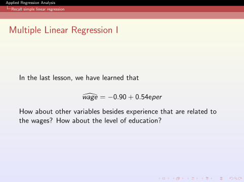
In the last lesson, we have learned that

wage = −0.90 + 0.54eper

How about other variables besides experience that are related tothe wages? How about the level of education?



Multiple Linear Regression II

wage = β0 + β1educ + β2eper + ε

where exper is years of labor market experience and wage is thelevel of education.Multiple regression analysis is also useful for generalizing functionalrelationships between variables. For example, considering therelationship between consumption(cons) and family income(inc):

cons = β0 + β1inc + β2inc2 + ε



Multiple Linear Regression III

After taking x1 = inc and x2 = inc2, it is still a multiple linearregression problem.

Y = β0 + β1X1 + β2X2 + · · ·+ βpXp + ε (3.1)



Multiple Linear Regression IV

According to above equation, each observation can be written as

yi = β0 + β1xi1 + β2xi2 + · · ·+ βpxip + εi



Multiple Linear Regression V

The key assumption of multiple linear regression is :

E (ε|X1, · · · ,Xp) = 0


Parameter Estimation








Parameter Estimation I

The errors can be written as

εi = yi − (β0 + β1xi1 + β2xi2 + · · ·+ βpxip)

The sum of squares of these errors is

S(β0, β1, · · · , βp) =n∑

i=1

ε2i =

n∑i=1

(yi−(β0+β1xi1+β2xi2+· · ·+βpxip))2




In the general case with k independent variables, we seek estimates

β0, β1, · · · , βp

in the equation of

y = β0 + β1x1 + β2x2 + · · ·+ βpxp + ε (3.1)



Parameter Estimation II

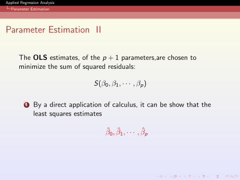
The OLS estimates, of the p + 1 parameters,are chosen tominimize the sum of squared residuals:

S(β0, β1, · · · , βp)

1 By a direct application of calculus, it can be show that theleast squares estimates

β0, β1, · · · , βp



Parameter Estimation III

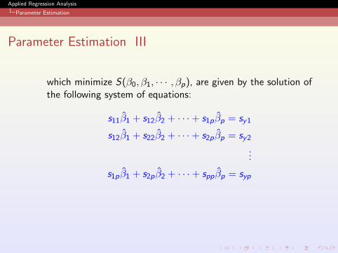
which minimize S(β0, β1, · · · , βp), are given by the solution ofthe following system of equations:

s11β1 + s12β2 + · · ·+ s1pβp = sy1

s12β1 + s22β2 + · · ·+ s2pβp = sy2

...

s1pβ1 + s2pβ2 + · · ·+ sppβp = syp




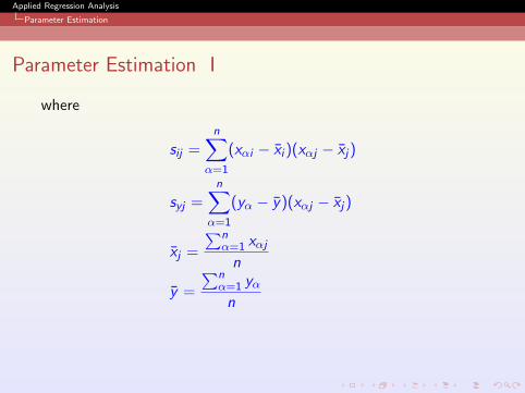
where

sij =n∑

α=1

(xαi − xi )(xαj − xj)

syj =n∑

α=1

(yα − y)(xαj − xj)

xj =

∑nα=1 xαj

n

y =

∑nα=1 yα

n



Parameter Estimation II

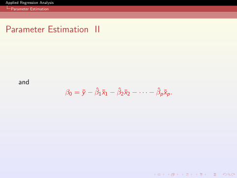
and

β0 = y − β1x1 − β2x2 − · · · − βp xp.



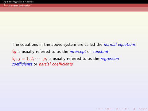
The equations in the above system are called the normal equations.

β0 is usually referred to as the intercept or constant.

βj , j = 1, 2, · · · , p, is usually referred to as the regressioncoefficients or partial coefficients.


Interpretations of Regression Coefficients








Interpretations of Regression Coefficients I

1 β0 is the value of Y when X1 = X2 = · · · = Xp = 0, as in thesimple regression.



Interpretations of Regression Coefficients II

2 βj , j = 1, 2, · · · , p: has several interpretations:

the change in Y corresponding to a unit change in Xj when allother predictor variables are held constant. Magnitude of thechange is not depend on the values at which the otherpredictor variables are fixed.

partial regression coefficient-represents the contribution of Xj

to the response variable Y after it has been adjusted for theother predictor variables.



Interpretations of Regression Coefficients III

3 Ref P57 Explain: Partial regression coefficients



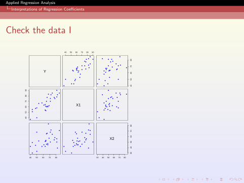
Check the data I

Y

40 50 60 70 80 90

●

●

●

●

●

●

●

●●

●

●

●●

●

●

●

●

● ●

●●

●

●

●

●

●

●

●

●

●

4050

6070

80

●

●

●

●

●

●

●

●●

●

●

●●

●

●

●

●

●●

●●

●

●

●

●

●

●

●

●

●

4050

6070

8090

●

●

●

●

●

●

●

●

●

●

●

●●

●

●

●

●

●

●

●

●

●

●

●

●

●●

●

●

●

X1

●

●

●

●

●

●

●

●

●

●

●

●●

●

●

●

●

●

●

●

●

●

●

●

●

●●

●

●

●

40 50 60 70 80

●

●

●

●

●

●

●

●

●

●

●

●

●

●

●

●

●●

●

●

●

●●

● ●

●

●

●

●

●

●

●

●

●

●

●

●

●

●

●

●

●

●

●

●

●

●●

●

●

●

● ●

● ●

●

●

●

●

●

30 40 50 60 70 80

3040

5060

7080

X2



Check the data II

●

●

●

●

●

●

●

●●

●

●

●

●●

●

●

●

● ●

●●

●

●

●

●

●

●

●

●

●

40 50 60 70 80 90

4050

6070

80

X1

Y



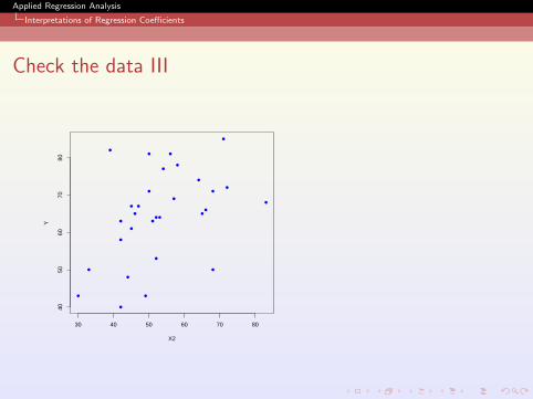
Check the data III

●

●

●

●

●

●

●

●●

●

●

●

●●

●

●

●

●●

●●

●

●

●

●

●

●

●

●

●

30 40 50 60 70 80

4050

6070

80

X2

Y



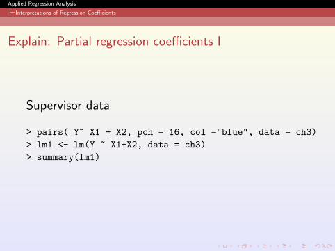
Explain: Partial regression coefficients I

Supervisor data

> pairs( Y~ X1 + X2, pch = 16, col ="blue", data = ch3)> lm1 <- lm(Y ~ X1+X2, data = ch3)> summary(lm1)



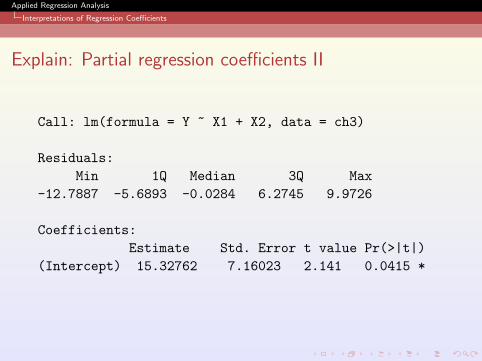
Explain: Partial regression coefficients II

Call: lm(formula = Y ~ X1 + X2, data = ch3)

Residuals:Min 1Q Median 3Q Max

-12.7887 -5.6893 -0.0284 6.2745 9.9726

Coefficients:Estimate Std. Error t value Pr(>|t|)

(Intercept) 15.32762 7.16023 2.141 0.0415 *



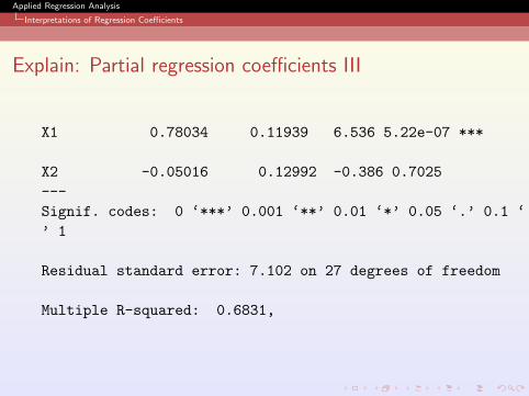
Explain: Partial regression coefficients III

X1 0.78034 0.11939 6.536 5.22e-07 ***

X2 -0.05016 0.12992 -0.386 0.7025---Signif. codes: 0 ‘***’ 0.001 ‘**’ 0.01 ‘*’ 0.05 ‘.’ 0.1 ‘’ 1

Residual standard error: 7.102 on 27 degrees of freedom

Multiple R-squared: 0.6831,



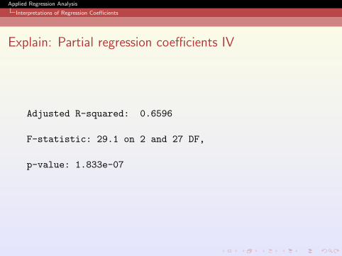
Explain: Partial regression coefficients IV

Adjusted R-squared: 0.6596

F-statistic: 29.1 on 2 and 27 DF,

p-value: 1.833e-07


Properties of the Least Squares Estimators








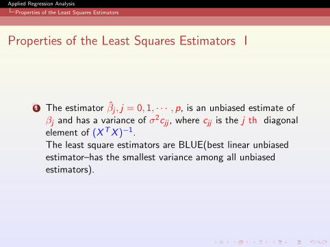
Properties of the Least Squares Estimators I

1 The estimator βj , j = 0, 1, · · · , p, is an unbiased estimate ofβj and has a variance of σ2cjj , where cjj is the j th diagonalelement of (XTX )−1.The least square estimators are BLUE(best linear unbiasedestimator–has the smallest variance among all unbiasedestimators).



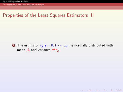
Properties of the Least Squares Estimators II

2 The estimator βj , j = 0, 1, · · · , p , is normally distributed withmean βj and variance σ2cjj .



Properties of the Least Squares Estimators III

3 W = SSE/σ2 has a χ2 distribution with n − p − 1 degree offreedom, and βj ’s and σ2 are distributed independently ofeach other.



Properties of the Least Squares Estimators IV

4 The vector β = (β0, β1, · · · , βp) has a (p + 1)-variate normaldistribution with mean vector β = (β0, β1, · · · , βp) andvariance covariance matrix with elements σ2cij .


Multiple correlation coefficient








Multiple correlation coefficient I

1 The strength of the linear relationship between Y and the setof predictors X1,X2, · · · ,Xp can be assessed through theexamination of the scatter plot of Y versus Y and



Multiple correlation coefficient II

2 the correlation coefficient between Y and Y

Cor(Y , Y ) =

∑(yi − y)(yi − ¯y)√∑(yi − y)2(yi − ¯y)2



Multiple correlation coefficient III

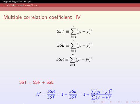
3 Goodness-of-Fit: The coefficient of determination SST: TotalSum of SquaresSSE: Explained Sum of SquaresSSR: Residual Sum of Squares (or Sum of Squared Residuals)



Multiple correlation coefficient IV

SST ≡n∑

i=1

(yi − y)2

SSE ≡n∑

i=1

(yi − y)2

SSR ≡n∑

i=1

(yi − yi )2

SST = SSR + SSE

R2 =SSR

SST= 1− SSE

SST= 1−

∑(yi − yi )

2∑(yi − y)2

4 R2 can be interpreted as the proportion of the total variabilityin the response variable Y that can be accounted for by theset of predictor variables X1,X2, · · · ,Xp.

5 In multiple regression, R =√

R2 is called the multiplecorrelation coefficient

6 A large value of R2 does NOT necessary mean that the modelfits the data well.–Number of predictor variables!

7 adjusted R-squared R2a

R2a = 1− SSE/(n − p − 1)

SST/(n − 1)= 1− n − 1

n − p − 1(1− R2)



Inference for individual regression coefficients I

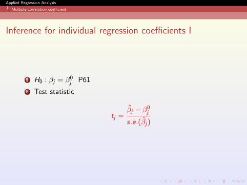
1 H0 : βj = β0j P61

2 Test statistic

tj =βj − β0

j

s.e.(βj)



Inference for individual regression coefficients II

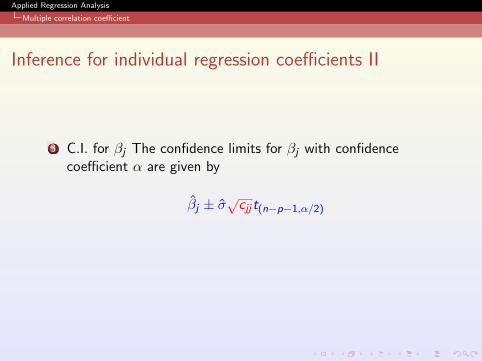
3 C.I. for βj The confidence limits for βj with confidencecoefficient α are given by

βj ± σ√

cjj t(n−p−1,α/2)



Supervisor Performance I

The fitted regression equation is

Y = 10.787+0.613x1−0.073X2+0.320X3+0.081X4+0.038X5−0.217X6

1 How to interpret the outputVariable Coefficient s.e. t-test p-value

Constant 10.787 11.5890 0.93 0.3616X1

X2

X3

X4

X5

X6

n = 30 R2 = 0.73 R2a = 0.60 σ = 7.068 d.f. =23



Supervisor Performance II



Test of Hypothesis in a linear model I

1 All the regression coefficients associated with the predictorvariables are zero.

2 Some of the regression coefficients are zero.

3 Some of the regression coefficients are equal to each other.

4 the regression parameters satisfy certain specified constraints.



Model Compare I

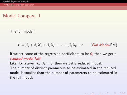
The full model:

Y = β0 + β1X1 + β2X2 + · · ·+ βpXp + ε (Full Model-FM)

If we set some of the regression coefficients to be 0, then we get areduced model-RMLike, for a given k, βk = 0, then we get a reduced model.The number of distinct parameters to be estimated in the reducedmodel is smaller than the number of parameters to be estimated inthe full model.



Model Compare II

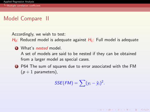
Accordingly, we wish to test:H0: Reduced model is adequate against H1: Full model is adequate

1 What’s nested model.A set of models are said to be nested if they can be obtainedfrom a larger model as special cases.

2 P64 The sum of squares due to error associated with the FM(p + 1 parameters),

SSE (FM) =∑

(yi − yi )2.



Model Compare III

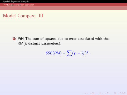
3 P64 The sum of squares due to error associated with theRM(k distinct parameters),

SSE (RM) =∑

(yi − y∗i )2.



Model Compare IV

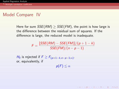
Here for sure SSE (RM) ≥ SSE (FM), the point is how large isthe difference between the residual sum of squares. If thedifference is large, the reduced model is inadequate.

F =[SSE (RM)− SSE (FM)]/(p + 1− k)

SSE (FM)/(n − p − 1)

H0 is rejected if F ≥ F(p+1−k,n−p−1;α).or, equivalently, if

p(F ) ≤ α



Testing all regression coefficients equal to zero I

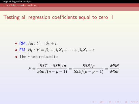
RM: H0 : Y = β0 + ε

FM: H1 : Y = β0 + β1X1 + · · ·+ βpXp + ε

The F-test reduced to

F =[SST − SSE ]/p

SSE/(n − p − 1)=

SSR/p

SSE/(n − p − 1)=

MSR

MSE



Testing a subset of regression coefficients equal to zero I

An important goal in regression analysis is to arrive at adequatedescriptions of observed phenomenon in terms of as fewmeaningful variables as possible.Simplicity of description or the principle of parsimony is one of theimportant guiding principles in regression analysis.



Testing a subset of regression coefficients equal to zero II

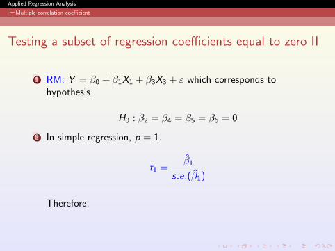
1 RM: Y = β0 + β1X1 + β3X3 + ε which corresponds tohypothesis

H0 : β2 = β4 = β5 = β6 = 0

2 In simple regression, p = 1.

t1 =β1

s.e.(β1)

Therefore,



Testing a subset of regression coefficients equal to zero III

F = t21



Testing the Equality of Regression coefficients I

1

H0 : β1 = β3 (= β′1)|(β2 = β4 = β5 = β6 = 0)

Under H0

2

Y = β′0 + β

′1(X1 + X3) + ε



Estimating and Testing of regression parameters underconstrains I

1

H0 : β1 + β3 = 1|(β2 = β4 = β5 = β6 = 0)

Under H0

2

Y = β0 + β1X1 + (1− β1)X3) + ε



Predictions

1 suppose x0 = (x01, x02, · · · , x0p), the predicted value, y0,corresponding to x0 is given by

y0 = β0 + β1x01 + β2x02 + · · ·+ βpx0p

2 The C.I with confidence coefficient α,

y0 ± t(n−p−1,α/2)s.e.(y0).



Homework

1 P75 3.1∼ 3.5

2 3.15

applied regression analysis - department of …honli/teaching/regression/lecturenotes/lect3.pdf ·...

Documents