statistical quality control for the food industry
TRANSCRIPT


Statistical QualityControl for theFood Industry
Third Edition
Merton R. HubbardConsultant, Hillsborough, California
Kluwer Academic / Plenum PublishersNew York, Boston, Dordrecht, London, Moscow
Library of Congress Cataloging-in-Publication Data
Hubbard, Merton R.Statistical quality control for the food industry/Merton R. Hubbard—3rd ed.
p. cm.Includes bibliographical references and index.ISBN 0-306-47728-91. Food industry and trade—Quality control. I. Title.
TP372.6.H83 2003664'.07—dc21
2003047710
ISBN 0-306-47728-9
Copyright © 2003 by Kluwer Academic/Plenum Publishers, New York233 Spring Street, New York, New York 10013
http: //www. wkap. nl/
1 0 9 8 7 6 5 4 3 2 1
A C.I.P. record for this book is available from the Library of Congress.
All rights reserved
No part of this work may be reproduced, stored in a retrieval system, or transmitted in any formor by any means, electronic, mechanical, photocopying, microfilming, recording, or otherwise,without written permission from the Publisher, with the exception of any material suppliedspecifically for the purpose of being entered and executed on a computer system, for exclusiveuse by the purchaser of the work.
Permissions for books published in Europe: [email protected] for books published in the United States of America: [email protected]
Printed in the United States of America

Preface to theThird Edition
Since the second edition of Statistical Quality Control for the Food Industrywas printed, the statistics involved in the quality control of food has not changed.Sigma is still sigma; the mean remains the mean. There have been some signifi-cant changes however in philosophies, particularly in the areas of quality manage-ment and food quality standards.
The Baldridge National Quality Program has moved another step away fromthe goal of product quality control by emphasizing business excellence as themajor criteria for the Baldridge Award.
As the U.S. imports moved from one foreign country to another, the changingquality of imported manufactured goods in addition to the cost of foreign manu-facture has substantially affected the U.S. national debt.
The major changes in ISO 9000 have resulted in two major concerns: (1) Do thecurrently certified processors have to be recertified? and (2) Since the ISO9000:2000differs in so many areas, does that mean that the quality control procedures of thelast five years were incorrect?
The success of many companies in meeting quality standards using theHACCP principles has been recognized by the FDA. As a direct result, the FDAis increasing the number of food products which must be produced using theHACCP principles. It should be noted that the FDA regulations are concerned withfood safety, rather than food quality, and this is reflected in the new regulations.The need for statistical quality control principles are still required to meet a pro-ducer's needs for other critical food characteristics not included in the HACCPregulations (flavor, color, etc).
Considerable publicity for the six-sigma quality control system has suggestedthat conventional statistical quality control procedures are outmoded. Thismight be true in hardware manufacturing industries where warranties, returns, andrepairs are part of the system, but certainly not in the food industries. However,
there are some parts of the six-sigma approach which might be of value to thefood industry as well.
The Net Content Control regulations have been modified somewhat, but thestatistical approach to compliance remains essentially unchanged.
All of the above changes in the food industry quality control procedures arediscussed in this third edition.
Preface to theSecond Edition
Within the six years since the first edition was published, ISO 9000, HACCP,Expert Systems, six-sigma, proprietary vendor certification programs, sophisti-cated team techniques, downsizing, new electronic and biochemical laboratorymethods, benchmarking, computer-integrated management, and other techniques,standards, and procedures descended upon the quality control managers in thefood industry with the impact of a series of tornados. Everything changed; it wastime to rewrite Statistical Quality Control for the Food Industry.
Or so it seemed. But, as it turns out, everything has not changed. The conceptsof variability, sampling, and probability are still the same. The seven basic toolsof statistical quality control still work. Control charts still supply the informationto control the process—although now the computer is doing most of the calcula-tions and graph construction faster, and in color.
On close examination, even some of the major developments are not really allthat new. For example, ISO 9000 closely resembles Food Processing IndustryQuality System Guidelines published in 1986, and some other quality systems. Thepowerful Hazard Analysis Critical Control Point technique has also been aroundfor some time, and many food companies have been using selected portions of itvoluntarily. Now, however, it has become part of the food laws and has suddenlyreceived widespread publicity.
There have been some real changes, however. The power of the computerhas been applied to several phases of the food industry: Management has foundthat some computer applications can reduce the need for manpower. Other com-puters have been harnessed to processes to receive electrical information, analyzethe input, and instantly send adjustment signals back—thus improvingthe process by reducing variability. Some have been used to instantly provideexpert process advice to the operator. Still others have been used to extract datafrom process computers, and to analyze, calculate, and produce graphs, charts,and reports for product and process improvement studies for immediate use by allinterested departments.

Considering the ability of food processing companies to consistentlymanufacture safe foods with uniform quality over the past 20 or 30 years withoutthese new tools and new systems, one might expect that quality control improve-ments would be marginal. On the other hand, these changes have already providedsubstantial opportunities for process and product improvement. This second editionis intended to update the basic concepts and discuss some of the new ones.
Preface to the First Edition
If an automobile tire leaks, or an electric light switch fails, or we areshort-changed at a department store, or are erroneously billed for phone calls notmade, or a plane departure is delayed due to a mechanical failure—these are fairlyordinary annoyances, which our culture has come to accept as normal occurrences.
Contrast this with a failure of a food product. If foreign matter is found in afood, if the product is discolored or crushed or causes illness or discomfort wheneaten, the consumer reacts with anger, fear, and sometimes mass hysteria. Theoffending product is often returned to the seller, or a disgruntled letter is writtento the manufacturer, or at worst, an expensive law suit may be filed against thecompany. The reaction is almost as severe if the failure is a difficult-to-open pack-age or a leaking container. There is no tolerance for failure of food products.
Dozens of books on quality written for the hardware or service industries dis-cuss failure rates, product reliability, serviceability, maintainability, warranty, andrepairs. Manufacturers in the food industry do not use these measurements sincefood reliability must be 100%, failure rate must be 0%; serviceability, maintain-ability, warranty, and repairs are meaningless.
Consequently, this book on food quality does not concern itself with reliabili-ty and safety. It is assumed that manufacturers in the food industry recognize theintolerance of their customers and the rigid requirement of producing 100% safeand reliable product. Those few food processors who experienced off-flavor, for-eign material, salmonella, botulism, or other serious defects in their productsrarely survive.
What the book does cover are the various techniques which assure the safeproduction of uniform foods. All of the subjects covered are specifically tied tofood industry applications. The chapter on fundamentals of statistics is madepalatable by the use of examples taken directly from companies processing fruits,wine, nuts, and frozen foods. Many other food product examples are used to illus-trate the procedures for generating control charts.
By now, most upper managers are aware that process control is a techniquewhich long ago supplanted the "inspect and sort" concept of quality control. This

book is intended to present upper managers with an understanding of what thetechnique includes. It is also targeted at the quality engineers, managers, and tech-nicians who have been unable to find workable explanations for some of thosequality techniques specifically used by the food industry. A new audience for thissubject includes all of the departments in companies, embracing the concept oftotal quality control. Here is a collection of quality techniques that accounting,procurement, distribution, production, marketing, and purchasing can apply totheir departments. Finally, the book is aimed at students hoping to enter the fieldof food quality control, and technicians who are aspiring to management posi-tions in quality control.
Guidelines for overall quality control systems and suggestions for implement-ing a quality control program are discussed from a generic point of view. All of theother subjects are very specific "how to" discussions. For example, an entire chap-ter is devoted to a step-by-step procedure for controlling the net quantity of pack-aged foods. It explains how to obtain data, interpret government weight regulation,calculate both the legal and economic performance, and set target weights. For themost part, the calculations have been reduced to simple arithmetic.
Where possible, each chapter subject has been designed to stand alone. As anexample, the chapter on process control explains how charts are interpreted andwhat actions should be taken. While reading this chapter on process control, it isnot necessary to thumb through the pages to consult the Appendix tables or thechapter on methods for preparing control charts. Similarly, the design of experi-ments section uses some of the concepts introduced earlier, but does not requirethe reader to review the chapter on fundamentals. The subject of experimentaldesign is complex, but the book reduces it to straightforward explanation andprovides food processing examples, as well as a series of diagrams of the mostuseful designs.
The bibliography contains most of the common texts on statistical processcontrol. In addition, the chapter on test methods provides a list of references,which have food industry applications. The Appendix tables include only thosereferred to in this book.
The author has attempted to avoid theories and generalities in order to makethis book as practical and useful as possible. In the immense field of food pro-cessing, it is remarkable how little specific quality control information has beenavailable. It is hoped that this book will fill that gap.

Acknowledgments
The need for a book of this scope became apparent during the annual presenta-tions of Statistical Process Control Courses for the Food Industry, sponsored bythe University of California, Davis, California. I am primarily grateful to RobertC. Pearl, who spearheaded these quality control courses since the early 1960s, andto Jim Lapsley, his successor, for their continuing support during this book'sdevelopment.
Many University staff and quality professionals have contributed to the prepa-ration and instruction of these courses, and I must give special thanks to thefollowing for permission to include portions of their unpublished notes in varioussections of the book:
Professor Edward Roessler Wendell KerrDr. Alan P Fenech Chip KloosSidney Daniel Ralph LeporiereRonnie L. De La Cruz Jon LibbySeth Goldsmith Donald L. PaulRandy Hamlin Sidney PearceGilbert F. Hilleary Floyd E. WeymouthMary W. Kamm Tom White
Thanks to the Longman Group for permission to reprint Table XXXIII fromthe book Statistical Tables for Biological, Agricultural and Medical Research,6th Edition, 1974, by Fisher and Yates.
Thanks are also due to my wife Elaine for her professional help as my editor,and for her encouragement and patience over the long haul.

v This page has been reformatted by Knovel to provide easier navigation.
Contents
Preface to the Third Edition ............................................. ix
Preface to the Second Edition ......................................... xi
Preface to the First Edition .............................................. xiii
Acknowledgments ........................................................... xv
1. Introduction ............................................................. 1 Variability .............................................................................. 2 Quality Control Programs .................................................... 3 Problems with Tool Selection .............................................. 8 Quality Control Tools ........................................................... 8
2. Food Quality System .............................................. 15 The Formalized Quality System .......................................... 15 Quality System Guidelines .................................................. 16 Malcolm Baldridge National Quality Award ......................... 27 Total Quality Management .................................................. 28 Team Quality Systems ........................................................ 30 Computer Network Quality Systems ................................... 30 Summary .............................................................................. 30
3. Control Charts ......................................................... 49 The Importance of Charting ................................................. 49

vi Contents
This page has been reformatted by Knovel to provide easier navigation.
Procedure for Constructing X-Bar and R Charts ................. 53 Procedures for Constructing Attribute Charts ..................... 57
4. Fundamentals .......................................................... 71 Analysis of Data ................................................................... 71 Probability ............................................................................ 76 Binomial Distribution ............................................................ 78 The Normal Distribution ....................................................... 82 Distribution of Sample Means ............................................. 84 Normal Approximation to the Binomial Distribution ............ 90 t-Distribution ......................................................................... 92 Confidence Limits for the Population Mean ........................ 93 Statistical Hypotheses – Testing Hypotheses ..................... 95 Distribution of the Difference between Means .................... 100 Paired Observations ............................................................ 103 F-Distribution ........................................................................ 104 Analysis of Variance ............................................................ 105 Two Criteria of Classification ............................................... 111
5. Sampling .................................................................. 115 Sampling Plans .................................................................... 115 Why Sample? ...................................................................... 116 Samples from Different Distributions ................................... 117 Sample Size ......................................................................... 118 How to Take Samples ......................................................... 123 Types of Samples ................................................................ 128 Sampling Plans .................................................................... 131 Types of Inspection .............................................................. 131 Classes of Defects ............................................................... 132 Sampling Risks .................................................................... 135 Selection of Population to be Sampled ............................... 136

Contents vii
This page has been reformatted by Knovel to provide easier navigation.
Selection of Sample Frequency and Location .................... 137 Hazard Analysis Critical Control Point ................................. 138 Attribute Sampling Plans ..................................................... 149
6. Test Methods ........................................................... 151 General Analysis .................................................................. 153 Special Instrumentation ....................................................... 153 Microbiology ......................................................................... 153 Sensory ................................................................................ 153
7. Product Specifications ........................................... 157
8. Process Capability .................................................. 163 Capability Index ................................................................... 170 Benchmarking ...................................................................... 173
9. Process Control ...................................................... 177 Chart Patterns ...................................................................... 179 Using the Control Chart as a Quality Management
Tool ........................................................................... 184
10. Sensory Testing ...................................................... 187 The Senses .......................................................................... 188 Sensory Testing Methods .................................................... 189 Types of Panels ................................................................... 194 Selection and Training ......................................................... 197
11. Net Content Control ................................................ 201 Evaluation of Net Content Performance .............................. 205 Interpreting Net Content Control ......................................... 205 Procedures for Setting Fill Targets ...................................... 213
viii Contents
This page has been reformatted by Knovel to provide easier navigation.
12. Design of Experiments ........................................... 219 Introduction .......................................................................... 219 Elimination of Extraneous Variables ................................... 222 Handling many Factors Simultaneously .............................. 226 Full Factorial Designs .......................................................... 227 Fractional Factorial Designs ................................................ 232 Response Surface Designs ................................................. 236 Mixture Designs ................................................................... 239 Experimental Design Analysis by Control Chart ................. 248
13. Vendor Quality Assurance ..................................... 253 Vendor-Vendee Relations ................................................... 255 Specifications for Raw Materials, Ingredients, Supplies ..... 257 Quality Assurance of Purchased Goods ............................. 259 Selecting and Nurturing a Supplier ...................................... 263 Packaging Supplier Quality Assurance ............................... 266 Supplier Certification Programs ........................................... 271
14. Implementing a Quality Control Program ............. 275 Management Commitment .................................................. 275 Getting Started ..................................................................... 276 An In-House Program .......................................................... 277 Team Quality Systems ........................................................ 279 Stepwise Procedures for Team Problem Solving ............... 282 Programs without Management Support ............................ 284 Training Quality Control Technicians .................................. 287 Summary .............................................................................. 288
15. The Computer and Process Control ...................... 289 Computer Integrated Management ..................................... 289 Artificial Intelligence and Expert Systems ........................... 291
Contents ix
This page has been reformatted by Knovel to provide easier navigation.
Computer-Controlled Processing ........................................ 294 Summary .............................................................................. 307
16. Six-Sigma ................................................................. 309 Summary .............................................................................. 313
Appendix ........................................................................ 315
References ..................................................................... 335
Index ............................................................................... 339
1 Introduction
In 2002, the United States balance of trade with East Asia was negative$171,593,000. The prices were not necessarily lower than for merchandise pro-duced in the United States, but the quality level and uniformity were excellent—a far cry from the shoddy reputation the Orient suffered throughout the first halfof the 20th century. This has raised fears that the Orient would ultimately takeover the production of all of our products, and that the United States has alreadyturned into a service-industry nation. Statisticians have been known to generateanalyses that are mathematically correct, but which occasionally are open toquestion if the data are presented out of context. The 171 billion dollars may fallinto that category. There is no question that the 171 billion dollars represents asizeable quantity of goods; but the yearly US. Gross National Product (GNP) inthe early 200Os was 10 trillion dollars. This means that imports from East Asiaaccounted for only 1.7% of our GNP. Less than 2% does not seem to be a dan-gerously high level—certainly not high enough to suggest that we are in dangerof having all of our products manufactured elsewhere.
Government statisticians have replaced GNP with Gross Domestic Product(GDP), but there is only a small difference between these figures. Perhaps the1.7% figure might be overly pessimistic, because trade imbalances have built-incorrecting devices. For example, during periods when domestic consumptionslows, imports will slow as well. U.S. exports during the end of the century wereactually growing at a 25% annual rate, and trade deficits with foreign countrieshad peaked. This improvement was masked by the fluctuating value of thedollar against foreign currencies. (Merrill Lynch Global Investment Strategy,21 March 1995; also the Japan Business Information Center; Keizai KohoCenter.)
The quality control and the quality level in the United States are not necessarilyinferior, as implied by the cold numbers. Perhaps the impression that our manu-facturing industry is about to be taken over by the Orient is due to their selectionof some highly visible consumer products. They have done an excellent job of itin photography, optics, electronics and the auto industry. But even in these areas,

the United States still maintains a significant number of profitable operationswith notable market share.
Food production and processing in the United States is an area of outstandingquality, unmatched by the Orient. The most obvious example of food quality con-trol is the safety of foods in the United States. There are 290 million people in thiscountry who eat a total of about 870 million meals a day, or 318 billion mealsannually. A benchmark study made by the Center for Disease Control analyzedthe numbers and causes for food outbreaks across the country for an entire year.They found 460 reported outbreaks of food poisoning, in which an outbreak wasdefined as two or more people becoming ill from the same food eaten at the sametime. The 460 figure represents the number of people who were reported byPublic Health Departments, doctors, and hospitals to have become ill from foodsduring the year, but does not include those who became ill and who went to theirown physician for treatment or waited without assistance until they recovered.Of course, such data is unavailable. Working only with the proven data, the 460figure, expressed as percent product failure, indicates
(460 X 100)7318,000,000,000 = 0.000000147%
It is difficult to find another country which has achieved that kind of record forany product in any industry.
If the record for food quality is so superb, why this book? Because the need toimprove quality control is unending. The safety appears adequate, but there arealways improvements possible in net weight control, product color, flavor, keep-ing qualities, production cost, absence of defects, productivity, etc. There still islittle factual quality information provided at the graduate level of businessschools, and much of the information available to the management of food pro-cessing companies is supplied by the professionals in quality control who arelikely to read this book. Perhaps management may find the time to read it as well.
VARIABILITY
We live in a world of variability. The person who first used the expression"like two peas in a pod" was not looking very carefully. There are no two peopleexactly alike—even so-called twins. Astronomers tell us that in this vast universe,there are no two planets alike. Two man-made products which are "within speci-fications" may seem to be the same, but on closer inspection, we find that theyare not identical.
It is generally known that perfection is not possible. You know it, your friendsknow it, children know it; but the Chief Operating Officer of many companiesdoes not admit to it. He says that there is no reason why all products in a properlymaintained production line—with adequately trained and motivated workers,the right raw materials, expert supervisors, and quality control employees whoknow what they are doing—cannot be perfectly uniform, with no defects, andwith no variation. While we must accept the fact that variability does exist, there
are methods to control it within bounds which will satisfy even the ChiefOperating Officer. You will find that:
• Statistical tools are available• Processes can be controlled• Line people are not necessarily responsible for poor quality• Management, and only management can improve quality
QUALITY CONTROL PROGRAMS
The Shewhart control-chart technique was developed in 1924, and has been in usecontinuously since then. Perhaps the only fundamental change in the Shewhartchart was the simplification evolved by mathematical statisticians by which con-trol charts could be simply determined using the range of observations, ratherthan the more time-consuming calculations for standard deviations for each sub-group. Evaluation of the statistical approach of Shewhart was published in 1939by WE. Deming, who later (1944) defined "constant-cause systems, stability, anddistribution" in simple terms to show how a control chart determined when aprocess was in statistical control. After over 50 years, these principles are stillvalid, and are the basis for most of the successful quality control programs in usetoday.
One of the philosophies attributed to Dr. Deming is that judgment and theeyeball are most always wrong. X-bar, R and/? charts are the only evidence that aprocess is in control. Failure to use statistical methods to discover which type ofcause (common or system cause; and special or assignable cause) is responsiblefor a production problem generally leads to chaos; whereas statistical methods,properly used, direct the efforts of all concerned toward productivity and quality.
Dr. Deming has stated that 85% of the causes of quality problems are faults ofthe system (common causes) which will remain with the system until they arereduced by management. Only 15% of the causes are special or assignable causesspecific to an individual machine or worker, and are readily detectable fromstatistical signals. Confusion between common and assignable causes leads tofrustration at all levels, and results in greater variability and higher costs—theexact opposite of what is needed. Without the use of statistical techniques, thenatural reaction to an accident, a high reject rate, or production stoppage is toblame the operators.
The worker is powerless to act on a common cause. The worker has no authorityto sharpen the definition and tests that determine what constitutes acceptablequality. He cannot do much about test equipment or machines which are out oforder. He cannot change the policy or specifications for procurement of incomingmaterials, nor is he responsible for design of the product.
Several quality control leaders have each developed a formalized programconsisting of several steps. It is difficult to look at a summary of these steps todetermine which system is best for a given company, since the programs must betailored to each particular situation. Note how even these recognized authorities
disagree on certain measures. A summary of the steps suggested by these qualitycontrol authorities follows. They are not complete descriptions, but serve todifferentiate the emphasis of these programs.
J.M. Juran
1. Establish quality policies, guides to managerial action.2. Establish quality goals.3. Design quality plans to reach these goals.4. Assign responsibility for implementing the plans.5. Provide the necessary resources.6. Review progress against goal.7. Evaluate manager performance against quality goal.
W.E. Deming (Quality Magazine Anniversary Issue 1987)
1. Create constancy of purpose toward improvement of product and services.2. Adopt the new philosophy: we are in a new economic age.3. Cease dependence on mass inspection as a way to achieve quality.4. End the practice of awarding business on the basis of price tag.5. Constantly and forever improve the system of production and service; the
system includes the people.6. Institute training on the job.7. Provide leadership to help people and machines do a better job.8. Drive out fear.9. Break down barriers between departments.
10. Eliminate slogans and targets for zero defects and new productivity levels.11. Eliminate work standards and management by objectives.12. Remove barriers that rob people of their right to pride of workmanship.13. Institute a vigorous program of education and self-improvement.14. Put everybody in the company to work to accomplish the transformation.
Armand V. Fiegenbaum
1. Agree on business decision at the boardroom level to make quality lead-ership a strategic company goal and back it up with the necessary budgets,systems, and actions. Each key manager must personally assess perform-ance, carry out corrective measures, and systematically maintainimprovements.
2. Create a systemic structure of quality management and technology. Thismakes quality leadership policies effective and integrates agreed-uponquality disciplines throughout the organization.
3. Establish the continuing quality habit. Today's programs seek continuallyimproving quality levels.

Tom Peters
1. Abiding management commitment.2. Wholesale empowerment of people.3. Involvement of all functions—and allies of the firm.4. Encompassing systems.5. Attention to customer perceptions more than technical specifications.
RB. Crosby (Quality is Free by RB. Crosby)
1. Management commitment.2. Quality improvement team.3. Quality measurement.4. Cost of quality evaluation.5. Quality awareness.6. Corrective action.7. Establish an Ad Hoc committee for the Zero Defects Program.8. Supervisor training.9. Zero defects day.
10. Goal setting.11. Error cause removal.12. Recognition.13. Quality councils.14. Do it all over again.
M.R. Hubbard (N. CaI. Institute of Food TechnologistsOctober 1987)
1. Select an area within the company in need of assistance, using Pareto orpolitical procedures.
2. Using statistical techniques, calculate process capability and determinecontrol limits.
3. Establish sampling locations, frequency, size, and methods of testingand reporting. Study process outliers and determine assignable causes ofvariation at each process step.
4. Correct assignable causes by modifying the process, and calculateimproved process capability. Report to management dollars saved,improved productivity, reduced scrap, rework, spoilage, product giveaway,overtime, etc.
5. Repeat steps 3 and 4 until no further improvements are apparent.6. Design experiments to modify the process to further improve productivity,
and follow by returning to step 2, using the most promising test results.7. Move on to another area of the company (another line, another function,
another department) until the entire company is actively pursuing qualityprograms.

8. Where possible, install quality attribute acceptance sampling plans as asafeguard for quality in the process and in the finished product. Expandthis into a company-wide audit system.
Total Quality Management Practices (General AccountingOffice 1991)
1. Customer-defined quality.2. Senior management quality leadership.3. Employee involvement and empowerment.4. Employee training in quality awareness and quality skills.5. Open corporate culture.6. Fact-based quality decision-making.7. Partnership with suppliers.
Hazard Analysis Critical Control Point (Department of Healthand Human Services—FDA, 1994-2002)
1. Identify food safety hazards.2. Identify critical control points where hazards are likely to occur.3. Identify critical limits for each hazard.4. Establish monitoring procedure.5. Establish corrective actions.6. Establish effective record keeping procedures.7. Establish verifying audit procedures.
Computer Integrated Management (approximately 1987)
Computer integrated management (CIM) is a system designed to control allphases of a food process by the use of computers. The goal is to utilize computerpower in product design, engineering, purchasing, raw material control, produc-tion scheduling, maintenance, manufacturing, quality control, inventory control,warehousing and distribution, cost accounting, and finance. By integrating thedatabases and commands of the individual computer systems throughout all ofthese stages, it should be possible to improve the efficiency of production plan-ning and control, decrease costs of each operation, and improve both process con-trol and product quality. The goal is to optimize the entire system through the useof computerized information sharing.
ISO 9000 Standards (International Organization forStandardization revised 2000)
1. ISO 9000. Quality Management and Quality Assurance Standards—Guidelines for Selection and Use.

The 2002 emphasis shifted further from product quality control toward businessperformance excellence. The Examination categories for 2002 were:
• Leadership• Strategic planning• Customer and market focus• Information and analysis• Human resource focus• Process management• Business results.
Although these business goals are admirable, they have failed to emphasize thegoal of quality control.
Six-Sigma (Motorola 1979) (see Chapter 16)
• Recognize• Define• Measure• Analyze• Improve• Control• Standardize• Integrate.
2. ISO 9001. Quality Systems—Model for Quality Assurance in Design/Development, Production, Installation, and Servicing.
3. ISO 9004. Quality Management and Quality System Elements—Guidelines.
Malcolm Baldridge National Quality Award (U.S. Department ofCommerce 1987, and revised annually)
The seven categories on which these quality awards are based have been revisedover the years. Three years have been selected at random as examples.
1990 Examination categories
1. Leadership2. Information and analysis3. Strategic quality planning4. Human resources utilization
5. Quality assurance of productsand services
6. Quality results7. Customer satisfaction
1 995 Examination categories
LeadershipInformation and analysisStrategic planningHuman resource developmentand managementProcess management
Business resultsCustomer focus and satisfaction

The Six-Sigma process is often called the DMAIC system, referring to thesteps 2-6 above. The system is explained in detail in Chapter 16.
Other Quality Programs
Since the 1980s, several additional techniques have been offered with the goal ofimproving quality control programs. For the most part, they are business processtools rather than statistical quality control techniques, but have often had favorableeffects on both productivity and product quality. Some of the many examples:Total Quality Management, Teams, Reengineering, Benchmarking, Empowerment,Continuous Improvement, Quality Function Deployment, Computer Applications,Six-Sigma, Computer Controlled Processes, Computer Analyses of Data,Computerized SPC, Real Time Manufacturing, Expert Systems, etc.
PROBLEMS WITH TOOL SELECTION
The difficulty in selecting the correct statistical tools for problem solving mightbe explained using the analogy of selecting the correct tools for a painting project.Assume that we wish to paint a rod. We are faced with the following choices:
5 finishes: flat, satin flat, satin, semigloss, gloss3 solubilities: oils, water, organic solvents5 types: lacquers, enamels, stains, primers, fillers4 spreaders: air and pressure spray, roll, brush, gel brush
Although all of these possibilities are not necessarily combinable, there is apossibility of at least
5 X 3 X 5 X 4 = 3 OO combinations of kinds of paints and applicators
This does not include all paint types, or the myriad of shades available. Nor doesit consider the formulations for floor, ceiling, deck, wall, furniture, concrete,metal, glass, antifouling, etc. Nor does it include subclasses of metals: iron, gal-vanized, copper, aluminum, etc. Knowing which tools are available may not solveour painting problem. Any paint will cover wood, concrete, or some metals, butwill it peel, blister, fade, discolor, weather, corrode, flake, or stain? Will it leavebrush marks, or a slippery surface? Is it toxic? Does it have an unpleasant odor?Will it resist a second coat? In short, knowing which tools are available is neces-sary; and knowing the proper use of these tools is absolutely imperative.
QUALITY CONTROL TOOLS
The following is a list of the more common statistical tools used in qualitycontrol applications. These will be covered in greater detail later. These tools have
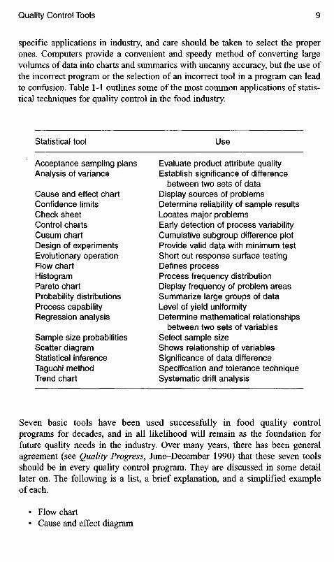
Statistical tool
Acceptance sampling plansAnalysis of variance
Cause and effect chartConfidence limitsCheck sheetControl chartsCusum chartDesign of experimentsEvolutionary operationFlow chartHistogramPareto chartProbability distributionsProcess capabilityRegression analysis
Sample size probabilitiesScatter diagramStatistical inferenceTaguchi methodTrend chart
Use
Evaluate product attribute qualityEstablish significance of difference
between two sets of dataDisplay sources of problemsDetermine reliability of sample resultsLocates major problemsEarly detection of process variabilityCumulative subgroup difference plotProvide valid data with minimum testShort cut response surface testingDefines processProcess frequency distributionDisplay frequency of problem areasSummarize large groups of dataLevel of yield uniformityDetermine mathematical relationships
between two sets of variablesSelect sample sizeShows relationship of variablesSignificance of data differenceSpecification and tolerance techniqueSystematic drift analysis
Seven basic tools have been used successfully in food quality controlprograms for decades, and in all likelihood will remain as the foundation forfuture quality needs in the industry. Over many years, there has been generalagreement (see Quality Progress, June-December 1990) that these seven toolsshould be in every quality control program. They are discussed in some detaillater on. The following is a list, a brief explanation, and a simplified exampleof each.
• Flow chart• Cause and effect diagram
specific applications in industry, and care should be taken to select the properones. Computers provide a convenient and speedy method of converting largevolumes of data into charts and summaries with uncanny accuracy, but the use ofthe incorrect program or the selection of an incorrect tool in a program can leadto confusion. Table 1-1 outlines some of the most common applications of statis-tical techniques for quality control in the food industry.

• Control chart (variable and attribute)• Histogram• Check sheet• Pareto chart• Scatter diagram.
Table 1 -1. Use of SQC Techniques in the Food Industry
Statistical techniques
A. Experimental design: Factorial, ANOVA, regression, EVOP, TaguchiB. Control charts: X-bar, R, p, np, cC. Acceptance sampling: Attributes MIL STD 105E, variables MIL STD 414D. Diagrams: Pareto, cause and effectE. Special sampling: Skiplot, cusum, scatter diagram, flow chart, histogram,
check sheetF. Special charts: Sequential, trend analysis. Consumer complaints
Applications
Product designSpecifications: Product, ingredient, packagingSensory evaluationFunction, shelf life
Process designProcess specification, process capability
VendorSelection, qualification, control
Incoming qualityMaterials, supplies
Process specification conformanceSort, clarify, wash, heat, filter, cool, mill, otherPackage integrity, code, fill, appearanceMicrobiology
Product specification conformanceSensory — color, flavor, odorStructure, function
Storage and distribution
Consumer complaints
AuditLaboratory controlProcess, product, field performance
Product, process improvement
Use technique
A
A1B
B,C
B,C
B,C,E,F
B,C
B,C
B,D
A,B,C
A,D,F
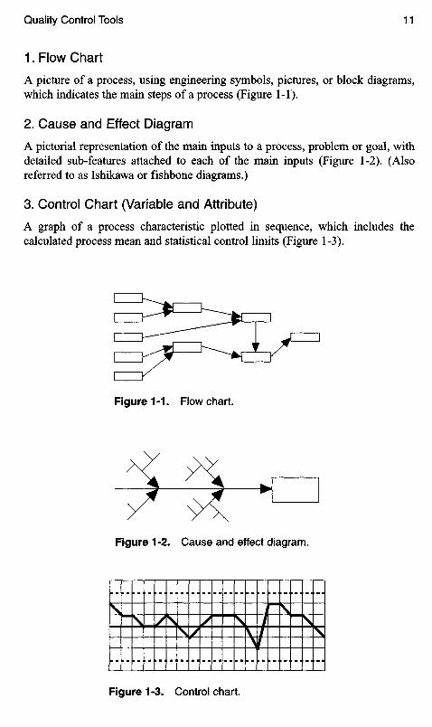
1. Flow Chart
A picture of a process, using engineering symbols, pictures, or block diagrams,which indicates the main steps of a process (Figure 1-1).
2. Cause and Effect Diagram
A pictorial representation of the main inputs to a process, problem or goal, withdetailed sub-features attached to each of the main inputs (Figure 1-2). (Alsoreferred to as Ishikawa or fishbone diagrams.)
3. Control Chart (Variable and Attribute)
A graph of a process characteristic plotted in sequence, which includes thecalculated process mean and statistical control limits (Figure 1-3).
Figure 1-1. Flowchart.
Figure 1-2. Cause and effect diagram.
Figure 1-3. Control chart.

Figure 1-4. Histogram.
Figure 1-5. Check sheet.
Figure 1-6. Pareto chart.
Figure 1-7. Scatter diagram.

4. Histogram
A diagram of the frequency distribution of a set of data observed in a process(Figure 1-4). The data are not plotted in sequence, but are placed in the appropriatecells (or intervals) to construct a bar chart.
5. Check Sheet
Generally in the form of a data sheet, used to display how often specific problemsoccur (Figure 1-5).
6. Pareto Charts
A bar chart illustrating causes of defects, arranged in decreasing order.Superimposed is a line chart indicating the cumulative percentages of thesedefects (Figure 1-6).
7. Scatter Diagrams
A collection of sets of data which attempt to relate a potential cause (X-axis) withan effect (Y-axis) (Figure 1-7). Data are collected in pairs at random.

2 Food Quality System
THE FORMALIZED QUALITY SYSTEM
As a company grows, the need for formal departmental operating procedures andreports generally produces a large volume of standard manuals. The QualityDepartment in a food manufacturing company may be the last one to assemble awritten system. There are perhaps more excuses than reasons for this:
• The products change from year to year, and someone would have to beretained on the Quality Department payroll just to keep up with thepaperwork. (Unrealistic!)
• The food industry is regulated by federal agencies (Food and Drug,Commerce, Department of Agriculture, and others) and by state and localagencies (Weights and Measures, Public Health, and others). Therefore,there is no need to further formalize quality procedures. (Untrue!)
• A food processing company could not remain in business unless its qualitysystems were adequate. It might be risky to change the existing system.(Head in the sand!)
• It is necessary to remain flexible in the food business so that the companycan take advantage of new developments quickly. A formalized system tendsto slow things down. (Absence of a system may bring things to a standstill!)
These excuses might be applied equally to other departments within a foodcompany (accounting, personnel or distribution), but companies generally haverigorous formalized procedures for these departments. The Quality Departmenthas frequently been overlooked in this respect, partly because it is a relatively newdiscipline. The "Food Processing Industry Quality System Guidelines" wasprepared for the American Society for Quality Control in 1986. Prior to that time,the Society, the professional organization dedicated to promotion of qualitycontrol in industry, had no recommendations specifically for the food industry.
15

Perhaps a more common reason for the lack of system emphasis of quality isthat the techniques of statistical quality control are not well understood by uppermanagement. Until the 1980s, few colleges or universities offered degrees instatistical quality control. In fact, few even offered classes in this subject. Asa direct result, quality control was far too often mistakenly considered to beconcerned with inspection, sorting, sanitation management, and monitoring theretorting process for low acid canned foods.
Quality control in the food industry, under these conditions, quite naturallywas regarded as a cost center which contributed to overhead, rather than as apotential profit center which contributed to savings. From a series of successes athome and abroad in quality control—quality improvement, process improvement,productivity improvement, reduction in cost of scrap, rework, and productgiveaway—the reputation of properly organized and operated quality controldepartments has gradually changed from a "cost generator" to a "profit center."
A quality system which starts at the product concept and development stagehas the greatest opportunity to reduce new product costs. The cost to remedydesign failures is minimized when these shortcomings are detected at theconcept or prototype stages of development. The cost to remedy failures risesexponentially at the later stages (pilot plant, production run, market distribution).A documented system can assure that geographically separated divisions of acompany know how to produce uniform product quality, and are capable ofcommunicating process improvement information between plants. Such a systemprovides an effective tool for training new employees both within and outside ofthe quality department. Perhaps most important, a documented quality system canbe created to emphasize continuously the twin goals of attainment of uniformquality and profit improvement.
QUALITY SYSTEM GUIDELINES
Chapter 1 outlined nearly a dozen approaches to developing a quality system.A more detailed discussion of some of the more recent system guidelines follows.It should be emphasized that the seven basic tools of quality should be includedin each of these systems.
Six-sigma (see Chapter 8) is based on counting defects, and using this data torate quality control. Efforts to reduce the number of defects are centered aroundinputs from all levels of employment within the company. Management andemployees all train in the statistics involved, the techniques of production inspec-tion and product improvement. It is most effective in hardware industries wheredefects can be remachined or sorted and scrapped. For the most part, this indus-try's standards are self-imposed by the manufacturers or their customers. Becauseof legal standards (and complete unwillingness by consumers to accept any fooddefects) the six-sigma method has little application to the food industry.
HACCP (see Chapter 5) is centered on food production industries, and is basedon defect prevention. Critical path diagrams are generally clear flow diagrams

which can be understood by production personnel, thus contributing to theireffectiveness. Unlike most hardware industries where some defective product isconsidered normal (though undesirable), in the food industry critical defects arenot acceptable, and in many areas not permitted by law.
ISO 9000:2000 (see below) is an excellent tool to enforce control of quality. Itis effective in the hardware industries. Food industries may be required to adhereto this standard in order to export their products to many countries which demandISO certification.
TQM, PDAC, and many other pseudonyms are based on detailed standards(often legislated) which are achieved by the use of statistical quality controls. Theprinciples may not be understood at all levels of employees, but these programscan be highly effective for preventing defects, improving quality and loweringprocess costs.
Food Processing Industry Quality System Guidelines
The generic guidelines for quality systems developed by the American NationalStandards Institute (ANSI Z 1.15) provides an excellent basis for establishingeffective quality control systems, but is geared more toward hardware manufac-ture than food processing. A committee of food quality experts, chaired bySydney Pearce, restructured this standard for use by the food processing industry,and published the guidelines in 1986. This document covers the following:
1. Administration includes quality policy, objectives, quality system, planningquality manual, responsibility, reporting, quality cost management,and quality system audits. Each of these subjects is covered in detail. Forexample, quality system provides for individual policies, procedures, stan-dards, instructions, etc. covering: ingredients, packaging, processing, fin-ished product, distribution, storage practices, vendor/contract processorsrelations, environmental standards, sanitation, housekeeping, pestmanagement/control, shelf life, design assurance, recall, quality costs, usercontacts, complaint handling and analysis, corrective action, motivationaland training programs and others.
2. Design assurance and design change control contains 12 subsections,such as concept definition, design review, market readiness review.
3. Control of purchased materials—an excellent summary of suppliercertification requirements, such as specifications, system requirements,facility inspection, assistance to suppliers.
4. Production quality control contains 24 detailed requirements under thefollowing subheadings:• Planning and controlling the process• Finished product inspection• Handling, storage, shipping• Product and container marking• Quality information.

5. User contact and field performance includes product objective, advertising,marketing, acceptance surveys, complaints and analysis.
6. Corrective action covers detection, documentation, incorporating change,product recall, and non-conforming disposition.
7. Employee relations—selection, motivation, and training.
Good Manufacturing Practice (GMP)
Although not one of the statistical tools of quality control, GMPs belong in everyfood quality control system. The Code of Federal Regulations (CFR 21 Part 110,GMP) provides excellent definitions and criteria which determine if the producthas been manufactured under conditions which make it unfit for food; or if theproduct has been processed under insanitary conditions resulting in contamina-tion with filth; or is otherwise rendered injurious to health. It contains detailedrequirements for avoiding these possibilities in the following general areas:
Personnel—Disease control, cleanliness, education and training, and supervision.Plant and grounds—Proper equipment storage, maintenance of surrounding
property, effective systems for waste disposal, space for equipment place-ment and storage of materials, separation of operations likely to causecontamination, sanitation precautions for outside fermentation vessels,building construction to permit adequate cleaning, adequate lighting,ventilation and screening.
Sanitary operations—Building and Fixtures: maintenance, cleaning andsanitizing to prevent contamination. Special precautions for toxic sanitizingagents. Pest control. Food contact surfaces: sanitation procedures.
Sanitary facilities and controls—Water supply, plumbing, sewage disposal,toilet facilities, handwashing facilities, rubbish and offal disposal.
The Code then follows with specific GMP regulations for equipment and forprocess controls.
Equipment and utensils—Design, materials and workmanship shall be cleanable,protected against contamination, and shall be nontoxic, seamless, and prop-erly maintained. (Some specific types of equipment are referred to: holding,conveying, freezing, instrumentation, controls, and compressed gases.)
Processes and controls—Adequate sanitation in receiving inspection, trans-porting, segregating, manufacturing, packaging, and storing. Appropriatequality control operations to insure that food is suitable for humanconsumption and that packaging materials are safe and suitable. Assignedresponsibility for sanitation. Chemical, microbial and extraneous materialtesting. Rejection of adulterated or contaminated material.• Raw materials—Shall be inspected for suitability for processing into
food. Stored to minimize deterioration. Wash and conveying water to beof adequate sanitary quality. Containers shall be inspected for possiblecontamination or deterioration of food. Microorganism presence shallnot be at a level which might produce food poisoning, and shall be

pasteurized during manufacturing to maintain a safe level. Levels oftoxins (such as aflotoxin), or presence of pest contamination or extra-neous material to be in compliance with FDA regulations, guidelines oraction levels. Storage of raw materials, ingredients or rework shall beprotected against contamination, and held at temperature and humiditywhich will prevent adulteration. Frozen raw materials shall be thawedonly as required prior to use and protected from adulteration.
• Manufacturing operations—Equipment, utensils and finished foodcontainers to be sanitized as necessary. Manufacturing, packaging andstorage to be controlled for minimum microorganism growth, or con-tamination. (A number of specific suggestions for physical factors to becontrolled: time, temperature, humidity, water activity, pH, pressure,flow rate. Controls for manufacturing operations are also suggested:freezing, dehydration, heat processing, acidification, and refrigeration.)Growth of undesirable organisms shall be prevented by refrigeration,freezing, pH, sterilizing, irradiating, water activity control. Constructionand use of equipment used to hold, convey or store raw materials, ingre-dients work in process, rework, food or refuse shall protect against con-tamination. Protection against inclusion of metals or other extraneousmaterial shall be effective. Adulterated food, ingredients or raw materi-als shall be segregated and, if reconditioned, shall be proven to be effec-tively free from adulteration. Mechanical manufacturing steps such aswashing, peeling, trimming, cutting, sorting, inspecting, cooling, shred-ding, extruding, drying, whipping, defatting, and forming shall be per-formed without contamination. Instructions are offered for blanching,with particular emphasis on thermophilic bacteria control.
Preparation of batters, breading, sauces, gravies, dressings and simi-lar preparations shall be prepared without contamination by effectivemeans such as: contaminant-free ingredients, adequate heat processes,use of time and temperature controls, physical protection of compo-nents from contaminants which might be drawn into them during cool-ing, filling, assembling and packaging.
Compliance may be accomplished by a quality control operation inwhich critical control points are identified and controlled during opera-tion; all food contact surfaces are cleaned and sanitized; all materialsused are safe and suitable; physical protection from contamination, par-ticularly airborne, is provided; and sanitary handling procedures are used.
Similar requirements are listed for dry mixes, nuts, intermediatemoisture food, dehydrated foods, acidified foods, and ice-added foods.Lastly, the regulation forbids manufacturing human and non-humanfood grade animal feed (or inedible products) in the same areas, unlessthere is no reasonable possibility for contamination.
• Warehousing and distribution—Storage and transportation of finishedfoods shall be protected against physical, chemical and microbial con-tamination, as well as deterioration of the food and the container.

Food processing companies with sufficient staff might consider incorporating theGMP regulation in the quality control manual, and conducting routine audits toassure conformance. Consulting firms are available to perform periodic GMPinspections for smaller organizations. In either case, a file of satisfactory auditscould prove invaluable in the event of suspected product failure resulting inlitigation.
It should be noted that the FDA regulations for Good Manufacturing Practiceis modified from time to time, and it is necessary to periodically review qualitycontrol procedures to insure compliance.
ISO Standards (International Organization forStandardization, Revised 2000)
The International Organization for Standardization in Geneva, Switzerland, beganto develop a series of standards to describe an ideal, generic quality system in thelate 1970s. Based on the British quality standard, the initial intent was to clarifycontracts between suppliers and their customers. It became apparent after a fewyears, that companies which were registered for compliance with these standardswould not require most supplier audits, since customers could be assured ofproduct which would meet their specifications. Some countries have expandedthis concept to require that imported goods must be produced under ISO standards.Although the ISO requires that all standards be reviewed and updated everyfive years, it was expected that changes would be gradual. The 1994 changes, forexample, included relatively minor format and wording, a greater emphasis ondocumented procedures (including the quality manual), a few small additions tomanagement responsibility and staffing, addition of a quality planning document,and a few definitions such as verification and validation.
There are three Standards in the revised ISO 9000 series: 9000, 9001, and9004. The 1994 standards 9002 and 9003 have been discontinued, and theircoverage has been consolidated into the 9001 standard. An organization may becertified on the basis of compliance with 9001. The revised 2000 standards focuson customer satisfaction rather than products, continual product or serviceimprovement, top management commitment (development and improvement ofthe quality management system), and emphasis on "continuous value addedprocesses" rather than a list of "quality elements." Another new requirement ismonitoring customer satisfaction information as a measure of system performance.A significant change is the recognition of statutory and regulatory requirements.
• ISO 9000:2000 Quality Management Systems—Fundamentals andVocabulary. Covers explanations of definitions and fundamental terms.
• ISO 9001:2000 Quality Management Systems—Requirements. Proceduresto meet customer satisfaction and regulatory requirements. Conformance tothis standard alone can be certified by an external agency. Major require-ments are outlined below.
• ISO 9004:2000 Quality Management Systems—Guidelines for performanceimprovements, based on maintaining customer satisfaction.

ISO 9001-2000 Introduction. The following are outlines of the salientfeatures of the second edition of ISO 9001 which may apply to the food industry.The standard consists of eight clauses. The first three clauses cover a number ofdefinitions:
Quality management principlesThe process approachRelationship to ISO 9004Compatibility with other management systemsScope of the standardNon-generic organization exclusionsMaintenance of currently valid registrationsTerms and definitions.
There are eight Quality Management Principles used in both ISO 9001:2000and ISO 9004:2000:
1. Customer-focused organization—understand customers' present andfuture needs.
2. Leadership—create and retain management direction, and an environmentwhich focuses on achieving objectives.
3. Involvement of people—continually use employees at all levels to provideinput of their expertise.
4. Process approach—manage activities as processes is an effective use ofresources.
5. System approach to management—recognize interrelated processes as asystem to achieve objectives.
6. Continual improvement—create a permanent system for improving theorganization's objectives.
7. Factual approach to decision making—resolutions of objectives are bestreached by analysis of data.
8. Mutually beneficial supplier relationship—contributes to the ability of allparties to improve value.
The next five clauses (#4-8) are outlined below. They replace the 20-clausestructure of the old standard 9001.
(Clause 4) Quality Management System—system, quality manual, and controlof documentation.
(Clause 5) Management Responsibility—top management planning, commu-nication, focus on customer.
(Clause 6) Resource Management—human resources, facilities, work environ-ment, infrastructure, training.
(Clause 7) Product Realization—planning, monitoring, control of measuringequipment, design, customer-related processes from receipt of orderthrough delivery.
(Clause 8) Measurement, Analysis, and Improvement—monitoring processesand customer satisfaction, control of defectives, and analysis of data.
Details of these five sections follow. (Some parts of Clause 7—ProductRealization—may not be applicable to all companies, and exclusions are permit-ted for this section only.)
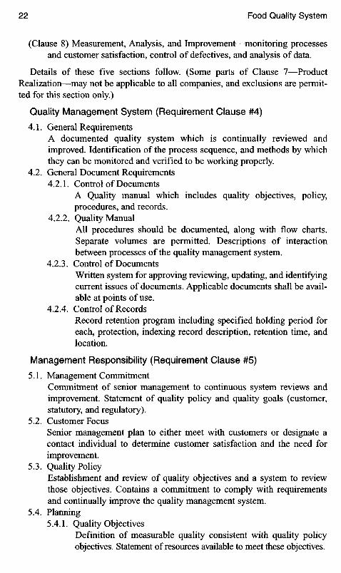
Quality Management System (Requirement Clause #4)
4.1. General RequirementsA documented quality system which is continually reviewed andimproved. Identification of the process sequence, and methods by whichthey can be monitored and verified to be working properly.
4.2. General Document Requirements4.2.1. Control of Documents
A Quality manual which includes quality objectives, policy,procedures, and records.
4.2.2. Quality ManualAll procedures should be documented, along with flow charts.Separate volumes are permitted. Descriptions of interactionbetween processes of the quality management system.
4.2.3. Control of DocumentsWritten system for approving reviewing, updating, and identifyingcurrent issues of documents. Applicable documents shall be avail-able at points of use.
4.2.4. Control of RecordsRecord retention program including specified holding period foreach, protection, indexing record description, retention time, andlocation.
Management Responsibility (Requirement Clause #5)
5.1. Management CommitmentCommitment of senior management to continuous system reviews andimprovement. Statement of quality policy and quality goals (customer,statutory, and regulatory).
5.2. Customer FocusSenior management plan to either meet with customers or designate acontact individual to determine customer satisfaction and the need forimprovement.
5.3. Quality PolicyEstablishment and review of quality objectives and a system to reviewthose objectives. Contains a commitment to comply with requirementsand continually improve the quality management system.
5.4. Planning5.4.1. Quality Objectives
Definition of measurable quality consistent with quality policyobjectives. Statement of resources available to meet these objectives.

5.4.2. Quality management system planningTop management shall ensure that resources are planned and iden-tified to meet requirements of quality system integrity.
5.5. Responsibility, Authority, and Communication5.5.1. Responsibility and Authority
Identification of key duties to ensure that responsibilities andauthorities of senior management and other department personnel aredefined and communicated. Organization structure informationshall make clear employee reporting system.
5.5.2. Management RepresentativeEmployee appointed by top management to oversee that processesneeded for quality management system are established, imple-mented, and maintained. Customer requirements promoted andsystem performance reported to top management.
5.5.3. Internal CommunicationCommunications are to report the effectiveness of the quality man-agement system.
5.6. Management Review5.6.1. General
Quality system review of current effectiveness and possibleimprovement. Shall include possible changes to quality policy andquality objectives.
5.6.2. Review InputSpecific process review
Audit resultsCustomer feedbackProcess performance and product conformityPreventive and correction action statusSystem changesRecommended improvement.
5.6.3. Review OutputSpecific output review
Effectiveness of management systemImprovement of product or servicesRequired resources for improvements.
Resource Management (Requirement Clause #6)
6.1. Provision of ResourcesProvide adequate resources to enhance customer satisfaction andimplement required and improved processes.
6.2. Human Resources6.2.1. General
Need for trained and experienced staff to perform indicated taskswhich affect quality. Evaluation of competence shall be evaluated onthe basis of education, training, skills, and experience.

6.2.2. Competence, Awareness, and TrainingThe organization shall determine personnel competence for workaffecting quality, and provide necessary training. Ensure that thepersonnel are aware of the importance of their activities.
6.3. InfrastructureProvide workplace, equipment, and employee service support.
6.4. Work environmentHuman and physical conditions managed for product and servicerequirements.
Product Realization (Requirement Clause #7)
7.1. Planning of Product RealizationEstablish product quality objectives and requirementsPlan all processes required for products and servicesPlan inspection and test proceduresIdentify reports and records related to product quality.
7.2. Customer-Related Processes7.2.1. Determination of Requirements Related to Product
Identify customer requirements for product or service, includinglegal requirements, delivery requirements, warranties (generally notapplicable to most food industries).
7.2.2. Review of Requirements Related to ProductDefine and record customer requirementsReview resource capability before accepting orderEstablish procedure for informing relevant sections of companyregarding requirement changes.
7.2.3. Customer CommunicationDefine customer procedure for communicating product informa-tion, such as complaints, inquiries, specification changes.
7.3. Design and Development7.3.1. Design and Development Planning
Identification of design, development and review stages.7.3.2. Design and Development Inputs
Identification of inputs relative to legal requirements, standards,safety, packaging, recycling, and labeling.
7.3.3. Design and Development OutputsDrawings, specifications: time, temperature, pH, concentration,bacterial levels, governmental regulations—all checked to insurethe product meets requirements.
7.3.4. Design and Development ReviewIdentify procedure and records for design review as developmentprogresses. Identify problems and propose necessary actions.Record progress. Maintain records of review stages.

7.3.5. Design and Development VerificationPlans to include methods for verifying that design meets require-ments. Records of the results shall be maintained.
7.3.6. Design and Development ValidationProduce product or service to establish that it meets requirements.Review customer feedback. Plans for further development.Records of the results of validation shall be maintained.
7.3.7. Control of Design and Development ChangesReview, verify, and record changes.
7.4. Purchasing7.4.1. Purchasing Process
Specifications of supplied material are clearly stated to supplier.Suppliers evaluated and selected on their ability to meet require-ments. Records of selection shall be kept.
7.4.2. Purchasing InformationPurchase order verification prior to sending to supplier. Includeproduct description, requirement for approval, quality managementsystem.
7.4.3. Verification of Purchased ProductReceiving inspection process. Procedure, documentation, recordretention.
7.5. Production and Service Provision7.5.1. Control of Production and Service Provision
Product characteristics specifiedTest proceduresTesting equipment and maintenanceAvailability of testing equipmentProcedures for release and delivery
7.5.2. Validation of Processes(Hardware industries oriented. Probably no application to foodindustry) Covers processes of monitoring and measurement afterproduct or service has been delivered.
7.5.3. Identification and TraceabilityManufacturing date and line code identification.Food industry—data for potential recall or shelf-life.
7.5.4. Customer PropertyHardware industry practice where customer supplies part for fur-ther processing and return as finished product. Procedures foridentifying, verifying and protecting product during operations.
7.5.5. Preservation of ProductStorage, identification, packaging, handling and stock rotation.
7.6. Control of Monitoring and Measuring DevicesIdentification of which tests need to be performed, and which test
equipment is to be used.

Maintenance and accuracy of devices—calibration and adjustment.Equipment safeguards against damage or deterioration.
Measurement, Analysis, and Improvement (Requirement Clause #8)
8.1. GeneralSpecify measuring and monitoring techniques to be utilized.Itemized list of statistical techniques.Process for continual product and process analysis and improvement.
8.2. Monitoring and Measurement8.2.1. Customer Satisfaction
Monitoring Customer Perception of Requirements.8.2.2. Internal Audit
Required to demonstrate system's ability to meet requirementsof ISO 9000.
Auditor is independent of process audited, competent tounderstand the process, and impartial.
External or internal auditors are acceptable.Define and document criteria, scope, and conduct of audits.
8.2.3. Monitoring and Measurement of ProcessesEstablish suitability of process and product control through
examination of product failures, customer complaints.8.2.4. Monitoring and Measurement of Product
In-process and final inspection procedures.Records of tests completed before delivery, with evidence of
conformity with acceptance criteria.Product or service release for delivery only if tests prove
satisfactory.8.3. Control of Nonconforming Product
Documented system for assurance that non-acceptable product is not usedin the process or shipped to customer. System to include procedures forremoving or retrieving faulty product.
8.4. Analysis of DataCollection and analysis of data to evaluate the quality system.Includes data from suppliers as well as customer satisfaction.Based on analyses, plans are made to improve.
8.5 Improvement8.5.1. Continual Improvement
Based upon quality reports, failure analysis. Analysis ofcustomer satisfaction and non-conformance.
Improve quality management system: quality policy, qualityobjectives, audit results, analysis of data corrective andpreventive action.
8.5.2. Corrective ActionIdentify, record, and repair problem areas.Evaluation of effectiveness of action taken.

Provide documented procedures to review nonconformities andcustomer complaints, causes of nonconformities, implementingaction needed, and recording results.
8.5.3. Preventative ActionEvaluate problems—actual and possible.Determine need for corrective action to eliminate causes of
nonconformities.Review and document effectiveness of corrective action.
MALCOLM BALDRIDGE NATIONAL QUALITY AWARD
The Malcolm Baldridge National Quality Award is presented by the President ofthe United States to a limited number of winners in manufacturing, service, andsmall companies each year. The primary purpose of the award is to recognize U.S.companies for business excellence and quality achievement. Additionally, theaward has encouraged thousands of organizations to undertake quality improve-ment programs. As mentioned in the previous chapter, the Malcolm BaldridgeNational Quality Award categories have undergone significant changes sinceinception. The early guidelines focused on the applicant's total quality system.After a few years, this was modified to recognize business excellence and qualityachievement. Either approach provides a useful format for evaluating and improvinga company quality system. However, it is suggested that companies use the 1990Baldridge Award Application Guidelines as a model if they are not yet satisfiedthat they have achieved a detailed and effective quality system. Category 5 of thisearly guideline, titled Quality Assurance of Products and Services, covers sevenof the basic requirements:
1. Design and introduction of quality products and services, emphasizinghow processes are designed to meet or exceed customer requirements.
2. Process and quality controls which assure that the products and servicesmeet design specifications.
3. Continuous improvement techniques (controlled experiments, evaluationof new technology, benchmarking) and methods of integrating them.
4. Quality assessments of process, products, services and practices.5. Documentation.6. Quality assurance, quality assessment and quality improvement of
support services and business processes. (Accounting, sales, purchasing,personnel, etc.)
7. Quality assurance, quality assessment and quality improvement of suppliers.(Audits, inspections, certification, testing, partnerships, training, incen-tives and recognition.)
Once a company is satisfied that an effective quality system has beenestablished, it might be desirable to examine the Baldridge Award criteria of

subsequent years to see if the goals of business excellence and quality achieve-ment are also being met.
TOTAL QUALITY MANAGEMENT (TQM)
TQM is more of a quality philosophy than a quality system. TQM is a goal inwhich every individual in every department of an organization is dedicated toquality control and/or quality improvement. In addition, this web of managementmay encompass suppliers and distributors as well. Some plans include thecustomers as partners in the quality efforts. Each organization has the freedom todefine "total," "quality," and "management" in any way they believe will enhancethe quality efforts within their scope.
One company instituted a program to train all of their employees with teamtechniques (see below) for solving quality problems and improving productquality. They referred to this activity as their TQM process.
Some companies have tried to avoid the stigma of reports of failed TQM pro-grams by using other terminology: "The Universal Way," "Quality ImprovementProcess," "Total Quality Service," "Quality Strategies," "Leadership ThroughQuality," "Total Systems Approach," "Quality Proud Program," "CustomerDriven Excellence," "Total Quality Commitment," "Total Quality Systems,""Statistically Aided Management."
Food Technology magazine, published by the Institute of Food Technologists,had several articles with widely varied definitions of TQM. One all-encompassingdescription of TQM states that it is a way of managing business, and is based onthe American Supplier Institute approach:
• Incorporate leadership, cooperation, partnerships, trust.• Aim for long-term goals of the business.• Concentrate on improving processes to improve results.• Deploy means and goals to all levels of the organization.• Use statistical quality control tools, quality function deployment, Taguchi
methods, and other quality tools.
Quality Progress magazine, a publication of the American Society for QualityControl, devoted an entire issue (July 1995) to 13 articles which described andevaluated TQM. Each paper was required to submit a brief definition of TQM.Table 2-1 indicates the differences of opinion between the authors.
The observation that there is no consensus for a TQM definition should notlessen its virtues. Applying as many quality control principles in as many areas aspossible is a desirable goal for any organization. Some companies have builtsuccessful TQM programs (using their own definition) by proceeding step wise;others have attempted to formulate the entire concept at once, and implement itin stages. There probably is no one best way.

Table 2-1. TQM System Components
Author's definitions
T Q M system components 1 2 3 4 5 6 7 8 9 1 0 1 1 1 2 1 3
Business or managementphilosophy
Continuous (mindset for)improvement
Continuous redesignedwork process
Customer focus/drivenCustomer/supplier
partnershipDelight customersDevelop improvement
measureDevelop with timeEmployee cooperationEvaluate continuous
improvementFailure mode effects
analysisGoal alignmentGuarantee survivalImprove customer
satisfactionImprove financial
performanceImprove management
systemImprove materials and
services suppliedLearning architectureMeet customers' needsMeet employees needsMeet owners' needsMission drivenPlan/do/check/actReduce costsReengineeringResponsible individualsResponsive customer serviceSelf-directed teamsSet targets for improvementStatistical process controlStrategic architectureTeamwork and trustUse of quality tools

TEAM QUALITY SYSTEMS
Teams generally represent a subsystem of quality control and improvementsystems. They rarely work well without a centralized quality control structuresince they are usually task oriented. Team concepts and operation will be coveredin some detail in Chapter 14.
COMPUTER NETWORK QUALITY SYSTEMS
Where operational cost/benefit analyses can justify the installation of computersystems on processing lines, opportunities for improved quality control accom-pany production gains. In addition to creating a system which can graphicallyshow current progress of every step of a process, track the quantities of ingredi-ents, supplies, work in process, and output, these same data signals can beharnessed to operate and control valves, burners, feeders, pumps, mixers andother equipment. Additionally, quality control can have the ability to use real-timedata for instantaneous control, to collect larger quantities of more meaningful andaccurate data, to provide high speed calculation and display of control charts,quality costs and other quality reports, and to instantly create and access datastorage. Computer systems are discussed in greater detail in Chapter 15.
SUMMARY
The many quality system approaches outlined in Chapter 1 are still used in thefood industry. There will never be complete agreement on the one best way, butrecent trends have emphasized the use of portions of the older philosophies, alongwith several new ones. Those considered most effective at present include thesystems explained above.
• Seven basic tools• Food processing industry quality system guidelines• Good manufacturing practice• ISO 9000 Standards• Malcolm Baldridge Quality Award• Total quality management• Team quality systems• Computer network quality systems.
Policy
A quality system is all but useless without an understanding of the company qual-ity policy. If the company policy on product packaging is to provide inexpensiveand functional sealed plastic film envelopes, then the quality control manager

might be doing the company a costly disservice to insist on precise printing andcolor control of these envelopes. A verbal understanding of policy is not enough.The policy should be in writing, signed by a company official, and reproduced asthe front page of the quality manual.
If a policy statement is unavailable, it may be difficult to obtain one becauseof organizational peculiarities or sensitive personal relationships between depart-ment managers. One of the more effective methods for generating a policy docu-ment is the preparation by the quality manager of a clearly labeled draft policywhich is forwarded to the company president for revision and approval throughwhatever channels are considered necessary. This provides the president with thenecessary guidelines, and still leaves him with complete authority to select thedetails.
A simple policy statement might read:
The Midwest Food Company is dedicated to supplying our customers with acompetitive quality line of standard products, and a superior line of choicequality products under the Gourmet label. All of our products shall be shelfstable for one year, safe, nutritious, and flavorful, and shall compare favorablywith the quality level of similar products found in our marketing area. They shallconform in all respects to the standards and regulations of federal, state, andlocal governments. The responsibility for quality control shall rest jointly withthe managers of purchasing, production, distribution, and quality control.
Major specifics might be included:
The Quality Control Department Manager shall establish and maintain productand process specifications. He shall be responsible for preparing and distributingroutine quality reports, exception reports, quality improvement reports, costreduction proposals, and shall perform monthly audits to evaluate all phases ofthe quality control system, including sanitation, product performance, house-keeping, and quality training. Quality control meetings shall be chaired weeklyby the Chief Executive Officer, and attended by managers and lead foremen ofall departments.
For some companies, more specific quality statements may be considereddesirable, but generally, the longer and more complicated a policy statement ismade, the less likely it will be read and followed. The details are best left forinclusion in the quality manual. Where there is likely to be a potential for misun-derstanding, it might be necessary for the policy statement to include the func-tional quality responsibilities for each department. The drawbacks to details ofthis nature are related to possible personality conflicts, turf battles, and restrictionof the contributions of capable employees.
Quality Control Manual
If a quality manual were prepared to conform to the best recommendations of allof the respected quality professionals, it would be so voluminous as to be useless.

And yet, it is essential that all of the critical elements of a manual be prepared,updated, and—most important—used. One suggestion to minimize the size with-out compromising the contents is to divide the manual into a set of numbered"submanuals":
MANUAL No. SUBJECTQl Policy, Organization, InterrelationshipsQ2 Research and Pilot Plant Quality ControlQ3 Material Quality ControlQ4 Production Quality ControlQ5 Product PerformanceQ6 Corrective ActionQ7 Microbiological ProceduresQ8 Packaging Material Test MethodsQ9 Product SpecificationsQlO Quality Audit ProceduresQIl Reports and FormsQ12 Government RegulationsQ13 Product Recall SystemQ14 Special Quality Requirements
An excellent guide to content and wording for an overall quality manual isMilitary Standard 9858A, obtainable from the Government Printing Office.Although it is hardware-industry oriented, it includes most of the basics and manydetails which might be overlooked.
The Secretary of Defense cancelled MIL Q 9858A as of October 1996, andadopted the ISO 9000 system in its place. The basic principles offered in MIL Q9858A are similar in most respects to the ISO 9000 standards, differing chiefly inthe following areas:
a. MIL Q 9858A has generally been the responsibility of the Quality ControlDepartment; whereas ISO 9000 cuts across organizational lines, requiringinput and responsibility from all departments.
b. ISO 9000 quality systems require constant review and modification.In fact the standard itself has a scheduled review and modificationrequirement.
c. ISO 9000 extends beyond the production quality concept, and includesproduct design. It also covers, as previously noted, a number of activitieswhich are more common to hardware manufacturers than food processors.
Test methods, other than those specifically listed above, may be includedunder other headings, or may be compiled into a separate manual. Primarily, thesetests are concerned with raw materials, process, and product. Additionally, samplesize, selection and frequency may be chosen from the above classifications,particularly if the techniques are complex. By preparing separate manuals to

cover such subjects as sampling and testing, training of new employees is oftensimplified.
Product Research and Development
From a legal viewpoint, one of the most important requirements in developmentof a new or improved product is documentation. This protects the company in theevent of patent or copyright litigation. For the scientist or engineer, accuratelyprepared records provide a route map for others to follow, and frequently suggestother developments for products, processing, or packaging to be explored at alater date.
Many creative food technologists prefer to work in an unstructured and infor-mal atmosphere, and for small companies or short-term projects, formalizedprocedures are not required. Guidelines are intended to assist workers, not to bindthem into a mold which restricts the inquisitive mind. Perhaps the systematizingof Research and Development (R&D) should be formalized more as an outlineor checklist, rather than as a rigorous procedure. This permits flexibility butprovides the safeguards which reduce the possibility of overlooking importantdevelopment steps.
1. Quality goal of R&D—The quality system should assure that specifica-tions are evolved which conform to marketing needs, manufacturingpractices, and regulatory requirements, and cover all aspects of materials,process, packaging, storage and use. These specifications might includethe following:• Physical and sensory properties• Product function and nutritive values• Process equipment and process rates• Packaging and packaging equipment• Composition• Microbiological limitations• Shelf life• Labeling and coding• Regulatory requirements.
2. Methods and standards—A checklist for methods and standards mightbest be considered as a flexible guide, since most developmental projectshave special requirements that will not fit a rigorous mold. To avoid thepossibility of overlooking important requirements, such a list should bereviewed at the start of any new development project:• Sampling and statistical analysis• Analytical testing methods• Calibration and maintenance of analytical equipment• Shipping tests and evaluation• Tolerance evaluation and review• Hazard and failure mode effect analysis

• Specifications for material, process, product, package• Consumer test design and evaluation• Patent potential evaluation• Outline of quality system for initial production• FDA, USDA, EPA, and local regulations.
3. Documentation—Progress reports usually are considered the basicdocuments for most development studies, and their presentation should bea planned procedure. Haphazard reporting may impede the efforts byrequiring disrupting staff meetings to explain the reasons for failures orthe direction of current research efforts. At the very least, milestonereports should be made (where applicable) at six stages:• Product concept• Prototype development• Pilot plant trial• Qualification testing• Field evaluation• Market readiness.
4. Reviews—Reports at the above six stages are intended to generate criticalreviews by involved personnel. A system should be evolved by whichcriteria for acceptance of progress can be established, permitting work toproceed to the next step. This should avoid unnecessary backtracking andinterruption of the research process. A universal checklist is impracticalsince each research project tends to be unique, but it is unwise to use thisfact as an excuse to avoid detailed documentation. Perhaps a master listfor qualification testing review might illustrate the scope of such a report.• Critical material• Product function and composition• Product stability—nutrient, sensory, function• Packing performance• Process variability• Process response—drift, interactions, errors• Shipping• Cost analysis.
Material Control
Over the years, "Just-in-Time" manufacturing systems have set goals to lowercosts by reducing inventories and eliminating rejects, rework and downtime byaccepting only defect-free raw materials in quantities no larger than those whichwere sufficient to keep the plant operating. Obviously, it is costly to producesatisfactory product from defective raw materials by sorting at the receiving dockor correcting on the line, and much effort has been made to assist vendors inproduction and delivery of defect-free field crops, food additives, and packagingmaterials. The key word here is "assist." The farmer may be unaware of thecritical nature of the sugar-acid ratio of his fruit in a jelly-making process. The

packaging film supplier may be unaware of the relationship of film thicknessuniformity and shelf life of a product. A fraction of a percent of gravel inunprocessed grain may abrade your raw material cleaning equipment. Byworking with suppliers, a manufacturer can often reduce the quality costs of bothparties. Improved materials reduce downtime, permit reduction of "Just-in-Case"inventories, and should improve profits.
Control of materials starts, at least theoretically, at the product developmentstage. It becomes a real consideration during supplier (also referred to as"vendor") selection, and eventually evolves into a daily consideration. Selectionmay be based on marginal criteria such as reputation, past performance, orreputation. Where material specifications are clearly written, they may eliminatesuppliers because of their inability either to reach or maintain the requirements.This should emphasize the need to be realistic when preparing specifications.They need not be more strict than is actually needed in the process, since this mayrule out alternate sources, and may often result in unnecessary added materialcost to achieve an unrealistic level of quality.
By working together, those responsible for quality control, for purchasing andfor production can work with their counterparts in the supplier's organization toprepare realistic purchase specifications and contractual requirements. With aclear understanding of the rules, suppliers may be willing to provide certificationdocuments with each shipment, thus avoiding the necessity for major incominginspection facilities at the processing plant. Under these conditions, suppliersmay also be willing to accept financial responsibility for production losses due toshipment of nonconforming raw material resulting in line stoppages, rejected orspoiled product, lost packaging materials, repacking, and overtime costs. This haslong been a practice for large-volume food processors, and should be equallyapplicable to smaller companies as well.
Assessing the quality of materials from suppliers should include:
• Inspection of supplier quality control program.• Evaluation of supplier specifications.• Examination of supplier facilities and production procedures.• Evaluation of performance through periodic audits.
Although one of the goals of supplier-purchaser relationships is the eliminationof incoming material inspection, it is unlikely that 100% achievement can beaccomplished without serious risk. For both attribute and variable inspectionplans commonly used, switching plans are available which permit reduced inspectionwhen a supplier has provided satisfactory material over a specified number oflots. This can substantially reduce the costs of material inspection while providingassurance that only useable material will be accepted. Ultimately, this might leadto a "Just-in-Time" supplier program, should this be considered desirable.
In the event of discovery of nonconforming incoming material, quality controlpurchasing and manufacturing departments should all be informed immediatelyto avoid the possibility of losses from production downtime or spoilage. Unless

properly controlled, rejected materials can find their way onto the productionfloor. The simplest of controls include four distinct steps:
1. Document the identification of the shipment, the inspection results,disposition recommended, and (when completed) final disposition.
2. Label nonconforming material clearly with distinctive markings andeasily read warnings not to use.
3. Segregate the shipment to prevent the possibility of mixing with satisfactoryproduct. If contaminated, isolate the shipment from edible storage areas.
4. Dispose of promptly. If destruction of the material is deemed necessary, itshould be observed by quality control personnel.
Under even the most satisfactory conditions, minimal receiving inspection isalways required for compliance with current FDA Good Manufacturing PracticesRegulations, other governmental regulations, and company policies. Supermarketchain stores and large food product distributors consider food processors as theirsuppliers, and are likely to require specific receiving inspection procedures at theprocessing plant as part of their overall quality systems. Regulatory or contractu-al considerations notwithstanding, it is always imperative to inspect at the receiv-ing dock for evidence of potential problems with sanitation, housekeeping, pestcontrol, adulteration or fitness for use. This represents a major departure from thepractices of the hardware manufacturing industries: the end-product of the foodprocessor is eaten!
Production Quality Control
The major eifort in quality control is devoted to the production line, and it mustbe designed around process capability studies. These will be discussed in detailin a later chapter. A process capability study determines whether the process canmeet the desired product specifications, where sampling points should be estab-lished, and the frequency of the sampling cycles. In addition, the direction forprocess change to improve quality and productivity is frequently highlighted duringprocess capability studies. The necessity for periodically conducting confirmingstudies is often overlooked. When a process is running comfortably in control fora period of time, a repeat process capability study may indicate the need for newcontrol limits, and perhaps new product specifications and new process targets.Normally, this is the basis for on-line product quality improvement.
It is next to impossible to continuously control a process without writtenprocedures. Word-of-mouth instructions from a supervisor to an operator areinvariably modified, misunderstood, or forgotten. Control cannot be accomplishedwhen a process operator explains his unusual procedures with excuses such as:"I've always found it works better this way"; or "I thought that is what I wasinstructed to do"; or "It didn't seem to be that important"; or, worst of all, "Nobodyever explained that to me." Documented procedures are difficult to establish,and they require continuous upgrading and correction; but they are essential to

providing a system which can be controlled to the same standards, day after day.A second major benefit from written procedures is their availability for providinguniform training to all new employees.
No one person should be required to take on the total responsibility for writingproduction operation procedures. They are less likely to be adhered to if they areforced onto the production department by an "outsider," even if they have beenprepared under the direction of top company management. To ease the introductionand acceptance of procedures, all affected supervisory or management employeesshould have the opportunity to review drafts as they are developed, and should begiven the responsibility for offering modifications to a draft before the finaldocument is issued for approval and use.
Occasionally one might expect management to balk at the concept of providingwritten procedures of proprietary operations to employees who might allow themto fall into the hands of competitors. It may be possible to alleviate these fears bythe use of codes for critical temperatures, pressures, flows, or special equipment.Or where possible, such critical data might be left blank on the procedures, butposted on the equipment for use by the employee. It is not unusual for employeeswith proprietary process knowledge to leave one company, with or withoutdocuments, for employment with a competitor. Nevertheless, the advantages ofwritten process procedures far outweigh the disadvantages.
Control of operations may include several functions, such as:
1. In-process inspection of materials, product, and package.2. Process verification.3. Status identification of raw materials, partially processed and finished
product (ordinarily performed by use of a tag system; see Figure 2-1.)4. Test equipment calibration. This would include meters, gages, media,
reagents, metal detectors, check-weighers, production instrumentation, etc.
Figure 2-1. Suggested forms for controlling reagent standardization andfor controlling nonconforming materials.
MECORPREAGENT
DATE REC1D
TEST DUE TEST RUN OK' BV
LOT NO:
SUPPLIER:DATE REC1D
REASON REJECTED
LOCATION
DATE RETESTEDDISPOSITION
SIGNED QC DEPT
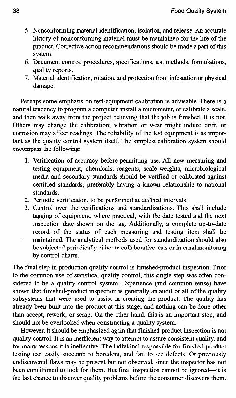
5. Nonconforming material identification, isolation, and release. An accuratehistory of nonconforming material must be maintained for the life of theproduct. Corrective action recommendations should be made a part of thissystem.
6. Document control: procedures, specifications, test methods, formulations,quality reports.
7. Material identification, rotation, and protection from infestation or physicaldamage.
Perhaps some emphasis on test-equipment calibration is advisable. There is anatural tendency to program a computer, install a micrometer, or calibrate a scale,and then walk away from the project believing that the job is finished. It is not.Others may change the calibration; vibration or wear might induce drift, orcorrosion may affect readings. The reliability of the test equipment is as impor-tant as the quality control system itself. The simplest calibration system shouldencompass the following:
1. Verification of accuracy before permitting use. All new measuring andtesting equipment, chemicals, reagents, scale weights, microbiologicalmedia and secondary standards should be verified or calibrated againstcertified standards, preferably having a known relationship to nationalstandards.
2. Periodic verification, to be performed at defined intervals.3. Control over the verifications and standardizations. This shall include
tagging of equipment, where practical, with the date tested and the nextinspection date shown on the tag. Additionally, a complete up-to-daterecord of the status of each measuring and testing item shall bemaintained. The analytical methods used for standardization should alsobe subjected periodically either to collaborative tests or internal monitoringby control charts.
The final step in production quality control is finished-product inspection. Priorto the common use of statistical quality control, this single step was often con-sidered to be a quality control system. Experience (and common sense) haveshown that finished-product inspection is generally an audit of all of the qualitysubsystems that were used to assist in creating the product. The quality hasalready been built into the product at this stage, and nothing can be done otherthan accept, rework, or scrap. On the other hand, this is an important step, andshould not be overlooked when constructing a quality system.
However, it should be emphasized again that finished-product inspection is notquality control. It is an inefficient way to attempt to assure consistent quality, andfor many reasons it is ineffective. The individual responsible for finished-producttesting can easily succumb to boredom, and fail to see defects. Or previouslyundiscovered flaws may be present but not observed, since the inspector has notbeen conditioned to look for them. But final inspection cannot be ignored—it isthe last chance to discover quality problems before the consumer discovers them.

Finished-product testing can include examination for whatever attributes areincluded in the specification, but the crucial test should be performance of theproduct. The product should look, smell, dissolve, and taste right. It should betested in the same manner as the customer or consumer would normally use it. Ifit is a teabag, the paper should not disintegrate in the cup—the customer is notinterested in the number of grams offeree required to separate the seam, but onlythat the tea leaves remain inside the bag.
Another class of finished-product inspection is acceptance testing to assurethat production lots have met quality requirements. This may be accomplishedeither by 100% testing or by lot sampling, to be discussed in Chapter 5.
Storage, handling, and shipping may adversely affect the quality of foodproducts, with the possible exception of some wine and cheeses. Lengthy storagepermits settling of some emulsified liquids, and may be responsible for damagefrom corrosion, infestation, or degradation. Damage from improper handling andshipping would include leaking or deformed containers, scuffed labels, or crumbledproduct. Abnormally high-temperature storage of "commercially sterile" cannedgoods may result in thermophilic bacterial spoilage. Temperature control duringstorage of frozen or refrigerated products may be critical. Control of the qualityduring this phase of the product life starts with audit of shipping procedures andof stored items. Systems development for storage, handling and shipment generallyrest with the distribution manager, but quality problems associated with theseareas can be highlighted by quality control personnel, and perhaps some suggestionsfor quality improvement may be uncovered and suggested.
Product coding and case marking may seem like a simple housekeeping chore,but it can assume monumental proportions in the event of a product recall.Whether the problem in a recall is relatively small, such as forgetting to includea minor ingredient in a short run, or accidentally labeling the orange-flavoredproduct "mandarin orange flavored," or whether it is a major product quality failure,proper coding can mean the difference between calling back a truckload or twofrom a small area, or bringing back product from the entire distribution area formany days of production because the code could not be identified.
Governmental requirements for coding are the minimum to be considered. Ifpossible, all information should be included in codes: date, shift, line and plant oforigin, plus batch, and product description. By the use of the Julian Date Code(the number of the day in the year) and a combination of letters and colors, a greatdeal of information can be inserted in small space. The month of the year can bedesignated as 1 through 9 for January through September, and the last threemonths might use either O, N, D or inverted 1,2,3; and the year could be expressedas a single digit; thus the date portion of the code need not exceed five characters.Universal product codes, label edge scoring codes, and other ingenious schemesmight also be used where they do not conflict with regulations.
Finally, production quality records shall be considered. Since these tend tobecome voluminous in a short time, some procedures need to be established forretaining only those records which are actually useful. The general rule is to retainrecords for no longer than the normal life of the product. It is strongly suggested

that this rule be modified somewhat. In order to retain skeletal data for use incomparing product quality progress over several years, and to retain records ofprior formulations and methods in the event they may some day be used again,one scheme retains all records selected at random from one day per month for aperiod of one year after the normal product life, and then reduces older recordsby selecting at random one month per year for retention for two years. If thesequality records are retained in a computer, there is no reason to destroy any ofthem, since they may be stored on inexpensive disks. But if the records are onpaper, a system such as the one described is recommended. Following is aschematic representation of the records retention system for a product withmaximum life of two years.
The goals of a quality records retention system need to be clearly establishedif they are to be effectively reached (Table 2-2). And there are many such goals:
1. Provide evidence that prescribed tests and inspections were made.2. Identify personnel responsible for performing quality tasks in the event
that they need to be questioned.3. Accumulate rejections, scrap and rework data for calculations of quality
costs (for cost reduction efforts).4. Identify product, and trace materials, equipment, operations, and date of
production.5. Establish database for providing reports to management of quality
performance, action taken, and recommendations for product, materials,process or cost improvement.
As with any system, success is based upon effective management. Unless thequality manager constantly reviews the goals of his programs, and takes action,when necessary, they tend to be overlooked, dooming the quality function tothat of a paperwork generator. This no more apparent than in the collection ofquality records. They contain much valuable information but, to be of use to the
Table 2-2. A Records Retention system
Year
12345567
Completefile
11,22,33,44,55,66,77,8
Retain one day's filesper month for year no
11,22,33,44,55,6
Permanent fileone day per year
11,2
1,2,31,2,3,4
company, they must be studied, analyzed, and reported in digest form withrecommendations for constant productivity improvement.
Departmental Relationships
The quality control system cannot function in a vacuum. It must be integrated intothe entire fabric of the company. Unfortunately, there is no magic formula toaccomplish this. Cooperative relationships between departments cannot beexpected to operate because of a presidential edict, and there is little to be gainedby writing such relationships into the quality manual. In fact, telling otherdepartments how to function is bound to feed some amount of antagonism into acompany. The amount may be significant, or it may be negligible, dependingupon personalities of those involved, And here is the heart of the matter. A foodprocessing company is often thought of as a steel arid concrete building, filledwith noisy equipment and fragrant vapors, fed by truckloads of raw material andgenerating truckloads of finished product. It certainly is more than that: it func-tions only because there are people within it—all with diverse personalities,needs, intellectual abilities and goals. Men and women are all prone to jealousiesand anger, pride and despair, energy and lassitude, ambition and despondency,cooperativeness and selfish independence.
Is it possible to create a quality policy which will lead all of these individualsinto one common direction? Perhaps so. If it is true that only management cancreate a system under which quality control works, then it would seem logicalto expect that a system could be evolved in which all departments participateto contribute to quality control. The following oversimplified example mightsuggest a way around the problem.
Let us consider a company in which the purchasing department is expected tosupply the production line with least-cost packaging material. In the same company,the quality control department is expected to control the quality of the packagingat some predetermined level. Finally, the production department is expected tokeep the packaging lines operating without interruption in order to minimizecosts, eliminate a second shift or overtime. If, under these suppositions, purchasingsupplies inexpensive but unreliable packaging, production will suffer numerousdowntime episodes because of malfunction of the packaging material, and qualitycontrol will reject vast quantities of substandard production, thus requiringproduction to schedule additional shifts to make up for lost product. Each depart-ment, exclusive of the other two, may have done its job in exemplary fashion, butthe total effort was a costly quality failure.
No amount of arguments between the departments will alleviate the problem.No department can be expected to tell another department how to run its affairswithout adding to the conflict. Now let us bring enlightened management into thepicture. If the company president decides the time has come to correct these costlyproblems, he might arrange a solution which overcomes the special needs ofthe individual departments. Purchasing, quality, production, and finance shallmeet once each week to select jointly a packaging supplier whose material cost

and quality level would result in the highest output, at the specification qualitylevel, and at the least cost. We now have a system of purchasing packaging mate-rials which overcomes personalities and departmental goals. This is a companygoal-oriented system, and has a far better chance of success.
The problem and its solution have perhaps been oversimplified. It might, forexample, be worthwhile to include other departments such as research orengineering to consider alternative package design or production methods orequipment which might use cheaper packaging material successfully. The principleof management systems is a valid one, however. It is equally applicable to theproduction, shipping, commodity procurement, and possibly personnel depart-ments. It cannot completely overcome personality conflicts, but it can controlthem to a large extent.
This chapter is directed at the quality control department, not the president ofthe company. So far it has not supplied the quality manger with a solution to theconflicting departmental goals. Teaching quality control methods to the companypresident can only be accomplished in small steps, since his priorities are usuallydirected elsewhere; but small steps are certainly not undesirable.
It would be a near miracle to provide a company with a new and effective com-plete quality control program in a single step. However, one can be developed inphases. If, in the example above, the purchasing manager could be approachedand shown how he could become a company hero by reducing the costs due topackaging problems on the line, then the first step toward interdepartmental qual-ity operations would be launched.
In a similar fashion, solutions to quality problems on the line which arediscovered through analysis of quality reports can be discussed with managementin other departments for their corrective action. This will assist in cementingrelations with the quality department and in gradually developing the company-wide quality team approach, frequently referred to as "total quality control."
Product Performance
The objective for a company is to make a profit. The objective for the manufactureof a product by that company is to satisfy the consumer's needs and expectations.The consumer provides the final—and most important—audit of the productquality, and contact with the consumer by the quality control department is theonly way to really understand if the product quality is satisfactory. The contactsmay be direct through form letters, coupons, mailings, or meetings. These tech-niques may be administered by outside consultants, internal sales and marketingdepartments, or by quality control.
Whenever practical, potential users of a proposed new product should becontacted to determine its intended use and practical requirements. Once a product isin the market, care must be taken to review dissemination of product informationto the public. It should reflect the needs of the consumer, as well as truthful

representations of the performance, quality and safety. The advertising should bereviewed for accuracy and conformance to regulations. Statements such as "twicethe strength," "instantly soluble," "will keep forever in an unopened container,""sugar-free," "preferred by 80% of the product users," "organically produced,""reduced calories," and "guaranteed fresh" all require supportable evidence fromthe technical staff of either the research department or the quality control depart-ment. The quality system should provide the mechanics for reviewing marketingstrategies where such advertising is proposed.
If nothing else, contact with the consumer in the form of a consumer complaintmust be handled quickly and with care. It has been claimed that a single consumercomplaint may represent somewhere between 20 and 200 other consumers whohad the same negative experience, but merely changed brands rather than writingto the manufacturer. Each company may have its own preferred procedures forresponding to the complaint, but in all cases, a copy of the complaint and the responseshould be forwarded to quality control so that efforts to prevent recurrencescan be started immediately. Complaints may fall into many differentcategories, depending upon the product. They may be concerned with flavor,odor, foreign material, appearance, net volumes or net weights, presumed healtheffects, deterioration, etc.
Complaints which fall within the product specification may be classified asnuisance complaints, and handled by replacement of product to the consumer.Where a product has apparently been produced outside of specifications, attemptsshould be made to obtain the package code date so that an immediate investiga-tion can be performed. Remembering the 20 to 200 unwritten complaints (seeabove), this one might represent a serious quality problem, perhaps even a recall.Finally, where a product complaint indicates health hazards, all informationshould immediately be turned over to the company's insurance handler or legaldepartment. No direct contact with the customer by other company personnel isadvisable because of possible legal liability considerations. However, close contactbetween technical and legal is essential in order to establish the facts quickly.
Individual responses to consumer complaints are not the end of the story.Complaints should be compiled into categories by month, and cumulative for thepast 12 months (do not use cumulative data for the current calendar year—thiscan be misleading). The data should be listed by number of complaints and bypercent. If the company is unfortunate enough to have a large volume ofcomplaints each month, control charts can be constructed to highlight both trendsand emergencies. In any event, use of percentage figures will highlight unusualsituations. All data should be considered confidential, and not distributedthroughout the company except as required. A sample of such a compilation(from a fictitious company) is shown in Table 2-3.
An improvement over simple tabulation of complaints would be to include thesales figures as well as the complaints. Graphs showing types of complaints byproduct by month along with the number of units sold during that period mayshow that seasonal increases in complaints are accompanied (adjusting for lead
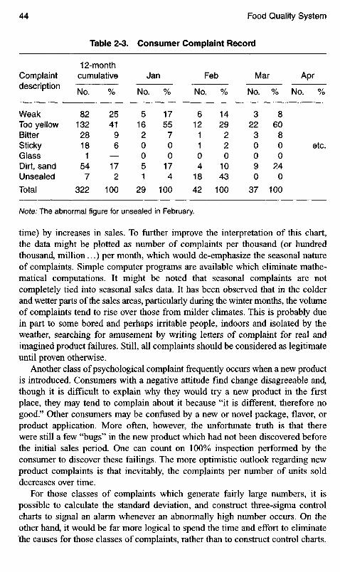
time) by increases in sales. To further improve the interpretation of this chart,the data might be plotted as number of complaints per thousand (or hundredthousand, million...) per month, which would de-emphasize the seasonal natureof complaints. Simple computer programs are available which eliminate mathe-matical computations. It might be noted that seasonal complaints are notcompletely tied into seasonal sales data. It has been observed that in the colderand wetter parts of the sales areas, particularly during the winter months, the volumeof complaints tend to rise over those from milder climates. This is probably duein part to some bored and perhaps irritable people, indoors and isolated by theweather, searching for amusement by writing letters of complaint for real andimagined product failures. Still, all complaints should be considered as legitimateuntil proven otherwise.
Another class of psychological complaint frequently occurs when a new productis introduced. Consumers with a negative attitude find change disagreeable and,though it is difficult to explain why they would try a new product in the firstplace, they may tend to complain about it because "it is different, therefore nogood." Other consumers may be confused by a new or novel package, flavor, orproduct application. More often, however, the unfortunate truth is that therewere still a few "bugs" in the new product which had not been discovered beforethe initial sales period. One can count on 100% inspection performed by theconsumer to discover these failings. The more optimistic outlook regarding newproduct complaints is that inevitably, the complaints per number of units solddecreases over time.
For those classes of complaints which generate fairly large numbers, it ispossible to calculate the standard deviation, and construct three-sigma controlcharts to signal an alarm whenever an abnormally high number occurs. On theother hand, it would be far more logical to spend the time and effort to eliminatethe causes for those classes of complaints, rather than to construct control charts.
Complaintdescription
WeakToo yellowBitterStickyGlassDirt, sandUnsealed
Total
1 2-monthcumulative
No.
8213228181
547
322
%
2541
96
172
100
Jan
No.
5162OO51
29
%
17557OO
174
100
Feb
No.
612
11O4
18
42
%
1429
22O
1043
100
Mar
No.
322
3OO9O
37
%
860
8OO
24O
100
Apr
No. %
etc.
Note: The abnormal figure for unsealed in February.
Table 2-3. Consumer Complaint Record
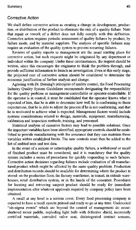
Corrective Action
We shall define corrective action as creating a change in development, produc-tion, or distribution of the product to eliminate the risk of a quality failure. Notethat repair or rework of a defect does not fully comply with this definition.Corrective action requires periodic assessment of quality failures by product, byfailure mode, and by material suppliers. The analysis of specific failures mayrequire an evaluation of the quality system to prevent recurring failures.
Reviews of quality reports to management are the usual starting place forcorrective action, but such requests might be originated by any department orindividual within the company. Under these circumstances, the request should bewritten, since this encourages the originator to think the problem through, andprovide sufficient information to launch an investigation. Even at this early stage,the projected cost of corrective action should be considered to determine theeconomic justification of further analysis and change.
Agreeing with Dr. Deming's principles of quality control, the Food ProcessingIndustry Quality System Guidelines recommends designating the responsibilityfor the quality problem as management-controllable or operator-controllable. Ifthe operator is in control, it must be established that the operator knows what isexpected of him, that he is able to determine how well he is conforming to thoseexpectations, that he is able to adjust the process if he is not conforming, and thathe is motivated to achieve what is expected. Management factors would includesystems considerations related to design, materials, equipment, manufacturing,calibration and inspection methods, training, and personnel.
Statistical analysis of causative factors may lead to possible solutions. Oncethe important variables have been identified, appropriate controls should be estab-lished to provide manufacturing with the assurance that they can maintain thosevariables within established limits. The new controls must then be added to thelist of audited tests and test data.
In the event of a serious or catastrophic quality failure, a withdrawal or recallof finished product must be considered, and it is mandatory that the qualitysystem includes a series of procedures for quickly responding to such failures.Corrective action decisions regarding failures include evaluation of all manufac-tured product which might be affected by the same quality problem. Productionand distribution records should be available for determining where the product isstored: on the production floor, the factory warehouse, in transit, in outside ware-houses, retail distribution system, or in the hands of the consumer. Proceduresfor locating and retrieving suspect product should be ready for immediateimplementation after whatever approvals required by company policy have beenobtained.
A recall at any level is a serious event. Every food processing company isexpected to have a recall system primed and ready to go at any time. Undetected"six-sigma events" which are beyond the control of management do occur:shattered mixer paddle, exploding light bulb with defective shield, incorrectlycertified materials, corroded valve seat, disintegrated contact sensors,

atmospheric contamination, and even sabotage. This is the one program, morethan any other, which must be formalized, documented, and maintained current.Considerable assistance is available to set up such a program. The Code ofFederal Regulations Number 21, Part 7, covers FDA regulations. The ConsumerProduct Safety Commission, CPSC Act 1972, Section 15 also refers to recalls.The Grocery Manufacturers of America, Washington, DC has published an excel-lent pamphlet which describes a recall system for food products. Once a systemhas been established, it should be periodically tested by performing a mock recall.This will quickly verify that either the system is workable, or that there aredeficiencies in either the system or in the record keeping procedures in variousdepartments, or perhaps in outside warehouses. These deficiencies must beimmediately remedied, and tested again at a future mock recall.
Company policies differ on the desirability of written reports of quality failures,such as recalls. Some companies may prefer that no written material be prepared;others use recall records as training materials for certain employees. It issuggested that those responsible for company legal matters be consulted on thismatter. A concise report covering steps taken in the event of a recall may berequired by the legal representative as defense material to be used, should litigationarise as a result of product quality failure.
Quality Personnel
In classical industrial engineering system studies, the four "ms" considered aremen, materials, methods, and money. So far in this discussion of quality systems,we have only considered the last three items. And yet, the best quality system willnot function without people who are carefully selected, trained, and motivated.Regardless of which department is responsible for recruitment of quality controlpersonnel, the responsibility for identifying the characteristics of a satisfactoryquality employee must be assumed by quality control management. Qualitycontrol need not be staffed by the same type of outgoing and personable individ-ual required by, for example, the sales department. Nor should the qualificationsrigorously insist on the often mistaken need for a stereotype of an unbendingpolice-type. Such character traits as dedication and honesty are required, alongwith alertness and a proficiency in at least basic mathematics. Mechanicalaptitudes are often useful as well. The process for recruitment and selection ofemployees differs from company to company, but the final approval shouldalways remain with the quality manager. Vacancies may be filled by promotingfrom within, reviewing resume files, newspaper and trade journal advertising,employment agencies, and other channels. Consequently, the manager is expectedto have a list of candidate employee qualifications available for guidance. Thefinal selection of employees should be based on their capability and experience,or their potential to qualify for the job.
Large corporations may have training departments which can quicklyindoctrinate a new employee with company policies and procedures. Large orsmall, however, a company quality manager is still responsible for training new

employees in their new assignment. Company policies and procedures manualsare useful for training newcomers to any department. The special trainingrequired for quality department newcomers is highly specialized. It must begeneral in nature, but at the same time, specifically oriented to the company'soperations and quality policies. Study of the quality manuals is perhaps the quickest(and most uniform) method for training quality control personnel. Quality controlpersonnel from other industries may not be aware of the critical nature of qualityin the food industry. If a lawn mower is delivered with its blade's cutting edgesinstalled backwards, it can be repaired or returned for replacement. Not so withfoods: if a food product contains a major defect which might affect the health ofthe purchaser, it cannot be repaired , and might cause serious consequences.Many hardware industries deal with slow production lines of expensive productswhich are controlled by indirect nondestructive test methods; most food processingplants operate high-speed processes, requiring different quality testing techniques.All quality employees should be required to take refresher courses geared tointroducing new concepts and to the eradication of complacency, and eliminationof "short cuts."
The need for training of line and supervisory employees in the principles ofquality performance is best handled by personnel other than those from qualitycontrol. The production employee would willingly agree that the principles ofquality workmanship would make the quality control department "look good."But at the same time, the possibility of reducing production rates by using care-ful and precise quality methods might make the production line supervisor "lookbad." Of course this is not necessarily true, but the problem exists, nevertheless.By utilizing trainers from other departments, or from outside the company, thisapparent conflict is reduced. Obviously, the best control of quality performance isachieved when both the production personnel and the quality control personnelare all effectively trained in the principles of quality effort.
Motivation is another key to the success of quality control, and there is no oneformula for providing this tool. It is important for quality employees to under-stand the consequences of a slip-shod performance. It is equally important for theline and supervisory personnel to be aware of this. A thorough knowledge of theprinciples of quality effort, as mentioned above, is required for quality control;but without the motivation to actually perform under these principles, the resultswill be less than acceptable. Motivational tools are numerous, and many areeffective. Unfortunately, most are short-lived, and when applied a second time,there is frequently a disinterest, or even an antagonism exhibited on the part ofthe employees. There is one motivational tool which seems effective in practicallyall situations: recognition of achievement. How this is best applied must be care-fully thought out. Setting up a reward system consisting of a dinner with the plantmanager may work once or twice, but it may not be considered a reward by many.Worse, it is difficult to bring the program to an end or to replace it with anotherreward. (And this hardly considers the plant manager's long-term feelings aboutsuch an arrangement.) Recognition can be as simple as a kind word from thecompany manager to an employee at his workstation. Financial awards,

vacations, promotions, pronouncements at the Christmas Party or in the companynewspaper, plaques, gifts, posters—these are some of the many ways torecognize efforts and to provide motivation, some of which are more effectivethan others. Whatever method is selected, it should be made clear to the recipientand all of his fellow workers that the award is made in recognition of outstandingperformance—it definitely is not a bribe to do the job correctly.

3 Control Charts
THE IMPORTANCE OF CHARTING
The ancient saying, "one picture is worth a thousand words," is somewhattime-worn, but far from worn out. In a world where statistics and columns ofnumbers are not well understood, a picture of a process may be far easier to graspthan a quality summary laced with standard deviations, averages, equations, andnumerical computations. The control charts used in statistical quality controlrepresent a picture of a process. When used and continuously updated on theproduction floor, charts represent a moving picture of the process.
The frequent misuse, or occasional fraudulent misrepresentation of charts andgraphs, has placed them under suspicion. For one example, let us suppose we areconsidering the increase in the cost of changing raw product for a process fromstandard grade to choice. In preparing a report on this project, a simple bar chart(Figure 3-1) may be used to compare the cost in 1998 and the cost in 2003 whenthe new material is intended to be used. The dollar column on the left of the chartbelow represents the 1998 cost; the column on the right shows the year 2003 costat about double the amount.
To emphasize the difference, we may choose to represent the increase in costsby a three-dimensional picture. Here, as before, the vertical stack height of theyear 2003 is double the height of the 1998 dollars, but by doubling the depth and
Figure 3-1. Bar chart comparing costs for two years.
1998 2003
$

width as well, the appearance of the new costs is dramatically (and untruthfully)magnified. The year 2003 dollars are not the same dollars as those of 1998(Figure 3-2).
Another commonly used trick of reaching unwarranted conclusions by manip-ulating graphs is the magnifier principle, frequently practiced in newspapers toprove a point. Although it might be useful occasionally, extreme caution shouldbe taken when employing this technique. For example, in Figure 3-3 the leftgraph shows the level of petty cash in an office safe over the years. The enlargedgraph on the right has selected the most recent week with grossly magnified axisvalues, suggesting that petty cash is skyrocketing. In truth, it is most likelyfluctuating in the general range where it has wandered over the past few years.
Figure 3-2. Three-dimensional diagram exaggerating costs for year2000.
1998 2003
DetailDollars Dollars
Petty cash This Week
Figure 3-3. Misleading effect of an enlarged portion of a chart.
1975 1980 1985 1990 Mon Tu* W*d Thur FH Sat

Figure 3-4. Misleading effect of a pie chart.
Pie charts (Figure 3-4) may be used to represent percentages or portions of apopulation, and are sometimes useful. They are difficult to interpret if manysections are shown, and they can be misleading if they are portrayed in three-dimensional perspective. Note in Figure 3-4 how a 15% portion in the front ofthe pie can emphasize the profit of a proposal in the left pie slice; by contrast,note how the same 15% placed in the rear of the pie (and with a change in typesize and font) suggests that the costs of this proposal are prohibitive compared tothe meager profits.
On the other hand, charts and graphs are valuable tools for presenting statisti-cal data. Of particular interest are the control charts used universally to presentquality data. They are sufficiently simple to interpret so that misunderstandingsare avoided. Regardless of the type of control chart, they all contain a few funda-mental characteristics (Figure 3-5). They contain upper and lower control limitswithin which all observations will lie if the process is in control. They contain acenter line which is usually considered to be the target value for the process. Andthey generally show numbers along the vertical axis to define the values of thecontrol limits and of the observations. Beyond these basics, the charts may be tai-lored to suit the requirements of the operation.
If one were to ask for the basis of statistical quality control, there might beconsiderable discussion; but the X-bar and R chart would rate very high on thelist. These two charts are easy to prepare, simple to understand, and extremelyuseful in locating problems and even in suggesting possible solutions. They areideal tools for discovering ways to improve product quality and process control,and they can drastically reduce scrap and rework while assuring the production of
PROFIT
COST
profit
or
cost
THE PIECHRRTGRME

Figure 3-5. Characteristics of a control chart.
only satisfactory product. They are used for controlling every step of a produc-tion process, for the acceptance or rejection of lots, for product improvementstudies and for early detection of equipment or process failures. An example ofan X-bar control chart taken from an orange-flavored dry drink mix packagingline at the filler discharge shows the citrate concentration as determined periodi-cally by the quality control laboratory (Figure 3-6). (The average line has beenomitted for clarity.) At nine o'clock, a point appears just above the control limit.Since, by chance alone, this may happen as infrequently as three times per thou-sand observations and still represent a process in control, no action is indicated.As the chart subsequently shows, the next few points are indeed within limits, andthe process is allowed to proceed. At 12 o'clock, another point is out-of-limits,and the recheck point immediately following shows, without doubt, that theprocess is far out of control. The line was stopped, and it was determined that anoperator had inadvertently dumped a drum of lemon drink mix into the hopperduring the noon shift relief change. The citrate control limits for the lemon mixproduct are 6 to 8 units, which would explain the increase. Additional subsequentevidence obtained by the laboratory confirmed the mistake by product coloranalysis, and flavor evaluation.
In addition to X-bar and R charts, a group of charts loosely defined as attrib-ute charts are used for control of defect analysis. They are particularly useful forcontrolling raw material and finished product quality, and analyzing quality com-ments in consumer letters. An attribute is a characteristic of a product, a process,or of any population, which can be counted or tallied, but which otherwise can-not be described in incremental numbers. It would be more meaningful to definean attribute as a characteristic which is either satisfactory or unsatisfactory; go-or-no-go; defective or nondefective; good or bad; heavy or light; etc. The onlynumbers which can be applied are the number or percent of the satisfactory orunsatisfactory units. These charts (which will be considered later on) are thep charts (fraction or percent defective), np charts (number of defectives), and c oru charts (number of defects). First, we shall explore the X-bar and R charts.
To start with, the X-bar and R charts are used for control of variables. Variablesare measurements which are expressed in discrete numbers: inches, pounds, pHunits, angstroms, percent solids, degrees centigrade, etc. In the case of a leakingcontainer, a variable measurement would be the rate at which gas flows throughthe leak in cubic centimeters per hour. An attribute measurement, on the other
Upper control limit
Target (or Average)
Lower control limit
Measurement

ORANGE DRINK MIX
Figure 3-6. X-bar control chart for orange drink mix.
hand, would be the number of leakers or nonleakers in a batch or in some timeperiod.
Jf-bar is usually written as X, and is the average value of several measure-ments, each of which is called X9 and generally identified by themeans of subscripts: X^ X2, X3, etc. As we shall learn later (in Chapter 4,Fundamentals), some distributions of data may be lopsided (skewed) because ofpeculiarities of the process from which the data has been obtained. It will also beexplained that taking averages of data from a process, regardless of the distributionof the data, tends to reduce these irregularities, resulting in a smooth distribution.Hence, a graph of a series of JT-bars shows a smoothed representation of theprocess being measured. This makes it easier to determine when the process is outof control, since smoothed data will lie in a relatively narrow range.
A possible weakness of an X chart is that individual points on it are repre-sented by averages of data which might contain wide ranges of values, but whichare masked by the very smoothing effect that makes these charts so desirable. Toovercome this difficulty, the range of data from which each average was obtainedis also required, and in turn, its control values (upper and lower) must also becalculated.
PROCEDURE FOR CONSTRUCTING X-BAR AND R CHARTS
The preceding verbose description is a good argument for the statement that apicture is worth a thousand words. With that in mind, we shall proceed to constructan actual control chart (Figure 3-7). A first example will be a control chart forheadspace in one-pound jelly bean jars packed on one of the six lines in the plant.Our concern is that insufficient headspace is likely to crush the product when thelid is applied, and that excess headspace will allow the product to abrade duringtransport. Experience has shown that a headspace of about 3/32 or 4/32nds of aninch is satisfactory, but plant operating people are not certain of what any of thelines are capable of producing. We will work with Line #3 to start. A preliminarychart can be prepared from about 100 headspace measurements. For a more
Time
X CONTROL CHART
Citrate
UCLx
LCLx

realistic working chart, it is customary to obtain 30 subgroups of five samplesfor a total of 150. (Refer to the data and calculations in Table 3-1 as we go throughthe following steps.)
1. When Line #3 is operating satisfactorily, select about 100 jars off the linebefore the lids are applied. All jars must be selected in sequence, and keptin order until measured.
2. Measure the headspace in each jar, in order, and record in groups of five,as shown in Table 3-1. (Sample 1 measures 7/32, and is recorded in thefirst column as "7." Sample 2 measures 10/32, and is recorded in the sec-ond column as 10. Continue until reaching sample 6, which measures6/32 and is recorded in the first column under the first sample taken.Eventually 16 rows of five columns will be completed. This totals 90 sam-ples—close enough to the 100 generally required for a first attempt. Thereason for the five columns will be explained shortly.
Sample number
1 2 3 4 5
7 10 8 2 86 9 3 4 36 7 2 6 44 8 5 7 7
1 0 3 5 6 48 11 9 6 65 7 5 6 79 5 8 7 66 5 4 5 51 3 1 0 33 4 6 5 45 3 6 3 35 6 8 9 77 7 8 7 67 7 6 7 77 7 7 9 9
(add columns) Totals(divide by 16) Averages
Average (X)
7556.25.686751.64.84776.87.8
93.85.86
Range (R)
8654752423334212
613.81
A2 for sample of 5 = 0.577D4 for sample of 5 = 2. 11 5 (from tables)D3 for sample of 5 = O
Table 3-1. X-bar and R Chart Calculations.Headspace—One Pound Jelly Bean. Line No. 3
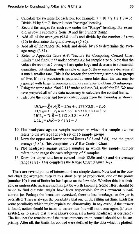
3. Calculate the averages for each row. For example, 7 + 10 + 8 + 2 + 8 = 35.Divide 35 by 5 = 7. Record under "Average" heading.
4. Record the ranges for each row under the "Range" heading. For exam-ple, in row 1 subtract 2 from 10 and list 8 under Range.
5. Add all of the averages (93.8 total) and divide by the number of rows(16) to determine the grand average (5.86).
6. Add all of the ranges (61 total) and divide by 16 to determine the aver-age range (3.81).
7. Refer to Appendix Table A-8, "Factors for Computing Control ChartLimits," and find 0.577 under column A2 for sample size 5. Note that thevalues for samples 2 through 4 are quite large and decrease in substantialquantities; but starting with sample of size 5, these numbers decrease ata much smaller rate. This is the reason for combining samples in groupsof five. If more precision is required at some later date, the test may berepeated with larger groupings and more samples to obtain 30 subgroups.
8. Using the same table, find 2.115 under column D4, and O for D3. We nowhave prepared all of the data necessary to calculate the control limits.
9. Calculate the upper and lower control limits from the formulas as shown.
UCLjc=^+ A2Il = 5.86 + 0.577 X3.81 =8.06LCLx=X-^2R = 5.86 -0.577 X 3.81 = 3.66UCL^= D4^ =2.113 X3.81 = 8.05LCL^= D3R = 0X3.81= O
10. Plot headspace against sample number, in which the sample numberrefers to the average for each set of 16 sample groups.
11. Draw the upper and lower control limits (8.03 and 3.64), and the grandaverage (5.84). This completes the Jf-Bar Control Chart
12. Plot headspace against sample number in which the sample numberrefers to the range for each subgroup of 5 samples.
13. Draw the upper and lower control limits (8.06 and O) and the averagerange (3.81). This completes the Range Chart (Figure 3-8).
There are several points of interest in these simple charts. Note that in the con-trol chart for averages, even in this short burst of production, one of the points(number 10) is out of limits for headspace on the low side. Whether this is a desir-able or undesirable measurement might be worth knowing. Some effort should bemade to find out what might have been responsible for this apparent out-of-control jar. Perhaps the beans are oversized, there is less breakage, or the jar isoverfilled. There is always the possibility that one of the filling machine heads hassome peculiarity which might explain the abnormality. In any event, if the answeris found, action should be taken to assure that this will not occur again (if unde-sirable), or to assure that it will always occur (if a lower headspace is desirable).The fact that the remainder of the measurements are in control should not be sur-prising. After all, the limits for control were defined by the data which is plotted.

Figure 3-8. Range chart.
One conclusion which may be drawn from this initial effort is that the"satisfactory" limits of 3/32 to 4/32, used informally in the past as specifications,are not attainable under this process as it now exists. The current process can runsuccessfully between 3.6/32 and 8/32, and if the tighter specifications are trulyimportant to the quality of the product, considerable work lies ahead to improvethis process.
Having developed this initial control chart, the limits should be used every dayfor a while, plotting headspace averages of five samples taken off the productionline every 30 min. It should not take long to find out if the limits are realistic. Theyshould be refined as more data is gathered, until it can be decided whether processimprovement is needed. Should that point be reached, simple improvements, which
Figure 3-7. X-bar control chart for jelly bean jars.
SAMPLE NUMBER
HEADSPACE
AVERAGE
LCL=O
UCL
HEADSPACE - 5 SAMPLE RANGES
LCLx
AVERAGE
UCLxHEADSPACE
1 POUND JELLY BEAN - Line #3
Headspace in 1/32 inch
SAMPLE NUMBER

management is aware of but has been putting off, should be evaluated and installed.If improvement beyond this is required, a series of experiments should be designedto investigate other means of reaching the specification goals. To measure theeffects of improvements, continue to plot the five sample averages, and if a shift issuspected, prepare a new control chart showing the tighter control limits.
It might be noticed that the range control chart seems to have a downwardtrend. Since all of the values are within the control limits, it is probable that thisunusual pattern has occurred by chance alone. On the other hand, it might beworth an initial investigation to find out if there is some special cause responsi-ble for what appears to be more uniform weight ranges.
The chart for averages (Figure 3-7) shows that the headspace is higher than itshould be for optimum performance; the range chart (Figure 3-8) shows more dis-couraging information. It indicates that even though the average headspace couldbe reduced to a more acceptable level, the range between readings is still going tobe very high. At the moment, the range is plus or minus 4/32, and the presenthoped-for specification limit is very much less at plus or minus 0.5/32. It nowbecomes obvious that there is work to be done to improve the performance of thisline, and that it should probably start by attempting to remove the wide range ofheadspaces currently produced. After that, the target level should also be reduced.
In subsequent chapters on process capacity and process control, there are detaileddiscussions on the meaning and use of quality control charts such as the above.
PROCEDURES FOR CONSTRUCTING ATTRIBUTE CHARTS
There are four commonly used attribute charts, and each has a specific use. Theyare generally easier to construct and to use on a routine basis, though they occa-sionally lack the power of variable charts to spot problem areas quickly. One oftheir major advantages is the simple nature of the concept. They are easilyexplained to line workers and management alike. Most everybody understandsthe meaning of "percent defective" or "number of defects in the lot.** The mathe-matics do not require tables. They can be applied to systems where measurementsconsist of pass-fail and variable measurements are not possible or are difficult toobtain. These are the charts (Table 3-2):
1. p chart with constant lot size: Used to determine control of percent defec-tive units, and to establish whether the process is in control for the day(week, month). "Constant" means "within 20%."
2. p chart with variable lot size: Usually intended to control percent defec-tive units where the number of units varies from sample to sample.Determines if a process is in control for each lot's control limits.
3. np chart (also known as m chart): Used to control the number of defec-tive products in each lot, and to assure that the process is in control.Requires constant lot size.
4. c chart: Used to determine if the number of defects in a single product iswithin control limits. Final inspection.

Table 3-2. Control Charts
SampleLotBased onApplicationGeneral useNameSymbol
Constantandarbitrary
Constant,100% orsample
Varies100%,average orstabilized
Constant
Constant
Varies
Constant
Constant(within20%)
Varies
Constant
Constant orcontinuous
Varies, orone unit
Normaldistribution
Binomialdistribution
Binomialdistribution
Binomialdistribution
Poissondistribution
Poissondistribution
Process control byvariables (inches,ml, pH, ounces, count, etc.)
Process control byattributes: leaks,flavor, blemishes,miscounts, seeds,dents, etc.
Process control byattributes
Process control byattributes
Process control byattributes
Process control byattributes
Locate assignablecause of processshift
Detect processchange
Detect processchange
Detect processchange
Accept orreject item
Accept orreject item
Shewhart
Fraction orpercent defectiveconstant lot
Fraction orpercent defectivevariable lot
Number ofdefectives
Number ofdefectsconstantsample
Number ofdefects,variablesample
XIR
P
P
np
C
U

In Table 3-2 there are three classes of attributes considered: fraction defective(P), number of defectives (np), and number of defects (c, w). The mathematicsinvolved in finding the averages is simply a matter of dividing the total numberof non-acceptables by the number of samples. The calculation for control limitsis based on this figure, and again is an easy calculation. The formulae are shownin Table 3-3.
ExamplesExamples of the three basic types of charts have been selected from different industries toillustrate the broad application of these techniques. The first example is the constructionof a p chart for fraction defective.
Example 1 Percent defectives chart: p chart with constant lot sizeIn a plant producing drums of dill pickle chips, a day's production varies from 476 to 580drums (Table 3-4). Over the years, the major types of defective drums have been found tobe leaks, contamination, discoloration, mislabeled drums, off flavor, overweight andunderweight. In all, there are 18 different types of defects which have been observed. The
Chart name
Examine forNo. of items
in sampleDefectives in lotDefects in lot
P charts
Fraction or% defectiveDefective unitn
np (or /T?)—
np chart
Number ofdefectivesDefective unitn
np (or m)—
c or u chart
Number ofdefectsDefects in unitn (usually 1)
—C
Average fractiondefective
Average defectives
Average defects
Control limits
Table 3-3. Comparison of Attribute Charts
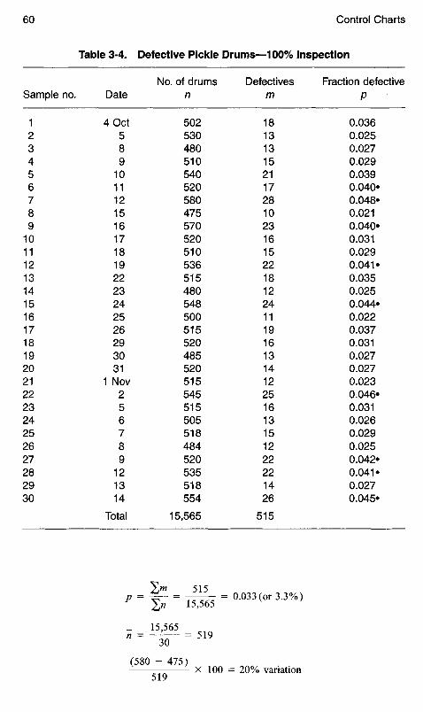
Table 3-4. Defective Pickle Drums— 100% Inspection
Sample no.
123456789
101112131415161718192021222324252627282930
Date
4Oct589
10111215161718192223242526293031
1 Nov256789
121314
Total
No. of drumsn
502530480510540520580475570520510536515480548500515520485520515545515505518484520535518554
15,565
Defectivesm
181313152117281023161522181224111916131412251613151222221426
515
Fraction defectiveP
0.0360.0250.0270.0290.0390.040»0.048«0.0210.040»0.0310.0290.041»0.0350.0250.044»0.0220.0370.0310.0270.0270.0230.046»0.0310.0260.0290.0250.042»0.041»0.0270.045»
variation
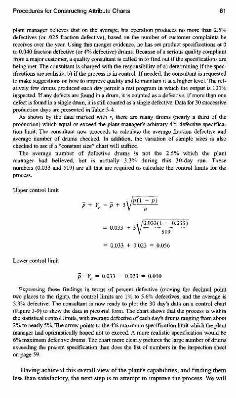
plant manager believes that on the average, his operation produces no more than 2.5%defectives (or .025 fraction defective), based on the number of customer complaints hereceives over the year. Using this meager evidence, he has set product specifications at Oto 0.040 fraction defective (or 4% defective) drums. Because of a serious quality complaintfrom a major customer, a quality consultant is called in to find out if the specifications arebeing met. The consultant is charged with the responsibility of a) determining if the spec-ifications are realistic, b) if the process is in control. If needed, the consultant is requestedto make suggestions on how to improve quality and to maintain it at a higher level. The rel-atively few drums produced each day permit a test program in which the output is 100%inspected. If any defects are found in a drum, it is counted as a defective; if more than onedefect is found in a single drum, it is still counted as a single defective. Data for 30 successiveproduction days are presented in Table 3-4.
As shown by the data marked with •, there are many drums (nearly a third of theproduction) which equal or exceed the plant manager's arbitrary 4% defective specifica-tion limit. The consultant now proceeds to calculate the average fraction defective andaverage number of drums checked. In addition, the variation of sample sizes is alsochecked to see if a "constant size" chart will suffice.
The average number of defective drums is not the 2.5% which the plantmanager had believed, but is actually 3.3% during this 30-day run. Thesenumbers (0.033 and 519) are all that are required to calculate the control limits for theprocess.
Upper control limit
j + r,-; + , <LE5
- 0-033 * 3V0-033<'5,-9°-033)
= 0.033 + 0.023 = 0.056
Lower control limit
p-Yp = 0.033 - 0.023 = 0.010
Expressing these findings in terms of percent defective (moving the decimal pointtwo places to the right), the control limits are 1% to 5.6% defectives, and the average is3.3% defective. The consultant is now ready to plot the 30 day's data on a control chart(Figure 3-9) to show the data in pictorial form. The chart shows that the process is withinthe statistical control limits, with average defective of each day's drums ranging from about2% to nearly 5%. The arrow points to the 4% maximum specification limit which the plantmanager had optimistically hoped not to exceed. A more realistic specification would be6% maximum defective drums. The chart more clearly pictures the large number of drumsexceeding the present specification than does the list of numbers in the inspection sheeton page 59.
Having achieved this overall view of the plant's capabilities, and finding themless than satisfactory, the next step is to attempt to improve the process. We will

LOT NUMBER
Figure 3-9. Fraction defective control chart, constant lot size.
not follow this example to its conclusion, but will indicate the general directionthe consultant will probably take. He will now pinpoint the causes for the defec-tive drums, using a control chart for defects, rather than the broader concept ofdefectives shown in the above chart.
A chart for defects will show some periods where defects are very numerousat or near the upper control limit. The causes should be immediately identified,and new procedures installed to be sure that the problems are not repeated.Conversely, the defect chart also will likely show that on some days the plant iscapable of producing fewer defects than others. By identifying the reasons forthese improvements, additional procedure changes can be installed which willensure that they will be a permanent part of the operation.
Although the processing line is the first place to look for these improvements,there are other areas which may be equally as responsible for defects, and the fol-lowing possibilities should be explored.
• Purchase a better quality of raw materials.• Work with the drum supplier to eliminate substandard drums.• Engineer more gentle handling systems to reduce line damage.• Identify hazardous and critical control points so that national inspection
locations can be installed.• Improve the training of processing personnel.• Revise maintenance schedules so that equipment (scales, slicers, meters,
mixers, thermometers, etc.) will function more reliably.• Study the quality drift cycles to precisely specify sampling schedules.
When the improvements are all in place, and the improvement rate in thedefect chart is leveling off, then it is time to return to the fraction defective
SLICED PICKLE DRUM QUALITYFRACTION DEFECTIVE CONTROL CHART FOR AVERAGES
FRACTIONDEFECTIVE
UCL
AVG
LCL
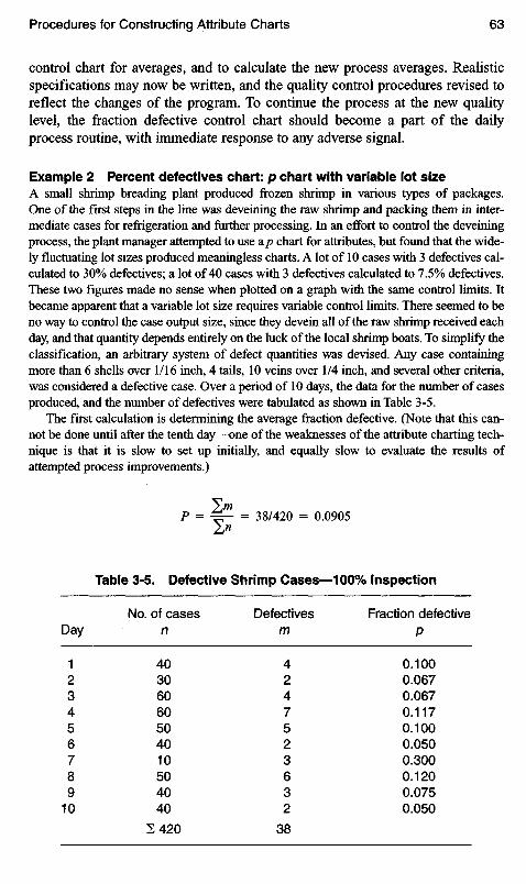
control chart for averages, and to calculate the new process averages. Realisticspecifications may now be written, and the quality control procedures revised toreflect the changes of the program. To continue the process at the new qualitylevel, the fraction defective control chart should become a part of the dailyprocess routine, with immediate response to any adverse signal.
Example 2 Percent defectives chart: p chart with variable lot sizeA small shrimp breading plant produced frozen shrimp in various types of packages.One of the first steps in the line was deveining the raw shrimp and packing them in inter-mediate cases for refrigeration and further processing. In an effort to control the deveiningprocess, the plant manager attempted to use ap chart for attributes, but found that the wide-ly fluctuating lot sizes produced meaningless charts. A lot of 10 cases with 3 defectives cal-culated to 30% defectives; a lot of 40 cases with 3 defectives calculated to 7.5% defectives.These two figures made no sense when plotted on a graph with the same control limits. Itbecame apparent that a variable lot size requires variable control limits. There seemed to beno way to control the case output size, since they devein all of the raw shrimp received eachday, and that quantity depends entirely on the luck of the local shrimp boats. To simplify theclassification, an arbitrary system of defect quantities was devised. Any case containingmore than 6 shells over 1/16 inch, 4 tails, 10 veins over 1/4 inch, and several other criteria,was considered a defective case. Over a period of 10 days, the data for the number of casesproduced, and the number of defectives were tabulated as shown in Table 3-5.
The first calculation is determining the average fraction defective. (Note that this can-not be done until after the tenth day—one of the weaknesses of the attribute charting tech-nique is that it is slow to set up initially, and equally slow to evaluate the results ofattempted process improvements.)
Day
123456789
10
No. of casesn
40306060504010504040
E 420
Defectivesm
4247523632
38
Fraction defectiveP
0.1000.0670.0670.1170.1000.0500.3000.1200.0750.050
Table 3-5. Defective Shrimp Cases—100% Inspection

The upper control limit for the fraction defective is defined as:
\ /P(I -p)C L Y p = p ± 3y/^r^-
= 0.0905 + 3 V {0.0905(1 - 0.0905)}/«
= 0.0905 + 3V0.0824«
Since n varies for each day, the calculation for the upper control limit isperformed each day, using this formula. The results are shown in Table 3-6 under thecolumn, Control Limit UCL.
Plotting the fraction defectives for each day is performed in the same way as for aconstant lot size (see Figure 3-9). The difference arises when the control limits are plotted.The lower limit is so close to zero that a lower control limit would not be particularly useful.
The upper control limits are plotted for each sample size. Thus, the sample size for day1 is n = 40. The corresponding upper control limit is 0.227. Continuing, the control limitsfor each day are plotted along with that day's fraction defective until all 10 points arecompleted.
Interpreting the chart in Figure 3-10 discloses that for the relatively small sample sizes forthe shrimp example, the control limits are very liberal, and suggest that the quality level wouldhave to be atrocious before a day's production is out of limits. As a matter of fact, the frac-tion defective average of 0.0905 (or 9%) is already an index of very poor quality perform-ance, and yet even at this level, the operation appears to be in statistical control. As was thecase with other control charts, when the sample size increases, the upper control limitchanges less and less. This is clearly shown by comparing the distance on the vertical axisbetween n = 10 and n - 20, with the distance between n = 50 and n = 60. Most of the dayssampled exhibited defective levels clustered near the 0.0905 average except for the spike dataof Day #7. Again, even though this day showed a distressing level of 30% defectives, thenumbers involved (3 out of 10 cases) are so small as to allow the control limits to indicate
Table 3-6. Defective Shrimp Cases—100% Inspection: Calculation ofControl Limits
Day
123456789
10
No. of casesn
40306060504010504040
Defectivesm
4247523632
Fraction defectiveP
0.1000.0670.0670.1170.1000.0500.3000.1200.0750.050
Control limitUCL
0.2270.2480.2020.2020.2120.2270.3630.2120.2270.227
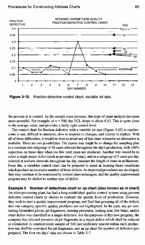
Figure 3-10. Fraction defective control chart, variable lot size.
the process is in control. As the sample sizes increase, this type of chart analysis becomesmore powerful. For example, at n = 500, the UCL drops to about 0.13. This is quite closeto the average value, and provides a fairly tight control level.
The control chart for fraction defective with a variable lot size (Figure 3-10) is cumber-some to use, difficult to interpret, slow to respond to changes, and clumsy to explain. Withall of these difficulties, it would be wise to avoid use of this chart whenever an alternative isavailable. There are two possibilities. The easiest way might be to change the sampling planto a constant size subgroup of 30 cases selected throughout the day's production, with 100%inspection on those days when too few total cases are produced. Another way would be toselect a single major defect (such as presence of veins), and in a subgroup of 5 cases per day,selected at uniform intervals throughout the day, measure the length of veins in millimeters.From this, a variables control chart can be prepared to assist in locating those conditionswhich produce an excessive number of these defects. As improved procedures are developed,they may continue to be monitored by control chart techniques, and the quality improvementprogram may be shifted to another type of defect.
Example 3 Number of defectives chart or np chart (also known as m chart)An olive processing plant has had a long-established quality control system using percentdefective control charts (p charts) to evaluate the quality level of production. However,they wish to start a quality improvement program, and find that grouping all of the defectsinto one category, specific quality problems are not highlighted. In the past, any jar con-taining blemished pieces, pit fragments, missing pimientos, leaking seal, low brine, and/orother defect was classified as a single defective. For the purposes of this new program, thecompany has selected presence of pit fragments as a major defect which shall be reducedor eliminated. A constant-sized sample of 500 jars uniformly spaced within each produc-tion run shall be examined for pit fragments, and an np chart for number of defective jarsprepared. The first ten days' data are shown in Table 3-7.
DAY NUMBER
FRACTIONDEFECTIVE
DEVEINED SHRIMP CASE QUALITYFRACTION DEFECTIVE CONTROL CHART
AVERAGE
UCL

The calculations based on the data establish the average number of defectives, theaverage fraction defective, and the control limits.
Average number of defectives
=-£-f--"Average fraction defective
— - - mm = np p = —
n
= 12.9/500 = 0.026
Control limits
CL = m ± 3Vm(I - p)
= 12.9 ± 3Vl2.9(l - 0.026)
= 12.9 ± 10.6
A control chart may now be constructed using these figures:Average number of defectives =12.9Upper control limit = 12.9 + 10.6 = 23.5Lower control limit = 12.9 - 10.6 = 2.3
Figure 3-11 provides a good starting point to improve the quality of theproduct insofar as pits are concerned. It shows that the pit level centers around12.9%, and that the quality level stays fairly close to that level. On day 7, someabnormality in the process caused the defects to rise out of limits on the high side,
Day
123456789
10
N=W
Sample size(n)
500500500500500500500500500500
En = 5000
Number of defectives(m) or np
14141710138
24118
10
Zm= 129
Table 3-7. Data for Defective Olive Jars

and operating conditions for that day should be examined closely for clues. Thosefamiliar with the industry would know the most likely places to look—a changein raw material, maintenance programs on the pitter equipment, line speeds, andnew line workers. If the "special cause" for this unusual day's production can befound, steps should be taken to insure that it cannot happen again. After a fewmore days of production with this process modification, a new chart should beprepared with its associated closer control limits. Any time a point falls outsideof limits, it should be analyzed to improve the process. At the same time, anyobservation which drops below the lower control limit should be studied withequal care, since it too may point to directions for quality improvement.
To see the effect of eliminating the problem responsible for the out-of-controllevel of day #7, replace the 24 with 12.9, and calculate a new set of control points.The average would be reduced slightly to 11.8, and the upper control limit wouldnow be 22.0. The significance of this little exercise is that it demonstrates howremoval of just this one special cause of product quality variation can reduce theaverage defects by about 1%, and reduce the upper control limit by 1.5%. It shouldbe obvious that continuing with this quality control chart, and eliminating otherspecial causes as they are discovered will appreciably reduce the defects caused by thepresence of pits. Once the procedure reaches an equilibrium, and further improvementappears unlikely, the next most important defect (perhaps blemishes) may be exploredin a similar manner. An impatient manager might find this process painfully slow, butit can be a very effective quality improvement procedure to follow.
Example 4 Number of defects chart: constant size sample c chartIn contrast to all of the above charts where the quality issue is the number of defectives,the c chart is concerned only with the number of defects. The number of defects is
DAY NUMBER
Figure 3-11. Number of defectives (np) control chart.
AVERAGE
LCL
UCL
NUMBER OFDEFECTS
OLIVE JAR PIT DEFECTIVESnp CHART FOR NUMBER OF DEFECTS

measured for a subgroup of fixed size, and very often is concerned with a sample of size1. The process to be measured may be a continuous one in which samples of a standard-ized number of units are selected at a prescribed constant interval. Or a process producinga constant lot size may be checked with a standardized sample size. The sample of size 1refers to a process in which the end product is a single sample: a batch of corn syrup, aside of beef, a vat of chocolate, a bin of blended tea.
For our example, we shall select a batch of flavored syrup produced by a bottler of car-bonated fruit drink. Ordinarily, a single batch of fruit-flavored syrup is produced each dayto be diluted and packed on the following shift. The defects commonly found during qual-ity control evaluations are: foreign matter, temperature above 490F, poor color, pH over 5.3,weak flavor, concentration incorrect (for each of 22 ingredients), incorrect viscosity,excessive bacteria (6 tests), yeast, or molds. The following data (Table 3-8) was obtainedover ten production days.
Again, we find one of the batches out of control in the initial chart. With thelarge number of attributes entered into the data, it is apparent that at least one ofthem is seriously out of control. If possible, the factor responsible should be iso-lated and studied under its own control chart until a reason for the variation hasbeen isolated. At that point, new procedures should be initiated to prevent furtheroccurrence of this defect in a day's batch. If the identity of the cause defectcannot be easily determined, control charts for small groups of defects should beprepared until the problem is uncovered.
Table 3-8. Data for Syrup Batch Defects
Sample number
123456789
10
Date
Feb. 345671011121314
Number of defects (c)
15212718391018221318
Ec= 201

Example 5 Number of defects chart: variable size sample u chartThe u chart is a special case of the c chart, and has limited use in the food processingindustry. It is applied to products where the number of units in the sample subgroup vary—and they may vary from a subgroup of 1 to perhaps a dozen units. The defects are fed intoan equation to reduce the data to the number of nonconformities in a subgroup. The con-trol limits are calculated in the same manner as for the c chart, except that the control lim-its are divided by the square root of the number of units in the subgroup. At best, this typeof control chart serves as a score card to let management know how the quality was forsome past period of time. It is slow to react to quality control problems, and it is recom-mended that other types of control charts be used before considering the u chart. Even inthe automotive manufacturing industry where the u chart is used in an attempt to controlthe number of defects in fenders or bumpers, it has limited effectiveness. It might be usedas a blunt weapon to brandish at parts suppliers in an effort to assist them in productimprovement, but it carries few if any suggested cures. With this bleak description and thelimitations of the u chart, no example will be presented here.
It is difficult to generalize on the use and effectiveness of attribute charts of alltypes since there are so many possible applications in so many different food pro-cessing industries. Generally speaking, they are slow to react, and tend to be con-structed in such a way as to include a number of quality problems under oneformat. They do provide management with an easily understood picture of howthe quality has been controlled over some period of time. There are, of course,some applications where precise variable measurements of a process are neitherpossible nor desirable, and attribute charts are satisfactory. Under some circum-stances they can suggest areas where the process should be modified to bettercontrol the quality level, or in some instances, to actually improve the qualitylevel. The one generalization which might be made is: wherever possible, select avariable control chart instead of an attribute chart to control process quality.
This chapter has not covered all of the charts which are available for use inquality control applications. Many of them have specialized uses for specialindustrial applications. Many are complicated, and are perhaps best understood bythe statisticians who have created them than by the plant operating and qualitycontrol personnel who must use them. Some mature industries tend to take shortcuts with the classical chart techniques discussed above. This is somewhat risky.An example is the abandonment of range charts when experience has shown thatthe averages chart is sufficiently indicative of process quality. Sooner or later, onewould expect to miss an out-of-control period of production when, for example,a worn machine abruptly spews out widely varying product which somehow con-tinues to average out within the control limits. This is not to suggest that someexperimentation with the tried and true control chart technique should not beattempted. But it is strongly recommended that experimentation be delayed untilafter all plant processes have been exposed to the simpler procedures long enoughto ensure that all the processes are under excellent control, and that further qual-ity improvements using these principles are unlikely to be uncovered.

4 Fundamentals
There are four distributions of data which form the basis for statistical qualitycontrol: Binomial, Poisson, Normal and Student's t. Common to these distributionsare the concepts of measures of central tendency and measures of dispersion.
ANALYSIS OF DATA
Measures of Central Tendency
In order to illustrate a large quantity of data (population) with a single number,perhaps the best single measure is the arithmetic mean. This is simply the total ofall values, divided by the number of items.
X1 + X2 + X3 + -•- + Y YMean(M)= J \ I *L = y±^ N 2^N
Another illustration of the data is called the Median. When the numbers arearranged in order of magnitude, the Median of the set of data is the middle numberif N is odd, and the average of the two middle numbers if N is even. For example:
2,3,7,9,21,22,45,67,68,69,72
Median = 22
4, 6, 9, 12, 24, 45, 56, 58, 59, 63, 68, 69
Median = (45 + 56)12 = 50.5
As can be seen from these illustrations, neither the mean nor the median hasto be one of the numbers observed in the set of data.

Table 4-1 . Database, Set A: Net Weights, 1 84-g Jars of Pistachios
Sample
1234567891011121314151617181920
X1
187186187190188187194183189188187188186189190188185187194186
X2
190182189189188185189188192186187188189184186189188187183188
X3
183183192189183187194187194193188190194194189185193190191188
X4
185185192187187190186187183191182190186188191185188189191180
X5
188189188187183185187183188185183183192190187183188183192186
Total
933925948942929934950928946943927939947945943930942936951928
Mean
186.6185189.6188.4185.8186.8190185.6189.2188.6185.4187.8189.4189188.6186186.4187.2190.2185.6
EX- 18,766 X = 18,765
Tables 4-1 and 4-2 demonstrate calculation of the population mean by differentmethods. Both examples are based on the same data obtained by weighing the netcontents of 184-g jars of pistachios taken in sequence from the production line.The data has been arbitrarily arranged in groups of five weighings. The firstmethod for calculating the mean is based on the actual data; the second methoduses deviations from the target weight of 184 g. Both produce the same mean. Themean of the population is known as /jt; the mean of the samples representing thepopulation is X.
Measures of Dispersion
The mean and the median do not provide much information about the distributionof the data. Two different sets of data may have the same means, but the disper-sion of the data about the two means may be totally different. The dispersionis better described by three other expressions: Range, Variance, and StandardDeviation.
The Range (R) is found simply by subtracting the smallest value from thelargest value found in the data. By itself, the range has limited use. This is because

Table 4-2. Deviations from 184-g (X- 184). Jars of Pistachios
Sample
123456789
1011121314151617181920
Xi
323643
10-1
5434256413
102
X2
6-2
55415482345O2543
-14
X3
-1-1
85
-13
103
10946
1010519674
X4
11833623H
7-2
62471457
-4
X5
4543
-113
-141
-1-1
863
-14
-182
Total
135
28229
14308
26237
19272523102216318
366
Mean
2.615.64.41.82.861.65.24.61.43.85.454.624.43.26.21.6
73.2
Range
77535585
118678
105687
118
140
Note: X= 184 + (366/100) - 187.66.
the smallest or the largest value may be extremely far from the mean value, thusgiving an exaggerated impression of the dispersion of data.
For this reason, the Variance a2 is more commonly used to measure dispersionof data. The variance is calculated by subtracting each item (X) in the distributionfrom the mean /JL, squaring each of the resulting figures, adding the results, anddividing by the number of items (N). Note that if the subtraction operation werenot squared, the final figure would be zero, since half of the values are positiveand half of the values are negative with respect to the mean. Another way toexpress this: the average of all of the deviations from the mean will always turnout to be zero. By squaring, all of the figures become positive.
Unfortunately, the Variance is expressed as the square of some number, andhas limited direct use in quality control. For example, if all of the observationswere weights of a distribution of packages, the variance calculated as abovewould be expressed in (grams)2. To eliminate this complication, the square rootof the variance is commonly determined, and the resulting figure is referred toas the Standard Deviation or a. When using this formula to determine Varianceand Standard Deviation, there are many opportunities for calculation errors
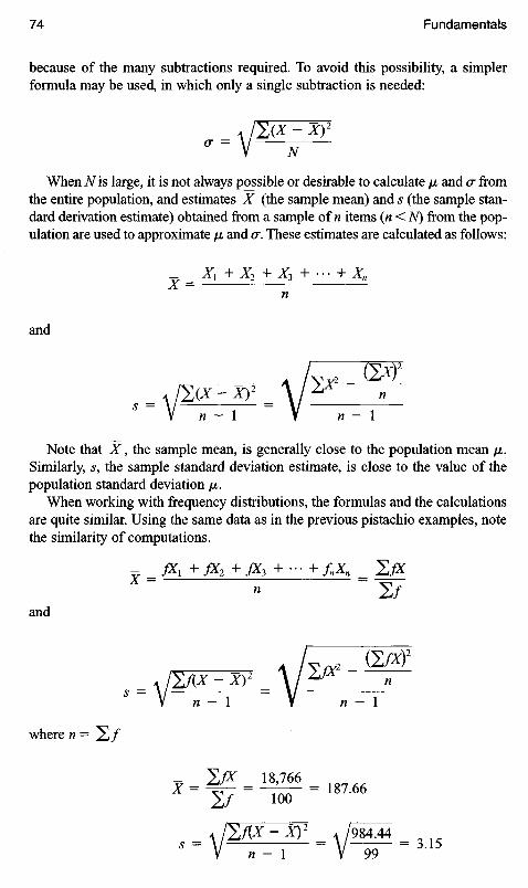
because of the many subtractions required. To avoid this possibility, a simplerformula may be used, in which only a single subtraction is needed:
A JI1(X ~ y>2"^ = V N
When N is large, it is not always possible or desirable to calculate /^ and or fromthe entire population, and estimates X (the sample mean) and s (the sample stan-dard derivation estimate) obtained from a sample of n items (n<N) from the pop-ulation are used to approximate /JL and cr. These estimates are calculated as follows:
^_X, +X2 +X, +"- + XnJ\. —n
and
, /^TWv/№-*)2 A / — n—
S = M n - l = V n - l
Note that X, the sample mean, is generally close to the population mean /i.Similarly, s, the sample standard deviation estimate, is close to the value of thepopulation standard deviation JJL.
When working with frequency distributions, the formulas and the calculationsare quite similar. Using the same data as in the previous pistachio examples, notethe similarity of computations.
and
where

Figure 4-1. Histogram for distribution of weights.
The "Frequency" columns in Table 4-3 are more usually assembled verticallyin a format referred to as a histogram. The same data have been rearranged asshown in Figure 4-1 and Table 4-4.
* = 184 + T^ = 187'66IUU
Weight in Grams
Frequency
Range of weights = 194-180.
Table 4-3. Frequency and Standard Deviation Calculations for Pistachios
X Frequency f fX X-X f(X - X)2
180181182183184185186187188189190191192193194
1O21218S15171184526
100
180O
36421961841480148828053196207915207649603861164
18766
-7.66-6.66-5.66-4.66-3.66-2.66-1.66-0.660.341.342.343.344.345.346.34
58.6756O64.0712260.587213.3956,56.604822.04486.53401 .965219.751643.804844.622494.178057.0312241.1736
984.44

Table 4-4. Range of Differences = (X-184)
X-184 f fX fX2
-4 1 -4 16- 6 0 0 0- 2 2 - 4 8-1 12 -12 120 1 O O1 8 8 82 8 16 323 15 45 1354 17 68 2725 11 55 2756 8 48 2867 4 28 1968 5 40 3209 2 18 16210 6 60 600
100 366 2324
PROBABILITY
Statistics and probability are so fundamentally interrelated that it is impossibleto discuss statistics without an understanding of the meaning of probability.Probability theory makes it possible to interpret statistical results. Many of thestatistical procedures involve conclusions which are based on samples, and theseare always affected by random variation. Probability theory allows us to expressnumerically the inevitable uncertainties in drawing these conclusions.
When assessing the quality of a lpt of goods, rarely is the total lot examinedpiece by piece. The costs associated with such a practice generally make it imprac-tical, and it has been shown that 100% inspection is rarely 100% effective becauseof inaccuracies. These may be caused by limits of the test procedures, or boredomof the inspectors, often leading to near hypnosis which allows defects to pass unno-ticed. Instead, a sample of the lot is usually tested, and the number of defective arti-cles recorded. In order for this result to be meaningful, the sample should berepresentative of the lot, and selected in such a way that each article within the lothas an equal chance of being selected. This is referred to as a random sample.
Within a lot, if there are r defective articles in a random sample of n articles,then, in the selection of each article from the lot, the probability of obtaininga defective article is p = r/n, and the probability of obtaining a nondefectivearticle is q = (n — r)ln. In the event that /7 = 0, there are no defective articles;should p = 1, all articles are defective.
For example, if 1/10 (or 10%) of the articles in a lot are defective, then 9/10(or 90%) are nondefective. This may also be expressed as/? = 1/10, and q = 9/10.
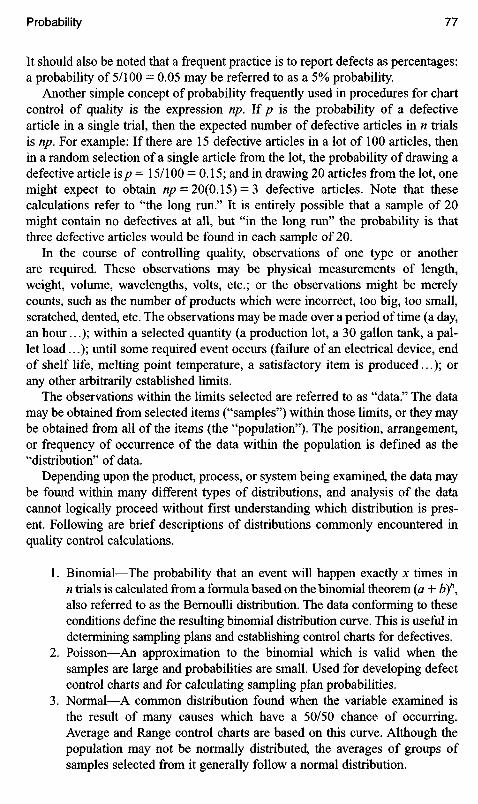
It should also be noted that a frequent practice is to report defects as percentages:a probability of 5/100 = 0.05 may be referred to as a 5% probability.
Another simple concept of probability frequently used in procedures for chartcontrol of quality is the expression np. If p is the probability of a defectivearticle in a single trial, then the expected number of defective articles in n trialsis np. For example: If there are 15 defective articles in a lot of 100 articles, thenin a random selection of a single article from the lot, the probability of drawing adefective article is p = 15/100 = 0.15; and in drawing 20 articles from the lot, onemight expect to obtain np = 20(0.15) = 3 defective articles. Note that thesecalculations refer to "the long run." It is entirely possible that a sample of 20might contain no defectives at all, but "in the long run" the probability is thatthree defective articles would be found in each sample of 20.
In the course of controlling quality, observations of one type or anotherare required. These observations may be physical measurements of length,weight, volume, wavelengths, volts, etc.; or the observations might be merelycounts, such as the number of products which were incorrect, too big, too small,scratched, dented, etc. The observations may be made over a period of time (a day,an hour...); within a selected quantity (a production lot, a 30 gallon tank, a pal-let load...); until some required event occurs (failure of an electrical device, endof shelf life, melting point temperature, a satisfactory item is produced...); orany other arbitrarily established limits.
The observations within the limits selected are referred to as "data." The datamay be obtained from selected items ("samples") within those limits, or they maybe obtained from all of the items (the "population"). The position, arrangement,or frequency of occurrence of the data within the population is defined as the"distribution" of data.
Depending upon the product, process, or system being examined, the data maybe found within many different types of distributions, and analysis of the datacannot logically proceed without first understanding which distribution is pres-ent. Following are brief descriptions of distributions commonly encountered inquality control calculations.
1. Binomial—The probability that an event will happen exactly x times inn trials is calculated from a formula based on the binomial theorem (a 4- b)n,also referred to as the Bernoulli distribution. The data conforming to theseconditions define the resulting binomial distribution curve. This is useful indetermining sampling plans and establishing control charts for defectives.
2. Poisson—An approximation to the binomial which is valid when thesamples are large and probabilities are small. Used for developing defectcontrol charts and for calculating sampling plan probabilities.
3. Normal—A common distribution found when the variable examined isthe result of many causes which have a 50/50 chance of occurring.Average and Range control charts are based on this curve. Although thepopulation may not be normally distributed, the averages of groups ofsamples selected from it generally follow a normal distribution.

4. ^-Distribution—A somewhat nonnormal curve produced when comparingsamples and population means when the population standard deviationsare unknown and must be estimated from the samples.
5. F-Distribution—The distribution of the ratio of two estimates of variance.6. Exponential—Logarithmic curves which describe events such as flavor
loss, shelf life, or container failure.7. Weibull—These may take many shapes, and are based on a single
formula with three variables: shape, scale, and location. Used to studyshelf life and product failure rates.
8. Chi-Square—As contrasted with ^-distribution, the chi-square distributionis used when the standard deviations are known for the sample and for thepopulation. These are then compared.
9. Others—Multinomial (a generalization of the binomial), hypergeometric(samples removed from population for testing are not replaced), uniform,Cauchy, gamma, beta, bivariate, normal, geometric, Pascal's, Maxwell.
BINOMIAL DISTRIBUTION
Many quality control problems deal with a population in which a proportion^ ofthe individuals have a certain characteristic, and a proportion q = 1 —p of theindividuals do not. This is called a binomial population since each individual in itfalls into one of only two classes. Sampling for defective articles in a lot whereeach article selected at random is either good or defective leads to a binomialdistribution.
In a random selection of a sample size n from a large lot, ifp is the probabilityof obtaining a defective item in each draw, and q = 1 —p is the probability ofobtaining a nondefective item, then the probability P(r) that there will be exactlyr defective items in the sample size n is the term in the binomial expansion of(q +p)n for which the exponent ofp is r; that is:
P(r) = (nr}qn~rpr
where
(*) = »*(r> (n-r)lrl
(Value of (^) may be found in Table A4 in the Appendix.)
A distribution whose terms are proportional to successive terms of the binomialexpansion is called a binomial distribution. Its mean is JJL = np, and its standard
deviation: a — \/npq
A binomial probability distribution may be represented by a histogram. This is afigure obtained by plotting all possible values of r along a base line, and erectingon each an equal-base rectangle whose height (and area) is proportional to thecorresponding probability.
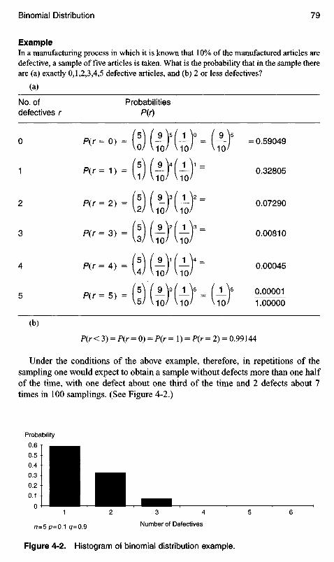
Under the conditions of the above example, therefore, in repetitions of thesampling one would expect to obtain a sample without defects more than one halfof the time, with one defect about one third of the time and 2 defects about 7times in 100 samplings. (See Figure 4-2.)
ExampleIn a manufacturing process in which it is known that 10% of the manufactured articles aredefective, a sample of five articles is taken. What is the probability that in the sample thereare (a) exactly 0,1,2,3,4,5 defective articles, and (b) 2 or less defectives?
(a)
(b)
Probability
Number of Defectives
Figure 4-2. Histogram of binomial distribution example.
No. ofdefectives r
ProbabilitiesP(i)
O
1
2
3
4
5
0.59049
0.32805
0.07290
0.00810
0.00045
0.000011.00000
n=5p=0.1 c/=0.9

Figure 4-3. Histogram for p = q - 0.5.
In the event that the values of p and q approach equality (for example:P = q = 0.5), the histogram for any value of n approaches symmetry around thevertical line erected at the mean. The total area included in the blocks of the his-togram always equals 1. (See Figure 4-3.)
Poisson Distribution
An approximation to the binomial distribution, the Poisson distribution, may beused when:
1. the probability of defectives is small (less than 0.1%);2. the number of observations is large (more than 16);3. the sample is small compared to the population (<10%).
The Poisson distribution may be used to prepare control charts for defects,but perhaps has its greatest use in calculating probabilities for developingsampling plans. Much of the mathematics has been prepared in the form of atable which simplifies its use. (See Table A-I in the Appendix.) This tablegives the sums of the probabilities of c or fewer defects for various values ofnp'=cf.
lfn is large and/? and q are small so that np is fairly small, that is:
Ou - np < 5)
then the binomial probability:
p(r) = (?)«"-y
is given approximately by the equation:
(npYP(r = c) = e~np^- (r = c = 0,l,2,...,n) and e = 2.178...
No. of defectives
Pro
b.

A distribution where the frequencies are given by this formula is called aPoisson distribution, and is extremely useful in the inspection and control ofmanufactured goods where the proportion of defective articles/?' in a large lot isexpected to be small. Following are several examples:
Example 1In a large shipment of articles 5% are known defective. What is the probability that in asample of 100 articles from the shipment, there are 2 or fewer defectives?
/Lt = /ip"=100(.05) = 5; c = 2
\c No. of defectivesnp'\ 0 1 2 3 4 5 6 7 8(Mean 5.0) 0.007 0.040 0.125 0.265 0.440 0.616 0.762 0.867 0.932
(From Table A-I.)
Therefore: p(c = 2) = 0.125 is the probability of 2 or fewer defectives. That is, the chancesare between 12 and 13% that a sample of 100 will contain 2 or fewer defectives.
Example 2If the true process average of defectives (proportion defective) is known to be 0.01, findthe probability that in a sample of 100 articles there are (a) no defectives, (b) exactlytwo defectives, (c) fewer than 5 defectives, (d) at least 5 defectives (i.e., 5 or more).Here, JJL — np1 — 100(0.01)= 1; c = number of defectives less than and including c. (Itnormally is the acceptance number; i.e., the maximum allowable number of defectsin a sample of size n to be acceptable.) We shall use the table to find probabilities forvarious values of c.
(a) P(c = O) = 0.368(b) P[(c = 2)-(c= I)] = 0.920-0.736 = 0.184(c) P(c = 4) = 0.996(d) P[I - (c = 4)] = 1 - 0.996 = 0.004 (total of all terms = 1)
Example 3A pump in a cannery has a failure, on the average, once in every 5000 hours of operation.What is the probability that (a) more than one failure will occur in a 1000-hour period,(b) no failure will occur in 10,000 hours of operation?
(a) np' = 1000(1/5000) = 1/5 = 0.20. Since the table gives the probability of one orless failures at c = 1, then the probability of more than one failure is represented byP[I — (c — I)] since the total of all terms = 1. From the table,
P[I - (c = I)] = 1 - 0.982 = 0.018
(b) np' = 10,000(1/5000) = 2; c = O.
From the table, P(c = O) = 0.135.

Example 4A purchaser will accept a large shipment of articles if, in a sample of 1,000 articles takenat random from the shipment, there are at most 10 defective articles. If the entire shipmentis 0.5% defective, what is the probability that the shipment will be accepted?
/i/>'= 1000(0.005) = 5; c=10
From the table, P(C= 10) = 0.986. Therefore, the shipment has a 98.6% probability ofbeing accepted.
THE NORMAL DISTRIBUTION
In quality control, the normal distribution has the widest application of any of thedistributions. In the binomial and Poisson distributions, the random variable takesonly a countable (or discrete) number of possible values. By contrast, there aremany observations which involve a process of measurement, and in all suchprocesses we are dealing with quantities which have an infinite number of grada-tions. This gives rise to the normal distribution; as the number of gradations (n)approaches infinity, the histogram resulting approaches a curve (see Figures 4-4and 4-5). Early studies of the weights of groups of people, or lengths of cornstalks, or other naturally occurring phenomena produced distributions whichapproximated a bell-shaped curve. Because this curve is found so often in nature,it was assigned the name "Normal Curve."
A clingstone peach cannery may have a target drained weight of 19 ounces ina 2 Y size can. If the filling operation is in control, most of the production will cen-ter near the target weight, but the frequency will taper off from the average as the
Figure 4-4. Normal distribution as n increases.
n=2 n=3 n=4 n=6 n=10 n=28

deviations become wider. The need to establish attainable control weight limits oneither side of the target weight is obvious, since the consumer feels cheated if theproduct weighs less than stated (and this could be in violation of the law), andoverly excessive weights can be costly to the producer. The normal distribution isused to calculate the values of "less than stated" and "overly excessive weights."
The equation which defines the normal probability is:
where P is the relative frequency (or probability) with which a value of Xoccurs and where /x and a are the mean and standard deviation, respectively(TT = 3.1459 and e = 2.178). The value of cr determines the concentration of dataabout the mean, as shown in Figure 4-5.
In order to understand the power of the normal curve and its application toquality control, let us consider some of its universal qualities. The areas under thenormal curve represent probabilities of the normal distribution. As was the caseof the histograms depicting the binomial distribution, the total area under thenormal curve equals 1. Therefore, areas under the curve may be considered asproportions, probabilities, and (when multiplied by 100) as percents.
In the Figure 4-6, the area A under the normal curve between two vertical linesat X1 and X2 represents the probability that a randomly drawn measurement X willfall betweenX1 andX2. In algebraic terms: P(X1 >X>X2)=A.
To simplify calculations, it is customary to use tables to find the areas underthe normal curve. Since there is an unlimited number of normal curves, the tableswere constructed for universal use as follows: the deviation of any measurementX from the mean is expressed in terms of standard deviations, that is,
Referring to Figure 4-6,
Figure 4-5. Frequency distributions with differento- values.

Figure 4-7. Areas under the normal curve,
and
Table A-2 in the Appendix is a compilation of areas under the normal curve tothe right of valves of Z (or to the left of valves of — Z). Certain special areas areshown in Figure 4-7. These areas are designated by horizontal axis divisionsexpressed in the terms of the two scales: X- /JL and Z.
DISTRIBUTION OF SAMPLE MEANS
Many references are made to "parameters" and "statistics" when discussing nor-mal distributions. The following definitions should make these differences clear:
Parameters—these are the values of JJL (the mean) and a (the standarddeviation) obtained from the population.
Figure 4-6. Area of probability between X1 and X2.

Statistics—these are the values of X and s, the estimates of JUL (the mean) andcr (the standard deviation) obtained from samples.
The relation between the population and samples taken from that populationis of vital importance to establishment of quality control chart methods. Thatrelationship is:
1. If measurements in a population are distributed normally, then averages ofgroups of measurements from that population will be found to be closerto the mean than the original measurements.
2. (and this is even more vital) If measurements of a population are NOTdistributed normally, averages of groups of measurements from thatpopulation WILL approach a normal distribution.
This may be expressed in mathematical terms. When a lot or population issampled, the sample mean is usually denoted as X. Sampling generates a popu-lation of X's with a mean /% and standard deviation aj of its own. If thepopulation consists of k sample means, X, it can be shown that:
I^ \ fc(X ~ M)2 a-^ = T = * ^ = V * =Vn
To state this in words: if a set of measurements X has a distribution withmean JJL and a standard deviation a, and if all possible samples of n measurementsare drawn, then the sample mean X will have a distribution which, for larger andlarger n, approaches the normal distribution with mean JJL and standard deviationcr/Vn This is known as the Central Limit Theorem, and states that for signifi-cantly large n (at least 30), X will be approximately normally distributed, even ifthe original population of Xs does not satisfy a normal distribution.
Figure 4-8 demonstrates the way in which the population distribution isnarrowed as the sample size is increased from 4 to 16 measurements. Threecurves are shown: the distribution of the population from which the samples aredrawn; the distribution of sample means when samples of size 4 are selected; andthe distribution of sample means when samples of size 16 are selected. Withincreasing n, the curve becomes taller and narrower. The areas under the curveswill always be equal to one. Probabilities for X values can be found from TableA-2 in the Appendix by calculating
z^X~ fJL = X~ ft
<?x 0-lVn
where a/Vn is the standard deviation of the means and (TX is thestandard deviation of a sample of n items.

Figure 4-8. Comparison of population curve with curves fortwo sample sizes.
Example 1If the drained weights of canned peaches follow a normal distribution with JJL= 19.0ounces and a standard deviation of cr = 0.2 ounce, what is the probability of a can select-ed at random having a drained weight (a) between 19.1 and 19.2 ounces; (b) between 18.7and 19.1 ounces; and (c) less than 18.8 ounces?
(a) X1 = 19.1; Z1 = * = — = 0.5; A1 (from Table A-2) = 0.3085
19.2 - 190 02X2 = 19.2; Z2 = = — = 1.0; A2 (from Table A-2) = 0.1587
P(19.2<X< 19.2) = AI -A2 = 0.3085 - 0.1587 = 0.1498
Therefore, about 15% of the drained weights are between 19.1 and 19.2 ounces. (SeeFigure 4-9a.)
107 190 03(b) X1 = 18.7; Z1 - —— = — - - 1.5; A1 (from Table A-2) = 0.0668
X2 = 19.1; Z2 = 19-1 ~ 19'° = — = 0.5 (from Table A-2) = 0.3085
P(18.7 <X< 19.1) = 1 - (A1 +A2) = 1 - 0.3753 = 0.6247
Therefore, about 62.5% of the drained weights are between 18.7 and 19.1 ounces. SeeFigure 4-9b.
1 0 0 19 O(c) X = 18.8; Z = — = -1.0; A = 0.1587
P(X< 18.8) =,4 = 0.1587
Therefore, between 15% and 16% of the cans have contents the drained weights ofwhich are less than 18.8 ounces. See Figure 4.9c.

Figure 4-10. Distribution chart, showing medium grade areafor Example 2.
Example 2In a packing plant grading Satsuma plums whose weights are normally distributed, 20%are called small, 55% medium, 15% large, and 10% very large. If the mean weight of allSatsuma plums is 4.83 ounces with a standard deviation of 1.20 ounces, what are the lowerand upper bounds for the weight of Satsuma plums graded as medium?
Since = 0.20, from Table A-2 the corresponding value of Z1 is —0.84, and forA2 = 0.25 the nearest value of Z2 from the table is 0.67. Then
X1 - 4.83 X2 ~ 4.83z-- -°-84 = -T20-7^ =0-67 = -r*r-Then, solving for X\ and X2 we get
X1 = 4.83 - (0.84)(1.20) X2 = 4.83 + (0.67)(1.20)= 4.83-1.01 =4.83 + 0.80= 3.82 ounces =5.63 ounces
Therefore, all fruits weighing between 3.82 and 5.63 ounces should be graded asmedium (see Figure 4-10).
Figure 4-9. Areas under the curve for Example 1(a)-(c).

Figure 4-12. Example 3(b) calculation and curve.
Example 3Number 10 cans of peaches are supposed to hold 72 ounces. The cannery adjusts thefilling machine to fill the cans with, on the average, 72.6 ounces. The distribution offill weights is approximately normal with a standard deviation of 0.4 ounce.
(a) How many of 100,000 cans will contain less than 72 ounces?
fji = 72.6, a = 0.4, X = 72
= X ~ P = 12 ~ 72'6Z ~ a 0.4
= 1.5, P = 0.0668 (See Figure 4-11.)
Number of cans = 100,000(0.0668)
= 6680
(b)The cannery considers this too many. Assuming that the standard deviationremains unchanged, what mean value should the cannery use for the machinesetting if it wants no more than 300 out of the 100,000 cans to contain less than 72ounces?
P - 10^50 = °-°°3' ^ = -2-75 (See Figure 4-12.)
Figure 4-11. Example 3(a) calculation and curve.

Figure 4-13. Example 4(a) curve.
12-Ii
-2'15 = -o//x = 72 + 2.75(0.4) - 73.1 ounces
In other words, if the filling machine is set to deliver 73.1 ounces, the chances are that nomore than 300 cans per 100,000 produced will contain less than 72 ounces.
Example 4A lot of 1000 fried chicken dinners has a mean weight of 12 ounces and a standarddeviation of 0.6 ounce, (a) What is the probability that in a random sample of 100 of thosedinners the average weight will be less than 11.90 ounces? (b) How large a sample mustbe taken to be 95% sure that the sample mean does not fall below 11.95 ounces.
(a)
[L = 12; X = 11.90; a = 0.6; ax = 0.6/VKX) = 0.06
X- ^ 11.90 - 12.00 /c „. . - , ,Z - £ = -1.67 (See Figure 4-13.)
0-/Vn 0.06
From Table A-2, P = 0.0475 (see Figure 4-13).(b) To be 95% sure that X is not less than 11.95 means that the area to the left of
X =11.95 is A = 0.05. From Table A-2, when A = 0.05, Z= 1.645. Since 11.95 < 12.00,Z= -1.645.
(11.95 - 12.0) - 0.05\4- 1.645 = — =
0.6/ Vn 0-6
^^- = - 1.645(0.6) = - 0.9870Vn
r 0.9870 9- Vn = = 19.74; n = (19.74)2 - 389.7

Figure 4-14. Example 4(b) curve.
Therefore, it will require a sample size of 390 to be 95% sure that the sample mean willnot be less than 11.95 ounces, (see Figure 4-14.)
NORMAL APPROXIMATION TO THEBINOMIAL DISTRIBUTION
If n is large and p is small, so that ^ = np 5, the Poisson distribution gives agood approximation of the probabilities of the binomial distribution. If n is largeand IJL = np > 5, the Poisson approximation is less satisfactory, and the normalcurve may be used to find such probabilities. The closer together/? and q, and thelarger the value of w, the better the approximation.
The binomial distribution is discrete, and its graphical representation consistsof adjacent blocks, the areas of which represent the corresponding probabilities.Since the normal curve is continuous, in order to use it to approximate binomialprobabilities, the area under the curve must include the block of the histogramcentered at any value of r (the number of occurrences under consideration). Toinclude the block centered at r, the value of Xto be used in the normal curve equa-tion for the normal deviate must be adjusted by adding \ to or subtracting \ fromthe value of r. The procedure is illustrated in the following example.
ExampleIf 8% of a packaged product is known to be underweight, what is the probability that arandom sample of 100 packages will contain (a) 14 or more underweight packages,(b) 4 or fewer underweight packages, (c) 5 or more underweight packages?
/x, = np = 100(0.08) = 8.0 and cr = V^q = VlOO(0.08)(0.92) = 2.71
(a)
r=14; X=r-±=\3.5
13.5 - 8.0 _ 5.5Z = 2.71 - Wl = 2'°3

From the normal curve, P = 0.0212Therefore, there is a little better than a 2% chance of this happening. (See Figure 4.15.)
(b) r = 4; X=r+±=4.5
4.5 - 8.0 - 3.5 _z = -^r-= TTT ~ "L29
P = 0.0985. There is about a 10% chance of this happening. (See Figure 4-16.)
(c) r=5; X= r-^ =4.5Z= -1.29 from part (b)P= 1-0.0985 = 0.9015
There is about a 90% chance of this happening. (See Figure 4-17.)
Figure 4-15. Example (a) curve.
Figure 4-16. Example (b) curve.
Figure 4-17. Example (c) curve.
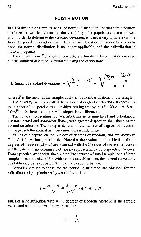
f-DISTRIBUTION
In all of the above examples using the normal distribution, the standard deviationhas been known. More usually, the variability of a population is not known,and in order to determine the standard deviation, it is necessary to take a samplefrom the population and estimate the standard deviation or. Under these condi-tions, the normal distribution is no longer applicable, and the ^-distribution ismore appropriate.
The sample mean X provides a satisfactory estimate of the population mean u,but the standard deviation is estimated using the expression:
. /V1. (IX)2
A IL(X - X)2 \ 2^ nEstimate of standard deviations = \/ = \/
V w - I V n - 1
where X is the mean of the sample, and n is the number of items in the sample.The quantity (n — 1) is called the number of degrees of freedom. It represents
the number of independent relationships existing among the (X-X) values. Since(X-X) = O, there are only n — l independent differences.
The curves representing the ^-distributions are symmetrical and bell-shaped,but not normal and somewhat flatter, with greater dispersion than those of thenormal distribution. Their shapes depend on the number of degrees of freedom,and approach the normal as n becomes increasingly larger.
Values of t depend on the number of degrees of freedom, and are shown inTable A-3 for various probabilities. Note that the lvalues in the table for infinitedegrees of freedom (df = a) are identical with the Z-values of the normal curve,and the entries in any column are obviously approaching the corresponding Z-values.From a practical standpoint, the dividing line between a "small sample" and a "largesample" is sample size of 30. With sample size 30 or over, the normal curve tableor t table may be used; below 30, the t table should be used.
Formulas similar to those for the normal distribution are obtained for the^-distribution by replacing cr by s and z by t\ that is:
J P - u X-Uit = = -p- (with n-ldf)
SX slVn
satisfies a ^-distribution with n—l degrees of freedom where X is the samplemean, and as in the normal curve procedure,

CONFIDENCE LIMITS FORTHE POPULATION MEAN
The ^-distribution is convenient for use in estimating limits for the populationmean. If we solve the following equation for /JL,
±t = * S
V^we find:
» = x±-Vn
which provides lower and upper limits for the population mean JJL with a degreeof confidence depending upon the value selected for t. These are referred to as theconfidence limits for fju.
To find the 95% confidence limits for jn, select the value of t from Table A-3in the Appendix in the column headed 0.05 with n — 1 degrees of freedom (oftendenoted by tn _ 1,0.05)- Similarly, 99% confidence limits would be found by usingthe f-value found in the column headed 0.01 (i.e., tn— 1,0.01).
Example 1A cannery is supposed to be filling cans with 19.0 ounces of fruit. To check conformanceof a new machine with this standard, a random sample of 5 cans is selected from the newmachine's production, and its mean is calculated. If the drained weights of the sample are18.6, 18.4, 19.2, 18.3, and 19.0, can one be 95% sure that the production standard is beingmaintained on this machine? (This is equivalent to asking whether 19.0 is between the 95%confidence limits found for //,.)
X (X-X) (X-X)2
18.6 -0.1 0.0118.4 -0.3 0.0919.2 0.5 0.2518.3 -0.4 0.1619.0 0.3 0.09
93.5 O 0.60
X = 93.5/5 = 18.7

Figure 4-18. Example 1 curve.
From Table A-3,'4,0.05 = 2.776
Therefore,^ = 18.7 ± (2.776)(0.1732) = 18.7 ± 0.48 = 18.22
and 19.18 and since 19.0 is between these two 95% confidence limits, the machine is con-forming (see Figure 4-18).
Example 2The drained weights (in ounces) of a random sample of 9 cans of cherries are as shown.Find the 95% confidence limits for the mean weight of the entire lot.
X (X-X) (X-X)2
12.1 O O11.9 -0.2 0.0412.4 0.3 0.0912.3 0.2 0.0411.9 -0.2 0.0412.1 O O12.4 0.3 0.0912.1 O O11.7 -0.4 0.16
108.9 O 0.46
X = T = 1 2 1
,, Jf =0.24; * = -^ = = 0.08V 8 Vn \/9
95% confidence limits for ^L: X ± %>.055x
12.1 ± (2.306)(0.08) = 12.1 ± 0.18 - 11.92 and 12.28

Therefore, one can be 95% certain that 11.92 ounces to 12.28 ounces willcontain the mean of the lot from which the sample came.
STATISTICAL HYPOTHESES—TESTING HYPOTHESES
Frequently we are required to make a decision about populations based on dataobtained from samples. For example, we may be interested in knowing if one lot isbetter than another, or if one production line manufactures better material thananother. In order to reach such a decision, it may be useful to start with guesses orassumptions about the two populations. Such an assumption is known as a statisticalhypothesis. A statistical procedure or decision rule which leads to establishingthe truth or falsity of a hypothesis is called a statistical test. Decision rules enable theinvestigator to attach to his decisions probability statements about possible outcomesif the experiment were to be repeated many times under the same conditions.Decision rules are also referred to as tests of significance, or tests of hypotheses.
The hypothesis to be tested, often denoted by HQ, is called the null hypothesissince it implies that there is no real difference between the true value of thepopulation parameter and its hypothesized value from the sample. For instance, ifwe wish to determine whether one process is better than another, we wouldformulate the hypothesis that there is no difference between the two processes,and that whatever differences were observed were merely due to fluctuations insampling from the same population. Any hypothesis which differs from H0 iscalled an alternate hypothesis, and is denoted by H\.
In Figure 4-19, the yield for process A is designated by the shaded portionlabeled A. After a change is made in the process, the results are plotted in theportion of the chart labeled B. The null hypothesis Ho states that if the B processfalls within the shaded area, then it is no different than process A. The alternatehypothesis HI states that if the process should fall outside of the shaded area, thenthe two processes are different. This very simplistic example has limited useful-ness since it does not consider probabilities, but it should illustrate the meaningsof the two types of hypotheses.
To test the null hypothesis, one assumes that it is true and examines the con-sequences of this assumption in terms of a sampling distribution which dependson it. If we should find that the results obtained from a random sample are vastlydifferent than those expected under the hypothesis, we would conclude that theobserved differences were significant, and we would reject the hypothesis. As anexample: if 100 tosses of a coin produced 83 tails, we would be likely to rejectthe hypothesis that the coin is fair.
The level of significance of a statistical test defines the probability level awhich is the critical value in decision-making. It is the dividing line betweenaccepting and rejecting. In the event that the calculated probability is less than a,the hypothesis is considered false, and the result is termed significant. It iscustomary to consider a result significant if the probability is less than a = 0.05,and to term it highly significant if the calculated probability is less than 0.01.

Figure 4-19. Null hypothesis for process A and process B.
An alternate hypothesis is any hypothesis other than /T0, and is denoted by H1.IfHi is adopted as the alternative hypothesis, then rejection OfTf0 may be regardedas a decision to accept H\.
If the area of only one tail of a curve is used in testing a statistical hypothesis,it is called a one-tailed test. Similarly, if the areas of both tails are used, the testis referred to as two-tailed. Instead of calculating probabilities, one can comparethe calculated values of Z with those shown in Figures 4-20 and 4-21. A calculatedvalue which is greater than those shown indicates rejection of the null hypothesis.
The values for Z may be selected from the table of normal curve areas. The crit-ical values for Z most frequently used are for probabilities of 10%, 5%, and 1%.These critical values for Z for both one- and two-tail tests are tabulated below:
a (Level of Significance) 0.10 0.05 0.01Z for one-tailed test -1.28 -1.645 -2.33
or +1.28 or +1.645 or +2.33Zfor two-tailed test -1.645 -1.96 -2.58
and+1.645 and+1.96 and+2.58
In testing statistical hypotheses there is no absolute certainty that the conclu-sion reached will be correct. At the 5% level, we are willing to be wrong once in20 times, and at the 1% level, once in 100 times. If we are not willing to chancea wrong conclusion this often, we must select an even smaller value for a. Twotypes of incorrect conclusions are possible. If the hypothesis is true but the sampleselected concludes that it is false, we say that a type 1 error has been committed.The probability of committing a type 1 error is the relative frequency with which wereject a correct hypothesis, and this is precisely equal to the significance level a.
If it happens that the hypothesis being tested is actually false, and if from thesample we reach the conclusion that it is true, we say that a type 2 error has beencommitted. The probability of committing a type 2 error is usually denoted by /3.For a given number of observations it can be shown that if a is given, /3 can bedetermined, and that if a is decreased, /3 is increased, and vice versa. If wewish to decrease the chances of both types of error at the same time, it can be
PROCESS VIELD
Hi (Alternate Hypothesis)
NullHypothesis
Hj(Alternate Hypothesis)
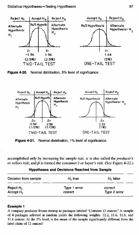
Figure 4-21. Normal distribution, 1% level of significance.
accomplished only by increasing the sample size, a is also called the producer'sor sellers risk; and /3 is termed the consumers or buyers risk. (See Figure 4-22.)
Hypotheses and Decisions Reached from Sample
Decision from sample H0 true H0 false
Reject H0 Type 1 error correctAccept H0 correct Type 2 error
Example 1A company produces frozen shrimp in packages labeled "Contents 12 ounces." A sampleof 4 packages selected at random yields the following weights: 12.2, 11.6, 11.8, and11.6 ounces. At the 5% level, is the mean of the sample significantly different from thelabel claim of 12 ounces?
Figure 4-20. Normal distribution, 5% level of signific#nce.
TWO-TAILTEST ONE-TAILTEST
TWO-TAILTEST ONE-TAILTEST
Reject H0 Accept H0 Reject H0
AlternateHypothesisH1
Null Hypoth AlternateHypothesisHi
Accept H0 Reject H0
Null Hypothesis AlternateHypothesis- H
Reject H0 Accept H0 Reject H0
AlternateHypothesisH1
Null Hypoth AlternateHypothesisHi
Accept H0 Reject H0
Null Hypothesis AlternateHypothesis- H

Figure 4-22. Relation of a and /3.
Null Hypothesis Alternate hypothesis
HQ:fjL = 12ounces H1'.JJL 3= 12ounces
X ( X - X ) (X-X)2
s = , № - X)* = . /024 = V6-^
12.2 0.4 0.1611.6 -0.2 0.04 s V008 r—-
11.8 O O S^=V=n=~V^=V^2 = Q'14
11.6 -0.2 0.04
47 2 o 0.24 *005 = 3'0 5 = 3.182
X =47.2/4 = 11.8 ouncesX± t^Q5sx = 11.8 ± 3.182(0.14)
= 11.8 ±0.45
or
M ± t3t.osSx = 12.0±0.45
Therefore, there is no significant difference between X and JJL.
Example 2A new machine in a cannery is supposed to be filling cans of pears with a standard weightof 19.0 ounces. To check conformance with the standard, a sample of five cans is selectedat random from the production line and its mean is calculated. The drained weights of thesamples are shown below. Is the sample average significantly different from the standardat the 5% level?
DistributionUnder H0
DistributionUnder H1
Acceptance region for HQ Rejection region for H

X (X-X) (X-X)2 M-19.0 Two-tailed
HQ\X = n H1IX^fJL18.6 -0.1 0.01 (Null) (Alternate)18.4 -0.3 0.0919.1 0.4 0.16 - 218.9 0.2 0.04 52 = f^_ ^L = 034 = Q Q85
18.5 -0.2 0.04 /i ~ 1 4
93.5 O 0.34
X = 93.5/5=18.7 Sx=*=^l = y^ = Q 13
From Table 4-3, f0.o5(4 df)=f4>o.o5=2.776
95% confidence limits for JJL: X + 0 05 5^= 18.7 + 27776(0.13)= 18.3419.06
J M=19.0
I ZT"! IE—I18.34 X=18.7 19.06
The sample is not significantly different than the standard. There are two other possiblesolutions to this problem.
(a) Find the region within which X is not significantly different from IJL at the 5% levelof significance.
± , = *^SX
X = IL ± tQQ5Sx ^0.05 = 2.776
= 19.0 ± 2.776(0.13)
= 19.0 ± 0.36 - 18.64 and 19.36
IJM 8.7U 1 1
18.64 ]J= 19.0 19.36Region vithin which X is not Isignificantly different from JJL
^ ^i
(b) From the sample mean, find the region within which the population may be expectedto fall 95% of the time.
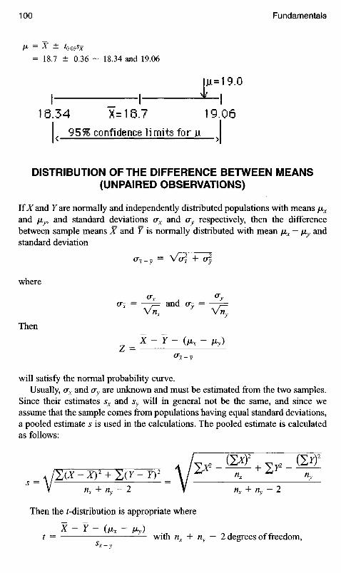
DISTRIBUTION OFTHE DIFFERENCE BETWEEN MEANS(UNPAIRED OBSERVATIONS)
If Xand Fare normally and independently distributed populations with means ^x
and iJLy9 and standard deviations ax and cry respectively, then the differencebetween sample means X and Y is normally distributed with mean ^x — /jLy andstandard deviation
<r-*-y = Voi + of
where
<rx <ry<TX ~ —7= and (Ty = —7=V ; ' v^
Then
X - ? - Ou, - M3)Z =
Vx-y
will satisfy the normal probability curve.Usually, (Tx and ay are unknown and must be estimated from the two samples.
Since their estimates sx and sy will in general not be the same, and since weassume that the sample comes from populations having equal standard deviations,a pooled estimate s is used in the calculations. The pooled estimate is calculatedas follows:
. /__G^ + y72 G£^/I(^y)2 + 2(r-io2
= \ 2^ *x L
V w^ + W7 - 2 V /Ix + ny - 2
Then the ^-distribution is appropriate where
X - Y - (fJL, - IJLy)
t = with nx + ny — 2 degrees of freedom,Sx-y
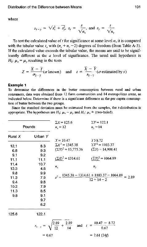
where
S;.y = V^ + 4 ^ = -F=, and Sy = —7=Vnx vny
To test the calculated value of t for significance at some level a, it is compared
with the tabular value ta with (nx + ny—2) degrees of freedom (from Table A-3).
If the calculated value exceeds the tabular value, the means are said to be signif-
icantly different at the a level of significance. The usual null hypothesis is
H0: /Jix = №y resulting in the tests
X — IP X — FZ = (<T known) and t = (a estimated by s)
°"x-y Sx-y
Example 1To determine the differences in the butter consumption between rural and urbanconsumers, data were obtained from 12 farm communities and 14 metropolitan areas, asindicated below. Determine if there is a significant difference in the per capita consump-tion of butter between the two groups.
Since the standard deviation must be estimated from the samples, the ^-distribution isappropriate. The hypotheses are H0: ^x = fjiy and H\. JJLX =1= (two-tailed).
Pounds
Rural X
12.16.89.1
11.111.413.39.8
11.39.4
10.211.39.8
125.6
Urban Y
8.39.39.2
11.110.74.69.97.99.87.98.59.19.76.2
122.1

Tabular lvalues (two-tailed from ^-tables—A-3 in the Appendix)
^0.05(24 df) — 2.064
^0.01(24 df) = 2.797
Since t = 2.6l is larger than 2.064 but less than 2.797, there is a significant differencein butter consumption between the two groups of consumers at the 5% level, but not at the1% level.
If the question had been, "Is the per capita consumption of the rural group greater thanthat of the urban group?" the hypothesis would have been HQ: JJLX = fjiy and HI : JJLX > /u^, anda one-tailed test would have been appropriate. Then
Tabular t-values (one-tailed from /-tables—A-3 in the Appendix)
^0.05(24 df) ~ 1.711
^0.01(24 df) = 2.492
Since / = 2.61 is larger than both 1.711 and 2.492, the per capita consumption ofthe rural group is significantly greater than that of the urban group at both levels ofsignificance.
Example 2Find 95% confidence limits for the mean difference between the performance of two fill-ing machines. Random samples from the two machines A and B gave the following results:
A B
X = 350 g Y = 325 gHX= 10 n_y= 14
2(X-X)2 = 900 2(V- V)2 = 832
2(X - X)2 + I1(Y - Y)2
S2 =
nx + ny — 2
2 900 + 832 1732s = —5— = -w =78-7
then
A /? 7 H /78/7 78/7
*-= V^+ * = VIT +14-= 3-67
95% confidence limits for ^x — fjiy — (X — Y) ± (^22,0.05)^- y
= 25 ± (2.074)(3.67) = 25 ± 7.61= 17.39 and 32.61

- 7.61 + 7.61
17.39 X- Y= 25 32.61
Therefore, we are 95% confident that 17 and 33 grams are limits of the two confidenceintervals which contain the difference in mean filling weights of the two machines. Wethen compare our specification to see if adjustments are necessary.
If instead of ^1(X - X)2 and ^1(Y- Y)2 being given, Sx = 9.5 and sy = 7.7 had been
given, then
/^T ?J 5 _p = A / 1 with nx + nv — 2 degrees of freedomMnx ny
y
= V9.02 + 4.24 = 3.64
PAIRED OBSERVATIONS
Many experiments are performed in such a way that each item of one sample islogically paired with a particular item of a second sample. For example, if mem-bers of a panel of tasters score a sample of each of two similar products, a set ofpaired scores results. With n paired scores of Xand 7, the differences D=X- Yare analyzed.
The mean difference/) =^D/n -X-Y. If the samples are the same,D = O. Thequestion to be answered is, "Is the average difference/) too large for the samplesto be considered as having the same average scores?" To answer this question, onecalculates
t = — with n — 1 degrees of freedom,%
where
„ tl-sjf.WL, № - 5)2 V_ n—s-d = —7= and s = \ = U
Vn V n - 1 V n - 1
The significance of the result is obtained by comparing the calculated value oft with the value from Table A-3 in the Appendix with the appropriate degrees offreedom.
ExampleUsing a 12-point intensity scale, 10 trained judges scored the bitterness intensity oftwo samples of beer as shown below. Do the beers differ significantly in bitterness at the5% and the 1% levels?
HQ : pd = O; HI : /^ =£ O (two-tailed)
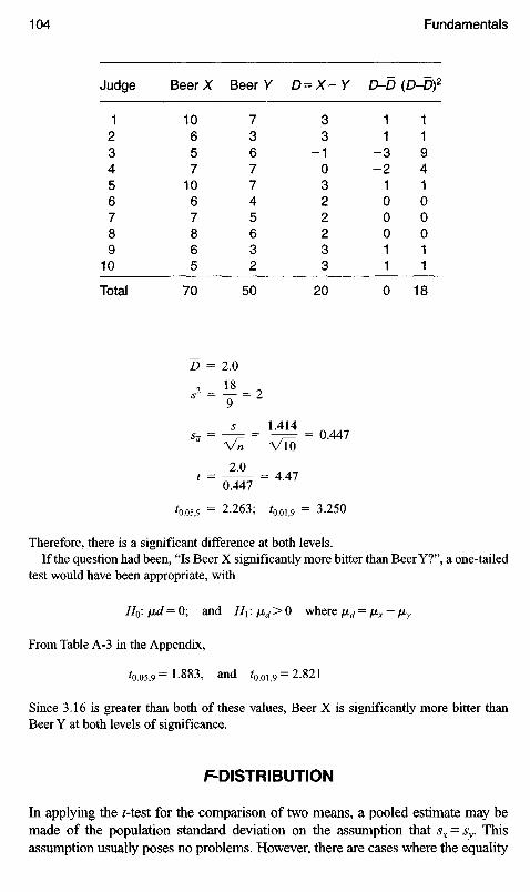
Judge Beer X Beer Y D=X-Y D-D (D-D)2
1 1 0 7 3 1 12 6 3 3 1 13 5 6 - 1 - 3 94 7 7 0 - 2 45 1 0 7 3 1 16 6 4 2 0 07 7 5 2 0 08 8 6 2 0 09 6 3 3 1 1
10 5 2 3 1 1
Total 70 50 20 O 18
Z) = 2.0
2 I** = T = 2 -
5 1.414J3 = —= = —7= = 0.447
Vn VlO
'=0^7= 4 ' 4 7
^0.05,9 = 2.263; faoi)9 = 3.250
Therefore, there is a significant difference at both levels.If the question had been, "Is Beer X significantly more bitter than Beer Y?", a one-tailed
test would have been appropriate, with
H0: ^d = O; and HI : jjid > O where /^ = fjLx — fjuy
From Table A-3 in the Appendix,
^0.05,9 = 1 -883, and fo.oi,9 = 2.821
Since 3.16 is greater than both of these values, Beer X is significantly more bitter thanBeer Y at both levels of significance.
F-DISTRIBUTION
In applying the Mest for the comparison of two means, a pooled estimate may bemade of the population standard deviation on the assumption that sx = sy. Thisassumption usually poses no problems. However, there are cases where the equality
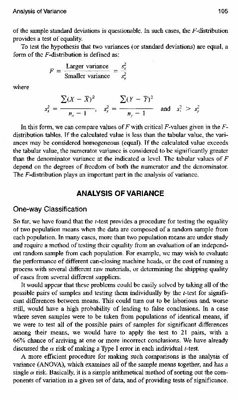
of the sample standard deviations is questionable. In such cases, the F-distributionprovides a test of equality.
To test the hypothesis that two variances (or standard deviations) are equal, aform of the F-distribution is defined as:
__ Larger variance _ s2x
Smaller variance s2
where
^(X-X)2 2(Y-Y)2
s2x = , s2
y = — and s2x > s2
nx-\ y ny - 1 y
In this form, we can compare values of F with critical F-values given in the F-distribution tables. If the calculated value is less than the tabular value, the vari-ances may be considered homogeneous (equal). If the calculated value exceedsthe tabular value, the numerator variance is considered to be significantly greaterthan the denominator variance at the indicated a level. The tabular values of Fdepend on the degrees of freedom of both the numerator and the denominator.The F-distribution plays an important part in the analysis of variance.
ANALYSIS OFVARIANCE
One-way Classification
So far, we have found that the /-test provides a procedure for testing the equalityof two population means when the data are composed of a random sample fromeach population. In many cases, more than two population means are under studyand require a method of testing their equality from an evaluation of an independ-ent random sample from each population. For example, we may wish to evaluatethe performance of different can-closing machine heads, or the cost of running aprocess with several different raw materials, or determining the shipping qualityof cases from several different suppliers.
It would appear that these problems could be easily solved by taking all of thepossible pairs of samples and testing them individually by the /-test for signifi-cant differences between means. This could turn out to be laborious and, worsestill, would have a high probability of leading to false conclusions. In a casewhere seven samples were to be taken from populations of identical means, ifwe were to test all of the possible pairs of samples for significant differencesamong their means, we would have to apply the test to 21 pairs, with a66% chance of arriving at one or more incorrect conclusions. We have alreadydiscussed the a risk of making a Type I error in each individual /-test.
A more efficient procedure for making such comparisons is the analysis ofvariance (ANOVA), which examines all of the sample means together, and has asingle a risk. Basically, it is a simple arithmetical method of sorting out the com-ponents of variation in a given set of data, and of providing tests of significance.
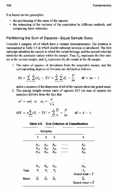
It is based on two principles:
• the partitioning of the sums of the squares• the estimating of the variance of the population by different methods, and
comparing these estimates.
Partitioning the Sum of Squares—Equal Sample Sizes
Consider k samples, all of which have n variates (measurements). The notation issummarized in Table 4-5 in which double subscript notation is introduced. The firstsubscript identifies the sample to which the variate belongs, and the second subscriptidentifies the particular variate within the sample. Thus X2\ represents the first vari-ate in the second sample, and Xy represents theyth variate in the /th sample.
1. The sums of squares of deviations from the respective means, and thecorresponding degrees of freedom are defined as follows:
ss = 2 ^1(Xy - X ) 2 = ix -T: df = fci - iz = i y = i i = i y = i kn
and is a measure of the dispersion of all of the variates about the grand mean.2. The among sample means sums of squares SST (or sum of squares for
samples) follows from the fact that
o2 = no± or a- = -?—Vn
k k T2 T2
SST = n^(Xi -X)2= 2— - — df = k - 1/Ti / = i » kn
Table 4-5. One Criterion of Classification
Samples
1 2 3 k
Total
Mean
X11
X1 2
XI 3
X-\n
T1
X1
x%\X22
%23
X2n
T2
X2
X3,
x$2^33
Xsn
T3
X3
x*iXk2
Xf<3
Xkn
Tk
Grand total = T
Xk
Grand mean =X

3. The within-sample sum of squares SSE (or sum of squares for error) is thepooled sum of squares obtained within each sample, and the pooled valueis unaffected by any differences among the means.
»-[?,*-T] + L^-T]+-^-7]k n k j2
= 224- ST df=k(n-l)I = I j = I i = 1 n
This quantity is known as the experimental error and is a measure of the vari-ation which exists among observations on experimental units treated alike. Fromthe above expressions, it is seen that
SS = SST + SSE
and the same relationships hold for the corresponding degrees of freedom.Because of this relationship, it is customary to obtain SSE as the differenceSS — SST, and the same with the degrees of freedom. These relationships showthat we can always partition the total dispersion in such data into two components,one due to the dispersion existing among the sample means and the other due tothe dispersion existing within the samples.
From the sums of the squares and degrees of freedom, we can obtain two esti-mates of the variance o2. They are
7 SST , SSE* = (F=T) and '--4(F=T)
The first of these is influenced by differences among means, whereas the secondis independent of any differences; therefore any difference existing between thesetwo estimates of o2 is the result of differences among sample means. The twoestimates may be tested for a significant difference by calculating
F=**.
If s2 is significantly greater than s2, significant differences among means areindicated.
The correction term for the set of variates is defined as
C=T2/kn
which occurs in the calculations of both SS and SST. The calculations in theanalysis of variance are shown in the following example.

Analysis of variance
Source of variation
TotalProductsError
SS df
42.55 1928.30 414.25 15
Mean square
7.0750.95
F
7.45Fvalues at 4 and
^0.05
3.06
^0.01
4.89
1 5 degrees of freedom
Since the calculated value of F= 7.45 is larger than F001 = 4.89, significant differencesamong product mean scores are indicated at both the 5% and the 1% levels. Significanceat the 5% level is usually indicated by one asterisk, and at the 1% level by two asterisks.
If the calculated F-value is not significant, further testing is not required. If, however,the F-value indicates significant differences among means, we need to know where the dif-ferences exist. Two procedures in common use are the Least Significant Difference (LSD)test and Duncan's Multiple Range test.
Difference Testing
Least Significant Difference (LSD). The difference between the meansX andF of two independent samples of the same size «, from a normal population withvariance v = s2, is tested for significance by calculating
ExampleFour scores of each of five products are shown in the following table. Are there significantdifferences among these mean scores?
C =(143)2/20= 1022.45
SS = (1O)2 + (8)2 + • • - + (5)2 + (7)2 -C = 1065 - 1022.45 = 42.55 (19 df)
(36)2 + (32)2 4- (23)2 + (27)2 + (25)2
SST - -— —- -C= 1050.75 - 1022.45 - 28.30 (4df)4
SSE = 42.55 - 28.30 = 14.25
The calculations are usually summarized as shown below.
Products
TotalMean
A10899
369.00
B8798
328.00
C5765
235.75
D8775
276.75
E7657
256.25

_ X- Y = X-Y _ X-Y
*--> \/y^ W2ZV n n V n
where v = s2.If, in this equation, we replace t by ta and solve for X — Y, we have
-X- Y= ta\fc
which is the boundary line between significance and nonsignificance at the alevel, and is called the least significant difference between means, that is,
/2 error variance 2slLSD=>V n B = '«V"^
where n is the sample size and I0. is based on the number of degrees of freedomfor error.
Duncan's Multiple Range Test. This is a newer approach to difference testingand provides a series of shortest significant ranges with which to compare differ-ences between means. The shortest significant range Rp for comparing the largestand the smallest of p means, arranged in order of magnitude, is given byRP = QP
sx> where the values of Qp can be obtained from Duncan's MultipleRanges Tables (Table A-7 in the Appendix). The number of degrees of freedomfor the error variance, and the standard error (standard deviation) of any meandetermined from n individual variates, is
/error variance ^ /-*=v—«—ExampleUse (a) the LSD and (b) the multiple range tests to establish significant differences amongmeans at the 1% level for the data of the analysis of variance example.
In that example, the calculated F= 7.45 was larger than F001 = 4.89, so further testingis justified. The error variance = 0.95.
(a)fo.ou5 = 2.947,and
/2(0.95^LSD = 2.947 - A /— = 2.03
V 4
A B D E C
9.00 8.00 6.75 6.25 5.75

Any two means not underscored by the same line are significantly different, and anytwo means underscored by the same line are not significantly different. At the 1% level,means A and B are not signifcantly different; B, D, and E are not significantly different;and D, E, and C are not significantly different.
(b) v = 0.95; p — number of means being compared; Qp with degrees of freedom forerror from Duncan's Multiple Ranges Table (1% level, 15 degrees of freedom); and
RP — Qp5X = shortest significant range for p means; and
s-x = Vv/n = VO.95/4 = 0.49
Shortest significant ranges:
p : 2 3 4 5Qp. 4.17 4.35 4.46 4.55Hp: 2.04 2.13 2.19 2.23
A B D E C5.00 8.00 6.75 6.25 5.75
Difference of Used to compare
2.04 A & B, B & D, D & E, and E & C2.13 A&D, B&E, andD&C2.19 A & E , andB&C2.23 A & C
The results of both methods were the same.
Unequal Sample Sizes. If unequal numbers of measurements are involvedin the samples, only minor modifications are required in the analysis. The for-mula for SST is replaced by
rr>2 >Ti2 '712 Tp2
SST=- + — + — + . . . + — - Cn\ n n3 Kk
The procedure will be illustrated by the following example.
A B C D
9 10 10 1112 7 8 1016 6 8 715 12 12 7
79
_ _ _ 1452 35 38 65 7=190

Since the calculated F-value is less than the tabular value for 3 and 15 degreesof freedom, no significant difference among the samples is indicated.
Whenever unequal numbers of measurements occur in the samples and theF-value indicates significance, there is no simple way to decide which pairs ofmeans differ significantly. All possible pairs must be tested individually by meansoftheMest.
TWO CRITERIA OF CLASSIFICATION(RANDOMIZED COMPLETE BLOCK DESIGN)
In the case of one criterion of classification, no allowance is made for the effectswhich are common to specific variates in all samples. Where such effects exist, asecond criterion of classification is present. This occurs, for example, in a taste-testing experiment in which each judge scores each sample. This design permitsanother measure of variability, that due to the judges. Then, as before, the totalsum of the squares can be subdivided with the addition of a term (SSB) for thejudges. Then
B\ + Bl + B] + - + BlSS = SST + SSB + SSE and SSB = — -
k
where the B's are total scores for the n judges. The pattern is shown in Table 4-6.
C=(190)2/19=1900
SS = (9)2 + (122) + .» + (9)2 + (14)2 - 1900 = 152
(52)2 (42)2 (38)2 (58)2
SST = -L + 1 - + 2- + —- - 1900 = 50.54 5 4 6
SSE =152-50.5 = 101.5
Analysis of variance
Source ofvariation
TotalSamplesError
SS
15250.5
101.5
df
183
15
Mean square
16.836.77
F
2.49
^0.05
3.29

Computations
(a) Correction term C= 1*1 kn
(b) Total sum of squares SS = XSx! ~ c df = /en - 1' j
k
(c) Sum of squares for samples SST = 2 T?/n - C df = k- 1/ = 1n
(d) Sum of squares for judges SSB - E BJ/k ~ c df = n- 1
(e) Sum of squares forerror = SS - SST - SSB df = (kn- 1) - (k- 1) - (n - 1)
ExampleTo determine which of three Napa Valley Chenin Blanc white table wines had the bestquality, five expert wine judges evaluated each wine using a 20-point evaluation scale. Didthe three wines differ in quality? Did the five judges agree in their evaluations?
C = (237)2/15 = 3744.60
SS = (16)2 + (15)2 + • • • + (16)2 + (16)2 - C= 3757 - 3744.60 = 12.40 (14 df)
Table 4-6. Two Criteria of Classification
Samples (Treatments)
Blocks
123
n
TotalMean
1
Judges*nX-J2
^l 3
l /i
T1
X1
2
X21
^22
^23
^2n
7*2
X2
3
*31
^32
^33
Xsn
7-3X3
k
XMXf<2
X(<3
Xkn
T;XR
Total
61B2
B3
Bn
Grand total = 7Grand mean =X
Judges
ABCDE
Total
Wines
X
1615151616
78
Y
1716161816
83
Z
1514151616
76
Total
4845465048
237
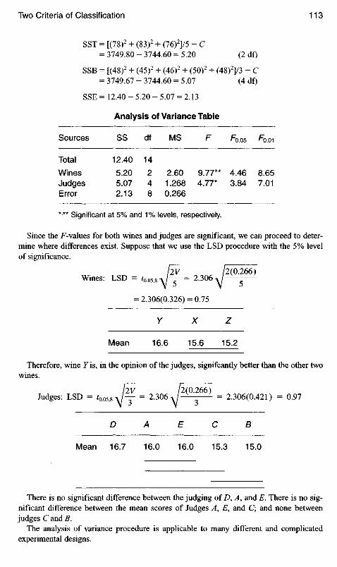
SST = [(78)2 + (83)2 + (76)2]/5 - C- 3749.80 - 3744.60 = 5.20 (2 df)
SSB - [(48)2 + (45)2 + (46)2 + (5O)2 + (48)2]/3 - C= 3749.67 - 3744.60 = 5.07 (4 df)
SSE = 12.40 - 5.20 - 5.07 = 2.13
Analysis of Variance Table
Sources SS df MS F F0-0S F001
Total 12.40 14
Wines 5.20 2 2.60 9.77** 4.46 8.65Judges 5.07 4 1.268 4.77* 3.84 7.01Error 2.13 8 0.266
*'** Significant at 5% and 1% levels, respectively.
Since the F-values for both wines and judges are significant, we can proceed to deter-mine where differences exist. Suppose that we use the LSD procedure with the 5% levelof significance.
/2V /2(0.266)Wines: LSD = '0.05,8A/y = 2.306J g
= 2.306(0.326) = 0.75
Y X Z
Mean 16.6 15.6 15.2
Therefore, wine 7 is, in the opinion of the judges, signifcantly better than the other twowines.
/2V /2(0.266)Judges: LSD = f0.o5,8A/— = 2.306A/— = 2.306(0.421) = 0.97
D A E C B
Mean 16.7 16.0 16.0 15.3 15.0
There is no significant difference between the judging of D9 A, and E. There is no sig-nificant difference between the mean scores of Judges A9 E, and C; and none betweenjudges C and B.
The analysis of variance procedure is applicable to many different and complicatedexperimental designs.

5 Sampling
SAMPLING PLANS
In order to measure the quality characteristics of a population, be it a process, aproduct, or a lot, it is usually desirable to select a sample from the population andexamine it. Rarely is it either desirable or even possible to examine 100% of a lotto determine its quality, hence some assumptions must be made so that a rationalsample can be selected which represents the quality of the underlying population.Needless to say, if the sample selected does not represent the underlying popula-tion, then results of examining that sample are meaningless, and can producesome incorrect and perhaps costly conclusions. If a sample of cherries is selectedfrom trees on the southern side of an orchard, a study of the degree of maturity ofthe sample may result in an erroneous conclusion that the orchard is ready forharvesting, whereas the conclusion should have been that only the southern sideof the orchard was mature.
The study of sampling is enormously complex, and yet the results of analysisof possible sampling procedures ultimately lead to only four simply definedparameters:
1. Where is the optimum location of the sampling point?2. How should the sample be taken from the population?3. With what frequency should the sample be selected?4. What is the optimum sample size?
Methods for analyzing the samples once the system has been established, anddecisions to be made regarding the population quality based on the results ofthese analyses, will be discussed later. First, let us consider the factors inherent inpopulations which must be carefully considered so that a reliable sampling plancan be created.
The cherry orchard example above exhibits the need to ensure that the samplerepresents the population, and not merely a portion of it. Unfortunately, the variables

which exist differ from industry to industry, and from product to product. Forexample, selecting a completely representative and random sample of corn fromthe first truckload in the morning, and analyzing the sample for sugar-starch ratio,may provide the plant operations manager with the information required to deter-mine whether to pack whole kernel or cream style—but only for that truckload!Experience might show that the ratio could change drastically in a very few hours,and that subsequent truckloads might no longer be suitable for the processinitially selected. This leads us to the first decision to be made.
WHY SAMPLE?
In the case of the corn, the need for sampling is to establish the sugar-starch char-acteristic of the incoming raw materials so that the process can be fixed. It isessential that a sample be selected in such a way as to ensure that it representssome defined population. If experience has shown that the ratio changes slowlyduring the morning for product from a given acreage, it may be possible to sam-ple from the first, third, and fifth truck from that acreage to establish the ratio,and to observe process drift for the conditions existing on that particular day(wind velocity, temperature, humidity). Thus, a sample can be used to reliablymeasure this one corn characteristic for this morning period. The answer to the"why sample?" question is obvious in this example: it is not possible to determinethe ratio of the entire truckload, and so a few ears are selected at random in sucha manner as to represent the entire population's composition. The difficultiesinherent in this example are apparent because of the wide variations possible fromfarm to farm, from row to row, and even from ear to ear on a single plant. Yet, itis unlikely that a controlled quality canned or frozen corn product could be pro-duced without this critical measurement of the raw material. Many years ago, thetests for suitability conducted in small plants may have consisted of an experi-enced foreman's selecting several ears from each truckload, cutting a few kernelsand chewing them to rate the color, texture, and flavor. Although these tests wereinexact and primitive, the conclusions drawn from the sample were as dependenton the relation of the sample to the lot as the conclusions drawn from today'smore sophisticated testing methods are dependent on the need for a representa-tive sample.
Sampling a tank truck of liquid sugar or corn syrup for concentration is a farsimpler task. It may be shown, for example, that a composite created from 500 ccsamples drawn from the top, middle, and bottom of a tank truck constitutesa consistently representative sample of the entire contents. The mere fact that itis possible to obtain a reliable sample with relative ease, however, is not a validreason to set up a sampling system. The test results should have some meaningfulfunction in the overall product quality system.
If, for example, the tank truck arrives with a certified Brix, and if the processrequires that every batch of product using that syrup must be adjusted to someunique concentration, which is carefully monitored during the process, there may

be no advantage to knowing that each shipment is at the concentration expected.This certainly does not preclude the necessity for periodic monitoring, but largevolumes of data that are not required to control the quality are of no use, andmerely add to the cost of quality operations.
There is a universal definition of sampling: a procedure which is used to drawinferences about a parent population from results obtained in the sample. To theuninformed, sampling is generally considered to be a simple procedure todiscover defects in products, and it does indeed fit that definition on occasion.However, in the examples above, the cherry samples, the corn samples, and thesugar samples were drawn to measure some aspect of the quality of the popula-tion from which they were selected; they were not selected to find defects.
SAMPLES FROM DIFFERENT DISTRIBUTIONS
Randomly selecting samples from a population to determine facts about itscomposition can produce meaningless data if the distribution of data within theentire population is unknown, or if the purpose for which the data is collected isnot clear to the technician obtaining the information. For example, if the heightsof a sample of 100 tomato plants are measured (Figure 5-1), and there are tendeformed plants only 3-in. high, along with 90 plants which vary from 2 to 4 feetin height, an uninformed technician might report the average height of the tomatoplants in the field at 2.7 feet. The average 3-foot height of normal plants wouldbe of more significance if the harvester equipment were to be set according to theaverage height of normal plants.
Representative samples taken from any distribution can be expected also toexhibit characteristics of that distribution. For example, representative samplesfrom a bimodal distribution should also have bimodal measurements. Let usconsider deliveries of shipping cases received simultaneously from two differentplants, with different average bursting strengths, piled together in a plant ware-house. If truly random samples are selected, bursting strength tests of the samplesshould show two peaks (Figure 5-2).
HEIGHT inFEET
3 Feet average height of normal plants2.7 Feet average height of ALL plants
A portion of the 100 tomato plant sample, showing the effectof including deformed plants in the average height calculation.
Figure 5-1. Average height of tomato plants.
•sfr C
N °

Figure 5-2. Distribution of samples from two shipments.
Similarly, samples taken from skewed distributions can be expected to exhibitskewed measurements mirroring the parent population. It should be noted, how-ever, that compositing samples before analyzing, or averaging the results ofgroups of samples, will tend to create normally distributed sample characteristics,thus masking the true character of the population.
SAMPLE SIZE
There are at least five common policies in use to determine the size of sampleselected, and there is a place for each of them. Each policy is intended to satisfytwo goals: the sample should accurately describe the population, and the samplesize should be the most economical to reach this goal.
Sample Size of Zero
There are occasions where a sample need not be drawn at all. Some materials areso incidental to the process that there is no need to examine them. Silicones usedto lubricate conveyor rails might be an example. Or there may be instances wherean uncomplicated raw material received from a reliable supplier will immediatelybe converted to some other form before use, and which may not constitute aparticularly critical step in the process. An example of this might be common saltwhich is to be converted to various brines for grading green peas. Other classesof materials used in quantity but requiring no sampling might be industrial cleaningsolutions and some maintenance supplies. As part of a "just-in-time" productionsystem, the goal of zero raw material inventories is usually accomplished byshifting the quality control back to the supplier. In this case, examination of thesupplier's quality control records eliminates the need for sampling, except ona monitoring basis. By far, the greatest use of a zero sample size quality control
TWOSHiPhENTSOFCASES
BURSTING STRENGTH
SAMPLES FROM ABOVE SHIPMENTS
BURSTING STRENGTH

program is found within operations where a company depends on luck, supplierreputation, or ignorance. The policy statement: "We have never had trouble withthis before, so we need not sample it" makes as much sense as the remark madeby the farmer whose horse suddenly dropped dead: "That's strange; this neverhappened before."
So far we have considered only raw materials. Sampling along the productionline is a step which cannot be avoided if costs are to be minimized. Yet, there aremanagers unable to see the value in avoiding the costs of scrap and rework byspending a far smaller amount of money in controlling the process quality toavoid making mistakes. It is difficult to conceive of a situation in which it wouldnot be more expensive to correct a faulty finished product than it would be toavoid making the mistake of using an incorrect raw material, or preventing errorsmade on the production line. A zero sampling program of the finished product isunthinkable; yet, it would make more economic sense to reduce the sampling atthe end of the line where mistakes are most costly, and increase the sampling onthe production line and on the raw materials, where errors are less costly. It wouldseem almost axiomatic that a high production record is nowhere as economicallyimportant to a company as a high acceptable quality production record.
100% Sampling
At the other end of the spectrum is a sample size of 100%. In a previous chapter,we have learned that 100% sampling is not effective. Repetitive sampling isboring, and leads to inattention. To demonstrate this point, the author counted allof the "es" in the above paragraph. The first check produced 70. Rechecks counted75, 71, and 87! It is suggested that the reader take on the role of inspector andattempt to decide which figure (if any) is correct.
There are many instances where 100% inspection is considered necessarybecause of the importance of some attribute to the consumer. Packages of multipleunits can be the source of innumerable consumer complaints of missing productunless some method is devised to perform reliable 100% inspection for a correctcount. Tea bags are produced at rates varying from 30 to over 400 bags perminute, and are either machine or hand packaged into cartons of many differentcounts (usually 8, 16, 48, and 100). Even at the lower machine speeds, countingindividual bags for hand-filling operations is tedious work, and makes accuratecounting over an 8-hr shift extremely difficult. Tea bag machine manufacturershave devised counting mechanisms which have greatly reduced the chances for amiscounted package. The machines may be equipped with automatic spacerswhich can be adjusted to nest stacks of 8 or 16 tea bags so that the operator neednot count each bag. The operator places one 8-count stack in an 8-count package,or two 8-count stacks in a 16-count package, eliminating the human error factor.Machines can also be equipped with signal devices to indicate missing bags in thestacks, thus alerting the operator to a possible miscount. As a matter of interest,the 100-count packages are generally designed for three rows of tea bags. Inhand-packaging operations, each row is loaded with 32 bags (from either 4 stacks

of 8 bags, or 2 stacks of 16), and the operator distributes a total of 4 individualbags at the end of the rows to complete the 100-count. The 100% inspection inthese instances is performed by the machine and the operator together, with themost difficult part left to the machine.
Where the units have a substantial weight, 100% inspection for count is sim-plified. Consider a case of 50 packages of 4-ounce trail-mix bags. By determin-ing the tare weight of the empty case plus 50 empty trail-mix bags, the correctcount can be verified by weighing each case on a 25-Ib scale, and comparing theweight to the combined tare plus 12.5 Ib of product. Two precautions are to beconsidered. First, the variation in filler weight deliveries must be controlled;otherwise, 49 packets may be overfilled to such an extent as to produce a casewith the proper gross weight, but with a missing package. Second, a history of thetare weight must be acquired to enable the line supervisor to determine how oftenthe scale setpoint needs to be adjusted for tare variations.
Many other methods have been devised to 100% inspect for counts, eitherdirect or indirect. The sensing device may be an electric eye to produce an electricpulse each time a package trips the light beam; or timing devices which automat-ically speed up a line to separate products; or scaling mechanisms attached to, forexample, condenser plates, thus permitting a change in electric output as a fixednumber of products passes over a point in the production line. Signals to initiateelectronic counting may also be in the form of proximity switches, or contactmicro switches. Each of these, and similar systems, may be tied to counters ordials to verify counts.
Automatic checkweighers are available to 100% inspect the gross weights offilled packages on the production line. These may be equipped with variousdegrees of sophisticated readouts or mechanical devices which can calculatequality control charts for averages and ranges, and which can remove substandardweight packages from the line. Others can be electrically or pneumatically tiedback to the weighing devices so that automatic weight adjustment can be performedby the checkweigher. As above, precautions must be taken to assure that the tarevariations do not interfere with the accuracy of the measuring devices.
Among other 100% inspection devices commonly used are various opticalscanning devices such as the electric eye or the television camera. Infrared or vis-ible light beams are used to test for adequate fill height in rigid containers, and todetect cocked or missing package labels. There is no limit to the list of ingeniousdevices which may be applied to the 100% inspection concept to dramaticallyimprove the reliability of testing compared to that of the human inspector.
It must be emphasized that no mechanical or electrical system for 100% testingcan be installed and allowed to operate without periodic monitoring. The laws ofvariability which these mechanisms are investigating also apply to the devicesthemselves. Gears wear, mechanisms stick, metal fatigues, tubes burn out,connections loosen, electric current varies, levers expand and contract withtemperature, and pivot points wear.
In a method analogous to the one used to determine sampling frequency, aperiodic audit system should be developed by which the testing device can be
evaluated before it would normally be expected to allow measurements to drift.The audit should consist of some reliable secondary standard which has provenreliability.
Spot Checking
A quality control system using only spot checking is doomed to failure. Similarly,a quality control system set up without the additional use of occasional spotchecking is on shaky ground. A spot check is an infrequent, nonscheduled extraexamination of a process or product to reassure the inspector that no mistakes aremade, and to reassure management that the system is working.
Spot checking can also uncover defects in the quality system. In a plant pro-ducing beverage syrups, one of the periodic tests was determination of pH. Thequality control supervisor made an informal spot check every other day or so,using a hand-held pH meter. After dozens of uneventful spot checks, the supervi-sor found a major discrepancy between his reading and that of the line technician.A detailed review of the technician's procedures revealed that the sample hadbeen correctly removed from the line, and that the steps required to place thesample in the meter and to take a reading had also been according to instructions.The problem was solved when it was discovered that the buffering agent used tocalibrate the meter had somehow become contaminated, with resulting incorrectreadings. Fortunately, the plant operated under a batch system, and the few affectedbatches were isolated and adjusted. As a result of this spot check, the procedurefor pH determination was revised to include an extra step for affirming theaccuracy of the buffer against a secondary standard.
Spot checks should not take the place of quality audits. A quality audit isa rigorous procedure to insure that all aspects of a quality system are workingsatisfactorily A spot check may be conducted by anyone at any time, using anytype of examination as an informal test of a fraction of the quality system, buthas no statistical significance.
Constant Percentage, Square Root
One might expect that replacing the haphazard approach of the spot sample withsome sort of systematized sample would be an improvement and it frequently is.Without a statistical approach, it is unlikely that a rational system can be devisedto provide—with a high level of confidence—a sample that describes the qualitylevel of a population. Short cuts to statistical determination of sample size areconvenient and are easy to explain, but they are rarely reliable.
One such short cut is the use of a constant percentage method. There is nocommon rule to establishing the percentage. A small percentage is selected if thepopulation (lot size) is large, if quality variation is expected to be minimal, if thesamples are to be examined by destructive tests, if the testing is time-consumingor costly, or if the population is made up of expensive units. Conversely, a largepercentage is selected if the lot is small, quality is probably nonuniform, testing

is simple or inexpensive, or the units are not costly. The errors inherent in sucha system should be apparent.
Consider the size of sample required to determine the quantity of oxygen ina tank of liquid nitrogen to be used for gas-packaging peanuts.
• The sample will be discarded after testing• The population (cubic feet of gas) is large• The oxygen is uniformly dispersed through the tank• Sampling and testing a large number of samples would be costly.
Even though the last condition (expensive units) is not met, certainly all of theother conditions would dictate taking a single or perhaps duplicate samples of avery small quantity of gas from the tank. A one-cubic-foot sample might typicallyrepresent 0.001% of a small tank's contents. Because of the uniformity of thepopulation, the results of testing this small sample would provide a reliable pictureof the gas quality level.
"Small" means something quite different for different products. A 4,000-lbtruckload of pineapples might seem to satisfy the conditions for small percentagesampling, but 0.001% sampling would amount to perhaps one pineapple pertruckload, certainly not enough to determine the number of moldy fruits present.If there are 1,000 fruits on the truck, a reasonable number to select might be 10.In this case, a "small" sample would be 1%.
There remain two gnawing doubts about the selection of percentage forsampling: (1) Would a 1% sampling method detect moldy fruit if it were presentat 2 per 100; or at 6 per 100? and (2) Should trucks from ranches with a historyof lower quality be subjected to a higher percentage sampling plan than those withhigher quality?
Consider question 1. If 2% of the fruit were moldy, there would be 0.2 moldypineapples in the sample of 10; and there would still be less than a wholemoldy fruit (0.6) in the sample if the quality level were three times as poor(6 moldy fruits per 100). In fact, if the sample of 10 disclosed one moldy pineapple,it would indicate that the truck contained 10% mold, and this might be far toohigh to be acceptable. Perhaps a sample of 1% is not the correct number.
Intuitively, one might answer question 2 affirmatively. On the other hand, alarger sample might not be required for poorer quality since the defects wouldmore easily be found. The problems with the use of an arbitrary sampling planshould now be apparent.
In an effort to improve on the percentage sampling techniques, some advocatethe use of the square-root method (Table 5-1). Again, this is a simple method,easily explained to management, which requires smaller sample sizes for largelots than does the percentage sampling scheme. The following is an example ofthe sample sizes required on two production lines running the same product indifferent sizes. It assumes that samples will be drawn every hour.
In spite of the convenience of the square-root system, there is little to be saidfor its selection. It has no relationship to the number of defects in the lot, and has

no statistical basis for establishing the confidence level of the results. It assumesthat a sample size determined solely by the square root of the lot size has equalability to distinguish between lots with 0.25% defectives and lots with 6% defec-tives. Unfortunately this is not true. There is no rational expression for the resultsof testing lots by this method other than to state that there were x defectives in thesamples, or that the values for ;c in the samples tested ranged from y to z. It is notpossible to state the level of quality using this method except to state that the lotpasses or fails some arbitrary values.
Statistical Samples
So far we have discussed some of the difficulties associated with types of sam-pling procedures, and have implied that there is no way to be sure of the qualitylevel of the population from analyzing samples obtained by using these proce-dures. However, by the use of statistical sampling techniques, it is possible todescribe the quality of the population from which the samples were drawn, and todefine the probabilities associated with the correctness of that evaluation. Thetechniques used in statistical sampling procedures will be described in detail inthe discussion of operating characteristic (O.C.) curves later in this chapter.Statistical sampling procedures answer two very difficult quality questions:
1. How big a sample is required to define the quality of a population?2. Based on the sample characteristics, is the quality of the parent
population satisfactory?
HOWTOTAKE SAMPLES
Sampling procedures must be tailored to the nature of the population being eval-uated. The concept of a random sample seems clear enough: a random sample isone which has been chosen by a process designed to give every item in the pop-ulation an equal chance of being chosen. If the population has satisfactory andunsatisfactory product scattered uniformly, then simple random sampling is effec-tive. If the population is divided into small subgroups each containing product ofuniform quality, then clustered random samples are indicated. If the population
Samples required
Packagesize
1 gallon1 quart1 pint
Productionrate
12/min80/min
200/min
Cans perhour
7204,800
12,000
3% Plan
22144360
Squareroot
2769
109
Table 5-1. Square Sampling Plan

consists of layers of good quality and layers containing defects, then stratifiedrandom sampling is required. Establishing the type of population is usuallyaccomplished by observation of the process just prior to the sampling point. If thetype is not easily determined by observation, analysis of groups of samples takenthroughout the population will readily define it.
Simple Random Sample
To examine the differences between these types of sampling techniques, let usconsider a lot of 5,000 cans of green peas from which we wish to draw a sampleof 50 cans in order to determine the drained weight. A possible method of creat-ing a simple random sample might be as follows: number each of 5,000 balls witha different integer from 1 to 5,000. Each ball now represents one of the cans ofgreen peas. Place the balls in a drum, mix, and remove 50 of them. Next, numbereach of the 5,000 cans from 1 to 5,000. The numbers on the 50 balls wouldrepresent a simple random sample of the 5,000 can lot. This procedure wouldsatisfy the two requirements for a random sample: (a) every subset of size 50 canbe selected; and (b) every subset of size 50 has an equal chance of being select-ed. Obviously this is an impractical procedure, and only serves to illustrate theprinciple of simple random sampling. A more useful method would be to removea total of 50 cans from the line, one at a time, intermittently, and spread out overthe period required to produce a lot of size 5,000. Some bias is bound to be intro-duced by this compromise procedure: the technician might subconsciously avoidever selecting a sample from the first 25 cans; or might sample more slowly at thebeginning, faster in the middle, and not at all near the end of the 5,000-can run.
The mathematical notation commonly used when referring to the simplerandom sample is as follows:
Population size: NSample size: n
(N\Sample subset: I l
A variation of the simple random sample is the systematic random sample.This is generally known as a l/k random sample, and is obtained by selectingevery &th unit from the population, beginning with a unit selected at random fromthe first k units. Referring to the 5,000-can lot of peas in the example above, weagain would number them consecutively as produced, and separate them intosublots. If a 1% systematic sample were desired, the 50-can sample would haveto be selected in such a way that each of 50 sublots was represented. That meansthat one and only one can should be removed from each sublot of 100 cans. Inorder to be a random sample, the can selected from the first sublot of 100 shouldbe randomly chosen. Let us assume that can number 7 were chosen from the firstsublot. To be a systematic plan, can number 7 should then be selected from eachof the remaining 49 sublots. In other words, once a starting point is selected, every100th can shall be selected, thus generating a total sample of 50 cans.

Note this difference between simple and systematic random sampling: insystematic 1% sampling of a 5,000-can stream of production, there are only100 different sets of 50 cans which may be drawn; in random 1% sampling, anycombination of 50 cans may be drawn. Systematic sampling provides a far moremeager selection of the population. Furthermore, if only the center of eachsubgroup is to be systematically sampled, then there is only one possible set of50 cans which can be selected. On the other hand, a simple random samplingprocedure could conceivably miss the first 200 or 300 cans entirely because of thetrue random nature of the selection; the systematic random sample guaranteesthat each 100 sublots shall be included in the 50-can sample.
Choosing between these two types of sampling techniques might be shown inFigure 5-3.
For uniform batch production, use simple random sampling; for continuousproduction, use systematic random sampling. As with any generality such as this,there are bound to be exceptions, and selection of a system should be tailored tothe characteristics of the production line. If, for example, the cans are filled from6 heads, the diagram above would suggest that only head number 3 will besampled; this may or may not be of importance to the analysis of the subsequentexamination of the samples. If head delivery is to be evaluated, the system shouldbe modified to include each head: select head number 1 for the first sample; headnumber 2 from the next subset; head number 3 from the next subset, etc.Alternatively, all six heads might be sampled for every 800 cans produced—orsome similar system might be randomly selected.
Note in the above example that if one of the six heads were defective, thesystematic random sampling techniques in which each head is examined willquickly detect the problem. On the contrary, it is possible that a simple randomsample system might never select a can from the defective head. But the system-atic random sample system is far from perfect. If the samples are taken startingwith every 800th can, and a defect due to a malfunction in the feed hopper causes
Figure 5-3. Simple random sample and systematic randomsample plans.
5YSTEnATlE RANDOM 5AMPLE
SIMPLEPANDQMSAMPLE
TIME
s = sample= can of product

the peas to stop flowing momentarily in between the regular sampling cycle, thenthe systematic random system might never select a can from this period. Thissuggests that before a sampling procedure is established, the possible causes forthe process going out of control should be listed, and a sampling procedure selectedwhich will detect them.
We have looked at relatively simple examples to illustrate the two types of ran-dom sampling techniques, and have suggested that there are hidden weaknessesin each. This should not imply that the methods are unreliable; instead, it suggeststhat no matter which method is used, it should occasionally be audited by use ofa procedure which is likely to reveal weaknesses if they exist. One final caution:since processes are always subject to improvement or accidental changes, thesampling system should be reviewed periodically to verify its effectiveness inassessing the process quality.
Stratified Random Sample
In its classical form, a stratified population is one which is made up of distinctand nonoverlapping groups with differing characteristics. An example might be ahopper (the population) containing a layer (the strata) of mature (the characteris-tic) blackberries (the group), covered by a layer of slightly reddish immatureblackberries, which in turn are covered with a layer of overripe berries. If samplesare drawn at random, a representative sample of the entire hopper would likelydetermine that the maturity was about average. If samples were drawn from eachstrata, it is likely that the conclusion would be that the bin contained three matu-rities. The sampling technique to be selected would depend upon the processwhich followed the bin storage. If the entire contents were to be mixed into asingle batch, a random sample would suffice; if the contents of the bin wereto be used continuously, a stratified sample would indicate that the end productwould vary as the bin was gradually emptied.
Figures 5-4 and 5-5 illustrate the principle of stratified populations oftomatoes. The pH of each truckload of tomatoes is measured as received at thedock by selecting seven random samples. In this case, each truckload may beconsidered as a strata, and the graph clearly shows the variation as received bothwithin each strata and between each strata. In the second graph, the tomatoes con-tained in five truckloads are considered to be a single batch, and the 35 randomsamples show only an approximate range of variation between strata. As with theblackberry bin in the previous example, if the truckloads are used in sequence,the pH of the processed tomatoes can be expected to fluctuate from 4.2 to 4.1, to4.3, etc. as shown in the stratified sample graph. The information from therandom sample graph merely indicates that the tomatoes should average aboutpH 4.2, and that the process will drift between 4.1 and 4.3. The effect of pH onthe quality of the product being manufactured from these raw tomatoes will deter-mine which data (and thus which sampling technique) is required to control theprocess.

Figure 5-5. Random samples (35 per lot).
Cluster Random Sample
Cluster random sampling is a technique used when the population is naturallydivided into a large number of clusters, where the units within the clusters aresimilar to units between clusters. Under these conditions, a cluster random samplewill yield an estimate of the population mean which is likely to be much moreaccurate than an estimate based on a simple random sample of the same size.
Consider a production line filling a lot of asparagus into 4,800 cans which arethen packed in sequence into 200 cases of 24 cans per case. The cases are thenstacked in the warehouse. If we wish to take a sample of size 50 (1 can per 96 pro-duced), we are faced with a number of decisions. Are the major quality differ-ences to be considered due to variation from can to can, from case to case, fromquarter-hour to quarter-hour (or other) period of production?
A random sample could be taken to establish the overall quality of the lotby randomly selecting 50 cans from the lot. This is far simpler said than done:the cases are relatively inaccessible in their stacks, the cases are probably sealedand would have to be destroyed to obtain the samples, the samples removed would
Figure 5-4. Stratified samples (seven per truck).
Sample Number
Avg
PH
Truck*! Truck *2 Truck *3 Truck *4 Truck *5
Average
PH

Table 5-2. Examples of Choices for Cluster SampleSelection
Cluster size Subsample size Total sample
50 cases 1 can from each 5025 cases 2 cans from each 5010 cases 5 cans from each 505 cases 10 cans from each 50
etc. etc. etc.
have to be replaced with cans bearing the same code numbers, and all 12 cansin each case opened would then have to be repacked and sealed in a new casewhich would have to be properly coded and/or stenciled. After all of this effort,the sample would represent the average quality of the lot, and would not indicatepossible variation between cases or variations occurring over the time intervalproduced.
If the cases are considered to be "clusters," a group of random cluster samplescould be drawn. All of the problems listed above would still be present, but theymight be reduced somewhat. There are many possibilities of arriving at a samplesize of 50, depending upon how many clusters are selected, as is illustrated inTable 5-2.
The variation between clusters is best shown by the use of 50-case-clustersize; the variation within clusters becomes more apparent as the subsampleis increased. As with all sampling plans, the goal of the sampling procedure mustbe established before a rational selection can be made.
It should be emphasized that none of the cluster sampling techniques is thesame as a simple random sample from the 4,800 cans. The cluster techniqueincludes selection of many subsets, which means that there are many subsetswhich are not included in the sample. It is also important to realize that onesampling plan does not necessarily provide representative samples for more thanone variable. If the variable under consideration is the satisfactory glue applicationof the label, then the sample should consist of one can from each of many cases;if the variable is the performance of the sealing rollers, then a representativesample might be obtained by examining half the cans in each of a few cases.
TYPES OF SAMPLES
One of the few generalities found in quality control systems is that samplesfall into two classes: those in which variables are measured, and those in whichattributes are counted. Decisions regarding the quality are based on the degree towhich the variables depart from some normal or desired figure, or the extent towhich the attributes exceed some specified limit.

Variables are product or process characteristics which can be measured.There are thousands of variables which affect the quality of food products. As anexample, consider the variables commonly analyzed to establish the quality ofwheat flour:
Variable Measurement units
Solids Percent solidsMoisture Percent waterCold-water soluble PercentAsh PercentAdded inorganic phosphate Percent calcium phosphateIron mg Fe per poundCalcium mg Ca per poundPhosphorus Percent PCarbon dioxide Percent carbon dioxideFat Percent fatCrude fiber Percent crude fiberAcidity of fat mg KOH per 10O gHydrogen ion concentration pH unitsSugars Percent sucroseProtein Percent proteinLipids Percent lipidsUnsaponifiable residue Percent unsaponifiableStarch Percent starchChlorine in flour fat mg per gram of fatNitrite ppm NBenzoic acid ppm benzoic acidBromates ppm bromateslodates ppm iodatesPigment ppm caroteneDiastatic activity mg maltose per 10 gAlpha-amylase Falling number, secondsProteolytic activity Hemoglobin units per gram
The table above refers to product variables, and applies specifically to wheatflour. In addition to the product variables, there are thousands of process variableswhich may affect the quality of the end product. The following table is far fromcomplete, and is intended only to illustrate the array of variables which may beselected for process control:
Temperature Pressure DensitySpecific gravity Color WeightFlow Texture Oxygen
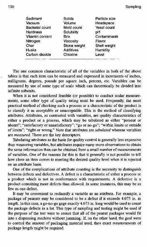
Sediment Solids Particle sizeVacuum Volume HeadspaceBacterial count Mold count Yeast countHardness Solubility pHVitamin content Brix ContaminantsNitrogen Viscosity FlavorChar Stone weight Shell weightHusks Additives HumidityCarbon dioxide Chlorine Level
The one common characteristic of all of the variables in both of the abovetables is that each item can be measured and expressed in increments of inches,milligrams, degrees, pounds per square inch, percent, etc. Variables can bemeasured by use of some type of scale which can theoretically be divided intoinfinite subunits.
When it is not considered feasible (or possible) to conduct scalar measure-ments, some other type of quality rating must be used. Frequently, the mostpractical method of checking such a process or a characteristic of the product isto classify it as acceptable or unacceptable. This is the method of classifyingattributes. Attributes, as contrasted with variables, are quality characteristics ofeither a product or a process, which may be tabulated as either "present orabsent"; "satisfactory or unsatisfactory"; "go or no-go"; "within limits or outsideof limits"; "right or wrong." Note that attributes are tabulated whereas variablesare measured. These are the key descriptors.
Tabulating attributes as the basis for quality control is generally less expensivethan measuring variables, but attributes require many more observations to obtainthe same information than can be obtained from a small number of measurementsof variables. One of the reasons for this is that it generally is not possible to tellhow close an item comes to meeting the desired quality level when it is rejectedon an attribute basis.
One of the complications of attribute counting is the necessity to distinguishbetween defects and defectives. A defect is a characteristic of either a process ora product which is not in conformance with requirements. A defective is aproduct containing more defects than allowed. In some instances, this may be asfew as one defect.
It may be convenient to reclassify a variable as an attribute. For example, apackage of peanuts may be considered to be a defect if it exceeds 4.075 in. inlength. In this case, a go-no-go gage exactly 4.075 in. long would be used to countthe package defects in a lot. This type of sampling and testing might be used ifthe purpose of the test were to assure that all of the peanut packages would fitinto a dispensing machine without jamming. If, on the other hand, the goal wereto control the amount of packaging material used, then exact measurements ofpackage length might be required.

SAMPLING PLANS
The most common procedure used to determine the acceptability of the qualitylevel of a lot is to select a random sample, examine it for one or more qualitycharacteristics, tally the number of defects found, and then decide on acceptanceor rejection of the lot. The sample size may vary from one unit to many, depend-ing upon the size of the lot and the probability of acceptance or rejection.Sampling plans for acceptability of lots are discussed at length at the end ofthis chapter.
When the decision to accept or reject is based on the test results from one sam-ple, the plan is referred to as a single sampling plan. In some cases, rejecting alot on the basis of a single sample may raise doubts in the mind of management,the customer, the vendor, or production personnel. In other cases, a single sam-pling plan requires destructive testing which might be costly. Because of theseconsiderations, it might be desirable to consider multiple sampling procedureswhich start with smaller size samples.
In double or multiple sampling plans, a failure of the first sample to containan acceptable number of defects automatically permits drawing a secondsample (double plans) or in the event that fails, additional samples may be drawn(multiple plans).
There would appear to be justification for double sampling plans where thecosts of running the tests are high, since a lot can be considered satisfactoryon the first small-size sample if it proves to be defect free. On the other hand, ifthe purpose of a double sampling plan is to "give the lot another chance," thenthe principle behind sampling plans is misunderstood.
When a lot is rejected, the news is often received by the production personnelwith little enthusiasm. The first reaction might be "you pulled a bad sample. Takeanother sample and let's see how that one comes out." Depending upon thecircumstances, perhaps the best answer the quality manager can use to respond tosuch a request is "perhaps we should also pull another sample from each of thelast three lots which were found to be satisfactory."
TYPES OF INSPECTION
"Sampling Procedures and Tables for Inspection by Attributes" was originallyissued as a Military Standard Number 105 and is available as MIL STD 105E. Ithas been slightly modified and issued as American National Standard ANSI/ASQCZ 1.4 1981. These standards provide guidance for initiating inspection procedures,as well as instructions on switching to tightened or reduced inspection.
The suggestion that flexible procedures be allowed has been subject to muchdebate. The logic is fairly clear, but the rules for switching from one procedure toanother are arbitrary, and open to considerable question.
The principle seems to be that if a producer has a history of acceptable quality,lots from that producer should be examined by a less stringent procedure. Thestandards state that normal inspection will be used at the start of inspection"unless otherwise directed by the responsible authority." Reduced inspection shallbe instituted providing that all of the following conditions are satisfied:
1. The preceding 10 lots have all been on normal inspection, and have allbeen accepted. (The reason for 10, rather than some other number, is notexplained.)
2. The total number of defects found in the samples from the 10 lots doesnot exceed designated values presented in a table of the standard.
3. Production is at a steady rate. ("Steady" is not defined.)4. Reduced inspection is considered desirable by the responsible authority.
("Responsible authority" is not defined.)
The standards have provided rules to follow in switching from reduced back tonormal, normal to tightened, and tightened to normal. In spite of the arbitrarynature of these rules, the standard is accepted worldwide, and has been very effec-tive in the field of quality control.
CLASSES OF DEFECTS
Many subjects are taught where specific areas are classified to make it easier tolearn. In the case of defect classification, this is certainly true, but there are otheradvantages. For one thing, the interrelationships between classes of defects andtheir respective costs to the company dictate where cost reduction efforts are mostlikely to have the greatest effect. A second need for classification of defects is todetermine which types of defects cause the more severe problems with qualitycontrol, thus dictating which areas need the most attention.
Quality defects are classified into three broad areas: critical, major, and minor.Critical defects are those which are certain to cause failure of the product to func-tion as designed. The most serious of critical defects are the types which canendanger the health of the consumer—contamination by toxic chemicals, salmo-nella, botulinum, metal or ceramic fragments, etc. Other defects which may ormay not directly endanger health may be classified as critical if they cause theproduct to become inedible or distasteful—severely discolored, infested withinsects, moldy, etc. A third type of critical defect is one which is in violation ofthe law, and may not be marketed without risk of severe penalties—unapprovedadditives, deceptive labeling, ingredients exceeding regulatory limits, etc.
The second classification, major defects, is a difficult one to define. It generallyincludes those defects which are likely to have important adverse effects on theappearance or function of the product. Dented cans might appear in this classifi-cation, but the severity of denting could determine the importance of this defect.A dent causing a fracture of the metal would be critical; a dent which is barelydetectable might not be considered a defect at all.
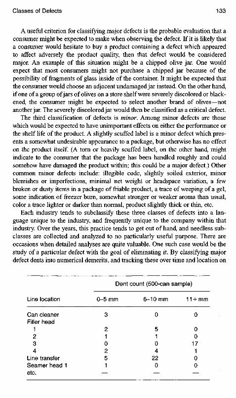
A useful criterion for classifying major defects is the probable evaluation that aconsumer might be expected to make when observing the defect. If it is likely thata consumer would hesitate to buy a product containing a defect which appearedto affect adversely the product quality, then that defect would be consideredmajor. An example of this situation might be a chipped olive jar. One wouldexpect that most consumers might not purchase a chipped jar because of thepossibility of fragments of glass inside of the container. It might be expected thatthe consumer would choose an adjacent undamaged jar instead. On the other hand,if one of a group of jars of olives on a store shelf were severely discolored or black-ened, the consumer might be expected to select another brand of olives—notanother jar. The severely discolored jar would then be classified as a critical defect.
The third classification of defects is minor. Among minor defects are thosewhich would be expected to have unimportant effects on either the performance orthe shelf life of the product. A slightly scuffed label is a minor defect which pres-ents a somewhat undesirable appearance to a package, but otherwise has no effecton the product itself. (A torn or heavily scuffed label, on the other hand, mightindicate to the consumer that the package has been handled roughly and couldsomehow have damaged the product within; this could be a major defect.) Othercommon minor defects include: illegible code, slightly soiled exterior, minorblemishes or imperfections, minimal net weight or headspace variation, a fewbroken or dusty items in a package of friable product, a trace of weeping of a gel,some indication of freezer burn, somewhat stronger or weaker aroma than usual,color a trace lighter or darker than normal, product slightly thick or thin, etc.
Each industry tends to subclassify these three classes of defects into a lan-guage unique to the industry, and frequently unique to the company within thatindustry. Over the years, this practice tends to get out of hand, and needless sub-classes are collected and analyzed to no particularly useful purpose. There areoccasions when detailed analyses are quite valuable. One such case would be thestudy of a particular defect with the goal of eliminating it. By classifying majordefect dents into numerical demerits, and tracking these over time and location on
Dent count (500-can sample)
Line location 0-5 mm 6-10 mm 11 + mm
C a n cleaner 3 O OFiller head
1 2 5 02 1 1 03 O O 174 2 4 1
Line transfer 5 22 OSeamer head 1 1 O Oetc. — — —

the production line, it may be possible to identify the various causes of the defect,thus leading to elimination of those which are most troublesome.
In this simplified, partial study, it should be apparent that there is considerabledamage to the cans at filler head No. 3 and at the line transfer station. The needfor adjustment, maintenance, or possibly redesign is indicated.
It has been suggested that converting the three classifications to numerical termswill permit analysis by statistical means. One such scheme is to apply values suchas 100, 30, and 10 to critical, major, and minor defects. Another suggestion is toapply probable scrap or rework costs to each defect as accumulated. It is difficult toperceive of this type of quality control technique as being particularly useful over along term, but perhaps the use of the dollar analysis for a short-term study mighthighlight the significance of a problem. It might also provide operations manage-ment with data to justify a capital expenditure to improve the product quality.
Two other important systems for classification of defects are the gradingprocedure for raw fruits, vegetables, grains and meats (U.S. Department ofAgriculture [USDA]), and the standards and contaminant regulations for specificfoods (Food and Drug Administration [FDA]). These procedures and standardsare rigorously defined, and rarely (if ever) require statistical analysis for qualitycontrol.
Perhaps a philosophical note would be in order at this point. There will alwaysbe variability in the raw material and the processing of food products. There willalways be defects in food products. Some of these defects are preventable. Sincequality managers and their corporate leaders are humans (for the most part), it canbe expected that here, too, there will be variability in the selection of projects toeliminate defects. Look at some of the choices in selection:
• some will save more money than others• some will not save any money, but will add to costs• some might improve the image of the quality department• some are very interesting projects• some are extremely difficult• some are very important to upper management• some might provide solutions detrimental to others' reputation• some might apply to short-lived products
One of the more powerful statistical tools used to evaluate the list of prioritiesis the Pareto Curve. It suggests that a "critical few" defects produce the bulk ofthe consumer complaints, and that the "trivial many" defects are responsible fora relatively small proportion of complaints. Logically then, the quality departmentcan provide the greatest complaint reduction by eliminating the causes for the"critical few" defects. Often this is the case. But bear in mind that among the"trivial many" defects that cause little concern, there are some defects whichcould cause ruin to the company if they were not controlled rigorously. One cannotignore the constant threat of salmonella even though it is among the "trivialmany" defects which rarely, if ever, appear as a complaint.

If the powerful logic of the Pareto analysis does not always work, how does oneselect the projects to eliminate all of the defects? The answer here is a great dealsimpler than most are willing to admit. Yes, Pareto is powerful, and it is useful.Yes, it is possible to select a project from the above partial list of eight choices.But it is not possible to provide a system which will magically solve all of thedefect problems in one major effort. The control of quality cannot be establishedby formula since each company has unique variables of suppliers, processes,equipment, marketing goals, and (most important) people with unique needs, per-sonalities, and motivation. Projects should be selected in accordance with theneeds as perceived by the company (not by the quality department), and solutionswill be created and implemented one at a time. Quality control and qualityimprovement do not arrive in a bolt of lightning as so many quality programspromise; quality control is established and reestablished one step at a time.Likewise, quality improvement is established one step at a time.
SAMPLING RISKS
The risks associated with acceptance sampling have been classified into fourgroups, two for the producer, and two for the consumer. These can be tabulatedas follows:
Probability of acceptanceProducer (Type I risk); Consumer (Type II risk)
Probability of rejectionProducer (Alpha risk); Consumer (Beta risk)
The first reaction to this classification is that it is unnecessarily complicated,but as we shall see in the discussion of O.C. curves (the technique by which anunlimited number of sampling plans can be derived), it is essential that these risksbe understood.
Both the producer and the consumer would like to accept only perfect lots:zero defects. In some instances, this is an attainable goal, but only at considerableexpense to the producer, and at prices which might be unrealistic to the consumer.Each party has to be willing to reach a decision as to the number of defectiveitems in a lot which would be acceptable. There are no universal rules for deter-mining the acceptable quality level. It is generally arrived at over a long period oftime during which general management, production, quality control, purchasing,accounting, research, and sales all provide inputs until a general consensus isreached. This compromising process is a continuing one. As new needs arise, oras processes, costs and raw materials change, the acceptable quality level may beeither narrowed or expanded.
Having established the acceptable quality level (AQL) both the producer and theconsumer are now faced with an additional decision: how precise a figure is this? Isthere any margin for error? This is where the factor of risk appears. Of course, the
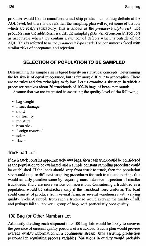
producer would like to manufacture and ship products containing defects at theAQL level, but there is the risk that the sampling plan will reject some of the lotswhich are really satisfactory. This is known as the producer's alpha risk. Theproducer runs the additional risk that the sampling plan will erroneously label lotsas acceptable when they contain a number of defects which is outside of theAQL. This is referred to as the producer's Type I risk. The consumer is faced withsimilar risks of acceptance and rejection.
SELECTION OF POPULATIONTO BE SAMPLED
Determining the sample size is based heavily on statistical concepts. Determiningthe lot size is of equal importance, but is far more difficult to accomplish. Thereare no rules and few principles to follow. Let us examine a situation in which aprocessor receives about 20 truckloads of 100-lb bags of beans per month.
Assume that we are interested in assessing the quality level of the following:
• bag weight• insect damage• mold• uniformity• moisture• bean size• foreign material• color• flavor.
Truckload Lot
If each truck contains approximately 400 bags, then each truck could be consideredas the population to be evaluated, and a simple constant sampling procedure couldbe established. If the loads should vary from truck to truck, then the populationsize would require different sampling procedures for each truck, and perhaps thiswould unfairly penalize some by requiring more intensive inspection of smallertruckloads. There are more serious considerations. Considering a trucklbad as apopulation would be satisfactory only if the truckload were uniform. The loadcould consist of produce from several farms or several warehouses with varyingquality levels. A sample from such a truckload would average the quality of all,and perhaps fail to uncover a group of bags with particularly poor quality.
100 Bag (or Other Number) Lot
Arbitrarily dividing each shipment into 100 bag lots would be likely to uncoverthe presence of unusual quality portions of a truckload. Such a plan would provideaverage quality information in a continuous stream, thus assisting productionpersonnel in regulating process variables. Variations in quality would probably

not be detected by a population definition of this type if the variations were dueto such factors as location of the bags in the truck or in the warehouse precedingdelivery, wherein the product may have been exposed to heat, moisture, light orcontamination.
Pallet-Load Lot
If there is no particular advantage to isolating portions of truckload deliveries, orif the variations between truckloads do not have ah important effect on furtherprocessing in the plant, then the trucks might be unloaded and restacked onpallets in the plant warehouse, and each pallet load might then be considered asthe population. In fact, if the variations are generally unimportant, the populationmight be defined as 2 pallets, or 5 pallets, or a larger number. In this case,composite samples may be obtained from several pallets, thus reducing the costof sampling. Pallets are a convenient population (or subpopulation), but in someinstances, it might be advisable to dump truckloads directly into bins, in whichcase the bin contents become the population.
There appears to be no limit to the size of the population which might beselected to establish the quality level of incoming truckloads of beans. There are,however, a number of guidelines which might be considered. First and foremostis an understanding of which quality factors have to be measured—which qualityfactors are important to further steps in the process. If moisture is critical, a seriesof studies will assist in determining the logical size of the population to be usedroutinely. The first study would be a detailed examination of the variation ofmoisture within a single bag. If it is found that there is no consistent difference inthe moisture levels found at the top, bottom, center, or edges of a single bag, thenthe next series of tests would be detailed examination of the variation of moisturebetween bags. Similarly, if it is found that the moisture variation between indi-vidual bags taken from a single truckload is minimal, then the third series of testswould be to establish differences in moisture level between truckloads. This typeof investigative testing is continued to establish the points at which significantvariations begin to appear. Other possible studies might include differencesresulting from farm-to-farm variation, seasonal variation, temperature andhumidity variations, year-to-year comparisons, etc. Once the level at whichsignificant variations begin to appear is determined, the population size requiredfor quality control sampling for that variable becomes apparent.
There is a likelihood that conditions will eventually change—new trucks,different farms, varietal improvements, different process requirements, improvedpackaging of raw materials. Consequently, the procedure of selecting populationsize must be reviewed periodically to confirm its integrity.
SELECTION OF SAMPLE FREQUENCY AND LOCATION
How often should a sample be selected for quality evaluation? The answer to thisquestion is simple: if the quality variable or attribute to be examined normally
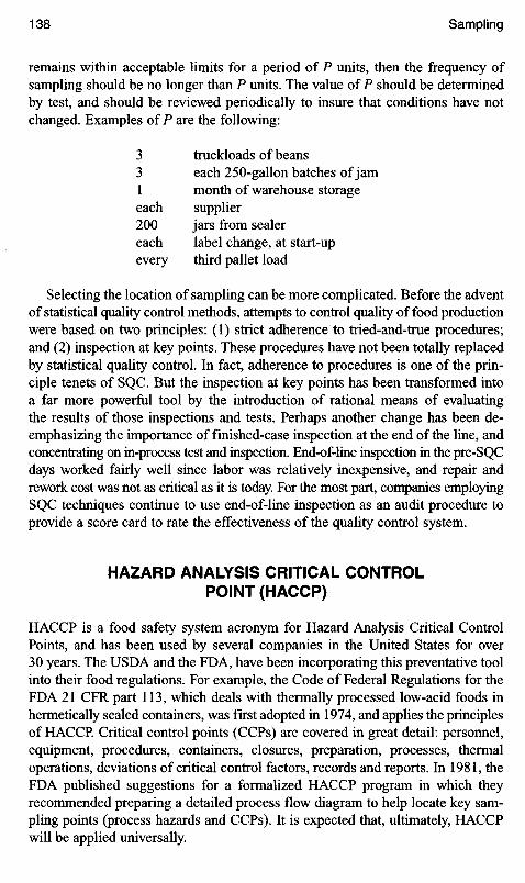
remains within acceptable limits for a period of P units, then the frequency ofsampling should be no longer than P units. The value of P should be determinedby test, and should be reviewed periodically to insure that conditions have notchanged. Examples of P are the following:
3 truckloads of beans3 each 250-gallon batches of jam1 month of warehouse storageeach supplier200 jars from sealereach label change, at start-upevery third pallet load
Selecting the location of sampling can be more complicated. Before the adventof statistical quality control methods, attempts to control quality of food productionwere based on two principles: (1) strict adherence to tried-and-true procedures;and (2) inspection at key points. These procedures have not been totally replacedby statistical quality control. In fact, adherence to procedures is one of the prin-ciple tenets of SQC. But the inspection at key points has been transformed intoa far more powerful tool by the introduction of rational means of evaluatingthe results of those inspections and tests. Perhaps another change has been de-emphasizing the importance of finished-case inspection at the end of the line, andconcentrating on in-process test and inspection. End-of-line inspection in the pre-SQCdays worked fairly well since labor was relatively inexpensive, and repair andrework cost was not as critical as it is today. For the most part, companies employingSQC techniques continue to use end-of-line inspection as an audit procedure toprovide a score card to rate the effectiveness of the quality control system.
HAZARD ANALYSIS CRITICAL CONTROLPOINT (HACCP)
HACCP is a food safety system acronym for Hazard Analysis Critical ControlPoints, and has been used by several companies in the United States for over30 years. The USDA and the FDA, have been incorporating this preventative toolinto their food regulations. For example, the Code of Federal Regulations for theFDA 21 CFR part 113, which deals with thermally processed low-acid foods inhermetically sealed containers, was first adopted in 1974, and applies the principlesof HACCP. Critical control points (CCPs) are covered in great detail: personnel,equipment, procedures, containers, closures, preparation, processes, thermaloperations, deviations of critical control factors, records and reports. In 1981, theFDA published suggestions for a formalized HACCP program in which theyrecommended preparing a detailed process flow diagram to help locate key sam-pling points (process hazards and CCPs). It is expected that, ultimately, HACCPwill be applied universally.

Seven principles of HACCP, adopted by the USDA and the FDA in 1997, are:
1. Conduct a hazard analysis2. Identify critical control points (CCPs)3. Establish critical limits for each CCP4. Establish monitoring procedures for CCPs5. Corrective action6. Verification procedures7. Record keeping and documentation.
• by 1997: Mandated for meat, poultry and seafood plants• Under way: juice, egg
HACCP is recommended by Industry Associations:
International Dairy Foods Assn: milk, ice cream, cheese, yogurt, butterRefrigerated Foods Assn: cole slaw and othersAmerican Spice Trade Assn: whole spices, blended seasoningsAmerican Institute of Baking: bread, buns, cake
Most of HACCP principles were already FDA-enforced in the low-acid cannedfood industry when the first of the regulations were enacted for meat and poultryby the USDA (1998). The FDA issued HACCP regulations for the seafood indus-try (1995), the bottled drinking water and the juice industry (2001). The FDA hasconducted pilot programs for cheese, frozen dough, flour, bread, cereals, saladdressing and other products. It is just a matter of time before all food products areincluded under HACCP regulations.
The Statistical Application to HACCP
HACCP principle No. 3 (establish limits for each CCP) and HACCP principleNo. 4 (establish monitoring procedures) requires control chart analysis. Asexplained elsewhere in this book, either variable or attribute control charts shouldbe used to evaluate the acceptance at each CCP. Dependence on antiquated pro-cedures of periodic inspection will not suffice.
The task of the FDA as food industry regulator is to oversee the food industryto ensure that it meets its legal requirements. For years, the ability for the FDAto assess a food company's performance in meeting its legal responsibilitieswas based on observations of a plant's practices at the moment of regulatoryinspection. The assumption of the inspector was that the plant operations onthe day of the inspection were typical. HACCP thus became a more efficientregulatory tool.
FDA regulations for low-acid canned foods contain many of the HACCP prin-ciples. HACCP regulations for the seafood industry were introduced by the FDAin 1995 under 21 CFR 123, and for the juice industry in 2001, effective in 2002.The USDA established HACCP regulations for meat and poultry products in

1999. It can be expected that before long all food products will require HACCPregulations. The FDA continues to develop HACCP regulations as the food indus-try safety standard for domestic and imported food products. The Food Safety andInspection Service of the USDA defined HACCP as a systematic approach tofood safety. "The primary goal is to assess hazards and risks associated withgrowing, harvesting, raw material and ingredients, processing, manufacturing,distribution, marketing, preparation and consumption of food."
The FDA issued seven principles involved in HACCP:
1. Analyze hazards. Examples: biological, physical contamination, chemical.2. Identify the CCPs. These include processing hazards such as foreign
material contamination, heating, packaging.3. Establish preventative measures with critical limits for each control point.
An example would be cooking time and temperature.4. Establish procedures to monitor the CCPs.5. Establish corrective actions when monitoring indicates failure at a critical
control point.6. Establish procedures to verify that the processing operation is proceeding
according to standards.7. Establish effective record keeping to document the HACCP system. This
should include records of hazards, control procedures, and monitoring.
Some of the advantages of a HACCP system, as expressed by the FDA intheir Backgrounder publication October 2001 apply both to the food processorand to the FDA inspectors. It provides focus on identifying hazards fromcontaminating food and is based on sound science. The record-keeping require-ments provide more efficient government oversight, and help the food proces-sor to compete more effectively in the world market. The need for furtherregulation is indicated by the growth in.the food industry and research projectswhich continue to uncover possible chemical and biological hazards in foodproduction.
It must be emphasized that the HACCP procedures regulate critical healthrisks—not quality control of the food product. Critical Control Point is definedby the USDA as: "Any point or procedure in a specific food system where loss ofcontrol may result in an unacceptable health risk." Other serious quality charac-teristics such as underweights, wrong ingredient, over or under mixing time,incorrect color, strange texture, unusual odor, etc. are not a factor of the HACCPsystem. A suggested procedure for overcoming this potentially serious omissionis discussed later.
First, a process flow diagram (Figure 5-6) is constructed for each product,showing the individual steps in sequence from receipt of packaging and raw mate-rials, through plant processing steps, to final shipment or storage of the finishedproduct. Then each step is analyzed for possible hazards. The FDA defines aprocess hazard as "a possible source of trouble along the processing chain whichmight be defined as a failure to identify: (1) critical materials, (2) critical process-ing points, (3) adverse environmental conditions, and (4) human malpractices."

Figure 5-6. Process diagram of pecan shelling (from FDA model qualityassurance plan).
Once these CCPs have been determined, a sampling system including samplelocation, size, frequency, methods of selection, testing, analyzing and reporting isestablished. From management's point of view, inadequate control of CCPs isundesirable (or even fatal), since it leaves the company exposed to the dangers ofproducing defective products which might, if shipped to the public, adverselyaifect the reputation or the even the financial structure of the company. At thevery least, defective products could result in costly scrap or rework. At the otherextreme are the possibilities of product recall or adverse consumer action.
In addition to these immediate concerns, there are legal considerations as well.Failure to recognize CCPs might result in unacceptable risks of adulteration, or fail-ure to comply with federal, state, or local regulations with respect to net content,food standards, good manufacturing practices, sanitation, or storage conditions.
Figure 5-7 is another example of a HACCP chart. This one is for quality con-trol of empty cans received on pallets, can ends, insert coupons, and plasticresealers. In this application, cases, case glue, coder ink and other case suppliesare handled on a separate HACCP chart, along with other cardboard and flexiblepackaging supplies, and will not be considered here.
The numbers shown after critical equipment refer to standard quality controlprocedures as described in the quality control manual. 1.01 refers to laboratory
(1) RAW MATERIAL INSPECTIONQUALITY CONTROL POINTS
(3) AVAILABLE CHLORINE(2) AVAILABLE CHLORINE, TIME/TEMP (4) TIME/TEMP
(5) E. COLI AND CURCULIO(6) NET WEIGHT
STORAGE
PACKAGING (6)(MECHANICAL OR MANUAL)
(5) HAND PICKINGHAND PICKING (5)
ELECTRONIC SORTERS
SIZER/BLOWER
DRYER (4)
PICKING WHEELS
PECAN HALVES
WASTE SHELL
GRINDER
ATTACHED PECAN IN SHELL
SHELLER AND PRIMARY SIZER
PECAN CRACKER
TEMPERING FOLLOWED BY SANITIZATION AND DRYING (2)
WATER WASH AND DRAINING
LIGHT OR DEFECTIVE NUT REMOVER
WHOLE PECAN SIZER
WHOLE PECANS PRECLEANED
NUTS HELD IN COLD STORAGE
RAW MATERIAL EVALUATION AND PREPARATION (1)
PIECES
SIZER/BLOWER
(3) FLOTATION
(4) DRYER
SIZER-BLOWER/OR PICKER

Figure 5-7. Process diagram of bulk can supplies.
tests for approval of can lithography (color and content), dents, leaks, side seamand throwback solder, leaks, foreign material, scuffs, etc. For those companieswith standardized written operating procedures, another set of numbers mightalso appear on the HACCP chart, referenced to applicable operations to be takenby plant personnel. This might include cursory physical examination, count andtally with receiving documents, checkoff tickets with loads and incoming paper-work, and similar operations documents.
In any business endeavor, the management must be aware of the possible haz-ards in the conduct of the business which will adversely affect the outcome; andthey also realize that some of these hazards are critical to satisfactory perform-ance. To this extent, HACCP is not a unique concept, but it differs from informalprocedures for avoiding mistakes and failures in that it is a detailed system whichincorporates seven distinct areas:
1. Identification of severity of a likely hazard.The FDA and the USDA state that a hazard may be a biological, chemicalor physical property that may cause a food to be unsafe for consumption.
RECElVlNGCANSON PALLETS
1.01
RECEIVINGENDS1,05
RECEIVINGINSERTS
1.07
RECEIVINGLIDS1.11
CAN STORAGE1.02
DEPALLETIZER1.03
AIRCONVEYOR
SEALEDCONVEYOR
SEALEDCONVEYOR
BLOWER
CLEANER1.04
FILLER1.12
CAN SEALER
CASER1.14
WAREHOUSE1.15
END STORAGE1.06
GRAVITYFEEDER
GRAVITYFEEDER
MARKETING1.08
STORAGE1.09
INSERTER1.10
INSERTERUO
LIDSTORAGE1.12
LIDFEEDER1.13
LID FEEDER1.13

Additionally, a commercial hazard is any condition which would make theproduct dangerous or unsalable.
2. Locating the CCPs in which a failure would likely result in a hazard beingcreated or allowed to persist.A CCP is a point or procedure in a food system where loss of control mayresult in an unacceptable product (or in the case of FDA and USDA, anunacceptable health risk). Controls applied at these process steps shallprevent, eliminate, or reduce to acceptable levels the hazards identified.
3. Documenting control limits for each point.Tolerances of safety shall be established for each CCP to control a qualityhazard (defined by FDA and USDA as a health hazard, or multiple healthhazards).
4. Creating a system for monitoring these CCPs.Each CCP shall be controlled through a planned sequence of measure-ments or observations which are recorded for subsequent audit procedures.Continuous (100%) monitoring is recommended, but where it is not pos-sible, the frequency of observation should be determined by statisticallydesigned data collection systems. A system of calibrating the equipment,reagents and instruments used in controlling and monitoring should beincluded. This also applies to validation procedures of software forcomputer control systems.
5. Establishment of corrective actions to be taken.When a critical control limit has been exceeded, the cause of the deviationmust be corrected and eliminated. The materials involved shall be tagged,or otherwise identified, and removed from the process for subsequent dis-position. Each CCP will require specific corrective action in the HACCPplan. Precise records of each deviation and corrective action taken shallbe maintained for the shelf life of the product.
6. Preparing and maintaining records of these observations.A written HACCP plan (manual, procedure) should be prepared, and con-tinually updated. Records generated during operation of the plan shouldbe current and complete. A check sheet consisting of "pass/fail" is notconsidered satisfactory for recording data at CCPs. Instead, actual valuesobtained during monitoring should be recorded, along with productdescription, product code, time and date of data collection. Consumercomplaints relating to CCP should be included in the HACCP records.
7. Providing routine audits of the system to verify its adequacy.Audit requirements of the government may differ from those of aprocessor. Audits may include non-scheduled spot check sampling; reviewof CCP records for completeness; updating the HACCP plan to conform tochanges in materials, process, product, packaging, storage or distribution.
Acceptable control limits for these tests and analyses, along with pre-ventative measures for each control point, should be documented. Corrective

action and record keeping are required for an effective system. Finally, asystem of audit procedures will insure that the HACCP system is workingsatisfactorily.
Figures 5-6 and 5-7 illustrate relatively uncomplicated flow charts. Mostprocesses are far more complex, and require considerable effort for use in design-ing a HACCP system. One of the most effective methods of creating a HACCPprocess flow chart is the use of team effort. A preliminary flow chart describinga manufacturing process from raw materials to the feed bin might start out asshown in Figure 5-8.
After a team of personnel from several departments have worked on thissimplified flow chart, it might well result in the document shown as Figure 5-9.
Receive RawMaterials
Test Blend Convey toFeed Bin
Figure 5-8. Simple flow chart.
sugarstarch
CP2.200V1D1P1O
QA ApprovalFile sample
cheese C.IM
QA ApprovalFile sample
berrypowder
C.IM,416
QA ApprovalFile sample
saltsulfate O1D1P
QA ApprovalFile sample
stabilizerC.I
MQA ApprovalFile sample
mint OQA Approval
File sample
walnut OQA Approval
File sample
butteroil OQA Approval
File sample
amylacetO
QA ApprovalFile sample
gumarabicCH
QA ApprovalFile sample
color R1Y COQA Approval
File sample
Empty Bin CP2.209Certify clean
QA Approval
Visual, Density, Particle size,Organoleptic, Critical Ingredient,Micro analysis, Chromatograph,Colorimeter
Scrap
CP2.210Washdownand verify
Dustdrum File
sample
Topscreendischarge
Bagcollector
Dust fan
CP2.202ABag
sanitize
FeedBin
CP2.204Lightning12 meshscreen
CP2.203RibbonBlender
Ingredient storage
CP2.202Minor items
in drums
CP2.207Sequentialbin card
CP2.206V, D, P1
O, M, CO
CP2.205Daily vacuum
CP2.201Operator
uniform check
CP2.208Customlab audit
Figure 5-9. Detailed flow chart, showing control points.

Note that Figure 5-9 shows several control points, but no CCRs. This distinc-tion is important. For example, control point CP2.200 covers all of the raw mate-rials for the product. At the bottom of the list is Color R, Y, with the test CO (orcolorimeter) listed in the adjoining block. From the FDA viewpoint, approvedcolor is not a CCP since it is not a health hazard to the consumer. On the otherhand, an incorrect, sickly yellow color additive (instead of, e.g., a specified deeporange color required for the product) can certainly be considered critical to theacceptance of the product quality. In addition, there are several raw materialswhich are critical to the manufacturer and require organoleptic tests to assure thatthe product quality will be acceptable; but these materials are otherwise safe touse, and would not be considered critical by the FDA or USDA.
There are two solutions to this dilemma. First, for a company with sufficientpersonnel to handle the extra work involved, two separate systems can bedesigned. One for the FDA/USDA, in which only CCPs are shown, and anotherin which all points necessary to maintain quality control are shown. This wouldalso require two separate methods manuals, and two separate data files.
For smaller companies, it would be more efficient to design a single flow chartwith all of the control points shown. To distinguish the CCPs from the other qual-ity control points, they might be differentiated by coloring the control point boxesor, as shown in Figure 5-9, by using extra heavy borders on the boxes consideredcritical. Again, two sets of records need to be kept so that the HACCP records arereadily available for audit at any time.
Each HACCP flowchart requires an accompanying written explanation of eachof the CCPs. For the chart illustrated in Figures 5-9 and 5-10, a format is sug-gested which identifies each CCP, those responsible for testing and approval, thecontrol procedures, and documentation required (Figure 5-11). There may be sev-eral other control points which are not of a critical nature, but it is suggested thatthese not be included in the HACCP manual.
Note that although references are shown for the control procedures, samplesize, sample frequency, test methods, specifications, tolerances, and report forms,they are not detailed on this HACCP document. Since these techniques tend tobe fairly complex and voluminous, including them here would unnecessarilycomplicate the HACCP manual. Furthermore, these procedures should be readilyavailable in manuals prepared by Quality Assurance, Production, Engineering,Purchasing, and other departments.
Of necessity, the above explanation of HACCP programs is rather generalized.It is expected that governmental regulations will become very detailed andincreasingly specific as they are refined over the years. For example, the seafoodregulations will not be applicable to the bakery industry or the canned foodsindustry except in a general way. The CCP problems tend to be peculiar to eachindustry: stones in raisin processing, grain toxins in the baking industry, coolingwater contamination in aseptic canning plants, proteolytic decomposition inmeats, pesticide residues in vegetables, frozen food refrigeration failure, etc.
The identification of CCPs is a relatively straightforward procedure. In the foodindustry, each step of the process can be examined and the CCPs identified: raw

Figure 5-10. Combination flow chart of control and critical control points.
materials (chemical, physical or biological fabrication, harvesting, and growing);receiving and storage; production steps (processing and packaging), distribution(including warehousing); and final consumption. Hazard analysis, on the otherhand, contains some judgmental characteristics which are more difficult to evaluate.Some of the systems offered for analyzing microbiological hazards, for example,categorize the hazards according to the risk severity. Clostridium botulinum isclassified as a severe hazard; Staphylococcus aureus is classified as a moderatehazard; and yet, neither one can be permitted in a food product.
Perhaps the same problem exists with chemical hazards. All chemicals canbe toxic at some concentration, even table salt. Some cannot be permitted at anylevel in food products, while safe limits have been established for others. Safe levelsof physical contaminants are even more difficult to evaluate. How much is"an acceptable level of a little dust"? How coarse is dust which is classified as"unacceptable grit"? 2ICFR Part 109 attempts to specify definitions and toler-ances for unavoidable contaminants in food and food packaging materials.Unfortunately, over the years, these tolerances have been misunderstood by thegeneral public.
Empty Bin CP2.209Certify clean
QA Approval
color R,YCO
QA ApprovalFile sample
QA ApprovalFile sampleCH
gumarabic
amylacetO
QA ApprovalFile sample
butteroil OQA Approval
File sample
walnut OQA Approval
File sample
mint OQA Approval
File sample
stabilizerC.I
MQA Approval
File sample
saltsulfate
0,D1P QA ApprovalFile sample
berrypowder
C.IM.416
QA ApprovalFile sample
cheese C.IM
QA ApprovalFile sample
sugarstarch
CP2.200V,D,P,O
QA ApprovalFile sample
CP2.201Operator
uniform check
CP2.205Daily vacuum
CP2.208Customlab audit
CP2.206V, D, P,O, M, CO
CP2.202Minor items
in drums
Ingredient storageCP2.203
RibbonBlender
CP2.207Sequentialbin card
CP2.204Lightning12 meshscreen
FeedBin
CP2.202ABag
sanitize Dust fan
Topscreendischarge
Filesample
Bagcollector
CP2.210Washdownand verify
Dustdrum
ScrapVisual, Density, Particle size,Organoleptic, Critical Ingredient,Micro analysis, Chromatograph,Colorimeter

Figure 5-11. Suggested format for HACCP manual.
Some of the hazards, referred to as "unavoidable contaminants in food" havebeen listed in detail; others may eventually be included in "Reserved Subparts."Other hazards have very clearly listed. For example, the tolerances for polychlo-rinated biphenyls (PCB) are:
1.5 ppm in dairy products3 ppm in poultry0.5 ppm in eggs2 ppm in fish0.3 ppm in infant and junior food10 ppm in paper used for food packaging
Reference is also mentioned regarding microbiological contaminants: yeasts,molds, bacteria, and viruses. Other contaminants are also mentioned, but with nospecific tolerances. These are parasites, chemical contaminants, chemicalresidues, unlawful pesticide residue, decomposition, natural toxins, unapprovedadditives, undeclared ingredients that might be allergens, and physical hazards.Other regulations are specific in the coverage of records, training, correctiveactions, verification, and validation.
HAZARD ANALYSIS AND CRITICAL CONTROL POINT MANUALCONTROL POINT CODES
PRODUCT FAMILY 2.2PRODUCT: ROMAN HOLIDAY PUDDING FLAVOR BASE MIXPROCESS: RAW MATERIAL THROUGH FEED BIN
CP Code
Identification
PrimeResponsibility
SecondaryResponsibility
ControlProcedures*
Documentation
2.200
Raw materials
Quality assurance
Purchasing
QA V #10.97QA D #10.88QA P #10.60Taste Test O #6.95QA #41 6R&DM #3.22QA CO #10.86R&DCH#3.15
Lot number form andticket.
Hold/release form
2.201
Personnel
Process supervisor
Personnel
House Rules No.4,6, 15,22(Uniformsandsanitation)
Checklist San#1
2.202
Drums
etc.
etc.
etc.
etc.
* The numbers refer to standard test procedures in various departments.

In the 2001 Edition of the Code of Federal Regulations CFR 21 Food andDrug, the HACCP rulings define many of the principles cited above in greaterdetail. For example, in 110.3(J), "Quality Control Operation means a plannedand systematic procedure for taking all actions necessary to prevent foodfrom becoming adulterated." In Part 120 (and in Part 110 as well), "GoodManufacturing Practice (GMP) refers to... facilities, methods, practices and con-trols used in the manufacture ... administered in a manner adequate for the publichealth." Part 120 lists four generalized HACCP requirements:
1. Identify food hazards.2. Evaluate an assessment of the severity of the illness or injury if the food
hazard occurs.3. Identify control measures.4. Review process to determine whether modifications are necessary.
A weakness of the HACCP system is its pass/fail approach. A more effectiveprocedure for quality control would be the use of a control chart showing thethree-sigma limits of the process, in addition to the maximum/minimum levelspermitted by HACCP. Sampling on a continuous basis for substance "A" andplotting the measurements on a control chart would provide far more informationthan pass/fail reporting. For example, if the permitted limit for "A" were 12 ppm,a control chart would show progressive concentration determinations, and mightindicate not only the safe levels, but also the trends—if any. This type of contin-uous reporting could signal a need to adjust a process before a reject level wasreached.
An additional advantage to continuous testing is the possibility of using themeasurements as a tool for process improvement—thus lowering product costsand perhaps improving quality. An example of this effect might be found in test-ing outside manufacturers' components which might occasionally be producednear the HACCP reject limits in some respect. Using the statistical quality con-trol procedures could alert the supplier to the dangerous trend, thus avertingpossible penalty from FDA inspection.
And a final emphasis: the governmental safety regulations, detailed thoughthey may be, do not cover the CCPs which govern market acceptability of thefood product. Net weight control, product color, flavor, texture, aroma, granula-tion, flowabiliry, solubility, and dozens of other product characteristics may haveno bearing on safety, but could mean the difference between an acceptable prod-uct and a market failure. A half-gallon container of vanilla ice cream may com-ply with every safety requirement of the HACCP regulation, but if it has a sicklygreen color and tastes like overcooked cereal, it is obviously nonmarketable. Theproblems should have been detected at several steps of a well-designed statisticalquality control program. Any one of these characteristics may be considered aCCP in the manufacture of a specific product. Most companies have been wellaware of these CCPs for years, and as pointed out above, they must continue tobe monitored, either separately or as part of the overall HACCP system.
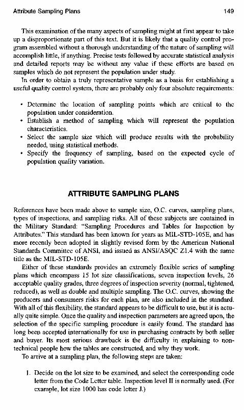
This examination of the many aspects of sampling might at first appear to takeup a disproportionate part of this text. But it is likely that a quality control pro-gram assembled without a thorough understanding of the nature of sampling willaccomplish little, if anything. Precise tests followed by accurate statistical analysisand detailed reports may be without any value if these efforts are based onsamples which do not represent the population under study.
In order to obtain a truly representative sample as a basis for establishing auseful quality control system, there are probably only four absolute requirements:
• Determine the location of sampling points which are critical to thepopulation under consideration.
• Establish a method of sampling which will represent the populationcharacteristics.
• Select the sample size which will produce results with the probabilityneeded, using statistical methods.
• Specify the frequency of sampling, based on the expected cycle ofpopulation quality variation.
ATTRIBUTE SAMPLING PLANS
References have been made above to sample size, O. C. curves, sampling plans,types of inspections, and sampling risks. All of these subjects are contained inthe Military Standard: "Sampling Procedures and Tables for Inspection byAttributes." This standard has been known for years as MIL-STD-105E, and hasmore recently been adopted in slightly revised form by the American NationalStandards Committee of ANSI, and issued as ANSI/ASQC Z 1.4 with the sametitle as the MIL-STD-105E.
Either of these standards provides an extremely flexible series of samplingplans which encompass 15 lot size classifications, seven inspection levels, 26acceptable quality grades, three degrees of inspection severity (normal, tightened,reduced), as well as double and multiple sampling. The O.C. curves, showing theproducers and consumers risks for each plan, are also included in the standard.With all of this flexibility, the standard appears to be difficult to use, but it is actu-ally quite simple. Once the quality and inspection parameters are agreed upon, theselection of the specific sampling procedure is easily found. The standard haslong been accepted internationally for use in purchasing contracts by both sellerand buyer. Its most serious drawback is the difficulty in explaining to non-technical people how the tables are constructed, and why they work.
To arrive at a sampling plan, the following steps are taken:
1. Decide on the lot size to be examined, and select the corresponding codeletter from the Code Letter table. Inspection level II is normally used. (Forexample, lot size 1000 has code letter J.)

2. Find this letter in the single sampling plan master table for normal inspec-tion, and note the corresponding sample size. (For example, Code letter Grequires a sample size 32.)
3. Decide on the acceptable quality level (e.g., let us select 1.5%) and findthe accept/reject level. (For example, for letter Q, and 32 samples, withacceptable quality level 1.5%, the lot of 1000 would be accepted if 1 orless defects were found, and would be rejected if 2 or more rejects werefound.)
Detailed instructions and definitions are found in the first several pages of thestandard, including techniques for special sampling plans.
It is suggested that these special plans be avoided, or used with great care.They were probably introduced to limit the costs of testing when either the testitself was costly or time consuming, or when destructive testing of several expen-sive products was prohibitive. (For example, destructive testing of an engine, aparachute, or complex electronic assemblies.) For most food products, these arenot particularly important considerations. There is a psychological approach todouble sampling plans: they erroneously seem to present a "second chance" to thetesting of the acceptability of a lot. (If it fails on the first test, draw additionalsamples.) To the statistically informed, this is nonsense. The multiple samplingplans become quite complex in their usage, and there is a tendency for theuninformed to attempt to use short cuts, which makes the results meaningless.
With these precautions in mind, the standard provides a useful attribute sam-pling plan for industry. In the introductory remarks, it suggests several inspectionapplications: end items, components and raw materials, operations or services,materials in process, supplies in storage, maintenance operations, data or records,and administrative procedures. The user is cautioned to consult the O.C. curvescontained in the standard to find a plan which yields the desired protection (risk).
6 Test Methods
An attempt to cover the subject of test methodology in a single chapter would beclose to impossible. There are hundreds of books describing thousands of testmethods for a myriad of food products and their components. What we should beable to accomplish is a brief discussion of some of the relationships between testmethods and quality control, along with a bibliography for guidance.
Selection of tests might be classified in three groups, those that provideinformation relative to:
• legal requirements• process, product, packaging specifications• special guides.
Legal requirements may be found for nearly every product: net contents, micro-biological purity, nutritional claims, absence or presence of food components or ofnon-food components. The following are a few FDA requirements selected at ran-dom from the Code of Federal Regulations. If vitamin A is added to milk, eachquart must contain not less than 2000 International Units. Egg rolls must containover 2.56% by weight of whole egg solids. Each part of the contents of a packageof margarine must bear the word "margarine" in type or lettering not smaller than20-point type. Ninety-nine percent disodium ethylenediaminetetraacetate may beused up to 500 parts per million to promote color retention in canned strawberrypie filling. When processing bottled drinking water, cleaning and sanitizingsolutions used by the plant shall be sampled and tested by the plant as often asis necessary to assure adequate performance in the cleaning and sanitizing opera-tions. In these few examples, there is no question as to the tests to be conducted.Certainly, the first step in selecting tests is to find the legal requirements at alllevels of government. Some city or state codes exceed the requirements of thefederal laws.
When selecting test procedures not legally prescribed for controlling thequality of a process, product or package, methods used may be rigorously

standardized, or they may be developed in-house along scientific but lessstringent techniques. There are also many arbitrary methods which are developedin-house which are not recognized by industry or government, but which servea specific purpose in controlling quality. The most important test of all is theuser test. If a product meets all of the known legal requirements and companyspecifications, but doesn't work, the company is in serious trouble. Obviously, thespecifications are incomplete. A painful example happened in a company whohad successfully manufactured tea bags for years. The bag specifications appearedto be complete: bag dimensions, 35 grains of product per bag, 3 in. string length,in 4 in. square tag, uniform seam width, seal complete on three sides, etc. Suddenly,an unexpected torrent of consumer complaints poured in, all describing the stringtearing loose from the bag. The problem was traced to insufficient wet strength ina shipment of tea bag paper—for which there was no specification. The qualitylaboratory test was scientifically designed to evaluate all of the dimensionslisted above, plus a "final product test" in the cup. Unfortunately, the scientifictest did not include lifting the brewed tea bag from the cup by its string. Theproblem would have been revealed the day the first roll of defective paper wasreceived, if only the lab had duplicated the consumer's method of preparing a cupof tea.
Selecting the formal test methods for legal requirements is usually not aproblem, since the requirements generally refer to clear test requirements.
To set up a library for test methods, several books are clearly needed. A list ofthe most useful follows:
Standard Methods for the Examination of Water and Wastewater. American Public HealthAssociation.
Bacteriological Analytical Manual. Food and Drug Administration.Gruenwedel, D. and J. Whitaker. Food Analysis. ISBN 0-8247-7181-8. Dekker.Harrigan, W. Laboratory Methods in Food and Dairy Microbiology. ISBN 0-12-326040-X.
Academic Press.Joslyn, M. Methods in Food Analysis. Academic Press.Microscopic Analytical Methods in Food and Drug Control. Food and Drug
Administration.National Research Council. Food Chemicals Codex. ISBN 0-209-02090-0.National Academy Press.Pomeranz, Y. and C. Meloan. Food Analysis Theory and Practice. ISBN 0-442-28316-4.
Van Nostrand Reinhold.Richardson, G. Standard Methods for the Examination of Dairy Products. American
Public Health Association.Speck, M. Compendium of Methods for the Microbiological Examination of Foods. ISBN
0-87553-117-2. American Public Health Association.Training Manual for Analytical Entomology in the Food Industry. Food and Drug
Administration.Williams, S. Official Methods of Analysis. ISBN 0-935584-24-2. Association of Official
Analytical Chemists.Zweig, G. and J. Sherman. Analytical Methods (12 Volumes) ISBN 0-12-784312-4.
Academic Press.

Of course, many of these references will not be applicable to all food products, butit might be well to review each for possible adoption of modified test methods.The next list contains references fairly commonly used by the food industry, andare arranged by type of test.
GENERAL ANALYSIS
Aurand, L. et al. Food Composition and Analysis. Van Nostrand Reinhold.Birch, G. Analysis of Food Carbohydrate. ISBN 0-85334-354-3. Elsevier.Chaplin, M. and J. Kennedy. Carbohydrate Analysis: A Practical Approach. ISBN
0-947946-68-3. Oxford.Fennema, O. Food Chemistry. ISBN 0-8247-7271-7. Dekker.Fresenius, W. Water Analysis. ISBN 0-387-17723-X. Berlin.Gilbert, J. Analysis of Food Contaminants. ISBN 0-85334-255-5. Elsevier.Kurtz, O. Micro-Analytical Methods for Food Sanitation Control. Association of Official
Agricultural Chemists.
SPECIAL INSTRUMENTATION
Gilbert, J. Applications of Mass Spectrometry in Food Science. ISBN 1-85166-801-X.Elsevier.
Lawrence, J. Food Constituents and Food Residues: Chromatographic Determination.ISBN 0-8247-7076-5. Dekker.
MacLeod, A. Instrumental Methods of Food Analysis (1973). Halstead.
MICROBIOLOGY
Recommended Methods for the Microbiological Examination of Foods. American PublicHealth Association.
Beuchat, L. Food and Beverage Mycology. ISBN 0-442-21084-1. Van Nostrand Reinhold.Corry, J. et al. Isolation and Identification Methods for Food Poisoning Organisms.
ISBN 0-12-189950-0. Society for Applied Bacteriology.Post, F. Laboratory Manual for Food Microbiology. Star.Sharpe, A. Membrane Filter Food Microbiology. ISBN 0-86380-065-3. Wiley.
SENSORY
Bourne, M. Food Texture and Viscosity: Concept and Measurement. ISBN 0-12-119060-9.Academic.
Moskowitz, H. Food Texture: Instrumental and Sensory Measurement. ISBN 0-8247-7585-6.Dekker.
O'Mahoney, M. Sensory Evaluation of Foods: Statistical Methods and Practices.ISBN 0-85334-272-5. Elsevier.
Piggott, J. Sensory Analysis of Foods. ISBN 0-85334-272-5. Elsevier.

Next, a list of fairly recent books covering many aspects of test methods follows.
Aurand, L. and A. Woods. Food Composition and Analysis. ISBN 0-442-20816-2.Van Nostrand Reinhold.
Banwart, G. Basic Food Microbiology. ISBN 0-87055-322-4. AVI.Charalambous, G. Analysis of Food and Beverages. ISBN 0-12-16916-8. Academic.DiLiello, L. Methods in Food and Dairy Microbiology. ISBN 0-87055-411-5. AVI.Gorman, J. Principles of Food Analysis for Filth, Decomposition and Foreign Matter. Food
and Drug Administration.Harrigan, W. and M. McLance. Laboratory Methods in Food and Dairy Microbiology.
ISBN 0-12-326040-X. Academic.Jay, J. Modern Food Microbiology. ISBN 0-442-24445-2. Van Nostrand Reinhold.Jellinek, G. Sensory Evaluation of Food. ISBN 0-89573-401-X. VCH Pubs.Jowitt, R. Physical Properties of Food. ISBN 0-85334-213-X. Elsevier.King, A. Methods for Mycological Examination of Food. ISBN 0-306-424479-7. Plenum.Knorr. Food Biotechnology. ISBN 0-82477578-3. Dekker.Lee, F. Basic Food Chemistry. ISBN 0-87055-4. AVI.Macral, R. HPLC in Food Analysis. ISBN 0-12-46780-4. Academic.Morris, B. and M. Clifford. Immunoassays in Food Analysis. ISBN 0-85334-321-7.
Elsevier.Moskowitz, H. Applied Sensory Analysis of Foods. ISBN 0-8493-6705-0. CRC.Mountney, G. Practical Food Microbiological Technique. ISBN 0-442-22688-8. Van
Nostrand Reinhold.Okus, M. Physical and Chemical Properties of Food. ISBN 0-916150-82-8. American
Society of Agricultural Engineering.Osborne, B. and T. Fearn. Near IR Spectrographic Food Analysis. ISBN 0-470-2675-6.
Wiley.Post, F. Laboratory for Food Microbiology and Bacteriology. ISBN 0-89863-127-0. Star.Rockland, L. and G. Stewart. Water Activity. ISBN 0-12-591-350-8. Academic.Stewart, K. and J. Whitaker. Modern Methods of Food Analysis. ISBN 0-8705 5-462-X. AVI.Vaughn, J. Food Microscopy. ISBN 0-12-715350-0. Academic.
Finally, we present a short list of industry methods. By contacting suppliers, itis possible to obtain other industry test methods which have been developed byprivate industry and by trade associations.
Evaluating a Double Seam. Dewey and Almy Chemical Co., Divn. W. R. GraceCo., Cambridge, MA.FPA Technical Manual of Specifications and Test Procedures. Published by the National
Flexible Packaging Association, Cleveland, Ohio.Index of CCTI Recommended Industry Standards and Testing Procedures. Published by
The Composite Can and Tube Institute, Washington, DC.Official Microbiological Methods of the American Spice Trade Association. Published by
the ASTA, Englewood Cliffs, NJ.Specifications and Methods of Analysis. N. V Cacaofabriek De Zaan, Holland.
Hundreds of test methods developed specifically for food analysis are availablefrom instrument manufacturers. When contemplating additions to laboratory

equipment, check with the manufacturer's technical department to obtain lists ofapplications. Contact the manufacturer of presently owned equipment for newapplications developed since the original purchase. Although all of these industrytests may not be accepted as official analytical methods, they may provide usefulrapid analyses on such equipment as infrared analyzers, HPLC, ultravioletand visible spectrophotometers, mass spectrophotometers, ion chromatographs,polarographs, and others.
7 ProductSpecifications
Assembling specifications to describe a product would seem to be the simplestpart of a quality control program. A bread bakery might decide to develop a caketo round out the product line. Once the kind of cake has been decided, a brain-storming session with the bakery staff can produce a list of attributes which needto be defined. Consider Figure 7-1. In order to convert the attributes listed intospecifications, there are three basic questions to be answered:
• What do you want to make?• What are you capable of making?• How much can you afford to spend?
Converting descriptive quality terms into concrete specification numbers canbe accomplished logically by the use of statistical tools. A statistical evaluationof process capability will define the limitations of cakes which the plant can con-sider manufacturing. Capability studies will also lead to decisions regarding thenumerical values to be applied to each of the variables under consideration: theweight, moisture, height, color, acidity, shelf life, and cost. The range of attrib-utes can be determined by the formulation of experimental designs, and analysisof the results: texture, grain, rigidity, sweetness, flavor, etc. Compromises regard-ing shelf life, packaging, ingredients, dimensions, and product characteristicssuggested by the experiments can then be effected through discussions withmarketing, accounting, distribution, engineering, production, and other depart-ments. Finally, the specifications can be presented to management for approval.
Now that the cake and frosting specifications are spelled out, the details of theingredients, packaging, processing and storage must also be specified in order tobake and market cakes with the consistent quality level required. Although thesespecifications usually require fewer department meetings, using the same statis-tical design and analysis of experiments is the surest path to reliable data.
If any of the above steps to converting an idea into a product specification isomitted, disappointment on the production floor and in the marketplace becomes

Diameter
Height
CAKE SLICE FROSTING GENERAL
COLORAROMA
TEXTUREFLAVORACIDITYMOISTNESSGRAIN
CRUMBSPLIT
STRENGTHRIGIDITY
THICKNESSCOLORGRAIN
CHEWINESSGREASINESSFLAVOR
SWEETNESS
WEIGHTINGREDIENTSPACKAGINGSHELF LIFE
SHIPPING STABILITYSTERILITYDIMENSIONS
Figure 7-1. Quality attributes of a frosted cake.
likely. If specifications are either overlooked or unrealistic, quality failure onthe production floor is bound to cause high scrap and rework costs; and qualityfailure in the marketplace is bound to cause loss of sales.
Listing the specification data for an existing product is a simpler task thanwriting specifications for raw materials or ingredients produced by others. Theselection of the ingredients from the vast maze of materials available in the mar-ketplace can appear overwhelming. Is it possible to select and then specify aningredient which has performance, flavor, uniformity, price, stability, and puritycharacteristics which will in turn provide specific performance, flavor, uniformity,price, stability, and purity characteristics to the finished product? And assuming thatsuch a selection exists, is it then possible to assign to that ingredient the requiredspecification data which the suppliers can meet consistently? The answer to bothquestions is "yes." For the sake of expediency, it may be practical to establishgreatly simplified and fairly broad specifications at the outset, but by the contin-ued use of a program of statistical experimental design and analysis, the specifi-cations can be fine-tuned to assure uniform quality.
The techniques of experimental design and analysis, process capability study,and sensory testing will be discussed later. For the present, let us examine the con-tent of specifications. To start with, an ingredient specification for cocoa is pre-sented in Figure 7-2. The numbers shown are illustrative only, and represent valueswhich might be required for a frosting mix ingredient. In order to arrive at a spec-ification shown in Figure 7-2, the Boston Biscuit Bakery will have completed sev-eral series of tests in which each of the data listed was found to be required for thequality cake desired, or were required by various laws and regulations. Much of theinformation is available from cocoa manufacturers, but not all of the availableanalyses are required in the ingredient specification. For example, compositiondata is available for 14 chemical elements, 7 vitamins, oxalic acid, theobromine,starch, sugars, sulfates, and organic acids all of which may be found routinely incocoa products. There is no point in listing this data in the specification merely

BOSTON BISCUIT BAKERY
Chocolate Cake #CC071 Ingredient Specification
INGREDIENT: Cocoa powder#FCP 071
DATE APPROVED: Sept. 20, 19-
APPROVED SUPPLIERS:Andrus Cocoa Co. Supl#C3Filbert Specialties Supl#C1APPROVED BY: ACG
DESCRIPTION: Medium fat cocoa, conforming to the standard of identity asdescribed in 21 CFR 163.112 and 163.113, and produced in accordance with GoodManufacturing Practices detailed in 21 CFR Part 118, Cacao Products. GrasClearance 21 CFR 182.1.
ATTRIBUTE
PHYSICAL:
CHEMICAL:
Color
FlavorFineness
OdorShell ContentFat ContentLecithinMoisturePHLipase activity
MEASUREMENT
B2-B4
Betw.Std A and Std B99% minimum
Free from off odors5% maximum10.0-12.0%4.0-5.75%5.0% maximum7.0-7.4Negative
TEST METHOD
Agtron A#76Phototron P#3BBB Method #0449Wet, thru 200 Meshsieve (0.075 mm)BBB Method #0006BBB Method #0720AOAC 13.036BBB Method #0724AOAC 13.003AOAC 13.008BBB Method #0726
MICROBIOLOGICAL:Std Plate CountMolds per gYeasts per gEnterobacteriaceaeE. coll per gSalmonellae
5,000 maximum50 maximum50 maximumNegative in 1 gNegativeNegative
FDA/APHABBB Method #0728BBB Method #0729BBB Method #0730FDA/APHAFDA Bacty Manual
PACKAGING:50-pound multiwall paper bags, polyethylene-lined. Each bag labeled withproduct name, manufacturer, production lot.
STORAGE, SHIPPING:Shipped with no more than 2 sublets per delivery. Transported according to21 CFR 1 10.80. Pallets to be stored in cool, dry (R.H. less than 50%) area,isolated from spices and flavorings. Shall comply with storage conditions inaccordance with FDA good manufacturing practices.
SAMPLING PROCEDURE:Samples shall be taken according to BBB Procedures specified in samplingmanual #BBB Manual #4.
Figure 7-2. Cocoa powder specification.

because the figures are available. The specification requirements should be con-cerned only with those variables which might affect the quality of the final product.
Similar specifications are prepared for each ingredient used in the standardizedBBB cake formulation. This insures that the starting conditions for the productmanufacture will be correct. This is the second of the three classes of specifica-tions required for a quality control system. In addition to the ingredient specifica-tions and the finished product specification discussed above, the need for aprocess specification should be obvious.
Process specifications are proprietary, and are usually in a continuous processof evolution as new machinery, new raw ingredients, new process tests, and newformulations are discovered. In the case of the BBB cake, process controls areevolved for each of the unit operations:
• Ingredient weighing• Blending• Mixing• Depositing• Baking• Cooling• Packaging.
Process specifications for each operation are developed from process capabil-ity studies, and test methods are improvised as necessary to assist in measuringthe attributes considered critical to the process. As discussed under HAACP, thecontrol points are discovered from analysis of the process steps and their effectson the product. Both the product and the process equipment are included in theprocess specification network. For example, time-temperature relationships dur-ing the baking cycle must be measured and recorded for both the oven equipmentand for the cake itself during the baking cycle.
Process specifications are the most complex of the three types. Even startingwith raw materials which fall within the ingredient specifications, small variationsin the flour composition, coupled with trace variations in the leavening agents andminor differences in atmospheric pressure can combine to upset the normalleavening process and thus create an in-process oddity which cannot be readilycorrected by unbending process controls.
Each industry seems to collect its own group of such oddities. The density of adehydrated food product was found to shift markedly each afternoon, even thoughno known changes in either the ingredients or the process were occurring. Thecause was finally found to be an afternoon wind blowing against the dehydrator airinlet which upset the drying air flow. In a french fried potato plant, the raw pota-toes tested satisfactorily when received, but turned darker than process specifica-tions permitted when processed. It was discovered that rotation of stock was notbeing carefully followed and, as a result, some of the raw potatoes had started toincrease their sugar content in storage, thus frying darker. Another mystery wentunexplained for years in a tea packaging operation where, periodically, packageswould appear with unusually high (and undesirable) dust content.

This portion of the process specification may read more like a recipe than aprocess control. Subsequent data concerned with air flows, purge times, temper-atures, oven speeds, and interactions of these variables with the product variablesare often more descriptive. Since moisture content of the cake is a critical vari-able, a process specification would have to include a table of expected values ofmoisture levels for various combinations of oven conveyor speed and tempera-tures in both primary and secondary sections of the oven. Similarly, a processspecification covering the cooling cycle would need to list either the cooling timeor the cooling conveyor speeds at various ambient temperatures in order to pro-vide uniform product quality.
To summarize this discussion of specifications:
1. Start with a description of the ideal product.2. Through studies of available ingredients and process experimentation,
define attainable product specifications.3. Prepare optimum ingredient specifications.4. Prepare optimum process specifications.
All ingredients were within specification, and all process controls werewithin specification; yet, the problem persisted. Ultimately it was discovered thatdust was accumulating in the ends of a lengthy feed hopper above the scales, andthen abruptly emptying into the production line packages. It is this type ofexceptional line or product performance which makes process specifications sodifficult to compile.
BOSTON BISCUIT BAKERY
Chocolate Cake #CC071 Process Specification
DATE APPROVED: Sept. 20, 19-
INGREDIENTWEIGHING
Small Ingredients
Butter flavor B03Albumen powderVanillinSaItREFI 7 S
APPROVED BY: ACG
Scale #S2007 Precision 0.25 ounce
3lbs74
120
7.75 oz8.004.252.00
Mix 4.5 minutes on Ingredient Blendor #BI02. Temperature 65-80 deg.
Sodium tartrate ST04Calcium phosphate CP04
52
0.000.25
Add to Ingredient Blendor #BI02. Blend 1 .75 minutes. Maximum 90 deg.
Store in sealed drums at 65-90 deg. for no more than 8 hours.
Major Ingredients etc. etc.

8 Process Capability
Before examining the mechanics of process capability analysis, it would be wiseto define the subject. With only two words to define, this would appear to be atrivial task. According to the dictionary, "process" refers to steps (or operations,or changes) leading to a particular result. "Capability" is defined as the capacityfor an indicated use. Let us explore a few of the definitions proposed by variousauthorities in the field.
"Process capability is the measured, inherent reproducibility of productionturned out by a process."
Juran, Quality Control Handbook
"The minimum spread of a specific measurement variation which will include99.7% of the measurements from a given process."
B. Hansen, Quality Control Theory and Applications
"The minimum range of values of the process output variable which includesat least 99% of the observations under normal operating conditions."
D. Braverman, Fundamentals of Statistical Quality Control
"Process capability is quality-performance capability of the process with givenfactors under normal, in-control conditions."
A. Fiegenbaum, Total Quality Control, Engineering and Management
"Process Capability—the level of uniformity of product which a process iscapable of yielding."
DataMyte Corporation, DataMyte Handbook
"Process capability is determined by the total variation that comes from com-mon causes—the minimum variation that can be achieved after all specialcauses have been eliminated."

W. Edwards Deming, "On some statistical aids toward economic production,"Interfaces, Vol. 5 No. 4, August 1975. The Institute of ManagementSciences, Providence, Rhode Island
No two of these definitions are in complete agreement. Nor do they clarifywhether we are concerned with a complete product, a single step in the process,a vendor's product quality (raw material), or if a machine can be considered to bea "process." One definition refers to the "spread of a measurement;" another, the"reproducibility of production;" a third, "range of values," and "quality perform-ance," "99.7% of the measurements;" "minimum variation," etc. Perhaps thesimplest definition above is the most useful: "the level of uniformity of productwhich a process is capable of yielding." We shall start working with this one.
Note that this definition does not concern itself with how well the process iscurrently working, but aims at what the process is capable of yielding. The impli-cation here is that at times the process works more uniformly than at other times,and more important, there is a possibility that the process might be furtherimproved. Herein lies the value of process capability studies: they will establishthe best quality the process is currently capable of producing so that realisticcontrol limits and specifications can be drawn up. That's the immediate goal. Inaddition, the studies required for capability analysis will also suggest areas wheremodifications might be looked at for further improvement.
Deming refers to variability in manufacturing processes as consisting of twotypes: common and assignable. The common causes are those which are inherentin the process, remaining there until management sees fit to change theprocess to modify or eliminate them. Assignable causes are external factors whichcan be eliminated or controlled, and although they affect the process, are not a partof it. Examples of assignable causes are incorrect packaging material, improperidentification of raw material, wrong laboratory data. Examples of commoncauses: poor lighting, gradual machine wear, inadequately trained operator, inex-act measuring equipment. Process capability studies are conducted on processes"which have all assignable causes eliminated, and insofar as possible, have allcommon causes reduced to a minimum. By definition, these conditions existwhen a process is in statistical control. Herein lies the problem: more often thannot, a process capability study is required for new or proposed processes whichhave not had an opportunity to be freed from as yet unidentified assignablecauses. This might explain why there are definition conflicts. Different qualitycontrol practioners have conducted process capability tests under unique condi-tions for which they have later evolved a definition which suited their purpose.
Having cleared the air of that semantic problem, let us examine a simplifiedexample of a process capability study. The example is taken from a plant process-ing melba toast. One of the quality criteria is the color development in the finalstages of oven browning. Individual pieces of toast are scanned by a spectropho-tometer which has been calibrated to reflect yellow-brown light over a reducedspectrum. The readout is expressed in percent of a standard yellow-brown refer-ence plate, and a value of 41 is considered to be optimal. Data is collected every30 min starting at early morning and continuing over 15 hr. The results are

tabulated and graphed as shown in Table 8-1 and Figures 8-1-8-3. Superimposedon the graph are the calculated values for the average and for the upper and lowerthree-sigma control limits (UCL and LCL). These limits are considered to betotally unsatisfactory; the upper limit is far too light, and the product tested at thelower limit is nearly burned. There are many variables at play over these 15hrswhich contribute to this unsatisfactory range.
Table 8-1. Example of Process Color Capability Data
Sample no.
123456789
101112131415161718192021222324252627282930
AverageStandard deviation3 x Standard deviation
Control Limits
Color unitsevery 30 min
344562354433425044533332574540334520443159345229454452333429
41.1
10.0
30.11 1 .0-71 .2
Color unitsconsecutive
424441444543444441413839404141404340443839404442454244434742
42.02.236.7
35.3-48.7
Color unitsimproved proc
414141424145424341403938394041414241424241404040414241414241
41.0
1.29
3.8
37.2-44.8

Figure 8-3. Color units consecutive, improved process.
Sample Number
Figure 8-2. Color units consecutive.
Sample Number
Figure 8-1. Color units every 30 min.
Minutes
UCL
AVG
LJCL
UCL
AVG
LCL
UCL
AVGLCL

To limit the variables, another set of data is obtained in which the samples aretaken continuously, 15 seconds apart, until 30 samples have been obtained. Theseare then examined, data recorded and graphed, and control limits applied as above(see Figure 8-2). Now we find control limits within 6.7 units of the average value of42.0. Contrast this with the range of 30 units in either direction of the averageobserved in the 15-hr sampling period above. What we have discovered is thecapability limits of the process when most of the variables are unchanging. Tophrase this simply: the process under the best conditions now available willprocess toast with a range of 13.4 color units.
During the course of the study thus far, certain observations of the process mayhave been questioned with the possibility of reducing the variability. For example,it may have been observed that the widest swings in data over the 15-hr testperiod were the result of the coarse control setting on the trim burners. That is,the sensitivity to temperature control was set at the lowest range, causing theburners to alternately surge and then coast. This resulted in marked differences inthe product color units. Let us further suppose that the range setting on the burnerwas moved up a notch so that the burners cycled more often as the temperaturestarted to drift. With this improved process control, it was decided to take anotherset of data, (see last column Table 8-1 and Figure 8-3) as shown on the accompa-nying table under "improved process."
Here we find that the consecutive sample series obtained showed a reduced vari-ability, and an improved process capability: control range reduced to 7.8 color units.
This example demonstrates how a process capability study may be made usingsimple statistical control charts. It also demonstrates how process improvementsmay be discovered, implemented, and verified.
Again, it should be emphasized that the above example is simplified. In thereal world, there are at least three major changes to be considered:
1. 30 samples are not enough. Generally, at least 100 samples will be requiredto obtain a reasonable estimate of population mean and standard deviation.
2. Subgroup size of one is more difficult to calculate than larger sizes.Subgroups of three or five may be used, thus permitting use of tables toestimate standard deviation. Bear in mind that there we are dealing withmeans, not individuals, and the results should be interpreted with constantreference to the means.
3. After conducting the first series of determinations to establish process capa-bility, there is rarely an opportunity to immediately run process improve-ment tests as shown in the example. These require time to plan adequately.
A word of caution regarding the second paragraph above. Not all qualitycontrol practitioners would agree that there is justification in labeling the controllimits for means as synonymous with process capability. But there is certainlya practical use for determining means control limits to explore, at least initially,the capabilities of a process. Eventually, it may be necessary to measure the vari-ability and control limits of individual products. After all, the customer examines the

product purchased, not a subgroup of products. In fact, the customer doesn't carewhat the average quality is—only the quality of the individual product purchased.This is not necessarily true for intermediate products, however. In a corn cannery,there is no need to know ear-to-ear variability; bushel-to-bushel quality data mayreadily suffice.
A more complete determination of process capability may be arrived at byinvestigating the time-to-time variability of the process. The "consecutive" data areperfectly valid, but they define the best possible control limits of the process as itpresently operates. It would add to the value of these data if some measurement ofprocess shift could also be measured. An examination of the data in the "every 30min" graph shows no particular drift pattern, but clearly indicates that the processdoes not meet the control limits determined in the "consecutive" process capabil-ity study. Specifically, if the capability control limits of 35.3-48.7 were appliedto the "every 30 min" data, 11 points would be out-of-control on the low side, and7 points would be out-of-control on the high side. That means a total of 18 of the30 points are out-of-control. This process is obviously in need of attention.
By contrast, the "consecutive" data show a rather tightly controlled processover the period of time required to obtain the data. Somewhere between that periodand 30 min, the process has drifted several times. To locate that interval, it willbe necessary to conduct a detailed test in which samples are taken at fairly shortintervals for a total time of 30 min. To simplify calculations, it is suggested that theaverage color units of every five samples (in order of production) be plotted on agraph. A visual examination of the graph should reveal the interval of time duringwhich the process is stable, and the approximate time after which the process tendsto drift in one direction or another. Once this interval has been uncovered, the causesfor drift can be studied so as to reduce variability. Without taking this step todetermine the minimum drift interval, attempts at process improvement testing arelikely to be disorganized, random, and frequently fruitless.
An example of a graph showing process drift is shown in Figure 8-4.
Color Units
Sample Number
DriftDrift
Drift Drift
Drift
Drift
Drift
7 min
Figure 8-4. Average of five successive samples taken at 12 s intervals.
It appears that the shortest interval between a stabilized process and thestart of a drift is about 7 min. Therefore, the process should be evaluated every7 min and adjustments made if required. If, in the case of melba toast processing,the key to the color unit drift is found to be oven temperature, then the evalu-ation and correction should be made by a temperature sensor and controllerif available; in a manual process the evaluation would be performed by an opera-tor who would be instructed to adjust the oven temperature if the reading is out-side of the process control limits. If the key to color drift is found to be ovenconveyor speed, then this would be the factor to be adjusted to maintain processcontrol.
A number of sampling and adjusting schemes can be devised, depending uponthe process, the equipment, and the operators. For example, it would be possibleto establish a 14- min evaluation cycle, with the understanding that if the processdrifts out of limits, as much as 7 min of production might be out of the colorcontrol limits.
Note that the process control limits determine the obtainable uniformityof product. In some instances, this might be far more uniform than is requiredby the customer. In such a fortunate situation, the process need not beadjusted until the specification limit is reached, possibly reducing the cost ofproduction.
As we have already seen, there are many uses to which process capabilitystudies can be applied. Here are some others:
1. Process selection. When several processes are under consideration,capability analysis will assist in selection of the most effective one.
2. Tolerance compliance. Process capability analysis (PCA) will predict theextent to which the process is capable of holding.
3. Machine selection. PCA can be used to assign machines to the classes ofwork for which they are most suited.
4. Selection and training of inspectors. When a PCA has been prepared, thecontrol limits provide reliable benchmarks to evaluate inspectors' abilityto adequately measure quality.
5. Identification of troublesome steps. In a series of sequential pro-cessing steps, PCA of each step may identify the one responsible forquality abnormalities. This reduces the research necessary to find asolution.
6. Research criteria. Theories of defect causes may be readily evaluated byPCA during quality improvement programs.
7. Audit tool. A series of PCAs performed on the same process will oftendisclose the frequency of process reviews required to insure adequatemaintenance, inspector instruction, operator performance, personnelsupervision, analytical instrument calibration, etc.
8. Setting specifications. If the product is to succeed, its quality specifica-tions must lie beyond the process capability limits.

CAPABILITY INDEX
One of the end products of a process capability study is the control chart show-ing the upper and lower control limits of a controlled process. The control limitscover a range of six-sigma. Another end product is the capability index. Thecapability index compares the product specification range with the six-sigmarange. The index may be useful to those who prefer to express test results innumbers, rather than in words. It may also find value where a company hasa vast number of specifications and is constantly in need of comparing processcapabilities with control limits.
The calculations are simple:
Process capability index = Cp
Allowable process spreadCapability index = —-
Actual process spread
_ Specification limitsProcess control limits
_ USL - LSL~ UCL - LCL
_ Tolerance" 6a
All of these equations say the same thing: subtract the lower specification limitfrom the upper specification limit, and divide the result by the difference betweenthe upper and lower control limits (or six standard deviations). The number foundby this simple calculation determines whether or not the process is capable ofmeeting the specifications.
If the specification spread is the same as six-sigma (Cp =1), then approxi-mately 0.3% of the production can be expected to be out of limits. If six-sigma isless than 75% of the specification spread, then the process is generally consideredacceptable and capable. (That is, Cp = 4/3 = 1.33.) In tabular form:
Capability index
1 .33 or greater1 .00 to 1 .33
1 .00 or less
Conclusion
Process is satisfactoryProcess is capable, but marginally as the index
approaches 1 .00Process is unsatisfactory

ExampleLet us assume the specification for a food product limits the ferric iron content between14 and 22 parts per million. A process capability study shows control limits at:
LCL = 15 ppm; UCL = 21 ppm.Cp = (22-14)7(21-15)
= 8/6=1.33
Therefore, this process is capable of meeting the specification. A control chart illustratingthis example is shown in Figure 8-5.
ppm ppm Ferric IronUpper Spec
-UCL
Average
Lower SpecLCL
Process Capability Index = (22-14)7(21-15)
Process Capability Index = 1.33
Sample Number
Figure 8-5. Control chart—ferric iron content (in ppm).
Figure 8-6. A capable process.
LoverSpecification
Limit
LoverControl Limit
UpperControl Limit
UpperSpecification
Limit

To review: if a process is in control, and if all of the measurements of that processwhich lie between the lower control limit (three standard deviations below theaverage) and the upper control limit (three standard deviations above the average)also lie between the lower and upper specification limits, then the process may beconsidered "capable." An illustration of this is shown in Figure 8-6.
A method to avoid calculating the standard deviation of individuals data:Calculate the average range ( R ) of differences of each successive pair of datapoints, and find the control limits for individuals using the following formulas:
UCL =X + 2.66R
UCL = X - 2.66R
A short cut to finding the standard deviation for individuals when a previous-ly calculated control chart for averages is available: multiply the UCL and LCLby the square root of n, where n is the sample size used in the control chart foraverages. The square root of n converts average data to individual data. Theseindividual control limits may now be used to calculate the capability index usingthe above formulas.
The capability index discussion above refers to 6cr as the area between theupper and lower control limits. This should not be confused with the 6a qualityprogram popularized by an electronic manufacturing company. This organizationwas determined to reduce defects to parts per million, rather than the generallyaccepted 3 parts per 1000. In order to accomplish this, they started by placing thespecification limits at 6 standard deviations on either side of the mean, shiftingthe process mean 1.5 standard deviations higher than center, and improving theprocess until the upper process control limit was within the specification limit.(Note carefully the italicized process and control verbiage in this explanation.)Perhaps the following table and discussion will make this more clear.
Research had determined that the process mean normally shifted higher by+ 1.5(J for the company which evolved this quality control system. The unitsout of specification under these conditions would have been expected to rise to6.8 per million; however, it was theorized that since the lower control limit wasalso raised by 1.5<r, there would be zero defects at the lower level, and 1/2 of 6.8or 3.4 defects at the upper level. With this reasoning, the company identified the
Table 8-2. Relationship Between Capability Index and Defects
Capability Index
1.01.331.481.672.0
Specification Limits
±30- or 60-±40- or 80-
±4.50-±50- or 100-±60- or 120-
Units per Million out ofSpecification
2700636.8
0.5700.002

quality program as the Six-Sigma Quality Program, which produced 3.4 defectsper million.
Since the program would be successful only if process improvements could beaccomplished to fit within it, one might suggest other, perhaps simpler ways toaccomplish the same defects per million goal. On the other hand, the numeric goal-oriented system has motivated employees, and positive results have been obtained.
BENCHMARKING
The usual understanding of the benchmarking process is based on finding anexternal goal obtained from the best of industry practices. By investigating andincorporating these best practices into its operations, a company can expect tobetter serve its customers, and improve its processes and profitability. Definitionsof external benchmarking suggest continuously measuring and comparing a com-pany's products and processes with those of industry leaders in similar products orservices, and adopting the best of them with whatever modifications are necessary.
Direct competitors are unlikely to embrace this policy of sharing best practices,depending partly on the market share of each company However, companies withdifferent products or uncommon market niches may both benefit from frankdiscussions of each other's best practices. Other sources of information are tradejournals, the internet, business consultants, market research organizations, busi-ness and professional association meetings and publications, customers, andequipment vendors.
There are many differing benchmarking plans offered in the literature. Ratherthan recommending a single series of steps and rules for conducting a bench-marking program, it might be of greater value to consider some of the manyquestions which must be resolved before starting.
What management level should interview which host management levelHow is the benchmark target selectedHow can host's information be tactfully verifiedShould the first project be a surefire success or a major goalMust contacts be performed with written questionnaires, or verballyDo host's measurements have the same meaningAre personnel qualified to perform, or are consultant's requiredShould informal contacts be made in addition to office visitsMay an undefined goal be used as a starting pointIs a project schedule desirable—or possibleDoes the host's differing corporate culture account for successAre the units of measurement the same for the two companiesWould information sharing violate any lawHow will use of new information be processed in the companyShould benchmarking be conducted by a team or a department
The techniques involved in benchmarking have been formalized by severalcompanies and authors, and they all seem to have a central theme: Plan / Do /

Check / Act (the Deming Cycle.) However, the terminology used in benchmarkingsteps varies: analysis, implementation, integration, measurement, identification,data collection, functional goals, establishment of performance levels, developaction plans, monitor.
Not to be overlooked is a perhaps more valuable approach to benchmarking:internal process and product improvement made possible through examining themost successful principles and techniques which exist in one's own company. Thediscussion of benchmarking has been included in this chapter on process capa-bility for that reason.
Internal benchmarking is an extremely effective tool and is usually welcomedby both production personnel and management, since it represents the best effortsand previous attainable successes found within the company. In essence, it isbased on a simple principle: "we did it before and we can do it again." Perhapsmost companies have repeatedly used a form of this technique without formaliz-ing it with a title.
Although internal benchmarking can be successfully handled by a single engi-neer, production manager, researcher, or department head, it is more likely to besuccessfully implemented if a team is formed from various company operations.The increased success observed may be due in part to the possibility of contribu-tions of more diverse ideas; but since the team includes members whose depart-ments are affected by the final decisions, they would likely be motivated tocontribute willingly and to actively implement the findings.
The principle of internal benchmarking is to select an operation which workedbetter than normal one which exceeded the normally acceptable (and desirable)control limit for quality, cost, sales, personnel requirements, productivity, linechangeover, absenteeism, consumer complaints, mistakes, scrap, productioninterruptions, accidents, billing, specifications (such as color, flavor, weight,dents, leakers, lumps, solubility, flow, granulation, printing) or other. In a well-structured quality control system, this selection process can be as simple as form-ing a team to identify favorable outliers on process control charts, and selectingthe one which appears to have the greatest potential. In its simplest terms, bench-marking now proceeds to find out how the favorable outlier occurred, set up a testto duplicate those conditions, and if successful, change the methods of operationto include the new conditions.
How does internal benchmarking differ from the normal principles of qualitycontrol and process improvement which have been used for years? Not by verymuch. The major change has been the introduction of a formalized structured sys-tem which includes (usually) team members from several departments. Each com-pany can best decide how to structure the benchmarking process so that it will fitin with their culture. Following is a suggested framework for such a structure.
Form a search team to select a project areaEstablish a specific goal and major objectiveSelect a team consisting of members affected by the goalTrain team to follow specific procedures

Brainstorm goal to select specific projectEstablish resources necessary to achieve goalDetermine data collection proceduresGather and analyze existing dataGenerate additional data as requiredRedefine goal and targetPropose improvement plan (PLAN)Educate and train those involved with plan executionImplement plan (DO)Determine effects of implementation (CHECK)Apply corrections or modifications to implementationStandardize procedures, specifications (ACT)Prepare report on findings, action taken and benefitsPublicize successesReview benefits and start a modified or new improvement project
The major advantages of internal over external benchmarking are the avail-ability of readily interpreted data, some of which might be proprietary, and theknowledge that the culture, environment and operations are constant.

9 Process Control
Once the initial investigative procedures have been completed on a process(specifications, capability analysis), control charts can be constructed and evalu-ated continuously to guide in the production of acceptable quality products. Fromthe company's viewpoint, this is the most visible and the most useful functionof the quality control manager. When progressing from capability analysis toproduction quality control, use of single sample measurements of variables isgenerally superseded by subgroups so that control charts for averages and forranges may be constructed. The procedures for establishing and maintaining thesecharts have been described elsewhere. Our concern here is the interpretation ofthe charts.
In order to interpret a chart, it is essential that a number of factors concerningits selection and construction be reviewed. The function of charts used by a long-established company frequently erodes from the original purpose into routineswhich lose considerable impact on the control of quality. Under these conditions,it would not be unusual to expect that the question "why do we sample at this pointin the line?" might be answered with a shrug and the reply "we always have doneit this way." Many things change over time. New equipment is added to the linewhich makes some older measurements less significant; changes in raw productsor packaging materials might not react to obsolete controls; or new methods onthe line which critically affect quality might be overlooked by the existing qualitycontrol procedures. Periodic review of the principles on which the charts wereconstructed will avoid these problems.
Such a review should consider:
1. Training of the people currently involved with preparing the charts.2. Assuring that the process location where the chart is generated is still a
critical control point.3. Determining whether or not this chart has an appreciable bearing on the
customer's needs.

4. Judging the adequacy of the measurement system used from a standpointof calibration for precision and accuracy, and state-of-the-art techniques.
5. Considering the possible need for an updated process capability studyand control point revision, as dictated by either process improvement, orspecification change.
Control charts are a continuous "picture of the process," and when properlyconstructed, provide the means of continuously producing product of uniformquality. When a single point falls outside of the control limits, something is prob-ably wrong. There are two key words in that sentence. "Something" might be themiscalculation or misplotting of the offending point, or the sampling may havebeen improper due to stratification or ignorance, or the data may have been edited.The other key word is "probably," since 0.3% of the observations of a controlledprocess can fall outside of the control limits by chance alone. Because of thesetwo possible situations, a number of ground rules have been established by vari-ous quality control practitioners. Some say that a control chart need not causealarm until two points are out of limits on the same side of the control limit.Others say three. Some will call for action when there seems to be a trend or apattern in the data. And there are systems which call for two standard deviationsas a warning limit. Or seven points all on the same side of the process averageline. There are also some shortsighted (and probably shortlived) companies whichuse as a ground rule: "No matter how many chart dots are out of limits, we are sofar behind in production we will not stop the line for anything short of a fire."
There are special cases where some ground rules might be applied, but it isunlikely that misinterpretation of a control chart will occur if every out-of-limitspoint "were investigated, and if all other combinations of points within the controllimits were ignored. This statement applies equally to Jf-bar, R, p, n, or c charts.One of the greatest sins in attempting to control quality, and one of the majorcontributors to production costs, is attempting to control quality by adjusting ormodifying when the process is already within the control limits.
With the understanding of the italicized statement in the paragraph above,we will shortly examine some of the special cases where peculiar chart patternsmight be handled as exceptions to the rule. But first, there are some general prin-ciples relating to data points which appear outside of the control limits, and abrief discussion of these follows.
Data on variables charts may first exceed the control limits in one of threeways:
1. If the average is out of limits, but the range is not, chances are that thereis a serious problem with the process. When this does occur, chances arethat all of the observations in the subgroup are out of control, or nearly so.
2. If the range is out of limits but the average is not, the process may be onthe verge of developing an oscillation. It can be expected to soon drive theaverage out-of-limits as well. It is likely that individual items are alreadyclose to or outside of the specification limit.

3. If both the average and the range are out of limits, something drastic hasoccurred, and it can be expected to become worse unless immediate actionis taken.
When attribute charts (p, n, or c) exceed control limits, it may be that a sub-stantial quantity of questionable quality products has been produced, and correc-tive action should be swift. If not, then charts become useless scorecards, andreject/rework loads will build up.
When any chart shows a reading below the lower control limit, immediateattention is needed, but frequently this may not require shutting down the line. Infact, exceeding the lower limit may be advantageous: fewer can leaks than per-mitted, lower bacteria count, less than the minimum moisture vapor transfer rate,unusually low bitter flavor characteristic, a total absence of contamination, or zerosediment. These and many other similar variables and attributes may all be verydesirable in the product, but are generally unattainable. When this type of outlierdata occurs, the process obviously may not need to be stopped, but the causes forthe unexpected quality improvement may form the basis for an improved product,and should be explored immediately before they disappear. Once uncovered,permanent changes may be instituted, and new process control limits adopted.
Of course, this might also be true for charts of some variables where exceed-ing the upper control limit may produce a more desirable quality product. Heretoo, the causes should be explored with the goal of product improvement.
CHART PATTERNS
Normal, in Control
The pattern is random and within the control limits (Figure 9-1). No action iseither needed or desirable.
SAMPLENUMBER
Figure 9-1. Normal, in control.
LCL
LICL

Random Cycles
When found in the X-bar chart, the causes may be due to rotation of operators ormachines, merging processes (such as feeding reworked material into the line, oralternating raw material and supplies), changes in environmental conditions(temperature, humidity), or worker fatigue (Figure 9-2). On the range chart, thecauses may be due to inadequate maintenance of equipment, resulting in wear andintermittent operation. On/?-charts, cycles may occur from merging processes asabove. In addition, failure to use the correct sampling plan for the chart in use canproduce cycles.
Trend (Up or Down)
The chart for averages may trend in one direction (see Figure 9-3) as one rawmaterial is used up and another is introduced. Gradual deterioration of equipment,continuous change in the environment, or change in the production rate will also
UCL
LCL
SAMPLE NUMBER
Figure 9-2. Random cycles.
SAMPLE NUMBER
Figure 9-3. Trend (down).
LCL
UCL

produce a trend. A trending range chart may be the result of gradual improvementor deterioration of a worker's skill, a production rate change, or a change in thenumber of components reaching the process. P-charts are similarly affected.
Abnormal Uniformity
All charts may show a reduced scattering of observations (Figure 9-4) when asuperior skilled employee is present, when the process has been changed (inten-tionally or not), when a key step or key ingredient has been omitted, when defect-free raw materials are introduced, when unusually favorable environmentalconditions exist, or when the wrong control limits are used. Nonrandom samplesselected by an overzealous or improperly trained employee can result in uniformresults. Samples tested on a malfunctioning instrument (such as a sticking scale,electronically insensitive meter, worn vibrator, cam, dusty colorimeter lens) orsubjected to chemical or biological tests using outdated reagents may also showabnormally uniform quality. Range charts are particularly sensitive to conditionsleading to abnormal uniformity.
Recurring Cycles
Charts which show cycles may be related to activities which occur at repeatedtimes (days, shifts, hours, break periods) when changes in the process or the envi-ronment occur regularly (Figure 9-5). The changes may be in workers, supervi-sors, inspectors, scheduled maintenance, ambient temperature or humidity,lighting, or production equipment rotation. Nonuniform cycles may be traced tooccasional temporary equipment stoppages for adjustment or repair. These mayproduce new quality levels when restarting. Cycles may occur occasionally onrange charts from these causes, but the X-bar and p charts are more likely touncover cyclical quality problems.
SAMPLE NUMBER
Figure 9-4. Abnormal uniformity.
LCL
UCL

Excessive Variability
When found on the chart for averages, excessive variability most frequently iscaused by overadjustment of a process (Figure 9-6). When an operator adjuststhe pH downwards simply because it has been above the average for a fewreadings, the chances are that the pH will shortly drift below the lower controllimit. Blending production from two or more lines may drive the range chart outof limits. (Drawing samples of pouches for length measurements when producedon blended lines, where one line is at the minimum length and the other is atthe maximum, would be an example.) Malfunctioning equipment and intermittentuse of variable raw material (such as feeding into the line raw material which isof variable quality or nearly out of specification) may produce peaks and valleyson the range chart and the p-chart. A malfunctioning inspection device may alsoproduce apparent wide variations.
Figure 9-6. Excessive variability.
SAMPLE NUMBER
LCL
UCL
Figure 9-5. Recurring cycles.
SAMPLE NUMBER
LCL
UCL

Wild Outliers
When an occasional control chart plot lies far outside the limits with no apparentcause, it is generally the result of a quality testing error (Figure 9-7). The list oferrors include: mathematical calculation, plotting, sample size, sampling proce-dure, testing, sample contamination, etc. Problems associated with the productionline are rare, and generally non-repetitive: an interruption of power or gas supply,a sticking solenoid or chattering relay, or possibly an omitted operation. Samplesremoved from the line and inadvertently returned to the wrong part of the line canalso produce an otherwise unexplained outlier.
High/Low
X-bar and R charts will often show extreme values with few in between when twosources of raw materials are used, one of which is at the upper end of the qualityspecification, and the other at the lower end (Figure 9-8). As the variable supplyreaches the production line, the process swings rapidly from one end to the other,
SAMPLE NUMBER
Figure 9-7. Wild outliers.
UCL
LCL
UCL
LCL
SAMPLE NUMBER
Figure 9-8. High/low.

rarely pausing in the center. Since product defects would tend to average out,/?-charts might not be affected by two source materials. However, nonrandom sam-ple selection could show high/low p-chart values. The blending of product fromtwo dissimilar lines or from two operators with varying techniques may be respon-sible for this unusual chart. The output of "twin-pack" packaging machines mayproduce units which are within the control limits, but at opposite ends. Dependingon which side of the machine the sample is taken from, variables such as gas con-tent, fill weight, package dimensions, dust content, seal strength and registrationmay appear at either end of the control chart, but rarely in the middle.
The above explanations for patterns in control charts are necessarily incomplete.Considerable detective work is required for explanations for most out-of-limitsdata. Most of the answers are found on the production floor (or at the raw mate-rials supplier plant), and as the relationship between quality control personnel andoperating personnel grows closer, the answers and solutions to production qualityproblems are found more readily. Sometimes the causes are strange and require agreat deal of ingenuity to uncover: vibrations from the freight elevator upsettingthe line checkweighers, burnt paper ashes strewn over the oven contents duringthe Kosher blessing, static buildup during thunderstorms causing blocking ofplastic films on sealers, conscientious line inspectors who want the record to lookgood for the company by eliminating out-of-limits data, afternoon wind imping-ing on air-intake filters and upsetting airflows in dehydrators.
USINGTHE CONTROL CHART ASA QUALITY MANAGEMENTTOOL
What does one do with the charts at the end of the shift—or day, or longer?Some benefit can be found in posting the charts on the production floor as they areprepared so that the operators can see how well they are accomplishing their tasks.A continuing interest is unlikely unless some kind of attention-getting technique isincluded: perhaps posting the name of an outstanding operator for the week; orpreparing a score card comparing shifts (can be risky), or comparing the currentmonth with the same month last year, or displaying a "thermometer of accom-plishment." All of these ideas tend to lose effectiveness because of overexposure.Some are difficult to turn off after they have served their purpose, since a fewemployees remain attached to them. These plans should be considered carefullybefore obtaining approval of management since competitions can cause jealousy,animosity, or even dishonesty if improperly administered. However, the properuse of a carefully planned motivational quality tool is recommended if it is usedinfrequently and has a worthwhile message.
At one time or another, copies of control charts should be sent to everyone inthe company who is even remotely concerned with product quality. Subsequentcopies should not follow unless requested. If few requests are made, a way mustbe discovered to make the charts more colorful, more informative, and more

interesting; then they should be sent out again. Notes and comments should beincluded showing solved problems, quality improvements, productivity gains, andcost reductions. Most important, credit should be shared (deserved or not) withproduction, engineering, accounting, purchasing and marketing departmentswhenever even remotely possible. Suggestions should be solicited.
For those few managers who do ask for daily charts, their interest should berewarded with brief summaries, weekly and monthly reports and short notes aboutother industrys' quality problems and solutions. Charts should be informative, andthey should be "spiced" and embellished with cartoons, or photographs of qualityimprovements, so that the recipients actually look forward to the next issue. As anadditional courtesy, provide managers with informal tours of the production floorwhere they can watch a chart being constructed.
We have left the most important point for last: how does one actually use thesecharts to control quality effectively; that is, what physical steps do quality controlpersonnel take to make the charts work? When an observation exceeds the controllimits, the line should immediately be stopped, if permitted by management, andall production since the previous observation must be set aside and clearly labeledwith a "HOLD" or "NOT TO BE SHIPPED" or "REWORK" tag. Once the cause for the out-of-limits condition has been identified and corrected, the line may be permitted tostart up again, and paperwork is completed for isolating the defective material andproviding instructions for its disposition.
The alert reader might have noticed "if permitted by management" in the para-graph above. For many, this may be difficult to understand, but there are compa-nies which permit only production supervisors to stop production lines. It is stillpossible to operate a quality control system effectively under these conditions, forit is unlikely that any management would also forbid the quality control depart-ment from isolating and holding any defect, whether it be raw material or finishedproduct. Consequently, the out-of-limits material can be isolated at the end ofthe production line, and then held for corrective action. This can be continuedby quality control until the production department realizes that all productionis headed for the rework or scrap area, and will continue to be until the line isstopped and the offending condition corrected. Needless to say, one or two suchexperiences will lead to a revision in management philosophy, and quality controlpersonnel will eventually be authorized to stop defective production.
This procedure of eliminating out-of-limits materials as they are uncoveredin the process by active use of control charts and immediate corrective action isat the heart of quality control, and is the means to reducing defect production,reducing scrap, increasing productivity, and—perhaps most important—reducingcosts. Some quality leaders seem to wish to label this procedure as a newly dis-covered principle of quality control, and insist on providing it with a label: "statis-tical process control," or "zero defects production," or "process quality assurance,"or other. So be it! Regardless of the title given to this procedure, it works well, andhas for many years. Properly administered, it can work successfully for any foodmanufacturing process.
10 Sensory Testing
Many think of sensory testing primarily as a research tool. It is widely used inproduct development, to match products with competition, to determine con-sumer acceptance, to improve products, and to conduct shelf-life studies (storagestability). But there is little doubt that sensory testing and evaluations are used farmore routinely for quality control functions such as raw material control, evalua-tion of new sources for raw material, process control (at every step of theprocess), evaluation of process change, product grading, and multi-plant qualitycoordination.
Ask any healthy person if he or she can compare food flavors. Chances are thatthe response will be "yes." The next question is, "Why are you qualified as aflavor judge?" The answer will be something like "because I have been tastingfoods every day for my entire life." The only reasonable conclusion to be drawnfrom these answers is that this individual is capable of judging food flavors whichwill be personally pleasing or displeasing—but this does not necessarily speak foranyone else. Many questions remain unanswered, and we will consider some ofthem here.
For example, sensory evaluations of food are concerned with much more thanflavor. Texture, color, size, density, aroma, and many other factors have sensoryvalues which are often of vital importance to the quality acceptability of foods.The threshold level at which food characteristics can be detected, or the levels atwhich they can be differentiated, need to be understood. Then there are preferencevalues dictated by cultures, ethnic practices, age, geographical area habits, etc.So we are concerned not merely with one person's evaluation of flavor when werefer to sensory testing; we have a vast field of sensory perceptions which requiresorting out. Fortunately, a great deal of research has been devoted to this field,and sensory testing programs can be established at an almost infinite number ofdegrees of complexity.
The scientifically trained person finds it difficult to understand why a clearpreference for one food item over another does not lead to instant success in themarketplace. The significance of preference values such as those listed above is

clearly demonstrated by a test conducted many years ago by the U.S. Army'sSubsistence Research and Development Laboratory during investigationsof foods for the military. A consumer panel of nearly 300 subjects nearly unani-mously rated a "new flavor" ice cream as "excellent." When the same golden-colored ice cream was presented to the same group three weeks later, but labeledas "carrot-flavored ice cream," the ratings were "unacceptable" or worse.The lowest rating was "revolting." The art of marketing may start with the logicalfindings of a sensory panel, but presenting a winning product to the market-place requires techniques beyond the scope of quality control, and will not be dis-cussed here.
In 1975, the Institute of Food Technologists agreed on a definition of SensoryEvaluation: "a scientific discipline used to evoke, measure, analyze, and interpretreactions to those characteristics of foods and materials as they are perceived bythe senses of sight, smell, taste, touch and hearing."
THE SENSES
Taste
By far, this is the most commonly evaluated characteristic of foods. Taste can beclassified into four basic flavors: sweet, salt, sour, and bitter. (Note that the thou-sands of characteristics which we loosely call "flavors," such as onion, strawberry,mint, butter, etc. are better described as "odors." If one is blindfolded andfed a small piece of onion while squeezing the nose shut, it will most likely beidentified as apple. The characteristic onion "flavor" is actually onion odor.)
Odor
There are thousands of odors associated with foods. To date, a simple classifica-tion of odors acceptable to the food industry has not been devised. In a paper deliv-ered to the 1982 Institute of Food Technologists Annual Meeting by Boelens andHaring of Naarden International (and others), the following 30 odor classificationswere utilized to compare odors of a single group of products:
Fresh Green Sourish Tart CitrusyWatery Metallic Floral Fatty AldehydeVegetable Lavender Coniferous Minty MedicinalFruity Honey Buttery Animal ErogenicSweet Aromatic Anisic Spicy PowderyDusty Earthy Smoky Woody Balsamic
Each of these classifications was described by standardized chemicals, naturalflavorings, oils, or other substances, and may not be universally accepted asdescriptive. For example, Minty was defined as "like peppermint oil"; buttery as

"diacetyl"; aromatic as "vanillin." For purposes of the study however, thesedescriptors proved satisfactory.
Combinations and Interactions of Taste and Odor
Here we find an infinite number of possibilities. No attempt has yet been madeto categorize them for all applications, but simple definitions can be usedsuccessfully.
Heat, Cold, Pain, Touch, Sight
At first, these terms might sound far-fetched, but it is difficult to find an expressionmore easily understood for the sensation of hot pepper than "heat." Perhaps thereare some wintergreen mixtures which are "colder" than others. "Touch" might beinterpreted as "texture" or "greasiness," or "sound." Yes, sound can play a signifi-cant part in the perceived quality of some products: the crackle of cold cereal inmilk, the snap of chewing nuts, the hiss of carbonated drinks. Sight is so critical toflavor perceptions that some tests may be conducted blindfolded, and many tastingbooths are equipped with special lighting to accentuate or deaden color effects.When meat is presented as an appetizing steak surrounded by its own juices, andwith barbecue grating marks on the surface, the flavor perception is totally differ-ent from the same meat presented as a ground, dull-brown, shapeless mass.
The physiological aspects and the nomenclature of sensory perception isobviously quite complicated. The above examples are included here to show howthe simple "yes" answer to whether or not one can qualify as a flavor judge is not theway to select a sensory panel. For a more detailed examination of stimuli andthe physiological background to sensory evaluation, see "Basic Principles ofSensory Evaluation," American Society for Testing and Materials SpecialPublication No. 433.
SENSORYTESTING METHODS
Selection of a sensory test method is dependent first on the type of informationrequired, and second on the precision required of the results.
Some of the common questions to be answered are:
How do you like this product?How do you like the color of this product?Are these two products the same?Are all of these samples identical?Arrange these products in a column with the strongest at the top and the weakest
at the bottom, with intermediate ones in order of their strength. Arrangethese products in a column with the one you like the most at the top,decreasing until the one you dislike the most is at the bottom. Identify theone you neither like nor dislike.

Which samples have vanilla flavor?Which two of these three samples are alike? Are they better flavored than the
single sample?
Once the question to be answered is determined, the choice of test will usuallybe found among the following list of methods.
Monadic. Evaluate a single sample, based on past experience only. Usefulwhen an experimental product contains a major departure from similar productson the market. An example might be lime-flavored apple juice, or hamburgercontaining tiny julienne potatoes.
Paired Comparison. Compare sample A with somewhat similar sample B.Describe specific perceived differences. The results of the test are analyzed usingthe two-tailed test, since either sample could be preferred. In contrast, the asser-tion that one mean is greater or lesser than another (more salt, less sugar, strongerflavor, etc.) requires a one-tailed test.
Threshold. Identify which of several samples (usually five or more) do notcontain a given characteristic, and which do. The samples are prepared by addingsome characteristic to a series of "blanks" in small incremental quantities.
Dilution. To determine the lowest concentration at which characteristicscan be detected. Differs from the threshold test by use of complete product at dif-ferent strengths, whereas threshold tests generally are concerned with a singlecomponent in a bland carrier.
Triangle. Two samples are identical, and one is different. Identify the pair.Is the pair preferred for some designated characteristic?
Double Triangle. There are two sets of triangles, not necessarily with thesame pair in each. The pairs and their preferences are to be identified.
Duo-Trio. Two samples are identical, and one is different. One of theidentical samples is presented as a "control." The tester is asked to pick theunidentified sample which differs from the control.
Rating Scale. Apply a rating to each of a coded group of samples. The scalemay be a line with "good" at one end, and "poor" at the other; adjectives such as"poor," "fair," "OK," "good," "excellent," numerical scales representing succes-sive levels of quality; or other scalar devices. This is also referred to as "opticalintensity scale." Results may be analyzed using Analysis of Variance.
Magnitude Estimation. Similar to rating scale, except that here the tester isasked to apply quantifying scales to some characteristic of a series of samples.

For example, the strength of some component might be assigned values from O to100 by the panelist, the values being of any perceived interval, not necessarilyuniform.
Ranking. The tester is asked to place samples in order from "most" to"least," or "best" to "worst." Differs from Rating Scale in that no suitable scalemay be available. Works best for preliminary screening and where the differencesare fairly obvious, requiring little time for evaluation.
Attribute Analysis. A specifically trained tester is presented with a singlesample and is asked to list all of the attributes which define the quality of the sam-ple. Example (a candy bar): chocolate flavor, sweetness, size of nuts, darkness ofcolor, crunchiness, creaminess, grit, chocolate aroma, sour aroma, bitterness,aftertaste. Results from 6 to 12 panelists may be analyzed for significance byusing Analysis of Variance.
Hedonic Scale. Similar to Rating Scale, except the criterion here is for theextent to which the samples are liked. No attempt is made to direct the responsesor to define the meaning of scale categories. The scale is presented in nine cate-gories: like extremely, like very much, like moderately, like slightly, neither likenor dislike, dislike slightly, dislike moderately, dislike very much, dislikeextremely. Where less experienced panelists are used, the "moderate" categoriesare eliminated. Where a panel consists of children, the following descriptors aresuggested: love it, like it a lot, like it a little, it's just so-so, dislike a lot, hate it.Hedonic scale testing is most useful when conducted with 40 or 50 non-trainedoffice personnel. If conducted outside the company, over 100 consumers shouldmake up the panel. Results may be analyzed using Analysis of Variance.
Flavor Profile. (Also adaptable for texture or other characteristics.) Fivecharacteristics are identified by the subject: character, intensity, order of appear-ance, aftertaste, and fullness. "Order of appearance" refers to the time sequenceat which the various aroma or flavor components appear. "Fullness" refers to theoverall impressions of blending of quality components and the appropriateness ofthe factors to the product. This method is not subject to statistical analysis. Afterpanelists independently evaluate one to three samples, they then report to a panelleader in open discussion.
Texture Profile. Three classes of characteristics are identified anddescribed: initial perception on first bite (hardness, viscosity, fracturability), mas-ticatory perception during chewing (gumminess, chewiness, adhesiveness), andresidual perception during mastication (rate of breakdown, type of breakdown,moisture absorption, and mouth coating). Statistical analysis is not appropriate tothis method. Individual judgments are discussed to arrive at an average rating foreach of the three classes.

Routine Testing. When a large number of production samples is presentedto a quality control technician for comparison to the quality standard, the usualprocedure is to taste each rapidly, referring to the standard only when there issome doubt about the characteristics of an individual sample. Generally the prod-ucts are smelled, tasted and chewed (if applicable), but not swallowed. If there arelingering characteristics, a rinse is recommended between samples. In the eventof a suspect sensory characteristic, a second opinion is recommended. When thenumber of flavor variables is relatively small (such as lemonade, coffee, flavoredpudding) as many as 30 samples can be evaluated at one time. When the numberof flavor or texture variables is large (beef stew, mixed vegetables, fruit pie), it isunlikely that even an experienced technician can handle more than six samples ata time.
Many questions arise when looking at this formidable list of available tests. Thereare no universal answers, but guidelines such as the following might be considered.
Fatigue and Frequency of Testing. In-house panels consist of office, plantand laboratory personnel who have responsibilities, interests and time constraintswhich may tend to pressure them to rush through the sensory tests. This obviouslywill affect their reliability. On the other hand, some subjects enjoy the break fromthe monotony of their routine. With the obvious exception of those whose dutiesrequire continuous sensory testing, such as quality control laboratory inspectorsand technicians, it is wise to restrict the number of tests in which a subject partic-ipates to no more than one per day, and preferably only one every other week. Ata single sitting, the product will determine the limitations as much as the testers'abilities. Weak- or mild-flavored products can be presented in as many as threesimple tests without fatigue; but strong or harsh flavors can dull the senses veryquickly, suggesting that a single test of, say, spiced olives will end the day's testingfor any panelist. Alcoholic beverages present very obvious limitations to theamount of product which can be consumed before the test results become suspect.
Performance Grading. Many panelists will hand in their score sheets withthe question, "did I get them right?" For some tests there is no right or wrong, butwhere a participant selects a pair from a triangle test, or grades five aged prod-ucts for staleness, there is no harm in disclosing the accuracy of the reponses. Infact, there are some advantages. There is a certain amount of pride in knowingthat one has the ability to discern the correct answers. This might also motivatethe tester to continue to concentrate on future tests, as well as look forward toparticipating again. Knowing that there are correct responses may help somepeople avoid guessing at the answers. For those who missed the correct answers,perhaps they will try harder on the next test.
Blind versus Open Testing. Exploratory tests may be performed open.That is, the panelists may be told which sample is the standard, what the othersamples are, and the purpose of the test. It instills a measure of confidence, and

speeds up the testing time. In blind testing, where unbiased data is essential,some information can and perhaps should be made available to the tasters.For example, if they are presented with five oranges, and asked to evaluate them"for appearance," without further explanation, some panelists might look for sizedifferences. The test might have been designed to evaluate the effectiveness ofvarious levels of controlled atmosphere storage, or different temperature storage,or irradiation, and the testers might have totally missed rating the samples on abasis of color, absence of mold, shriveled skin, or odor—all of which could havebeen the major goal of the test.
Order of Presentation. When samples are presented one at a time forevaluation, the order of presentation becomes significant. Each sample is sub-conciously related to decisions about the preceding sample. This "contrast effect"varies between subjects, and it is generally agreed that neither experience nortraining will eliminate it. It can be reduced by changing the order of presentationto each subject, and if possible, changing the order on repeat testing as well. Evenwhen samples are presented simultaneously as in triangle tests, "position error"can affect results. For that matter, the first sample selected in a triangle test willbias evaluation of the next two.
Temperature Control. For difference testing, most products should bepresented at room temperature. For preference testing, they should be at the tem-perature normally served. If unsure of the effect of temperature, tests may berepeated at various temperatures and the results compared.
Reference Standards. If the company's product A is to be rated againstsimilar competitive products X, Y, and Z, should A be identified as "our product"for comparison purposes? Generally, the answer is no. Most employees on in-house testing panels tend to have a certain loyalty to the company and tend to rate"our product" as superior whenever it is identified as such. After the test is com-pleted, however, there probably is no harm in informing the tester. Where thedevelopment of off-flavors in storage are of congern, presenting the testers withan identified fresh standard is desirable. It allows the tester to concentrate on thepossible degradation of product quality, rather than expending unnecessary timeand effort in trying to establish which sample is the standard.
The techniques for preparing a true standard for a taste test are often difficultto establish. When comparing the browning reaction in sliced apples, the standardselection is fairly simple—nearly any fresh apple slice from the same variety canbe used. But in storage tests where staleness development is the key characteris-tic to be tested, it may be extremely difficult to present an identical (but fresh)sample as a standard. Samples of potato chips selected off the production linecannot be used as a standard for test samples which have been stored undervarious gas mixtures for various lengths of time at various temperatures, sincecurrent production may represent potatoes of a different type with differentflavor, texture and color characteristics. The same would be true in testing coffee

for staleness development during storage: the current production might consist ofa different blend with significant flavor differences. In general, the best standardwould be one selected at the same time the storage test was prepared, hermeticallysealed, and held frozen at - 150F until required for the test. Obviously, this can-not work for all products because of physical changes at freezing temperatures.Where no satisfactory standard can be provided, it is best to offer none, ratherthan to provide a sample with instructions to ignore the mushy texture, the excessfluid, or the unusual appearance. This would lead to questionable test evaluations.
Where it can be demonstrated that the reference standard does change with time,it may be possible to provide a continuous series of updated reference samples. Letus assume as an example that a reference sample, stored frozen in a hermeticallysealed container, changes imperceptively for the first four months, but has beenproven to show a gradual change after that period. At the end of three months, anupdated sample is prepared by selecting a series of samples directly from the pro-duction line, and comparing them to the thawed standard by use of triangle tests.When a new sample has been found to be indistinguishable from the thawed stan-dard, it may then replace the present standard (which should be discarded).
In addition to the stored product standard and the fresh product standard, there arethree other standards in general use:
1. Written standard. A documented flavor profile may suffice as a flavorstandard for relatively uncomplicated generic types of products. It may bemade somewhat more definitive by including charts of chromatographicor spectrophotometric peaks. Although this may function satisfactorily forawhile, its effectiveness becomes questionable as sensory judges move onand are replaced by others who are less familiar with the sensory objec-tives of the original product defined by such a document.
2. Photographic standard. These standards are quite effective for definingphysical characteristics (colors, blemishes, defects, size, proportions, etc.)provided the photographs are suitably protected from changes.
3. Verbal or mental. Some flavors and textures can only be described andtaught to others through experience. Examples of these: wood, tallow,hide, wine, cardboard, nut-like, straw, acidic, gummy, etc. Training mosthealthy people to recognize these characteristics is not particularlydifficult. The main problem is defining the extent or strength of thesecharacteristics in a given sample. A secondary difficulty is training panelmembers to rate uniformly the degree or intensity of these characteristics.By using larger panels for these inexact measurements, the averagereaction becomes more meaningful.
TYPES OF PANELS
Experts in the sensory evaluation field tend to treat the subject as if it were directedto large companies with vast financial resources. This leaves the small companyquality control supervisor in a dilemma: his sensory panel consists of himself,

Mary Smith in purchasing, and the plant manager. Occasionally the companyowner will sit in with comments from his wife regarding the desirable flavorcharacteristics for the product in question. How can he provide separate panels forthe many sensory applications which arise? He cannot. But armed with the infor-mation regarding the functions of specialized panels, he certainly should be ableto provide at least the basics of sensory quality control to his company. And inmany instances this might be all that is needed. Where specialized assistance isreally required, it is available in outside consulting organizations, or even innoncompetitive food processing companies.
Screening Panels
These are generally found in the research department where an informal decisionis reached to continue development of an idea or to try again with a differentdirection. The panels should be staffed with members competent in the area underconsideration, but since fine tuning is not required at this point, reasonable expe-rience with the product class is generally satisfactory. Other screening functionsmay be carried out in the quality control laboratory for a variety of needs. In sort-ing rejected material, there is usually only one major factor to be evaluated (theone which caused the rejection) and it is customary to use semiskilled personnelto "screen out" the offending material. Another quality control use of the screen-ing function is to discover unwanted sensory characteristics in the process streamat each critical step. This is accomplished by use of a highly trained individual(preferably with a backup trainee) who samples the process every 15 minutes(or other time interval, or batch) to identify any undesirable sensory characteristicat the earliest step possible and at all subsequent steps. This would include, but isnot limited to, unusual color, texture, flavor, mold, foreign materials, etc.
Expert Panels
These are groups of specially trained individuals whose function is to make finesensory distinctions between products, or evaluations of single products. Inaddition to the research department, experts are often utilized routinely by rawmaterial purchasing departments to evaluate both offerings and receipts.Frequently they will also check the finished product to determine if their selec-tion of raw material withstood processing without showing undesirable charac-teristics. It is relatively unusual for a quality control panel to maintain a specialexpert panel. In the rare event that the routine quality control sensory panel findsan unidentifiable characteristic in the product, it can be sent to the expert panelelsewhere in the company for further analysis. If none exists, it can be sent out toan independent laboratory (or to the material supplier, in some cases).
In-House Panels
The term "in-house" merely identifies the panel as consisting of companyemployees who may or not be specially trained, and who may or may notregularly participate in sensory testing. Frequently, an "in-house" panel is one

which evaluates specific products (new developments, critical complaints, com-petitive comparisons) as an inexpensive way to determine if outside technicalassistance is required. An in-house panel may occasionally be considered as aminiature consumer test to provide rapid and tentative answers to broad-scale con-sumer tests being conducted by outside marketing organizations at the same time.
Informal Panels
In addition to the research and control panels which use relatively rigorousprocedures in conducting their functions, companies may also have a number ofinformal groups who meet periodically to "see how things are going." An exam-ple might be the monthly sales or marketing meeting at which samples of thecompany's major products are compared to those of competition. The proceduresare usually casual, with prepared samples being offered to each participant forcomment. Results may or may not be formally reported to other departments.Under these conditions, major product differences uncovered are liable to beviewed as catastrophes, and either research or quality control departments quicklybecome involved. The same type of informal competitive sampling may be per-formed by each concerned department: research, quality control, purchasing, andothers. Since these tests are similar to the actual treatment the product mightreceive by the consumer, occasionally some surprising characteristics arerevealed. For example, a soup mix pouch may be found to be difficult to openbecause the tear strip is not clearly identified. Or the countersink may be exces-sive so that a hand can opener will not work at all on a vegetable can. Or reclos-ing a partially used frozen food package might be difficult. Or reheating a gravyproduct might cause curdling. Or the tea bag string tears loose in hot water.
Acceptance Panel
We have here a rather loosely-defined term which describes the end result of anynumber of sensory panels: acceptance or rejection of a sample. In quality control,an acceptance panel is one which can be used in audit functions, in daily routinesampling, or sorting rejected material. In a manner of speaking however, screeningpanels and in-house panels are also acceptance panels.
lnterplant Panels
Where a company has a multiplant operation, some companies might wish todignify the function of those panelists in quality control who are responsible formaintaining identical product quality characteristics from all plants with somespecial title: interplant panelists. At best, this might be a part-time duty of thosein quality control responsible for routine sensory testing. This is not to belittlethe function, since it is of prime importance, and requires special quality controlefforts. The greatest contributing factors to multiplant or even internationalquality control is the development and maintenance of strictly enforced standard

methodology, including a communication network. Interplant panels are an integralpart of the methodology.
Outside Panels
Assistance outside of the company exists in many forms. Marketing and advertisingcompanies frequently maintain panel facilities for advertising copy, label design,flavor testing, and focus groups. A word of explanation about the latter. Focusgroups are panels of varying sizes selected or maintained by market researchorganizations to explore existing or new concepts concerning products. Thegroups are carefully selected to represent the potential consumer of the product,and the evaluations conducted by the panels are carefully monitored and directedby a professional group leader. In addition to marketing and advertising organi-zations, outside assistance is available from consultants and commercial testinglaboratories. Although the client company has the final word on how the studiesare to be conducted and analyzed, it is wise to allow these outside facilities toprovide the expertise which they have developed over the years.
SELECTION ANDTRAINING
In order to obtain meaningful and uniform evaluations from a panel, the membersshould be selected and trained with care. Most uninformed prospective panelistsconsider sensory panel assignment as a possible fun-and-games diversion fromthe routine of their regular jobs within the company. Although this attitude mustbe modified, there is little to be gained by treating the assignment as anotherchore. Participating in panels can be a pleasant experience, but must not beallowed to be treated casually. Occasional light humor in the panel room may beallowed, but by no means encouraged.
As a guide, an in-house panel of eight to ten members can be selected from agroup of 15 to 20 volunteer employees. After two or three training sessions, thesix most reliable and consistent candidates should be identified. Others might beheld in reserve as needed. The training sessions should include such techniquesin which the panelists follow a well-defined procedure:
1. Rinse mouth with room-temperature water.2. Sip (or nibble) a sample.3. Chew (if required) and roll over front, sides, rear of tongue.4. Spit sample into cup provided (do not swallow).5. Record observations as instructed.6. Rinse mouth until flavor sensation has disappeared.7. Repeat for next sample.
It is suggested that the tests used for training start with a ranking test in whicha company's product is presented in four levels of either flavor strength, sweetness,saltiness, sourness, firmness, or other sensory characteristic appropriate to the

product. The differences between the samples should be substantial for the earlytraining sessions. The panel members selected in the screening process shouldthen receive training in the other types of test methods, starting with triangle test-ing. It is generally preferable to conduct the training program on consecutive daysfor at least a week. During these training periods, terminology can be graduallyintroduced as examples appear. Frequently, panelists will suggest the use ofdescriptive terminology other than that commonly used. This should be encour-aged, and adopted if it clarifies the perception. Silence should be stressed duringthe training period; subconscious grunts, groans or snickers may affect thejudgment of other panelists.
The ability to duplicate results is as important as sensitivity to sensory stimuli,and a series of replicate tests must be conducted using the selected panelmembers. The record keeping becomes voluminous at this stage, and the use of acomputer and some sort of grading system should be devised.
PREFERENCE RATINGName Date
Booth
You will receive a reference and two samples of product. Taste the reference, but do not rate it.The Expert Panel ratings are listed under "REFERENCE" and shall be used as a guide for ratingthe unknowns. Taste and evaluate the other samples in the order given.
APPEARANCE REFERENCE CODE CODE
Color-Yellowness|. — _|—.-1--^... + ...-1.....I 30 _
extremely moderately slightly white,yellow yellow yellow not yellow
7 6 5 4 3 2 1
Hardness (Firmness)- Force required for initial bite(. 1 -i } f. 1 -i 31
extremely moderately slightly nothard hard hard hard
7 6 5 4 3 2 1
Crispness (Fracturability/Brittleness)!_ 1 .( f |_ 1 .) 36
extremely moderately slightly notcrisp crisp crisp crisp
7 6 5 4 3 2 1
Flavor (Sweetness)h _ _ _ _ | _ . _ _ _ | _ _ - _ | _ . _ - h _ . _ _ | _ _ _ _ . | 3 7
extremely moderately slightly notsweet sweet sweet sweet7 6 5 4 3 2 1
COMMENTS:
Figure 10-1. Preference rating form.

Finally, some system of retraining should be considered. If tests are runfrequently, panelists might drift away from standard procedures. An occasionalrefresher course in the form of a rigged test in which participants openly discusstheir findings might reveal developing weaknesses in the system which need tobe corrected.
The form shown in Figure 10-1 is a model for use in sensory panel testing forpreference.

11 Net Content Control
Controlling net content of food packages has two goals: first, the food processingcompany must be able to evaluate performance to assure that production is with-in the governmental limits for net package content; and second, optimize (whichreally means "minimize") overfill.
Federal regulations for net content of foods are covered by the U.S.Department of Health and Human Services, Food and Drug Administration, andby the U.S. Department of Agriculture Food Safety and Inspection Service.Alcoholic beverages are controlled by the U.S. Department of the TreasuryBureau of Alcohol, Tobacco and Firearms. Nonfood consumer commodity netcontent regulations are covered by the Federal Trade Commission, and pesticidesare under the jurisdiction of the Environmental Protection Agency.
The regulations dealing with net content control for food are less specific thanone would desire. For example, the Code of Federal Regulations 21, Food andDrugs, Section 101.105 requires that "the declaration of net quantity of contentsshall express an accurate statement of the quantity of contents of the package.Reasonable variations caused by loss or gain of moisture during the course ofgood distribution practice or by unavoidable deviations in good manufacturingpractice will be recognized. Variations from stated quantity of contents shall notbe unreasonably large."
The U.S. Department of Agriculture (CFR 7) Meat and Poultry Act (Section317.2) requires that the label "shall express an accurate statement of thequantity of the contents of the container exclusive of wrappers and packingsubstances."
Neither of these regulations clarifies the word "accurate." Does it mean "closeto," does it mean "at least equal to," or does it mean "average"? Nor, for that mat-ter, is the meaning of "unreasonably large" variations clarified. As a general prac-tice, the American food industry overpacks, but according to the letter of the law,
an extra \ ounce of product over the label claim does not comply with the require-ment that the label "express an accurate statement of the contents." To furthercomplicate the issue, each state has the power to enforce compliance with its

particular weights and measures laws, usually through the county bureaus ofweights and measures.
Individual company policies vary in their attempt to comply. Some packerswith "Zero Defects Programs" may state that no product shall be underweight(although overweights might also be considered defects). Some managersmight have 5% underweight/95% overweight as the goal, or 10/90, or 20/80, oreven 50/50. Others may have a more scientific approach. It is also likely thatthere are companies who have no policy at all regarding underweight/overweightratios.
Fortunately, there is an answer to this confusion. The U.S. Department ofCommerce, National Bureau of Standards has issued NBS Handbook 133 titled,"Checking the Net Contents of Packaged Goods" (January 2002). It replaces TVRSHandbook 67 "Checking Prepackaged Commodities," which served as the basisfor most state weights and measures regulations. Gradually, the states have adoptedHandbook 133 as the official procedure for evaluating net contents. Most of thestates have also adopted the portion of the National Conference on Weights andMeasures Uniform Laws and Regulations in the Areas of Legal Metrology andEngine Fuel Quality (NIST Handbook 130, 2002 Edition) which is concernedwith uniform weights and measures law. It requires that the average quantity ofcontents in the package of a particular lot shall at least equal the declared quan-tity, and no unreasonable shortage in any package shall be permitted. It alsorequires that variations from the declared quantity shall not be unreasonablylarge. Maximum allowable weight variations are defined in Handbook 133.
The National Institute of Standards and Technology has also publishedHandbook 44 (2002) titled Specifications Tolerances and Other TechnicalRequirements for Weighing and Measuring Devices. All 52 states have adoptedHandbook 44.
NBS Handbook 133 separates sampling plans in two categories. The plansin Category A (See Table 11-1.) are used by weights and measures officials whenthe severity of the consequences for the packager or retailer of a lot not passingthe test is relatively great. This means that if the official anticipates a possibleregulatory action (court appearance), then Category A should be used.
Category B plans are used for meat and poultry products, and as an audit forscreening purposes. In the event the audit reveals shortages, a federal or stateagency might elect to follow up immediately with a Category A sampling. Theplans resemble Military Standard 105D sampling plans for sizes over 50, but thedecision criteria are different.
Maximum allowable variations (MAV) are listed in Handbook 133 for pack-ages labeled by weight, by volume, by count, and by area. The number of samplemeasurements exceeding the MAV may not exceed the MAV columns listed inthe sampling plans for the appropriate category. The tables are fairly detailed, anda few of the entries are shown in Table 11-2 as examples of MAV for individualpackages labeled by weight.

Table 11-1. Sampling Plans for Category A and Category B
Inspection lotsize
Samplesize
Samplecorrection pkgfactor
No. of minus errorsallowed toexceed MAV
Initial taresample size
Glass Other
Sampling plans for category A2 2 8.9843 3 2.4844 4 1.591 O* 2 2
12 to 250 12 0.635251 to 3200 24 0.422 — 3Over 3200 48 ' 0.2911 1
Initial tare No. packagessample size allowed to
exceed MAVs
Sampling plans for category B (For use in USDA-inspected meat andpoultry plants only)250 or less 10 2 O251 and greater 30 5 O
'Maximum allowable variation for individual packagesApplies only to underfills (shortages).
Table 11-2. Maximum Allowable Variations (Meat and Poultry)
Less than 85 g or 3 oz 10% of labeled quantity
Homogeneous fluidwhen filled
85 g or more to 453 g3 oz or more to 1 6 oz
More than 453 gMore than 16 oz
All other products
85 g or more to 1 98 g3 oz to 7 oz
More than 1 98 g to 1 .36 kg7 oz to 48 oz
More than 1 .36 kg to 4.53 kgMore than 48 oz to 160 oz
More than 4.53 kgMore than 160 oz
Lower limits forindividual weights
7.1 g0.01 6 Ib (0.25 oz)
14.2g0.031 Ib (0.5 oz)
28.3 g0.062 Ib (1 oz)
42.5 g0.094 Ib (1 .5 oz)
1% of labeled quantity
For Category B, the sample average must be equal to or greater than the labelweight. For Category A, the sample average must be equal to or greater than thelabel weight minus the adjustment for sampling error. Sampling error forHandbook 133 is defined as two standard deviations from the mean. An additionalallowance for moisture is calculated if a regulatory agency has assigned a value,and this allowance is subtracted from the "nominal gross weight."
Later additions of Handbook 133 have slightly revised this statement to read:"Allowance must be made for moisture loss during the course of good distribu-tion when State or Federal regulations provide for them."
To prepare an effective program, governmental inspectors are encouraged tosample for net weights at three locations:
1. Retail. Testing at this point does not necessarily represent the netweights of large lots. Follow up inspections of a single lot number or labelis usually required.
2. Warehouse. The lot consists of packages with identical labels and withthe same manufacturer's lot symbol or code. It is a reliable method ofevaluating a single lot or code.
3. Point of pack. Since a large number of packages of a single product areavailable for testing, an inspector can verify that the packer is followinggood packaging practices.
Samples from the lot size selected are removed from the lot by use of randomnumbers selected from over 30 pages of tables supplied with the handbook.Samples for tare measurements are also selected by use of random numbers. Thenumber of tare samples for Category A varies as shown in Table 11-1; forCategory B, 2 tares are required for all lot sizes. Special commodities require spe-cial methods of handling, measuring, or calculating. In the case of coffee, forexample, the variation of the tare weight of a one-pound can may be so excessiverelative to the product weight that special techniques are required. Additionally,since coffee is vacuum packed after filling, the weight of the air removed must beadded to the test weight. Other special commodities are frozen foods, glazedseafood, milk, mayonnaise, and salad dressing.
To summarize the steps recommended by Handbook 133:
1. Identify and define the inspection lot.2. Select the sampling plan.3. Select the random sample.4. Measure net contents in the sample.5. Evaluate compliance with MAV requirements.6. Evaluate compliance with the average requirement.
The two requirements for compliance:
1. The number of underweights may not exceed the MAY2. The sample average (corrected) must be greater than the label claim.
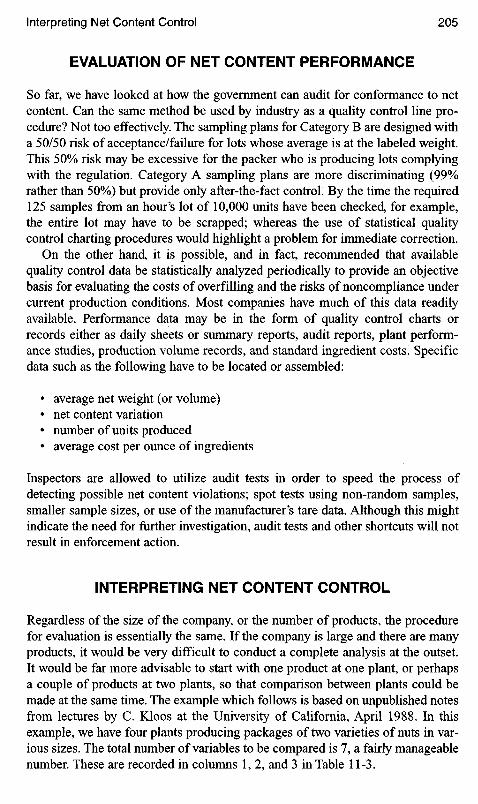
EVALUATION OF NET CONTENT PERFORMANCE
So far, we have looked at how the government can audit for conformance to netcontent. Can the same method be used by industry as a quality control line pro-cedure? Not too effectively. The sampling plans for Category B are designed witha 50/50 risk of acceptance/failure for lots whose average is at the labeled weight.This 50% risk may be excessive for the packer who is producing lots complyingwith the regulation. Category A sampling plans are more discriminating (99%rather than 50%) but provide only after-the-fact control. By the time the required125 samples from an hour's lot of 10,000 units have been checked, for example,the entire lot may have to be scrapped; whereas the use of statistical qualitycontrol charting procedures would highlight a problem for immediate correction.
On the other hand, it is possible, and in fact, recommended that availablequality control data be statistically analyzed periodically to provide an objectivebasis for evaluating the costs of overfilling and the risks of noncompliance undercurrent production conditions. Most companies have much of this data readilyavailable. Performance data may be in the form of quality control charts orrecords either as daily sheets or summary reports, audit reports, plant perform-ance studies, production volume records, and standard ingredient costs. Specificdata such as the following have to be located or assembled:
• average net weight (or volume)• net content variation• number of units produced• average cost per ounce of ingredients
Inspectors are allowed to utilize audit tests in order to speed the process ofdetecting possible net content violations; spot tests using non-random samples,smaller sample sizes, or use of the manufacturer's tare data. Although this mightindicate the need for further investigation, audit tests and other shortcuts will notresult in enforcement action.
INTERPRETING NET CONTENT CONTROL
Regardless of the size of the company, or the number of products, the procedurefor evaluation is essentially the same. If the company is large and there are manyproducts, it would be very difficult to conduct a complete analysis at the outset.It would be far more advisable to start with one product at one plant, or perhapsa couple of products at two plants, so that comparison between plants could bemade at the same time. The example which follows is based on unpublished notesfrom lectures by C. Kloos at the University of California, April 1988. In thisexample, we have four plants producing packages of two varieties of nuts in var-ious sizes. The total number of variables to be compared is 7, a fairly manageablenumber. These are recorded in columns 1, 2, and 3 in Table 11-3.

Table 1 1 -3. Net Weight Evaluation
CoMOCoI 9CoI 8CoI 7CoI 6CoI 5CoUCoI 3CoI 2CoM
Cost ($M)(CoI 4 X CoI 5 x CoI 8)
Sigmas (Z)overfilled
(CoI 8/CoI 7)Overfill
(CoI 6 - CoI 2)Sigma(RId2)
Avg. Wt.(OZ)
Cost($/oz)
Unitsproduced(millions)
Plantstate
Labelweight
(OZ)Product
630.21812.0529.2
2971.4
780.02019.22120.0810.0
5729.2
8700.6
0.170.570.78
0.37
0.120.551.390.75
0.38
0.38
0.050.200.31
0.030.160.500.90
0.300.350.40
0.250.290.361.20
16.0532.2064.31
16.0332.1664.50
128.90
0.030.030.03
0.040.040.040.04
420.1302.056.9
779.0
650.0315.5106.022.5
1094.0
1873.0
CAGANY
CAGANYCA
163264
163264
128
Walnut
Subtotal
Pecan
Subtotal
Total

We shall start by listing the total number of units produced over the past sea-son (or other period) in Column 4. These figures should be readily available fromproduction records if they are not accumulated on quality control records. It maybe more difficult to obtain the cost figures to be entered in Column 5. If the totalcosts, or labor costs, or overhead costs are difficult to obtain from the productionor accounting departments, use the more readily obtainable cost of raw ingredi-ents (and label the column accordingly). If the results of this analysis should showthat a saving of 0.5 ounces per can is possible, and if the raw ingredients cost$0.01 per can, then the conclusion would be that a $0.005 saving per can is attain-able. If labor, packaging materials, overhead, advertising, and other costs havealso been included, there might be considerable discussion as to whether thesavings also apply to these factors. Certainly, few would argue the fact that asavings of raw materials as a result of net weight savings is a real benefit. If thecosts of manufacturing can be used, combine them with raw materials and enterthis figure in Column 5.
Next, prepare Column 6 by extracting the net weights for the season (or periodof the study) from quality control records. If running averages are maintained, thisshould be easy; if not, select data from production records for an arbitrary inter-val, such as every 10th day, and calculate the average. As a guide, take about 30days worth of data. It may include "good" days and "bad" days, but they shouldnot be culled out of the data because, almost by definition, the average net weightis made up of good, bad, and indifferent days. Column 7 data (standard devia-tions) may be most readily obtained from the Range Charts (R bar/</2). Althoughsmall differences in sigma may not have any appreciable effect on the outcome ofthis analysis, average sigmas should be used if they have been revised for chartuse during the period of this study. By including minor quality control modifica-tions, this might eliminate distracting arguments during presentation of the studyat its conclusion.
Calculating the overfill for Column 8 is a simple subtraction of Column 2from Column 6. As an example, using the data for 32-ounce pecans packed inNew York, the average weight is 32.16, which is 0.16 ounces over label claim.
Column 9 is the calculated standard deviation from the mean being overfilled,or Z. (You should recall that the value for Z at the average of the distribution = 0.)This statistic is calculated by dividing the amount of overfill (Column 8) by thenet-weight standard deviation (Column 7). It will be used later in determining therisks of being out of compliance. As an example, take the 16-ounce containers ofwalnuts produced in California. The formula for Z is:
Z= (Xbar-fji)/o- = (16.05 - 16)70.30 = 0.17
This means that 16-ounce walnuts in the California plant were overfilled by0.17 standard deviations. What we have accomplished here is the conversion ofoverfill in ounces to overfill in standard deviations. This conversion will permit usto calculate the average overfill for the entire company. That, in fact, is what theaverage figure 0.38 at the bottom of Column 9 signifies: the weighted average of

overfill for all products is 0.38 standard deviations (Z =0.38). As a matter ofinterest, most companies overfill by nearly 1.0 standard deviations.
At this point, it might be wise to note that these calculations assume that thenet weights are all normally distributed. Although it may not be absolutely accu-rate to make this assumption, most distributions for filling containers are verynearly normal, with slight skewing on the low side for companies using automaticcheckweighers, and slightly on the high side for those who do not. The slightaberrations normally observed for these distributions have only a modest effecton the outcome of the calculations.
The final step in the evaluation of the performance data is the calculationof the overfill costs listed in Column 10. The calculation consists of multiplica-tion of the volume produced (Column 4) by the average amount of overfill(Column 8), times the cost-per-ounce (Column 5). For the period selected, theoverfill costs for walnuts was $2971.40; for pecans, $5729.20—with a total over-fill cost of $8700.60.
Having established the costs related to overfilling, we now proceed to theanalysis of risk associated with the weight control. The first step is to calculatethe percent of individual containers whose net weights are below the stated labelweight and enter in Column 11. This figure may be found by defining Z as thenumber of sigmas overfilled (see Column 9) and determining the area under thenormal curve below (-Z). As an example, the 16-ounce walnut containers pro-duced in California have a Z value of 0.17. By using a table for the areas underthe normal curve, it is observed that 43% of the area is below (-Z); that is, 43%of the containers for that particular product are below label weight. This might bemore easily seen from Figure 11-1.
Continuing with the calculations for Column 11, the weighted average percentbelow label weight for all of the items listed amounts to 36%. (Note that theweighted average is obtained by multiplying each value in Column 11 by thecorresponding number of units produced, as shown in Column 4. The total ofthese calculations is divided by the total number of units produced to obtain theweighted average.)
Figure 11-1. Percent below label weight (16 ounces of walnuts,California).
NET WEIGHT
Average Weight (X)«16.05Label Weight* 16.0Z = -Q.17
Z = O

Handbook 133 has defined unreasonable underfills with the establishment ofvalues for maximum allowable variation (MAV) for various classes of productweights. Values for the four weights in our example have been selected fromHandbook #133 and are listed in Table 11-4.
The minimum allowable weight is determined by subtracting the appropriateMAV from the label weight. For example, the 16-ounce package is between 0.94and 1.08, and has a MAV of 0.68. By subtracting 0.68 from 16, the minimumvalue of 15.32 results. This is entered in Column 12 of Table 11-5.
Column 13 lists the percent of individual containers which is below the mini-mum allowable net weight. The calculations are similar to those used to determineColumn 11, in which Z determines the area under the normal curve.
Minimum allowable net weight (Col 12) — Average net weight (Col 6)
a (Col 7)
As an example, the first entry in Column 13 is calculated for 16-ounce wal-nuts produced at the California plant. The individual containers could be as lowas 15.32 ounces before being declared below minimum. The percentage of suchcontainers may be found by first solving for Z in the equation above.
Z=^_^___2A3The area under the normal curve is found in the Z tables and is shown to be
0.7%. By continuing these calculations for all of the products, and taking theirweighted averages, it is shown that the company has produced, on average, 0.23%of its containers below the allowable minimum.
The next calculations will determine the probability of failing to meet the com-pliance criteria under Plan A and Plan B of Handbook 133. Under Plan A, of the30 samples selected, no more than one container may fall below the MAV, and thesample average must be no less than two standard deviations of the mean belowthe label weight. Under Plan B, of the 10 samples selected, no samples may bebelow the allowable minimum, and the sample average must be equal to or greaterthan the label declaration. A sample calculation for Plan A and for Plan B follows.
A defect is defined as a container whose net weight is below the allowableminimum. The probability of finding two or more defects in a sample of 30 is
Table 11 -4. MAV for Two Varieties of nuts
Labeled weight(pounds)
0.94-1 .081.88-2.143.90-4.707.90-9.40
MAV(decimal ounces)
0.681.122.003.00

Table 1 1 -5. Risk Analysis
CoI 18CoM 7CoI 16CoI 15CoM4CoMSCoM2CoM 1CoI 3CoI 2CoM
PlanBn=10
Plan An = 30
Plan ALimit
PlanBPr(OO)
Plan APr(OI)
(%)
BelowMAV(%)
Minimum(%)
% belowlabel(OZ)
Plantstate
(Avg %)
Labelweight
(oz)Product
29.93.50.7
17.5
35.24.10.00.9
22.1
20.2
0.20.0OO
0.1
0.40.00.0OO
0.2
0.2
15.8931.8763.85
15.9131.8963.87
127.56
6.80.080.0
3.7
2.00.00.00.6
1.2
2.2
1.90.00.0
1.0
0.20.00.00.01
0.1
0.5
0.70.0080.0
0.38
0.20.00.00.12
0.12
0.23
15.3230.8862.00
15.3230.8862.00
125.00
432822
36
45298
23
36
36
CAGANY
CAGANYCA
163264
163264
128
Walnut
Subtotal
Pecan
Subtotal
Total

expressed as Pr(O 1, n = 30) and will be entered in Column 14. Similarly, theprobability of finding one or more defects in a sample of 10 is expressed asPr(O O, n = 10) and will be entered in Column 15.
These two calculations represent the risk of being out of compliance on thebasis of individual containers in the test sample. They are based on the binomialprobability distribution where p (the percent defective) is that which is shown inColumn 13 for each product. As an example, refer to the first item in Column 13,where/? = 0.7%, or 0.007. These values are then inserted into the binomial formula:
Pr(C > 1, n = 30) - 1 - [Pr(C = O) + Pr(C = I)]
= 1 - [(0.993)30 + 30(0.007)] (0.993)29]
= 1-0.981
= 0.019 or 1.9%. This is the first entry inColumn 14 for 16-ounce walnuts producedin California.
Pr(OO, n = 10) = 1 - Pr(C= O)
= 1 - (0.993)10
= 1 - 0.932
= 0.068 or 6.8%. This is the first entry inColumn 15 for 16-ounce walnuts producedin California.
Continuing for each of the seven products, we find that the company hasa 0.5% chance of finding two or more defects in a sample of 30 (Plan A), anda 2.2% chance of finding one or more defects in a sample of 10 (Plan B).
Now that the risks of exceeding the maximum allowable variation have beendetermined, the next step is to find the risks associated with failing to reach anacceptable average weight. Under Plan A, the sample average can be no lower thantwo standard deviations of the mean Sj below the label weight. To determine theallowable limit under Plan A, first determine the value of Sj. This is found fromthe equation:
*- Vn
where S is sigma for the product (see Column 7), and n is the sample size. For16-ounce walnuts from California, we find
Sx = 0.30/V30 = 0.055
The allowable limit (Column 16) is found by subtracting 2Sx fr°m tne ^el
weight. For 16-ounce walnuts produced in California:
Allowable limit = 16.0 - 2(0.055) = 15.89
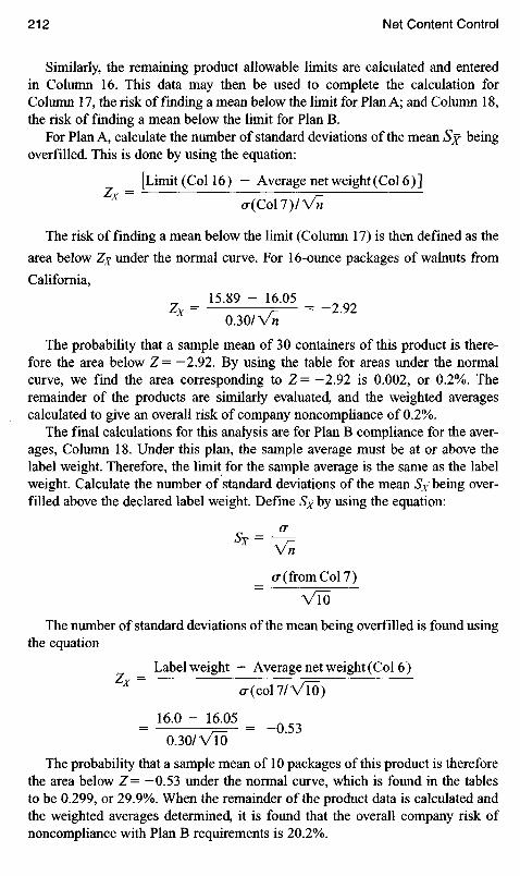
Similarly, the remaining product allowable limits are calculated and enteredin Column 16. This data may then be used to complete the calculation forColumn 17, the risk of finding a mean below the limit for Plan A; and Column 18,the risk of finding a mean below the limit for Plan B.
For Plan A, calculate the number of standard deviations of the mean SX beingoverfilled. This is done by using the equation:
[Limit (Col 16) - Average net weight (Col 6)]X Cr(CoI 1)1 Vn
The risk of finding a mean below the limit (Column 17) is then defined as the
area below Z% under the normal curve. For 16-ounce packages of walnuts from
California,= 15.89 - 16.05 =
0.30/V^
The probability that a sample mean of 30 containers of this product is there-fore the area below Z= —2.92. By using the table for areas under the normalcurve, we find the area corresponding to Z= —2.92 is 0.002, or 0.2%. Theremainder of the products are similarly evaluated, and the weighted averagescalculated to give an overall risk of company noncompliance of 0.2%.
The final calculations for this analysis are for Plan B compliance for the aver-ages, Column 18. Under this plan, the sample average must be at or above thelabel weight. Therefore, the limit for the sample average is the same as the labelweight. Calculate the number of standard deviations of the mean SX being over-filled above the declared label weight. Define SX by using the equation:si=
Vn
_ a (from Col 7)
VIoThe number of standard deviations of the mean being overfilled is found using
the equation
_ Label weight - Average net weight (Col 6)X~ a (col 7/ VlO)
_ 16.0 - 16.05 _— ,— — u. DJ
0.30/VlO
The probability that a sample mean of 10 packages of this product is thereforethe area below Z= —0.53 under the normal curve, which is found in the tablesto be 0.299, or 29.9%. When the remainder of the product data is calculated andthe weighted averages determined, it is found that the overall company risk ofnoncompliance with Plan B requirements is 20.2%.
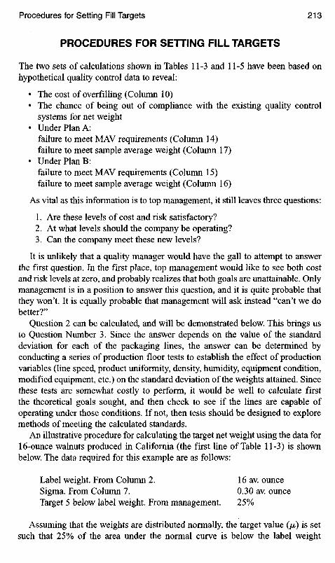
PROCEDURES FOR SETTING FILLTARGETS
The two sets of calculations shown in Tables 11-3 and 11-5 have been based onhypothetical quality control data to reveal:
• The cost of overfilling (Column 10)• The chance of being out of compliance with the existing quality control
systems for net weight• Under Plan A:
failure to meet MAV requirements (Column 14)failure to meet sample average weight (Column 17)
• Under Plan B:failure to meet MAV requirements (Column 15)failure to meet sample average weight (Column 16)
As vital as this information is to top management, it still leaves three questions:
1. Are these levels of cost and risk satisfactory?2. At what levels should the company be operating?3. Can the company meet these new levels?
It is unlikely that a quality manager would have the gall to attempt to answerthe first question. In the first place, top management would like to see both costand risk levels at zero, and probably realizes that both goals are unattainable. Onlymanagement is in a position to answer this question, and it is quite probable thatthey won't. It is equally probable that management will ask instead "can't we dobetter?"
Question 2 can be calculated, and will be demonstrated below. This brings usto Question Number 3. Since the answer depends on the value of the standarddeviation for each of the packaging lines, the answer can be determined byconducting a series of production floor tests to establish the effect of productionvariables (line speed, product uniformity, density, humidity, equipment condition,modified equipment, etc.) on the standard deviation of the weights attained. Sincethese tests are somewhat costly to perform, it would be well to calculate firstthe theoretical goals sought, and then check to see if the lines are capable ofoperating under those conditions. If not, then tests should be designed to exploremethods of meeting the calculated standards.
An illustrative procedure for calculating the target net weight using the data for16-ounce walnuts produced in California (the first line of Table 11-3) is shownbelow. The data required for this example are as follows:
Label weight. From Column 2. 16 av. ounceSigma. From Column 7. 0.30 av. ounceTarget 5 below label weight. From management. 25%
Assuming that the weights are distributed normally, the target value (//,) is setsuch that 25% of the area under the normal curve is below the label weight

(16.0 ounces). By referring to the table of areas under the normal curve, it isshown that Z (the number of standard deviations) is equal to —0.675. Solving forfju in the equation:
Label weight — /iZj —
(T
16.0 - /t
-°'675 = -53iT/x = 16.20
Therefore, a target net weight as low as 16.20 oz will result in no more than25% below the label weight as illustrated in Figure 11-2.
Selection of a 25% maximum is one way to set target weights, but it is purelyarbitrary. Another way is to select a risk of failing to comply with Handbook 133requirements. This, too, is arbitrary in that the risk is a management decision, butit is more meaningful.
As stated previously, Handbook 133 has two requirements for compliance:(1) the maximum allowable variation (MAV); and (2) the average net weight. Thefirst calculation will be to determine the target net weight needed to assure a min-imum risk of producing an unacceptable number of short-filled containers belowthe MAY Defining "minimum risk" is a management decision, but should man-agement be unwilling to provide a figure, some reasonable low risk must beassumed in order to proceed. This is not as difficult as it may appear to be. Thefigure 98% compliance is occasionally heard in relation to risk. This implies thatof the samples selected for net content evaluation by the authorities, no more than2% will be found not in compliance. From a practical standpoint, if an individualfood processor's products were sampled ten times a year, it would take 10 yearsto accumulate 100 samplings, and no more than two of those examinations mightbe out of compliance. It is not unreasonable to assume that with a 2% risk, aprocessor might have no violations for 10 times that period: 100 years!
It is possible that a company might not be selected for any sampling forseveral years. On the other hand, it is only fair to surmise that once a violationhas been observed by the authorities, that company's products will come underclose scrutiny for some time.
Figure 11-2. Selection of target weight.
Net Weight
Label veight = 16.0Z = -0.675
^16.2OZ = G

For this example, management is willing to take a 2% risk of failing thecompliance requirement for individual containers. Under Plan A, compliancerequires, at most, one defect (container below the MAV) in a sample of 30. Thisis shown as
Risk = Pr(O 1, n = 30) - 1 - [Pr(C = O) 4- Pr(C = I)]
0.02 =!-[(! -p)3Q + 30(1 -p)29 • (P)]
Solving for p (percent defective), it is found that/? = 0.007 or 7%. To solve forfji such that only 0.7% fall below the MAV (15.32 ounces), the appropriate Z valuemust first be found, using the table for areas under the normal curve. Havingfound Z= -2.455, solve for JJL using the equation
_ MAV - JULa
-2.455 = (15.32 - /i)/0.30
JLI - 16.06
This means that if the target is set at 16.06, there is a 2% risk of non-compliance for individual underfills under Plan A of Handbook 133.
Similar calculations are performed for Plan B.
Risk = Pr(OO, n=lO)=l -P(C=O)
0.02 = 1 - (1 -p)10
It might be more suitable to use logarithms to solve this equation:
(I-/?)10-0.98
101og(l-/?) = log(0.98)
log (l-p) = 0.00202
solving for antilogarithms,
(l-p) =0.9980p = 0.002, or 0.2%
The appropriate Z value for 0.2% below the MAV is —2.88. Now the calculationfor jit is completed by using the equation
-2.88 = (15.32 -/x)/0.30
jit= 16.18 ounces.
This is the target to assure 2% compliance risk for underfills under the Plan Bof Handbook 133.
Now that the calculations for MAV compliance have been calculated, thenext step is to calculate compliance for average weight. The averages are normally

distributed, with standard deviations defined as:
s,- V=Vn
The target /z, is set so that the area under the normal curve below the minimumfor the average is equal to the desired level of risk. As above, a 2% risk will beused. Under Plan A,n = 30, and the minimum sample average must be less than2 standard deviations:
Minimum = Label weight — 2Sj
- .6.0 - 2fea1LV30J
= 16.0 - 0.11
- 15.89
The appropriate Z value ( Z j ) for a 2% risk is —2.054. Therefore, the targetnet weight (/i) can be found by solving the equation
15.89 - /x-2.054 = ~=r
0.30/V30
Hence, fju = 16.00 ounces (see Figure 11-3).Under Plan B of Handbook 133, the sample size is usually 10, and therefore,
SX = 0-/VToNote that there are no allowances for the sample mean to be below the label
weight under Plan B. The desired target weight for a 2% risk can be found bysolving the equation:
16.00 - //,- 2.054 = —-
0.30/V30
Hence, ^ = 16.11 ounces (see Figure 11-4).
Figure 11-3. Compliance under Plan A.
MEAN NET WEIGHT
minimum = 15.89,
Z- = -2.054
JJl « 16.0
Z x = °

At this point, it might be wise to tabulate the results of all of the above targetweight calculations. A comparison of the two compliance programs is shown inTable 11-6. From this table, management should be in a position to select one pro-gram. The final decision may be based on an analysis of the cost/risk trade-off.To derive the relationship between the costs of overfilling and the risks of non-compliance, a company should determine the overall costs for one sigma overfill.This is useful since the overfill policy is usually expressed in terms of a certainnumber of sigmas overfill, and provides for the evaluation of alternative overfillpolicies without considering each product separately. Again, we shall use the16-ounce package of walnuts processed in the California plant. The data on whichthe calculation are based are as follows:
Label weight 16.0 ouncesAverage net weight 16.05 ouncesSigma (a) 0.30 ouncesVolume 420,100,000 units producedCost $0.03 per ounce
The cost of one sigma is found by determining the total cost of overfills, anddividing that number by the level of sigma overfill:
420,100,000 units X 0.05 ounces X $0.03 per ounce = $630,150Amount overfilled/sigma = 0.05/0.30 = 0.17
The cost of overfilling = $630,150/0.17 = $3.71 million
Criteria
25% below the label weight2% Risk of noncompliance
(a) Individual underfills(b) Sample average
Plan A
16.20 oz
16.06 oz16.00 oz
Plan B
16.20 oz
16.18 oz16.11 oz
Figure 11-4. Compliance under Plan B.
Table 11 -6. Target Net Weights for 16-OunceWalnuts, California (to comply withHandbook 133)
MEANNETWElGHT
p. * 16.1 1
Z x = °
minimum » 16.0
Z- = -2.054

Similarly, calculations for the costs for overfilling all products will provide arational means of selecting a cost/risk policy.
All of the above calculations are based on a system for complying with therequirements of Handbook 133, and selecting a risk and a cost level for eachproduct. There are other techniques which are used successfully, but to obtain theassurance that the company is in compliance, it would be advisable to run peri-odically through these calculations. Some managements may believe that merecompliance with the law is not sufficient for their product lines, and it is perfectlyconceivable that filling techniques can be improved to the point that weights arewell within the compliance limits. In general, this may be accomplished by pro-gressively reducing the sigma value for each production line through experimen-tation, training, maintenance, more uniform product, and improved equipment.Simply comparing the control limits of Jf-bar and R charts as these improvementsare introduced will point to the direction for tighter weight control. It has beendemonstrated that this technique can cut the value of sigma to the point where thetarget value of a 16-ounce container can be a scant 0.016 ounces above targetweight with no loss in productivity. The reduction of associated costs related toproduct giveaway on a high speed line are often spectacular.

12 Design ofExperiments
INTRODUCTION
Design of experiments consists of a series of techniques used to explore variousoperating conditions of a process with the goal of finding lower costs of rawmaterials, process, and product; improved product performance; less variabilityin the product; or higher production capacity to meet increasing demand. In largecompanies with specialized departments, experimental design is the province ofengineers, food scientists, or the research and development department. Qualitycontrol personnel may become involved with the performance, and possibly someof the evaluation of industrial experimentation. Consequently, an understandingof the techniques of this discipline is valuable. In smaller companies where thetask of industrial experimentation often falls to the quality control manager, aknowledge of statistical design of experiments is imperative.
It might be well to consider again the meaning of "quality." Amongst others, theclothing industry commonly uses the word to signify superior appearance orperformance. For our purposes, throughout the book, we have referred to "quality"as "a level" not necessarily a superior level or the highest level. There are manyclasses of products which need not be of high quality to perform their function;in fact high quality may be a deterrent to the marketability. Disposable toolssupplied for assembly of light-duty toys or furniture may be made of stampedsteel sheet, rather than heavy-duty, forged, chrome steel alloy. Pie-grade fruit tobe further processed into pies, jellies, or fillings need not consist of unbroken uni-form pieces. Salt used to melt sidewalk ice would gain nothing but cost if it weremanufactured to the same purity and quality level as food-grade salt. Plastic filmpackaging certainly does not exhibit the superior protective quality of hermeti-cally sealed metal containers, but many foods with short shelf life, and many withdesirable appearance which can be advantageously displayed in clear plastic neednot, and perhaps should not, be sealed in more expensive containers. Does statis-tical design of experiments have any place in industries such as these? Of courseit does. It may be possible to improve the quality level at no additional cost, thus

providing a marketing advantage even to throwaway products. It may also bepossible to design experiments which lead the way to maintaining the quality levelat higher rates of production, with less expensive or alternative raw materials, orwith less labor.
At the other end of the quality scale, a series of experiments might be designedto eliminate defects in costly food products, such as discoloration in blanchedalmonds used for stuffing prunes. Or new process methods may be explored toimprove the color retention of freeze-dried vegetable products. Or modificationof cooking methods and packaging might improve the sensory characteristics andextend the life of shelf-stable meals. The list is endless, and the opportunities toincrease profits while improving quality level are unlimited.
Occasionally the need for an experimental effort is thrust upon a processor.A frequent driving force to industrial experimentation is the threat of a changingmarket: consumers' tastes change, a competitor modifies his product, or introducesa new one. Occasionally a raw material source dries up or becomes more costlydue to weather, an increased demand from other markets, or other conditions.Disparaging press reviews of suspected environmental damage caused by a productor its packaging may force a company into a crash program of experimentation.
The main goal of a statistically designed experiment is to obtain unambiguousanswers to specific questions. Modifying a production facility or running a non-standard experimental process is expensive. There is lost production, wastedwages and overhead, and the likelihood of creating unusable scrap material. So itis of great importance that the experiment be planned sufficiently to providespecific answers, and avoid the necessity of repeating the procedure to correctmistakes made. Consider a test casually run with a modified formula, after whichthe line foreman discovers that it was produced on the wrong machine at adifferent temperature. Even if the results of the test showed an improved product,the foreman is left with doubts about the reasons for the success: was it theformula? the machine? the temperature? There is no room for careless planningor execution in a statistically designed experiment.
There is another reason for careful planning: it is rarely possible to introducea single variable in an experiment. For example, supposing a test is suggestedwhich will result in lower moisture product from a dryer by the increase of dryerair flow. It would not be surprising to find that an increase in air flow causedshorter product retention time in the dryer, and to compensate for the resultingdecrease in BTU transfer to the product, the temperature would also have to beraised. It is also rarely possible to introduce variables in a process which willdeliver a single change in the final product. In the above example, it is likely thatnot only will the moisture be affected, but the product color will probably be darkerfrom the added temperature, and the product density might well be altered appre-ciably. These new conditions may or may not be undesirable. The point to be madehere is that careful planning prior to running the experiment should eliminate sur-prises in the outcome, and should reduce the necessity of conducting additionalexperiments because of unanswered questions. The results of an experiment toshow the efficiency obtained from using large pineapples as a raw material would

indicate that a major saving in the labor force could result from eliminating manyof the trimmers and replacing them with a large-fruit mechanical trimmer. Butthis ignores the real world fact that all pineapples are not large, and that trimmerswill still be required for the normal-crop-size raw materials received during thecanning season.
The two goals of statistical design of experiments (unambiguous answers andlow-cost testing) are reached through the elimination of extraneous variables, andthe ability to handle many factors simultaneously. Extraneous variables commonlyencountered are the day-to-day differences found in any production facility: dif-ferent employees, varying motivation of the workers, environmental changes (tem-perature, humidity, light, ventilation, vibration, odor), day of the week, proximityto holidays or payday, and even local news events. For the most part, these vari-ables are related to people. There are also variables due to machines which appearto be identical but which have unique operating characteristics. When the outputof two filling machines is compared, rarely are they found to produce identicalweight dispersions. The causes may be the result of machine speed differences,wear, product flow, or machine location. Raw materials used in the process mayvary from supplier to supplier, and from hour to hour. In some industries this vari-able may be controllable: a hopper car of plastic pellets used for molding may notvary in composition from top to bottom; but a truckload of tomatoes may havedrastic quality differences due to causes as simple as location in the pile: crushedon the bottom, sunburned on the top, cold in the front. Then there are field-to-field chemical variations and maturity differences. Finally there are frequentlyuncontrolled differences between the technicians conducting the tests and theevaluators who interpret the results.
Often there are conditions under which it is not possible either to eliminatethese variables or to hold them constant. There are also circumstances under whichit would be undesirable to attempt to hold them constant. This might be the casewhere a test is under consideration to establish the ruggedness of a process whenexternal and uncontrollable variables are commonly present. Such a test might bedesigned to determine which raw ingredients may be used that are resistant touncontrollable process fluctuations, and can be depended upon to result in a uni-form quality product. It is thus important to avoid confusing essential externalvariables with experimental variables. Usually uncontrolled variables may behandled by randomly selecting them for inclusion in the test design.
There are three objectives in designing experiments. (1) All of the designfactors and all of the response variables associated with the problem beinginvestigated should be included. (2) The design factors should be appropriatelybalanced so that no factors are either overemphasized or overlooked. (3) Thereproducibility of results should be both precise and accurate. Precision refers tothe variability or uniformity of results, and is generally characterized by the stan-dard deviation, cr. Accuracy is a measure of the difference between the measuredand the theoretical results, and is expressed as (X — //,). As an example, a fillerscale might produce highly precise weights—all containers within 0.001 ounce—but the accuracy might be unacceptable at 0.75 ounce overweight.

The number of variables in a design depends on the complexity of the investi-gation, the production time available, and the cooperation of production and othermanagerial personnel. Tests designed to explore a single variable are usually theeasiest to sell to management, since they are readily understood and appear to bethe least costly to undertake. Some of the limitations have already been discussed.Experiments may be conducted off-line. There is no universal definition ofoff-line, but it generally refers to experiments conducted in the pilot plant, in thelaboratory, on commercial equipment at an equipment manufacturer's facility, oron the plant equipment when the plant is not in normal production. It is intendedto eliminate interference with production schedules, but may not necessarily bemost cost-effective.
In addition to conducting experiments with only a single variable, testing withslight changes in just a few small operating conditions at a time is frequently a suc-cessful way to design experiments. Small changes probably will not affectproduction output quantity or quality appreciably, but will show the direction forfurther improvement. Procedures of this type have been formalized as EVOP, orevolutionary operations. And a third general experimental technique examines sev-eral different operating conditions, usually over a relatively short period of time.
ELIMINATION OF EXTRANEOUS VARIABLES
ExampleWhich of four recipes makes the best cherry pie (A, B, C, or D)? In order to evaluate theproducts, the sensory testing panel requires four pies of each recipe. The laboratory isunable to bake more than four pies per day.
The most obvious solution would be to bake one pie of each type (A, B, C, and D) onone day, and submit them to the testing panel each day for four days. The problem with thissetup is that it does not take into account the day-to-day variations which may occuramongst the judges, or the changes in the laboratory personnel making up the pies. Theseare extraneous variables. The conclusions from such a test might improperly discloseapparent differences between pies which are truly differences between days.
A method which minimizes these day-to-day differences has been devised by statisti-cians and is known as a randomized block design. Under this plan, different recipes aremade up each day, but not necessarily one of each type. Over the four-day period, however,note in the plan below that each pie has been baked four times.
Day
1 2 3 4
B A C C
D C A D
A B D A
C D B B

In a randomized block design, all treatments are assigned to a block.A block is defined as a homogeneous set of conditions for comparison of thetreatments. In the above example, Days are Blocks. Again, the main purpose ofthis plan is to avoid confounding of extraneous variables with primary variables.A secondary purpose is to improve the precision by removal of effect fromexperimental error.
Another example of a randomized block design is one in which four breadformulas are compared for loaf volume when baked in a microwave oven. Theprimary variable here is the bread formula; the extraneous variable is the type ofoven used. Both the formula data and the oven data are referred to as designvariables, or design factors (variables over which the designer has control); theloaf volumes are referred to as the response variables (outcome variables).
The first step in designing this test is to develop a protocept. This is alaboratory benchtop formulation which satisfies the general requirements for theproduct to be tested. Some of the considerations might be size, weight, texture,flavor or color. Having established the attributes of the product, the protocept isthen ready to be subjected to a series of tests. It is suggested that the first tests bedesigned as simply as possible.
Note the outcomes in the table below:
Ovens
Formula GE TA SA AM
1 156 143 160 1372 150 151 157 1293 112 137 126 1094 162 151 175 149
It appears that the smallest-volume loaves are produced from Formula #3.Regardless of which oven is used, this formula produces the lowest numbers forvolume. Formula #4 produces higher volumes than any other formula for a givenoven; but also note that the 151 volume in the TA oven is smaller then the156 volume in the GE oven. This is extraneous information. The goal was to com-pare formulas, not microwave ovens. This is a one-factor design: bread formula.
An alternative plan for the four-recipe pie-baking problem above is called theLatin Square. It is designed to control for two blocking factors: Day andSequence. You will note in the Latin Square below that each pie is baked onlyonce on each day, and that the first pie baked is different each day. This eliminatesthe possibility of drawing incorrect conclusions in the event that the first piebaked is always different than subsequent pies due to lack of oven prewarming.The two extraneous variables here are (1) the day the pies were baked, and (2) thesequence of baking.

Day
Sequence 1 2 3 4
1 A D C B2 B A D C3 C B A D4 D C B A
When a large number of variables must be compared at the same time, a mod-ification of the randomized block design may be used. Assume that we wish tocompare seven pie recipes. The sensory panel judges can evaluate no more thanthree pies before losing their ability to detect flavor differences. The design whichsatisfies these requirements is called an Incomplete Block Design. The sevenrecipes for pies are shown as A through G below. Note that each judge evaluatesonly three pies, and that each pie is sampled by three different judges. The designis carefully balanced so that each group appears the same number of times, andeach formula appears the same number of times. Note also that the pair AE occursonly once, as does the pair AC, EC, etc.; that is, each pair of recipes appears onlyonce. In this manner, each pie recipe can be compared independently of judge-to-judge variation. Prepared tables of incomplete block designs are available in theliterature.
Judge
1 2 3 4 5 6 7
A G A C B C DE F B G E D GC A D B F F E
The following are several commonly used examples of incomplete blockdesigns (Table 12-1).
Statisticians have developed many types of block designs to handle experi-ments other than the simple ones shown above. A list of the most commonly usedblock designs follows:
• Randomized block• Balanced incomplete block• Latin squares• Graeco-Latin squares (for 3-block variables)• Hyper Latin squares (for more than 3 variables)• Incomplete Latin squares.

Table 12-1. Incomplete Block Designs
Block Treatments Block Treatments Block Treatments
(1) 4 Treatments, 2 per block123456
a bc da cb da db c
(2) 5 Treatments, 2 per block12345
a bc db ea cd e
6789
10
a db cc ea eb d
(3) 5 Treatments, 3 per block12345
a b ca b ea d eb e dc d e
6789
10
a b da c da c eb e eb d e
(4) 6 Treatments, 2 per block12345
a bc de fa cb e
6789
10
d fa db fc ea e
1112131415
b dc fa fb cd e
(5) 6 Treatments, 3 per block12345
a b ea b fa c da c fa d e
6789
10
b e db e eb d fc e fd e f
(6) 7 Treatments, 3 per block1234567
a b db e ec d fd e ga e fb f ga c g

HANDLING MANY FACTORS SIMULTANEOUSLY
Looking at the cherry pie formulation from another viewpoint, suppose we areinterested in evaluating the effect of three factors:
• Butter (B) versus margarine (M)• Cherry supplier A or B• Amount of sugar—high or low.
The number of pies which can be baked is restricted to four. A typical non-statistical method which might be used would be to change one variable at a time.The first pie would contain butter, cherries from supplier A, and low sugar. Next,a pie would be baked using margarine, but otherwise the same as the first one.The third pie would be the same as the first, but with cherries from supplier B;and the fourth pie would be the same as the first, but with a high level of sugar.This arrangement is shown below:
Nonstatistical plan
Shortening Cherries Sugar
B A LOM A LOB B LOB A HI
This plan adequately compares some of the pie variables with the first pie, butdoes not cover all of the interactions. For example, there is no formula tocompare the first pie with one made with margarine and high sugar; nor is therea pie with margarine and cherries from supplier B. To include all of the combi-nations would require many more pies than could be baked at one time, but withthe four combinations above, it is obvious that the three variables are not treateduniformly Only one test uses margarine, and three use butter; only one test hashigh sugar, and three have low.
By using a statistical plan, some of these deficiencies may be overcome. In thestatistically designed plan below, each variable is examined the same number oftimes: two butters and two margarines; two high sugars and two low sugars; twosupplier A and two supplier B. Note also that each variable is tested one timeagainst each of the other variables: for example, butter (B) is tested with supplierA and supplier B, and with high and low sugar. By examining the plan below, itis found that all of the variables are similarly compared once with each other.
One example of the advantage of the statistical plan over the nonstatistical planis the fact that the statistical plan will compare the effect of butter over margarinefor each supplier, and at each level of sugar. The nonstatistical plan does not

Statistical plan
Shortening Cherries Sugar
B A LOB B HIM A HIM B LO
compare the effect of butter over margarine either for supplier B, or for highsugar. Another advantage of the statistical plan is that all of the formulas areused in estimating the effects. The shortening effect is the difference between theaverage of the first two formulas and the average of the last two formulas. Bybeing able to use averages, the standard error is reduced by a factor of \R(2). Thissmall standard error enables the statistical plan to detect small differences.
The types of multifactor experimental plans which handle many factors simul-taneously to be discussed are:
• Full factorial designs• Fractional factorial designs• Response surface design• Mixture designs.
FULL FACTORIAL DESIGNS
A full factorial design will include all possible combinations of all of the condi-tions. In the case of the cherry pie tests above, if there had been no restrictions onthe number of pies baked at one time, a full factorial design might have been used,and would appear as shown below:
Shortening Cherries Sugar
B A HIB A LOB B HIB B LOM A HIM A LOM B HIM B LO
The simplest factorial design is called a 2 by 2 design. It considers theresponses of a test in which two factors (variables) are examined at two levels

Table 12-2. 2x2 Factorial Experimental Design Conditions
Condition number
1234
Concentration (%)
13.514.513.514.5
Temperature (0C)
124124128128
Concentration
Figure 12-2. Data from a 2 x 2 experiment.
I— <D
£CL
CD
»-aJ-i-i3»-<D
Figure 12-1. A 2 x 2 design.
Concentration
I— o>
£Q
_<
D>
-cCi-:3
i_a>
(values). In the following example, two variables (temperature and concentration)will be studied at two levels (low and high). The response to be evaluated shall bethe yield of the process. A diagram representing the experiment is shown inFigure 12-1.
A total of four conditions will include all of the possibilities for conductingthis test design. (See Table 12-2.)

Table 12-3. 2x2 Factorial Experimental Design Data
Condition number Concentration (%) Temperature (0C) Yield
1 13.5 124 60.22 14.5 124 67.63 13.5 128 73.24 14.5 128 76.2
The experiment is subsequently conducted under these four sets of conditions,yielding the results shown in Figure 12-2 and Table 12-3.
Examining the effects of increasing the concentration from 13.5 to 14.5%:
Concentration effect
67.6-60.2 = 7.4 @ temperature 1240C76.2 - 73.2 = 3.0 @ temperature 1280C
71.9 - 66.7 = 5.2 Average yield
The yield increases at either temperature, but to a greater extent at124 degrees. If the process were to be operated at the higher concentration, wemight expect that the lower the temperature (between 124 and 128), the better theyield.
Temperature effect
73.2 - 60.2 = 13.0 @ concentration 13.576.2-67.6 = 8.6 @ concentration 14.5
74.7 - 63.9 = 10.8 Average yield
Similarly, increasing the temperature while holding the concentration at13.5%, the yield increases by 13.0%. At the high concentration, increasing thetemperature increases the yield by 8.6% From this simple design, a surprisinglylarge amount of useful information emerges.
The interaction effect can be quantified as well. The difference between theconcentration effect from high temperature to low temperature is 7.4 - 3.0 = 4.4.The difference between the temperature effect from high concentration to lowconcentration is 13.0 - 8.6 = 4.4. It might be expected that one would measurethe interaction as 4.4, but the definition used by statisticians is based on 1/2 ofthis difference, and would be expressed as 2.2 ± 2.2. To explain the interaction

effect, consider the following:
If there were no interaction effect, the main effects of both variables would bethe same at both levels of the other variable. That is:
Concentration effect = 5.2 @ temperature = 124 0C and 128 0CTemperature effect = 10.8 @ concentration = 13.5% and 14.5%
If we now consider the actual effects at the high level of the other factor:
Concentration effect = 3.0 @ temperature = 128 0CTemperature effect = 8.6 @ concentration = 14.5%
And the interaction results in the following:
Interaction effect = 3.0 - 5.2 = -2.2 and 8.6 - 10.8 = -2.2
The graph in Figure 12-3 answers the question "does it matter what thetemperature level is when the concentration changes are examined?" It is obviousthat there is a large difference in yield when moving from 13.5% to 14.5% con-centration on the 124-degree temperature graph; and there is a smaller differencein yield when moving from 13.5% to 14.5% concentration on the 128-degreetemperature graph. By changing the graphed axes to yield and temperature, theeffect is again observed: there is a larger effect at 124 degrees than at 128 degrees(Figure 12-4).
As a matter of interest, the yield values 60.2, 67.6, 73.2 and 76.2 in theabove example were taken from an actual test, and although only a single value
TEMPERATURE = 128
TEMPERATURE = 124
CONCENTRATION
Figure 12-3. Interaction plot of concentration by temperature.
YIE
LD
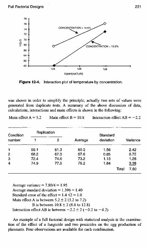
TEMPERATURE
Figure 12-4. Interaction plot of temperature by concentration.
was shown in order to simplify the principle, actually two sets of values weregenerated from duplicate tests. A summary of the above discussion of data,calculations, interactions and main effects is shown in the following:
Main effect A = 5.2 Main effect B = 10.8 Interaction effect AB = -2.2
YIE
LD
CONCENTRATION = 13.5%
CONCENTRATION = 14.5%
Conditionnumber
1234
Replication
1
59.168.272.474.9
2
61.367.074.077.5
StandardAverage
60.267.673.276.2
deviation
1.560.851.131.84
Variance
Total
2.420.721.283.38
7.80
Average variance = 7.80/4 = 1.95Average standard deviation — 1.396 ~ 1.40Standard error of the effect = 1.4 V2 = 1.0Main effect A is between 5.2 ± 2 (3.2 to 7.2)
B is between 10.8 ± 2 (8.8 to 12.8)Interaction effect AB is between -2.2 ± 2 (-0.2 to -4.2)
An example of a full factorial design with statistical analysis is the examina-tion of the effect of a fungicide and two pesticides on the egg production ofpheasants. Four observations are available for each combination.

Pheasant Egg Counts
Pesticide levels
None Level A Level B
No fungicide15 29 7 15 17 1918 30 9 18 16 21
With fungicide12 15 13 10 9 1110 9 6 8 14 13
An analysis of variance shows that there is an effect from both the fungicideand from the pesticide.
Analysis of variance
Source df M.S. F
Fungicide 1 294.00 16.04 (P<0.01)Pesticide 2 87.17 4.75 (P<0.05)FXP 2 36.50 1.99Error 18 18.33
There is an effect both from the fungicide and from the pesticide.Full factorial designs are used if there are only two or three factors to explore.
They are also useful in the event of higher order interactions. That is, some factorshave little effect on outcomes of an experiment until a threshold is reached, afterwhich the effect may be significant. It is interesting to note that the statistician maybe unaware of these interactions, and must depend on the experience of qualitycontrol or line personnel to provide information on their importance so thatthey may be incorporated into the experimental design. Another application requir-ing full factorial design is for analyzing qualitative independent variables, suchas the number of different suppliers of raw materials. If there are four suppliersavailable, all four must be included in the test plans.
FRACTIONAL FACTORIAL DESIGNS
Fractional factorial designs are used when there is a large number of possiblecombinations of variables, and are generally applied when the factors may occurat two levels. The fraction selected depends on assumed interactions, and mustcome from a statistical design. An example might be a process with six variablesoccurring at two levels. The total number of interactions is 64> and it is highlyunlikely that management would agree to shutting down a line in order to run 64separate experiments! Information for all of the two-factor interactions would

require only 32 tests. Only 16 tests would be required to investigate some of thetwo-factor interactions; and if no two-factor interaction information were required,only eight tests would be needed, hi common practice, an experimenter needs infor-mation on only a few of the interactions, and a complete series is rarely run. Fractionalfactorial plans are useful when the higher order interactions referred to above are ofno particular importance. This type of plan may be effective when only the maineffects of the variables are of interest; that is, when "screening" tests are required.
The eight-test screening plan generates sufficient information to identify whichof the variables (e.g., ingredients) have the greatest significance on the outcome ofthe problem being evaluated. This should further reduce the number of detailed testsrequired to isolate exact differences. If these eight tests had disclosed that of the sixingredients in the formula, two were of importance and four had virtually no sig-nificance, then subsequent tests need be concerned only with those two ingredients.
The following example of a fractional factorial was designed to measure theresponse (Y) of variations in eight ingredients at two levels of concentration in acat food mix (Table 12-4). Note the balanced nature of this test plan: the low lev-els of A (17), which are matched with the low levels of B (7), appear four times;the high levels of A (26), which are matched with the high levels of B (13), alsoappear four times. Likewise, there are four tests each for the high-low and thelow-high combinations of ingredients A and B. Similar two-level pairs are foundthroughout the test plan for the eight ingredients and the 16 tests.
From the analysis of variance (Table 12-5), it becomes apparent that ingredi-ents A, D, and E are the ones that truly have a large effect on the response. Thisscreening test has therefore revealed the three ingredients which will require fur-ther experimentation.
Table 12-4. Eight-ingredient Cat Food Test Levels and Responses
Ingredients Response
A B C D E F G H Y
1 7 7 5 2 O O 6 3 0.922 6 1 3 1 1 5 O 0 6 3 1.4417 7 5 2 0.5 25 12 4 1.4326 13 11 5 0.5 25 12 4 1.912 6 1 3 5 2 O 2 5 6 3 1.742 6 1 3 5 2 0 . 5 O 1 2 4 1.2817 7 11 5 O 25 6 3 1.7717 7 11 5 0.5 O 12 4 1.3226 7 5 5 O O 12 3 2.032 6 7 5 5 0 . 5 2 5 6 4 1.4617 13 11 2 O O 12 3 1.4517 13 11 2 0.5 25 6 4 1.002 6 7 1 1 2 O O 6 4 1.6526 7 11 2 0.5 25 12 3 1.171 7 1 3 5 5 O 0 6 4 1.671 7 1 3 5 5 0 . 5 2 5 1 2 3 1.29

Table 12-6 consists of several commonly used examples of Fractional Factorialdesigns.
Table 12-5. Analysis of Variance
Source df M.S. F
A 1 0.14251 9.55 P<.05B 1 0.00766 0.51C 1 0.00276 0.18D 1 0.23281 15.60 P<.01E 1 0.74391 49.86 P<.01F 1 0.00681 0.46G 1 0.00051 0.02H 1 0.00331 0.22
Error 7 0.01492
Table 12-6. Fractional Factorial Designs
a b c d e f g h a b c d e f g h Effects df
1/2 rep of a 24 factorial0 0 0 01 1 0 01 0 1 01 0 0 10 1 1 00 1 0 10 0 1 11 1 1 1
Main2-factor
Total
43
7
AB = CD, AC = BD, AD - BC
1/4 rep of a 25 factorial0 0 0 0 01 1 0 0 00 0 1 1 01 0 1 0 10 1 1 0 11 0 0 1 10 1 0 1 11 1 1 1 0
Main2-factor
Total
52
7
Main effects have 2-factor aliasesAC = BD, AD = BC
1/2 rep of a 25 factorial0 0 0 0 01 1 0 0 01 0 1 1 10 1 1 1 10 0 1 0 0
1 0 0 0 10 1 0 0 10 0 1 1 01 1 1 1 01 0 0 1 0
Main2-factorTotal
51015

Table 12-6. (continued)
a b c d e f g h
0 1 1 0 00 0 0 1 11 1 0 1 0
a b c d e f g h
0 1 0 1 00 0 1 0 11 1 1 0 1
Effects df
1/8 rep of a 26 factorial0 0 0 0 0 01 0 1 0 0 1
1 0 0 1 1 00 1 1 0 1 00 1 0 1 0 11 1 1 1 0 01 1 0 0 1 10 0 1 1 1 1
Main2-factor
Total
61
7
Main effects have 2-factor aliasesAB = CD = EF
1/4 rep of a2 factorial0 0 0 0 0 0 11 1 1 0 1 0 01 1 0 1 0 1 00 0 1 1 1 1 11 0 1 1 0 0 11 0 0 0 1 1 10 1 1 0 0 1 00 1 0 1 1 0 0
1 0 0 0 00 1 0 1 00 0 1 0 11 1 1 1 10 1 0 0 10 0 1 1 01 1 1 0 01 0 0 1 1
Main2-factorError
Total
672
15
AC = BE, AD = BF, AE = AC, AF = AD, CD = EF, CF = DE, AB - CE = DF
1/16; rep of a 27 factorial0 0 0 0 0 0 01 1 1 1 0 0 01 1 0 0 1 1 01 0 1 0 0 1 11 0 0 1 1 0 10 1 1 0 1 0 10 1 0 1 0 1 10 0 1 1 1 1 0
Main
Total
7
7
1/8 rep of a 27 factorial0 0 0 0 0 0 00 0 0 0 1 1 11 1 1 1 0 0 01 1 1 1 1 1 11 1 0 0 0 0 10 0 1 1 0 0 11 1 0 0 1 1 00 0 1 1 1 1 0
1 0 1 0 0 1 00 1 0 1 0 1 01 0 1 0 1 0 10 1 0 1 1 0 11 0 1 0 1 0 00 1 0 1 1 0 01 0 1 0 0 1 10 1 0 1 0 1 1
Main2-factorError
Total
771
15
AE = BF = CG, AF = BE = DG, AG = CE = DF, BG = DE = CF, AB = CD = EF,AC = BD = EG, AD = BC = FD

Table 12-6. (continued)
a b c d e f g h a b c d e f g h Effects d f
1/6 rep of a 28 factorial0 0 0 0 0 0 0 0 1 0 0 1 1 0 1 1 Main 81 1 1 1 0 0 0 0 1 0 0 1 0 1 0 1 2-factor 70 0 0 0 1 1 1 1 0 1 1 0 1 0 1 0 Total 1 51 1 1 1 1 1 1 1 0 1 1 0 0 1 0 11 1 0 0 1 1 0 0 1 0 1 0 1 0 0 11 1 0 0 0 0 1 1 1 0 1 0 0 1 1 00 0 1 1 1 1 0 0 0 1 0 1 1 0 0 10 0 1 1 0 0 1 1 0 1 0 1 0 1 1 0AE = BF = CH = DG, AG = BH - CF = DE, AC = BD = EH = FG, AB = CD -EF-GH.
AF - BE = CG = DH, AH = BG = CE = DF, AD = BC = EG = FH
RESPONSE SURFACE DESIGNS
After conducting fractional factorial experiments to determine which factors areof importance, the next step is to explore the interrelationships of these factors byuse of response surface designs. The goal here is to find the best combination ofthe variables.
As an example, consider the pressure, time, and temperature needed to applya plastic cover onto a container to maximize burst strength. In the chapter cover-ing regression analysis (Chapter 12), only two variables were involved: the rela-tion between Y and X. In the case of three variables, the model equation becomesmore complicated.
Variables:
XI Temperature
X2 Time
X^ Pressure
Outcome:
Y Burst strength
Model:
Yift = BQ + B\XI + B2X2 + 3 3 + l \X\ + B22X2 + #33-^3 +.#12^V^2
+ B\^X\X^ ~\~ 823X3X3 " " EE = Experimental error.
The central composite design (see Figure 12-5) is the classic design for responsesurface designs. Each side of the cube represents one of the three variables.
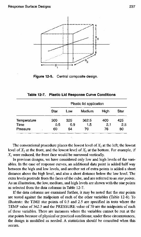
Figure 12-5. Central composite design.
Table 12-7. Plastic Lid Response Curve Conditions
Plastic lid application
Star Low Medium High Star
Temperature 300 325 362.5 400 425Time 0.5 0.9 1.5 2.1 2.5Pressure 60 64 70 76 80
The conventional procedure places the lowest level OfX1 at the left; the lowestlevel ofX2 at the front, and the lowest level of X^ at the bottom. For example, ifXI were reduced, the front face would be narrowed vertically.
In previous designs, we have considered only low and high levels of the vari-ables. In the case of response curves, an additional data point is added half waybetween the high and low levels, and another set of extra points is added a shortdistance above the high level, and also a short distance below the low level. Theextra levels protrude from the faces of the cube, and are referred to as star points.As an illustration, the low, medium, and high levels are shown with the star pointsas selected from the data columns in Table 12-7.
If the data columns are examined further, it may be noted that the star pointsare tested against the midpoints of each of the other variables (Table 12-8). Toillustrate: the TIME star points of 0.5 and 2.5 are specified in tests where theTEMP value of 362.5 and the PRESSURE value of 70 are the midpoints of eachof these variables. There are instances where the variables cannot be run at thestar points because of physical or practical conditions; under these circumstances,the design is modified as needed. A statistician should be consulted when thisoccurs.

After running the tests and obtaining the outcome information, a linear regres-sion analysis is utilized to determine the equation relating the variables. From theabove data, a stepwise linear regression analysis produced the following model:
Y= 8.925 - 0.00238*Temp - 11.059*Time + 0.0333*Temp*Time
The remaining Bs were nonsignificant. The pressure variable had no effect onthe burst strength. Using the equation, it is possible to determine the burststrength for any combination of time and temperature selected. Note that althoughonly five different levels of variables were examined in the test procedure, theresulting equation permits calculating the burst strength for any combination offactors. By constructing a graph of this equation, the values of all variables canreadily be selected (Figure 12-6).
Using the chart, select a temperature of about 300° and a time of 2 s, the burststrength will be about 6; a temperature of 350° and a time of 1.5 s will producea burst strength of 9; or 375° for 0.7 seconds will produce a 9 burst strength.(The curves are read in the same manner as contour maps.)
Whenever a series of experiments is performed to produce a response surface,it is wise to select the best combination of points and retest them to prove that thedata are reliable, and that the calculations were correct. In some instances, theresponse surface analysis will show that more than one set of conditions appear
Table 12-8. Plastic Lid Experimental Design and Outcome
Experiment conditions
X1 Temp
325325325325400400400400300425362.5362.5362.5362.5362.5
X2 Time
0.90.92.12.10.90.92.12.11.51.50.52.51.51.51.5
X3 Pressure
647664766476647670707070608070
Experiment outcome
/(duplicate tests):Burst strength
8.758.257.508.50
10.5010.0012.0013.004.00
12.758.75
11.009.259.759.25
7.59.07.09.59.75
10.013.7512.57.0
12.08.5
10.259.09.59.5

Figure 12-6. Contour plot of burst strength.Credit: Wendell Kerr, Calreco, unpublished manuscript.
to be optimum, and it is again important to verify this information in "the realworld."
Response surface plans are used where functional relationships are desired,and where the independent variables are quantitative. Variables such as "Supplier A"and "Supplier B," or machine #31 versus machine #12, cannot be consideredsuitable for this design. If there are more than five variables in the system, it isadvisable first to run a screening design to eliminate some of the variables; other-wise, the testing becomes too large to handle.
Some applications for response surface designs may appear relatively trivial,but may result in substantial reduction in costs or improvement in quality. In thepotato processing industry, peeled potatoes pass over an inspection belt whereinspectors remove grossly defective potatoes, followed by trimmers who removedefects after the potatoes have been cut into french fries. If a fixed number ofworkers is available for the process of removing defects, the question arises: howshould the workers be allocated between inspection and trimming? Of 12 work-ers, should 3 be used as inspectors and 9 as trimmers, or should it be 6 and 6? Byuse of response surface analysis, the optimum allocation may be determined. Thevariables in such a test would be the numbers of inspectors and trimmers; the out-come would be the number of defects per pound after both operations.
MIXTURE DESIGNS
Mixture design is a special response surface type since the total of the variablesmust equal 100%. In the temperature/time/pressure example above, there is no
TEMPERATURE
fUSff OFTO
C
IN

such requirement. Where the variables must equal 100% (X1 +X2+X3 = 100),the general equation
Yijk = BQ + B]X] + B2X2 + B3X3+ B1 ,X12 + B22X2
2 + B33X32 + BUX}X2
+ B^3X]X3 + B23X2X3 + hi
becomes greatly simplified to:
Y — B]X] + B2X2 + B3X3 + B]2X]X2 + B]3X]X3 + B23X2X3 + E
In the following example, three types of fish are available for use in preparingfish patties: mullet, sheepshead, and croaker (Table 12-9). The experimentaldesign is:
Variables:
X] Mullet
X2 Sheepshead
X3 Croaker
Outcome:
Y Mixture flavor
The fitted model is:
Y= 4.2X1 + 5.IX2 + 3.9X3 - 3.6X1X3 + 1.8X1X3 + 0.6X2X3
As previously, after running the tests and obtaining the responses, the data areamlyzed to arrive at a model equation relating the variables. A graph of the model
Table 12-9. Fish Flavor Experiment Design and Outcome
Experiment conditions
X1
% Mullet
100OO
5050
O33
X2
% Sheepshead
O100
O50
O5033
Experiment outcome
X3% Croaker
OO
100O
505033
YFlavor
4.25.13.93.8, 3.64.4, 4.54.5, 4.74.4,4.2,4.3

is read as follows: the flat side of the triangle opposite the labeled apex is the zerolevel of that variable (see Figure 12-7), and the apex is the 100% level for that vari-able. The center point of the triangle is a mixture containing equal amounts of eachof the three fish in the blend. Examining either the model or the chart, it becomesapparent that the better flavored blends contain higher sheepshead proportions.
One of the limitations of this type of analysis is that rarely can each ingredientbe used at levels from zero to 100%. It is not possible to go from 0% to 100%sugar in hot cocoa mix, for example. The final cocoa mix must contain cocoa,milk solids, fats, salt, and many other components.
In some instances it is possible to apply limits; in other instances the totalformula might be reduced to some of the key ingredients for purposes of experi-mentation. In such cases, the final trial run of some of the key findings becomesimperative, in order to test their validity. The need for the final test may bedemonstrated in designing tests of dry soup mix, where the salt content may bepermitted to vary from zero to 8%. In the event that the "best" mixture for souphas a salt content of 6%, it might be found by actual testing that this level is toohigh because of interfering flavor characteristics of the other ingredients. It isunlikely, of course, that such a situation would exist near the set points ofthe actual experiment, since each of these is evaluated for flavor as the "outcome."At intermediate points, however, there is always a possibility of unusual flavorcombinations which should be subsequently confirmed.
HuI let*1
M3
OfNatfaw*
K5She $hftBd
Figure 12-7. Contour plot of flavor.Credit: John A. Cornell, Experiments with Mixture Designs, Models,and the Analysis of Mixture Data (New York: John Wiley & Sons).

The graphical representations for response surfaces become increasinglycomplex as the number of variables increases, and this, among otherreasons, accounts for the limitation of five variables for this type of analysis.For example, if a fourth fish were added to the fish patty experiment, the result-ing chart would be a three-dimensional tetrahedron. This is dramatically moredifficult to interpret.
The following example represents a practical problem which illustrates acentral composite design experiment leading to a response surface analysis.The problem is to set the color specifications on a processed tomato product,using the trichromatic color system. The system currently in use measuresreflectance of the product and expresses the results on a scale of white-to-graywhich does not always represent satisfactorily the red color perceived by theeye. The trichromatic technique of measuring color provides numerical valuesfor Chroma (brightness), Hue (redness), and Value (lightness to darkness), andis thought to be more reproducible and more characteristic of visual percep-tion. In addition to these objectives, management requested that the specifica-tions be set as simply as possible, preferably by use of a single range ofnumbers, rather than the three number sets normally used with the newer sys-tem. To assist in developing realistic specifications, management has directedthat consumer testing be utilized to establish likes and dislikes of productcolor.
In the examples above, the equation terminology has been based on B and Xrelationships. There is no complete agreement on nomenclature. The researcherfor this color problem used a different group of identifiers, but note that the formof the mathematical model is identical.
CR -/(Hue, Chroma, Value)CR = AQ + AI Hue + A2 Chroma + A3 Value + An Hue X Chroma
+ A13 Hue X Value +A23 Chroma X Value +An Hue2
+ A22 Chroma2 + A33Value2
In order to develop a continuous scale of consumer response, it was considerednecessary to provide each subject with a nine-point hedonic rating scale for eval-uation, rather than the two or three points which have been used in some of theprevious samples. The rating scale consisted of the following:
• Dislike extremely• Dislike very much• Dislike moderately• Dislike slightly• Neither like or dislike• Like slightly• Like moderately• Like very much• Like extremely

The central composite design selected for this experiment requires 15 samplesto fit the model:
23 factorial points 8Star points above each face 6Center point 1
Total 15
A pictorial model (Figure 12-8) shows the location of the 15 points.The experimental design is constructed in the same manner as the plastic lid
application example above. Compare the selection of matched variables in thetwo examples (Table 12-10).
Figure 12-8. Central composite design.
Table 12-10. Tomato Product ColorExperimental Design
Point
123456789101112131415
Hue
343434344646464631494040404040
Chroma
444456564444565650504159505050
Value
20302030203020302525252517.532.525

If it were possible, each consumer would be asked to rate all fifteen samplesand the control; however, fatigue would reduce the sensitivity of the test, and asimpler arrangement is required. By using a balanced incomplete block design,each consumer evaluates 8 samples, as shown in Table 12-11. The number of con-sumers needed to balance the design is governed by the relationship: BXK =RXT, where
B = number of consumersK = number of samples evaluated by each consumerR = number of times each sample is evaluatedT= number of samples being tested
For this test,K= 8, T= 15, R was specified at 50
5 X 8 - 5 0 X 1 5
5 = 93.75We chose R - 48, which yields:
5X8 = 48X155 = 90
In order to meet the required number of consumers (5 = 93.750), it will be nec-essary to repeat the above design six times (15X6 = 90), randomizing the order
Table 12-11. Consumer Responses
Sample presentation order
Consumer No. I Il III IV V Vl VII VIII
1 11 4 2 5 10 3 14 152 4 1 3 15 13 11 6 93 9 2 14 4 7 1 10 134 15 3 1 10 8 13 7 55 7 13 10 12 11 2 3 66 6 10 12 1 4 14 8 37 12 9 13 14 15 10 11 88 1 0 1 1 9 7 6 8 5 49 5 14 7 3 1 9 12 11
10 8 15 6 2 3 7 9 1411 1 7 11 8 2 4 15 1212 2 6 15 9 5 12 1 1013 13 8 5 11 14 6 2 114 14 5 4 6 12 15 13 715 3 12 8 13 9 5 4 2
Note: T= 15 samples; k= 8 samples/consumer; B= 15 consumers.

of sample presentation. The test was completed and the average response for eachsample was calculated and tabulated. The consumer hedonic rating for eachsample is tabulated in Table 12-12.
To simplify the statistical analysis, it is necessary to eliminate one column ofvariables. The variables removed from the analysis for the present are the data forvalues. This, in effect, reduces the cube model to a square, with nine responses toconsider instead of the 15 available.
These nine responses (plus the five center-point replicates) are selected andshown in Table 12-13 as a subset. Following the columns of data, the consumerresponse mathematical model is shown with the value variables omitted.
Table 12-12. Average Consumer Responses
Sample no. Hue Chroma Value Average response
1 34 44 20 4.182 34 44 30 3.193 34 56 20 5.494 34 56 30 5.085 46 44 20 4.386 46 44 30 4.697 46 56 20 5.43etc. etc. etc. etc. etc.
Table 12-13. Simplified Model with Value Responses Omitted
Sample no. Hue Chroma Response
1 34 34 4.182 34 56 5.493 46 44 4.384 46 56 5.435 31 50 3.236 49 50 6.217 40 41 3.748 40 59 6.109 40 50 5.6210 40 50 6.1011 40 50 5.6612 40 50 5.6113 40 50 5.7614 40 50 5.9115 40 50 5.91

The simplified model is then solved using the data:
Consumer response (CR) = A0 + A1 X Hue + A2 X Chroma + A\\ X Hue2
+ A12X Hue X Chroma + A22 X Chroma2
Using a regression analysis computer program, the following equation isobtained:
Consumer response (CR) = -52.23 + 1.16 X Hue +1.2OX Chroma-0.01336 X Hue2-0.01090 X Chroma2
or
0.01336 (Hue - 43.4)2 + 0.0109 (Chroma - 55)2 - (5.9 - CR)
Since CR = 5 = neither like nor dislike, the right-hand term above becomesapproximately 6-5 which — 1. Therefore,
(Hue - 43.4)2 (Chroma - 55)2 _
6737 + 82^57 " *
The best reponses are Hue at 43.4 and Chroma at 55.0.
As we have seen before, one of the advantages of this type of analysis is thatthe intermediate points of consumer preference may be extrapolated without con-ducting another series of experiments. The easiest way to do this is graphically. Thegraph of the response surface is approximated in Figure 12-9. The intersection ofthe two axes has a value of 43.4 Hue and 55.0 Chroma, with a hedonic responseof 6.5 (the maximum preference rating of all of the consumers). The inner ringwould have a value of 6.0; the intermediate ring, 5.5; and the outer ring 5.0. It istherefore possible to interpret consumer preferences at any combination of values.
Figure 12-9 shows a small portion of the total response surface, and may bethought of as the upper surface, with the observer standing above it, and lookingdown. A computer printout of the entire surface is shown in Figure 12-10, andrepresents a three-dimensional picture.
Figure 12-9. Surface response-elliptical contours.
HUE
CHROMA
H=43,3C=55.0
CR = 6.5
CR=6.G
CR=5.5
CR=5.0

Figure 12-10. Complete response surface.Credit: Ransall Hamlin. The Place of Design in Process Improvement (Hunt Wesson Foods,Inc. 1987), K-116.
Returning to the initial statement of the experimental design goal, a singlerange of numbers may be selected as a color specification. An initial candidatefor such a specification might be: if a consumer rating is above 5.5, accept thesample; if the score is below 5.5, resample. If resample is above 5.5, accept—otherwise reject.
The question of what to do if the value variable were also significant shouldbe mentioned. If value were included along with hue, chroma and response, amathematical solution would require a four-dimensional model—extremely diffi-cult to depict! It would be wise to consult with a statistician, who might proposea compromise. The compromise method is to use only two of the variables andthe response, as we have done here, then extract a slice from the model whichincludes the required specification levels, and then proceed to repeat the experi-ment (in whole, or in part) with value, response, and one of the other variables.For a complete test, a second replicate test would be required with the remainingvariable. If the color problem is a critical one, the entire series of tests will be nec-essary; otherwise, a few spot values may be tested to "rough out" the location ofspecification levels for all the variables.
Elliptical contours are particularly useful since they define maximumresponses. There are many other contours which are less desirable. One of theseis the so-called saddle point response (Figure 12-11). The intersection of the axesis not the maximum response, but an intermediate value from which moving in

Figure 12-11. Saddle point contours.
a vertical or right horizontal direction shows increasing responses, and conversely,moving down or to the left shows decreasing responses.
EXPERIMENTAL DESIGN ANALYSIS BY CONTROL CHART
The classical techniques of analyzing the results of the tests are based on analysisof variance. It is also possible to use a different approach in which quality controltechniques, such as control chart analysis, may be used to analyze the outcomes.To illustrate, let us look at a microwave bread test similar to the example shownpreviously. Four types of formulations will be tested in four different microwaveovens. All of the ovens selected for the test are 600+W rated. As before, theoutcome of interest is the volume of the loaves.
The test procedure called for baking five loaves of each formulation in eachoven, for a total of 20 loaves per oven. (As a matter of interest, the number ofsamples was selected as five since the distribution of the means of five samplesis very close to normal, regardless of how skewed the distribution of the individ-ual samples might be. This is less true for smaller-size samples; and largersample sizes do not appreciably improve the normality of the averages.) Afterbaking, the average volume of the individual loaves is to be measured, andthe averages of each group of five samples is to be calculated. In addition, thestandard deviation of each group of five will be calculated. To summarize, themeans and standard deviations for each group of five are to be calculated for eachmicrowave, and all 16 sets of data analyzed. This now represents the outcomes ofthe baking tests for four different formulations in four different microwaves(Table 12-14). A final series of calculations is the overall average for eachformulation and for each oven.
Merely looking at the data, it appears obvious that formula #4 has the highestvolumes in each oven. What is less obvious is the reliability of this conclusion.
Higher
Higher

Table 12-14. Quality Control Chart Analysis of One-factor Design Test.Effect of Microwave Oven on Bread Formula Volume.Average Loaf Volume (cubic inches), n = 5 loaves
Formulation GE TA SA AM Average
1 156/19.6 143/14.7 160/21.3 137/25.4 149.02 150/11.9 151/12.3 157/15.9 129/9.1 146.83 112/30.1 137/24.6 126/25.9 109/19.0 121.04 162/19.1 151/18.7 175/15.4 141/20.1 157.2
Oven average 145.0 145.5 154.5 129.0 143.5
Would one be sure that if the tests were repeated several times that the volume offormula #4 would always be greater than the others? Or, to express the questiondifferently: can one state with any degree of confidence that these results forformula #4 are significantly different, reproducible, and higher than the others?Some kind of an analysis must be conducted at this point. ^-Tests are useful forcomparing differences between two means, or comparing a mean to a standard.When there are three or more to compare, the analysis of variance technique maybe used. This utilizes the F ratio (analysis of means) which is defined as:
^ . Variance between meansF ratio = -— —
Variance between each sample
If the variance between means is greater than the variance within the means(between samples), then there are significant differences.This requires many sta-tistical calculations. Note that for oven TA, the volume means for Formulas #2and #4 are equal at 151, and the variation for Formulation #2 (12.3) is much lessthan the variation for Formula #4 (18.7). In other words, if only one oven (TA)had been used for this test, the #4 formulation would not have been obviouslybest, as had been stated in the above paragraph. This again emphasizes the needfor a balanced test.
Elimination of the differences between microwaves might be accomplished bythe use of block designs. This has already been examined. But there is anothermethod, perhaps simpler, which uses a control chart. Obviously, we are notdealing with a continuous process which lends itself to a contypl-chart technique,but we are dealing with a number of values, the relationship of which can bedemonstrated graphically. The uniformity of the data can be represented forvisual, rather than mathematical evaluation. This technique was suggested yearsago before the common availability of computers, and was presented by Ellis Ottin his book, Interpretation of Data, published in 1979. This technique is still anexcellent way to examine data.
A control chart is constructed (Figure 12-12), using the data obtained inTable 12-14. The center line is the overall average loaf volume: 143.5 cu. in.

FORMULA NUMBER
Figure 12-12. Control chart analysis of four ovens.
Limits are calculated which are the equivalent of three standard deviations, suchas are used on the conventional control chart. The calculation of the limits will beexplained shortly. Let us interpret the chart data.
First, examine the data for uniformity (consistency) of loaf volumes for eachoven. Formula #1 is fairly uniform, with all loaf volumes within the controllimits, and equally distributed on both sides of the average. Formula #2 appearsto be satisfactory. However, two of the four loaves baked with Formula #3 arebelow the lower control limit, indicating that this may be an unsatisfactoryformula. The fourth formula shows three readings within the control limits, andone loaf volume higher than expected from chance alone. Based on these obser-vations, formula #4 appears to be the candidate to be taken to the next stage ofdevelopment.
However, could one expect to find similar results if this test were repeated?A statistical test is required to determine whether the selected formula is signifi-cantly different than the others. This is accomplished by performing the analysisof means. The calculations are as follows:
Average^ = (%X)/N = 143.5 cu. in.
A JS\ + S\ + S\ + - - - + ^6
Average variance S = W — = 19.7
Each cell represents (n = 5) loaves of bread; therefore, there are n — 1 or4 degrees of freedom in each cell. There are 16 sets of 4, or 64 degrees of freedom.
Control charts use 3 standard deviations as the control limits. Determining 3standard deviations for process control would normally require the use of theZ-table, which assumes an infinite number of observations. Here we shall use aslight modification of that principle because, in this example, several means (16)are involved, but the data is limited—it does not represent an ongoing process.
AVERAGE LOAF VOLUME(Cu.in.)
UCL
AVG
LCL
VOL.

The control limits to be used are expressed as "decision lines" and are foundusing the following formulae
^ yv CT
Limits = X ± H00 cr- "where a- = —-j=Vn
= 143.5 ± 2.94(19.7/V5)
= 143.5 ± 25.9 or 117.6 to 169.4
The value for Ha is found in the Ha table in the appendix (Table A-12) byextrapolating for k= 16 and df = 64. The table includes values for Ha at a pro-ducer's risk of rejecting a good lot (a) of 5%; that is, there is a 5% risk that thereis a significant difference between means when there is none.
As has been mentioned previously, the usual method of analyzing data when acomputer is available is to have a technician enter it into an analysis of varianceprogram and let the computer do the work. By using the graphical method shownabove, rather than a computer analysis, the "feel for the data" is not lost. The pictureddata shown on a graph should be much more meaningful to the experimenter thanthe numerical computer printout.
There is more information which may be extracted from the data. It is possibleto determine if the differences observed between formulae and the differencesobserved between ovens are statistically significant. The process of calculatingthe significant difference level is called the Multiple Range Test for the JustSignificant Difference Value (JSV), and uses the formula:
JSV = qV'(S1In)
where q is found in the table: The Upper 5% of the Points of the StudentizedRange q = (xn- JC1)As which is in the Appendix (Table A-11).
JSV = 3.74Vl9.72/5 = 32.9
The differences among ovens must be at least 32.9 cu. in. to be significant. Thelargest differences between ovens as shown in Table 12-14 are:
For Formula #1: SA - AM = 160 - 137 = 23
#2: SA - AM = 157 - 129 = 28
#3: TA - AM = 137 - 109 = 28
#4: SA - AM = 141 - 175 - 34
It may be concluded, therefore, that there is a significant difference betweenoven SA and oven AM, but no others. Or, in other words, formulation #4 is moreadversely affected by choice of ovens than are the other formulations.
Another comparison of importance is that of the significance of differencesbetween formulations.
For oven GE: 4 - 3 - 162 - 112 = 50
TA: 2-3 = 151-137-14

SA: 4-3 = 175-126 = 49
AM: 4 - 3 = 141 - 109 = 32
The conclusion here is that Formulation #3 has a significantly lower volumethan Formula #4 for three of the four ovens. It is not clear whether Formula #4 isbetter than the other two formulations. The selection of which protocept to selectfor subsequent testing would probably be #4, but it is indicated that Formulations#1,2, and 4 should be tested once more in a single oven (to rule out the effect ofovens on the outcome). From a marketing point of view, oven SA would beselected, since it appears to contribute to the highest volume for Formulation #4.
The discussions of the several paragraphs above show the advantage of usingthis Multiple Range Test instead of the Analysis of Variance (ANOVA) to evalu-ate the formulations and the ovens. Both types of analysis permit the use of anumber of variables in a single test, thus showing the interactions of variables,saving considerable time and money when compared to the more traditionalsingle-variable testing procedures. ANOVA tells the experimenter whether thevariation between means is significant or not; but it fails to show which of themeans are the significantly different ones. The Multiple Range Test accomplishesboth of these objectives. An additional advantage of the Multiple Range Testapproach is that the final report to management is both pictorial and tabular, andis easier to present and to understand.
To summarize the information required to design an experiment:
1. Definition of the purpose and scope.2. Identification and specification of the experimental variables.
(a) Primary variable(b) Background variables (control by blocking)(c) Uncontrolled variables (control by randomizing)(d) Variables held constant
3. Estimates of repeatability (estimate of error or standard deviation).4. Desirability of conducting experiment in stages.5. Prior knowledge about results.6. Constraints on the variables.
We have explored a few of the more commonly used experimental designs, buthave merely skimmed the surface of the accompanying mathematical manipula-tions of data. Although computer programs are available to perform this portionof the designs, it is suggested that the manual procedures be mastered in order tounderstand which programs are applicable to the problem at hand.

13 Vendor QualityAssurance
It is difficult to generalize about costs of raw materials in the food industry sincethe products vary from flavored water to caviar. The cost of the inexpensivedrink's flavoring, sweetener, acidifier, colorant and packaging might be as little as15% of the factory door cost. Restaurant operations may estimate that 40% of thetotal cost of operation is for purchased foods. High-ticket food items could exceed50%. A high-cost raw material focuses attention on the need for uniform accept-able quality of that material to a greater extent than does a modestly pricedunprocessed food ingredient. From a quality control standpoint, this is an unfortu-nate concept, since the final quality of the finished product depends not on theprice of the raw ingredients, but on their quality level and uniformity. With this inmind, it appears that a large part of the responsibility for the successful productionof a uniform quality food item, manufactured with a minimum of scrap andrework, rests with the purchasing department. In fact, the responsibility rests withall of the processor's departments, each of which should be in close contact withthe suppliers.
There is an attempt by some to refer to the quality at all steps in the constructionof a product as the responsibility of each worker who performs some functionwhich affects the finished quality, and that each worker, therefore, may be consid-ered to be a vendor or supplier to the worker at the next step. This same philosophysuggests that all workers along the chain, from raw material to the final product, arealso customers of the vendors in the preceding operation. This concept of "qualityis everyone's business" may be perfectly valid, but for the sake of clarity, we shallconsider the vendors (or suppliers) as the organizations who supply the raw materi-als to the processors (or vendees, or customers, or manufacturers). The vendors maybe farmers, or they may be manufacturers of cans, corrugated board, processmachinery, kraft bags, food additives, or any other material or service which isinvolved with the flow of a product through the processor's plant.
A typical cycle showing the flow of raw materials to the processor (Figure 13-1)may assist in identifying some of the costly flaws of commonly used systems.

Figure 13-1. Movement of purchased goods from vendor to processor.
Ordinarily, the manufacturing department will issue a purchase requisition forraw materials or supplies, usually with a description or specification. This iswhere quality control problems might originate. Unless the material qualityrequirements are clearly defined when forwarded to the purchasing department,the possibility exists that unusable material will be ordered. The purchase orderwhich is then prepared flows to the vendor's customer service department whichreviews (or at the very least, glances at) the requirements, and prepares either aship-from-stock order or a production schedule for the vendor manufacturingfacility. In the course of production, the vendor's quality department identifiesproduct which does not conform to the requirements, and directs it to reworkor scrap. All else is shipped to the processor with a bill of lading, and possibly acertificate of quality. When received by the processor, the material is usuallyinspected for compliance with the specification before releasing it for production.The inspection may range from merely counting the number of cases received andcomparing this number with the quantity ordered, all the way to sampling inspec-tion and even 100% inspection and analysis before approval. Again, unsatisfac-tory material is either reworked or returned to the vendor for credit.
This simple path has been used for years by food processors of all sizes, andmany of them are well aware of the inadequacies of the procedures. Acceptingless than satisfactory quality raw materials practically guarantees that the finishedproduct will be of less than satisfactory quality as well, or that it will have satis-factory quality at higher production cost because of sorting, scrap, or rework.Frustrations and costs can arise from incomplete specifications, even with dupli-cate testing at the supplier's and processor's plants. Consider a purchase orderwhich calls for another shipment of 50,000 cans with the usual red company logo.Perhaps the vendor's quality control lab notices that the color appears to be a lit-tle lighter than they remember it from the last run, but assumes it is close enough.When the cans are received by the processor, their quality control lab notices thatthe color is a little less red than the last run, but since there are no more cans avail-able to run, rather than shut down the line, the production department decides to
PROCESSOR
PURCHRSINGDEPRRTMENT
VENDOR
CUSTOMERSERVICE
DEPT
MANUFACTURINGPROCESS
MRNUFRCTURINOPROCESS
QURLITVDEPRRTMENT
DIS3TRIByT1ON QUALITYDEPARTMENT

use them. Two weeks later, when the off-color cans are shipped from the plant to thefield warehouses to the distribution centers and finally to the stores, the processor'ssalesmen see the cans for the first time, and angrily demand that these substandardorange cans be replaced with the correct red-colored product. When stacked on thegrocers' shelves next to normal colored cans, the contrasting appearance stronglyindicates that the company is unconcerned with controlling their quality, and salesare suffering.
This hypothetical problem might have been stopped at the outset by specifyingthe color requirement in numerical terms (with acceptable limits) when the pur-chase order was written. And it might have been stopped at either the vendor'squality control laboratory, or at the processor's quality control inspection at thereceiving dock, or as the cans were first fed to the production lines. Several peo-ple had an opportunity to take effective action after observing the defect. It alsomight have been stopped if an open line of communications existed between thepurchasing department and the customer service department; or between the ven-dor and the processor quality control departments. Perhaps the production depart-ment should not have the authority unilaterally to decide whether it is moreeconomical to run substandard materials or to shut down a production facility.
There is another lesson to be learned here as well. If the vendor's qualitycontrol laboratory is required to examine the cans, why is it necessary to dupli-cate this effort at the processor's quality control laboratory? The answer forthis example is simple: because the two laboratories do not talk to each other.A spot check and an occasional audit by the processor's laboratory might be allthat is required, provided that the vendor knows exactly what is required, and hasa free line of communication to the processor's laboratory in the event of non-standard product. If this plan could be implemented, it might be possible to reducethe size of the quality control inspection crew presently assigned to incominginspection. Simply by improving communications, we have already improvedproductivity!
VENDOR-VENDEE RELATIONS
Obviously, testing and retesting does not necessarily prevent quality problems,nor does it cement relations between vendor and customer. There are opportuni-ties to improve both of these situations. When properly designed, a programknown as "vendor certification" can be an effective tool. This relationship cannotbe proclaimed and used overnight. It must be developed slowly. Philip Crosby hasinvented the "Quality Management Maturity Grid" (Quality is Free, McGraw-Hill, 1979) which lends itself to this growth of trust and understanding betweensuppliers and customers.
Stage 1. UncertaintyOrders are placed with the vendor and accepted without question by thepurchaser. Little but the most obvious receiving inspection is performed.

Stage 2. AwakeningThe purchaser becomes aware that much material is rejected on the linedue to drifting quality of the raw material. He suspects that there must be abetter way of getting uniform and acceptable quality.
Stage 3. EnlightenmentSampling inspections are increased, and quality engineering studies areconducted to explore improvement of raw material quality uniformity.Exploratory discussions start between vendor and supplier.
Stage 4. WisdomThe purchaser formalizes incoming inspection plans. Some progress is madetoward vendor certification of analyses of shipped lots. The purchaser isaware of the possibility of selection and certification by audit of candidatesupplier's plants to insure that the supplier's plant is in statistical control, andis capable of producing acceptable product.
Stage 5. CertaintyAcceptance of shipments is conducted solely by the terms of the purchase order.
According to Kaoru Ishikawa, there are ten quality control principles for goodvendor-vendee relationships.
1. Both vendor and vendee are fully responsible for the quality control appli-cations with mutual understanding and cooperation between their qualitycontrol systems.
2. Both vendor and vendee should be independent of each other and respectthe independence of the other party.
3. The vendee is responsible to bring clear and adequate information andrequirements to the vendor so that the vendor can know precisely what heshould manufacture.
4. Both vendor and vendee, before entering into business transactions,should conclude a rational contract between them with respect to quality,quantity, price, delivery, terms and methods of payment.
5. The vendor is responsible for the assurance of quality that will give satis-faction to the vendee, and he is also responsible for submitting necessaryand actual data upon the vendee's request.
6. Both vendor and vendee should decide the evaluation method of variousitems beforehand which will be admitted as satisfactory to both parties.
7. Both vendee and vendor should establish, in their contract, the systemsand procedures through which they can reach amicable settlement of dis-putes whenever problems occur.
8. Both vendee and vendor, taking into consideration the other parties'standing, should exchange information necessary to carry out betterprocess/quality control.
9. Business control activities (production, inventory planning, ordering,reporting systems) should be performed sufficiently—to maintain theirrelationship on an amicable and satisfactory basis.

10. Both vendor and vendee, when dealing with business transactions,should always take into full account the consumers' interests.
"Always have a mutual confidence, cooperation, and a degree of live-and-let-livein vendor-vendee relations."
—Kaoru Ishikawa
SPECIFICATIONS FOR RAW MATERIALS9 INGREDIENTS,SUPPLIES
By now it should be clear that vendor quality starts with specifications. Manyfood-related specifications exist, occasionally accompanied by detailed test meth-ods, in governmental and commercial areas. Some of these standardized specifi-cation sources are listed below.
Federal SourcesFood and Drug AdministrationBureau of StandardsU.S. Dept. of AgricultureMilitary SpecificationsGeneral Services Administrations
International OrganizationsFood and Agriculture Organization (FAO)World Health Organization (WHO)Codex Alimentarius
International Organization for Standardization (ISO)Industry Specifications (Standards agreed upon by producers in an industry)
American Dairy Products InstituteAmerican Egg BoardAmerican Frozen Food InstituteAmerican Institute of BakingAmerican Meat InstituteAmerican Spice Trade Assn.Associations for Dressings and SaucesCan Manufacturers InstituteComposite Can and Tube InstituteFlexible Packaging AssociationGlass Packaging InstituteGrocery Manufacturers of AmericaInstitute of Food TechnologistsInternational Coffee OrganizationNational Coffee AssociationNational Dairy CouncilNational Soft Drink Assn.Processed Apples Institute

Technical Assn. of the Pulp and Paper IndustryThe Food Processors InstituteThe Vinegar Institute
Special Purchasing SpecificationsStandards agreed upon between vendor and vendee.
Some care should be used when selecting standardized specifications for thefirst time. They may be more stringent than needed, or they may not be sufficientlydefinitive to satisfy the requirements of a particular process. A moisture specifica-tion worded "not to exceed...%" may be required to insure satisfactory keepingquality, but perhaps a lower limit might also be required to permit rapid rehydra-tion, or to prevent clumping when the material is used in a mix. With the exceptionof governmental standards, where the entire specification must be adhered to, aspecification for a raw material should be as simple as possible, and should includeonly those attributes which are considered critical to the user's process. As a gen-eral rule, the fewer critical specifications demanded by the purchaser, the lower theprice from the vendor. There might be little point to specifying the whiteness ofcorn sugar used in a mix destined for black licorice candy ropes.
A number of factors affect the longevity of raw material specifications. Somebecome completely obsolete as substitutes or new varieties become available.Public attitude and demands change, customers change their preferences forfoods they wish to buy, new technology makes it possible to produce new foodsor modify existing types, and modified raw materials may become available asestablished ones become scarce.
The "perfect" specification can be created without any familiarity with theproduct; but to be of any value, a specification must be practical and workable. Itis relatively difficult to write a specification which can be used on the factoryfloor to produce goods, or which can be used to purchase raw materials on a widelyavailable basis. Where possible, specifications should be developed mutuallybetween the vendor and the vendee, so that the test methods, shelf life, samplingmethods, and storage conditions are compatible to both parties' operations.
Many of the requirements for preparing specifications were covered inChapter 7. For the sake of completeness, a checklist of frequently used specifica-tion parameters for raw materials follows:
• Bacteriological StandardsSPC, Yeast, Mold, Coliforms, E. coll, Salmonella, Lactobacillus,Thermophilic Sporeformers, etc. Usually expressed in maximum num-bers per gram, or presence or absence.
• Physical StandardsParticle Size, Flowability, Visual Color, Solubility, Bulk Density, Flavor,Odor, Sediment, etc.
• Analytical/Chemical StandardsFat, Moisture, Water Activity, Volatile Oil, Starch Gelatinization, pH,Sugar Content, Residual Pesticides, Sodium, Protein, etc.

• Sanitation StandardsInsect fragments, Rodent Hairs, Foreign Material, Special ProcessingConditions, Personnel Hygiene, Procedures for Plant and EquipmentSanitation, Hygiene, Pest Control, etc.
• Other StandardsShelf Life, Storage Conditions, Product Coding, (Lot Numbers, ItemNumbers, Dates), Handling Procedures, Formulas, etc.
• Sampling Procedures and Test MethodsType of sampling (random, stratified, periodic, etc.) Number of samplesper lot, per period of time, per shipment, Specific test methods (AOAC,FDA, non-standard, etc.), Lot acceptance sampling and evaluation.
Specifications for packaging materials require dimensional data, as well as pack-aging composition (board, laminates, film, adhesives, cans, jars), printing detail(graphics, logo), and sometimes chemical and physical standards (oxygen perme-ability, moisture barrier, product transfer resistance, other chemical barriers).
QUALITY ASSURANCE OF PURCHASED GOODS
When one considers the astronomical number of materials, suppliers, processors,products and materials in the food processing industry, it is no wonder that no sin-gle set of quality control procedures has been evolved to satisfy the vendor, theprocessor, and the final customer. Plans have been made available on a regularbasis for many years, starting as early as 1948 with H.F. Dodge's discussions onavoiding lot rejections triggered by sampling plans. (H.F. Dodge, Administrationof a Sampling Inspection Plan, Industrial Quality Control vol. 5, No. 3, pp. 12-19,Nov. 1948.) Even the basis for inspection—should it be by variables or by attributes—has been the subject of heated debate since the early 1940s. Some have main-tained that attribute inspection is easier, requiring relatively unskilled personnel,speedy examinations, and ironclad "accept or reject" criteria. Others argue thatthere are at least three classes of defects for each attribute, and that considerablejudgment is required to distinguish between them. Unsolved is the problemof when it is more economical to return a substandard shipment, to subject asubstandard shipment to 100% screening inspection, or to use it and charge backto the vendor the added costs of using the substandard material on the productionline. On the other hand, even though variables analysis of a shipment may requireskilled personnel, much time, and many more examinations than would an attribute-based system, the results of variables testing are concrete, indisputable numbersrequiring no judgment on the part of the technician, and rarely cause frictionbetween the vendor and the vendee.
One would expect that a logical analysis balancing the costs and the savings ofeach alternative would produce a series of plans at various end-product qualitylevels which would satisfy both the vendor, the vendee, and the final consumer.In the real world, this is merely the starting point! The vendor wishes to maximizeprofits; the processor wishes to minimize costs; and the customer looks for
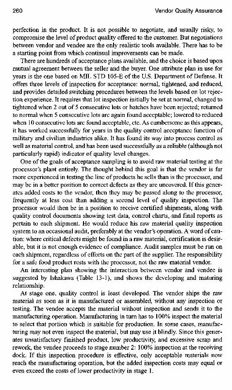
perfection in the product. It is not possible to negotiate, and usually risky, tocompromise the level of product quality offered to the customer. But negotiationsbetween vendor and vendee are the only realistic tools available. There has to bea starting point from which continual improvements can be made.
There are hundreds of acceptance plans available, and the choice is based uponmutual agreement between the seller and the buyer. One attribute plan in use foryears is the one based on MIL STD 105-E of the U.S. Department of Defense. Itoffers three levels of inspection for acceptance: normal, tightened, and reduced,and provides detailed switching procedures between the levels based on lot rejec-tion experience. It requires that lot inspection initially be set at normal, changed totightened when 2 out of 5 consecutive lots or batches have been rejected; returnedto normal when 5 consecutive lots are again found acceptable; lowered to reducedwhen 10 consecutive lots are found acceptable, etc. As cumbersome as this appears,it has worked successfully for years in the quality control acceptance function ofmilitary and civilian industries alike. It has found its way into process control aswell as material control, and has been used successfully as a reliable (although notparticularly rapid) indicator of quality level changes.
One of the goals of acceptance sampling is to avoid raw material testing at theprocessor's plant entirely. The thought behind this goal is that the vendor is farmore experienced in testing the line of products he sells than is the processor, andmay be in a better position to correct defects as they are uncovered. If this gener-ates added costs to the vendor, then they may be passed along to the processor,frequently at less cost than adding a second level of quality inspection. Theprocessor would then be in a position to receive certified shipments, along withquality control documents showing test data, control charts, and final reports aspertain to each shipment. He would reduce his raw material quality inspectionsystem to an occasional audit, preferably at the vendor's operation. A word of cau-tion: where critical defects might be found in a raw material, certification is desir-able, but it is not enough evidence of compliance. Audit samples must be run oneach shipment, regardless of efforts on the part of the supplier. The responsibilityfor a safe food product rests with the processor, not the raw material vendor.
An interesting plan showing the interaction between vendor and vendee issuggested by Ishakawa (Table 13-1), and shows the developing and maturingrelationship.
At stage one, quality control is least developed. The vendor ships the rawmaterial as soon as it is manufactured or assembled, without any inspection ortesting. The vendee accepts the material without inspection and sends it to themanufacturing operation. Manufacturing in turn has to 100% inspect the materialto select that portion which is suitable for production. In some cases, manufac-turing may not even inspect the material, but may use it blindly. Since this gener-ates unsatisfactory finished product, low productivity, and excessive scrap andrework, the vendee proceeds to stage number 2: 100% inspection at the receivingdock. If this inspection procedure is effective, only acceptable materials nowreach the manufacturing operation, but the added inspection costs may equal oreven exceed the costs of lower productivity in stage 1.

Prompted by the volume of returned goods from the vendee's receiving inspec-tion, the vendor now engages in 100% inspection of the finished goods, and thevendee's quality control notes an improvement in the quality of the materialsreceived. As a result, the vendee reduces receiving inspection from 100% to astatistical sampling plan, such as 105-D (stage 4). If he is more confident, and ifthe vendor is willing, the vendee will now be satisfied to merely review the ven-dor's quality control records. Otherwise, the vendee might try reduced inspectionor skip-lot sampling.
The vendor is now encouraged by the reduced costs brought about withrelatively minimal effort at quality control, and expands the coverage (stage 5) toinclude 100% inspection in his own processing department, while reducing thefinished material sampling to an acceptance sampling plan prior to shipment. Thevendee, meanwhile, continues minimal incoming inspection.
Although he may have reached a rewarding level of shipping all satisfactorymaterial, the vendor should explore the possibilities of reducing his own scrapand rework by using some of the tools of experimental design and quality engi-neering. By studying and improving his process capability, the vendor should beable to replace 100% process inspection with process control techniques, whilestill retaining the lot acceptance method of finished goods sampling method forlot acceptance. The vendor has reached stage 6. The vendee continues to checkthe incoming material quality, but may have reached the point where shipments,accompanied by a certificate of analysis, can be accepted.
In stage 7, the effectiveness of process control at the vendor's operation allowsreduction of end-of-the-line sampling inspection and lot acceptance to checking
Table 13-1. Development of Vendor-Vendee Relationship
Vendor
Phase
123
4
5
6
7
8
Manufacturingdept.
100%inspectionProcess control
Process control
Process control
Qualitydept.
100%inspection100%inspectionSamplinginspectionSamplinginspectionCheckinginspectionNo inspection
Vendee
Qualitydept.
100% inspection100% inspection
Sampling orchecking inspectionSampling orchecking inspectionChecking orno inspectionChecking orno inspectionNo inspection
Manufacturingdept.
1 00% inspection
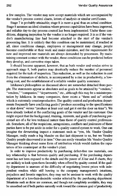
a few samples. The vendee may now accept materials which are accompanied bythe vendor's process control charts, letters of analysis or similar certificates.
Stage 7 is probably attainable; stage 8 is more a goal than an actual condition.Stage 8 assumes an ideal situation where process capabilities have been improved,and reliable day-to-day process control has been implemented. Under these con-ditions, shipping inspection by the vendor is no longer required. It is as if the ven-dor's manufacturing line had become attached to the start of the vendee'sprocessing line. It is unlikely that this condition can be maintained, if reached atall, since conditions change, employees or management may change, peoplebecome comfortable at their work and make mistakes, and the requirements fornew and improved raw materials are always demanded by processors. By main-taining constant contact with the vendor, these conditions can be predicted beforethey develop, and corrective steps taken.
It should become apparent, however, that as both vendor and vendee strive toapproach stage 8, both parties may drastically reduce the number of personnelrequired for the task of inspection. This reduction, as well as the reduction in costfrom the elimination of defects, is accompanied by a rise in productivity, a low-ering cost, and the establishment of a reliable vendor quality assurance.
Ishikawa's philosophies as discussed above are somewhat detached from peo-ple. The statements appear as absolutes and as goals to be attained by "vendors,""vendees," "companies," "departments," etc., although this may be a misinterpre-tation by Ishikawa. In many companies, there exists a "them and us" attitudewhich is extremely counterproductive. The quality control and production depart-ments frequently have conflicting goals ("produce according to the specificationsor shut down" versus "produce at least cost and get it out the door on time"). Wehave already looked at the conflicting goals of the vendor and his customer. Onemight expect that the background, training, interests, and goals of purchasing per-sonnel are of a far less technical nature than those of quality control profession-als. Somehow, all of the suspicions, antagonisms, conflicts and jealousies of theseparties have to be put aside in order for a quality control system to work. One canimagine the devastating impact a statement such as "you, Mr. Vendor QualityManager, really made a big blunder on that last shipment to us, but we VendeeQuality people discovered it in time." One can easily visualize Mr. Vendor QualityManager thinking about some form of retribution which would darken the repu-tation of his counterpart at the vendee's plant.
In order to improve productivity by purchasing defect-free raw materials, onekey relationship is that between quality and purchasing. If the purchasing depart-ment has not been exposed to the details and the power of X-bar and R charts, theyare unlikely to look upon them favorably when offered by quality control. If the qual-ity department is unaware of the difficulty of negotiating lowest prices with inde-pendent vendors while still bowing to the company management's intuitions,prejudices and favorite suppliers, they may not be anxious to work with the qualitydepartment of a less-than-desirable vendor selected by the purchasing department.Situations such as these are common, and though not completely avoidable, they maybe smoothed out if both parties earnestly work toward the common goal of productivity.

SELECTING AND NURTURING A SUPPLIER
The responsibility of vendor selection has historically rested with the purchasingdepartment. Somewhat archaic criteria are still being used in the process: service,reputation, and lowest price. Over the years, selections have been affected to vary-ing degrees by promotional efforts on the part of potential suppliers. Althoughit looks ridiculous in print, decisions have been swayed by friendships, golf, gra-tuities, lunch and dinners. Practices based on these suspect principles continuebecause of the philosophy "if it ain't broke, don't fix it." If quality and productiv-ity is affected adversely by selections based on such decisions, then the suppliersystem is "broke" and needs to be carefully reassessed. Fortunately for both thefood industry and the consumer, these bleak practices are disappearing, and arebeing replaced by far more logical decision-making criteria, with the selectionprocess including input from other concerned department managers.
If the price from a potential vendor appears completely out of line with hiscompetition, it is suggested that before outright rejection, the reasons for thehigher price be investigated. There is always the possibility that the price includesspecial services, higher or more uniform quality, warehousing, delivery conces-sions, etc. Price discussions used to be the first topic of discussion, but are nowmoved further down the line. The first questions should uncover the vendor'scapability to supply precisely those raw materials, ingredients, or packaging sup-plies required by the vendee's specifications on a rigorous delivery schedule.Close cooperation between the two parties may be required in the event that avendor is unable to supply material to the specifications of the processor. In sucha case, it is desirable to have selected a vendor who would willingly develop a sat-isfactory material with the assistance of the vendee. An easily accessible line ofcommunication should be available. The vendor's use of process control and theability to respond to the need for enhancing process capabilities should beexplored. Additionally, he should be able to control the volume of production, andhave the financial ability to insure expansion if required to meet increasingvendee needs.
It is desirable for a vendor to have exhibited a stable management system thatis respected by others in his industry. There should be an understanding of thevendee's management philosophy as well, and close cooperation between man-agements should be established and maintained. The vendor should maintain hightechnical standards and have the capability of dealing with future technologicalinnovations. The vendor must not be in a position where corporate vendee secretswould be breached.
An assessment of the management philosophy of the vendor is closely linkedto the company's quality control policy, and may be difficult to obtain. Person-to-person contacts will eventually disclose knowledge, capabilities, personalities,and quality understanding.
A vendor audit of quality control may be requested by the purchasing depart-ment to reinforce its initial selection of a vendor. Depending on the nature of thematerials under consideration, an initial audit may be extremely detailed, or

somewhat informal. In either case, the following are considered to be necessaryareas for inclusion:
1. The quality philosophy of the vendor.2. Quality records of other (non-competitor) vendees.3. Corporate history and current trends in vendors industry.4. Complete product list.5. Details on equipment, processes, production capabilities.6. The vendor's quality assurance system, including quality education and
implementation programs.7. Vendor's controls on their own procurement of raw materials and
subcontracting.8. Sanitation practices.
Maintaining a good relationship with vendors once they are on line is a nec-essary and frequently rewarding effort. The purchasing department maintains arelationship which may have different objectives than those of the quality depart-ment. The processor's quality records of materials acceptance from each majorsupplier should be routinely analyzed for trends. Nonroutine audits conducted atthe vendor's plant will occasionally disclose practices or conditions which needto be brought to the attention of both the vendor and the processor's purchasingdepartment. If needed, advice and assistance should be freely given to the supplierto eliminate problem areas and to further cement relationships. If indicated, inter-laboratory calibration tests might be run to show an interest in assisting the vendor.A system of rewarding suppliers for implementing and maintaining process con-trols and quality systems will promote effective defect prevention and continuedsatisfactory quality. Because of the mobility of our society, it would not be unlikelyto lose a good vendor-vendee relationship temporarily through loss of key peoplefrom either company. The only choice is to start over again, building up the confi-dence and interchange of ideas necessary to keep the system operating.
Relationships may be improved in many unexpected ways. Suppose that avendor's quality manager has been unsuccessful in convincing his CEO that thereis a need to update laboratory equipment. No more than a word or two from thevendee quality manager to the CEO that his quality laboratory would benefit fromcertain modernized equipment, and chances are the vendor and vendee qualitymanagers become long-term allies.
The terms "vendor" and "vendee" in the above discussion have been usedgenerically. The impression is that they refer only to suppliers and purchasers ofmaterials and products. However, the same principles apply equally to the rela-tionship between processors and co-packers or processors and warehouses. Theco-packers provide an extension to the production lines as a service, and are sub-ject to the same scrutiny and assistance that would normally be provided withinthe processor's plant. By the same token, outside warehouses provide a servicewhich can adversely affect quality unless monitored. Specifically, rotation ofstock or inadequate storage temperature controls may both adversely affect shelf

life. Sanitation, pest control and control of damaged goods are equally criticalquality considerations.
The effect of a JIT (or just-in-time) contract with a vendor raises special qual-ity considerations. Briefly, a JIT system of obtaining raw materials is based ona belief that no inventory of raw materials need be held at the processor's plant ifthe vendor can supply the correct material "just in time" to meet the productionschedule for the day. The system is far from new—it has been in use for years inthe canning industry, for example. Field crops such as corn, peas, tomatoes,peaches, etc. are delivered on a scheduled basis to the canning, dehydrating orfreezing plant within minutes of their actual processing. In spite of the complica-tions which arise in tight scheduling, the system works well, and permits pro-cessing crops at the moment of peak flavor. Similarly, for many years, the can,plastics, glass and paper packaging products manufacturers have supplied theday's packaging requirements to food processors starting on the morning needed,and continuing throughout the production period as scheduled. The savings ininventory storage costs and warehouse space needs at the processing plant areenormous, although in some instances, these needs might simply be moved backto the vendor's manufacturing plants where they generate the costs to be eitherabsorbed or passed along.
Quality control in a JIT system becomes critical. There is no time to reject andreplace a lot of defective incoming packaging materials. They must be producedright the first time. A successfully working quality control system must be inplace at the vendor's manufacturing facilities before a JIT program is started. It isnot uncommon to have a contractual arrangement between vendor and vendee onthe disposition of costs associated with substandard shipments, and there aremany options available. A shipment of substandard cans might be 100% inspectedby the processor, with the added costs absorbed by the vendor. Or the cans mightbe run through the production line and the filled product sorted at the end of theline, with costs of inspection, scrap and rework passed back to the vendor. A post-manufacturing sampling inspection at the vendor's plant prior to shipment mightbe made by the vendor, the processor, or both before shipment is approved, hope-fully eliminating the expensive difficulty of shipping defective materials. In the"real world," either the vendor or the processor or both generally maintain a smallemergency supply of packaging materials to tide them over in the event of a majorquality problem. Whenever a substandard shipment does manage to escape thequality control system, it is imperative that the cause of failure be immediatelydetermined and corrected so that it can never happen again.
Before leaving the subject of vendors, a word or two concerning single sourceof supply would be in order. There has been a growing interest in this concept overthe years. The justifications are that better control of quality and costs can beeffected by the close relationship developed between single source and purchaser;that increased volume sales from the single source should provide quantity dis-counts; that fewer liaison personnel are required from purchasing, engineering,quality control and others; and that a sense of "family loyalty" develops betweenthe two organizations, with better understanding of mutual needs.

On the other hand, the familiarity and friendships which develop between thetwo closely allied companies might lead to occasional difficulty in enforcingunpleasant decisions, such as refusing a shipment on the basis of quality or latedelivery. Other inherent dangers of a single source are those involved in the eventof labor disputes, inclement weather, loss of key personnel, power failures, trans-portation problems, all of which might interfere with continuous on-time deliveryof raw material to the processor. Then there is the ever-present threat of companytakeovers which could spell inconvenience or worse to either of the two compa-nies. In the event that the vendor is bought out, the processor might find itselfwithout a ready source of raw material; in the event of a processor buyout, thevendor might find itself without a customer. The vendor is placed in the uncom-fortable position of depending solely on one major customer, and probably agreatly reduced sales force, since none may be needed under the arrangement. Ifthe vendor is dropped for any reason by the processor, there may not be sufficienttime available to rebuild a sales force to enable it to remain in business. Perhapsthese possibilities can be solved by contractual agreements, but they are potentialproblems to single-source purchasing.
PACKAGING SUPPLIER QUALITY ASSURANCE
Although the following discussion pertains to purchasing of packaging materials,the same principles can be applied to any raw material supplied by an outside ven-dor. The buyer-seller relationship of the past has occasionally been antagonistic.Worse still, the "friendly arrangements" between purchasing managers and someof their vendors were occasionally responsible for the questionable suppliesarriving at the receiving dock. Although these battles and special dealings maynever be completely eliminated, there has been a growing trend toward a rela-tionship best defined as "partnering" between supplier and user. It is becomingincreasingly clear that the seller, the purchaser, and the final product user have allbenefited from this honest and open interaction.
An autonomous purchasing manager for packaging materials developed a qualityassurance program with suppliers, which borders on a vendor certification program.Although the procedures put forth are not necessarily recommended, they havebecome fairly common in companies of all sizes, and in many cases are successful.
Contacts with the vendor's sales people have been handled generally by thepurchasing department. This avoids the possibility of creating violations ofcontractual agreements which might not be known by, for example, qualitycontrol, engineering, or production. On the other hand, frequent meetings ofthe purchasing department with members of all other groups within his companyare mandatory, so that improvements, suggestions, and problems can be aired.These may be identified as formal teams, with a rigorous schedule of carefullystructured meetings, or they might be more informal.
Packaging materials are often as important to the quality of food products as arethe other raw materials, and for some food manufacturers, the cost of packaging

materials is second only to labor costs. Substandard packaging material mayresult in lost production time, loss of materials, claims, and customer dissatisfac-tion. In the past, the practice for preventing non-conforming materials fromreaching the customer consisted of receiving inspection and tests, with the hopethat any defective material would be detected before reaching the production line.Manufacturers have become increasingly aware of the weakness of this system. Itis rarely economically possible to sample every lot of every packaging materialreceived fast enough and reliably enough to prevent operational problems.Furthermore, as production facilities become increasingly automated, there arefewer operators on the line to detect substandard packaging materials which wentundetected at receiving inspection.
The simple solution is to expect improved processes at the vendor facilities.The first step in this conversion of policy is the preparation of complete, accuratespecifications so that the vendor has a clear understanding of the nature of"defective material." The vendor now knows what quality control testing isrequired for his customer, and should be able to provide satisfactory shipmentswith supporting data. In effect, this shifts the inspection and approval of packag-ing material from the processor's receiving dock back to the supplier.Certification papers (if required) include production data, size and frequency ofsamples, test results, and signed reports. Depending on experience with thevendor and the nature of the operation, some companies prefer advanced certifi-cation; others might accept certification with the shipment. Some of the respon-sibility continues to rest with the purchaser, and all shipments should still besubject to audit by them.
In order for specifications to be workable, they should clearly list minimum,and maximum measurements, as well as targets. They should be worked outthrough cooperation with vendors and purchaser jointly. In some instances, thevendor's process capability charts will provide realistic data which both partiesfind reasonable. Most packaging specifications can be constructed as fast as theycan be typed into a computer. However, there are instances where critical per-formance or intricate design will call for patience and understanding between thetwo parties. The engineering drawing of a pour spout, for example, may appear tobe precisely defined, but tiny deviations from the dimensions shown might pro-duce catastrophic leakage. The vendor might provide modifications or compro-mises which can make the design realistic.
Some of the tests run routinely on paper and fiberboard packaging materialsto avoid problems on the line are: material composition, inside and outsidedimensions, tensile, tear, burst, weight, moisture, smoothness, caliper, moisture,brightness (TAPPI: Technical Association of the Pulp and Paper Industry). Inaddition there are hundreds of specific tests for composite cans (Composite Canand Tube Institute), flexible films (National Flexible Packaging Association),cans, glass, paper and fiber, molded plastics, etc.
Management expects that most directives to install a new company system willbe complied with fairly quickly, and and that the new system will be essentially com-plete when introduced. For example, a system to prevent multiple disbursements of
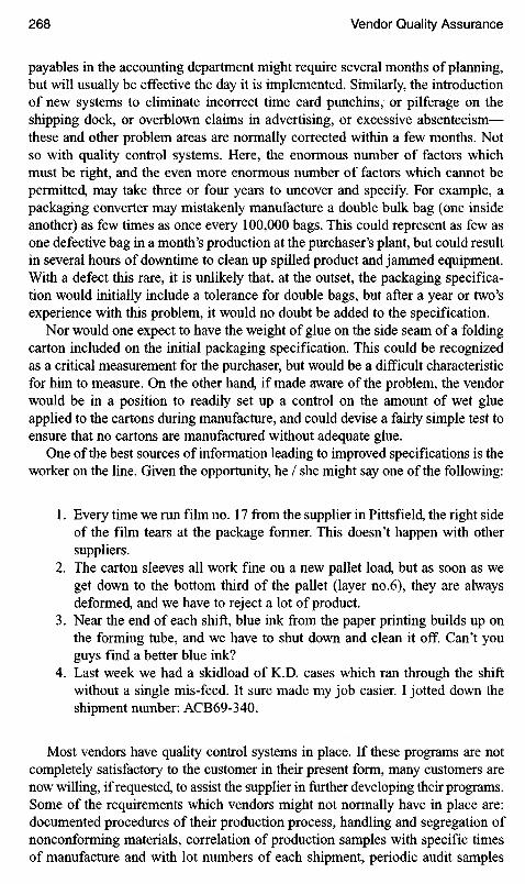
payables in the accounting department might require several months of planning,but will usually be effective the day it is implemented. Similarly, the introductionof new systems to eliminate incorrect time card punchins, or pilferage on theshipping dock, or overblown claims in advertising, or excessive absenteeism—these and other problem areas are normally corrected within a few months. Notso with quality control systems. Here, the enormous number of factors whichmust be right, and the even more enormous number of factors which cannot bepermitted, may take three or four years to uncover and specify. For example, apackaging converter may mistakenly manufacture a double bulk bag (one insideanother) as few times as once every 100,000 bags. This could represent as few asone defective bag in a month's production at the purchaser's plant, but could resultin several hours of downtime to clean up spilled product and jammed equipment.With a defect this rare, it is unlikely that, at the outset, the packaging specifica-tion would initially include a tolerance for double bags, but after a year or two'sexperience with this problem, it would no doubt be added to the specification.
Nor would one expect to have the weight of glue on the side seam of a foldingcarton included on the initial packaging specification. This could be recognizedas a critical measurement for the purchaser, but would be a difficult characteristicfor him to measure. On the other hand, if made aware of the problem, the vendorwould be in a position to readily set up a control on the amount of wet glueapplied to the cartons during manufacture, and could devise a fairly simple test toensure that no cartons are manufactured without adequate glue.
One of the best sources of information leading to improved specifications is theworker on the line. Given the opportunity, he / she might say one of the following:
1. Every time we run film no. 17 from the supplier in Pittsfield, the right sideof the film tears at the package former. This doesn't happen with othersuppliers.
2. The carton sleeves all work fine on a new pallet load, but as soon as weget down to the bottom third of the pallet (layer no.6), they are alwaysdeformed, and we have to reject a lot of product.
3. Near the end of each shift, blue ink from the paper printing builds up onthe forming tube, and we have to shut down and clean it off. Can't youguys find a better blue ink?
4. Last week we had a skidload of K.D. cases which ran through the shiftwithout a single mis-feed. It sure made my job easier. I jotted down theshipment number: ACB69-340.
Most vendors have quality control systems in place. If these programs are notcompletely satisfactory to the customer in their present form, many customers arenow willing, if requested, to assist the supplier in further developing their programs.Some of the requirements which vendors might not normally have in place are:documented procedures of their production process, handling and segregation ofnonconforming materials, correlation of production samples with specific timesof manufacture and with lot numbers of each shipment, periodic audit samples

supplied to customer which duplicate vendor's production samples. On the otherhand, for less critical products, perhaps simple checklists of vendor operationscould be satisfactory documentation for the purchaser. If, for example, the check-lists indicated a number of culling problems throughout a production run, the pur-chaser would also expect to find a series of inspection reports accompanying anyshipment involved, which indicated appropriate culling of defects at the vendor'splant. In the event that this becomes a continuing problem, the vendor would beexpected to provide a more formal quality control system. Where informal check-list systems are used, some purchasers find it desirable to receive the checklistsin advance of the shipment, since they might consider it necessary to have thevendor conduct further defect removal. Formalized quality control documents, onthe other hand, usually accompany shipments.
In examining shipment documentation, it should be apparent that the immensevolume of paper could not reasonably be digested by purchasing, quality control,receiving, production, and engineering. As the program evolves, the record flowshould indicate a road map where certain documents are directed to specificdepartments for review before they are collected at some central office, usually inpurchasing or quality control. As a guide, the paperwork should be reviewed bythe department which needs the information to operate, and by an individual whounderstands how to read and interpret the data. A control chart which shows eightpoints all in a row with the same value might be interpreted by the untrainedreviewer as an example of superb process control. In fact, it might indicate thatsomebody was falsifying test measurements.
Even under the best quality control systems, it is possible that over a longperiod of time, as many as three shipments per thousand might possibly be sub-standard. Here is where the huge data file is most valuable. By careful detectivework, it is frequently possible to pinpoint the cause of the reject. In some cases,the problem might not be observed in every portion of the shipment, but might beisolated to the left side of machine #9 during the last half of the second shift onnearly every Tuesday (for example). With detailed supplier data such as this,process improvements may be indicated, and specific products can be culled fromthe offending shipment, rather then outright reject-and-destroy. Costs involved inthis inspection are usually negotiated amicably.
The question arises: who should be responsible for holding a shipment whichis accompanied by questionable data? Or, for that matter, who should be respon-sible for rejecting an incoming shipment when either the data or an audit showsit to be unsuitable? Also, who, if anyone, should have the authority to override ashipment rejection? There is no single answer to these three questions, and yet,they are critical to the control process. Each company finds its own workablesolution, depending in part on the function of the departments involved and, to alarger extent, on the abilities of individuals within each company. Where qualitycontrol, purchasing and operations are all equally capable of handling thedecision unilaterally, it might be preferable to appoint one department to handlesimple, routine rejections or approvals, and to construct a small team consistingof the three departments to act as a material review board. Needless to say: thesimpler the better! Obviously, this works best in relatively small organizations.

Carried to an extreme, there is a point at which too much record keeping canevolve from a relatively simple system of reporting. If the vendor is a paper con-verter, should he also supply documentation from all of his suppliers? The papermill would normally provide documentation with each shipment; the other rawmaterial companies might supply theirs: ink, staple wire, coatings, glues, metalstampings, etc. Perhaps a statement from the converter which indicates that he hasinspected all of these materials and found them within their specifications shouldsuffice. There may be instances where the customer might wish for copies of out-of-specification sample test results, along with the specific causes, and informa-tion on steps taken by the vendor to correct the process.
Occasionally the customer will find the need to modify an existing specifica-tion, or perhaps create an entirely new specification to accommodate a process,product or packaging change. These changes require close cooperation betweenvendor and customer well in advance of the contemplated production. Agreementshould be reached on quality control basics: sampling location, size, frequency,methods of test and reporting. Advance samples from the vendor should be subjectto both laboratory audit and production pretest well in advance of the scheduledfull production date.
Close relationships with the vendors processes and quality systems can lead toan occasional ethical dilemma. If a vendor should experience a quality problemwhich requires considerable time and expense to correct, does the purchaser havethe right to pass this information on to competitive vendors? Although this mightappear to be unfair, there is a workable solution that some manufacturers havefound to be acceptable. During the early discussions of closer working relationshipsbetween vendor and purchaser, this subject of sharing proprietary information withother vendors needs to be explored in detail. Most vendors will accept the idea, withthe understanding that by sharing their own efforts with other vendors, they mayhave as much to gain in return. If a vendor wishes to exempt specific areas oftrade secrets from this agreement, it should probably be expressed in writing.
The "partnering" concept of the vendor-purchaser relationship tends to leadtoward the single source principle. As a supplier and the purchaser grow closertogether over time, understanding needs and capabilities, the purchaser mightcome to treat the supplier as part of his company—a partner. With this close inter-change, the purchaser might well decide that there is no need for a second or thirdsource. On the other hand, there is no one best way to manufacture corrugatedshipping cases. Each supplier of corrugated has developed his own productiontechniques with his own specialized equipment, and has, over the years, discov-ered solutions to countless production problems, many of which are unknown tohis competitors. This is one of the compelling reasons why so many purchasingmanagers prefer two or three sources.
Record Keeping
Quality documents pertaining to shipments should be accumulated by eitherpurchase order number or shipment number. In addition, vendors should supply

calibration information related to their test equipment and reagents. By usingavailable computer tools, the paperwork can be kept to a minimum. For example,scanner outputs, fax-modems, floppy disks and CDs containing data can be trans-ferred electronically to a central filing system with minimum effort, and keyed toshipment numbers.
The use of specialized universal product coding, in addition to the productUPC information which appears on shipping cases (for example), can be tailoredto fit specific needs of both vendor and purchaser.
The major contribution to the partnership concept of quality control betweenthe packaging material vendor and purchaser was expected to be a combinationof reduction in defects on the processor's production line, as well as lower costsof purchased materials by elimination of manufacturing interruptions at the ven-dor's plants. A greater benefit has been the ability of the processor to adopt a"Just-In-Time" delivery schedule for purchased materials. As the defect level ofincoming materials disappears, it is no longer necessary to maintain high levelsof backup stock on the warehouse floor. As one pundit described this change: wehave replaced "Just-ln-Case" production with "Just-In-Time." Eliminating theneed for this cushion of materials also frees up a significant amount of capital.Obviously, for those with uncertain delivery operations resulting from occasionalsevere weather, unpredictable harvest conditions, unscheduled labor conflicts,extremely long supply routes or other traffic problems, "Just-In-Time" cannot betaken too literally. Allowances must be made for these extraordinary circum-stances.
A note of caution: this approach appears to depend on one purchasing man-ager and one supplier sales representative. Although this system can be quiteeffective, the danger of losing either of these individuals through promotion orotherwise might severely handicap the business relationship and effectiveness.
SUPPLIER CERTIFICATION PROGRAMS
In much of the above discussion, the word "certified" has been used to describea guarantee of product quality or a recognition of a supplier's quality qualifica-tions. The USDA has offered a certifying service for many years. Since the 1970s,the United States Department of Agriculture has furnished an inspection servicewhich provides certification of food processing plants and the quality ofprocessed fruits and vegetables, honey, molasses, nuts, sugar, sirups, tea, coffee,spices and condiments. The regulation is found in USDA CFR TITLE 7, Chapter 38Food Safety and Quality Service, Part 2852. Plant certification requires a plantsurvey by the USDA to determine whether the plant and methods used are suit-able in accordance with their regulations, as well as those of the FDA GoodManufacturing Practice in manufacturing, processing, packing or holding. If theplant meets the requirements of the survey, product inspection services may beperformed. Certificates of sampling and loading are issued. Official grade stampsare affixed to those lots packed under either continuous inspection of the USDA

or packed under the Quality Assurance Program of the USDA. Additional detailsof the regulations, including sampling plans and acceptance levels have been pub-lished in a manual titled Regulations Governing Inspection and Certification ofProcessed Fruits and Vegetables and Related Products, USDA, Food Safety andQuality Service, Fruit and Vegetable Quality Division, Processed ProductsBranch, Publication 0-310-944/FSQS-378.
Many companies have customized certification procedures as part of theirtotal quality management (TQM), in contrast to the packaging purchasing man-ager's example discussed above.. These programs appear under such other titlesas Supplier Improvement, Vendor Partnership, Supplier Qualification, PreferredSupplier, Supplier Development, Vendor Excellence, Supplier QualityManagement, Select Supplier. By spreading the responsibilities and goals overmany company departments, the shortcomings of the packaging materials exam-ple above are reduced. Some food companies will certify suppliers without auditprovided that they have been inspected by recognized external organizations suchas the American Institute of Baking, or by qualified food industry consultants, orhave become ISO 9000 certified. This is certainly a short cut to certification,since large companies have reported that it can require three to five years toachieve fully qualified approval. Some of the vendor's major quality control areaswhich are examined by various companies include:
Continuous improvementData managementExperimental design techniquesFault tree analysisGood Manufacturing PracticeHazard Analysis and Critical Control PointsKosher certificationLaboratory capabilitiesOn-time delivery systemContamination controlProcess capability studiesProcess controlQC audit systemRecall proceduresRecord retention systemSampling proceduresSample retention systemSanitation—macro and microSpecificationsTest methods—accuracy and precisionTraceabilityTraining programs
In the simplest form of a supplier certification program, the quality controlmanager prepares a questionnaire for the potential vendor, listing titles of qualitycontrol procedures considered essential to providing satisfactory materials to

his company. The questionnaire is filled out by the vendor and returned to thecompany's purchasing department where a decision is made to "certify" whetherthe vendor is acceptable.
Another simplified system requires that each vendor's shipment be accompa-nied by a quality certificate, with or without supporting test data and controlcharts demonstrating compliance with specifications. These certified shipmentsmay be audited by the purchaser's quality control department.
Although these simplified methods appear somewhat elementary, they may besatisfactory where the products involved are ordinary and uncomplicated. Insome cases they may also be all that a potential supplier will tolerate from a smalllot buyer.
At an intermediate level of program sophistication, some customers willconduct plant visits to rate potential suppliers on several specific criteria beforecertifying them: statistical quality control procedures, product quality, processcapability, service, and price. Selecting the initial candidates for certification isusually based on the dollar value, critical nature of the product, volume of mate-rial supplied, or perhaps single source suppliers. Generic product suppliers (salt,oils, sugar, corn syrup, simple maintenance parts for machinery) can be includedafter the critical product suppliers are in the program. These plant visits can bemost fruitful if the supplier receives a clear understanding of how his product isto be used. They may provide suggestions to improve the use and decrease thecost of their product.
Larger companies have developed more detailed programs. More than onecompany has formed a team to visit the supplier's plant to directly review theroutine quality control procedures as well as the quality control tools in use fortrouble shooting and product improvement. The team is composed of membersfrom purchasing, production, and quality control, and starts its investigation withthe vendor's top management. If indicated, the team may request that he attend aseminar on total quality management. Obviously, this last step must be accom-plished with much tact and good judgment.
The common goal of the certified supplier programs is the assurance of receiv-ing problem-free materials or services on time, all the time. Some companies willcontribute to this goal by providing technical assistance to the supplier forinstalling quality control systems. A second common goal is to reduce cost. Thiscan be accomplished by reducing losses from defective materials, from eliminat-ing receiving inspection and returned shipments, and from supplier processimprovements, possibly aided in part by the purchaser's technical personnel. Athird goal is to improve the quality level of the product purchased throughimproved operations by the supplier. A fourth goal expressed by a few companiesis to develop a virtual partnership between vendor and purchaser to their mutualadvantage. With the exception of the USDA program mentioned above, pur-chasers will generally certify specific products, not the vendor's complete line ofproducts or entire operation.
The most complete formal programs, generally in large companies, are some-times considered proprietary, and nondisclosure agreements must be signed.

These programs generally include stages of certification which demonstrate thata supplier has furnished product or service which:
Consistently reaches an established quality levelComplies with all governmental regulationsMeets Just-in-Time requirementsContinually improves product qualityImproves price / value relationship
Approvals generally are accomplished in three to five stages (or more), andsuppliers may be identified by a number of classifications, as shown in the fol-lowing table:
Stage
I.
II.
III.
IV.V.
Vl.
Classification
PotentialRestrictedProvisionalLimited
ConditionalAuthorized
AcceptableApprovedAccredited
QualifiedSelectCertified
Continuous
Suggested Descriptions
Might become a supplier after product orservice has been sampled and reviewed
May furnish products on limited basis, subjectto receiving inspection
Preceded by plant visitCertificate of analysis requiredSelected to participate in certification process
Delivers consistent, excellent quality PreferredMeets all of the TQM process, product andservice requirements
Periodic audits of plant and product
As complex as these certification programs appear to be, there is increasingevidence that they are effective in both cost savings and quality improvements. Itis expected that this business technique will continue to grow in popularity.

14 Implementing aQuality ControlProgram
MANAGEMENT COMMITMENT
When top management directs that a quality program be created and adhered to,the quality manager's job is relatively straightforward. He arranges for staff andsets about organizing a system starting with specifications, manual, methods ofsampling, testing, reporting, auditing, methods improvement, cost reduction, andtraining. Usually the first efforts are centered around production. Assuming initialsuccess and also assuming that the directive is still in force, the next logical step isto install quality control programs in other departments within the company: ship-ping, purchasing, accounting, sales, marketing, personnel, engineering, etc.
The chances are that this is not exactly what top management had in mind. Priorto the 1940s, quality control meant "inspect the raw materials and the finishedproduct, and don't let anything bad get by." There are still organizations with thisattitude, and there may even be some where the product and process is so simple,and the employees so dedicated to high quality production, that it may work satis-factorily. For some older food companies, the main goal for years has been to getas many cases of product as possible out the door, and using quality control toassist production to attain this goal would be acceptable to company personnel; butquality control should not be allowed to "waste their time" in other departments.
The concept of total quality control, that is, quality control encompassing allof the company's functions, is still fairly new. It is often difficult to install becauseof the closely-guarded-turf syndrome: "I'm the accounts payable departmentmanager, and nobody from quality control or anywhere else is going to tell mehow to run my business." Yet, the quality of work in the accounts payable depart-ment may be very poor. Payments may be so slow that thousands of dollars ofprompt-pay discounts are lost; X% of the checks may be sent out with the wrongamount, to the wrong account, or duplicated. Y% of the invoices may be misfiledor destroyed. Z% of the invoices may be for unsatisfactory services or perhapsthose not performed at all. Certainly, the statistical quality control principlesusing sampling plans and statistical analysis can be used to pinpoint weaknesses
in the system, and provide measuring devices for process improvements.It would not be unexpected for the accounts payable manager to tell the qualitycontrol manager, "Don't try to educate me with your quality control principlesuntil you've solved all the problems of poor product quality control on theproduction line. That's what you were hired for." And in many cases, he could beright!
With this in mind, we will restrict our discussion of implementing a qualitycontrol system to those areas of a food processing company directly involved withoperations.
GETTING STARTED
To begin with a more optimistic note, a statistical quality control program can becreated in a company with or without the direct support of top management.Support merely makes the job easier. If management has selected a philosophysuch as statistical or motivational, the first step has already been taken; and fromthere on, every step should refer to that philosophy.
It is possible to buy books, video tapes, or consultant services which supplypreformed quality control programs prepared for other companies. Some of thesemight be applicable, but one must recognize that although the principles mightwork for all, the details may not fit into the product safety, the cultural atmos-phere, the product line, the governmental regulations or the physical processingequipment of every company. Trying to educate managers in a darkened roomwith video tapes aimed at another type of industry will likely put some of them tosleep. A program aimed at certain hardware industries may be built around suchprinciples as "reliability," "mean time between failure," and "warranty control."Much of this does not apply to food products. The quality control program of afood product cannot be built around a concept that even suggests that the food'sreliability makes it safe to eat 87% of the time; or that if it should produce sick-ness it may be returned for "repair" under a warranty certificate. Some of the pro-grams have zero defects as a goal. In reality, the only way to reach zero defects isto widen the specifications. As soon as the line worker realizes this, the programloses its punch. This does not mean that there is no value in a zero defects goal.It is an admirable way to present progress charts. Where attribute acceptance pro-grams are used, an improvement in quality control which permits dropping theacceptable quality level (AQL) to the next more stringent table—closer to zero—should be heralded with loud applause throughout a company bent on improvingthe quality level.
Avoiding blind acceptance of hardware or electronic quality control programscannot be emphasized enough. In an article published in Quality Magazine(November 1988, p. 20), a production manager of Hewlett-Packard Co., the world'scurrent leading test and measuring equipment manufacturer, admitted to a majorproblem with product quality. The article describes how, in 1981, there was a 50%chance of product failure resulting in the equipment being returned for warranty

repairs "within certain areas of the company." By instituting a new stringentquality control program, the annualized failure rate was reduced stepwise so thatby 1985 the failure rate had dropped to 14%. After a few swings in either direc-tion, the product failure rate leveled off at 4% by 1989. The target failure rate forthe 1990s was estimated to reach about 3% to 4%. Certainly, a quality control pro-gram such as this one, which has been claimed a huge success for a company inthe electronics industry, cannot be used without some major modifications in thefood industry. In the first place, it is inconceivable that a food product with a 50%failure rate would ever be considered ready to market. Furthermore, there is no"repair under warranty" concept for the food industry's consumers. Finally, thethought of a 3% failure rate as a goal for a food product is ridiculous. If 3% of car-bonated soft drink cans were failures (leaking cans permitting the carbon dioxideto escape, pull tab openers which fell off when attempting to open the can, productcontaminated with cleaning fluids, jagged edges on the pour opening, moldyproduct, wrong flavor, missing formula ingredients such as acid, color or flavor-ing), then one of every 17 six-pack cases sold would result in a dissatisfiedcustomer. This is totally unacceptable for any food product.
Some programs are aimed at quality control personnel and tend to be highlymathematical. If presented in digestible doses to those personnel, they may betrained quickly and efficiently. On the other hand, a mathematics based program,loaded with statistical terms and dull tables, will not readily be embraced bymost managers or supervisors whose backgrounds make this material difficultto absorb. The lesson to be learned here is that any potential program shouldbe screened before presentation, and if not applicable to the company, anotherprogram must be found or created.
AN IN-HOUSE PROGRAM
One major food processor tried such a formal mathematical program and foundthat it was poorly received. They then attempted to put together small teams ofoperations and line personnel at which cost savings projects were discussed andat which fragments of statistical training programs were taught. This approachworked. With specific company goals to keep their interest, the teams almostimmediately introduced methods modifications for product improvement andcost savings. At the same time, they were made aware of the meaning of statisti-cal control in a relatively painless fashion, so that when they encountered X-barand R charts on the plant floor, they were familiar with their meaning. Asexpected, an effort of this type must be closely monitored since it will, by its ownnature, generate costs: lost time, lost labor, lost production.
These teams were not modeled after Japanese quality circles. The teams con-sisted of management, supervisory, and hourly personnel, and the discussions wereguided along specific problems. This gave everybody an opportunity for inputwithout wasting time with unsound engineering approaches to complicated sys-tems. In order to start a team in the right direction and to show how team efforts

are effective, a simple demonstration was conducted. In this example, a teamleader went through the preparation of a peanut butter sandwich, but without plans,tools, or materials readily available. He crisscrossed the front of the room lookingfirst for the bread, then a plate, then a knife, and then the peanut butter. He stoppedto perform other actions which had no bearing on the project, such as getting adrink of water, stopping to open up a pack of chewing gum, and looking fora wastebasket for the wrapper. After ten minutes of aimless and uncoordinatedmotions, the peanut butter sandwich was finished. Following this, a single mem-ber of the team was asked to list all the wrong actions and suggest correct meth-ods to perform this simple task efficiently. This was followed with a teamdiscussion to demonstrate how many additional and better ideas could be gener-ated by group contributions. After a few days of practice with actual productionline situations, the team came up with a few minor productive suggestions relatingto their job. The individuals gradually realized that their input was being used, andemployees at all levels were gratified to be considered a part of the productionteam. As they became aware of the positive results, some of the more technical andstatistical information from the Juran and Deming principles was slowly intro-duced. Under these conditions, the teams were more receptive to statistics, andthe education program was under way.
The next stage was to introduce outside professional training. Some of theemployees were sent to community college statistical quality control courses. Inaddition, a private consultant was brought into the plant to conduct a series ofcourses to groups of employees who were now partly pretrained and ready for theheavier material. Several quality control employees were also selected for spe-cialized five-day training in process control courses by the consultant. These spe-cially trained personnel then presented four-hour classes each day over a periodof three days to the production personnel in the plant. Rather than presentingdetailed procedures, these courses included sound statistical principles as anoverview, covering much of the subject matter contained in this book, but onsomewhat of a theoretical approach: sampling, distributions, control charts forvariables and attributes, data collection, and chart analysis. This endeavor turnedout to be only partially successful. It was too general and theoretical, and failedto give the plant people the specific tools they needed. Management looked at thispart of the program as "planting more seeds" of statistical quality control, withthe expectation that if enough seeds were planted, sooner or later somethingwould sprout.
At the outset, the production managers and the plant managers were invited tothese consultant lectures as well, but they did not choose to attend. This wasunfortunate, for the hourly plant people read this not only as a lack of intereston the part of the managers, but as an indication that they probably didn't believe inthe idea of quality control. Unless the workers are assured that the manager thinksthe program is important, the workers will not pay much attention at the classes.
One of the earliest statistical tools presented by this same company to lineworkers was Pareto analysis. It was offered at first as a dollar-saving tool. Half-hour sessions one day per week were scheduled for the team to teach them this

technique, and eventually apply it. Pareto analysis is simple to present and under-stand, and it was shown to be powerful. The company which tried this approachis a large food processor, with plants nationwide. When the program was started,six teams were assembled, and due to their successes, their number was expandedto over 100 within four years. The 100 teams were credited with generating over7 million dollars of saving a year. Although the program was originally under thedirection of the quality control department, it grew to a point where it had to betransferred as a separate ongoing operations department function.
This company feels that it still has a long way to go before it considers thetraining program a complete success, but the progress has been steady, and in fouryears the spirit of cooperation has spread out more and more through all depart-ments. There are still some supervisors who greet suggestions from the qualitycontrol technician with, "Fm busy; stop bringing your problems to me." Pressureapplied indirectly from the technician to the quality control manager to the plantmanager, and down through the various layers to the uncooperative supervisor,usually results in grudging compliance. In time, this supervisor will realize thatthe suggestions are of value in improving his department's productivity, and even-tually cooperation will be easier to obtain.
As a matter of interest, this company used to depend upon a suggestion pro-gram to generate new cost-saving ideas. Employees who contributed successfulprograms were compensated for their ideas. That program has been all but aban-doned as unsuccessful. The most serious problem with the suggestion programwas its bureaucratic nature. A suggestion from a worker could take months towork its way up through levels of management and, if approved, more monthsback down again before any action could be taken. To add to the failure of the sys-tem, some of the approved ideas, for which the employees were rewarded, neverwere implemented. The new team programs also have a compensation and awardsplan built in. Successful teams receive a cash award at the end of the year, calcu-lated as a percent of the savings actually generated. Occasional interim awards inthe form of gifts, jackets, pen sets, etc. are presented at special dinners or sportsevents. These presentations are made by senior members of the firm, usually vicepresidents, to impress on the teams their importance to the company.
TEAM QUALITY SYSTEMS
The preceding examples of team development and operation are each based onrelatively unstructured beginnings, evolving into formal team programs after theirusefulness has been demonstrated. Over the years, universities and consultingfirms have refined systems for team structure, training and operation which havehad successful implementations. It is unlikely that agreement will be reached onthe "one best method" of introducing teams because of the wide differences inmanagements, culture and diversity within industries.
Team activities are performed in a wide variety of ways in food companies.Although often thought of as modified quality circles, the concept is not new.

In November 1932 McCormick and Company established a team known as the"Junior Board." They met periodically to discuss improvements in operations, andreported their suggestions to the senior board for action at their next meeting.During the first five years of their operation, over 2000 suggestions were acceptedand implemented, with resulting improvements in plant production estimatedat 30%. The specific methods of composition, operation and compensationhave changed over the years, but the overall concept remains.
Articles in food trade magazines and newspapers report a steady stream of suc-cessful team projects in a wide variety of areas: new production techniques, refin-ing accounting procedures, moving facilities to less expensive locations,absenteeism, accident reduction, processing customers' orders, reduction in linechangeover time, defect reduction, material ordering practices, improve sanitation,reduce energy consumption, reducing breakage, customer-driven product specifi-cations, improved stock rotation, community-plant relations, on-time delivery.
The team approach to improvements and problem solving may not work foreveryone. Some of history's product and system inventive geniuses probablyworked best without a team of "equals." Thomas Edison, Albert Einstein and LutherBurbank are examples. Where a company is fortunate enough to employ somenear-geniuses, perhaps it would be best to allow them to work alone, if that isthere expressed need. And there are many formalized team organizations directedby an autocratic coach, who cannot (and perhaps should not) encourage or acceptempowerment of their individual members: sports teams such as football, base-ball, basketball, soccer and hockey come to mind. The same is true of symphonyorchestras, where the will of the conductor may not be challenged withoutdestroying the unified perfection of the ensemble.
A quality improvement team cannot be expected to replace a quality controlsystem. On the other hand, it is unrealistic to expect any single employee to havethe ability to solve all quality and productivity problems, and provide a flow ofimproved quality and productivity ideas. Thoughtfully selected and trainedemployee teams can contribute to improvement in every company's operation andprofitability. Note the wide variations in quality team operations:
1. Team sizes. These vary widely according to complexity of the projectand the needs perceived by management—there are no rules for mini-mums, but it is wise to limit the size to avoid interminable discussionswithout conclusions. (A major candy company found an exception to thislimitation: at one point in the development of a new candy product, theyclaimed to have had 150 people working on the project.)
2. Leaders. It is possible to have successful teams without leaders, butchances for direct action are improved with the appointment of a leader,either by management appointment or by team election. Some teams seemto work well with revolving leadership.
3. Team assignments. For greatest opportunities, these are often presentedin general terms to allow for open-minded exploration of the entire subjectby the team. More frequently than not, the final problem statement turns

out to be quite different than originally thought by management, and mayresult in more far-reaching quality improvements and cost-saving results.
4. Rewards. There is little agreement on the methods for rewarding teamsfor their successes, in part because of the possibility of fomenting teamjealousies, and partly because of perceived uneven-handed recognitionof groups over individual efforts. Agreement by labor unions to a rewardplan has been a problem for some. The Human Resources Department isfaced with a decision on whether to reward individuals as determined byclassical evaluation methods, or to review the individual's performance ingroup activities.
5. Schedules. Different teams within the same company might have varyingmeeting schedules depending on complexity of the project, technical abil-ity of the members, and availability of both company and outside informa-tion. In addition, the urgency of the project will influence the schedule.
It would appear from this discussion that quality improvement teams are allunique, but successful teams do have six things in common: management sup-port, training in quality team techniques, a stated mission, interdepartmentalmembership, budgeted funds, and empowerment.
Just as quality improvement teams require input from various departments, theResearch and Development Department's efforts eventually involve other depart-ments before introduction of a new product. Many companies have formalized theprocedure by creating cross-functional R&D teams. Initial ideas for productresearch may originate in the marketing department, or from a customer, or fromany employee's interesting idea. An R&D team will receive input from marketingregarding pricing, packaging, portion size, and other product specifics.Production, engineering and quality control provide information regarding spec-ifications, test requirements, equipment and procedure needs. Purchasing locatesand prices ingredients and packaging materials. Cost accounting calculates pro-totype standard costs, and determines pricing. Outside sources of informationmay come from equipment manufacturers, customers, raw material suppliers, andthe advertising agency.
There are many sources of detailed information on various types of team oper-ations. Figure 14-1 illustrates four concepts of team formation. Type IV is aninformal and ineffective choice, selected by management which is not particularlyserious about the use of teams. Type III is a step in the right direction, where amanager realizes his shortcomings and solicits assistance from other departmentsto act as an informal team. Type II is a fairly effective method of team formation,and has been used to solve specific production or quality problems. Type I teamshave the greatest potential for continued success.
Some authorities have segregated teams into various classifications, depend-ing upon their longevity and scope. Examples are: (1) the project team, which isassembled with a single specific goal in mind, and usually consists of a smallgroup of employees who are all familiar with the problem or system to beexplored; (2) the permanent team, generally appointed by management to meet on

IManagement forms a team which represents every department. The goals areproblem solving, process and quality improvement. Training is furnished to all.
IlA team is formed from several experienced workers in the affected departmentswho are directly involved with a specific problem. They are likely to cooperate inmaking it work, since they have a personal commitment to suggested solutions.
IllA department head has no training or experience in the financial or engineeringskills (for example) required to solve a quality improvement problem. He assem-bles members of the financial and engineering departments to form a teamwhich should fill in the voids of his qualifications.
IVNobody in management has a solution to a new quality problem. A team of man-agement friends meets to look for useful ideas.
Figure 14-1. Team formation concepts.
a prescribed schedule, and to consider opportunities within a specific area, orgroup of areas; (3) the self-directed work team, which is empowered to considerany and all aspects of an organizations processes.
Once a plan has been formalized for team selection, the next step is training. Forsome quality improvement teams, it may be advantageous to teach the basics of con-trol charts and elementary statistics; for others, this need can best be performed byexperts in the company, or contracted from outside consulting services. In addi-tion to providing guidance on principles of cooperation and ground rules for con-ducting work sessions, a number of techniques need to be taught to the members:
• Brainstorming• Process flow diagramming• Fishbone chart construction and analysis• Pareto analysis• Scatter diagram preparation and interpretation.
Finally, the Deming cycle: PLAN/DO/CHECK/ACT (also referred to as theTQC improvement cycle, or the PDCA cycle) must be understood by all membersso that the proposals of the team can be finalized. Team recommendations in thefood industry may require an extra step to assure that the end product complieswith governmental regulations and safety standards.
STEPWISE PROCEDURES FORTEAM PROBLEM SOLVING
After the initial training programs for the various teams are well underway, eachteam is presented with a practical problem in its production area. Rather than

attempt to solve a major problem at the outset, it is broken down into small proj-ects which can be more easily handled. To make the project easier to understand,it is then shown to the team as a fishbone diagram. The problem causes are foundby team brainstorming, and placed on the diagram. The next logical step is to ana-lyze the importance of each of the potential causes by use of a Pareto analysis. Itis worthwhile to spend the time starting with a numerical Pareto analysis, and thenfollow it with a dollar analysis, since the most frequently appearing problem maynot be the most costly. This now gives the team a series of project priorities basedon the value to the company.
Once the major problem has been selected, the process is studied in detail. Thetools generally used for this are the process flow chart and the process flow dia-gram. At this point, the team is ready to brainstorm for possible solutions to theproblem. The rules for brainstorming are simple: a facilitator or leader is chosento maintain order. The facilitator asks for suggestions at each point on the fishbonediagram, and the team offers "brainstorm" thoughts in rotation, one team mem-ber at a time. All thoughts are written on a blackboard. From this point, the teamproceeds to data collection.
The three main reasons to collect valid data are discussed by the team, withrespect to the problem at hand:
1. Analyze the process to determine its capabilities and limitations, with thegoals of improving the capabilities and eliminating defects.
2. Provide the basis for action to achieve a state of statistical control over theprocess.
3. Inspect parts or products for inspection or rejection.
It should be emphasized that collecting data when the solution to a problem isnot fully understood should be aimed at "exploring," not "proving." Thorough studyof the data should be undertaken with all of the tools available: frequency distribu-tions, histograms, and line charts. As a training aid, a Quincunx might be introducedat this point to demonstrate the generation of normal distributions through randommotions of beads fed first at one target, and subsequently at another. This demon-stration should lead into an explanation of three-sigma process control. The theoryis followed by fitting the data collected on the plant floor to a normal curve, and cal-culating the control limits. Finally, the data is plotted on Jf-bar, R charts to furthersimplify discussion of the process. By the time the team instruction has reachedthis point, the members should have a fairly clear concept of problem solving andthe tools of quality control.
The procedures for corrective action are introduced. Finally, the quality con-trol reporting formats are presented and explained. For one particular company,the quality control manager prepares daily summary reports which are discussedat staff meetings. The major report is one page of HACCP summaries, pie chartsshowing defect causes, Pareto charts which highlight major problems, and con-trol charts for plant operations. These reports can be prepared by hand, but aremore commonly computer generated. Teams then review quality control recap

reports which are much more detailed, and include summaries of all team proj-ects. The recap reports form the basis for management decisions on the schedul-ing of future team projects, as well as decisions to install new equipment, newprocedures, or new processes to implement team suggestions.
This completes the first cycle of team training, problem discovery, problemanalysis, data collection and analysis, proposals for problem solutions, review andimplementation—and then on to another problem discovery and solution.
An example of a cost-improvement project is found in maraschino cherryprocessing.
Operation: Raw -» Bleach —» Color —> Flavor —> GlassCost per pound: $0.40 $0.70 $1.00 $2.00
Historically, a plant had stationed four inspectors at the raw cherry-receivingtables to remove blemished, crushed, and spotted cherries. An additional eightinspectors were stationed along the bleach discharge belt to pick out defectiveswhich had passed the first table. The reasoning behind the double-sized crew wasthat the bleached fruit showed up blemishes more clearly than the red-colored fruitat receiving. Finally, three inspectors were distributed between the color and glassoperations. One of the improvement teams asked the logical question: "Would it notbe more profitable to place most of the inspectors at the beginning of the line wherethe defects that would be discarded were worth only $0.40 per pound, as contrastedwith throwing away defects after coloring which were worth $1.00 a pound?" Theobvious "yes" answer leaves some doubt as to the effect this would have on finalquality. No amount of discussion would resolve the question without hard data tosupport it. A series of tests was conducted with various numbers of inspectors atvarious locations, using statistically designed experiments. The final results showedthat two inspectors were still needed after the color operation, and that only10 inspectors stationed at the receiving tables could produce satisfactory productquality, thus saving two inspectors and thousands of dollars needlessly spent onbleaching and coloring defective material which would subsequently be scrapped.(From a practical standpoint, the savings, though substantial, were less than expectedbecause markets existed for flawed product, although at substantially lower prices.)
PROGRAMS WITHOUT MANAGEMENT SUPPORT
The program described above was blessed with top management support, and wasspearheaded by a dynamic quality control manager who made it work success-fully. But what happens to the team effort if this dynamic manager moves on toanother company? If he is replaced by an equally competent leader, the programwill continue as long as it receives continued support. If, on the other hand, noleader appears, it is possible that each team will become autonomous, and effec-tiveness is bound to suffer. When everybody is in charge, nobody is responsible.The teams will crumble.
Another ugly possibility is the loss of support due to a change of heart on thepart of the chief executive, or worse still, a change of the chief executive to onewho has other priorities. Changes are not merely possible- they are likely. Topmanagements do change from time to time, and the possibility of a merger bring-ing in a new quality philosophy is not unheard of. An equally unpleasant scenario,and one which may be fairly common, is the directive by the new chief executiveto the quality control manager: "Here's $100,000. Go build a quality controldepartment."
Under any of these conditions where top support is not available, the tendencyof a new quality control manager might be to attempt repair of the first qualityproblem in sight. A poorly planned effort such as this could considerably shortenhis career as a manager. The trap of moving first and planning later is sometimesreferred to as the "Ready! Fire! Aim! syndrome." Without management support,any false move can scuttle the possibilities of a successful program.
There is another method for installing a quality control program in a company,with or without the support of management. This series of steps was first tried inthe mid-1940s before there were any guidelines for food industry process control.It has since been introduced into several companies with major success. In threecompanies of considerable size, this quality control system was constructed stepby step, starting with a single technician. As these systems generated profits,additional personnel were added, and the pace of development picked up.
Starting with Step 1, note the tentative approach of finding an area of qualitycontrol in need of assistance using either Pareto or political procedures. Whypolitical? When management of one company was shown that eight packaginglines were losing possibly several thousand dollars per week each from overfills,they expressed righteous indignation and disbelief that they could be such poorand ignorant managers as to allow this to happen. In this kind of an egotisticatmosphere, it was evident that another approach was needed. A Pareto analysisplaced excessive intermittent product dust content in the finished package fardown the critical quality problem list from the overfill problem. However, it wasa gnawing condition which regularly aggravated management because of weeklyconsumer complaints. Why was it far down the Pareto list? Because the totalvalue of a year's worth of complaints amounted to less than $1000 worth of prod-uct. On the other hand, here was an opportunity to relieve production managementof a constant abrasive conflict with the sales department by eliminating the exces-sive dust. After a few weeks of sampling and statistically analyzing the dusty prod-uct line, it was observed that the excessive dust was caused by build-up in the endsof elongated filler hoppers. This showed up in the capability analyses as a processwith two sets of dust quality levels. The design was changed to provide pyrami-dal discharge hopper designs which completely eliminated the intermittent dustdeliveries, and made the fledgling quality control technician a minor hero to theproduction management.
With this minor success, it was now possible to find cooperation with solvingthe major quality problem of overfill. Step 2 was the use of statistical techniques

to calculate the process capability limits of the filling equipment, and tocalculate the control limits. Step 3 followed immediately, and establishedsampling locations, frequencies, size, and methods of testing and reporting. Theproduct under study was a one-pound can of granular food weighed and sealed at120 cans per minute. Because of the volume of samples, the sample size was setat triplicates from each filling head on approximately half-hour intervals. A studyof process outliers quickly led to the cause: overadjustment of the filling headscales.
Step 4 called for correcting these assignable causes and calculating theimproved capability. On a test basis, this assignable cause of variation was tem-porarily removed by forbidding scale adjustment unless the product weightexceeded the process control limits. As expected, the weight distribution nar-rowed dramatically. This led to recalculating the new and tighter process capabil-ity with corresponding lowering of the target weight. The last of Step 4 requiredreporting to management the dollars saved, along with other accomplishments.By repeated iteration, the overfill on the test line was reduced from the |-ounceoverweight to 0.001-pound overweight, with a saving of close to $30,000 ofproduct per month.
Step 5 repeated the preceding two steps until no further improvements wereapparent. It was at Step 5 that the first real break in the management's prior qual-ity control philosophy was evidenced. Bear in mind that all of the above work wasaccomplished in a near-hostile environment by a single engineer. However, thesuccess evidenced at Step 4 convinced management that statistical process con-trol really does work (even though the study took nearly four months), and theengineer was rewarded with two new employees. In realistic terms, this meantthat the final improvements expected from Step 5 were completed in just a fewweeks on the remaining production lines.
Although the quality program suggested states that design of experiments tomodify the process and thus improve productivity should come next as Step 6,Pareto analysis may show that there are more fruitful areas to explore beforewringing out all of the increased productivity from this first project. Also, from apractical viewpoint, management might well be tired of hearing the same successstory. So there are situations where Step 6 may be skipped for awhile and Step 7pursued.
Step 7 points the way to another line or another function. It also suggestsanother department, but it would be well to wait a long time before having theconfidence to tackle this very difficult quality control challenge. The chances arethat there are enough glitches in the production area which demand the attentionof statistical process control techniques without stepping out into the minefield ofother departments.
Finally, Step 8 installs quality attribute acceptance sampling plans whereindicated as safeguards for quality in the process and the finished product. A nat-ural expansion of this effort leads to a company-wide audit system. Then—as somany statistical quality control plans demand—it starts all over again at Step No. 1.It should be easier this time!

TRAINING QUALITY CONTROLTECHNICIANS
Most of the discussions so far have been concerned with training nontechnicalpersonnel with statistical control techniques without teaching heavy statistical pro-cedures. The language used with management, we have shown, is dollars saved,profits, productivity improvement, reduced complaints, and less scrap and rework.The language emphasized with operations personnel has been largely related tofewer defects, job simplification, process improvements, as well as cost savings.
Now we are concerned with the language to be used to train technical person-nel who are required to collect and analyze data and processes, and to understanda host of technical terms. Some may need to learn how to operate chromatographs,pH meters, HPLCs, mass spectrometers, infra-red spectrophotometers, bacterio-logical and other multisyllable pieces of expensive scientific equipment. Theymay be asked to explain to line personnel the meaning of control charts which areposted on the production floor.
Perhaps this is not as much of a problem as it appears to be on the surface.If we agree that each person has specific abilities and learning limitations, then thetraining should proceed in directions that are comprehended and, hopefully, enjoyed.In large companies, the quality control personnel may become specialists in one ortwo of the technical fields. In smaller companies, they should be taught "everything,"and supervised closely in those areas which seem not to be well understood. What weare leading up to is the recognition that people are different, companies are different,and specialization needs differ in each company environment. As a logical result, thetraining of quality control personnel cannot be standardized.
An excellent starting place for training is the quality control manual. As we pointedout earlier, the manual should cover in detail all of the principles, test techniques,calculating, product specifications, reporting and recording, audit procedures, sam-pling locations, quantities and frequencies, production flow diagrams with HACCPprecautions, sanitation, etc. An old Chinese proverb says: !hear and I forget; I see andI remember; I do and I understand. There is much wisdom in that quotation. There isone more phrase which might be added: / teach and I become expert.
An effective method for instructing a new employee is to "attach" him to aseasoned inspector, to make duplicate rounds, inspections and tests, while theolder inspector teaches the newer one to actually perform the functions underclose supervision. As the sayings above indicate, this adds to the knowledge ofboth persons. A safe technique for training a newcomer to run a complex analyt-ical instrument (with supervision) is to allow him to run duplicate tests of thoserun by experienced employees until he reports identical results.
It is suggested that statistical techniques be taught outside of the plant andlaboratory. Excellent courses are available at community colleges, and throughlocal chapters of quality control and mathematical societies. Seminars are con-stantly being offered by experts in statistical quality control, and some of thesemay be applicable to the food industry. Teaching the statistics in-house is cer-tainly a possibility as well, but the time and personnel required might be utilizedmore economically on day-to-day quality functions.

SUMMARY
In this chapter we have explored methods of implementing a statistical qualitycontrol program, and we have discussed some of the training methods available:
1. Use of an outside consultant program with management support anddirection can be successful if the program content is compatible with thecompany's needs. Beware of the "one program fits all" program mill.
2. In-house team development takes time, but can work well. Managementsupport can be earned through profit-generating project resolutions.
3. A universal program started from scratch without the initial support ofmanagement has been developed for several food companies, and hassubsequently been enthusiastically adopted, implemented and endorsedby management.
4. A few suggestions for training quality control technicians have beenoffered.

15 The Computer andProcess Control
Yesterday the computer was an electronic slide rule with pictures and limitlessfile folders. Today it can also be programmed to listen to commands, compareinputs, make decisions, and send orders to machines or other computers.Tomorrow—there is no limit! The explosive growth of computer applications hastaken at least three major directions, although there is considerable overlapping.One has been total company management through computer integration (CIM); asecond has been the development of Artificial Intelligence and Expert Systems;and the third has been the growth of processing automation by computer control.
COMPUTER INTEGRATED MANAGEMENT (CIM)
The goal of CIM is to optimize processing through the use of linked (integrated)computers covering every stage of a business: design, engineering, humanresources, purchasing, production scheduling, quality control, processing, main-tenance, materials handling, safety, inventory control, marketing, legal, distribu-tion, finance and accounting. For some companies, the initial goal of CIMmay have been reduction of personnel through automation, but this powerful busi-ness tool has turned its focus to improved product quality and process efficiency(cost savings) in every phase of the organization. By integrating the data bases ofeach segment of the company, instantaneous communication of shared informa-tion can optimize the entire operation. In addition to providing real time infor-mation, a CIM system is an excellent tool which can provide rapid answers to"what if" scenarios.
The application of computers to quality control and to processing is a special-ized segment of CIM. In theory, quality control techniques can be applied to anyfunction of the corporation. Initially, analysis of production quality by the use ofattribute and variable control charts is greatly simplified in a CIM system, sincedata should be immediately available at every step of the production process. Byincluding data from distribution, purchasing, sales, and accounting, the analysis
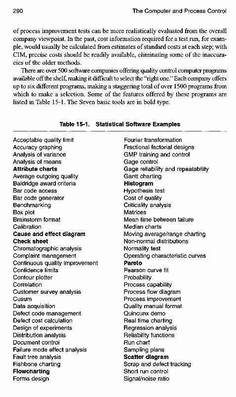
of process improvement tests can be more realistically evaluated from the overallcompany viewpoint. In the past, cost information required for a test run, for exam-ple, would usually be calculated from estimates of standard costs at each step; withCIM, precise costs should be readily available, eliminating some of the inaccura-cies of the older methods.
There are over 500 software companies offering quality control computer programsavailable off the shelf, making it difficult to select the "right one." Each company offersup to six different programs, making a staggering total of over 1500 programs fromwhich to make a selection. Some of the features offered by these programs arelisted in Table 15-1. The Seven basic tools are in bold type.
Table 15-1. Statistical Software Examples
Acceptable quality limitAccuracy graphingAnalysis of varianceAnalysis of meansAttribute chartsAverage outgoing qualityBaldridge award criteriaBar code accessBar code generatorBenchmarkingBox plotBrainstorm formatCalibrationCause and effect diagramCheck sheetChromatographic analysisComplaint managementContinuous quality improvementConfidence limitsContour plotterCorrelationCustomer survey analysisCusumData acquisitionDefect code managementDefect cost calculationDesign of experimentsDistribution analysisDocument controlFailure mode effect analysisFault tree analysisFishbone chartingFlowchartingForms design
Fourier transformationFractional factorial designsGMP training and controlGage controlGage reliability and repeatabilityGantt chartingHistogramHypothesis testCost of qualityCriticality analysisMatricesMean time between failureMedian chartsMoving average/range chartingNon-normal distributionsNormality testOperating characteristic curvesParetoPearson curve fitProbabilityProcess capabilityProcess flow diagramProcess improvementQuality manual formatQuincunx demoReal time chartingRegression analysisReliability functionsRun chartSampling plansScatter diagramScrap and defect trackingShort run controlSignal/noise ratio

It is suggested that quality departments planning to obtain their first programshould give consideration to those which contain the seven basic quality controltools referred to previously. The finer points available in advanced programs canbe obtained later, after the basic procedures have been established. There is littleneed at the outset to have the ability to run Analysis of Variance, or to have Mestof Means available on disk. There is also the danger of blindly selecting a fragmentof a program which looks interesting, draws complicated graphs, and expressesresults of calculations in complex Greek letters, but is an incorrect applicationfor the purpose intended. In one unfortunate instance, an inexperienced qualitymanager selected a process capability graphing routine from the menu of a newprogram, since it "looked good." He then incorrectly used it as a process controlchart for package fill volume control, causing excessive fluctuations of this meas-urement in finished product, with accompanying increased production costs.
ARTIFICIAL INTELLIGENCE AND EXPERT SYSTEMS
Some of the early advances in Expert Systems were made in the food processingindustry. One company, troubled by the advancing age of their most knowledge-able processing engineer, realized that when he retired, he was taking with him alifetime of trouble-shooting techniques that had proven invaluable over the years.They teamed him with a computer expert, with the goal of transferring his expertproduction experience to some type of artificially intelligent computer program.After nearly a year of full-time concentration on this project, a series of disks wasprepared by which operators could readily find expert assistance at solving pro-duction problems with the touch of a computer keyboard. The mind of the expertengineer had been transferred to the computer for ready access! Additionally, thisinformation was expanded with the help of other experts to provide a training pro-gram for new employees. Later another set of expert system disks was preparedfor use by the maintenance department machinists. As more information becameavailable, and as process changes required modifications, this program was read-ily expanded and modified. Since most of the information contained in this typeof program is proprietary, few detailed procedures for this technique are availablein the literature.
Ingredient trackingISO 9000 criteriaSimulationSpectrographic analysisStandard deviationStatistical methodsStatistical process controlStratification analysisSupplier quality assurance
f-Test of meansTaguchi analysisThermal analysisThree-dimension plotterTraceabilityTrainingTrend analysisVariables chartsWeibull curve

There is a real need for this type of information. Most experts tend to buryseveral steps in their reasoning process deep in their subconscious. After the experthas left the company, these reasoning steps may be lost forever, unless recorded aspart of an expert system program. A simple example: once the expert has learnedthat "left makes loose, right makes tight," he no longer needs to go through thisthinking process when he instructs an operator to "turn the controller knob coun-terclockwise." In addition, the expert is not available for consultation on each shiftevery day the plant is operating. Sometimes there are situations where two or threeexperts may be required to offer a solution, and one or more of them might be ona business trip, ill, or on vacation. In their absence, this function is handled inmany organizations by the use of operating manuals; but the need to thumbthrough pages of the "trouble-shooting" section to locate the problem descriptionand its cure often takes much too long to be of practical use.
With expert systems available, productivity can be expected to increase by hav-ing the latest expertise available at each worker's command, avoiding the necessityto shut down a process while seeking an expert. In addition, by having the bestadvice on-line, improvement in decisions affecting quality control are achievable.
Following is a simplified example of how a production operator is able to callup an "expert" in seconds to solve a processing problem. Assume that the processrequires a precise temperature range for control of the product quality, and theoperator observes that the temperature has fallen below the lower limit. He slipshis Expert System disk into his workstation computer and observes a message onthe screen (Figure 15-1).
By checking "Temperature", the next window immediately appears(Figure 15-2).
Checking "Too Low" brings up the next window (Figure 15-3).This window explains the procedure to raise the temperature. In the event that
the instructions do not produce the desired result, checking the "no" square willbring up additional instructions provided by the expert. If the instructions correct
PROCESS: COOKER, POTATO STARCH #6543
Select Problem
Temperature
Pressure
Flow
Color
Figure 15-1. Problem selection.
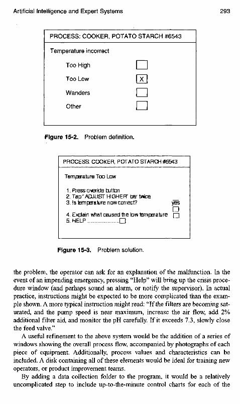
Figure 15-3. Problem solution.
the problem, the operator can ask for an explanation of the malfunction. In theevent of an impending emergency, pressing "Help" will bring up the crisis proce-dure window (and perhaps sound an alarm, or notify the supervisor). In actualpractice, instructions might be expected to be more complicated than the exam-ple shown. A more typical instruction might read: "If the filters are becoming sat-urated, and the pump speed is near maximum, increase the air flow, add 2%additional filter aid, and monitor the pH carefully. If it exceeds 7.3, slowly closethe feed valve."
A useful refinement to the above system would be the addition of a series ofwindows showing the overall process flow, accompanied by photographs of eachpiece of equipment. Additionally, process values and characteristics can beincluded. A disk containing all of these elements would be ideal for training newoperators, or product improvement teams.
By adding a data collection folder to the program, it would be a relativelyuncomplicated step to include up-to-the-minute control charts for each of the
Figure 15-2. Problem definition.
Tern per aiu re Too LJDW
1. Press ovBride button2. Tap" ADUUST HIGHER' bar Mm3. is temperature now correct?
4. Explain what caused tie low temperature5. HELP
yes
PROCESS: COOKER, POTATO STARCH
Temperature incorrect
Too High
Too Low
Wanders
Other
PROCESS: COOKER, POTATO STARCH #6543

parameters (temperature, pressure, flow, color) for quality control and processimprovement studies. Periodic printed control charts could be made available tothe production supervisor and the quality control department.
COMPUTER-CONTROLLED PROCESSING
Before exploring the function of computers in quality control, a review of theprinciples of control might clarify this fairly complex subject. The three stepsinvolved in quality control are measurement, evaluation, and response.
1. The measurement can be made manually, visually or by electrical, mechan-ical, biological, or chemical methods, or by combinations of these.
2. The evaluation compares the measurement to a setpoint (the optimumvalue), and generates an error signal. In statistical quality control terms, thissignal may be expressed as "within 3-sigma, take no action," or "beyond the3-sigma control limits, take action." This class of evaluations may be accom-plished manually or automatically. Another type of evaluation, usually con-ducted by automatic instruments, provides for one of three modes:• Proportional mode control. Measures the magnitude of the error rela-
tive to an acceptable range.• Integral or reset mode control. Measures the magnitude of the error and
relates it to the interval of time over which the error occurred.• Derivative or rate mode of control. Measures the rate at which the error
is changing.3. The response (or feedback signal) is generated by automatic instruments
to reduce the error signal to zero. Older pneumatic and electronic con-trollers are classed as analog devices. Advances in digital computer tech-nology have provided improved methods for control by the use ofcomputer programs to evaluate the error. Commonly, the same modes ofcontrol are utilized: proportional, reset and rate.
A word of caution: unless the statistical principles of process variation are con-sidered when installing instrumented process control, overcontrol might be pro-grammed into a computer system. This may produce a progression of franticsearching by the computer to reduce error in a process which may be perfectly sat-isfactory if left alone. In the worst case, this can produce defects both above andbelow the control limits. A few "sea-going" examples should illustrate overcontrol.
To steer a canoe on a straight course, a correction is made with every stroke ofthe paddle. Occasionally, in a stiff breeze, an extra correction stroke mightbe required. Beyond this, an attempt to correct the oscillation of the canoein mid-stroke would be overcontrol.
Once the course has been set and the rudder has been adjusted, a 100,000 tontanker will continue in a straight line, requiring no correction for hours ata time.

A 10,000 ton freighter in a following sea (waves rolling in approximately thesame direction of travel as the ship), will alternately swing slowly to theleft and then to the right of the course if no rudder adjustment is made.Under this condition however, the overall direction of travel will be in arelatively straight line. If an attempt is made to correct the freighter'sswing by steering in the opposite direction, the freighter will continue itsswing for a few more minutes, and then will respond to both the rudderand the waves to overcorrect in the other direction. The net effect is tocause extremely wide oscillations, each larger than the preceding one. Theoverall direction of travel would be unpredictable.
Once a system is capable of operating successfully within satisfactory limits,using manual control or analog instrumentation, the next step many companiesconsider is the installation of computerized quality control. The ultimate goal isto reduce or eliminate the need for operator intervention. Continuous measure-ments of a process or product may result in large volumes of data which providea guide to controlling quality. There are circumstances—perhaps a small company,or a short production run—where facilities and personnel may not be available toevaluate this data statistically. Here, too, the use of computer technology maysimplify the control of quality.
Selection of the hardware and software to build a satisfactory control systemcan be accomplished in many ways. Perhaps the simplest method is to employ theservices of a consultant who has successfully built effective computerized qualitycontrol systems for other companies in the food industry. Technical and pro-duction personnel should participate in the development and receive training inthe program as it is created. If personnel in quality control and engineering areavailable, the company may elect to provide them with the specialized training tochoose their own program from the hundreds available. The advantage of havingan expert or two on the payroll is obvious; conversely, the disadvantage is the pos-sible promotion or loss of these employees. The use of a team to assist the tech-nical personnel may slow the process somewhat, but should provide thecooperation necessary to make any new system workable.
To construct a new or improved computer-controlled process, a number oflengthy observations and calculations must be prepared. Each stage of the processhas both inputs and outputs from and to many associated process stages. Thesemust be measured and arranged in tabular (or graphical) form so that the opti-mum level of each output can be calculated. Where there are many interrelatedoperations to the overall process, this exploratory step can be very lengthy. Thenext procedure used by many programmers is to connect a series of control instru-ments which simulate the process steps above, and which can be operated atvarious settings to validate the calculations.
For years, these two initial steps had to be performed manually, and usually atgreat expense. Software tools are now available to perform the analysis and sim-ulations more quickly. These programs can then be combined to demonstrate howthe operation would eventually be computer controlled, and how realistically the

theoretical calculations were prepared. By running a series of simulations, theseprograms can accurately forecast the expected output of the process under a num-ber of varying inputs.
Installing a computerized system of production or quality control requiresmajor decisions in three areas:
• What hardware will do the job?• What software will make it work?• How do we prepare the workforce?
Successful installations are rarely those which attempt to cover every aspect ofthe company's operations with a single blanket. Once top management is con-vinced that computer control is the way to go, it is essential that a managementteam be created with the understanding that they will start small, growing asthe payback is demonstrated. The team must also be prepared to solve many newproduction and quality problems, because the ease and speed of computerized datacollection will most surely disclose several problems not previously recognized.Unless these are handled as they occur, the new system will probably fail. If prob-lems are not solved promptly, the same "red lights" will continue to flash everyday, and the effectiveness of the computer will be lost.
Some of the obvious advantages to computer-guided operations are their assis-tance in eliminating operator variability, avoiding use of the wrong or obsoletematerials, instructing operators on performance of their jobs, and entering datadirectly from the measuring device output (calipers, pH meters, thermometers,balances, HPLC). For some applications, data can be color-coded as it is enteredin order to inform the operator if the process is satisfactory (green), marginal(yellow), or in trouble (red). For simplicity, the data can be entered on a speedo-meter dial, a thermometer scale, or stair-step diagram to assist in interpretingthe measurement before the numbers are entered into the statistical data bank forfurther processing and recording. For additional value, the data calculations maybe shown on the computer screen as control charts in real-time to assist the oper-ator, the supervisor, and the manager in evaluating the process while it is under-way. Additionally, the program can continuously produce an updated histogramfor daily, monthly or other comparisons. Of equal importance, a Pareto analysis ofthe problems encountered in the process can be simultaneously constructed andupdated. This would permit anyone interested in the process to determine the mostcritical problems, at any time. Inventory control may continue to be a function ofthe warehouse, but the production floor computers may also be programmed tocontrol inventory as production progresses. Where maintenance scheduling is crit-ical, the process computer may also be used to keep track of machine hours, flash-ing a notice when maintenance performance is approaching. Even in the controllaboratory, a dozen different quality tests can be available for display on the com-puter screen simultaneously, along with control or specification limits, so that out-of-limits data can be immediately signalled for a collection of analyses such ascolor, moisture, pH, flow, solubility, texture, alkalinity, etc. If desired, all of the

information from warehouse, production floor, quality control laboratory, ship-ping and accounting can be "piped" to the CEO's office for real-time evaluationof each department as well as the entire operation. Finally, each analytical toolperformed by the computer may be programmed to flash a warning light or screenmessage when an undesirable condition occurs.
Data Input
In addition to the necessity of providing guidance in operating a process, there aremany other reasons for taking data describing a product's quality characteristics.Some of the common ones:
1. A customer may require data as part of the purchase order. The require-ment may be contractual to certify a lot's conformance to specifications,or it may be considered important to the customer's manufacturing ormarketing systems. The data may or may not have any realistic value tothe customer.
2. The CEO or the legal department may wish to have ample files asbackup in the event of a product quality failure, resulting in a recall or alawsuit.
3. A databank of purchased raw material performance may be a useful toolin negotiating price.
4. A confused or untrained management might ask for volumes of assorteddata with the hope of finding a clue to areas for quality improvement.
5. Defect data might be accumulated by incoming shipments to assist inselection of a supplier.
6. A large file on competitive product quality might be a useful tool forbenchmarking purposes.
It is likely that there are another half-dozen reasons for collecting data, butthere are four general levels of information which seem to be commonly requiredby all companies:
1. Top management wants information on an 8| X 11 piece of paper which
tells them "what's going on," an overview of what is happening.2. On the shop floor, the workers need the type of information which will
give them data regarding the variability of the process, allowing them totake action in real time.
3. Middle management (QC or Engineering) uses parcels of information tostatistically analyze and compare—after the fact. They may be interestedin comparing shifts, machines, products, processes, production days,operators, material supplier performance.

4. Product and process improvement teams or Research and Developmentusually require large masses of past data in their efforts to reach theirgoals.
Middle management needs considerable more information than is required forimmediate use by workers on the production floor. The data may have to betagged with shift, machine, product, serial number, lot size, etc. labels for furtheranalysis.
The major advantages of electronic data collection and transmission are accu-racy and speed. Collecting data by individual hand measurement, writing the dataonto a form, calculating or summarizing, and copying it onto a chart presentsopportunities for making an error (is that figure a 7 or a 5?), and requires far moretime to perform than does an electronic system. It has been found in a detailedstudy that mistakes in writing down and reading numbers can run as high as 12%of the time. A major improvement over copying data by hand would be to enter theinformation through a computer keyboard, although the opportunity for errors stillexists. Variable data can be collected from virtually any electronic output—gages,calipers, pH meters, chromatographs, scales, etc.—and be transmitted error-freethrough one of many relatively inexpensive "black boxes" to computers for display,storage, or further processing.
One effective method of collecting attribute data is the use of a bar code.Hand-held devices are available which can be programmed to read bar codes,store, calculate, or transmit the information to a master computer. They can beprogrammed to perform specific tasks, or they can be purchased pre-programmedfor general use. In addition to the obvious functions of a bar code for identifyingraw materials on the receiving dock and finished product in the warehouse, theyare also used to classify blocks of data collected at specific stages on the produc-tion line.
Before investing in an electronic data collection system, one must be sure thatthere is no proprietary function in the black box which will make it impossible touse for a particular operation. There is a myriad of products available, but someof them are programmed to handle a specific function which might not be appli-cable to the process under consideration.
Some hand-held computers, such as personal organizer units, are availablewhich can be programmed to contain the day's schedule, which accept pen inputfor notes or graphics, and which can be down-loaded to desktop computers forfurther processing or recording.
Modules are available which can accept voice data—in any language. Otherscan speak to the operator in phrases or whole pages which are highlighted onthe screen. This capability is of value where the employees are not proficient inreading, or need translation.
Through the use of video cameras and video recorders, tapes of a process canbe readily prepared while in operation, to be used as a training film for otheremployees at the same or different locations. If required, instantaneous transferof such tapes can be made using a modem and telephone lines, thus permitting

interchange of ideas between widely separated plants while operating or modify-ing a process.
Sensing Devices
A sensor is a device which reacts to a physical or chemical stimulus to produce acorresponding electrical signal proportional to the physical parameters measured.As generally understood, a sensor is another word for a transducer. In the exampleabove for an Expert System, four such sensors were used to control a process forcooking potato starch: temperature detector, pressure measuring device, flow rateinstrument and color analyzer. Each of these sensors responded to specific stim-uli, and converted the relative response to an electrical signal which in turn wassent ultimately to the computer at the workstation. The signal was then processedby a computer program and returned to an operating device (such as a solenoidvalve) which would appropriately adjust the physical condition as required tomaintain control. In the event of a physical condition beyond the control limits forwhich the program was defined, an out-of-limits notice was issued on screen forthe operator's attention (the temperature, in the example shown). As an additionaltool for the operator, an overall pictorial of the process under his control may beincluded in the program as shown in Figure 15-4. It shows the major equipment,and the relative location of the sensors and controllers.
Sensors are available for countless conditions and respond to stimuli using awide variety of principles. Temperature sensors, for example, may be classifiedas thermocouples (TC), resistance temperature detectors (RTD), thermistors, andIC sensors.
Other sensors are listed in Table 15-2.
Figure 15-4. Process flow controls.
Flow
Color
Pressure
Temperature
SolenoidValve
Pressure PumpHeaterFlowColor Additive

Table 15-2. Sensors
Sensors
Infra-red, conductivityPolymer resinsBioreactorTurbidimetersColorimeterInfra-redElectrical resistanceX-rayGamma ray, scalesGamma raysReflectometerInfra-redGamma rayStrain gageDifferential pressurePolarized or IR lightStrain gage/BrinellVisible lightFloat, strain gagePhotocellProximity switchStrain gageInfra-redpH cellPressure transducerPhotocellMicrophoneViscometerRefractometerInfra-redInfra-redThermocoupleConductivityRheometer
Measurement
AcidAromaBOD (high speed)ClarityColorComposition (chemical)ConcentrationContamination, solidCountDensityDefect (visual)FatFill levelForceLow rateGlass chipsHardnessLabels (missing, faulty)LevelLightMotionMass (weight)MoisturePHPressureSeal area contaminationSoundShearSolidsSugarSulfur dioxideTemperatureTotal acidViscosity
Note that Flowmeters can be based on differential pressure, magnetic sensor,vortex, coriolis effect, thermal mass, positive displacement, turbine, ultrasonic,and other sensors. Level sensors may also be triggered by capacitance/RF,hydrostatic pressure, float switch, photocell, radar/microwave, ultrasonics, loadcell, conductance instrument, point switches.
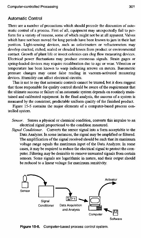
Automatic Control
There are a number of precautions which should precede the discussion of auto-matic control of a process. First of all, equipment may unexpectedly fail to per-form for a variety of reasons, some of which might not be at all apparent. Valveswhich have not been moved for long periods have been known to jam in their lastposition. Light-sensing devices, such as colorimeters or refractometers maydevelop cracked, etched, scaled or clouded lenses from product or environmentalcontact. Growth of plant life or insect colonies can clog flow measuring devices.Electrical power fluctuations may produce erroneous signals. Strain gages orspring-loaded devices may require recalibration due to age or wear. Vibration ortemperature has been known to warp indicating arrows on meters. Barometricpressure changes may cause false reading in vacuum-activated measuringdevices. Humidity can affect electrical circuits.
This is not to say that automatic controls cannot be trusted, but it does suggestthat those responsible for quality control should be aware of the requirement thatthe ultimate success or failure of an automatic system depends on routinely main-tained and calibrated equipment. In the final analysis, the success of a system ismeasured by the consistent, predictable uniform quality of the finished product.
Figure 15-5 contains the major elements of a computer-based process con-trolled system.
Sensor. Senses a physical or chemical condition, converts this impulse to anelectrical signal proportional to the condition measured.
Signal Conditioner. Converts the sensor signal into a form acceptable to theData Analyzer. In some instances, the signal may be amplified or filtered.The amplification of the signal received should be such that its maximumvoltage range equals the maximum input of the Data Analyzer. In somecases, it may be required to reduce the electrical signal to protect the com-puter. Filtering may be desirable to remove unwanted signals from certainsensors. Some signals are logarithmic in nature, and their output shouldbe reduced to a linear voltage for maximum sensitivity.
Activator
Software
Computer
Data Acquisitionand Analysis
SignalConditioner
Sensor
Figure 15-5. Computer-based process control system.

Data Acquisition Board (DAB). Accepts signals from a number of channels,at specified sampling rates and types of inputs. The sampling rates areoften determined by the ability of a DAB to multiplex, that is, switch fromchannel to channel. These boards are available in a wide array of capabil-ities and outputs.
Computer. Most computers have sufficient computational power to handlethe output of available DABs. If necessary, however, special analysishardware is available. Calculations can be performed in the millions persecond, allowing a computer to handle many inputs from the DAB atextremely high speed.
Software. Some companies might prefer to develop their own software toprogram the hardware. It is probably quicker (and certainly simpler) topurchase driver software from the manufacturer of the DAB. The use ofapplication software will add presentation and analysis capabilities to thedriver software.
Activator. Outputs from the computer in automatic control systems are pri-marily concerned with operating control devices such as valves, motordrives, positioning arms, mixers, fans and other powered equipment.Expert System inputs/outputs can also be programmed into some systems.As discussed above, the computer quality control calculating output cantake the form of data compilations, control charts, run charts, and manyother graphs.
As mentioned above, the computer makes data analysis both easy and rapid. Inaddition to the control charts which can be instantly calculated and viewed by theline operator, the same data can be downloaded or connected through computernetworks to quality control and process engineers for further analysis.
Consider the following simplified example. A small company manufacturesa family of drink mixes, using a simple system as shown in the flow chart(Figure 15-6).
The raw ingredients are weighed manually, and dumped into a screw blendorwhich discharges through a feed bin into a four-scale filler head. The products arepackaged in composite foil cannisters, and cased after labeling. Net weights arechecked occasionally. The major reason for checkweighing is to reduce productgiveaway and to avoid the possibility creating seam cutovers from over filling.
The principle customer has specified that the net weights should average 454 g,with an acceptable range of 445-^63 g. Over the years, this customer has com-plained about underweights on several occasions, and has returned the offendingshipments for reworking—that is, hand sorting and removing the underweightcontainers. Eventually, this customer tired of the delays resulting from the weightproblem and threatened to take his business elsewhere. The customer sug-gested contacting the Smathers Scale Company, which manufactured automaticcheckweighers.
The Smathers representative brought in an automatic checkweigher and datacomputer for a demonstration. While it was being assembled and wired into the

Figure 15-6. Drink mix flow chart.
line, the representative took 50 consecutive samples of orange drink mix off theline as produced. Over the next several hours he weighed each can, subtractingthe tare weight, then calculated the process capability based on these samples,using a hand-held calculator.
The calculations showed that over an extended run, the process would beexpected to produce nearly 10% below the lower specification limit of 445 g, andabout 6% above the upper specification limit of 463 g. This came as a shock tothe owner, who had assumed that the four filler scales were always reliable.
The following day, the automatic Smathers equipment was ready to demon-strate. The checkweigher system gross weighed each cannister as it passed over astrain gage, adjusting for the tare. The electrical signal generated was picked upby a computer, which stored the data, and was programmed to perform a numberof statistical functions. The line speed was running at the usual 45 cannisters perminute, and in less than two minutes, nearly 100 weighings were recorded in thecomputer. Smathers then pressed the PROCESS CAPABILITY button on theconsole, and selected the CALCULATE option. A number of statistical calcula-tions appeared on the computer screen within seconds:
Sample size 50Mean 453.206Standard deviation 6.32257Three-Sigma limits 434.238-472.174
Weigh
ColorSugarDextroseAcidFlavor
Blendor
4 head scale
Sealer Labeler Caser To warehouse
Filled cannisters

Lower specification limit 445Upper specification limit 463CPK 0.43263CP Index 0.474491% Under LSL of 445 9.7%% Over USL of 463 6.1%
To further demonstrate the effectiveness of the system, Smathers then selectedthe GRAPH option, and the following graph appeared on the computer screenwithin a few seconds. The data, calculations and graph all showed that the systemwas not capable of satisfying the customer's requirements.
The graph (Figure 15-7) and calculations convinced the owner that the scaleswere in need of maintenance. The counterweights were adjusted to the precisedelivery weights, and the knife edge scale bearings were honed. With the assis-tance of the Smathers representative, another fifty samples were automaticallyweighed and recorded in the computer. The resulting chart (Figure 15-8) showedthat the line was now capable of producing at least the minimum weight, althoughsome overweights could still be expected. Changing the line speed would probablypermit some control over the average weight value, but the process was marginal.
After much discussion, it was decided that better density control could narrowthe weight range, and combined with the improved line maintenance, perhapsgood control might be attained. The density could be adjusted by varying theblendor time for each batch (Figure 15-9). Once the ideal blendor duration wasestablished, another set of data was fed into the computer and analyzed with thefollowing results:
RE
LAT
IVE
FR
EQ
UE
NC
Y
net weight
Figure 15-7. Initial capability analysis.

RE
LAT
IVE
FR
EQ
UE
NC
Y
Mean
Net Weight, grams
Figure 15-8. Capability analysis after maintenance.
RE
LAT
IVE
FR
EQ
UE
NC
Y
Net Weight, grams
Figure 15-9. Capability analysis with density control.
The PROCESS CAPABILITY-CALCULATE buttons were activated, producingthe following data:
Sample size 50Mean 453.624Standard deviation 2.65196Three-Sigma limits 445.668-461.58
Mean USL

Lower specification limit 445Upper specification limit 463CPK 1.08398CP Index 1.13124% Under LSL of 445 0.1 %% Over USL of 463 0.0%
To demonstrate the flexibility of the Smathers computer programs (and to fur-ther assist in closing the sale), some of the other features were demonstrated bythe simple pressing of the appropriate computer panel buttons. Using the datafrom the capability study with density control (the final test conditions), the con-trol charts were instantly constructed (Figures 15-10 and 15-11).
Figure 15-10. Net weight control chart (with maintenance, and densitycontrol).
Subgroup Number
Figure 15-11. Net weight range control chart.
Subgroup Number
Gra
ms
Gra
ms

By depressing the DATA button, the fifty data points used to construct the pre-ceding control charts were printed out in seconds. Two other charts were alsodemonstrated: trend analysis and X/Y chart.
This simple example has demonstrated the speed with which computers cansolve production problems, calculate and graph results of changes, and providehigh speed calculations in process improvement studies.
SUMMARY
To summarize, a computer system can be installed on the factory floor to permitthe operator to enter and observe data with reference to standards. The data maybe combined with previous information to produce control charts for review bythe operator, the supervisor, or the manager to evaluate the process at any timewith respect to current or prior performance. The computer might serve as anexpert with push-button information to guide the operator in performance of hiswork. Various signals or alarms may be included to notify the operator of the needfor remedial action. The signals received by the computer may bypass the opera-tor and automatically trigger control reactions to operate the process at optimumconditions. Finally, the data may be stored or transferred to other computer banksfor further analysis or for historical purposes.

16 Six-Sigma
The six-sigma program for quality improvement and control outlined in Chapter 1has provided many hardware companies with a method of greatly increasing prof-its by reducing costs associated with every department in the company, and byproduct reliability improvements. The program requires that every employee beaccountable for understanding and implementing six-sigma. This conflicts withDr. Deming's principle that 85% of the quality problems are faults of the systemwhich can be corrected only by management.
"Quality" has been defined by Dr. Mikel Harry as a "state in which valueentitlement is realized for the customer and provider in every aspect of the busi-ness relationship. When a process reaches six-sigma control, only 3.4 defects permillion will be produced."
The major concerns with process improvement under this system are reworkand repair costs. This has little relation to quality controls in the food industry. Forexample, one of the major steps in implementation of six-sigma is to arbitrarilyincrease the central tendency (average) quality value of a process by 1.5-sigma,since this is considered to be related to machine wear during processing. Again,this has little application in the food industry. In fact, for packaged food net weightquality control, arbitrarily moving the central tendency higher by 1.5-sigma couldbe a financial disaster.
The control limits of a hardware process using the six-sigma system are deter-mined by counting the defects produced by a process and comparing this figurewith a table. When the process average is shifted by 1.5-sigma, the "Defects perMillion Opportunities" is shown below.
Percent non-defective Defects per million Sigma
93.3 66,807 399.4 6,210 499.97 233 599.999 3.4 6

Several major hardware and electronic equipment companies have adoptedthis system and are enthusiastic about the reduction of complaints and the savingsachieved.
Unlike three-sigma statistical quality control procedures, the upper specifica-tion limit for a six-sigma system is at six-sigma, and the lower specification limitis set at zero. In the three-sigma statistical quality control procedure, the upperand lower specification limits are determined by customer requirements or byindustry standards.
Furthermore, in the three-sigma system, if a product characteristic reaches theupper or lower control limits, the product is resampled immediately; and if stillbeyond the limits, the process is stopped until the problem is corrected. This doesnot suggest that any product has been produced beyond the specification limit.In fact, under the three-sigma system, it is possible that a defect will rarely beproduced. As the process is improved, the three-sigma limits are reset closertogether and further away from the specification limits, thus reducing the possi-bility of ever producing a defect.
It should be emphasized that in the food industry, critical defects which might beinjurious to health are never permitted, whereas in some hardware industries, prod-ucts can be returned under warranty for replacement or repair. As an example ofthis basic principle in the food industry, consider the need for absolute food safetyin a fast-food hamburger restaurant chain.
• 500 hamburgers served each day by 1 restaurant• 2,000,000 served each day by the 4,000 restaurants in the chain• 730 million served by the chain in a year• Assume that the chain can achieve five-sigma defect control• Defect tables, at five-sigma, predict 233 defects per million• If 233 hamburgers contained salmonella at five-sigma control, then 170,000
customers would become violently ill in a year.
Obviously this cannot be permitted. There was a case where a tainted shipmentarrived at a fast-food restaurant, and several customers became ill. Worse still,one small child actually died. This event was so rare in the food industry, the storywas on radio stations and in newspapers across the country. The companypromptly initiated preventive measures, but came very close to becoming a failedbusiness. Unsafe food products cannot leave the plant.
If, in spite of the cautions noted above, management of a food processing com-pany insists on investigating a six-sigma system, following is a digest of the stepsgenerally agreed upon by six-sigma enthusiasts.
Step 1. Recognize
At the outset, the executive leading the process must understand that the majorgoal is determined not by the reduction of defects or improvement of profits, butrather it is meeting the requirements and satisfaction of the consumer. Defect

reduction and profit improvement are by-products of this concept. This steprequires studies to identify procedures which affect principle business systems,and how they affect customers. In the language of six-sigma, these systems areknown as "processes." The areas investigated are identification of the core values,precise definition of products supplied to customers, and the interrelationships ofall of the company's processes.
Identification of the company's processes is a vital beginning, but at the same time,"benchmarking" competitors' processes is obviously of value at the Recognize stage.Exploring noncompeting companies is suggested where possible, since they frequentlyhave processes which can be adapted. These processes may not necessarily be propri-etary, nor even directly applicable. However they assist in determining some of theprocesses to explore and improve. In addition to assisting in identification of themost important processes, benchmarking can frequently prioritize improvementcandidates.
Step 2. Define
The "Recognize" step may produce a large number of possibilities for improve-ment. The task during the "Define" stage is to select the three or four processeswhich are most likely to improve customer satisfaction. Emphasis should beplaced on information gathered during customer surveys. From this information,establish standards and define which areas of the company require further study.This procedure should result in defining standards from the customer's point ofview. Establish critical features of products required by the customer. Concludehow the company and the customer should interact. Expertise of managementpersonnel who had originally prepared specifications based on their own experi-ence may recognize that these standards require tailoring to customer needs.
Critical outputs from the processes selected are identified since they willsubsequently be used to evaluate capability. In addition to defining key processes,it is also wise to identify key customers and determine the differing relationshipsof the processes selected. There are other considerations which may identify themost important processes: use of raw materials, potential cost savings, estimatedtime to solve, manpower requirements, effect on other processes, etc.
Step 3. Measure
Based on the results of the customer survey, conduct statistical studies of thoseareas of the company which have a direct bearing on the customer satisfactionneeds identified in Step 2. Determine from these studies those areas whichrequire further attention. In addition to product and customer emphasis, thesestudies may provide the basis for improving process costs. An efficient systemshould be established to closely control critical customer requirements duringprocessing. The sigma ratings for each process should be studied to determinewhich candidates are most critical. At this stage, statistical process control tech-niques should be evaluated: process capability, product failure analysis, control

limits versus specifications. By introducing vigorous statistical techniques,changes in the process (both favorable and unfavorable) can be recognized forappropriate action.
Step 4. Analyze
Prioritize the critical studies of Step 3, based on their standard deviations. Thosewith the lowest sigma will require the most improvement. Examples of criticalstudies are customer complaints, defective materials, marginal product perform-ance, slow response time to complaints, price of the product, poor design whencompared to competitors. Identify those processes which affect consumerrequirements, and those which affect process costs and variability. Compare theproject conclusions with organization goals.
Step 5. Improve
By the use of teams headed by a six-sigma specialist, explore methods by which thelow sigma operations can be improved. It is interesting to compare this part of thesix-sigma process with the Deming concept of improvement. The six-sigma conceptas practiced by some hardware industries includes line operators. Managementrecognizes that line operators know more about the details of their part of themanufacturing process than the heads of sales department, the engineers, theaccountants, or the shipping department managers. Dr. Deming has stated thatteams which include line operators may be disappointed with their abilities tosuggest valid improvements to the operation. Line operators are probably unfa-miliar with the technical requirements (biological, structural, legal, financial orsafety) of their department when compared to other employees who are trainedfor these specialized responsibilities. There is also the probability that line oper-ators may not have the same interest, education or drive necessary for successfulteam studies. There are other considerations. Many employees are content to twistthe knobs, turn on the switches, and pick up their paycheck; some may fear thatany change in the procedure might be more difficult, or might possibly lead to anend to their employment. In all other respects, the Deming approach emphasizesthe use of management teams.
Step 6. Control
Once the data confirms that the improvement goal of the project has beenreached, written procedures are prepared to provide employees with the specificinstructions that will produce the desired product or process. Procedures to ensurethat the steps are followed and that the expected improvements are realized shouldbe documented. During early operations of the new process, a leader should beassigned by management to ensure that the proper steps are being followed andthat the desired results are achieved. Progress reports are to be prepared by theleader to include suggestions for solving problems which might occur. It is also

suggested that at this stage, a report might be issued to explain the new process,giving credit to the team members who were instrumental in preparing the newprocess.
Step 7. Standardize
One organization has organized this step into three phases: at the business level,at the operational level, and at the process level. If a particular process has gonethrough all of these steps and has proved successful, consideration should begiven to applying the same principles to other processes in the company. Thereare companies where upper management prefers to operate based on experienceand intuition. When six-sigma-designed process improvements are successful,and when the standardized success in one area can be applied to others, thesemanagers are more likely to appreciate and utilize the six-sigma process.
Step 8. Integrate
Having successfully passed through all of the above steps, one of the most diffi-cult steps is the integration of the new philosophy into the company policy. Thisis partially because of inherent resistance to change. Many companies find thatthey can sometimes solve process problems through simple reasoning instead ofthe complex six-sigma technique. In some instances, rewards such as extra com-pensation for six-sigma accomplishments may convince management (and lowerlevel employees as well) that this technique is worth supporting.
By standardizing the process of problem solving and integrating this processinto company policy, future problems may be explored more efficiently usingexisting techniques.
SUMMARY
The six-sigma process of quality control and problem solving is a carefullyconstructed and relatively complicated procedure which has been successfullyused by several hardware manufacturers. It is a complicated extension of theDeming technique: Plan/Do/Check/Act (see Chapter 14). Food processors mayfind the technique useful, with the single exception of determining the sigmacharacter of their processes by counting defects and setting the goal of six-sigmaat the process control limits. The dangers of this technique have been explainedpreviously.

^^c' or np
0.020.040.060.080.10
0.150.200.250.30
0.350.400.450.50
0.550.600.650.700.75
0.800.850.900.951.00
O
X
980961942923905
861819779741
705670638607
577549522497472
449427407387368
1
1,000999998997995
990982974963
951938925910
894878861844827
809791772754736
2
1,0001,0001,0001,000
999999998996994992989986
982977972966959
953945937929920
3
1,0001,0001,0001,000
1,000999999998
998997996994993
991989987984981
4
1,0001,0001,000
1,0001,000999999999
999998998997996
5
1,0001,0001,000
1,0001,0001,0001,000999
6
1,000
7 8 9
Table A-1. Summation of Terms of the Poisson Exponential BinomialDistribution Limit
Entries in the table, when multiplied by 10~3, represent the probabilities of cor fewerdefects, defectives, or occurrences when the expected or average number is np'.
Appendix

Table A-1 . (continued)
\cc'or npN
1.11.21.31.41.51.61.71.81.92.02.22.42.62.83.0
3.23.43.63.84.0
4.24.44.64.85.0
5.25.45.65.86.0
2.83.03.23.43.63.84.04.24.4
O
\
333301273247223202183165150135111091074061050
041033027022018015012010008007
006005004003002
10
1,0001,0001,000999999998997
996994
1
699663627592558
525493463434406
355308267231199
171147126107092
078066056048040
034029024021017
11
1,0001,000999999
999998
2
900879857833809
783757731704677
623570518469423
380340303269238
210185163143125
109095082072062
12
1,0001,000
1,000999
3
974966957946934
921907891875857
819779736692647
603558515473433
395359326294265
238213191170151
13
1,000
4
995992989986981976970964956947
928904877848815
781744706668629
590551513476440
406373342313285
14
5
999998998997996994992990987983
975964951935916
895871844816785
753720686651616
581546512478446
15
6
1,0001,0001,000999999
999998997997995
993988983976966
955942927909889
867844818791762
732702670638606
16
7
1,0001,000
1,0001,000999999999
998997995992988
983977969960949
936921905887867
845822797771744
8
1,0001,0001,000
1,000999999998996
994992988984979
972964955944932
918903886867847
9
1,0001,000999999
998997996994992
989985980975968
960951941929916

Table A-1 . (continued)
\sC
c'or np
4.64.85.05.25.45.65.86.0
6.26.46.66.87.07.27.47.67.8
8.08.59.09.5
10.0
6.26.46.66.87.07.27.47.67.8
8.08.59.09.5
10.0
10
\
992990986
982977972965957
O
002002001001001
001001001000
000000000000000
10
949939927915901887871854835
816763706645583
11
997996995
993990988984980
1
015012010009007
006005004004
003002001001000
11
975969963955947
937926915902
888849803752697
12
999999998
997996995993991
2
054046040034030
025022019016
014009006004003
12
989986982978973967961954945
936909876836792
13
1,0001,000999
999999998997996
3
134119105093082072063055048
042030021015010
13
995994992990987
984980976971
966949926898864
14
1,000
1,0001,000999999999
4
259235213192173
156140125112
100074055040029
14
998997997996994
993991989986
983973959940917
15
1,0001,000999
5
414384355327301
276253231210
191150116089067
15
999999999998998997996995993
992986978967951
16
1,000
6
574542511480450
420392365338
313256207165130
16
1,0001,000999999999
999998998997
996993989982973
7
716687658628599
569539510481
453386324269220
17
1,0001,0001,000
999999999999
998997995991986
8
826803780755729
703676648620
593523456392333
18
1,0001,0001,0001,000
999999998996993
9
902886869850830
810788765741
717653587522458
19
1,000999999998997

Table A-1 . (continued)
\xC
c'or np x
8.59.09.5
10.0
c' or np' c
10.511.011.512.012.513.013.514.014.515.0
10.511.011.512.012.513.013.514.014.515.0
10.511.011.512.012.513.013.514.014.515.0
20NV
1,0001,000999998
O
000000000000000000000000000000
10
521460402347297252211176145118
20
997995992988983975965952936917
21
1,000999
1
000000000000000000000000000000
11
639579520462406353304260220185
21
999998996994991986980971960947
22
1,000
2
002001001001000000000000000000
12
742689633576519463409358311268
22
999999998997995992989983976967
3
007005003002002001001000000000
13
825781733682628573518464413363
23
1,0001,000999999998996994991986981
4
021015011008005004003002001001
14
888854815772725675623570518466
24
1,000999999998997995992989
5
050038028020015011008006004003
15
932907878844806764718669619568
25
1,000999999998997996994
6
102079060046035026019014010008
16
960944924899869835798756711664
26
1 ,0001,000999999998997
7
179143114090070054041032024018
17
978968954937916890861827790749
27
1,000999999998
8
279232191155125100079062048037
18
988982974963948930908883853819
28
1,000999999
9
397341289242201166135109088070
19
994991986979969957942923901875
29
1,0001,000

Table A-1 . (continued)
^XCc' or n/rx
16171819202122232425
16171819202122232425
16171819202122232425
1920212223
4
\000000000000000000000000000000
14
368281208150105072048031020012
24
978959932893843782712635554473
34
999990997994988
5
001001000000000000000000000000
15
467371287215157111077052034022
25
987975955927888838777708632553
35
1,000999998996993
6
004002001001000000000000000000
16
566468375292221163117082056038
26
993985972951922883832772704629
36
1,000999998996
7
010005003002001000000000000000
17
659564469378297227169123087060
27
996991983969948917877827768700
37
999999997
8
022013007004002001001000000000
18
742655562469381302232175128092
28
998995990980966944913873823763
38
1,000999999
9
043026015009005003002001000000
19
812736651561470384306238180134
29
999997994988978963940908868818
39
1,000999
10
077049030018011006004002001001
20
868805731647559471387310243185
30
999999997993987976959936904863
40
1,000
11
127085055035021013008004003001
21
911861799725644558472389314247
31
1,000999998996992985973956932900
41
12
193135092061039025015009005003
22
942905855793721640556472392318
32
1,000999998995991983971953929
42
13
275201143098066043028017011006
23
963937899849787716637555473394
33
1,000999997994989981969950
43

Area to the right of z (or to the left of -z), or the probability of a random value ofz exceeding the marginal value.
ZQ
0.00.10.20.30.4
0.50.60.70.80.9
1.01.11.21.31.4
1.51.61.71.81.9
2.02.12.22.32.4
.00
.500
.460
.421
.382
.345
.309
.274
.242
.212
.184
.159
.136
.115
.097
.081
.067
.055
.045
.036
.029
.023
.018
.014
.011
.008
.01
.496
.456
.417
.378
.341
.305
.271
.239
.209
.181
.156
.133
.113
.095
.079
.066
.054
.044
.035
.028
.022
.017
.014
.010
.008
.02
.492
.452
.413
.374
.337
.302
.268
.236
.206
.179
.154
.131
.111
.093
.078
.064
.053
.043
.034
.027
.022
.017
.013
.010
.008
.03
.488
.448
.409
.371
.334
.298
.264
.233
.203
.176
.152
.129
.109
.092
.076
.063
.052
.042
.034
.027
.021
.017
.013
.010
.008
.04
.484
.444
.405
.367
.330
.295
.261
.230
.200
.174
.149
.127
.107
.090
.075
.062
.051
.041
.033
.026
.021
.016
.013
.010
.007
.05
.480
.440
.401
.363
.326
.291
.258
.227
.198
.171
.147
.125
.106
.089
.074
.061
.049
.040
.032
.026
.020
.016
.012
.009
.007
.06
.476
.436
.397
.359
.323
.288
.255
.224
.195
.169
.145
.123
.104
.087
.072
.059
.048
.039
.031
.025
.020
.015
.012
.009
.007
.07
.472
.433
.394
.356
.319
.284
.251
.221
.192
.166
.142
.121
.102
.085
.071
.058
.047
.038
.031
.024
.019
.015
.012
.009
.007
.08
.468
.429
.390
.352
.316
.281
.248
.218
.189
.164
.140
.119
.100
.084
.069
.057
.046
.038
.030
.024
.019
.015
.011
.009
.007
.09
.464
.425
.386
.348
.312
.278
.245
.215
.187
.161
.138
.117
.099
.082
.068
.056
.046
.037
.029
.023
.018
.014
.011
.008
.006
Table A-2. Areas under the Normal Probability Curve
Table A-1. (continued)
^\ C
c' or np^x
2425
34
\
979966
35
987978
36
992985
37
995991
38
997994
39
998997
40
999998
41
999999
42
1,000999
43
1,000
Credit: Eugene L. Grant, Statistical quality control, 3rd ed. (New York: McGraw-Hill BookCompany, 1964).

Table A-2. (continued)
ZQ
2.52.62.72.82.92.3.4.5.
Detail of tall (.2135, for example, means .00135)
.006
.005
.003
.003
.002.i228.21354317.6287
0.0
.006
.005
.003
.002
.002!179.39684207.6170
0.1
.006
.004
.003
.002
.002!139.36874133.7996
0.2
.006
.004
.003
.002
.002!107.34835854.7579
0.3
.006
.004
.003
.002
.0022820.33375541.7333
0.4
.005
.004
.003
.002
.002262132335340.7190
0.5
.005
.004
.003
.002
.002
2466.3159.s211.7107
0.6
.005
.004
.003
.002
.0012347.31085130.8599
0.7
.005
.004
.003
.002
.001.22564723.6793.8332
0.8
.005
.004
.003
.002
.001.21874481.6479.8182
0.9
Credit: Ronald J. Wonnacott and Thomas H. Wonnacott, Introductory statistics, 4th ed.(New York: John Wiley & Sons, 1985).
Table A-3. Values of f
\ a
V \
1234
56789
1011121314
1516171819
202122
Two-tail critical values
0.50\
1 .000000.816500.764890.74070
0.726690.717560.711140.706390.70272
0.699810.697450.695480.693840.69242
0.691200.690130.689190.688370.68763
0.686960.686350.68580
0.25
2.41421 .60361 .42261 .3444
1 .30091.27331 .25431.24031 .2297
1.22131.21451 .20891.20411 .2001
1.19671.19371.19101.18871.1866
1.18481.18311.1816
0.10
6.31382.92002.35342.1318
2.01501.94321 .89461 .85951.8331
1.81251 .79591 .78231.77091.7613
1 .75301 .74591 .73961.73411.7291
1.72471.72071.7171
0.05
12.7064.30273.18252.7764
2.57062.44692.36462.30602.2622
2.22812.20102.17882.16042.1448
2.13152.11992.10982.10092.0930
2.08602.07962.0739
0.025
25.4526.20534.17653.4954
3.16342.96872.84122.75152.6850
2.63382.59312.56002.53262.5096
2.48992.47292.45812.44502.4334
2.42312.41382.4055
0.01
63.6579.92485.84094.6041
4.03213.70743.49953.35543.2498
3.16933.10583.05453.01232.9768
2.94672.92082.89822.87842.8609
2.84532.83142.8188
0.005
127.3214.0897.45335.5976
4.77334.31684.02933.83253.6897
3.58143.49663.42843.37253.3257
3.28603.25203.22253.19663.1737
3.15343.13523.1188

Table A-3. (continued)
\ U Two-tail critical values
V
23242526272829304060120OO
V /
/ a
\ 0.50
0.685310.684850.684430.684050.683700.683350.683040.682760.680660.678620.676560.67449
' 0.25
0.25
1.18021.17891.17771.17661.17571.17481.17391.17311.16731.16161.15591.1503
0.125
0.10
1.71391.71091.70811.70561 .70331 .701 11.69911.69731.68391.67071.65771 .6449
0.05
0.05
2.06872.06392.05952.05552.05182.04842.04522.04232.02112.00031.97991 .9600
0.025
0.025
2.39792.39102.38462.37882.37342.36852.36382.35962.32892.29912.26992.2414
0.0125
0.01
2.80732.79692.78742.77872.77072.76332.75642.75002.70452.66032.61742.5758
0.005
0.005
3.10403.09053.07823.06693.05653.04693.03803.02982.97122.91462.85992.8070
0.0025
One-tail critical values
Credit: E. S. Pearson, Critical values of Student's t distribution. Biometrika 32 (1941):168-181.
Table A-4. Binomial Coefficients
n (8) (?) fn\(2) (3) (4
n) (S) (8) (?) /n\(B) tn\(B) do)
O1234
56
11111
11
1234
56
136
1015
14
1020
1
515
16 1

Table A-4. (continued)
n
789
1011121314
1516171819
20
(S)
11111111111111
(?)789
1011121314
1516171819
20
(S)
212836
4555667891
105120136153171
190
(S)
355684
120165220286364
455560680816969
1140
(2)
3570126
2103304957151001
13651820238030603876
4845
(S)
2156126
25246279212872002
300343686188856811628
15504
(8)
72884
21046292417163003
50058008123761856427132
38760
(?)
1836
12033079217163432
643511440194483182450388
77520
(S)
19
4516549512873003
643512870243104375875582
125970
(S)
1
10552207152002
500511440243104862092378
167960
dno)
111662861001
30038008194484375892378
184756
Table A-5. Random Numbers
102753962328 41 50 61 8834 21 42 57 0261 81 77 23 2361 15181354
91 76 21 64 64OO 97 79 08 06364618349488 98 99 60 5004 37 59 87 21
63 62 06 34 4178 47 23 53 90876862 1543476092107756 88 87 59 41
71 50 54 36 2364852720185919 18974882 82 1 1 54 081686202688
4491 13329737 30 28 59 8575 20 80 27 7765 95 79 42 940502032417
94 21 78 55 0934 41 92 45 71531436592588595311 5265 28 04 67 53
54 31 04 82 9883 36 36 05 5680 30 03 30 9853 28 70 58 9690 74 80 55 09
75 31 62 66 5453 56 68 53 407891 69160093 62 40 89 9647 97 81 56 51
727645 169409 23 70 70 0754473370-1566 25 69 07 0495 79 88 37 31
041412 150939 71 65 09 6205 24 67 70 0744 07 39 55 4314539051 17
84 80 32 75 7701 74 39 59 73084318736843 56 47 71 6692 34 86 01 82
29 95 81 83 83123892794359 24 48 40 3548 68 64 71 0650 41 06 94 76
26 78 25 47 4794 76 62 1 1 8984 97 50 87 4642 34 43 39 2852 01 63 01 59
56 08 25 70 29301999854867 69 61 34 2546 76 29 67 025551 331291
79 88 01 97 30148511 472350 03 42 99 3661 657022 1281 83171633
Reprinted from Handbook of probability and statistics with tables by Burington and May, 2ndEdition, McGraw-Hill Book Co., Inc., 1970, by permission of the author's trustee.
Example:

Table A-5. (continued)
02 57 45 86 6731 541413 17285016433663 29 62 66 50
45 65 58 26 5139 65 36 63 707371 98160472 20 56 20 1 175 1726997637 48 60 82 29
68 08 02 80 7214239861 6749 08 96 21 4478 37 06 08 433721 341768142909340458 43 28 06 36104367297044 38 88 39 54906959195141 4710256291 941463 19800654 186667 72 77 63 48594024132705 90 35 89 9544 43 80 69 9861 81 31 96 82428807100577 94 30 05 397883 1976 1687 76 59 61 8191 43 05 96 4784 97 77 72 7387 41 60 76 83
73 43 07 34 4848 62 1 1 90 60289785589902 63 45 52 38
76 96 59 38 7277 45 85 50 5129 189451 2372 65 71 08 8689 37 20 70 0181 301539 14
83 71 46 30 4970 52 85 01 5025 27 99 41 2863 61 62 42 2968 96 83 23 5687 83 07 55 0749528351 1480 62 80 03 4286 97 37 44 22853952851397 05 31 03 6175 89 1 1 47 1 109 189406 1984 08 31 55 5879 26 88 86 3001 61 1696944668051482OO 57 25 60 5924 98 65 63 21281099002794 1 1 68 84 2643 63 64 61 6155 78 99 95 2409 62 06 65 7244 88 96 07 80
44 26 87 93 2968 1293642867 22 52 76 2367 63 47 54 75
86 57 45 71 4674 1339352276 51 94 84 86795795 139177 31 61 95 4648 38 75 93 29
89 1795882901 84 02 78 4307 41 08 34 66396895 1096328460153176 58 30 83 6447 56 91 29 34108021 3884OO 95 01 31 7607 28 37 07 6120 26 36 31 6231 56341909984007 178124 33 45 77 5801 31 601039507813693690 78 50 05 62467260187747 21 61 88 32127373991223 54 20 86 8565 76 36 95 9037 55 85 78 7887 1249036083 05 83 38 96
77 09 61 67 84462479 167624 70 36 54 5483 24 78 43 20
446776145530 53 36 02 9579 93 96 38 6397 48 72 66 4826 97 05 73 5106 87 37 78 48
02 39 56 03 46106298 1941194274399109 24 23 OO 6244 73 67 34 7787 29 25 58 8405 87 31 06 9590 56 35 03 09171629566311 1636270368 69 86 95 4479 57 92 36 5922 45 44 84 1 180 45 67 93 8253 58 47 70 9337 68 53 37 317779 135744556612621127 80 30 21 6049 99 57 94 8223 86 66 99 07184827456801 4841 19 1041 1520762773 70 66 81 90
06 69 44 77 7514602551 0159 28 61 71 969263 134748
448801 62 1249 34 88 73 6108 58 25 58 940971 1724895333 18728745 56 OO 84 47
9774065617188399479941 96 53 78 72561280731691 1579745886 50 60 OO 25124557090943 127449 1438 78 94 49 8178 86 72 04 9584 95 48 46 4514938781 4024 62 20 42 31757016082485 81 56 39 3871 26 35 03 71596010396608 99 55 64 571092353612968857 179136 37 34 92 0927 23 65 30 7235 1954077350470229 163056104859
Table is taken from Table XXXIII of Fisher & Yates' Statistical tables for biological agriculturaland medical research published by Longman Group UK Ltd., London (previously publishedby Oliver and Boyd Ltd., Edinburgh) and by permission of the authors and publishers.

Table A-6. F Distribution
a = 0.01\ V2
OC1206040302420151210987654321^1 \
6366.099.50126.12513.463
9.02046.88015.64954.85884.3105.
3.90903.60253.36083.16543.0040
2.86842.75282.65302.56602.4893
2.42122.36032.30552.25592.2107
6339.499.49126.22113.558
9.11186.96905.73724.94604.3978
3.99653.69043.44943.25483.0942
2.95952.84472.74592.65972.5839
2.51682.45682.40292.35422.3099
6313.099.48326.31613.652
9.20207.05685.82365.03164.4831
4.08193.77613.53553.34133.1813
3.04712.93302.83482.74932.6742
2.60772.54842.49512.44712.4035
6286.899.47426.41113.745
9.29127.14325.90845.11564.5667
4.16533.85963.61923.42533.2656
3.13193.01822.92052.83542.7608
2.69472.63592.58312.53552.4923
6160.799.46626.50513.838
9.37937.22855.99215.19814.6486
4.24693.94113.70083.50703.3476
3.21413.10073.00322.91852.8442
2.77852.72002.66752.62022.5773
6234.699.45826.59813.929
9.46657.31276.07435.27934.7290
4.32694.02093.78053.58683.4274
3.29403.18083.08352.99902.9249
2.85942.80112.74882.70172.6591
6208.799.44926.69014.020
9.55277.39586.15545.35914.8080
4.40544.09903.85843.66463.5052
3.37193.25883.16153.07713.0031
2.93772.87962.82742.78052.7380
6157.399.43226.87214.198
9.72227.55906.31435.51514.9621
4.55824.25094.00963.81543.6557
3.52223.40893.31173.22733.1533
3.08803.02992.97802.93112.8887
6106.399.41627.05214.374
9.88837.71836.46915.66685.1114
4.70594.39744.15533.96033.8001
3.66623.55273.45523.37063.2965
3.23113.17293.12093.07403.0316
6055.899.39927.22914.546
10.0517.87416.62015.81435.2565
4.84924.53934.29614.10033.9394
3.80493.69093.59313.50823.4338
3.36823.30983.25763.21063.1681
6022.599.38827.34514.659
10.1587.97616.71885.91065.3511
4.94244.63154.38754.19114.0297
3.89483.78043.68223.59713.5225
3.45673.39813.34583.29863.2560
5981 .699.37427.48914.799
10.2898.10166.84016.02895.4671
5.05674.74454.49944.30214.1399
4.00453.88963.79103.70543.6305
3.56443.50563.45303.40573.3629
5928.399.35627.67214.976
10.4568.26006.99286.17765.6129
5.20014.88614.63954.44104.2779
4.14154.02593.92673.84063.7653
3.69873.63963.58673.53903.4959
5859.099.33227.91115.207
10.6728.46617.19146.37075.8018
5.38585.06924.82064.62044.4558
4.31834.20164.10154.01463.9386
3.87143.81173.75833.71023.6667
5763.799.29928.23715.522
10.9678.74597.46046.63186.0569
5.63635.31605.06434.86164.6950
4.55564.43744.33594.24794.1708
4.10274.04213.98803.93923.8951
5624.699.24928.71015.977
11.3929.14837.84677.00606.4221
5.99435.66835.41195.20535.0354
4.89324.77264.66904.57904.5003
4.43074.36884.31344.26354.2184
5403.399.16629.45716.694
12.0609.77958.45137.59106.9919
6.55236.21675.95265.73945.5639
5.41705.29225.18505.09195.0103
4.93824.87404.81664.76494.7181
4999.599.00030.81718.000
13.27410.9259.54668.64918.0215
7.55947.20576.92666.70106.5149
6.35896.22626.11216.01295.9259
5.84895.78045.71905.66375.6136
4052.298.50334.11621.198
16.25813.74512.2461 1 .25910.561
10.0449.64609.33029.07388.8616
8.68318.53108.39978.28548.1850
8.09608.01667.94547.88117.8229
1234
56789
1011121314
1516171819
2021222324

Table A-6. (continued)
a = 0.01VOO1206040302420151210987654321"1 \
2.16942.13152.09652.06422.0342
2.00621 .80471.60061.38051.0000
254.3219.4968.52655.6281
4.36503.66883.22982.92762.7067
2.26952.23252.19842.16702.1378
2.11071.91721.72631.53301.3146
253.2519.4878.54945.6581
4.39843.70473.26742.96692.7475
2.36372.32732.29382.26292.2344
2.20792.01941.83631 .65571.4730
252.2019.4798.57205.6878
4.43143.73983.30433.00532.7872
2.45302.41702.38402.35352.3253
2.29922.11421.93601.76281.5923
251.1419.4718.59445.7170
4.46383.77433.34043.04282.8259
2.53832.50262.46992.43972.4118
2.38602.20342.02851.86001.6964
250.0919.4628.61665.7459
4.49573.80823.37583.07942.8637
2.62032.58482.55222.52232.4946
2.46892.28802.11541.95001.7908
249.0519.4548.63855.7744
4.52723.84153.41053.11522.9005
2.69932.66402.63162.60172.5742
2.54872.36892.19782.03461.8783
248.0119.4468.66025.8025
4.55813.87423.44453.15032.9365
2.85022.81502.78272.75302.7256
2.70022.52162.35232.19152.0385
245.9519.4298.70295.8578
4.61883.93813.51083.21843.0061
2.99312.95792.92562.89592.8685
2.84312.66482.49612.33632.8148
243.9119.4138.74465.9117
4.67773.99993.57473.28403.0729
3.12943.09413.06183.03203.0045
2.97912.80052.63182.47212.3209
241.8819.3968.78555.9644
4.73514.06003.63653.34723.1373
3.21723.18183.14943.11953.0920
3.06652.88762.71852.55862.4073
240.5419.3858.81235.9988
4.77254.09903.67673.38813.1789
3.32393.28843.25583.22593.1982
3.17262.99302.82332.66292.5113
238.8819.3718.84526.0410
4.81834.14683.72573.43813.2296
3.45683.42103.38823.35813.3302
3.30453.12382.95302.79182.6393
236.7719.3538.88686.0942
4.87594.20663.78703.50053.2927
3.62723.59113.55803.52763.4995
3.47353.29103.11872.95592.8020
233.9919.3308.94066.1631
4.95034.28393.86603.58063.3738
3.85503.81833.78483.75393.7254
3.69903.51383.33893.17353.0173
230.1619.2969.01356.2560
5.05034.38743.97153.68753.4817
4.17744.14004.10564.07404.0449
4.01793.82833.64913.47963.3192
224.5819.2479.11726.3883
5.19224.53374.12033.83783.6331
4.67554.63664.60094.56814.5378
4.50974.31264.12593.94933.7816
215.7119.1649.27666.5914
5.40954.75714.34684.06623.8626
5.56805.52635.48815.45295.4205
5.39045.17854.97744.78654.6052
199.5019.0009.55216.9443
5.78615.14334.73744.45904.2565
7.76987.72137.67677.63567.5976
7.56257.31417.07716.85106.6349
161.4518.51310.1287.7086
6.60795.98745.59145.31775.1174
2526272829
304060
120OO
1234
56789

10 4.9646 4.1028 3.7083 3.4780 3.3258 3.2172 3.1355 3.0717 3.0204 2.9782 2.9130 2.8450 2.7740 2.7372 2.6996 2.6609 2.6211 2.5801 2.537911 4.8443 3.9823 3.5874 3.3567 3.2039 3.0946 3.0123 2.9480 2.8962 2.8536 2.7876 2.7186 2.6464 2.6090 2.5705 2.5309 2.4901 2.4480 2.404512 4.7472 3.8853 3.4903 3.2592 3.1059 2.9961 2.9134 2.8486 2.7964 2.7534 2.6866 2.6169 2.5436 2.5055 2.4663 2.4259 2.3842 2.3410 2.296213 4.6672 3.8056 3.4105 3.1791 3.0254 2.9153 2.8321 2.7669 2.7144 2.6710 2.6037 2.5331 2.4589 2.4202 2.3803 2.3392 2.2966 2.2524 2.206414 4.6001 3.7389 3.3439 3.1122 2.9582 2.8477 2.7642 2.6987 2.6458 2.6021 2.5342 2.4630 2.3879 2.3487 2.3082 2.2664 2.2230 2.1778 2.1307
15 4.5431 3.6823 3.2874 3.0556 2.9013 2.7905 2.7066 2.6408 2.5876 2.5437 2.4753 2.4035 2.3275 2.2878 2.2468 2.2043 2.1601 2.1141 2.065816 4.4940 3.6337 3.2389 3.0069 2.8524 2.7413 2.6572 2.5911 2.5377 2.4935 2.4247 2.3522 2.2756 2.2354 2.1938 2.1507 2.1058 2.0589 2.009617 4.4513 3.5915 3.1968 2.9647 2.8100 2.6987 2.6143 2.5480 2.4943 2.4499 2.3807 2.3077 2.2304 2.1898 2.1477 2.1040 2.0584 2.0107 1.960418 4.4139 3.5546 3.1599 2.9277 2.7729 2.6613 2.5767 2.5102 2.4563 2.4117 2.3421 2.2686 2.1906 2.1497 2.1071 2.0629 2.0166 1.9681 1.916819 4.3808 3.5219 3.1274 2.8951 2.7401 2.6283 2.5435 2.4768 2.4227 2.3779 2.3080 2.2341 2.1555 2.1141 2.0712 2.0264 1.9796 1.9302 1.8780
20 4.3513 3.4928 3.0984 2.8661 2.7109 2.5990 2.5140 2.4471 2.3928 2.3479 2.2776 2.2033 2.1242 2.0825 2.0391 .9938 1.9464 1.8963 1.843221 4.3248 3.4668 3.0725 2.8401 2.6848 2.5727 2.4876 2.4205 2.3661 2.3210 2.2504 2.1757 2.0960 2.0540 2.0102 .9645 1.9165 1.8657 1.811722 4.3009 3.4434 3.0491 2.8167 2.6613 2.5491 2.4638 2.3965 2.3419 2.2967 2.2258 2.1508 2.0707 2.0283 1.9842 .9380 1.8895 1.8380 1.783123 4.2793 3.4221 3.0280 2.7955 2.6400 2.5277 2.4422 2.3748 2.3201 2.2747 2.2036 2.1282 2.0476 2.0050 1.9605 .9139 1.8649 1.8128 1.757024 4.2597 3.4028 3.0088 2.7763 2.6207 2.5082 2.4226 2.3551 2.3002 2.2547 2.1834 2.1077 2.0267 1.9838 1.9390 .8920 1.8424 1.7897 1.7331
25 4.2417 3.3852 2.9912 2.7587 2.6030 2.4904 2.4047 2.3371 2.2821 2.2365 2.1649 2.0889 2.0075 1.9643 1.9192 .8718 1.8217 1.7684 1.711026 4.2252 3.3690 2.9751 2.7426 2.5868 2.4741 2.3883 2.3205 2.2655 2.2197 2.1479 2.0716 1.9898 1.9464 1.9010 .8533 1.8027 1.7488 1.690627 4.2100 3.3541 2.9604 2.7278 2.5719 2.4591 2.3732 2.3053 2.2501 2.2043 2.1323 2.0558 1.9736 1.9299 1.8842 .8361 1.7851 1.7307 1.671728 4.1960 3.3404 2.9467 2.7141 2.5581 2.4453 2.3593 2.2913 2.2360 2.1900 2.1179 2.0411 1.9586 1.9147 1.8687 .8203 1.7689 1.7138 1.654129 4.1830 3.3277 2.9340 2.7014 2.5454 2.4324 2.3463 2.2782 2.2229 2.1768 2.1045 2.0275 1.9446 1.9005 1.8543 .8055 1.7537 1.6981 1.6377
30 4.1709 3.3158 2.9223 2.6896 2.5336 2.4205 2.3343 2.2662 2.2107 2.1646 2.0921 2.0148 1.9317 1.8874 1.8409 .7918 1.7396 1.6835 1.622340 4.0848 3.2317 2.8387 2.6060 2.4495 2.3359 2.2490 2.1802 2.1240 2.0772 2.0035 1.9245 1.8389 1.7929 1.7444 .6928 1.6373 1.5766 1.508960 4.0012 3.1504 2.7581 2.5252 2.3683 2.2540 2.1665 2.0970 2.0401 1.9926 1.9174 1.8364 1.7480 1.7001 1.6491 .5943 1.5343 1.4673 1.3893
120 3.9201 3.0718 2.6802 2.4472 2.2900 2.1750 2.0867 2.0164 1.9588 1.9105 1.8337 1.7505 1.6587 1.6084 1.5543 .4952 1.4290 1.3519 1.25393.8415 2.9957 2.6049 2.3719 2.2141 2.0986 2.0096 1.9384 1.8799 1.8307 1.7522 1.6664 1.5705 1.5173 1.4591 .3940 1.3180 1.2214 1.0000
Credit: E. S. Pearson, Tables of percentage points of the inverted beta (F) distribution. Biometrika 32 (1943): 73-88.
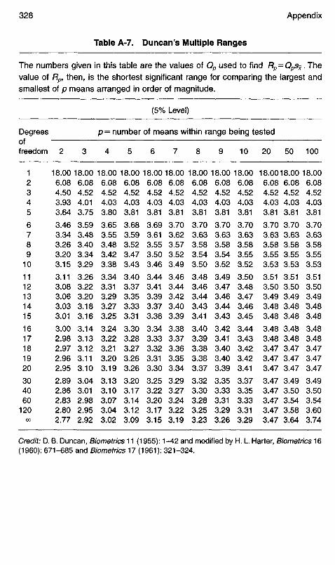
Table A-7. Duncan's Multiple Ranges
The numbers given In this table are the values of Qp used to find Rp=QpSx . Thevalue of Rp, then, is the shortest significant range for comparing the largest andsmallest of p means arranged in order of magnitude.
(5% Level)
Degreesoffreedom
12345
6789
10
1112131415
1617181920
304060
120CXO
p= number of means within range being tested
2
18.006.084.503.933.64
3.463.343.263.203.15
3.113.083.063.033.01
3.002.982.972.962.95
2.892.862.832.802.77
3
18.006.084.524.013.75
3.593.483.403.343.29
3.263.223.203.183.16
3.143.133.123.113.10
3.043.012.982.952.92
4
18.006.084.524.033.80
3.653.553.483.423.38
3.343.313.293.273.25
3.243.223.213.203.19
3.133,103.073.043.02
5
18.006.084.524.033.81
3.683.593.523.473.43
3.403.373.353.333.31
3.303.283.273.263.26
3.203.173.143.123.09
6
18.006.084.524.033.81
3.693.613.553.503.46
3.443.413.393.373.36
3.343.333.323.313.30
3.253.223.203.173.15
7
18.006.084.524.033.81
3.703.623.573.523.49
3.463.443.423.403.39
3.383.373.363.353.34
3.293.273.243.223.19
8
18.006.084.524.033.81
3.703.633.583.543.50
3.483.463.443.433.41
3.403.393.383.383.37
3.323.303.283.253.23
9
18.006.084.524.033.81
3.703.633.583.543.52
3.493.473.463.443.43
3.423.413.403.403.39
3.353.333.313.293.26
10
18.006.084.524.033.81
3.703.633.583.553.52
3.503.483.473.463.45
3.443.433.423.423.41
3.373.353.333.313.29
20
18.006.084.524.033.81
3.703.633.583.553.53
3.513.503.493.483.48
3.483.483.473.473.47
3.473.473.473.473.47
50
18.006.084.524.033.81
3.703.633.583.553.53
3.513.503.493.483.48
3.483.483.473.473.47
3.493.503.543.583.64
100
18.006.084.524.033.81
3.703.633.583.553.53
3.513.503.493.483.48
3.483.483.473.473.47
3.493.503.543.603.74
Credit: D. B. Duncan, Biometrics 1 1 (1955): 1-42 and modified by H. L. Harter, Biometrics 16(1960): 671-685 and Biometrics 17 (1961): 321-324.
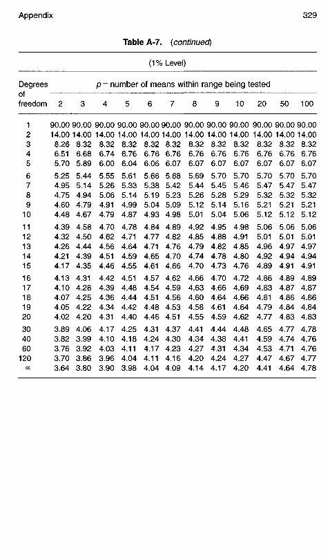
Table A-7. (continued)
(1% Level)
Degreesoffreedom
12345
6789
10
1112131415
1617181920
304060
120OO
P= number of means within range being tested
2
90.0014.008.266.515.70
5.254.954.754.604.48
4.394.324.264.214.17
4.134.104.074.054.02
3.893.823.763.703.64
3
90.0014.008.326.685.89
5.445.144.944.794.67
4.584.504.444.394.35
4.314.284.254.224.20
4.063.993.923.863.80
4
90.0014.008.326.746.00
5.555.265.064.914.79
4.704.624.564.514.46
4.424.394.364.344.31
4.174.104.033.963.90
5
90.0014.008.326.766.04
5.615.335.144.994.87
4.784.714.644.594.55
4.514.484.444.424.40
4.254.184.114.043.98
6
90.0014.008.326.766.06
5.665.385.195.044.93
4.844.774.714.654.61
4.574.544.514.484.46
4.314.244.174.114.04
7
90.0014.008.326.766.07
5.685.425.235.094.98
4.894.824.764.704.66
4.624.594.564.534.51
4.374.304.234.164.09
8
90.0014.008.326.766.07
5.695.445.265.125.01
4.924.854.794.744.70
4.664.634.604.584.55
4.414.344.274.204.14
9
90.0014.008.326.766.07
5.705.455.285.145.04
4.954.884.824.784.73
4.704.664.644.614.59
4.444.384.314.244.17
10
90.0014.008.326.766.07
5.705.465.295.165.06
4.984.914.854.804.76
4.724.694.664.644.62
4.484.414.344.274.20
20
90.0014.008.326.766.07
5.705.475.325.215.12
5.065.014.964.924.89
4.864.834.814.794.77
4.654.594.534.474.41
50
90.0014.008.326.766.07
5.705.475.325.215.12
5.065.014.974.944.91
4.894.874.864.844.83
4.774.744.714.674.64
100
90.0014.008.326.766.07
5.705.475.325.215.12
5.065.014.974.944.91
4.894.874.864.844.83
4.784.764.764.774.78
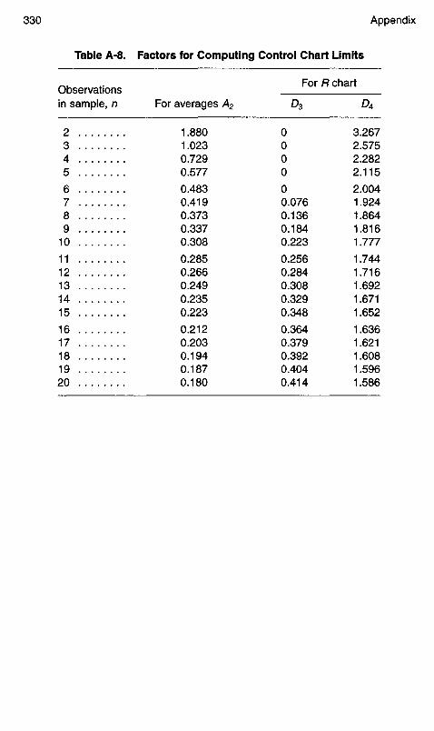
Table A-8. Factors for Computing Control Chart Limits
Observationsin sample, n
2345
6789
10
1112131415
1617181920
For averages A2
1.8801.0230.7290.577
0.4830.4190.3730.3370.308
0.2850.2660.2490.2350.223
0.2120.2030.1940.1870.180
For R chart
£3
OOOO
O0.0760.1360.1840.223
0.2560.2840.3080.3290.348
0.3640.3790.3920.4040.414
D4
3.2672.5752.2822.115
2.0041.9241.8641.8161.777
1.7441.7161.6921.6711.652
1.6361.6211.6081.5961.586

Table A-9. Military Standard 105E Sample Size Code Letters
Lot or batch size
2 to9 to
16 to
26 to51 to91 to
151 to281 to501 to
1201 to3201 to
10001 to
35001 to150001 to500001 and
81525
5090
150
280500
1200
32001000035000
150000500000over
Special inspection levels — Usedfor destructive
tests or where samplesizes must be small
S-1
AAA
ABB
BBC
CCC
DDD
S-2
AAA
BBB
CCC
DDD
EEE
S-3
AAB
BCC
DDE
EFF
GGH
S-4
AAB
CCD
EEF
GGH
JJK
General inspectionlevels — Confidence
levels
90%
I
AAB
CCD
EFG
HJK
LMN
95%
Il
ABC
DEF
GHJ
KLM
NPQ
99%
III
BCD
EFG
HJK
LMN
PQR
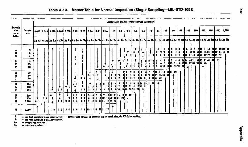
Table A-10. Master Table for Normal Inspection (Single Sampling—MIL-STD-105E
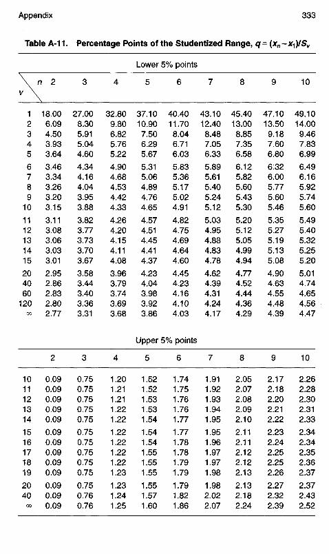
Table A-1 1 . Percentage Points of the Studentized Range, q = (xn-x^/Sv
Lower 5% points
v \
12345
6789
10
1112131415
204060
120OO
n 2
\
18.006.094.503.933.64
3.463.343.263.203.15
3.113.083.063.033.01
2.952.862.832.802.77
3
27.008.305.915.044.60
4.344.164.043.953.88
3.823.773.733.703.67
3.583.443.403.363.31
4
32.809.806.825.765.22
4.904.684.534.424.33
4.264.204.154.114.08
3.963.793.743.693.68
5
37.1010.907.506.295.67
5.315.064.894.764.65
4.574.514.454.414.37
4.234.043.983.923.86
6
40.4011.708.046.716.03
5.835.365.175.024.91
4.824.754.694.644.60
4.454.234.164.104.03
7
43.1012.408.487.056.33
5.895.615.405.245.12
5.034.954.884.834.78
4.624.394.314.244.17
8
45.4013.008.857.356.58
6.125.825.605.435.30
5.205.125.054.994.94
4.774.524.444.364.29
9
47.1013.509.187.606.80
6.326.005.775.605.46
5.355.275.195.135.08
4.904.634.554.484.39
10
49.1014.009.467.836.99
6.496.165.925.745.60
5.495.405.325.255.20
5.014.744.654.564.47
Upper 5% points
1011121314
1516171819
2040
OO
2
0.090.090.090.090.09
0.090.090.090.090.09
0.090.090.09
3
0.750.750.750.750.75
0.750.750.750.750.75
0.750.760.76
4
1.201.211.211.221.22
1.221.221.221.221.23
1.231.241.25
5
1.521.521.531.531.54
1.541.541.551.551.55
1.551.571.60
6
1.741.751.761.761.77
1.771.781.781.791.79
1.791.821.86
7
1.911.921.931.941.95
1.951.961.971.971.98
1.982.022.07
8
2.052.072.082.092.10
2.112.112.122.122.13
2.132.182.24
9
2.172.182.202.212.22
2.232.242.252.252.26
2.272.322.39
10
2.262.282.302.312.33
2.342.342.352.362.37
2.372.432.52

Table A-12. Table of a (Producer's Risk at 5%)
CfNx
68
101520304060
120OO
/C =N
2
1.731.631.581.511.481.441.431.411.401.39
3
2.592.392.292.162.102.042.011.981.951.93
4
2.942.712.582.422.352.282.252.212.182.15
5
3.192.922.782.602.522.442.402.362.332.29
6
3.373.092.932.742.642.562.522.482.442.40
8
3.333.152.932.832.732.692.642.602.55
10
3.313.072.962.862.802.762.712.65
15
3.323.183.063.002.942.882.82
20
3.333.193.133.063.002.94
30
3.373.293.223.153.08
k= number of means being compared.df = degrees of freedom in estimate of error variance, sf = of .

References
Alvarez, R. J. 1994. Managing total quality in foodservice. Food Technology 48(9):140-143.
American Institute of Baking. 1988. Quality assurance manual for food processors.Marbottam. KS: AIB.
American National Standards Institute. 1981. ANSLASQC ZI.4, Military Standard 105D.Sampling procedures and tables for inspection by attributes. New York: AmericanStandards Association.
American Society for Quality Control. 1986. Food processing industry quality systemguidelines. Milwaukee, WI: ASQC.
American Society for Testing and Materials. 1968. Basic Principles of sensory evaluation.ASTM Special Technical Publication # 433. Philadelphia, PA: ASTM., 1977. Manual on sensory testing methods. Philadelphia, PA: ASTM.
American Society for Quality Control. Tl5 1, 1986. Food processing industry qualitysystem guidelines.
American Supplier Institute. 1990. Total quality management Dearborn, MI: AmericanSupplier Institute.
ASM International (formerly American Society for Metals). Metals handbook. 8th ed.Vol. 11. Metals Park. OH: ASM International.
Boclens, and Haring 1982. Paper presented at the annual meeting of the Institute of FoodTechnologists.
Box. G. J. S. Hunter, and W. G. Hunter. 1978. Statistics for experiments. New York: Wiley.Box. G., and N. R. Draper. 1969. Evolutionary operation. New York: Wiley.Braverman, D. 1981. Fundamentals of statistical quality control.Centers for Disease Control. 1981. Foodborne disease outbreaks Atlanta, GAL CDC.Cianfrani, C., J. Tsiakals, and J. West. 2000. ISO 9001:2000 Explained. ISBN 0-87389-
508-8. Quality Press.Crosby, P. 1979. Quality is free. New York: McGraw-Hill.Dambolenn, L, and A. Rao, 1994. What is six sigma anyway? Quality. 33(1): 10.DataMyte Corporation. 1987. DataMyte handbook. Minretonka, MN: DataMyte
Corporation.Deming, S. N., and S. L. Morgan. 1988. Experimental design: A cherometric approach
New York: Elsevier.
Deming, W. E. 1975. On some statistical aids toward economic production. Interfaces5 (The Institute of Management Science) 4, 1982, Quality, productivity, and competitive position. Cambridge, MA: MIT Centerfor Advanced Engineering Study., 1986, Out of the crisis, Cambridge, MA: MIT Press.
Dodge, H. F. 1943. Administration of a sampling inspection plan. Industrial QualityControl 5(3): 12-19.
Feigenbaum, A. V 1983. Total quality control, engineering and management. 3rd ed. NewYork: McGraw-Hill.
Food and Drug Administration. 1989. Code of Federal Regulations 21, Section 101, 105.Washington, DC: Government Printing Office.
Food Processors Institute. 1982. Practical net weight control. Washington, DC: FPI.Ford Motor Company, 1985. Continuing process control and process capability improve-
ment. Plymouth, MI: Ford Motor Company.Freedman, W 1984. Products liability, New York: Van Nostrand Reinhold.Grant, E. L., and R. S. Leavenworth. 1988. Statistical quality control. 6th ed. New York:
McGraw-Hill.Grocery Manufacturers of America. 1974. Guidelines for product recall. Washington, DC:
GMA.Hansen, B. 1952. Quality control theory and applications. New York: Wiley.Heckel, J. 1988. Built in quality at Greely. Quality 27:20.Hertz, P. 1987. The Deming method, Quality, pp. Q-32-34.Hradesky, J. L. 1988. Productivity quality improvement. New York: McGraw-Hill.Hubbard, M. R. 1987. New quality control techniques for the food industry. Hornblower
39(5): 8-10.Institute of Food Technologists, Sensory Evaluation Division, 1981 Sensory evaluation
guide for testing food Food Technology November: 50.Ishikawa, K. 1982. Guide to quality control. Tokyo: Asian Productivity Center.——, 1985. What is total quality control? Englewood Cliffs, NJ: Prentice-Hall.Juran, J. M. 1988. Quality control handbook. New York: McGraw-Hill.Juran, J. M., and F. M. Gryna. 1970. Quality planning and analysis. 2nd ed. New York:
McGraw-Hill.Kennedy, C. W, and D. E. Andrews. 1987. Inspection and gaging. 5th ed. New York:
Industrial Press.McGonnagle, WJ. 1971. Nondestructive testing. New York: Gordon and Breech.Merrill Lynch. 1995. Global Investment Strategy. March 21.Mikel, H., and R. Schroeder. 2000. Six sigma. ISBN 0-385-49437-8. Doubleday.Miller, J. C., and J. N. Miller. 1988. Statistics for analytical chemistry. New York: Wiley
(Halsted).National Institute of Standards and Technology (formerly National Bureau of Standards).
1988. Handbook 133. 3rd ed., with Supplements 1,2, and 3, dated 1990, 1991, and1992. Checking the net contents of packaged goods. Washington, DC: GovernmentPrinting Office., 1995. Handbook 130, Uniform laws and regulations. Washington, DC: GovernmentPrinting Office.
Ott, E. 1975. Process and control: Trouble-shooting and interpretation of data. New York:McGraw-Hill.
Pande, P., R. Neuman, and R. Cavanagh. 2000. The six sigma way, ISVN 0-07-135806-4.New York, McGraw-Hill.

Peters, T., and R. H. Waterman, Jr. 1982. In search of excellence. New York: Harper &Row.
Pierson, M. D., and D. A. Corlett. 1992. HACCP principles and applications. New York:Chapman & Hall.
Quality Progress. 1990. The tools of quality. June through December.Rickmers, A. D., and H. N. Todd. 1967. Statistics: An introduction. New York: McGraw-
Hill.Schilling, E. G. Statistical quality control. 6th ed. New York: McGraw-Hill.Tadikamalla, P. R. 1994. The confusion over six-sigma quality. Quality Progress 27(11):
83-91.U.S. Department of Agriculture, Food Safety and Quality Service, 1988. Code of Federal
Regulations 9, Section 317.2. Washington, DC: Government Printing Office.U.S. General Accounting Office. 1991. Management Practices. GAO/NSLAD-91-190.University of Iowa ASQC Section 1303. 1965. Quality control training manual. 2nd ed.
Iowa City. IA: University of Iowa.. 1986. Statistical quality control handbook. Iowa City, IA: University of Iowa.

339 This page has been reformatted by Knovel to provide easier navigation.
Index
Index terms Links
A Acceptable Quality Level 135 150 276
Acceptance testing 39
Accuracy 12 26 38 43 120 121 178 192 321
Administration 12 134 152 154 259
Alpha risk 154
Alternate hypothesis 95
American Society for Quality 28
Analysis of variance 3 105 190 191 232 248
difference testing 108 109 one-way classification 193
ANOVA (see analysis of variance)
AQL 135
Areas under the curve 84
Artificial intelligence (see computer)
ASQC 131 149 335
ASTM 335
Attribute charts 52 57 178 290 sampling plans 115
Audits 17 20 26 121 143 264 274
B Baldridge award 27 28 290
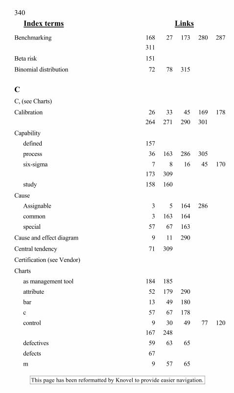
340 Index terms Links
This page has been reformatted by Knovel to provide easier navigation.
Benchmarking 168 27 173 280 287 311
Beta risk 151
Binomial distribution 72 78 315
C C, (see Charts)
Calibration 26 33 45 169 178 264 271 290 301
Capability defined 157 process 36 163 286 305 six-sigma 7 8 16 45 170
173 309 study 158 160
Cause Assignable 3 5 164 286 common 3 163 164 special 57 67 163
Cause and effect diagram 9 11 290
Central tendency 71 309
Certification (see Vendor)
Charts as management tool 184 185 attribute 52 179 290 bar 13 49 180 c 57 67 178 control 9 30 49 77 120
167 248 defectives 59 63 65 defects 67 m 9 57 65

341 Index terms Links
This page has been reformatted by Knovel to provide easier navigation.
Charts (Continued) mu 52 np 52 57 59 65 67 percent defective 52 57 211 215 pie 51 R 52 three-dimensional 49 X-bar 3 10 51 178
Chart patterns abnormal uniform 181 excessive variability 182 high/low 183 184 interpreting 64 205 296 normal 58 random cycles 180 recurring cycles 181 182 trend 9 181 uniform 181 wild outliers 183
Check sheet 9 143 290
Checkweigher 120 184 208 302 303
Chi square distribution 78
CIM. See computer
Compliance 19 20 36 169 201 204
Computer 289 activator 301 302 advantages 246 288 290 296 298 artificial intelligence 289 293 automatic control 301 302 bar codes 298 controlled processing 289 299
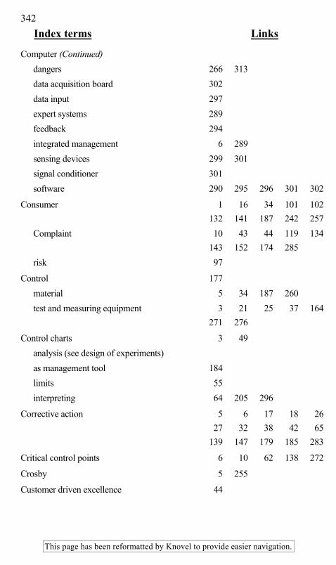
342 Index terms Links
This page has been reformatted by Knovel to provide easier navigation.
Computer (Continued) dangers 266 313 data acquisition board 302 data input 297 expert systems 289 feedback 294 integrated management 6 289 sensing devices 299 301 signal conditioner 301 software 290 295 296 301 302
Consumer 1 16 34 101 102 132 141 187 242 257
Complaint 10 43 44 119 134 143 152 174 285
risk 97
Control 177 material 5 34 187 260 test and measuring equipment 3 21 25 37 164
271 276
Control charts 3 49 analysis (see design of experiments) as management tool 184 limits 55 interpreting 64 205 296
Corrective action 5 6 17 18 26 27 32 38 42 65 139 147 179 185 283
Critical control points 6 10 62 138 272
Crosby 5 255
Customer driven excellence 44

343 Index terms Links
This page has been reformatted by Knovel to provide easier navigation.
D Data control 260
input (see computer)
Defectives 22 52 58 77
Defects classes 132 133 259 classification 132 critical few 134 trivial many 134
Delivery 21 24 126 137 159
256 263 266 271 272 280 304
Deming 3 4 46 164 174 278 282 309 312 313
cycle, (see Plan/Do/Check/Act)
Design assurance 17
Design of experiments 9 219 220 286 290 central composite 236 237 242 243 control chart analysis 138 248 experimental variables 222 252 external variables 221 extraneous variables 221 225 fractional factorial 227 232 290 full factorial 227 goal 4 28 40 130 173
183 219 272 282 incomplete block 224 225 244 interaction effect 228 Latin square 220 224 mixture 189 193 227 239

344 Index terms Links
This page has been reformatted by Knovel to provide easier navigation.
Design of experiments (Continued) response surface 9 227 236 242 246
247 review 17 24 star points 237 243
Difference testing 108 109 193
Dispersion 71 92 106 107 221
Distribution binomial 77 90 91 316 difference between means 100 101 109 251 F 78 104 105 325 normal 77 81 92 97 283
290 Poisson 80 81 90 sample means 80 105 t 16 17 92 93 100
101 117 206 208 322
Document control 38 20
Documentation 18 25 27 33 34 139 145 147 269 270
Duncan’s Multiple Range Test 108 109 251 252
E Education 4 18 23 264 278
312
Equipment 3 18 30 135 213 259 278
Evolutionary operations (see EVOP)
EVOP 11 222
Experiment. See Design of experiments.
Experimental error 107 223 236
Expert systems (see computer)

345 Index terms Links
This page has been reformatted by Knovel to provide easier navigation.
F F-distribution 77 78 104 105 325
327
Factorial design (see Design of experiments)
FDA 6 19 20 34 36 46 134 138 159 259 271
Federal agencies 15
Fiegenbaum 4 163 226
Finished product: testing 38 39
Flow chart 8 22 144 283 302 303
Food processing industry quality system guide-lines 15
Food quality systems 15
Frequency 5 9 13 32 36 74 75 77 82 83 96 115 120 137 138 141 142 145 149 189 192 267 283 290 305
G Goals 4 7 16 22 28
34 35 40 57 118 135 174 201 213 221 260 262 272 277 282 283 298 312
Good manufacturing practice 18 20 30 36 141 148 150 201 271 272
Gross domestic product 1

346 Index terms Links
This page has been reformatted by Knovel to provide easier navigation.
H HAACP 16 138 145 283 287
337
Handbook packaged goods 202 204 209
Handling and production functions 17 19 25 39 62 204 226 259 268 269 290
Health and Human Services 6 201
Histogram 9 75 90 283 290 296
Hypothesis 95 102 105 290
I Implementing quality program 275
hardware industry 25 in-house 152 192 277 287 288 management commitment 5 20 22 275 PDCA cycle 282 professional training 290 teams 20 30 266 293 298
312 training technicians 287 288
Imports 1
Incomplete block 224 225 244
Inspection 4 and test status 24 and testing 24 257 equipment 24
Internal audits 26
Ishikawa 11 256 ISO 9000 6 17 20 26 32
272 291

347 Index terms Links
This page has been reformatted by Knovel to provide easier navigation.
J JIT 265
Juran 4 163 278 337
Just in time (see JIT)
L Latin square 223
Leadership through quality 28
Least significant difference 124
Lot size 58 62 136 149
M m charts 57 65
Malcolm Baldridge 7 27
Management: commitment 5 275 control 45 responsibility 20
Manual 21 22 31 32 47 287
HACCP 146
Manufacturing operations 19
MAV 202 203 214 (see also Net content control)
Mean 71 84 100
Median 71 73
Methods and standards 33
MilStd 105E 132 149 332
Motivation 47

348 Index terms Links
This page has been reformatted by Knovel to provide easier navigation.
N Net content control 201
categories 202 evaluation 205 208 217 regulations 201 risk analysis 210 212 setting fill targets 213 (see also Handbook)
Non-conforming product 20
Noncomformity 20 267
Normal distribution 77 61 92 97 283
np 57 80 315
Null hypothesis 95 96 98 101
O Odor 188 189
Operations: proprietary 37 160
Operator control 45
P p charts 52 180 184
Packaging supplier quality assurance 30 265
Paired observations 100
Panels selection 195 training 197 types 194
Parameter 84
Pareto chart 9 12 13
Partitioning sum of squares 106
PDCA 282 (see Plan/Do/Check/Act)

349 Index terms Links
This page has been reformatted by Knovel to provide easier navigation.
Pearce, S 17
Percent defective 52 57 211 215
Personnel 15 23 36 136 191 275 293
Peters 5
Pie charts 51
Plan/Do/Check/Act 28 282 313
Plant 16 117
Poisson distribution 80
Policy 30 41 45 217 218
Precision 55 221
Preventive action 27
Probability 26 76 77 80 95 96
Process capability 5 157
study 36 167 168 178 control 18 177 299
(also see computer) drift 116 168 169 flow diagram 139 140 282 283
Processes 18
Product Coding 38 259 271 performance 42 research and development 33 safety and liability 43 verification 20 25 37 38
Production quality control 36 117
Purchased goods (see Vendor)

350 Index terms Links
This page has been reformatted by Knovel to provide easier navigation.
Purchasing materials 17 18 62 140 183
219 257 supplies 10 57 263 266
Q Quality
authorities 34 control programs 3 control tools 8 documentation and records 40 goal of R&D 33 goals 4 34 40 201 221
260 262 282 improvement 4 26 280 improvement process 33 in marketing 33 in production 17 32 36 289 leadership 4 21 27 28 personnel 36 40 46 47 184
185 222 277 policies 4 47 programs 5 8 proud program 28 records 39 40 264 strategies 28 system guidelines 16 45 335
Quality: system 15 121 279
Quality control manual 20 31 32 287 production 17 28 32 36

351 Index terms Links
This page has been reformatted by Knovel to provide easier navigation.
R R charts 53 183 218
Randomized block 222
Range control 177 Duncan multiple 108 109 exaggerated 72 73 procedure 54
Raw materials 257 258
Recall 39 45 46 336
Records retention 40
Records: quality 39 40
Relationships 39 40
Reports: progress 34
Response surface (see Design of experiments)
Reviews 22 34 45 169
Risk alpha 135 136 beta 135 consumer 135 minimum 214 producer 135 sampling 135 Type I 135 Type II 135
S Sampling 115
attribute sampling 149 150 cluster 127 128 constant percentage 121 different distributions 117

352 Index terms Links
This page has been reformatted by Knovel to provide easier navigation.
Sampling (Continued) double 131 150 frequency 120 location 5 270 287 multiple 131 149 150 100 percent 119 261 parameters 115 plans 6 9 77 80 115
128 131 135 149 150 202 272
procedures 116 123 131 149 259 335
risks 135 149 selection 128 137 138 184 simple random 123 single 68 131 139 177 190
191 size 32 55 64 78 84
90 106 115 118 128 136 149 150 203 248 331
spot checking 121 square root 69 73 121 172 statistical 123 stratified 126 127 systematic 124 125 types 128
Sanitary facilities 18 19
Sanitary operations 17
Scatter diagram 9
Sensors 299

353 Index terms Links
This page has been reformatted by Knovel to provide easier navigation.
Sensory testing cold 189 general 188 heat 19 189 odor 188 189 pain 190 sight 189 sound 189 taste 189 touch 189 type 191 192 (see also Panels)
Servicing 7 28
Shewhart 3 58
Software (see computer)
Specifications ingredients 157 process 31 160 161 177 product 157
SQC techniques 10 138
Standard deviation 45 72 78 83 89 92 100 101 104 109 167 172 213 252
Standards 6 16 20 33 131 132 134 149 154 183 194 202 258 259 311 331 336
Star points (see design of experiments)
Statistics 85 336 337 methods 3 26 153 software (see computer) techniques 9 10 287

354 Index terms Links
This page has been reformatted by Knovel to provide easier navigation.
Storage 18 19 25 39 187 193 194
Supplier certification (see Vendor)
Systems: food quality 15 guidelines 15
T t-distribution 78 92 93 100 101
322
Taste 188 189 192 193 198
Teams 30 277 312 quality systems 28 30
Test equipment: calibration 37 38
Testing basic library 152 equipment 3 25 27 38 271 methods 33 189 335 packaging 266 rapid analyses 155 references 151 335 sensory 153 187 335 336
Tools basic 9 selection 8
Total quality commitment 21 22 28 management 275 service 28 systems 28
TQM: definition 28
Training 4 16 21 45 168 195 275 291 337

355 Index terms Links
This page has been reformatted by Knovel to provide easier navigation.
Two criteria classification 111
Type I risk 135 136
Type II risk 136
U Universal way 28
Unpaired observations 116
USDA 34 134 138 203 271 272
User contact 16 18
Utensils 18
V Variability 2 92 134 169 182
221
Variables design 223 examples 129 outcome 220 223 233 236 240 response 221 223 227 233 239
241 247
Variance 72 73 78 105 190 191 232 248 291
Vendor certification 256 266 Ishikawa 11 256 262 336 JIT 265 materials specifications 17 34 254 257 quality 253 price 263 records 270 selection 35 263 264

356 Index terms Links
This page has been reformatted by Knovel to provide easier navigation.
Vendor (Continued) single source 265 vendor-vendee relations 255
W Warehousing 19 146 267
Weibull distribution 78
Weight control (see Net content control)
X X-Bar charts 3 52 180 218
Z Z 83