statistical physics - ethedu.itp.phys.ethz.ch/hs12/statphys/notes-sp-hs12-complete.pdf ·...
TRANSCRIPT

Statistical Physics
ETH Zurich – Herbstsemester 2012
Manfred Sigrist, HIT K23.8Tel.: 3-2584, Email: [email protected]
Webpage: http://www.itp.phys.ethz.ch/research/condmat/strong/
Literature:
• Statistical Mechanics, K. Huang, John Wiley & Sons (1987).
• Introduction to Statistical Physics, K. Huang, Chapman & Hall Books (2010).
• Equilibrium Statistical Physics, M. Plischke and B. Bergersen, Prentice-Hall International(1989).
• Theorie der Warme, R. Becker, Springer (1978).
• Thermodynamik und Statistik, A. Sommerfeld, Harri Deutsch (1977).
• Statistische Physik, Vol. V, L.D. Landau and E.M Lifschitz, Akademie Verlag Berlin(1975).
• Statistische Mechanik, F. Schwabl, Springer (2000).
• Elementary Statistical Physics, Charles Kittel,John Wiley & Sons (1967).
• Statistical Mechanics, R.P. Feynman, Advanced Book Classics, Perseus Books (1998).
• Statistische Mechanik, R. Hentschke, Wiley-VCH (2004).
• Introduction to Statistical Field Theory, E. Brezin, Cambridge (2010).
• Statistical Mechanics in a Nutshell, Luca Peliti, Princeton University Press (2011).
• Principle of condensed matter physics, P.M. Chaikin and T.C. Lubensky, Cambridge Uni-versity Press (1995).
• Many other books and texts mentioned throughout the lecture
Lecture Webpage:
http://www.itp.phys.ethz.ch/education/lectures hs12/StatPhys
1

Contents
1 Laws of Thermodynamics 51.1 State variables and equations of state . . . . . . . . . . . . . . . . . . . . . . . . 5
1.1.1 State variables . . . . . . . . . . . . . . . . . . . . . . . . . . . . . . . . . 51.1.2 Temperature as an equilibrium variable . . . . . . . . . . . . . . . . . . . 71.1.3 Equation of state . . . . . . . . . . . . . . . . . . . . . . . . . . . . . . . . 71.1.4 Response function . . . . . . . . . . . . . . . . . . . . . . . . . . . . . . . 8
1.2 First Law of Thermodynamics . . . . . . . . . . . . . . . . . . . . . . . . . . . . . 81.2.1 Heat and work . . . . . . . . . . . . . . . . . . . . . . . . . . . . . . . . . 81.2.2 Thermodynamic transformations . . . . . . . . . . . . . . . . . . . . . . . 91.2.3 Applications of the first law . . . . . . . . . . . . . . . . . . . . . . . . . . 10
1.3 Second law of thermodynamics . . . . . . . . . . . . . . . . . . . . . . . . . . . . 101.3.1 Carnot engine . . . . . . . . . . . . . . . . . . . . . . . . . . . . . . . . . . 111.3.2 Entropy . . . . . . . . . . . . . . . . . . . . . . . . . . . . . . . . . . . . . 121.3.3 Applications of the first and second law . . . . . . . . . . . . . . . . . . . 13
1.4 Thermodynamic potentials . . . . . . . . . . . . . . . . . . . . . . . . . . . . . . 141.4.1 Legendre transformation to other thermodynamical potentials . . . . . . . 151.4.2 Homogeneity of the potentials . . . . . . . . . . . . . . . . . . . . . . . . . 161.4.3 Conditions for the equilibrium states . . . . . . . . . . . . . . . . . . . . . 17
1.5 Third law of thermodynamics . . . . . . . . . . . . . . . . . . . . . . . . . . . . . 18
2 Kinetic approach and Boltzmann transport theory 202.1 Time evolution and Master equation . . . . . . . . . . . . . . . . . . . . . . . . . 20
2.1.1 H-function and information . . . . . . . . . . . . . . . . . . . . . . . . . . 222.1.2 Simulation of a two-state system . . . . . . . . . . . . . . . . . . . . . . . 232.1.3 Equilibrium of a system . . . . . . . . . . . . . . . . . . . . . . . . . . . . 25
2.2 Analysis of a closed system . . . . . . . . . . . . . . . . . . . . . . . . . . . . . . 262.2.1 H and the equilibrium thermodynamics . . . . . . . . . . . . . . . . . . . 262.2.2 Master equation . . . . . . . . . . . . . . . . . . . . . . . . . . . . . . . . 272.2.3 Irreversible processes and increase of entropy . . . . . . . . . . . . . . . . 28
2.3 Boltzmann’s kinetic gas and transport theory . . . . . . . . . . . . . . . . . . . . 312.3.1 Statistical formulation . . . . . . . . . . . . . . . . . . . . . . . . . . . . . 312.3.2 Collision integral . . . . . . . . . . . . . . . . . . . . . . . . . . . . . . . . 332.3.3 Collision conserved quantities . . . . . . . . . . . . . . . . . . . . . . . . . 342.3.4 Boltzmann’s H-theorem . . . . . . . . . . . . . . . . . . . . . . . . . . . . 34
2.4 Maxwell-Boltzmann-Distribution . . . . . . . . . . . . . . . . . . . . . . . . . . . 352.4.1 Equilibrium distribution function . . . . . . . . . . . . . . . . . . . . . . . 352.4.2 Relation to equilibrium thermodynamics - dilute gas . . . . . . . . . . . . 372.4.3 Local equilibrium state . . . . . . . . . . . . . . . . . . . . . . . . . . . . 38
2.5 Fermions and Bosons . . . . . . . . . . . . . . . . . . . . . . . . . . . . . . . . . . 392.6 Transport properties . . . . . . . . . . . . . . . . . . . . . . . . . . . . . . . . . . 40
2.6.1 Relaxation time approximation . . . . . . . . . . . . . . . . . . . . . . . . 402.7 Electrical conductivity of an electron gas . . . . . . . . . . . . . . . . . . . . . . . 42
2

3 Classical statistical Physics 453.1 Gibbsian concept of ensembles . . . . . . . . . . . . . . . . . . . . . . . . . . . . 45
3.1.1 Liouville Theorem . . . . . . . . . . . . . . . . . . . . . . . . . . . . . . . 463.1.2 Equilibrium system . . . . . . . . . . . . . . . . . . . . . . . . . . . . . . . 47
3.2 Microcanonical ensemble . . . . . . . . . . . . . . . . . . . . . . . . . . . . . . . . 483.2.1 Entropy . . . . . . . . . . . . . . . . . . . . . . . . . . . . . . . . . . . . . 483.2.2 Relation to thermodynamics . . . . . . . . . . . . . . . . . . . . . . . . . 50
3.3 Discussion of ideal systems . . . . . . . . . . . . . . . . . . . . . . . . . . . . . . 503.3.1 Classical ideal gas . . . . . . . . . . . . . . . . . . . . . . . . . . . . . . . 503.3.2 Ideal paramagnet . . . . . . . . . . . . . . . . . . . . . . . . . . . . . . . . 52
3.4 Canonical ensemble . . . . . . . . . . . . . . . . . . . . . . . . . . . . . . . . . . . 543.4.1 Thermodynamics . . . . . . . . . . . . . . . . . . . . . . . . . . . . . . . . 553.4.2 Equipartition law . . . . . . . . . . . . . . . . . . . . . . . . . . . . . . . . 563.4.3 Fluctuation of the energy and the equivalence of microcanonial and canon-
ical ensembles . . . . . . . . . . . . . . . . . . . . . . . . . . . . . . . . . . 583.4.4 Ideal gas in canonical ensemble . . . . . . . . . . . . . . . . . . . . . . . . 593.4.5 Ideal paramagnet . . . . . . . . . . . . . . . . . . . . . . . . . . . . . . . . 593.4.6 More advanced example - classical spin chain . . . . . . . . . . . . . . . . 61
3.5 Grand canonical ensemble . . . . . . . . . . . . . . . . . . . . . . . . . . . . . . . 653.5.1 Relation to thermodynamics . . . . . . . . . . . . . . . . . . . . . . . . . 663.5.2 Ideal gas . . . . . . . . . . . . . . . . . . . . . . . . . . . . . . . . . . . . . 673.5.3 Chemical potential in an external field . . . . . . . . . . . . . . . . . . . . 683.5.4 Paramagnetic ideal gas . . . . . . . . . . . . . . . . . . . . . . . . . . . . . 68
4 Quantum Statistical Physics 704.1 Basis of quantum statistics . . . . . . . . . . . . . . . . . . . . . . . . . . . . . . 704.2 Density matrix . . . . . . . . . . . . . . . . . . . . . . . . . . . . . . . . . . . . . 714.3 Ensembles in quantum statistics . . . . . . . . . . . . . . . . . . . . . . . . . . . 72
4.3.1 Microcanonical ensemble . . . . . . . . . . . . . . . . . . . . . . . . . . . . 724.3.2 Canonical ensemble . . . . . . . . . . . . . . . . . . . . . . . . . . . . . . 724.3.3 Grandcanonical ensemble . . . . . . . . . . . . . . . . . . . . . . . . . . . 734.3.4 Ideal gas in grandcanonical ensemble . . . . . . . . . . . . . . . . . . . . . 73
4.4 Properties of Fermi gas . . . . . . . . . . . . . . . . . . . . . . . . . . . . . . . . 754.4.1 High-temperature and low-density limit . . . . . . . . . . . . . . . . . . . 764.4.2 Low-temperature and high-density limit: degenerate Fermi gas . . . . . . 774.4.3 Spin-1/2 Fermions in a magnetic field . . . . . . . . . . . . . . . . . . . . 78
4.5 Bose gas . . . . . . . . . . . . . . . . . . . . . . . . . . . . . . . . . . . . . . . . . 794.5.1 Bosonic atoms . . . . . . . . . . . . . . . . . . . . . . . . . . . . . . . . . 794.5.2 High-temperature and low-density limit . . . . . . . . . . . . . . . . . . . 804.5.3 Low-temperature and high-density limit: Bose-Einstein condensation . . . 80
4.6 Photons and phonons . . . . . . . . . . . . . . . . . . . . . . . . . . . . . . . . . 844.6.1 Blackbody radiation - photons . . . . . . . . . . . . . . . . . . . . . . . . 854.6.2 Phonons in a solid . . . . . . . . . . . . . . . . . . . . . . . . . . . . . . . 87
4.7 Diatomic molecules . . . . . . . . . . . . . . . . . . . . . . . . . . . . . . . . . . . 89
5 Phase transitions 925.1 Ehrenfest classification of phase transitions . . . . . . . . . . . . . . . . . . . . . 925.2 Phase transition in the Ising model . . . . . . . . . . . . . . . . . . . . . . . . . . 94
5.2.1 Mean field approximation . . . . . . . . . . . . . . . . . . . . . . . . . . . 945.2.2 Instability of the paramagnetic phase . . . . . . . . . . . . . . . . . . . . 955.2.3 Phase diagram . . . . . . . . . . . . . . . . . . . . . . . . . . . . . . . . . 985.2.4 Gaussian transformation . . . . . . . . . . . . . . . . . . . . . . . . . . . . 100
3

5.2.5 Correlation function and susceptibility . . . . . . . . . . . . . . . . . . . . 1015.3 Ginzburg-Landau theory . . . . . . . . . . . . . . . . . . . . . . . . . . . . . . . . 104
5.3.1 Ginzburg-Landau theory for the Ising model . . . . . . . . . . . . . . . . 1045.3.2 Critical exponents . . . . . . . . . . . . . . . . . . . . . . . . . . . . . . . 1065.3.3 Range of validity of the mean field theory - Ginzburg criterion . . . . . . 107
5.4 Self-consistent field approximation . . . . . . . . . . . . . . . . . . . . . . . . . . 1085.4.1 Renormalization of the critical temperature . . . . . . . . . . . . . . . . . 1085.4.2 Renormalized critical exponents . . . . . . . . . . . . . . . . . . . . . . . . 109
5.5 Long-range order - Peierls’ argument . . . . . . . . . . . . . . . . . . . . . . . . . 1115.5.1 Absence of finite-temperature phase transition in the 1D Ising model . . . 1115.5.2 Long-range order in the 2D Ising model . . . . . . . . . . . . . . . . . . . 111
6 Linear Response Theory 1136.1 Linear Response function . . . . . . . . . . . . . . . . . . . . . . . . . . . . . . . 113
6.1.1 Kubo formula - retarded Green’s function . . . . . . . . . . . . . . . . . . 1146.1.2 Information in the response function . . . . . . . . . . . . . . . . . . . . . 1156.1.3 Analytical properties . . . . . . . . . . . . . . . . . . . . . . . . . . . . . . 1166.1.4 Fluctuation-Dissipation theorem . . . . . . . . . . . . . . . . . . . . . . . 117
6.2 Example - Heisenberg ferromagnet . . . . . . . . . . . . . . . . . . . . . . . . . . 1196.2.1 Tyablikov decoupling approximation . . . . . . . . . . . . . . . . . . . . . 1206.2.2 Instability condition . . . . . . . . . . . . . . . . . . . . . . . . . . . . . . 1216.2.3 Low-temperature properties . . . . . . . . . . . . . . . . . . . . . . . . . . 122
7 Renormalization group 1237.1 Basic method - Block spin scheme . . . . . . . . . . . . . . . . . . . . . . . . . . 1237.2 One-dimensional Ising model . . . . . . . . . . . . . . . . . . . . . . . . . . . . . 1257.3 Two-dimensional Ising model . . . . . . . . . . . . . . . . . . . . . . . . . . . . . 127
A 2D Ising model: Monte Carlo method and Metropolis algorithm 131A.1 Monte Carlo integration . . . . . . . . . . . . . . . . . . . . . . . . . . . . . . . . 131A.2 Monte Carlo methods in thermodynamic systems . . . . . . . . . . . . . . . . . . 131A.3 Example: Metropolis algorithm for the two site Ising model . . . . . . . . . . . . 132
B High-temperature expansion of the 2D Ising model: Finding the phase tran-sition with Pade approximants 135B.1 High-temperature expansion . . . . . . . . . . . . . . . . . . . . . . . . . . . . . . 135B.2 Finding the singularity with Pade approximants . . . . . . . . . . . . . . . . . . . 137
4

Chapter 1
Laws of Thermodynamics
Thermodynamics is a phenomenological, empirically derived, macroscopic description of theequilibrium properties of physical systems with enormously many particles or degrees of freedom.These systems are usually considered big enough such that the boundary effects do not play animportant role (we call this the ”thermodynamic limit”). The macroscopic states of such systemscan be characterized by several macroscopically measurable quantities whose mutual relation canbe cast into equations and represent the theory of thermodynamics.
Much of the body of thermodynamics has been developed already in the 19th century beforethe microscopic nature of matter, in particular, the atomic picture has been accepted. Thus,the principles of thermodynamics do not rely on the input of such specific microscopic details.The three laws of thermodynamics constitute the essence of thermodynamics.
1.1 State variables and equations of state
Equilibrium states described by thermodynamics are states which a system reaches after a longwaiting (relaxation) time. Macroscopically systems in equilibrium do not show an evolution intime. Therefore time is not a variable generally used in thermodynamics. Most of processesdiscussed are considered to be quasistatic, i.e. the system is during a change practically alwaysin a state of equilibrium (variations occur on time scales much longer than relaxation times tothe equilibrium).
1.1.1 State variables
In thermodynamics, equilibrium states of a system are uniquely characterized by measurablemacroscopic quantities, generally called state variables (or state functions). We distinguishintensive and extensive state variables.
• intensive state variable: homogeneous of degree 0, i.e. independent of system size
• extensive state variable: homogeneous of degree 1, i.e. proportional to the system size
Examples of often used state variables are:
intensive extensiveT temperature S entropyp pressure V volumeH magnetic field M magnetizationE electric field P dielectric polarizationµ chemical potential N particle number
5

Intensive and extensive variables form pairs of conjugate variables, e.g. temperature and entropyor pressure and volume, etc.. Their product lead to energies which are extensive quantities (inthe above list each line gives a pair of conjugate variables). Intensive state variables can oftenbe used as equilibrium variable. Two systems are in equilibrium with each other, if all theirequilibrium variable are identical.The state variables determine uniquely the equilibrium state, independent of the way this statewas reached. Starting from a state A the state variable Z of state B is obtained by
Z(B) = Z(A) +∫
γ1
dZ = Z(A) +∫
γ2
dZ , (1.1)
where γ1 and γ2 represent different paths in space of states (Fig. 1.1).
B
1
γ2
Z
Y
X
A
γ
Fig.1.1: Space of states: A and B are equilibrium states connected by paths γ1 or γ2. Thecoordinates X , Y and Z are state variables of the system.
From this follows for the closed path γ = γ1 − γ2:∮γdZ = 0 . (1.2)
This is equivalent to the statement that Z is an exact differential, i.e. it is single-valued in thespace of states. If we can write Z as a function of two independent state variables X and Y (seeFig.1.1) then we obtain
dZ =(∂Z
∂X
)Y
dX +(∂Z
∂Y
)X
dY with[∂
∂Y
(∂Z
∂X
)Y
]X
=[∂
∂X
(∂Z
∂Y
)X
]Y
. (1.3)
The variable at the side of the brackets indicates the variables to be fixed for the partial deriva-tive. This can be generalized to many, say n, variables Xi (i = 1, ..., n). Then n(n − 1)/2conditions are necessary to ensure that Z is an exact differential:
dZ =n∑
i=1
(∂Z
∂Xi
)Xj 6=i
dXi with
[∂
∂Xk
(∂Z
∂Xi
)Xj 6=i
]Xj 6=k
=
[∂
∂Xi
(∂Z
∂Xk
)Xj 6=k
]Xj 6=i
.
(1.4)As we will see later not every measurable quantity of interest is an exact differential. Examplesof such quantities are the different forms of work and the heat as a form of energy.
6

1.1.2 Temperature as an equilibrium variable
Temperature is used as an equilibrium variable which is so essential to thermodynamics that thedefinition of temperature is sometimes called ”0th law of thermodynamics”. Every macroscopicthermodynamic system has a temperature T which characterizes its equilibrium state. Thefollowing statements apply:
• In a system which is in its equilibrium the temperature is everywhere the same. A systemwith an inhomogeneous temperature distribution, T (~r) is not in its equilibrium (a heatcurrent proportional to ~∇T (~r) flows in order to equilibrate the system; in such a systemstate variables evolve in time).
• For two systems, A and B, which are each independently in thermal equilibrium, we canalways find the relations: TA < TB, TA > TB or TA = TB.
• The order of systems according to their temperature is transitive. We find for systems A,B and C, that TA > TB and TB > TC leads to TA > TC .
• The equilibrium state of two systems (A and B) in thermal contact is characterized byTA = TB = TA∪B. If before equilibration T ′A > T ′B, then the equilibrium temperature hasto lie between the two temperatures: T ′A > TA∪B > T ′B.
Analogous statements can be made about other intensive state variables such as pressure andthe chemical potential which are equilibrium variables.
1.1.3 Equation of state
The equilibrium state of a thermodynamic system is described completely by a set of indepen-dent state variables (Z1, Z2, . . . , Zn) which span the space of all possible states. Within thisspace we find a subspace which represents the equilibrium states and can be determined by thethermodynamic equation of state
f(Z1, . . . , Zn) = 0 . (1.5)
The equation of state can be determined from experiments or from microscopic models throughstatistical physics, as we will see later.Ideal gas: As one of the simplest examples of a thermodynamic system is the ideal gas, microscop-ically, a collection of independent identical atoms or molecules. In real gases the atoms/moleculesinteract with each other such that at low enough temperature (T < TB boiling temperature)the gas turns into a liquid. The ideal gas conditions is satisfied for real gases at temperaturesT TB.1
The equation of state is given through the Boyle-Mariotte-law (∼ 1660 - 1675) and the Gay-Lussac-law (1802). The relevant space of states consists of the variables pressure p, volume Vand temperature T and the equation of state is
pV = nRT = NkBT (1.6)
where n is the number of moles of the gas. One mole contains NA = 6.022 ·1023 particles (atomsor molecules).2 N is the number of gas particles. The gas constant R and the Boltzmannconstant kB are then related and given by
R = 8.314J
KMolor kB =
R
NA= 1.381 · 10−23 J
K. (1.7)
The temperature T entering the equation of state of the ideal gas defines the absolute temper-ature in Kelvin scale with T = 0K at −273.15C.
1Ideal gases at very low temperatures are subject to quantum effects and become ideal quantum gases whichdeviate from the classical ideal gas drastically.
2At a pressure of 1 atm = 760 Torr = 1.01 bar = 1.01 · 105 Pa (Nm−2), the volume of one mole of gas isV = 22.4 · 10−3m3.
7

T
p
V
Fig.1.2: Equilibrium states of the ideal gas in the p− V − T -space.
1.1.4 Response function
There are various measurable quantities which are based on the reaction of a system to thechange of external parameters. We call them response functions. Using the equation of statefor the ideal gas we can define the following two response functions:
isobar thermal expansion coefficient α =1V
(∂V
∂T
)p
=1T
isothermal compressibility κT = − 1V
(∂V
∂p
)T
=1p
i.e. the change of volume (a state variable) is measured in response to change in temperature Tand pressure p respectively.3 As we consider a small change of these external parameters only,the change of volume is linear: ∆V ∝ ∆T,∆p, i.e. linear response.
1.2 First Law of Thermodynamics
The first law of thermodynamics declares heat as a form of energy, like work, potential orelectromagnetic energy. The law has been formulated around 1850 by the three scientists JuliusRobert Mayer, James Prescott Joule and Hermann von Helmholtz.
1.2.1 Heat and work
In order to change the temperature of a system while fixing state variables such as pressure,volume and so on, we can transfer a certain amount of heat δQ from or to the systems by puttingit into contact with a heat reservoir of certain temperature. In this context we can define theheat capacity Cp (CV ) for fixed pressure (fixed volume),
δQ = CpdT (1.8)
Note that Cp and CV are response functions. Heat Q is not a state variable, indicated in thedifferential by δQ instead of dQ.
3”Isobar”: fixed pressure; ”isothermal”: fixed temperature.
8

The workW is defined analogous to the classical mechanics, introducing a generalized coordinateq and the generalized conjugate force F ,
δW = Fdq . (1.9)
Analogous to the heat, work is not a state variable. By definition δW < 0 means, that work isextracted from the system, it ”does” work. A form of δW is the mechanical work for a gas,
δW = −pdV , (1.10)
or magnetic workδW = HdM . (1.11)
The total amount of work is the sum of all contributions
δW =∑
i
Fidqi . (1.12)
The first law of thermodynamics may now be formulated in the following way: Each thermo-dynamic system possesses an internal energy U which consists of the absorbed heat and thework,
dU = δQ+ δW = δQ+∑
i
Fidqi (1.13)
In contrast to Q and W , U is a state variable and is conserved in an isolated system. Alternativeformulation: There is no perpetuum mobile of the first kind, i.e. there is no machine whichproduces work without any energy supply.
Ideal gas: The Gay-Lussac-experiment (1807)4 leads to the conclusion that the internal energy Uis only a function of temperature, but not of the volume or pressure, for an ideal gas: U = U(T ).Empirically or in derivation from microscopic models we find
U(T ) =
32NkBT + U0 single-atomic gas
52NkBT + U0 diatomic molecules ,
(1.14)
Here U0 is a reference energy which can be set zero. The difference for different moleculesoriginates from different internal degrees of freedom. Generally, U = f
2NkBT with f as thenumber of degrees of freedom. This is the equipartition law.5 The equation U = U(T, V, ...)is called caloric equation of state, in contrast to the thermodynamic equation of state discussedabove.
1.2.2 Thermodynamic transformations
In the context of heat and work transfer which correspond to transformations of a thermody-namic system, we introduce the following terminology to characterize such transformations:
• quasistatic: the external parameters are changed slowly such that the system is alwaysapproximatively in an equilibrium state.
4Consider an isolated vessel with two chambers separated by a wall. In chamber 1 we have a gas and chamber2 is empty. After the wall is removed the gas expands (uncontrolled) in the whole vessel. In this process thetemperature of the gas does not change. In this experiment neither heat nor work has been transfered.
5A single-atomic molecule has only the three translational degrees of freedom, while a diatomic molecule hasadditionally two independent rotational degrees of freedom with axis perpendicular to the molecule axis connectingto two atoms.
9

• reversible: a transformation can be completely undone, if the external parameters arechanged back to the starting point in the reversed time sequence. A reversible transfor-mation is always quasistatic. But not every quasistatic process is reversible (e.g. plasticdeformation).
• isothermal: the temperature is kept constant. Isothermal transformations are generallyperformed by connecting the thermodynamic system to an ”infinite” heat reservoir of giventemperature T , which provides a source or sink of heat in order to fix the temperature.
• adiabatic: no heat is transfered into or out of the system, δQ = 0. Adiabatic transforma-tions are performed by decoupling the system from any heat reservoir. Such a system isthermally isolated.
• cyclic: start and endpoint of the transformation are identical, but generally the path inthe space of state variables does not involve retracing.
1.2.3 Applications of the first law
The heat capacity of a system is determined via the heat transfer δQ necessary for a giventemperature change. For a gas this is expressed by
δQ = dU − δW = dU + pdV =(∂U
∂T
)V
dT +(∂U
∂V
)T
dV + pdV . (1.15)
The heat capacity at constant volume (dV = 0) is then
CV =(δQ
dT
)V
=(∂U
∂T
)V
. (1.16)
On the other hand, the heat capacity at constant pressure (isobar) is expressed as
Cp =(δQ
dT
)p
=(∂U
∂T
)V
+[(
∂U
∂V
)T
+ p
](∂V
∂T
)p
. (1.17)
which leads to
Cp − CV =(
∂U
∂V
)T
+ p
(∂V
∂T
)p
=(
∂U
∂V
)T
+ p
V α . (1.18)
Here α is the isobar thermal expansion coefficient. For the ideal gas, we know that U does notdepend on V . With the equation of state we obtain(
∂U
∂V
)T
= 0 and(∂V
∂T
)p
=nR
p⇒ Cp − CV = nR = NkB . (1.19)
As a consequence it is more efficient to change the temperature of a gas by heat transfer at con-stant volume, because for constant pressure some of the heat transfer is turned into mechanicalwork δW = −p dV .
1.3 Second law of thermodynamics
While the energy conservation stated in the first law is quite compatible with the concepts ofclassical mechanics, the second law of thermodynamics is much less intuitive. It is a statementabout the energy transformation. There are two completely compatible formulations of this law:
• Rudolf Clausius: There is no cyclic process, whose only effect is to transfer heat from areservoir of lower temperature to one with higher temperature.
• William Thomson (Lord Kelvin): There is no cyclic process, whose effect is to take heatfrom a reservoir and transform it completely into work. ”There is no perpetuum mobileof the second kind.”
10

1.3.1 Carnot engine
A Carnot engine performs cyclic transformations transferring heat between reservoirs of differenttemperature absorbing or delivering work. This type of engine is a convenient theoretical toolto understand the implications of the second law of thermodynamics. The most simple exampleis an engine between two reservoirs.
reservoir 2
1
T2
Q1
Q2
W = Q − Q21
~
reservoir 1 T
This machine extracts the heat Q1 from reservoir 1 at temperature T1 and passes the heat Q2
on to reservoir 2 at temperature 2, while the difference of the two energies is emitted as work:W = Q1−Q2 assuming T1 > T2. Note, that also the reversed cyclic process is possible wherebythe heat flow is reversed and the engine absorbs work. We define the efficiency η, which is theratio between the work output W and the heat input Q1:
η =W
Q1=Q1 −Q2
Q1< 1 . (1.20)
Theorem by Carnot: (a) For reversible cyclic processes of engines between two reservoirs theratio
Q1
Q2=T1
T2> 0 (1.21)
is universal. This can be considered as a definition of the absolute temperature scale and iscompatible with the definition of T via the equation of state of the ideal gas.(b) For an arbitrary engine performing a cyclic process, it follows that
Q1
Q2≤ T1
T2(1.22)
Proof: Consider two engines, A and B, between the same two reservoirs
W’
1
Q2
Q’1
Q’2
T1
T2
reservoir 1
reservoir 2
A BW
Q
The engine B is a reversible engine (= Carnot engine) while A is an arbitrary cyclic engine. Thecycles of both engines are chosen so that Q2 = Q′
2 leaving reservoir 2 unchanged. Thus,
W = Q1 −Q2
W ′ = Q′1 −Q′
2
⇒ W −W ′ = Q1 −Q′1 (1.23)
11

According to the second law (Kelvin) we get into a conflict, if we assume W > W ′, as we wouldextract work from the total engine while only taking heat from reservoir 1. Thus, the statementcompatible with the second law is W ≤W ′ and Q1 ≤ Q′
1 such that,
Q1
Q2≤ Q′
1
Q′2
=T1
T2. (1.24)
The equal sign is obtained when we assume that both engines are reversible, as we can applythe given argument in both directions so that W ≤ W ′ and W ≥ W ′ leads to the conclusionW = W ′. This proves also the universality. From this we can also conclude that a reversibleengine has the maximal efficiency.
1.3.2 Entropy
Heat is not a state variable. Looking at the cycle of a Carnot engine immediately shows this∮δQ 6= 0 , (1.25)
so δQ is not an exact differential. We can introduce an integrating factor to arrive at a statevariable:
dS =δQ
Twith
∮dS = 0 (1.26)
which works for the simple cyclic Carnot process:∮dS =
Q1
T1+Q2
T2= 0 (1.27)
and may be extended straightforwardly to any reversible cyclic process. S is the entropy.
Clausius’ theorem: For any cyclic transformation the following inequality holds:∮dS ≤ 0 (1.28)
and the equality is valid for a reversible transformation.The proof is simply an extension of Carnot’s theorem. The entropy as a state variable satisfiesthe following relation for a path of a reversible transformation from state A to B:∫ B
AdS = S(B)− S(A) . (1.29)
In the case of an arbitrary transformation we find∫ B
A
δQ
T≤ S(B)− S(A) . (1.30)
Ideal gas: We first look at a reversible expansion of an ideal gas from volume V1 to V2 whilekeeping contact to a heat reservoir of temperature T . Thus the expansion is isothermal, and theinternal energy U of the gas does not change as it does only depend on temperature. Duringthe expansion process the ideal gas draws the heat Q which then is transformed into work:
∆U = 0 ⇒ Q = −W =∫ V2
V1
pdV = NkBT ln(V2
V1
). (1.31)
where we have used the equation of state. The change of entropy during this change is theneasily obtained as
(∆Srev)gas =∫ 2
1
δQrev
T=Q
T= NkBln
(V2
V1
). (1.32)
12

Analogously the entropy of the reservoir changes,
(∆Srev)res = −QT
= − (∆Srev)gas (1.33)
such that the entropy of the complete system (ideal gas + reservoir) stays unchanged, ∆Stotal =∆Sres + ∆Sgas = 0. In turn the gained work could be stored, e.g. as potential energy.Turning now to an irreversible transformation between the same initial and final state as before,we consider the free expansion of the gas as in the Gay-Lussac experiment. Thus there is nowork gained in the expansion. The entropy change is the same, as S is a state variable. Sincethe system is isolated the temperature and the internal energy have not changed. No heat wasreceived from a reservoir, (∆S)res = 0. Thus the total entropy has increased
∆Stotal = ∆Sgas > 0 (1.34)
This increase of entropy amounts to a waste of work stored in the initial state. The free expansiondoes not extract any work from the increase of volume.
1.3.3 Applications of the first and second law
The existence of the entropy S as a state variable is the most important result of the second lawof thermodynamics. We consider now some consequences for a gas, such that work is simplyδW = −pdV . For a reversible process we find
TdS = δQ = dU − δW = dU + pdV . (1.35)
Both dS and dU are exact differentials. We rewrite
dS =1TdU +
p
TdV =
(∂S
∂U
)V
dU +(∂S
∂V
)U
dV . (1.36)
From these we derive the caloric equation of state(∂S
∂U
)V
=1T
⇒ T = T (U, V ) ⇒ U = U(T, V ) , (1.37)
and the thermodynamic equation of state(∂S
∂V
)U
=p
T⇒ p = Tf(T, V ) . (1.38)
Taking S = S(T, V ) and U = U(T, V ) leads us to
dS =(∂S
∂T
)V
dT +(∂S
∂V
)T
dV =1TdU +
p
TdV . (1.39)
Using
dU =(∂U
∂T
)V
dT +(∂U
∂V
)T
dV (1.40)
we obtain
dS =1T
(∂U
∂T
)V
dT +1T
(∂U
∂V
)T
+ p
dV . (1.41)
The comparison of expressions shows that
T
(∂S
∂T
)V
=(∂U
∂T
)V
= CV . (1.42)
13

Since dS and dU are exact differentials it follows that
1T
[∂
∂V
(∂U
∂T
)V
]T
= − 1T 2
[(∂U
∂V
)T
+ p
]+
1T
[∂
∂T
(∂U
∂V
)T
]V
+(∂p
∂T
)V
. (1.43)
leading eventually to (∂U
∂V
)T
= T
(∂p
∂T
)V
− p = T 2
(∂
∂T
p
T
)V
. (1.44)
Knowing the thermodynamic equation of state, p = p(T, V, ...) allows us to calculate the volumedependence of the internal energy. Interestingly for the ideal gas, we find from this,(
∂U
∂V
)T
= 0 ⇔ p = Tf(V ) (1.45)
This result was previously derived based on the outcome of the Gay-Lussac experiment. Now itappears as a consequence of the second law of thermodynamics.
1.4 Thermodynamic potentials
Generally we encounter the question of the suitable state variables to describe a given thermo-dynamic system. We introduce here several thermodynamic potentials for the different sets ofvariables, which have convenient properties.In order to understand the issue here we consider first the internal energy U :
dU = TdS +∑
i
Fidqi +∑
j
µjdNj (1.46)
where we use again generalized forces Fi and coordinates qi in order to describe the work.Additionally we consider the possible change of the amount of matter in the system, i.e. thechange of the particle number Ni. The corresponding conjugate variable of N is the chemicalpotential µi, the energy to add a particle to the system.This differential provides immediately the relations(
∂U
∂S
)qi,Nj
= T ,
(∂U
∂qi
)S,Nj ,qi′ 6=i
= Fi ,
(∂U
∂Nj
)S,qi,Nj′ 6=j
= µj . (1.47)
These simple forms qualify the set S, qi and Nj as the natural variables for U . Note that therelations would be more complicated for the variables (T, qi, µi) for example.In these variables it is now also easy to obtain response functions. The heat capacity resultsfrom (
∂2U
∂S2
)qi,Nj
=(∂T
∂S
)qi,Nj
=T
Cqi,Nj
⇒ Cqi,Nj = T
[(∂2U
∂S2
)qi,Nj
]−1
. (1.48)
or for a gas (δW = −pdV ) we find(∂2U
∂V 2
)S,Nj
= −(∂p
∂V
)S,Nj
=1
V κS⇒ κS =
1V
[(∂2U
∂V 2
)S,Nj
]−1
, (1.49)
providing the adiabatic compressibility (dS = 0 no heat transfer).There are also important differential relations between different variables based on the fact thatdU is an exact differential. These are called Maxwell relations. For simple one-atomic gas theyare expressed as[
∂
∂V
(∂U
∂S
)V,N
]S,N
=
[∂
∂S
(∂U
∂V
)S,N
]V,N
⇒(∂T
∂V
)S,N
= −(∂p
∂S
)V,N
. (1.50)
14

Analogously we obtain(∂T
∂N
)S,V
=(∂µ
∂S
)V,N
,
(∂p
∂N
)S,V
= −(∂µ
∂V
)S,N
. (1.51)
The internal energy as U(S, qi, Ni) yields simple and convenient relations, and is in this formcalled a thermodynamical potential.Note that also the entropy can act as a thermodynamic potential, if we use U = U(S, V,N) andsolve for S:
S = S(U, V,N) ⇒ dS =1TdU −
∑i
Fi
Tdqi −
∑i
µi
TdNi . (1.52)
1.4.1 Legendre transformation to other thermodynamical potentials
By means of the Legendre transformation we can derive other thermodynamical potentials ofdifferent variables starting from U(S, qi, Ni).6 The thermodynamic system is again a gas so that
U = U(S, V,N) ⇒ dU = T dS − p dV + µ dN . (1.56)
Helmholtz free energy: We replace the entropy S by the temperature T :
F = F (T, V,N) = infS
U − S
(∂U
∂S
)V,N
= inf
SU − ST (1.57)
leading to the differential
dF = −SdT − pdV + µdN ⇒ S = −(∂F
∂T
)V,N
, p = −(∂F
∂V
)T,N
, µ =(∂F
∂N
)T,V
.
(1.58)The resulting response functions are
CV = −T(∂2F
∂T 2
)V,N
, κT =1V
[(∂2F
∂V 2
)T,N
]−1
. (1.59)
Moreover, following Maxwell relations apply:(∂p
∂T
)V,N
=(∂S
∂V
)T,N
,
(∂S
∂N
)T,V
= −(∂µ
∂T
)V,N
,
(∂p
∂N
)T,V
= −(∂µ
∂V
)T,N
. (1.60)
Enthalpy: We obtain the enthalpy by replacing the variable V by pressure p:
H = H(S, p,N) = infV
U − V
(∂U
∂V
)S,N
= inf
VU + pV (1.61)
6Legendre transformation: We consider a function L of independent variables x, y, z, ... with the exact differ-ential
dL = Xdx+ Y dy + Zdz + · · · . (1.53)
with X,Y, Z, ... being functions of x, y, z, .... We perform a variable transformation
L → L = infxL−Xx = inf
x
(L− x
„∂L
∂x
«y,z,...
)x, y, z, . . . → X, y, z, . . .
(1.54)
from which we obtaindL = −xdX + Y dy + Zdz + · · · . (1.55)
The variable x is replaced by its conjugate variable X.
15

with the exact differential
dH = TdS + V dp+ µdN → T =(∂H
∂S
)p,N
, V =(∂H
∂p
)S,N
, µ =(∂H
∂N
)S,p
. (1.62)
An example of a response function we show the adiabatic compressibility
κS = − 1V
(∂2H
∂p2
)S,N
. (1.63)
The Maxwell relations read(∂T
∂p
)S,N
=(∂V
∂S
)p,N
,
(∂T
∂N
)S,p
=(∂µ
∂S
)p,N
,
(∂V
∂N
)S,p
=(∂µ
∂p
)S,N
. (1.64)
Gibbs free energy (free enthalpy): A further potential is reached by the choice of variables T, p,N :
G = G(T, p,N) = infV
F − V
(∂F
∂V
)T,N
= inf
VF + pV = inf
V,SU − TS + pV = µN (1.65)
with
dG = −SdT + V dp+ µdN → −S =(∂G
∂T
)p,N
, V =(∂G
∂p
)T,N
, µ =(∂G
∂N
)T,p
,
(1.66)In this case simple response functions are
Cp = −T(∂2G
∂T 2
)p,N
, κT = − 1V
(∂2G
∂p2
)T,N
. (1.67)
and the Maxwell relations have the form,(∂S
∂p
)T,N
= −(∂V
∂T
)p,N
,
(∂S
∂N
)T,p
= −(∂µ
∂T
)p,N
,
(∂V
∂N
)T,p
=(∂µ
∂p
)T,N
. (1.68)
This concludes the four most important thermodynamic potentials defining different sets ofnatural state variable which can be used as they are needed. We neglect here the replacementof N by µ.
1.4.2 Homogeneity of the potentials
All thermodynamic potentials are extensive. This is obvious for the internal energy . If a systemwith a homogeneous phase is scaled by a factor λ, then also U would scale by the same factor: S → λS
V → λVN → λN
⇒ U → λU(S, V,N) = U(λS, λV, λN) (1.69)
Note that all variables of U are extensive and scale with the system size. Since the conjugatevariable to each extensive variable is intensive, it is easy to see that all other thermodynamicpotential are extensive too. For example the free energy
F → λF : S = −(∂F
∂T
)V,N
→ λS = −(∂λF
∂T
)V,N
(1.70)
16

Note that all state variables which are used as equilibrium parameters (T, p, µ, ..) are intensiveand do not scale with the system size.
Gibbs-Duhem relation: We examine the scaling properties of the Gibbs free energy for a homo-geneous system:
G(T, p,N) =d
dλλG(T, p,N)|λ=1 =
d
dλG(T, p, λN)|λ=1 = N
(∂G
∂N
)T,p
= µN (1.71)
This defines the chemical Potential µ as the Gibbs free energy per particle. This leads to theimportant Gibbs-Duhem relation
dG = −SdT + V dp+ µdN = µdN +Ndµ ⇒ SdT − V dp+Ndµ = 0 . (1.72)
which states that the equilibrium parameters T, p and µ cannot be varied independently.
1.4.3 Conditions for the equilibrium states
Depending on the external conditions of a system one of the thermodynamic potentials is mostappropriate to describe the equilibrium state. In order to determine the conditions for theequilibrium state of the system, it is also useful to see ”how the equilibrium is reached”. HereClausius’ inequality turns out to be very useful:
TdS ≥ δQ . (1.73)
Let us now consider a single-atomic gas under various conditions:
Closed system: This means dU = 0, dV = 0 and dN = 0. These are the variables of the potential’entropy’. Thus, we find
dS ≥ 0 general
dS = 0 in equilibrium(1.74)
The equilibrium state has a maximal entropy under given conditions. Consider now two subsys-tems, 1 and 2, which are connected such that internal energy and particles may be exchangedand the volume of the two may be changed, under the condition
U = U1 + U2 = const. ⇒ dU1 = −dU2 ,V = V1 + V2 = const. ⇒ dV1 = −dV2 ,N = N1 +N2 = const. ⇒ dN1 = −dN2 .
(1.75)
The entropy is additive,
S = S(U, V,N) = S(U1, V1, N1) + S(U2, V2, N2) = S1 + S2 with dS = dS1 + dS2 (1.76)
We can therefore consider the equilibrium state
0 = dS = dS1 + dS2
=
(∂S1
∂U1
)V1,N1
−(∂S2
∂U2
)V2,N2
dU1 +
(∂S1
∂V1
)U1,N1
−(∂S2
∂V2
)U2,N2
dV1
+
(∂S1
∂N1
)U1,V1
−(∂S2
∂N2
)U2,V2
dN1
=(
1T1− 1T2
)dU1 +
(p1
T1− p2
T2
)dV1 +
(−µ1
T1+µ2
T2
)dN1 .
(1.77)
17

Since the differentials dU1, dV1 and dN1 can be arbitrary, all the coefficients should be zero,leading the equilibrium condition:
T = T1 = T2 , p = p1 = p2 and µ = µ1 = µ2 . (1.78)
These three variables are the free equilibrium parameters of this system. As the system can bedivided up arbitrarily, these parameters are constant throughout the system in equilibrium.
Analogous statements can be made for other conditions.Isentropic, isochor transformation of closed system: dN = dS = dV = 0 implies
dU ≤ TdS = 0 ⇒dU ≤ 0 generaldU = 0 in equilibrium
(1.79)
with (T, p, µ) as free equilibrium parameters.
Systems with various conditions
fixed process equilibrium free equilibriumvariables direction condition parameters
U, V,N S increasing S maximal T, p, µ
T, V,N F decreasing F minimal p, µ
T, p,N G decreasing G minimal µ
S, V,N U decreasing U minimal T, p, µ
S, p,N H decreasing H minimal T, µ
1.5 Third law of thermodynamics
Nernst formulated 1905 based on empirical results for reversible electrical cells the law
limT→0
S(T, qi, Nj) = S0 (1.80)
where S0 does depend neither on qi nor on Nj , i.e.
limT→0
(∂S
∂qi′
)qi6=i′ ,Nj ;T
= 0 and limT→0
(∂S
∂Nj′
)qi,Nj 6=j′ ;T
= 0 . (1.81)
Planck extended the statement by introducing an absolute scale for the entropy, S0 = 0, thenormalization of the entropy. This statement should be true for all thermodynamic systems.7
From this we obtain for the entropy as a function of U and V , that the curve for S = 0 definesthe ground state energy U and the slop in S-direction is infinite (1/T →∞ for T → 0).
7Note, that there are exceptions for systems with a residual entropy, as we will see later.
18

U
0
V
S
U (V,S=0)
We consider now some consequences for some quantities in the zero-temperature limit for a gas.For the heat capacity we find
CV = T
(∂S
∂T
)V
⇒ S(T, V ) =∫ T
0
CV (T ′)T ′
dT ′ , (1.82)
which yields for T = 0 the condition,
limT→0
CV (T ) = 0 , (1.83)
in order to keep CV /T integrable at T = 0, i.e. CV (T ) ≤ aT ε with ε > 0 for T → 0. Notethat in a solid the lattice vibrations lead to CV ∝ T 3 and the electrons of metal to CV ∝ T .Analogously we conclude for Cp:
S(T, p) =∫ T
0
Cp(T ′)T ′
dT ′ ⇒ limT→0
Cp(T ) = 0 (1.84)
Moreover,
limT→0
Cp − CV
T= 0 . (1.85)
holds, sinceCp − CV
T=(∂p
∂T
)V
(∂V
∂T
)p
. (1.86)
When we use the Maxwell relation (∂p
∂T
)V
=(∂S
∂V
)T
(1.87)
we arrive at the result (1.85). Further examples can be found among the response functionssuch as the thermal expansion coefficient
α =1V
(∂V
∂T
)p
= − 1V
(∂S
∂p
)T
, (1.88)
which obviously leads to limT→0 α = 0. Similar results can be found for other response functions.
19

Chapter 2
Kinetic approach and Boltzmanntransport theory
Thermodynamics deals with the behavior and relation of quantities of macroscopic systemswhich are in equilibrium. The concrete time evolution does not enter the discussions in ther-modynamics, although systems may change - quasi-statically - between different equilibriumstates. A macroscopic system, however, constitutes of many microscopic entities, many degreesof freedom, such as moving atoms in a gas or magnetic / electric dipoles in magnets or fer-roelectrics, also called a ”many-body system”. Therefore it seems very natural to analyze thetime evolution of these entities to get insight into the behavior of macroscopic systems wherebya statistical approach is most adequate, for the simple reason that we cannot track down thetemporal behavior of each entity separately.In this chapter we will first discuss a conceptual version of a many-body system to understandhow one can view non-equilibrium behavior and how equilibrium is reached and eventuallycharacterized. Entropy will play an essential role to give us an interesting connection to ther-modynamics of the equilibrium state. This discussion will also make clear how the enormousmagnitude of number of degrees of freedom, N , is essential for the statistical approach and thatsmall systems would not display the laws of thermodynamics. The latter part of the chapter wewill turn to Boltzmann’s kinetic gas theory which is one of the best known and useful examplesof kinetic theories.
2.1 Time evolution and Master equation
We start by considering a model with N units (atoms, ...) which can be in z different micro-states:
sνi with i = 1, . . . , N ; ν = 1, . . . , z . (2.1)
We may define sνi such that if the unit i = i′ is in the state ν ′ then
sνi′ =
1 ν = ν ′ ,
0 ν 6= ν ′ .(2.2)
For simplicity these degrees of freedom are considered to be independent and their z micro-stateshave the same energy. For the purpose of a simple simulation of the time evolution we introducediscrete, equally spaced time steps tn with tn+1−tn = ∆t. During each time step the micro-stateof each unit can change from ν to ν ′ with a probability pνν′ which is connected to the transitionrate Γνν′ by
pνν′ = Γνν′∆t . (2.3)
We require that the reverse processes have equal probability due to time reversal symmetry:pνν′ = pν′ν and, thus, Γνν′ = Γν′ν .
20

At a given time, we find Nν units are in the micro-state ν, i.e. Nν =∑N
i=1 sνi and
∑zν=1 = N .
Thus, picking at random a unit i we would find it in the micro-state ν with the probability,
wν =Nν
Nwith
z∑ν=1
wν = 1 . (2.4)
Let us now discuss the budget of each micro-state ν during the evolution in time: (1) the numberNν is reduced, because some units will have a transition to another micro-state (ν → ν ′) with therate
∑ν′ Γνν′Nν ; (2) the number Nν increases, since some units in another micro-state undergo a
transition to the micro-state ν with the rate∑
ν′ Γν′νNν′ . Note that these rates are proportionalto the number of units in the micro-state which is transformed into another micro-state, becauseeach unit changes independently with the rate Γνν′ . The corresponding budget equation is givenby
Nν(tn+1) = Nν(tn)−∆t∑ν′ 6=ν
Γνν′Nν(tn)︸ ︷︷ ︸leaving state ν
+∆t∑ν′ 6=ν
Γν′νNν′(tn)︸ ︷︷ ︸entering state ν
. (2.5)
This set of z iterative equations describes the evolution of the N units in a statistical way,whereby we do not keep track of the state of each individual unit, but only of the number ofunits in each state. Starting from an arbitrary initial configuration Nν of the units at t1 = 0,this iteration moves generally towards a fixed point, Nν(tn+1) = Nν(tn) which requires that
0 =∑ν′ 6=ν
Γνν′Nν(tn)−∑ν′ 6=ν
Γν′νNν′(tn) . (2.6)
There is not any time evolution anymore for Nν(t), although the units are still changing theirstates in time. As this equation is true for all ν we find that independently
0 = Γνν′Nν(tn)− Γν′νNν′(tn) , (2.7)
which means that for any pair of micro-states ν and ν ′ the mutual transitions compensate eachother. Equation (2.7) is known as the condition of detailed balance.1 Due to Γνν′ = Γν′ν in ourconceptual model, we find the fixed point condition Nν = Nν′ = N/z, i.e all micro-states areequally occupied.
1 We show here that the detailed balance condition follows from rather general arguments even if the conditionΓνν′ = Γν′ν is not satisfied. First, we define for the general case
Nν = χνφν such that Rνν′ = Γνν′χν = Γν′νχν′ = Rν′ν , (2.8)
which leads to the fixed point condition Eq.(2.6),
0 =Xν′
(Rνν′φν −Rν′νφν′) =Xν′
Rνν′(φν − φν′) . (2.9)
Note that the condition Γνν′ = Γν′ν would imply χν = χν′ . Assuming Rνν′ > 0 for all pairs (ν, ν′) (more generallyergodicity is necessary, i.e. the system cannot be decomposed into disconnected subsystems), this equation canonly be solved by φν = φ = const for all ν.Proof: Assume that
φ1 = φ2 = · · · = φν1 > φν1+1 = φν1+2 = · · · = φν2 > φν2+1 = · · · > · · · = φz > 0 (2.10)
then for ν ≤ ν1 we find Xν′
Rνν′(φν − φν′) =X
ν′>ν1
Rνν′(φν − φν′) > 0 , (2.11)
such that we cannot satisfy Eq.(2.9) and only the solution φν = φ = const for all ν is possible. Thus, usingEq.(2.8) it follows that
Rνν′φν −Rν′νφν′ = 0 ⇒ Γνν′Nν − Γν′νNν′ = 0 , (2.12)
and the detailed balance condition is satisfied.
21

We now slightly reformulate the iterative equation (2.5) taking the limit of ∆t→ 0 and dividingit by N :
dwν
dt= −wν
∑ν′ 6=ν
Γνν′ +∑ν′ 6=ν
Γν′νwν′ , (2.13)
which turns into a differential equation. This is the so-called master equation of the system. Alsohere it is obvious that the detailed balance condition leads to a solution where all probabilitieswν(t) are constant in time:
wνΓνν′ = wν′Γν′ν ⇒ wν
wν′=
Γν′ν
Γνν′= 1 , wν =
1z. (2.14)
We can define a mean value of a property or quantity ”α” associated with each micro-state ν,which we call αν :
〈α〉 =∑
ν
ανwν . (2.15)
The time evolution of this quantity is easily derived,
d
dt〈α〉 =
∑ν
ανdwν
dt=∑
ν
αν
−wν
∑ν′ 6=ν
Γνν′ +∑ν′ 6=ν
Γν′νwν′
= −1
2
∑ν,ν′
αν − αν′(wν − wν′)Γνν′ ,
(2.16)
where the last equality is obtained by symmetrization using the symmetry of Γνν′ . Obviouslythe time evolution of 〈α〉 stops when detailed balance is reached.
2.1.1 H-function and information
Next we introduce the function H(t) which has the following form
H(t) = −∑
ν
wν lnwν . (2.17)
This function is a measure for the lack of our knowledge about the microscopic state of oursystem. Concretely, if at the time t we pick one atom at random, we may ask how well we canpredict to find the atom in a given micro-state. Assume that w1 = 1 and wν = 0 for ν = 2, . . . , z.Then we can be sure to find the micro-state 1. In this case H(t) = 0. For generic distributions ofprobabilities H(t) > 0. The larger H(t) the less certain the outcome of our picking experimentis, i.e. the less information is available about the system.It is interesting to follow the time dependence of H(t),
dH(t)dt
= −∑
ν
dwν
dt(lnwν − 1) =
∑ν,ν′
Γνν′(wν − wν′)(lnwν − 1)
=12
∑ν,ν′
(lnwν − lnwν′)(wν − wν′)Γνν′ ≥ 0 .
(2.18)
Note that (x − y)(lnx − ln y) ≥ 0. This implies that H(t) evolves in a specific direction intime, despite the assumption of time reversal symmetry, which was an essential part in reachingthe symmetrized form of Eq.(2.18). The condition dH/dt = 0 then requires wν = wν′ , corre-sponding to detailed balance. The inequality (2.18) implies that detailed balance correspondsto the macroscopic state of the system with maximal H and, thus, the maximal uncertainty ofknowledge.
22

Let us consider this from a different view point. For given wν = Nν/N in a system of N units,there are
N !N1!N2! · · ·Nz!
= W (Nν) (2.19)
realizations among zN possible configurations. In the large-N limit we may apply Stirlingformula (lnn! ≈ n lnn− n+ 1
2 ln 2πn) which then leads to
HW = lnW (Nν) ≈ N lnN −N −∑
ν
[Nν lnNν −Nν ]
= −N∑
ν
wν lnwν = NH(t) .(2.20)
where we have ignored terms of the order lnN . Maximizing H as a functional of wν we introducethe following extended form of H
H ′ = −∑
ν
wν lnwν + λ
∑ν
wν − 1
, (2.21)
where we introduced the constraint of normalization of the probability distribution using aLagrange multiplier. Thus, searching the maximum, we get to the equation
dH ′
dwν= − lnwν − 1 + λ = 0 and
∑ν
wν = 1 , (2.22)
which can only be solved by wν = eλ−1 = 1/z, which constitutes again the condition of detailedbalance.The conclusion of this discussion is that the detailed balance describes the distribution wν withthe highest probability, i.e. the largest number of different possible realizations yield the sameN1, . . . , Nz. This is indeed the maximal value of W (Nν) = N !/(N/z)!z, the number ofrealizations. In its time evolution the system, following the master equation, moves towards thefixed point with this property and H(t) grows monotonously until it reaches its maximal value.
2.1.2 Simulation of a two-state system
The master equation (2.13), introduced above, deals with a system of independent units in astatistical way. It corresponds to a rate equation. We would like now to consider a ”concrete”realization of such a system and analyze how it evolves in time both analytically by solving themaster equation and numerically by simulating a system with a not so large number of units.This will be most illustrative in view of the apparent problem we encounter by the fact that ourmodel conserves time reversal symmetry. Nevertheless, there is an apparent preference in thedirection of evolution.We consider a system of N units with two different micro-states (z = 2) to perform a computa-tional simulation. We describe the micro-state of unit i by the quantity
mi =
+1 ν = 1
−1 ν = 2 .(2.23)
This may be interpreted as a magnetic moment point up (+1) or down (−1). The transitionbetween the two states corresponds simply to a sign change of mi, which happens with equalprobability in both directions (time reversal symmetry). The computational algorithm worksin the following way. After a time step each unit experiences a transition with a probability p(0 < p < 1), whereby the probabilistic behavior is realized by a random number generator. This
23

means generate a uniformly distributed random number R ∈ [0, 1] and then do the followingprocess for all units:
mi(tn+1) =
mi(tn) if p < R < 1
−mi(tn) if 0 ≤ R ≤ p .(2.24)
This time series corresponds to a so-called Markov chain which means that the transition ateach step is completely independent from previous steps.After each time step we determine the quantities
M(t) =1N
N∑i=1
mi(t) and H(t) = −2∑
ν=1
wν(t) lnwν(t) (2.25)
wherew1(t) =
121 +M(t) and w2(t) =
121−M(t) . (2.26)
Note that M(t) may be interpreted as a average magnetization per unit. The results of thesimulations for both quantities are shown in Fig. 2.1. In the starting configuration all unitshave the micro-statemi = +1 (completely polarized). There is only one such configuration, whilethe fixed point distribution is characterized by w1 = w2 with a large number of realizations
W =N !
(N/2)!2≈ 2N
√2πN
for large N , (2.27)
following Stirling’s formula. This corresponds to M = 0. The closer the system is to the fixedpoint distribution the more realizations are available. We may estimate this by
W (M) =N !
N1!N2!=
N !N/2(1 +M)!N/2(1−M)!
⇒ lnW (M) ≈ N ln 2− N
2(1 +M) ln(1 +M) + (1−M) ln(1−M)+
12
ln2
πN(1−M2)
≈ N ln 2 +12
ln2πN
− M2N
2
⇒W (M) ≈ 2N
√2πN
e−M2N/2 ,
(2.28)where we have used the Stirling formula for large N and the expansion for M 1 (ln(1 + x) =x− x2
2 + · · ·). The number of realizations drop quickly from the maximal value at M = 0 with awidth ∆M =
√2/N . The larger N the larger the fraction of realizations of the system belonging
to the macroscopic state with M ≈ 0.This explains the overall trend seen in the simulations. The ”measured” quantities approacha fixed point, but show fluctuations. These fluctuations shrink with increasing system size N .For small systems the relation found from (2.18) is not strictly true, when we consider a specifictime series of a finite system. The master equations leading to (2.18) are statistical and consideran averaged situation for very large systems (N →∞). The ”fixed point” reached after a longtime corresponds to the situation that each configuration of micro-states is accessed with thesame probability. Macroscopic states deviating from the fixed point occupy less and less of theavailable configuration space for increasing N .The master equations of our two-state system are
dw1
dt= Γ(w2 − w1) and
dw2
dt= Γ(w1 − w2) , (2.29)
24

where Γ = Γ12 = Γ21. Adding and subtracting the two equations leads to
d
dt(w1 + w2) = 0 and
d
dt(w1 − w2) = −2Γ(w1 − w2) , (2.30)
respectively. The first equation states the conservation of the probability w1 + w2 = 1. Thesecond leads to the exponential approach of M(t) to 0,
M(t) = M0e−2tΓ , (2.31)
with M0 = M(0) = 1, from which we also obtain
H(t) = − ln 2− 12(1 + e−2tΓ) ln(1 + e−2tΓ)− 1
2(1− e−2tΓ) ln(1− e−2tΓ) ≈ ln 2− e−4tΓ . (2.32)
where the last approximation holds for times t 1/4Γ and shows the relaxation to the unpo-larized situation. We see that the relaxation times for M and H differ by a factor two
τM =12Γ
and τH =14Γ
(2.33)
which can be observed also roughly by eye in the results of our simulation (Fig. 2.1.).
-0.25
0
0.25
0.5
0.75
1
M(t)
N=100 N=1000 N=10000
0 100 200tn
0
0.25
0.5
0.75
H(t)
0 100 200tn
0 100 200tn
Fig. 2.1: Simulation of a two-state system for different numbers of units N : 1st column,N = 100; 2nd column, N = 1000; 3rd column, N = 10000. Note that for sufficiently large t
( δ/p), M(t) → 0 and H(t) → ln 2 .
2.1.3 Equilibrium of a system
The statistical discussion using the master equation and our simulation of a system with manydegrees of freedom shows that the system relaxes towards a fixed point of the probability distri-bution wν which describes its macroscopic state. This probability distribution of the micro-states
25

accounts for some averaged properties, and we may calculate average values of certain quantities.This fixed point is equivalent to the equilibrium of the system and the macroscopic quantitiesdescribing the system do not evolve in time anymore. Deviations from this equilibrium yieldnon-equilibrium states of the system, which then decay towards the equilibrium, if we allow thesystem to do so. The equilibrium state is characterized in a statistical sense as the state withthe maximal number of realizations in terms of configurations of micro-states of the units.
2.2 Analysis of a closed system
We turn now to a system of N units which are not independent anymore. The states have dif-ferent energies, εν . Again we describe the macro-state of the system by means of the probabilitydistribution wν = Nν/N . The system shall be closed, such that no matter and no energy isexchanged with the environment. Thus, the total energy and the number of units is conserved.
〈ε〉 =z∑
ν=1
wνεν and 1 =z∑
ν=1
wν (2.34)
This defines the internal energy U = N〈ε〉 which is unchanged in a closed system and thenormalization of the probability distribution.
2.2.1 H and the equilibrium thermodynamics
As before we define the function H(t), an increasing function of time, saturating at a maximalvalue, which we consider as the condition for ”equilibrium”. The details of the time evolutionwill be addressed later. Rather we search now for the maximum of H with respect to wν underthe condition of energy conservation. Thus, we introduce again Lagrange multipliers for theseconstraints
H(wν) = −∑
ν
wν lnwν + λ∑
ν
wν − 1 − 1θ∑
ν
wνεν − 〈ε〉 (2.35)
and obtain the equation
0 =dH
dwν= − lnwν − 1 + λ− εν
θ. (2.36)
This equation leads to
wν = eλ−1−εν/θ with e1−λ =∑
ν
e−εν/θ = Z (2.37)
which satisfies the normalization condition for wν .We aim at giving different quantities a thermodynamic meaning. We begin by multiplyingEq.(2.36) by wν and sum then over ν. This leads to
0 = −∑
ν
wν lnwν + wν(1− λ) + wν
ενθ
= H − 1 + λ− 〈ε〉
θ(2.38)
which we use to replace 1− λ in (2.36) and obtain
〈ε〉 = θ(lnwν +H) + εν . (2.39)
The differential reads
d〈ε〉 = (H + lnwν)dθ + θ
(dH +
dwν
wν
)+ dεν . (2.40)
After multiplying by wν and a ν-summation the first term on the right hand side drops out andwe obtain
d〈ε〉 = θdH +∑
ν
wνdεν . (2.41)
26

Now we view 〈ε〉 = u as the internal energy per unit and dεν =∑
i∂εν∂qidqi where qi is a generalized
coordinate, such as a volume, a magnetization etc. Thus ∂εν∂qi
= −Fiν is a generalized force, suchas pressure, magnetic field etc. Therefore we write (2.41) as
du = θdH −∑ν,i
wνFiνdqi = θdH −∑
i
〈Fi〉dqi ⇒ dH =du
θ+
1θ
∑i
〈Fi〉dqi . (2.42)
This suggests now to make the following identifications:
θ = kBT and H =s
kB, (2.43)
where θ represents the temperature T and H the entropy density s. In this way we have made asensible connection to thermodynamics. Below we will use the H-function as equivalent to theentropy.
2.2.2 Master equation
Because the micro-states have different energies, the time evolution as we have discussed by themaster equation for completely independent units has to be modified in a way so as to conservethe energy in each time step. This can be guaranteed only by involving two micro-states ofdifferent units to be transformed together under the constraint of overall energy conservation.A master equation doing this job has the form
dwν
dt=
∑ν1,ν2,ν3
Γνν1;ν2ν3wν2wν3 − Γν2ν3;νν1wνwν1 . (2.44)
For this purpose we assume that there is no correlation between the states of different units.Here Γνν1;ν2ν3 denotes the rate for the transition of the pair of states (ν2, ν3) to (ν, ν1) under thecondition that εν2 + εν3 = εν + εν1 . Time reversal symmetry and the freedom to exchange twostates give rise to the following relations:
Γνν1;ν2ν3 = Γν2ν3;νν1 = Γν1ν;ν2ν3 = Γνν1;ν3ν2 . (2.45)
This can be used in order to show that the H-function is only increasing with time,
dH
dt= −
∑ν
dwν
dtlnwν + 1
=14
∑ν,ν1,ν2,ν3
Γν,ν1;ν2ν3 (wνwν1 − wν2wν3) ln(wνwν1)− ln(wν2wν3) ≥ 0 .
(2.46)
The equilibrium is reached when dH/dt = 0 and using (2.37) leads to,
wνwν1 =e−εν/kBT e−εν1/kBT
Z2=e−εν2/kBT e−εν3/kBT
Z2= wν2wν3 . (2.47)
We now revisit the condition of detailed balance under these new circumstances. On the onehand, we may just set each term in the sum of the right hand side of (2.44) to zero to obtain adetailed balance statement:
0 = Γνν1;ν2ν3wν2wν3 − Γν2ν3;νν1wνwν1 = Γνν1;ν2ν3wν2wν3 − wνwν1 , (2.48)
whereby the second equality is a consequence of time reversal symmetry. On the other hand,we may compress the transition rates in order to reach at a similar form as we had it earlier in(2.7),
Γ′νν′wν = Γ′ν′νwν′ . (2.49)
27

where we define
Γ′νν′ =∑ν1,ν2
Γνν1;ν′ν2wν1 and Γ′ν′ν =∑ν1,ν2
Γνν1;ν′ν2wν2 . (2.50)
It is important now to notice that time reversal does not invoke Γ′νν′ = Γ′ν′ν , but we find thatat equilibrium
Γ′ν′ν =∑ν1,ν2
Γνν1;ν′ν2
e−εν2/kBT
Z= e−(εν−εν′ )/kBT
∑ν1,ν2
Γνν1;ν′ν2
e−εν1/kBT
Z= e−(εν−εν′ )/kBT Γ′νν′ .
(2.51)Thus detailed balance implies here different transition rates for the two directions of processesdepending on the energy difference between the two micro-states, εν − εν′ , and the temperatureT ,
wν
wν′=
Γ′ν′νΓ′νν′
= e−(εν−εν′ )/kBT . (2.52)
The degrees of freedom of each unit fluctuate in the environment (heat reservoir) of all the otherunits which can interact with it.
2.2.3 Irreversible processes and increase of entropy
Although thermodynamics shows its strength in the description of reversible processes, it pro-vides also important insights into the irreversible changes. An example is the Gay-Lussac ex-periment. However, the nature of the irreversible process and in particular its time evolution isnot part of thermodynamics usually. A process which considers the evolution of a system froma non-equilibrium to its equilibrium state is irreversible generally.Here we examine briefly some aspects of this evolution by analyzing a closed system consistingof two subsystems, 1 and 2, which are initially independent (inhibited equilibrium) but thenat t = 0 become very weakly coupled. Both systems shall have the same type of units withtheir micro-states which they occupy with probabilities w(1)
ν = N(1)ν /N1 and w
(2)ν = N
(2)ν /N2,
respectively (Ni is the number of units in system i). Each subsystem is assumed to be in itsequilibrium internally which can be sustained approximatively as long as the coupling betweenthem is weak.
T1
T2
U~ 21
Fig. 2.2: A closed system consisting of two weakly coupled subsystems, 1 and 2, with initialtemperatures T1 and T2 respectively, evolves towards equilibrium through energy transfer from
the warmer to the colder subsystem.
The number of configurations for the combined system is given by the product of the numberof configurations of the two subsystems:
W = W1W2 with Wi =Ni!
N(i)1 !N (i)
2 ! · · ·N (i)z !
(2.53)
28

which then leads to the entropy
S = kB lnW = kB lnW1 + kB lnW2 = S1 + S2
= −N1kB
∑ν
w(1)ν lnw(1)
ν −N2kB
∑ν
w(2)ν lnw(2)
ν ,(2.54)
using Eq.(2.20) and (2.43). In the complete system the internal energy is conserved, U = U1+U2.We define U01 and U02 as the internal energy of the two subsystems, if they are in equilibriumwith each other. The non-equilibrium situation is then parametrized for the energy by thedeviation U : U1 = U01 + U and U2 = U02 − U . The entropy satisfies at equilibrium
S(U) = S1(U01 + U) + S2(U02 − U)
with 0 =∂S
∂U=∂S1
∂U1− ∂S2
∂U2=
1T1− 1T2
⇒ T1 = T2 = T0 ,
(2.55)
for U = 0.2 Thus, we find for small U ,
1T1
=∂S1
∂U1
∣∣∣∣U1=U01+U
≈ 1T0
+ U∂2S1
∂U21
∣∣∣∣U1=U01
,
1T2
=∂S2
∂U2
∣∣∣∣U2=U02−U
≈ 1T0− U
∂2S2
∂U22
∣∣∣∣U2=U02
.
(2.57)
With (2.55) we then obtain through expansion in U ,
S(U) = S1(U01) + S2(U02) +U2
2
(∂2S1
∂U21
∣∣∣∣U01
+∂2S2
∂U22
∣∣∣∣U02
)+O(U3) . (2.58)
so that the time evolution of the entropy is given by
dS
dt= U
dU
dt
(∂2S1
∂U21
∣∣∣∣U01
+∂2S2
∂U22
∣∣∣∣U02
)=dU
dt
(1T1− 1T2
), (2.59)
where we used Eq.(2.57). Note that the only time dependence appears in U . The derivativedU/dt corresponds to the energy flow from one subsystem to the other. We express dU/dt interms of the distribution functions of one of the subsystems, say system 1.
dU
dt= N1
∑ν
ενdw
(1)ν
dt= N1
∑ν
εν∂w
(1)ν
∂T1
dT1
dt≈ N1
dT1
dt
∑ν
εν∂
∂T1
e−εν/kBT1
Z1. (2.60)
Note that here and in the following
w(j)ν =
e−εν/kBTj
Zjwith Zj =
∑ν
e−εν/kBTj . (2.61)
The derivative yields
dU
dt≈ N1
dT1
dt
∑ν
ε2νw(1)ν −
∑ν
ενw(1)ν
2 1kBT 2
1
=N1
kBT 21
dT1
dt
〈ε2〉1 − 〈ε〉21
= C1
dT1
dt,
(2.62)2Note that the entropy as a thermodynamic potential obeys,
S = S(U, qi) with dS =dU
T−
Xi
Fi
Tdqi . (2.56)
29

where C1 denotes the heat capacity of subsystem 1, since
dU
dt=dT1
dt
∂U
∂T1= C1
dT1
dt. (2.63)
Thus, we have here derived the relation
kBT21C1 = N1
〈ε2〉1 − 〈ε〉21
, (2.64)
which connects the heat capacity with the fluctuations of the energy value. Note that theinternal energy of subsystem 1 is not conserved due to the coupling to subsystem 2.In which direction does the energy flow? Because we know that dS/dt ≥ 0, from (2.59) follows
0 ≤ dS
dt= C1
dT1
dt
T2 − T1
T1T2, (2.65)
which yields for T1 > T2 thatdT1
dt< 0 ⇒ dU
dt< 0 . (2.66)
This means that the energy flow goes from the warmer to the colder subsystem, reducing thetemperature of the warmer system and increasing that of the colder subsystem as can be seenby the analogous argument. The flow stops when T1 = T2 = T0.Let us now consider the situation again by means of the master equation. We may approximatethe equation of w(a)
ν by (a, b = 1, 2),
dw(a)ν1
dt≈
∑ν′1,ν2,ν′2
∑b
[Γ(ab)
ν1,ν2;ν′1ν′2w
(a)ν′1w
(b)ν′2− Γ(ab)
ν′1,ν′2;ν1ν2w(a)
ν1w(b)
ν2
](2.67)
which describes the evolution of the probability distribution transferring in general energy be-tween the two subsystems, as only the overall energy is conserved but not in each subsystemseparately,
εν1 + εν2 = εν′1 + εν′2 . (2.68)
All processes inside each subsystem are considered at equilibrium and give no contribution bythe condition of detailed balance. This remains true as long as the subsystems are very largeand the coupling between them weak. For symmetry reasons
Γ(12)ν1ν2;ν′1ν′2
= Γ(12)ν′1ν′2;ν1ν2
= Γ(12)ν2ν1;ν′1ν′2
= Γ(12)ν1ν2;ν′2ν′1
> 0 . (2.69)
We use now this equation and estimate dU/dt
dU
dt=
∑ν1,ν′1,ν2,ν′2
εν1
[Γ(12)
ν1,ν2;ν′1ν′2w
(1)ν′1w
(2)ν′2− Γ(12)
ν′1,ν′2;ν1ν2w(1)
ν1w(2)
ν2
]
=12
∑ν1,ν′1,ν2,ν′2
(εν1 − εν′1)Γ(12)ν1ν2;ν′1ν′2
e−εν′1
/kBT1−εν′2/kBT2 − e−εν1/kBT1−εν2/kBT2
Z1Z2.
(2.70)
Using (2.68) and assuming that T1 and T2 are close to each other (T1 ≈ T2 ≈ T0), we obtainmay expand in T1 − T2,
dU
dt≈ 1
2Z2
∑ν1,ν′1,ν2,ν′2
Γ(12)ν1ν2;ν′1ν′2
e−(εν1+εν2 )/kBT0(εν1 − εν′1)2T2 − T1
kBT 20
≈ K(T2 − T1) (2.71)
30

with Z =∑
ν e−εν/kBT0 ≈ Z1 ≈ Z2 and
K ≈ 12Z2
∑ν1,ν′1,ν2,ν′2
Γ(12)ν1ν2;ν′1ν′2
e−(εν1+εν2 )/kBT(εν1 − εν′1)
2
kBT 20
> 0 . (2.72)
The energy flow is proportional to the difference of the temperatures and stops when the twosubsystems have the same temperature. It is also here obvious that the spontaneous energytransfer goes from the warmer to the colder reservoir. This corresponds to Fourier’s law as dU/dtcan be considered as a heat current (energy current) from subsystem 1 to 2, JQ = −dU/dt. Thisheat transport is an irreversible process leading to an increase of the entropy,
dS
dt=dU
dt
(1T1− 1T2
)≈ K
(T2 − T1)2
T 20
=J2
Q
KT 20
≥ 0 (2.73)
This irreversible process leads us from the less likely system configuration of an inhibited equi-librium (different temperature in both subsystems) to the most likely of complete equilibrium(T1 = T2 = T0) with the entropy
S = −NkB
∑ν
wν lnwν with wν =Nν
N= w(1)
ν =N
(1)ν
N1= w(2)
ν =N
(2)ν
N2, (2.74)
i.e. the probability distribution is uniform for the whole system with N = N1 +N2 units.
2.3 Boltzmann’s kinetic gas and transport theory
We now consider one of the most well-known concrete examples of a kinetic theory, a system ofN moving particles which undergo mutual collisions. This system is used to study the propertiesatomic gases within a statistical framework and is also very useful to treat various transportproperties.
2.3.1 Statistical formulation
For the purpose of a statistical description of a gas of N particles we introduce here the dis-tribution function f(~r, ~p, t) whose arguments are the position (~r, ~p) in the particle phase spaceΥ and the time t. This function has the analogous role of the previously discussed wν . Thisdistribution function is defined in the following way:
f(~r, ~p, t)d3r d3p = number of particles in the small (infinitesimal) phase spacevolume d3rd3p around the position (~r, ~p) at time t,
(2.75)
where it is important that d3rd3p is large enough to contain many particles, but small comparedto the characteristic length scales over which the distribution function changes. An alternativeand equivalent definition for large N is
f(~r, ~p, t)d3r d3p = N× probability that a particle is found in thevolume d3rd3p around the position (~r, ~p) at the time t.
(2.76)
Based on this definition the following relations hold:
N =∫
Υf(~r, ~p, t) d3r d3p , nr(~r, t) =
∫Υf(~r, ~p, t) d3p , np(~p, t) =
∫Υf(~r, ~p, t) d3r , (2.77)
where nr(~r, t) and np(~p, t) are the particle density at the point ~r and the density of particles withmomentum ~p, respectively, at time t. Moreover, we may define average values of properties,
〈A〉 =1N
∫ΥA(~r, ~p)f(~r, ~p, t) d3r d3p (2.78)
31

where A(~r, ~p) is a time-independent function in phase space. For example, ~v is the velocity ofa particles, such that 〈~v〉 is the average velocity of all particles. We may also define quantitiessuch as the velocity field as
〈~v(~r)〉 =∫~vf(~r, ~p, t) d3p , (2.79)
by integrating only over the momentum variable.Now we consider the temporal evolution of f(~r, ~p, t). The volume d3rd3p at (~r, ~p) in Υ-spacemoves after the infinitesimal time step δt to d3r′d3p′ at (~r ′, ~p′) = (~r+ δ~r, ~p+ δ~p) where δ~r = ~vδtand δ~p = ~Fδt. Here, ~v = ~p/m is the particle velocity (m: particle mass) and ~F = ~F (~r, ~p) is theforce acting on the particles at ~r with momentum ~p.If there is no scattering of the particles, then the number of particles in the time-evolving volumeis conserved:
f(~r + ~vδt, ~p+ ~Fδt, t+ δt) d3r′ d3p′ = f(~r, ~p, t) d3r d3p (2.80)
Since the phase space volume is conserved during the temporal evolution (d3r d3p = d3r′ d3p′),the distribution function remains unchanged,
f(~r + ~vδt, ~p+ ~Fδt, t+ δt) = f(~r, ~p, t) , (2.81)
a statement equivalent to Liouvilles theorem discussed in Sect.3.1.1. If we include collisionsamong the particles, then the number of particles in a given phase space volume is bound tochange. Obviously, a particle in the small volume d3r d3p scattering with any other particleduring the time step δt may be removed from this phase space volume. On the other hand,another particle may be placed into this volume through a scattering process. Thus, the moregeneral equation is given by
f(~r + ~vδt, ~p+ ~Fδt, t+ δt) = f(~r, ~p, t) +(∂f
∂t
)coll
δt (2.82)
which can be expanded leading to(∂
∂t+ ~v · ~∇~r + ~F · ~∇~p
)f(~r, ~p, t) =
D
Dtf(~r, ~p, t) =
(∂f
∂t
)coll
. (2.83)
dp’ dq’
q
p
δt
dp dq
Fig. 2.3: Temporal evolution of the phase space volume d3p d3q.
The so-called substantial derivativeD/Dt considers the change of f with the ”flow” in the motionin phase space. The right-hand-side is the ”collision integral” taking the effect of collisions onthe evolution of f into account. Here many-body aspects appear.
32

2.3.2 Collision integral
In a two-particle collision, (~p1, ~p2) → (~p′1, ~p′2) we find the total momentum and energy as con-
served quantities (elastic collision),
~p1 + ~p2 = ~p′1 + ~p′2 and E1 + E2 = E′1 + E′
2 , (2.84)
with E = ~p2/2m. Of course, also the number of particles is conserved.As indicated above there are two types of collision processes to consider, the ones which decreaseand those which increase the number of particles inside the volume d3r d3p at (~r, ~p). Weintroduce the transition probability in a collision as
W (~p1, ~p2; ~p′1, ~p′2) =
dσ
dΩ(~p1, ~p2; ~p′1, ~p
′2)δ(~p1 + ~p2 − ~p′1 − ~p′2)δ(E1 + E2 − E′
1 − E′2) , (2.85)
where dσ/dΩ denotes the differential cross section of colliding particles.
2
p1
p’
2p’
2p
1 1p
2p
1p’
p’
σ σ
Fig. 2.4: Collision work in both time directions and the matrix elements satisfy a number ofsymmetry relations.
The following symmetries apply to W . The collisions are symmetric under spatial inversion
W (~p1, ~p2; ~p′1, ~p′2) = W (−~p1,−~p2;−~p′1,−~p′2) (2.86)
and time reversal invariant,
W (~p1, ~p2; ~p′1, ~p′2) = W (−~p′1,−~p′2;−~p1,−~p2) . (2.87)
Moreover, the exchange of particles does not change W :
W (~p1, ~p2; ~p′1, ~p′2) = W (~p2, ~p1; ~p′2, ~p
′1) . (2.88)
Now we identify ~p1 with ~p in the volume d3rd3p and write the collision integral as(∂f
∂t
)coll
=∫
Υd3p2 d
3p′1 d3p′2 W (~p, ~p2; ~p′1, ~p
′2)F (~r, t; ~p′1, ~p
′2)− F (~r, t; ~p, ~p2)
, (2.89)
where F (~r, t; ~p1, ~p2) is a two-particle correlation function giving the probability to find at thetime t two particles with momenta ~p1 and ~p2, in the volume d3r around point ~r. The first termdescribes the scattering of a particle into the volume d3r d3p from two particles with momenta~p′1 and ~p′2 outside of d3r d3p. The second term stands for the opposite collision event.Generally, the correlation functions F (~r, t; ~p1, ~p2) are difficult to determine and to handle. There-fore we follow Boltzmann and assume ”molecular chaos”, i.e. the momenta of the particles arecompletely uncorrelated at any point ~r in space. This leads to
F (~r, t; ~p1, ~p2) ≈ f(~r, ~p1, t)f(~r, ~p2, t) , (2.90)
from which follows the well-known Boltzmann form of the collision integral(∂f
∂t
)coll
=∫
Υd3p2 d
3p′1 d3p′2 W (~p, ~p2; ~p′1, ~p
′2)f(~r, ~p′1, t)f(~r, ~p′2, t)︸ ︷︷ ︸
entering
− f(~r, ~p, t)f(~r, ~p2, t)︸ ︷︷ ︸leaving
.
(2.91)This equation (2.91) is known as the Boltzmann equation and is the analog to the previouslydiscussed master equation for a closed system.
33

2.3.3 Collision conserved quantities
As mentioned above there are various quantities which are conserved in a two-particle collision:particle number, momentum and energy. We denote these quantities as ϕ(~p) and define thecorresponding density as
ρϕ(~r, t) =∫
Υd3p ϕ(~p)f(~r, ~p, t) (2.92)
withϕ(~p) = 1 particle number
ϕ(~p) = ~a · ~p momentum
ϕ(~p) =~p2
2m+ V (~r) energy ,
(2.93)
where ~a is an arbitrary constant vector. We now claim that for any collision-invariant quantityϕ(~p) the following relation holds:(
∂ρϕ
∂t
)coll
=∫
Υd3p ϕ(~p)
(∂f
∂t
)coll
= 0 . (2.94)
For the proof of this statement we use the symmetries of W (~p, ~p2; ~p′1, ~p′2). We can then write(
∂ρϕ
∂t
)coll
=∫
Υd3p d3p2 d
3p′1 d3p′2 W (~p, ~p2; ~p′1, ~p
′2)
×14
ϕ(~p) f(~r, ~p′1, t)f(~r, ~p′2, t)− f(~r, ~p, t)f(~r, ~p2, t)+
ϕ(~p2) f(~r, ~p′2, t)f(~r, ~p′1, t)− f(~r, ~p2, t)f(~r, ~p, t)+
ϕ(~p′1) f(~r, ~p, t)f(~r, ~p2, t)− f(~r, ~p′1, t)f(~r, ~p′2, t)+
ϕ(~p′2) f(~r, ~p2, t)f(~r, ~p, t)− f(~r, ~p′2, t)f(~r, ~p′1, t)
=∫
Υd3p d3p2 d
3p′1 d3p′2 W (~p, ~p2; ~p′1, ~p
′2)
×14ϕ(~p) + ϕ(~p2)− ϕ(~p′1)− ϕ(~p′2)
︸ ︷︷ ︸= 0
f(~r, ~p′1, t)f(~r, ~p′2, t)− f(~r, ~p, t)f(~r, ~p2, t)
= 0 .(2.95)
2.3.4 Boltzmann’s H-theorem
For the following discussion, we consider a homogeneous system without external forces, for thesake of simplicity. Then, the distribution function does not depend on ~r and the Boltzmannequation reduces to the form,
∂f(~p, t)∂t
=(∂f
∂t
)coll
. (2.96)
We define the functionalH(t) = −
∫Υd3p f(~p, t) ln f(~p, t) , (2.97)
34

the H-function, whose time derivative is
dH(t)dt
= −∫d3p
∂f(~p, t)∂t
[1 + ln f(~p, t)] . (2.98)
The following theorem applies for H(t), we had seen in analogous form already in Sect.2.1.1 and2.2.2.
Boltzmann’s H-theorem: For f(~p, t) satisfying Boltzmann’s equation, generally the inequality
dH
dt≥ 0 (2.99)
holds and the equal-sign applies, if the system is in equilibrium.This theorem can be proven in an analogous way as in Sect.2.2.2 using Eqs.(2.91) and (2.96) torewrite Eq. (2.98):
dH
dt= −
∫Υd3p d3p2 d
3p′1 d3p′2 W (~p, ~p2; ~p′1, ~p
′2)f(~p′1, t)f(~p′2, t)− f(~p, t)f(~p2, t)
[1 + ln f(~p, t)] .
(2.100)We introduce the short notation for f(~p, t) = f , f(~p1, t) = f1 etc.. Using the same symmetriza-tion trick as in (2.95) we can rewrite this equation as
dH
dt= −
∫Υd3p d3p2 d
3p′1 d3p′2 W (~p, ~p2; ~p′1, ~p
′2) (f ′1f
′2 − ff2)
[ln(ff2)− ln(f ′1f
′2)]︸ ︷︷ ︸
≤0
≥ 0 . (2.101)
This statement is true under all choices of f . Moreover, dH/dt = 0 is only realized, if theintegrand is identical zero:
dH
dt= 0 ⇔ f(~p, t)f(~p2, t) = f(~p′1, t)f(~p′2, t) (2.102)
where the collision process is (~p, ~p1) ↔ (~p′1, ~p′2), a statement of detailed balance. Under this
condition f is not time-dependent anymore and corresponds to the equilibrium situation. Anysolution of the Boltzmann equation describing the evolution of a system towards equilibriumsatisfies the H-theorem and eventually approaches the situation of maximal time-independentH. Exception are steady-state situations where dH/dt = const..Thus, as in the previous discussions based on the master equations, the Boltzmann equationalso describes a system with an apparently ”preferred” time direction. This seems again at oddswith the time reversal symmetry incorporated in the theory. This behavior relies on the factthat the system spends most of the time in the macroscopic state with the largest number ofpossible microscopic realizations. This discrimination of macroscopic states is the better thelarger the system. From this point of view also Poincare’s recurrence theorem, which statesthat any mechanical system would after a certain time approach any phase space configurationarbitrarily close to an initial configuration, would not be a real objection. For a macroscopicallylarge number of particles the recurrence time is long and would in practice exceed even heage of the universe. The H-theorem is not rigorously true for the real system, since thereare fluctuations as we have seen in previous discussions. But a spectacular violation would inpractice be highly unlikely.
2.4 Maxwell-Boltzmann-Distribution
2.4.1 Equilibrium distribution function
In Sect.2.2.1 we have derived the equilibrium distribution by searching the maximum of theH-function under constraints such as conserved energy and number of degrees of freedom. Here,
35

we use the concept of collision-invariants, yielding eventually the same type of equations. Sincethe equilibrium is indicated by the time-invariance of H, we identify H with a density ρϕ(t) inEq.(2.92), such that ln f(~p) corresponds to a collision-invariant quantity leading to dH/dt = 0.Thus, we express ln f(~p) by the known collision-invariants:
ln f0(~p) = A+ ~B · ~p− 1θE . (2.103)
Consider the situation without potential V (~r), where E = ~p2/2m. We rewrite
A+ ~B · ~p− 1θ
~p2
2m= A′ − 1
θ
(~p− ~p0)2
2m= ln a− 1
θ
(~p− ~p0)2
2m= ln f0(~p) . (2.104)
Thus we obtainf0(~p) = ae−(~p−~p0)2/2mθ . (2.105)
The prefactor is determined by the condition
n =N
V=∫d3p f0(~p) = a
∫d3p e−(~p−~p0)2/2mθ = a
∫d3p′ e−~p ′2/2mθ = a (2πmθ)3/2
⇒ a =n
(2πmθ)3/2,
(2.106)
where we assume that θ > 0, since otherwise the integral would not converge. The meanmomentum 〈~p〉 can be determined as the average
〈~p〉 =∫d3p ~pf0(~p) = a
∫d3p′(~p ′ + ~p0)e−~p ′2/2mθ = n~p0 . (2.107)
Thus, ~p0 represents a net drift of the particles which we can set to zero by a proper choice ofthe reference frame. The energy is given by
〈E〉 =⟨~p 2
2m
⟩= a
∫d3p
~p 2
2me−~p 2/2mθ =
32nθ . (2.108)
We will see soon that θ = kBT = 1/β identifying 〈E〉 as the internal energy of a dilute gas ofstructureless particles: U
V = 〈E〉 = 32nkBT and
f0(~p) = n
(β
2πm
)3/2
e−β~p2/2m . (2.109)
rmsp
ρ
p / pm
Fig. 2.5: Momentum distribution of an ideal gas in equilibrium. Maximal (pm) androot-mean-square momentum (prms) are not identical.
36

Some quantities of interest are the most probable momentum p and the mean square momentum.In three-dimensional space the effective momentum distribution can be defined
ρ(p) = 4πa~p 2e−β~p 2/2m ⇒ dρ(p)dp
∣∣∣∣p=pm
= 0 ⇒ pm =√
2mβ
, (2.110)
if we write〈g(p)〉 =
∫dpρ(p)g(p) =
∫d3pf0(~p)g(p) . (2.111)
On the other hand, the root mean square of the momentum, prms is defined by
p2rms =
1n
∫d3p p2f0(p) =
3mβ
. (2.112)
Note that prms 6= pm.
2.4.2 Relation to equilibrium thermodynamics - dilute gas
Let us now find the connection to thermodynamics. First we define the pressure which is givenby the average force per area transfered to a wall. Let the z-axis be the normal direction on awall with specular reflection. A particle reflected at this wall reverses its momentum componentpz, loosing the momentum 2pz to the wall. The density of electrons being reflected with thismomentum per unit time and area is given by
pz
mf0(~p)d3p , pz > 0 . (2.113)
We define the pressure as
P =∫
pz>0d3p 2pz
pz
mf0(~p) =
∫d3p pz
pz
mf0(~p) =
2a3
∫d3p
p2
2me−
p2
2mθ =23〈E〉 = nθ , (2.114)
where we use the relation 〈p2x〉 = 〈p2
y〉 = 〈p2z〉 = 〈~p 2〉/3. This result is consistent with the dilute
(ideal) gas, P = nkBT , if θ = kBT = 1/β. We now consider the functional H at equilibrium,
H[f0] = −∫d3p f0(~p)
[ln a− p2
2mβ
]= β〈E〉 − n ln
[n
(β
2πm
)3/2]. (2.115)
A further step towards thermodynamics is now to identify H with the entropy, which is alsosuggested by the H-theorem, reminding to Clausius’ inequality. The connection is given by
S = kBV H . (2.116)
We consider S = S(U, V,N) as the thermodynamic potential. For this purpose we eliminate βfrom Eq.(2.115), using the relation we derived in the previous section,
β〈E〉 = βU
V=
32N
Vand β =
3N2U
, (2.117)
which we insert in Eq.(2.115),
S =32kBN lnU − kBN
[52
lnN
V− lnV − 3
2
1 + ln
(3
4πm
)]+ const. . (2.118)
This expression is used to obtain,
1T
=(∂S
∂U
)V,N
=32kBN
U⇒
β =1
kBT
〈E〉 =U
V=
32nkBT
P =N
VkBT .
(2.119)
37

Another relation is obtained by fixing N and U :
P
T=(∂S
∂V
)U,N
= kBN
V⇒ PV = NkBT , (2.120)
as already given above through the relation (2.114). This corresponds to the thermodynamicequation of state of an ideal gas.As mentioned earlier, the second law formulated as dS ≥ 0 is here equivalent to Boltzmann’sH-theorem: dH/dt ≥ 0.
2.4.3 Local equilibrium state
So far we have concentrated on the homogeneous situation. We extend our discussion to the casewhere a conservative force ~F (~r) = −~∇V (~r) is present, originating from the potential V (~r). Inequilibrium the distribution function is not explicitly time-dependent and the collision integralvanishes, leaving a reduced Boltzmann equation:
∂f
∂t= 0 =
(∂f
∂t
)coll
⇒(~p
m· ~∇r + ~F · ~∇p
)f(~r, ~p) = 0 . (2.121)
This equation is easy to solve with a separation ansatz restricting all space dependence to theparticle density n(~r),
f0(~r, ~p) =n(~r)
(2πmkBT )3/2e− p2
2mkBT with n(~r) = n0e− V (~r)
kBT . (2.122)
We can consider this distribution as a ”local equilibrium” which makes sense as long as the meanfree path of the particles is much shorter than the characteristic length scale of the variation of thepotential in order to guarantee that particles can ”locally” reach their equilibrium distributionthrough their mutual collisions.
Gas trapped in a harmonic potential: We assume that the potential has the form V (~r) = a|~r|2.Hence the distribution function for the gas at given temperature T is
f0(~r, ~p) =n0
(2πmkBT )3/2e− p2
2mkBT e− ar2
kBT , (2.123)
with n0 the gas density at r = 0. For the density and the pressure, we find
n(r) = n0e− ar2
kBT and P (r) = n(r)kBT = kBTn0e− ar2
kBT . (2.124)
The total number of particles is given by
N =∫d3r n(r) = n0
(πkBT
a
)3/2
⇒ n0(T ) = N
(a
πkBT
)3/2
(2.125)
Moreover for the internal energy, we find
U = 〈E〉 = 〈 p2
2m+ ar2〉 =
∫d3r
32n(r)kBT + n(r)ar2
=
32NkBT +
32NkBT = 3NkBT
(2.126)and the heat capacity is given by C = dU/dT = 3NkB. The volume may be defined as
V =⟨
4π3r3⟩
=4N3√π
(kBT
a
)3/2
, (2.127)
which yields a thermal expansion coefficient
α =1V
∂V
∂T=
32T
. (2.128)
Obviously, in this classical system C(T ) and α(T ) do not follow the third law of thermodynamicswhich is usually only satisfied in quantum systems, as we will experience later.
38

2.5 Fermions and Bosons
So far we have restricted our view to classical particles following classical mechanics. If weextend our discussion to quantum systems, gases of identical quantum particles, we have to dealwith Fermions and Bosons. Also in this case, it is possible to formulate the Boltzmann equation,where the collision integral has to be modified in the following way:(
∂f
∂t
)coll
=∫d3p1 d
3p′1d3p′2 W
f(~r, ~p′1, t)f(~r, ~p′2, t)[1− f(~r, ~p, t)][1− f(~r, ~p1, t)]
− f(~r, ~p, t)f(~r, ~p1, t)[1− f(~r, ~p′1, t)][1− f(~r, ~p′2, t)] (2.129)
for Fermions where we have to include the probability that the target states after the collisionsare not occupied. For Bosons, in contrast ,we have the collision integral,(
∂f
∂t
)coll
=∫d3p1 d
3p′1d3p′2 W
f(~r, ~p′1, t)f(~r, ~p′2, t)[1 + f(~r, ~p, t)][1 + f(~r, ~p1, t)]
− f(~r, ~p, t)f(~r, ~p1, t)[1 + f(~r, ~p′1, t)][1 + f(~r, ~p′2, t)].
(2.130)
This form is often interpreted in the way that Bosons like to go where other Bosons are. TheH-function is also modified
H = −∫d3p f(~r, ~p, t) ln f(~r, ~p, t) + (1− f(~r, ~p, t)) ln(1− f(~r, ~p, t)) Fermions
H = −∫d3p f(~r, ~p, t) ln f(~r, ~p, t)− (1 + f(~r, ~p, t)) ln(1 + f(~r, ~p, t)) Bosons
(2.131)Analogous to the classical case the equilibrium condition corresponds to dH/dt = 0. The H-function takes again a maximum for the equilibrium distribution. We tackle this problem as wedid previously taking the conservation laws a conditions into account,
H[f ] → H[f ] + λ
N −
∫d3rd3qf(~r, ~q)
+
1θ
E −
∫d3rd3pε~pf(~r, ~p)
(2.132)
with ε~p = ~p2/2m. We now maximize this functional with respect to f which we assume to beindependent of ~r:
δH
δf(~p)= − ln
f(~p)1∓ f(~p)
− λ−ε~pθ
= 0 (2.133)
This equation is quickly solved and leads for both the Fermions (upper sign) and the Bosons(lower sign) to the well known distribution functions, if we identify θ = kBT and λ = −µ/kBT :
f(~p) =1
e(ε~p−µ)/kBT + 1Fermi-Dirac distribution
f(~p) =1
e(ε~p−µ)/kBT − 1Bose-Einstein distribution .
(2.134)
Note that for large energy E µ both distributions approach the Maxwell-Boltzmann distri-bution.
39

Boson
Fermion f
E / µ
Fig. 2.6: Bose-Einstein- and Fermi-Dirac-distribution function f(E) at finite temperature.We choose E = εp + E0. Note that for Fermions µ > 0 (E0 = 0) and for Bosons µ < 0
(E0 > 1).
2.6 Transport properties
Although we have so far mainly concentrated on the equilibrium situation, the Boltzmannequations are actually very well suited to discuss gases which deviate from equilibrium. Non-equilibrium physics is particularly important in problems of transport of matter, energy or otherquantities. Here we will consider the steady state situation of transport introducing a very handyapproximation for the collision integral.
2.6.1 Relaxation time approximation
Boltzmann’s equation is complicated to solve in general as it represents a complex integro-differential equation. Here we will consider one of the most simple and useful approximationsfor the collision integral which leads to an easily tractable Boltzmann equation - the relaxationtime approximation.First we analyze the average time between collisions. For this purpose we consider the rate fora particle to suffer a collision,
Z =2n0
∫d3p1 d
3p2 d3p1
′ d3p2′ W (~p1, ~p2; ~p′1, ~p
′2)f(~r, ~p1, t)f(~r, ~p2, t)
=2n0
∫d3p1 d
3p2 σ |~v1 − ~v2| f(~r, ~p1, t)f(~r, ~p2, t)
(2.135)
where σ is total cross section. In each collision process two particles are involved, leading to thefactor 2. In order to obtain the rate per particle we then have to divide by the density n0. Toestimate Z we use the equilibrium distribution function,
f(~r, ~p1, t)f(~r, ~p2, t) = n20
(β
2πm
)3
e−β(~P 2+~q2/4)/m (2.136)
with ~P = 12(~p1 + ~p2) as center of mass velocity and ~q = ~p1 − ~p2 as relative velocity (d3p1d
3p2 =d3Pd3q). In this way we obtain
Z = 4n0σ
√kBT
πm=
√8πn0σv =
1τ
(2.137)
where we assumed that the cross section σ does not depend on the momenta and mv = pm =√2mkBT in Eq.(2.110), corresponds to the most probable momentum. We may then define the
40

mean free path, the average distance for a particle between two collisions:
` = vτ =√π
81n0σ
(2.138)
This discussion is valid if the system is not too far from equilibrium. Otherwise it is notacceptable to use the Maxwell-Boltzmann distribution to estimate τ .
We now look at the collision integral assuming that the system deviates only slightly fromequilibrium. Thus the distribution function can be written as
f = f0 + g = f0(1 + φ) with φ 1 . (2.139)
Inserting this into the Boltzmann equation leads to
D
Dtf(~r, ~p, t) = f0
Dφ
Dt
= −f0(~r, ~p)∫d3p1 d
3p′1 d3p′2W (~p, ~p1; ~p′1, ~p
′2)f0(~r, ~p1)
×φ(~r, ~p, t) + φ(~r, ~p1, t)− φ(~r, ~p′1, t)− φ(~r, ~p′2, t)
︸ ︷︷ ︸= ∆φ
(2.140)
where we used the equilibrium condition f0(~r, ~p, t)f0(~r, ~p1, t) = f0(~r, ~p′1, t)f0(~r, ~p′2, t). This de-fines a linear problem of the general form:
∂φ
∂t= Lφ (2.141)
with the operator L defined through (2.140), where we assume moreover homogeneity and theabsence of external forces for simplicity. Taking now a separation ansatz: φ(~p, t) = a(t)b(~p) wefind the equations:
da
dt= λa and Lb = λb ⇒ φ(~p, t) = eλtgλ(~p) . (2.142)
From this eigenvalue problem we obtain a complete set of eigenfunctions and eigenvalues,λν , bν(~p) such that for given starting conditions we can write
φ(~p, t) =∑
ν
cνbν(~p)eλνt . (2.143)
The spectrum of eigenvalues can be characterized by introducing the scalar product,
(b1, b2) =∫d3pf0(~p)b1(~p)b2(~p) = (b2, b1) with (b, b) ≥ 0 . (2.144)
like earlier the symmetries of W (~p, ~p2; ~p′1, ~p′2) we find that
(b1,Lb2) = (Lb1, b2) ⇒ L : ”Hermitian” (2.145)
such that λ is real. In the same way we can show that for arbitrary b(~p),
(b,Lb) ≤ 0 , (2.146)
i.e. the eigenvalues λ are non-positive, such that the deviations from equilibrium generally decayin time, with decay (relaxation) times τν = 1/λν .
41

Still the linearized problem is a complicated problem. A dramatic simplification occurs with theso-called relaxation time approximation:3(
∂f
∂t
)coll
= −f(~r, ~p, t)− f0(~r, ~p)τ
= −g(~r, ~p, t)τ
. (2.148)
We may now consider two cases. (1) relaxation to equilibrium distribution: we assume that thereis no external force the equation takes the form(
∂
∂t+
~p
m· ~∇r +
1τ
)φ(~r, ~p, t) = 0 (2.149)
with the solution
φ(~r, ~p, t) =∑
~q
s~q(~p)e−i~q·~r+iω~qt−t/τ with ω~q =~p · ~qm
, (2.150)
whereφ(~r, ~p, t = 0) =
∑~q
s~q(~p)e−i~q·~r (2.151)
defines the starting condition with s~q(~p) = s−~q(~p)∗ for φ(~r, ~p, t) being real.(2) steady state: Next we assume a force field ~F without spatial dependence and look at anon-equilibrium state which is not changing in time. Thus, ∂f/∂t = 0 and the equation has theform
0 = ~F · ~∇pf(~p) +f0(~p)φ(~p)
τ. (2.152)
If we assume the force to small such that we expand φ to linear order in the force,
g(~p) = f0(~p)φ(~p) = −τ ~F · ~∇pf0(~p) , (2.153)
which can be used to determine steady currents.
2.7 Electrical conductivity of an electron gas
We address now a topic of solid state physics, the electrical conductivity of electrons in thepresence of a voltage, i.e. an electrical field ~E. For this purpose we consider the steady stateof electron motion driven by a uniform electrical field, using the relaxation time approximation.The corresponding Boltzmann equation reads,
Df
Dt= −e ~E · ~∇pf(~p) = −f(~p)− f0(~p)
τ= −g(~p)
τ. (2.154)
This equation is easily solved to lowest order in the external perturbation:
g(~p) = τe ~E · ~∇pf0(~p) , (2.155)
3An estimate for τ−1 we may obtain by taking the first of the four terms in Eq.(2.140).
−g(~r, ~p, t)τ
≈ −f0(~r, ~p)φ(~r, ~p, t)
Zd3p1 d
3p′1 d3p′2W (~p, ~p1; ~p
′1, ~p
′2)f0(~r, ~p1)
= −f0(~r, ~p)φ(~r, ~p, t)
Zd3p1σ
|~p− ~p1|m
f0(~r, ~p1) ∼ −Zf0(~r, ~p)φ(~r, ~p, t) ,
(2.147)
where Z corresponds to the rate found in Eq.(2.137). Thus, we may assume that τ is rather well estimated byEq.(2.137. Note, however, that taking τ simple as a constant independent of ~p is a rather strong simplification.
42

and allows us to calculate the (uniform) electrical current to linear order in ~E,
~j = −e∫d3p ~vf(~p) = −e
∫d3p ~vg(~p) = −e2
∫d3p τ~v
(~E · ~∇pf0(~p)
). (2.156)
Note that we use∫d3p ~p f0 = 0. Now we use the relation
~∇pf0 = ~∇pε~p∂f0
∂ε= ~v
∂f0
∂ε. (2.157)
where we use for the clarity of the notation for the energy ε~p = ~p2/2m. If the system is isotropic,~j ‖ ~E such that
j = −e2τE∫d3p
v2
3∂f0(ε)∂ε
= σE . (2.158)
Electrons as classical particles: We take for f0 the Maxwell-Boltzmann-distribution
f0(ε) = n
(β
2πm
)3/2
e−βε ⇒ ∂f0
∂ε= −βf0(ε) . (2.159)
Thus we find
σ =2e2τ
3mkBT
∫d3p
~p2
2mf0(ε)︸ ︷︷ ︸
=〈E〉= 32nkBT
=ne2τ
m. (2.160)
This corresponds to the famous Drude conductivity. We used here the approximation that τ isnot momentum or energy dependent. This assumption does not generally hold.
Electrons as Fermions: In reality electrons are Fermion and we should use the Fermi-Dirac dis-tribution for the equilibrium:
f0(ε) =2h3
1eβ(ε−µ) + 1
⇒ ∂f0(ε)∂ε
=−1
2h3kBT cosh2[β(ε− µ)/2](2.161)
where h is the Planck constant.4 Note that this function is concentrated around the Fermienergy (chemical potential) at low temperatures (kBT µ). Then we calculate the current
j = −e2τE∫d3p
23m
ε∂f0
∂ε= −e2τE 2
3m4π√
2m3
∫dε ε3/2∂f0
∂ε=ne2τ
mE . (2.167)
4Integrals for the Fermi-Dirac distribution: Free electrons are described by plane wave functions
ψ~k(~r) =1√Vei~k·~r with ~p = ~~k and ε~p =
~p2
2m=
~2~k2
2m(2.162)
Via periodic boundary conditions in a cube of edge length L we quantize the wavevector ~k:
ψ~k(x, y, z) = ψ~k(x+ L, y, z) = ψ~k(x, y + L, z) = ψ~k(x, y, z + L) ⇒ ~k =2π
L(nx, ny, nz) =
2π
L~n (2.163)
with nx,y,z = 0,±1,±2, . . .. Summing up the states to the Fermi energy means then summing over all occupiedstates with quantum numbers ~n. The total number of particles is given by
N =occ.X~n
2 = 2L3
(2π)3
Z|~k|≤kF
d3k =2V
(2π)34π
3k3
F ⇒ kF = 3π2n1/3 (2.164)
with n = N/V = N/L3 and the factor 2 is due to the two spin states of the electrons. From this point of viewthe normalization of the Fermi-Dirac distribution is given by the condition
f0(ε) = 21
h3
1
eβ(ε−µ) + 1⇒ n =
Zd3pf0(ε(~p)) = 4π
Zdp p2f0(ε) = 4π
√2m3
Zdεε1/2 f0(ε) (2.165)
with h = 2π~. It is usual to introduce here the density of states g(ε),
n =
Zdε g(ε)f0(ε) with g(ε) =
1
4π2
„2m
~2
«3/2
ε1/2 . (2.166)
43

This yields the same expression for the conductivity as in the classical case: the Drude conduc-tivity. The condition on τ is less stringent. τ essentially needs to be constant around the Fermienergy, since the first integrand in (2.167) is concentrated on the Fermi surface (Fig. 2.7).
x
p
p
p p
p
y
x
y
x
y
p
E q
_
_
+
+
Fig. 2.7: Schematic picture of the changed momentum distribution functions in the steadystate of electrons in an electric field. Left panel: equilibrium Fermi sea f0(~p); middle panel:change of the distribution g(~p); right panel: sum f = f0 + g leads to a Fermi distribution
shifted by a momentum ~q ∝ ~E .
44
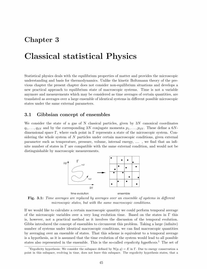
Chapter 3
Classical statistical Physics
Statistical physics deals with the equilibrium properties of matter and provides the microscopicunderstanding and basis for thermodynamics. Unlike the kinetic Boltzmann theory of the pre-vious chapter the present chapter does not consider non-equilibrium situations and develops anew practical approach to equilibrium state of macroscopic systems. Time is not a variableanymore and measurements which may be considered as time averages of certain quantities, aretranslated as averages over a large ensemble of identical systems in different possible microscopicstates under the same external parameters.
3.1 Gibbsian concept of ensembles
We consider the state of a gas of N classical particles, given by 3N canonical coordinatesq1, . . . , q3N and by the corresponding 3N conjugate momenta p1, . . . , p3N . These define a 6N -dimensional space Γ, where each point in Γ represents a state of the microscopic system. Con-sidering the whole system of N particles under certain macroscopic conditions, given externalparameter such as temperature, pressure, volume, internal energy, .... , we find that an infi-nite number of states in Γ are compatible with the same external condition, and would not bedistinguishable by macroscopic measurements.
ensemble
[p]
[q]Γ
t=0
t>0
time evolution
Fig. 3.1: Time averages are replaced by averages over an ensemble of systems in differentmicroscopic states, but with the same macroscopic conditions.
If we would like to calculate a certain macroscopic quantity we could perform temporal averageof the microscopic variables over a very long evolution time. Based on the states in Γ thisis, however, not a practical method as it involves the discussion of the temporal evolution.Gibbs introduced the concept of ensembles to circumvent this problem. Taking a large (infinite)number of systems under identical macroscopic conditions, we can find macroscopic quantitiesby averaging over an ensemble of states. That this scheme is equivalent to a temporal averageis a hypothesis, as it is assumed that the time evolution of the system would lead to all possiblestates also represented in the ensemble. This is the so-called ergodicity hypothesis.1 The set of
1Ergodicity hypothesis: We consider the subspace defined by H(p, q) = E in Γ. Due to energy conservation apoint in this subspace, evolving in time, does not leave this subspace. The ergodicity hypothesis states, that a
45

states for given macroscopic parameters is then represented by a distribution of points in thespace Γ. This distribution is generally continuous for a gas of particles.For the calculation of averages we introduce the density function ρ(p, q) providing the measureof the density of points in Γ-space ((p, q) stands for the whole state (p1, . . . , p3N ; q1, . . . q3N ).Then
ρ(p, q)d3Npd3Nq (3.1)
gives the number of representative points contained in the small volume d3Npd3Nq in Γ, veryanalogous to the distribution function in Boltzmann theory. This can now be used to calculateaverages of any desired quantity which can be expressed in the variable (p, q), A(p, q):
〈A〉 =∫dpdqA(p, q)ρ(p, q)∫
dpdqρ(p, q). (3.2)
We will use from now on the short notation dpdq for d3Npd3Nq where it is not misleading.
3.1.1 Liouville Theorem
The dynamics of the system of N particles shall be described by a Hamiltonian H(p, q) whichyields the equation of motion in the Hamiltonian formulation of classical mechanics.
pi = −∂H∂qi
and qi =∂H∂pi
(i = 1, . . . , 3N) . (3.3)
This equation describes the motion of the points in Γ. If H does not depend on time derivativesof pi and/or qi, then the equations of motion are time reversal invariant. They determine theevolution of any point in Γ uniquely.Now let us consider the points in the Γ space and note that their number does not change intime, as if they form a fluid. Thus, they satisfy the continuity equation
∂ρ
∂t+ ~∇ · (ρ~v) = 0 . (3.4)
where ~v = (p1, . . . , p3N ; q1, . . . , q3N ) and ~∇ = (∂/∂p1, . . . , ∂/∂p3N ; ∂/∂q1, . . . , ∂/∂q3N ). Intro-ducing the generalized substantial derivative we can rewrite this equation as
Dρ
Dt+ ρ~∇ · ~v = 0 . (3.5)
The divergence of the ”velocity” ~v is
~∇ · ~v =3N∑i=1
∂qi∂qi
+∂pi
∂pi
=
3N∑i=1
∂
∂qi
∂H∂pi
− ∂
∂pi
∂H∂qi
︸ ︷︷ ︸
= 0
= 0 (3.6)
This means that the points in Γ space evolve like an incompressible fluid. This property isknown as Liouville’s theorem. We may write this also in the form
0 =Dρ
Dt=∂ρ
∂t+
3N∑i=1
qi∂ρ
∂qi+ pi
∂ρ
∂pi
=∂ρ
∂t+
3N∑i=1
∂H∂pi
∂ρ
∂qi− ∂H∂qi
∂ρ
∂pi
. (3.7)
point on H = E can reach in its temporal evolution every point of this subspace (Boltzmann, 1887). This is notrigorously valid, however. Ehrenfest’s version of this hypothesis (1911) states: The trajectory of a point comesany other point in the same subspace arbitrarily close in the course of time. Of course, it is possible to find(singular) counter examples, for which only a tiny fraction of the subspace is accessed.
46

Using Poisson brackets2 this equation reads,
∂ρ
∂t= H, ρ . (3.9)
3.1.2 Equilibrium system
A satisfactory representation of a system in equilibrium requires for an ensemble that the densityfunction does not depend on time t, i.e. ∂ρ/∂t = 0. From Liouville’s theorem we get thecondition that
0 =3N∑i=1
qi∂ρ
∂qi+ pi
∂ρ
∂pi
= ~v · ~∇ρ = H, ρ . (3.10)
A general way to satisfy this is to take a density function which depends only on quantitiesconserved during the motion, such as energy or particle number. Then the system would evolvewithin a subspace where ρ is constant.We may use this feature of ρ now to consider averages of certain quantities, based on the abovementioned equivalence between the temporal and ensemble averages. Defining the temporalaverage of A(p, q) as
〈A〉 = limT→∞
1T
∫ T
0A(p(t), q(t))dt (3.11)
for any starting point ((p(t = 0), q(t = 0)) in the space Γ and (p(t), q(t)) obeying the equationof motion (3.3). The hypothesis of ergodicity, even in its restricted sense, implies that thisaverage can be taken as an average of an ensemble of an infinite number of different microscopicstates (points in Γ-space). As the evolution of (p, q) conserves the energy, this leads naturallyto consider an ensemble of states of a fixed energy (internal energy). We call such ensemblesmicrocanonical. Although the microcanonical ensemble is not so frequently used in practicethan other ensembles which we will consider later, it is very useful for illustrative purposes. Itdescribes an isolated closed system with no energy exchange with the environment.We postulate that in equilibrium any state of a macroscopic system satisfying the externalconditions appears with equal probability. This is in line with our experience of detailed balancein the previous chapter. In our microcanonical description with fixed energy, number of particlesN and volume V , we postulate
ρ(p, q) =
const. E ≤ H(p, q) ≤ E + δE
0 otherwise(3.12)
where δE is small. The average value of A is then given by (3.2). The validity of this approachis based on the assumption of small mean square fluctuations (standard deviations)
〈A− 〈A〉2〉〈A〉2
1 . (3.13)
Such fluctuations should be suppressed by the order N−1 as we will see below.2The Poisson bracket is defined as
u, v =X
i
∂u
∂qi
∂v
∂pi− ∂u
∂pi
∂v
∂qi
ff= −v, u . (3.8)
47

3.2 Microcanonical ensemble
We consider a macroscopic system of N particles in a volume V which is isolated and closed.The microcanonical ensemble for a given energy E consists of all systems of this kind, whoseenergy lies in the range [E,E + δE]. First we define the phase volume
Φ(E) = ΛN
∫H(p,q)≤E
dpdq , (3.14)
which contains all point in Γ space with energy lower than or equal to E. Moreover, ΛN is arenormalization factor
ΛN =1
N !h3N(3.15)
which compensates for the over-counting of the phase space in the integral by dividing by thenumber equivalent states reached by permutations of the particles, N !. The factor h3N correctsfor the dimension integral to produce a dimensionless Φ(E). Thus, h has the units of action([pq] = Js). While this could be Planck constant h, its magnitude is completely unimportant inclassical statistical physics. From this we obtain the volume of the microcanonical ensemble as
ω(E) = Φ(E + δE)− Φ(E) =dΦ(E)dE
δE . (3.16)
Thus we now can renormalize ρ(p, q) with the condition,
1 =∫dp dq ρ(p, q) =
1ω(E)
∫E≤H(p,q)≤E+δE
dp dq (3.17)
such that
ρ(p, q) =
1
ω(E)E ≤ H(p, q) ≤ E + δE
0 otherwise
. (3.18)
As postulated ρ(p, q) is constant in the energy range [E,E + δE].
3.2.1 Entropy
We use ω(E) to define the entropy
S(E, V,N) = kB lnω(E) (3.19)
This agrees very well with our earlier definition based on the H-function in Eq.(2.20), S =kB lnW where W is the number of configurations for given macroscopic distributions of mi-crostates. Analogously this definition satisfies the general properties of the entropy as we intro-duced them earlier. As earlier we can consider ω(E) or S as a measure of the imprecision of ourknowledge of the state of the system. The more states are available in microcanonical ensemble,the less we know in which state the system is at a given time and the larger is the volume ω andthe entropy.We consider a composite system consisting of two subsystems, 1 and 2,
H(p, q) = H1(p1, q1) +H2(p2, q2) , (3.20)
with (N1, V1) and (N2, V2), resp., for the corresponding particle number and volume. Each ofthe two systems is characterized by ω1(E1) and ω2(E2), respectively. The volume ω(E) of themicrocanonical ensemble is the product of the subsystems under the conditions
E = E1 + E2 , N = N1 +N2 and V = V1 + V2; . (3.21)
48

For simplicity we assume that the volumes and particle numbers of the subsystems may be fixed,while they can exchange energy, such that E1 and e2 can fluctuate. Therefore the volume of themicrocanonical ensemble of the total system for given E reads,
ω(E) =∑
0≤E′≤E
ω1(E′) ω2(E − E′) (3.22)
where we assume for the sum a ”discrete” mesh of equally spaced E′-values of mesh spacing δE( E). We claim that this sum is approximated well by a single value E′
0 giving rise to a sharpmaximum among the summands; (E1 = E′
0 and E2 = E − E′0).
3 The largest term is obtainedby
∂ω1(E′) ω2(E − E′)∂E′
∣∣∣∣E′=E′
0
= 0 (3.25)
such that
0 =
1ω1(E′)
∂ω1(E′)∂E′ +
1ω2(E − E′)
∂ω2(E − E′)∂E′
E′=E′
0
=∂ lnω1(E1)
∂E1
∣∣∣∣E1=E′
0
− ∂ lnω2(E2)∂E2
∣∣∣∣E2=E−E′
0
.
(3.26)
From this we obtain with E1 = E′0 and E2 = E − E′
0
∂S1(E1)∂E1
∣∣∣∣E1=E1
=∂S2(E2)∂E2
∣∣∣∣E2=E2
(3.27)
which can be considered as the equilibrium condition. Note that this is equivalent to the state-ment that the equilibrium state corresponds to the macrostate with the largest number of mi-croscopic realizations.
Identifying E as the internal energy U we define the temperature
∂S
∂U=
1T
⇒ 1T1
=1T2
, (3.28)
leading to T as an equilibrium state variable. We have ignored the other variables V,N whichwe will consider later.Let us assume that there is some impediment which forces the two subsystems to specific vari-ables such that each subsystem independently is at equilibrium, but not the total system. Forexample, a big vessel of gas may be separated by a wall into two subvessels. Then we find forthe corresponding ω of the combined system,
ω(E, V,N) = ω1(E1, V1, N1)ω2(E2, V2, N2) with
E = E1 + E2
V = V1 + V2
N = N1 +N2
(3.29)
such that the entropy
S(E, V,N) = S1(E1, V1, N1) + S2(E2, V2, N2) ≤ S(E, V,N) , (3.30)3Note that lnωi ∝ Ni and Ei ∝ Ni (i = 1, 2) as both quantities are extensive. We then find quickly the
following bounds:
ω1(E′0)ω2(E − E′
0) ≤ ω(E) ≤ E
δEω1(E
′0)ω2(E − E′
0) . (3.23)
Note that E/δE is the number of summands. Thus, we obtain for the entropy
kB lnω1(E′0)ω2(E − E′
0) ≤ S(E) ≤ kB lnω1(E′0)ω2(E − E′
0) + kB lnE
δE. (3.24)
It is important to see that the last term only scales with system size as lnN (keeping δE fixed), while the firstterm scales with N . Therefore in the very large-N limit the last term is irrelevant. Which proves that S(E) isgiven by the maximal term in the sum (3.22).
49

i.e. the entropy is concave. This means also the equilibrium is obtained by the maximal entropy,which is a consequence of the second law of thermodynamics. In terms of the volume of themicrocanonical volume ω the equilibrium state assumes among all volumes the maximal one,the most likely one in terms of probability.
3.2.2 Relation to thermodynamics
We have with (3.19) a definition of the entropy analogous to the expression of H in (2.115,2.116)which for the variables E(= U), V andN is a thermodynamic potential and allows us to calculatea variety of state variables and relations,
dS =(∂S
∂E
)V,N
dE +(∂S
∂V
)E,N
dV +(∂S
∂N
)E,V
dN =1TdE +
p
TdV − µ
TdN . (3.31)
This allows also to calculate the thermodynamic equation of state,
p = T
(∂S
∂V
)E,N
(3.32)
and to determine other thermodynamic potentials. The caloric equation of state is obtainedfrom (
∂S
∂U
)V,N
=1T. (3.33)
using U = E is the internal energy. The derivative with respect to N yields finally the chemicalpotential
µ = −T(∂S
∂N
)E,V
, (3.34)
the energy to add a particle to the system.
3.3 Discussion of ideal systems
3.3.1 Classical ideal gas
We consider a classical gas of N independent mono-atomic particles in the fixed volume V ,which is closed and isolated. The Hamiltonian is simply given by
H(p, q) = H(p) =N∑
i=1
~p2i
2m. (3.35)
Hence we obtain the volume
Φ(E) = ΛN
∫H(p)≤E
dpdq = ΛNVN
∫H(p)≤E
dp (3.36)
This p-integral corresponds to the volume of a sphere of Radius R in 3N -dimensional space.4
The integral is straightforward,
Φ(E) = ΛNVNC3N (2mE)3N/2 with Cn =
πn/2
Γ(
n2 + 1
) (3.39)
4Volume of sphere in ν-dimensional space: V(R) = CRν . The volume enclosed in a thin shell of width δR atthe Radius R is given by
vshell = V(R)− V(R− δR) = CRν
»1−
„1− δR
R
«ν–(3.37)
with δR R. In the limit ν very large, νδR R, we find
vshell ≈ V(R) . (3.38)
Thus, the main part of the volume in the sphere is concentrated at the outermost shell.
50

where C3N is the proper prefactor for the volume of an 3N -dimensional sphere.5 This leads to
ω(E) =∂Φ(E)∂E
δE = ΛNC3NVN 3N
22m (2mE)3N/2−1 δE . (3.42)
Remarkably, for very large N (∼ 1023) we find that the following definitions for the entropy areidentical up to terms of order lnN and constants:
Sω = kB lnω(E, V,N) and SΦ = kB lnΦ(E, V,N) (3.43)
leading to
Sω = kB ln(ΛNVNC3N ) + kB
(3N2− 1)
ln(2mE) + kB ln(
3N2
2mδE)
= kB ln(ΛNVNC3N ) + kB
3N2
ln(2mE) +O(lnN) = SΦ +O(lnN) .
(3.44)
Since we can drop terms of order lnN for the extensive entropy, we will continue, for convenience,using SΦ instead of Sω,
S(E, V,N) = NkB ln
V
(2mπEh2
)3/2− 3N
2kB ln
3N2
+3N2kB −NkB lnN +NkB (3.45)
where we used Stirling’s formula
lnn! ≈ n lnn− n+12
ln(2πn) for n→∞ , (3.46)
and neglected all terms of order lnN . We then rewrite
S(E, V,N) = NkB ln
V
N
(4πmE3Nh2
)3/2
+52NkB . (3.47)
This equation may now be solved for E so that we obtain the internal energy as a thermodynamicpotential
U(S, V,N) = E =3N5/3h
4πmV 2/3exp
2S
3NkB− 1. (3.48)
The thermodynamic quantities are obtained by derivation: the temperature
T =(∂U
∂S
)V,N
=2U
3NkB⇒ U =
32NkBT , (3.49)
the pressure
p = −(∂U
∂V
)S,N
=23U
V=NkBT
V⇒ pV = NkBT , (3.50)
and the chemical potential
µ =(∂U
∂N
)S,N
=U
N
(53− 2
3S
NkB
)= −kBT ln
V
N
(2πmkBT
h2
)3/2. (3.51)
Through further derivatives it is possible to obtain various response functions, as previouslydiscussed in chapter 1. The ideal gas is readily described by means of the microcanonicalensemble.
5Prefactor Cn: Use the n-dimensional Gaussian integral in Cartesian coordinates
I =
Z +∞
−∞dx1 · · ·
Z +∞
−∞dxne
−(x21+···+x2
n) =
„Z +∞
−∞dxe−x2
«n
= πn/2 . (3.40)
The same integral in spherical coordinates is given by
I = nCn
Z ∞
0
drrn−1e−r2=n
2Cn
Z ∞
0
dt tn2 −1e−t =
n
2CnΓ
“n2
”= CnΓ
“n2
+ 1”
(3.41)
such that we obtain Cn given in (3.39). Note, Γ(n+ 1) = n! for n ≥ 0 as an integer.
51

3.3.2 Ideal paramagnet
Consider a system of N independent magnetic moments. Each moment has only two directions+m and −m (Ising moments: two-state units). Now apply a magnetic field H in which thesemoments are either parallel or antiparallel, as described by the Hamiltonian
H(mi) = −N∑
i=1
Hmi with mi = ±m , (3.52)
so that the two states have different energy. In contrast to the gas, these degrees of freedom arediscrete. We determine now the volume ω(E) in the space of (m1, . . . ,mN ). For this purposewe define the magnetization of the systems as
M =∑
i
mi = nm ⇒ H(mi) = −HM = −Hnm . (3.53)
Fixed energy means a fixed number n, i.e. 12(N + n) moments are positively and 1
2(N − n)negatively oriented (H > 0). The number of configuration with fixed n are then given by
ω(M) =N ![
12(N + n)
]![
12(N − n)
]!. (3.54)
We can define the probability for the magnetization M by dividing ω(M) with the total numberof configurations, 2N . Let us now evaluate lnω using Stirling’s formula,
lnω(M) = N lnN −N +12
ln(2πN)− N
2
(1 +
n
N
)lnN
2
(1 +
n
N
)−N
2
(1− n
N
)lnN
2
(1− n
N
)+N
2
(1 +
n
N
)+N
2
(1− n
N
)−1
2lnπ2N2
(1− n2
N2
).
(3.55)
Neglecting terms of order lnN we obtain
lnω(M) = −N2
(1 +
n
N
)ln(1 +
n
N
)+(1− n
N
)ln(1− n
N
)+N ln 2 , (3.56)
which can be used to express the entropy,
S(E) = kB lnω(E)
= NkB ln 2− NkB
2
(1 +
E
HmN
)ln(
1 +E
HmN
)+(
1− E
HmN
)ln(
1− E
HmN
)(3.57)
with E = −nHm and introducing H as external parameter (state variable). From this we obtain
1T
=(∂S
∂E
)H
= − kB
2Hmln(HmN + E
HmN − E
)
⇒ E(T ) = U(T ) = −NHm tanh(Hm
kBT
).
(3.58)
Using the following differential we determine the magnetization
dS =1TdU +
M
TdH − µ
TdN
⇒ M = T
(∂S
∂H
)E
=kBTE
2H2mln(HmN + E
HmN − E
)= −E
H= Nm tanh
(Hm
kBT
).
(3.59)
52

This is the thermodynamic equation of state of this system. In the limit Hm kBT we findthe so-called Curie-type behavior of independent magnetic moments,
M = NHm2
kBT(3.60)
and in the opposite limit the magnetization tends to saturate,
M = Nm(1− 2e−2Hm/kBT
). (3.61)
The heat capacity for constant external field H is given by(∂S
∂T
)H
=(∂S
∂E
)H
(∂E
∂T
)H
=CH
T(3.62)
Substituting E in Eq.(3.57) by Eq.(3.58) we obtain
CH = T
(∂S
∂T
)H
=N(Hm)2
kBT 2
1
cosh2(
HmkBT
) . (3.63)
A further response function is the differential magnetic susceptibility at finite magnetic field H,
χ′(T ) =(∂M
∂H
)=Nm2
kBTcosh−2
(Hm
kBT
)(3.64)
which corresponds to the ”linear response”. For the limit of H → 0 we obtain,
χ(T ) =Nm2
kBT, (3.65)
corresponding to the famous Curie-susceptibility of independent magnetic moments.
χ’
k T / Hm
NC
B
Fig. 3.2: heat capacity and differential susceptibility (magnitude in arbitrary units): Bothquantities show a maximum around mH ∼ kBT . At low temperature both are exponentiallysuppressed ∼ T−αe−2Hm/kBT , which is indicating a freezing of the degrees of freedom, i.e. at
T = 0 all magnetic moments are pointing in the same direction.
53

3.4 Canonical ensemble
We change to a macroscopic system for which we control the temperature by connecting it to avery large heat reservoir. The system together with the reservoir forms a closed system of giventotal energy. Therefore we consider two subsystems, system 1 describing our system and system2 being the heat reservoir:
H(p, q) = H1(p1, q1) +H2(p2, q2) . (3.66)
The heat reservoir is much larger than system 1: N2 N1, such that energy transfer betweenthe two subsystems would be too small to change the temperature of the reservoir. Withinthe microcanonical scheme we determine the phase space of the combined system in the energyrange
E ≤ E1 + E2 ≤ E + δE . (3.67)
E , S , T
11
2 2
E , S , T
Fig. 3.3: The two systems 1 and 2 are coupled thermally. System 2 acts as a huge reservoirfixing the temperature of the system 1 which we want to investigate.
Therefore the volume of the microcanonical ensemble of the total system is
ω(E) =∑
0≤E1≤E
ω1(E1)ω2(E − E1) (3.68)
Analogous to our previous discussion in section 3.2.1, there is one value E1 = E′0 (E2 = E−E′
0)which provides the by far dominant contribution. In addition here E2 E1 is valid. Thecorresponding volumes in Γ-space are ω1(E1) and ω2(E2) and ω(E) ≈ ω1(E1)ω2(E − E1). Dueto this simple product form we can determine the density function ρ1(p1, q1) of the system 1, byconsidering the mean value of A(p, q) in system one.
〈A〉1 =
∫1 dp1dq1A(p1, q1)
∫2 dp2dq2ρ(p, q)∫
1 dp1dq1∫2 dp2dq2ρ(p, q)
=
∫1 dp1dq1A(p1, q1)ρ1(p1, q1)∫
1 dp1dq1ρ1(p1, q1). (3.69)
Taking into account that ρ(p, q) is constant in the range E ≤ H1(p1, q1) +H2(p2, q2) ≤ E + δEwe obtain
〈A〉1 =
∫1 dp1dq1A(p1, q1)ω2(E −H1(p1, q1))∫
1 dp1dq1ω2(E −H1(p1, q1))(3.70)
Using the assumption that E2 ≈ E E1 we may expand ω2(E −H1(p1, q1)) in H1(p1, q1)):
kB lnω2(E −H1(p1, q1)) = S2(E −H1(p1, q1)) = S2(E)−H1(p1, q1)∂S2(E2)∂E2
∣∣∣∣E2=E
+ · · ·
= S2(E)− H1(p1, q1)T
+ · · ·(3.71)
54

from which we derive
ω2(E −H1(p1, q1)) = eS2(E)/kBe−H1(p1,q1)/kBT . (3.72)
Here T is the temperature of both systems which are in equilibrium.Within the canoncial ensemble, taking the temperature T as a given parameter, we write
generally for the density function, the probability to find the system of N particles in themicrostate (p, q),
ρ(p, q) =1Ze−H(p,q)/kBT . (3.73)
where we introduced the partition function Z
Z = ΛN
∫dp dqe−βH(p,q) with β =
1kBT
, (3.74)
which, up to prefactors, corresponds to the volume of the ensemble of system 1, called canonicalensemble, again renormalized by ΛN .6
3.4.1 Thermodynamics
The connection to thermodynamics is given by the relation
Z = e−βF (T,V,N) , (3.75)
where F (T, V,N) is the Helmholtz free energy, a thermodynamical potential. Note, F is anextensive quantity, because obviously scaling the system by a factor λ would yield Zλ. Moreover,
F = U − TS (3.76)
with
U = 〈H〉 and S = −(∂F
∂T
)V,N
. (3.77)
This can be proven using the equation,
1 = ΛN
∫dp dqeβ(F−H) , (3.78)
which through differentiation with respect to β on both sides gives,
0 = ΛN
∫dp dqeβ(F−H)
F + β
(∂F
∂β
)V,N
−H
⇒ F (T, V,N)− U(T, V,N)− T
(∂F
∂T
)V,N
= 0 .
(3.79)
Using this formulation for the free energy we obtain for the pressure
p = −(∂F
∂V
)T,N
. (3.80)
which in the case of a gas leads to the thermodynamic equation of state.The internal energy is obtained easily from the partition function in the following way:
U(T, V,N) = 〈H〉 =ΛN
Z
∫dp dq He−βH = − 1
Z
∂Z
∂β= − ∂
∂βlnZ . (3.81)
This is the caloric equation of state.6Note that there is, rigorously speaking, the constraintH1(p1, q1) < E. However, in the approximation ignoring
this constraint is good enough, as the main contribution is from the valid range.
55

3.4.2 Equipartition law
We now consider a set of special average values which will lead us to the so-called equipartitionlaw, the equal distribution of energy on equivalent degrees of freedom. We examine the meanvalue, ⟨
qµ∂H∂qν
⟩=
ΛN
Z
∫dp dqqµ
∂H∂qν
e−βH = −ΛN
Zβ
∫dp dqqµ
∂
∂qνe−βH
= −ΛN
Zβ
∫ ′dp d′q qµe
−βH︸ ︷︷ ︸= 0
+ΛNδµν
Zβ
∫dpdqe−βH = δµνkBT ,
(3.82)
where we used integration by parts leading to the boundary terms in the qj-coordinate (expressedby∫ ′d′q...), which we assume to vanish. Analogously we find for the momentum⟨
pµ∂H∂pν
⟩= δµνkBT . (3.83)
If the Hamiltonian is separable into a p-dependent kinetic energy and a q-dependent potentialenergy part and, moreover, if the following scaling behavior is valid
H(p, q) = Ekin(p) + V (q) with Ekin(λp) = λ2Ekin(p) and V (λq) = λαV (q) (3.84)
then we can use the above relations and find for mono-atomic particles
〈Ekin〉 =3N2kBT and 〈V 〉 =
3NαkBT . (3.85)
The total energy is given by the sum of the two contributions.
Diatomic molecules: An interesting aspect appears in the case of multi-atomic molecules, as suchthey have internal degrees of freedom and a binding potential. We consider here a system ofN atoms forming diatomic molecules. Molecules form due to a binding two-particle interaction:V (q) =
∑i<j Vij(q) with Vij(q) = v(|~qi − ~qj |). A good approximation for the binding potential
is the Lenard-Jones potential composed of an attractive and a ”hard-core” repulsive part,
v(r) = 4ε
(r
r
)12
−(r
r
)6, (3.86)
with ε as the potential depth and r0 = 21/6r as the minimal point (Fig. 3.4). Around theminimum the potential can be approximated up to a constant by a harmonic potential,
v(r) ≈ A(r − r0)2 with A = 36ε/21/3r2 . (3.87)
V
−6
r −12
harmonic
r
r
Fig. 3.4: Lenard-Jones potential.
56

The Hamiltonian is given by
H(p, q) =N∑
i=1
~pi2
2m+∑i<j
v(|~qi − ~qj |) (3.88)
which leads for the kinetic energy part through the equipartition law, Ekin = 3NkBT/2. Forthe potential energy part we find,
kBT =⟨qµi
∂H∂qµ
i
⟩, (3.89)
which does not lead to a simple form for the potential energy contribution to the internal energy.For low temperatures (ε kBT ) we may use Eq.(3.87) and calculate the partition function fora single molecule (the kinetic energy part factorizes out and is omitted here),
Zv =∫d3re−βv(r) = 4π
∫ ∞
0dr r2e−βA(r−r0)2 ≈ 4πr20
∫ +∞
−∞dy e−βAy2
= 4πr20
√π
Aβ, (3.90)
which then yields,
〈v〉 = − ∂
∂βlnZv =
kBT
2. (3.91)
This is the potential energy contribution of a one-dimensional harmonic oscillator (radial part).Together with the kinetic energy part we obtain
U = 〈Ekin〉+ 〈V 〉 =3N2kBT +
N
2〈v〉 ≈ 7N
4kBT =
N
2
52kBT + kBT︸︷︷︸
harmonic oscillator
. (3.92)
This result is interesting in the following sense. The heat capacity of the dissociated moleculesat high temperature is lower than the one of the diatomic molecule, although there are moreindependent particles at high temperature:
CV
N=
1N
(∂U
∂T
)V,N
=
3kB
2kBT ε
7kB
4kBT ε
. (3.93)
This result is independent of the sharpness of the harmonic potential. However, if we turnto the limit of the rigid molecular bond, i.e. no harmonic potential (or infinitely sharp), thenthe situation changes. The motion of the two atoms is constraint by the rigidity condition:(~pi − ~pj) · (~qi − ~qj) = 0. Then the internal energy is given by
U =5N4kBT ⇒ CV
N=
5kB
4. (3.94)
The change to this value is singular within classical statistical mechanics. Only quantum me-chanics is able to describe the ”freezing out” of the vibrational degree of freedom. In fact withinthe quantum mechanical description we find even a further lowering when the rotational degreesof freedom freeze out such that eventually U = 3NkBT/4. Further temperature lowering thenrequires to consider the system as a quantum liquid of Bosons or Fermions.
57

3.4.3 Fluctuation of the energy and the equivalence of microcanonial andcanonical ensembles
The internal energy is given as the average of the Hamiltonian U = 〈H〉. Therefore the followingrelation holds:
ΛN
∫dp dq [U −H] eβ(F−H) = 0 . (3.95)
Taking the derivative of this equation with respect to β we obtain
0 =∂U
∂β+ ΛN
∫dp dq (U −H)
[F − T
∂F
∂T−H
]eβ(F−H) =
∂U
∂β+ 〈(U −H)2〉 . (3.96)
This leads to the relation for the fluctuations of the energy around its average value U ,
〈H2〉 − 〈H〉2 = 〈(U −H)2〉 = −∂U∂β
= kBT2∂U
∂T= kBT
2CV , (3.97)
as we had seen in section 2.2.3. Because CV is an extensive quantity and therefore proportionalto N , it follows that
〈H2〉 − 〈H〉2
〈H〉2∝ 1N
(3.98)
which is a sign of the equivalence of microcanonical and canonical ensembles. In the thermo-dynamic limit N → ∞, the fluctuations of the energy vanish compared to the energy itself.Therefore the internal energy as U = 〈H〉 = E is a well defined quantity in the canonicalensemble as well as it was in the microcanonical ensemble.
We now consider the partition function
Z = ΛN
∫dp dq e−βH(p,q) =
∫ ∞
0dE ω(E)e−βE =
∫ ∞
0dE e−βE+ln ω(E) =
∫ ∞
0dE eβ(TS(E)−E)
(3.99)where the entropy S(E) is defined according to the microcanonical ensemble. The maximum ofthe integrand at E = E0 is defined by the condition
T∂S
∂E
∣∣∣∣E=E0
= 1 and∂2S
∂E2
∣∣∣∣E=E0
< 0 . (3.100)
Note that∂2S
∂E2
∣∣∣∣E=E0
=∂
∂E
1T
∣∣∣∣E=E0
= − 1T 2
∂T
∂E
∣∣∣∣E=E0
= − 1T 2CV
< 0 . (3.101)
If we now expand the exponent in the integrand, we obtain
TS(E)− E = TS(E0)− E0 −1
2TCV(E − E0)2 + · · · (3.102)
such that with U = E0,
Z ≈ eβ(TS−U)
∫ ∞
0dE e−(E−U)2/2kBT 2CV = eβ(TS−U)
√2πkBT 2CV
⇒ F ≈ U − TS − 12kBT ln
2πkBT
2CV
= U − TS +O(lnN) .
(3.103)
Since the free energy is extensive, the term of order lnN is in the large-N limit irrelevant.
58

3.4.4 Ideal gas in canonical ensemble
Consider a gas of N particles without external potential and mutual interactions described bythe Hamiltonian
H(p) =N∑
i=1
~pi2
2m. (3.104)
The partition function is given by
Z = ΛN
N∏i=1
∫d3pi d
3qi e−~pi
2/2mkBT = ΛN
∫d3p d3q e−~p 2/2mkBT
N
= ΛNVN 2πmkBT3N/2 .
(3.105)
From this we obtain the free energy and the internal energy using Stirling’s formula,
F (T, V,N) = −kBT lnZ = −NkBT ln
V
N
(2πmkBT
h2
)3/2−NkBT ,
U(T, V,N) = − ∂
∂βlnZ =
3N2kBT (caloric equation of state) .
(3.106)
The entropy is given by
S(T, V,N) = −(∂F
∂T
)V,N
= NkB ln
V
N
(2πmkBT
h2
)3/2
+5N2kB (3.107)
and the pressure by
p = −(∂F
∂V
)T,N
=NkBT
V(3.108)
which corresponds to the thermodynamic equation of state. Finally the chemical potential isobtained as
µ =(∂F
∂N
)T,V
= −kBT ln
V
N
(2πmkBT
h2
)3/2. (3.109)
An important aspect for the ideal system is the fact that the partition function has a productform because each particle is described independently. In this way it leads to an extensive freeenergy and internal energy.
3.4.5 Ideal paramagnet
As a next example we consider again an ideal paramagnet. Unlike the example discussed in themicrocanonical ensemble we use here a magnetic moment ~m which can point in any direction(full rotational symmetry) and is represented as a vector of fixed length m. The magneticmoment can be represented by two angles of orientation in spherical coordinates,
~m(φ, θ) = m(sin θ cosφ, sin θ sinφ, cos θ) (3.110)
building the phase space of each moment with the volume element dΩ = dφdθ sin θ = dφd cos θ.The externally applied magnetic field couples in the usual Zeeman form,
H(~mi) = −N∑
i=1
~mi · ~H = −N∑
i=1
mH cos θi (3.111)
59

where θi denotes the angle between magnetic field and moment (magnetic field defines z-axis).It is easy to calculate now the partition function
Z =N∏
i=1
∫dΩi e
βmH cos θi =
2π∫ +1
−1dx e−βmHx
N
=
4πmHβ
sinh(βmH)N
= ZNm . (3.112)
This again shows the product form. The thermodynamics is again obtained via the free energyand the internal energy,
F (T,H,N) = −kBT lnZ = NkBT ln(βmH)−NkBT ln4π sinh(βmH)
U(T,H,N) = NkBT −NmH coth(βmH)(3.113)
From this we obtain according to Eq.(3.63),
CH(T,H,N) =(∂U
∂T
)H
= NkB −N(mH)2
kBT 2
1sinh2(mH/kBT )
. (3.114)
where we use the magnetization M derived below. This yields the limiting behaviors
CH =
NkB
3
(mH
kBT
)2
kBT mH
NkB
(1− 4
(mH
kBT
)2
e−2mH/kBT
)kBT mH
(3.115)
Analogous to our previous ideal paramagnet, the magnetic field enters as a characteristic energyscale separating two regimes of thermodynamics.
0 2 4 6 8 10kBT / mH
0
0.2
0.4
0.6
0.8
1
< m
Z >
/ m
0 2 4 6 8 10mH / kBT
0
0.2
0.4
0.6
0.8
1
< m
z >
/ m
Fig.3.5: Mean magnetization per moment: left panel, as a function of temperature and fixedmagnetic field, with full saturation at T = 0; right panel, as a function of magnetic field and
fixed temperature, with full saturation at mH kBT .
The magnetization can be calculated as
〈~m〉 =1Zm
∫dΩ ~m(φ, θ)e−β ~m· ~H (3.116)
with Eq.(3.110) leading to 〈mx〉 = 〈my〉 = 0 ( ~H ‖ z) and
〈mz〉 = m coth(mH
kBT
)− kBT
H= mL(mH/kBT ) (3.117)
60

which corresponds to
〈~m〉 = − 1N
(∂F
∂ ~H
)T,N
. (3.118)
The function L(x) = coth(x) − 1/x is also called Langevin function in literature. The secondderivative with respect to ~H yields the magnetic susceptibility as a response function (in thelimit of ~H → 0 it is the linear response)7
χzz(T ) = −(∂2F
∂H2z
)T,N
=Nm2
kBT
[(kBT
mH
)2
− 1sinh2(mH/kBT )
]
=
N
m2
3kBTkBT mH
Nm2
kBT
(kBT
mH
)2
− 4e−2mH/kBT
kBT mH
(3.120)
It is interesting to study the fluctuations of the magnetization,
〈m2z〉 − 〈mz〉2 = m2
[(kBT
mH
)2
− 1sinh2(mH/kBT )
]=kBT
Nχzz . (3.121)
Note that here the zero-temperature limit of the heat capacity does not vanish, but is NkB andcorresponds to the contribution of the potential energy of a two-dimensional harmonic oscillator(the fluctuating magnetic moment nearly aligned with magnetic field feels a harmonic potential).Analogous to the fluctuations of the energy discussed above we find that the fluctuations of themagnetization are connected with a response function, the susceptibility.8 This is a simplifiedversion of the so-called fluctuation-dissipation theorem which will encounter later again.
3.4.6 More advanced example - classical spin chain
We now go beyond the ideal paramagnetic system by considering a chain of spins (magneticmoments) ~si which interact with each other via nearest-neighbor coupling in the followingway:
H(~si) = J
N∑i=1
~si · ~si+1 (3.125)
where J is the coupling strength. For J < 0 the spins tend to align parallel (ferromagnetic) andfor J > 0 they tend to be antiparallel, alternating (antiferromagnetic). This chain is open andoccupied regularly by N + 1 spins (N bonds).
7Generally we define
N〈mν〉 = −„∂F
∂Hν
«T,N
and χνν′ = −„
∂2F
∂Hν∂Hν′
«T,N
. (3.119)
8Generally we find the relation for the fluctuations of the magnetization ~M =P
i ~mi from the followingargument:
0 =
ZdΩ1 · · · dΩN (〈 ~M〉 − ~M)eβ(F−H) (3.122)
taking the derivative with respect to the field leads to
0 =∂〈Mz〉∂H
− βZdΩ1 · · · dΩN (〈Mz〉 −Mz)
2eβ(F−H) = χzz − β〈(〈Mz〉 −Mz)2〉 . (3.123)
This yields the convenient relation,
χzz =1
kBT
˘〈M2
z 〉 − 〈Mz〉2¯. (3.124)
61

J > 0
J
ferromagnetic antiferromagnetic
J < 0
Fig.3.6: Spin chain: Coupling J between spins of arbitrary orientation. J < 0: ferromagneticalignment preferred; J > 0: antiferromagnetic alignment preferred.
Interestingly the topology of the coupling allows to calculate the partition function exactly. Weconsider the spins as vectors of fixed length S and write the partition function as
Z =∫dΩ1 · · · dΩN+1 e
−βJP
i ~si·~si+1 , (3.126)
which decays into product form, if we consider the reference polar axis (”z-axis”) for the spin~si given by the direction of the spin ~si+1 (θi is defined as angle between ~si and ~si+1). Thereforewe may write
Z =N∏
i=1
∫e−βJ~si·~si+1dΩi
∫dΩN+1 =
N∏i=1
∫e−βJS2 cos θidΩi
∫dΩN+1
= 4π
2π∫ +1
−1dxe−βJS2x
N
= 4π
4πsinh(βJS2)βJS2
N
(3.127)
which looks similar to the expression obtained for the ideal paramagnet. We may actuallyconsider each spin being subject to the Zeeman field induced via the coupling by the neighboringspins (mean field idea). It is interesting to see that Z does not depend on the sign of J . Thus,the thermodynamics is the same for a ferromagnetic and an antiferromagnetic chain.Easily we can determine the free and the internal energy,
F (T,N) = NkBT ln(βJS2)−NkBT lnsinh(βJS2)
−NkBT ln 4π
U(T,N) = NkBT −NJS2 coth(βJS2)(3.128)
which leads to the heat capacity
C = NkB
1−
(βJS2
sinh(βJS2)
)2
(3.129)
with a similar form as for the ideal paramagnet.
Correlation function: Now we turn to a new aspect which did not encounter in the ideal param-agnet. The question of the mutual influence of spins is not meaningful in the ideal paramagnet,since the spins are completely independent. Moreover, there was no topology which would tellus the ”distance” between two spins. The same is true for the positions of particles in an idealgas. For our spin chain, however, the question of how the orientation of spin ~si influences the
62

orientation of spin ~si+l makes sense, since we have a clear topology and coupling among thespins. We define the correlation function
Γl = 〈~si · ~si+l〉 = 3〈szi s
zi+l〉
=3Z
∫dΩ1 · · · dΩN+1S
2 cos Θi cos Θi+le−βJS2
Pi cos θi .
(3.130)
where Θi is the angle of spin i with respect to the general z-axis (e.g. along the chain). Wecan perform all integrations for the spin ~sj with j < i and j > i+ l which decay into the sameproduct form as discussed above. The remaining integrals are now
Γl = 3S2
(βJS2
4π sinh(βJS2)
)l ∫dΩi cos Θie
−βJS2 cos θi
×∫dΩi+1e
−βJS2 cos θi+1 · · ·∫dΩi+l cos Θi+l
(3.131)
Taking again the spin si+1 as a reference of the spin si we find the relation9
cos Θi = cos Θi+1 cos θi + sinΘi+1 sin θi cosφi . (3.134)
Inserting this we notice that the averages 〈cos θi〉 6= 0 and 〈sin θi cosφi〉 = 0. Thus
Γl = 3S2
(βJS2
4π sinh(βJS2)
)l ∫dΩi cos θie
−βJS2 cos θi
×∫dΩi+1 cos Θi+1e
−βJS2 cos θi+1 · · ·∫dΩi+l cos Θi+l
= Γl−1βJS2
4π sinh(βJS2)
∫dΩi cos θie
−βJS2 cos θi = Γl−1u(βJS2)
(3.135)
withu(x) =
1x− cothx . (3.136)
If we take into account that Γl=0 = S2 we find
Γl = S2[u(βJS2)
]l = S2e−l/ξ(−sign(J))l with ξ−1 = − ln|u(βJS2)| . (3.137)
Note that 0 < u < 1 for all finite temperatures and couplings. The correlation function decaysexponentially for all finite temperature with a correlation length ξ:
ξ(T ) =
[ln(kBT/|J |S2)]−1 kBT |J |S2
|J |S2
kBTkBT |J |S2
(3.138)
9Consider ~s1 and ~s2 and take y′ ⊥ z, ~s2 with |y′| = |z| = 1:
~s1 = ~s2 cos θ1 + (y′ × ~s2) sin θ1 cosφ1 + y′S sin θ1 sinφ1 (3.132)
and multiply by z:z · ~s1| z
=S cos Θ1
= cos θ1 z · ~s2| z =S cos Θ2
+~y′ · (~s2 × z)| z =y′S sin Θ2
sin θ1 cosφ1 . (3.133)
63

For large temperature the correlation length shrinks rather slowly to zero and in the zero-temperature limit it diverges indicating an infinitely extending correlation. Indeed we find forT = 0 that u→ 1 such that
Γl(T = 0) = S2(−signJ)l (3.139)
for all l. This means that the spins order either ferromagnetically for J < 0 or antiferromagnet-ically for J > 0 at T = 0. However, for any finite temperature Γl → 0 for l→∞.Finally we want to study the susceptibility assuming a coupling to the magnetic field of the form
H′ = H− g
N+1∑i=1
~si · ~H , (3.140)
χ
ferromagnetic
antiferromagnetic
a)
1/
b)
Fig.3.7: Thermodynamic properties of spin chain: a) heat capacity: saturates at lowtemperature to NkB like the potential energy of a two-dimensional harmonic oscillator; b)
Susceptibility plotted inversely: ferromagnetic case show divergence at T = 0 andantiferromagnetic case approaches non-monotonically a finite value at T = 0. Extrapolations
from high-temperature region cut horizontal axis at positive (ferromagnetic) and negative(antiferromagnetic) axis, indicating effective energy scales for the corresponding correlations.
since it is impossible to use the above scheme to calculate the partition function with a finitemagnetic field coupling to the magnetic moments. Therefore, we will use the relation derivedearlier (3.124) based on the fluctuations of the magnetization, which does not require the knowl-edge of the partition function at finite fields.
χzz =g2
kBT
N+1∑i=1
N+1∑j=1
〈sz
i szj 〉 − 〈sz
i 〉〈szj 〉. (3.141)
The second term on the right hand side vanishes, since 〈szi 〉 = 0 for all i, as can be easily shown.
For the first term we can use our result for the correlation function. In the limit of very largeN we obtain
χzz =g2
3kBT
N+1∑i=1
N+1∑j=1
Γ|i−j| ≈g2
3kBT
N∑i=1
(Γl=0 + 2S2
∞∑l=1
ul
)
=g2N
3kBTS2
(1 +
2u1− u
)=g2S2N
3kBT
1 + u(βJS2)1− u(βJS2)
.
(3.142)
Here we use that for large systems (N → ∞) the corrections due to boundary contributions isvery small. This susceptibility at high temperature (kBT JS2) follows the Curie behavior
χzz =g2S2N
3kBT(3.143)
64

irrespective of the sign of J . For the antiferromagnetic coupling χzz goes through a maximum atkBTmax ≈ 0.238JS2 to a finite zero-temperature value. On the other hand, for the ferromagneticcase χzz diverges at low temperatures
χzz = Ng2S2
32|J |S2
(kBT )2, (3.144)
more strongly than the Curie 1/T behavior.Let us now also look at the first lowest order correction in the high-temperature limit,
1χzz
≈ 3kBT
g2S2N
(1 +
2JS2
3kBT
)=
3kB
g2S2N(T −ΘW ) ⇒ χzz =
C
T −ΘW(3.145)
where ΘW = −2JS2/3kB defines the so-called Weiss temperature. Thus the extrapolation fromthe high-temperature limit of 1/χzz allows from the intersection on the temperature axis todetermine ΘW and consequently the sign and magnitude of the J (see dashed lines in Fig. 3.6).
3.5 Grand canonical ensemble
We consider now a new situation by allowing beside the heat exchange also the exchange ofmatter of our system with a very large reservoir. Thus we take the system 1 with N1 particlesin a volume V1 coupled to the reservoir 2 with N2 particles in the volume V2 with
N1 N2 and V1 V2 , (3.146)
and N = N1 +N2 and V = V1 + V2 fixed. The Hamiltonian can be decomposed into two parts
H(p, q,N) = H(p1, q1, N1) +H(p2, q2, N2) (3.147)
such that the corresponding partition function for given temperature (everything is coupled toan even larger heat reservoir) is given by
ZN (V, T ) =1
h3NN !
∫dp dq e−βH(p,q,N) . (3.148)
The factor 1/N ! takes into account that all possible commutation of the particles give the samestates (distinguishable classical particles). Now we segregate into the subsystems fixing thevolumes and particle numbers (N2 = N −N1),
ZN =1
h3NN !
N∑N1=0
N !N1!N2!
∫dp1 dp2
∫V1
dq1
∫V2
dq2e−βH(p1,q1,N1)+H(p2,q2,N2)
=N∑
N1=0
1h3N1N1!
∫V1
dp1 dq1 e−βH(p1,q1,N1) 1
h3N2N2!
∫V2
dp2 dq2 e−βH(p2,q2,N2)
(3.149)
Note that the distribution of the particles into the two subsystems is not fixed yielding thecombinatorial factor of N !/N1!N2! (number of configurations with fixed N1 and N2 by permutingthe particles in each subsystem). From this we define the probability ρ(p1, q1, N1) that we canfind N1 particles in the volume V1 at the space coordinates (p1, q1),
ρ(p1, q1, N1) =e−βH(p1,q1,N1)
ZNN1!h3N2N2!
∫V2
dp2 dq2 e−βH(p2,q2,N2) (3.150)
which is renormalized asN∑
N1=0
1h3N1
∫V1
dp1dq1ρ(p1, q1, N1) = 1 (3.151)
65

We may write
ρ(p1, q1, N1) =ZN2
ZN
1N1!
e−βH(p1,q1,N1) , (3.152)
where we now use the relation
ZN2(V2, T )ZN (V, T )
= e−βF (T,V−V1,N−N1)−F (T,V,N) (3.153)
with
F (T, V − V1, N −N1)−F (T, V,N) ≈ −(∂F
∂V
)T,N
V1−(∂F
∂N
)T,V
N1 = −µN1 + pV1 . (3.154)
Thus we definez = eβµ (3.155)
which we call fugacity. Thus within the grand canonical ensemble we write for the densityfunction
ρ(p, q,N) =zN
N !e−βpV +H(p,q,N) . (3.156)
µ is the chemical potential as introduced earlier. We now introduce the grand partition function
Z(T, V, z) =∞∑
N=0
zNZN (V, T ) , (3.157)
which incorporates all important information of a system of fixed volume, temperature andchemical potential.
3.5.1 Relation to thermodynamics
We use now (3.156) and integrate both sides
1 = e−βpV∞∑
N=0
zN
N !
∫dp dq
h3Ne−βH(p,q,N) = e−βpV Z(T, V, z) (3.158)
which leads toΩ(T, V, µ) = −pV = −kBT lnZ(T, V, z) , (3.159)
the grand potential:dΩ = −SdT − pdV −Ndµ . (3.160)
The average value of N is then given by
〈N〉 = −(∂Ω∂µ
)T,V
= kBT∂
∂µlnZ = z
∂
∂zlnZ =
1Z
∞∑N=0
NzNZN . (3.161)
It is also convenient to derive again the internal energy
U = − ∂
∂βlnZ ⇒ CV =
(∂U
∂T
)V,µ
. (3.162)
We consider now the fluctuations of the particle number. The following relation holds
〈N2〉 − 〈N〉2 = z∂
∂zz∂
∂zlnZ = z
∂
∂z
1Z∑N
NzNZN =1Z∑N
N2zNZN −
1Z∑N
NzNZN
2
(3.163)
66

from which we derive
〈N2〉 − 〈N〉2 = −kBT∂2
∂µ2Ω(T, V, µ) = kBT
∂〈N〉∂µ
. (3.164)
We now relate the right hand side with the isothermal compressibility. Introducing the specificvolume v = V/N we consider µ = µ(v, T ) (note that µ is not extensive). Moreover we use theGibbs-Duhem relation (1.72),
dµ = v dp− S
NdT ⇒
(∂µ
∂v
)T
= v
(∂p
∂v
)T
. (3.165)
Since v depends on both V and N , the following derivatives are useful(∂
∂v
)V,T
=(∂N
∂v
)V,T
(∂
∂N
)V,T
= −N2
V
(∂
∂N
)V,T
,
(∂
∂v
)N,T
=(∂V
∂v
)N,T
(∂
∂V
)N,T
= N
(∂
∂V
)N,T
.
(3.166)
From (3.165) then conclude
− N2
V
(∂µ
∂N
)V,T
= V
(∂p
∂V
)N,T
⇒ 1N
(∂N
∂µ
)V,T
= − 1vV
(∂V
∂p
)N,T
=κT
v. (3.167)
Consequently the fluctuations of the particle number is connected with the response function,κT , the isothermal compressibility:
κT =v
〈N〉kBT
〈N2〉 − 〈N〉2
. (3.168)
3.5.2 Ideal gas
For the ideal gas, it is easy to calculated the grand partition function (here for simplicity we seth = 1),
Z(T, V, z) =∞∑
N=0
zNZN (T, V ) =∞∑
N=0
zN
N !V N (2πmkBT )3N/2 = exp
zV (2πmkBT )3/2
(3.169)
We can also derive the probability PN of finding the system with N particles. The average valueis given by
〈N〉 = z∂
∂zzV (2πmkBT )3/2 = zV (2πmkBT )3/2 ⇒ Z = e〈N〉 (3.170)
From this we conclude that the distribution function for the number of particles is given by
PN = e−〈N〉 〈N〉N
N !≈ 1√
2π〈N〉e−(N−〈N〉)2/2〈N〉 (3.171)
which is strongly peaked at N = 〈N〉 1.10 The fluctuations are given by
〈N2〉 − 〈N〉2 = z∂〈N〉∂z
= 〈N〉 ⇒ κT =v
kBT=
1p
(3.172)
The grand potential is given by
Ω(T, V, µ) = −kBTeβµV (2πmkBT )3/2 = −kBT 〈N〉 = −pV (3.173)
The chemical potential is obtained solving Eq.(3.170) for µ as
µ = kBT ln
(〈N〉(2πmkBT )−3/2
V
). (3.174)
10Note that for µ > 0 it pays the energy µ to add a particle to the system. Therefore as T goes to 0 the averageparticle number 〈N〉 increases (diverges). Oppositely, 〈N〉 decreases for T → 0, if µ < 0 and energy has to bepaid to add a particle.
67

3.5.3 Chemical potential in an external field
In order to get a better understanding of the role of the chemical potential, we now consider anideal gas in the gravitational field, i.e. the particles are subject to the potential φ(h) = mgh.We introduce a reference chemical potential µ0 as a constant. Then we write for the chemicalpotential,
µ = µ0 +mgh+ kBT lnn(2πmkBT )−3/2
(3.175)
where we define n = 〈N〉/V as the local number density of particles. In equilibrium the tem-perature and the chemical potential shall be constant. We may determine µ by the conditionthat at h = 0 the density is n = n0,
µ(T ) = µ0 + kBT lnn0(2πmkBT )−3/2
⇒ mgh = kBT ln
(n0
n
)(3.176)
We can now solve this equation for n = n(h):
n(h) = n0e−βmgh . (3.177)
and with the (local) equation of state
p(h) = n(h)kBT = p0e−βmgh (3.178)
This is the famous barometer formula.
3.5.4 Paramagnetic ideal gas
As a further example, we consider an ideal gas of particles with a magnetic moment which onlycan point in two directions, parallel or antiparallel to an applied magnetic field. Thus, theHamiltonian is given by
H(p, q,H) =∑
i
~pi2
2m−∑
i
miH , (3.179)
where mi = ±m. Having now an ideal gas of two types of particles, moment parallel (+)and antiparallel (−) to H, we treat this problem in the grand canonical ensemble language.We introduce the corresponding particle numbers N+ and N−. The grand canonical partitionfunction is easily calculated as
Z =∑N
1N !
N++N−=N∑N+,N−
N !N+! N−!
V az+e
βHmN+
V az−e
−βHmN−
=∑N+
1N+!
V az+e
βHmN+ ∑
N−
1N−!
V az−e
−βHmN−
= expz+e
βmHV a
expz−e
−βmHV a
(3.180)
with a = (2πmkBT )3/2. The average numbers of up and down magnetic moments are then
N± = z±∂
∂z±lnZ = z±e
±βmHV a (3.181)
From this we derive the chemical potential, z± = eβµ± ,
µ± = kBT ln(n±a
)∓ mH , (3.182)
68

where n± = N±/V . In equilibrium µ+ = µ− = µ otherwise the system would shift the distribu-tion of moments, N+ ↔ N−. This leads to the ratio
N+
N−=n+
n−= e2βmH . (3.183)
The partial pressures defined by
p± =N±kBT
V⇒ p = p+ + p− (3.184)
add up to the total pressure. The number of particles and the magnetization are given by
N = N+ +N− = 2V aeβµ cosh(βmH) and M = m(N+ −N−) = 2mV aeβµ sinh(βmH)(3.185)
Under the condition that there is an external reservoir of particles at the chemical potential µ,we can define the magnetization per particle in the system,
M
N= m tanh(βmH) , (3.186)
as we had obtained earlier for the ideal paramagnet.
69

Chapter 4
Quantum Statistical Physics
Quantum statistical physics opens the door to new phenomena and also provides an under-standing of the third law of thermodynamics, which we had found to be often violated withinclassical statistical physics. Moreover, we will find that for ideal quantum gases the concept ofindistinguishable particles leads to the classification of particles into two categories: Bosons andFermions.
4.1 Basis of quantum statistics
Every state of a quantum mechanical system can be described by a superposition of stationarystates |ψn〉 of the Hamiltonian H, which form a complete orthonormalized basis,
|Ψ〉 =∑
n
cn|ψn〉 (4.1)
where the complex coefficients cn represent the wavefunction whose time dependence is deter-mined by the Hamiltonian H. For the stationary states the following holds:
H|ψn〉 = εn|ψn〉 with 〈ψn|ψn′〉 = δnn′ (4.2)
The renormalization of the state |Ψ〉 requires,
1 = 〈Ψ|Ψ〉 =∑n,n′
c∗ncn′〈ψn|ψn′〉 =∑
n
|cn|2 . (4.3)
The square modulus |cn|2 denotes the probability to find the state |ψn〉 in |Ψ〉.Observable quantities are represented by Hermitian operators A, and their expectation value is
〈Ψ|A|Ψ〉 =∑n,n′
c∗ncn′〈ψn|A|ψn′〉 . (4.4)
This expectation value is generally time dependent: cn = cn(t).Considering now a measurement of a macroscopic observable, which corresponds to an average(indicated here by over-bar) over a time much longer than the microscopic time scales (timebetween collisions, inverse energy spacing, etc.).
〈Ψ|A|Ψ〉 =∑n,n′
c∗ncn′〈ψn|A|ψn′〉 (4.5)
Let us now restrict to eigenstates in a certain narrow energy range: E ≤ εn ≤ E + ∆ (micro-canonical point of view). The quantum statistical physics is based on two key postulates:
70

• Equal probability:
c∗ncn =
r , E ≤ εn ≤ E + ∆ ,
0 , otherwise .(4.6)
where r is a real constant.
• Random phase: if n 6= n′ thenc∗ncn′ = 0 , (4.7)
i.e. the phase of the wavefunction is a random variable. Such a behavior requires an atleast weak coupling to the environment in order to randomize the phases.
As a consequence averaged expectation values are given by
〈Ψ|A|Ψ〉 =∑
n
|cn|2〈ψn|A|ψn〉 (4.8)
which corresponds to considering the state |Ψ〉 as an incoherent superposition of the eigenstates(pure versus mixed state). We may consider the drop out of interference terms as an effect ofaveraging over a long time whereby the phases depend on time. Alternatively, we average overan ensemble of many different states with different phases.
4.2 Density matrix
Mixed states or incoherent superpositions of states are conveniently described by density matricesρ. We define first the density matrix as an operator through its matrix elements
〈ψn|ρ|ψn′〉 = ρnn′ = |cn|2δnn′ (4.9)
In the basis of stationary states the density matrix is diagonal. Therefore we may formally writethe density matrix in spectral form as
ρ =∑
n
|cn|2|ψn〉〈ψn| . (4.10)
We may also express the average value of A as a trace of the form,
〈A〉 =∑
n〈ψn|Aρ|ψn〉∑n〈ψn|ρ|ψn〉
=tr(Aρ)trρ
(4.11)
Note that the final expression is independent of the basis |ψn〉, as known from standard linearalgebra. The cyclic permutation of matrices (operators) does not change the trace: tr(ABC) =tr(BCA). Thus the basis transformation U yields A′ = UAU−1, such that
tr(A′) = tr(UAU−1) = tr(AU−1U) = tr(A) . (4.12)
In this sense the density matrix is a convenient tool to perform ensemble averages as it containsbasis-free informations. In order to describe equilibrium properties ρ should not depend on timet and commutes with the Hamiltonian:
i~∂ρ
∂t= [H, ρ] = 0 . (4.13)
It is obvious that the density matrix defined in (4.10) commutes with H. Compare this withLiouville’s theorem of classical mechanics.
71

4.3 Ensembles in quantum statistics
We now formulate the quantum statistical physics in terms of the three types of ensembles whichwe introduced for the classical statistical physics.
4.3.1 Microcanonical ensemble
The microcanonical ensemble is suitable for closed systems which do not exchange energy andparticles with the environment. We take the density matrix in its diagonal form ρnn′ = δnn′ |cn|2.In this ensemble we consider an incoherent state which consist of the equally distributed set ofstates within a certain narrow energy range between E and E + δE. Thus,
|cn|2 =
1 E ≤ εn ≤ E + δE
0 otherwise(4.14)
The energies εn are the eigenenergies of the stationary states |ψn〉 for the Hamiltonian H.Formally we then write the density matrix as
ρ =∑
E≤εn≤E+δE
|ψn〉〈ψn| with trρ =∑
n
ρnn = ω(E) (4.15)
Here ω(E) is the number of quantum states |ψn〉 with energy in the given energy range. Anal-ogous to the classical case we use now ω(E) to define the entropy
S(E, V ) = kB lnω(E) . (4.16)
From this we may derive the thermodynamics. Note that ω(E) is connected with the density ofstates dΦ(E)/dE of the quantum system.
Φ(E) =∑
n
Θ(E − εn) ⇒ ω(E) =dΦ(E)dE
δE . (4.17)
with Θ(x) as the step function
Θ(x) =
1 x > 00 x ≤ 0
. (4.18)
4.3.2 Canonical ensemble
For a system which is in thermal equilibrium with a reservoir of given temperature T we usethe canoncial ensemble formulation. Analogous to the classical statistical physics we define thedensity matrix here as
ρ(p, q) = e−βH(p,q) → ρnn′ = δnn′e−βεn . (4.19)
and we define the partition function as
Z =∑
n
e−βεn = trρ = e−βF (T,V,N) (4.20)
where F is the Helmholtz free energy. The density matrix can be written as an operator,
ρ =∑
n
|ψn〉e−βεn〈ψn| = e−βH∑
n
|ψn〉〈ψn|︸ ︷︷ ︸=1
= e−βH . (4.21)
Thus the partition function can also be expressed as
Z = tre−βH (4.22)
72

and average values of observables are given by
〈A〉 =tr(Ae−βH)tre−βH =
1Ztr(Ae−βH
). (4.23)
The connection to thermodynamics is given via the Helmholtz free energy,
F (T, V,N) = −kBT lnZ . (4.24)
4.3.3 Grandcanonical ensemble
Now we connect the system in addition to the heat reservoir also to the particle reservoir ofgiven chemical potential µ. In the same spirit as for the canonical ensemble we use the analogyto the classical systems. The density matrix now reads,
ρ = e−β(H−µN) (4.25)
with N the particle number operator and the grandcanonical partition function is then
Z = tre−β(H−µN) =∑N
zNZN (4.26)
with z = eβµ as the fugacity, leading to the grand potential
Ω(T, V, µ) = −kBT lnZ . (4.27)
4.3.4 Ideal gas in grandcanonical ensemble
A gas of independent particles in quantum mechanics has the additional key feature that indis-tinguishable particles are categorized in Fermions (particles with half-integer spins) and Bosons(particles with integer spins). The former follow the Pauli principle: we cannot find two Fermionsin the same quantum state. For Bosons no such restriction exists. A many-particle state ofBosons (Fermions) is described by wavefunction which is completely symmetric (antisymmetric)under the pair-wise exchange of particle variables.1 The free particles in quantum mechanicsare represented by plane waves
ψ~p(~r) = 〈~r|ψ~p〉 =1√Vei~p·~r/~ with ε~p =
~p 2
2m. (4.32)
1Many-body wavefunction of N identical particles: We consider the single-particle states |ψi〉 with ψi(~r) =〈~r|ψi〉. For Bosons the wave function is given by
Ψ(B)1,2,...,N (~r1, ~r2, . . . , ~rN ) =
s Qj Nj !
N !
XP∈SN
ψP (1)(~r1)ψP (2)(~r2) · · ·ψP (N)(~rN ) (4.28)
where SN is the group of all permutations P of N elements and Nj is the multiplicity of the different single-particlestates among the N particles. This wave function is symmetric under exchange of two particles,
Ψ(B)1,2,...,N (. . . , ~ri, . . . , ~rj , . . .) = Ψ
(B)1,2,...,N (. . . , ~rj , . . . , ~ri, . . .) . (4.29)
For Fermions the wave function is antisymmetric,
Ψ(F )1,2,...,N (~r1, ~r2, . . . , ~rN ) =
1√N !
XP∈SN
sign(P )ψP (1)(~r1)ψP (2)(~r2) · · ·ψP (N)(~rN ) (4.30)
where the exchange of two particles leads to a sign change through sign(P ),
Ψ(f)1,2,...,N (. . . , ~ri, . . . , ~rj , . . .) = −Ψ
(f)1,2,...,N (. . . , ~rj , . . . , ~ri, . . .) . (4.31)
Note that this many-body state is described by an unique wavefunction where all permutations particles areincluded. For the classical states this is not case and all combinations have to be counted.
73

The grand partition function for a gas of such particles is given by
Z =∑n~p
gn~pe−β(E−µN)n~p , (4.33)
withE =
∑~p
ε~pn~p and N =∑
~p
n~p . (4.34)
Here n~p is the number of particles per state, the occupation number, whereby the sum∑
n~pruns over all allowed configurations of occupations. The factor gn~p is given by
gn~p =
1 indistinguishable particles (Fermions and Bosons) ,
∏~p
1n~p!
classical particles (Boltzmann) .(4.35)
Each many-particle quantum state for indistinguishable particles includes all permutationsthrough the total symmetrization (Bosons) or antisymmetrization (Fermions) of the wavefunc-tion. For Fermions we find that for each state |ψ~p〉 the occupation number is n~p = 0, 1 and forBosons n~p = 0, 1, 2, . . .. Thus, calculating the partition function we obtain for Fermions/Bosons,
Z =∑
n~p1,n~p2
,...
[ze−βε~p1
n~p1ze−βε~p2
n~p2 · · ·]
=∏~p
∑n~p
(ze−βε~p
)n~p
=
∏~p
(1 + ze−βε~p
)Fermions
∏~p
11− ze−βε~p
Bosons
(4.36)
with z = eβµ as the fugacity.2
From the partition function we arrive at the equation of state
pV
kBT= −βΩ(T, V, µ) =
∑~p
ln(1 + ze−βε~p
)Fermions ,
−∑
~p
ln(1− ze−βε~p
)Bosons ,
(4.38)
and the particle number
N = z∂
∂zlnZ =
∑~p
1eβε~pz−1 + 1
Fermions ,
∑~p
1eβε~pz−1 − 1
Bosons .
(4.39)
2 Classical particles: The partition function is given by
Z =X
n~p1,n~p2
,...
»1
n~p1 !
nze−βε~p1
on~p1 1
n~p2 !
nze−βε~p2
on~p2 · · ·–
=∞X
N=0
zN 1
N !
8<:X~p
e−βε~p
9=;N
=∞X
N=0
zNZ(class)N ,
(4.37)which corresponds to the usual partition function of independent classical particles within the grandcanonicalensemble.
74

These equations can be used to determine the chemical potential, if we fix N . The occupationnumber of a state is also easily obtained,
〈n~p〉 =1Z
∞∑N=0
zN
P~p′ n~p′=N∑n~p′
n~pe−β
P~p′ ε~p′n~p′ = −kBT
∂
∂ε~plnZ
=
1
z−1eβε~p + 1Fermions ,
1z−1eβε~p − 1
Bosons .
(4.40)
These correspond to the Fermi-Dirac and the Bose-Einstein distributions, respectively.Eventually we compare the grand potential and the internal energy. Using (4.38) we obtain
Ω = ∓kBT∑
~p
ln(1± ze−βε~p
)= ∓kBT
∫dε g(ε) ln
(1± ze−βε
)
= ∓V kBT1
4π2
(2m~2
)3/2 ∫ ∞
0dε ε1/2 ln(1± ze−βε)
= −23V
14π2
(2m~2
)3/2 ∫ ∞
0dε
ε3/2
z−1eβε ± 1,
(4.41)
where the plus (minus) sign stands for the Fermions (Bosons). For the second equality weperformed an integration by parts. We have also introduced the density of states
g(ε) =∑
~p
δ(ε− ε~p) = V1
4π2
(2m~2
)3/2
ε1/2 , (4.42)
for the energy integration. Now consider the internal energy
U =∑
~p
〈n~p〉ε~p = V1
4π2
(2m~2
)3/2 ∫ ∞
0dε
ε3/2
z−1eβε ± 1. (4.43)
Thus from Ω = −pV we obtain the general relation
U =32pV . (4.44)
Note that we did not so far include the spin s of the particles in our considerations. This givesan additional factor 2s+ 1 to Ω and U .
4.4 Properties of Fermi gas
We consider now Fermions of spin s, i.e. there are 2s+1 different species. The equation of stateand the equation for the particle number of the Fermi gas are given by
p
kBT=
4πh3
(2s+ 1)∫ ∞
0dp p2 ln
(1 + ze−βε~p
),
1v
=N
V=
4πh3
(2s+ 1)∫ ∞
0dp p2 1
z−1eβε~p + 1.
(4.45)
75

where we used the relation∑
~p = Vh3
∫d3p. We rewrite these equations introducing special
functions of z,p
kBT=
2s+ 1λ3
f5/2(z)
1v
=2s+ 1λ3
f3/2(z)
(4.46)
where λ = h/√
2πmkBT is the thermal wavelength. These functions are defined as3
f5/2(z) =4√π
∫ ∞
0dx x2 ln(1 + ze−x2
) = −∞∑l=1
(−1)l zl
l5/2
f3/2(z) = z∂
∂zf5/2(z) = −
∞∑l=1
(−1)l zl
l3/2
(4.48)
For the following it will also be important to consider the asymptotic behavior of these functions.For z 1 we may use the expansion just given. For z 1 we find4
f5/2(z) ≈8
15√π
(ln z)5/2
[1 +
5π2
8(ln z)2+ · · ·
]
f3/2(z) =4
3√π
(ln z)3/2
[1 +
π2
8(ln z)2+ · · ·
] (4.52)
4.4.1 High-temperature and low-density limit
Low density (high temperature) implies λ3 v = V/N and z = eβµ 1 . We can use now(4.46)
λ3
v= (2s+1)
z − z2
23/2+ · · ·
⇒ z =
λ3
v
12s+ 1
+1
23/2(2s+ 1)2
(λ3
v
)2
+ · · · . (4.53)
3Expansion of f5/2(z):
4√π
Z ∞
0
dx x2 ln(1 + ze−x2) = − 4√
π
Z ∞
0
dx
∞Xl=1
x2(−1)l zle−lx2
l= −
∞Xl=1
(−1)l zl
l5/2. (4.47)
4Derivation of the large-z-expansion: Use ν = µ/kBT = ln z and rewrite
f5/2(z) =2√π
Z ∞
0
dy y1/2 ln(1 + eν−y) =8
15√π
Z ∞
−ν
dy′(y′ + ν)5/2 ey′
(1 + ey′)2, (4.49)
where the second equation is obtained by twice integrating by parts. More over we extend the lower integrationboundary to −∞, at the expense of a small error of order e−ν = 1/z. We now expand (y′ + ν)5/2 assuming νlarge and find
f5/2(z) =8
15√π
Z +∞
−∞dy′
»ν5/2 +
5
2ν3/2y′ +
15
8ν1/2y′
2+ · · ·
–ey′
(1 + ey′)2
=8
15√π
»I0ν
5/2 +5
2I1ν
3/2 +15
8I2ν
1/2 + · · ·– (4.50)
where
In =
Z +∞
−∞dy
yney
(1 + ey)2⇒ I0 = 1, I1 = 0, I2 =
π2
3, . . . . (4.51)
Note that all In = 0 for n odd. It is easy to obtain f3/2(z) by taking the derivative.
76

This allows us to replace z in the equation of state 5,
p
kBT≈ 2s+ 1
λ3
z − z2
25/2
≈ N
V
1 +
N
25/2(2s+ 1)λ3
V
(4.55)
The second term represents the first quantum correction to the classical limit of the ideal gas.This allows us also to calculate the isothermal compressibility,
κT = − 1V
(∂V
∂p
)T,N
=V
NkBT
11 + λ3N
23/2V (2s+1)
(4.56)
The quantum correction decreases the compressibility, as a consequence of Pauli’s exclusionprinciple, i.e. Fermions avoid each other. The occupation numbers is approximatively given by
〈n~p〉 ≈λ3
v
12s+ 1
e−βε~p =Nh3
V (2πmkBT )3/2e−βε~p (4.57)
corresponding to the Maxwell-Boltzmann distribution. With the general relation (4.44) weobtain immediately the internal energy and the heat capacity
U ≈ 32NkBT
1 +
Nλ3
25/2(2s+ 1)V
and CV =
32NkB
1− Nλ3
27/2(2s+ 1)V
, (4.58)
including the first quantum corrections.
4.4.2 Low-temperature and high-density limit: degenerate Fermi gas
At low temperature we reach the ”quantum limit” λ3 v = V/N , which implies large fugacityz. First we consider the zero-temperature situation. The occupation numbers follow a stepfunction
〈n~p〉 = Θ(µ− ε~p) =
1 , ε~p < µ ,
0 , ε~p > µ .. (4.59)
The Fermions occupy states within a sphere in momentum space, the Fermi sphere. The particledensity n is
n =N
V=
2s+ 1h3
∫d3p〈n~p〉 =
2s+ 1h3
4π3p3
F =(2s+ 1)k3
F
6π2(4.60)
where pF is the Fermi momentum (ε~pF= µ(T = 0) = εF ), isotropic, and kF = pF /~ is the Fermi
wavevector. The groundstate energy is
U0 =2s+ 1h3
V
∫d3pε~p〈n~p〉 =
35NεF (4.61)
where εF denotes the Fermi energy. The zero-point pressure is obtained through (4.38),
p0 =23U
V=
25N
VεF . (4.62)
In contrast to the classical ideal gas, a Fermi gas has finite zero-point pressure which is againa consequence of the Pauli principle and is responsible for the stability of metals, neutron starsetc.
5Note that the lowest order expansion reproduces the chemical potential of the classical ideal gas, as given inEq.(3.51) and (3.109):
z = eβµ ≈ N
Vλ3 ⇒ µ = −kBT ln
(V
N
„2πmkBT
h2
«3/2). (4.54)
77

pz
py
px
pF
Fig.4.1: Fermi sphere of occupied single particle states. Fermi radius pF .
Next we turn to finite temperatures for which the occupation number broadens the step at pF .We use now (4.52, 4.60) to obtain the relation(
εFkBT
)3/2
=34
√πλ3
2s+ 1N
V=(
µ
kBT
)3/2
+π2
8
(µ
kBT
)−1/2
+ · · · , (4.63)
which at constant density n = N/V can be solved for the chemical potential,
µ(T ) = εF
(1− π2
12
(kBT
εF
)2
+ · · ·
), (4.64)
and in very much the same way we obtain for the pressure,
p(T ) = p0
(1 +
5π2
12
(kBT
εF
)2
+ · · ·
). (4.65)
Again we derive the internal energy from the relation (4.38)
U =32pV =
35NεF
(1 +
5π2
12
(kBT
εF
)2
+ · · ·
), (4.66)
which also leads to the heat capacity for fixed N
CN = kBNπ2
2kBT
εF+ · · · . (4.67)
This is the famous linear temperature dependence of the heat capacity, which can be observedwell for the electrons in simple metals. Obviously now the third law of thermodynamics issatisfied: CN
T→0→ 0. Also the entropy goes to zero linearly in T .
4.4.3 Spin-1/2 Fermions in a magnetic field
We consider now the magnetic response of spin s = 1/2 Fermions in a magnetic field (idealparamagnetic gas). The Hamiltonian has to be extended by a Zeeman term. Taking the fieldalong the z-axis this reads,
HZ = −gµB
N∑i=1
sziH (4.68)
with g = 2 as gyromagnetic ratio and µB the Bohr magneton. This can be absorbed into aspin-dependent fugacity,
zs = eβµ+sβµBH , (4.69)
78

with s = + or −, such that the density of Fermions is given by
n =N
V=
1v
=1λ3
f3/2(z+) + f3/2(z−)
= n+ + n− (4.70)
and the magnetization
m =M
V= µB(n+ − n−) =
µB
λ3
f3/2(z+)− f3/2(z−)
. (4.71)
Let us now calculation the spin susceptibility for zero magnetic field, given by
χ =∂m
∂H
∣∣∣∣H=0
=µ2
B
λ3kBT2z∂f3/2(z)∂z
∣∣∣∣H=0
=2µ2
B
λ3kBTf1/2(z) (4.72)
with z = eβµ. We may now again consider limiting cases.
High-temperature limit: We replace z 1 in Eq.(4.72) using Eq.(4.53) with n = 1/v and find
χ =µ2
Bn
kBT
1− λ3n
25/2
. (4.73)
The first term is the result for particles with spin and has a Curie like behavior (compare withSect.3.5.4) and the second term is the first quantum correction reducing the susceptibility.
Low-temperature limit: Taking only the lowest order for z 1 we obtain,
χ =µ2
B
λ3kBT
4√π
(ln z)1/2 =µ2
B
λ3kBT
4√π
(εFkBT
)1/2
= µ2B
3n2εF
. (4.74)
This is the famous Pauli spin susceptibility for a Fermi gas, which temperature independent.
4.5 Bose gas
There are two situations for Bosons: (1) a system with well-defined particle number, e.g. bosonicatoms, 4He, ... ; (2) Bosons which results as modes of harmonic oscillators (no fixed particlenumber), e.g. photons, phonons, magnons, etc..
4.5.1 Bosonic atoms
We consider Bosons without spin (S = 0) for which 4He is a good example. Analogous to theFermions we introduce functions of z to express the equation of state and the particle number,
p
kBT=
1λ3g5/2(z) =
1λ3
∞∑l=1
zl
l5/2
1v
=N
V=
1λ3g3/2(z) =
1λ3
∞∑l=1
zl
l3/2.
(4.75)
For small z both functions grow linearly from zero and g3/2(z) has a divergent derivative forz → 1. We concentrate on the range 0 < z ≤ 1, such that µ(T ) ≤ 0. For z = 1 we obtain
g3/2(1) =∑
l
1l3/2
= ζ(3/2) ≈ 2.612 and g5/2(1) =∑
l
1l5/2
= ζ(5/2) ≈ 1.342 (4.76)
where ζ(x) is Riemann’s ζ-function.
79

g5/2
g3/2
Fig.4.2: Functions g3/2(z) and g5/2(z).
4.5.2 High-temperature and low-density limit
It is easy to see that like the Fermions the Bosons behave in this limit as a classical ideal gas.An intriguing aspect occurs, however, in the quantum corrections. For the pressure we find
p(T ) =N
VkBT
1− N
25/2
λ3
V+ · · ·
. (4.77)
The quantum correction reduces the classical ideal gas pressure and yields the compressibility
κT = − 1V
(∂V
∂p
)T,N
=V
NkBT
11− λ3N
23/2V
(4.78)
In contrast to the Fermions where the quantum nature of the particles diminishes the compress-ibility, here the compressibility is enhanced. Actually, in this approximation the compressibilityeven diverges, if
23/2 =N
Vλ3 (4.79)
i.e. at low enough temperature or high enough density. We will now see that this indeed indicatesan instability of the Bose gas.
4.5.3 Low-temperature and high-density limit: Bose-Einstein condensation
Let us now consider equation (4.75) carefully. The function g3/2(z) is monotonically increasingwith z. If T is lowered, λ ∝ T−1/2 increases, such that z has to increase too in order to satisfy(4.75). Therefore µ approaches the singular point at 0 (z = 1). The critical point is determinedby
g3/2(1) = ζ(3/2) =N
Vλ3 ⇒
Tc =
h2
2πkBm[ζ(3/2)V/N ]2/3,
Vc =N
ζ(3/2)h3
(2πmkBT )3/2.
(4.80)
This defines a critical temperature Tc and critical volume Vc below which a new state of the Bosegas occurs. Note that this equation is qualitatively very similar to (4.79) and even quantitativelynot so far (ζ(3/2) ≈ 2.612 ↔ 23/2 ≈ 2.85) . The question arises what happens for T < Tc orV < Vc. Actually the problem occurring in (4.75) and (4.80) arises in the step
N =∑
~p
1eβ(ε~p−µ) − 1
→ V
h3
∫d3p
1eβ(ε~p−µ) − 1
. (4.81)
80

The integral does not count the occupation of the state ~p = 0, because the momentum distribu-tion function entering the integral,
ρ(p) =p2
eβ(ε~p−µ) − 1⇒ ρ(0) = 0 . (4.82)
This is fine as long as the occupation of the ~p = 0-state (single-particle groundstate) is vanish-ingly small compared to N . However, for T < Tc (V < Vc) the occupation becomes macroscopic,〈n~p=0〉/N > 0 and we cannot neglect this contribution in the calculation of N . Thus the correctdensity is
N
V=
1λ3g3/2(z) + n0(T ) = nn(T ) + n0(T ) (4.83)
with n0(T ) denoting the density of Bosons in the single-particle groundstate (~p = 0). Theseparticles form a condensate, the Bose-Einstein condensate. What happens at Tc is a phasetransition. We encounter here a ”two-fluid” system for which the total particle density splitinto a condensed fraction n0 and a normal fraction nn. From (4.83) we find the temperaturedependence of n0,
n0(T ) =N
V
[1−
(T
Tc
)3/2]. (4.84)
1
nnn0
n0
p TTc
n
Fig.4.3: Occupation: Left panel: A macroscopic fraction of particle occupy the momentump = 0-state for T < Tc. Right panel: Temperature dependence of the condensate fraction.
Next we also determine the equation of state,
p =
kBT
λ3g5/2(z) , V > Vc
kBT
λ3g5/2(1) , V < Vc
(4.85)
We now consider the compressibility for V > Vc . For this purpose we first determine
∂V
∂z= −Nλ3
g′3/2(z)
g3/2(z)2, (4.86)
and consider
∂p
∂V=kBT
λ3g′5/2(z)
∂z
∂V⇒ κT =
Nλ6
V kBTg3/2(z)2g′3/2(z)
g′5/2(z). (4.87)
where we use the notation g′n(z) = dgn(z)/dz. As anticipated earlier the compressibility divergesat the transition V → Vc (or T → Tc), since the derivative g′3/2(z) → ∞ for z → 1. In thecondensed phase the pressure is independent of V as is obvious from (4.85). Therefore thecondensed phase is infinitely compressible, i.e. it does not resist to compression.
81

Some further thermodynamic quantities can be derived. First we consider the entropy S fromthe grand canonical potential
S(T, V, µ) = −(∂Ω∂T
)V,µ
=(∂pV
∂T
)V,µ
=
NkB
(5v2λ3
g5/2(z)− ln z), T > Tc ,
NkB52g5/2(1)g3/2(1)
(T
Tc
)3/2
, T < Tc .
(4.88)
where we used (4.75).6 For the heat capacity at fixed particle number N we find from theinternal energy U = 3
2pV ,
CV =(∂U
∂T
)V,N
=
NkB
(15v4λ3
g5/2(z)−94g3/2(z)g1/2(z)
), T > Tc ,
NkB154g5/2(1)g3/2(1)
(T
Tc
)3/2
, T < Tc .
(4.92)
T
V
NkB
Tc
3/2
C
Fig.4.4: heat capacity: CV has a cusp at the transition and vanishes as T 3/2 towardszero-temperature. In the high-temperature limit Cv approaches 3NkB/2 which corresponds to
the equipartition law of a mono-atomic gas.
In accordance with the third law of thermodynamics both the entropy and the heat capacity goto zero in the zero-temperature limit. The entropy for T < Tc can be viewed as
S
N= s
(T
Tc
)3/2
=nn(T )n
s with s =52kB
g5/2(1)g3/2(1)
(4.93)
where s is the entropy per normal particle (specific entropy), i.e. a non-vanishing contributionto the entropy is only provided by the normal fraction (two-fluid model). The heat capacity hasa cusp at T = Tc.
6Calculation of the temperature derivatives: (1) Fixed chemical potential:
∂
∂T
V kBT
λ3g5/2(z) =
5V kB
λ3g5/2(z) +
V kBT
λ3
g3/2(z)
z
∂z
∂T| z = −kB
V
λ3g3/2(z)βµ = −NkB ln z
(4.89)
where we used ∂∂zg5/2 = g3/2/z.
(2) Fixed particle number: we use
g3/2(z) =N
Vλ3 ⇒
dg3/2
dT=g1/2(z)
z
dz
dT= −3
2
N
V
λ3
T(4.90)
which leads to the relationdg5/2
dT=g3/2(z)
z
dz
dT= −9
4
g3/2(z)
g1/2(z)
Nλ3
V. (4.91)
This leads to the expression for the heat capacity.
82
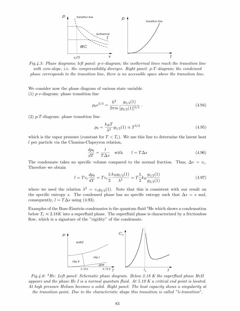
BEC
cv
p
T
isothermal
p
T
transition line
transition line
v (T)
Fig.4.5: Phase diagrams; left panel: p-v-diagram; the isothermal lines reach the transition linewith zero-slope, i.e. the compressibility diverges. Right panel: p-T -diagram; the condensed
phase corresponds to the transition line, there is no accessible space above the transition line.
We consider now the phase diagram of various state variable.(1) p-v-diagram: phase transition line
p0v5/3 =
h2
2πmg5/2(1)
[g3/2(1)]5/3. (4.94)
(2) p-T -diagram: phase transition line
p0 =kBT
λ3g5/2(1) ∝ T 5/2 (4.95)
which is the vapor pressure (constant for T < Tc). We use this line to determine the latent heatl per particle via the Clausius-Clapeyron relation,
dp0
dT=
l
T∆vwith l = T∆s (4.96)
The condensate takes no specific volume compared to the normal fraction. Thus, ∆v = vc.Therefore we obtain
l = Tvcdp0
dT= Tvc
52kBg5/2(1)
λ3= T
52kB
g5/2(1)g3/2(1)
(4.97)
where we used the relation λ3 = vcg3/2(1). Note that this is consistent with our result onthe specific entropy s. The condensed phase has no specific entropy such that ∆s = s and,consequently, l = T∆s using (4.93).
Examples of the Bose-Einstein condensates is the quantum fluid 4He which shows a condensationbelow Tc ≈ 2.18K into a superfluid phase. The superfluid phase is characterized by a frictionlessflow, which is a signature of the ”rigidity” of the condensate.
T5.19 K2.18 K T
λ
Cv
He II
He I
solid
p
T
gas
Fig.4.6: 4He: Left panel: Schematic phase diagram. Below 2.18 K the superfluid phase HeIIappears and the phase He I is a normal quantum fluid. At 5.19 K a critical end point is located.At high pressure Helium becomes a solid. Right panel: The heat capacity shows a singularity at
the transition point. Due to the characteristic shape this transition is called ”λ-transition”.
83

A further very modern example are ultracold atoms in optical traps, e.g. 87 Rb (37 electrons +87 nucleons = 124 Fermions → Boson). For 2000 atoms in the trap the critical temperature is170 nK.
Fig.4.7: Velocity distribution of Rb-atoms: Left panel: T > Tc; middle panel: T ∼ Tc ; rightpanel T Tc. A peak at the center develops corresponding to the fraction of particles with”zero-velocity” and at the same time the fraction of particles with finite velocity shrinks.
(Source: http://www.nist.gov/public affairs/gallery/bosein.htm)
4.6 Photons and phonons
We consider now classes of Bose gases whose particle number is not conserved. They are derivedas normal modes of harmonic oscillators. Thus we first consider the statistical physics of theharmonic oscillator. The most simple example is the one-dimensional harmonic oscillator whosespectrum is given by
εn = ~ω(n+
12
)with n = 0, 1, 2, . . . (4.98)
and the eigenstates |n〉.7 The quantum number n is considered as the occupation number ofthe oscillator mode. We analyze this within the canonical ensemble formulation with a giventemperature T . The partition function reads
Z = tre−βH =∞∑
n=0
〈n|e−βH|n〉 =∞∑
n=0
e−βεn = e−β~ω/2∞∑
n=0
e−β~ωn =e−β~ω/2
1− e−β~ω. (4.102)
7Harmonic oscillator with the Hamiltonian
H =P 2
2+ω2
2Q2 = ~ω
„a†a+
1
2
«(4.99)
with a and a† as the lowering and raising operators, respectively,
Q =
r~2ω
(a+ a†)
P = iω
r~2ω
(a− a†)
9>>>>=>>>>; ⇒ [a, a†] = 1 ⇔ [Q, P ] = i~ (4.100)
The stationary states |n〉 are defined by H|n〉 = εn|n〉 and obey
a|n〉 =√n|n− 1〉 and a†|n〉 =
√n+ 1|n+ 1〉 . (4.101)
We can interpret a† and a as creation and annihilation operator for a particle of energy ~ω. In the language ofsecond quantization the commutation relation of a† and a corresponds to that of bosons.
84

The internal energy is obtained through
U = −∂ lnZ∂β
=12
~ω +~ω
eβ~ω − 1. (4.103)
The heat capacity is
C =dU
dT= kB
(~ω
2kBT
)2 1sinh2(β~ω/2)
, (4.104)
with the limiting properties
C =
kB kBT ~ω
kB
(~ωkBT
)2
e−β~ω kBT ~ω .(4.105)
In the large-temperature limit the heat capacity approaches the equipartition law of a one-dimensional classical harmonic oscillator. The mean quantum number is given by
〈n〉 =1Z
∞∑n=0
ne−βεn =1
eβ~ω − 1. (4.106)
This corresponds to the Bose-Einstein distribution function. Thus we interpret n as a numberof Bosons occupying the mode ω.
4.6.1 Blackbody radiation - photons
Electromagnetic radiation in a cavity is a good example of a discrete set of independent harmonicoscillators. Consider a cubic cavity of edge length L. The wave equation is expressed in termsof the vector potential (
1c2∂2
∂t2− ~∇2
)~A = 0 (4.107)
and the electric and magnetic field are then
~E = −1c
∂ ~A
∂tand ~B = ~∇× ~A , (4.108)
where we used the Coulomb gauge ~∇ · ~A = 0 and φ = 0. This can be solved by a plane wave:
~A(~r, t) =1√V
∑~k,λ
A~kλ
~e~kλei
~k·~r−iωt +A∗~kλ~e∗~kλ
e−i~k·~r+iωt
with
ω = ω~k
= c|~k| ,
~e~kλ· ~k = 0 ,
(4.109)i.e. a linear dispersion relation and a transverse polarization ~e~kλ
(λ: polarization index). As-suming for simplicity periodic boundary conditions in the cube we obtain the quantization ofthe wavevector,
~k =2πL
(nx, ny, nz) with ni = 0,±1,±2, . . . (4.110)
Each of the parameter set (~k, λ) denotes a mode representing an independent harmonic oscillator.These oscillators can be quantized again in the standard way.8 The states of a mode differ byenergy quanta ~ω~k
. The occupation number n~kλis interpreted as the number of photons in this
mode.8Canonical quantization of the radiation field: Introduce the variables
Q~kλ =1√4πc
`A~kλ +A∗
~kλ
´and P~kλ =
iω~k√4πc
`A~kλ −A
∗~kλ
´(4.111)
85

The partition function is then derived from that of a harmonic oscillator
Z =∏~k,λ
e−β~ω~k/2
1− e−β~ω~k
=∏~k
(e−β~ω~k
/2
1− e−β~ω~k
)2
(4.114)
where the exponent 2 originates from the two polarization directions. The internal energy followsfrom
U(T ) = −∂ lnZ∂β
= 2∑~k
~ω~k
eβ~ω~k − 1=∫dωD(ω)
~ωeβ~ω − 1
= V
∫dωu(ω, T ) (4.115)
where we have neglected the zero point motion term (irrelevant constant). The density of modesin (4.115) is denoted as
D(ω) =∑~k,λ
δ(ω − ω~k) =
2V(2π)3
4π∫dk k2δ(ω − ck) = V
ω2
π2c3(4.116)
which leads to the spectral energy density
u(ω, T ) =ω2
π2c3~ω
eβ~ω − 1, (4.117)
which is the famous Planck formula. There are two limits
u(ω, T ) ≈
kBT
ω2
π2c3~ω kBT Rayleigh-Jeans-law
~ω3
π2c3e−β~ω ~ω kBT Wien’s law
(4.118)
whereby the Rayleigh-Jeans law corresponds to the classical limit. The maximum for given Tfollows Wien’s displacement law,
~ω0 = 2.82kBT . (4.119)
The total internal energy density leads to the Stefan-Boltzmann law
U
V=∫dωu(ω, T ) =
π2
15(kBT )4
(~c)3∝ T 4 . (4.120)
The energy current density of a blackbody is defined as
U
Vc =
energyarea · time
(4.121)
Thus the emission power of electromagnetic radiation per unit area for the surface of a blackbodyis defined by
Pem =U
Vc
14π
∫dΩ~k
~k · ~n|~k|
=U
Vc
14π
∫dΩ~k
cos θ =Uc
4V=π2
60(kBT )4
~3c2= σT 4 (4.122)
where for the current density the component perpendicular to the surface counts (~n: surfacenormal vector).
which leads to the following expression for the Hamiltonian
H =
Zd3r
~E2 + ~B2
8π=
X~k,λ
ω~k
2πc
˛A~kλ
˛2=
1
2
X~k,λ
`P 2
~kλ+ ω2
~kQ2
~kλ
´. (4.112)
This is the Hamiltonian of a harmonic oscillator for each mode which we can quantize and obtain the new form
H =X~k,λ
~ω~k
„a†~kλ
a~kλ +1
2
«=
X~k,λ
~ω~k
„n~kλ +
1
2
«(4.113)
where A~kλ → a~kλ annihilates and A∗~kλ→ a†~kλ
creates a photon in the mode (~k, λ).
86

Rayleigh−JeansPlanck
Bh /k Tω
Wien
Fig.4.8: Spectral density of black body radiation.
This blackbody radiation plays an important role for the energy budget of the earth. The suncan be considered a blackbody emitting an energy current at the temperature of T ≈ 6000K.This delivers an energy supply of 1.37kW/m2 to the earth. The earth, on the other hand, hasto emit radiation back to the universe in order not to heat up arbitrarily. The earth is not ablack body but a ”gray” body as it is strongly reflecting in certain parts of the spectrum. Afurther example of blackbody radiation is the cosmic background radiation at a temperature2.73 K which originates from the big bang.
4.6.2 Phonons in a solid
We consider Debye’s theory of the lattice vibration and their influence on the thermodynamics ofa solid. A solid consists of atoms which form a lattice. They interact with each other through aharmonic potential. Let us assume that the solid consists of NA atoms arranged in a cube of edgelength L, i.e. there are 3NA degrees of freedom of motion. For our purpose it is convenient andsufficient to approximate this solid as a homogeneous isotropic elastic medium whose vibrationare described by the following equations of motion:
1c2l
∂2~u
∂t2− ~∇(~∇ · ~u) = 0 longitudinal sound mode ,
1c2t
∂2~u
∂t2− ~∇2~u = 0 transversal sound mode .
(4.123)
There are two independent transversal (~k · ~u = 0) and one longitudinal (~k × ~u = 0) soundmode. These equation can be solved by plane waves and yield linear dispersion analogous tothe electromagnetic waves:
ω(l)~k
= cl|~k| and ω(t)~k
= ct|~k| . (4.124)
The density of states is obtained analogously using periodic boundary conditions for the waves,
D(ω) =V ω2
2π2
(1c3l
+2c3t
). (4.125)
A difference occurs due to the finite number of degrees of freedom. In the end we get 3NA
modes. Thus there must be a maximal value of ω and |~k|. We take the sum
3NA =∑
|~k|≤kD
3 =3V
(2π)34π∫ kD
0dk k2 =
V k3D
2π2⇒ kD =
(6π2NA
V
)1/3
(4.126)
87

and define in this way the Debye wave vector kD and the Debye frequency ωD = ceffkD where
3c3eff
=(
1c3l
+2c3t
). (4.127)
The internal energy is obtained again in the same way as for the electromagnetic radiation apartfrom the limit on the frequency integration:
U(T )V
=∫ ωD
0dω u(ω, T ) . (4.128)
real materials
ω D( )ω
ω
ωD
ω
Debye
D( )
Fig.4.9: Density of states of phonons. Left panel: Debye model; right panel: more realisticspectrum. Note that the low frequency part in both cases follows an ω2 law and leads to theT 3-behavior of the heat capacity at low temperature. This is a consequence of the linear
dispersion which is almost independent of the lattice structure and coupling.
We consider first the limit of small temperatures kBT kBθD = ~ωD (θD: Debye temperature).The internal energy is given by
U(T ) = V(kBT )4
(2π~)33c3eff
4π∫ ∞
0dx
x3
ex − 1︸ ︷︷ ︸= π4/15
= Vπ2(kBT )4
10~3c3eff
=3π4kBT
5
(T
θD
)3
NA (4.129)
and correspondingly the low-temperature heat capacity is
CV =12π4
5NAkB
(T
θD
)3
, (4.130)
the famous Debye law. On the other hand, at high temperatures (T θD) we use
1eβ~ω − 1
≈ 1β~ω
− 12
+β~ω12
. (4.131)
This yields for the internal energy
U(T ) =3V
2π2c3eff
∫ ωD
0dω
(ω2kBT −
~ω3
2+
~2ω4
12kBT
)+ · · ·
= 3NAkBT
1− ~ωD
kBT+
120
(~ωD
kBT
)2
+ · · ·(4.132)
and leads to the heat capacity
CV = 3NAkB
1− 1
20θ2D
T 2
+ · · · . (4.133)
In the high-temperature limit the heat capacity approaches the value of the equipartition lawfor 3NA harmonic oscillators.
88

Dulong−Petit
θ
T
3NkB
C
T−3
D
Fig.4.10: heat capacity: Low-temperature behavior follows a T−3-law. At high-temperature theuniversal Dulong-Petit law recovers, which is a classical result of the equipartition law for
particles in a harmonic potential.
The Debye temperature lies around room temperature usually. However, there also notableexception such as lead (Pb) with θD = 88K or diamond with θD = 1860K.
4.7 Diatomic molecules
We now return to the problem of the diatomic molecules made of N atoms which we had alreadyanalyzed in the framework of classical statistical physics (Sect.3.4.2). Quantum mechanicalaspects appear in the low-temperature regime kBT ε (ε: depth of the Lenard-Jones potential).Under this condition we consider again the Lenard-Jones potential around its minimum as aharmonic potential. Ignoring for the moment the motion of the center of mass, the Hamiltoniancan be restricted to the relative coordinates r and relative momenta ~p,
H =~p2
2m∗ + v(r) =~p2
2m∗ +A(r − r0)2 − ε ≈ p2r
2m∗ +~L2
2m∗r20+A(r − r0)2 − ε (4.134)
where the reduced mass is given by m∗ = m/2 and pr is radial momentum along the axis ofthe molecule bond. The motion separates into radial vibrational part which corresponds to aone-dimensional harmonic oscillator and the rotational motion. The two independent spectraare given by
Evibn = ~ω
(n+
12
)and Erot
l =~2l(l + 1)
2m∗r20(4.135)
with ω =√
2A/m∗.Let us now analyze the partition function of the different degrees of freedom. The translationaldegree of freedom (center of mass motion) corresponds to the motion of a particle of mass 2min three dimensions. At low temperatures this has to be treated as bosonic quantum liquid inthe case that the atoms are identical (not only chemically but also as an isotope, same mass m),
Ztrans =∏~p
11− ze−β~p2/4m
. (4.136)
Next we have the vibrational part and the rotational part which we want to consider morecarefully,
Zvib =
(e−β~ω/2
1− e−β~ω
)N/2
(4.137)
89

and
Zrot =
( ∞∑l=0
(2l + 1)e−βl(l+1)/Irot
)N/2
(4.138)
where Irot = 2m∗r20/~2. Note that per angular momentum quantum number l there are 2l + 1degenerate states. Since we know the behavior of Ztrans and Zvib already from the previoussections, we address now only the rotational part. The partition function cannot be expressedin closed form. Thus we examine only the limiting behaviors. As a characteristic energy scalewe take kBθrot = 2/Irot. For T θrot we obtain
Zrot ≈(∫ ∞
0dl (2l + 1)e−βl(l+1)/Irot
)N/2
=(−IrotkBT
∫ ∞
0dl
d
dle−βl(l+1)/Irot
)N/2
= (IrotkBT )N/2 =(
2T
θrot
)N/2
.
(4.139)
We may expand further in β/Irot9 and find
Zrot ≈(
2T
θrot+
13
+θrot
30T+ · · ·
)N/2
. (4.141)
For T θrot,
Zrot ≈(1 + 3e−β2/Irot + · · ·
)N/2. (4.142)
There is a hierarchy of temperatures in this system, Tc θrot θvib Tdis, where Tc isthe critical temperature for the Bose-Einstein condensation of the molecules, kBθvib = ~ω andkBTdis is the molecule dissociation temperature (∼ binding energy). We consider in the differentregimes the behavior of the heat capacity per molecule, C(T ) = dU/dT :
2C(T )N
=
32kB + 3kB
(θrot
T
)2
e−θrot/T Tc T θrot
32kB + kB +
kB
180
(θrot
T
)2
+ kB
(θvib
2T
)2
e−θvib/T θrot T θvib
32kB + kB + kB θvib T Tdis
3kB Tdis T
(4.143)
9We use the Euler-MacLaurin sum,
∞Xl=0
f(l) =
Z ∞
0
dlf(l) +1
2f(0) +
∞Xk=1
(−1)kBk
(2k)!f (2k−1)(0) +R∞ , (4.140)
with Bk the Bernoulli numbers B1 = 1/6, B2 = 1/30, .... and R∞ is a small correction.
90

T
B
θ rotTdisθvib
3/2
5/2
7/2
3
2C/Nk
Fig. 4.11: Schematic behavior of heat capacity of a diatomic molecule.
Note that due to the vibrational modes the heat capacity goes through maxima when moleculesare formed. Also the rotational modes are responsible for a non-monotonic behavior. Uponlowering temperature it looses gradually in magnitude due to the quantum mechanical freezingout of degrees of freedom.For the hydrogen molecule H2 the energy scales are Tdis ∼ 50000K, θvib ∼ 2000K and θrot ∼85K. 10 There is no Bose-Einstein condensation for H2, because it solidifies at 14K.
10 Note that due to the fact that the nuclear spins of the H-atom is 1/2, there is a subtlety about the degeneracies.Actually, as identical Fermions their wave function has to be totally antisymmetric under exchange. If the twospins form a spin singlet then the orbital part has to have even parity, i.e. l = 0, 2, 4, . . . (called ”para-hydrogen”),while for the spin triplet configuration odd parity is required, i.e. l = 1, 3, 5, . . . (called ”ortho-hydrogen”). As aconsequence in the partition function (4.138) the summands of odd l should have a prefactor 3. This does notaffect the heat capacity at temperatures T θrot which is the classical limit of the rotator. But there is a (minor)correction at lower temperature such that
2C
N≈ 3
2kB + 9kB
„θrot
T
«2
e−θrot/T (4.144)
for Tc T θrot.
91

Chapter 5
Phase transitions
Phase transitions in macroscopic systems are ubiquitous in nature and represent a highly impor-tant topic in statistical physics and thermodynamics. Phase transitions define a change of stateof a system upon changing external parameters. In many cases this kind of change is obvious,e.g. transition between liquid and gas or between paramagnetic and ferromagnetic phase, andin most cases it is accompanied by anomalies in measurable macroscopic quantities.In the previous chapter we have seen a phase transition, the Bose-Einstein condensation. Thistransition is special in the sense that it occurs for non-interacting particles. Generally, phasetransitions require an interaction favoring an ordered phase. Then the phase transition occurs asa competition between the internal energy (or enthalpy) which is lowered by the order and theentropy which at finite temperature favors disorder. The relevant thermodynamic potentials todescribe phase transitions are the Helmholtz free energy F (T, V,N) and the Gibbs free energyG(T, p,N),
F = U − TS and G = H − TS . (5.1)
These potentials show anomalies (singularities) at the phase transition.
5.1 Ehrenfest classification of phase transitions
The type of singularity in the thermodynamic potential defines the order of the phase transition.According to Ehrenfest classification we call a phase transition occurring at a critical temperatureTc (different phase for T > Tc and T < Tc) to be of nth order, if the following properties hold:(
∂mG
∂Tm
)p
∣∣∣∣∣T=Tc+
=(∂mG
∂Tm
)p
∣∣∣∣∣T=Tc−
and(∂mG
∂pm
)T=Tc+
=(∂mG
∂pm
)T=Tc−
(5.2)
for m ≤ n− 1, and(∂nG
∂Tn
)p
∣∣∣∣∣T=Tc+
6=(∂nG
∂Tn
)p
∣∣∣∣∣T=Tc−
and(∂nG
∂pn
)T=Tc+
6=(∂nG
∂pn
)T=Tc−
(5.3)
The same definition is used for the free energy. In practice this classification is rarely usedbeyond n = 2.
n = 1: A discontinuity is found in the entropy and in the volume:
S = −(∂G
∂T
)p
and V =(∂G
∂p
)T
(5.4)
The discontinuity of the entropy is experimentally the latent heat. The change in volume isconnected with the difference in density of the substance. A well-known example is the transition
92

between liquid and gas phase, for which the former is much denser than the latter and accordinglytakes a much smaller volume.n = 2: The discontinuities are not in the first derivatives but in the second derivatives of theHelmholtz free energy or Gibbs free energy, i.e. in the response functions. Some such quantitiesare the heat capacity, the compressibility or the thermal expansion coefficient:
Cp = −T(∂2G
∂T 2
)p
, κT = − 1V
(∂2G
∂p2
)T
, α =1V
(∂2G
∂T∂p
)(5.5)
As we will see later, second order phase transitions are usually connected with spontaneoussymmetry breaking and can be associated with the continuous growth of an order parameter.Such transitions show also interesting fluctuation features which lead to the so-called criticalphenomena and universal behavior at the phase transition.
Ehrenfest relations: Interesting relations between various discontinuities at the phase transitionexist. They are generally known at Ehrenfest relations. We consider first a first-order transitionsuch as the gas-liquid transition. The phase boundary line in the p-T -phase diagram describesthe relation between temperature and vapor pressure in the case of liquid-gas transition. Forthe differentials of the Gibbs free energy in the two phases, the following equality holds:
dGl = dGg ⇒ −SldT + Vldp = −SgdT + Vgdp . (5.6)
This allows us to get from the vapor pressure curve (p(T ) at the phase boundary in the p-T -plane) the relation
dp
dT=Sg − Sl
Vg − Vl=
L
T∆V(5.7)
where L = T (Sg − Sl) is the latent heat and ∆V = Vg − Vl is the change of the volume. Thisrelation is known as the Clausius-Clapeyron equation.If the transition is of second order then the both the entropy and the volume are continuousthrough the transition between two phase A and B:
SA(T, p) = SB(T, p) and VA(T, p) = VB(T, p) , (5.8)
which yields the relations through the equality of their differentials,
dSA =(∂SA
∂T
)p
dT +(∂SA
∂p
)T
dp =(∂SB
∂T
)p
dT +(∂SB
∂p
)T
dp = dSB ,
dVA =(∂VA
∂T
)p
dT +(∂VA
∂p
)T
dp =(∂VB
∂T
)p
dT +(∂VB
∂p
)T
dp = dVB .
(5.9)
We now use the Maxwell relation(∂S
∂p
)T
= −(∂V
∂T
)p
= −V α (5.10)
and obtain
dp
dT= −
(∂SB∂T
)p−(
∂SA∂T
)p(
∂SB∂p
)T−(
∂SA∂p
)T
=∆Cp
TV∆α(5.11)
and analogously
dp
dT= −
(∂VB∂T
)p−(
∂VA∂T
)p(
∂VB∂p
)T−(
∂VA∂p
)T
=∆α∆κT
. (5.12)
Various other relations exist and are of experimental importance.
93

5.2 Phase transition in the Ising model
The Ising model is the simplest model of a magnetic system. Like for our model of the idealparamagnet we consider magnetic moments or spins with two states, si = ±s (Ising spins).Sitting on a lattice they interact with their nearest neighbors (analogous to the spin chain inthe Chapter 3). We write the model Hamiltonian as
H = −J∑〈i,j〉
sisj −∑
i
siH . (5.13)
The sum∑
〈i,j〉 denotes summation over nearest neighbors on the lattice, counting each bondonly once. J is the coupling constant which we assume positive. The second term correspondsto a Zeeman term due to an external magnetic field. The Ising spins are classical variables,unlike quantum spins ~s whose different components do not commute with each other. Isingspins represent only one component of a quantum spin.The interaction favors the parallel alignment of all spins such that this model describes a fer-romagnetic system. The ferromagnetic phase is characterized by a finite uniform mean value〈si〉 = m 6= 0, the magnetization, even in the absence of an external magnetic field.
5.2.1 Mean field approximation
The analysis of many coupled degrees of freedom is in general not simple. For the Ising model wehave exact solutions for the one- and two-dimensional case. For three dimensions only numericalsimulations or approximative calculations are possible. One rather frequently used method isthe so-called mean field approximation. In the lattice model we can consider each spin si asbeing coupled to the reservoir of its neighboring spin. These neighboring spins act then likea fluctuating field on the spin. In case of order they form a net directed field on si, a meanfield. Since this conditions applies to all spins equally, the scheme can be closed by having aself-consistency in the mean field.Let us now tackle the problem in a more systematic way. We rewrite the spin for each site
si = 〈si〉+ (si − 〈si〉) = m+ (si −m) = m+ δsi (5.14)
and insert it into the Hamiltonian, where we approximate 〈si〉 = m uniformly.
H = −J∑〈i,j〉
m+ (si −m) m+ (sj −m) −∑
i
siH
= −J∑〈i,j〉
m2 +m(si −m) +m(sj −m) + δsiδsj
−∑
i
siH
= −J∑
i
(zmsi −
z
2m2)−∑
i
siH − J∑〈i,j〉
δsiδsj .
(5.15)
Here z is the number of nearest neighbors (for a hypercubic lattice in d dimensions z = 2d). Inthe mean field approximation we neglect the last term assuming that it is small. This meansthat the fluctuations around the mean value would be small,
Eij =〈δsiδsj〉〈si〉〈sj〉
=〈δsiδsj〉m2
1 , (5.16)
to guarantee the validity of this approximation. We will see later that this condition is notsatisfied very near the phase transition and that its violation is the basis for so-called criticalphenomena. We now write the mean field Hamiltonian
Hmf = −∑
i
siheff +NJz
2m2 with heff = Jzm+H , (5.17)
94

which has the form of an ideal paramagnet in a magnetic field heff . It is easy to calculate thepartition function and the free energy as a function of the parameter m,
ZN (T,m,H) = e−βJzm2N/2 2 cosh(βsheff)N (5.18)
andF (T,H,m) = −kBT lnZN = NJ
z
2m2 −NkBT ln 2 cosh(βsheff) . (5.19)
To find the equilibrium condition we have now to find the minimum of F for given T and H.To this end we minimize F with respect to m as the only free variable,
0 =∂F
∂m= NJzm−NJzs tanh(βsheff) . (5.20)
This equation is equivalent to the self-consistence equation for the mean value of si:
m = 〈si〉 =1ZN
∑sj
siePN
i′=1 si′heff =
∑si=±s sie
βsiheff∑si=±s e
βsiheff= s tanh(βsheff) = −
(∂F
∂H
)T,m
(5.21)
This is a non-linear equation whose solution determines m and eventually through the freeenergy all thermodynamic properties.1
5.2.2 Instability of the paramagnetic phase
The disordered phase above a certain critical temperature Tc is called paramagnetic phase. Forthis phase we consider first the magnetic susceptibility χ(T ) at zero magnetic field, which isobtained from
χ(T ) = Nd〈si〉dH
∣∣∣∣H=0
= − d2F
dH2
∣∣∣∣H=0
= − d
dH
∂F
∂H+∂F
∂m
∂m
∂H
∣∣∣∣H=0
= − d
dH
∂F
∂H
∣∣∣∣H=0
(5.26)
1Variational approach: Consider the Ising model (5.13) without magnetic field. We now determine the freeenergy on a variational level assuming a distribution of N independent spin with a net magnetizationM = N+−N−(N = N+ +N−). The probability that a certain spin is ”+s” or ”-s” is given by w± = 1
2(1± m) with m = M/N .
There are according to Eq.(3.54),
ω(M) =N !ˆ
12(N +M)
˜!ˆ
12(N −M)
˜!. (5.22)
configurations corresponding to a given M . We may now determine the free energy as F = U − TS = 〈H〉M −kBT lnω(M) in the following way:
U = 〈H〉M = −JX〈i,j〉
〈sisj〉 = −JNzs2
2(w+w+ + w−w− − w+w− − w−w+) = −JNzs
2
2m2 (5.23)
where we use for 〈sisj〉 simply the configurational average for pairs of completely independent spins for givenM , i.e. w+w+ + w−w− (w+w− + w+w−) is the probability that neighboring spins are parallel (antiparallel).In this approach there is no correlation between the neighboring spins. For the entropy term we use Stirlingapproximation and keep only extensive terms,
TS = kBT lnω(M) ≈ NkBT
»ln 2− 1
2(1 + m) ln(1 + m)− 1
2(1− m) ln(1− m)
–. (5.24)
Thus, we have expressed the free energy by a variational phase represented by independent spins whose variationalparameter is the mean moment m = 〈s〉 = s(w+ − w−) = sm. We minimize F with respect to m,
0 =∂F
∂m= −Jzs2Nm+
NkBT
2ln
„1 + m
1− m
«⇒ m = tanh
„Jzs2m
kBT
«(5.25)
which corresponds to Eq.(5.21) in the absence of a magnetic field. Thus, this variational approach and mean fieldare equivalent and give the same thermodynamic properties. As we will see, the mean field approach is moreeasily improved. In many cases similar variational calculations of the free energy based on independent degreesof freedom yield thermodynamics equivalent to a mean field approach.
95

where we used the equilibrium condition (5.20). Thus we obtain
χ(T ) = Ndm
dH
∣∣∣∣H=0
= Nsd
dHtanh [β(Jzsm(H) + sH)]
∣∣∣∣H=0
=Ns
kBT
Jzs
dm
dH
∣∣∣∣H=0
+ s
=
s
kBTJzsχ(T ) +
Ns2
kBT.
(5.27)
where we used that for a paramagnet m(H = 0) = 0.
T = Tc
T < Tc
T > Tc
m
m
Fig. 5.1: Graphical solution of the self-consistence equation (5.21). The crossing points of thestraight line and the step-like function gives the solution. There is only one solution at m = 0
for T ≥ Tc and three solutions for T < Tc.
This leads to the susceptibility
χ(T ) =Ns2
kBT − Jzs2(5.28)
which is modified compared to that of the ideal paramagnet. If kBT → Jzs2 from above χ(T )is singular. We define this as the critical temperature
Tc =Jzs2
kB. (5.29)
As the system approaches T = Tc it becomes more and more easy to polarize its spin by a tinymagnetic field. This indicates an instability of the system which we now analyze in terms ofthe self-consistence equation (5.21) in the absence of a magnetic field. Looking at Fig. 5.1 wefind that indeed the critical temperature Tc plays an important role in separating two types ofsolutions of equations (5.21). For T ≥ Tc there is one single solution at m = 0 and for T < Tc
there are three solutions including m = 0,m(T ),−m(T ). The physically relevant solution isthen the one with finite value of m, as we will show below. It is obvious that below T = Tc
the mean field m grows continuously from zero to a finite value. In order to see which of thesolutions is a minimum of the free energy we expand F in m assuming that m and H are small.
F (T,H,m) ≈ NJz
[m2
2− kBT
Jz
(βsheff)2
2− (βsheff)4
12
]−NkBT ln 2 (5.30)
96

For H = 0 we find
F (T,H = 0,m) ≈ F0(T ) +NJz
[(1− Tc
T
)m2
2+
112s2
(Tc
T
)3
m4
]
≈ F0(T ) +NJz
[(T
Tc− 1)m2
2+
m4
12s2
] (5.31)
where for the last step we took into account that our expansion is only valid for T ≈ Tc.Moreover, F0 = −kBT ln 2. This form of the free energy expansion is the famous Landau theoryof a continuous phase transition.
m
c
T = Tc
T > Tc
F
T < T
Fig. 5.2: Landau free energy: T > Tc: 2nd-order term is positive and minimum of F at m = 0;T = Tc, 2nd vanishes and free energy minimum at m = 0 becomes very shallow; T < Tc:
2nd-order term is negative and minimum of F is at finite value of m, bounded by the 4th-orderterm.
It is obvious that for T > Tc the minimum lies at m = 0. For T < Tc the coefficient ofthe m2-term (2nd-order) changes sign and a finite value of m minimizes F (see Fig.5.2). Theminimization leads to
m(T ) =
±s√
3τ T < Tc
0 T ≥ Tc
(5.32)
with τ = 1− T/Tc as a short-hand notation. There are two degenerate minima and the systemchooses spontaneously one of the two (spontaneous symmetry breaking).Next we analyze the behavior of the free energy and other thermodynamic quantities aroundthe phase transition. The temperature dependence of the free energy and the entropy is givenby
F (T ) = F0(T )− 3NkBTcτ2
4Θ(τ) and S(T ) = −∂F (T )
∂T= NkB ln 2− 3NkBτ
2Θ(τ) ,
(5.33)and eventually we obtain for the heat capacity,
C
T=∂S
∂T=
3NkB
2TcΘ(τ) + C0 (5.34)
where C0 is zero in the present approximation for H = 0. While the free energy and the entropyare continuous through the transition, the heat capacity shows a jump indicating the release ofentropy through ordering. Thus, we conclude that this phase transition is of second order.
97

-1
-0.75
-0.5
F/Nk
BT c
0
0.25
0.5
0.75
S/Nk
B
0 0.5 1T / Tc
0
0.5
1
1.5
2
C T c /
NkBT
Fig. 5.3: Thermodynamic quantities within mean field theory. Free energy, entropy and heatcapacity.
Within mean field approximation the region close to Tc is described by the Landau expansion.However, taking the solution of the complete mean field equations leads to the thermodynamicbehavior for the whole temperature range as shown in Fig. 5.3. Note that in this mean fieldapproximation the entropy is NkB ln 2 in the paramagnetic phase, the maximal value the entropycan reach.
5.2.3 Phase diagram
So far we have concentrated on the situation without magnetic field. In this case the phasetransition goes to one of two degenerate ordered phases. Either the moments order to m = +|m|or m = −|m|. An applied magnetic field lifts the degeneracy by introducing a bias for one of thetwo states. The order with m parallel to the field is preferred energetically. In a finite field thetransition turns into a crossover, since there is already a moment m for temperatures above Tc.This is also reflected in the thermodynamic properties which show broad features around Tc andnot anymore the sharp transition, e.g. the heat capacity is turned into a broadened anomaly.
0 0.5 1 1.5T / Tc
0
0.5
1
1.5
m(T
,H)
/ s
0 0.5 1 1.5T / Tc
0
0.5
1
1.5
CT
c / N
k BT
Fig. 5.4: Ising system in a finite magnetic field: (left panel) Magnetization as a function oftemperature in a fixed magnetic field (solid line) and in zero field (dashed line); (right panel)
heat capacity for a fixed magnetic field. In a magnetic field no sharp transition exists.
Next we turn to the behavior of the magnetization m as a function of the magnetic field andtemperature (illustrated in Fig.5.5 and 5.6). At H = 0 going from high to low temperaturesthe slope of m(H)|H=0 is linear and diverges as we approach Tc. This reflects the divergingsusceptibility as a critical behavior.
98

m
c
T > Tc
T = Tc
H
metastable
instable
stable
T < T
Fig. 5.5: Magnetization as a function of magnetic field for different temperatures.
For all temperatures T > Tc m(H) is a single-valued function in Fig.5.5. Below Tc, however,m(H) is triply valued as a solution of the self-consistence equation. The part with dm/dH > 0is stable or metastable representing local minima of the free energy. The part of dm/dH < 0corresponds to a local maximum of the free energy and is unstable. Considering for T < Tc
the magnetic field running from negative to positive values, we find for H < 0 the state withm < 0 has lowest free energy. At H = 0 there is a degeneracy between +|m| and −|m| as bothminima have the same energy and for H > m > 0 is the lowest energy phase. Thus we encountera level-crossing of the free energy for the two states at H = 0 and magnetization jumps fromnegative to positive direction. This represents a first-order transition, since the free energy as afunction of H is singular, i.e. it has a sharp slope change (a discontinuity in the first derivativeof F with respect to H).2
This may be visualized also in a three-dimensional graph in m, H and T (Fig. 5.6). Theshaded region appearing for T < Tc is a coexistence region of two degenerate phases. As m ischanged in this region, the fraction of the two degenerate finite magnetization phases is changedcontinuously following a Maxwell construction.
m(q) = q|m(H = 0, T )|+ (1− q)−|m(H = 0, T )| = (2q − 1)|m(H = 0, T )| (5.35)
where q can change continuously with 0 ≤ q ≤ 1. This may be viewed as domains of the twostates changing in size.
m
T
H
isothermal
T
gas
isothermal
p
V
liquid
2Note that in reality ramping H through 0 does not necessarily lead to a sharp transition. Flipping allmagnetic moments at once is not a trivial matter. Thus the system may stay trapped in the metastable freeenergy minimum for a certain range of positive H. The transition may happen through the nucleation of reversedmagnetic bubbles (domains) and the subsequent expansion of the reversed region by means of domain wall motion.(Similar to the nucleation and expansion of droplets in undercooled vapor.) There is a certain field where themetastable minimum becomes a saddle point and thus unstable for infinitesimally higher fields. Varying themagnetic field periodically can lead to hysteretic loops.
99

Fig. 5.6: Left panel: phase diagram of ferromagnetic Ising model in (H,m, T ); right panel:phase diagram of the liquid-gas transition in (p, V, T ). In both cases the shaded region
represents a coexistence region.
In the H-T -plane this shaded region is simply a line for the first order transition of a discontin-uously changing magnetization.
5.2.4 Gaussian transformation
We analyze the mean field approximation from a different point of view, using the Gaussiantransformation. The partition function of the Ising model can be rewritten by introducing anauxiliary field φi:
Z =∑si
e−β2
Pi,j Jijsisj+β
Pi siHi
=1
(2πkBT )N/2√detJ
∫ +∞
−∞
(∏i′
dφi′
)e
β2
Pi,j(J
−1)ij(φi−Hi)(φj−Hj)∏
i
∑si=±s
eβφisi
=1
(2πkBT )N/2√detJ
∫ +∞
−∞
(∏i′
dφi′
)e
β2
Pi,j(J
−1)ij(φi−Hi)(φj−Hj)+P
i ln[2 cosh(βsφi)]
(5.36)where we use the N ×N -matrix
Jij =
−J (i, j) nearest neighbors
0 otherwise(5.37)
and (J−1)ij is the inverse of Jij . We take the magnetic field as site dependent, which will beconvenient later. We used the identity∫ +∞
−∞dφ e−
φ2
2a+sφ = e
a2s2
∫ +∞
−∞dφ e−
12a
(φ−sa)2 =√
2πaea2s2
⇒∫ +∞
−∞
(∏i
dφi
)e−
12
Pi,j φi(A
−1)ijφj+P
i φisi = (2π)N/2√detA e
12
Pij siAijsj
(5.38)
with A being a positive definite N ×N -matrix. This exact rewriting of the partition function iscalled Gaussian transformation (sometimes also called Hubbard-Stratonovich transformation).We replaced here the discrete variable si by a continuous field φi.We introduce the potential S(φi,Hi) and write
Z = C
∫ +∞
−∞
(∏i′
dφi′
)e−βS(φi,Hi) = e−βF (5.39)
with C = 1/(2πkBT )N/2√detJ and
S(φi,Hi) = −12
∑i,j
(J−1)ij(φi −Hi)(φj −Hj)−1β
∑i
ln[2 cosh(βsφi)] (5.40)
From this we can derive the mean field result by the saddle point approximation (sometimesalso called method of steepest descent) which is based on the idea that one set replaces the
100

auxiliary field by the value φi which dominates the integral for the partition function.3 This isanalogous to discussions we had earlier when we tested the equivalence of different ensembles.This method relies on the fact that the fluctuations of the field φi are small - something whichhas to be tested. Therefore we look for the maximum of S now and approximate Z then by
Z ≈ Ce−βS(φi,Hi) with 0 =∂S
∂φi
∣∣∣∣φi=φi
= −∑
j
(J−1)ij(φj −Hj)− s tanh(βsφi) (5.44)
which leads to the saddle-point equation
φi = Hi − s∑
j
Jij tanh(βsφj) (5.45)
For Hi = 0 the saddle point is given by the uniform solution φi = φ, satisfying
φ = −s∑
j
Jij tanh(βsφ) = Jzs tanh(βsφ) . (5.46)
This yields the same critical temperature for the onset of a finite solution for φ as the mean fieldsolution. The relation to m of the mean field approximation is given by the condition
〈si〉 = kBT∂ lnZ∂Hi
= −dS(φi,Hi)dHi
= − ∂S
∂Hi= −
∑j
(J−1)ij(φj −Hj) = s tanh(βsφi) (5.47)
such thatm = s tanh(βsφ) ⇒ φ = Jzm . (5.48)
The discussion of the thermodynamic properties are in this formulation analogous to the ordinarymean field treatment and give exactly the same behavior. We are, however, now in a positionto go beyond the mean field level and, in particular, to test the validity of the mean fieldapproximation.
5.2.5 Correlation function and susceptibility
We consider first the correlation function
Γij = 〈sisj〉 − 〈si〉〈sj〉 = (kBT )2∂2 lnZ∂Hi∂Hj
≈ −kBTd2S(φi,Hi)dHidHj
. (5.49)
With (5.47) we obtain
βΓij =d
dHjs tanh(βsφi) = βs2 cosh−2(βsφ)
dφi
dHj(5.50)
3Method of steepest descent: We consider the integral
I =
Z b
a
eNg(x)dx (5.41)
and N 1 and g(x) a function with a unique maximum at x = x in the interval [a, b], i.e.
g(x) = g(x) + g′(x)(x− x) +1
2g′′(x)(x− x)2 + · · · . (5.42)
For the maximum, the conditions g′(x) = 0 and g′′(x) < 0 holds. We approximate the integral
I ≈ eNg(x)
Z b
a
dx e−N|g′′(x)|(x−x)2 ≈ eNg(x)
Z +∞
−∞dx e−N|g′′(x)|(x−x)2 =
„2π
N |g′′(x)|
«1/2
eNg(x) (5.43)
which is exact in the limit N →∞. Considering ln I we find that ln I ≈ Ng(x) +O(lnN).
101

which if inverted yields
Γ−1ij =
1s2
cosh2(βsφ)dHj
dφi=
1s2
cosh2(βsφ)δij +
βs2Jij
cosh2(βsφ)
(5.51)
where we use (5.45)
Hj = φj + s∑j′
Jjj′ tanh(βsφj′) ⇒ dHj
dφi= δij +
βs2Jij
cosh2(βsφ). (5.52)
The following Fourier-transformations lead to a simple form for (5.51),4
Jij =∫
d3q
(2π)3J(~q)ei~q·(~ri−~rj) , Γij =
∫d3q
(2π)3Γ(~q)ei~q·(~ri−~rj) , δij =
∫d3q
(2π)3ei~q·(~ri−~rj)
(5.57)with
Γ(~q) =kBTΓ0
1 + Γ0J(~q)with Γ0 =
βs2
cosh2(βsφ)= βs2
1− tanh2(βsφ)
= β(s2 −m2) ,
(5.58)using (5.48). On a d-dimensional hypercubic lattice with only nearest-neighbor coupling, weobtain for the Fourier transformed coupling strength,
J(~q) =1N
∑i,j
Jije−i~q·(~ri−~rj) = −2J
d∑α=1
cos qαa (5.59)
with the lattice constant a. As we will see below, if we focus on the long-distance correlationsonly, we can restrict ourselves to the small ~q range and we expand J(~q) as
J(~q) ≈ −Jz + Jq2a2
⇒ Γ(~q) ≈ kBTkBT
s2−m2 − Jz + Jq2a2≈ kBTs
2
kB(T − Tc) + Js2q2a2 + kBTm2/s2
(5.60)
where for the last approximation, we assumed m s as is the case in ordered phase close to Tc
and for T > Tc. This correlation function has then the famous Ornstein-Zernike form,
Γ(~q) =A
1 + ξ2q2(5.61)
4For the inversion of Γij it is important to realize that Γij = Γ(~ri − ~rj) is translation invariant. We use nowthe linear equation
ai =X
j
Γ−1ij bj ⇒
Xj
Γijaj = bi . (5.53)
We perform now the Fourier transform of the second equation,Xi
Xj
Γijaje−i~q·~ri =
Xi
Xj
Γijaje−i~q·(~ri−~rj)e−i~q·~rj = Γ(~q)a(~q) =
Xi
bie−~q·~ri = b(~q) . (5.54)
On the other hand, we findXi
Xj
Γ−1ij bje
−i~q·~ri =X
i
Xj
Γ−1ij bje
−i~q·(~ri−~rj)e−i~q·~rj = Γ−1(~q)b(~q) =X
i
aie−~q·~ri = a(~q) , (5.55)
leading to the relation
Γ−1(~q) =1
Γ(~q), (5.56)
which is a convenient way to handle the inverted matrix Γ−1ij .
102

where ξ is the correlation length, as introduced in (3.137).First let us use this result to determine the susceptibility. For this purpose we take the earlierderived connection of the susceptibility with the fluctuations.
χ = β∑i,j
〈sisj〉 − 〈si〉〈sj〉 = β∑i,j
Γij = NβΓ(~q = 0) =Ns2
kB(T − Tc) + kBTm2/s2(5.62)
We use now the earlier mean field result for m2 = 3s2τ in (5.32) and obtain for the regime veryclose to Tc the behavior,
χ(T ) =
Ns2
kB(T − Tc)T > Tc ,
Ns2
2kB|T − Tc|T < Tc ,
(5.63)
showing that the susceptibility is singular approaching Tc from both sides of the phase transitionwith the same exponent for |τ |.Now return to the correlation function in the paramagnetic phase (T > Tc) and represent thecorrelation function in real space, where we restrict ourselves to the long-distance behaviorr → ∞. Thus we have the Fourier-transform Γ(~q). For large |~r| the phase factor ei~q·~r rapidlyoscillates for for large ~q such that in Γ(~q) only small ~q are important.For simplicity we consider only the three-dimensional case,
Γ~r =∫
d3q
(2π)3Γ(~q)ei~q·~r ≈ A
4π2
∫ ∞
0dq q2
∫dθ sin θ
eiqr cos θ
1 + ξ2q2=
A
4π2ir
∫ ∞
0dq q
eiqr − e−iqr
1 + ξ2q2
=A
4π2ir
∫ +∞
−∞dq q
eiqr
1 + ξ2q2=
A
4πe−r/ξ
rξ2=kBT
4πJe−r/ξ
r(5.64)
where we used residue calculation for the last integral and introduced the parametrization,
A =s2
1− Tc/T=kBTξ
2
Ja2and ξ2 =
Js2a2
kB(T − Tc). (5.65)
The general form of the correlation function for other dimensions d is
Γ~r ∝e−r/ξ
r(d−1)/2(5.66)
if T > Tc.5 In all cases there is a correlation length which diverges as we approach T → Tc+.At Tc we find
Γ~r =kBT
Ja2
∫ddq
(2π)d
ei~q·~r
q2∝
ln r d = 2
r2−d d 6= 2(5.70)
5Note that the correlation function in ~q-space
Γ(~q) =A
1 + ξ2~q2⇔ (1 + ξ2~q)Γ(~q) = A (5.67)
is the Fourier transform of the differential equation
Aδ(~r) = 1− ξ2~∇2Γ~r =
1− 1
rd−1
∂
∂rrd−1 ∂
∂r
ffΓ~r . (5.68)
With the ansatz Γ~r = rbe−r/ξ we obtain easily, b = (1− d)/2 as given in (5.66). At the transition point we haveξ−1 = 0 such that the differential equation has then the form,
~∇2Γ~r = Aδ(~r) ⇒ Γ~r ∝
8<:r d = 1ln r d = 2
r2−d d ≥ 3, (5.69)
as given in (5.70).
103

This suggests that for T → Tc+ the correlation function should rather behave as
Γ~r ∝
ln r e−r/ξ d = 2
e−r/ξ
rd−2d 6= 2
(5.71)
which we will encounter later in the context of scaling again.Eventually we may characterize the ordered phase (T < Tc), also through the behavior of thecorrelation function, which has the property
limr→∞
Γ~r = 0 (5.72)
for T > Tc as well as T < Tc. In the latter case ξ plays the role of ”healing length” over whichany distortion of the mean field recovers to its uniform value 〈si〉 = m. This means now that
lim|~ri−~rj |→∞
〈sisj〉 = 〈si〉〈sj〉 =
0 T > Tc ,
m2 T < Tc .(5.73)
Thus in the ordered phase spins are correlated of ”infinite” distances (defined only in the ther-modynamic limit of infinitely large systems) and are called long range ordered in contrast toshort range order which means correlations over short distances only.
5.3 Ginzburg-Landau theory
We have used the Landau expansion of the free energy above to discuss phase transitions inthe vicinity of the critical temperature where m was small. This method can be extendedto a highly convenient scheme which allows us to discuss phase transition more generally, inparticular, those of second order. Landau’s concept is based on symmetry and spontaneoussymmetry breaking. The disordered high-temperature phase has a certain symmetry which ischaracterized by a group G of all symmetry operations leaving the system invariant. At thesecond order phase transition a form of order appears reducing this symmetry such that thelow-temperature phase obeys a symmetry group G′ which is a subgroup of G. This change ofsymmetry is called spontaneous symmetry breaking. This symmetry lowering is described bythe appearance of an order parameter, a quantity which does not possess all symmetries of thegroup G.A further important aspect emerges when long-length scale variations of the order parameterare taken into account. This can be easily incorporated in the Ginzburg-Landau theory andallows to discuss spatial variations of the ordered phase as well as fluctuations.
5.3.1 Ginzburg-Landau theory for the Ising model
For the Ising model of the previous section we can identify m as the order parameter. The orderparameter m is not invariant under time reversal symmetry K,
Km = −m . (5.74)
The two states with positive and negative m are degenerate. The relevant symmetry groupabove the phase transition is
G = G×K (5.75)
with G as the space group of the lattice (simple cubic) and K, the group E, K (E denotesthe identity operation). As for the space group we consider the magnetic moment here detached
104

from the crystal lattice rotations such that G remains untouched through the transition so thatthe corresponding subgroup is
G′ = G ⊂ G (5.76)
The degeneracy of the ordered phase is given by the order of G/G′ which is 2 in our case.The Ginzburg-Landau free energy functional has in d dimensions the general form
F [m;H,T ] = F0(H,T ) +∫ddr
A
2m(~r)2 +
B
4m(~r)4 −H(~r)m(~r) +
κ
2[~∇m(~r)]2
= F0(H,T ) +∫ddr f(m, ~∇m;H,T )
(5.77)
where we choose the coefficients according to the expansion done in (5.31) as
A =Jz
ad
(T
Tc− 1)
= −Jzadτ and B =
Jz
3s2ad. (5.78)
Here a is the lattice constant. We have introduced the spatial continuum limit for the orderparameter m which is based on the procedure of coarse graining. We take a block of sites withthe volume Ld
b with Lb much larger than the lattice constant a and define
m(~r) =1Nb
∑i∈Λb(~r)
〈si〉 with Nb =ad
Ldb
(5.79)
and Λb(~r) is the set of sites in the block around the center position ~r. Here we assume that 〈si〉is changing slowly in space on the length scale Lb.Under this condition we can now also determine κ from the model Hamiltonian using the fol-lowing consideration. The variational equation of the free energy functional is given by
0 =δF
δm⇒ 0 =
∂f
∂m− ~∇ · ∂f
∂~∇m= −κ~∇2m+Am+Bm3 −H (5.80)
Let us compare this equation with the saddle-point equation (5.45,5.46) assuming H = 0. It issufficient to keep only the terms of first order in m. We then take the equations (5.45,5.48) andexpand the self-consistence equation to linear order
φi = φ(~ri) ≈ −βs2∑
j
Jijφ(~rj) = βs2∑
~an.n.
Jφ(~ri + ~a)
= βs2J
zφ(~ri) +∑
~an.n.
~a · ~∇φ(~ri) +12
∑~an.n.
∑µ,ν=x,y...
aµaν∂2
∂rµ∂rνφ(~ri)
.
(5.81)
The sum∑
~an.n.runs over nearest-neighbor sites. Note that the second term in the bracket
[. . .] vanishes due to symmetry. Now using the coarse graining procedure we may replace φ(~ri) =Jzm(~r) and obtain
0 = Jz
(T
Tc− 1)m(~r)− Ja2~∇2m(~r) , (5.82)
and the comparison of coefficients leads to
κ = Ja2−d . (5.83)
We may rewrite the equation (5.82) as
0 = m− ξ2~∇2m with ξ2 =a2kBTc
zkB(T − Tc)=
Js2a2
kB(T − Tc)(5.84)
where we introduced the length ξ which is exactly equal to the correlation length for T > Tc in(5.65).
105

5.3.2 Critical exponents
Close to the phase transition at Tc various quantities have a specific temperature or field depen-dence which follows powerlaws in τ = 1− T/Tc with characteristic exponents, so-called criticalexponents. We introduce here the exponents relevant for a magnetic system like the Ising model.The heat capacity C and the susceptibility χ follow the behavior
C(T ) ∝ |τ |−α and χ(T ) ∝ |τ |−γ (5.85)
for both τ > 0 and τ < 0. Also the correlation length displays a powerlaw
ξ(T ) ∝ |τ |−ν . (5.86)
For τ > 0 (ordered phase) the magnetization grows as
m(T ) ∝ |τ |β . (5.87)
At T = Tc (τ = 0) the magnetization has the field dependence
m ∝ H1/δ (5.88)
and the correlation function has a powerlaw dependence on the distance r
Γ~r ∝1
rd−2+η. (5.89)
These exponents are not completely independent but are related by means of so-called scalinglaws:
• Rushbrooke scaling: α+ 2β + γ = 2
• Widom scaling: γ = β(δ − 1)
• Fisher scaling: γ = (2− η)ν
• Josephson scaling: νd = 2− α
We do not derive all relations, but restrict to Fisher’s result in order to show the basic idea. Weconsider the correlation function for τ < 0 but very close to Tc. Then using (5.89) we assumethat we can write Γ~r as
Γ~r ∝1
rd−2+ηg(r/ξ) . (5.90)
According to our previous discussion the susceptibility is given by the integral of Γ~r over space
χ ∝∫ddr Γ~r ∝
∫ddr
1rd−2+η
g(r/ξ) ∝ ξ2−η
∫ddy
1yd−2+η
g(y) ∝ |τ |−ν(2−η) ∝ |τ |−γ (5.91)
which leads to γ = ν(2− η).Let us now determine the exponents within mean field theory. The only one we have notdetermined so far is δ. Using the Ginzburg-Landau equations for τ = 0 leads to
Bm3 = H ⇒ δ = 3 (5.92)
Thus the list of exponents is
α = 0 , β =12, γ = 1 δ = 3 , ν =
12
η = 0 (5.93)
These exponents satisfy the scaling relations apart from the Josephson scaling which dependson the dimension d.The critical exponents arise from the specific fluctuation (critical) behavior around a second-order phase transition. They are determined by dimension, structure of order parameter andcoupling topology, and are consequently identical for equivalent phase transitions. Therefore,the critical exponents incorporate universal properties.
106

5.3.3 Range of validity of the mean field theory - Ginzburg criterion
In Eq. (5.16) we gave a condition for the validity of the mean field approximation. The fluc-tuations around the mean field should be small. We formulate this statement more preciselyhere. In previous chapters we have found that for large systems the fluctuations are very smallcompared to the mean value (e.g. energy, particle number, ...). Looking at the fluctuations ofthe magnetic moments, the question arises what is the ”system size”. The natural length scalefor fluctuations here is the correlation length which we know from the correlation function Γij .Thus, the relevant ”system size” corresponds to the volume Vξ = ξd. Looking at the ratio
Eij =〈(si − 〈si〉)(sj − 〈sj〉)〉
〈si〉〈sj〉⇒ EGL =
∑j∈Λξ
Γ0j∑j∈Λξ
〈s0〉〈sj〉, (5.94)
where Λξ denotes the set of lattice points around 0 covered by the volume Vξ. We first look atthe numerator and use the fact that Γ~r decays on the length ξ quickly. Thus we use∫
Vξ
ddr Γ~r = fkBTχ(T )N
. (5.95)
where the factor f is independent of ξ and temperature and gives the fraction to which integrallimited to Vξ corresponds to the susceptibility χkBT =
∑i,j Γij . We can estimate it by using
the scaling form of Γ~r,∫ ξ
0drrd−1
rd−2g(r/ξ) = f
∫ ∞
0drrd−1
rd−2g(r/ξ) ⇒ ξ2
∫ 1
0dx xg(x) = fξ2
∫ ∞
0dx xg(x) ,
(5.96)which leads indeed to f independent of ξ and of order one. Next we consider the denominatorof EGL and we restrict to T < Tc so that we immediately find∑
j∈Vξ
〈s0〉〈sj〉 = m(T )2Nξ (5.97)
with Nξ = (ξ/a)d as the number of lattice sites within the volume Vξ. The criterion for themean field theory to be applicable is then given by
fkBTcχ(T )N
(ξ
a
)d
m(T )2 ⇒ fs2
τ 3s2τ
(ξ0a
)d
τ−d/2 (5.98)
with ξ0 as the correlation length at zero-temperature. From these we obtain the range of validity
τ4−d2 f
3
(a
ξ0
)d
(5.99)
which excludes obviously a narrow range of temperature close to Tc for dimensions d ≤ 3. Fordimensions d > 4 there is no limitations and the mean field theory including the Ginzburg-Landau theory is valid also close to Tc. The temperature region
∆T = Tc − T ∼ Tc
f
3
(a
ξ0
)d 2
4−d
(5.100)
is called the critical region and grows with shrinking ξ0 as the number of spins in the correlationvolume Vξ becomes smaller.One important result is the fact that the dimension dc = 4 has been identified as an uppercritical dimension. For d > dc the mean field exponents are valid. This does, however, not meanthat the mean field approximation delivers the exact thermodynamics.
107

5.4 Self-consistent field approximation
Fluctuation effects affect not only the critical exponents, they also alter the condition for theinstability. The mean field approximation overestimates the tendency to order by ignoringfluctuations. The functional integral formulation based on the Gaussian transformations allowsto tackle the discussion of fluctuation effects in a systematic way. Since the Ginzburg-Landaufree energy is a good approximation to the saddle point solution close to the phase transition,it shall be the basis for our discussion. A good insight into some aspects of the fluctuationeffects is obtained by the so-called self-consistent field approximation which is used to analyzethe instability condition. We consider the fluctuations around the mean order parameter valueby looking at the partition function
Z =∫Dm(~r)e−βF (m;T,H) (5.101)
which represent a functional integral in the order parameter m(~r). Our aim in the following willbe to examine the instability condition of the paramagnetic state. Including thermal fluctuationswe find that the mean square of the order parameter is finite above the transition temperature,while the simple mean value vanishes, i.e. 〈m(~r)2〉 6= 0 while 〈m(~r)〉 = 0.
5.4.1 Renormalization of the critical temperature
In order to avoid difficulties with the functional integral due to the fourth-order terms in F , weexpand F to second order around its mean value in the paramagnetic phase (〈m(~r)〉 = 0),
F = F0 + FL +12
∫ddr ddr′ m(~r)
⟨δ2F
δm(~r)δm(~r ′)
⟩m(~r ′) (5.102)
where we use ⟨δ2F
δm(~r)δm(~r ′)
⟩=A+ 3B〈m(~r)2〉 − κ~∇2
δ(~r − ~r ′) . (5.103)
FL is the term in zeroth order. which is FL = 0 for T > Tc where m = 0. This leads to theso-called Gaussian approximation. The mean value 〈m(~r)2〉 = 〈m2〉 is taken to be uniform.It is now convenient to represent the order parameter fluctuations in Fourier space,
m(~r) =1√Ld
∑~q
m~q ei~q·~r with m∗
~q = m−~q , (5.104)
in a hypercube of edge length L to introduce periodic boundary conditions for m(~r). Then Freads
F = F0 +12
∑~q
A+ 3B〈m2〉+ κq2
m~qm−~q = F0 +
∑~q
G−1(~q)m~qm−~q (5.105)
Now we may rewrite the partition function in this approximation as
Z ′ = Z0
∏~q
∫dm~q dm−~q exp
−βG−1(~q)m~qm−~q
= Z0
∏~q
∫dm′
~q dm′′~q exp
−βG−1(~q)(m′
~q2 +m′′
−~q2) (5.106)
where we used the parametrization m±~q = m′~q ± im′′
~q . Now determine the mean value
〈m2〉 =1Ld
∫ddr 〈m(~r)2〉 =
1Ld
∑~q
〈m~qm−~q〉
=1Ld
∑~q
〈m′~q2 +m′′
~q2〉 =
kBT
Ld
∑~q
G(~q) =1Ld
∑~q
kBT
A+ 3B〈m2〉+ κq2
(5.107)
108

which represents a self-consistent equation for 〈m2〉. Note that the G(~q) corresponds to arenormalized correlation function, analogous to Γ~q in (5.60).On the other hand, we can determine the susceptibility using the fluctuations,
χ(T ) = β1Ld
∫ddr ddr′
〈m(~r)m(~r ′)〉 − 〈m(~r)〉〈m(~r ′)〉
= β〈m2
~q=0〉 = G(~q = 0) =1
A+ 3B〈m2〉
(5.108)
The fact that the susceptibility diverges at the phase transition can now be used to determinethe instability temperature T ∗c which is different from the ”bare” Tc defining the zero of A. Thuswe analyze the equation
χ−1 = [A+ 3B〈m2〉] = A+3BkBT
Ld
∑~q
1χ−1 + κq2
. (5.109)
where χ−1 = 0 determines T ∗c . For the sum over ~q we have to be careful because the form wehave chosen for the expansion in small powers of q is not valid at large q. We correct for thisby introducing an upper cutoff Λ for q, which is of the order a−1, the inverse lattice constant.Then going to integral form L−d
∑~q →
∫ddq/(2π)d and setting χ−1 = 0 we reach at equation
Ac = Jza−d
(T ∗cTc− 1)
= −Jza−d
s2CdkBT
∗c
(2π)d
∫ Λ
0dq
qd−1
κq2(5.110)
where Cd =∫dΩ is the surface area of a unit-sphere in d dimensions as defined int (3.39). Thus
the renormalized transition temperature is
T ∗c =Tc
1 +Cdz
(2π)d
(Λa)d−2
d− 2
< Tc . (5.111)
Therefore the transition temperature is reduced by the fluctuations. The dimension d = dL = 2appears as lower critical dimension. For dimension d < dL the integral diverges at the lowerboundary (infrared divergence) such that no finite transition temperature is possible. Thedimension dL is more subtle. Below we will comment from a different point of view on thisresult.
5.4.2 Renormalized critical exponents
Now we turn to the behavior of the susceptibility at the new critical temperature. For thispurpose we rewrite (5.109) with the help of (5.110) and obtain for T → T ∗c+
χ−1 = (A−Ac) +3BCd
(2π)d
∫ Λ
0dq qd−1
[kBT
χ−1 + κq2− kBT
∗c
κq2
]
≈ (A−Ac)−3BCdkBT
∗c
(2π)dκ
∫ Λ
0dq
qd−3
1 + χκq2
= (A−Ac)−3BCdkBT
∗c
(2π)dκκχ(2−d)/2
∫ Λ√
κχ
0dx
xd−3
1 + x2.
(5.112)
109

Note that κχ = ξ2. We distinguish now two cases. First choose the dimension larger than theupper critical dimension d > dc = 4 and obtain
χ−1 ≈ (A−Ac)−3BCdkBT
∗c
(2π)dκκχ(2−d)/2 Λ(κχ)1/2d−4
d− 4
= (A−Ac)−3BCdkBT
∗c
(2π)dκ2
Λd−4
d− 4χ−1 =
kB
ads2(T − T ∗c )− Cdz
2
2(2π)d
T ∗cTc
(Λa)d−4
d− 4χ−1
⇒ χ(T ) =ads2
kB(T − T ∗c )
1 +
Cdz2
2(2π)d
T ∗cTc
(Λa)d−4
d− 4
−1
∝ |T − T ∗c |−1 .
(5.113)
We observe that this corresponds to the behavior found in mean field calculation. Indeed abovethe critical dimension dc the mean field exponents are correct, and the only effect of fluctuationsis to renormalize certain quantities such as the critical temperature.
c
c
T
χ
mean fieldmean field
|T − T |−γ
T
γ = 1 γ = 1critical
γ = 1
Fig. 5.7: Critical region.
Next we consider d < dc = 4. In this case the integral over x in (5.112) converges and the upperbound does not enter in the limit T → T ∗c . The integral only depends on d and is given byKd = Γ[(d− 2)/2]Γ[(4− d)/2]. Therefore, we obtain
χ−1 = (A−Ac)−3BCdkBT
∗c
(2π)dκd/2Kdχ
(2−d)/2 (5.114)
This equation has two regimes. For large χ the second term on the right hand side is dominatingover χ−1. On the other hand, if χ is small, χ−1 is dominant. The first case applies for T veryclose to T ∗c such that we arrive at the behavior
χ(T ) ∝ |T − T ∗c |−γ with γ =2
d− 2. (5.115)
Away from T ∗c the second case holds and we return back to the usual mean field behavior,
χ(T ) ∝ |T − T ∗c |−1 . (5.116)
The crossover happens roughly at the boundary defined by the Ginzburg criterion. It is nowalso obvious that the critical exponent γ depends on the dimension. The critical dimensionsdL = 2 and dc = 4 need a special care in this discussion as the expression we have obtained donot straightforwardly apply to them.
110

We can now also use this result to determine the exponent of the correlation length, ν. We mayuse ξ2 = κχ such that we find immediately
ν =γ
2. (5.117)
5.5 Long-range order - Peierls’ argument
We have seen in the previous section that the critical temperature is reduced from its mean fieldvalue by thermal fluctuations. The lower the dimension (the coordination number) the moresevere thermal fluctuations act against order. We consider here the case of the Ising model inone and two dimensional order. In one dimension no magnetic order is possible at any finitetemperature, while in two dimensions there is a finite-temperature phase transition.
5.5.1 Absence of finite-temperature phase transition in the 1D Ising model
We consider the groundstate of the ferromagnetic Ising chain. All spins are aligned. The lowestenergy excitation is a domain wall for which the spins point up on the left and down on the rightof the domain wall. The energy for such a wall is 2Js2. With N spins on the Ising chain, therewould be N − 1 positions possible for this wall and would yield an entropy S = kB ln(N − 1)accounting for the uncertainty of the configuration of the state. Therefore a simple estimate ofthe free energy for the presence of a domain wall leads to
∆F = 2Js2 − kBT ln(N − 1) . (5.118)
Taking now the thermodynamic limit N →∞ would yield for any finite temperature a negative∆F such that the ordered phase (without domain wall) would be unfavorable.
domainwall
Fig. 5.8: Domain wall as the lowest excitation.
In the one-dimensional Ising chain long-range order exists only at zero temperature analogousto the classical spin chain discussed earlier.
5.5.2 Long-range order in the 2D Ising model
The argument given by Peierls to proof long-range order for the 2D Ising model is also based ondomains. We consider a square lattice and assume that all spins at the boundary are pointingup. This requirement is not relevant, if the thermodynamic limit is considered, i.e. the numberof site or spins N →∞. However, it implies that all domain walls on the lattice are closed. Theenergy cost for a domain wall of the length L compared to the completely aligned configurationis
E(L) = 2Js2L . (5.119)
Now choose a site j somewhere in the interior of the system. We define P± as the probabilitythat this spin sj is ±s. Thus the mean value of the spin is
〈sj〉 = s(P+ − P−) (5.120)
111

where in the case of long range order 〈sj〉 > 0 due to the boundary condition. Moreover thecorrelation function satisfies for |i− j| → ∞,
〈sisj〉 → 〈si〉〈sj〉 = s2(P+ − P−)2 (5.121)
which is finite for the long-range ordered system, if P+ 6= P−. Thus our proof has to addressthis point.In case sj = −s we find an odd number of domain walls encircling the site j. The relativeprobability that the shortest domain wall around j (closest to site j) has the length L is givenby
PL,j =e−KL
Z
∑L′
e−KL′ (5.122)
where the sum∑
L′ runs over all other domain walls and K = 2βJs2. If we consider sj = +sthis shortest domain wall is absent. Thus we may write
P+ =1Z
∑L′
e−KL′ and P− =∑L
g(L)e−KLP+ . (5.123)
Here g(L) is the number of domain wall shapes of length L around j.
Fig. 5.9: Domain wall configurations.
From topological point of view the domain wall should not cut itself. If we ignore this conditionand in addition the requirement that the domain wall is closed, we can derive a simple upperbound for g(L),
g(L) < 4× 3L−1 × 1L× 1
2×(L
4
)2
=L2
24LeL ln 3 . (5.124)
which can be understood as a walk of length L through the lattice. From the starting point,we may start in 4 directions and every following step has 3 possible directions. On the contourthere are L equivalent starting points (assuming close contour) and 2 directions. Then there aremaximally (L/4)2 sites enclosed by the domain and the starting point may be shift on any ofthem (for given circumference the square has the largest area among all rectangles). Thereforewe can write
P− <∑L≥4
L2
24LeL(ln 3−K)P+ <
∑L=4,6,8,...
L2
96eL(ln 3−K) (5.125)
since P+ < 1. For sufficiently low temperature ln 3 − K = ln 3 − 2Js2β < 0 so that the sumconverges very well. Making the temperature small enough also the condition P− < 1
2 can bereached. With the condition P+ + P− = 1 follows that
P+ − P− > 0 ⇒ lim|i−j|→∞
〈sisj〉 = const. (5.126)
which means that we have long- range order at a finite temperature.
112

Chapter 6
Linear Response Theory
Much information about a macroscopic sytem can be gained through the observation of its re-sponse to a small external perturbation. If the perturbation is sufficiently small we can considerthe response of the system in lowest order, linear to the perturbing field, as a so-called linearresponse. We are familiar with this concept from our previous discussion of magnetism wherein a paramagnet the magnetization is proportional to the applied magnetic field. The magneticsusceptibility as a linear response function incorporates important information about the mag-netic system. We may extend our discussion by considering the response on time and spacedependent perturbations into account in order to observe dynamical properties of a system.If we knew all stationary states of a macroscopic quantum system with many degrees of freedomwe could calculate essentially any desired quantity. As we mentioned earlier this full informationis hard to store and is also unnecessary in view of our real experimental interests. The linearresponse functions are an efficient way to provide in a condensed form some of the most importantand relevant information of the system, accessible in an experiment. The linear response functionis one element of quantum field theory of solid state physics. We will introduce it here on anelementary level.
6.1 Linear Response function
Some of the well-known examples of linear response functions are the dielectric and the magneticsusceptibilities which describe the dielectric and magnetic response of a macroscopic system toan external field, respectively. Including spatial and time dependence we can write the relationbetween response and field as,
~P (~r, t) =∫d3r′
∫dt′ χe(~r − ~r ′, t− t′) ~E(~r ′, t′)
~M(~r, t) =∫d3r′
∫dt′ χm(~r − ~r ′, t− t′) ~H(~r ′, t′)
(6.1)
where we consider here a homogeneous, isotropic medium. It is obvious from this form thatthe response functions χe,m describes how a field at the position ~r ′ at time t′ influences thesystem at ~r at a later time t (causality). Causality actually requires that χ(~r, t) = 0 for t < 0.The response functions are non-local in space and time. The convolution of Eq.(6.1) can beconverted into a simple product - a ”local” form - by going to momentum-frequency space,
~P (~q, ω) = χe(~q, ω) ~E(~q, ω) and ~M(~q, ω) = χm(~q, ω) ~H(~q, ω) (6.2)
where the Fourier transformation is performed as follows,
f(~r, t) =1V
∑~q
∫ +∞
−∞
dω
2πf(~q, ω)e−i(ωt−~q·~r) . (6.3)
We now determine the response function for a general external field and response quantity.
113

6.1.1 Kubo formula - retarded Green’s function
We consider here a quantum system described by the Hamiltonian H0 and analyze its responseto an external field h(~r, t) which couples to the field operator A(~r),
H = H0 +H′(t) = H0 +∫d3r A(~r)h(~r, t)eηt (6.4)
where η = 0+ is a small positive parameter allowing to switch the perturbation adiabaticallyon, i.e. at time t → −∞ there is no perturbation. The behavior of the system can now bedetermined by the density matrix ρ(t). Possessing ρ we are able to calculate interesting meanvalues of operators, 〈B(t)〉 = tr(ρ(t)B) . We find the density matrix by means of the equationof motion,
i~∂ρ
∂t= −[ρ,H] = −[ρ,H0 +H′] . (6.5)
We proceed using the concept of time-dependent perturbation theory, ρ = ρ0 + δρ(t), with
ρ0 =1Ze−βH0 and Z = tre−βH0 (6.6)
Then we insert this separated form and truncate the equation in linear order in H′,
i~∂
∂tδρ = −[δρ,H0]− [ρ0,H′] + · · · . (6.7)
We introduce now the interaction representation (time-dependent perturbation theory),
δρ(t) = e−iH0t/~y(t)eiH0t/~ ⇒ i~∂
∂tδρ = −[δρ,H0] + e−iH0t/~
i~∂y(t)∂t
eiH0t/~ . (6.8)
Comparing Eqs. (6.7) and (6.8) and using (6.5) we arrive at the equation for y,
i~∂y(t)∂t
= −[ρ0,H′int(t)] with H′
int(t) = eiH0t/~H′e−iH0t/~ (6.9)
which is formally solved by
y(t) =i
~
∫ t
−∞dt′ [ρ0,H′
int(t′)] . (6.10)
We now look at the mean value of the observable B(~r). For simplicity we assume that theexpectation value of B vanishes, if there is no perturbation, i.e. 〈B〉0 = trρ0B = 0. Wedetermine
〈B(~r)〉(t) = trδρ(~r, t)B(~r)
= tr
i
~e−iH0t/~
∫ t
−∞dt′ [ρ0,H′
int(t′)]eiH0t/~B(~r)
.
(6.11)
By means of cyclic permutation of the operators in . . ., which does not affect the trace, wearrive at the form
〈B(~r)〉(t) = − i~
∫ t
−∞dt′∫d3r′ tr
ρ0[Bint(~r, t), Aint(~r ′, t′)]
h(~r ′, t′)eηt′
=∫dt′∫d3r′ χBA(~r − ~r ′, t− t′)h(~r ′, t′) ,
(6.12)
which defines the response function. Notably, it is entirely determined by the properties of theunperturbed system.
114

Recipe for the linear response function: We arrive at the following recipe to obtain a generallinear response function: From now on we denote the Hamiltonian of the (unperturbed) systemH. Then the linear response function of the pair of operators A, B (they are often in practiceconjugate operators, A = B†) is given by
χBA(~r − ~r ′, t− t′) = − i~Θ(t− t′)〈[BH(~r, t), AH(~r ′, t′)]〉H (6.13)
where 〈. . .〉H is the thermal mean value with respect to the Hamiltonian H,
〈C〉H =trCe−βHtre−βH
, (6.14)
AH(t) = eiHt/~Ae−iHt/~ is the Heisenberg representation of the operator A (analog for B). Notethat the temporal step function Θ(t− t′) ensures the causality, i.e. there is no response for thesystem before there is a perturbation. The form (6.13) is often called Kubo formula or retardedGreen’s function.
Frequently used examples are:
• magnetic susceptibility:
perturbation H′ = −∫d3r µBS
z(~r)h(~r, t)
conjugate magnetization M(~r) = µBSz(~r)
response function χzz(~r − ~r ′, t− t′) =i
~Θ(t− t′)µ2
B〈[SzH(~r, t), Sz
H(~r ′, t′)]〉H .
(6.15)
• dielectric susceptibility:
perturbation H′ =∫d3r en(~r)φ(~r, t)
conjugate density en(~r)
response function χe(~r − ~r ′, t− t′) = − i~Θ(t− t′)e2〈[nH(~r, t), nH(~r ′, t′)]〉H .
(6.16)
6.1.2 Information in the response function
The information stored in the response function can be most easily visualized by assuming thatwe know the complete set of stationary states of the system Hamiltonian H: H|n〉 = εn|n〉.For simplicity we will from now on assume that A = B† which is the case in many practicalexamples, and will simplify our notation. We can then rewrite the response function χ as
χ(~r − ~r ′, t− t′) = − i~Θ(t− t′)
∑n
e−βεn
Z
〈n|eiHt/~B(~r)e−iHt/~eiHt′/~B(~r ′)†e−iHt′/~|n〉
−〈n|eiHt′/~B(~r ′)†e−iHt′/~eiHt/~B(~r)e−iHt/~|n〉
= − i~Θ(t− t′)
∑n,n′
e−βεn
Z
〈n|B(~r)|n′〉〈n′|B(~r ′)†|n〉ei(εn−εn′ )(t−t′)/~
−〈n|B(~r ′)†|n′〉〈n′|B(~r)|n〉ei(εn′−εn)(t−t′)/~,
(6.17)
115

where we inserted 1 =∑
n′ |n′〉〈n′|. It is convenient to work in momentum and frequency space.Thus, we perform now the Fourier transform
χ(~q, ω) =∫d3r
∫ +∞
−∞dt χ(~r, t)eiωt−i~q·~r
= − i~∑n,n′
e−βεn
Z|〈n|B~q|n′〉|2
∫ ∞
0dtei(εn−εn′+~ω)t/~ − ei(εn′−εn+~ω)t/~
e−ηt
(6.18)
where we introduce
B~q =∫d3rB(~r)e−i~q·~r and B†
~q =∫d3rB(~r)†ei~q·~r . (6.19)
Performing the time integral in (6.18) we obtain
χ(~q, ω) =∑n,n′
e−βεn
Z|〈n|B~q|n′〉|2
1
~ω − εn′ + εn + i~η− 1
~ω − εn + εn′ + i~η
=∫ ∞
0dω′ S(~q, ω′)
1
ω − ω′ + iη− 1ω + ω′ + iη
.
(6.20)
In the last line we write the response function in a spectral form with S(~q, ω) as the spectralfunction,
S(~q, ω) =∑n,n′
e−βεn
Z|〈n|B~q|n′〉|2δ(~ω − εn′ + εn) (6.21)
We call S(~q, ω) also dynamical structure factor which comprises information about the excitationspectrum associated with B. It represents a correlation function1 ,
S(~r − ~r ′, t− t′) =1h
⟨BH(~r, t)BH(~r ′, t′)†
⟩H, (6.23)
and contains the spectrum of the excitations which can be coupled to by the external perturba-tion.
6.1.3 Analytical properties
The representation of the linear response function in (6.20) shows that χBA(~q, ω) has poles onlyin the lower half of the complex ω-plane. This property reflects causality (χ(~r, t) = 0 for t < 0).We separate now χ = χ′ + iχ′′ in real and imaginary part and use the relation
limη→0+
1x+ iη
= P 1x− iπδ(x) . (6.24)
1Consider the Fourier transform
S(~q, ω) =
Zd3r
Z +∞
−∞dtS(~r, t)eiωt−i~q·~r
=1
V h
Zd3rd3r′
Z +∞
−∞dt
Xn,n′
e−βεn
Z〈n|eiHt/~B(~r + ~r ′)e−iHt/~|n′〉〈n′|B(~r ′)†|n〉e−i~q·(~r+~r ′)+i~q ′·~r ′+iωt
=1
h
Z +∞
−∞dt
Xn,n′
e−βεn
Z|〈n|B~q|n′〉|2ei(εn−εn′+~ω)t/~
=Xn.,n′
e−βεn
Z|〈n|B~q|n′〉|2δ(~ω − εn′ + εn) ,
(6.22)as given in (6.21).
116

with P denoting the principal part. This relation leads to
χ′(~q, ω) =∫ ∞
0dω′ S(~q, ω′)
P 1ω − ω′
− P 1ω + ω′
,
χ′′(~q, ω) = −π S(~q, ω)− S(~q,−ω) .
(6.25)
Therefore the imaginary part of χ corresponds to the excitation spectrum of the system.Finally, it has to be noted that χ(~q, ω) follows the Kramers-Kronig relations:2
χ′(~q, ω) = − 1π
∫ +∞
−∞dω′ P χ
′′(~q, ω′)ω − ω′
,
χ′′(~q, ω) =1π
∫ +∞
−∞dω′ P χ
′(~q, ω′)ω − ω′
.
(6.27)
6.1.4 Fluctuation-Dissipation theorem
First we consider the aspect of dissipation incorporated in the response function. For thispurpose we ignore for simplicity the spatial dependence and consider a perturbative part of theHamiltonian which only depends on time.
H′ = h(t)B ⇒ 〈B〉(t) =∫ ∞
0dt′ χ(t− t′)h(t′) (6.28)
with B = B†. We assume now a monochromatic external field,
h(t) =12(h0e
−iωt + h∗0eiωt)
⇒ 〈B〉(t) =∫ ∞
0dt′χ(t− t′)
12(h0e
−iωt′ + h∗0eiωt′) =
12χ(ω)∗h0e
−iωt + χ(ω)h∗0eiωt.
(6.29)2Kramers-Kronig relation: This relation results from the analytic structure of χ. Consider a contour in the
upper half-plane of ω′ where χ(~q, ω′) has no poles due to causality.IC
dω′χ(~q, ω′)
ω − ω′ − iη′ = 0
⇒R +∞−∞ dω′ χ(~q, ω′)P 1
ω−ω′ + iπχ(~q, ω) = 0 .
(6.26)
Separating this equation into real and imaginary part yields the Kramers-Kronig relation.
’
C
Im
Re
ω
ω
’
Fig. 6.1: Contour C close in the upper half of the ω′-plane.
117

The energy dissipation rate is determined by3
dE
dt= 〈 ∂
∂tH〉 = 〈B〉∂h
∂t=iω
4[χ(ω)∗ − χ(ω)]|h0|2 −
iω
4[χ∗(ω)h2
0e−2iωt − χ(ω)h∗0e
2iωt]
⇒ dE
dt=ω
2χ′′(ω)|h0|2 < 0
(6.31)
where for the time averaged rate we drop oscillating terms with the time dependence e±i2ωt.The imaginary part of the dynamical susceptibility describes the dissipation of the system.From the definition of the dynamical structure factor it follows that
S(~q,−ω) = e−β~ωS(~q, ω) (6.32)
because
S(~q,−ω) =∑n,n′
e−βεn
Z|〈n|B~q|n′〉|2δ(−~ω − εn′ + εn)
=∑n,n′
e−βεn′−β~ω
Z|〈n′|B−~q|n〉|2δ(~ω − εn + εn′) = e−β~ωS(~q, ω) .
(6.33)
This is a statement of detailed balance. The transition matrix element between two states is thesame whether the energy is absorbed or emitted. For emitting, however, the thermal occupationof the initial state has to be taken into account.Using (6.25) we can derive the following relation
χ′′(~q, ω) = −π [S(~q, ω)− S(~q,−ω)] = −π[1− e−β~ω]S(~q, ω) (6.34)
which is known as the fluctuation-dissipation theorem. Let us consider here some consequencesand find the relation to our earlier simplified formulations.∫ +∞
−∞dω S(~q, ω) =
∫ +∞
−∞dω
∑n,n′
e−βεn
Z|〈n|B ~q |n′〉|2δ(~ω − εn′ + εn)
=1~∑n,n′
e−βεn
Z〈n|B ~q |n′〉〈n′|B†
~q |n〉
=1~〈B ~q (0)B†
~q (0)〉 = − 1π
∫ +∞
−∞dω
χ′′(~q, ω)1− e−β~ω
(6.35)
This corresponds to the equal-time correlation function (assuming 〈B〉 = 0).Now we turn to the classical case of the fluctuation-dissipation theorem and consider the thelimit kBT ~ω. Then we may approximate this equation by
〈|B~q|2〉 ≈ −kBT
π
∫ +∞
−∞dωχ′′(~q, ω)
ω= −kBTχ
′(~q, 0) = −kBTχ(~q, 0) . (6.36)
3The time-derivative of the Hamiltonian is given by
dHdt
=∂H∂t
+i
~[H,H] =
∂H∂t
(6.30)
for a quantum mechanical problem. The analogous relation is obtained for classical systems.
118

This is valid, if χ′′(~q, ω) essentially vanishes for frequencies comparable and larger than thetemperature.4 For a uniform field we find∫
d3rd3r′ 〈B(~r, t = 0)B†(~r ′, t = 0)〉 = 〈B ~q =0B†~q 〉 = −kBTχ(~q = 0) = −kBTχ , (6.40)
i.e. the static uniform susceptibility is related to the integration of the equal-time correlationfunction as we had used previously several times. Note the minus sign results from the sign ofcoupling to the external field.
6.2 Example - Heisenberg ferromagnet
In this section we apply the concept of linear response function to discuss the ferromagneticHeisenberg quantum spin model with s = ~/2. Like in the Ising model the spins reside on ahypercubic lattice and are coupled via nearest-neighbor interaction. The Heisenberg model hasthe full SU(2) spin rotation symmetry.
H = −J∑〈i,j〉
~Si · ~Sj = −J∑〈i,j〉
[Sz
i Szj +
12
S+
i S−j + S−i S
+j
]
= − JV
∑~q
γ~q~S~q · ~S−~q = − J
V
∑~q
γ~q
[Sz
~q Sz−~q +
12
S+
~q S−−~q + S−~q S
+−~q
] (6.41)
with γ~q = 2∑
α=x,y,... cos(qα) (lattice constant a = 1, unit of length). The exchange coupling−J is negative so that the ground state is ferromagnetic (all spins aligned). This ground state
has maximal spin ~Stot =∑
i~Si which is a symmetry operator of the Hamiltonian. In the second
line we have introduced the Fourier transformed Hamiltonian with
~Si =1V
∑~q
~S~qei~q·~ri (6.42)
where we use again periodic boundary conditions with a hypercube of edge length L. Thequantum spins satisfy the following commutation relations:[
Szi , S
±j
]= ±~δijS±i ,
[S+
i , S−j
]= 2~δijSz
i ,[Sz
~q , S±~q ′
]= ±~S±~q+~q ′ ,
[S+
~q , S−~q ′
]= 2~Sz
~q+~q ′ .
(6.43)
It is possible to discuss the ferromagnetic state by means of mean field approximation whichis formally the same as for the Ising model leading to the same critical temperature kBTc =Jzs2 = Jd~2/2.
4Static response function: We consider a system with
H = H0 +H′ = H0 +
Zd3r h(~r )B(~r ) = H0 +
1
V
X~q
h−qB ~q = H0 +X
~q
H− ~q B ~q (6.37)
where we assume for the following B− ~q = B†~q . The mean value
〈B ~q 〉 =∂F
∂H− ~q= − ∂
∂H− ~qkBT lnZ = tr(ρB ~q ) (6.38)
with ρ = exp[β(F −H)] and 〈B ~q 〉 = 0 for H ~q = 0. The static response function is obtain from
χ( ~q ) =∂〈B ~q
∂H ~q
˛H ~q =0
= tr
B ~q
∂
∂H ~qeβ(F−H)
ff˛H ~q =0
= trnB ~q β(〈B− ~q 〉 − B− ~q )ρ
o˛H ~q =0
= −β〈B ~q B†~q 〉
(6.39)which is the classical form of the fluctuation dissipation theorem for spatially modulated perturbative fields.
119

6.2.1 Tyablikov decoupling approximation
Here we would like to go beyond mean field theory using the response function for the Heisenbergmodel. We introduce the transverse dynamical spin susceptibility,
χ(~q, t− t′) =i
~Θ(t− t′)〈[S−~q (t), S+
−~q(t′)]〉 . (6.44)
We use now a method based on the equation of motion to find this response function.
i~d
dtχ(~q, t− t′) = −δ(t− t′)〈[S−~q , S
+−~q]〉+
i
~Θ(t− t′)〈[[S−~q ,H](t), S+
−~q(t′)]〉
= 2δ(t− t′)~〈Sz~q=0〉
− i~Θ(t− t′)
J~V
∑~q ′
(γ~q ′ − γ~q+~q ′)⟨[
Sz~q ′(t)S
−~q−~q ′(t), S
+−~q(t
′)]⟩
+〈[S−~q+~q ′(t)S
z−~q ′(t), S
+−~q(t
′)]〉.
(6.45)On the right-hand side this equation leads to new retarded Green’s functions containing threespin operators of the form,
i
~Θ(t− t′)
⟨[Sz
~q ′(t)S−~q−~q ′(t), S
+−~q(t
′)]⟩
. (6.46)
Thus we have also to set up equations of motion for them which in turn lead to Green’s functionswith four spin operators and so on. The resulting hierarchy of equation is intractable.Therefore, we introduce here an approximation which truncates the hierarchy and leads to aclosed equation system, a scheme known as Tyablikov decoupling,
Sz~q ′(t)S
−~q−~q ′(t) → 〈Sz
0〉S−~q (t)δ0,~q ′
S−~q+~q ′(t)Sz~q ′(t) → 〈Sz
0〉S−~q (t)δ0,~q ′
(6.47)
Replacing the corresponding terms on the right-hand side of the equation of motion we obtain
i~∂
∂tχ(~q, t− t′) = 2δ(t− t′)~〈Sz
~q=0〉 −J~V〈Sz
~q =0〉(γ0 − γ ~q )χ( ~q , t− t′) . (6.48)
We now perform a Fourier transform, replacing t− t′ = t:∫dt eiωt−ηt
[i∂
∂t+J
V〈Sz
~q =0〉(γ0 − γ ~q )]χ( ~q , t) =
∫dt eiωt−ηt2δ(t− t′)〈Sz
~q=0〉 (6.49)
which leads to ω + iη + 2
J
V〈Sz
0〉(γ0 − γ~q)χ(~q, ω) = 2〈Sz
0〉 (6.50)
which leads immediately to the solution
χ(~q, ω) =2〈Sz
0〉ω + 2 J
V 〈Sz0〉(γ0 − γ~q) + iη
. (6.51)
Here we define now the mean field 〈Sz0〉 = −V m with 0 ≤ m ≤ ~/2. We have introduced the
small imaginary part iη in order to guarantee the causality.
120

First let us look at the spectrum of excitations if m 6= 0. This is given by the imaginary part ofχ.
χ′′(~q, ω) = 2πV mδ[ω − 2Jm(γ0 − γ~q)]
⇒ ω~q = 2Jm(γ0 − γ~q) = 4Jm∑α
(1− cos qα)(6.52)
This is the dispersion of a collective magnetic mode, a magnon or spin wave, which correspondsanalogous to the phonons in a solid to a bosonic mode. This mode appears as an excitationwith well-defined momentum-energy relation. For small energy the dispersion is quadratic,ω~q = 2Jm~q 2.
q
ω
ω
S(q, )
Fig. 6.2: Dynamical structure factor for the spin excitation spectrum in the ferromagneticphase.
6.2.2 Instability condition
Now we construct the self-consistence equation for the mean field 〈Sz0〉. In principle we could
use the previous mean field approximation solution. However, we may also require that thefluctuation-dissipation theorem is satisfied in order to take the effects of fluctuations into account.Thus, we consider the dynamical structure factor,
S(~q, ω) =∫dt eiωt 1
~〈S−~q (t)S+
−~q(0)〉 . (6.53)
Taking the ~q-sum and ω integral provides an onsite equal time correlation function:
1V 2
∑~q
∫dω S(~q, ω) =
1~〈S−i (0)S+
i (0)〉 =1~
〈 ~S
2
i 〉 − 〈Sz2i 〉 − 〈Sz
i 〉~
=~2
+m . (6.54)
Now we express S(~q, ω) by means of the fluctuation-dissipation theorem (6.34).
~2
+m = − 1π
∫dω
11− e−β~ω
1V 2
∑~q
χ′′(~q, ω) =1V
∑~q
2m1− e−β~ω~q
(6.55)
The instability condition defining the critical temperature is obtained from the limit m → 0,assuming it to be a second order (continuous) phase transition. Then we expand the denominatoron the right-hand side and obtain the equation
~2
=kBTc
J~1V
∑~q
1γ0 − γ~q
(6.56)
121

For the three-dimensional system a numerical solution shows kBTc ≈ 1.1J~2 which is consid-erably smaller than the mean field result of 1.5J~2. The reduction is, analogous to the self-consistent fluctuation approximation, caused by thermal fluctuations which are ignored in theordinary mean field approximation.In one and two dimensions we find that the integral on the right-hand side diverges at the lowerboundary (infrared divergence).
1V
∑~q
1γ0 − γ~q
→∫
ddq
(2π)d
1γ0 − γ~q
→∫ Λ
0dqqd−1
q2→∞ for d ≤ 2 . (6.57)
Thus kBTc → 0. This is a consequence of the spin wave fluctuations which destroy the magneticmoment. This result is also known as the Hohenberg-Mermin-Wagner theorem. It applies tosystems with a continuous spin symmetry and short-range interaction. Note that Peierls’ domainwall argument fails here, since the domain walls have an infinite width due to the continuousdegeneracy of the magnetic ground state, i.e. any direction for the ordered moment has thesame energy.
6.2.3 Low-temperature properties
How do the spin wave fluctuations influence the low-temperature behavior? Let us first considerm(T ) = ~/2− δm(T ). We insert this into the self-consistence equation,
~− δm =(
~2− δm
)2V
∑~q
(1 +
∞∑n=1
e−β~ω~qn
)
≈ (~− 2δm)
1 +
∞∑n=1
∫d3q
(2π)3e−2Jm~βnq2
= (~− 2δm)
1 +
ζ(3/2)(kBT )3/2
(4πJ~2)3/2
(6.58)
which leads toδm(T ) ≈ ζ(3/2)
(4πJ~2)3/2(kBT )3/2 . (6.59)
If we compare this with the result of the ordinary mean field approximation, δm ∝ exp(−Tc/T )we find that the thermal spin wave fluctuations suppress the magnetic order at T > 0 morestrongly.Finally we consider the spin wave contribution to the low-temperature heat capacity. Themagnons as bosons have a dispersion ω~q = csq
2 leading to a density of states as
D(ω) ∝ ω1/2 . (6.60)
With this we obtain
U ∝∫dωω1/2 ~ω
eβ~ω − 1∝ T 5/2 ⇒ C ∝ T 3/2 (6.61)
which is also a consequence of low-energy spin wave excitations.
122

Chapter 7
Renormalization group
While the mean field approximation describes second-order phase transitions in a very handyway, we have seen that it treats fluctuations poorly so that the critical behavior is not adequatelyreproduced. This is particularly true for the renormalization of the transition point and thecritical exponents of quantities which are singular at the phase transition. In this contexta powerful method has been developed in the late sixties and seventies which introduce a newconcept to describe critical phenomena: the renormalization group method. This method is basedon a method for the successive decimation of high energy degrees of freedom of the system withthe aim to extract the most important information on the low-energy physics from a complexmany-body system. In this way the properties of a phase transitions, in particular, its criticalregime can be described. There are many variants of the renormalization procedure also beyondthe discussion of phase transitions and much development is still going on. Here we will restrictto one special formulation which gives a good insight to the ideas.
7.1 Basic method - Block spin scheme
Close to a second order phase transition fluctuations are large and hard to treat. The renormal-ization group method has the aim to connect the behavior of a model close to with the behaviorof a related model far from the phase transition. The basic idea is to make a change of the lengthscale at which the system is considered. Close to the critical point the only relevant length scaleis the correlation length, the length over which the degrees of freedom effectively interact. Thislength is diverging, if the critical point approached. The procedure rests on diluting (reducing)the number of degrees of freedom in a proper way so as to shrink effectively the length scale andto ”move away” from the critical point.In order to illustrate the method we consider again the Ising model with the degrees of freedomsi = ±s on a regular lattice. The partition function is given by
Z( ~K,N) =∑si
eH( ~K,si,N) (7.1)
where we assume a generalized Hamiltonian of the form
H( ~K, si, N) = NK0 +K1
∑i
si +K2
∑〈i,j〉
sisj + · · · (7.2)
with couplings among many spins, ~K = (K0,K1,K2, . . .). In the standard form of the Isingmodel we have
K0 = 0 , K1 = H/kBT , K2 = J/kBT , Kn>2 = 0 . (7.3)
The aim is now to reduce the number of degrees of freedom without changing the partitionfunction. This can be done by deriving an appropriate model of the remaining degrees of
123

freedom. We introduce b > 1 which denotes the change of the length scale in the system. Inthe decimation procedure we reduce the degrees of freedom by factor bd. In the following wewill use the so-called block spin or related formulations which gives an intuitive view of therenormalization group procedure. We separate the spin degrees of freedom into two groups Sband s′. The first set will be eliminated while the second set represents the remaining degreesof freedom.
Z( ~K,N) =∑s′
∑Sb
eH( ~K,Sb,s′,N) =∑s′
eH( ~K′,s′,Nb−d) = Z( ~K ′, Nb−d) . (7.4)
Thus we express the Hamiltonian in terms of new coupling constants between the remainingdegrees of freedom. Looking at the reduced free energy per spin we find
f( ~K) = − limN→∞
1N
ln[Z( ~K,N)
]= −b−d lim
N→∞
1Nb−d
ln[Z( ~K ′, Nb−d)
]= b−df( ~K ′) . (7.5)
The transformation ~K → ~K ′ can be repeated in the same way
~K(n) = R ~K(n−1) = Rn ~K with N → Nb−dn (7.6)
where the set of operations Rn with n = 0, 1, 2, 3, . . . represents a semigroup, leading to thename renormalization group. It is a semigroup only, because it lacks the inversion. There isnamely no unique way to undo a decimation step. The renormalization group transformationslead to a ”flow” of the coupling constants ~K.The instabilities of the system are determined by so-called unstable fixed points where we find
R ~Kc = ~Kc , (7.7)
i.e. the coupling constants do not change under renormalization group transformation. Theregion of ~K close to the fixed point is most interesting as we can approximate the flow of thecoupling constants within a linear approximation,
~K = ~Kc + δ ~K and R ~K ≈ ~Kc + Λδ ~K (7.8)
with Λ being a quadratic matrix of the dimension of ~K which can be infinite in principle.This matrix is generally not Hermitian and its eigenvectors ~ei (unit length) are not orthogonal.Nevertheless we can express (7.8) as
~K = ~Kc +∞∑i=0
ci~ei and R ~K = ~K ′ = ~Kc +∞∑i=0
cibyi~ei (7.9)
Thus we findRci = c′i = cib
yi . (7.10)
The exponents yi characterize the eigenvectors ~ei. If yi > 0 (yi < 0) then ~ei is called relevant(irrelevant). ~ei with yi = 0 is called marginal. Along relevant eigenvectors we move away fromthe fixed point under successive decimation (unstable fixed point).Consider the case that only ~e1 is relevant, setting the external field H to zero. The phasetransition (critical temperature) corresponds to the temperature Tc where c1 vanishes (fixedpoint). Close to the fixed point ( ~K close to ~Kc or T close to Tc) we can approximate
c1 = A
(T
Tc− 1)
= −Aτ , (7.11)
and then consider the renormalization group step
c′1 = Rc1 = A
(T ′
Tc− 1)
= −Aτ ′ ⇒ τ ′ = by1τ . (7.12)
124

Thus the renormalization group step corresponds effectively to a change of the temperature. Letus use this relation first for the length scale. The correlation length is changed in a renormal-ization group step by
ξ → ξ′ = ξ(T )/b = ξ(T ′) (7.13)
The fixed point is characterized by ξ = ξ/b so that only two situations are possible ξ = ∞ forthe unstable fixed point and ξ = 0 for a stable fixed point which can be interpreted as the limitof non-interacting degrees of freedom (no correlations). In case of an unstable fixed point weobtain close to Tc,
|τ |−ν
b= |τ ′|−ν ⇒ τ ′ = b1/ντ . (7.14)
This leads immediately to
ν =1y1
. (7.15)
Therefore the exponent y1 describing the change of temperature under the renormalization groupstep is connected directly with the critical exponent, ν of the coherence length.
We now turn to the free energy, still assuming that c1 is the only component in the renormal-ization group procedure. Then the singular part of the free energy per spin close to the criticalpoint has the following form:
f(τ) = b−df(τ ′) = b−df(τby1) = b−dlf(τbly1) , (7.16)
where the last equality means that we consider l renormalization group steps. We now choose las a real number so that τbly1 = 1 and so bl = τ−1/y1 . Then the free energy takes the form
f(τ) = τd/y1f(1) (7.17)
with the critical behavior of the heat capacity C ∝ |τ |−α we find here that
2− α =d
y1. (7.18)
Thus, from the exponent y1 we have obtained ν and α. Equations (7.15) and (7.18) can becombined to the Josephson scaling νd = 2−α, which we had seen in Section 5.3.2. Modificationsand additional exponents can be obtained by keeping the magnetic field as another couplingconstant. For simplicity we ignore this here and turn to the examples.
7.2 One-dimensional Ising model
The one-dimensional Ising model can be solved exactly in a rather simple way. In the absenceof a magnetic field the partition function and the reduced free energy are given by
Z = [2 cosh(K)]N and f(K) = ln [2 cosh(K)] , (7.19)
respectively, where K = J/kBT .We define the partition functions as
Z =∑s
eNK0+K2P
i sisi+1 , (7.20)
which is convenient to illustrate the way of decimation. Note that K = K2 here. We nowreorganize this partition function in order to identify a decimation scheme, where we sum overthe spins on the even sides,
Z =∑sodd
∑seven
eNK0+K2P
i(s2i−1+s2i+1)s2i
=∑sodd
∏i
e2K0
eK2(s2i−1+s2i+1) + e−K2(s2i−1+s2i+1)
=∑sodd
∏i
eK′0+K′
2s2i−1s2i+1
(7.21)
125

where s = 1. The new coupling parameter K ′ is related through the condition
e2K0
eK2(s2i−1+s2i+1) + e−K2(s2i−1+s2i+1)
= eK
′0+K′
2s2i−1s2i+1 (7.22)
In order to solve this equation we consider the configurations (s2i−1, s2i+1) = (+1,+1) and(+1,−1) which yields the equations
e2K0e2K2 + e−2K2
= eK
′0+K′
2
2e2K0 = eK′0−K′
2
⇒
K ′
0 = 2K0 +12
ln [4 cosh(2K2)]
K ′2 =
12
ln [cosh(2K2)]
(7.23)
Note that this decimation scheme conserves the form of the partition function, i.e. we end upwith the same connectivity of spins in the exponent (nearest neighbor coupling). We will see inthe next section that this is not generally the case.There are two fixed points:
(K0c,K2c) = (∞,∞) and (K0c,K2c) = (− ln 2, 0) . (7.24)
For the coupling constant K2 the first fixed point is unstable (the iterative renormalization leadsthe coupling constants away from the fixed point) and the second is stable.
b=2
3 4 5 7 8 9 10 116
1 3 5 7 9 11
RG step
1 2
Fig.7.1: Decimation scheme: Every second spin is integrated out to reach a renormalized newsystem with only half the spins of the previous system.
We do not find a fixed point at a finite value ofK2 which states that no phase transition occurs, asexpected in view of Peierls argument. The unstable fixed point corresponds to zero-temperaturelimit where the spins order in the ground state. The stable fixed point K2c = 0 is the limitof non-interacting spins. The renormalization group treatment which had been here performedexactly, shows that there is no phase transition at a finite temperature.
0
2
∞
K
Fig.7.2: Flow of the coupling constant K2 = J/kBT of the one-dimensional Ising model underthe renormalization group scheme. For any finite coupling and temperature the flow goes
towards K = 0 the limit of completely decoupled spins.
Therefore we find that starting at any finite value of K2 leads us through successive applicationof the decimation procedure towards weaker and weaker coupling K2. The fixed point of K2 =0 eventually corresponding to non-interacting spins is the ultimate limit of disordered spins.Through the renormalization group procedure it is possible to generate an effective model which
126

can be solved perturbatively and obtain the essential physics of the system. We introduceK0 = g(K2) and write
g(K ′2) =
12(ln 4 +K ′
2
). (7.25)
from (7.23). We start with K0 = 0 and write
ZN (K2) =∑s
eK2P
i sisi+1 = eNg(K′2)ZN/2(K
′2) = eNg(K′
2)+Ng(K′′2 )/2ZN/4(K
′′2 ) = . . . . (7.26)
The reduced free energy
f(K2) = − 1N
lnZN (K2) (7.27)
can now be approximated by
f (n)(K2) = −n∑
n′=1
g(K(n′−1)2 )
2n′−1− 1
2nln 2 , (7.28)
by successively increasing n which leads to K(n)2 → 0. For K2 = 0 we find f = − ln 2. Thus
knowing the weak coupling limit allows us to determine the reduced free energy at any parameterK2 (temperature).
7.3 Two-dimensional Ising model
Also for the two-dimensional Ising model there is an exact solution, due to Onsager, which is,however, considerably more complicated than for the one-dimensional system. The partitionfunction is given by
Z =[2 cosh(2K)eI
]N(7.29)
with
I =∫ ∞
0
dφ
2πln
12
[1 + (1− κ2 sin2 φ)1/2
](7.30)
andκ =
2 sinh(2K)cosh2(2K)
. (7.31)
In this case there is a phase transition at finite temperature given by
sinh(2Kc) = 1 ⇒ kBTc = 2.27J Kc = 0.4407 . (7.32)
0’
b= 22
3
4
10
Fig.7.3: Decimation scheme for two-dimensional Ising model: Every second site is integrateyielding an effective coupling among all surrounding spins.
127

Now we turn to the renormalization group treatment.1 There are various decimation schemeswe could imagine. In analogy to the one-dimensional case we divide the square lattice into twosublattices as shown in Fig. 7.3: The white sites are integrated out. We take the plaquetteindicated in the figure. Spins 1, 2, 3, and 4 encircle spin 0. The latter couples through nearestneighbor interaction to the former four spins. Thus, our decimation works as follows
Z = · · ·∑
s1,s2,s3,s4
∑s0
eKs0(s1+s2+s3+s4) · · ·
= · · ·∑
s1,s2,s3,s4
[eK(s1+s2+s3+s4) + e−K(s1+s2+s3+s4)
]· · · .
(7.33)
We reformulate the partition function for the remaining spin degrees of freedom
Z = · · ·∑
s1,s2,s3,s4
eK′0+K′
1(s1s2+s2s3+s3s4+s4s1)+K′2(s1s3+s2s4)+K′
3s1s2s3s4 · · · . (7.34)
Going through the space of spin configurations we find new effective interactions between thefour surrounding spins with the relation2
K ′0 =
18
lncosh4(2K) cosh(4K)
+ ln 2
K ′1 =
18
ln cosh(4K)
K ′2 =
18
ln cosh(4K)
K ′3 =
18
ln cosh(4K) − 12
ln cosh(2K)
(7.38)
where K ′0 is again connected with the reduced free energy, K ′
1 and K ′2 denote nearest- and
next-nearest-neighbor spin-spin interaction, and K ′3 gives a four-spin interaction on the plaque-
tte. Note that the neighboring plaquettes contribute to the nearest-neighbor interaction, e.g.summing in Fig. 7.3 over s0′ on site 0′, yields another interaction between s1 and s2. Thereforewe have to modify the second equation in (7.38) by multiplying by a factor 2,
K ′1 =
14
ln cosh(4K) . (7.39)
1Literature: H.J. Maris and L.P. Kadanoff, Am. J. Phys. 46, 652 (1978).2The renormalization group relations are obtained by looking at different spin configurations for
eK(s1+s2+s3+s4) + e−K(s1+s2+s3+s4)
= eK′0+K′
1(s1s2+s2s3+s3s4+s4s1)+K′2(s1s3+s2s4)+K′
3s1s2s3s4 .
(7.35)
We use now the configurations
(s1, s2, s3, s4) = (+,+,+,+), (+,+,+,−), (+,−,+,−), (+,+,−,−) (7.36)
and obtain the equations,
e4K + e−4K = eK′0+4K′
1+2K′2+K′
3 ,
e2K + e−2K = eK′0−K′
3 ,
2 = eK′0−4K′
1+2K′2+K′
3 ,
2 = eK′0−2K′
2+K′3 ,
(7.37)
whose solution leads to (7.38).
128

Unlike in the Ising chain we end up here with a different coupling pattern than we started. Morespins are coupled on a wider range. Repeating the decimation procedure would even furtherenlarge the interaction range and complexity. This is not a problem in principle. However,in order to have a more practical iterative procedure we have to make an approximation. Werestrict ourselves to the nearest neighbor interactions which would give a well-defined iterativeprocedure. But simply ignoring the other couplings which additionally help to align the spinswould lead to an oversimplified behavior and would actually give no phase transition. Thus wehave to add the other couplings in some way to the nearest-neighbor coupling. It can be shownthat the four-spin interaction is small and not important close to the transition point, and weconcentrate on K ′
1 and K ′2 only. Let us define the effective nearest-neighbor in a way to give the
same ground state energy as both couplings. Each site has four nearest- and four next-nearestneighbors, which yield the energy per site for full spin alignment
E0 = 2NK ′1 + 2NK ′
2 = 2NK ′ (7.40)
Thus we define the new renormalized nearest-neighbor coupling
K ′ = K ′1 +K ′
2 =38
ln cosh(4K) (7.41)
which now can be iterated. We find a stable fixed points of this new equation at K = 0 and ∞.There is also an unstable fixed point at
Kc = 0.507 (7.42)
This unstable fixed point corresponds now to a finite-temperature phase transition at kBTc =1.97J , which is lower than the mean field result kBTc = 4J , but relatively inaccurate comparedto the exact result of 2.27J .
order0
Kc
disorder∞
Fig.7.4: Renormalization group flow of coupling constant; The unstable fixed point Kc
represents the critical point. On the left hand side, the flow leads to the stable fixed pointK = 0 corresponding to the uncoupled spins: disorder phase. The right hand side flows to the
stable fixed point K = ∞, where system is ordered.
It is now interesting to consider the exponents which we had discussed above. Thus we takeinto account that in our decimation scheme b =
√2 and calculate
K ′ −Kc =38
[ln cosh(4K) − ln cosh(4Kc)]
=38(K −Kc)
d
dKln cosh(4K)
∣∣∣∣K=Kc
= (K −Kc)32
tanh(4Kc) = 1.45(K −Kc) = by1(K −Kc)
⇒ by1 = 2y1/2 = 1.45 ⇒ y1 = 2ln 1.45ln 2
= 1.07 .
(7.43)
From this result we obtain the critical exponents ν and α:
ν =1y1
= 0.93 and α = 2− d
y1= 0.135 . (7.44)
129

The exact result is νexact = 1 (mean field νmf = 1/2) and αexact = 0 meaning that the heatcapacity has a logarithmic singularity not describable by an exponent.The decimation method used here is only one among many which could be imagined and havebeen used. Unfortunately, for practice reasons approximations had to be made so that the resultsare only of qualitative value. Nevertheless these results demonstrate that non-trivial propertiesappear in the critical region close to the second order phase transition.Other decimations schemes can be used. Decimations in real space are only one type of method,know under the name of block spin method. Alternatively, also decimations schemes in momen-tum space can be used. Depending on the problem and the purpose different methods are moreuseful.
130

Appendix A
2D Ising model: Monte Carlomethod and Metropolis algorithm
By Christian Iniotakis
A.1 Monte Carlo integration
In the description of many physical scenarios, one may be confronted with an integration prob-lem, which is not solvable analytically. Thus, the correct result of the integration has to beapproximated by evaluating the function at a sufficiently large set of sample points:∫
dx f(x) →∑xi
f(xi). (A.1)
There are several well-established numerical integration methods based on sample points, whichare equally spaced, e.g. the midpoint or trapezoidal rules, as well as some more evolved adaptivemethods1. These methods work fine in lower dimensions. However, if the space of integrationis of higher dimension, they are practically not applicable anymore, since the number of samplepoints grows exponentially with the number of dimension.In contrast to this, the main idea of Monte Carlo integration is to use sample points, which aregenerated randomly2. For low-dimensional problems, such a method is not useful, if comparedto the other methods mentioned above (an example is given in the lecture). Nevertheless, MonteCarlo integration is easy to generalize and is the method of choice for high-dimensional problems.
A.2 Monte Carlo methods in thermodynamic systems
We have already seen, that the the expectation value of a quantity A in the canonical ensemble(where β = 1/kBT is fixed) can be written as
〈A〉 =
∑SiA(Si)e−βH(Si)∑Sie−βH(Si)
. (A.2)
Here the sums have to be performed over all possible microstates Si of the system and H(Si) isthe energy of the state Si. With the partition function
Z =∑Si
e−βH(Si) (A.3)
1These methods decide, whether and where more additional points should be evaluated.2like in a casino, which gives some hint about the origin of the name.
131

we may define
P (Si) =1Ze−βH(Si) (A.4)
so that〈A〉 =
∑Si
P (Si)A(Si). (A.5)
The expectation value for A is the sum of the values A(Si), weighted with the function P .Although this structure looks rather simple, it is generally not possible to evaluate it in a naiveway. One concrete problem is the tremendous number3 of states Si involved. One might thinkabout using the Monte Carlo method here, generating a random sequence of n sample statesSi0 , Si1 , ..., Sin , for which we could evaluate the corresponding A(Sin). However, normally it isnot possible to calculate the partition function Z, even with a Monte Carlo technique. Thuswe do not know the corresponding weighting factors P (Sin). How can we manage to get theexpectation value, then?Firstly, we notice that the weighting factor P represents the probability distribution of thermo-dynamic equilibrium, since ∑
Si
P (Si) = 1. (A.6)
Thus, a rather elegant solution of the problem would be, to generate a series of sample statesfor the Monte Carlo method, which contains the states Si according to their distribution P -instead of a completely random sequence4. For these states, we could simply sum up all theircorresponding A values to get a good approximation for the expectation value. But still theproblem is, how to generate such a series, since we do not know the probability distribution P .What we may access, however, is the relative probability of two states, because the partitionfunction drops out:
P (Si)P (Sj)
= e−β[H(Si)−H(Sj)]. (A.7)
It turns out, that an algorithm originally developed by Metropolis et al. solves the problem5. Itis capable of generating sequences of random states, which fulfill the corresponding probabilitydistribution, based on the knowledge of the relative probabilities only. In the following, we willillustrate the functional principle of the Metropolis algorithm for a very simple example, namelyan Ising model consisting of two sites only.
A.3 Example: Metropolis algorithm for the two site Ising model
Consider the two site Ising model, where the configuration space consists of the four statesSi = ↑↑, ↓↓, ↑↓, ↓↑. Without an applied magnetic field, we have a ground state energy EG andan excited state energy EE , and both of them are twofold degenerate. The two states S1 andS2 belong to the ground state level, and both S3 and S4 to the excited one. In the following, pdenotes the probability of the excited state relative to the ground state, given by
p = e−β(EE−EG). (A.8)
Now, take a look at the following algorithm, which produces a sequence of states S(n):
1. Choose a starting state S(0) out of the four Si.3Note, that we assume a model system with a discrete configuration space here. For a continuous model, the
sums should be replaced by integrals over configuration space.4For a non-degenerate system at low temperatures, for example, the ground state should appear much more
often in this sequence than any specific state of higher energy (if the sequence is long enough...).5Cf. N. Metropolis, A.W. Rosenbluth, M.N. Rosenbluth, A.H. Teller, and E. Teller, J. Chem. Phys. 21, 1087
(1953).
132

2. Given a state S(n), randomly pick one of the other states and denote it S.
3. Generate the next state S(n+1) according to the rule:If the energy H(S) ≤ H(S(n)), set S(n+1) := S.If the energy H(S) > H(S(n)), set S(n+1) := S with probability p,and keep S(n+1) := S(n) otherwise.
4. Continue with step 2.
The algorithm works quite simple, but what are its properties? We can answer this questionin terms of probability. Let p(n)
i denote the probability, that S(n) = Si. The correspondingprobability vector of the nth state lives in the configuration space and is given by
p(n) = (p(n)1 , p
(n)2 , p
(n)3 , p
(n)4 )T . (A.9)
One step of the algorithm may be represented by a probability matrix Π in the following way:
p(n+1) = Πp(n), (A.10)
where the matrix elements Πij are the probabilities Pj→i of the step getting from state Sj toSi. It is not difficult to find, e.g., P1→2 = 1
3 · 1, P1→3 = P1→4 = 13 · p and P1→1 = 2
3(1 − p).Eventually,
Π =13
2(1− p) 1 1 1
1 2(1− p) 1 1p p 0 1p p 1 0
. (A.11)
Note, that Π is diagonalizable. The matrices
M =
1p 0 −2 −11p 0 0 11 −1 1 01 1 1 0
(A.12)
and
M−1 =1
2(1 + p)
p p p p0 0 −(1 + p) 1 + p−p −p 1 1−1 1 + 2p −1 −1
(A.13)
result inM−1ΠM = Λ (A.14)
with the diagonal matrix
Λ =
1 0 0 00 −1
3 0 00 0 1−2p
3 00 0 0 1−2p
3
. (A.15)
This is quite helpful in finding the actual probability vector after n steps. We have
p(n) = Πp(n−1)
= Πnp(0)
= MΛnM−1p(0).
The nth power of the diagonal matrix Λ simply is a diagonal matrix with the elements of Λ,but each raised to the power of n. For a large number of iteration steps, n → ∞, only the
133

top-left entry of Λn will survive. The other eigenvalues have a modulus smaller than 1 andvanish accordingly. In this limit, we get
p(∞) =1
2(1 + p)
1 1 1 11 1 1 1p p p pp p p p
p(0) =1
2(1 + p)
11pp
. (A.16)
Now, we can list several remarkable properties, which are typical for a Metropolis algorithm ingeneral: Firstly note, that p(∞) is independent from the actual starting vector p(0) due to thenormalization condition
∑i p
(0)i = 1. Furthermore, it remains unchanged by Π, since we have
p(∞) = Πp(∞). (A.17)
Finally, most important, the elements of p(∞) show the correct probability distribution6. Inthe practical use of such a Metropolis algorithm, one has to wait for a sufficiently large numbern of first initial steps7. After this initial process, the algorithm effectively produces a randomsequence of states according to the probability distribution of thermodynamic equilibrium. Asufficiently large number of those states can then be used for the Monte Carlo integration.The concrete generalization of the sample Metropolis algorithm presented above to an Isingmodel with a larger amount of sites is straightforward. A typical way is as follows:
1. Choose a starting state S(0).
2. Given a state S(n), keep the spins at all sites, apart from one randomly picked site, whereyou flip the spin. Denote this new state S.
3. Generate the next state S(n+1) according to the rule:If H(S) ≤ H(S(n)), set S(n+1) := S.If H(S) > H(S(n)), set S(n+1) := S with prob. p = e−β[H(S)−H(S(n))],and keep S(n+1) := S(n) otherwise.
4. Continue with step 2.
The basic step 3. remains unchanged. It fulfills the so-called detailed balance property
P (Si) · Pi→j = P (Sj) · Pj→i, (A.18)
which is a sufficient condition for P being the stationary probability distribution. Thus, one canbe sure to finally get the thermodynamic equilibrium distribution using the Metropolis algorithm.Note, that the algorithm given here differs from the one presented above by a minor pointregarding step 2. The new state is not randomly chosen from the huge amount of all possiblestates, as above. Instead, the new state is generated from the old one by randomly picking a siteand flipping its spin, but all the spins at other sites remain unchanged8. Alternatively, the localspin flip may be performed not for a randomly chosen site, but for all sites, one after the other,in a sweep. In the lecture, some sample solutions for the 2D Ising model, that are based onthe Monte Carlo Metropolis method, will be presented. There are even more evolved techniquesusing cluster updates to overcome the effect of the critical slowing down.
6Actually, the Metropolis algorithm implements a Markov chain in configuration space, for which the thermo-dynamic equilibrium distribution is stationary.
7The actual number severely depends on the initial values and the circumstances.8This kind of local updating allows to determine the energy difference and thus the relative probability much
faster. An important aspect is to ensure the reachability of any state in a finite number of steps to keep ergodicity.
134

Appendix B
High-temperature expansion of the2D Ising model: Finding the phasetransition with Pade approximants
By Christian Iniotakis
In this section, we investigate the 2D Ising model using a specific approximation method, whichallows to determine singular critical points at phase transitions in a rather elegant numericalway. Since we consider only the simplest two-dimensional cases, we may compare the finalresults with those of exact analytical solutions1. We start with the Ising Hamiltonian
H = −J∑
<i,j>
σiσj − h∑
i
σi. (B.1)
Here, we assume a regular lattice of N sites with allowed spin values σi = ±1 at site i. Theindex < i, j > denotes nearest neighbor connections. Due to the constants J > 0 and h,it is energetically favorable if a spin is parallel to its next neighbors and to the direction ofthe magnetic field, respectively. Obviously, the configuration space of this system contains 2N
possible states.
B.1 High-temperature expansion
For a general quantity A, the expectation value is given by
〈A〉 =TrAe−βH
Tre−βH, (B.2)
where the abbreviation β = 1/kBT has been used. In the following, we concentrate on theaverage magnetization per spin/site
m = 〈 1N
N∑i=1
σi〉 (B.3)
and the resulting zero-field susceptibility
χ0 =∂m
∂h
∣∣∣∣h=0
. (B.4)
1Cf., e.g., L. Onsager, Phys. Rev. 65, 117 (1944).
135

The Tr-operator in the expression for the expectation value sums over all 2N possible states ofour system. Furthermore, for the concrete evaluation it is helpful to realize that
Tr 1 = Trσ2ni σ2m
j ...σ2lk = 2N , (B.5)
whereasTrσ2n+1
i σmj ...σ
lk = 0. (B.6)
In words, as long as we deal with products of even powers of the σi only, we get 2N . However,as soon as at least one of the powers is odd, we get zero.Exercise 1: Using above relations, show that the reduced zero-field susceptibility
χ = kBTχ0 (B.7)
is given by
χ =1N
Tr∑
i,j σiσje−βH0
Tr e−βH0= 1 +
1N
Tr∑
i6=j σiσje−βH0
Tr e−βH0(B.8)
with H0 denoting the zero-field Hamiltonian
H0 = −J∑
<i,j>
σiσj . (B.9)
As a next step, we want to evaluate both the numerator and the denominator of the reducedzero-field susceptibility. For this purpose, we use the identity
eβJσiσj =∞∑
n=0
(βJ)n
n!σn
i σnj
=∞∑
n=0
(βJ)2n
(2n)!+ σiσj
∞∑n=0
(βJ)2n+1
(2n+ 1)!
= coshβJ + σiσj sinhβJ= cosh(βJ)(1 + wσiσj) (B.10)
with the definitionw = tanhβJ. (B.11)
Note, that w → 0 for T →∞ and w < 1 for finite T . Thus, w is an ideal candidate (better thanβ itself) for a series expansion in a small parameter, starting from the high-temperature regime.Due to
e−βH0 = eβJP
<i,j> σiσj =∏
<i,j>
eβJσiσj , (B.12)
Eq. (B.10) can be plugged into the expression for the reduced zero-field susceptibility Eq. (B.8),and we find in orders of w:
χ = 1 +1N
Tr∑i6=j
σiσj
∏<r,s>
(1 + wσrσs)
Tr∏
<r,s>
(1 + wσrσs)
= 1 +1N
Tr∑i6=j
σiσj
1 + w∑
<r,s>
σrσs + w2∑
<r,s> 6=<n,m>
σrσsσnσm + ...
Tr
1 + w∑
<r,s>
σrσs + w2∑
<r,s> 6=<n,m>
σrσsσnσm + ...
.
136

n square lattice, q = 4 triangular lattice, q = 6 honeycomb lattice, q = 30 1 1 11 4 6 32 12 30 63 36 138 124 100 606 245 276 2586 486 740 10818 907 1972 44574 1688 5172 181542 3189 13492 732678 60010 34876 2 935218 109811 89764 11 687202 200412 229628 46 296210 369613 585508 182 588850 679214 1 486308 717 395262 1227015 3 763460 2809 372302 22140
Table B.1: Coefficients an of the high-temperature expansion of the reduced zero-field suscep-tibility χ in orders of w = tanhβJ (cf. Exercise 2). The data for the different lattice types isaccording to Sykes et al.
Exercise 2: Calculate the lowest orders in the numerator and the denominator. Show, that weend up with
χ = 1 +1N
2NNqw + 2NNq(q − 1)w2 +O(w3)2N +O(w3)
= 1 + qw + q(q − 1)w2 +O(w3),
where q denotes the number of nearest neighbors in the lattice.The evaluation of higher coefficients is merely a combinatorial task. In Table B.1, we list
the results published by Sykes et al.2 in 1972.
B.2 Finding the singularity with Pade approximants
The coefficients in Table B.1 grow rapidly for higher orders. In particular, the series
χ =∑
n
anwn (B.13)
does not converge for all temperatures T or values of w, respectively. This is not surprising,since we expect a singularity of the form
χ ∼ A(w − wc)−γ (B.14)
to appear when w → w−c due to the phase transition. The specific values of both wc and thecritical exponent γ > 0 are unknown so far. And obviously, an “ordinary” series expansion of theTaylor-type is not sufficient to handle such a singularity appropriately. Therefore we employ themethod of the so-called Pade approximants3 in the following, which will allow us to determinethe critical values wc and γ with a high accuracy.
2Cf. M.F. Sykes, D.S. Gaunt, P.D. Roberts and J.A. Wyles, J. Phys. A 5, 624 (1972).3Cf. H. Pade’s thesis of the year 1892 as well as G.A. Baker, Phys. Rev. 124, 768 (1961).
137

The Pade approximant [m,n] to a given function f is the ratio of a polynomial of degree mdivided by a polynomial of degree n
[m,n] =p0 + p1x+ p2x
2 + ...+ pmxm
1 + q1x+ q2x2 + ...+ qnxn(B.15)
such that it agrees with f up to order m+ n:
f = [m,n] +O(xm+n+1). (B.16)
Note, that the coefficients pi, qj of the polynomials are uniquely determined, and with them alsois the Pade approximant [m,n]. The Pade approximants [m, 0] just coincide with the Taylorseries expansion for f up to order m and are of no use for our purpose here. However, Padeapproximants of higher order in the denominator naturally exhibit poles. This feature makesthem good candidates for catching the singularity at the phase transition.Since the expected singularity is of order γ, whereas the poles of the Pade approximants arerestricted to integer orders, we may introduce the following trick: Instead of χ, we use theauxiliary function ∂w lnχ, since
χ ∼ A(w − wc)−γ
lnχ ∼ lnA− γ ln(w − wc)
∂w lnχ ∼ −γw − wc
.
Thus we expect the Pade approximants for the function ∂w lnχ to display a singularity at thecritical value wc, representing the physical phase transition. Moreover, the value of the residuecorresponding to this singularity should provide us with −γ. In Table B.2, we list the firstcoefficients for the auxiliary function ∂w lnχ. Results for the concrete numerical evaluation ofthe Pade approximants will be presented in the lecture. Some samples can be seen in Figs. B.1,B.2 and B.3 for the square, triangular and honeycomb lattice, respectively. We get a very goodestimate for the critical exponent compared to its exact value
γ = 7/4 = 1.75, (B.17)
which is independent of the lattice type. Furthermore, the results for the critical values wc arein excellent agreement with those of analytical solutions given in the brackets:
wSQUc ≈ 0.414211 (
√2− 1 ≈ 0.414214)
wTRIc ≈ 0.267944 (2−
√3 ≈ 0.267949)
wHONc ≈ 0.577348 (1/
√3 ≈ 0.577350).
The critical temperature Tc can easily be calculated from wc. We get
kBTc
J≈ 2.269 / 3.641 / 1.519 (B.18)
for the square, triangular and honeycomb lattice, respectively. Note, that the critical tempera-ture roughly scales with the number q of nearest neighbors in the lattice, which are accordinglygiven by
q = 4 / 6 / 3. (B.19)
This behavior indicates, that a coupling to more neighbors enhances parallel alignment of thespins, allowing the phase transition to occur already at higher temperatures.Summarizing, employing Pade approximants revealed the phase transitions of the 2D Isingmodel on different lattice types with a high accuracy. The main work within this method liesin calculating sufficiently many coefficients of the power series of the corresponding singularquantity4. A generalization to, e.g., the 3D-case is straightforward.
4Note, that the success of this method crucially depends on the concrete type of singularity to deal with.
138

n square lattice, q = 4 triangular lattice, q = 6 honeycomb lattice, q = 30 4 6 31 8 24 32 28 90 93 48 336 154 164 1266 335 296 4752 276 956 17646 877 1760 65760 1598 5428 245646 2979 10568 917184 24310 31068 3422898 79511 62640 12773952 150312 179092 47674386 249913 369160 177928824 235514 1034828 664051230 7209
Table B.2: Coefficients of the high-temperature expansion of the function ∂w lnχ in orders ofw = tanhβJ . We only give results up to order 14, generated from Table B.1.
Pole: 0.414211
Res: -1.74965
-1.5 -1.0 -0.5 0.5 1.0 1.5
-1.5
-1.0
-0.5
0.5
1.0
1.5Lattice: SQU Pade: @7,7D
Fig. B.1: Poles of the [7, 7] Pade approximant for ∂w lnχ on the square lattice. The physicalpole is at wc ≈ 0.414211 with residue −1.7497.
139

Pole: 0.267944
Res: -1.74928
-1.5 -1.0 -0.5 0.5 1.0 1.5
-1.5
-1.0
-0.5
0.5
1.0
1.5Lattice: TRI Pade: @7,7D
Fig. B.2: Poles of the [7, 7] Pade approximant for ∂w lnχ on the triangular lattice. Thephysical pole is at wc = 0.267944 with residue −1.7493.
Pole: 0.577348
Res: -1.74969
-1.5 -1.0 -0.5 0.5 1.0 1.5
-1.5
-1.0
-0.5
0.5
1.0
1.5Lattice: HON Pade: @15,15D
Fig. B.3: Poles of the [15, 15] Pade approximant for ∂w lnχ on the honeycomb lattice. Thephysical pole is at wc = 0.577348 with residue −1.7497.
140