A midsummer’s night homework

for a fruitful Statistical Physics course (and more) – iCFP M2

The purpose of this set of problems is to list a few prerequisites and calculations on which some of yourprevious-year fellows have stumbled. Of particular relevance are the remember recaps that conclude eachexercise.

1 Vocabulary of probabilities

Let P (x)dx be the probability that a random variable X takes a value between x and x + dx. The nth

moment of P is denoted by mn = 〈Xn〉 =∫dxxnP (x). The generating function of the moments of P is

Z(h) = 〈ehX〉. It owes its name to the fact that dnZdhn

∣∣h=0

= 〈Xn〉. One thus has that Z(h) =∑n≥0

hn〈Xn〉n! .

The function W (h) = lnZ(h) is the generating function of the cumulants (sometimes also called theconnected moments) of P . By definition, the nth cumulant κn of P is κn = dnW

dhn

∣∣h=0

. Notation wise, one

often writes κn = 〈Xn〉c, the index c referring to the cumulant. Hence W (h) =∑n≥1

hn〈Xn〉cn! .

1.1 Determine the mn’s and κn’s for P (x) = e−|x|/2.

Answer: m2n = 2n! and κ2n = 2n!n (because Z(h) = 1

1−h2 and thus W (h) = − ln(1− h2)). Oddmoments and cumulants vanish.

1.2 For an arbitrary P , show that κ1 = m1, κ2 = m2 −m21.

Answer: Starting from Z = 1+hm1 + h2

2 m2 + h3

3! m3 + h4

4! m4 +O(h5), we have W (h) = lnZ(h) =

m1h+ h2

2 (−m21 +m2) + h3

3! (2m31− 3m1m2 +m3) + h4

4! (−6m41 + 12m2

1m2− 3m22− 4m1m3 +m4),

so that, by straight identification, κ1 = m1, κ2 = m2 − m21, κ3 = 2m3

1 − 3m1m2 + m3 andκ4 = −6m4

1 + 12m21m2 − 3m2

2 − 4m1m3 +m4.

1.3 Find similar relationships for κ3 in terms of m3, m2 and m1, and for κ4 in terms of m4, m3, m2 andm1.

1.4 Show that for an even P , the relationship between κ4 and the moments mn (n ≤ 4) simplifies intoκ4 = m4 − 3m2

2.

Answer: This is a direct consequence of having m1 = 0. We also have m3 = 0 here (but this isuseless for our purpose).

Remember the definitions of moments, cumulants, and the relations hidden above, that can be rewrittenas

〈X2〉c =⟨

(X − 〈X〉)2⟩

〈X3〉c =⟨

(X − 〈X〉 )3⟩

〈X4〉c =⟨

(X − 〈X〉)4⟩− 3

⟨(X − 〈X〉)2

⟩2Note that the first two lines, together with the fact that 〈X〉c = 〈X〉, might lead to believe that thecumulants are trivially connected to centered moments (i.e. those of the shifted variable X − 〈X〉). It isnot the case, as the third line illustrates.

1

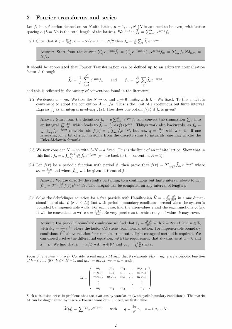
2 Fourier transforms and series

Let fn be a function defined on an N -site lattice, n = 1, . . . , N (N is assumed to be even) with lattice

spacing a (L = Na is the total length of the lattice). We define fq =∑Nn=1 e

iqnafn.

2.1 Show that if q = 2πkNa , k = −N/2 + 1, . . . , N/2 then fn = 1

N

∑q fq e

−iqna.

Answer: Start from the answer∑q e−iqnafq =

∑q e−iqna∑

m eiqmafm =

∑m fmNδn,m =

Nfn.

It should be appreciated that Fourier Transformation can be defined up to an arbitrary normalizationfactor A through

fq =1

A

N∑n=1

eiqnafn and fn =A

N

∑q

fq e−iqna,

and this is reflected in the variety of conventions found in the literature.

2.2 We denote x = na. We take the N → ∞ and a → 0 limits, with L = Na fixed. To this end, it isconvenient to adopt the convention A = 1/a. This is the limit of a continuous but finite interval.

Express fq as an integral involving f(x). How does one obtain f(x) if fq is given?

Answer: Start from the definition fq = a∑Nn=1 e

iqnafn and convert the summation∑n into

an integral∫ L

0dxa , which leads to fq =

∫ L0dxf(x)eiqx. Things work also backwards, as fn =

1Na

∑q fqe

−iqna converts into f(x) = 1L

∑q fqe

−iqx, but now q = 2kπL with k ∈ Z. If one

is seeking for a bit of rigor in going from the discrete sums to integrals, one may invoke theEuler-Mclaurin formula.

2.3 We now consider N →∞ with L/N = a fixed. This is the limit of an infinite lattice. Show that in

this limit fn = a∫ +π/a

−π/adq2π fq e

−iqna (we are back to the convention A = 1).

2.4 Let f(τ) be a periodic function with period β, then prove that f(τ) =∑n∈Z fωne

−iωnτ where

ωn = 2πnβ and where fωn will be given in terms of f .

Answer: We use directly the results pertaining to a continuous but finite interval above to get

fωn = β−1∫ β

0f(τ) eiωnτ dτ . The integral can be computed on any interval of length β.

2.5 Solve the Schrodinger equation for a free particle with Hamiltonian H = − ~2

2md2

dx2 in a one dimen-sional box of size L (x ∈ [0, L]) first with periodic boundary conditions, second when the system isbounded by impenetrable walls. For each case, find the eigenvalues ε and the eigenfunctions ψε(x).

It will be convenient to write ε = ~2k2

2m . Be very precise as to which range of values k may cover.

Answer: For periodic boundary conditions we find that εk = ~2k2

2m with k = 2πn/L and n ∈ Z,

with ψεk = 1√Leikx where the factor

√L stems from normalization. For impenetrable boundary

conditions, the above relation for ε remains true, but a slight change of method is required. Wecan directly solve the differential equation, with the requirement that ψ vanishes at x = 0 and

x = L. We find that k = nπ/L with n ∈ N∗ and ψεk =√

2L sin kx.

Focus on circulant matrices. Consider a real matrix M such that its elements Mk` = mk−` are a periodic functionof k − ` only (0 ≤ k, ` ≤ N − 1, and m−1 = mN−1, m0 = mN etc.):

M =

m0 m1 m2 . . . mN−1

mN−1 m0 m1 . . . mN−2

mN−2 mN−1 m0 . . . mN−3

.... . .

...m1 m2 m3 . . . m0

Such a situation arises in problems that are invariant by translation (with cyclic boundary conditions). The matrixM can be diagonalized by discrete Fourier transform. Indeed, we first define

M(q) =∑`

Mk` eiq(k−`) with q =

2π

Nn, n = 1, 2, . . . N.

2

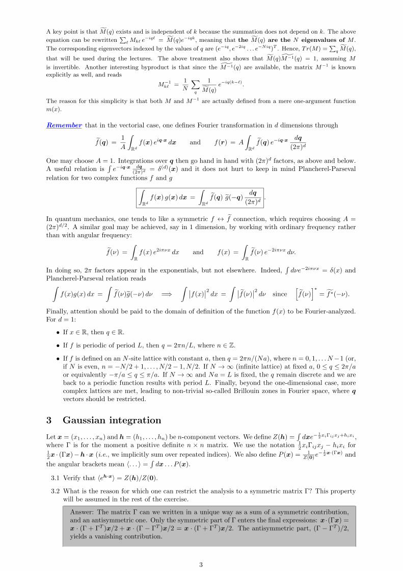
A key point is that M(q) exists and is independent of k because the summation does not depend on k. The above

equation can be rewritten∑

`Mk` e−iq` = M(q)e−iqk, meaning that the M(q) are the N eigenvalues of M .

The corresponding eigenvectors indexed by the values of q are (e−iq, e−2iq . . . e−Niq)T . Hence, Tr(M) =∑

q M(q),

that will be used during the lectures. The above treatment also shows that M(q)M−1(q) = 1, assuming M

is invertible. Another interesting byproduct is that since the M−1(q) are available, the matrix M−1 is knownexplicitly as well, and reads

M−1k` =

1

N

∑q

1

M(q)e−iq(k−`).

The reason for this simplicity is that both M and M−1 are actually defined from a mere one-argument function

m(x).

Remember that in the vectorial case, one defines Fourier transformation in d dimensions through

f(q) =1

A

∫Rdf(x) eiq·x dx and f(r) = A

∫Rdf(q) e−iq·x

dq

(2π)d

One may choose A = 1. Integrations over q then go hand in hand with (2π)d factors, as above and below.A useful relation is

∫e−iq·x dq

(2π)d= δ(d)(x) and it does not hurt to keep in mind Plancherel-Parseval

relation for two complex functions f and g∫Rdf(x) g(x) dx =

∫Rdf(q) g(−q)

dq

(2π)d.

In quantum mechanics, one tends to like a symmetric f ↔ f connection, which requires choosing A =(2π)d/2. A similar goal may be achieved, say in 1 dimension, by working with ordinary frequency ratherthan with angular frequency:

f(ν) =

∫Rf(x) e2iπνx dx and f(x) =

∫Rf(ν) e−2iπνx dν.

In doing so, 2π factors appear in the exponentials, but not elsewhere. Indeed,∫dνe−2iπνx = δ(x) and

Plancherel-Parseval relation reads∫f(x)g(x) dx =

∫f(ν)g(−ν) dν =⇒

∫ ∣∣f(x)∣∣2 dx =

∫ ∣∣f(ν)∣∣2 dν since

[f(ν)

]∗= f∗(−ν).

Finally, attention should be paid to the domain of definition of the function f(x) to be Fourier-analyzed.For d = 1:

• If x ∈ R, then q ∈ R.

• If f is periodic of period L, then q = 2πn/L, where n ∈ Z.

• If f is defined on an N -site lattice with constant a, then q = 2πn/(Na), where n = 0, 1, . . . N−1 (or,if N is even, n = −N/2 + 1, . . . , N/2− 1, N/2. If N →∞ (infinite lattice) at fixed a, 0 ≤ q ≤ 2π/aor equivalently −π/a ≤ q ≤ π/a. If N →∞ and Na = L is fixed, the q remain discrete and we areback to a periodic function results with period L. Finally, beyond the one-dimensional case, morecomplex lattices are met, leading to non-trivial so-called Brillouin zones in Fourier space, where qvectors should be restricted.

3 Gaussian integration

Let x = (x1, . . . , xn) and h = (h1, . . . , hn) be n-component vectors. We define Z(h) =∫dxe−

12xiΓijxj+hixi ,

where Γ is for the moment a positive definite n × n matrix. We use the notation 12xiΓijxj − hixi for

12x · (Γx)−h ·x (i.e., we implicitly sum over repeated indices). We also define P (x) = 1

Z(0)e− 1

2x·(Γx) and

the angular brackets mean 〈. . . 〉 =∫dx . . . P (x).

3.1 Verify that 〈eh·x〉 = Z(h)/Z(0).

3.2 What is the reason for which one can restrict the analysis to a symmetric matrix Γ? This propertywill be assumed in the rest of the exercise.

Answer: The matrix Γ can we written in a unique way as a sum of a symmetric contribution,and an antisymmetric one. Only the symmetric part of Γ enters the final expressions: x ·(Γx) =x · (Γ + ΓT )x/2 + x · (Γ − ΓT )x/2 = x · (Γ + ΓT )x/2. The antisymmetric part, (Γ − ΓT )/2,yields a vanishing contribution.

3

3.3 Prove that

1

2x · (Γx)− h · x =

1

2(x− Γ−1h) · [Γ(x− Γ−1h)]− 1

2(Γ−1h) · [Γ(Γ−1h)]. (1)

Show then that〈eh·x〉 = e

12h·(Γ

−1h). (2)

Answer: The first equality can be found by expanding the right-hand side. Then, we write〈eh·x〉 = Z(0)−1

∫dx e−

12x·(Γx)+h·x, which we cast in the form

〈eh·x〉 = e12h·(Γ

−1h)Z(0)−1

∫dx e−

12y·(Γy),

where y = x− Γ−1h. Changing the integration variable from x to y is just a translation (with

unit Jacobian) and thus 〈eh·x〉 = e12h·(Γ

−1h), by definition of Z(0).

3.4 (side step). With our choice for P above, P (x) = P (−x), so that 〈x〉 = 0. Had we included the

field term in h · x inside our weight, to define a new probability density P ′(x) ∝ e−12xiΓijxj+hixi ,

show that the resulting mean value would have been 〈x〉′ = Γ−1h, where the prime refers to theprobability law used for computing the mean.

Answer: This is a consequence of relation (1), directly stemming from symmetry. The pdf isinvariant under the change x− Γ−1h→ −

(x− Γ−1h

).

3.5 In order to establish that Z(0) = (2π)n/2√det Γ

, we introduce the eigenvalues λ1, . . . , λn of Γ. We define

the diagonal matrix D =

λ1

. . .

λn

, and we denote by Q the matrix such that Γ = QDQT .

By changing variables from x to y = Q−1x, find the announced expression for Z(0).

Answer: Given Γ has been assumed symmetric we know that not only Q exists but it alsoverifies QT = Q−1. This ensures in particular that the Jacobian of the change of variable from

x to y is unity, as |detQ| = 1. As a result Z(0) =∫dye−

12yiDijyj =

∏i

(∫dyie

− 12yiλiyi

)=∏

i

(√2πλi

)= (2π)n/2√

det Γ

3.6 Let Gij = 〈xixj〉. Prove that Gij =∂2 lnZ(h)

∂hi∂hj

∣∣∣∣h=0

.

The relation is true irrespective of the specific form chosen for P . We shall meet it once morein exercise 5, question 2.

3.7 Show then that G = Γ−1.

Answer: Once we know thatGij = ∂2 lnZ(h)∂hi∂hj

∣∣∣h=0

, or, equivalently, thatGij = ∂2 lnZ(h)/Z(0)∂hi∂hj

∣∣∣h=0

,

we use that lnZ(h)/Z(0) = 12h · (Γ

−1h), which we differentiate with respect to hi and thenhj .

3.8 More difficult; skip if short on time. Show that Gij = −2∂ lnZ(0)∂Γij

. Using that ∂ det Γ∂Γij

= det Γ(Γ−1)ji,

get to the same conclusion that G = Γ−1.

Answer: To prove that ∂ det Γ∂Γij

= det Γ(Γ−1)ji for a given pair (i, j), we introduce E, an n × nmatrix whose elements are all zero, except for the (i, j) one, Eij = ε. By definition, ∂ det Γ

∂Γij=

limε→01ε (det(Γ + E) − det Γ). We use that det(I + Γ−1E) = 1 + Tr(Γ−1E) + O(ε2) = 1 +

ε(Γ−1)ji +O(ε2) to conclude.

3.9 Skip if short on time, but stare at the result a little while. Prove that〈x1x2x3x4〉 = G12G34 +G13G24 +G14G23.

4

Answer: Since 〈x1x2x3x4〉 = Z(0)−1 ∂4Z(h)∂h1∂h2∂h3∂h4

∣∣∣h=0

, we also have that

〈x1x2x3x4〉 =∂4e

12h·(Γ

−1h)

∂h1∂h2∂h3∂h4

∣∣∣∣∣h=0

.

This is a tedious but straightforward derivation.

Using the same method as above, one can show that an arbitrary average 〈xi1 . . . xi2m〉 can be writ-ten in terms of the elements of G. This result is known as Wick’s theorem. The idea goes as as fol-lows. Consider first a pairing of the indices {i1, . . . , i2n}, namely a (non ordered) set of n pairs madeof the 2n original indices, which we write {(j1, j2), (j3, j4), . . . , (j2n−1, j2n)}. Take now the productof all the Gj1,j2 . . . Gj2n−1,j2n . One obtains 〈xi1 . . . xi2m〉 as the summation over all possible pairings{(j1, j2), (j3, j4), . . . , (j2n−1, j2n)} of Gj1,j2 . . . Gj2n−1,j2n . There are altogether (2n− 1)!! = (2n− 1)(2n−3) . . . 1 such pairings, and thus as many terms in the summation. For instance with n = 3 (6 indices), onecan form 5× 3 = 15 pairings.

The following manipulations will be reviewed during the lectures and tutorials. They are not, strictlyspeaking, prerequisites. We now turn to a direct application in terms of fields living in continuum space.Below, Dm is then a shorthand for dm1dm2...dmN , for a scalar field m defined on a N -site lattice, takingfurthermore the limit N → ∞. The resulting object is called a functional integral and to tame such aconstruction, be discrete and think of Dm as referring to a finite but large product dm1dm2...dmN . Whendealing with a vectorial field m as in the remainder, the product defining Dm should be considered forall n components of m. Beware also that from now on, x no longer is a Gaussian vector, but simply aposition in space that now plays a role similar to the index i = 1, . . . , N in the lattice case.

3.10 Let Z[h] =∫Dm e−H[m]+

∫dxh(x)·m(x), where H[m] =

∫Lddx(

12∂µmi∂µmi + t

2mimi

)and pe-

riodic boundary conditions in space are assumed (space integrals run over a cubic volume Ld).One should keep in mind that in the discrete formulation on a lattice, we are back to a Gaus-sian problem of the same type as above, with an appropriate choice for the matrix Γ. Hence,“m” can be viewed as a (infinite) collection of vectorial correlated Gaussian variables, each ofthem being m(x), where x is a continuous coordinate. The index µ = 1, . . . , d refers to a spacedirection while i = 1, . . . , n refers to a component of m and summation over repeated indicesis implied as earlier. Verify that with Γi,i′(x,x

′) = δi,i′δ(d)(x − x′) (−∆x + t) we then have

H = 12

∫Lddx dx′

∑i,i′ mi(x) Γi,i′(x,x

′)mi′(x′). Our next goal is to compute the correlation func-

tion Gi,i′(x,x′) = 〈mi(x)mi′(x

′)〉, and related quantities.

Here, it helps to keep in mind that ∇2δ = δ∇2.

3.11 Going to Fourier space, show that Γi,i′(q, q′) = δi,i′ (2π)d δ(d)(q + q′) (q2 + t).

Answer: We Fourier transform Γ with respect to x and x′ to get the desired expression

Γi,i′(q, q′) = δi,i′

∫dxdx′δ(d)(x− x′) (−∆x + t) eiq·x eiq

′·x′ = δi,i′

∫dx(q2 + t) ei(q+q′)·x

= δi,i′ (q2 + t) (2π)d δ(d)(q + q′).

Note that the Laplacian in the first line should be computed before the δ-constraint is applied.When Dirac distribution and differential operators are mixed, one has to ge back to Diracdistribution acting on mere functions, as done here. a

aAs a related exercise, convince yourself that∫dx′f(x′)δ(x− x′)∂x′ (xx′) = xf(x). The direct calculation is

straightforward. Yet, an integration by parts is instructive although cumbersome. This gives

−∫dx′xx′∂x′ [δ(x− x′)f(x′)] = −x

∫x′{f ′(x′)δ(x− x′) + f(x′)∂x′δ(x− x′)}

= −x2f ′(x) + x

∫dx′δ(x− x′)∂x′ (x′f(x′))

= ����−x2f ′(x) +����x2f ′(x) + xf(x).

3.12 Note that Γ is an operator and not a matrix anymore. Let G = Γ−1. The equation defining thecomponents of G is

∑i′

∫dx′ Γi,i′(x,x

′) Gi′,i′′(x′,x′′) = δi,i′′ δ

(d)(x′′−x). Deduce from this result

5

that Gi,i′(q, q′) = (2π)d δ(d)(q + q′) δi,i′ (q

2 + t)−1. This is telling us that the correlation functionreads

Gi,i′(x,x′) =

⟨mi(x)mi′(x

′)⟩

= δi,i′

∫dq

(2π)deiq·(x−x

′)

q2 + t. (3)

Answer: We start from Plancherel-Parseval relation:∫dx′ Γi,i′(x,x

′) Gi′,i′′(x′,x′′) =

∫dq′

(2π)dΓi,i′(x,−q′) Gi′,i′′(q′,x′′)

being somewhat cavalier with notation (the arguments of the functions tell us if we deal withan object in real space, in Fourier space, or mixed as on the rhs). We subsequently Fouriertransform ∑

i′

∫dq′

(2π)dΓi,i′(x,−q′) Gi′,i′′(q′,x′′) = δi,i′′ δ

(d)(x′′ − x)

with respect to x and x′′:∑i′

∫dq′

(2π)dΓi,i′(q,−q′) Gi′,i′′(q′, q′′) = δi,i′′ (2π)d δ(d)(q + q′′).

Inserting the above expression for Γi,i′(q, q′) yields Gi,i′(q, q

′) = (2π)dδ(d)(q+q′)δi,i′/(q2 + t).

Thus,

Gi,i′(x,x′) =

⟨mi(x)mi′(x

′)⟩

=

∫dq

(2π)ddq′

(2π)d(2π)d δ(d)(q + q′) δi,i′

1

q2 + teiq·x+q′·x′

= δi,i′

∫dq

(2π)deiq·(x−x

′)

q2 + t.

Note that the function x 7→∫

dq(2π)d

exp(iq·x)q2+t is not defined at x = 0 (except in d = 1) due

to a large q divergence. In condensed-matter physics, this divergence is an artifact of thecontinuum space limit from which we started. At large q, or equivalently at short distances,the continuum expression is simply not valid. For instance, magnetization is carried by ionsliving on an underlying lattice structure. In polymer or liquid-crystal physics, the short-distancecut-off signalling the breakdown of the continuum limit is played by the elementary monomersize or by the molecular size, respectively. Hence, if the short distance behavior is needed, onemust return to a description going beyond the continuum limit valid only at scales large withrespect to the microscopic ones.

3.13 Show that in the absence of an external magnetic field, 〈m(x) ·m(y)〉 = n∫

dq(2π)d

eiq·(x−y)

q2+t .

Answer: Comes straightforwardly from 〈m(x) ·m(y)〉 =∑iGi,i(x,y).

3.14 What is the effect of having a non vanishing external field h(x) (no calculations asked)? Compute

then 〈m(x)〉 as a function of h(q). What happens if h is uniform?

Answer: Not much changes, as long as we work with the “shifted” field m − 〈m〉, with meanvalue subtracted. For computing this mean value, we use the discrete result of question 4 above(〈x〉 = Γ−1h with the relevant weight), but we have to pay some attention in mapping discretesums with integrals. The counterpart of Γijmimj (implicit summation over repeated indices asalways) is

∫dxdx′m(x)m(x′) . . . and we can proceed, writing

〈mi(x)〉 =∑i′

∫dx′Gi,i′(x,x

′)hi′(x′) =

∫dq

(2π)deiq·x

q2 + thi(−q).

This simplifies into 〈m〉 = h/t when h is uniform. This can be recovered directly fromthe simpler description where all gradient terms in our Hamiltonian are dropped, restrictingourselves to x-independent fields m. We then have H = V tm2/2 − V h ·m where V is thesystem’s volume, which drops out from the calculation of the mean value.

3.15 If j is an n-component constant vector and h = 0, show that

〈e j·m(x)〉 = e j2G(0)/2,

6

where G is given by Eq. (4) below. The latter is not always well defined ; this depends on space dimension.

For instance, a divergent G(0) would be an artifact of our continuous space description.

Answer: We have shown that for a Gaussian discrete vectorial variable X, of 0-mean, 〈exp(H ·X)〉 = exp(HiGijHj/2) where Gij is the correlation function 〈XiXj〉. This result is generalizedhere to the continuous case:

〈e j·m(x)〉 = 〈e∫H(x′)·m(x′) dx′〉 = e

12

∫dydy′Hi(y)Gij(y,y

′)Hj(y′) = e

12

∫dydy′Hi〈mi(y)mj(y

′)〉Hj ,

with Hi(y) = ji δ(d)(y−x). This simplifies into 〈e j·m(x)〉 = e

12 j

2G(0) where G(0) =∫

dq(2π)d

1q2+t .

We have already discussed in the correction of question 12 that in practice this Fourier integral,which is based on the use of a continuum limit, is not always appropriate (G(0) diverges ford ≥ 2). Instead, one must resort to an expression in which the Fourier transform lives on alattice. Spatial derivatives become finite differences. On a cubic lattice, this has the effect of

replacing q2 with a−2(

2− 2d

∑dµ=1 cos(qµa)

)(whose a → 0 limit is indeed q2), and

∫dq

(2π)d

becomes∑

q with the q components being now quantized as in question 1 of section 2.To be specific, we discuss the case d = 1 and for n = 1, where there is actually no short-distancesingularity so that the discrete and continuous descriptions should match if appropriately com-pared. Instead of H[m] =

∫dx[(∂xm)2 + tm2

]/2, one would have here

H[m] = a−1∑x

{1

2[m(x+ a)−m(x)]

2+ a2 t

2m2(x)

}

with x = ja and j = 0, . . . , N−1 is a site index; then one finds G(x) = aN

∑q

eiqx

ta2+2−2 cos qa with

q = 2kπNa , k = −N/2+1, . . . , N/2. In the largeN limit, we arrive atG(x) = a2

∫ π/a−π/a

dq2π

eiqx

ta2+2−2 cos qa

and G(0) = [t(4+ta2)]−1/2. It is also possible to determine the difference G(x)−G(0) as t→ 0+

on a finite lattice: limt→0+(G(x = ja)−G(0)) = −a j(N−j)2N where j = 0, . . . , N − 1.In the next exercise, we will compute a related G(x), that given by Eq. (4) for d = 1, associatedto the Hamiltonian

∫dx[(∂xm)2 + tm2

]/2, which yields 1/(2

√t) when evaluated at x = 0.

This is fully compatible with our [t(4 + ta2)]−1/2 result above for G(0), taking a→ 0..

3.16 Under the same condition, show that

〈e j·[m(x)−m(x′)]〉 = ej2G(0)−j2G(x−x′).

Answer: We could proceed as in the previous question by defining an ad hoc field

h(y) = j(δ(d)(y− x)− δ(d)(y− x′)

)and by writing that 〈e j·[m(x)−m(x′)]〉 = e

12

∫dydy′hi(y)Gij(y,y

′)hj(y′). An alternative is to note

that m(x) − m(x′) is yet another Gaussian variable (not a collection thereof, but a meren-dimensional such vector) and to invoke the cumulant property⟨

ej·[m(x)−m(x′)]⟩

= e j`K`p jp /2

where K`p =⟨[m`(x)−m`(x

′)][mp(x)−mp(x′)]⟩

= δ`p [2G(0)− 2G(x− x′)] with G(x− x′)defined as in the rhs of Eq. (3), but without the δi,i′ (see Eq. (4) below). Hence⟨

ej·[m(x)−m(x′)]⟩

= e[j2G(0)−j2G(x−x′)].

We note that for |x− x′| → ∞, the above result reduces to ej2G(0) = 〈e j·m(x)〉2, as it should.

Two technical side comments. To show the Wick theorem, one can use repeatedly the identity, valid for Gaussianvariables and any function f :

〈xi f(x)〉 =∑j

〈xixj〉⟨∂f

∂xj

⟩.

In addition, the key result 〈xixj〉 = (Γ−1)ij can be recovered by the following trick, arguably the most expedient.We start by endowing our Gaussian vector x with a mean, denoted a:

a` = N∫dxx` exp

(−1

2Γij(xi − ai)(xj − aj)

),

7

where N is the normalization factor, independent of a. Taking the derivative wrt ak, we get

δk` = N∫dxx` Γkm(xm − am) exp

(−1

2Γij(xi − ai)(xj − aj)

).

Taking now a = 0, this yields δk` = Γkm〈xmx`〉, or equivalently 〈xmx`〉 = (Γ−1)m`.

Remember that for a Gaussian distribution with probability density P (x1, . . . xn) ∝ exp(−Γij xixj/2),it is the matrix inverse of Γ that gives the covariances as 〈xixj〉 = (Γ−1)ij . Two other properties are alsooften useful. First the cumulant generating relation∫

Rn dx1 . . . dxn exp(− 1

2Γij xixj + hixi)∫

Rn dx1 . . . dxn exp(− 1

2Γij xixj) = exp

[ 1

2hi (Γ−1)ij hj

].

Second, Wick’s theorem according to which higher order mean values follow from tracking all possiblepairing of the corresponding indices:

〈x1x2x3x4〉 = 〈x1x2〉〈x3x4〉+ 〈x1x3〉〈x2x4〉+ 〈x1x4〉〈x2x3〉.

This implies in particular that 〈x4i 〉 = 3〈x2

i 〉2. When dealing with a Gaussian vector (or variable) ofnon-vanishing mean, one has first to shift x by its mean value to use the above results. This means inparticular that 〈xixj〉 − 〈xi〉〈xj〉 = (Γ−1)ij . Note finally that the cumulant property implies that thecumulant generating function stops at order 2, a distinctive feature of Gaussian variables:

〈ehX〉 = eh〈X〉+h2

2 〈X2〉c ,

where 〈X2〉c is the variance (second cumulant).Important. When dealing with Gaussian fields (infinite collection of variables), and in case of doubt, it isalways possible to go back to the discrete formulation with a Gaussian vector having a large number ofcomponents.Finally, correlation functions of the type

G(x) =

∫dq

(2π)deiq·x

q2 + t(4)

are often met in statistical physics, since they arise within a Gaussian description. Computing such anintegral is feasible with the residue theorem, in dimension d = 1 (see next exercise) and d = 3 where ityields

G(r) =1

4πre−r√t.

In other space dimensions, the result is more involved. It is in particular wrong to write G(r), as sometimes

found, as e−r√t/rd−2, up to some constant. Such an expression does not even give the right large r

behavior.

4 Green’s functions

You may have encountered Green’s function when trying to solve a linear problem involving a field createdby some sources (for instance, in the case of the Poisson equation −∆φ = ρ

ε0where the charge density ρ

is given, and you try to compute the electrostatic potential φ). The connection with the previous sectionis the following. Take a Gaussian variable x with an energy function 1

2x · (Γx) − h · x. If the externalfield h is zero, then of course 〈x〉 vanishes as well. However, if h 6= 0, then 〈x〉 takes a nonzero value. Itis not hard to realize that Γ〈x〉 = h: this is a linear problem with a source h driving a nonzero response〈x〉. Finding the response involves inverting Γ: 〈x〉 = Gh, where G = Γ−1 is the Green’s function. It isalways good to have a small mental library of common Green’s functions. If Γ(x,x′) is an operator, thefact that G(x,x′) is its Green’s function means that

∫dyΓ(x,y)G(y,x′) = δ(d)(x − x′). The Green’s

function G can be a distribution.

4.1 We seek for G when Γ(x,y) = δ(d)(x−y)(−∆x+r). Such a Γ appears in a number of contexts, fromparticle physics to condensed or soft matter. In the present case, we have that (−∆x + r)G(x,y) =δ(d)(x−y). This differential equation admits a solution that is translation invariant, G(x−y). Finda Fourier representation of G.

Answer: We Fourier-transform the differential equation to get G(x− y) =∫

dq(2π)d

eiq·(x−y)

q2+r .

4.2 Compute the explicit form of G(x − y) in the d = 1 case in real space, for r > 0 and then forvanishing r.

8

Answer: We find (e.g., using a contour integral) Gr(x−y) = e−√r|x−y|

2√r

for r > 0 and G0(x−y) =

− 12 |x−y| for r = 0. The latter corresponds to the one-dimensional Coulomb potential (think e.g.

of the potential created by an infinite uniformly charged plate, which is linear in the distancex to the plate. Yet, some care is required since we face a divergence when r = 0. For a direct

calculation, we can regularize the divergence at q = 0, to compute G0(x) = −∫dq2π

1−cos(qx)q2 .

Changing variable to q = q|x| (attention should be paid to the sign of x, that may interchangethe boundaries of integration), we get

G0(x) = −|x|∫

dq

2π

1− cos(q)

q2= −|x|

2.

To compute the last integral, we integrate by parts :∫dq(1− cos q)/q2 =

∫dq(sin q)/q = π.

4.3 Let Γ(t, t′) = δ(t− t′) ddt′ . Find G(t, t′).

Answer: G(t, t′) = Θ(t− t′) is the Heaviside step function.

We finish with two more examples that connect with other areas of physics. First, Γ(x, t;x′, t′) = δ(t− t′)δ(x−x′)[

∂∂t−D ∂2

∂x2

], with D > 0. This yields the heat equation, that admits the diffusion kernel

G(x, t;x′, t′) = Θ(t− t′) e− (x−x′))2

4D(t−t′)√4πD(t− t′)d

as a Green’s function. The step function makes causality explicit.

Second, we consider Γ(x, t;x′, t′) = δ(t− t′)δ(x−x′)[

1c2

∂2

∂t2− ∂2

∂x2

], the Green’s function of which turns out to

be problematic. Such a kernel Γ shows up in the Lorentz gauge, where Maxwell’s equations read � ~A = µ0~j and

�φ = ρ/ε0; � is the three dimensional generalization of the wave operator 1c2

∂2

∂t2− ∂2

∂x2 . The question is tricky,

since Γ is strictly speaking not invertible. Depending on the subspace of functions one is working with, it does

admit different Green’s function (advanced, retarded, Feynman).

5 Legendre transform

Let Z(h) =∫dxe−H(x)+x·h be a function of a vector h that can be interpreted as the canonical partition

function of a system characterized by the x degrees of freedom in some external field h. We use acontinuum notation for x, but these could also be discrete variables like Ising spins. The (opposite anddimensionless) free energy is W (h) = lnZ(h). Here, unlike in section 3, we do not assume H to bequadratic.

5.1 Angular brackets 〈. . .〉 denote an average with respect toe−H(x)+x·h

Z(h). Show that 〈xi〉 =

∂W

∂hi

∣∣∣∣.5.2 Show that Gij = 〈xixj〉 − 〈xi〉〈xj〉 =

∂2W

∂hi∂hj

∣∣∣∣.5.3 Let ξi(h) = ∂W

∂hi. We denote by hi(ξ) the inverse function giving h as a function of ξ and we define

Γ(ξ) = ξ · h −W (h) but what we really mean is Γ(ξ) = ξ · h(ξ) −W (h(ξ)). This Γ depends on ξonly. It is the Legendre transform of −W (see the comment below for the sign convention). Showthat ∂Γ/∂ξi = hi.

Answer: dΓ = −dW + hidξi + ξidhi = hidξi.

5.4 Let Γij = ∂2Γ∂ξi∂ξj

evaluated at ξ = 〈x〉. Prove that G = Γ−1.

Answer: We start from ∂Γ∂ξi

= hi and we differentiate a second time wrt ξj :∂2Γ∂ξj∂ξi

= ∂hi∂ξj

. But

given that ∂hi∂ξj

Gjk = ∂hi∂ξj

∂ξj∂hk

= δik, we have found that indeed ΓG is the identity matrix.

Physical meaning of Γ(ξ): In much the same way as W is the proper thermodynamic potential at fixed h,we can see Γ as the thermodynamic potential in the conjugate ensemble in which one would be working atfixed average 〈x〉. In a more standard language, in the canonical ensemble F (V ) = −kBT lnZ(V ) is thefree energy at fixed volume and the pressure is P = − ∂F

∂V , but working in the isobaric ensemble leads to

9

the free enthalpy G(P ) = F + PV being the natural potential, which verifies 〈V 〉 = ∂G∂P . In the magnetic

language, these results apply as well (fixed magnetic field versus fixed magnetization).

Remember that there exist a number of variants for defining the Legendre transform, with differentconventions. A common choice, starting from a function f(h) is to define Γ = f(h)− hf ′(h), understoodas a function of “the slope” ξ = f ′(h). It is then important that f be convex, so that h can be expressedunivocally as a function of ξ. A similar convexity requirement should hold in the vectorial case, as treatedabove (where Γ is the Legendre transform of −W ).In the mathematical literature, Legendre transformation is defined seemingly differently, through Γ(ξ) =minh[f(h)− h ξ], for a convex-up function f(h). For a given ξ, the minimum is reached for f ′(h) = ξ andthis definition coincides with the “physicist” one, with the bonus of a compact notation. One also findsthe definition Γ(ξ) = maxh[h ξ − f(h)], which changes a few signs, but makes sure that the transform isconvex-up itself, and can be itself Legendre transformed one more time to yield back the original f(h).Geometrical interpretation: Γ = f(h)− hf ′(h) is nothing but the y-intercept of the tangent to the graphof f at abscissa h. This quantity Γ, expressed as a function of the slope f ′(h) = ξ, can then be sketchedgraphically as in the picture below (it is useful to train oneself to be able to perform graphically thetransformation). The Legendre transform is an important tool in thermodynamics, statistical physics andanalytical mechanics.Further reading : Making Sense of the Legendre Transform by Zia et al., https://arxiv.org/abs/0806.1147.

6 Functional derivatives

Let q(t) be a function of t and let S[q] be a functional of q. The functional derivative of S wrt q(t0) isdefined as follows. Let qε,t0(t) = q(t) + εδ(t − t0), then δS

δq(t0) = limε→01ε (S[qε,t0 ] − S[q]). Another way

to put it is that when q → q + δq (meaning that the trajectory q(t) is perturbed by δq(t)), the functionalchanges from S to S + δS, with

δS =

∫δS

δq(t′)δq(t′) dt′, (5)

to first order in δq. This relation defines the functional derivative δS/δq(t′), which is a functional of q anda function of t′.

6.1 What is δq(t1)δq(t2)?

Answer: δ(t1 − t2), as obtained from the two definitions.

6.2 If S can be written in the form S[q] =∫∞

0dtL(q(t), q(t)), where L is a function of q(t) and q(t), prove

that δSδq(t0) = ∂L

∂q −ddt∂L∂q where everything is evaluated at t = t0. In mechanics, L is a Lagrangian

while S is an action.

Answer: We apply the definition and start from S[qε,t0 ] =∫dtL(qε,t0 , qε,t0) which we expand

to first order in ε: S[qε,t0 ] = S[q] + ε∫dt[δ(t− t0)∂L∂q + δ(t− t0)∂L∂q

]. After an integration by

parts and after using the δ(t−t0) distribution, we thus arrive at S[qε,t0 ]−S[q] = ε[∂L∂q −

ddt∂L∂q

],

which is the desired result.

6.3 If now S[φ] is a functional of a field φ living in d-dimensional space, such that S[φ] =∫dxL(φ, ∂µφ),

(where µ = 1, . . . , d refers to space directions), explain why δSδφ(x0) = ∂L

∂φ − ∂µ∂L∂∂µφ

(at x0).

10

Answer: After defining φε,x0(x) = φ(x) + εδ(d)(x − x0) we repeat the procedure sketched in

the previous section and arrive at the Euler-Lagrange equations for the field φ (with t → x,q → φ and d

dt →∇·.

6.4 Let S[φ] =∫dx

(12

(dφdx

)2

+ r2φ

2

). Determine δS

δφ(x1) and then δ2Sδφ(x2)δφ(x1) .

Answer: δSδφ(x1) = −d

2φdx2 (x1) + rφ(x1) and thus δ2S

δφ(x2)δφ(x1) = δ(x1 − x2)[− d2

dx21

+ r]. Note that

for any distribution T , ∇2T = T ∇2.

Remember the connection between functional derivatives and Euler-Lagrange equations. Besides, ourfirst order expansion Eq. (5) can be pushed one order higher:

δS = S[q + δq]− S[q] =

∫δS

δq(t′)δq(t′) dt′ +

1

2

∫δ2S

δq(t′)δq(t′′)

∣∣∣∣q

δq(t′) δq(t′′) dt′ dt′′.

Side comment: functional derivatives and functional integrals have nothing to do with each other, in thesense that our introductory discussion does not involve any functional integration, but simple integrationinstead.

7 Pauli matrices (Soft Matter track can skip)

Let σ1,2,3 be the Pauli matrices σ1 =

[0 11 0

], σ2 =

[0 −ii 0

], σ3 =

[1 00 −1

], and σ0 be the 2-by-2 identity.

Remember that the Pauli matrices satisfy the algebra σ`σn = δ`n σ0 + i

∑3j=1 ε`njσ

j (`, n ∈ {1, 2, 3})and the commutation relations [σ`, σn] = 2i

∑3j=1 ε`njσ

j , where δ`n is the Kronecker delta (δ`n is nonzeroonly if ` = n, in which case it is equal to 1) and ε`nj is the (antisymmetric) Levi-Civita symbol (ε`nj isnonzero only if the three indices are different; in that case, it is equal to (−1)p, where p is the numberof transpositions that bring {`, n, j} into {1, 2, 3}). In short, [σ1, σ2] = 2iσ3 (plus permutations, as forangular momentun operators, which they almost are). Besides, (σ1)2 = (σ2)2 = (σ3)2 = σ0 = I and thematrices anticommute σ1σ2 + σ2σ1 = 0, etc. Thus, σ1σ2 = i σ3, σ2σ3 = i σ1 etc.

7.1 Show that, for any real number λ and vector ~v with real components, the eigenvalues µ± of Mλ,~v =

λσ0 + ~v · ~σ def= λσ0 +

∑3j=1 vjσ

j are µ± = λ± |~v|, where |~v| =√v2

1 + v22 + v2

3 .

Answer: The eigenvalues can be determined by computing the trace of Mλ,~v and of M2λ,~v. The

result is readily obtained using that the Pauli matrices are traceless: tr[Mλ,~v] = µ+ + µ− = 2λand tr[M2

λ,~v] = µ2+ + µ2

− = tr[(λ2 + |~v|2)σ0 + 2λ~v · ~σ] = 2(λ2 + |~v|2).

7.2 Show that Π± =(σ0 ± ~v·~σ

|~v|

)/2 are the projectors on the eigenvectors of Mλ,~v (Π2

± = Π± and

Mλ,~vΠ± = (λ± |~v|)Π±; consequently, one has the spectral decomposition

Mλ,~v = (λ+ |~v|)Π+ + (λ− |~v|)Π−.

Answer: Π2± = Π± because the eigenvalues of

σ0±~v·~σ|~v|2 are {0, 1}. They project on the eigenvec-

tors of Mλ,~v, indeed

Mλ,~vΠ± = (λσ0 + ~v · ~σ)σ0 ± ~v·~σ

|~v|

2= λ

σ0 ± ~v·~σ|~v|

2+~v · ~σ ± (~v·~σ)2

|~v|

2= (λ± |~v|)Π± .

7.3 A function f(M) of a diagonalizable matrix M is the matrix with the same eigenvectors of M andwith eigenvalues f(mi), where mi are the eigenvalues of M . Calculate Tr[(tanh(sin(~v · ~σ))7].

Answer: Every odd function of the Pauli matrices is traceless.

7.4 Show that, if ~v · ~w =∑3j=1 vjwj = 0, then eλ~v·~σ ~w · ~σ = ~w · ~σ e−λ~v·~σ.

11

Answer: Using the spectral decomposition of ~v · ~σ, we find eλ~v·~σ = eλ|~v|σ0+~v·~σ

|~v|2 + e−λ|~v|

σ0−~v·~σ|~v|2 .

Indeed, ~v · ~σ = vΠ+ − vΠ− with v = |~v|, Π+Π− = 0, exp(λvΠ±) = σ0 +(e±λv − 1

)Π± since

Π2± = Π±. The final result follows from ~v · ~σ ~w · ~σ = −~w · ~σ~v · ~σ.

7.5 Prove

eiπ4

3σ2+4σ3

5 σ1 e−iπ4

3σ2+4σ3

5 =3σ3 − 4σ2

5

(hint: define the vector ~v in such a way that ~v · ~σ = 3σ2+4σ3

5 , what is |~v|?).

Answer: The vector ~v has a magnitude of 1 (|~v| = 1), and it is given by ~v =

03545

. Thus we

have

eiπ4

3σ2+4σ3

5 σ1e−iπ4

3σ2+4σ3

5 = eiπ4 ~v·σσ1e−i

π4 ~v·σ = σ1e−i

π2 ~v·σ ,

where we applied the identity proved in the previous point. We now use the spectral decompo-sition of e−i

π2 ~v·~σ

σ1e−iπ2 ~v·σ = σ1

(e−i

π2 Π+ + ei

π2 Π−

)= σ1

(−iΠ+ + iΠ−

)= −iσ1~v · ~σ =

3σ3 − 4σ2

5.

12