Statistical Machine Learning Approaches

to Change Detection

Song Liu, JSPS DC2,

Sugiyama Lab, Tokyo Institute of Technology

2014/3/10

1

Song Liu (Tokyo Tech)

• Graduating PhD student (3rd year) from Tokyo Tech• Thesis: Statistical Machine Learning Approaches to

Change Detection

• Fellow of Japan Society for Promotion of Science (JSPS)

• Visiting at National Institute of Informatics, JP

• MSc in Advanced Computing (University of Bristol)

• BEng in Computer Science (Soochow University, CN)

2

Learning from Data

• The era of big data is coming.

1 hour video per second 1M transaction per hour 2.5 petabytes per 1000 person

• Without interpretation, raw data make no sense to human.• Machine learning helps make sense out of data.

3

The Human Learning in AstronomyA brief history

• Learning Constellations• Patterns of Stars

• Predicting warfare, harvest

• Patterns of Planetary Movements• Tycho Brahe’s data

• Kepler’s law

• Newton Laws• Predicting the movements of new

planets 4𝐹 = 𝑚𝑎

Statistical Machine Learning

Data is so big, so we look for compressive rules (patterns).

Data involving uncertainty, we prefer statistical patterns .5

However, Data is Always Changing!

• Patterns learned today may be useless tomorrow.

• Learning pattern changes are also important.

• We need a new paradigm of machine learning.

Everyday, 20% Google queries have never been seen before1.

Red spots are detected changes on NASA satellite images, reflecting the heaviest damages after super typhoon Haiyan struck Philippines on Nov. 8 2013 2.

1. http://certifiedknowledge.org/blog/are-search-queries-becoming-even-more-unique-statistics-from-google2. http://www.nasa.gov/content/goddard/haiyan-northwestern-pacific-ocean/#.Uq3u6vQW2So 6

Two Paradigms of Machine Learning

SupervisedPredict future under data shifts

𝑝 𝑦′ 𝒙′ , 𝑝 ≠ 𝑝′

SupervisedPredict Future: 𝑝(𝑦|𝒙)

Classification, Regression (Duda et al., 2001, Bishop, 2006)

UnsupervisedLearn Patterns: 𝑝 𝒙

Clustering, Anomaly Detection (Murphy, 2012, Shaw-Taylor & Cristianini, 2004)

UnsupervisedLearn changes of patterns

𝑝/𝑞 or 𝑝 − 𝑞, 𝑝 ≠ 𝑞

Dynamic Learning: Data are shifting

Static Learning: Data do not change

e.g. Transfer learning (Sugiyama et al., 2012) Change detection 7

(p.5)

Two Ways of Learning Changes

8

①

②

Separated Learning Approach

Direct Learning Approach

Which one is the best ?

Vapnik’s Principle

• Generally, we prefer ② to ① because of Vapnik’sprinciple.

• “When solving a problem of interest, one should not solve a more general problem as an intermediate step.”

(Vapnik, Statistical Learning Theory, 1998)

Support Vector Machines! 9

Unsupervised Change Detection

• Has it been changed? Distributional Change Detection

• What has been changed? Structural Change Detection

In Density Function

Heartbeat disorder detection, from JMOTIF project.

In Graphical Model

Changes in brain activation (Cléry et al., 2006) 10

(p.10)

Chapter 2, Distributional Change Detection

1. Background & Existing Methods2. Problem Formulation3. Divergence based Change-point Score4. Experiments

12

Changes in Time-series

13

Health monitoring

Engineering fault detection

Network intrusion detectione.g. Takeuchi et al., 2006

e.g. Keogh et al., 2005

e.g. Kawahara et al., 2012

Distributional Change Detection in Time-series

• Objective: Detecting abrupt changes lying among time-series data

• Change-point score: Plausibility of changes that have happened

• Metrics: True positive rate, false positive rate, and detection delay

0 200 400 600 800 1000 1200 1400 1600 1800 2000

Sensor Reading

Change-Point Score

14

Existing Methods

• Model based Methods:• Auto Regressive (AR)

• (Takeuchi and Yamanishi, 2006)

• Autoregressive model with Gaussian noise.• Singular Spectrum Transformation (SST)

• (Moskvina and Zhigljavsky, 2003)

• Subspace Identification (SI)• (Kawahara et al., 2007)

• State Space model with Gaussian noise.

• Model-free Methods: • One-class Support Vector Machine (OSVM)

• (Desobry et al., 2005)

• Density Ratio based Methods (KLIEP)• KLIEP (Kawahara & Sugiyama, 2009)

• No model assumption.

-4 -3 -2 -1 0 1 2 3 40

500

1000

1500

2000

2500

3000

-4 -2 0 2 4 6 8 100

500

1000

1500

2000

2500

Model based methods fail to characterize data when model mismatches.

15

modeldata

Chapter 2, Distributional Change Detection

1. Background & Existing Methods2. Problem Formulation3. Proposed Method4. Experiments

16

a c eb d f g h i jTime

Sliding window Imaginary Bar a Time point

Formulate Problem from Time-series• Construct samples by using sliding window.• An imaginary bar in the middle divides samples into two groups. • Assume two groups of samples are from 𝑝 and 𝑞.

17How to generate a change point score?

Chapter 2, Distributional Change Detection

1. Background & Existing Methods2. Problem Formulation3. Proposed Method4. Experiments

18

Divergence based Change Point Detection

• Need a measure of change between 𝑝(𝒙) and 𝑞(𝒙).

• f-divergence is a distance from 𝑝 to 𝑞.

• 𝑓 is a function of a ratio between two probability density functions (𝑝 and 𝑞).

• D[𝑝||𝑞] is asymmetric, thus we symmetrized it:

f is convex

𝑓 1 = 0

19

(Ali and Silvey, 1966)

Density Estimation

• A naive way is a two step approach:

• e.g. Kernel Density Estimation (Csörgo & Horváth 1988)

•① or ② is carried out without taking care of the ratio.• Error may be magnified after the division.

-5 0 5

0

0.5

1

x

p(x

)

𝑝 𝒙; 𝜎 =1

𝑛

𝑖=1

𝑛

𝐾𝜎(𝑥, 𝑥𝑖)

𝐾𝜎 𝒙, 𝒙′ =1

𝜎 2𝜋exp(

𝒙 − 𝒙′2

−2𝜎2)

① 𝑝 𝒙 ≈ 𝑝(𝒙)

② 𝑞 𝒙 ≈ 𝑞(𝒙)

𝑝(𝒙)

𝑞(𝒙)≈

𝑝 (𝒙)

𝑞 (𝒙)

20

• Direct Density Ratio Estimation (Sugiyama et al., 2012).

• By plugging in estimated density ratio, we may obtain various f-divergences.

Density Ratio Estimation

21

Knowing 𝑝

𝑞Knowing 𝑝 and 𝑞

Vapnik’s Principle!

-1.5 -1 -0.5 0 0.5 1 1.50

0.5

1

1.5 𝑝

𝑞𝑞

𝑝

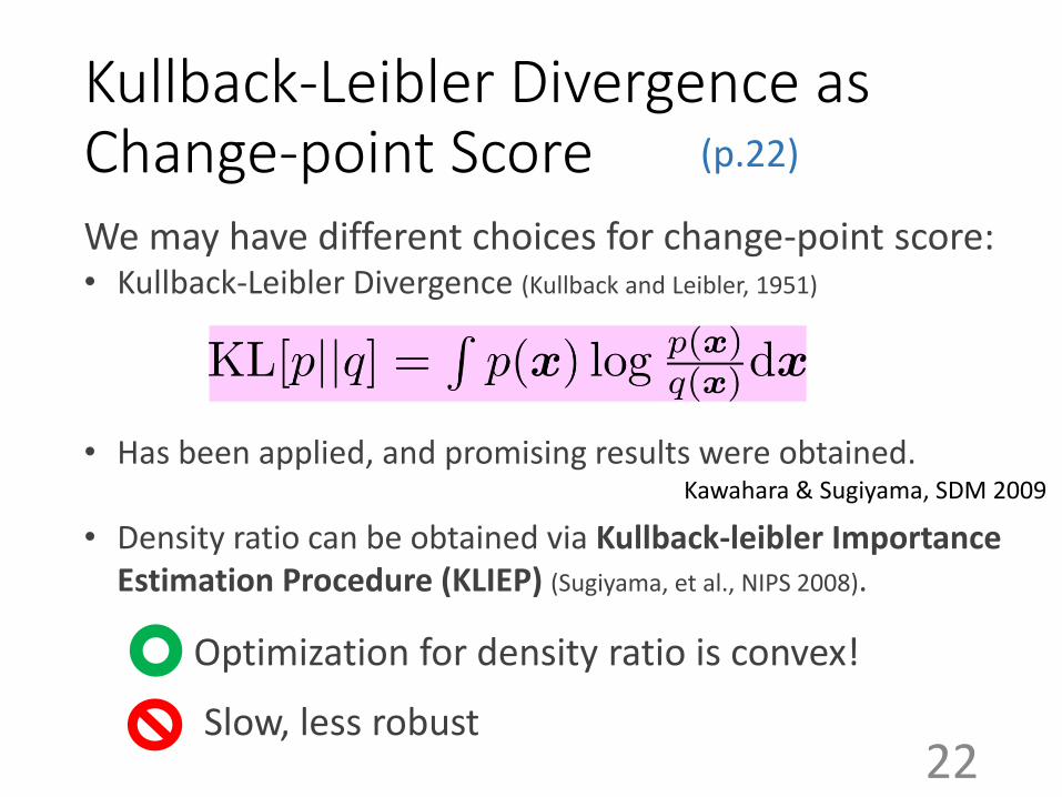
Kullback-Leibler Divergence as Change-point ScoreWe may have different choices for change-point score:• Kullback-Leibler Divergence (Kullback and Leibler, 1951)

• Has been applied, and promising results were obtained.

• Density ratio can be obtained via Kullback-leibler Importance Estimation Procedure (KLIEP) (Sugiyama, et al., NIPS 2008).

Optimization for density ratio is convex!

Slow, less robust

Kawahara & Sugiyama, SDM 2009

22

(p.22)

Pearson Divergence as Change-point Score

• The log term in Kullback-leibler divergence can go

infinity if 𝑝(𝒙)

𝑞(𝒙)= 0.

• Pearson Divergence (Pearson, 1900)

• Density ratio can be obtained via unconstrained Least Square Importance Fitting (uLSIF) (Kanamori, et al., JMLR 2009).

• Solution has an analytic form.

Fast, relatively robust!

23

(pp.24)

Relative Pearson Divergence as Change-point Score• The density ratio may go unbounded.

• Bounded Density Ratio -> Relative Density Ratio

• Relative Pearson Divergence (Yamada, et al. , NIPS 2011)

𝑝

𝛼𝑝+ 1−𝛼 𝑞≤

1

𝛼

𝑝

𝑞

More robust!

-8 -6 -4 -2 00

5

10

15

20

25

24

(pp.26)

Divergences as Change-point Scores (Summary)• Kullback-Leibler Divergence (via KLIEP) :

• Pearson Divergence (via uLSIF):

• Relative Pearson Divergence (via RuLSIF):

Existing method

Robust Change

Detection

Liu et al., SPR 2012, Neural Networks 2013

Previous Work: Kawahara & Sugiyama, 2009

25

(pp.22-28)

Chapter 2, Distributional Change Detection

1. Background & Existing Methods2. Problem Formulation3. Proposed Method4. Experiments

26

Experiments (Synthetic)

27

Mean Shift

Variance Scaling

Covariance Switching

original signal

score

ground truth

Experiments (Sensor)

Mobile Sensor data, measured in 20 seconds, recording human activity.

Stay Walk Jog

time

Task: Segmenting the activities.e.g. walk, jogging, stairs up/down…

False Positive Rate

True Po

sitive Rate

time

HASC 2011 Challenge

28

Experiments (Twitter Messages)

BP Oil Spill

29

Conclusion

• A robust and model-free method for distributional change detection in time-series data was proposed.

• The proposed method obtained the leadingperformance in various artificial and real-worldexperiments.

30

Chapter 3, Structural Change Detection

1. Background 2. Separate Estimation Methods3. Proposed Methods4. Experiments

31

Patterns of Interactions

• Genes regulate each other via gene network.

• Brain EEG signals may be synchronized in a certain pattern.

• However, such patterns of interactions may be changing!

(Wikipedia)

32

Structural Change Detection

• Interactions between features may change.

• e.g. Interactions between some genes may be activated, • but only under some conditions.

• “apple” may co-occur with “banana” quite often in cookbook, • but not in IT news.

The change of brain signal correlation at two different experiment intervals. (Williamson et al., 2012)

33

𝒙 = 𝑥 1 , … , 𝑥 𝑑 T

Chapter 3, Structural Change Detection

1. Background 2. Existing Methods3. Proposed Methods4. Experiments

34

• The interactions between random variables can be modelled by Markov Networks.

• Markov Networks (MNs) are undirected Graphical Models. • The simplest example of MN is a Gaussian MN:

• We can visualize the above MN using an undirected graph.

Gaussian Markov Networks (GMNs)

𝒙 = (𝑥 1 , 𝑥 2 , … , 𝑥(𝑑)) 𝚯 is the inverse covariance matrix

1 23

546 35

Estimating Separate GMN

• Recall, we would like to detect changes between MNs.

• Changes can be found once the structure of two separate GMNs are known to us.

• Estimating Sparse GMNs can be done via Graphical Lasso (Glasso).

• Idea: Twice Glasso, take the parameter difference.

1 23

546

1 23

546

Tibshirani, JRSS 1996; Friedman et al., Biostatistics 2008

36

Glasso: Pros and Cons

Pros:

• Statistical properties are well studied.

• Off-the-shelf software can be used.

• Sparse change is produced.

Cons:

• Cannot detect high-order correlation.

• Not clear how to choose hyper-parameters.

• Does not work if 𝒑 or 𝒒 is dense.

P Q

Change

sparse sparse

sparse

Can we combine two optimizations into one?

37

Semi-direct Approach (Fused-lasso)

• We can impose sparsity directly on , using Fused-lasso (Flasso) (Tibshirani et al., 2005).

• Consider the following objective:

We don’t have to assume 𝑝 or 𝑞 is sparse.

Sparsity control is much easier than Glasso.

Gaussianity is still assumed.

(Zhang & Wang, UAI2010)

38

Gaussian Gaussian

Nonparanormal (NPN) Extension

• Gaussian assumption is too restrictive.

• However, considering general non-Gaussian model can be computationally challenging.

• We may consider a method half-way between Gaussian and non-Gaussian.

• Non-paranormal (NPN).

𝑓𝑘 : Monotone, differentiable function

𝒙 = (𝑥 1 , 𝑥 2 , … , 𝑥(𝑑))

𝒇(𝒙) = (𝑓1(𝑥1 ), 𝑓2(𝑥

2 ), … , 𝑓𝑑(𝑥𝑑 ))

Liu et al., JMLR 2009

39

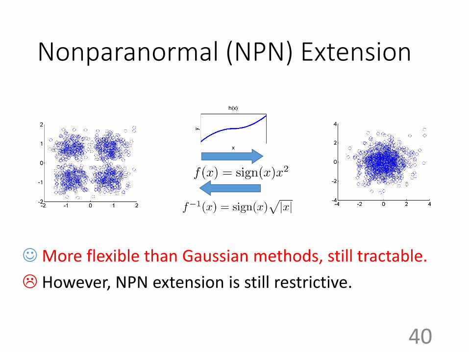
Nonparanormal (NPN) Extension

More flexible than Gaussian methods, still tractable.

However, NPN extension is still restrictive.

40

Non-Gaussian Log-linear Model

• Pairwise Markov Network

• 𝒇 are feature vectors.

• The normalization term 𝑍(𝜽) is generally intractable.• Gaussian or Nonparanormal models are exceptions.

𝒇: ℛ2 → ℛ𝑏

Gaussian: 𝑓𝑔𝑎𝑢 𝑥, 𝑦 = 𝑥𝑦

Nonparanormal: 𝑓𝑛𝑝𝑛 𝑥, 𝑦 = 𝑓 𝑥 𝑓(𝑦)

Polynomial: 𝒇𝑝𝑜𝑙𝑦 𝑥, 𝑦 = [𝑥𝑘 , 𝑦𝑘 , 𝑥𝑘−1𝑦 … , 𝑥, 𝑦, 1]

41

The Normalization Issue

• However, for a generalized Markov Network, there is no closed-form for 𝑍(𝜽).

• Importance Sampling (IS):

• IS can be used to extend both Glasso and Flasso. • IS-Glasso, IS-Flasso.

!

42

Chapter 3, Structural Change Detection

1. Background 2. Existing Methods3. Proposed Methods4. Experiments

43

• Recall, our interest is:

• The ratio of two MNs naturally incorporates the !

Modeling Changes Directly

So, model the ratio directly! 44

Modeling Changes Directly

• Density ratio model:

• The normalization term is:

To ensure: Sample average approximationAlso works when integral has no closed form!

45

𝑝 = 𝑞(𝒙)𝑟 𝒙, 𝜷

Estimating Density Ratio

• Kullback-Leibler Importance Estimation Procedure (KLIEP):

Unconstrained convex optimization!

Sugiyama et al., NIPS 2007

Tsuboi et al, JIP 2009 46

𝑝(𝒙) = 𝑞(𝒙) 𝑟 𝒙

Sparse Regularization

• Impose sparsity constraints on each factor 𝜷𝑢,𝑣.

• equals to impose sparsity on changes.

• So finally, we can obtain a with group sparsity!

L2 regularizers Group lasso regularizer

Elastic Net

𝜷

47

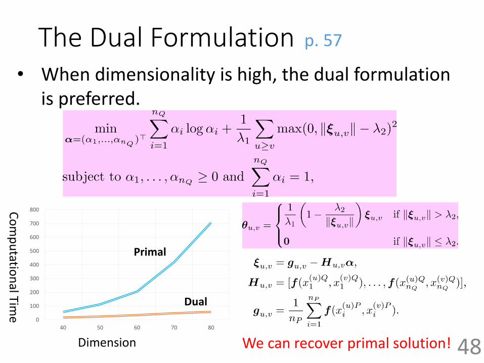
The Dual Formulation

0

100

200

300

400

500

600

700

800

40 50 60 70 80

Primal

Dual

Dimension

Co

mp

utatio

nal Tim

e

• When dimensionality is high, the dual formulation is preferred.

48We can recover primal solution!

p. 57

Summary: Comparison between Methods

49• The Illustration of methods on model assumption

and estimation procedure

Liu et al., ECML 2013, Neural Computation 2014

Chapter 3, Structural Change Detection

1. Background 2. Existing Methods3. Proposed Methods4. Experiments

50

Gaussian Distribution (𝑛 = 100, 𝑑 = 40)

Regularization path

Start from 40 dimensional GMN with random correlations.

Randomly drops 15 edges. Precision and Recall curves are

averaged over 20 runs.

P-R curve

𝜷𝑢,𝑣

𝜷𝑢,𝑣

𝜷𝑢,𝑣

51

Gaussian Distribution (𝑛 = 50, 𝑑 = 40)

P-R curve

Regularization path

Start from 40 dimensional GMN with random correlations.

Randomly drops 15 edges. Precision and Recall curves are

averaged over 20 runs.

𝜷𝑢,𝑣

𝜷𝑢,𝑣

𝜷𝑢,𝑣

52

Diamond Distribution (𝑛 = 5000, 𝑑 = 9)

• The proposed method has the leading performance.

Regularization pathP-R curve

𝜷𝑢,𝑣

53

Twitter Dataset

•We choose the Deepwater Horizon oil spill as the target event.• Samples are the frequencies of 10 related

keywords over time. • Detecting the change of co-occurrences

on keywords before and after a certain event.

source: Wikipedia

54

Q P P P

Twitter Dataset

Time

3 weeks~4.17

…

55

(pp. 68-72)

The Change of Correlation From 7.26-9.14

KLIEP Flasso

56Small # of samples, severe over-fitting of Flasso!

Conclusion

• We proposed a direct structural change detection method for Markov Networks.

• The proposed method can handle non-Gaussian data, and can be efficiently solved using primal or dual objective.

• The proposed method showed the leadingperformance on both artificial and real-world datasets

57