University of South FloridaScholar Commons

Graduate Theses and Dissertations Graduate School

1-1-2015

Statistical Learning with Artificial Neural NetworkApplied to Health and Environmental DataTaysseer SharafUniversity of South Florida, tsharaf@umich.edu

Follow this and additional works at: http://scholarcommons.usf.edu/etd

Part of the Mathematics Commons, and the Statistical Methodology Commons

This Dissertation is brought to you for free and open access by the Graduate School at Scholar Commons. It has been accepted for inclusion inGraduate Theses and Dissertations by an authorized administrator of Scholar Commons. For more information, please contactscholarcommons@usf.edu.

Scholar Commons CitationSharaf, Taysseer, "Statistical Learning with Artificial Neural Network Applied to Health and Environmental Data" (2015). GraduateTheses and Dissertations.http://scholarcommons.usf.edu/etd/5866

Statistical Learning with Artificial Neural Network Applied To

Health and Environmental Data

by

Taysseer Sharaf

A dissertation submitted in partial fulfillmentof the requirements for the degree of

Doctor of PhilosophyMathematics & Statistics

College of Arts and SciencesUniversity of South Florida

Major Professor: Chris P. Tsokos, Ph.D.Kandethody Ramachandran, Ph.D.

Rebecca Wooten, Ph.D.Dan Shen, Ph.D.

Date of Approval:April 9, 2015

Keywords: Statistical Learning, Bayesian Learning for ANN, Artificial Neural Network,Cancer Survival, Global Warming

Copyright © 2015, Taysseer Sharaf

Dedication

This doctoral dissertation is dedicated to my parents (Mahmoud Sharaf and Samiaa

Hassan), my wife (Sara Mahmoud), my Childern (Lujyeen Sharaf, Adam Sharaf and Ryan

Sharaf), and my brothers and sisters.

Acknowledgments

I would like to express my deepest gratitude to my advisor Professor Chris P. Tsokos

for his endless support, motivation, encouragement and advice during my graduate study. I

will be owing him for my success as a researcher and teacher in years to come.

I would like to thank Dr. Kandethody Ramachandran, Dr. Rebecca Wooten, and Dr.

Dan Shen for serving as the member of my Ph.D. committee, continuous support, and con-

structive advice during the preparation of this dissertation and during my study at USF.

Furthermore, many thanks to my friends Dr. Keshav Pokhrel, Dr. Ram Kafle, Dr. Nana

Bonsu and Bhikhari Tharu for their support and advice during the past five years.

Finally, I could not reach this point without the endless support of my beloved wife.

She was always by my side supporting me and encouraging me to do my best. Thank you

Sara for being there for me and taking care of our lovely children when I was not there.

Table of Contents

List of Tables . . . . . . . . . . . . . . . . . . . . . . . . . . . . . . . . . . . . . . iii

List of Figures . . . . . . . . . . . . . . . . . . . . . . . . . . . . . . . . . . . . . . iv

Abstract . . . . . . . . . . . . . . . . . . . . . . . . . . . . . . . . . . . . . . . . . vi

Chapter 1 Introduction . . . . . . . . . . . . . . . . . . . . . . . . . . . . . . . . 11.1 The Use of Artificial Neural Network in Health Sciences . . . . . . . . . . 21.2 Skin Cancer (Melanoma) . . . . . . . . . . . . . . . . . . . . . . . . . . . 31.3 Survival Analysis . . . . . . . . . . . . . . . . . . . . . . . . . . . . . . . 4

1.3.1 Discrete Survival Time . . . . . . . . . . . . . . . . . . . . . . . . 5

Chapter 2 Artificial Neural Networks . . . . . . . . . . . . . . . . . . . . . . . . 112.1 Types of Artificial Neural Networks . . . . . . . . . . . . . . . . . . . . . 13

2.1.1 Feedforward Networks . . . . . . . . . . . . . . . . . . . . . . . . 132.1.2 Recurrent (Recursive) Networks . . . . . . . . . . . . . . . . . . . 15

2.2 Learning method of Neural Networks . . . . . . . . . . . . . . . . . . . . 162.2.1 Evaluating derivatives of Error function . . . . . . . . . . . . . . . 172.2.2 Optimization Algorithm . . . . . . . . . . . . . . . . . . . . . . . 19

2.3 Bayesian Neural Networks . . . . . . . . . . . . . . . . . . . . . . . . . . 212.3.1 Neural Network Weights: Choice of Priors . . . . . . . . . . . . . 232.3.2 The Evidence Procedure . . . . . . . . . . . . . . . . . . . . . . . 232.3.3 Hybrid Monte Carlo Method for Neural Networks . . . . . . . . . 26

Chapter 3 Prediction of Survival Time for Melanoma Patients Using Artificial Neu-ral Network . . . . . . . . . . . . . . . . . . . . . . . . . . . . . . . . . . . . . 283.1 Melanoma Patient Data . . . . . . . . . . . . . . . . . . . . . . . . . . . . 283.2 Methodology . . . . . . . . . . . . . . . . . . . . . . . . . . . . . . . . . 30

3.2.1 Partial Logistic Artificial Neural Network (PLANN) . . . . . . . . 303.2.2 Discrete Hazard Artificial Neural Network . . . . . . . . . . . . . 32

3.3 Model Selection . . . . . . . . . . . . . . . . . . . . . . . . . . . . . . . . 343.4 Results . . . . . . . . . . . . . . . . . . . . . . . . . . . . . . . . . . . . . 353.5 Survival Time Findings . . . . . . . . . . . . . . . . . . . . . . . . . . . . 363.6 Conclusions . . . . . . . . . . . . . . . . . . . . . . . . . . . . . . . . . . 39

i

Chapter 4 New Bayesian Learning for Artificial Neural Networks with Applicationon Survival time for Competing Risks . . . . . . . . . . . . . . . . . . . . . . . 404.1 Literature Review . . . . . . . . . . . . . . . . . . . . . . . . . . . . . . . 404.2 Melanoma Patient’s Data . . . . . . . . . . . . . . . . . . . . . . . . . . . 434.3 Discrete Hazard Artificial Neural Network for Competing Risks . . . . . . 464.4 New Bayesian Learning Technique . . . . . . . . . . . . . . . . . . . . . . 494.5 Results . . . . . . . . . . . . . . . . . . . . . . . . . . . . . . . . . . . . . 51

4.5.1 Algorithm for computing C-index through MATLAB . . . . . . . . 524.5.2 Comparison with C-index . . . . . . . . . . . . . . . . . . . . . . 554.5.3 Comparison with v-fold Cross Validation . . . . . . . . . . . . . . 57

4.6 Conclusion . . . . . . . . . . . . . . . . . . . . . . . . . . . . . . . . . . 60

Chapter 5 Artificial Neural Network for Forecasting Carbon Dioxide Emission inthe Atmosphere . . . . . . . . . . . . . . . . . . . . . . . . . . . . . . . . . . . 615.1 Literature Review . . . . . . . . . . . . . . . . . . . . . . . . . . . . . . . 62

5.1.1 Auto-Regressive Integrated Moving Average Models: ARIMA . . . 645.2 The Data . . . . . . . . . . . . . . . . . . . . . . . . . . . . . . . . . . . . 665.3 Time Series Data Modeling . . . . . . . . . . . . . . . . . . . . . . . . . . 67

5.3.1 Model Identification . . . . . . . . . . . . . . . . . . . . . . . . . 675.3.2 Recurrent Neural Network for CO2 Data . . . . . . . . . . . . . . 70

5.4 Results . . . . . . . . . . . . . . . . . . . . . . . . . . . . . . . . . . . . . 765.5 Conclusion . . . . . . . . . . . . . . . . . . . . . . . . . . . . . . . . . . 78

5.5.1 Contributions . . . . . . . . . . . . . . . . . . . . . . . . . . . . . 79

Chapter 6 Future Work . . . . . . . . . . . . . . . . . . . . . . . . . . . . . . . . 806.1 Neural Network models in Cancer research . . . . . . . . . . . . . . . . . 806.2 Neural Network for Time Series Forecasting . . . . . . . . . . . . . . . . . 81

ii

List of Tables

Table 1 Information of three melanoma patients . . . . . . . . . . . . . . . . . . . 8

Table 2 Information of three melanoma patients . . . . . . . . . . . . . . . . . . . 9

Table 3 Average prediction error for eight competing neural network modelsfor estimating the survival time of Male melanoma patients . . . . . . . . 35

Table 4 Average prediction error for eight competing neural network modelsfor estimating the survival time of Female melanoma patients . . . . . . . 36

Table 5 Distribution of possible risks for melanoma patients . . . . . . . . . . . . 45

Table 6 Coding of the three added binary variables representing the possible risks . 47

Table 7 Example of three patient records from SEER database . . . . . . . . . . . 48

Table 8 Example of Re-structuring data for DHANN-CR . . . . . . . . . . . . . . 49

Table 9 C-index for first time interval for female patients . . . . . . . . . . . . . . 55

Table 10 C-index for the three learning techniques for ANN with 4 hiddennodes for Risk 1 . . . . . . . . . . . . . . . . . . . . . . . . . . . . . . . 56

Table 11 SARIMA model Estimates using Minitab . . . . . . . . . . . . . . . . . 70

iii

List of Figures

Figure 1 One possible structure for Artificial Neural Network . . . . . . . . . . . 11

Figure 2 Two Layer Feedforward Network for estimating the Linear regressionmodel in equation 2.4 . . . . . . . . . . . . . . . . . . . . . . . . . . . 14

Figure 3 Recurrent neural network, where doted lines represent indirect recurrences 15

Figure 4 Type of feedforward network with recurrent property. Either outputis going back as one of the inputs or the error. . . . . . . . . . . . . . . 16

Figure 5 Distribution of complete information of melanoma patients . . . . . . . . 29

Figure 6 Feedforward ANN for partial logistic artificial neural network, withthree layers. The input layer has p covariates and hidden layer withH hidden units and one output unit in the output layer. Activationfunction used in both hidden and output layer is the logistic function (2.1). 32

Figure 7 DHANN: Three layer network withK output units in the output layerwhere K is equal to the number of time intervals. . . . . . . . . . . . . 33

Figure 8 Survival probability function surface plot results for Age for malemelanoma patients. Plot on left for male patient. Plot on right forfemale patient . . . . . . . . . . . . . . . . . . . . . . . . . . . . . . . 37

Figure 9 Survival probability function surface plot results for tumor thickness.Plot on left is for the male patient diagnosed at age of 20 years old.Plot on right for male diagnosed at age 60 years old. . . . . . . . . . . 37

Figure 10 Survival probability function surface plot results for tumor thickness.Plot on left is for the female patient diagnosed at age of 20 years old.Plot on right for female diagnosed at age 60 years old . . . . . . . . . . 38

Figure 11 PLANNCR structure with logistic activation function for hiddenunits layer with softmax function (4.1) for output units layer . . . . . . . 42

Figure 12 Distribution of Number of Patients with respect to Gender, Tumorbehavior and Stage of cancer . . . . . . . . . . . . . . . . . . . . . . . 43

Figure 13 Structure of DHANN-CR with 3 identified risks . . . . . . . . . . . . . 50

Figure 14 Errors distribution for neural networks trained with 11 different val-ues of hidden nodes with ten different data, using Hybrid MonteCarlo Sampling . . . . . . . . . . . . . . . . . . . . . . . . . . . . . . 57

iv

Figure 15 Errors distribution for neural networks trained with 11 different val-ues of hidden nodes with ten different data, using Evidence Procedure . 58

Figure 16 Errors distribution for neural networks trained with 11 different val-ues of hidden nodes with ten different data, using E-Hybrid MonteCarlo . . . . . . . . . . . . . . . . . . . . . . . . . . . . . . . . . . . . 58

Figure 17 Emission of Carbon Dioxide in the Atmosphere in U.S.A. . . . . . . . . 62

Figure 18 Monthly Average Emission of Carbon Dioxide in the Atmosphere inU.S.A. . . . . . . . . . . . . . . . . . . . . . . . . . . . . . . . . . . . 66

Figure 19 Time Series plot for Average CO2 Emission . . . . . . . . . . . . . . . 68

Figure 20 CO2 Series after first nonseasonal difference(filtering) . . . . . . . . . . 68

Figure 21 Autocorrelation function of CO2 Series after first difference . . . . . . . 69

Figure 22 Autocorrelation function after taking one seasonal difference . . . . . . 70

Figure 23 Partial autocorrelation function after taking one seasonal difference . . . 71

Figure 24 Recurrent Neural Network Structure . . . . . . . . . . . . . . . . . . . 71

Figure 25 Comparison between forecasting accuracy of RANN with (0.01 hy-perparameters) and SARIMA . . . . . . . . . . . . . . . . . . . . . . . 77

Figure 26 Comparison between forecasting accuracy of RANN and SARIMA . . . 77

v

Abstract

The current study illustrates the utilization of artificial neural network in statistical method-

ology. More specifically in survival analysis and time series analysis, where both holds an

important and wide use in many applications in our real life. We start our discussion by

utilizing artificial neural network in survival analysis. In literature there exist two impor-

tant methodology of utilizing artificial neural network in survival analysis based on discrete

survival time method. We illustrate the idea of discrete survival time method and show how

one can estimate the discrete model using artificial neural network. We present a compar-

ison between the two methodology and update one of them to estimate survival time of

competing risks.

To fit a model using artificial neural network, you need to take care of two parts; first

one is the neural network architecture and second part is the learning algorithm. Usually

neural networks are trained using a non-linear optimization algorithm such as quasi New-

ton Raphson algorithm. Other learning algorithms are base on Bayesian inference. In this

study we present a new learning technique by using a mixture of the two available method-

ologies for using Bayesian inference in training of neural networks. We have performed

our analysis using real world data. We have used patients diagnosed with skin cancer in the

United states from SEER database, under the supervision of the National Cancer Institute

The second part of this dissertation presents the utilization of artificial neural to time

series analysis. We present a new method of training recurrent artificial neural network with

Hybrid Monte Carlo Sampling and compare our findings with the popular auto-regressive

integrated moving average (ARIMA) model. We used the carbon dioxide monthly average

emission to apply our comparison, data collected from NOAA.

vi

Chapter 1

Introduction

Artificial intelligence (A.I) is an important academic field study that studies methods of

making machines and software that possess human intelligence and even more. For exam-

ple, AI is used to develop robots that can do duties making human life more easier. The

development in the field of AI is growing exponentially and includes the combination of

several subjects such as; Mathematics,Physics, Engineering, Health Sciences, etc. Recently

Statistics was found one of the important subjects that AI should include. Peter Norvig said:

AI had some early success by ignoring probabilities, but once we started to run up against

the real-world, we had to re-tool and move away from logic towards probability, statistics,

and game theory [1]. In the same article we refer to another quote by Yee Whye Teh:

Twenty years ago the dominant ideas in AI were logic-based reasoning. Now the exciting

ideas are around intelligent behaviour from noisy examples, often based around statistical

principles [1]. The attention in AI has been drawn to Statistical principles lately, and one of

the important tools in AI utilizing statistical methods is Artificial Neural Networks (ANN).

ANN is a mapping of human biological nervous system. It learns by example like humans

and may also be given the opportunity of self learning.

In this dissertation we study the use of ANN in statistical methods such as survival

analysis and time series analysis, giving an example for making machines think statistically

and have the capabilities of solving real world problems that our society faces on a daily

bases. ANN is popular for capturing non-linear complex patterns within a set of data,

especially if we are facing huge data sets, which makes ANN a strong competitive among

other methods in dealing with BIG DATA. ANN has applications in several fields in life

1

such as engineering, predicting time for traffic signals, and in economics, forecasting stock

markets and home appraisals saving time on buyers and loaners inspection among other

vital fields in life. We highlight in the next section the use of ANN in medical sciences. In

which there exist a rich literature materials covering the significant finding of using ANN

in solving medical scientific problems.

1.1 The Use of Artificial Neural Network in Health Sciences

In medical sciences, most of the proposed applications of ANN were on prognostic models.

For example, one of the most paramount research entities is cancer. Classifying a tumor

as malignant or benign is important in cancer research. Chen et al in 2002 used ANN to

diagnose breast cancer tumors, [2]. Ercal in 1994 presented an ANN model to distinguish

between three benign skin cancer categories and malignant melanoma, [3]. But fitting a

complex non-linear modeling such as ANN in regression problems is less prevalent. De-

termining the risk factors that cause cancer or modeling the survival time of a patient once

he/she is diagnosed with cancer using ANN is less common.

We are interested in utilizing ANN in survival time modeling of skin cancer (melanoma)

patients. Soong et. al. [4] in 2010 developed a statistical model to predict the survival

time of localized melanoma patients. They used the proportional hazard model developed

by Cox [5], but the assumptions of hazard function proportionality may not be applicable

to a different set of data. Moreover, they did not study the effect of interaction terms.

Thus, applying ANN is more applicable and efficient, especially when the data does not

satisfy Cox PH assumptions. One of the basic approaches in utilizing ANN in survival

analysis is by classification, whether a patient will survive over a fixed time interval or

not [6]. However, the latter classification method lacks the information about the survival

probability function estimates. In 1995, P. Lapuerta et. al. proposed the use of multiple

neural networks one for each time interval [7]. This model predicts the survival probability

of each time period based on a neural network trained on the observations of the same time

2

period only. The pitfall of this approach is the large number of networks that will be trained

if one studies the survival time over immense time intervals.

Another methods of ANN applied to survival times are by D. Faraggi and R. Simon in

1995 [8] and another by Machado in 1996 [9]. We consider in this dissertation the approach

presented by E. Biganzoli et. al. in 1998 [10] named Partial Logistic Artificial Neural Net-

work (PLANN). PLANN is a modification of an earlier study done by P. Ravdin and G.

Clark in 1992 [11]. The second approach presented by Mani et. al. in 1999 [12] (we called

it Discrete Hazard Artificial Neural Network (DHANN)). In Chapter 3, we present a com-

parison between the two models and discuss relevant findings for predicting the survival

time of melanoma patients.

1.2 Skin Cancer (Melanoma)

Melanoma is the most fatal type of skin cancer. It is ranked first in death among skin

cancer diseases. Melanoma is a malignant tumor associated with skin cancer. If melanoma

is detected at a late stage, it can spread to other parts of the body at the point of being a lethal

form of cancer. More general information about melanoma can be found in (Markovic &

et. Al, 2007) [13] and (Mackle & et. Al, 2009)[14]. Over the last decades, the incidence

of melanoma has been rapidly increasing in the United States. It appears more in white

populations than other races. According to clinical studies, risk factors of melanoma are

but not limited to, ultraviolet light exposure, moles, light hair, freckling and family history

of melanoma. Some of the statistical analyses done on the risk factors are shown in (Sara

Gandini & et. Al, 2005, Luigi Naldi & et. al, 2000, and Eunyoung Cho & et al., 2005)[15–

18].

We focus in the current study on survival time for the melanoma patients, which is the

time it takes a patient once he/she is diagnosed with melanoma till death occurs. The

study includes questioning the effect of several risk factors that we believe contribute to

the survival time of melanoma patient using artificial neural network trained with Bayesian

3

inference. Using Bayesian inference has several advantages that we summarize in the next

chapter; one of the advantages is that it helps in finding the relative importance of risk fac-

tors towards the outcome. Among those risk factors are: age at diagnosis, tumor thickness

and tumor behaviour (invasive or non-invasive). Other factors are gender and sequence

number (a number that indicates how many tumors the patient had prior to being diagnosed

with melanoma). Seng-jaw Soong, et.al, 2010, developed an electronic prediction tool

based on the AJCC melanoma database, to predict survival outcome of localized melanoma

[4]. Other predictive models of survival for localized melanoma have been developed in

the United States and other countries (Clark & et al, 1989, Mackie & et al, 1995, Bamhill

et al, 1996, Schuchter & et al., 1996, Sahin & et al., 1997)[19–23]. Soong, et.al, used the

Cox survival function model, which considers the survival time as a continuous random

variable, where in fact most of survival times are recorded in discrete form as number of

month or years. They used the same three risk factors in their analysis beside the primary

melanoma site and primary tumor ulceration. We performed an initial study that address

the concern of having a common model for male and female patient or should gender be

treated separately [24]. We used discrete survival time methodology and came up to the

conclusion that male and female patients should have separate models of predicting sur-

vival. Additionally, more variables need to be included with the four variables used by

Soong for predicting survival time.

One of our goals in future is to model the incident of melanoma. Detecting the con-

tributing variables to the incident of melanoma, in order to have a better understanding of

these variables and to make decision regrading the prevention of be being diagnosed by

melanoma.

1.3 Survival Analysis

Survival analysis is concerned with statistical methods that investigate time to event data,

in which, the variable of interest is time until an event takes place (known as survival time).

4

This arises in various applications such as in clinical studies; time until death, time until

disease incidence or recurrence. In engineering; time until machine malfunction, time until

electronic component fails, etc. In some cases, one may be investigating time until the

occurrence of more than one event, the statistical method is referred to as either a compet-

ing risks (for example: death from several causes) or recurrent events (for example: tumor

recurrence after treatment). There exist several statistical methods that estimate the proba-

bility function that characterize the behavior of survival time (base line survival function)

or conditional on some explanatory variables (risk factors). Some of these models treat sur-

vival time as a discrete random variable such as in Allison 1982 [25] or in Sharaf & Tsokos

2014 [24], others consider the distribution of the outcome (i.e., the time to event) to be

specified in terms of unknown parameters (Kleinbaum & Klein, 2012 ) [26]. In the mean-

time, the non-parametric Kaplan-Meier (Kaplan & Meier, 1958) [27] method is the most

widely used method to estimate time to event. In case of competing risks Kaplan Meier

method tends to overestimate event rates (Southern, et al., 2006) [28]. Another popular

method is the Cox proportional hazard model (Cox, 1972) [29], that can also estimate the

survival time given specification of a set of explanatory variables (risk factors). However,

Cox PH has some limitations similar to most of conventional statistical methods , which is

a set of assumptions that need to be satisfied by the data before applying Cox PH to it.

1.3.1 Discrete Survival Time

In most data, survival time is recorded in discrete form either as number of months or

number of years. Another methodology for survival analysis is used, that consider time as

discrete. Haiyi Xie, et.al (2003) [30] , summarized the advantages of using discrete-time

survival analysis, as first, useful for many longitudinal studies in clinical settings where

data are often collected at discrete time periods. Secondly, it facilitates the examination

of the shape of the hazard function. Third, is simple and convenient to use, because it

is a modification of the logistic regression model. Lastly, and most important advantage,

5

one can include the time-varying covariates easily in the model. After Cox presented the

discrete time survival model, two basic versions of logistic models were introduced, the

ordinal version and the dichotomous version. The dichotomous version (Allison,1982,

Singer & Willett, 1993, Xie, Mchugo, Drake, and Sengupta, 2003)[25, 30, 31] where each

survival time is represented as a set of indicators of whether or not an individual failed at

each time point until a person either experiences the event or is censored.

A discrete survival time method was proposed in [25], and in [31]. The method starts by

dividing the continuous time into an infinite sequence of contiguous time (0, t1), (t1, t2), ..., (t(k−

1), tk), ... and so on. Let k represent the number of time intervals. For example, consider a

time variable recorded in months over 20 years period. Then, time is divided into 20 inter-

vals each consists of 12 months; (1, 12), (12, 24), , (228, 240). So, If a subject survival time

is 7 months, then this subject’s event is classified as taking place during the 1st time inter-

val, if another subject survival time is 50 months then is classified as taking place during

the 5th time interval.

To estimate the survival function, we start with the discrete-time hazard model given by:

hik =1

1 + exp{−(α1T1ik + ...+ αJTJik)− (β1X1ik + ...+ βpXpik}(1.1)

where, [T1ik, T2ik, · · · , TJik] are sequence of dummy variables, with values

[t1ik, t2ik, · · · , tJik] indexing time periods, where J refers to the last time period observed

for any individual in the sample. If individual i was observed (experienced the event or

censored) in fourth period, then J = 4, the time periods dummy variables are defined iden-

tically for each individual; t1ik = 1 , when j = 1 and 0 when j takes any other value. The

coefficients (α1, α2, · · · , αJ) Act as the intercept parameters for the baseline hazard in each

time period, and the coefficients (β1, β2, · · · , βp) describes the effect of the predictors on

the baseline hazard in the logit scale. Singer and Willett, (1993) discussed briefly the pro-

cedures to construct the likelihood function (in terms of the discrete hazard function) used

to estimates the latter intercepts and slope parameters. The likelihood function presented

6

by Singer and Willett is given by:

L =n∏i=1

ji∏k=1

hyikik {1− hik}(1−yik) (1.2)

Where, Yik is a sequence of dummy variables that records the event history for subject i,

whose values are defined as:

Yik =

1 if the ith subject experinced the event in period k

0 if the ith subject did not experince the event in period k

The likelihood function in (1.2) is identical to the likelihood function to a sequence of

N = (k1 + k2 + + kn) independent Bernoulli trials with parameters hik. Using results by

Allison (1982), we can consider the Yik values as the outcome variable in a logistic regres-

sion analysis, which provides a simple model to obtain the maximum likelihood estimate

rather than finding the solution by maximizing equation (1.2).

For discrete event history data, each record consists of the information for one sub-

ject such as; survival time, age and whether or not the subject time is censored. In order

to apply the logistic model discussed previously, the data need to be converted into new

person-period data, in which each subject will have multiple records, one per time period

of observation. As shown by Singer and Willett, the new person-period data will contain

the information about the kth time period as follows:

• The time indicators: the set of dummy variables [T1ik, T2ik, · · · , TJik].

• The predictors. The covariates that are under study, where we have the ability of using

the time-varying covariates have values that differ from time period to time period.

• The event indicator (response variable in the logistic model). This variable records

whether the event of interest occurred in period j or not. The variable takes value 1 if

the event occurred, takes 0 if did not.

7

Table 1: Information of three melanoma patients

Patient ID Survival Time Age Diagnosis Tumor Ext. of Tumor

1 49 84 120 10

2 3 66 230 30

3 86 61 134 30

For illustration purposes consider a record of three melanoma patients as shown in table

1. By picking first subject we can see that his survival time is equal to 49 months, which

means that this subject information will repeated for 5 time intervals whether the event took

place or the subject is censored.

In the new data setting the first patient will have five records, record for corresponding to

every time period (from the first to the fifth). The event indicator variable will take 0 for the

first four records and 1 in the fifth record where the event took place. The transformation

of these 3 subjects information in presented on table 2. The variables D1, D2, · · · , DT

represents the T dummy variables of time intervals. Each row shows subject i information

during each time interval until the event occurs or he/she is censored. The first column

in Table 2 (Indc.) represents the indicator variable which takes 0 if the event did not take

place during the current time period interval, and takes 1 if the event occurs during the time

period interval. The setting of the data shown in table 2 can allow us to use time varying

covariates easily, which is one of the advantages of using discrete time survival method. On

the other hand, repeating subject’s information causes redundancy forcing variables to be

correlated (which also is not practical with today’s huge amount of data). As we will show

in chapter three that the likelihood function in (1.2) can be maximized using artificial neural

network (PLANN) to predict (1.1). As readers will find on chapter 3 that the ANN method

based on the discrete time method (explained above), does not perform better compared to

the second method DHANN.

8

Table 2: Information of three melanoma patients

Indc. ID ST Ag TS D1 D2 D3 D4 D5 D6 D7 D8 ... DT

0 1 49 84 120 1 0 0 0 0 0 0 0 ... 0

0 1 49 84 120 0 1 0 0 0 0 0 0 ... 0

0 1 49 84 120 0 0 1 0 0 0 0 0 ... 0

0 1 49 84 120 0 0 0 1 0 0 0 0 ... 0

1 1 49 84 120 0 0 0 0 1 0 0 0 ... 0

1 2 3 66 230 1 0 0 0 0 0 0 0 ... 00 3 86 61 134 1 0 0 0 0 0 0 0 ... 0

0 3 86 61 134 0 1 0 0 0 0 0 0 ... 0

0 3 86 61 134 0 0 1 0 0 0 0 0 ... 0

0 3 86 61 134 0 0 0 1 0 0 0 0 ... 0

0 3 86 61 134 0 0 0 0 1 0 0 0 ... 0

0 3 86 61 134 0 0 0 0 0 1 0 0 ... 0

0 3 86 61 134 0 0 0 0 0 0 1 0 ... 0

1 3 86 61 134 0 0 0 0 0 0 0 1 ... 0

The rest of the dissertation goes as follows, on next chapter we highlight some parts

of neural network theory used throughout the remainder of the dissertation. To make

the reader familiar with the terms used, with neural network structures, and neural net-

work training algorithms. On Chapter three we present a comparison between PLANN

and DHANN on data collected from SEER. We discuss the procedure of developing both

models and illustrate how different neural network structures can be used for same pur-

pose. Additionally we talk about significant findings regarding the survival time of male

and female melanoma patients.

In Chapter four we introduce new artificial neural network for modeling survival time

in the presence of competing risk. This new neural network is an update on DHANN.

9

Moreover, we study two different Bayesian learning methods for ANN on the DHANN

for competing risks, and propose a new method for Bayesian learning. In Chapter five,

we study a different structure of neural network used in forecasting time series data. We

examine Bayesian learning techniques on predicting the monthly carbon dioxide emission

in the atmosphere in the United States.

10

Chapter 2

Artificial Neural Networks

Artificial neural networks (ANN) are inspired by the human nervous system. In 1943, War-

ren McCulloch and Walter Pitts [32] presented the first artificial neurons used to simulate

human biological nervous system. Since that time ANN were developed in several fields

independently. It is now an important tool of artificial intelligence and are used extensively

in machine learning. In statistics, ANN is considered as a non-linear modeling tool, that

possesses high accuracy in prediction and a strong identifier of complex patterns within a

set of data.

Figure 1.: One possible structure for Artificial Neural Network

A neural network consists of several layers of interconnected units called neurons. The

way those neurons are connected differs according to the application ANN is used for. Fig-

11

ure 1, shows an ANN with three layers; Input layer, hidden layer and output layer. Each unit

in the input layer is directly connected to every unit in the hidden layers. Those connections

are done by the weights (which acts as the synaptic connection in the human nervous sys-

tem). A definition of Neural Network by D. Kriesel [33] as follows: “A neural network is

a sorted triple (N, V, ω) with two sets N, V and a function ω, where N is the set of neurons

and V a set {(i, j) | i, j ∈ N} whose elements are called connections between neuron i and

neuron j”. The set of weights acts as the connection that transfer data between neurons.

Each neuron has main two functions; one function to transfer the input of the neuron and

other responsible for the output of the neuron. The first function normally called combina-

tion function or sometimes propagation function (Wj) transfer the inputs of the neuron to

one value and the most popular function is the weighted sum which for a given neuron j is

given by:

Wj =I∑i=1

ai ∗ ωi (2.1)

where ai is the output of the previous layer, I: is the number of neurons in the previous layer.

The second function is called the output function or sometimes the activation function.

There exist several functions used as activation functions, some of the popular functions

are linear function, sigmoid (logistic function) given by:

Oi =1

1 + exp−x(2.2)

and the hyberbolic tangent given by:

Oi = tanhx =1− exp−2x

1 + exp−2x(2.3)

The choice of which function to use depends on the application ANN is used for. For

instance, if ANN is used for linear regression problem then the proper activation function

12

for the output neuron would be the linear function. If ANN is used for predicting Hazard

probability (as we will show next chapter) then the logistic function is used for hidden and

output neurons.

Due to wide areas and fields which ANN is utilized in, there exist several ANN archi-

tecture (Structure or topology). In this chapter we are going to give a brief introduction on

two different ANN architecture. In addition discuss the training algorithms and methods

used in the training purpose of ANN.

2.1 Types of Artificial Neural Networks

In this section we are going to explore some of the popular networks types in terms of it’s

design (topology/architecture). We will start with the most popular and widely used design,

the Feedforward Network.

2.1.1 Feedforward Networks

Feedforward ANN is the most widely used network design in classification and regression

problems. Feedforward networks typically consist of one input layer, H hidden layers (H

refers to number of hidden layers), and one output layer. A Feedforward network with

one hidden layer is called three layer feedforward network, which is represented by Figure

1. On the left side is the input layer, representing the starting point of data flow. Input

layer represents covariates(input variables). Neurons of the input layer feed every neuron

in the hidden layer (not opposite), then data are processed by each neuron of the hidden

layer and then feed to the third layer (output layer). In some case neurons in the first layer

can feed neurons in third or above layers (known as shortcut connections), but flow of

data/information remains same going from left to right.

To illustrate how feedforward networks can be used to model in linear regression will

consider the next model:

13

Y = β0 + β1X1 + β2X2 (2.4)

The previous model can be estimated using two layer feedforward network(Figure 2).

One input layer representing two independent variables X1 and X2 and one output layer

with one neuron representing the response variable Y .

Figure 2.: Two Layer Feedforward Network for estimating the Linear regression model inequation 2.4

First layer of the neural network in Figure 2, consist of two nodes for the two independent

variables X1 and X2 and the orange colored node for the bais term. Then we have one

neuron in the output layer with weighted sum as combination function and linear function

as the activation function. The output of such network is given by:

Y = f(b+ ω1X1 + ω2X2) (2.5)

where f() is a linear function. equation 2.5 is equivalent to equation 2.4, and how the

parameters b, ω1, and ω2 are estimated will be discussed later in this chapter. More on how

we can use Feedforward networks in modeling linear and generalized linear regression can

be found in C. Bishop book [34].

14

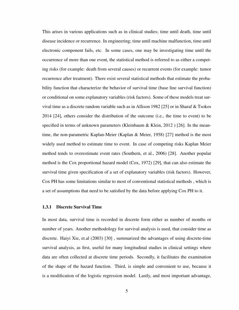
2.1.2 Recurrent (Recursive) Networks

Neurons in a Feedforward networks feeds only neurons of the next layers. Other types of

networks are formed such that neurons are feeding themselves or neurons of the preceding

layers or neurons of same layer, such networks are called recurrent networks. There are

several types of recurrent networks, such as the most two popular types are Hopfield neural

networks [35] and Bi-directional networks [36]. In some cases recurrent networks do not

have explicit definition of input and output layers(as in figure 3).

Figure 3.: Recurrent neural network, where doted lines represent indirect recurrences

Speech recognition and language learning are two of popular application of recurrent

networks [37–39]. Other important use of recurrent networks (Known as Real-Time Re-

current Networks) is in the modeling of time series data as we will show later in chapter

five. Figure 4 displays feedforward network with output going back as one of the inputs

which is used in modeling non-linear auto-regressive models.

In this dissertation we will see the utilization of feedforward neural network and re-

current neural networks (the one in Figure 4) in performing statistical modeling such as

survival analysis and time series analysis.

15

Figure 4.: Type of feedforward network with recurrent property. Either output is goingback as one of the inputs or the error.

2.2 Learning method of Neural Networks

Neural networks are inspired by the human nervous system making them learn in the same

way as human learns, which is by example. This type of learning is called supervised

learning, that is, neural network is given set of examples (data). Consider some data (X, t) ,

whereX is a matrix of information (covariates) and t is vector of targets, response variable,

that acts as a teacher forcing neural network to find the best approximated output to the

target values. Another type of learning for neural network is called unsupervised learning,

in which a network decide on its own what would be the best output fit for a set of data

without external help [40].

In this section we summarize the idea of training neural network from C. Bishop books

“Neural Network for Pattern Recognition” [41] and “Pattern Recognition and Machine

Learning” [34]. To train a neural network we need to estimate the weights that minimize

error function chosen for the certain task of the neural network. One of the most popular

algorithms to do so is called back-propagation, and it took this name as it is based on

propagating the errors backward from output neurons to neurons of first layer. For example,

consider similar structure of neural network as in Figure 1, that will be used in a linear

16

regression problem. We have data in the form of set of covariates and targets {Xs, ts} ,

where s = 1, 2, . . . , N number of observations. The network activation function for the

output unit in this case would be the linear (identity) function, and therefore the best choice

of error function E will be the mean square error given by:

E =1

2

N∑s=1

(y(xs, ω)− ts)2 (2.6)

where y(xs, ω) is the network output for observation s, which can be expressed in terms

of probability. For instance (In regression problem), if our target follows a Gaussian distri-

bution then network output can be expressed as:

p(t | x, ω) ≈ N (t | y(x, ω),1

β) (2.7)

where β is the inverse variance of the Gaussian (noise) distribution. From equation (2.7)

one can find the likelihood function for the whole N observations on the form {Xs, ts} as :

p(t | X, ω, β) = ΠNs=1p(ts | xs, ω, β) (2.8)

So one can estimate network weights ω by maximizing the negative logarithm of (2.8),

which in neural networks literature is equivalent to minimizing the error function in (2.6).

The most popular algorithm used in minimizing the error function is back-propagation that

consists mainly of two parts.

2.2.1 Evaluating derivatives of Error function

The first part of training neural networks through back-propagation is to evaluate the deriva-

tives of the error function with respect to the network weights.

To evaluate the derivatives we will introduce some notations first:

• The first function for a given neuron j as we explained earlier is the weighted sum given

17

by:

aj =∑i

ωjizi (2.9)

where ωji is the weight passing information from neuron i to neuron j . And, zi is the

output of neuron i of the preceding layer.

• The output of each neuron zi is computed by the activation function as:

zi = h(aj) (2.10)

where h() is the activation function (as mentioned earlier it can be ; identity function,

sigmoid or softmax).

• Recalling equation (2.6), the error function is a function of the network weights through

the summed inputs aj , so by applying the chain rule we obtain:

∂E

∂ωji=∂E

∂aj

∂aj∂ωji

(2.11)

By using (2.9) we obtain ∂aj∂ωji

= zj , then (2.11) is simplified to:

∂E

∂ωji= δjzj (2.12)

where δj is given by:

δj = h′(at)

∂E

∂yt(2.13)

for neurons in the output layer. Where t is number of neurons in output unit, and yt is

the output of neurons in the output layer. The neurons in hidden layers δj is given by:

δj = h′(at)

∑t

ωtj δt (2.14)

18

equation (2.14) represents the back-propagation formula as the error derivatives are

propagation backward from neurons of output layer to neurons of hidden layers.

Once the derivatives of (2.12) are calculated then it is the time to turn these derivatives

to learning rule to change network weights. Updating the weights can be done after each

observation (called on-line learning) or after all data have been passed through the network

(batch learning) by summing the derivatives over all observations N

∂E

ωji=

N∑s=1

∂Es∂ωji

(2.15)

2.2.2 Optimization Algorithm

The second part of training neural networks by the back-propagation algorithm is to use

the derivatives of the error function (2.12) and turn them to learning rule to adjust the net-

work weights. This is done by involving a non-linear optimization algorithm like gradient

descent or quasi-Newton method among others. We are going to discuss the quasi-Newton

method as it was the one used in training our neural networks in next chapter. Our goal

is to find weight vector ω that minimize the error function E (ω). Imagine this problem

graphically as error surface sitting on weight space, so we need to find the gradient of the

error in the weight space that will lead us to minimum point in the space (OE = 0). The

gradient of error using quasi-Newton method is given by:

graident = OE = H(w −w∗) (2.16)

where H is the hessian matrix that can be obtained by the second derivatives of the error

function with respect to the weights (H = ∂2E∂ωi∂ωj

). And, the weight vector w∗ satisfies

w∗ = w −H−1OE (2.17)

19

where H−1OE is known as Newton’s direction/step that automatically determines the size

and the direction of the step towards the error minimum. Since the direct calculation of

the Hessian matrix is computationally expensive (which is known by Newton’s method),

the alternative is by building up an approximation to the inverse Hessian over a number of

steps (which is known by quasi-Newton method) [41]. The approximation of the Hessian

matrix involves generating a matrix G(k) at step k as follows:

Gk+1 = G(k) +ppT

pTv− (G(k)v)vTG(k)

vTG(k)v+ (vTG(k)v)uuT (2.18)

where we define:

p = wk+1 −w(k) (2.19)

v = g(k+1) − g(k) (2.20)

g: is the gradient in (2.16). And,

u =p

pTv− G(k)v

vTG(k)v(2.21)

initial choice of G would be the identity matrix then we can replace Newton’s step−Hg in

(2.17) by −Gg. However, as Bishop [41] mentioned full Newton’s step in (2.17) may take

the search outside the approximation valid area and thus the use of line-search algorithm is

applied and (2.17) becomes:

wk+1 = w(k) + ζ(k)G(k)g(T) (2.22)

where ζ(k) is found by line minimization.

The draw back of quasi-Newton method is the need of more storage to update matrix

G as the number of network weights increases. Moreover, quasi-Newton method follows

20

always a descent direction in the space so it can be trapped in local minimum as going

out from that point requires increase in the error function which is not allowed. Neural

networks popular draw back in general is the excess time it may take to approximate func-

tion based on certain case not only because of the optimization algorithm used but also if

weights were allowed to take large values during training, which is similar to the perfor-

mance of human brains when large information are processed through it in a certain time.

In another words, If network weights are allowed to take on large values, conversion of the

optimization algorithm becomes slower. The solution for the previous issue is solved by

introducing additional term called weight decay α, that controls the variance of the weights

and penalize large weight values. Weight decay is based on Bayesian method that will be

discussed in the following section. The Error function for networks working with weight

decay becomes:

E = ED + αEW (2.23)

where ED is the error due to approximation of network outcomes to targets given by (2.6)

and

EW =1

2

W∑i=1

ω2i (2.24)

2.3 Bayesian Neural Networks

In this section we will discuss the use of Bayesian inference methods in neural networks.

David MacKay [42–44] proposed the use of Bayesian in neural network and after him,

R. Neal [45] updated his work, so more details can be found in their papers. The use of

Bayesian in neural networks have several advantages:

1. Helps in determining the optimal values for the regularization parameters (like weight

decay) by estimating them online from the training data.

2. Regularization can be given a natural interpretation in the Bayesian framework.

21

3. Parameter uncertainty can be accounted for in the network predictions and hence over-

fitting is not an issue.

4. Helps in comparing between several neural network architectures using training data

only.

5. The relative importance of input variables can be determined using automatic relevance

determination [45, 46]

In the previous section we talked about training neural network through the maximum

likelihood. In Bayesian setting we find the conditional probability of network outputs

through posterior distribution of the network weights. Through Bayesian inference the

posterior distribution of a vector of weights ω given a set of dataD (whereD contains both

set of variables information X and its corresponding targets t) is given by:

p(ω | D) =p(D | ω) p(ω)

p(D)(2.25)

where p(D | ω) is the data likelihood, p(ω) is the prior distribution of the weights, and p(D)

in the normalization factor (also called the evidence). So once the posterior distribution in

(2.25) is calculated then network prediction output for a given input x′ can be obtained by:

p(y | x′ ,D) =

∫p(y | x′ , ω)p(ω | D) (2.26)

as we know in Bayesian, the integral of (2.26) in most cases is analytically intractable and is

approximated or we use simulations to evaluate it. Two methods for evaluating the integral

of (2.26) will be discussed, the first is the evidence procedure [43] and the second uses the

Hybrid Monte Carlo [45]. Before we discuss the two methods we will talk first about the

choice of prior of the network weights.

22

2.3.1 Neural Network Weights: Choice of Priors

The choice of priors rises from the need of having small weights so we can obtain smooth

network performance and to avoid mapping with large curvature. This need for small

weights suggest a Gaussian prior with zero mean, given by:

p(ω) =1

ZW(α)exp

(−α

2

W∑i=1

ω2i

)(2.27)

where α in the inverse variance of the weight distribution and ZW(α) is the normalizing

constant given by:

ZW(α) =

(2π

α

)W2

(2.28)

after ignoring the normalizing constant of (2.27) and taking the negative log, we will find

that the prior is equivalent to the error term of (2.24). This error term regularizes the weights

by penalizing over large values. The weights distribution is assumed to be a Gaussian

distribution with mean zero and variance1

α, so the value of the hyperparameter α controls

the weights of fanning out from each input variable and hence large alpha values means

small variance so inputs are of less relevant to output. This approach can be generalized

by assuming different hyperparameters for each input variable. This procedure is known

as automatic relevance determination (ARD). In the following we will discuss the two

methods for evaluating the integral of (2.26)

2.3.2 The Evidence Procedure

The evidence procedure introduced by MacKay [43] as an iterative algorithm for determin-

ing optimal values for network weights and hyperparamters. It is not considered as fully

Bayesian as it searches for optimal values rather than integrating out the whole vector of

weights in (2.26). By introducing the hyperparameters, the posterior probability distribu-

23

tion of the network weights is given by:

p(ω | D) =

∫ ∫p(ω | α, β,D)p(α, β | D)d α dβ (2.29)

To evaluate the latter integral which is at least double integral and usually will be more (de-

pending on the number of different hyperparameters), The evidence procedure approximate

the latter integral to:

p(ω | D) ≈ p(ω | αMP , βMP ,D) (2.30)

whereαMP and βMP are the most probable values of the hyperparameters. These values are

considered to be the values where the posterior density of the hyperparameters is peaked

around. Which means that first we need to estimate the most probable hyperparameters,

then next step involves integrating the posterior distribution of the weights (2.30) to ob-

tain network outputs. So, first step in the evidence procedure is to evaluate the posterior

distribution of hyperparameters by approximating it to the most probable values of hyper-

parameters. Using Bayesian inference, the posterior distribution of the hyperparameters is

given by:

p(α, β | D) =p(D | α, β) p(α, β)

p(D)(2.31)

where p(D) can be ignored since in the evidence procedure we only need the peeks this

density. p(α, β) is the prior density of the hyperparameters in which there exist a wide

range of choices for the prior based on the applied problem we will be using the neural

network on. For the meantime we will assume uniform distribution as the prior of the

hyperparameters so it can be ignored in the rest of the analysis. This leave for us the

likelihood p(D | α, β) which we need to maximize by finding the peek values of α and β.

p(D | α, β) is also known as the evidence that can be used to compare between different

24

neural network structures. The evidence is given by:

p(D | α, β) =1

ZD(β)

1

ZW (α)

∫exp(−S(ω))dω (2.32)

and to find find the values of α and β we take partial derivative for the log of (2.32). In

the evidence procedure the Hessian matrix A of the error function S(ω) is evaluated at

A = H + αI (2.34), so by differentiating log of (2.32) with respect to α and equating to

zero we get:

αnew =γ

2EW(2.33)

where γ =∑W

i=1α

λi+α, so that λi + α are eigenvalues of A. Following same for β we

obtain:

βnew =N − γ2ED

(2.34)

Now it is turn to find the weights posterior distribution, recall the goal in Feedforward

networks is to find the set of weights that minimize the error function. MacKay used

another approximation for the error function (also known as the cost function) as a second

Taylor-expansion that have local minimum at ωMP . The expansion of error function S(ω)

is given by:

S(ω) ≈ S(ωMP) +1

2(ω − ωMP)TA(ω − ωMP) (2.35)

where A is the Hessian matrix of the total error function:

A = ∇∇S(ωMP) = βH + αI (2.36)

where H = ∇∇ED(ωMP), and since it is preferable that the error S(ω) to have Gaussian

distribution, it follows that the posterior distribution of (2.30) is:

p(ω | D) =1

ZSexp

(−S(ωMP )− 1

2(ω − ωMP )TA(ω − ωMP )

)(2.37)

25

where ZS is the normalizing factor of the Gaussian distribution for the error function.

Finally we can summarize the evidence procedure in the following algorithm:

1. Choose initial values for hyperparameters α and β, and network weights and bias.

2. Train neural network with appropriate optimization algorithm to minimize the error

function S(ω).

3. Then using the Gaussian approximation for the hyperparameters, new values of hyper-

parameters can be found using (2.33) and (2.34).

4. Repeat steps 2 and 3 until convergence is reached.

Note that evidence procedure can be implemented easily but choosing different initial α

values for each of the input variables.

2.3.3 Hybrid Monte Carlo Method for Neural Networks

The idea that Mackay presented for applying Bayesian inference in learning of neural net-

work was improved by Neal [45]. The origin of hybrid Monte Carlo sampling returns to

Duane [47]. Neal enhanced Bayesian neural networks by calculating the integral of (2.26)

using Hybrid Monte Carlo sampling, to sample from the weights posterior distribution. In

Hybrid Monte Carlo method the integral in (2.26) is approximated by:

p(y | x,D) ' 1

N

C∑c=1

p(y | x,ωc) (2.38)

where {ωc} represent a sample generated from the posterior distribution of the weights.

The hybrid Monte Carlo combines stochastic sampling techniques with the Metropolis-

Hastings algorithm. Since in neural network we can easily evaluate the gradient informa-

tion using the back-propagation technique, this gradient information can be used to direct

the direction of MH algorithm. Though Neal have shown that his approach is better than

26

using the evidence procedure but still have some back flaws. First, Neal uses initial val-

ues for the hyperparameters that does not change with respect to the data, and as it is well

known that the Bayesian prediction is as good as the choice of the prior. Unless we are sure

about the priors belief, using the Hybrid Monte Carlo sampling by Neal will require a huge

number of trails to test for different values of hyperparameters. Secondly, it is highly timely

consuming method, especially with today’s massive data used to predict certain problem.

In Chapter four we shall introduce a solution for the latter problem by applying a mixture

of the evidence procedure and the Hybrid Monte Carlo sampling. Furthermore, we are

going to show in chapter four that we did not only obtain the lowest error by using this

new approach, but we also were able to obtain neural network models in much shorter

computational time.

27

Chapter 3

Prediction of Survival Time for Melanoma Patients Using Artificial Neural Network

In Chapter 1, we mentioned several models that were introduced to model survival time

using artificial neural networks. However, in literature we did not see any comparisons

among these models. In this chapter a comparison between two of these methods that

utilize artificial neural network in predicting survival time is performed.The first method is

called the partial logistic artificial neural network (PLANN), [10], and the second method

we call it discrete hazard artificial neural network (DHANN), [12]. The comparison is done

using real world data on skin cancer patient specifically malignant melanoma, the most

deadly type of skin cancer. Also, we study the difference between the survival time of male

and female melanoma patients.

3.1 Melanoma Patient Data

In the present study we use 130,006 patients diagnosed with melanoma between the years

2000 to 2009 in the US. Data accumulated from 13 registers of the Surveillance, Epidemi-

ology, and end results program (SEER) [48]. We filter out this large data set to contain

only consummate information with respect to the patient’s age at diagnosis, tumor thick-

ness, stage of cancer and ulceration. Soong et al. [4] in 2010 used these four variables, but

their study did not consider the difference between male and female survivals. We found

that there exists a significant difference between the median survival time of males and

females based on a 5% level of significance using the Kruskal-Wallis test. Thus, studying

the effect of gender on survival time by making one model for both males and females is

28

not statistically correct, as the survival time for male and females does not have the same

probability distribution. Figure 5, below, represents a schematic diagram of the distribu-

tion of the complete data with respect to gender and cancer stage. We train neural network

model separately for males and females.

Total

69082

Males

39147

Stage 0

953

Stage 1

32980

Stage 2

4370

Stage 3

844

Females

29935

Stage 0

751

Stage 1

26093

Stage 2

2679

Stage 3

412

Figure 5.: Distribution of complete information of melanoma patients

Figure 5, also includes the total number of patients with complete information who were

diagnosed with melanoma between the years 2000 to 2009. Patients were either alive at

the end of the 10 year period (censored) or lost follow up during the ten year interval (cen-

sored). In addition, patients who died because of melanoma (uncensored) and percentage

of censored patients split as 95% of male patients were censored and 98.1% of female

patients were censored. We omitted patients with incomplete information. For training

purposes, each of the gender category data was divided into six groups; five will be used

in the cross validation technique to train and validate the neural network model, while the

last group is used for prediction and accomplishing the comparison between the two mod-

eling approaches. More details about the cross validation will follow in the next section. In

our modeling procedure, we used age at diagnosis and tumor thickness (in millimeter) as

29

quantitative variables along with three dummy variables representing stage 1 (referring to a

localized tumor), stage 2 (referring to a regional tumor), and stage 3 (referring to a distant

tumor). The base level is referred to as in situ tumor.

3.2 Methodology

In this section we are going to discuss the two method PLANN and DHANN. Both of the

two methods used three layer Feedforward neural network.

3.2.1 Partial Logistic Artificial Neural Network (PLANN)

Partial logistic artificial neural network (PLANN) is the approach that was introduced by E.

Biganzoli et. al. [10]. PLANN is a three layer feed forward artificial neural network with

one output unit in the output layer. The activation function used in the hidden and output

layer is the sigmoid (logistic) function given by (2.2). PLANN estimates the conditional

hazard function that is based on the discrete survival method (discussed in chapter one).

Recall that the discrete hazard probability function for time period k given a vector of

covariates xi is given by

hk(xi, tk) =1

1 + exp(−αktk − βtxi)(3.1)

where tk represents the time input for time period k. To estimate the conditional hazard

in (3.1), PLANN uses three layer Feedforward network with an activation function for the

hidden and output layers given by (2.1). The output of the network with an H number of

hidden units is given by:

h(xi, tk) = f

[b+

H∑h=1

ωh f(ah +P∑p=1

ωphxip)

](3.2)

30

where ωph and ωh are the weights of the ANN to be estimated for the first layer and second

layer respectively, also ah and b are the weights for the bias connection with the hidden units

and with the output unit respectively. The target of this network is the censoring indicator

cik, which takes the value one if the event occurred for subject i, and zero otherwise. The

cost function used in PLANN is the cross-entropy function which is appropriate for binary

classification problems, [41]. The weights of PLANN can be estimated by minimizing the

cost function given by

E = −n∑i=1

ki∑k=1

{cik log

[h(xi, tk)

]+ (1− cik) log

[1− h(xi, tk)

]}(3.3)

Once the network weights are estimated, the monotone survival probabilities can be easily

found by converting the discrete hazard rate estimates obtained from the network output by

using the following equation:

S(tk) =k∏l=1

{1− h(tl)} (3.4)

The advantage of this approach is that the time dependent covariates can easily be intro-

duced in the model, as the individual records are available for each time period. However,

for large data sets or studies conducted over a long period of time this approach is inac-

cessible due to the immense number of replication requisites, [49]. Figure 6 on next page,

shows the architecture of the PLANN introduced by Biganzoli. The first layer contains the

bias and one node for the time period and the rest of the nodes for the covariates. PLANN

uses one input for the time to estimate smooth discrete hazard rates. However, we have

used 10 nodes for the time (one for each time period) to be able to compare it with the

second method (DHANN).

31

bias

HIDDENINPUT

Covariates

bias

OUTPUT

Conditional hazard probability

Figure 6.: Feedforward ANN for partial logistic artificial neural network, with three layers.The input layer has p covariates and hidden layer with H hidden units and one output unitin the output layer. Activation function used in both hidden and output layer is the logisticfunction (2.1).

3.2.2 Discrete Hazard Artificial Neural Network

Mani [12] developed an approach that predicts the hazard discrete function similar to an

approach by Street [50], that predicts the survival function using a neural network with K

outputs, where K is the number of time periods. He trained his network utilizing a target

vector derived by Kaplan-Meier survival curves [51]. Mani used same neural architecture

as Street, but rather estimate the hazard function not the survival function. In order to

estimate the hazard function, each individual or subject would have a training vector (1 by

K) target of hazard probabilities hik as follows:

hik =

0 for 1 ≤ k ≤ K

1 for t ≤ k ≤ Kand event = 1

rknk

for t ≤ k ≤ Kand event = 0

32

here, hik = 0 for each time period patient i survived. hik = 1 from time interval t to K

if patient died because of melanoma at duration t within the study time. And, for those

patients who lost follow up during the study of duration t < K their hazards are equal to

the ratio rknk

, which is the Kaplan-Meier hazard estimate for time interval k. Also, rk is the

number of patients who died because of melanoma in time period k , and nk is the number

of patients that are at risk in time interval k. For training the neural network, Mani used the

logistic sigmoid function given by (2.1). The network weights are estimated by minimizing

the cost function, which is the cross entropy function. Figure 7, shows the neural network

architecture utilized by DHANN. The number of units p of the input layer are equivalent

to the number of independent variables or risk factors. The K output units of the output

layer learns to estimate the hazard probability of each individual. Once the ANN is trained

and the hazard estimates are predicted, we convert those hazard estimates to the survival

estimates by using (3.4), for each method. We have trained the weights of the ANN for

both methods using the quasi-newton algorithm discussed in chapter 2.

bias

HIDDENINPUT

Covariates

bias

OUTPUT

ℎ𝑖1

ℎ𝑖2

ℎ𝑖𝐾

Figure 7.: DHANN: Three layer network with K output units in the output layer whereK is equal to the number of time intervals.

33

3.3 Model Selection

Now, we are concerned in identifying the optimal number of hidden units in the hidden

layer that will give us the best neural network model. There are several methods in literature

that we can use to select the best neural network. The most popular method is the v-fold

cross validation method as it does not rely on any probabilistic assumptions and help in

determining when over fitting occurs. Other statistical methods like hypothesis testing or

information criteria that were introduced and examined by Ulrich Anders and Olaf Korn in

1999, [52] for neural network model selection, they suggested that these statistical methods

should take part during the process of developing neural network models. However, since

their proposed methods were based on certain probabilistic assumptions, it may not be

always applicable in modeling real phenomena. In order to do our comparison we took

the best neural network for each method and then tested their performance using the same

set of data, this set of data was not used in the training process to identify the model. In

the current study, we have used 5-fold cross validation to select the best model for each

method, PLANN & DHANN. We divide the male and female data sets into six groups.

Five were used in the training and validation, and the last group was used for comparing

the best models from the two methods together (hold out data set). In addition, we use the

weight decay that helps avoid over fitting and penalize large weight solutions to help in

generalization.

As mentioned by B. Ripley [53, 54] a weight decay value between α = 0.01 and α =

0.1 would be more appropriate depending on the degree of fit that is expected. We have

used the cross validation method along with four different values of weight decay α =

{0.025, 0.05, 0.075, 0.1}, to pick the best model.The same procedure of trying different

weight decay values were used in, [10]. The cross validation method will help us in finding

the optimal number of hidden nodes. In addition, we consider the model with the lowest

prediction error when applied to a new data set. Therefore, for each method we picked

34

the best model, with lowest cross validation error, then compare their performance on the

hold out data set. We repeated our comparison for the four values of weight decay, since

for same data two factors affects ANN performance (Number of hidden units and Weight

decay value).

3.4 Results

In our analysis, we used ten time intervals (12 month each) and in order to do the compari-

son between the PLANN and DHANN method we used 10 inputs for the ten time intervals

in PLANN instead of one, so that we can compare the output of the PLANN with the sec-

ond method. After training, the cross validation method resulted in choosing the networks

with 52 hidden units (number of hidden nodes seems to be large but by taking into account

the number of output units, we have 10 parallel networks with five hidden nodes each)

for both methods as the best model. We obtain similar results from ANN trained with the

four different values of weight decay. Still, we want to examine the prediction accuracy

for all eight available models to choose our best-fit model. Table 1 shows the comparison

between the eight models for male melanoma patients and Table 2 shows the comparison

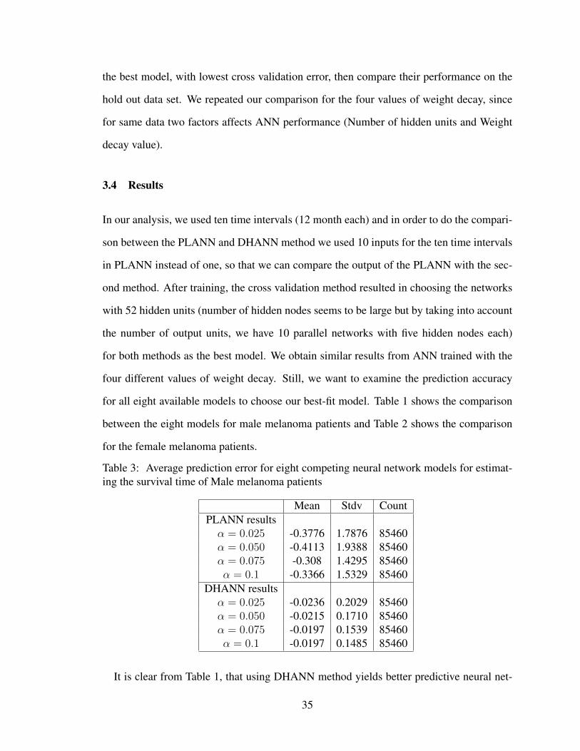
for the female melanoma patients.

Table 3: Average prediction error for eight competing neural network models for estimat-ing the survival time of Male melanoma patients

Mean Stdv CountPLANN resultsα = 0.025 -0.3776 1.7876 85460α = 0.050 -0.4113 1.9388 85460α = 0.075 -0.308 1.4295 85460α = 0.1 -0.3366 1.5329 85460

DHANN resultsα = 0.025 -0.0236 0.2029 85460α = 0.050 -0.0215 0.1710 85460α = 0.075 -0.0197 0.1539 85460α = 0.1 -0.0197 0.1485 85460

It is clear from Table 1, that using DHANN method yields better predictive neural net-

35

work model than the PLANN . Among the four competing models of DHANN method

we have chosen the model with weight decay α = 0.1 as the best fit model for predicting

survival times of male melanoma patients, that yield smaller mean error and standard devi-

ation. While the results in table 2 supports the decision we have made for male melanoma

patients that DHANN method has a better predictive accuracy than that of the PLANN.

But the best model for predicting the female melanoma patient’s survival time is the model

with weight decay value α = 0.075.

Table 4: Average prediction error for eight competing neural network models for estimat-ing the survival time of Female melanoma patients

Mean Stdv CountPLANN resultsα = 0.025 -0.3384 2.1326 69130α = 0.050 -0.2274 1.4451 69130α = 0.075 -0.1882 1.1672 69130α = 0.1 -0.2011 1.2199 69130

DHANN resultsα = 0.025 -0.0208 0.2310 69130α = 0.050 -0.0183 0.1849 69130α = 0.075 -0.0167 0.1606 69130α = 0.1 -0.0246 0.3022 69130

3.5 Survival Time Findings

It is clear to us that male and female melanoma patients need to be treated differently

as its shown by the survival plots in figure 8, which displays the surface plot of survival

probability of male (plot on the left) and female (plot on the right). In figure 8, the survival

is estimated as a function of Age at diagnosis and time in years. The tumor thickness is

0.58 mm and ulceration variable is set to 0 and considering the patient was diagnosed in

the initial stage. Male infant patients have less survival probability than that of female

infant patients over a 10 year period. Where as a male patient at age 40 to 50 seems to

have higher survival probabilities compared to female patients at the same age. Figure 9,

36

Figure 8.: Survival probability function surface plot results for Age for male melanomapatients. Plot on left for male patient. Plot on right for female patient

Figure 9.: Survival probability function surface plot results for tumor thickness. Plot onleft is for the male patient diagnosed at age of 20 years old. Plot on right for male diagnosedat age 60 years old.

37

Figure 10.: Survival probability function surface plot results for tumor thickness. Plot onleft is for the female patient diagnosed at age of 20 years old. Plot on right for femalediagnosed at age 60 years old

displays the surface plot of survival results for male melanoma patients for tumor thickness

ranging from 0.01 mm to 9 mm. The surface plot (on left) is for male patient diagnosed

at 20 years of age, whereas the plot (on right) for male patient diagnosed at 60 years old.

As we can see survival estimates for young men is farther away and lower than that of

older men, these findings were found similar to a recent study by D. Fisher and A. Geller

in 2013 [55]. Fisher and Geller mentioned that more attention was given to older men over

the past years and suggested that more awareness needed to be addressed to young men to

help in early detection of melanoma. They also mentioned the difference between young

men and young women, which we can figure out by comparing the two left plots of figure

9 and figure 10. The survival probability for young men (diagnosed with tumor thickness

larger than 4mm) within two years of diagnosis is too low (almost 0) compared to that of

young women. Some of our significant findings were found to be similar to those found in

another study by C. Gamba et. al. in 2013 [56]. However, more investigation and statistical

data analysis are required to better understand the causes of the differences between young

males and females, and to plan new strategies to fight the major pernicious form of skin

38

cancer (melanoma).

3.6 Conclusions

In modeling survival data with artificial neural network, it is more prevalent to utilize

DHANN. The prediction accuracy is much better compared to the PLANN. However, the

results may change if some how the survival data contains time varying covariates (risk

factors). One can attempt to amend the PLANN model by differentiating between the in-

dividuals who survived the whole duration time and those who dropped out during the

duration time, which opens another area of research in this field. With regard to learning

techniques for ANN, P. J. Lisboa [57] have amended the PLANN by adapting the Bayesian

learning for neural networks, developed by Mackay in 1995 [44]. It is still an open problem,

How the Bayesian learning will affect the performance of DHANN? Whether it’s going to

change the comparison results with the PLANN?, among other questions that we need an-

swers and opens more areas of research on this type of problems. Some of the contributions

we obtained from the current study is:

1. The use of artificial neural network have priority over conventional statistical methods,

which is being able to form a model with several response variables.

2. There exist two strong methods for predicting survival time using artificial neural net-

work. If data used consists of time varying covariaties (Use PLANN). If data does not

contain time varying covariates (Use DHANN).

3. The current study opened the door to additional research points, one of which, How to

use DHANN in the analysis of competing risks?

In chapter 4, we present a solution for using DHANN in the analysis of competing risks,

by introducing binary variables for each risk in the matrix of covariates.

39

Chapter 4

New Bayesian Learning for Artificial Neural Networks with Application on Survival

time for Competing Risks

In the present chapter, we introduce a new method of utilizing artificial neural network

(ANN) in modeling survival data of competing risks. Additionally, we present and validate

a new Bayesian learning technique for neural networks. The new neural network archi-

tecture that we propose in this chapter is used to study the risks associated with patients

diagnosed with melanoma (skin cancer). Patient’s information diagnosed with melanoma

in the United States from the years 2000 to 2010 were gathered from the Surveillance, Epi-

demiology, and End Results Program (SEER) [58]. We used Harrells c-index to validate

the new proposed neural network structure, in addition we used the v-flod cross validation

method to check the model on different set of data and to find the best fit number of hidden

units.

4.1 Literature Review

In chapter 1 we reviewed several methods used for survival time analysis. Another set of

models that arises and uses artificial neural networks (ANN), two of which we discussed

in chapter 3. ANN is well known in clinical trials as a predictor classifier, predicting the

diagnosis of a specific cancer as in (Khan, et al., 2001), among several others. In survival

analysis, ANN was previously used to predict whether a patient will live the current time

period or not (Bottaci, et al., 1997) [6], others were proven to be better than the Cox PH

model (Taktak, et al., 2007) such as the partial logistic artificial neural network PLANN

40

[10]. In which the authors presented a method by utilizing ANN to model survival time as a

function of other variables using the partial logistic regression approach on censored data as

we discussed on previous chapter, also an extension of PLANN for competing risks analysis

PLANNCR, by Bignazoli, Boracchi, Ambrogi, & Marubini, 2006,[59]. PLANNCR is

a neural network, that shares same input layer structure as PLANN where time interval

is treated as ordinal variable and activation function use in hidden layers is the logistic

function, similar to PLANN. The output layer in PLANNCR consists of a number of output

units equal to the number of risks in the study. The activation function for output unit r is

the softmax function given by

htr =Ztr(x)∑R+1

r=1 exp [Ztr(x)](4.1)

where Ztr(x) is the function of predictors. Beside the choice of the Kullback-Leibler

distance as the error function makes the PLANNCR perform as a generalized linear mod-

els. PLANNCR predicts the conditional probability that a subject will be censored in the

tth time period for the R risk, and by comparing it to other competing models used for

competing risks, the PLANNCR came the best. But still as we clarified in chapter 3 that

due to the use of time as one of network inputs makes you repeat subjects information. We

have shown that this was one of the reasons why DHANN performed better than PLANN

in a single risk case. One of our goals in this chapter is to amend the DHANN to be able to

model survival functions for competing risks.

On the other hand, training of ANN should be done with cautions, as over-fitting is a

major problem in any ANN system. That is, error of unseen data set (different from the

data set ANN was trained on) occurs to be larger than the training error. The use of a

penalty term based on Bayesian method was introduced to over come over-fitting issues

(Bishop, 1995) [41], and it was used in PLANN and PLANNCR. However, the learning of

PLANNCR was further improved by applying the Bayesian regularization (known as the

evidence procedure) for training neural networks (MacKay, 1992)[43] by (Lisboa, et al.,

41

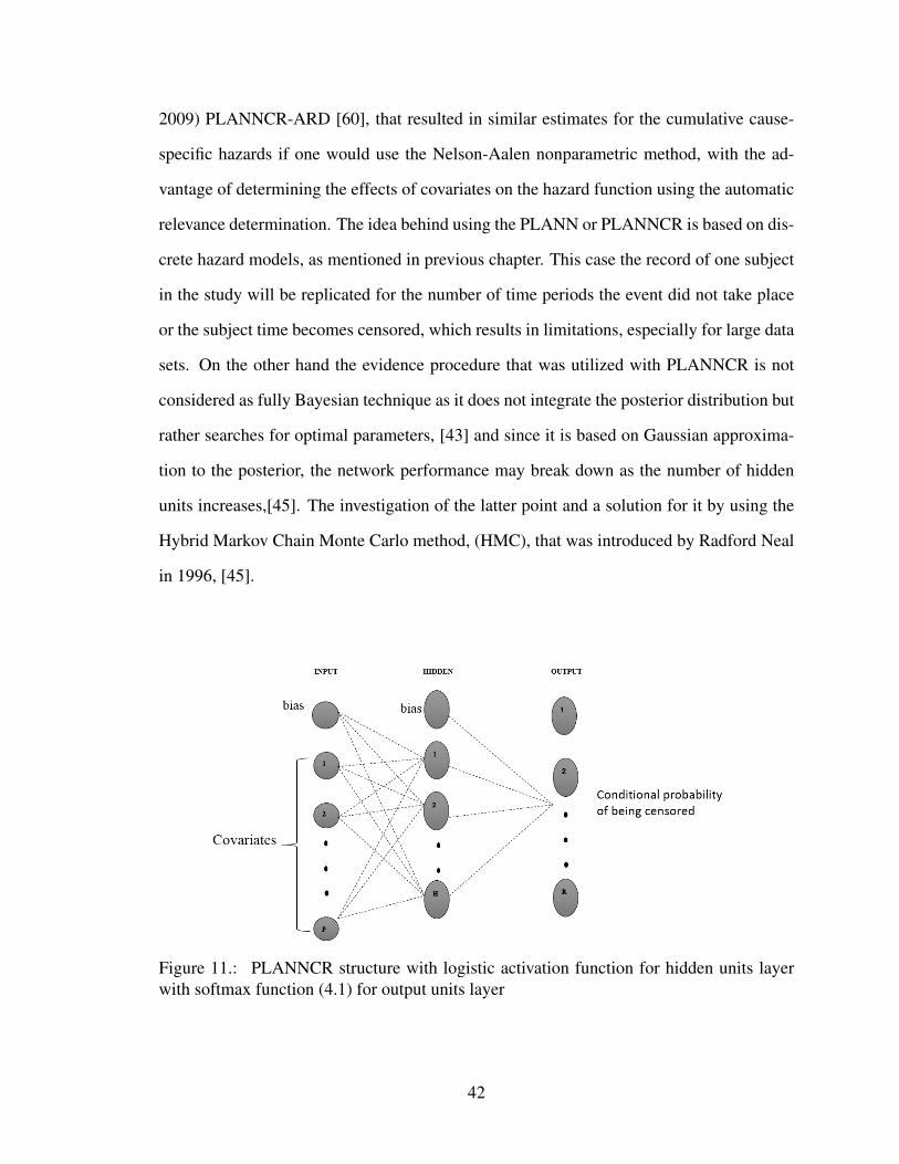
2009) PLANNCR-ARD [60], that resulted in similar estimates for the cumulative cause-

specific hazards if one would use the Nelson-Aalen nonparametric method, with the ad-

vantage of determining the effects of covariates on the hazard function using the automatic

relevance determination. The idea behind using the PLANN or PLANNCR is based on dis-

crete hazard models, as mentioned in previous chapter. This case the record of one subject

in the study will be replicated for the number of time periods the event did not take place

or the subject time becomes censored, which results in limitations, especially for large data

sets. On the other hand the evidence procedure that was utilized with PLANNCR is not

considered as fully Bayesian technique as it does not integrate the posterior distribution but

rather searches for optimal parameters, [43] and since it is based on Gaussian approxima-

tion to the posterior, the network performance may break down as the number of hidden

units increases,[45]. The investigation of the latter point and a solution for it by using the

Hybrid Markov Chain Monte Carlo method, (HMC), that was introduced by Radford Neal

in 1996, [45].

Figure 11.: PLANNCR structure with logistic activation function for hidden units layerwith softmax function (4.1) for output units layer

42

4.2 Melanoma Patient’s Data

Data used in validating our new proposed neural network structure for competing risks,

were collected from the Surveillance, Epidemiology, and End Results Program (SEER),

[58]. Data consists of patients diagnosed with melanoma in the United States from the

years 2000 to 2011, thus the period of study is eleven years. Since we are going to estimate

hazard function based on discrete survival method, we chosen to divide the study time

to eleven time intervals, each interval consisting of 12 months. We have chosen a total

number of patients with complete information of the risk factors used equal to 185,108. As

we did in our previous study, we divided our data set according to gender as they do not

share same survival time distribution. Figure 12 displays the number of patients divided by

Figure 12.: Distribution of Number of Patients with respect to Gender, Tumor behaviorand Stage of cancer

gender, then by tumor behavior, then cancer stage. As we can see, 97.5% of patients (Males

and Females) are diagnosed with invasive tumor behavior, known as Malignant. Although

skin cancer is curable, especially in early stages, it is also known to be deadly especially

43

with an invasive tumor behavior. So, the need of a model than can predict the survival time

of melanoma patients based on such variable (tumor behavior) is very important. The use

of such models that describes the behavior of risk factors on survival time is vital, to help

patients decide their course of treatment, and to be able to educate people on the importance

of checking up and give good care for their skin changes. A full list of selected risk factors

from SEER database is

• Age : Age of Patient at diagnosis by melanoma.

• Tu : Size of Tumor thickness diagnosed.

• Stage 1: Localized: An invasive neoplasm confined entirely to the organ of origin.

Stage 0: noninvasive is the baseline.

• Stage 2: Regional: A neoplasm that has extended either beyond the limits of the organ

of origin or onto regional lymph nodes or combination of both.

• Stage 3: Distant: A neoplasm that has spread to parts of the body away from the

primary tumor.

• Stage 4: Un-staged: Information is not sufficient to assign a stage.

• Behav: Identifies the tumor behavior either noninvasive (in situ) or invasive (malig-

nant).

• Seq: Sequence number, describes the number and sequence of all reportable malig-

nant, in situ, benign, and borderline primary tumors, which occur over the lifetime of a

patient.

For melanoma patients diagnosed in the United States between the years 2000 to 2011,

we have identified three possible risks; the first risk patient deceased by Melanoma, the

second risk patient deceased by a different Cancer, and the third risk patient deceased by

Non-Cancer. All of these risks were identified from the Cause of death variable in the

44

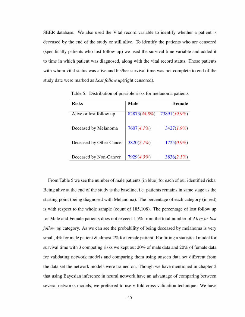
SEER database. We also used the Vital record variable to identify whether a patient is

deceased by the end of the study or still alive. To identify the patients who are censored

(specifically patients who lost follow up) we used the survival time variable and added it

to time in which patient was diagnosed, along with the vital record status. Those patients

with whom vital status was alive and his/her survival time was not complete to end of the

study date were marked as Lost follow up(right censored).

Table 5: Distribution of possible risks for melanoma patients

Risks Male Female

Alive or lost follow up 82873(44.8%) 73891(39.9%)

Deceased by Melanoma 7607(4.1%) 3427(1.9%)

Deceased by Other Cancer 3820(2.1%) 1725(0.9%)

Deceased by Non-Cancer 7929(4.3%) 3836(2.1%)

From Table 5 we see the number of male patients (in blue) for each of our identified risks.

Being alive at the end of the study is the baseline, i.e. patients remains in same stage as the

starting point (being diagnosed with Melanoma). The percentage of each category (in red)

is with respect to the whole sample (count of 185,108). The percentage of lost follow up

for Male and Female patients does not exceed 1.5% from the total number of Alive or lost

follow up category. As we can see the probability of being deceased by melanoma is very

small, 4% for male patient & almost 2% for female patient. For fitting a statistical model for

survival time with 3 competing risks we kept out 20% of male data and 20% of female data

for validating network models and comparing them using unseen data set different from

the data set the network models were trained on. Though we have mentioned in chapter 2

that using Bayesian inference in neural network have an advantage of comparing between

several networks models, we preferred to use v-fold cross validation technique. We have

45

chosen to split our data set to 10 approximately equally sized groups. More on the use of

v-fold cross validation will be explained in the Results section of this Chapter.

4.3 Discrete Hazard Artificial Neural Network for Competing Risks

In this section we present a new neural network model for predicting survival time of com-

peting risks. We will use the data discussed in the previous section to test and validate

the new proposed model. As we showed in Chapter 3, that the DHANN performed better

compared to PLANN. So, the new proposed neural network is an update to the DHANN

of single risk. The idea starts from Cox-PH for competing risks or what is known by the

Cox model for the cause-specific hazard [61], in which the conditional hazard for risk R is

given by:

hr[ t,X(t) ] = hor(t) exp[Z(t)′βr] (4.2)

where, Z(t) is a vector of p derived covariates, and hor is the baseline hazards. r =

1, 2, .., R number of risks. The aim of DHANN is to predict the discrete hazard proba-

bility for all time intervals at the same time by having the number of output units in the

output layer equal to the number of time intervals. It would be difficult to update DHANN

for competing risks, to follow PLANNCR approach which is training network to predict

the conditional probability of being censored for each risk (by having number of output

units in output layer equal to number of risks). So it means that if we consider that we have

3 possible risks, and our time intervals of the study is equal to 10, Then we need 30 output

units in the output layer, which is not practical. Our proposed solution for have DHANN

accommodate for competing risks is to add a number of binary variables equal to the num-

ber of required risks to the vector of derived covariates. In our case we have 3 possible

risks, so our derived vector of covariates Z(t) is given by

Z(t) = β01R1 + β02R2 + β03R3 + βX (4.3)

46

where (β01, β02, β03) presents the coefficients for the three binary variables R1, R2, and R3

respectively. The binary variables are defined as:

Rr =

0 for patient deceased of another risk or still alive

1 for patient deceased of the r risk

as we discussed previously, we are going to add three binary variables (meaning adding

also 3 additional input units in the neural network input layer) to the vector of risk factors

(covariates). The coding of these three variables is illustrated in the following table.

A patient that was deceased by melanoma, his/her record/row of information will be

starting with three additional values [1 0 0 · · · · · · ]. If a patient was deceased by other type

of cancer rather than melanoma (and is a melanoma patient), then his/her record will start

with [0 1 0 · · · · · · ]. If a patient was deceased by a non-cancer cause such as car accident,

heart attack, flu,etc. then his/her record starts as [0 0 1 · · · · · · ]. The last case would be

for patient who is still alive at the end of the study or lost follow and his/her vital status is

unknown or not known to be deceased, then his/her record starts as [0 0 0 · · · · · · ].

Table 6: Coding of the three added binary variables representing the possible risks

R1 R2 R3 Status

1 0 0 Deceased by Melanoma

0 1 0 Deceased by Other Cancers

0 0 1 Deceased by Non-Cancer

0 0 0 Still Alive or lost follow up

As we showed in Chapter 3, using DHANN requires the formation of training vector in-

stead of having one response variable. In case of DHANN the training vector was formed

with length (1 ∗ T ) , where T is the number of time intervals on the following form:

47

hik =

0 for 1 ≤ k ≤ K

1 for t ≤ k ≤ Kand event = 1

rknk

for t ≤ k ≤ Kand event = 0

Now we are upgrading the DHANN to fit competing risk model based on the addition we

did on the input layer. The training vector for the new method DHANN-CR is given by:

hi(t) =

0 event did not occur,

1 event took place in time t,

drjnj

if the subject is censored

(4.4)

wheredrjnj

is the Kaplan-Meier estimate of hazard probability for risk r. In the following we

will take an example of three patients to illustrate the reformation of data prior to applying

it to the DHANN-CR. Consider data of 3 patients are given in the following table

Table 7: Example of three patient records from SEER database

ID ST Age Tu S1 S2 S3 S4 Behav Seq Status1 109 51 1.25 1 0 0 0 1 2 Melanoma

2 130 35 0.85 0 0 0 0 1 1 Still Alive

3 96 63 1.01 0 1 0 0 1 2 Lost follow up

In Table 7, we have three patient record with the chosen 11 risk factors we identified

in the data section. Variables S1, S2, S3 and S4 stands for the the four different cancer

stages. Now, first patient was diagnosed by melanoma at Age 51, with tumor thickness

of 1.25mm, this patient have survived for 109 months (ST = 109). The status of the first

patient mentions that he/she deceased by melanoma. Then this patient record will start with

[1 0 0 51...] and his/her training hazard vector corresponding to his risk factors would be

48

[0 0 0 ... 1 1], in which for the first 4 time intervals the event did not take place and it

took place on the fifth year (i.e 5th time interval). Second patient record with start with

three binary values as zeros since patient is still alive at the end of the study and his/her

vector of training will be all zeros as neither of the expected 3 events took place (which

are deceased by melanoma, or deceased by another cancer, or deceased by a non-cancer

cause). In the meantime, the third patient lost follow-up from what appears in his/her

record of information. By looking at the third patient survival time (ST = 96) we obtain

that the patient lost follow-up after year eight, which means the eight’s interval, then the

training vector of this patient will start with zeros up to the eight time interval then for the

ninth, tenth, and eleventh values will be equal todrjnj

and since patient who lost follow-

up we repeat his record three times as he/she is in a risk of possible three events. The

reformation of the those 3 patients is illustrated in the following table by showing the first

3 values in patient record and his/her corresponding training vector.

Table 8: Example of Re-structuring data for DHANN-CR

ID Covariates training vectorR1 R2 R3 X1 ... Xp h1 h2 ... h9 h10 h11

1 1 0 0 x11 ... x1p 0 0 ... 0 1 1

2 0 0 0 x21 ... x2p 0 0 ... 0 0 0

3 1 0 0 x31 ... x3p 0 0 ... 0.0476 0.0498 0.02923 0 1 0 x31 ... x3p 0 0 ... 0.5331 0.0564 0.03213 0 0 1 x31 ... x3p 0 0 ... 0.1115 0.1248 0.0689

Once the data is re-structured the same way we explained in the previous example, we

can use the same neural network structure for hidden and output layers as in DHANN.

Figure 13, displays the new structure of DHANN-CR with our three identified risks.

4.4 New Bayesian Learning Technique

In Chapter 2, we explained the two Bayesian techniques used in learning of neural network.

Most of the application that have been using Bayesian learning were developed using the

49

Figure 13.: Structure of DHANN-CR with 3 identified risks

evidence procedure. Our aim is to be able to use the fully Bayesian learning technique

done through the hybrid Monte Carlo sampling(HMC). We propose a solution for the prob-

lems found in the HMC technique making researchers to avoid using it. As we mentioned

the HMC technique uses initial constant values for hyperparameters that does not change

based on the data. So, if the choice of initial hyperparameters does not capture the actual

prior belief, then neural network performance will not be good. A solution for the current

problem is use the part of re-estimating the hyperparameters of the evidence procedure as it

is done based on the data. Our approach is to reach an approximate values of hyperparam-

eters which capture the true distribution of weights variance. We called this new approach

(E-HMC), E: stands for evidence and HMC: stands for hybrid Monte Carlo sampling. Our

new proposed method (E-HMC) works as follows:

1. Choose initial values for hyperparameters α and β, and network weights and bias.

2. Estimate the most probable values of α and β that maximize the evidence given by

(2.32) considering the initial weight values as the most probable weight values, where

these values are estimated by using (2.33) and (2.34).

50

3. Use the HMC to sample from the posterior distribution of the weights, with hyperpa-

rameters value found in step 2.

To validate our proposed method, we trained our neural network models for the chosen data

set of melanoma patients using the three Bayesian techniques, the evidence procedure, the

HMC sampling method and the E-HMC,the newly proposed method. All neural networks

were trained with initial values of hyperparameters equal to 0.01. The automatic relevance

determination was also used to determine which of our 11 risk factors contributes more

towards the survival time of a melanoma patient. All neural networks models were trained

using MATLAB software, by using a set of algorithms done by Ian Nabney [62] called

NETLAB. The evidence procedure and the HMC sampling were the two major algorithms

we use from NETLAB, although we had to update some of the codes as it was done on

older versions of MATLAB.

4.5 Results

The main problem in statistical modeling is to find the model that best fits the data based

on two criteria; the first one with respect to the best neural network, mainly the number

of hidden nodes in hidden layers, and the second with respect to the learning algorithm.

In order to accomplish that we use two model validation techniques, the v-fold cross vali-

dation and Harrell’s C-indexv[63]. Harrell’s C-index, discrimination index, measures the

predictive accuracy of statistical models, and widely used in survival analysis to compare

the effectiveness between models. In 2005, there was an upgrade on the Harrell C-index to

get a time-dependent discrimination index for censored survival data by Antolini, Boracchi,

and Biganzoli [64]. Harrell’s C-index for proportional hazard models is given by:

c =

∑n−1i=1

∑nj=1;j 6=i concordanceij∑n−1

i=1

∑nj=1;j 6=i comparableij

(4.5)

51

where comparableij is the number of comparable pairs {i, j} from sample of n observa-

tions. And, concordanceij is the number of concordant pairs. The two variables represents

binary indicators that are defined as:

comparableij = I{STi < STj & di = 1}+ I{STi = STj & di = 1 & dj = 0} (4.6)

and,

concordanceij = I{z(xi) > z(xj)} ∗ comparableij (4.7)

where z(xi) is the linear predictor function in (4.2). We have created and implemented a

new algorithm in MATLAB to calculate the C-index for any neural network in the form of

PLANN, or DHANN, or DHANN-CR.

4.5.1 Algorithm for computing C-index through MATLAB

To find C-index we first find the number of comparable pairs then use it to calculate the

number of concordant pairs. Recall that we used 10-fold cross validation, so for the same

number of hidden units we have a total of 10 different neural networks models (Only in case

of using evidence procedure). Thus, the C-index is calculated for each of these networks

and then average it for the same number of hidden units for each time interval (we have a

total of 11 time intervals). The code created for counting the comparable pairs is given on

next page .As we previously mentioned our data set is divided into 10 groups, in line 4 a

cell array consisting of 10 matrices is formed. Each of this matrices has five columns and

number of rows equal to the sample size of each of the ten groups. The five columns are as

follows, survival time of each patient in that group, plus four binary variables, first binary

variable is the status of that patient, indicating whether event of being dead took place or

not, other remaining binary variables are for the three risks defined in table 4. Thus, the

second column will let us know if the subject experienced the event or not, if event took

place the remaining three columns will let us know event occurred due to which risk. The

52

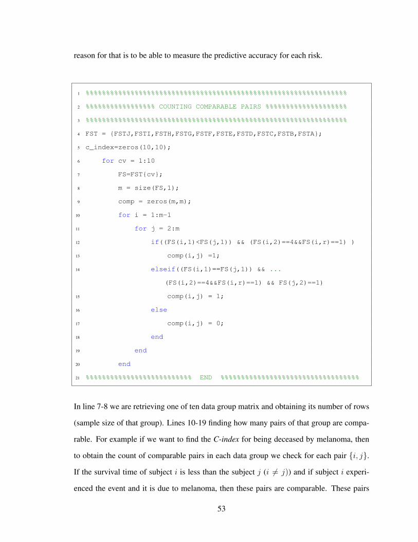
reason for that is to be able to measure the predictive accuracy for each risk.

1 %%%%%%%%%%%%%%%%%%%%%%%%%%%%%%%%%%%%%%%%%%%%%%%%%%%%%%%%%%%%%%%%

2 %%%%%%%%%%%%%%%%% COUNTING COMPARABLE PAIRS %%%%%%%%%%%%%%%%%%%%

3 %%%%%%%%%%%%%%%%%%%%%%%%%%%%%%%%%%%%%%%%%%%%%%%%%%%%%%%%%%%%%%%%

4 FST = {FSTJ,FSTI,FSTH,FSTG,FSTF,FSTE,FSTD,FSTC,FSTB,FSTA};

5 c_index=zeros(10,10);

6 for cv = 1:10

7 FS=FST{cv};

8 m = size(FS,1);

9 comp = zeros(m,m);

10 for i = 1:m-1

11 for j = 2:m

12 if((FS(i,1)<FS(j,1)) && (FS(i,2)==4&&FS(i,r)==1) )

13 comp(i,j) =1;

14 elseif((FS(i,1)==FS(j,1)) && ...

(FS(i,2)==4&&FS(i,r)==1) && FS(j,2)==1)

15 comp(i,j) = 1;

16 else

17 comp(i,j) = 0;

18 end

19 end

20 end

21 %%%%%%%%%%%%%%%%%%%%%%%%%% END %%%%%%%%%%%%%%%%%%%%%%%%%%%%%%%%%%

In line 7-8 we are retrieving one of ten data group matrix and obtaining its number of rows

(sample size of that group). Lines 10-19 finding how many pairs of that group are compa-

rable. For example if we want to find the C-index for being deceased by melanoma, then

to obtain the count of comparable pairs in each data group we check for each pair {i, j}.

If the survival time of subject i is less than the subject j (i 6= j)) and if subject i experi-

enced the event and it is due to melanoma, then these pairs are comparable. These pairs

53

are also comparable if their survival times are equal and subject i experienced the event

due to melanoma plus subject j also experienced the event. Otherwise the two pairs are

not comparable. Now we move to determining the concordant pairs based on the network

outcome for each time period.

1 conc = zeros(m,m);

2 yy=prediction{hn,cv};

3 for i = 1:m-1

4 for j = 2:m

5 if((FS(i,1)<FS(j,1)) && (FS(i,2)==4&&FS(i,4)==1))

6 if(yy(i,pre)>yy(j,pre))

7 conc(i,j)=1*comp(i,j);

8 else

9 conc(i,j)=0;

10 end

11 end

12 end

13 end

14 sconc = sum(sum(conc));

15 scomp = sum(sum(comp));

16 c = sconc/scomp;

17 end

The code for counting the number of concordant pairs is shown on the next page. The

number of concordant pairs is determined if for each comparable pair {i, j} the predicted

hazard of i is larger than the predicted hazard of j, such that subject i experienced the event

while subject j did not, lines 5-19 of code on next page. On the second line we obtain

the prediction done with each neural network structure for each of the ten data groups.

The whole counting process of comparable pairs and concordant pairs are repeated for the

different number of neural networks trained with different number of hidden units. The

54

same process was applied to all neural networks trained with each of the three learning

techniques.

4.5.2 Comparison with C-index

Table 9: C-index for first time interval for female patients

Risk 1:Deceased by MelanomaTI LA HN Data groups

1 2 2 3 5 6 7 8 9 10

1

Evid

4 0.9509 0.9478 0.9458 0.9480 0.9391 0.9487 0.9432 0.9465 0.9439 0.94955 0.9477 0.9424 0.9505 0.9460 0.9419 0.9498 0.9366 0.9534 0.9460 0.94676 0.9490 0.9435 0.9456 0.9453 0.9434 0.9498 0.9416 0.9504 0.9424 0.95147 0.9415 0.9412 0.9417 0.9403 0.9342 0.9483 0.9384 0.9448 0.9451 0.95268 0.9395 0.9421 0.9468 0.9457 0.9433 0.9497 0.9375 0.9505 0.9405 0.94939 0.9436 0.9434 0.7965 0.9422 0.9344 0.9467 0.9411 0.9523 0.9440 0.945410 0.9457 0.9424 0.9469 0.9455 0.9414 0.9484 0.9417 0.9476 0.9424 0.944711 0.9401 0.9403 0.9430 0.9438 0.9353 0.9461 0.9397 0.9503 0.9389 0.951212 0.9497 0.9382 0.9416 0.9442 0.9387 0.9428 0.9327 0.9518 0.9401 0.948513 0.9461 0.9430 0.9382 0.9443 0.9394 0.9518 0.9312 0.9469 0.9417 0.9481

HMC

4 0.9419 0.9410 0.9438 0.9442 0.9385 0.9459 0.9393 0.9489 0.9414 0.94905 0.9487 0.9405 0.9429 0.9449 0.9391 0.9494 0.9397 0.9492 0.9407 0.94896 0.9432 0.9385 0.9416 0.9422 0.9377 0.9452 0.9358 0.9460 0.9414 0.94847 0.9420 0.9399 0.9472 0.9468 0.9387 0.9440 0.9376 0.9514 0.9426 0.94878 0.9412 0.9405 0.9435 0.9462 0.9389 0.9495 0.9383 0.9485 0.9392 0.94969 0.9440 0.9395 0.9444 0.9449 0.9367 0.9467 0.9376 0.9486 0.9397 0.9493

10 0.9425 0.9399 0.9452 0.9438 0.9378 0.9443 0.9387 0.9460 0.9416 0.946211 0.9424 0.9382 0.9431 0.9421 0.9373 0.9453 0.9360 0.9447 0.9395 0.949212 0.9422 0.9389 0.9429 0.9441 0.9389 0.9467 0.9384 0.9454 0.9393 0.948213 0.9407 0.9405 0.9419 0.9429 0.9366 0.9448 0.9367 0.9471 0.9387 0.9490

EHMC

4 0.9447 0.9407 0.9436 0.9448 0.9389 0.9460 0.9397 0.9501 0.9430 0.94955 0.9444 0.9420 0.9453 0.9460 0.9399 0.9473 0.9406 0.9509 0.9427 0.94946 0.9419 0.9423 0.9443 0.9444 0.9416 0.4025 0.9399 0.9481 0.9412 0.95027 0.9423 0.9393 0.9441 0.9429 0.9385 0.9462 0.9380 0.9483 0.9401 0.94858 0.9429 0.9386 0.9432 0.9434 0.9364 0.9462 0.9373 0.9461 0.9397 0.94739 0.9440 0.9395 0.9444 0.9449 0.9367 0.9467 0.9376 0.9486 0.9397 0.9493

10 0.9425 0.9399 0.9452 0.9438 0.9378 0.9443 0.9387 0.9460 0.9416 0.946211 0.9424 0.9382 0.9431 0.9421 0.9373 0.9453 0.9360 0.9447 0.9395 0.949212 0.9422 0.9389 0.9429 0.9441 0.9389 0.9467 0.9384 0.9454 0.9393 0.948213 0.9407 0.9405 0.9419 0.9429 0.9366 0.9448 0.9367 0.9471 0.9387 0.9490

We want to test how good our new neural network performs as to predicting the sur-

vival time of competing risks. Additionally, we want to find the best learning algorithm

that yields better learning for neural network. We use the C-index to validate our new ap-

proach (DHANN-CR) and the new learning algorithms. For each of the ten data groups

of males and females, we tried eleven neural network structures starting with four hidden

55

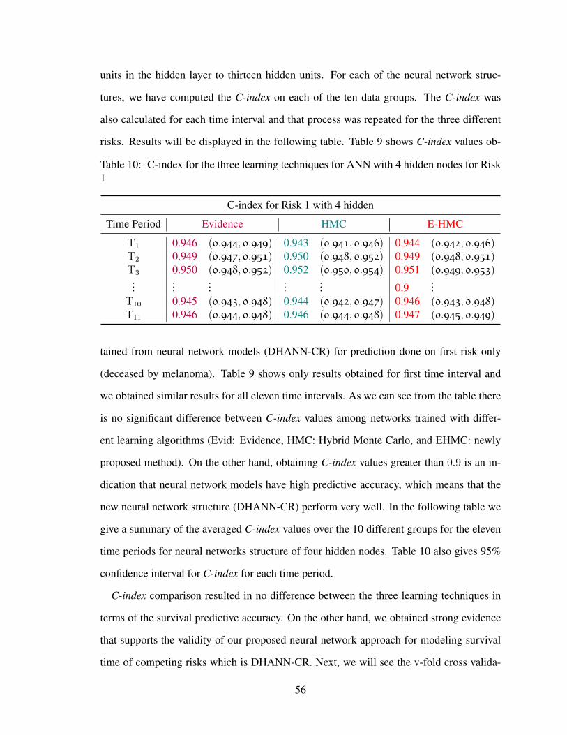
units in the hidden layer to thirteen hidden units. For each of the neural network struc-

tures, we have computed the C-index on each of the ten data groups. The C-index was

also calculated for each time interval and that process was repeated for the three different

risks. Results will be displayed in the following table. Table 9 shows C-index values ob-

Table 10: C-index for the three learning techniques for ANN with 4 hidden nodes for Risk1

C-index for Risk 1 with 4 hidden

Time Period Evidence HMC E-HMC

T1 0.946 (0.944, 0.949) 0.943 (0.941, 0.946) 0.944 (0.942, 0.946)T2 0.949 (0.947, 0.951) 0.950 (0.948, 0.952) 0.949 (0.948, 0.951)T3 0.950 (0.948, 0.952) 0.952 (0.950, 0.954) 0.951 (0.949, 0.953)...

......

...... 0.9

...T10 0.945 (0.943, 0.948) 0.944 (0.942, 0.947) 0.946 (0.943, 0.948)T11 0.946 (0.944, 0.948) 0.946 (0.944, 0.948) 0.947 (0.945, 0.949)

tained from neural network models (DHANN-CR) for prediction done on first risk only

(deceased by melanoma). Table 9 shows only results obtained for first time interval and

we obtained similar results for all eleven time intervals. As we can see from the table there

is no significant difference between C-index values among networks trained with differ-

ent learning algorithms (Evid: Evidence, HMC: Hybrid Monte Carlo, and EHMC: newly

proposed method). On the other hand, obtaining C-index values greater than 0.9 is an in-

dication that neural network models have high predictive accuracy, which means that the

new neural network structure (DHANN-CR) perform very well. In the following table we

give a summary of the averaged C-index values over the 10 different groups for the eleven

time periods for neural networks structure of four hidden nodes. Table 10 also gives 95%

confidence interval for C-index for each time period.

C-index comparison resulted in no difference between the three learning techniques in

terms of the survival predictive accuracy. On the other hand, we obtained strong evidence

that supports the validity of our proposed neural network approach for modeling survival

time of competing risks which is DHANN-CR. Next, we will see the v-fold cross valida-

56

tion comparison that will compare between the three learning techniques by looking at the

errors.

4.5.3 Comparison with v-fold Cross Validation

In this section, we compare the errors obtained by DHANN-CR trained with three different

learning algorithms. We would like to recall that all networks started with the same initial

values of hyperparamters which is 0.01. Also we used the ARD, which means that each of

our eleven inputs is assumed to be controlled by weights having different distributions.

1 2 3 4 5 6 7 8 9 10 119.5

9.6

9.7

9.8

9.9

10

10.1

10.2

10.3

10.4

x 105

Data Group

Cost F

unctio

n

Over all error for different ANN models, trained with HMC

4 hn5 hn6 hn7 hn8 hn9 hn10 hn11 hn12 hn13 hn

Figure 14.: Errors distribution for neural networks trained with 11 different values ofhidden nodes with ten different data, using Hybrid Monte Carlo Sampling

We start with neural networks trained with Hybrid Monte Carlo Sampling as it resulted

in the highest error (between 9.6 ∗ 105 to 10.4 ∗ 105). Figure 14 shows the amount of error

(Y − axis) obtained from neural network trained on different groups (X − axis) of data

using the same learning algorithm.

57

1 2 3 4 5 6 7 8 9 10 11

3.5

3.6

3.7

3.8

3.9

4

4.1

4.2

4.3

4.4x 10

4 Cost Function for ANN models trained with Evidence

Data Group

Cost

Function

4 hn5 hn6 hn7 hn8 hn9 hn10 hn11 hn12 hn

Figure 15.: Errors distribution for neural networks trained with 11 different values ofhidden nodes with ten different data, using Evidence Procedure

1 2 3 4 5 6 7 8 9 10 116000

6500

7000

7500

8000

8500

9000

9500

10000Cost Function for ANN models trained with E−HMC

Data Groups

Co

st

Fu

nctio

n

4 hn5 hn6 hn7 hn8 hn9 hn10 hn11 hn12 hn13 hn

Figure 16.: Errors distribution for neural networks trained with 11 different values ofhidden nodes with ten different data, using E-Hybrid Monte Carlo

We wish to mention that this amount of error is for predicting the hazard probability

function for 6644 patients, that is, the total number of predictions is 6644*11=73084 for

58

the female data. The average error using the Hybrid Monte Carlo Sampling is between

13.092 and 14.282, which is not what we expect for an average error to be. In addition,

the errors for the same neural network structures are not constant, having variations, rather

than having constant behavior on different data sets.

This explains what we mentioned before using HMC requires the knowledge of the cor-

rect prior values. One could get better models using HMC by trying different initial values

for hyperparameters, but the cost of computational time it takes to run HMC for one model

makes it unrealistic to continue. We must mention that Neal [45] had generated 2 million

networks to fit a function with 6 data points. In Figure 15, we present the errors distribu-

tion using evidence procedure on the same data set as HMC. Note that the errors decreased

compared to networks trained with HMC, their variance is with less variability compared

to HMC. Figure 16 shows the errors of neural networks prediction, that was trained with

our newly proposed method, which is Using the evidence to re-estimate hyperparameters

based on the data and then use Hybrid Monte Carlo sampling to obtain samples of the

weights distribution from its posterior. As we can see, errors are fewer compared to neural

networks trained with Evidence and HMC. Also, errors seems more consistent for different

data groups. As the number of hidden nodes increases, error also increase, giving an advan-

tage for using Bayesian learning with neural network no need for large number of hidden

units. By looking at the errors of neural networks with five hidden units in the hidden layer

(of figure 15) possesses errors with lower variance, have approximately constant variance

compared to others. The best fit neural network model for predicting survival time of com-

peting risks is the model trained with E-HMC with five hidden units in hidden layer. All

results shown above are for female melanoma patient data, similar results were obtained

for male patient data.

59

4.6 Conclusion

In the current Chapter, we have obtained several important results using artificial neural

network for predicting survival time of competing risks. We summarize our findings in the

following points:

1. We have presented a new method that utilize artificial neural network in predicting the

hazard function of competing risks.

2. We are introducing (proposing) a solution to help use the Hybrid Monte Carlo simula-

tion learning algorithm for neural network in a more efficient way.

3. Using Bayesian inference in the learning of neural networks avoids the need of large

number of hidden units in hidden layer.

The DHANN-CR is a new method of utilizing ANN in survival analysis. It’s more useful

compared to PLANN,and PLANN-CR especially with the existence of huge data set. The

use of Bayesian inference in learning neural network, gives neural network more chance to

learn than to memorize, increasing the number of hidden units in neural networks makes

it more memorizing tool rather than learning tool. Our future goal is to see if our new

proposed learning method can be utilized with artificial neural network in other statistical

analysis methods, such as time series analysis, and Categorical data analysis, among others.

In the next Chapter, we introduce a new approach of using Hybrid Monte Carlo Sampling

with recurrent neural network for the modeling of time series data.

60

Chapter 5

Artificial Neural Network for Forecasting Carbon Dioxide Emission in the

Atmosphere

In this Chapter, we develop an artificial neural network model utilizing time series approach

for forecasting Carbon dioxide, CO2, in the atmosphere . In Chapter three and four we saw

the use of Feedforward artificial neural network in survival analysis, however, Feedforward

networks can be used in other generalized linear statistical modeling [65–68]. One of the

important statistical analysis methods is time series analysis, which deals with forecasting

observation in the future for a certain time period that mainly depends on the same reading

of that observation on previous time periods. That is, the future predictions depends on

previous observations of the same data. Modeling of such situations in ANN requires

the use of recurrent neural networks. In this Chapter we will present a new method of

using Hybrid Monte Carlo Sampling in the learning of recurrent networks for time series

forecasting. We will validate the new proposed model on a popular and vital problem our

society is facing, which is carbon dioxide emission in the atmosphere.

Carbon dioxide is strongly connected to climate change, but the impact of carbon diox-

ide varies according to the source and level of emissions and also according to regional

effects,[69]. As we know, the most dominant source for carbon dioxide emission is fossil

fuels, making it a major contributing factor in global warming. Other variables that con-

tribute towards the emission of carbon dioxide in the atmosphere are given in Figure 16,

[70]. Our future goal is to use artificial neural network to build a model that better under-

stand the contribution of each of the variables in Figure 17 , and hence be able to make

policies and control the emission of carbon dioxide. United States comes in second place

61

after China in the ten largest carbon dioxide emitters. United States shares about 14.69%

of Global carbon dioxide emission compared to China of 23.43% in year 2014, [71]. Our

work starts by fitting a neural network model for predicting the monthly average carbon

dioxide emission in United States.

Figure 17.: Emission of Carbon Dioxide in the Atmosphere in U.S.A.

5.1 Literature Review

There is a number of studies utilizing artificial neural network for the prediction of time

series data, making it too hard to track. Models ranging from the use of Feedforward net-

works to recurrent networks and lately using what is called by wavelet neural network,

[72]. One of the most popular series used for forecasting time series is the sunspot series,

62

a recent study on using neural network with quantum gate was proposed by X. Guan et. al,

[73]. The authors of the study presented an improvement for predicting sunspot number

series, however no further investigation for testing their model on other time series data.

This has been the issue of utilizing neural networks in time series for the last decade. The

use of neural networks in time series depends heavily on the data, different models, differ-

ent architecture of networks were presented some showed better performance compared to

the popular ARIMA model others did not, [74]. Fitting ANN model for time series data

involves not only finding optimal numbers of hidden units, as it was the case in Chapters 3

& 4, but also the number of input units is variant. The number of input units in forecast-

ing models corresponds to number of previous observations that one would use to predict

future outcome. There is no specific method of choosing the number of input units, while

researchers tried to find a solution to this problem, one was a claim of choosing the number

of hidden units is equal to number of auto-regressive(AR) terms in Box-Jenkins [75]. How-

ever, this approach can not be useful as for moving average of order one, MA(1), model

there is no autoregressive terms. Another solution was to use Box and Jenkins model iden-

tification procedure and then use the number of input terms corresponding to the identified

terms. For example, if Box and Jenkins model identification step found AR(2) and MA(1),

then the ANN used for such a model would probably have three input nodes, for Xt−2 and

et−1. In a study by Zou et al. [76], compared between performance of ARIMA, ANN and

a combined ARIMA, ANN model. In which they used ARIMA to identify AR and MA

terms, then use ANN with number of input units equal to number of identified terms from

ARIMA model. According to their comparison it was found that the combined ANN and

ARIMA model resulted in less mean square error, however, results may vary with different

data set. In general there is no specific procedure for the choice of a certain neural net-

work structure for time series analysis, it all depends on the data series. The second part

of utilizing ANN in time series involves the choice of learning algorithm. Several learn-

ing algorithms were used and proposed in literature, like the use of genetic algorithms as

63

in, [77–80], while others used regular back-propagation algorithms that were summarized

along with results in [74]. On the other hand some other models used the evidence proce-

dure that was proposed by Mackay [43]. J. Ticknor used evidence procedure along with

a three layer Feedforward network to forecast the stock market, [81]. However, Ticknor

did not use the evidence, as explained in Chapter 2, to compare between neural network

models to chose the optimal number of hidden units.

The aim of the present study is to reduce the issues that needs attention for utilizing ANN

in time series. We propose the use of recurrent neural network that utilizes Hybrid Monte

Carlo sampling learning algorithm by applying it online. In other words, for each input we

update the learning of neural networks. The purpose of using HMC is to fix the number of

hidden units,as we discussed in Chapter 4 that the networks trained with HMC, does not

require large number of hidden units. In the coming sections we highlight the important

points of the ARIMA model, then we explain the proposed neural network structure and

the developing of a new learning algorithm written for this specific task. The learning

algorithm involves the use of HMC algorithm written by Nabney in the NETLAB package

for MATLAB software.

5.1.1 Auto-Regressive Integrated Moving Average Models: ARIMA

The auto-regressive integrated moving average (ARIMA) models are the most popular time

series methods for modeling stationary time series. ARIMA initially was presented by Box

and Jenkins in 1970 [82]. Let {Xt, Xt−1, Xt−2, ..., X1} be a time series data, the general

mathematical expression of the ARIMA model is given by:

Φp(B)(1−B)dXt = a+ Θq(B)εt (5.1)

where Φp(B) is the autoregressive operator with order p defined as

64

Φp(B) = 1− φ1B − φ2B2 − · · · − φpBp

where Θq(B) is the moving average operator with order q defined as

Θp(B) = 1− θ1B − θ2B2 − · · · − θqB q

where B is the back shift operator, εt is the error term that is normally distributed with

mean zero and constant variance. If the time series data shows a seasonal trend, then a

generalization of the ARIMA model is to fit seasonal data is called Seasonal autoregressive

integrated moving average model (SARIMA) given by:

Φp(B)ΦP (Bs)(1−B)D(1−B)dXt = a+ Θq(B)ΘQ(Bs)εt (5.2)

where ΦP (Bs) and ΘQ(Bs) are the seasonal autoregressive and moving average, respec-

tively. The procedure that we follow to fit the ARIMA or SARIMA models know as the

Box and Jenkins procedure can be summarized into the following steps.

1. Model Identification: In which the order of AR(p) and MA(q) are identified. By com-

puting and plotting the autocorrelation function (ACF) and the partial autocorrelation

function (PACF). If the series is non-stationary then it may requires filtering (either by

non-seasonal or seasonal difference), and if series possesses a non constant variance

over time then a transformation may take place.

2. Model Estimation: After step 1 is done, and the series is made sure to be station-

ary (As required by ARIMA procedure), then it follows estimation of the parameters

φ1, φ2, ..., φp and/or θ1, θ2, ..., θq using maximum likelihood estimation to minimize the

mean square error function.

3. Model Validation: Includes tests for white noise errors (making sure errors follows

the assumed distribution) by checking errors autocorrelation and partial autocorrelation

functions. Additionally, the use of Akaike information criterion, [83](AIC), to compare

among several models.

65

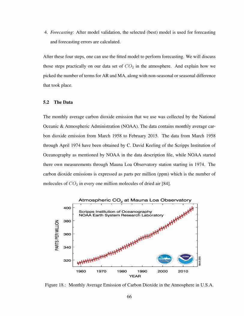
4. Forecasting: After model validation, the selected (best) model is used for forecasting

and forecasting errors are calculated.

After these four steps, one can use the fitted model to perform forecasting. We will discuss

those steps practically on our data set of CO2 in the atmosphere. And explain how we

picked the number of terms for AR and MA, along with non-seasonal or seasonal difference

that took place.

5.2 The Data

The monthly average carbon dioxide emission that we use was collected by the National

Oceanic & Atmospheric Administration (NOAA). The data contains monthly average car-

bon dioxide emission from March 1958 to February 2015. The data from March 1958

through April 1974 have been obtained by C. David Keeling of the Scripps Institution of

Oceanography as mentioned by NOAA in the data description file, while NOAA started

there own measurements through Mauna Loa Observatory station starting in 1974. The

carbon dioxide emissions is expressed as parts per million (ppm) which is the number of

molecules of CO2 in every one million molecules of dried air [84].

Figure 18.: Monthly Average Emission of Carbon Dioxide in the Atmosphere in U.S.A.

66

Figure 18 , displays the monthly average emissions of CO2 in the atmosphere in the

U.S.A, obtained from NOAA website [84]. In the current analysis we use information

from January 1960 to December 2008 to train the ANN model, and left the remaining to

test the forecasting accuracy of our models. Data entering neural network is required to be

on small scale to smooth and faster conversion. We did standarized carbon dioxide data

using the following formula:

xnewi =xi −min{xt, xt−1, · · · , x1}

max{xt, xt−1, · · · , x1} −min{xt, xt−1, · · · , x1}(5.3)

5.3 Time Series Data Modeling

In this study we present a model by combining both the ARIMA and ANN. We are going to

use the first step in the ARIMA procedure to identify the number of input units in the input

layer. Then, we will train a recurrent neural network using Hybrid Monte Carlo Sampling

using online learning. First we start with model identification.

5.3.1 Model Identification

Based on Box and Jenkins methodology, a time series data should be stationary, so the first

step in model identification is to make sure that the series is stationary, and this is done by

looking at the time series plot of the data.

By looking at Figure 19, we notice that as time increases the series also increase suggest-

ing a possible first nonseasonal difference(filtering) is needed as the average of the series is

not constant over fixed time periods. So we take the first difference and then plot the series

again. As we can see in Figure 20, the series now shows constant mean making it station-

ary with respect to mean. It also appear that there exist a seasonal trend, in which its order

will be determined by looking at the autocorrelation function and partial autocorrelation

function.

67

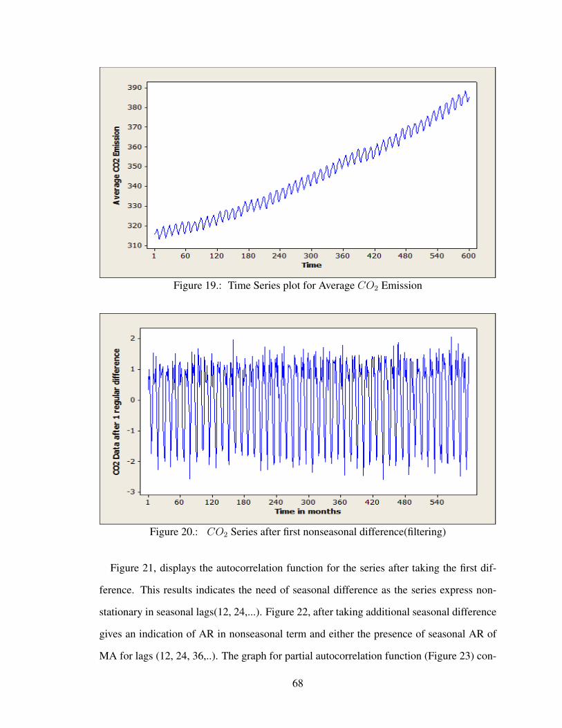
Figure 19.: Time Series plot for Average CO2 Emission

Figure 20.: CO2 Series after first nonseasonal difference(filtering)

Figure 21, displays the autocorrelation function for the series after taking the first dif-

ference. This results indicates the need of seasonal difference as the series express non-

stationary in seasonal lags(12, 24,...). Figure 22, after taking additional seasonal difference

gives an indication of AR in nonseasonal term and either the presence of seasonal AR of

MA for lags (12, 24, 36,..). The graph for partial autocorrelation function (Figure 23) con-

68

Figure 21.: Autocorrelation function of CO2 Series after first difference

firms that we have AR of order one in the non-seasonal part and a MA of order one in sea-

sonal part. Figure 22, plots the autcorrelation function for series after taking 1 non-seasonal

difference and one seasonal difference. Figure 23 plots the partial autocorrelation function

for the same series. The ACF behavior for AR model and MA model is the same, while

the difference will be obtained from the partial autocorrelation function. Since, in partial

autocorrelation function we have one term above zero, then it is an indication of AR(1)

model. The seasonal lags in Figure 22 and Figure 23 gives the indication of a seasonal

term in SMA(1). Overall, model identification suggests the best model of the following

form

SARIMA(1,1,0)x(0,1,1)12, that is,

Φ1(B)(1−B)1(1−B)1Xt = a+ ΘQ(B)εt (5.4)

with 1 nonseasonal difference and one seasonal difference, and with one nonseasonal

AR(1) with one seasonal MA (SMA(1)).

So for fitting the neural network model to CO2 data, we are going to use three input

units in the input layer. Since we have identified one nonseasonal difference we will take

69

Figure 22.: Autocorrelation function after taking one seasonal difference

Table 11: SARIMA model Estimates using Minitab

Parameter Estimate SE T-value P-ValueAR(1) -0.2858 0.0398 -7.17 0.000

SMA(12) 0.9190 0.0166 55.32 0.000

constant 0.00283 0.00119 2.37 0.018

MSE 0.0864

into consideration two previous valuesXt−1andXt−2 to predictXt along with one seasonal

moving average εt−12. The moving average term will be represented by the recursive prop-

erty of neural network. We have fitted the model in (5.3) using Minitab Statistical Software

and obtained the results in Table 11.

5.3.2 Recurrent Neural Network for CO2 Data

To fit the CO2 data we decided to choose three input units in the input layer, two for two

successive data points in the past to predict the next outcome. The third one is fed from the

error observed by the neural network outcome as it is shown in Figure 24. We will discuss

how the data is restructured to be trained correctly using the recurrent neural network in

70

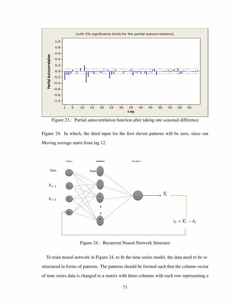
Figure 23.: Partial autocorrelation function after taking one seasonal difference

Figure 24. In which, the third input for the first eleven patterns will be zero, since our

Moving average starts from lag 12.

Figure 24.: Recurrent Neural Network Structure

To train neural network in Figure 24, to fit the time series model, the data need to be re-

structured in forms of patterns. The patterns should be formed such that the column vector

of time series data is changed to a matrix with three columns with each row representing a

71

pattern.

1 %%%%%%%%%%%%%%%%%%%%%%%%%%%%%%%%%%%%%%%%%%%%%%%%%%%%%%%%%%%%%%%%%

2 %%% Restructuring of Time Series data for Neural Network%%%%%%%%

3 %%%%%%%%%%%%%%%%%%%%%%%%%%%%%%%%%%%%%%%%%%%%%%%%%%%%%%%%%%%%%%%%%

4 function [Xtrain, YTrain] = restructure(nin,nout,data,nloop,lag)

5 k1 =1;

6 n = size(data);

7 r=lag-1

8 t=nin-nloop

9 Xtrain=zeros(1,nin);

10 YTrain=zeros(nout,1);

11 while (k1≤n)

12 target(nout,1)=data(k1+t,1);

13 for i = 1:(t)

14 tem(1,i)=data(k1+i-r,1);

15 end

16 if(nloop = 1)

17 tem(1,nin)=0; % If you will be looping an error or predicted ...

value

18 end;

19 Xtrain=vertcat(Xtrain,tem);

20 YTrain=vertcat(YTrain,target);

21 k1=k1+1;

22 i=1;

23 end

For example, the first row will consist of

X1, X2, and (ε−9 = 0) to predict X3,

next row will consist of

X2, X3, and (ε−8 = 0) to predict X4,

72

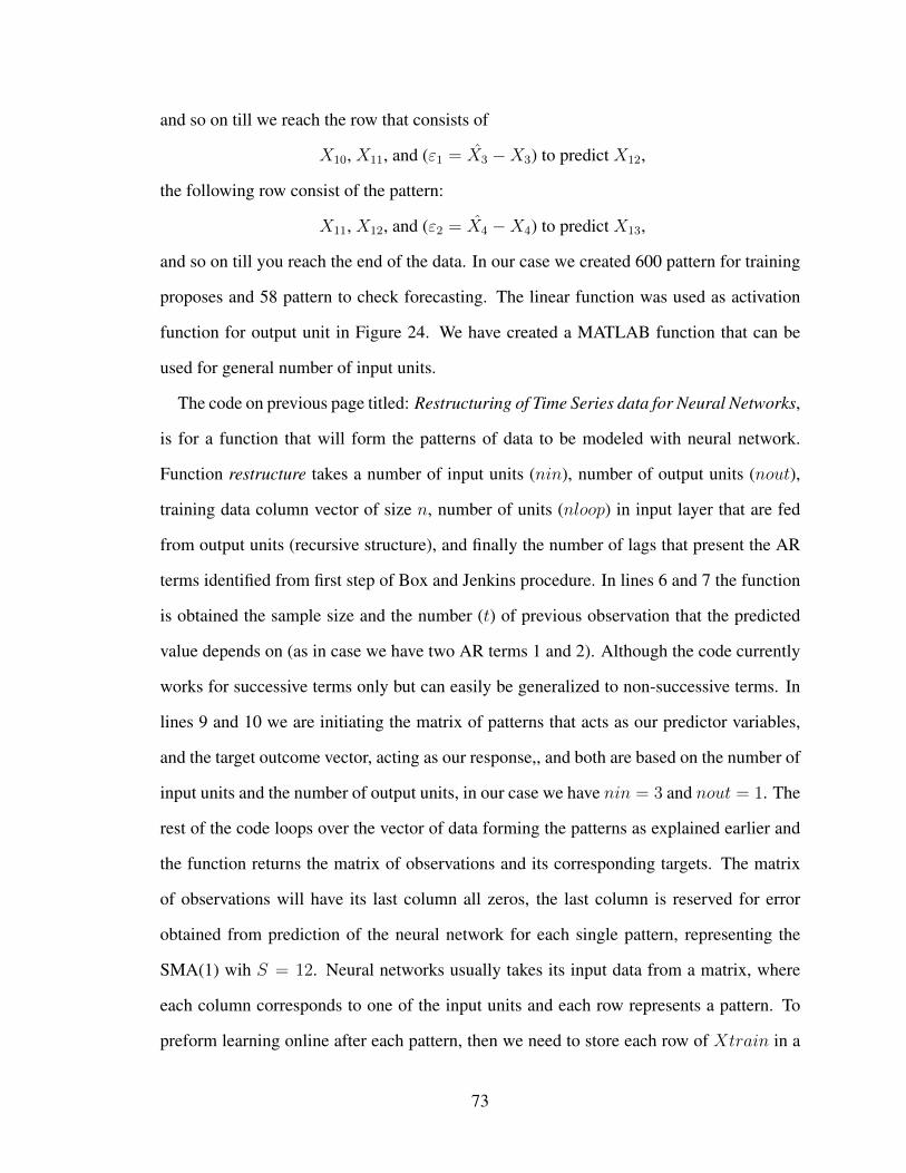
and so on till we reach the row that consists of

X10, X11, and (ε1 = X3 −X3) to predict X12,

the following row consist of the pattern:

X11, X12, and (ε2 = X4 −X4) to predict X13,

and so on till you reach the end of the data. In our case we created 600 pattern for training

proposes and 58 pattern to check forecasting. The linear function was used as activation

function for output unit in Figure 24. We have created a MATLAB function that can be

used for general number of input units.

The code on previous page titled: Restructuring of Time Series data for Neural Networks,

is for a function that will form the patterns of data to be modeled with neural network.

Function restructure takes a number of input units (nin), number of output units (nout),

training data column vector of size n, number of units (nloop) in input layer that are fed

from output units (recursive structure), and finally the number of lags that present the AR

terms identified from first step of Box and Jenkins procedure. In lines 6 and 7 the function

is obtained the sample size and the number (t) of previous observation that the predicted

value depends on (as in case we have two AR terms 1 and 2). Although the code currently

works for successive terms only but can easily be generalized to non-successive terms. In

lines 9 and 10 we are initiating the matrix of patterns that acts as our predictor variables,

and the target outcome vector, acting as our response,, and both are based on the number of

input units and the number of output units, in our case we have nin = 3 and nout = 1. The

rest of the code loops over the vector of data forming the patterns as explained earlier and

the function returns the matrix of observations and its corresponding targets. The matrix

of observations will have its last column all zeros, the last column is reserved for error

obtained from prediction of the neural network for each single pattern, representing the

SMA(1) wih S = 12. Neural networks usually takes its input data from a matrix, where

each column corresponds to one of the input units and each row represents a pattern. To

preform learning online after each pattern, then we need to store each row of Xtrain in a

73

separate row vector and this is done by storing Xtrain in a cell array as it is shown in the

following code, same is also made for the target vector.

1 for i = 1:n

2 Xi{i,1}=Xtrain(i,1:nin);

3 Ti{i,1}=YTrain(i,1);

4 end

Once we have the cell array ready, next initialize the network and start training it using

Hybrid Monte Carlo Sampling as follows:

1 %initialize neural network

2 nin= 3;

3 nout=1;

4 nhidden=10;

5 %Assigning values for hyperparameters

6 aw1 = [0.01, 0.01, 0.5]; %3 different distributions for input units

7 ab1 = 0.01; %hyperparameter for bias of first layer

8 aw2 = 0.01; %hyperparameter for weights fanning from hidden to ...

output layer

9 ab2 = 0.01; %hyperparameter for bias of hidden layer

10 beta = 50; % hyperparameter for data error

11 prior = mlpprior(nin, nhidden, nout, aw1, ab1, aw2, ab2);

12 net = mlp(nin, nhidden, nout, 'linear',prior,beta);

13 % Start loop to preform Online training

14 for j =1:600

15 seed = 10; % Seed for random weight ...

initialization.

16 rng(seed,'v5uniform');

17 rng(seed,'v5normal');

18 % Set up vector of options for hybrid Monte Carlo.

74

19 nsamples = 500; % Number of retained samples.

20 options = foptions; % Default options vector.

21 options(1) = 1; % Switch on diagnostics.

22 options(5) = 1; % Use persistence

23 options(7) = 25; % Number of steps in trajectory.

24 options(14) = nsamples; % Number of Monte Carlo samples returned.

25 options(15) = 200; % Number of samples omitted at start of chain.

26 options(17) = 0.75; % Alpha value in persistence

27 options(18) = 0.002; % Step size.

28 w = mlppak(net);

29 % Initialise HMC

30 hmc('state', 42);

31 %Calling HMC after feeding network with each pattern (Online ...

learning)

32 [samples, energies] = hmc('neterr', w, options, 'netgrad', net, ...

Xi{j}, Ti{j});

33 pred = zeros(size(Ti{j}));

34 Ed = 0;

35

36 for k = 1:nsamples

37 w2 = samples(k,:);

38 net2 = mlpunpak(net, w2);

39 network11{1,k}=net2;

40 Y = mlpfwd(net2, Xi{j});

41 [Err, edata, eprior] = mlperr(net2, Xi{j},Ti{j});

42 % Average sample predictions as Monte Carlo estimate of true ...

integral

43 pred = pred + Y;

44 Ed = Ed + edata;

45 end

46 pred = pred./nsamples;

47 Ed=Ed./nsamples;

75

48 err(j)=Ed;

49 %Updating the patterns with error obtained from previous predictions

50 Xi{j+11,1}(1,3)=Ed;

51 end

Lines 2-12: the network is being structured and the prior object is built up. We used the

automatic relevance determination to assign different distribution of weights for each of

our three input units, line 6, error hyperparameter value is 0.5. Line 12: the neural network

is set with the choice of input units, output units, linear function as activation function for

output unit and prior structure. Then online learning is applied by calling the Hybrid Monte

Carlo sampling for each record of the cell array Xi with corresponding targets Ti. Errors

are computed after each pattern and input cell array is updated, lines 46-50. In the current

analysis the error obtained from the first pattern of Xi is returned and stored in the 12th

pattern of Xi completing the third input information, corresponding to SMA(1). Lines 15-

44 are taken from Nabney algorithm for HMC implementation, more details can be found

in his book [62]. We sampled 500 samples for each pattern using HMC.

5.4 Results

As we mentioned in Chapter 2 the use of Hybrid Monte Carlo Sampling requires several

trails to obtain initial values for hyperparameters. We will present two graphs to illus-

trate the difference between the initial values of hyperparameters. After training the neu-

ral network with the previously mentioned procedure we obtained a mean square error of

0.000616, by comparing it with the one obtained from using SARIMA model in Table 9

(MSE = 0.0864) we can tell that the recurrent neural network model outperformed the

SARIMA model. After we compared SARIMA and the recurrent neural network trained

with HMC, we also compare their forecasting accuracy. As we mentioned in the data sec-

tion that we left five years for determining the forecasting accuracy.

76

Figure 25.: Comparison between forecasting accuracy of RANN with (0.01 hyperparame-ters) and SARIMA

Figure 26.: Comparison between forecasting accuracy of RANN and SARIMA

77

In Figure 25, Black dots are for observed CO2 average monthly emission, while red dots

from the SARIMA model. The green series is the forecasting from (RANN) trained with

initial values of hyperparameters of the input units all equal to 0.01. We have realized that

the third input unit that corresponds to the error needs to have higher value of hyperparam-

eter, meaning errors have less weight compared to X1 and X2 in forecasting X3. The final

neural network we developed is the one trained with initial values of hyperparameters of

0.01 for two data inputs and 0.5 for the error input.

Figure 26, displays the final outcome of the best fit neural network. The red series here

represents the forecasting of the RANN, it is either similar to SARIMA model in some

cases and in others it outperform it.

5.5 Conclusion

Our main objective in this Chapter is to introduce a general framework for utilizing neural

network in time series analysis. Step 1 in achieving our objective, we proposed a new

methodology for utilizing ANN in fitting stationary time series data. The proposed method

resulted in better performance compared to the popular ARIMA model. Step 2 is to model

non-stationary time series data using same method (Taking into account the high capability

of neural network in fitting non-linear patterns). We would like to mention that we first

tried using the evidence HMC method (The new proposed Bayesian learning presented in

chapter 4) in training the recurrent neural network in Figure 24, but we could not observe

any accepted samples from the HMC after re-estimating the hyperparameters using the

evidence. Thus, the evidence procedure do not perform well with online learning.

The secondary objective of the current study, is to better understand the behavior of CO2

in the atmosphere. Additionally form a model that predicts carbon dioxide emission from

the various source in Figure 17. Also, use the automatic relevance determination to rank

these sources based on their percentage of contribution to carbon dioxide emission.

78

5.5.1 Contributions

The development of ANN models for time series analysis revealed some very important

findings that can be summarized as follows:

1. The use of ARMIA model identification step is important in determining the number

of input units in neural networks used to model time series data.

2. Best neural network structure to model time series data is recurrent (recursive) neural

networks.

3. The Hybrid Monte Carlo Sampling proposed by Neal, train perfectly recurrent neural

networks.

4. Carbon dioxide emission in the atmosphere can be better explained through a recurrent

neural network model trained with Hybrid Monte Carlo Sampling compared to popular

ARIMA model.

79

Chapter 6

Future Work

Our future work consist of two main goals, first is to introduce Bayesian techniques to

other artificial intelligence methods such as genetic algorithm, among others. The second

is to use artificial neural network with Bayesian techniques to find a solution for other vital

problems our society is facing.

6.1 Neural Network models in Cancer research

Our proposed model can be used with other cancer diseases, such as lung cancer, breast

cancer, brain cancer, among others. For example, in survival studies, treatment options can

be added to risk factors, and by the use of automatic relevance determination, doctors can

suggest patients their suitable course of treatment that would make them survive longer. Of

course these kind of models need to be trained on more specialized data than the one with

used in chapters three and four. Additional information needed to be able to come up with

decisions on individual bases. Same idea can be extended to all cancer types.

In breast cancer especially (and for other types too), studying the factors that causes

cancer has great attention among medical doctors now a days. An artificial neural network

model can be built to study the effect of several factors on the incident of cancer. The use

of ARD will help tremendously in finding the most contributing factors to the incident of

cancer.

80

6.2 Neural Network for Time Series Forecasting

The area of building neural network models for time series forecasting is still open. The

challenges that exists needs more research to find a suitable answers for it. Our future work

in this area is to build a framework to use artificial neural network in time series forecasting.

Special attention will be given to non-stationary time series, due to the wide existence in

real life of such time series. We will be working on a time series model that predicts carbon

dioxide emission in the atmosphere conditioning on the source of emission. The use of

automatic relevance determination will help in ranking the sources of emission based on

their contributions, allowing policy makers and government agencies to better control these

sources to reduce or control carbon dioxide emission in the atmosphere. WE can extend

this study by examining the regional effect and use one of neural network advantages in the

capability of predicting several variables at once. A similar neural network architecture to

DHANN-CR can be used to predict the carbon dioxide emission of several regions. The

input layer will present the different sources of emission, and the output layer represents

the different regions.

81

References

[1] Brian Tarran and Zoubin Ghahramani, How machines learned to think statistically,

Significane 12 (1) (2015), pp. 8-15

[2] D. Chen, R. Chang, W. Kuo, M. Chen, and Y. Huang, Diagnosis of breast tumor

with sonographic texture analysis using wavelet transform and neural networks, Ul-

trasound in Medicine & Biology 28(10) (2001), pp. 1301-1310.

[3] F. Ercal, A. Chawla, and W. Stoecker, Neural Network Diagnosis of Malignant

Melanoma from Color Images, IEEE Transactions on Biomedical Engineering 41(9)

(1994), pp. 837-845.

[4] S.-J. Soong, S. Ding, D. Coit, C. M. Balch, J. E. Gershenwald, J. F. Thompson, and

P. Gimotty, Predicting Survival Outcome of Localized Melanoma: An Electronic Pre-

diction Tool Based on the AJCC Melanoma Database, Annals of Surgical Oncology

17(8) (2010), pp. 2006-2014.

[5] D. R. Cox, Regression Models and Life - Tables, Journal of the Royal Statistical So-

ciety. Series B, 34(2) (1972), pp. 187-220.

[6] L. Bottaci, P. J. Drew, J. E. Hartley, M. B. Hadfield, R. Farouk, P. W. Lee, I. M.

Macintyre, G. S. Duthie, and J. R. Monson Artificial neural networks applied to out-

come prediction for colorectal cancer patients in separate institutions, The Lancet

350(9076) (1997), pp. 469-472.

82

[7] P. Lapuerta, S. P. Azen, and L. Labree, Use of Neural Networks in Predicting the

Risk of Coronary Artery Disease, Computers and Biomedical Research 28 (1995),

pp. 38-52.

[8] D. Faraggi and R. Simon (1995) A neural network model for survival data. Statistics

in Medicine, vol. 14, no. 1, pp. 73-82.

[9] L. Ohno-Machado (1996) Sequential Use of Neural Networks for Survival Prediction

in AIDS. in AMIA Annual Symposium Proceedings Archive.

[10] E. Biganzoli, P. Boracchi, L. Mariani and E. Marubini (1998) Feed forward neural

networks for the analysis of censored survival data: A partial logistic regression ap-

proach. Statistics in Medicine, vol. 17, pp. 1169-1186.

[11] P. M. Ravdin and G. M. Clark,A practical application of neural network analysis for

predicting outcome of individual breast cancer patients, Breast Cancer Research and

Treatment 22 (1992), pp. 285-293.

[12] D. R. Mani, J. Drew, A. Betz, and P. Datta,Statistics and data mining techniques for

lifetime value modeling, KDD-99 Proceedings of the fifth ACM SIKGKDD interna-

tional conference on knowledge discovery and data mining, (1999) San Diego CA,

USA, pp. 94-103.

[13] Svetomir N. Markovic, Lori A. Erickson, Ravi D. Rao, Robert R. McWilliams, Lisa

A. Kottschade, Edward T. Creagan, Roger H. Weenig, Jennifer L. Hand, Mark R.

Pittelkow, Barbara A. Pockaj, Malignant Melanoma in the 21st Century, Part 1: Epi-

demiology, Risk Factors, Screening, Prevention , and Diagnosis, Mayo Clinic Pro-

ceedings 82 (3)(2007), pg. 364-380.

[14] R. M. Mackle, A. Hauschild, and A. M. M. Eggermont,Epidemiology of Invasive

Cutaneous melanoma, Annals of Oncology 20(2009) ,pp. 1-7.

83

[15] Sara Gandini, Francesco Sera, Maria Sofia Cattaruzza, Paolo Pasquini, Damiano

Abeni, Peter Boyle, and Carmelo Francesco Melchi, Meta-analysis of risk factors

for cutaneous melanoma: I. Common and atypical naevi, European Journal of Cancer

41 (2005), pp. 28-44.

[16] Sara Gandini, Francesco Sera, Maria Sofia Cattaruzza, Paolo Pasquini, Peter

Boyle, and Carmelo Francesco Melchi,Meta-analysis of risk factors for cutaneous

melanoma: II. Sun exposure, European Journal of Cancer 41 (2005), pp. 45-60.

[17] Luigi Naldi, G. Lorenzo Imberti , Fabio Parazzini , Silvano Gallus , Carlo La Vecchia,

and The Oncology Cooperative Group of the Italian Group for Epidemiologic Re-

search in Dermatology (GISED),Pigmentary traits, modalities of sun reaction, history

of sunburns, and melanocytic nevi as risk factors for cutaneous malignant melanoma

in the Italian population, Cancer 88 (12)(2000), pp. 2703-2710.

[18] Eunyoung Cho, Bernard A. Rosner, and Graham A. Colditz,Risk Factors of

Melanoma by Body Site, Cancer Epidemiology, Biomarkers & Prevention 14 (2005).

[19] Wallace H. Clark Jr., David E. Elder, DuPont Guerry IV, Leonard E. Braitman, Bruce

J. Trock, Delray Schultz, Marie Synnestvedt, and Allan C. Halpern, Model Predicting

Survival in Stage I Melanoma Based on Tumor Progression, Journal of the National

Cancer Institute 18 (24) (1989), pp. 1893-1904.

[20] R. M. MacKie, T. Aitchison, J. M. Sirel, K. McLaren, and D. C. Watt, Prognos-

tic models for subgroups of melanoma patients from the Scottish Melanoma Group

database 1979-86, and their subsequent validation, British Journal of Cancer 71(1)

(1995), pp. 173-176.

[21] Raymond L. Barnhill, Judith A. Fine, George C. Roush, and Marianne Berwick,

Predicting five-year outcome for patients with cutaneous melanoma in a population-

based study, Cancer 78(3) (1998), pp. 427-432.

84

[22] Lynn Schuchter, Delray J. Schultz, Marie Synnestvedt, Bruce J. Trock, DuPont

Guerry, David E. Elder, Rosalie Elenitsas, Wallace H. Clark,and A.C. Halpern,

A Prognostic Model for Predicting 10-Year Survival in Patients with Primary

Melanoma, Annals of Internal Medicine 125(5) (1996), pp. 369-375.

[23] Sedef Sahin, Babar Rao, Alfred W. Kopf, Eric Lee, Darrell S. Rigel, Robert Nossa,

Irfan J. Rahman, Hal Wortzel, Ashfaq A. Marghoob, and Robert S. Bart,Predicting

ten-year survival of patients with primary cutaneous melanoma, Cancer 80(8) (1997),

pp. 1426-1431.

[24] Taysseer Sharaf and Chris P. Tsokos, Predicting Survival Time of Localized

Melanoma Patients Using Discrete Survival Time Method, Journal of Modern Ap-

plied Statistical Methods 13 (1) (2014), pp. 140-156.

[25] P. D. Allison,Discrete-Time Methods for the Analysis of Event Histories, Sociological

Methodology 13 (1982), pp. 61-98.

[26] D. G. Kleinbaum and M. Klein, Survival Analysis A Self-Learning Text, Springer

(2012).

[27] E. L. Kaplan and P. Meier, Nonparametric estimation from incomplete observations,

Journal of the American Statistical Association 53(282) (1958), pp. 457-481.

[28] D. A. Southern, P. D. Faris, R. Brant, D. Galbraith,C. M. Norris, M. L. Knudtson,and

W. A. Ghali,Kaplan-Meier methods yielded misleading results in competing risk sce-

narios. Journal of Clinical Epidemiology (2006),pp. 1110-1114

[29] R. D. Cox, Regression Models and Life-Tables, Journal of Royal Statistical Society

(series B) (1972), pp. 187-220

85

[30] Haiyi Xie, Gregory McHugo, Robert Drake, and Anjana Sengupta, Using Discrete-

Time Survival Analysis to Examine Patterns of Remission from Substance Use Disor-

der Among Persons with Severe Mental Illness, Mental Health Services Research 5

(1) (2003), pp. 55-64

[31] Judith D. Singer, and John B. Willett,Its about Time: Using Discrete- Time Survival

Analysis to Study Duration and the Timing of Events, Journal of Educational Statistics

18(2) (1993),pp. 155-195.

[32] W. McCulloch and W. Pitts, A logical calculus of the ideas immanent in nervous

activity, Bulletin of Mathematical Biophysics 7 (1943), pp. 115-133.

[33] David Kriesel, A Brief Introduction to Neural Networks, avialable at

http://www.dkriesel.com, (2007).

[34] Christopher M. Bishop, Pattern Recognition and Machine Learning, Springer, New

York, NY.

[35] J. J. Hopfield, Neural networks and physical systems with emergent collective com-

putational abilities, Proceedings of the National Academy of Sciences 79 (1982), pp.

2554-2558.

[36] Mike Schuster and Kuldip K. Paliwal, Bidirectional Recurrent Neural Networks,

IEEE Transactions on signal processing 45 (1997), pp. 2673-2681.

[37] Wim De Mulder, Steven Bethard, and Marie-Francine Moens, A survey on the ap-

plication of recurrent neural networks to statistical language modeling, Computer

Speech and Language 30 (2015), pp. 61-98.

86

[38] Tony Robinson, Mike Hochberg, and Steve Renals, The Use of Recurrent Neural

Networks in Continuous Speech Recognition, Automatic Speech and Speaker Recog-

nition, The Kluwer International Series in Engineering and Computer Science 355

(1996), pp. 233-258.

[39] Alex Waibel, Modular Construction of Time-Delay Neural Networks for Speech

Recognition, Neural Computation 1 (1989), pp. 39-46.

[40] Raul Rojas, Neural Networks A Systematic Introduction, Springer-Verlag, Berlin

(1996).

[41] Christopher M. Bishop, Neural Networks for Pattern Recognition, Clarendon Press,

Oxford (1995).

[42] David J. C. MacKay, Bayesian interpolation, Neural Computation 4.3 (1992), pp.

415-447.

[43] David J. C. MacKay, The evidence framework applied to classification networks, Neu-

ral computation 4.5 (1992), pp. 720-736.

[44] David J. C. MacKay, A practical Bayesian framework for backpropagation networks,

Neural computation 4.3 (1992), pp. 448-472.

[45] R. M. Neal, Bayesian learning for Neural Networks, Ph.D thesis, University of

Toronto, Canada (1994).

[46] David J. C. MacKay, Bayesian Methods for Backpropagation Networks, Models of

Neural Networks III, Springer-Verlag, (1996), pp. 211-254.

[47] Simon Duane,Hybrid Monte Carlo, Physics letters B 195 (2) (1987), pp. 216-222

87

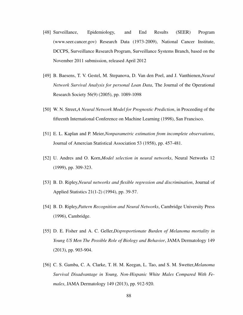
[48] Surveillance, Epidemiology, and End Results (SEER) Program

(www.seer.cancer.gov) Research Data (1973-2009), National Cancer Institute,

DCCPS, Surveillance Research Program, Surveillance Systems Branch, based on the

November 2011 submission, released April 2012

[49] B. Baesens, T. V. Gestel, M. Stepanova, D. Van den Poel, and J. Vanthienen,Neural

Network Survival Analysis for personal Loan Data, The Journal of the Operational

Research Society 56(9) (2005), pp. 1089-1098

[50] W. N. Street,A Neural Network Model for Prognostic Prediction, in Proceeding of the

fifteenth International Conference on Machine Learning (1998), San Francisco.

[51] E. L. Kaplan and P. Meier,Nonparametric estimation from incomplete observations,

Journal of Amercian Statistical Association 53 (1958), pp. 457-481.

[52] U. Andres and O. Korn,Model selection in neural networks, Neural Networks 12

(1999), pp. 309-323.

[53] B. D. Ripley,Neural networks and flexible regression and discrimination, Journal of

Applied Statistics 21(1-2) (1994), pp. 39-57.

[54] B. D. Ripley,Pattern Recognition and Neural Networks, Cambridge University Press

(1996), Cambridge.

[55] D. E. Fisher and A. C. Geller,Disproportionate Burden of Melanoma mortality in

Young US Men The Possible Role of Biology and Behavior, JAMA Dermatology 149

(2013), pp. 903-904.

[56] C. S. Gamba, C. A. Clarke, T. H. M. Keegan, L. Tao, and S. M. Swetter,Melanoma

Survival Disadvantage in Young, Non-Hispanic White Males Compared With Fe-

males, JAMA Dermatology 149 (2013), pp. 912-920.

88

[57] P. J. G. Lisboa, H. Wong, P. Harris, and R. Swindell,A Bayesian neural network ap-

proach for modeling censored data with an application to prognosis after surgery for

breast cancer, Artificial Intelligence in Medicine 28 (2003), pp. 1-25.

[58] Surveillance, Epidemiology, and End Results (SEER) Program

(www.seer.cancer.gov) Research Data (1973-2010), National Cancer Institute,

DCCPS, Surveillance Research Program, Surveillance Systems Branch, based on the

November 2012 submission, released April 2013

[59] E. M. Bignazoli, P. Boracchi, F. Ambrogi,and E. Marubini, Artificial neural network

for the joint modeling of discrete cause-specific hazards, Artificial Intelligence in

Medicine, 37(2) (2006),pp. 119-130.

[60] Paulo J. G. Lisboa, Terence A. Etchells, Ian H. Jarman, Corneliu T. C. Arsene, M. S.

Hane Aung, Antonio Eleuteri, Azzam F. G. Taktak, Federico Ambrogi, Patrizia Bo-

racchi, and Elia Biganzoli, Partial Logistic Artificial Neural Network for COmpeting

Risks Regularized With Automatic Relevance Determination, IEEE Transactions on

Neural Networks 20 (9) (2009), pp. 1403-1416

[61] John D. Kalbfleisch and Ross L. Prentice, The Statistical Analysis of Failure Time

Data, Second Edition, John Wiley & Sons (2002), Hoboken, New Jersey.

[62] Ian T. Nabney, NETLAB: Algorithms for Pattern Recognition, Springer-Verlag (2004),

London

[63] Frank E. Harrell Jr., Kerry L. Lee, and Daniel B. Mark, Tutorial in Biostatistics Mul-

tivariable Prognostic Models: Issues in Developing Models, Evaluating Assumptions

and Adequacy, and Measuring and Reducing Errors, Statistics in Medicine 15 (1996),

pp. 361-387

[64] Laura Antolini, Patrizia Boracchi, and Elia Biganzoli, A time-dependent discrimina-

tion index for survival data, Statistics in Medicine 24 (2005), pp. 3927-3944

89

[65] Elia Biganzoli, Patrizia Boracchi, and Ettore Marubini, A general framework for neu-

ral network models on censored survival data, Neural Networks 15(2) (2002), pp.

209-218

[66] Yongming Wang and Junzhong Gu, Comparative study among three different artificial

neural networks to infectious diarrhea forecasting, IEEE International Conference on

Bioinformatics and Biomedicine (2014), pp 40-46

[67] Mohammad Rasouli and Hamid Nikraz, Application of generalised regression neural

networks in trip distribution modelling, Road & Transport Research: A journal of

Australian and New Zealand Research and Practice 23 (3) (2014), pp. 13-25

[68] T. C. Wong and Alan H. S. Chan, A neural network-based methodol-

ogy of quantifying the association between the design variables and the

users’ performances, International Journal of Production Research (2014),

http://www.tandfonline.com/action/showCitFormats?doi=10.1080/00207543.2014.988886

[69] Z. O. Ojekunle, F. F. Oyebamji, A. O. Olatunde, O. R. Sangowusi, V. O. Ojejunle,

B. T. Amujo , and O. E. Dada, Global Climate Change: The Empirical Study of the

sensitivity Model in China’s Sustainable Development, part 2, Energy Sources, Part

A: Recovery, Utilization, and Environmental Effects 37 (8) (2015), pp. 861-869

[70] Y. Xu and C.P. Tsokos, Attributable Variables with Interactions that Contribute to

Carbon Dioxide in the Atmosphere, Frontiers in Science, 3(1) (2013), pp. 6-13.

[71] Jan Burck, Franziska Marten, and Christoph Bals, THe Climate Change Performance

Index Results 2015, GermanWatch - Berlin Office (2014)

[72] Mohammad H. Varzandeh, Omid Rahbari, Majid Vafaeipour, Kaamran Raahemifar,

and Fahime Heidarzade, Performance of Wavelet Neural Network and ANFIS Algo-

rithms for Short-Term Prediction of Solar Radiation and Wind Velocities, The 4th

World Sustainability Forum (2014)

90

[73] Xuezhong Guan, Ligang Sun, Fangfei Ui, and Xin Li, Sunspot Number Time Series

Prediction using Neural Networks with Quantum Gate Nodes, Proceeding of the 11th

World Congress on Intelligent Control and Automation (2014), Shenyang, China

[74] G. Zhang, B. Eddy Patuwo, and M. Hu,Forecasting with artificial neural networks:

The state of the art, International Journal of Forecasting 14 (1998), pp. 35-62

[75] Z. Tang and P. A. Fishwick, Feedforward neural nets as models for time series fore-

casting, ORSA Journal on Computing 5 (4) (1993), pp. 374-385

[76] H. F. Zou, G. P. Xia, F. T. Yang, and H. Y. Wang,An investigation and comparison

of artificial neural network and time series models for Chinese food grain price fore-

casting, Neurocomputing 70 (2007), pp. 2913-2923

[77] Juan P. Donate, X. Li, German G. Sanchez, and Araceli S. de Miguel, Time Series

forecasting by evolving artificial neural networks with genetic algorithms, differential

evolution and estimation of distribution algorithm, Neural Computing and Applica-

tions 22 (1) (2013), pp. 11-20

[78] S. N. Mandal, A. Ghosh. S. Roy, J. P. Choudhury, and S. R. Bhadra, A Novel Approach

of Genetic Algorithm in prediction of Time Series Data, Special Issue of International

Journal of Computer Applications (2012), pp. 16-20

[79] Ganji Huang and Lingzhi Wang,Hybrid Neural Network Models for Hydrologic Time

Series Forecasting Based on Genetic Algorithm, Fourth International Joint Confer-

ence on Computational Sciences and Optimization 147 (2011), pp. 1347 1350

[80] Vida Varahrami, Application of Genetic Algorithm to Neural Network Forecasting of

Short-Term Water Demand, International Conference on Applied Economics (2010),

pp. 783-787

91

[81] Jonathan L. Ticknor, A Bayesian regularized artificial neural network for stock market

forecasting, Expert Systems with Applications 40 (2013), pp. 5501-5506

[82] George EP Box, Gwilym M. Jenkins, Time series analysis: forecasting and control,

Holden-Day (1970), San Francisco CA.

[83] H. Akaike, Information theory and an extension of the maximum likelihood principle,

2nd International Symposium on Information Theory, Armenia, USSR (1971), pp.

267-281

[84] Dr. Pieter Tans, NOAA/ESRL (www.esrl.noaa.gov/gmd/ccgg/trends/) and Dr. Ralph

Keeling, Scripps Institution of Oceanography (scrippsco2.ucsd.edu/).

92