statistical and computational methods for differential
TRANSCRIPT

Statistical and Computational Methods for Differential
Expression Analysis in High-throughput Gene Expression Data
by
Yang Shi
A dissertation submitted in partial fulfillment
of the requirements for the degree of
Doctor of Philosophy
(Biostatistics)
in the University of Michigan
2016
Doctoral Committee:
Assistant Professor Hui Jiang, Co-Chair
Associate Professor Huining Kang, Co-Chair, University of New Mexico
Professor Ji-Hyun Lee, University of New Mexico
Associate Professor Maureen Sartor
Assistant Professor Xiaoquan William Wen

© Copyright by Yang Shi 2016
All Rights Reserved

ii
DEDICATION
To Dad and Mom, Yaping Shi and Xiaochun Yang,
Grandpa and Granny, Dinghan Shi and Quanquan Ding,
and
My Fiancée, Junqiushi Ren (Qiu-Qiu)
for their everlasting love, support and encouragement throughout my life.

iii
ACKNOWLEDEGMENTS
This dissertation is the result of five and half years of work in my doctoral study, where I have
been accompanied and supported by many people. I would like to express my sincere thanks to
everyone who has given me enthusiastic help and support during the past five and half years,
without which the completion of this dissertation is not possible.
I would like to thank my primary advisor, Dr. Hui Jiang, for his guidance, support and
encouragement during my Ph.D. study, and I feel it is difficult to express my deep gratitude to Hui
in a few sentences. I started to work with Hui from the summer of 2012, and I did not even know
to write a single line of R code at that time. Without Hui’s guidance, I cannot imagine that I can
arrive at this stage of the completion of this dissertation. I cherish my study under Hui’s guidance
during the past few years as the most valuable and important experience in my life, and it is my
greatest fortune to have Hui as my doctoral advisor.
I would like to thank my co-advisor, Dr. Huining Kang, for his help, encouragement and
suggestions during the second half of my Ph.D. study. Huining is always patiently listening to my
questions and offering helpful suggestions. I cannot forget the scene where Huining taught me how
to run parallel computing with R step by step on the computer clusters. Without Huining’s help, I
cannot imagine that the second part of this dissertation can be completed efficiently.
I would like to thank my committee member and primary supervisor at University of New
Mexico Comprehensive Cancer Center (UNMCCC), Dr. Ji-Hyun Lee, for her support,
encouragement and understanding. Ji-Hyun, many thanks for your help during my difficult
moments and offering me the opportunity to work at UNMCCC. I have learned and will keep

iv
learning from you not only the knowledge of statistics beyond my dissertation work, but also the
practice of being a professional biostatistician.
I would like to thank my committee members, Drs. Maureen Sartor and William Wen, for helpful
discussions with me and their valuable comments and useful suggestions on my dissertation
research, which have greatly improved the quality of this work. I would also like to thank Dr. Bin
Nan for being the procedure chair on my dissertation defense. Besides their dedicated service,
Maureen, William and Bin were also the instructors of three courses that I have taken in my
graduate study, and they are great teachers who have introduced me the knowledge of
bioinformatics methods, stochastic process and statistical inference.
I would like to thank my teachers and friends at University of Michigan, Ann Arbor. Many
thanks to my teachers, Drs. Douglas Schaubel, Min Zhang, Lu Wang, Thomas Braun, Michael
Boehnke, Peter Song and Brisa Sanchez, for teaching me the basic knowledge of statistics and
bringing me into the world of statistics. Many thanks to my dear friends, Qixing Liang, Sheng Qiu,
Yumeng Li, Tianyu Zhan, Jingchunzi Shi, Meng Xia, Yebin Tao, Teng Ming, Yilun Sun, Tzu-
Ying Liu, Xin Wang, Wenting Cheng, Lu Tang, Ken-Han Lin, Sophie Chen, Boxian Wei, Hai Shu,
Zihuai He, Zhe Fei, Vincent Tan, Xu Shu, Di Yang, Lei Yu, Xin Xin, Bao-Qui Tran, Sayantan
Das, Brian Segal, Paul Imbriano, Xiaoyan Zhang, Qiang Chen, Shijiao Huang, Chenghao Ma,
Leibin Wang (this is not a complete list) for their help and support during the past few years. I will
cherish the friendships and memories with all of you forever in my life. Many thanks to the
wonderful administrative team at the biostatistics department, Nicole Fenech, Fatma Nedjari,
Sabrina Clayton, Jamie Clay and Wendy Mashburn, who have given me a lot of help during my
graduate study.
I would like to thank my supervisors, collaborators and colleagues at UNMCCC. Many thanks
to Dr. Cheryl Willman for offering me the opportunity to work at UNMCCC, and Drs. Cosette
Wheeler and Marianne Berwick for providing me the financial support for my work at UNMCCC
from their research grants, and I cannot imagine that I can complete my Ph.D. study smoothly
without all of their support and understanding. Many thanks to my friends and colleagues at the
Biostatistics Shared Resource of UNMCCC, Ruofei Du, Tawny Boyce, Li Luo, Zhanna
Galochkina, Li Li, Herbert Davis, John Pesko and Davina Santillian for their invaluable help and

v
support in many different ways. I also would like to thank University of New Mexico Center for
Advanced Research Computing for computational resources used in this dissertation.
I would like to express my deep thanks to my parents, Yaping Shi and Xiaochun Yang, and my
grandparents, Dinghan Shi and Quanquan Ding, for their everlasting love, support and
encouragement throughout my life. Finally, to my beloved fiancée, Qiu-Qiu, many thanks for not
appearing during the first three and half years of my Ph.D. study so that I could concentrate on my
research work, and it is much more than a simple thank you for your arrival in my life in the
summer of the year 2015, as the most valuable gift from Heaven and right on the time when I
needed your love and company to continue the journey of life.

vi
TABLE OF CONTENTS
DEDICATION ............................................................................................................................... ii
ACKNOWLEDEGMENTS ........................................................................................................ iii
LIST OF FIGURES ..................................................................................................................... ix
LIST OF TABLES ........................................................................................................................ xi
CHAPTER
I. Introduction ............................................................................................................................... 1
1.1 Overview .......................................................................................................................... 1
1.2 Differential expression analysis in high-throughput gene expression data ............... 2
1.3 Dissertation outline ......................................................................................................... 4
II. rSeqDiff: Detecting Differential Isoform Expression from RNA-Seq Data using
Hierarchical Likelihood Ratio Test ............................................................................................. 7
2.1 Introduction ..................................................................................................................... 7
2.2 Methods ............................................................................................................................ 8
2.2.1 Notations ................................................................................................................ 9
2.2.2 The linear Poisson model for multi-sample RNA-Seq data ................................... 9
2.2.3 Model selection using hierarchical likelihood ratio test ...................................... 13
2.2.4 Ranking of differentially spliced genes ............................................................... 14
2.3 Results ............................................................................................................................ 14
2.3.1 Simulation studies ................................................................................................ 15
2.3.2 Applications of rSeqDiff to real RNA-Seq datasets ............................................ 15

vii
2.4 Discussion....................................................................................................................... 25
III. rSeqNP: A Non-parametric Approach for Detecting Gene Differential Expression and
Splicing from RNA-Seq Data ..................................................................................................... 27
3.1 Introduction ................................................................................................................... 27
3.2 Methods .......................................................................................................................... 28
3.2.1 Data preprocessing ............................................................................................... 28
3.2.2 Testing Differential Expression of genes and isoforms ....................................... 28
3.2.3 Testing Differential Expression and Splicing of genes jointly............................. 32
3.3 Simulation studies ......................................................................................................... 33
3.3.1 Direct simulation of expression values ................................................................ 33
3.3.2 Simulation of RNA-Seq reads ............................................................................. 35
3.4 Application to a prostate cancer RNA-Seq dataset .................................................... 41
IV. A Two-part Mixed Model for Differential Expression Analysis in Single-cell High-
throughput Gene Expression Data ............................................................................................ 47
4.1 Introduction ................................................................................................................... 47
4.2 Methods .......................................................................................................................... 48
4.2.1 The two-part mixed model for single-cell gene expression data ......................... 48
4.2.3 Testing for differential expression ....................................................................... 52
4.3 Simulation studies ......................................................................................................... 54
4.3.1 Evaluation of type I error rates ............................................................................ 54
4.3.2 Evaluation of statistical power ............................................................................. 60
4.4 Application to real single cell gene expression data ....................................................... 63
4.4.1 Application to a scRT-PCR dataset ...................................................................... 63
4.4.2 Application to a scRNA-Seq dataset .................................................................... 67
4.5 Discussion ....................................................................................................................... 68
V. Efficient estimation of small p-values in permutation tests using importance sampling
and cross-entropy method .......................................................................................................... 73
5.1 Introduction ................................................................................................................... 73
5.2 Introduction of the adaptive CE method .................................................................... 75
viii
5.2.1 Monte Carlo simulation and importance sampling .............................................. 75
5.2.2 The adaptive CE method ...................................................................................... 76
5.3 Estimating small p-values for permutation tests using the adaptive CE method ... 78
5.3.1 Permutation test for paired two-group data ......................................................... 79
5.3.2 Permutation test for unpaired two-group data ..................................................... 81
5.4 Results ............................................................................................................................ 86
5.4.1 Simulation studies for unpaired two-group permutation test ............................... 86
5.4.2 Application to a microarray gene expression study ............................................. 88
5.5 Discussion and future work .......................................................................................... 88
VI. Efficient estimation of small p-values in parametric bootstrap tests using Hamiltonian
Monte Carlo cross-entropy method ........................................................................................... 94
6.1 Introduction ................................................................................................................... 94
6.2 Methods .......................................................................................................................... 96
6.2.1 Estimating small parametric bootstrap p-values using cross-entropy method ..... 96
6.2.2 Limitations of the adaptive CE method ............................................................... 98
6.2.3 Sampling from the optimal proposal density ....................................................... 99
6.3 Application: parametric bootstrap tests for variance components in LMMs ....... 103
6.3.1 Test the variance component for LMMs with a single variance component ..... 105
6.3.2 Test one variance component in LMMs with multiple variance components ... 108
6.3.3 Application to gene set differential expression analysis ..................................... 111
6.4 Discussion......................................................................................................................115
VII. Summary and Discussion ..................................................................................................116
7.1 Statistical methods for differential expression analysis ............................................116
7.2 Resampling methods, Monte Carlo simulation and the cross-entropy method .....117
APPENDIX .................................................................................................................................119
BIBLIOGRAPHY ..................................................................................................................... 136

ix
LIST OF FIGURES
Figure 2.1 Illustration of the three models. ................................................................................... 12
Figure 2.2 Models for estimating the exon inclusion level ψ using the junction reads. ............... 18
Figure 2.3 Comparisons of rSeqDiff, MATS, Cuffdiff 2 and RT-PCR assays. ............................. 19
Figure 2.4 Examples comparing the estimates between rSeqDiff, MATS, Cuffdiff 2 and RT-PCR
assays. ........................................................................................................................................... 21
Figure 2.5 Examples demonstrating the estimates from rSeqDiff. ............................................... 25
Figure 3.1 ROC curves of different testing methods in each scenario of the simulations. ........... 39
Figure 3.2 Comparison of quantification results of isoform expression by rSeq, RSEM and Cuffdiff.
....................................................................................................................................................... 42
Figure 3.3 Comparison of the permutation test based on the GDS with Wilcoxon rank-sum test
(WRS) and Wilcoxon signed-rank test (WSR). ............................................................................ 44
Figure 3.4 Two individual gene examples to demonstrate the strength of the paired two-group
comparison and the permutation test based on the GDS. ............................................................. 45
Figure 4.1 Plots of the observed versus the expected p-values for the Wald test for the Gaussian
part under H0: no significant difference between the two conditions. .......................................... 56
Figure 4.2 Plots of the observed versus the expected p-values for the Wald test for the binomial
part under H0: no significant difference between the two conditions. .......................................... 57

x
Figure 4.3 Plots of the observed versus the expected p-values for the likelihood ratio test for the
Gaussian part under H0: no significant difference between the two conditions. .......................... 58
Figure 4.4 Plots of the observed versus the expected p-values for the likelihood ratio test for the
binomial part under H0: no significant difference between the two conditions. ........................... 59
Figure 4.5 Plots of the observed versus the expected p-values for jointly testing the Gaussian and
binomial parts under H0: no significant difference between the two conditions. ......................... 60
Figure 4.6 Comparisons of statistical powers of different methods. ............................................ 62
Figure 4.7 Comparisons of the p-values from TMM and MAST for the scRT-PCR dataset. ...... 65
Figure 4.8 Number of differentially expressed genes identified by each method with FDR<0.01.
....................................................................................................................................................... 68
Figure A.1 The analysis pipeline of rSeqDiff. ............................................................................ 125
Figure A.2 A hypothetical gene used in the simulations. ........................................................... 126
Figure A.3 Scatter plots for examing differential expression and differential splicing. ............. 133
Figure A.4 Comparison between rSeqDiff and Cuffdiff 2 with the ASD dataset. ...................... 134

xi
LIST OF TABLES
Table 2.1 Summary of notations ..................................................................................................... 9
Table 2.2 Summary of hLRT for model selection ........................................................................ 14
Table 2.3 The correlation coefficients of the values between RT-PCR and rSeqDiff, MATS
and Cuffdiff 2 for the 164 RT-PCR tested exons .......................................................................... 17
Table 2.4 Ranking of RT-PCR validated genes with relevant neurological functions ................. 23
Table 3.1 Non-parametric statistics used by rSeqNP .................................................................... 29
Table 3.2 Notations in the Methods Section ................................................................................. 29
Table 3.3 Summary of type I error rate......................................................................................... 34
Table 3.4 Summary of statistical power ....................................................................................... 35
Table 3.5 FDP, type I error rate, power and AUC of different testing methods in each scenario in
the simulations .............................................................................................................................. 40
Table 3.6 Numbers of genes identified by different programs from the prostate cancer RNA-Seq
dataset ........................................................................................................................................... 44
Table 3.7 Number of differential genes identified by rSeqNP without filtering noisy genes in the
prostate cancer RNA-Seq dataset.................................................................................................. 46
Table 4.1 Results of the gene differential expression analysis for the HIV scRT-PCR dataset. ... 69

xii
Table 4.2 P-values and FDR for the top 20 differentially expressed genes. ................................. 72
Table 5.1 Performance of different algorithms on the first two-group permutation test example.
....................................................................................................................................................... 90
Table 5.2 Performance of different algorithms on the second two-group permutation test example.
....................................................................................................................................................... 91
Table 5.3 Estimated exact p-values for the top 23 probe sets of the MRD data. .......................... 92
Table 6.1 Simulation results of parametric bootstrap tests for variance component in LMMs with
a single random effect – varying effect size. .............................................................................. 107
Table 6.2 Simulation results of parametric bootstrap tests for variance component in LMMs with
a single random effect – varying sample size. ............................................................................ 108
Table 6.3 Simulation results of parametric bootstrap tests for one variance component in LMMs
with multiple variance components ............................................................................................ 111
Table 6.4 Estimated p-values for the top 14 differentially expressed gene sets ......................... 113
Table A.1 Summary of true classification rate under model 0 ................................................... 127
Table A.2 Summary of true classification rate under model 1 ................................................... 128
Table A.3 Summary of true classification rate under model 2 ................................................... 129
Table A.4 Comparison of differential spliced genes across biological replicates in the ASD dataset
..................................................................................................................................................... 135
Table A.5 Comparison of the estimated differentially used exon inclusion levels for the five RT-
PCR validated genes between rSeqDiff and the exon-based method ......................................... 135

1
CHAPTER I
Introduction
1.1 Overview
High-throughput gene expression profiling technologies such as microarray, RNA-Sequencing
(RNA-Seq) and parallel real-time polymerase chain reaction (RT-PCR) have revolutionized the
study of gene expression and function and opened a new era in biology [1-5]. These methods can
simultaneously measure the expression levels of hundreds to tens of thousands of genes in different
biological samples and can provide global insights for understanding the associations between
gene expression and complex biological processes [1].
The microarray technology, debuted in late 1990s [6], has become a regular and standard tool
for genomic research [1,5]. The principle of this technology involves the hybridization of
fluorescently labelled cDNAs with synthetic DNA probes on custom-designed chips, and the gene
expression levels are measured by the florescence signals of the probes [2,5]. Despite its
limitations compared with the most recent RNA-Seq technology such as high background noise
due to cross-hybridization and the limited range of the detection of gene expression due to both
background noise and signal saturation [2], microarray is still an important tool for gene expression
analysis [1,5] and has enabled researchers to conduct large-scale studies to identify the associations
between gene expression and diseases in humans [7,8] at a relative low cost.
As an alternative to microarray, the RNA-Seq technology has rapidly evolved as a powerful and
widely-used tool for gene expression studies [2,3,9] since its debut in biomedical research in the
late 2000s [10-13]. RNA-Seq uses the technology of massive parallel sequencing (next generation
sequencing, NGS) to sequence the cDNAs that are reverse-transcribed from RNAs of different
biological samples, and generates millions of short reads [2,3,10]. These reads are aligned to the

2
reference genome and the number of reads mapped to a certain region on the genome of interest
(called the genomic feature, such as gene, exon or isoform) are summarized and used to measure
the abundance of the genomic feature in the biological sample [3,14,15]. Compared with
microarray, RNA-Seq not only has the advantages of lower background noise and broader range
of gene expression measure [16], but also can be used to detect new transcripts through de novo
transcriptome reconstruction, to perform differential expression analysis for alternative spliced
isoforms and to estimate allele-specific expression [1-3,9,16,17].
1.2 Differential expression analysis in high-throughput gene expression data
Differential expression analysis, which refers to the identification of genomic features that are
significantly different in abundance between distinct groups of biological samples (these groups
are called biological conditions) or significantly associated with a given outcome or response
variable [15,18,19], is one of the most important goals in high-throughput gene expression studies
[19].
In general, most of the current statistical methods used for differential expression analysis in
high-throughput gene expression data can be classified into two groups: parametric methods and
non-parametric methods. The parametric methods have distributional assumptions for the gene
expression data. For microarray data, the florescence intensities are often treated as continuous
variables and gene expression values are commonly assumed to follow a log-normal distribution
after proper normalizations and background noise subtraction [5,20]. Therefore, the linear-model
based methods are widely used for modelling microarray gene expression data [5,20], and the
limma package [20] is one well-known method among them. For a comprehensive review of other
types of statistical methods used in microarray analysis, see [5]. For RNA-Seq, the nature of the
gene expression data are the counts of short reads mapped to genomic features, therefore statistical
models for count data, such as Poisson [9,21] or negative binomial regression models [22-24], are
proposed to model RNA-Seq data. In addition to the count-based modelling approaches, other
researchers have proposed to first apply transformations to the read count data from RNA-Seq to
make the data to be continuous and roughly follow the log-normal distribution, then apply the
linear-model based methods developed for microarray data analysis to RNA-Seq data [25,26]. A

3
list of software tools for differential expression analysis in RNA-Seq are given in Chapter 8 of [3]
and comparisons of different methods can be found in [15,18].
As alternatives to the parametric methods discussed above, non-parametric approaches also
have been developed and used for differential expression analysis with both microarrays [27] and
RNA-Seq data [14,28-30]. For those non-parametric methods, a summary statistic is computed as
the test statistic based on the gene expression data, and then resampling based methods such as
permutation [14,27,28,30] or bootstrap [29] are used to estimate the empirical distribution of the
test statistic under the null hypothesis that there is no differential expression between biological
conditions. Compared with parametric approaches, non-parametric methods do not have the
relative strong distributional assumptions for the gene expression data and therefore are more
robust when the distributional assumptions of the parametric approaches are violated and outliers
exist in the data [14,28,29]. In fact, some researchers argue that in large sample size RNA-Seq
experiments where the variations between biological samples tend to be large and outliers (one
sample has a large number of read counts for a particular gene) often present, the assumed
distributions of the parametric approaches tend to be violated, and as a consequence the results of
those parametric approaches are not reliable [14].
On the other hand, the parametric approaches are more efficient and powerful for testing
differential expression than the non-parametric methods when the assumed distribution is a good
approximation of the gene expression data [14,15,22,23]. Furthermore, adjusting confounding
variables can be easily achieved in parametric regression models [20,22,23,26], but is not
straightforward in those non-parametric methods. Lastly but importantly, usually a large number
of resamples is needed for obtaining reliable estimations of small p-values for those resampling-
based non-parametric approaches [27,31], which requires intensive computational efforts.
Therefore, non-parametric approaches usually take longer computational time than parametric
methods.
In recent years, RNA-Seq has also been widely used for the study of alternative splicing in
humans and model organisms [10,11,16,32], and the detection of differential splicing from RNA-
Seq is an important research direction. Several statistical approaches have been proposed towards
this end. One type of those approaches is exon-based, which focuses on the detection of differential
usage of exons, such as DEXSeq [33], rMATS[34], DSGseq[35], and SplicingCompass[36]. The

4
other type of those approaches is isoform-based, which focuses on the detection of differential
expression of isoforms across different biological conditions, such as Cufflinks/Cuffdiff 2 [37],
rDiff-parametric [38], BitSeq [39] and EBSeq [40]. Comparisons of some of those methods can
be found in [41]. It should be noted that the aforementioned methods are all based on known
isoform annotations. More recently, methods that enable the detection of differential usage of
novel exons and splice junctions have also been developed, and one notable method is JunctionSeq
[42], which can be applied to the scenario where the alternatively spliced isoforms are not
annotated [42].
Despite the significant progress in the development of statistical methodologies and
bioinformatics tools for the analysis of high-throughput gene expression data, there is still a
growing need for novel statistical methods and efficient computational algorithms. One reason is
that new types of data and complex study designs emerge as the technology continue to evolve.
As a highlighted example, single-cell RNA-seq (scRNA-seq), which enables researchers to
examine mRNA expression at the resolution of individual cells, is a novel technology attracting
considerate attention these days [43-46]. Compared with regular RNA-Seq experiments, scRNA-
seq usually has a much larger number of samples from individual cells and the gene expression
data from scRNA-seq show notable distinct features, such as excessive zero expression values and
high variability across samples [43,45]. Therefore, many statistical methods developed for regular
RNA-Seq data analysis cannot be directly applied for scRNA-seq data. In summary, we can
foresee that high-throughput gene expression profiling technologies will still be fast-growing in
future years and large amounts of different types of data will be generated, which brings both
opportunities and challenges for biologists, bioinformaticians and statisticians.
1.3 Dissertation outline
The aim of this dissertation is to develop novel statistical and computational methods for
differential expression analysis in high-throughput gene expression data.
In the first part of this dissertation, we develop statistical models for differential expression
analysis with a variety of study designs, and this part contains three research projects, which are
presented in Chapter II, III and IV respectively. In Chapter II, we present an efficient algorithm
for the detection of differential expression and differential splicing of genes in RNA-Seq data. Our

5
approach considers three cases for each gene: 1) no differential expression, 2) differential
expression without differential splicing and 3) differential splicing. We use a Poisson regression
framework to model the read counts and use a hierarchical likelihood ratio test approach for model
selection. Simulation studies show that our approach achieves good power for detecting
differentially expressed or differentially spliced genes, and comparisons with competing methods
on two real RNA-Seq datasets demonstrate that our approach provides accurate estimates of
isoform abundances and biological meaningful rankings of differentially spliced genes.
In Chapter III, we present a non-parametric approach for the joint detection of differential
expression and differential splicing of genes. We introduce a new statistic named gene-level
differential score and use a permutation test to assess the statistical significance. The method can
be applied to datasets with a variety of experimental designs, including those with two (unpaired
or paired) or multiple biological conditions, and those with quantitative or survival outcomes.
In Chapter IV, we model single-cell gene expression data using a two-part mixed model. This
model not only adequately accounts for the distinct features of single cell expression data,
including extra zero expression values, high variability and clustered design, but also provides the
flexibility of adjusting for covariates. An efficient computational algorithm, automatic
differentiation, is used for estimating the model parameters. Comparisons with existing methods
through simulation studies and application to real single-cell gene expression data, our approach
achieves improved power for detecting differentially expressed genes.
In the second part of this dissertation, we propose novel methods to improve the computational
efficiency of resampling-based test methods in genomic studies with focus on differential
expression analysis, and this part contains two research projects, which are presented in Chapter
V and VI respectively. In Chapter V, we propose a fast algorithm for evaluating small p-values
from permutation tests based on an adaptive importance sampling approach, which uses the cross-
entropy method for finding the optimal proposal density. In Chapter VI, we develop an algorithm
for efficient estimation of small p-values in parametric bootstrap tests, which not only uses the
principle of the cross-entropy method to approximate the optimal proposal density, but also
incorporates the Hamiltonian Monte Carlo method to efficiently sample from the optimal proposal
density. Together, these methods address a critical challenge for resampling-based test methods in
genomic studies since usually an enormous number of resamples is needed for estimating very

6
small p-values. Simulation studies and applications to real gene expression datasets demonstrate
that our methods achieve significant gains in computational efficiency compared with existing
methods.

7
CHAPTER II
rSeqDiff: Detecting Differential Isoform Expression from RNA-Seq Data using
Hierarchical Likelihood Ratio Test
High-throughput sequencing of transcriptomes (RNA-Seq) has recently become a powerful
tool for the study of gene expression. In this chapter, we present an efficient algorithm for the
detection of differential expression and differential splicing of genes from RNA-Seq experiments
across multiple conditions. Unlike existing approaches which detect differential expression of
transcripts, our approach considers three cases for each gene: 1) no differential expression, 2)
differential expression without differential splicing and 3) differential splicing. We specify
statistical models characterizing each of these three cases and use hierarchical likelihood ratio test
for model selection. Simulation studies show that our approach achieves good power for detecting
differentially expressed or differentially spliced genes. Comparisons with competing methods on
two real RNA-Seq datasets demonstrate that our approach provides accurate estimates of isoform
abundances and biological meaningful rankings of differentially spliced genes. The proposed
approach is implemented as an R package named rSeqDiff, which is available at http://www-
personal.umich.edu/~jianghui/rseqdiff/. The content of this chapter has been published previously
in the journal PLOS ONE [47].
2.1 Introduction
Alternative splicing is an important mechanism in post-transcriptional regulation of eukaryotes.
Through alternative splicing, a single gene can produce multiple different transcript isoforms that
usually lead to different protein isoforms with different structures and biological functions, which
can greatly enrich the diversity of eukaryote transcriptomes [10,11,16]. Several studies also show
that many human disease-causing mutations affect alternative splicing rather than directly

8
affecting coding sequences and ill-regulated alternative splicing events have been implicated in a
large number of human pathologies [48-50]. Due to its vital role in biological processes such as
gene regulation, cell differentiation, development and disease pathophysiology, there is an urgent
need for the development of new technologies and methodologies for the study of alternative
splicing events and the quantification of the expression of alternative isoforms.
In recent years, high-throughput sequencing of transcriptomes (RNA-Seq) has rapidly evolved
as a powerful tool for the study of alternative splicing in humans and model organisms
[10,11,16,32]. Many RNA-Seq experiments have been conducted to investigate the following two
problems: (i) the discovery of novel transcripts and (ii) the estimation and detection of
differentially expressed transcripts. Here we focus on the second problem. Several statistical
approaches have been proposed in recent years towards this end. One type of approach is exon-
based, which focuses on the detection of differential usage of exons [17,33,51,52]. The other type
of approach is isoform-based, which focuses on the estimation of differential expression of
isoforms across different biological conditions [37,39,53-55].
In this chapter, we present an isoform-based approach for the detection of differential isoform
expression from multiple RNA-Seq samples. In particular, we extend the linear Poisson model in
[9,56] for the estimation of isoform abundances from single-end or paired-end RNA-Seq data.
Unlike existing approaches which detect differential expression of transcripts, we consider three
cases for each gene: 1) no differential expression, 2) differential expression without differential
splicing and 3) differential splicing. We specify statistical models characterizing each of these three
cases and use hierarchical likelihood ratio test for model selection. The remaining part of the
chapter is organized as follows: We first introduce the statistical model and method, and then use
simulations to study the type-I error and statistical power of the proposed method, followed by the
analyses of two real RNA-Seq datasets. For the first dataset (an ESRP1 dataset published in [52]),
we compare our approach with two other methods (MATS [52] and Cuffdiff 2 [37]) using RT-PCR
assays performed in [52]. For the second dataset (an ASD dataset published in [57]), we present a
genome-widely analysis of differential splicing between Autism Spectrum Disorder (ASD) and
normal brain samples.
2.2 Methods

9
2.2.1 Notations
We use similar notations as in [56] to present the statistical model, which are summarized in
Table 2.1 and explained in details below.
Table 2.1 Summary of notations
Symbol Meaning
Total number of biological conditions in the study.
Total number of transcripts (isoforms) of a specific gene of interest.
Total number of read types in the kth condition (we write Jk as J to avoid
cluttering, but note this quantity depends on the condition k).
The I×Jk read sampling rate matrix for the kth condition.
The Jk×1 read count vector for the kth condition.
The K×I isoform abundance matrix for all K conditions. The kth row corresponds
to the isoform abundance vector for the kth condition.
The I×1 joint isoform abundance vector for all K conditions (for model 0 only).
1 The I×1 basic isoform abundance vector (for model 1 only).
The K×1 isoform ratio vector (for model 1 only).
The kth element of τ which is the ratio between the isoform abundance vector for
the kth condition and the basic isoform abundance vector, i.e. =τk 1 (for model
1 only).
The likelihood functions for model 0, 1 and 2 (l0, l1 and l2 are the log-likelihood
for each model), respectively.
2.2.2 The linear Poisson model for multi-sample RNA-Seq data
We extend the linear Poisson model for one-sample RNA-Seq data in [9,56] to multiple samples.
Assume there are K conditions in the study, and in the kth condition there are Jk distinct read types.
A read type refers to a group of reads (single-end or paired-end) mapped to same position in a
K
I
( )kJ J
kA
kN
0
k
k
0 1 2, ,L L L

10
transcript [56]. We write Jk as J to avoid cluttering but note this quantity depends on the condition
k. For a gene G of interest with I annotated transcripts (isoforms), we define θ as the K×I isoform
abundance matrix for all the K conditions, where the kth row vector of this matrix,
1, 2, , T
k k k kI denotes the isoform abundance vector of G in the kth condition, and ki
denotes the abundance of the ith isoform in the kth condition. Correspondingly, each condition has
its own read sampling rate matrix
11 1
1
k k J
k
kI kIJ
a a
A
a a
where kija denotes the rate that read type j is sampled from isoform i in condition k. In our
implementation we adopt the uniform sampling model in [56] for single-end reads which assumes
all the possible read types from a transcript are generated with the same rate. For paired-end reads
we adopt the insert length model in [56], which assumes the sampling rate of a particular paired-
end read type depends on its insert size. The sampling rate matrix Ak can be estimated based on all
the mapped reads in condition k [56]. Each condition also has its own read count vector
1 2, , , T
k k k kJN n n n , where nkj denotes the number of reads of type j mapped to any of the I
isoforms in condition k. Given k and Ak, Nk is assumed to follow the one-sample linear Poisson
model [9,56]. In particular, the probability mass function of Nk is
·
1
·
!
kj k kj
k
n aJ
k kj
k
j kj
a ef N
n (2.1)
where 1
·
I
k kj ki kij
i
a a .
Given Ak and Nk for k=1,…,K, our goal is to jointly estimate θ combining the data from all the
samples. This will be complicated by the fact that the k ’s may not be independent of each other
under different biological situations. Therefore, we need to re-parameterize θ according to the
underlying biological situation of whether the gene and its isoforms show differential expression.
In particular, we propose the following three nested models (Figure 2.1) corresponding to three
possible underlying biological situations regarding the pattern of gene expression across multiple

11
conditions.
Model 0 [no differential expression] characterizes the situation where none of the gene’s isoforms
show differential expression across the K conditions (Figure 2.1B, row 1, where the hypothetical
gene structure is given in Figure 2.1A). Under this model, all K conditions have the same isoform
expression levels so that all the rows of θ are the same and equal to a joint isoform abundance
vector 0 k , k=1, 2, … K. Under the assumption that the reads of each condition are generated
independently, the joint likelihood function of 0 combining all K conditions is the product of the
likelihood of each condition
0
0
·
0
0 0 1 2
1 1 1
·| , , ,
!
kjkj
n aK K J
kj
k k
k k j kj
a eL N N N f N
n (2.2)
Model 1 [differential expression without differential splicing] characterizes the situation where
the gene shows differential expression, but not differential splicing of its isoforms across the K
conditions (Figure 2.1B, row 2). Under this model, the relative abundances between the isoforms
are the same across the K conditions and the rows of θ are therefore proportional to each other.
Accordingly, we re-parameterize θ as the outer product of a K×1 vector τ and an I×1 vector 1 ,
where 1 is the basic isoform abundance vector for all K conditions, and τ is the isoform ratio
vector. To make the model identifiable, τ is subject to a linear constraint: 1 1|| || 1
K
kk
. For
the example of model 1 in Figure 2.1B, 1 [90,60] T and
1 2[ , ]3 3
T . If 1 2
1 K
K ,
model 1 degenerates to model 0. Similarly, the joint likelihood function of 1 and τ combining all
K conditions is
1
1
( )
1
1 1 1 2 ,1 1 1
[( ),, ,
]|
!,
kj k kj
k
n aK K Jk kj
K k
k k j kj
a eL N N N f N
n (2.3)
Model 2 [differential splicing] characterizes the situation where the gene shows differential
isoform usage across the K conditions (Figure 2.1B, row 3). Under this model, each condition has
its own independent isoform abundance vector k . Therefore, the joint likelihood function is

12
2 1 2 2 1 2 1 2
1
·
1 1
| , , , | ,
·
!
, , , , ,
k
kj k kj
K K K
K
k
k
n aK J
k kj
k j kj
L N N N L N N N
f N
a e
n
(2.4)
Figure 2.1 Illustration of the three models.
(A) A hypothetical gene with three exons and two isoforms in blue and red, respectively. (B) Three
models characterizing three biological situations of the gene expression patterns between two
conditions. The numbers of red and blue bars represent the relative abundances of the
corresponding isoforms in the two conditions.
The parameters of each of the three models can be estimated using maximum-likelihood

13
estimation (MLE). As discussed in [56], one computational burden in solving the MLE is that J
could be quite large, especially for paired-end RNA-Seq data. We adopt the two data reduction
techniques introduced in [56]: (i) We take only read types with non-zero mapped reads and further
group them to form larger read categories; (ii) For each condition k, we compute the total sampling
rate for each isoform i as1
J
kij
d
j
ef
kiw a
(denote 1 2, ,
T
k k k kJW w w w as the total sampling rate
vector for all isoforms) without enumerating each particular sampling rate kija . In practice, we
work with the reduced form of the likelihood functions for the three models, and the details of
these data reduction techniques are given in Appendix Section A.1.
Similar to the log-likelihood function for one-sample linear Poisson model given in equation (2.1)
(see also [9,56]), all the log-likelihood functions for the above three models are concave. Therefore,
the MLEs for all of the three models can be obtained by linear constraint convex optimization
algorithms. In practice, we use an expectation-maximization (EM) algorithm to calculate the
MLEs, and the details of the algorithm are given in Appendix Section A.1.
2.2.3 Model selection using hierarchical likelihood ratio test
Since model 0 is nested within model 1, which is again nested within model 2, we use the
likelihood ratio test (LRT) for model selection. For large sample size, the LRT statistics for nested
models asymptotically follow χ2 distributions. The degrees of freedom (DF) of the three models
are DF(model 0)=I (the free parameters are the I×1 joint isoform abundance vector 0 ), DF(model
1)=I+K-1 (the free parameters are the I×1 basic isoform abundance vector 1 and the K×1 isoform
abundance ratio vector τ subjects to one linear constraint 1
1
K
kk) and DF(model 2)=K×I (the
free parameters are the K×I isoform abundance matrix θ), respectively.
Given a pre-specified significance level α (e.g., 0.05), we perform model selection using the
following hierarchical likelihood ratio test (hLRT) procedure (Table 2.2). The first round tests
include two parallel tests which compare model 0 vs. model 1 and model 0 vs. model 2, each at
significance level α/2. If neither of the two tests is significant, then model 0 is selected. If only one
of the two tests is significant, model 1 or model 2 is selected accordingly. If both tests are
significant, we perform the second round test which compares model 1 vs. model 2 at significance

14
level α and selects model 2 if this test is significant or model 1 otherwise.
Table 2.2 Summary of hLRT for model selection
models being compared LRT statistics test against
first round tests
model 0 vs. model 1 , 1-α/2
model 0 vs. model 2 , 1-α/2
second round test model 1 vs. model 2 , 1-α
2.2.4 Ranking of differentially spliced genes
When comparing between two biological conditions (e.g., normal vs. diseased), it is often useful
to generate a ranking of genes being differentially spliced (i.e., model 2 genes). We rank model 2
genes as follows: Suppose 1̂ and 2̂ are the estimated isoform abundance vectors for the two
conditions, we calculate the statistic:
1 2
1 1
1
2 1
ˆ ˆ
ˆ ˆ||
1
|2 | | || || || |T
,
where ||·||1 denotes the vector L1 norm ([58] uses a similar statistic without the constant 1/2, which
is introduced here to have 0 1T ). Large T values indicate high level of differential splicing.
The T value is 0 for model 0 and model 1 genes. Alternatively, genes classified in model 1 or model
2 can also be ranked according to their p-values from the hLRT, if statistical significance is of
major interest.
The proposed approach is implemented as an R package named rSeqDiff, which is available at
http://www-personal.umich.edu/~jianghui/rseqdiff/. The analysis pipeline of using rSeqDiff is
provided in Appendix Section A.1.
2.3 Results
0 12 l l2
1 DF K
0 22 l l 2
( 1) DF K I
1 22 l l 2
( 1) ( 1) DF K I

15
2.3.1 Simulation studies
We study the performance of our proposed hLRT approach by simulating read counts from genes
with a wide range of abundances (from lowly expressed genes to highly expressed genes) and
report the specificity and sensitivity of our approach for the detection of differential expression
and differential splicing events. Detailed procedure and results of the simulation studies are given
in Appendix Section A.3, and here we briefly outline the methods that we applied in the simulations.
We test differential expression and differential splicing of a hypothetical gene with a well-
annotated known isoform structure (Figure A.2) between two biological conditions with
sequencing depths of total 50 million and 55 million reads, respectively. The gene structure and
the sequencing depths are fixed in the simulations. For each of the three models, we vary the
expression level (denoted as G in Appendix Section A.3) of the gene within a broad range, and for
each G we simulate the number of reads mapped to each of the two isoforms according to the three
models [equations (2.2), (2.3) and (2.4)]. For each G, we simulate 1000 replicated pairs of samples.
We run the hLRT with significance level α=0.05 using rSeqDiff on the 1000 simulated pairs of
samples and report the proportions of the simulated pairs of samples for which our approach
correctly selects the true underlying model (i.e., true classification rate). Table A.1, A.2 and A.3 in
Appendix show the true classification rates under model 0, 1 and 2, respectively.
In summary, the simulation studies show that our proposed hLRT approach has well controlled
type I error rate at α=0.05 (Table A.1 in Appendix) and good statistical power for detecting
differential expression and differential splicing for genes with moderate to high abundance in both
conditions (Table A.2 and A.3 in Appendix). When the gene is lowly expressed in one condition
but moderately or highly expressed in the other condition, our proposed hLRT approach still has
good power in selecting model 1, i.e., differential expression without differential splicing. The
power in detecting differential expression or differential splicing is low when the gene has low
expression levels in both conditions, which is well expected. In real data analysis, genes with very
low expression levels in all the conditions are usually filtered out prior to the analysis. By default,
rSeqDiff filters out genes with less than 5 reads in all the conditions.
2.3.2 Applications of rSeqDiff to real RNA-Seq datasets
We demonstrate the practical usage of rSeqDiff and compare it with two other approaches by

16
analyzing two real RNA-Seq datasets: the ESRP1 dataset and the ASD dataset.
Analysis of the ESRP1 dataset
Epithelial splicing Regulatory Protein 1 (ESRP1) is a master cell-type specific regulator of
alternative splicing that controls a global epithelial-specific splicing network [52]. This dataset
was published in [52], where Shen et al performed single-end RNA-Seq experiments on the MDA-
MB-231 cell line with ectopic expression of the ESRP1 gene and an empty vector (EV) as control.
The dataset contains 136 million reads for the ESRP1 sample and 120 million reads for the EV
sample. Shen et al used this dataset to demonstrate their exon-based approach MATS for detect
differential splicing, and performed RT-PCR assays to test for 164 exons skipping events. Since
the biological significance of this dataset was further analyzed in a follow-up paper by Shen and
collaborators [59], our analysis here is solely focused on the validation and comparisons of our
proposed hLRT approach with other methods using the 164 RT-PCR tested alternative exons as
gold standard.
MATS is an exon-based method and its results cannot be directly compared with our isoform-
based approach. In the MATS model (Figure 2.2A, modified from [52]), exon 2 is the alternatively
spliced exon (skipped exon) unique for the longer isoform and exon 1 and 3 are common exons
shared by both of the two isoforms. The exon inclusion level of the skipped exon was defined
as the abundance ratio between the longer isoform and the sum of both the two isoforms, which
was estimated as ( ) / 2
( ) / 2
UJC DJC
UJC DJC SJC
by MATS (Figure 2.2A). The exon inclusion level
difference between the two conditions (ESRP1 and EV) was calculated as 1ESRP EV . The
genome coordinates, junctions read counts (UJC, DJC and SJC), 1ESRP , EV and values
from MATS and RT-PCR for the 164 exons are provided in [52]. We first apply rSeqDiff to these
164 exons using only the junction read counts from [52]. We transform the “exon-exon junction
model” (Figure 2.2A) to a “two-isoform” model (Figure 2.2B), where the hypothetical “isoform
1” contains two “exons” each with length of 84 bp (the length of the exon-exon junction region in
[18]) corresponding to the upstream junction (UJC) and downstream junction (DJC), respectively,
and the hypothetical “isoform 2” contains a single “exon” with length of 84 bp corresponding to

17
the skipping junction (SJC). Hence, the abundances of “isoform 1” (1 ) and “isoform 2” (
2 )
(Figure 2.2B) are equivalent to the abundances of the longer and shorter isoforms in exon-based
method (Figure 2.2A), respectively. The exon inclusion level is then estimated as 1
1 2
.
For the 164 RT-PCR tested exons, we first use rSeqDiff to estimate 1 and 2 using the junction
read counts (UJC, DJC and SJC) from [52], and then calculate 1ESRP , EV and
accordingly.
Figure 2.3A shows the scatter plot of the values estimated by rSeqDiff (using junction reads
only) and MATS, and Figure 2.3B shows the scatter plot of the values estimated by rSeqDiff
(using junction reads only) and RT-PCR (MATS and RT-PCR results are adapted from [52]). We
can see that rSeqDiff gives very similar results as MATS when only junction reads are used, and
overall both methods agree well with the RT-PCR assays (Figure 2.3B and Table 2.3).
Table 2.3 The correlation coefficients of the values between RT-PCR and rSeqDiff,
MATS and Cuffdiff 2 for the 164 RT-PCR tested exons
rSeqDiff
(junction reads only)
rSeqDiff
(all reads)
MATS* Cuffdiff 2**
Pearson 0.810 0.898 0.799 0.838
Spearman 0.831 0.913 0.814 0.850
*The values from RT-PCR and MATS are directly adapted from [52].
**Three genes failed to be tested by Cuffdiff 2 (Reported as “FAIL”) are excluded.

18
Figure 2.2 Models for estimating the exon inclusion level ψ using the junction reads.
(A) The “exon-exon junction model” used by MATS [18]. Exon 1 and 3 are common exons shared
by the two isoforms, and exon 2 is the skipped exon unique for the longer isoform. ψ: exon
inclusion level; UJC: number of reads mapped to the upstream junction; DJC: number of reads
mapped to the downstream junction; SJC: number of reads mapped to the skipping junction. (B)
The “two-isoform model” transformed from (A). The abundances of the longer and shorter
isoforms are and , respectively, which are estimated using the junction read counts (UJC,
DJC and SJC).
We then apply rSeqDiff using its default settings (detailed method is given Appendix I Section
A.4) where all the reads mapped to exons and exon-exon junctions are used [referred as rSeqDiff
(all reads) below]. We also run another isoform-based approach Cuffdiff 2 [37,59] on the same
dataset (details are given in Appendix Section A.4). These two methods give the estimates of the
abundances of all the isoforms. Based on the gene symbols and the genome coordinates of the 164
RT-PCR tested exons in [52], we identify genes containing these exons from the results of rSeqDiff
(all reads) and Cuffdiff 2, and calculate the values for these exons based on the isoform
abundances estimated by rSeqDiff (all reads) and Cuffdiff 2. Figure 2.3C shows the scatter plot of
the values estimated by rSeqDiff (all reads) and RT-PCR, and Table 2.3 shows the correlation
coefficients of the values between RT-PCR assays and the three methods, rSeqDiff, MATS
and Cuffdiff 2, respectively. We can see that rSeqDiff (all reads) outperforms MATS and Cuffdiff
2 significantly.
1 2

19
Figure 2.3 Comparisons of rSeqDiff, MATS, Cuffdiff 2 and RT-PCR assays.
(A) Scatter plot of the Δψ values estimated by rSeqDiff (using junction reads only) and MATS. (B)
Scatter plot of the Δψ values estimated by rSeqDiff (using junction reads only) and RT-PCR. (C)
Scatter plot of the Δψ values estimated by rSeqDiff (using all reads) and RT-PCR. (D) Scatter plot
of the log2 fold changes of isoform abundances between ESRP1 and EV estimated by rSeqDiff
and Cuffdiff 2. Transcripts classified as model 0, model 1 and model 2 are shown in green, blue
and red, respectively. The solid line is the regression line. The dashed line is the y=x line, which
represents perfect agreement of the two methods. Δψ: difference of exon inclusion level between
ESRP1 and EV; PCC: Pearson Correlation Coefficient; SCC: Spearman Correlation Coefficient.

20
One major advantage of isoform-based approaches like rSeqDiff and Cuffdiff 2 over exon-based
approaches like MATS is that isoform-based approaches use all the reads mapped to exons and
exon-exon junctions and incorporate the information from all the isoforms rather than using only
the local exon structures as shown in Figure 2.2A. The structure of the full length isoforms is
important for inferring complex alternative splicing events. Three examples out of the 164 RT-
PCR validated exons are given in Figure 2.4. In the first example (Figure 2.4A), the ARHGAP17
gene has only two isoforms differed by an alternative exon. The isoform structure of this gene is
relative simple, and all the three algorithms provide similar estimates which are also validated by
RT-PCR. In the second example (Figure 2.4B), the ATP5J2 gene has four isoforms differed by an
alternative exon in the middle and an alternative 5’ splice site on the exon at the 5’ end. For this
gene with a relative complex isoform structure, the two isoform-based methods, Cuffdiff 2 and
rSeqDiff, give more accurate estimates than MATS, and rSeqDiff is slightly more accurate
according to the RT-PCR result. In the third example (Figure 2.4C), the CSF1 gene has an even
more complex isoform structure with four isoforms differed by an alternative exon in the middle
and two mutually exclusive exons at the 3’ end. For such an isoform structure, some isoforms
(NM_172212 and NM_000757) can only generate upstream junction reads (UJC) for the
alternatively spliced middle exon but not downstream junction reads (DJC). As a result, the
estimate of MATS is less accurate than that of rSeqDiff. rSeqDiff classifies this gene as model 1,
which is consistent with the RT-PCR result. Cuffdiff 2 fails to test (it reports as “FAIL” [59]) this
gene due to “an ill-conditioned covariance matrix or other numerical exception prevents testing”.
We also compare the estimates of all the gene between rSeqDiff (all reads) and Cuffdiff 2.
Cuffdiff 2 fails to test (it reports as “LOWDATA”, “HIDATA” or “FAIL” [59]) several hundred
genes with relative complex isoform structures. Figure 1.3D shows the scatter plot of the log2 fold
changes of transcript abundances between ESRP1 and EV estimated by the two approaches (genes
with low read counts or failed to be tested by Cuffdiff 2 are excluded). Overall the two approaches
agree well with each other (Pearson Correlation Coefficient = 0.834, Spearman Correlation
Coefficient = 0.933), and the degree of agreement is generally higher when the alternative spliced
transcripts are more differentially expressed: the Pearson Correlation Coefficient (PCC) and
Spearman Correlation Coefficient (SCC) of transcripts classified in each of the three models are
PCC=0.685, SCC=0.802 (model 0), PCC =0.827, SCC=0.932 (model 1) and PCC=0.862,

21
SCC=0.954 (model 2).
Figure 2.4 Examples comparing the estimates between rSeqDiff, MATS, Cuffdiff 2 and RT-
PCR assays.
(A) ARHGAP17 gene. (B) ATP5J2 gene. (C) CSF1 gene. The figures on the left show the gene
structure and the coverage of reads mapped to the gene visualized in CisGenome Browser [45],
where the horizontal tracks in the picture are (from top to bottom): genome coordinates, gene
structures where introns are shrunken for better visualization and the coverage of reads mapped to
the genes in ESRP1 and EV samples. The table to the right each figure shows the estimates from
each method. 1ESRP and EV : exon inclusion levels in ESRP1 and EV, respectively; Δψ:
difference of exon inclusion levels between ESRP1 and EV ( 1ESRP EV ).

22
Analysis of the ASD dataset
Increasing evidence has indicated that alternative splicing plays an important role in brain
development [60,61] and the pathology of many neurological disorders [62,63]. This dataset was
published by Voineagu et al [57], where single-end RNA-Seq experiments were performed on
three brain samples of Autism Spectrum Disorder (ASD) patients with down-regulated A2BP1
gene levels (a.k.a. FOX1, an important neuronal specific splicing factor that regulates alternative
splicing in the brain) and three control brain samples with normal A2BP1 levels.
In [57], the authors separately pooled the reads for ASD and control to generate sufficient read
coverage for the quantitative analysis of alternative splicing events (referred as “pooled dataset”
below), and then used an exon-based method similar to MATS in their analysis and detected 212
significantly differentially spliced exons (belonging to 196 unique genes). As we have shown in
the analysis of the ESRP1 dataset, the exon-based methods provide less accurate results for
complex alternative splicing events and cannot infer the abundances of the isoforms, here we
analyze this pooled dataset using rSeqDiff (detailed method is given in Appendix A Section A.5).
rSeqDiff classifies 4,507 genes (with 6,850 transcripts) as model 0, 12,374 genes (with 19,556
transcripts) as model 1, 1,769 genes (with 5,848 transcripts) as model 2, and 7,349 genes (with
8,884 transcripts) are filtered out because they have less than 5 mapped reads in both conditions.
We also run Cuffdiff 2 [37,59] on this dataset with its default settings. We find Cuffdiff 2 to be
relatively conservative for detecting differential expression of spliced transcripts and it only
identifies 43 transcripts as significant under default settings (FDR<0.05). Figure A.4 in Appendix
shows the scatter plot of the log2 fold changes of transcript abundances between ASD and control
estimated by the two approaches (genes with low read counts or failed to be tested by Cuffdiff 2
are excluded). Similar to the analysis of the ESRP1 dataset, the two methods generate concordant
results overall (PCC = 0.825, SCC = 0.937). The correlation coefficients for transcripts classified
in each of the three models are PCC=0.539, SCC=0.796 (model 0), PCC =0.847, SCC=0.940
(model 1) and PCC=0.854, SCC= 0.953 (model 2), which also show the same pattern as we
observed in the ESRP1 dataset. We also run rSeqDiff on each individual biological replicate and
get consistent results as the analysis on the pooled dataset (Table A.4 in Appendix).
The authors of [57] tested 7 differentially spliced exons with relevant neurological functions

23
using semi-quantitative RT-PCR assays, and validated 6 of them. Table 2.4 shows the ranking of
these genes by rSeqDiff and Cuffdiff 2 (The CDC42BPA gene was not validated in [57]). rSeqDiff
is able to detect all the 6 confirmed genes as differentially spliced (model 2) and also gives a more
meaningful ranking of these genes than Cuffdiff 2, which might be helpful for biologists to design
follow-up experiments. We also compare the estimates of the exon inclusion levels of the six RT-
PCR validated exons by rSeqDiff with the exon-based method in [57]. Five out of the six genes
(except AGFG1) have concordant annotations for the skipped exons in the RefSeq annotation
database are used in our analysis. Table A.5 in Appendix shows the comparisons between the two
methods. Basically, rSeqDiff consistently recovers the results from the exon-based method in [57].
Table 2.4 Ranking of RT-PCR validated genes with relevant neurological functions
Genes rSeqDiff Cuffdiff 2
AGFG1 178 5841
RPN2 166 3884
EHBP1 281 8301
CDC42BPA* Model 1 20470
GRIN1 338 6803
SORBS1 208 6313
NRCAM 325 FAIL**
*The RT-PCR result for this gene is not consistent with the exon-based method in [57], therefore
this gene is not validated by RT-PCR. rSeqDiff classifies it in model 1.
** FAIL: the gene has an ill-conditioned covariance matrix or other numerical exception which
prevents Cuffdiff 2 from testing it [23].
Figure 2.5 shows three examples of genes with differential expression or differential splicing
reported by rSeqDiff for the purpose of demonstrating rSeqDiff’s capability in dealing with very
complex isoform structures. In the first example (Figure 2.5A-C), the NRCAM gene has five
annotated alternative spliced isoforms (Figure 2.5A) and the estimation of their abundances
between ASD and control is shown in Figure 2.5C. Figure 2.5B shows the differentially spliced
exon that was validated by RT-PCR in [57]. This gene encodes a neuronal cell adhesion molecule

24
which involves in neuron-neuron adhesion and promotes directional signaling during axonal cone
growth [64] and has been reported to be associated with ASD by two genetic association studies
[65,66]. The second example is the BACE1 gene (Figure 2.5D-F) with six annotated alternative
isoforms. This gene has a complex isoform structure, with an alternative 5’ splice site and an
alternative 3’ splice site (the part in the red box of Figure 2.5D, enlarged in Figure 2.5E). The
estimates of the abundances of the gene and its isoforms are shown in Figure 2.5F. This gene
encodes the β-site APP cleaving enzyme 1 (BACE1), which plays an important role in the
pathology of Alzheimer's disease [67]. Previous studies show that the isoforms of this gene have
different enzymatic activities in the brain [68-70]. Although this gene has not been reported to be
associated with ASD, several recent studies have showed that the expression levels of three
BACE1 processed protein products, secreted amyloid precursor protein-α form (sAPP-α), secreted
amyloid precursor protein-β form (sAPP-β) and amyloid-β peptide (Aβ), have substantial changes
in severely autistic patients [71-74]. The third example is the SCIN gene (Figure 2.5G-I) with two
alternative isoforms which differ by the mutually exclusive exons at the 5’ end (the part in the red
box of Figure 2.5G, enlarged in Figure 2.5H). This gene is identified as model 1 by rSeqDiff,
which has a significant higher expression level in autism than control. Also, there is no read
mapped to the short exon unique to NM_033128 at its 5’ end (Figure 2.5H), therefore this isoform
is estimated to have low abundances in both conditions. This gene encodes Scinderin (also known
as Adseverin), a calcium-dependent actin filament severing protein that controls brain cortical actin
network [75].

25
Figure 2.5 Examples demonstrating the estimates from rSeqDiff.
(A)-(C) show NRCAM gene. (D)-(F) show BACE1 gene. (G)-(I) show SCIN gene. (A)(D)(G)
show the gene structure and coverage of reads mapped to the gene. (B)(E)(H) show enlargement
of the parts in the red boxes in (A)(D)(G), respectively, emphasizing the alternative spliced exons.
In (B), the red box emphasizes the alternative exon that was validated by RT-PCR assay in [57],
and the two red arrows represent the positions of the primers of RT-PCR (see Supplemental Figure
8 of [57]). (C)(F)(I) show estimated abundances for each gene and its isoforms by rSeqDiff. Values
in the brackets are the 95% confidence intervals for the estimates.
2.4 Discussion
The two types of approaches for detecting differential transcription across multiple conditions,
exon-based approaches and isoform-based approaches, each have their own strengths and
weaknesses. Exon-based approaches do not rely on annotated full-length transcripts and provide
relatively accurate inference for the differential splicing of a local exon from a gene with relative
simple isoform structure [51,52]. However, they cannot provide estimates of isoform abundances
and provide less accurate inference for the differential splicing of genes with complex isoform

26
structures. Isoform-based approaches can directly infer isoform abundances and are more accurate
for estimating the differential splicing of multi-isoforms with complex splicing events. Since the
final functional units are the protein isoforms translated from the alternatively spliced transcripts,
isoform-based methods are more biologically informative for follow-up studies. However,
isoform-based approaches may give inaccurate estimates if the annotation of full length transcripts
is incorrect. We believe that isoform-based approaches will be increasingly used with the
improvement of the transcript annotation databases.
One limitation of our approach is that it ignores the biological variations across biological
replicates, which will be handled in our future work by extending our model. One way to handle
biological variations is to use the negative binomial model as implemented in edgeR [23], DEseq
[22], DSS [76] and Cuffdiff 2 [37], where an over-dispersion parameter is introduced and estimated
using the empirical Bayes method that borrow information from all the genes. Another way is to
use hierarchical Bayesian models, where choosing appropriate prior distributions and efficient
parameter estimation (typically using Markov chain Monte Carlo (MCMC) algorithms) are
challenging. It is also possible to extend our model to more complicated experimental designs such
as crossed experiments by incorporating the covariates into the sampling rate matrix for each
sample, since the hLRT is generally applicable to comparisons of complex models.

27
CHAPTER III
rSeqNP: A Non-parametric Approach for Detecting Gene Differential Expression
and Splicing from RNA-Seq Data
In this chapter, we present an algorithm, rSeqNP, which implements a non-parametric approach
to test for differential expression and splicing from RNA-Seq data. rSeqNP uses permutation tests
to access statistical significance and can be applied to a variety of experimental designs. By
combining information across isoforms, rSeqNP is able to detect more differentially expressed or
spliced genes from RNA-Seq data. The package is available at http://www-
personal.umich.edu/~jianghui/rseqnp/. The content of this chapter has been published previously
in the journal Bioinformatics [30].
3.1 Introduction
High-throughput sequencing of transcriptomes (RNA-Seq) is a widely used approach to study
gene expression [10]. Many statistical approaches have been developed to characterize gene
expression variation across RNA-Seq experiments, and many of them are designed for testing
differential expression (DE) of genes without considering their alternative spliced isoforms. For a
comprehensive review, see [18]. Several recent studies have shown that directly applying the DE
approach for detecting differential splicing (DS) may lead to erroneous results, because those
approaches do not incorporate the complexity induced by isoform expression estimation for genes
with multiple isoforms [37,40]. To this end, several approaches were recently developed to detect
differential expression at isoform level [37,39,40,54]. However, there are two remaining issues: 1)
many existing approaches only compare between two biological conditions (such as normal v.s.
diseased) and their usages for complex experimental designs are thus limited, and 2) most existing
28
approaches assume parametric distributions (Poisson or negative binomial) for observed read
counts which, although can achieve good performance when the distributional assumptions hold,
may have severely deteriorated performance should the distributional assumptions be violated, and
that is often the case especially for large sample size RNA-Seq data where outliers usually exist
[14].
Here we present rSeqNP, a non-parametric approach for testing differential expression and
differential splicing from RNA-Seq data. rSeqNP extends a non-parametric approach for detecting
differential expression [14] and aims at detecting both differential expression and differential
splicing. rSeqNP can be used with a variety of RNA-Seq experimental designs, including those
with two (unpaired or paired) or multiple biological conditions, and those with quantitative or
survival outcomes.
3.2 Methods
3.2.1 Data preprocessing
Before applying rSeqNP, the raw RNA sequence reads need to be processed to obtain the
expression estimates of all the genes and their isoforms for each sample in the RNA-Seq study.
This can be done using software tools like rSeq [9], RSEM [77] and Cuffdiff [37].
3.2.2 Testing Differential Expression of genes and isoforms
Using the estimated expression values as input, rSeqNP tests for DE of genes and isoforms
using non-parametric statistics that are constructed based on ranks of expression values. Table 3.1
summarizes the test statistics that are used in various study designs of RNA-Seq experiments,
which are described in details below.

29
Table 3.1 Non-parametric statistics used by rSeqNP
Study design Test statistic
Two condition comparison Wilcoxon rank-sum statistic
Paired two condition comparison Wilcoxon singed-rank statistic
Multiple condition comparison Kruskal-Wallis statistic
Quantitative outcomes Spearman’s rank correlation coefficient
Survival outcomes Score statistic of the Cox proportional hazard model
Notations. We summarize the notations used in this section in Table 3.2 and explain them in details
below.
Table 3.2 Notations in the Methods Section
Symbol Meaning
J Number of isoforms of a gene
K Total number of conditions (groups), with k denoting the kth condition
n Number of samples in total, with nk denoting the number of samples in the kth
condition
Ck Index set for samples in Group k
θij The expression level of gene (or isoform) j in sample i
Rij(θ) The rank of θij in θ1j,…, θnj
yi The outcome of sample i (for quantitative outcome)
Ri(y) The rank of yi in y1,…,yn (for quantitative outcome)
δi Indicator of whether the failure of sample i is observed (δi=1) or censored (δi=0) (for
survival outcome)
(Unpaired) Two-condition comparison. To test for differential expression of feature j (which can

30
be a gene or an isoform), suppose that θ1j,…,θnj are the expression levels of the gene (or isoform)
j from all the samples. Suppose condition k contains nk samples (k=1 or 2 and n1+n2=n), and let
: Sample is from condition k
C i i k (k=1 or 2) and Rij(θ) be the rank of θij in θ1j,…,θnj. We use
the two-group Wilcoxon rank-sum statistic (a.k.a. the “Mann-Whitney statistic”) to test for
differential expression:
1
1( 1)( )
2j tj
t C
n nT R
(3.1)
Similar to [14], we set the constant term as –n1(n+1)/2 instead of the usual definition of –
n1(n1+1)/2 to make ETj=0 when feature j is not differentially expressed, and the sign of Tj indicates
whether feature j is overexpressed (positive) or underexpressed (negative) in condition 1. Note that
the difference between our method and [14] is that their test statistic is constructed based on the
ranks of read counts for each feature and applying that statistic requires scaling the read counts for
each sample by the corresponding sequencing depth. Therefore, [14] used a resampled version of
(3.1) to perform the test. The scaling issue is not a problem here, since the Wilcoxon statistic is
constructed based on ranks of estimated expression values (e.g., in the RPKM unit) of each feature,
which is already scaled by the corresponding sequence depth of each sample in the quantification
step (i.e. the “data preprocessing” step in the main text). Hence, the Wilcoxon statistic can be
applied directly for differential expression testing in our case. Since the null distribution of the
Wilcoxon statistic is well-studied, we compute the corresponding p-value using the standard
method.
When analyzing real RNA-Seq data, some genes (isoforms) may have ties in their expression
values (e.g. genes having zero expression values in some of the samples). A powerful and widely-
used algorithm to handle ties is the shift algorithm [78], which is implemented in the R package
exactRankTests [79]. rSeqNP computes p-values from Wilcoxon rank-sum tests for gene and
isoform differential expression using the wilcox.exact function in the exactRankTests package.
Paired two-condition comparison. If the data is paired, let ' '
1 , ,j nj be the differences in
expression levels for feature j (gene or isoform) between the paired samples from condition 1 and
condition 2, and let 'n be the number of pairs with non-zero differences. After ranking the absolute
values of non-zero '
ij s and assign the ranks with the original signs, we use the Wilcoxon singed-
rank statistic (again centered with mean zero) to test for differential expression:

31
'
1
'( ' 1)( )
4
n
j ij
i
n nT R
(3.2)
where ( )ijR denotes the positive ranks.
Similar to the Wilcoxon rank-sum test, to handle ties in expression values, rSeqNP computes p-
values from Wilcoxon signed-rank tests for gene and isoform differential expression using the
wilcox.exact function in the exactRankTests package [79].
Multi-condition comparison. Suppose there are K conditions, and condition k contains nk samples
(k=1,…,K and 1
K
k
k
n n
), and let : Sample is from condition k
C i i k . Similar to [14], we use
the Kruskal-Wallis statistic to test for differential expression:
2
1
( ( ))123( 1)
( 1)k
Ktjt C
j
k k
RT n
n n n
(3.3)
To handle ties in expression values, we divide Tj by
3
1
3
( )1
G
i iit t
n n
, where G is the number of
groupings of different tied ranks and ti is the number of tied values within group i that are tied at a
particular value. To calculate p-values, we approximate the null distribution of the corrected Tj
statistic by a chi-square distribution with K degrees of freedom [80].
Quantitative outcome. Suppose yi (i=1,…,n) is the quantitative outcome for the ith sample.
Following [14], we use the Spearman’s rank correlation coefficient, which is the Pearson’s
correlation between R1j(θ),…, Rnj(θ) (the ranks of θ1j,… θnj) and R1(y),…, Rn(y) (the ranks of
y1,…yn), to test the differential expression:
1 1({ ( ),..., ( )},{ ( ),..., ( )})j j nj nT corr R R R y R y (3.4)
The p-values are calculated using the cor.test function in R.
Survival outcomes. In this study design, the outcome is a pair (ti, δi) for each sample, where ti is
the survival time (ties may occur) and δi is an indicator of whether the failure is observed (δi =1)
or censored (δi =0), i=1,…,n. For feature j, we use R1j(θ),…, Rnj(θ) as the single predictor in a Cox
proportional hazard model. Possible ties in the survival times are handled by Breslow’s method
[81]. Cox model uses partial likelihood, which involves only the ranks of the survival times,
making the model semi-parametric. Following [14], we use the score statistic for differential
testing:

32
1
2 2
1
( ( ) / )
( ( ) ) / ( )
n
i ij ij iij n
i i ij ij ii
R B AT
AC B A
(3.5)
where 1 k it t
n
i kA I
,
1( )
k i
n
i tj jk k tR IB
, and 2
1( )
k i
n
ij j tk k tR IC
. The p-values are
calculated by comparing 2
jT to a chi-square distribution with one degree of freedom [14,82].
3.2.3 Testing Differential Expression and Splicing of genes jointly
For each gene, rSeqNP also computes an overall gene-level differential score (GDS) based on
the statistics used in testing the DE of the isoforms. Suppose that a gene has J distinct isoforms,
and Tj is the statistic for testing the DE of the jth isoform as described in Table 3.1 (e.g., for two
condition comparison, Tj is the Wilcoxon rank-sum statistic), the GDS is computed as
2
1
J
jjGDS T
. The GDS captures both differential expression and differential splicing of the
gene. For genes with a given number of isoforms, larger GDS indicates stronger evidence of
differential expression and differential splicing. The GDS incorporates information from all the
isoforms of the gene, and therefore is more comprehensive in detecting differentially expressed
and spliced genes than simply detecting genes that contain differentially expressed isoforms.
Estimating P-values and FDR for tests based on GDS by a permutation plug-in method. Since
the null distribution of the GDS is unknown, rSeqNP implements a permutation plug-in method to
estimate the p-values and FDRs [14], which is described below.
To reduce computing time, rSeqNP first pools genes with the same number of isoforms together
to get the permutated null distribution for the overall gene-level differential score (GDS). For each
group of genes that have the same number of isoforms, suppose there are p genes in total and let
GDSj denote the GDS for the jth gene (j=1,…,p). Following [14,83], rSeqNP implements a
permutation plug-in method to estimate the FDR for the test based on the GDS in the following
steps:
(1) Compute GDS1,…, GDSp based on the data.
(2) Permute the n outcome values B times. In the bth permutation, compute statistics
1,...,b b
pGDS GDS based on the permuted data.
(3) For a range of values of threshold C, estimate V - the number of false-positive tests as

33
1 1 (| | )
1bj
p B
j b GDS CV I
B and R - the total number of tests called significant as
(| | )1 GDS Cj
p
jR I
.
(4) The FDR at threshold C is estimated as 0
/C
FDR V R , and for 0
(the estimated true
proportion of null features) the usual estimate 0 (| | )1
2 /j
p
GDS qjI p
is used, where q is the
median of all permuted values | |b
jGDS , 1,..., , 1,...,j p b B . The p-value at threshold C is
estimated as1 1 (| | )
-value /bj
p B
j b GDS C
C
Ip V p
Bp
.
3.3 Simulation studies
In this section, we study the performance of rSeqNP through simulations. In the first part, we
directly simulate the expression values (e.g., in the RPKM unit) of genes and isoforms. In the
second part, we study more realistic situations by simulating RNA-Seq reads using the R package
polyester [84]. All the simulations are based on unpaired two-condition comparison, which is the
most common study design of RNA-Seq experiments.
3.3.1 Direct simulation of expression values
The asymptotic properties of the standard non-parametric statistics in Table 3.1 (also see
equations 2.1 - 2.5) and the corresponding non-parametric tests based on them are well-studied in
the literature. For example, see [80] for Wilcoxon rank-sum, Wilcoxon singed-rank, Kruskal-
Wallis tests and the test based on Spearman’s rank correlation coefficient; see [82] for the score
test of the Cox proportional hazard model. However, the null distribution of the GDS is unknown.
Hence, the goal here is to study the performance of the permutation test based on the GDS.
Specifically, we perform the following two simulation studies to evaluate the type I error rate and
the statistical power of the permutation test, respectively. We use a p-value (the calculation is
described in Section 3.2.3) cutoff of 0.05 to call a gene as differentially expressed or spliced.
Evaluating the type I error rate. We simulate two-condition comparisons with equal sample sizes
for both conditions. For a single gene, let n be the total number of samples (so that each condition
has n/2 samples), J be the number of isoforms for each gene with j denoting the jth isoform, G be

34
the mean expression value of the gene across all the samples, Gi be the overall gene expression
value in sample i, θij be the expression value of the jth isoform in the ith sample and ψj be the ratio
of θij to Gi. We keep ψj to be the same across all the samples, and therefore the gene does not show
differential splicing. The data is generated as follows:
(1) G ~ Uniform (1, 1000).
(2) G1,…,Gn are generated from a multivariate normal distribution truncated on the interval (0,
10000), with mean equal to G and standard deviation uniformly drawn from 1% to 50% of G.
(3) ψj’s are generated uniformly from (0, 1) with the constraint 1
1J
jj
, and θij=Giψj.
Table 3.3 is the summary of type I error rates from the simulations, where each cell shows the
proportion of genes called as differentially expressed or spliced based on the simulated expression
values from 5000 genes. We can see that for genes with different numbers of isoforms and different
sample sizes, the type I error rates are consistently controlled at 0.05.
Table 3.3 Summary of type I error rate
n
J
4 6 8 10 20 30 50 100
2 0.0486 0.0438 0.0498 0.0505 0.0569 0.0492 0.0502 0.0510
3 0.0432 0.0510 0.0544 0.0500 0.0486 0.0540 0.0506 0.0504
4 0.0546 0.0490 0.0532 0.0468 0.0466 0.0574 0.0498 0.0484
5 0.0468 0.0612 0.0484 0.0504 0.0518 0.0520 0.0496 0.0458
10 0.0452 0.0524 0.0536 0.0462 0.0508 0.0448 0.0494 0.0480
Evaluating the statistical power. Again we simulate two-condition comparisons with equal
sample sizes for both conditions. For a single gene with two isoforms (J=2), let n be the total
number of samples (so that each condition has n/2 samples), G be the mean expression value of
the gene across all the samples, Tkj be the mean expression value of the jth isoform in condition k
(j=1, 2 and k=1, 2) and θij be the expression value of the jth isoform in the ith sample. The data is
generated as follows:

35
(1) G ~ Uniform(1, 1000).
(2) To make the gene show differential splicing, we let the expression values of the jth isoform
between condition 1 and condition 2 differ by 0.1G: T11=0.4G, T12=0.6G; T21=T22=0.5G.
(3) θij’s are drawn from a multivariate normal distribution truncated on the interval (0, 10000),
with mean equal to Tkj and standard deviation uniformly drawn from 1% to 50% of Tkj.
Table 3.4 is the summary of the statistical power, where each cell is the proportion of genes
called as differentially expressed or spliced based on the simulated expression values from 10000
genes. As expected, the statistical power grows with increased sample size, and become reasonably
good for data with five or more samples in each group (i.e. n≥10, Table 3.4).
Table 3.4 Summary of statistical power
n 4 6 8 10 12 14 16 18 20 30 50 100
power 0.011 0.050 0.603 0.680 0.746 0.779 0.862 0.887 0.922 0.981 0.998 1
3.3.2 Simulation of RNA-Seq reads
In this section, we study the performance of rSeqNP by simulating RNA-Seq reads using the
R package polyester, which is specifically designed for read simulation in differential expression
analysis from RNA-Seq data [84]. We first briefly introduce the underlying model used for
simulation in that package: under unpaired two-condition comparison, let Yijk be the number of
reads simulated from isoform k (k = 1, …, N; where N is the total number of isoforms) of replicate
i (i = 1, …, nj; where nj is the number of replicates in condition j) in experimental condition j (j =
1, 2), and the model used in polyester is:
Yijk ~ Negative Binomial (mean = μjk, size = γjk) (3.6)
where E(Yijk) = μjk is the mean read number for isoform k in condition j under the negative binomial
model, and γjk is the size parameter that specifies the mean – variance relationship (1/γjk is
commonly referred to as the dispersion parameter) as:
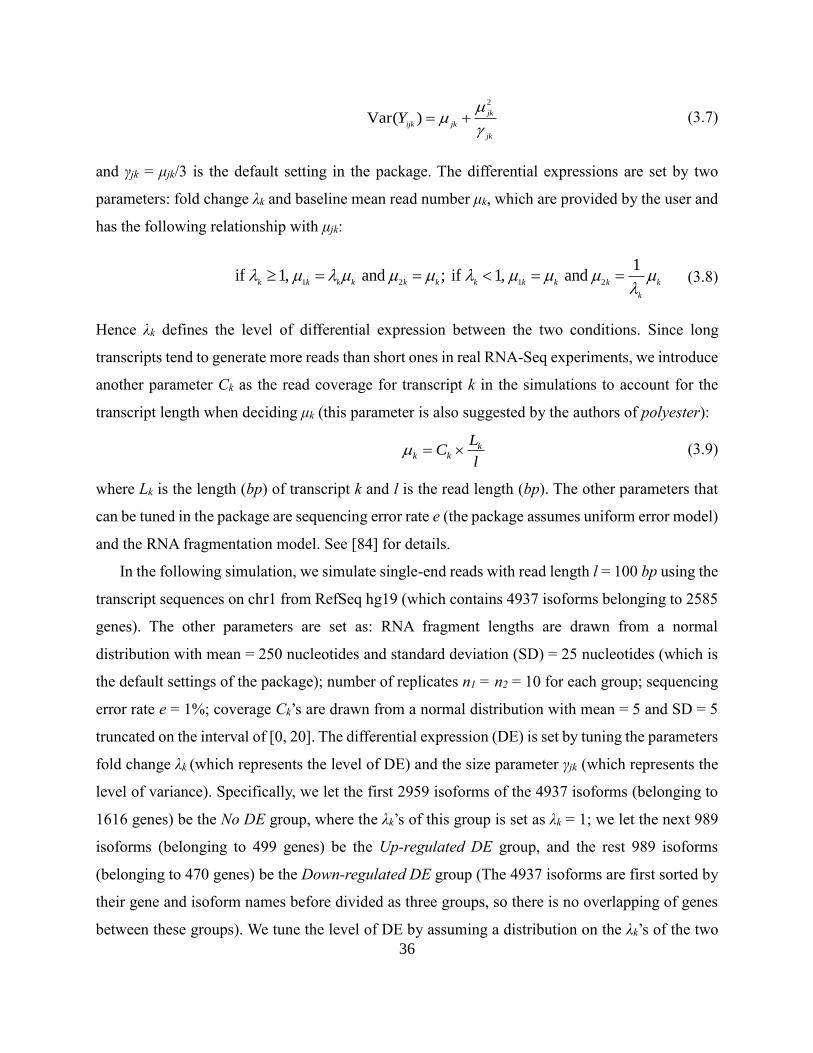
36
2
Var( )jk
ijk jk
jk
Y
(3.7)
and γjk = μjk/3 is the default setting in the package. The differential expressions are set by two
parameters: fold change λk and baseline mean read number μk, which are provided by the user and
has the following relationship with μjk:
1 12 2
1if 1, and ; if 1, and
k k k kk k k k k k
k
k
(3.8)
Hence λk defines the level of differential expression between the two conditions. Since long
transcripts tend to generate more reads than short ones in real RNA-Seq experiments, we introduce
another parameter Ck as the read coverage for transcript k in the simulations to account for the
transcript length when deciding μk (this parameter is also suggested by the authors of polyester):
kk k
LC
l (3.9)
where Lk is the length (bp) of transcript k and l is the read length (bp). The other parameters that
can be tuned in the package are sequencing error rate e (the package assumes uniform error model)
and the RNA fragmentation model. See [84] for details.
In the following simulation, we simulate single-end reads with read length l = 100 bp using the
transcript sequences on chr1 from RefSeq hg19 (which contains 4937 isoforms belonging to 2585
genes). The other parameters are set as: RNA fragment lengths are drawn from a normal
distribution with mean = 250 nucleotides and standard deviation (SD) = 25 nucleotides (which is
the default settings of the package); number of replicates n1 = n2 = 10 for each group; sequencing
error rate e = 1%; coverage Ck’s are drawn from a normal distribution with mean = 5 and SD = 5
truncated on the interval of [0, 20]. The differential expression (DE) is set by tuning the parameters
fold change λk (which represents the level of DE) and the size parameter γjk (which represents the
level of variance). Specifically, we let the first 2959 isoforms of the 4937 isoforms (belonging to
1616 genes) be the No DE group, where the λk’s of this group is set as λk = 1; we let the next 989
isoforms (belonging to 499 genes) be the Up-regulated DE group, and the rest 989 isoforms
(belonging to 470 genes) be the Down-regulated DE group (The 4937 isoforms are first sorted by
their gene and isoform names before divided as three groups, so there is no overlapping of genes
between these groups). We tune the level of DE by assuming a distribution on the λk’s of the two

37
DE groups. Let βk = log2 λk and the following four scenarios are simulated:
Scenario 1 - Low DE, Low variance: for Up-regulated DE group, βk’s are drawn from a normal
distribution with mean = 0 and SD = 0.5 truncated on the interval of [log21.25, +∞); for Down-
regulated DE group, βk’s are drawn from a normal distribution with mean = 0 and SD = 0.5
truncated on the interval of (-∞, -log21.25]; γjk = μjk/3 [which means the variance is 4μjk. See
equation (3.8)].
Scenario 2 - High DE, Low variance: for Up-regulated DE group, βk’s are drawn from a normal
distribution with mean = 0 and SD = 2 truncated on the interval of [log21.25, +∞); for Down-
regulated DE group, βk’s are drawn from a normal distribution with mean = 0 and SD = 2 truncated
on the interval of (-∞, -log21.25]; γjk = μjk/3.
Scenario 3 - Low DE, High variance: for Up-regulated DE group, βk’s are drawn from a normal
distribution with mean = 0 and SD = 0.5 truncated on the interval of [log21.25, +∞); for Down-
regulated DE group, βk’s are drawn from a normal distribution with mean = 0 and SD = 0.5
truncated on the interval of (-∞, -log21.25]; γjk = μjk/7 [which means the variance is 8μjk. See
equation (2.8)].
Scenario 4 - High DE, High variance: for Up-regulated DE group, βk’s are drawn from a normal
distribution with mean = 0 and SD = 2 truncated on the interval of [log21.25, +∞); for Down-
regulated DE group, βk’s are drawn from a normal distribution with mean = 0 and SD = 2 truncated
on the interval of (-∞, -log21.25]; γjk = μjk/7.
Note that in Scenarios 1 and 3, the SD of βk’s is small and fewer isoforms (genes) have high
fold changes, hence these two scenarios are termed “Low DE”; while in Scenarios 2 and 4, the SD
of βk’s is large and more isoforms (genes) have high fold changes, hence these two scenarios are
termed “High DE”.
For each scenario, the reads are simulated according to equations (3.6) - (3.9) using polyester
and mapped to the reference transcript sequences using Bowtie (version 1.1.1) under default
settings with number of mismatches of no more than two [85]. RSEM (version v1.2.14) is used for
quantification of the expression values of the isoforms and genes with default settings [77]. Then
we apply rSeqNP and EBSeq [40] to test for differential expression and splicing. For rSeqNP, FDR
≤ 0.05 is used as the cut-off of calling a gene or isoform showing DE (here we use FDR as the
criterion instead of p-value since we need to use the same metric for comparisons between rSeqNP

38
and EBSeq. See below); for EBSeq, posterior probability of being differentially expressed (PPDE)
≥ 0.95 is used as the cut-off of calling a gene or isoform showing DE. PPDE is the metric reported
by EBSeq and PPDE ≥ 0.95 corresponds to controlling FDR at 5% [40]. Specifically, we calculate
the false discovery proportion (FDP), type I error rate and power for each testing method as
Number of genes/isoforms from the No DE group detected as DE by the tests
Number of genes/isoforms detected by the tFDP
ests
Number of genes/isoforms from the No DE group detected as DE by the teststype I error rate
Number of genes/isoforms from the No DE group
Number of genes/isoforms from the DE group detected as DE by the testspower
Number of genes/isoforms from the DE group .
The results are shown in Table 3.5. We also draw the ROC curves and calculate the area under
the curve (AUC) statistics for each testing method based on the knowledge of the true differential
status of each gene (isoform), which are shown in Figure 3.1 and Table 3.5, respectively.
The results show the FDPs and type I error rates are controlled at 5% in general, though some
FDPs from rSeqNP are slightly higher than 5%. As expected, the sensitivity (power) and specificity
for each testing method decrease from high DE to low DE scenarios, and also decrease from low
variance to high variance scenarios. When the level of DE is low, the permutation test based on
the GDS has higher powers and AUCs than other testing methods. When the level of DE is high,
performances of EBSeq and rSeqNP are similar. EBSeq has slightly higher powers and AUCs
(Table 3.5 and Figure 3.1).

39
Figure 3.1 ROC curves of different testing methods in each scenario of the simulations.
(A) Low DE, Low variance (B) Low DE, High variance (C) High DE, Low variance (D) High DE,
High variance. EBSeq.Iso and EBSeq.Gene represent the tests for isoforms and genes in EBSeq
package, respectively. rSeqNP.WRS.Iso and rSeqNP.WRS.Gene represent the Wilcoxon rank-sum
tests for isoforms and genes in rSeqNP package, respectively. rSeqNP.GDS represents the
permutation test based on the GDS in rSeqNP package.

40
Table 3.5 FDP, type I error rate, power and AUC of different testing methods in each scenario
in the simulations
Low variance High variance
Test Methodsa FDP Type I Power AUC FDP Type I Power AUC
Low DE
EBSeq
Gene.D
E
0.5% 0.7% 81.0% 0.937 1.5% 0.8% 68.7% 0.919
Iso.DEb 2.0%
(1.4%)
1.0%
(0.5%)
77.5%
(55.4%)
0.906 4.3%
(3.2%)
1.8%
(1.0%)
62.6%
(43.7%)
0.866
rSeqNP
Gene.D
E
3.6% 2.8% 84.3% 0.946 4.2% 1.9% 69.1% 0.903
Iso.DEb 5.3%
(3.1%)
2.3%
(1.3%)
82.4%
(62.6%)
0.892 6.1%
(4.1%)
2.5%
(1.4%)
65.1%
(46.7%)
0.857
GDS 4.4% 1.9% 84.5% 0.964 5.9% 2.6% 70.9% 0.944
High DE
EBSeq
Gene.D
E
1.1% 0.6% 94.5% 0.992 0.9% 0.5% 87.7% 0.982
Iso.DEb 3.6%
(2.0%)
2.0%
(1.1%)
94.1%
(85.2%)
0.967 3.5%
(2.1%)
1.9%
(1.2%)
87.7%
(81.0%)
0.960
rSeqNP
Gene.D
E
6.5% 3.9% 93.9% 0.966 4.2% 2.3% 87.5% 0.954
Iso.DEb 6.4%
(3.9%)
3.8%
(2.3%)
93.4%
(85.8%)
0.949 5.6%
(3.4%)
3.1%
(1.9%)
87.1%
(80.7%)
0.940
GDS 6.7% 4.3% 93.9% 0.963 5.8% 3.2% 87.4% 0.949
a. For EBSeq, Gene.DE and Iso.DE represent the tests for genes and isoforms, respectively. For
rSeqNP, Gene.DE and Iso.DE represent the Wilcoxon rank-sum tests for genes and isoforms,
respectively, and GDS represents the permutation test based on GDS.
b. % of genes (% of isoforms).

41
3.4 Application to a prostate cancer RNA-Seq dataset
Here we apply rSeqNP to a real RNA-Seq dataset and compare it with EBSeq [40] and Cuffdiff
[37], which are two existing approaches for detecting differential expression of genes and isoforms
from RNA-Seq data. The dataset was generated from paired-end RNA-Seq experiments performed
on prostate cancer samples and matched benign samples from 14 Chinese prostate cancer patients
[86] and the raw sequence files in FSATQ format can be downloaded from the ArrayExpress
database of the European Bioinformatics Institute with the accession number E-MTAB-567.
We use the RefSeq annotated genes and isoforms for the analysis, which has 24900 genes and
45713 isoforms in total. For RSEM version 1.2.14 [77] - EBSeq version 1.5.3 [40] and Cuffdiff
version 2.1.1 [37], we follow their user manuals and use the default parameters (RSEM-EBSeq,
see: http://deweylab.biostat.wisc.edu/rsem/README.html; Cuffdiff, see:
http://cufflinks.cbcb.umd.edu/manual.html). For our rSeq - rSeqNP pipeline, the script that we
used is provided as a testing example in the user manual of rSeqNP (http://www-
personal.umich.edu/~jianghui/rseqnp/). We note that both EBSeq and Cuffdiff remove genes with
very low expression levels from the analysis, therefore we also filter out genes with average
expression levels less than 0.5 RPKM in rSeqNP, which yields 14791 genes and 23197 isoforms
in the analysis. Users can set different criteria to filter out lowly expressed genes when using
rSeqNP. Since neither EBSeq nor Cuffdiff can handle paired two-group comparison, we run all
three programs on the dataset under the setting of unpaired two-group comparison, i.e. treat cancer
and benign samples as two distinct groups, as well as run rSeqNP under the setting of paired two-
group comparison. For preprocessing, we use the programs suggested by each of the three
approaches to quantify expression values for all the genes and isoforms: RSEM [77] for EBSeq,
rSeq [9] for rSeqNP and the integrated quantification program for Cuffdiff. We compare the
quantification results of isoform expression from rSeq, RSEM and Cuffdiff, which is shown in
Figure B.2. The result shows that the three programs provide very consistent and similar results
for quantification.

42
Figure 3.2 Comparison of quantification results of isoform expression by rSeq, RSEM and
Cuffdiff.
(A) RSEM v.s. rSeq (B) Cuffdiff v.s. rSeq. The log2 transformed estimated isoform expression
levels in the benign tissue sample from Patient #1 are plotted. A small value (0.1) is added to the
isoform expression values before taking logarithm. r: Pearson’s correlation coefficient; ρ:
Spearman’s correlation coefficient.
The numbers of differentially expressed and spliced genes identified by each program is shown
in Table 3.6. We use FDR≤0.05 for rSeqNP and Cuffdiff, and posterior probability of being
differentially expressed (PPDE)≥0.95 for EBSeq to call a differential event. PPDE is the metric
reported by EBSeq and PPDE≥0.95 corresponds to controlling FDR at 5%. As expected, when
treating the data as two distinct groups, rSeqNP detects fewer differentially expressed genes and
isoforms, but by applying the GDS, more differentially expressed or spliced genes are detected.
Furthermore, when accounting for the paired two group nature of the data, rSeqNP detects even
more differential events. We find that Cuffdiff detects a much smaller number of differentially
expressed or spliced genes, which is consistent with report from another study [87].
We also compare the performance of the permutation test based on the GDS with Wilcoxon rank-
sum test and Wilcoxon signed-rank test, which is shown in Figure 3.3. When treating the data as
unpaired two-group comparison, Wilcoxon rank-sum test identifies 3707 genes as either
differentially expressed or differentially spliced (the union of the 3346 genes and 2792 genes in
Table 3.6), which has a large proportion of overlap with those differential genes (4122) identified
by the permutation test based on the GDS (Figure 3.3A). The result is similar for treating the data

43
as paired two-group comparison (5150 differential genes identified by Wilcoxon signed-rank test,
which is the union of the 4544 genes and 4163 genes in Table 3.6, and 6050 differential genes
identified by the permutation test based on the GDS. Figure 3.3B). But the permutation test based
on GDS can also identify many distinct differential genes that Wilcoxon rank-sum test and
Wilcoxon signed-rank test fail to detect, and two of such examples are given in Figure 3.4.
Figure 3.4 shows two individual genes to demonstrate the strength of the paired two-group
comparison over the unpaired two-group comparison (Figure 3.4A) and the strength of the
permutation test based on the GDS (Figure 3.4B). In Figure 3.4A, the ABDH8 gene has only one
isoform (NM_024527), which is down-regulated in the tumor samples of all the 14 patients. The
test results for this gene are: paired two-group Wilcoxon signed-rank test: p-value=1.22e-4,
FDR=4.50e-3; paired two-group permutation test based on the GDS: p-value=6.79e-5,
FDR=6.40e-4; unpaired two-group Wilcoxon rank-sum test: p-value=0.035, FDR=0.149; unpaired
two-group test by EBSeq: PPDE=0.917 (FDR=0.083). The test based on paired two-group
comparison can successfully capture this differential event.
In Figure 3.4B, the PKN1 gene is identified as differential by the paired two-group permutation
test based on the GDS (p-value=0.0392, FDR=0.0463) but not by the Wilcoxon signed-rank test
(results for the Wilcoxon signed-rank test are: test of DE for the gene: p-value=0.583, FDR=0.706;
test for Isoform NM_002741: p-value=0.676, FDR=0.180; test for Isoform NM_213560: p-
value=0.153, FDR=0.312). We can see that NM_002741 is down-regulated in tumor samples in 9
out of the 14 patients, while NM_213560 is up-regulated in tumor samples in 10 out of the 14
patients. Interestingly, the expression levels of the two isoforms show reverse directions in 9
patients (i.e. one is down-regulated in tumor samples while the other is up-regulated in tumor
samples). This gene might be of interest to follow up in the down-stream experiments by biologists.
The strength of the permutation test based on the GDS is that it can capture the differential genes
showing this type of patterns.

44
Table 3.6 Numbers of genes identified by different programs from the prostate cancer RNA-
Seq dataset
rSeqNP
(unpaired)
rSeqNP
(paired)
EBSeq
(unpaired)
Cuffdiff
(unpaired)
Gene.DE 3346 4544 2514 14
Isoform.DEa 2792
(2933) 4163
(4453)
3279
(4323)
26
(31)
GDS 4122 6050 - -
a. Number of genes (Number of isoforms) that are detected.
Figure 3.3 Comparison of the permutation test based on the GDS with Wilcoxon rank-sum
test (WRS) and Wilcoxon signed-rank test (WSR).
(A) Treating the data as unpaired two-group comparison: compare the genes identified by the
permutation test based on the GDS and by WRS. (B) Treating the data as paired two-group
comparison: compare the genes identified by the permutation test based on the GDS and by WSR.

45
Figure 3.4 Two individual gene examples to demonstrate the strength of the paired two-group
comparison and the permutation test based on the GDS.

46
(A) The ABHD8 gene showing the strength of the paired two-group comparison over the unpaired
two-group comparison. (B) The PKN1 gene showing the strength of the permutation test based on
the GDS over the Wilcoxon signed-rank test. In the bar plot, the difference of isoform expression
levels between tumor and matched normal tissue samples are plotted for each patient. The tables
below the plots show the estimated expression values (in RPKM unit) by rSeq for tumor (T) and
matched normal (N) tissue samples for each patient.
Finally, we check the robustness of our non-parametric approach. We run rSeqNP without
filtering out genes with low expression levels (i.e. using the expression values of all 24900 genes
and 45714 isoforms as input data) and compare the results with those after filtering the noisy genes
(see Table 3.6), which are shown in Table 3.7. We can see that the non-parametric approach is
generally robust to noisy genes, with only several hundreds of genes affected.
Table 3.7 Number of differential genes identified by rSeqNP without filtering noisy genes in
the prostate cancer RNA-Seq dataset.
unpaired overlapa paired overlapb
Gene.DE 3209 2863 4429 4018
Isoform.DEc 2409(2505) 2229(2317) 3516(3694) 3370(3124)
GDS 3480 3045 5555 5457
a. This compares the overlap with Column 1 in Table 3.6.
b. This compares the overlap with Column 2 in Table 3.6.
c. Number of genes (Number of isoforms) that are detected.
3.5 Conclusion
We present rSeqNP, a non-parametric approach for detecting differentially expressed and
spliced genes from RNA-Seq data. It is flexible in handling various types of experimental designs.
It is worth mentioning that, as pointed out by the reviewer, our method relies on expression
estimates for genes and isoforms reported from upstream programs, which are typically based on
parametric approaches. The major limitation of rSeqNP is that its power is relatively low for small
sample size RNA-Seq data. In simulation studies, we show that the power is decent with five or
more samples in each group for two-group comparison. If the sample size is even smaller,
parametric approaches would be preferred.

47
CHAPTER IV
A Two-part Mixed Model for Differential Expression Analysis in Single-cell High-
throughput Gene Expression Data
The gene expression data generated from more recent single-cell RNA-Seq and parallel single-
cell qRT-PCR technologies enable biologists to study the function of transcriptome at the level of
individual cells. Compared with regular RNA-Seq and qRT-PCR, single-cell gene expression data
show notable distinct features, including excessive zero expression values, high variability and
clustered design. In this chapter, we propose to model single-cell gene expression data using a two-
part mixed model. This model not only adequately accounts for the above features of single-cell
expression data, but also provides the flexibility of adjusting for covariates. An efficient
computational algorithm, automatic differentiation, is used for estimating the model parameters.
Compared with existing methods, our approach shows improved power for detecting differential
expressed genes in single-cell gene expression data.
4.1 Introduction
Recently, single-cell high-throughput gene expression profiling technologies, including single-
cell RNA-Seq (scRNA-Seq) and parallel single-cell qRT-PCR (scRT-PCR) have enabled
researchers to examine mRNA expression at the resolution of individual cells, which provide
further biological insights of the transcriptomes and functional genomics [43,88-90]. Compared to
regular RNA-Seq and qRT-PCR experiments that performed on tissues (i.e. cell populations) and
homogenous cell lines, single-cell gene expression data have the following distinct features as
demonstrated in recent literature [43,91,92]:
Excessive zero expression values. The proportions of genes with observed zero expression
values in single-cell gene expression data are much larger than regular RNA-Seq or qRT-PCR data
[43,91,92]. The reasons for this phenomena can be either biological, such that the abundance of

48
mRNA levels of certain transcripts are essentially low in individual cells, or can be technical, such
that the extracted total amount of mRNA is low in an single cell sample [43,92].
High variability of expression levels across samples. It has been observed that scRNA-Seq or
scRT-PCR data tend to show higher variability than bulk RNA-Seq or qRT-PCR data [43,92]. This
can be explained by the differences of the designs between the two: the regular bulk RNA-Seq or
qRT-PCR experiments are performed on the cell populations and the gene expression levels from
those experiments are averaged across all individual cells in the population, which dilutes the
variability of gene expression levels among individual cells [92].
Clustering of single-cell samples within subjects. Another notable feature of single-cell high-
throughput gene expression data is that each individual single-cell samples are randomly sampled
from a higher-level of cluster unit (e.g. patients, animals) [44,88,89]. Therefore, the single-cell
samples from the same subject are expected to be more homogeneous than those from different
subjects, which has been shown in several single-cell RNA-Seq data published recently [44,88,89].
From a statistical point of view, this feature is called cluster effect, which should be adequately
adjusted for in the analysis.
Based on the above discussions, we propose to model single-cell gene expression data using a
two-part mixed model. This model not only adequately accounts for the above features of single-
cell expression data, but also provides the flexibility of adjusting for covariates. The rest of this
chapter is organized as follows: First we describe the formulation of the two-part mixed model
with a brief literature review. Then we use an efficient method, named automatic differentiation,
to fit the model. We also discuss how to test for differential expression under this model and
describe several methods for approximating the null distribution of the test statistics for small
sample sizes, followed by simulations for studying the type I error rate and statistical power.
Finally, we demonstrate our approach by applying it to two real datasets: one from scRT-PCR and
one from scRNA-Seq.
4.2 Methods
4.2.1 The two-part mixed model for single-cell gene expression data
We first introduce the notations in this section. Assume there are m subjects and N genes in a
scRNA-Seq experiment, and ni single cell samples extracted and sequenced for subject i (i = 1,…,

49
m). Let yijk be the normalized expression value (in the unit of RPKM/FPKM, TPM or CPM) for
gene k (k = 1,…, N) in single-cell sample j (j = 1,…, ni) in subject i, then we model the gene
expression value yijk using the following two-part mixed model:
logit[Pr( 0)] log( ) ,1
log( | 0) ,
ijk T
ijk jk k ik
ijk
T
ijk ijk jk k ik ijk
y u
y c y v e
w α
x β
(4.1)
where πijk is the proportion of single cell samples with zero expression values for gene k (named
as “zero-proportion” hereafter). In this two-part model, the zero-proportions are modelled by a
logistic regression model (logistic or binomial part), and the log transformed non-zero
expression values are modeled by a linear regression model (Gaussian part), where T
jkw and T
jkx
are the vectors of covariates for the binomial and Gaussian parts respectively (for example, if
there are only two biological conditions and no other covariates to be adjusted, T
jkw and T
jkx are
simply the vectors of 1/0 indicators for the biological conditions), k
α and kβ are the
corresponding vectors of regression coefficients for the covariates T
jkw and T
jkx , eijk is the
random error that is assumed to be distributed as 2(0, )eN , uik and vik are the random effects
for subject i that account for the cluster effect which are assumed to follow the bivariate normal
distribution
2
2~ ( , )
ik u u v
ik u v v
uN
v
0
with 2
u and 2
v as the variances for the marginal univariate normal distributions of uik and vik,
and ρ as the correlation between them. We note that most scRNA-Seq experiments contain only
one-level of clusters (i.e. single cells are sampled from subjects). If the study design is more
complicated such that it may contain multi-level cluster effects, then more variance components
for the random effects can be added in the model. Finally, a small constant c is added to the non-
zero expression levels before taking logarithms to avoid the left skewness caused by taking
logarithms on small expression values between 0 and 1, which is often seen in RNA-Seq data.
In the following analysis of scRNA-Seq data, c is set as 1.
In scRT-PCR experiment, the gene expression levels are usually measured by the expression
threshold (et) values, which is defined as max
et c ct , where cmax is the maximum number of

50
amplification cycles used in the scRT-PCR experiment and ct is the threshold cycle that the gene
is detected by the PCR instrument [91]. The gene expression level yijk is assumed to have an
exponential relationship with et, such that 2e
ijk
ty (for undetected genes, et is shown as
missing values from the PCR machine and can be treated as -∞, which gives zero expression
values) [91]. Therefore (4.1) can also be used to model gene expression values in scRT-PCR
data, and the definitions of the parameters are exactly the same as those in scRNA-Seq data.
The only difference is that adding the small constant c is not necessary for scRT-PCR, as the
non-zero gene expression levels in scRT-PCR experiments do not have many small values
between 0 and 1 like those in scRNA-Seq data.
Remark on related literature: The two-part model including the binomial part and Gaussian
part without random effects is first proposed by Duan et al for modeling the medical care data
[93,94], where the dependent variable (medical care expenses) takes the range of any
nonnegative value, but has a positive probability at zero (this type of data are also called
semicontinuous data) [93-95]. Olsen et al extend the two-part model for longitudinal or
clustered semicontinuous data by incorporating random effects for both the binomial part and
the Gaussian part [96]. A comprehensive survey for a variety of models with applications for
data taking non-negative values with a substantial proportion of zero values is given in [95].
Our two-part mixed model (named TMM hereafter) essentially follows the model formulation
in [95,96], except the addition of a small constant c to the non-zero expression values in RNA-
Seq data [model (4.1)]. A similar, yet different two-part model without random effects is
proposed to model the single-cell RNA-Seq data in a recent paper (named MAST hereafter) [45].
Instead of incorporating clustered random effects from subjects, MAST uses an empirical Bayes
method to shrink the gene-specific variance to the global variance of all genes [45].
4.2.2 Model fitting for TMM
Since the TMM model (4.1) is fitted for each gene independently, we will drop the subscript
k for simplicity if there is no ambiguity within the context. Following [96], the fixed-effect
parameters of the TMM model, k
α and kβ are estimated by maximizing the following marginal
likelihood function of the model

51
1( , )
i i
m
B G i i i iiL L L p u v du dv
(4.2)
where iBL is the conditional distribution (likelihood) of yijk given the random effect ui from the
binomial (logistic) part
1, 0 1
1[ exp( )][ ]
1 exp( )
i i
i
ij
n nT
B j j i Tj y j j j i
L uu
w αw α
,
iGL is the conditional distribution (likelihood) of yijk given the random effect vi from the
Gaussian part
1
1, 0
log( 1)[ ]
i
i
ij
Tnij j j i
G e
j y e
y vL
x β
with ϕ(•) as the standard normal PDF [for scRT-PCR data, log(yij+1) becomes log(yij)], and
( , )i ip u v is the joint distribution of the random effects ui and vi. Throughout this chapter, we
only fit the model with independent random effects ui and vi for computation efficiency, but
note that the model with correlated random effects as discussed in Section 4.2.1 can also be
fitted. Under the assumption that ui and vi are independently distributed as 2(0, )u
N and
2(0, )v
N , their joint distribution can be written as the product of two univariate normal
distributions
1 1( , ) [ ( )][ ( )]i ii i u v
u v
u vp u v
As discussed in [96] and [95], maximizing the marginal likelihood function (4.2) involves
numerical or stochastic approximation of the integrals, followed by maximization of the
approximated likelihood. Several computational methods, including the Markov chain Monte
Carlo, the expectation-maximization (EM) algorithm, the penalized quasi-likelihood (PQL)
method, Gauss-Hermite quadrature and Laplace approximations are reviewed and discussed in
details in [96]. Here, we use an efficient computational method, called automatic differentiation,
to maximize the likelihood function (4.2). The automatic differentiation technique is
implemented in the software package automatic differentiation model builder (ADMB, version
11.4) [97,98]. Given the likelihood function written in the form of (4.2), ADMB calculates the
Hessian matrix of the marginal likelihood function using the automatic differentiation technique,
and the maximization of the marginal likelihood function is performed by first approximating

52
the integrals using Laplace approximations and then maximizing the approximated likelihood
using the quasi-Newton algorithm. Descriptions of the automatic differentiation technique can
be found in [97,98] and the details for implementation of the algorithm can be found in the
manuals of ADMB, which are available at http://www.admb-project.org/docs/manuals.
4.2.3 Testing for differential expression
Testing for differential expression of genes across biological conditions under model (4.1)
is done by testing for the fixed effects. More explicitly, (4.1) can be written as
1 1 2 2
1 1 2 2
logit[Pr( 0)] log( ) ,1
log( 1 | 0) ,
ij T T
ij j j i
ij
T T
ij ij j j i ij
y u
y y v e
w α w α
x β x β
(4.3)
where 1
T
jw and
1
T
jx are the covariates of interest that we want to test for, and
2
T
jw and
2
T
jx are the
covariates to be adjusted for in the model. Specifically, we are interested in testing for the
following two effects across biological conditions: 1). Whether the zero-proportions are
significantly different across conditions and 2). For genes with non-zero expression levels,
whether the mean expression levels are significantly different across conditions. The two
problems can be formulated as the following two corresponding hypothesis testing problems:
1) Testing of the binomial part
0 1 1 1: 0 versus : 0
B BH H α α
2) Testing of the Gaussian part
0 1 1 1: 0 versus : 0
G GH H β β
and the two parts can also be tested jointly, which can improve the statistical power:
3) Joint testing of the binomial and Gaussian parts
0 1 1 1 1 1: 0 and 0 versus : 0 or 0H H α β α β
The individual test for the binomial part or the Gaussian part can be performed using the Wald
test or the likelihood ratio test, and the joint test for the two parts can be performed using the
likelihood ratio test. Under H0, the asymptotic distributions of the Wald statistic (W0) and the
likelihood ratio statistic (L0) can be approximated by the χ2 distribution with the degrees of
freedom equal to the differences in the numbers of parameters between H0 and H1, which is a
widely used approach in practice [99,100]. However, for small sample sizes, the χ2 distributions

53
are not good approximations to the null distributions of the two test statistics, which, as noted
in the literature [99,101] and as shown in simulations in Section 4.3, often show inflated type I
error rate. Therefore, we use the following two methods for reliable estimation of p-values when
the sample size is small:
The parametric bootstrap method: this approach estimates the null distribution of the test
statistic by simulating data from the fitted model under H0, which is performed in the following
way [101-104]:
(1) Fit model (4.3) under H0 and generate N random samples 1,...,
Ny y from
0
ˆHf .
(2) Calculate the corresponding test statistics (i.e., Wald or likelihood ratio statistics)
1,( ) ), (
NT Ty y using the simulated samples
1,...,
Ny y .
(3) Estimate the p-value as 1
1ˆ { ( ) }
N
l
l
p I TN
y (an alternative formula is
1
{ ( ) } 1
ˆ1
N
l
l
I T
pN
y
. The two formulas give almost the same results providing N is large, so
we use the former throughout this chapter).
The empirical Satterthwaite method: this method is proposed by Cai et al [105], and it is a
general approach for approximating the null distribution of the test statistics [101,105-107].
Following [105,106], this method is performed in the following two steps:
(1) Approximate the null distribution of test statistics (W0 or L0) by a scaled χ2 distribution 2
vk
with k as the scale parameter and v as the degrees of freedom. The parameters k and v can be
estimated by matching the first two moments (sample mean and variance) of test statistics under
H0 with those of 2
vk [105,106]. The sample mean and variance of test statistics under H0 can
be obtained using permutations or the above parametric bootstrap method with a smaller number
of random samples.
(2) Fit a two component normal mixture distribution 2 2
1 1 1 2 2 2( , ) ( , )N N on 2
1 ( )( )v
b
kp
,
where 2
( )
v
b
kp
is the p-value obtained from the above scaled χ2 distribution 2
vk for the bth
permutated or bootstrapped random sample and Φ(•) is the standard normal CDF. The final p-
values are calculated as

54
2
1Pr[ ( )]vk
p p
where 2vk
p
is the p-value obtained from Step (1) and Ψ is the fitted normal mixture distribution
2 2
1 1 1 2 2 2ˆ ˆ ˆ ˆ ˆ ˆ( , ) ( , )N N .
The Satterthwaite method can estimate p-values using a smaller number of random samples
than the parametric bootstrap method [105,106]. However, in our simulations it also shows
inflated type I error rate when the sample size is small (see simulations in the next section).
4.3 Simulation studies
4.3.1 Evaluation of type I error rates
In this section, we evaluate type I error rates of the three methods for approximating the null
distribution of the test statistics under H0: the χ2 distribution, the Satterthwaite method and the
parametric bootstrap method. The simulations are performed based on the following settings:
Assuming two biological conditions, each has m/2 subjects, and for each subject i there are ni
single cell samples. To evaluate type I error rates, we simulate gene expression levels yijk from the
following model under H0 (i.e. there is no difference between the two conditions):
1
1
logit[Pr( 0)] log( ) ,1
log( 1 | 0) ,
ijk
ijk i
ijk
ijk ijk i ij
y u
y y v e
with 2~ (0, )i u
u N , 2~ (0, )i v
v N and 2~ (0, )ij e
e N
In this model, there is only one intercept for the fixed effect in both the binomial and Gaussian
parts, therefore no differences in terms of zero-proportions and mean expression levels are
expected between the two conditions. The values of the parameters are set as follows: 0.5u
,
1v
, 0.5e
, 2
1~ (0.5,0.25 )N , 2
1~ (3,0.5 )N , ni = 20 for all i’s (i = 1,…, m). We tune the
sample sizes by varying m for three different values 4, 10 and 20 respectively, which correspond
to small, moderate and large sample sizes. The simulations are repeated 1,000 times for different
m’s. For each run, we calculate the following five test statistics: Wald statistic for the Gaussian
part; Wald statistic for the binomial part; Likelihood ratio statistic for the Gaussian part; Likelihood

55
ratio statistic for the binomial part; Likelihood ratio statistic for jointly testing the Gaussian and
binomial parts. Then we calculate the p-values from each test using the three methods as described
in section 4.2.3.
If the type I error rate is correctly controlled, the p-values from the 1000 repetitions for each m
should be uniformly distributed within 0 to 1, so we examine each method using the quantile-
quantile plots of the p-values from the simulations (observed p-values) and the quantiles of
uniform [0, 1] distribution (expected p-values), which are shown in Figures 4.1 to 4.5. As seen in
these plots, all the three methods give well-controlled type I error rates for large samples sizes (m
= 20). However, for small sample sizes (m = 10 or m = 4) the performance of controlling type I
error rate of the three methods are ranked as (from the best to the worst): parametric bootstrap,
Satterthwaite, the χ2 distribution. And the inflation of type I error rate is more severe for the χ2
distribution with the test for the binomial part (Figure 4.2 and 4.4) or the joint test for the two parts
(Figure 4.5). On the other hand, the parametric bootstrap takes the longest computational time,
which can be overwhelming if we want to accurately estimate small p-values. As a general rule, if
the sample size is large, then the χ2 distribution can be used. If the sample size is small, then the
parametric bootstrap method should be preferred, with the cost of longer computational time. The
Satterthwaite method can be considered as an alternative method for moderate sample size.

56
Figure 4.1 Plots of the observed versus the expected p-values for the Wald test for the
Gaussian part under H0: no significant difference between the two conditions.
The p-values are plotted on -log10 scale. The gray areas represent the 95% confidence interval
bands of the expected p-values under H0.

57
Figure 4.2 Plots of the observed versus the expected p-values for the Wald test for the
binomial part under H0: no significant difference between the two conditions.
The p-values are plotted on -log10 scale. The gray areas represent the 95% confidence interval
bands of the expected p-values under H0.

58
Figure 4.3 Plots of the observed versus the expected p-values for the likelihood ratio test for
the Gaussian part under H0: no significant difference between the two conditions.
The p-values are plotted on -log10 scale. The gray areas represent the 95% confidence interval
bands of the expected p-values under H0.
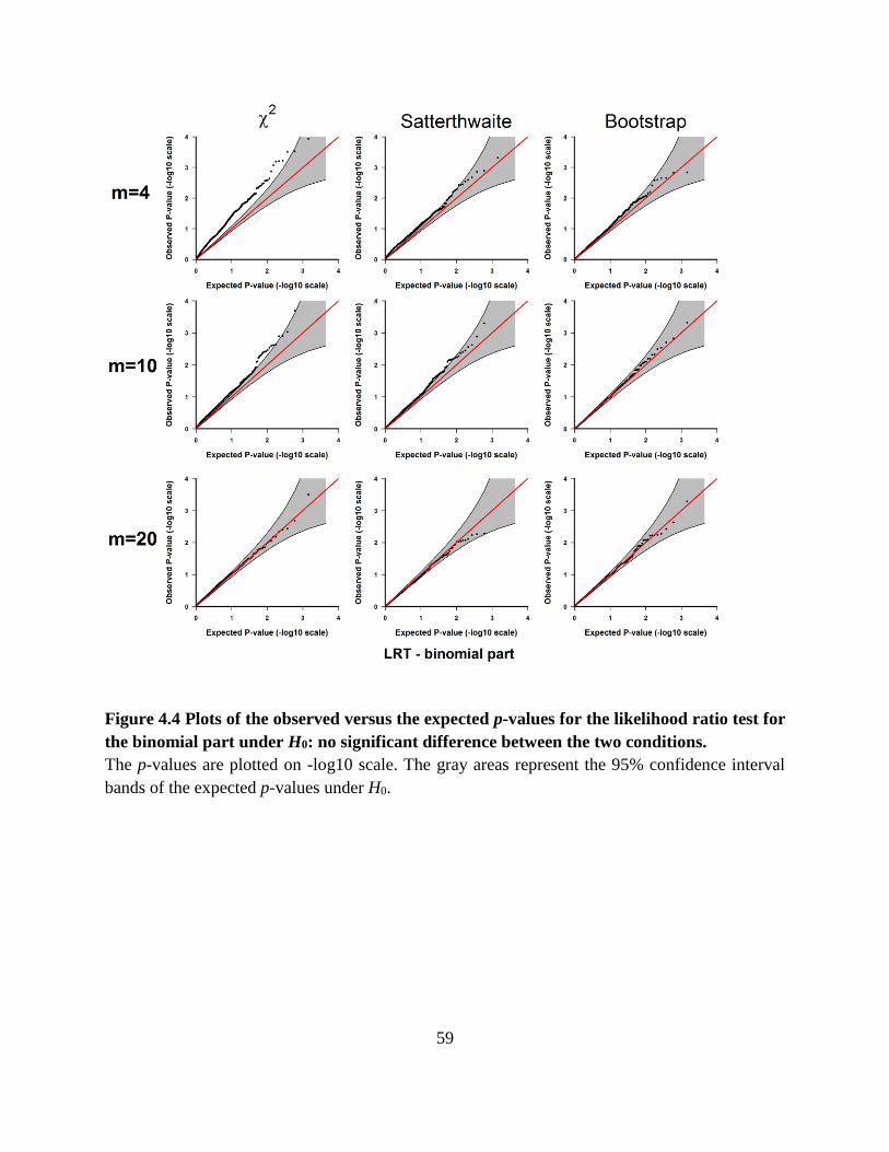
59
Figure 4.4 Plots of the observed versus the expected p-values for the likelihood ratio test for
the binomial part under H0: no significant difference between the two conditions.
The p-values are plotted on -log10 scale. The gray areas represent the 95% confidence interval
bands of the expected p-values under H0.

60
Figure 4.5 Plots of the observed versus the expected p-values for jointly testing the Gaussian
and binomial parts under H0: no significant difference between the two conditions.
The p-values are plotted on -log10 scale. The gray areas represent the 95% confidence interval
bands of the expected p-values under H0.
4.3.2 Evaluation of statistical power
In this section, we evaluate the statistical power of the TMM model, and compare it with a
published method MAST [45], and the two-part model with binomial and Gaussian parts but
without random effects (named TM hereafter). The simulations are performed based on the
following settings: suppose there are two biological conditions, and each condition has m/2

61
subjects, and for each subject i there are ni single cell samples sequenced. To evaluate the power,
we simulate the gene expression levels yijk from the following model under H1:
1 2
1 2
logit[Pr( 0)] log( ) ,1
log( 1 | 0) ,
ijk
ijk i
ijk
ijk ijk i ij
y w u
y y x v e
with 2~ (0, )i u
u N , 2~ (0, )i v
v N and 2~ (0, )ijk e
e N . In this model, w and x are 0/1 indicators of
the conditions, and the effect sizes are represented by the parameters 2
and 2
, which correspond
to the log odds of zero proportions and log fold change of the mean expression values for non-zero
genes between the two conditions. The values of the parameters are set as follows: m = 10, ni = 20
for all i’s (i = 1,…, m), 0.5u
, 1v
, 0.5e
, 2
1~ (0.25,0.25 )N , 2
1~ (3,0.5 )N . We then
tune the effect sizes by varying (2
,2
) for the following values: (0, 0), (0.25, 0.25), (0.5, 0.5),…,
(1.5, 1.5). The simulations are repeated 1000 times for each different pairs of (2
,2
)’s. In each
run, we apply our model TMM with the three methods for calculating p-values (the χ2 distribution,
the Satterthwaite and parametric bootstrap), MAST and TM respectively. The estimated power for
each method is calculated as the proportion of p-values less than 0.05 among the 1000 repetitions.
Figure 4.6 is the plots of power curves for each model with different effect sizes. As expected,
the power of each method increases with effect size. The power of TMM is consistently higher
than the other two models, which is also expected, since we include random effects in this
simulation setting.

62
Figure 4.6 Comparisons of statistical powers of different methods.
(A) Tests for the Gaussian part. (B) Tests for the binomial part. (C) Joint tests for the Gaussian and binomial parts. TMM: two-part
mixed model. “Chi-square”, “Satterthwaite” and “bootstrap”: the χ2 distribution, the Satterthwaite method and parametric bootstrap
method as described in Section 4.2.3. TM: the two-part model without random effects. The horizontal red dashed line represents the
level of the test, which is α = 0.05.

63
4.4 Application to real single cell gene expression data
In this section, we demonstrate our approach with application to two real single cell gene
expression datasets: one scRT-PCR dataset and one scRNA-Seq dataset.
4.4.1 Application to a scRT-PCR dataset
Here we apply the TMM model to a scRT-PCR dataset and compare the results with MAST.
This dataset is described in [108] and is incorporated with the MAST package [45], where 456
single cell samples of T cells from two patients with human immunodeficiency virus (HIV) are
isolated and the expression levels of 75 genes related to the immune system function are measure
by scRT-PCR. The activation of two immune-response proteins, T-cell receptor Vβ (TCR-Vβ) and
CD154, are used to categorized those T cells, and the 456 single cells are divided by the following
four different groups: TCR-Vβ+/CD154+, TCR-Vβ+/CD154-, TCR-Vβ-/CD154+ and TCR-Vβ-
/CD154-, where the TCR-Vβ+/CD154+ group is the activated T cells with normal immune
functions [108]. The goal of the analysis is to identify differentially expressed genes across the
above four groups.
We fit MAST and our TMM model to this dataset. Specifically, the covariates included in MAST
are
X1: a categorical variable indicating which of the above four groups the sample belongs to, where
the TCR-Vβ+/CD154+ is coded as the reference group. This variable is the one of our interest.
X2: a categorical variable indicating which of the two subjects that the sample is from.
For our TMM model, X1 is included as fixed effect in both the binomial part and the Gaussian part.
The two subjects are treated as two clusters, which are included as random effects in TMM. Since
the number of single cell samples is large in this scRT-PCR study, the χ2 distribution is used to
calculate p-values, and the likelihood ratio test is used to test the individual Gaussian part and
binomial part and also to jointly test the two parts.
The results from MAST and TMM for the 75 genes are shown in Table 4.1, and Figure 4.7 is a
graphical comparison of the p-values from the two methods. We can see that the results from the

64
two methods agree with each other in general, though some genes show different p-values from
the tests for the zero-proportions (binomial part) (Figure 7). This is expected as there are only two
clusters in this dataset, and the clustered random effects do not play a significant role in this
example. In fact, there should be a reasonable number of mixed levels to be included in a mixed
effect model to make it useful in practice [99]. Therefore, MAST should be preferred for this
dataset than TMM, and the application of TMM here is for the purpose of demonstration. On the
other hand, these results show that TMM is not essentially worse than MAST even the clustered
random effects are not significant.

65
Figure 4.7 Comparisons of the p-values from TMM and MAST for the scRT-PCR dataset.

66
The -log 10 of the p-values from both method are plotted. (B), (D) and (F) are respectively the zoom-in
parts of (A), (C) and (E) on the range of 0 to 10.

67
4.4.2 Application to a scRNA-Seq dataset
In this section, we apply the TMM model to a scRNA-Seq dataset and compare it with MAST
and TM. This dataset is published in [44], which contains 466 single cell samples from the human
brain tissues of 8 adults (aged from 21 to 63 years) and 4 fetuses (all aged 16 to 18 weeks), and
the expression levels of 22,088 genes in these samples are measured by scRNA-Seq [44]. The
dataset is available in NCBI Gene Expression Omnibus under accession number GSE67835.
The goal of our analysis is to identify differentially expressed genes between the adult and fetal
brains. We fit TMM with the following two covariates as fixed effects:
X1: a 0/1 indicator of biological conditions (adult versus fetus), which is the variable of interest.
X2: the gender of the subjects: male and female for adults. The gender of fetus is coded as a third
category, “undeveloped”.
and the twelve subjects are treated as clusters, which are included as random effects in the model.
Since the number of single cell samples is also large in this study, the p-values are estimated in the
same way as in the scRT-PCR dataset above. We also fit the MAST and TM models, where X1
and X2 are included as covariates in these two models. Multiple comparison adjustment is
performed using the Benjamini–Hochberg FDR procedure [109].
Figure 4.8 shows the number of differentially expressed genes identified by each method with
FDR<0.01, and Table 4.2 shows the p-values and FDR for the top 20 differentially expressed genes
(ranked by the p-values from the joint test for both the Gaussian and binomial parts under the
TMM model). We can see the results from the three models show considerable overlaps (Figure
4.8), and the top differentially expressed genes all show very significant p-values and FDR from
all methods. Notably, the total number of differentially expressed genes detected by TMM with
FDR<0.01 is much larger than the other two methods.

68
Figure 4.8 Number of differentially expressed genes identified by each method with
FDR<0.01.
(A) Gaussian part. (B) Binomial part. (C) Joint test for the Gaussian and binomial parts.
4.5 Discussion
In summary, we present a two-part mixed model (TMM) for differential expression analysis with
single cell gene expression data. This model not only adequately accounts for the distinct features
of single cell expression data, including extra zero expression values, high variability and clustered
design, but also provides the flexibility of adjusting for covariates. Since scRNA-Seq is still a
developing and growing technology, it brings more challenges in data analysis than regular RNA-
Seq. These challenges can be technical (for e.g., the number of samples in scRNA-Seq is large and
the sequencing experiments are performed in different batches [46], and also can be biological (for
e.g., the distinct features of the single cell expression data, as discussed in Section 4.1). Several
more recent studies show that several confounding factors often present in scRNA-Seq
experiments that can lead to biased results. These factors can also be categorized as technical
factors that are related to the design of experiments such as batch effects [46], or biological factors
such as the detection rate of genes [45,46], gene lengths and GC percent[46]. These confounding
factor can be adjusted in TMM, however planning a good study design for scRNA-Seq
experiments to reduce the confounding factors is a more fundamental task [46].

69
Table 4.1 Results of the gene differential expression analysis for the HIV scRT-PCR dataset.
Gene Name MAST TMM
Gaussian Binomial Combine Gaussian Binomial Combine
CD40LG 2.33E-46 9.87E-18 2.82E-61 3.73E-48 3.53E-17 1.72E-62
GAPDH 6.60E-27 8.44E-10 4.04E-34 1.78E-27 2.30E-10 2.82E-35
TNF 1.60E-03 7.70E-22 1.13E-22 3.48E-03 1.89E-22 7.94E-23
TGFB1 6.08E-18 2.73E-04 9.61E-20 1.75E-16 4.31E-04 5.01E-18
IL2 1.46E-03 4.53E-18 3.06E-19 2.39E-03 3.90E-18 2.05E-19
IL16 2.21E-01 9.21E-18 2.93E-16 4.90E-02 4.74E-18 2.42E-17
IL2Rg 6.80E-08 1.97E-10 3.72E-16 3.11E-09 2.08E-11 2.06E-18
CXCR4 7.89E-04 3.94E-14 1.33E-15 5.20E-04 1.71E-14 3.51E-16
CCR7 3.60E-01 8.61E-17 4.88E-15 4.20E-01 8.38E-17 3.54E-15
CD3d 3.69E-06 1.67E-10 1.65E-14 7.22E-07 2.33E-10 3.61E-15
IL2Ra 9.09E-03 5.14E-13 2.08E-13 1.18E-03 1.09E-12 6.11E-14
CD69 7.99E-06 2.06E-09 4.00E-13 3.34E-06 1.89E-09 1.80E-13
IL10 1.75E-01 3.88E-14 5.74E-13 3.25E-02 5.85E-14 1.44E-13
FASLG 6.47E-02 1.60E-12 3.73E-12 3.06E-02 1.33E-12 3.32E-12
IL7R 1.23E-06 2.18E-06 5.23E-11 9.05E-08 1.68E-06 4.57E-12
IL6ST 1.13E-03 4.49E-09 1.21E-10 1.14E-04 4.45E-08 1.12E-10
SLAMF1 3.45E-02 4.78E-10 5.56E-10 1.05E-02 2.95E-10 9.47E-11
IFNg 2.66E-05 1.47E-06 7.06E-10 2.39E-05 1.85E-06 5.83E-10
CD109 8.97E-01 8.36E-10 8.06E-09 7.76E-01 7.10E-10 7.65E-09
TNFRSF9 3.20E-01 2.38E-09 1.44E-08 2.13E-01 1.45E-09 8.35E-09
DPP4 2.96E-01 1.35E-09 1.91E-08 4.66E-02 2.03E-08 2.38E-08
ICOS 2.41E-05 6.80E-05 2.53E-08 8.93E-05 5.14E-04 4.77E-07
CD28 2.14E-01 3.34E-07 1.88E-06 3.67E-01 1.17E-06 9.26E-06
CD4 1.06E-01 1.47E-05 2.46E-05 1.04E-01 3.88E-05 6.66E-05
CD27 1.94E-01 2.86E-05 8.73E-05 1.01E-01 5.68E-06 1.20E-05
CD48 4.55E-01 1.69E-05 1.59E-04 3.52E-01 1.46E-06 2.14E-05
SLAMF5 5.39E-02 3.28E-04 1.89E-04 3.34E-02 4.43E-04 1.14E-04

70
CTSD 3.11E-03 7.58E-03 2.14E-04 3.59E-04 8.01E-03 2.68E-05
CD5 5.47E-01 3.30E-05 3.65E-04 3.80E-01 7.13E-06 4.89E-05
TBX21 1.71E-01 1.97E-04 4.06E-04 1.17E-01 8.15E-05 1.10E-04
CSF2 6.55E-01 2.46E-04 5.40E-04 1.00E+00 2.09E-04 5.13E-04
CD3g 9.95E-01 1.17E-05 6.03E-04 8.13E-01 7.87E-07 3.11E-05
TIA1 1.70E-02 1.29E-02 1.64E-03 9.89E-03 4.89E-03 3.84E-04
CD45 2.94E-01 8.41E-04 2.56E-03 1.72E-01 2.48E-03 3.63E-03
PECAM1 3.68E-02 1.21E-02 3.14E-03 7.98E-03 9.12E-03 5.55E-04
NT5E 5.96E-01 2.21E-03 6.24E-03 3.77E-01 1.28E-03 3.82E-03
LIF 7.70E-01 3.60E-03 1.17E-02 6.83E-01 1.00E+00 7.22E-01
FOXP3 8.77E-03 2.03E-01 1.21E-02 3.65E-03 2.02E-01 6.33E-03
TIMP1 2.18E-02 1.26E-01 1.62E-02 4.23E-02 7.55E-02 2.13E-02
CTLA4 3.26E-01 8.50E-03 1.92E-02 4.15E-02 1.70E-02 5.31E-03
FAS 7.88E-01 4.45E-03 3.49E-02 4.21E-01 4.76E-03 1.21E-02
RORC 8.99E-01 1.13E-02 3.61E-02 9.52E-01 7.71E-03 2.06E-02
CCR2 3.11E-02 2.07E-01 3.73E-02 1.42E-04 5.63E-01 9.61E-04
BCL2 2.34E-01 3.77E-02 4.15E-02 1.56E-01 1.00E+00 1.51E-01
PRDM1 1.36E-02 5.71E-01 5.18E-02 2.11E-03 7.40E-01 1.85E-02
CCL3 1.48E-01 1.01E-01 6.68E-02 4.16E-01 1.00E+00 3.36E-01
CCL2 8.07E-02 1.00E+00 8.07E-02 2.14E-01 1.00E+00 3.05E-01
IL8 1.03E-01 2.06E-01 9.36E-02 4.31E-01 1.07E-01 1.67E-01
CCL5 8.38E-02 2.80E-01 9.98E-02 3.18E-01 3.17E-01 2.20E-01
TNFSF10 3.27E-01 1.49E-01 1.76E-01 3.88E-01 2.06E-02 5.12E-02
CSF1 1.79E-01 4.38E-01 2.57E-01 1.23E-01 2.20E-01 9.77E-02
CCR4 4.57E-01 1.79E-01 2.66E-01 4.10E-01 1.59E-01 1.48E-01
HLADRA 1.61E-01 5.11E-01 2.73E-01 4.78E-01 1.21E-01 2.16E-01
BAX 9.26E-01 5.98E-02 2.86E-01 9.97E-01 2.79E-02 1.94E-01
CD38 4.60E-01 3.35E-01 4.09E-01 7.37E-01 2.11E-01 4.97E-01
SLAMF7 5.01E-01 1.00E+00 5.01E-01 1.00E+00 1.00E+00 1.00E+00
GATA3 1.36E-01 9.75E-01 5.11E-01 1.29E-01 8.29E-01 4.44E-01
PCNA 8.92E-01 3.40E-01 5.52E-01 8.19E-01 1.00E+00 1.00E+00

71
MMP9 6.35E-01 1.00E+00 6.35E-01 1.00E+00 1.00E+00 1.00E+00
ENTPD1 6.50E-01 1.00E+00 6.50E-01 2.97E-02 1.00E+00 3.10E-02
CCL4 6.79E-01 6.22E-01 7.55E-01 1.00E+00 1.00E+00 1.00E+00
PRF1 9.51E-01 4.12E-01 7.67E-01 7.96E-01 1.00E+00 1.00E+00
EOMES 7.68E-01 5.98E-01 7.89E-01 5.52E-01 1.00E+00 7.63E-01
IL6R 6.31E-01 7.39E-01 7.98E-01 2.22E-01 5.60E-01 5.96E-01
CCR5 4.52E-01 9.28E-01 8.09E-01 1.33E-01 5.54E-01 3.07E-01
GZMA 4.02E-01 9.95E-01 8.52E-01 2.78E-01 8.78E-01 7.79E-01
CD8a 9.58E-01 1.00E+00 9.58E-01 6.68E-01 1.00E+00 9.00E-01
B3GAT1 1.00E+00 1.00E+00 1.00E+00 1.00E+00 1.00E+00 1.00E+00
CXCL13 1.00E+00 1.00E+00 1.00E+00 1.00E+00 1.00E+00 1.00E+00
IL12RbII 1.00E+00 1.00E+00 1.00E+00 1.00E+00 1.00E+00 1.00E+00
IL13 1.00E+00 1.00E+00 1.00E+00 1.00E+00 1.00E+00 1.00E+00
IL22 1.00E+00 1.00E+00 1.00E+00 1.00E+00 1.00E+00 1.00E+00
IL3 1.00E+00 1.00E+00 1.00E+00 1.00E+00 1.00E+00 1.00E+00
IL4 1.00E+00 1.00E+00 1.00E+00 1.00E+00 1.00E+00 1.00E+00
MKI67 1.00E+00 1.00E+00 1.00E+00 1.00E+00 1.00E+00 1.00E+00

72
Table 4.2 P-values and FDR for the top 20 differentially expressed genes.
The list of genes are ranked by the p-values from the combined test for both the Gaussian and binomial parts under the TMM model
Gene Name TMM MAST
Gaussian Binomial Combine Gaussian Binomial Combine
P-value FDR P-value FDR P-value FDR P-value FDR P-value FDR P-value FDR
TMSB15A 2.14E-12 5.31E-10 1.60E-55 3.33E-51 1.57E-55 3.27E-51 4.50E-09 4.66E-07 1.42E-44 3.01E-40 1.35E-44 2.86E-40
MEX3A 2.01E-10 2.66E-08 1.55E-50 1.62E-46 1.34E-50 1.39E-46 3.73E-08 2.79E-06 1.57E-42 1.67E-38 1.57E-42 1.67E-38
SPARCL1 2.31E-15 1.42E-12 1.53E-49 1.07E-45 1.29E-49 8.94E-46 1.22E-13 6.46E-11 7.91E-38 5.60E-34 7.32E-38 5.18E-34
CLU 3.86E-14 1.75E-11 7.64E-43 3.98E-39 7.54E-43 3.93E-39 3.24E-12 1.11E-09 1.36E-33 5.78E-30 1.26E-33 5.23E-30
IL6ST 2.78E-06 8.37E-05 5.91E-42 2.46E-38 5.24E-42 2.19E-38 5.82E-04 7.40E-03 3.49E-33 1.06E-29 3.17E-33 9.61E-30
CRYAB 1.90E-13 6.51E-11 4.47E-39 1.55E-35 4.06E-39 1.41E-35 2.62E-11 6.78E-09 1.66E-34 8.82E-31 1.43E-34 7.60E-31
ALDOC 1.30E-16 9.72E-14 2.84E-36 8.46E-33 2.28E-36 6.79E-33 2.50E-14 1.87E-11 2.93E-29 5.66E-26 2.65E-29 5.11E-26
OSBPL1A 3.47E-20 6.03E-17 1.09E-35 2.76E-32 9.29E-36 2.35E-32 4.44E-20 1.35E-16 1.71E-33 6.07E-30 1.48E-33 5.23E-30
HTRA1 1.77E-13 6.16E-11 1.19E-35 2.76E-32 1.01E-35 2.35E-32 3.43E-11 8.68E-09 1.73E-27 2.45E-24 1.46E-27 2.07E-24
PRNP 6.70E-24 3.50E-20 2.33E-35 4.87E-32 2.24E-35 4.66E-32 5.61E-19 1.32E-15 4.92E-30 1.16E-26 4.04E-30 9.53E-27
TSPYL2 1.46E-19 2.03E-16 8.68E-35 1.65E-31 8.53E-35 1.62E-31 8.81E-19 1.87E-15 6.39E-29 1.13E-25 6.17E-29 1.09E-25
BHLHE41 3.97E-12 9.01E-10 1.08E-34 1.88E-31 9.52E-35 1.66E-31 3.60E-08 2.70E-06 6.76E-28 1.03E-24 6.45E-28 9.79E-25
CD24 4.01E-15 2.39E-12 1.51E-34 2.43E-31 1.37E-34 2.19E-31 9.82E-14 5.35E-11 1.09E-29 2.32E-26 9.27E-30 1.97E-26
NEUROD6 1.46E-12 3.80E-10 1.62E-32 2.42E-29 1.53E-32 2.28E-29 1.41E-10 3.03E-08 2.14E-30 5.69E-27 1.73E-30 4.59E-27
ADD3 7.02E-14 2.87E-11 1.18E-31 1.64E-28 9.83E-32 1.37E-28 5.81E-10 9.23E-08 2.65E-22 1.94E-19 2.37E-22 1.68E-19
BCL11A 5.72E-14 2.44E-11 2.92E-31 3.81E-28 2.42E-31 3.16E-28 1.32E-10 2.90E-08 1.44E-26 1.80E-23 1.16E-26 1.45E-23
SLC6A1 2.85E-17 2.58E-14 1.04E-30 1.27E-27 8.63E-31 1.06E-27 5.76E-14 3.42E-11 1.35E-21 8.43E-19 1.34E-21 7.50E-19
NR3C1 5.03E-07 1.93E-05 5.15E-30 5.66E-27 4.30E-30 4.89E-27 1.20E-09 1.68E-07 3.01E-27 4.00E-24 3.06E-27 4.06E-24
NEUROD2 2.34E-06 7.27E-05 4.56E-30 5.29E-27 4.45E-30 4.89E-27 7.12E-06 2.22E-04 3.74E-28 6.11E-25 3.68E-28 6.01E-25
ALCAM 5.90E-15 3.33E-12 6.98E-30 7.28E-27 5.98E-30 6.24E-27 1.80E-16 2.25E-13 2.25E-23 1.99E-20 2.13E-23 1.81E-20

73
CAHPTER V
Efficient estimation of small p-values in permutation tests using importance
sampling and cross-entropy method
Permutation tests are commonly used for estimating p-values from statistical hypothesis testing
when the sampling distribution of the test statistic under the null hypothesis is not available or
unreliable for finite sample sizes. One critical challenge for permutation tests in genomic studies
is that an enormous number of permutations is needed for obtaining reliable estimations of small
p-values, which requires intensive computational efforts. In this chapter, we develop a
computationally efficient algorithm for evaluating small p-values from permutation tests based on
an adaptive importance sampling approach, which uses the cross-entropy method for finding the
optimal proposal density. Simulation studies and analysis of a real microarray dataset demonstrate
that our approach achieves considerable gains in computational efficiency comparing with existing
methods.
5.1 Introduction
Permutation tests are widely used to assess the p-values in statistical hypothesis testing when the
distribution of the test statistic under the null hypothesis is not available or not reliable due to finite
samples size. Comparing with parametric methods that usually rely on the asymptotic distributions
of the test statistics, permutation tests have less stringent assumptions and are easy to implement
in practice [110]. However, a fundamental challenge for applying permutation tests is when small
p-values are required to be exactly evaluated, an enormous number of permutations is needed. This
situation is very common in genomic studies where a large number of tests are performed, since
the family-wise error rate or false-discovery rate needs to be controlled at an acceptable level for
adjusting the issue of multiple hypothesis testing. Hence, the p-value of an individual test needs to

74
be small enough to achieve statistical significance. For instance, in a regular genome-wide
association studies (GWAS) with half a million genetic markers of single nucleotide
polymorphisms (SNPs), usually a SNP with p-value less than 10-7 needs to be achieved to be
declared as globally significant [31]; in gene differential expression analysis with microarray or
RNA-Seq data, usually a gene with p-value less than 10-5 to 10-6 needs to be achieved to be
declared as differentially expressed [27]. To reliably estimate small p-values at those scales, at
least 106 to 109 permutations are needed [27,31]. In addition, in both GWAS and gene differential
expression analysis, it is desirable to rank the statistically significant signals by their p-values so
that the researchers can follow up with those significant genomic features for further biological
insights, which also requires the small p-values associated with those signals to be reliably
estimated. In those situations, it requires large computational efforts if crude permutation
procedure is used.
Permutation tests, together with another type of widely used resampling methods, the bootstrap
methods [102], belong to the Monte Carlo sampling methods in a broad sense, which construct the
sampling distribution of the test statistic under the null hypothesis by repeatedly sampling from
the observed data (For permutation tests, the sampling is without replacement [110]; For bootstrap
methods, the sampling is with replacement [102,103]). From a Monte Carlo point of view,
estimating a small p-value is equivalent to estimating the probability of a rare event in Monte Carlo
simulations. In the operations research field, the adaptive cross-entropy (CE) method introduced
by Rubinstein et al [111] is an efficient algorithm for rare event simulation in Monte Carlo
sampling and has been widely used to that end. Our work is inspired by the work of Hu and Su
that develops an algorithm using the adaptive CE method for efficiently estimating the
distributions and quintiles of a statistic in non-parametric bootstrap method [112,113]. Based on
their work, we consider that the adaptive CE method can also be applied in permutation tests for
efficiently estimating small p-values but more work is needed to achieve that goal. In this chapter,
we show that the permutation test for paired two-group and unpaired two-group data can be
respectively characterized by the joint distribution of i.i.d. Bernoulli distributions and the
conditional Bernoulli distribution, and hence estimating small p-values from permutation tests can
be fitted in the framework of importance sampling with the aim of finding the optimal importance
sampling distribution, where the adaptive CE method can be applied.

75
The rest of this chapter is organized as follows. We first provide a general introduction of the
adaptive CE method in Section 5.2, and then describe the algorithm of applying the adaptive CE
method for estimating small p-values for paired or unpaired two-group permutation tests in Section
5.3. Simulation studies and application to a real microarray gene expression dataset are given in
Section 5.4, followed by discussions about future work in Section 5.5.
5.2 Introduction of the adaptive CE method
In this section, we briefly review the adaptive CE method with some remarks for its practical
usage. Our discussion mainly follows Chapter 2 and 3 of reference [111], where more details can
be found.
5.2.1 Monte Carlo simulation and importance sampling
We first introduce the notations for permutation tests. Let 1
[ ,..., ]T
nx xx be the observed data
and T(•) be the test statistic. The p-value is defined as
0 0( | ) [ { }| ]-value=Prp T H E I T H (5.1)
where γ is the observed test statistic and conditioning on H0 means under the null hypothesis H0,
which will be dropped in the following discussion if there is no ambiguity within the context.
Usually parametric methods seek to derive the asymptotic distribution of T(•) under H0 and
calculate the p-value based on that asymptotic distribution. When the asymptotic distribution of
T(•) under H0 is unavailable or unreliable, permutation tests can be used to estimate the p-value,
which is often performed in the following way: (1) Generate N (N is usually a large number, e.g.
N = 106) permutated samples 1,...,
Nz z by sampling without replacement of the observed data x;
(2) Calculate the test statistics 1
,( ) ), (N
T Tz z with the permutated sample 1,...,
Nz z ; (3) Estimate
p-value as1
1-value { ( ) }
N
l
l
p I TN
z [110].
The above permutation procedure can be viewed as one case of Monte Carlo (MC) simulation
methods, which can be paraphrased in the following way under the MC simulation framework: the
probability that the statistic T(•) is greater than or equal to a given threshold value γ under the
probability distribution ( ; )f v , which is

76
Pr ( ) [ { }]u T E I T v v
, (5.2)
can be estimated by
1
1ˆ { ( ) }
N
l
l
u I TN
z , (5.3)
where 1,...,
Nz z are random samples drawn from ( ; )f v . Equation (5.3) is called the stochastic
counterpart of equation (5.2) [111].
When the p-value is very small, i.e. Pr( )T is very small, { ( ) }l
I T z is called a rare event
in MC simulation [111]. As we discussed at the beginning of this paper, a large number of
permutations for generating MC samples are required for estimating a small p-value, which is very
computationally intensive. One well-known approach for solving that problem is the importance
sampling (IS) method [111]. Particularly, by drawing MC samples from a proposal density g(•)
(a.k.a IS density), u can be written as
( ; ) ( ; ){ ( ) } ( )d [ { ( ) } ]
( ) ( )g
f fu I T g E I T
g g
z v z vz z z z
z zZ (5.4)
and hence can be estimated by
1
( ; )1ˆ { ( ) }
( )
N
l
l
l l
fu I T
N g
z v
zz
(5.5)
where the subscript g in equation (5.4) means that the expectation is taken with respect to the IS
density g(•), and 1,...,
Nz z in equation (5.5) are random samples drawn from g(•). It is also well-
known that there exist a proposal density with zero Monte Carlo sampling variance, which is called
the optimal proposal density [111,114], given by
* { ( ) } ( ; )( )
I T fg
u
z z vz (5.6)
However, *g cannot be directly used as the proposal density for estimating u in equation (5.5),
since it contains the unknown constant u, which is the quantity to be estimated.
5.2.2 The adaptive CE method
The adaptive CE method [111] provides one way of finding a proposal density ( ; )f θ that is
close to the optimal proposal density *g within the same distribution family as ( ; )f v by

77
minimizing the cross-entropy (a.k.a. the Kullback-Leibler distance) between *g and ( ; )f θ , which
is defined as
*
* *
* * *
( )( ), ( ; ) : ( ) ln d
( ; )
( ) ln ( )d ( ) ln ( ; )d
gg f g
f
g g g f
zθ z z
z θ
z z z z z θ z
Z
Z Z
D (5.7)
Since the first term in the right-hand side of equation (5.7) does not depend on the parameter θ and
the second term can be written as
{ ( ) } ( ; ) 1ln ( ; )d [ { ( ) }ln ( ; )]
I T ff E I T f
u u
v
z z vz θ z z z θ
Z,
therefore the parameter θ that minimizes *( ), ( ; )g f θD is the solution to the following
optimization problem:
arg max [ { ( ) }ln ( ; )]E I T fv
θ
z z θ (5.8)
The key idea of the adaptive CE method (see Chapter 3 of [111]) is to solve the optimization
problem (5.8) adaptively via importance sampling. By importance sampling and changing the
proposal density to ( ; )k
f z θ , problem (5.8) can be written as
( ; )arg max [ { ( ) } ln ( ; )]
( ; )k
k
fE I T f
f
θθ
z vz z θ
z θ (5.9)
The stochastic counterpart of (5.9) is
1
( ; )1arg max [ { ( ) } ln ( ; )]
( ; )
N
l
l l
l l k
fI T f
N f
θ
z vz z θ
z θ (5.10)
where 1,...,
Nz z are random samples drawn from the IS density ( ; )
kf θ .
Following [111], problem (5.10) can be solved adaptively using the Procedure 1 below:
Procedure 1 (The adaptive CE method for rare-event probability estimation)
A. Adaptive updating step:
(1) Specify a constant 0,1 . Start with 0θ v ; Set the iteration counter k = 0.
(2) At the kth iteration, generate random samples 1,...,
Nz z from ( ; )
kf θ . Calculate the statistics
1,( ) ), (
NT Tz z , and compute
k as their sample (1 ) quantile, provided
k . If
k ,
set k .

78
(3) Updating the parameter kθ with
1kθ , which is the solution to problem (5.10) with
substituted by k
, i.e.
0
1
1
( ; )1arg max [ { ( ) } ln ( ; )]
( ; )
N
l
k l k l
l l k
fI T f
N f
θ
z θθ z z θ
z θ (5.11)
Equation (11) will be called the CE formula in the following discussions.
(4) If k , set k = k+1 and reiterate from Step (2); otherwise, proceed to the following Step B.
B. Estimating step:
Use ( ; )k
f θ as the IS density and generate random samples 1,...,
Mz z from ( ; )
kf θ . Estimate u as
0
1
( ; )1ˆ [ { ( ) } ]
( ; )
M
l
l
l l k
fu I T
M f
z θ
zz θ
.
Here we briefly discuss the rationale of the above adaptive CE algorithm: The adaptive updating
step of the algorithm iteratively generating a sequence of updated parameters { , 0,1...}k
k θ and
a sequence of threshold values{ , 0,1...}k
k . According to Rubinstein et al, under rather mild
regularity conditions, { , 0,1...}k
k is monotonically non-decreasing and the target threshold
value γ can be reached with high probability in a finite number of iterations for small ρ [111,115].
Hence, the updated parameters { , 0,1...}k
k θ is more and more close to the optimal parameter θ
that we want to find in problem (5.8). The estimating step is a regular importance sampling that
uses ( ; )k
f θ as the IS density.
To apply the adaptive CE method to permutation tests, we can see from the above discussions
that the following requirements should be met: (1) The permutation sample space needs to be
parameterized by a family of distribution ( ; )f v and the density of ( ; )f v needs to be evaluated
for each permutated sample l
z . (2) Random samples should be easily generated from the
distribution ( ; )f v . In the next section, we show how to parameterize the permutation sample
space for one-group and two-group permutation tests and how the adaptive CE methods can be
applied.
5.3 Estimating small p-values for permutation tests using the adaptive CE method

79
5.3.1 Permutation test for paired two-group data
We first demonstrate how the adaptive CE method can be applied to permutation test for paired
two-group data. Testing the location of paired two-group data is equivalently to testing if the
difference between the paired observations is symmetrically distributed around 0 [110]. Following
the notations in the previous section, let x be the data vector of the difference between the paired
observations and 1 2
[ , ,..., ] , 1,...,T
l l l lnz z z l N z be the lth permutated sample among N
permutated samples. Under the crude permutation procedure, the permuted samples can be
obtained by attributing the or sign to i
x with equal probability of 1/2 [110]. We define an
auxiliary variable li
s as an indicator variable that indicates whether the or sign is assigned
to i
x for the lth permutated sample, where 1li
s means assigning the sign and 0li
s
assigning the sign to i
x . Next we define i
p as the probability of assigning the sign to i
x . It
is easy to see li
s follows a Bernoulli distribution giveni
p , i.e. 1li
s with probability i
p and
0li
s with probability 1i
p . Let 1
[ ,..., ]T
l l lns ss and
1 2[ , ,..., ]T
np p pp be the vector forms for
lis and
ip , respectively. Below we will drop the subscript l if there is no ambiguity in the context.
Note that given l
s , the permutated sample l
z is uniquely determined. Therefore, the
permutation sample space can be parameterized by the joint distribution of l
s , which is n i.i.d.
Bernoulli distributions with the probability vector p given by
1
1
( ; ) ( ; ) [ (1 ) ]i i
ns s
i i
i
f f p p
z p s p (5.12)
Based on (5.12), we can update the probability vector p using the adaptive CE method, with the
starting value 0
[1/ 2,...,1/ 2]Tp (i.e. the Bernoulli probabilities under the crude permutation
procedure. As discussed above, the or sign is assigned to i
x with equal probability of 1/2).
To apply the adaptive CE method (Procedure 1), observe that the optimization of the CE formula
(5.11) with density ( ; )l
f z p [equation (5.12)] is the solution to the following problem:
1 1
1 0[ ,..., ] [ ,..., ] 1
1arg max ( ) arg max [ { ( ) } ( ; , ) ln ( ; )]
T Tn n
N
k l k l k lp p p p l
D I T Q fN
p p
p p z z p p z p (5.13)

80
where 0
0
( ; )( ; , )
( ; )
l
l k
l k
fQ
f
z pz p p
z p is the likelihood ratio.
Problem (5.13) can be solved analytically by differentiating ( )D p with p , which we show
below. Observe that only the term ln ( ; )l
f z p involves p , therefore
0
1
1
1
0
1
1
1
0
1
0
ln ( ; )( ) 1[ { ( ) } ( ; , ) ]
ln { (1 ) ]}1
[ { ( ) } ( ; , ) ]
ln { (1 ) ]}1
[ { ( ) } ( ; , ) ]
1[ { ( ) } ( ; ,
li li
li li
N
l
l k l k
li i
ns s
i iN
i
l k l k
l i
ns s
i iN
i
l k l k
l i
l k l
fDI T Q
p N p
p p
I T QN p
p p
I T QN p
I T QN
z ppz z p p
z z p p
z z p p
z z p 1
1
0
1
{ ln (1 ) ln(1 )}) ]
11[ { ( ) } ( ; , )( )]
1
nN
li i li ii
k
l i
N
li li
l k l k
l i i
s p s p
p
s sI T Q
N p p
p
z z p p
Set ( )
i
D
p
p=0, we obtain the following closed form solution for p :
0
1
0
1
[ { ( ) } ( ; , ) ]
,
[ { ( ) } ( ; , )]
N
l k l k li
l
i N
l k l k
l
I T Q s
p
I T Q
z z p p
z z p p
for 1,...,i n . (5.14)
Combining this result and Procedure 1, we have the following algorithm for estimating small p-
values for paired two-group permutation test:
Procedure 2 (Adaptive importance sampling algorithm for paired two-group permutation
test – AISP1)
A. Adaptive updating step:
(1) Specify a small constant 0,1 . Start with the initial probability vector 0
[1/ 2,...,1/ 2]Tp .
Set the iteration counter 0k .
(2) At the kth iteration, generate random samples 1,...,
Nz z from ( ; )
kf p based on equation (5.12).
Calculate the statistics 1
,( ) ), (N
T Tz z , and compute k
as their sample (1 ) quantile,

81
provided k . If
k , set
k .
(3) Updating the parameter k
p with 1k
p according to equation (5.14).
(4) If k , set 1k k and reiterate from Step (2); otherwise, proceed to the following Step B.
B. Estimating step:
Use ( ; )k
f p as the IS density and generate random samples 1,...,
Mz z from ( ; )
kf p . Estimate the
p-value as 0
1
( ; )1-value [ { ( ) } ]
( ; )
M
l
l
l l k
fp I T
M f
z p
zz p
.
5.3.2 Permutation test for unpaired two-group data
The unpaired two-group data are more common in biomedical studies. Following the notations
of the previous section: let 1 2
[ , ,..., ]T
nx x xx be the observed data, and
1 2[ , ,..., ] , 1,...,T
l l l lnz z z l N z be the lth permutated sample among N permutated samples. To
assign the group labels to the data, without loss of generality we assume the first k elements of x
belong to Group 1 and the last m=n-k elements of x belong to Group 2 with 0 k m .
To apply the adaptive CE method, we need to parameterize the permutation sample space of the
unpaired two-group data. Below we show that the conditional Bernoulli (CB) distribution can be
used to that end. Our discussion about the CB distribution mainly follows the work by Chen et al
[116-118]. First, define an auxiliary variable 1 2
[ , ,..., ]T
l l l lnd d dd as a partition vector, where
, 1,..., ,li
d i n is either 1 or 0 with 1 indicating i
x belongs to Group 1 and 0 indicating i
x belongs
to Group 2 in the permutated sample l
z . For example, suppose 6n , 2k and 4m , then
[1,0,1,0,0,0]T
ld means that
1 3{ , }x x belong to Group 1 and
2 4 5 6{ , , , }x x x x belong to Group 2 in
the permutated sample. In the following discussions, we will drop the subscript l if there is no
ambiguity in the context.
Following [116,119], the conditional distribution of 1 2
[ , ,..., ]T
nd d dd , ~ ( )
i id Bernoulli p
given 1
, 1,...,n
iid k k n
is called the CB distribution, the density of which is given by
1
1 2 1( ; ) Pr( , ,..., | )
in d
n ii
n ii
k
wf d d d d k
R
d w (5.15)

82
where
1 1Pr( ) (1 )
nn
k i ii iR d k w
(5.16)
is a normalization constant and 1
[ ,..., ]T
nw ww with / (1 ), 1,2,...,
i i iw p p i n , is the vector
of odds. Under this parameterization, i
w ’s (or equivalently, i
p ’s ) are the parameters of the CB
distribution (note that k
R also involves i
w ’s). For crude permutation procedure, [1,...,1]Tw . Our
adaptive importance sampling algorithm aims at updating i
w ’s using the adaptive cross-entropy
method. Following the discussion in Section 5.2, below we will address two questions to that end:
(1) How to effectively generate random samples from the CB distribution? (2) How to efficiently
optimize the CE formula with the density of the CB distribution?
Sampling from CB distribution. Chen et al provide five methods for sampling from the CB
distribution [117,118]. Here we use the drafting sampling algorithm [117,118]. First let 1,k j
R
denote the normalization constant for the conditional distribution of { , }i
d i j given
1ii j
d k
, which is defined as
1,Pr 1 (1 )
k j i ii ji j
R d k w
. (5.17)
Following [117,119], the normalization constants k
R and 1,k j
R
can be recursively computed
using the following relationship:
Procedure 3 (Computation of the normalization constants of CB distribution)
Define the following quantities: 1
n i
i jjT w
and
,
i
i j i jT T w , 1,...,i k , 1,...,j n . Start with
01R and
0,1
jR , 1,...,j n , then
kR and
1,k jR
, 1,..., , 1,...,k n j n can be computed as
1
1
1( 1)
k i
k i k iiR T R
k
, (5.18)
1 1
1, , 1 ,1
1( 1)
1
k i
k j i j k i jiR T R
k
, 1,...,j n (5.19)
To sample from CB distribution, we need to further define the following quantities: the first
quantity is 1
[ ,..., ]T
n π called the coverage probabilities of CB distribution [118,119], which is
given as

83
1 1Pr( 1| ) ( | )
n n
j j i j ii id d k E d d k
, 1,...,j n . (5.20)
and the second quantity is 1 2
[ , ,..., ]T
na a aa , which is called the coverage probability distribution,
given by
1Pr( 1| )
n
j ij i
j
d d ka
k k
, 1,...,j n
We can see a is normalized from π to form a legitimate probability distribution. The quantities
a , π and the normalization constants k
R and 1,k j
R
have the following relationship [118,119]:
1
1
1
1,
1
1
1,
Pr( 1| )
Pr( 1, 1)
Pr( )
(1 )
(1 )
, 1,..., .
n
j ij i
j
j ii j
n
ii
j k j i
i j
n
k ii
j k j
k
d d ka
k k
d d k
k d k
p R w
kR w
w Rj n
kR
(5.21)
The drafting sampling algorithm selects the k indices of 1’s (recall that 1 indicates i
x belongs to
Group 1 and 0 indicates i
x belongs to Group 2) according to a one by one, which is given below
[118,119]:
Procedure 4 (Sampling from CB distribution)
1. Start with two sets: S (which will contain k indices of 1’s after the procedure) and
{1,..., }C n (which contains the indices to be selected). Set iteration counter 1i .
2. While i k , compute k
R and 1,k j
R
, j C , { , }i
w i C based on Procedure 3, and compute the
corresponding a based on equation (5.21).
3. Draw ~i
J a . Set { }i
S S J , \{ }i
C C J and 1i i . Return to Step 2.
4. If i S , then set 1i
d ; If i C , the set 0i
d . Output 1 2
[ , ,..., ]T
nd d dd as the final partition
vector and determine the permutated sample z according to d .
Optimization of the CE formula with the density of CB distribution. Substituting the CE formula
(5.11) with the density of CB distribution (5.15), we have the following optimization problem:

84
1
1
1[ ,..., ]
0
[ ,..., ] 1
arg max ( )
( ; )1arg max [ { ( ) } ln ( ; )]
( ; )
Tn
Tn
kw w
N
l
l k lw w l l k
D
fI T f
N f
w
w
w w
d wd d w
d w
(5.22)
where ( ; )l
f d w is the density of the CB distribution as defined in equation (5.15). Below we give
the procedure for solving this optimization problem. To simplify notations, drop the constant1
N
and also note that the term 0
( ; ){ ( ) }
( ; )
l
l k
l k
fI T
f
d wd
d w is a constant with respect to w , hence define
0( ; )
: { ( ) }( ; )
l
l l k
l k
fS I T
f
d wd
d w and problem (5.22) can be written as
1 1
1[ ,..., ] [ ,..., ] 1
arg max ( ) arg max [ ln ( ; )]T T
n n
N
k l lw w w w l
D S f
w w
w w d w (5.23)
Further calculation by plugging ( ; )l
f d w [see equation (5.15)] in ( )D w shows that
1
1
1
1
1
11
11
[ ln( )]
[ ( ln ln )]
ln
lin d
Nii
l
l n
Nn
l li i nil
Nn
i i n lil
wD S
R
S d w R
y R S
(5.24)
where : lni i
w and 1
:N
i l lily S d
for 1,...,i n . From (5.24), using the new parameterization
1[ ,..., ]T
n θ and noting that the second term
1
1
lnN
n l
l
R S
does not involve i
y , we can see that D
belongs to exponential families, and 1
[ ,..., ]T
ny yy are the sufficient statistics for θ [116,120].
Following standard results of exponential families [120], the first derivatives of D is
( )D
E
y yθ
(5.25)
and the MLE of the parameter θ [or equivalently, the solution to (5.23)] can be obtained by setting
0D
θ, which is the solution to

85
1( )
N
llE S
y y π (5.26)
The second equality in (5.26) follows from the definition of π in (5.20).
Using equation (5.21), (5.26) can be re-written as
1,
1
i k i i
N
k ll
w R y
R S
, 1,...,i n (5.27)
In the literature, three iterative algorithms have been proposed to solve the MLE of CB distribution,
which is similar to problem (5.27): (1) A generalized iterative scaling algorithm by [121]. (2) An
iterative proportional fitting algorithm by [118] and [116]. (3) A Newton-Raphson type algorithm
by [116]. Following the work of Chen et al [116] and in our implementation, the second algorithm
is the most efficient method in all of our applications. Below we gives the iterative procedure of
the algorithm. Details of the procedure can be found in [116,118].
Procedure 5 (Optimization of the CE formula with the density of CB distribution)
1. Sort y in ascending order and let the sorted values be 1
' [ ' ,..., ' ]T
ny yy .
2. Start with (0)
1
', 1,...,i
i N
ll
yw i n
S
.
3. Subsequently update ( )t
w by
( )
( )
1,( 1)
( )
1, 1
', 1,..., 1
t
t
i k nt
i Nt
k i ll
y Rw i n
R S
w w; ( 1) ( )
1
't t i
n n N
ll
yw w
S
until convergence, where (t) means at the tth iteration.
The algorithm for unpaired two-group permutation test. Combining these results and Procedure
1, we have the following adaptive importance sampling algorithm for unpaired two-group
permutation test:
Procedure 6 (Adaptive importance sampling algorithm for unpaired two-group permutation
test – AISP2)
A. Adaptive updating step:
(1) Specify a constant 0,1 . Start with the initial parameters 0
[1,...,1]Tw (i.e.
0[1/ 2,...,1/ 2]Tp ). Set the iteration counter 0k .
(2) At the kth iteration, generate random samples 1,...,
Nz z from CB distribution ( ; )
kf w

86
according to Procedure 4. Calculate the statistics 1
,( ) ), (N
T Tz z , and compute k
as their sample
(1 ) quantile, provided k . If
k , set
k .
(3) Updating the parameter k
w with 1k
w according to Procedure 5.
(4) If k , set 1k k and reiterate from Step (2); otherwise, proceed to the following Step B.
B. Estimating step:
Use ( ; )k
f w as the IS density and generate random samples 1,...,
Mz z from ( ; )
kf p . Estimate the
p-value as 0
1
( ; )1ˆ [ { ( ) } ]
( ; )
M
l
l
l l k
fp I T
M f
z w
zz w
.
5.4 Results
In this section, we demonstrate the performance of our approach through simulations and on a
real microarray dataset.
5.4.1 Simulation studies for unpaired two-group permutation test
The first numerical experiment concerns a one-sided permutation test for testing the means of
two groups. In the first example, we test the means of two groups with sample sizes 20k m .
The observed data of the first group are sampled from N(1, 1), N(1.25, 1) and N(1.5, 1) with a
fixed seed [N(µ, σ) means that the sample is drawn from a normal distribution with mean µ and
standard deviation σ], and the observed data of the second group are always sampled from N(0, 1).
Therefore, we have three different combinations of the two groups of data and the p-values of the
three combinations are respectively on the order of 10-5, 10-6 and 10-7. For each combination, we
perform the permutation test using the crude permutation procedure and our approach AISP2. We
also include another approach, the SAMC algorithm, which has a similar goal to our method but
uses the stochastic approximation Markov chain Monte Carlo algorithm as described in [31], in
our comparisons. Each procedure is repeated 100 times with different seeds. The test statistic used
here is the difference of the sample means between the two groups. The number of permutated
samples used in one single run of the three procedures are as following: For the crude procedure,
we use two different sets of permutation numbers, Crude-I and Crude-II, which differ by a factor
of 10. For Crude I procedure, the numbers of permutations are 1000 divided by the scale of the p-

87
values, which results in 108, 109 and 1010 permutations. For Crude-II procedure, the numbers of
permutations are the corresponding numbers of permutations used in Crude-I divided by 10. For
AISP2, the constant ρ is fixed at 0.1 and 2000 resamples is used in each iteration of the adaptive
updating step and 10000 resamples is used in the estimating step. For SAMC, we use default values
of the program, i.e. 2×10⁵ permutated samples for refining the partitions of the test statistic and
106 permutated samples for the final step of estimating the p-value. The results of the average of
the estimated p-values from 100 runs, the error metrics that show the precision of the estimates
and the computation time of each algorithm are shown in Table 5.1.
We can see from Table 5.1 that the performance of AISP2 is between Crude-I and Crude -II in
terms of the precision. Therefore, comparing the computation time with the two crude permutation
procedures, AISP2 reduces the computation effort by roughly a factor from 25 to 8079, and the
efficiency increases as the p-value goes smaller. We note that the SAMC algorithm is partly
implemented in C++ and AISP2 is completely implemented in R, so we should not directly
compare the computation time between the two methods. But in this example, AISP2 has better
performance in terms of both precision and computation time than the SAMC algorithm.
We also perform another simulation example with samples sizes 100k m and the order of p-
values of 10-7, 10-8, 10-9 and 10-10. This time we run SAMC with different number of permutated
samples: SAMC-I - we use 2×10⁵ permutated samples for refining the partitions of the test statistic
and 5×10⁶ permutated samples for the final step of estimating the p-value; SAMC-II - we use
2×10⁵ permutated samples for refining the partitions of the test statistic and 106 permutated
samples for the final step of estimating the p-value. For AISP2, the constant ρ is fixed at 0.1 and
4000 resamples is used in each iteration of the adaptive updating step and 20000 resamples is used
in the estimating step. The results of this example are shown Table 5.2. We can see the precision
of AISP2 decreases comparing with the previous example with 20k m and is roughly on the
same scale as SAMC-II. This issue is known as the degeneracy of the likelihood ratios for IS in
high dimensions [122], which we further discuss in Section 5.5. The computation time of AISP2
is faster than both SAMC I and II, and the averages of the estimated p-values from the 100 runs
are similar for all procedures (Table 5.2).
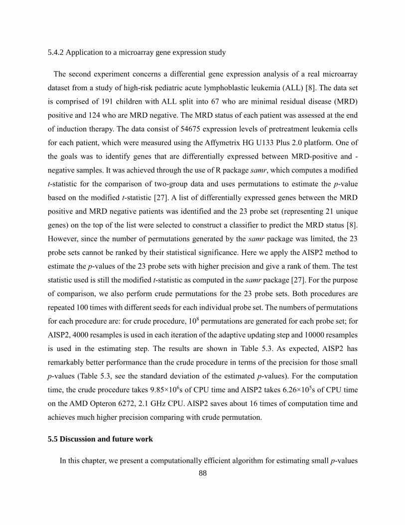
88
5.4.2 Application to a microarray gene expression study
The second experiment concerns a differential gene expression analysis of a real microarray
dataset from a study of high-risk pediatric acute lymphoblastic leukemia (ALL) [8]. The data set
is comprised of 191 children with ALL split into 67 who are minimal residual disease (MRD)
positive and 124 who are MRD negative. The MRD status of each patient was assessed at the end
of induction therapy. The data consist of 54675 expression levels of pretreatment leukemia cells
for each patient, which were measured using the Affymetrix HG U133 Plus 2.0 platform. One of
the goals was to identify genes that are differentially expressed between MRD-positive and -
negative samples. It was achieved through the use of R package samr, which computes a modified
t-statistic for the comparison of two-group data and uses permutations to estimate the p-value
based on the modified t-statistic [27]. A list of differentially expressed genes between the MRD
positive and MRD negative patients was identified and the 23 probe set (representing 21 unique
genes) on the top of the list were selected to construct a classifier to predict the MRD status [8].
However, since the number of permutations generated by the samr package was limited, the 23
probe sets cannot be ranked by their statistical significance. Here we apply the AISP2 method to
estimate the p-values of the 23 probe sets with higher precision and give a rank of them. The test
statistic used is still the modified t-statistic as computed in the samr package [27]. For the purpose
of comparison, we also perform crude permutations for the 23 probe sets. Both procedures are
repeated 100 times with different seeds for each individual probe set. The numbers of permutations
for each procedure are: for crude procedure, 108 permutations are generated for each probe set; for
AISP2, 4000 resamples is used in each iteration of the adaptive updating step and 10000 resamples
is used in the estimating step. The results are shown in Table 5.3. As expected, AISP2 has
remarkably better performance than the crude procedure in terms of the precision for those small
p-values (Table 5.3, see the standard deviation of the estimated p-values). For the computation
time, the crude procedure takes 9.85×10⁶s of CPU time and AISP2 takes 6.26×10⁵s of CPU time
on the AMD Opteron 6272, 2.1 GHz CPU. AISP2 saves about 16 times of computation time and
achieves much higher precision comparing with crude permutation.
5.5 Discussion and future work
In this chapter, we present a computationally efficient algorithm for estimating small p-values

89
from permutation tests using the adaptive cross-entropy method. Simulation studies and analysis
of a real microarray dataset show that our approach achieves significant gains in computational
efficiency comparing with existing methods. We should also note that the statistics used in our
examples are very simple, and thus takes less amount of time to compute comparing with the time
of generating the permutated samples. If the test statistics used in the permutation tests are
relatively complicated, the crude procedure and SAMC will take even longer time, since both the
two procedures need much more permutated samples than AISP2.
As we see in the second simulation example with 100k m , one issue with the current
implementation of the adaptive importance sampling method is that the variances of the estimated
p-values increase with the sample sizes. The underlying reason for that issue is the number of
parameters to be updated grows with sample sizes and the likelihood ratios involving in the
importance sampling become more and more unstable with the number of parameters growing,
which has been known as the “curse of dimensionality” of the likelihood ratios when using IS in
high dimensional Monte Carlo simulations [122]. Several methods have been introduced to deal
with that problem. One method specifically dealing with the degeneracy of the likelihood ratios in
adaptive CE method is called the “screening method”, which first identifies a subset of the
parameters that have most significant effects in high dimensional Monte Carlo simulations and
then only updates that subset of parameters via adaptive CE method [122]. As future work, we will
consider of using this type of dimension reduction approaches in our method to reduce the variance
in high-dimension problems.
A natural extension of this work is to extend the current adaptive importance re-sampling
approach for one-group and unpaired two-group data to multiple-group data. To that end, we need
to parameterize the permutation sample space of multiple-group data by some distributions as we
have done with one-group and unpaired two-group data. One direction is to sequentially applying
the CB distribution to multiple groups. For instance, if we have three groups, we can first consider
the second and third groups as one single group, and then select elements for the first group by the
CB distribution, and then select elements for the second group using the CB distribution again,
and the remaining unselected elements are assigned to the third group. Hence, the density of the
distribution parameterizing the permutation sample space of the three-group data is the product of
density of two CB distributions. We consider this extension as our future work.

90
Table 5.1 Performance of different algorithms on the first two-group permutation test example.
k = m = 20 Each procedure is repeated 100 times with different seeds
x1 x2 Crude I Crude II
�̂� MSE ARE MCRE #samples (time) �̂� MSE ARE MCRE #samples (time)
N(1, 1) N(0, 1) 6.70×10⁻⁵ 5.81×10⁻¹³ - 1.14×10⁻³ 108 (2.23×10⁵) 6.72×10⁻⁵ 5.28×10⁻¹² 2.46×10⁻³ 3.44×10⁻³ 107 (2.29×10⁴)
N(1.25, 1) N(0, 1) 4.76×10⁻⁶ 4.81×10⁻¹⁵ - 1.47×10⁻³ 109 (2.40×10⁶) 4.77×10⁻⁶ 5.01×10⁻¹⁴ 2.79×10⁻³ 4.72×10⁻³ 108 (2.12×10⁵)
N(1.5, 1) N(0, 1) 3.67×10⁻⁷ 3.01×10⁻¹⁷ - 1.50×10⁻³ 1010 (1.97×10⁷) 3.68×10⁻⁷ 3.63×10⁻¹⁶ 2.13×10⁻³ 5.21×10⁻³ 109 (2.17×10⁶)
AISP2 SAMC
�̂� MSE ARE MCRE #samples (time) �̂� MSE ARE MCRE #samples (time)
6.67×10⁻⁵ 2.01×10⁻¹² 4.36×10⁻³ 2.08×10⁻³ 1.6×10⁴ (9.04×10²) 6.62×10⁻⁵ 1.20×10⁻¹¹ 1.27×10⁻² 5.03×10⁻³ 1.2×10⁶ (6.72×10⁴)
4.71×10⁻⁶ 1.44×10⁻¹⁴ 1.02×10⁻² 2.32×10⁻³ 1.8×10⁴ (2.43×10³) 4.66×10⁻⁶ 4.95×10⁻¹⁴ 2.08×10⁻² 4.21×10⁻³ 1.2×10⁶ (6.72×10⁴)
3.68×10⁻⁷ 7.34×10⁻¹⁷ 1.90×10⁻³ 2.34×10⁻³ 1.8×10⁴ (2.44×10³) 3.63×10⁻⁷ 4.35×10⁻¹⁶ 1.23×10⁻² 5.57×10⁻³ 1.2×10⁶ (6.97×10⁴)
The meanings of each column:
N(µ, σ) means the sample is drawn from a normal distribution with mean µ and standard deviation σ.
p̂ : this is the average of the estimated p-values from 100 runs of each algorithm, where p̂ from Crude I method is used as the underlying true p-value in the following
calculation of errors.
MSE: mean square error, defined as 2
1
1ˆ( )
N
iip p
N , where ˆ
ip is the estimated p-value from the ith ( 1,...,100i ) run, p is the underlying true p-value and N is 100.
ARE: absolute relative error, defined as ˆ| ( ) / |p p p , where p̂ is the average of the 100 estimated p-values from 100 runs of each algorithm.
MCRE: Monte Carlo relative error, defined as /S N
p, where S is the sample standard deviation of the 100 estimated p-values from 100 runs of each procedure.
#samples: this is the total number of permutated samples used for one single run of each algorithm. For SAMC, we used default values of the program, i.e. 2×10⁵ resamples
for refining the partitions of the test statistic and 106 resamples for the final step of estimating the p-value.
time: this is the CPU time in seconds of 100 runs on a cluster with 64 cores of AMD Opteron 6272, 2.1 GHz CPU (For Crude I method with 1010 permutations, we split
the jobs on two clusters. The time reported here is the sum of CPU time with 60 runs on 60 cores of AMD Opteron 6272, 2.1 GHz CPU and 40 runs on 40 cores of AMD
8214, 2.2 GHz).

91
Table 5.2 Performance of different algorithms on the second two-group permutation test example.
k = m = 100 Each procedure is repeated 100 times with different seed
x1 x2 AISP2 SAMC I SAMC II
�̂� (S.D.*) #samples (time) �̂� (S.D.*) #samples (time) �̂� (S.D.*) #samples (time)
N(0.5, 1) N(0, 1) 9.54×10⁻⁷
(3.69×10⁻⁸)
3.6×10⁴
(2.71×10⁴)
9.58×10⁻⁷
(2.60×10⁻⁸)
5.2×10⁶
(3.03×10⁵)
9.45×10⁻⁷
(5.60×10⁻⁸)
1.2×10⁶
(7.80×10⁴)
N(0.6, 1) N(0, 1) 2.62×10⁻⁸
(4.35×10⁻⁹)
3.6×10⁴
(3.34×10⁴)
2.65×10⁻⁸
(8.37×10⁻¹⁰)
5.2×10⁶
(3.03×10⁵)
2.60×10⁻⁸
(1.71×10⁻⁹)
1.2×10⁶
(8.02×10⁴)
N(0.65, 1) N(0, 1) 3.64×10⁻⁹
(1.11×10⁻⁹)
**4×10⁴
(4.16×10⁴)
3.89×10⁻⁹
(1.39×10⁻¹⁰)
5.2×10⁶
(3.03×10⁵)
3.82×10⁻⁹
(2.66×10⁻¹⁰)
1.2×10⁶
(8.07×10⁴)
N(0.7, 1) N(0, 1) 5.13×10⁻¹⁰
(2.47×10⁻¹⁰)
4×10⁴
(4.18×10⁴)
5.41×10⁻¹⁰
(2.09×10⁻¹¹)
5.2×10⁶
(3.03×10⁵)
5.19×10⁻¹⁰
(4.27×10⁻¹¹)
1.2×10⁶
(8.14×10⁴)
*S.D.: this is the sample standard deviation of the estimated p-values from 100 runs of each algorithm. The meanings of the rest columns are the
same as Table 4.1.
**Among the 100 runs in this simulation, one single run reach the target threshold value after 5 iterations, and the rest 99 runs all take 4 iterations.
So the total number of resamples for that single run is 4×10⁴ and the rest is 3.6×10⁴.
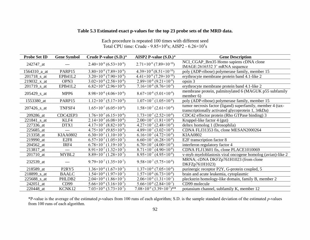
92
Table 5.3 Estimated exact p-values for the top 23 probe sets of the MRD data.
Each procedure is repeated 100 times with different seed
Total CPU time: Crude - 9.85×10⁶s; AISP2 - 6.26×10⁵s
Probe Set ID Gene Symbol Crude P-value (S.D.)* AISP2 P-value (S.D.)* Gene Description
242747_at --- 2.40×10⁻⁹ (6.53×10⁻⁹) 2.71×10⁻⁹ (7.89×10⁻¹⁰) NCI_CGAP_Brn35 Homo sapiens cDNA clone IMAGE:2616532 3’ mRNA sequence
1564310_a_at PARP15 3.80×10⁻⁹ (7.89×10⁻⁹) 4.39×10⁻⁹ (8.51×10⁻¹⁰) poly (ADP-ribose) polymerase family, member 15
201718_s_at EPB41L2 3.20×10⁻⁹ (7.90×10⁻⁹) 4.41×10⁻⁹ (7.29×10⁻¹⁰) erythrocyte membrane protein band 4.1-like 2 219032_x_at OPN3 3.02×10⁻⁸ (2.58×10⁻⁸) 2.89×10⁻⁸ (9.21×10⁻⁹) opsin 3 201719_s_at EPB41L2 6.82×10⁻⁸ (2.96×10⁻⁸) 7.16×10⁻⁸ (8.76×10⁻⁹) erythrocyte membrane protein band 4.1-like 2
205429_s_at MPP6 8.98×10⁻⁸ (4.06×10⁻⁸) 8.67×10⁻⁸ (5.01×10⁻⁹) membrane protein, palmitoylated 6 (MAGUK p55 subfamily member 6)
1553380_at PARP15 1.12×10⁻⁷ (5.17×10⁻⁸) 1.07×10⁻⁷ (1.05×10⁻⁸) poly (ADP-ribose) polymerase family, member 15
207426_s_at TNFSF4 1.65×10⁻⁷ (6.05×10⁻⁸) 1.58×10⁻⁷ (2.61×10⁻⁸) tumor necrosis factor (ligand) superfamily, member 4 (tax-transcriptionally activated glycoprotein 1, 34kDa)
209286_at CDC42EP3 1.76×10⁻⁷ (6.15×10⁻⁸) 1.73×10⁻⁷ (2.52×10⁻⁸) CDC42 effector protein (Rho GTPase binding) 3 221841_s_at KLF4 2.14×10⁻⁷ (6.08×10⁻⁸) 2.00×10⁻⁷ (1.81×10⁻⁸) Kruppel-like factor 4 (gut) 227336_at DTX1 4.17×10⁻⁷ (8.82×10⁻⁸) 4.27×10⁻⁷ (2.48×10⁻⁸) deltex homolog 1 (Drosophila) 225685_at --- 4.75×10⁻⁷ (9.85×10⁻⁸) 4.89×10⁻⁷ (3.02×10⁻⁸) CDNA FLJ31353 fis, clone MESAN2000264 213358_at KIAA0802 6.30×10⁻⁷ (1.10×10⁻⁷) 6.16×10⁻⁷ (4.72×10⁻⁸) KIAA0802 219990_at E2F8 6.57×10⁻⁷ (1.05×10⁻⁷) 6.60×10⁻⁷ (6.28×10⁻⁸) E2F transcription factor 8
204562_at IRF4 6.78×10⁻⁷ (1.19×10⁻⁷) 6.70×10⁻⁷ (4.00×10⁻⁸) interferon regulatory factor 4 213817_at --- 8.91×10⁻⁷ (1.32×10⁻⁷) 8.71×10⁻⁷ (4.90×10⁻⁸) CDNA FLJ13601 fis, clone PLACE1010069 201710_at MYBL2 8.89×10⁻⁷ (1.28×10⁻⁷) 8.95×10⁻⁷ (4.95×10⁻⁸) v-myb myeloblastosis viral oncogene homolog (avian)-like 2
232539_at --- 9.79×10⁻⁷ (1.35×10⁻⁷) 9.58×10⁻⁷ (5.75×10⁻⁸) MRNA; cDNA DKFZp761H1023 (from clone DKFZp761H1023)
218589_at P2RY5 1.36×10⁻⁶ (1.67×10⁻⁷) 1.37×10⁻⁶ (7.05×10⁻⁸) purinergic receptor P2Y, G-protein coupled, 5 218899_s_at BAALC 1.54×10⁻⁶ (1.97×10⁻⁷) 1.57×10⁻⁶ (6.73×10⁻⁸) brain and acute leukemia, cytoplasmic
225688_s_at PHLDB2 2.04×10⁻⁶ (1.86×10⁻⁷) 2.06×10⁻⁶ (1.31×10⁻⁷) pleckstrin homology-like domain, family B, member 2 242051_at CD99 5.66×10⁻⁶ (3.16×10⁻⁷) 5.66×10⁻⁶ (2.84×10⁻⁷) CD99 molecule 220448_at KCNK12 7.03×10⁻⁶ (3.73×10⁻⁷) 7.08×10⁻⁶ (3.39×10⁻⁷)** potassium channel, subfamily K, member 12
*P-value is the average of the estimated p-values from 100 runs of each algorithm; S.D. is the sample standard deviation of the estimated p-values
from 100 runs of each algorithm.

93
**For this probe set, there is one outlier with p-value of 2.81×10⁻⁵ among the 100 runs of AISP2. For that single run, the adaptive updating step does
not reach the target threshold value after 20 iterations. The p-value and S.D. for this probe set in the table are based on the 99 runs with that outlier
removed. The estimated p-value and SD based on all the 100 runs are 7.29×10⁻⁶ (2.13×10⁻⁶).

94
CHAPTER VI
Efficient estimation of small p-values in parametric bootstrap tests using
Hamiltonian Monte Carlo cross-entropy method
The bootstrap tests as we discussed in Chapter IV for analyzing single-cell high-throughput gene
expression data, together with permutation tests, are two types of resampling methods that are
widely used when the asymptotic distribution of the test statistic is unavailable or unreliable due
to small sample sizes. Similar to permutation tests as we discussed in Chapter V, bootstrap tests
suffer from the issue of high computational burden when it is required to obtain reliable estimations
of small p-values. In this chapter, we focus on parametric bootstrap tests and develop an algorithm
for efficient estimation of small p-values in parametric bootstrap tests. Our approach not only uses
the principle of the cross-entropy method that we discussed in Chapter V to approximate the
optimal proposal density, but also incorporates the Hamiltonian Monte Carlo method to efficiently
sample from the optimal proposal density. Our new method avoids the adaptive updating step in
the classical adaptive cross-entropy method and hence considerably improves the computational
efficiency. We apply our method to the problem of testing the variance component in linear mixed-
effects models with demonstrations through simulations and an analysis of gene set differential
expression with a microarray dataset. Our approach achieves considerable gains in computational
efficiency when compared with the standard parametric bootstrap procedure.
6.1 Introduction
We first briefly discuss the general parametric bootstrap test procedure in this section. Suppose
our goal is to test a null hypothesis H0 versus an alternative hypothesis H1 using a test statistic
T(•), which is constructed under a parametric model (e.g., the linear mixed-effects model as we
discuss below in Section 6.3). Let γ be the observed test statistic, then the p-value is defined as

95
0Pr |( )p T H . Parametric bootstrap tests are widely used to estimate the p-value when the
asymptotic distribution of the test statistic is unavailable or unreliable due to small sample sizes
[101-103,123-125]. It first fits the model under H0 (denoted as0
ˆHf below) and then computes
the p-value by simulating data from 0
ˆHf . The procedure is usually performed in the following
way [102,103]:
Procedure 1 (The general parametric bootstrap test method)
(1) Generate N (for e.g., N = 10,000) random samples 1,..., Ny y from 0
ˆHf .
(2) Calculate the corresponding test statistics 1 ,( ) ), ( NT Ty y with the simulated samples
1,..., Ny y .
(3) Estimate the p-value as 1
1ˆ { ( ) }
N
l
l
p I TN
y (an alternative formula is
1
{ ( ) } 1
ˆ1
N
l
l
I T
pN
y
. The two formulas give almost the same result providing N is large, so
we use the former throughout this chapter).
The above parametric bootstrap test procedure, similar to permutation tests, suffers from the
same issue of high computational burden when it is required to obtain reliable estimation of small
p-values, which is a common situation in genomic problems as we discussed in Chapter V. This
motivates us to develop new methods to improve computational efficiency for parametric
bootstrap tests. In this chapter, we propose a new algorithm that can dramatically reduce the
computational time for estimating small parametric bootstrap p-values by combing the cross-
entropy method that we discussed in Chapter V and the Hamiltonian Monte Carlo method. In the
following sections, we first briefly review the principle of cross-entropy method within the
framework of parametric bootstrap, and then we introduce our new approach. Next, we apply our
method to the problem of testing the variance component in linear mixed-effects models using
parametric bootstrap, and then demonstrate its performance by simulations and an analysis of gene

96
set differential expression with a microarray dataset. We close this chapter with discussions on
possible extensions of the current approach.
6.2 Methods
6.2.1 Estimating small parametric bootstrap p-values using cross-entropy method
From the above discussions, we can easily see that the parametric bootstrap test is essentially a
Monte Carlo sampling procedure, and the problem of estimating small p-values using the
parametric bootstrap test is equivalent to estimating the small probability 0Pr[ ( ) | ]T Hy by
drawing random samples y from the null model 0
ˆHf . As we discussed in Chapter V, the cross-
entropy (CE) method [111] can be used to efficiently estimate small probabilities in Monte Carlo
procedures by updating the parameters of the probability distribution via importance sampling.
From hereafter we will use 0( ; )f θ to represent probability distribution of the data under the null
model 0
ˆHf to emphasize that 0θ is the parameter of the null model. For instance, for parametric
bootstrap tests in linear mixed-effects models (LMMs) to which we will apply our method (Section
6.3 below), 0( ; )f θ is a multivariate normal distribution and 0θ contains the mean and covariance
of that multivariate normal distribution.
Here, we briefly review the CE method under the parametric bootstrap framework. Similar to
our discussions in Chapter V, the p-value in parametric bootstrap tests is defined as
0 0Pr [ ( ) ] [ { ( ) }]p T E I T
θ θy y (6.1)
and can be estimated by its stochastic counterpart 1
1ˆ { ( ) }
N
l
l
p I TN
y [111], where 1,..., Ny y
are random samples drawn from 0( ; )f θ . Applying the CE method to estimate the above p-value
defined in equation (6.1) essentially follows our discussions in Section 4.2 of Chapter V: let g(•)
be the proposal density, then by the importance sampling method, p can be written as
0 0( ; ) ( ; ){ ( ) } ( )d [ { ( ) } ]
( ) ( )g
f fp I T g E I T
g g
y θ y θy y y y
y yY (6.2)

97
and hence can be estimated by the stochastic counterpart of (6.2):
0
1
1 ( ; )ˆ { ( ) }
( )
N
l
l l
fp I T
N g
y θ
yy
(6.3)
where the subscript g in equation (6.2) indicates that the expectation is taken with respect to the
proposal density g(•), and 1,..., Ny y in equation (6.3) are random samples drawn from g(•). The
optimal proposal density [111,114] is
* 0{ ( ) } ( ; )( )
I T fg
p
y y θy (6.4)
The adaptive CE method [111] provides one way of finding a proposal density ( ; )f θ that is
close to the optimal proposal density *g within the same distribution family as 0( ; )f θ by
minimizing the cross-entropy between *g and ( ; )f θ , which is defined as
** *
* * *
( )( ), : ( ) ln d
( ) ln ( )d ( ) l
;
d;n
•;ff
gg
g g f
g
g
yθ y y
y θ
y y y y y θ y
y
y y
D (6.5)
The first term in the right-hand side of equation (6) does not depend on θ and the second term
can be written as
0
0( ; )
{ ( ) } ( ; ) 1ln d [ { ( ) }ln; ];f
I T fE I T
pf f
p
θ
y y θy θ y y y θ
y
Therefore, the parameter θ that minimizes *( ), •;g f θD is the solution to the following
optimization problem:
0( ; ) ;argmax [ { ( ) }ln ]fE I fT θ
θ
y y θ (6.6)
Following our discussions in Section 4.2 of Chapter V and [111], problem (6.6) can be solved
adaptively using the following procedure:
Procedure 2 (The adaptive CE method for rare-event probability estimation)
A. Adaptive updating step:
(1) Specify a constant 0,1 . Start with parameter 0θ ; Set the iteration counter k = 0.

98
(2) At the kth iteration, generate random samples 1,..., Ny y from ( ; )kf θ . Calculate the statistics
1 ,( ) ), ( NT Ty y , and compute k as their sample (1 ) quantile, provided k . If k ,
set k .
(3) Updating the parameter kθ with 1kθ , which is the solution to the following problem:
01
1
1 ( ; )arg max [ { ( ) } ln ( ; )]
( ; )
Nl
k l k l
l l k
fI T f
N f
θ
y θθ y y θ
y θ
(4) If k , set k = k+1 and reiterate from Step (2); otherwise, proceed to the following Step B.
B. Estimating step:
Use ( ; )kf θ as the proposal density and generate random samples 1,..., My y from ( ; )kf θ .
Estimate p-value as 0
1
1 ( ; )ˆ [ { ( ) } ]
( ; )
Ml
l
l l k
fp I T
M f
y θ
yy θ
.
6.2.2 Limitations of the adaptive CE method
As we implement the above adaptive CE method for estimating small p-values in parametric
bootstrap tests, we found that it does not perform very well: the algorithm either fails to converge
in some cases, or the estimated results from the converged cases show very large variations (See
the summary of the simulations in Section 6.3.2). This observation is consistent with several other
studies, which have also shown that the adaptive CE method for rare event simulation can fail in
high-dimensional settings [119,122,126,127]. As discussed in [127], one important reason for the
failure of the adaptive CE method is that the proposal density obtained from the adaptive CE
method can be far from the optimal proposal density in high dimensions, and thus is suboptimal
[127]. To overcome this problem, Chan el al developed a new approach that considerably improve
the adaptive updating procedure in terms of both accuracy and computational time [127], which is
essentially the underlining theoretical basis for our proposed method for estimating small p-values
in parametric bootstrap tests. Below we briefly show that how that approach is derived following
[127]. By re-examination of the definition of CE in equation (6.5), we can see that the second term
on the right hand side can also be re-written in the following way:
*
*( ) ln d [ln; ];g
g f E f y y θ y y θy
(6.7)

99
where the subscript *g in (6.7) means that the expectation is taken with respect to the optimal
proposal density *g . Hence the parameter θ that minimizes *( ), •;g f θD should maximize
(6.7), which is the solution to the following optimization problem:
*argmax [ n ];lg
fEθ
y θ (6.8)
Suppose we can directly draw random samples from *g (in the next section we will describe
several methods to achieve this goal), then problem (6.8) can be solved by maximizing the
stochastic counterpart of *[ln ; ]g
E f y θ , i.e.
1
1argmax [ln ];
N
llNf
θ
y θ (6.9)
where 1,..., Ny y in (6.9) are random samples drawn from *g . After dropping the constant 1
N ,
problem (6.9) can be written as
1
argmax [ln ];N
llf
θ
y θ (6.10)
which is, notably, the maximum likelihood estimation (MLE) of θ under the likelihood function
;f θ with 1,..., Ny y drawn from *g . Compared with the adaptive CE method (Procedure 2),
problem (6.10) does not contain any likelihood ratio or indicator functions, and it is a regular
problem of finding MLE in statistics, which can be solved either analytically for many commonly
used distributions [e.g., if ;f θ is a multivariate normal distribution], or numerically by widely
used approaches such as Newton-Raphson or the EM algorithm for other complicated distributions
[128].
6.2.3 Sampling from the optimal proposal density
In this section, we briefly review the algorithms for sampling from the optimal proposal density
*g . From equation (6.4), we can see that *g is a truncated distribution with the probability
distribution 0( ; )f y θ truncated by the constraint ( )T y . In the literature, there are at least three
sampling algorithms proposed for sampling from a truncated distribution in the form of *g : the
Gibbs sampler, the hit-and-run sampler and the Hamiltonian Monte Carlo sampler and all these

100
methods are based on Markov chain Monte Carlo (MCMC). The Gibbs sampler is a classical
method for drawing random samples from truncated distributions that consists of sampling from a
sequence of conditional distributions, and the details of this approach can be found in [129,130].
The hit-and-run sampler is another algorithm that can reduce the problem of sampling from a
multivariate distribution with a high dimensional constraint (such as *g ) to the problem of sampling
from a univariate truncated distribution, and the details of this algorithm can be found in [119,131].
The Hamiltonian Monte Carlo (HMC) sampler is a more recently developed algorithm that uses
principle of the Hamiltonian dynamics in physics and has become a powerful tool for sampling
from many complicated distributions [132-134], and in the following we review the core idea of
this method. As a concrete example, we consider ;f θ as a multivariate normal distribution
( , )nN μ Σ , where μ is the mean vector and Σ is the covariance matrix, and our discussion mainly
follows [135]. First note that if ~ ( , )nNy μ Σ , then y can be written as the following linear
transformation with respect to the random vector x
1/2 y μ UΛ x (6.11)
where x follows the standard multivariate normal distribution ( , )nN 0 I and
1/2 1/2( )T T Σ UΛU UΛ UΛ is the eigen-decomposition of the covariance matrix Σ and the
columns of U are unit eigenvectors and Λ is a diagonal matrix of the eigenvalues. Hence, our
following discussion will focus on how to apply HMC to sample from the truncated distribution
with respect to ( , )nN 0 I , then sampling from the truncated distribution with respect to ( , )nN μ Σ
is straightforward by applying the linear transformation (6.11) [135].
Following [135], the log density function of ( , )nN 0 I can be written as the following form:
1log ( )
2
Tf c x x x (6.12)
where c is a constant with respect to x. The HMC is a “particle method” and we need to imagine
the trace of the positions of the consecutive draws of the random samples is like a trajectory of a
particle travelling according to a potential energy function (which is determined by the probability
density function) and a kinetic energy function (which is usually introduced artificially to construct
the Hamiltonian system). The potential energy is determined by the position of the particle and the
kinetic energy is determined by the momentum of the particle, and the sum of the potential energy

101
function and the kinetic energy function is a Hamiltonian system [132-134]. For the standard
multivariate normal distribution, we can construct the following Hamiltonian
( , ) ( ) ( )H U K sx sx (6.13)
where 1
( ) log ( )2
TU f x x x x is the potential energy function (the constant c dropped) and
1( )
2
TK s s s is the artificially introduced kinetic energy function with 1( ,..., )ns ss as the vector
of momentum variables [135,136]. Based on the Hamiltonian (6.13), the evolvement of the particle
is determined by the following systems of equations according to the Newton's Laws of Motion
[135,136]
ii
i
i
i
i
dx Hs
dt s
ds Hx
dt x
(6.14)
where ix and is denote the ith element of x and s and i = 1,…, n. The two first order differential
equations in (6.14) can be combined to one equation (note that there are n such equations)
2
2, 1,...,i
i
d xx i n
dt (6.15)
which has the following analytical solution
( ) sin( ) cos( ), 1,...,i i ix t a t b t i n (6.16)
with the constants ia and ib determined by the initial conditions (discussed below) as
0
(0)
(0)
iii
t
i i
dxa s
dt
b x
(6.17)
Following [135], the HMC algorithm iterates with the following two steps: Step 1. Sample the
initial momentum variables s from ( , )nN 0 I . Step 2. Use the s from Step 1 and the values of x at
the end of last iteration as initial conditions to determine the constants ia and ib according to
equation (6.17), and then let the particle to travel for a time T. It is shown in [135] that by
constructing the HMC algorithm in the above way, the two properties of the Hamiltonian dynamics,
the conservation of energy and the conservation of volume in phase space are met and the detailed

102
balanced condition of the Markov chain Monte Carlo is satisfied. The authors of [135] also show
that a good choice of the travelling time T is / 2 .
Next consider the constraint
( )T y , (6.18)
and we imagine that it is like a wall on the trajectory of the particle. Once the particle hits the wall,
we let it bounce off the wall and continue travelling with a reflected velocity [135]. The hitting of
the wall occurs when the inequality (6.18) is saturated (i.e. takes the equality) [135], and the time
of hitting can be found by solving the following equation
[ ( )]T t y (6.19)
where y(t) is a function of time t that is determined by (6.16) and the linear transformation (6.11).
The authors of [135] give analytical solutions for (6.19) under the constraints where T(•) is linear
or quadratic functions of y. In summary, the HMC algorithm for sampling from a truncated
multivariate normal distribution iterates with the following two steps [135]:
(1) Sample the initial momentum variables s from ( , )nN 0 I .
(2) Use the s from step (1) and the values of x at the end of last iteration as initial conditions to
determine the constants ia and ib in equation (6.17), and then let the particle to travel for a time
T. During time T, if the particle hits the wall [i.e. constraint (6.18), and the time of hitting is
determined by equation (6.19)], then let it continue travelling with a reflected velocity.
For other types of continuous distributions, the HMC sampler can be constructed in a similar
way as the multivariate normal distributions discussed above, but equation (6.14) usually do not
have analytical solutions and need to be solved using some numerical methods, such as the leapfrog
algorithm for which the time is discretized with some small step size ε for L steps [132,134,136],
and details can be found in [134,136,137]. For discrete distributions, the HMC sampler can be
constructed using the technique Gaussian augmentation (or exponential augmentation) by
introducing auxiliary variables that follow Gaussian (or exponential) distributions, and details can
be found in [138,139].
As a note for the three MCMC sampling algorithms mentioned above, the authors of [135]
compare the performance of the HMC sampler and the Gibbs sampler and find that the HMC
sampler is much more efficient, since the runtime of the Gibbs sampler increase linearly with the
dimensions and it is very slow when the constraint like (6.18) “imposes high correlations among

103
coordinates” [135]. Comparisons of the performance between the hit-and-run sampler and the
HMC sampler is of our future interest, but some studies note that the hit-and-run sampler suffers
a similar problem of slow convergence in the cases where the constrained sample space impose
high correlations [135,140].
Combining the above discussions, the complete algorithm for the estimation of small p-values
in parametric bootstrap tests can be summarized below:
Procedure 3 (MCMC cross-entropy method for parametric bootstrap tests – MCMC-CE)
A. Parameters updating step:
1. Generate N random samples 1,..., Ny y from the optimal proposal density *g using one of the
MCMC sampling approaches described above (for e.g., the HMC sampler).
2. Solve the maximization problem (6.10) with 1,..., Ny y and obtain the proposal density •;f θ .
B. Estimating step:
Use •;f θ as the proposal density and generate M random samples 1,..., Ny y from •;f θ .
Estimate p-value as 1
01 ( ; )ˆ { ( ) }
( ; )
Ml
l
l l
fp I T
M f
θ
yy θ
y.
Compared with the adaptive CE method (Procedure 2), the MCMC-CE method (Procedure 3)
finds the proposal density by drawing samples from *g and solve the maximization problem (6.10)
in a single step instead of in an adaptive fashion through multiple steps. Therefore, it not only
considerably improves computational efficiency, but also gives more robust and numerically stable
estimations, as noted and studied in [127].
6.3 Application: parametric bootstrap tests for variance components in LMMs
We apply our MCMC-CE approach to the problem of testing the variance components in LMMs
using parametric bootstrap. Following the notations in [141], we consider the LMMs of the
following form:
2~ N { , ( )}n Y Xβ V τ
with
1( )
J
j jj
V τ I K , (6.20)
where Y is an n × 1 vector of data following the multivariate normal distribution with mean Xβ

104
and variance σ2V(τ), X is an n × p design matrix for covariates (fixed effects), β is a p × 1 vector
of fixed-effect parameters, I is the n × n identity matrix, Kj’s, j = 1,…, J, are n × n known positive
semidefinite matrices, σ2 is the variance parameter for the error term, τj’s, j = 1,…, J, are the scaled
variance component parameters such that σ2τj is the jth variance component [141]. This form of
LMMs are widely used for analyzing a variety types of data in practice. For instance, in multi-
level random effect models Kj is given by T
j jΖ Z , where Zj is an n × qj design matrix for the jth
random effect factor [99,141]. In genomic studies, Liu et al develops a method for testing the
association between a gene set/pathway (i.e. a group of genes with relevant biological functions)
and a continuous outcome using the LMM representations of linear-square kernel machine [107].
In their model, the effect of a gene set/pathway is modeled non-parametrically using a kernel
function and can be represented by a single variance component LMM [i.e. J =1 written in the
form of model (11)], where the matrix K1 corresponds to the kernel matrix [107]. Nowadays this
type of models are also widely used in genome-wide association studies (GWAS) to test the
associations between a phenotype and a set of common and rare single nucleotide polymorphisms
(SNPs) [142,143].
In all the applications discussed above, the goal is to test the significance of a single variance
component, which can be written as the following hypothesis test problem:
0 : 0jH v.s. 1 : 0jH (6.21)
for the jth variance component. In genomic studies, the score-type statistic of the form
( ) ( )T
jT Y Xβ K Y Xβ (6.22)
proposed by Lin and colleagues has attracted considerable attention [107,141-143]. The score
statistic (6.22) is computed under the null model that has fewer variance component parameters
than the alternative model, and hence can reduce the computational time considerably compared
with other types of tests such as the likelihood ratio test, so that it has been widely used in high-
throughput genomic studies, for which the computational burden is often significant [107,142,143].
In the literature, several methods have been used to approximate the distribution of T under H0,
such as the Satterthwaite method [107] or the Davies method [141-144]. As noted in [143], for
large sample studies these methods perform generally well for controlling type I error rate and
achieving adequate power, but when the sample size is small, the type I error rate is often not well-
controlled at genome-wide small α levels (e.g. <10-6) [143]. Hence, resampling-based approaches

105
are recommended for that situation, which can correctly control the type I error rate [143]. Below
we use the parametric bootstrap to estimate the p-value using the score statistic (6.22) and show
how our MCMC-CE method can be used to efficiently reduce the computational time.
6.3.1 Test the variance component for LMMs with a single variance component
In LMMs with a single variance component, to test the variance component τ (we drop the
subscript j in this section, since there is only one variance component), note that under the null
model H0, 0( ; )f θ is a multivariate normal distribution of the form (6.20) with 2
0 0 0( , )Tθ Xβ ,
and the parameters β0 and 2
0 are estimated under the null model H0 (the subscript ‘0’ is to
emphasize that fact), which is a regular linear regression model, and 0V τ is simply the identity
matrix I with no unknown parameters. Implementation of the general parametric bootstrap test
(Procedure 1) is straightforward by first estimating parameters β0 and 2
0 and computing the
observed score statistic γ according to equation (6.22) and then simulating data from the null model
2
0 0ˆ ˆN { , }n Xβ I following Procedure 1.
To apply the MCMC-CE method, note that under the null model β0 is estimated by
1
0ˆ ( )T Tβ X X X Y , hence the constraint ( )T y can be written as
1 1[ ( ) ] [ ( ) ]T T T T T Y X X X X Y K Y X X X X Y
which can be further written as the following quadratic constraint function with respect to Y :
1 1[ ( ) ] [ ( ) ] 0T T T T T T Y I X X X X K I X X X X Y (6.23)
Therefore, the optimal proposal density *g is a truncated distribution with 2
0 0ˆ ˆN { , }n Xβ I
truncated by constraint (6.23), and random samples from *g can be drawn using one of the three
MCMC algorithms reviewed in Section 6.2.3. The implementation of the MCMC-CE method
follows Procedure 3. In our applications, we use the HMC algorithm as implemented in the R
package tmg [135] to draw random samples from *g , and hence we name our approach as HMC-
CE below.
Simulations. We conduct simulation studies to compare the general parametric bootstrap test
(below named as brute-force PB) and the HMC-CE method for the variance component test in
LMMs with a single variance component. The following single-level clustered random-effect

106
model is used in the simulations:
0ij j ijY b e
with
2~ (0, )j bb N and 2~ (0, )ij ee N (6.24)
where Yij is the outcome of subject i in cluster j (i = 1,…, nj; j = 1,…, m; m is the number of clusters
and nj is the number of subjects in cluster j), bj and eij are respectively the random effect of cluster
j and the random error at subject level, 2
b and 2
e are the variances for bj and eij, and m
jjN n
is the total number of subjects. The goal is to test the significance of the variance component 2
b ,
i.e.
H0: 2 0b v.s. H1:
2 0b
If we compare model (6.24) to the alternative form in (6.20), we can see that here the matrix K is
a N × N block diagonal matrix that can be written as T
ZZ where Z is an N × m design matrix with
indicators of cluster indices denoting which subject belongs to which cluster.
In our simulations, we fix the following parameters: 0 5 , 2 1e , 6jn for all j’s, j = 1,…,
m, and tune the effect size and sample size by varying 2
b and m. In the first simulated experiment,
we fix m at m = 5 and vary b for three different values 1.75, 1.9 and 2.0 respectively, which give
different p-values on the orders of 10-5, 10-6 and 10-7 (Table 6.1). Then we use the brute-force
parametric bootstrap and the HMC-CE method to estimate the p-values in a more accurate fashion.
For the brute-force parametric bootstrap, the number of re-samples used equals to 10 divided by
the order of the three p-values, which gives 106, 107 and 108 number of re-samples (Table 6.1).
For the HMC-CE, we draw 10000 samples using the HMC method in the parameter updating step
to obtain the proposal density, and 2000 samples from the proposal density to estimate the p-values
in the estimating step (see Procedure 3). For both methods, we repeated 50 times with different
random seeds and use the average of the 50 estimated p-values as the final point estimation of the
p-values ( p̂ in Table 6.1). We also calculate the standard deviation (S.D.) for the 50 estimated p-
values and record the computational time. The results of this experiment are shown in Table 6.1.
In the second simulated experiment, we fix b at 1.3b and vary m for three different values
6, 8 and 9 respectively, then we perform exactly the same procedure as that in the first experiment.

107
The results of this experiment are shown in Table 6.2.
From Table 6.1 and Table 6.2, we can see that the brute-force parametric bootstrap and HMC-
CE give almost the same estimated p-values. In terms of precision, HMC-CE reduces the S.D.
roughly by a factor of 10 compared with the brute-force method and hence is much more accurate.
Lastly, but importantly, the HMC-CE reduces the computational time roughly by a factor ranging
from 300 to 10000 compared with the brute-force method, and the gain in computational efficiency
are more considerable as the p-value goes smaller.
In the above two numerical experiments, we also apply the adaptive CE method (Procedure 2).
We find that this method fails to converge to a close-to-optimal proposal density after reaching the
maximum number of iterations (which is set as 20 here) in approximate 30% of the times, and in
those converged cases the estimated p-values show very large variations and the average over
different repetitions (not shown here) deviates substantially from those of the brute-force PB and
the HMC-CE shown in Table 6.1 and 6.2. Though we do not know the reason for the failure of the
adaptive CE method and will further investigate this algorithm in the future, we note that our
findings are consistent with several other studies that have also shown that the adaptive CE method
has some issues in terms of robustness and numerical stability in some high-dimensional settings
[119,122,126,127].
Table 6.1 Simulation results of parametric bootstrap tests for variance component in LMMs
with a single random effect – varying effect size.
σb Brute-force HMC-CE
�̂�
(S.D.)
#samples
(time) �̂�
(S.D.)
#samples
(time)
1.75 1.58×10⁻⁵
(7.63×10⁻⁶)
106
(2.69×10⁵)
1.51×10⁻⁵
(8.38×10⁻⁷)
1.2×10⁴
(8.94×10²)
1.9 2.42×10⁻⁶
(1.57×10⁻⁶)
107
(3.42×10⁶)
2.47×10⁻⁶
(1.02×10⁻⁷)
1.2×10⁴
(1.32×10³)
2.0 7.97×10⁻⁷
(3.41×10⁻⁷)
108
(1.76×10⁷*)
7.89×10⁻⁷
(3.38×10⁻⁸)
1.2×10⁴
(1.87×10³)
*For this p-value, we split the computational jobs on two clusters and the computational time here
is the sum of CPU time in seconds with 25 runs on 64 cores of AMD Opteron 6272, 2.1 GHz CPU
and 25 runs on 80 cores of AMD 8214, 2.2 GHz. For others, the computational time is CPU time
in seconds on 64 cores of AMD Opteron 6272, 2.1 GHz.

108
Table 6.2 Simulation results of parametric bootstrap tests for variance component in LMMs
with a single random effect – varying sample size.
m Brute-force HMC-CE
�̂�
(S.D.)
#samples
(time) �̂�
(S.D.)
#samples
(time)
6 6.51×10⁻⁵
(2.78×10⁻⁵)
106
(3.71×10⁵)
6.54×10⁻⁵
(3.16×10⁻⁶)
1.2×10⁴
(1.26×10³)
8 1.09×10⁻⁶
(6.21×10⁻⁷)
107
(4.13×10⁶)
1.02×10⁻⁶
(7.34×10⁻⁸)
1.2×10⁴
(1.83×10³)
9 4.58×10⁻⁷
(2.31×10⁻⁷)
108
(2.37×10⁷*)
4.65×10⁻⁷
(2.57×10⁻⁸)
1.2×10⁴
(2.41×10³)
*For this p-value, we split the computational jobs on two clusters and the computational time here
is the sum of CPU time in seconds with 25 runs on 64 cores of AMD Opteron 6272, 2.1 GHz CPU
and 25 runs on 80 cores of AMD 8214, 2.2 GHz. For others, the computational time is CPU time
in seconds on 64 cores of AMD Opteron 6272, 2.1 GHz.
6.3.2 Test one variance component in LMMs with multiple variance components
For LMMs with multiple variance components [i.e. J ≥ 2 in model (6.20)], to test the significance
of the jth variance component τj [see formula (6.21)], note that 0( ; )f θ now is a multivariate
normal distribution with mean Xβ0 and covariance 2
0 0V τ , which is computed under the null
model H0 without τj. Also note that the matrix 0V τ contains one or more variance components
other than τj, and we use \J jτ to denote those variance components excluding τj. Implementation
of the brute-force parametric bootstrap test is again straightforward by first fitting the H0 model
2
0 0 0 \ˆ ˆˆN { , ( )}n J jXβ V τ , and then simulating data following Procedure 1.
To apply the MCMC-CE method, we need to estimate β0 first. Note that the regular generalized
least-square estimator
2 1 1 2 1
0 0 0 \ 0 0 \ˆ ˆ ˆˆ ˆ{ [ ( )] } [ ( )]T T
J j J j β X V τ X X V τ Y (6.25)
in LMMs depends on \J jτ , and all the parameters β0, \J jτ and σ0 have to be estimated iteratively
by maximizing the likelihood (or restricted likelihood) function of the LMM model [99,145].
Hence the constraint

109
0 0ˆ ˆ( ) ( )T
jT Y Xβ K Y Xβ (6.26)
cannot be written as a quadratic constraint function that solely depends on Y as in the case of single
variance component LMMs. To solve this problem, we use the following approximated method:
Since the ordinary least square estimator 1
0,ˆ ( )T T
OLS
β X X X Y is also an unbiased estimator of
β0 [146], so we use 0,ˆ
OLSβ to approximate the general least-square estimator (6.25) in LMMs, and
hence use
1 1[ ( ) ] [ ( ) ]T T T T T
OLS jT Y X X X X Y K Y X X X X Y (6.27)
to approximate the constraint (6.26). As long as OLST is not far away from T, we can still generate
random samples from a probability density function truncated by the constraint (6.27) that is close
to the optimal proposal density *g , which is named as *
ag hereafter. Therefore, *
ag is a truncated
distribution with 2
0 0 0 \ˆ ˆˆN { , ( )}n J jXβ V τ distribution truncated by the constraint (6.27), and similar
to the single variance component LMMs case, random samples from *
ag can be drawn using the
HMC sampler and the implementation of the HMC-CE method then follows with Procedure 3.
Simulations. We conduct simulation studies to compare the brute-force parametric bootstrap and
the HMC-CE method for testing one variance component in LMMs with multiple variance
components. The following two-level clustered random-effect model is used in the simulations:
0ijk i ij ijkY b b e
with
2
1~ (0, )ib N , 2
2~ (0, )ijb N and 2~ (0, )ijk ee N (6.28)
In this model, there are two levels of clustering: some small clusters (level-2 cluster) are nested in
some big clusters (level-1 cluster), and the subjects are nested in level-2 clusters [99]. The
meanings of the symbols in model (6.28) are: Yijk is the outcome of subject k in the jth level-2
cluster of the ith level-1 cluster (k = 1,…, nij; j = 1,…, mi; i = 1,…, l; l is the number of level-1
clusters; mi is the number of level-2 clusters in the ith level-1 cluster; nij is the number of subjects
in the jth level 2 cluster of the ith level 1 cluster), bi, bij and eijk are respectively the two random
effects correspond to level-1 cluster, level-2 cluster and the random error at subject level, 2
1 , 2
2
and 2
e are the variances of bi, bij and eijk, and i
i
l m
ijm jN n is the total number of

110
observations. The goal is to test the significance of the variance component 2
2 , i.e.
H0: 2
2 0 v.s. H1: 2
2 0
Suppose Yijk’s are ordered according to the indices of clusters (first by the indices of level-1 cluster,
then by the level-2 cluster), then if we compare model (6.28) to its alternative form (6.20), we can
see that here the matrix K2 (the subscript 2 means we are testing the 2nd variance component 2
2 )
is a N × N block diagonal matrix that can be written as T
ZZ with Z as an ( )l
iiN m design matrix
with indicators of level-2 cluster indices denoting which subject belongs to which level-2 cluster.
In our simulations, we fix the following parameters: 0 1 ,
1 1 , 0.5e , 5l , 5im for
all i’s, 4ijn for all i’s and j’s (j = 1,…, mi; i = 1,…, l), and tune the effect size by varying the
parameter σ2 at three different values 0.375, 0.4 and 0.45 respectively, which give different p-
values on the orders of 10-5, 10-6 and 10-7 (Table 6.3). Then we use the brute-force parametric
bootstrap and the HMC-CE method to estimate the p-values similarly as that in the single variance
component LMM case, and for both methods the numbers of re-samples and repetitions, and the
summary statistics calculated (point estimation of the p-values, S.D. and time) are the same as in
Section 6.3.1. The results of this experiment are shown in Table 6.3.
From Table 6.3, we can see that the brute-force parametric bootstrap and HMC-CE give almost
the same estimated p-values. In terms of precision, HMC-CE reduces the S.D. roughly by a factor
of 6 compared with the brute-force method (note that here the variations of the HMC-CE increase
a bit compared with the single random-effect LMM case, since we use *
0g to approximate the
optimal proposal density *g as discussed above). Regarding the computational time, the HMC-CE
reduces the time roughly by a factor ranging from 230 to 9000 compared with the brute-force
method, and the gain in computational efficiency is more considerable as the p-value goes smaller,
which is similar to the single random-effect LMM case.

111
Table 6.3 Simulation results of parametric bootstrap tests for one variance component in
LMMs with multiple variance components.
σ2 Brute-force HMC-CE
�̂�
(S.D.)
#samples
(time) �̂�
(S.D.)
#samples
(time)
0.375 2.41×10⁻⁵
(9.76×10⁻⁶)
106
(8.79×10⁵)
2.49×10⁻⁵
(1.53×10⁻⁶)
1.2×10⁴
(3.76×10³)
0.4 6.38×10⁻⁶
(2.41×10⁻⁶)
107
(1.04×10⁷)
6.32×10⁻⁶
(3.89×10⁻⁷)
1.2×10⁴
(4.42×10⁴)
0.45 2.35×10⁻⁷
(1.42×10⁻⁷)
108
(4.53×10⁷*)
2.29×10⁻⁷
(2.71×10⁻⁸)
1.2×10⁴
(4.97×10³)
*For this p-value, we split the computational jobs on two clusters and the computational time here
is the sum of CPU time in seconds with 25 runs on 64 cores of AMD Opteron 6272, 2.1 GHz CPU
and 25 runs on 80 cores of AMD 8214, 2.2 GHz. For others, the computational time is CPU time
in seconds on 64 cores of AMD Opteron 6272, 2.1 GHz.
6.3.3 Application to gene set differential expression analysis
In this section, we demonstrate our method to the gene set differential expression analysis with
a real microarray gene expression dataset from a study of patients with prostate cancer [147]. The
microarray dataset is comprised of 22 prostate cancer patients (there are also normal patients,
which are not relevant to the analysis here) with four clinicopathological variables recorded:
prostate-specific antigen (PSA) level (continuous variable), age (continuous variable), Gleason
score (categorical variable) and pathologic stage (categorical variable) [147]. Prostate tissue
samples are collected from these patients and the expression levels of 22500 genes in these samples
are measured by Affymetrix GeneChip Human Genome U133A 2.0 Array [147]. The dataset is
available in NCBI Gene Expression Omnibus under accession number GSE3868.
The goal of our analysis here is to test the associations of a gene set with PSA levels, and the
model we used to fit the data is a LMM with a single variance component as described in [107].
Using the notations of model (6.20), the outcome Y is the log-transformed PSA levels, the fixed-
effect covariates X contains the variables age, Glean score and pathologic stage, and the matrix K
in the random-effect part is the matrix of a kernel function for representing a smooth non-
parametric function that models the effect of the gene set. See [107] for details of this model. In

112
our analysis, we use the Gaussian kernel following [107], and fit the model with the R package
nlme [99,148].
The gene set annotation file is downloaded from the Broad Institute Gene Set Enrichment
Analysis project website (http://software.broadinstitute.org/gsea/index.jsp), which contains the
annotations for a collection of 13261 curated gene sets. Since the computational time will be
overwhelming if all the 13261 gene sets are tested by parametric bootstrap and our purpose here
is to demonstrate the strength of the HMC-CE method for efficiently estimating small p-values in
parametric bootstrap tests, therefore we first do the following screening tests to filter out those
non-significant or less-significant gene sets: we first fit the above LMM model and calculate the
p-values using parametric bootstrap with 1000 resamples, which filters out those gene sets with p-
values approximately greater than 0.001; then we calculate the p-values for the remaining gene
sets using parametric bootstrap with 10000 resamples, which filters out those gene sets with p-
values approximately greater than 0.0001. For the remaining gene sets after the second-round of
filtering, we use the brute-force parametric bootstrap and the HMC-CE method to test the effect
of the gene sets as what we have done in the above simulation part. For the brute-force parametric
bootstrap, the number of re-samples used for testing each gene set is 108. For HMC-CE, we use
10000 samples drawn by the HMC sampler in the parameter updating step and 2000 samples in
the estimating step. For both methods, we repeat 50 times with different seeds and calculate the
point estimation and S.D. of the p-values in the same way as in the above simulation part.
Table 6.4 shows the results of the top 14 significant gene sets with p-values < 0.0001. As
expected, the HMC-CE method considerably reduces the variations for estimating those small p-
values in parametric bootstrap tests and reduces the computational time roughly by a factor of
1900.

113
Table 6.4 Estimated p-values for the top 14 differentially expressed gene sets.
Total CPU time: Brute-force – 1.27×10⁸s; HMC-CE – 6.74×10⁴s*
Geneset Name Systematic Name Number of Genes Brute-force P-value
(S.D.)
HMC-CE P-value
(S.D.) Description
ACTIVATION_OF_JNK_AC
TIVITY M7654 16
6.42×10⁻⁹
(5.95×10⁻⁹)
6.96×10⁻⁹
(6.18×10⁻¹⁰)
Genes annotated by the GO term GO:0007257. The initiation
of the activity of the inactive enzyme JUN kinase by
phosphorylation by a JUN kinase kinase (JNKK).
YU_MYC_TARGETS_UP M1249 42 1.37×10⁻⁸
(1.32×10⁻⁸)
1.12×10⁻⁸
(2.24×10⁻⁹)
Genes up-regulated in B cell lymphoma tumors expressing an
activated form of MYC
REACTOME_CHOLESTER
OL_BIOSYNTHESIS M16227 24
1.81×10⁻⁸
(1.49×10⁻⁸)
1.93×10⁻⁸
(2.41×10⁻⁹) Genes involved in Cholesterol biosynthesis
REACTOME_DOWNREGU
LATION_OF_SMAD2_3_S
MAD4_TRANSCRIPTION
AL_ACTIVITY
M669 20 8.73×10⁻⁸
(6.31×10⁻⁸)
8.96×10⁻⁸
(7.26×10⁻⁹)
Genes involved in Downregulation of SMAD2/3:SMAD4
transcriptional activity
ST_P38_MAPK_PATHWAY M12012 37 1.82×10⁻⁷
(1.03×10⁻⁷)
1.76×10⁻⁷
(9.84×10⁻⁹) p38 MAPK Pathway
IKEDA_MIR30_TARGETS_
UP M2379 116
5.26×10⁻⁷
(2.13×10⁻⁷)
5.37×10⁻⁷
(2.48×10⁻⁸)
Genes up-regulated in hypertrophic hearts (due to expression
of constitutively active form of PPP3CA [GeneID=5530]) and
predicted to be targets of miR-30 microRNA.
PID_AURORA_B_PATHW
AY M14 39
7.41×10⁻⁷
(2.84×10⁻⁷)
7.27×10⁻⁷
(4.31×10⁻⁸) Aurora B signaling
GSE4984_UNTREATED_V
S_VEHICLE_CTRL_TREA
TED_DC_UP
M6500 149 1.13×10⁻⁶
(3.36×10⁻⁷)
1.04×10⁻⁶
(9.47×10⁻⁸)
Genes up-regulated in monocyte-derived dendritic cells:
untreated versus vehicle.
GEORGES_CELL_CYCLE_
MIR192_TARGETS M11038 62
2.59×10⁻⁶
(4.12×10⁻⁷)
2.71×10⁻⁶
(1.94×10⁻⁷)
Experimentally validated direct targets of
MIR192 [GeneID=406967] microRNA; MIR192 caused cell
cycle arrest in HCT116 cells (colon cancer).
NEUROGENESIS M11351 93 5.76×10⁻⁶
(5.87×10⁻⁷)
5.69×10⁻⁶
(3.32×10⁻⁷)
Genes annotated by the GO term GO:0022008. Generation of
cells within the nervous system.
RB_DN.V1_DN M2799 126 6.82×10⁻⁶
(6.12×10⁻⁷)
6.76×10⁻⁶
(4.73×10⁻⁷)
Genes down-regulated in primary keratinocytes from RB1
[Gene ID=5925] skin specific knockout mice.
LUI_THYROID_CANCER_
CLUSTER_4 M4333 16
9.07×10⁻⁶
(7.49×10⁻⁷)
9.13×10⁻⁶
(7.26×10⁻⁷)
genes with similar expression profiles across follicular thyroid
carcinoma (FTC) samples.
GAVIN_FOXP3_TARGETS
_CLUSTER_P7 M1736 90
2.24×10⁻⁵
(1.03×10⁻⁶)
2.18×10⁻⁵
(1.07×10⁻⁶)
Cluster P7 of genes with similar expression profiles in
peripheral T lymphocytes after FOXP3[GeneID=50943] loss

114
of function (LOF).
BOYLAN_MULTIPLE_MY
ELOMA_C_CLUSTER_UP M1367 38
8.13×10⁻⁵
(2.97×10⁻⁶)
8.09×10⁻⁵
(3.41×10⁻⁶)
Up-regulated in group C of tumors arising from
overexpression of BCL2L1 and MYC [GeneID=598;4609] in
plasma cells.
*For brute-force parametric bootstrap, we split the computational jobs on two clusters and the computational time is the sum of CPU time in seconds
with 25 runs on 64 cores of AMD Opteron 6272, 2.1 GHz CPU and 25 runs on 80 cores of AMD 8214, 2.2 GHz. For HMC-CE, the computational
time is CPU time in seconds on 64 cores of AMD Opteron 6272, 2.1 GHz.

115
6.4 Discussion
In this chapter, we present an algorithm for efficient estimation of small p-values in parametric
bootstrap tests by combining the principle of the cross-entropy method to approximate the optimal
proposal density and the HMC method for efficient sampling from the optimal proposal density.
We apply our method to parametric bootstrap tests for variance components in LMMs and the
underlying probability distribution in LMMs from which the bootstrapped samples are simulated
is a multivariate normal distribution [see Procedure 1 and model (6.20)]. However, our approach
is a more general method for estimation of small p-values in parametric bootstrap tests and can be
applied to the cases where the underlying probability distribution is other than multivariate normal.
As we have discussed in Section 6.2.2 and 6.2.3, the core of the algorithm is how to sample from
the optimal proposal density *g , which is essentially a multivariable truncated distribution, and
this can be achieved with the various MCMC sampling methods as discussed in Section 6.2.3.
Meanwhile, developing more efficient sampling algorithms for generating random samples from
high dimensional truncated distributions is still an interesting and ongoing research topic.
Also the principle of the proposed method is not limited to the application of parametric bootstrap
tests. As discussed in Section 6.2.1, the problem of estimating p-values in parametric bootstrap
tests is essentially estimating the normalization constant of a multivariate truncated distribution,
and the same idea can be applied to estimating the normalization constant of an arbitrary
complicated distribution. One such example is the problem of estimating the normalization
constant (i.e. the marginal likelihood) of the posterior distribution in Bayesian statistics, as noted
in [127]. These extensions are considered as our future work.

116
Chapter VII
Summary and Discussion
In this dissertation, we have developed several new statistical methods for differential expression
analysis with a variety of study designs and propose novel algorithms to improve the
computational efficiency of resampling-based test methods in genomic studies. We close the
dissertation by summary of the major contribution of our work and discussion about possible
extensions and future work.
7.1 Statistical methods for differential expression analysis
The focus of the first part of this dissertation (Chapter II, III and IV) is the application of
statistical methods for differential expression analysis with real data. We consider the major
contribution of our work in Chapter II as the proposition of the three models that characterize the
different pattern of differential expression and splicing of genes in RNA-Seq data (Section 2.2 in
Chapter II). As discussed in the end of Chapter II, a future research direction is to extend the
method to incorporate biological replicates.
The contribution of the work in Chapter III is that we introduce a new statistic, the gene-level
differential score, for joint testing differential expression and differential splicing of genes, which
gives improved statistical power. Future work for this chapter is to improve the computational
efficiency of the permutation test procedure. This is also relevant to the work in the second part of
the dissertation, which is discussed in the next section.
In Chapter IV, we apply the two-part mixed model to single-cell gene expression data and use
the automatic differentiation technique for efficiently fitting the model. The development of a user-
friendly software package for differential expression analysis with single-cell gene expression data
is the future work of this chapter. In addition, automatic differentiation is a powerful tool for

117
optimization and fitting complex statistical models [97,98], and we consider applying this
technique to genomic data and other types of data as a direction in our future research.
7.2 Resampling methods, Monte Carlo simulation and the cross-entropy method
In the second part of this dissertation, we have developed two methods to improve the
computational efficiency of resampling-based test methods. In Chapter V, we present a fast
algorithm for evaluating small p-values from permutation tests based on the adaptive CE method
[111]. The contribution of this work is that we reformulate the problem of estimating small p-
values in permutation tests to the problem of rare event probability estimation in the Monte Carlo
simulation framework, and parameterize the permutation sample space for the paired two-group
data with the i.i.d. Bernoulli distributions and for the unpaired two-group data with the conditional
Bernoulli distribution. Through this process, the CE method can be readily applied to the
estimation of small p-values in permutation tests, which considerably improves the computational
efficiency.
In Chapter VI, we present an algorithm for efficient estimation of small p-values in parametric
bootstrap tests. The contribution of this work is that we again reformulate the problem of
estimating small p-values in parametric bootstrap tests to the problem of rare event probability
estimation in the Monte Carlo simulations, and more importantly, we incorporate the work of the
improved cross-entropy method [127] and propose to efficiently sample from the optimal proposal
density using the Hamiltonian Monte Carlo method [134,135], which avoids the adaptive updating
step in the classical CE method and hence improves both computational efficiency and numerical
stability of the algorithm.
From the basis of our current work in this part, several interesting questions about future research
topics arise. One of them is if the above two approaches can be extended to resampling-based tests
for more complex data. One example is permutation tests for linear or generalized linear models,
where other covariates are involved in these models (note that our work in Chapter V consists of
only two groups of data, which is simpler than those models). Several permutation test methods
have been proposed for those models and these methods involves the permutations of the residuals
[149,150]. Examples of permutation tests for other types of complex data, such as correlated data,
can be found in [110]. Directly applying the CE method to permutation tests for those complex

118
data is not trivial, because the foundation of the CE method is importance sampling, which requires
the sample space to be fully parameterized by a family of distributions and finding a good family
of distributions to parameterize the permutation sample space (like we have used the conditional
Bernoulli for unpaired two-group data in Chapter V) for those complex data needs more efforts.
Rather than the cross-entropy method, we note that several MCMC-based methods are also
proposed for improving the computational efficiency in resampling-based test [31] and rare event
probability estimation [151]. Compared with the CE method, those approaches do not require a
fully parameterized family of distributions for constructing the Markov chain [31,151] and
therefore may have more general applications in complex data. On the other hand, we should also
note that an important difference between MCMC-based method and importance sampling is that
the former generates correlated samples while the latter generated independent samples [119,152],
therefore importance-sampling, in cases where it can be applied, often requires smaller number of
samples than MCMC-based methods (as shown in Section 5.4.1 in Chapter V).
Another question is regarding the extension of the practical usage of our approaches. Although
our proposed algorithms have achieved considerable gains in computational efficiency for
estimating small p-values in resampling-based tests and we have demonstrated they are useful to
identify the top differential expressed genomic features (Section 5.4.2 in Chapter V and Section
6.3.3 in Chapter VI), applying them to each gene for a total of about 20000 genes still takes very
long computational time. This problem is still a limitation for the practical usage of our approaches.
One possible solution is to incorporate the early stopping rule for resampling-based multiple
testing [58]. The principle of the early stopping rule is similar to that of the ad hoc procedure for
filtering out those non-significant or less significant gene sets in the analysis of gene set differential
expression in Section 6.3.3 in Chapter VI, which stops further testing the non-significant genomic
features with a small number of resamples, however the early stopping rule proposed in [58]
provides a rigorous way to control false discovery rate and theoretically tractable bounds on testing
errors [58]. Other methods for saving computational time in resampling-based tests with similar
early-stopping principle can be found in [153,154]. Combining those methods and extending the
practical usage of our current approaches is another direction of our future work.

119
APPENDIX
Supplementary Methods and Results for CHAPTER II
A.1 Methods for estimating the MLEs and the confidence intervals for the three models
The original likelihood functions for the three models are:
Model 0:
0·
0
0 0 1 2
1 1
·| , , ,
!
kjkj
n aK J
kj
k
k j kj
a eL N N N
n
(A.1)
Model 1:
1( )
1
1 1 1 2
1 1
, , ,[( ) ]
| ,!
kj k kjn aK Jk kj
K
k j kj
a eL N N N
n
(A.2)
Model 2:
·
2 1 2
1 1
, ,·
| ,!
kj k kjn a
K Jk kj
K
k j kj
a eL N N N
n
(A.3)
We adopt the two data reduction techniques introduced in [155]: (i) We take only read types with
non-zero mapped reads and further group them to form larger read categories; (ii) For each
condition k, we compute the total sampling rate for each isoform i 1
J
kij
d
j
ef
kiw a
(denote
1 2, , T
k k k kJW w w w as the total sampling rate vector for all isoforms) without enumerating each
particular sampling rate kija . The reduced likelihood functions and the EM algorithm that calculate
the MLE for each model are derived below.
Model 0

120
The likelihood for model 0 [equation (A.1)] can be reduced to
0
0
01
0 0 ·
0 0 1 2
1 0 0 1
0 ·
1 0 1
0
1 0 1
1 0
· ·| , , ,
! !
·
!
·
!
kj kj
kj
kj kj
kj
kj
kj
kjI
i kiji
kj
kj
n nK
kj kj a
k
k n n jkj kj
nK
kj a
k n jkj
nK
akj
k n jkj
K
k n
J
J
J
a aL N N N e
n n
ae
n
ae
n
0 1
0
0
1
0
1 0 1
·
!
·
!
kjJ
i kijj
kj
i ki
kj
n
akj
Ikj
nK I
kj w
k n i
I
kj
ae
n
ae
n
(A.4)
The MLE of 0 can be obtained by maximizing the log-likelihood of (A.4), which in the matrix
form is:
0, 0 0argma [ og ]x lT T TMLE k k k
Ksum N A W
(A.5)
subjects to the constraint 0 0 .
We define nkij as the number of reads mapped to type sj from isoform i in condition k, regard it as
hidden data, and derive the EM algorithm solving (A.5) as follows
E-step:
( )
01
( )
0
( )
1
m
kj i kijm
kij I m
i kiji
n an
a
,
M-step:
( 1)
1 1( 1)
0
1 1
K J m
kijk jm
i K J
kijk j
n
a
,
where 0 i is the ith element of
0 and the superscripts (m) and (m+1) denote the mth and (m+1)th
iterations. The algorithm iterates until ( 1) ( ) 6
0 0
1
10I
m m
i i
i
.

121
Model 1
The likelihood for model 1 [equation (A.2)] can be reduced to:
1
1
11
1 1 ·
1 1 1 2
1 0 0 1
1 ·
1 0 1
1 (
1 0
)
1
· ·, | , ,
! !
·
,
!
·
!
kj kj
k kj
kj kj
kj
k kj
kj
kj
I
k i kiji
kj
n n
Kk kj k kj a
K
k n n jkj kj
n
Kk kj a
k n jkj
n
Kk kj a
k
J
n
J
kj
J
j
a aL N N N e
n n
ae
n
ae
n
1 1
1
(1
1 0 1
1
1 0 1
)·
!
·
!
kj
I
k i kijj
kj
kj
k i ki
kj
I
n
Kak kj
k n ikj
n
K Ik kj w
k n ikj
ae
n
ae
n
(A.6)
The MLE of 1 and can be obtained by maximizing the log-likelihood of (A.6), which in the
matrix form is:
1 11,
argmax [ log l , og ]T T TTk k k k kkMLE K
sum N A sum WN
(A.7)
subjects to constraint 1 0 and
1
1K
k
k
sum
.
Similar to model 0, we define nkij as the number of reads mapped to type sj from isoform i in
condition k, and use it as the hidden data, and derive the EM algorithm solving (A.7) as follows:
E-step:
( )
1( 1)
( )
11
m
kj i kijm
kij I m
i kiji
n an
a
,
M-step: 1( 1)
( )
11 1
J
kjjm
k I I m
i kiji i
n
a
,

122
( 1)
1 1( 1)
1 ( 1)
1 1
K J m
kijk jm
i K J m
kij kk j
n
a
,
where 1 i is the ith element of
i , τk is the kth element of τ; and the superscripts (m) and (m+1)
denote the mth and (m+1)th iterations. The algorithm iterates until
I(m 1) (m) 6
0i 0i
i 1
θ θ 10
and
K(m 1) (m) 6
k k
k 1
τ τ 10
(note the linear constraint 1
1K
k
k
is automatically satisfied in the EM
algorithm).
Model 2
The likelihood for model 2 [equation (A.3)] can be reduced to:
1
θ ·
1 2
1 0 0 1
θ ·
1 0 1
θ
1 0 1
1 0
2
θ · θ ·θ | , , ,
! !
θ ·
!
θ ·
!
θ ·
kj kj
k kj
kj kj
kj
k kj
kj
kjI
ki kiji
kj
kj
kj
n nK
k kj k kj a
k
k n n jkj kj
nK
k kj a
k n jkj
nK
ak kj
k n jkj
nK
k kj
k n
J
k
J
J
a aL N N N e
n n
ae
n
ae
n
a
n
1θ
1
θ
1 0 1
!
θ ·
!
J
ki kijj
kj
ki ki
kj
a
Ij
nK I
k kj w
k n ikj
I
e
ae
n
(A.8)
To obtain the MLE of θ, note that all the k ’s are independent and the likelihood function (A.8)
can be factorized as the product of the likelihood function for each condition k. Therefore, we can
compute the MLE of each k in condition k as

123
, argmax logˆ k
T T T
k MLE k k k k kN A W
(A.9)
subjects to constraint 0k .
To solve (A.9), similar to model 0, we define nkij as the number of reads mapped to type sj from
isoform i in condition k, and use it as the hidden data, and derive the EM algorithm solving (A.9)
as follows
E-step:
( )
)
)
( 1
(
1
m
kj ki kijm
kij I m
ki kiji
n an
a
,
M-step:
( 1)
1 1( 1)
1 1
K J m
kijk jm
ki K J
kijk j
n
a
,
where ki is the ith element of k and the superscripts (m) and (m+1) denote the mth and (m+1)th
iterations. The algorithm iterates until ( 1) ( ) 6
1
10I
m m
ki ki
i
. Then the MLE of θ is given by:
1, 2, , ˆ ˆ ˆ, , ,ˆT
MLE MLE MLE K MLE
To estimate the confidence intervals for the MLEs, we apply similar strategy of importance
sampling as introduced in [9]. We approximate the distribution of the MLEs by multivariate t
distributions of 5df with mean as the point estimations of the MLEs and covariance matrix as
the inverse of observed Fisher information matrix. We generate 50,000 random samples
( ) ( )1 2 50000( ), , , from this density and associate with each sample an importance weight:
Θ
Θ
i
i
i
Lw
q ,
where i
L is the likelihood at
Θi
and Θi
q is the density of the above multivariate t
distribution at
Θi
.
Using these weighted samples, we can estimate the posterior probability of any event A as:
( )
i
i
A
i
wP A
w

124
The 95% confidence interval of the MLE is computed as an interval around the point estimation
of the MLE that contains 95% of the posterior weight.
A.2 Usage of the rSeqDiff package
In this section, we briefly outline the analysis pipeline of the rSeqDiff package, which is used in
the analyses of the ESRP and ASD RNA-Seq datasets (see main text of Chapter II). Detailed
instructions for the usage of the package are provided on the website of the package [156].
Figure A.1 illustrates the pipeline of rSeqDiff, which includes the following three steps starting
from raw RNA-Seq read data in FASTQ or FASTA format: (1) For each condition, map the reads
to the transcript sequences. We use Bowtie [85] for read mapping in our analyses of the ESRP and
ASD RNA-Seq datasets. After this step, the sequence alignment files in either SAM format [157]
or Eland-multiple format should be generated. (2) Use rSeq (a software tool for RNA-Seq data
analysis developed by the authors. Detailed description of its usage is provided on its website [158])
to process the sequence alignment files to generate the “.sampling_rates” files which contain the
sampling rate matrix Ak, the read count vector Nk and the sum of sampling-rate vector Wk for each
gene. (rSeq can also generate BED format files that can be used for visualizing the reads mapped
to a particular gene in USCS genome browser or CisGenome Browser [159]). (3) Process the
“.sampling_rates” files using rSeqDiff and obtaining the list of genes classified to each of the three
models and the estimates of gene and isoform abundances for each gene.

125
Figure A.1 The analysis pipeline of rSeqDiff.

126
A.3 Results of simulation studies
We study the type I error and statistical power of the proposed hLRT through simulations. For
each of the three models, we simulate the isoform abundance of a gene under that model and
calculate the proportions of the simulated samples that have been correctly classified to the true
underlying model (i.e., true classification rate). Default significance level α = 0.05 is used
throughout the simulations. Figure A.2 shows a hypothetical gene that is used in the simulations.
The gene has three exons and two isoforms, with the middle exon of length 60 bp being
differentially used. We assume two hypothetical conditions being compared with 50 million reads
and 55 million reads, respectively. We use and to denote the isoform
abundances under the two conditions. The sampling rate matrices for the two conditions are:
,
.
Figure A.2 A hypothetical gene used in the simulations.
The length of the skipping exon (red) is 60 bp and the lengths of the two shared exons (green) are
1200 bp and 600 bp respectively. and denote the isoform abundances under condition 1
(50 million reads in total); and denote the isoform abundances under condition 2 (55
million reads in total).
11 12,T
21 22,T
6 9
1
1200 60 600 60 3 3050 10 /10
1200 0 600 60 0 30
A
6 9
2
1200 60 600 66 3.3 6655 10 /10
1200 0 600 66 0 66
A
11 12
21 22

127
Simulations under model 0. Let G denote the gene abundance and denote the abundance ratio
between isoform 1 and G. The abundances of the two isoforms under the two conditions are given
by: and . G and are the factors varying in the simulation,
with G=0.1, 1, 10, 100, 1000, 10000 and =0.01, 0.02, 0.05, 0.1, 0.2, 0.3, 0.4, 0.45, 0.49, 0.5. For
each combination of G and , we calculate and simulate 1000 random samples of read counts
according to with . We run the algorithm with the
1000 samples as the input and calculate the rates that the samples are correctly classified as model
0. Table A.1 shows the true classification rate. This rate is above 95% for all cells, which shows
that the type I error rate is controlled at 0.05.
Table A.1 Summary of true classification rate under model 0.
0.01 0.02 0.05 0.1 0.2 0.3 0.4 0.45 0.49 0.5
0.1 0.968 0.966 0.97 0.974 0.971 0.966 0.973 0.964 0.974 0.984
1 0.97 0.978 0.972 0.974 0.966 0.954 0.954 0.944 0.965 0.952
10 0.97 0.972 0.954 0.944 0.973 0.954 0.972 0.958 0.951 0.963
100 0.962 0.958 0.958 0.961 0.955 0.958 0.968 0.953 0.963 0.962
1000 0.964 0.962 0.954 0.959 0.955 0.954 0.955 0.96 0.963 0.966
10000 0.968 0.965 0.965 0.963 0.974 0.966 0.956 0.965 0.965 0.97
Simulations under model 1. Let G denote the total gene abundance of the two conditions, and
denote the ratios of the gene abundances between the two conditions with and
denote abundance ratio between isoform 1 and the gene fixing the condition. Then the abundances
of the two isoforms under the two conditions are given by and
. G and are the parameters varying in the simulations, with G=0.1,
1, 10, 100, 1000, 10000 and =0.01, 0.02, 0.05, 0.1, 0.2, 0.3, 0.4, 0.45, 0.49, 0.5 (When =0.5,
11 21 G 12 22 1G
kij kij kin Poisson a ~ 1,2; 1,2; 1,2,3k i j
G
1
2 1 2 1
11 1 12 1, 1G G
21 2 22 2, 1G G 1
1 1

128
the true underlying model degenerates to model 0). For each combination of G and , 1000
random samples of read counts were simulated according to the following steps:
(i) simulate ;
(ii) calculate , , and as described above;
(iii) simulate , with .
We repeat the above steps 1000 times and obtain 1000 random samples of read counts from the
true underlying model 1 for each combination of G and . The observed true classification rate is
summarized in Table A.2. As expected, the true classification rate depends on G and : For genes
with relative low abundance ( ),when G is fixed and increases close to 0.5, the true
underlying model tends to degenerate to model 0 and the power decreases consequently; For genes
with relative high abundance ( ), the proposed hLRT has a high power to identify genes
from the true underlying model 1 across a wide range of . Overall, the power is reasonably high
for .
Table A.2 Summary of true classification rate under model 1.
τ1
G
0.01 0.02 0.05 0.1 0.2 0.3 0.4 0.45 0.49 0.5
0.1 0.426 0.404 0.406 0.359 0.216 0.078 0.031 0.008 0.012 0.02
1 0.998 0.997 0.999 0.996 0.992 0.961 0.36 0.097 0.022 0.014
10 0.998 0.997 0.99 0.981 0.977 0.971 0.969 0.79 0.049 0.029
100 0.982 0.977 0.975 0.977 0.973 0.973 0.976 0.971 0.374 0.032
1000 0.973 0.963 0.97 0.976 0.973 0.971 0.975 0.977 0.965 0.02
10000 0.973 0.985 0.974 0.979 0.972 0.967 0.979 0.978 0.982 0.013
Simulations under model 2. Let G denote the total gene abundance of the two conditions, and
denote the ratios of the gene abundance between the two conditions with , and
1
0, 0.5uniform~
11 12 21 22
kij kij kin Poisson a ~ 1,2; 1,2; 1,2,3k i j
1
1
0.1 10G 1
100G
1
1G
1
2 1 2 1 1

129
denote abundance ratio between isoform 1 and the gene in condition 1 and condition 2,
respectively and denote the difference between and (i.e. . Note when
, the true underlying model degenerates to model 1; when and , the
true underlying model degenerates to model 0). Then the abundances of the two isoforms under
the two conditions are and . G and
are the parameters varying in the simulations, with G=0.1, 1, 10, 100, 1000, 10000 and
=0.01, 0.05, 0.1, 0.2, 0.3, 0.4, 0.5, 0.6, 0.75, 0.8, 0.9, 0.95, 0.99. For each combination of G and
, 1000 random samples of read counts were simulated according to the following steps:
(i) simulate ;
(ii) calculate : ;
(iii) simulate ;
(iv) calculate : ;
(v) calculate , , and as described above;
(vi) simulate , with .
We repeat the above steps 1000 times and obtain 1000 random samples of read counts from the
true underlying model 2 for each combination of G and . The true classification rate is
summarized in Table A.3. As expected, when G is fixed and decreases close to 0, the true
underlying model tends to degenerate to model 1. Therefore the power decreases consequently.
Overall, the power is reasonably high for .
Table A.3 Summary of true classification rate under model 2.
Δψ
G
0.01 0.05 0.1 0.2 0.3 0.4 0.5 0.6 0.75 0.8 0.9 0.95 0.99
0.1 0 0 0 0 0 0 0 0 0 0 0 0 0
1 0.011 0.011 0.008 0.022 0.039 0.035 0.05 0.081 0.136 0.144 0.219 0.233 0.272
10 0.016 0.033 0.057 0.138 0.246 0.386 0.55 0.692 0.822 0.883 0.93 0.949 0.956
100 0.037 0.114 0.294 0.665 0.892 0.936 0.967 0.975 0.989 0.987 0.994 0.993 0.995
1000 0.063 0.54 0.881 0.975 0.987 0.998 0.994 0.999 0.996 0.997 1 1 1
10000 0.301 0.952 0.989 1 1 0.999 1 1 1 0.999 1 1 1
2
1 2 1 2
0 0 1 2 0.5
11 1 1 12 1 1 , 1G G 21 2 2 22 2 2, 1G G
1 , 1uniform ~
2 2 1
1 0, 0.5uniform~
2 2 11
11 12 21 22
kij kij kin Poisson a ~ 1,2; 1,2; 1,2,3k i j
1
10G

130
In summary, the simulations show that the proposed hLRT approach has well controlled type I
error at α=0.05 and decent statistical power for detecting differential expression and differential
splicing for genes with moderate to high abundance. In particular, the hLRT still has good power
in the situation where the gene is lowly expressed in one condition but moderately or highly
expressed in the other conditions. In that case, the gene will be classified as model 1 (differential
expression but no differential splicing). See simulations under model 1. When is small, it
represents the situation that the gene and its isoforms are lowly expressed in condition 1 but highly
or lowly expressed in condition 2. The lack of power to detect differential expression or splicing
occurs when the gene is expressed lowly in both conditions. This is well expected and is an inherent
problem in the differential analysis from RNA-Seq data. In real data analysis, genes with very low
expression levels in all the conditions are usually filtered out prior to the analysis. By default,
rSeqDiff filters out genes with less than 5 reads in all the conditions.
A.4 Supplemental methods and results for the analysis of the ESRP1 dataset
This dataset was published in Shen et al [52], where 76 bp single end RNA-Seq experiments
were performed on the MDA-MB-231 cell line with ectopic expression of the ESRP1 gene and an
empty vector (EV) as control. The resulting dataset contains 136 million reads for the ESRP1
sample and 120 million reads for the EV sample from Illumina GA II sequencer, and the dataset is
available at the NCBI SRA depository (accession numbers SRR436885 and SRR436886). For the
164 RT-PCR tested alternative exons, their genome coordinate, junctions read counts, ψESRP1, ψEV
and Δψ values from MATS and RT-PCR are all provided in the supplemental table 1 of [52]. As
Shen et al mentioned in [52], the first 50bp segments of the reads had a high mapping rate to the
human genome and the last 25bp segment had a much lower mapping rate, so they used the first
50bp of each read for their analysis. To make our analysis comparable with theirs, we also use the
first 50bp of each read in our analysis.
For the analysis using rSeqDiff with its default settings, referred as rSeqDiff (all reads) in the
main text, we first map the reads to Ensembl transcript annotations of the human genome hg19
[52] using Bowtie with up to 3bp mismatches. Then we use rSeq [158] to generate the
“.sampling_rates” files that contain the sampling rate matrix Ak, the read count vector Nk and the
1

131
sum of sampling-rate vector Wk of each gene for both the two conditions. Next we apply rSeqDiff
to the “.sampling_rates” files with its default settings with significance level α=0.05 for the hLRT
and genes with less than 5 reads in both conditions are filtered out. For the analysis of Cuffdiff 2,
we exactly follow the pipeline described in the user manual [160]. Briefly, we first map the reads
to Ensembl transcript annotations of the human genome, and then run Cuffdiff 2 with its default
settings. The isoform structure of the genes and the reads mapped to the genes are visualized using
CisGenome Browser [159].
A.5 Supplemental methods and results for the analysis of the ASD dataset
The dataset was published in Voineagu et al [57], where 73bp single-end RNA-Seq experiments
were performed on three autistic brain samples with down-regulated A2BP1 gene levels (a.k.a.
FOX1, an important neuronal specific splicing factor that regulates alternative splicing in the brain)
and 3 control brain samples with normal A2BP1 levels using Illumina GA II sequencer. The data
is available at the NCBI SRA depository (accession number SRP007483) [57]. The authors of [7]
used the Basic Local Alignment Tool (BLAT) to align the reads to their cDNA-derived alternative
splicing junctions database and applied Fisher’s exact test and Bonfeeroni-Hochberg correction to
identify differentially spliced exons associated with autism, which is an exon-based method similar
to MATS. As the authors mentioned, they separately pooled the reads for ASD and control to
generate sufficient read coverage for the quantitative analysis of alternative splicing events. To
make the results comparable, we also separately pooled the reads for ASD and control in our
analysis.
For the analysis with rSeqDiff, we first map the reads to UCSC transcript annotations of the
human genome (hg19) using Bowtie with up to 3bp mismatches. Then we use rSeq [158] to
generate the “.sampling_rates” files that contain the sampling rate matrix Ak, the read count vector
Nk and the sum of sampling-rate vector Wk of each gene for both the two conditions (see Section
A.2). Next we apply rSeqDiff to the “.sampling_rates” files with its default settings, where
significance level α=0.05 for the hLRT and genes with less than 5 reads in both conditions are
filtered out. For the analysis with Cuffdiff 2, we exactly follow the pipeline described in its user
manual [160]. Briefly, we first map the reads to UCSC transcript annotations of the human genome,
and then run Cuffdiff 2 with its default settings. The isoform structure of the genes and the reads
132
mapped to the genes are visualized using CisGenome Browser [159].
Below are some supplementary results for the analysis of the ASD dataset: Figure A.3A shows
the scatter plot of the p values from the likelihood ratio test between model 1 and 0 v.s. the log2
fold changes of the estimated gene abundance (“volcano plot”), which can be used for visualizing
differential expression of each gene; Figure A.3B shows the scatter plot of the p-values from the
likelihood ratio test between model 2 and 0 v.s. the T values for all genes, which can be used for
visualizing differential splicing of each gene; Figure A.4 shows the scatter plot of the log 2 fold
changes of transcript abundances between ASD and control samples estimated by rSeqDiff and
Cuffdiff 2 (genes with low read counts or failed to be tested by Cuffdiff 2 are excluded); Table A.4
compares the estimated differentially used exon inclusion levels for the five RT-PCR validated
genes between rSeqDiff and the exon-based method in [57]; Table A.5 is the comparison of
differential spliced genes across biological replicates.

133
Figure A.3 Scatter plots for examing differential expression and differential splicing.
(A) Plot of the -log 10 based p-values from the likelihood ratio test between model 1 and 0 v.s. the
log2 fold changes of the estimated gene abundance, which can be used for visualizing differential
expression of each gene. The red box highlights the SCIN gene that is shown as an example in
Figure 5 of the main text. (B) Plot of the -log 10 based p-values from the likelihood ratio test
between model 2 and 0 v.s the T values, which can be used for visualizing differential splicing of
each gene. The red box highlights the BACE1 gene that is shown as an example in Figure 5 of the
main text.

134
Figure A.4 Comparison between rSeqDiff and Cuffdiff 2 with the ASD dataset.
The log2 fold changes of isoform abundances between ASD and control samples estimated by
rSeqDiff and Cuffdiff 2 are plotted. Transcripts classified as model 0, model 1 and model 2 are
shown in green, blue and red, respectively. The solid line is the regression line. The dashed line is
the y=x line, which represents perfect agreement of the two methods

135
Table A.4 Comparison of differential spliced genes across biological replicates in the ASD
dataset.
ASD sample ID Control sample
ID
Number of DS
genes
identified
Number of DS genes
overlapping with
Pool (%)
PCC-
ASD
PCC-
control
A_AN09730_22 C_AN00142_09 1614 1352 (83.8%) 0.803 0.825
A_AN17777_41 C_AN10028_41 2015 1610 (79.9%) 0.876 0.841
A_AN19511_09 C_AN12240_41 1212 989 (81.6%) 0.812 0.832
DS: differential spliced;
Pool: separately pooling the reads of the biological replicates in ASD and control, which is the
way that we handled biological replicates as described in the main text (1769 DS genes are
identified);
PCC-ASD: Pearson Correlation Coefficient of the estimated abundance of the overlapping DS
transcripts with Pool in ASD;
PCC-control: Pearson Correlation Coefficient of the estimated abundance of the overlapping DS
transcripts with Pool in control.
Table A.5 Comparison of the estimated differentially used exon inclusion levels for the five
RT-PCR validated genes between rSeqDiff and the exon-based method.
Gene Isoform include
the alternative
exon
Isoforms skip
the alternative
exon
%inc ASD*
(rSeqDiff/exon-
based)
%inc control*
(rSeqDiff/exon-
based)
%inc difference*
(rSeqDiff/exon-
based)
RPN2 NM_001135771 NM_002951 23.8% / 22% 62.4% / 69% -38.6% / -47%
EHBP1 NM_015252,
NM_001142614
NM_001142615,
NM_001142616
62.9% / 51% 93.8% / 90% -30.9% / -39%
GRIN1 NM_001185091,
NM_001185090
NM_021569,
NM_007327,
NM_000832
14.2% / 8% 38.7% / 44% -24.5% / -36%
SORBS1 NM_001034954,
NM_001034955
NM_001034956 18.5% / 1% 49.1% / 35% -30.6% / -34%
NRCAM NM_001193583,
NM_00193582
NM_005010,
NM_001193584
28.8% / 33% 62.1% / 65% -33.3% / -32%
*%inc: exon inclusion level

136
BIBLIOGRAPHY
1. Arakelyan A, Aslanyan L, Boyajyan A High-throughput gene expression analysis concepts and
applications.
2. Wang Z, Gerstein M, Snyder M (2009) RNA-Seq: a revolutionary tool for transcriptomics. Nat
Rev Genet 10: 57-63.
3. Korpelainen E, Tuimala J, Somervuo P, Huss M, Wong G (2014) RNA-seq Data Analysis: A
Practical Approach: CRC Press.
4. Feng H, Qin Z, Zhang X (2013) Opportunities and methods for studying alternative splicing in
cancer with RNA-Seq. Cancer Lett 340: 179-191.
5. Drăghici S (2011) Statistics and data analysis for microarrays using R and bioconductor: CRC
Press.
6. Schena M, Shalon D, Davis RW, Brown PO (1995) Quantitative monitoring of gene expression
patterns with a complementary DNA microarray. Science 270: 467-470.
7. Rhodes DR, Yu J, Shanker K, Deshpande N, Varambally R, et al. (2004) ONCOMINE: a cancer
microarray database and integrated data-mining platform. Neoplasia 6: 1-6.
8. Kang H, Chen IM, Wilson CS, Bedrick EJ, Harvey RC, et al. (2010) Gene expression classifiers
for relapse-free survival and minimal residual disease improve risk classification and outcome
prediction in pediatric B-precursor acute lymphoblastic leukemia. Blood 115: 1394-1405.
9. Jiang H, Wong WH (2009) Statistical inferences for isoform expression in RNA-Seq.
Bioinformatics 25: 1026-1032.
10. Mortazavi A, Williams BA, McCue K, Schaeffer L, Wold B (2008) Mapping and quantifying
mammalian transcriptomes by RNA-Seq. Nat Methods 5: 621-628.
11. Pan Q, Shai O, Lee LJ, Frey BJ, Blencowe BJ (2008) Deep surveying of alternative splicing
complexity in the human transcriptome by high-throughput sequencing. Nat Genet 40: 1413-1415.

137
12. Lister R, O'Malley RC, Tonti-Filippini J, Gregory BD, Berry CC, et al. (2008) Highly
integrated single-base resolution maps of the epigenome in Arabidopsis. Cell 133: 523-536.
13. Nagalakshmi U, Wang Z, Waern K, Shou C, Raha D, et al. (2008) The transcriptional
landscape of the yeast genome defined by RNA sequencing. Science 320: 1344-1349.
14. Li J, Tibshirani R (2013) Finding consistent patterns: a nonparametric approach for identifying
differential expression in RNA-Seq data. Stat Methods Med Res 22: 519-536.
15. Soneson C, Delorenzi M (2013) A comparison of methods for differential expression analysis
of RNA-seq data. BMC Bioinformatics 14: 91.
16. Wang ET, Sandberg R, Luo S, Khrebtukova I, Zhang L, et al. (2008) Alternative isoform
regulation in human tissue transcriptomes. Nature 456: 470-476.
17. Katz Y, Wang ET, Airoldi EM, Burge CB (2010) Analysis and design of RNA sequencing
experiments for identifying isoform regulation. Nat Methods 7: 1009-1015.
18. Rapaport F, Khanin R, Liang Y, Pirun M, Krek A, et al. (2013) Comprehensive evaluation of
differential gene expression analysis methods for RNA-seq data. Genome Biol 14: R95.
19. Oshlack A, Robinson MD, Young MD (2010) From RNA-seq reads to differential expression
results. Genome Biol 11: 220.
20. Smyth GK (2004) Linear models and empirical bayes methods for assessing differential
expression in microarray experiments. Stat Appl Genet Mol Biol 3: Article3.
21. Li J, Witten DM, Johnstone IM, Tibshirani R (2012) Normalization, testing, and false
discovery rate estimation for RNA-sequencing data. Biostatistics 13: 523-538.
22. Anders S, Huber W (2010) Differential expression analysis for sequence count data. Genome
Biol 11: R106.
23. McCarthy DJ, Chen Y, Smyth GK (2012) Differential expression analysis of multifactor RNA-
Seq experiments with respect to biological variation. Nucleic Acids Res 40: 4288-4297.
24. Robinson MD, McCarthy DJ, Smyth GK (2010) edgeR: a Bioconductor package for
differential expression analysis of digital gene expression data. Bioinformatics 26: 139-140.
25. Law CW, Chen Y, Shi W, Smyth GK (2014) voom: Precision weights unlock linear model
analysis tools for RNA-seq read counts. Genome Biol 15: R29.
26. Ritchie ME, Phipson B, Wu D, Hu Y, Law CW, et al. (2015) limma powers differential
expression analyses for RNA-sequencing and microarray studies. Nucleic Acids Res 43: e47.
27. Tusher VG, Tibshirani R, Chu G (2001) Significance analysis of microarrays applied to the
ionizing radiation response. Proc Natl Acad Sci U S A 98: 5116-5121.

138
28. Tarazona S, Garcia-Alcalde F, Dopazo J, Ferrer A, Conesa A (2011) Differential expression
in RNA-seq: a matter of depth. Genome Res 21: 2213-2223.
29. Al Seesi S, Tiagueu YT, Zelikovsky A, Mandoiu, II (2014) Bootstrap-based differential gene
expression analysis for RNA-Seq data with and without replicates. BMC Genomics 15 Suppl 8:
S2.
30. Shi Y, Chinnaiyan AM, Jiang H (2015) rSeqNP: a non-parametric approach for detecting
differential expression and splicing from RNA-Seq data. Bioinformatics 31: 2222-2224.
31. Yu K, Liang F, Ciampa J, Chatterjee N (2011) Efficient p-value evaluation for resampling-
based tests. Biostatistics 12: 582-593.
32. Garber M, Grabherr MG, Guttman M, Trapnell C (2011) Computational methods for
transcriptome annotation and quantification using RNA-seq. Nat Methods 8: 469-477.
33. Anders S, Reyes A, Huber W (2012) Detecting differential usage of exons from RNA-seq data.
Genome Res 22: 2008-2017.
34. Shen S, Park JW, Lu ZX, Lin L, Henry MD, et al. (2014) rMATS: robust and flexible detection
of differential alternative splicing from replicate RNA-Seq data. Proc Natl Acad Sci U S A 111:
E5593-5601.
35. Wang W, Qin Z, Feng Z, Wang X, Zhang X (2013) Identifying differentially spliced genes
from two groups of RNA-seq samples. Gene 518: 164-170.
36. Aschoff M, Hotz-Wagenblatt A, Glatting KH, Fischer M, Eils R, et al. (2013) SplicingCompass:
differential splicing detection using RNA-seq data. Bioinformatics 29: 1141-1148.
37. Trapnell C, Hendrickson DG, Sauvageau M, Goff L, Rinn JL, et al. (2013) Differential analysis
of gene regulation at transcript resolution with RNA-seq. Nat Biotechnol 31: 46-53.
38. Drewe P, Stegle O, Hartmann L, Kahles A, Bohnert R, et al. (2013) Accurate detection of
differential RNA processing. Nucleic Acids Res 41: 5189-5198.
39. Glaus P, Honkela A, Rattray M (2012) Identifying differentially expressed transcripts from
RNA-seq data with biological variation. Bioinformatics 28: 1721-1728.
40. Leng N, Dawson JA, Thomson JA, Ruotti V, Rissman AI, et al. (2013) EBSeq: an empirical
Bayes hierarchical model for inference in RNA-seq experiments. Bioinformatics 29: 1035-1043.
41. Liu R, Loraine AE, Dickerson JA (2014) Comparisons of computational methods for
differential alternative splicing detection using RNA-seq in plant systems. BMC Bioinformatics
15: 364.
42. Hartley SW, Mullikin JC (2016) Detection and visualization of differential splicing in RNA-
Seq data with JunctionSeq. Nucleic Acids Res 44: e127.

139
43. Bacher R, Kendziorski C (2016) Design and computational analysis of single-cell RNA-
sequencing experiments. Genome Biol 17: 63.
44. Darmanis S, Sloan SA, Zhang Y, Enge M, Caneda C, et al. (2015) A survey of human brain
transcriptome diversity at the single cell level. Proc Natl Acad Sci U S A 112: 7285-7290.
45. Finak G, McDavid A, Yajima M, Deng J, Gersuk V, et al. (2015) MAST: a flexible statistical
framework for assessing transcriptional changes and characterizing heterogeneity in single-cell
RNA sequencing data. Genome Biol 16: 278.
46. Hicks SC, Teng M, Irizarry RA (2015) On the widespread and critical impact of systematic
bias and batch effects in single-cell RNA-Seq data. bioRxiv: 025528.
47. Shi Y, Jiang H (2013) rSeqDiff: detecting differential isoform expression from RNA-Seq data
using hierarchical likelihood ratio test. PLoS One 8: e79448.
48. Lopez-Bigas N, Audit B, Ouzounis C, Parra G, Guigo R (2005) Are splicing mutations the
most frequent cause of hereditary disease? FEBS Lett 579: 1900-1903.
49. Kim E, Goren A, Ast G (2008) Insights into the connection between cancer and alternative
splicing. Trends Genet 24: 7-10.
50. Luco RF, Allo M, Schor IE, Kornblihtt AR, Misteli T (2011) Epigenetics in alternative pre-
mRNA splicing. Cell 144: 16-26.
51. Singh D, Orellana CF, Hu Y, Jones CD, Liu Y, et al. (2011) FDM: a graph-based statistical
method to detect differential transcription using RNA-seq data. Bioinformatics 27: 2633-2640.
52. Shen S, Park JW, Huang J, Dittmar KA, Lu ZX, et al. (2012) MATS: a Bayesian framework
for flexible detection of differential alternative splicing from RNA-Seq data. Nucleic Acids Res
40: e61.
53. Trapnell C, Williams BA, Pertea G, Mortazavi A, Kwan G, et al. (2010) Transcript assembly
and quantification by RNA-Seq reveals unannotated transcripts and isoform switching during cell
differentiation. Nat Biotechnol 28: 511-515.
54. Vardhanabhuti S, Li M, Li H (2013) A Hierarchical Bayesian Model for Estimating and
Inferring Differential Isoform Expression for Multi-Sample RNA-Seq Data. Stat Biosci 5: 119-
137.
55. Trapnell C, Roberts A, Goff L, Pertea G, Kim D, et al. (2012) Differential gene and transcript
expression analysis of RNA-seq experiments with TopHat and Cufflinks. Nat Protoc 7: 562-578.
56. Salzman J, Jiang H, Wong WH (2011) Statistical modeling of RNA-Seq data. Statistical
Science 26: 62-83.

140
57. Voineagu I, Wang X, Johnston P, Lowe JK, Tian Y, et al. (2011) Transcriptomic analysis of
autistic brain reveals convergent molecular pathology. Nature 474: 380-384.
58. Jiang H, Salzman J (2012) Statistical properties of an early stopping rule for resampling-based
multiple testing. Biometrika 99: 973-980.
59. Dittmar KA, Jiang P, Park JW, Amirikian K, Wan J, et al. (2012) Genome-wide determination
of a broad ESRP-regulated posttranscriptional network by high-throughput sequencing. Mol Cell
Biol 32: 1468-1482.
60. Li Q, Lee JA, Black DL (2007) Neuronal regulation of alternative pre-mRNA splicing. Nat
Rev Neurosci 8: 819-831.
61. Norris AD, Calarco JA (2012) Emerging Roles of Alternative Pre-mRNA Splicing Regulation
in Neuronal Development and Function. Front Neurosci 6: 122.
62. Licatalosi DD, Darnell RB (2006) Splicing regulation in neurologic disease. Neuron 52: 93-
101.
63. Anthony K, Gallo JM (2010) Aberrant RNA processing events in neurological disorders. Brain
Res 1338: 67-77.
64. Sakurai T (2012) The role of NrCAM in neural development and disorders--beyond a simple
glue in the brain. Mol Cell Neurosci 49: 351-363.
65. Sakurai T, Ramoz N, Reichert JG, Corwin TE, Kryzak L, et al. (2006) Association analysis of
the NrCAM gene in autism and in subsets of families with severe obsessive-compulsive or self-
stimulatory behaviors. Psychiatr Genet 16: 251-257.
66. Marui T, Funatogawa I, Koishi S, Yamamoto K, Matsumoto H, et al. (2009) Association of
the neuronal cell adhesion molecule (NRCAM) gene variants with autism. Int J
Neuropsychopharmacol 12: 1-10.
67. Cole SL, Vassar R (2007) The Alzheimer's disease beta-secretase enzyme, BACE1. Mol
Neurodegener 2: 22.
68. Mowrer KR, Wolfe MS (2008) Promotion of BACE1 mRNA alternative splicing reduces
amyloid beta-peptide production. J Biol Chem 283: 18694-18701.
69. Tanahashi H, Tabira T (2001) Three novel alternatively spliced isoforms of the human beta-
site amyloid precursor protein cleaving enzyme (BACE) and their effect on amyloid beta-peptide
production. Neurosci Lett 307: 9-12.
70. Zohar O, Cavallaro S, D'Agata V, Alkon DL (2003) Quantification and distribution of beta-
secretase alternative splice variants in the rat and human brain. Brain Res Mol Brain Res 115: 63-
68.

141
71. Ray B, Long JM, Sokol DK, Lahiri DK (2011) Increased secreted amyloid precursor protein-
alpha (sAPPalpha) in severe autism: proposal of a specific, anabolic pathway and putative
biomarker. PLoS One 6: e20405.
72. Sokol DK, Chen D, Farlow MR, Dunn DW, Maloney B, et al. (2006) High levels of Alzheimer
beta-amyloid precursor protein (APP) in children with severely autistic behavior and aggression.
J Child Neurol 21: 444-449.
73. Bailey AR, Giunta BN, Obregon D, Nikolic WV, Tian J, et al. (2008) Peripheral biomarkers
in Autism: secreted amyloid precursor protein-alpha as a probable key player in early diagnosis.
Int J Clin Exp Med 1: 338-344.
74. Sokol DK, Maloney B, Long JM, Ray B, Lahiri DK (2011) Autism, Alzheimer disease, and
fragile X: APP, FMRP, and mGluR5 are molecular links. Neurology 76: 1344-1352.
75. Trifaro JM, Rose SD, Marcu MG (2000) Scinderin, a Ca2+-dependent actin filament severing
protein that controls cortical actin network dynamics during secretion. Neurochem Res 25: 133-
144.
76. Wu H, Wang C, Wu Z (2013) A new shrinkage estimator for dispersion improves differential
expression detection in RNA-seq data. Biostatistics 14: 232-243.
77. Li B, Dewey CN (2011) RSEM: accurate transcript quantification from RNA-Seq data with or
without a reference genome. BMC Bioinformatics 12: 323.
78. Streitberg B, Röhmel J (1986) Exact distributions for permutation and rank tests: An
introduction to some recently published algorithms. Statistical Software Newsletter 12: 10-17.
79. Hothorn T, Hornik K, Hothorn MT, by Streitberg S-A (2007) The exactRankTests Package.
80. Sheskin DJ (2003) Handbook of parametric and nonparametric statistical procedures: crc Press.
81. Breslow NE (1975) Analysis of survival data under the proportional hazards model.
International Statistical Review/Revue Internationale de Statistique: 45-57.
82. Tsiatis AA (1981) The asymptotic joint distribution of the efficient scores test for the
proportional hazards model calculated over time. Biometrika 68: 311-315.
83. Storey JD, Tibshirani R (2003) Statistical significance for genomewide studies. Proc Natl Acad
Sci U S A 100: 9440-9445.
84. Frazee AC, Jaffe AE, Langmead B, Leek J (2014) Polyester: simulating RNA-seq datasets
with differential transcript expression.
85. Langmead B, Trapnell C, Pop M, Salzberg SL (2009) Ultrafast and memory-efficient
alignment of short DNA sequences to the human genome. Genome Biol 10: R25.

142
86. Ren S, Peng Z, Mao JH, Yu Y, Yin C, et al. (2012) RNA-seq analysis of prostate cancer in the
Chinese population identifies recurrent gene fusions, cancer-associated long noncoding RNAs and
aberrant alternative splicings. Cell Res 22: 806-821.
87. Seyednasrollah F, Laiho A, Elo LL (2013) Comparison of software packages for detecting
differential expression in RNA-seq studies. Brief Bioinform.
88. Ting DT, Wittner BS, Ligorio M, Vincent Jordan N, Shah AM, et al. (2014) Single-cell RNA
sequencing identifies extracellular matrix gene expression by pancreatic circulating tumor cells.
Cell Rep 8: 1905-1918.
89. Lawson DA, Bhakta NR, Kessenbrock K, Prummel KD, Yu Y, et al. (2015) Single-cell analysis
reveals a stem-cell program in human metastatic breast cancer cells. Nature.
90. Guo G, Huss M, Tong GQ, Wang C, Li Sun L, et al. (2010) Resolution of cell fate decisions
revealed by single-cell gene expression analysis from zygote to blastocyst. Dev Cell 18: 675-685.
91. McDavid A, Finak G, Chattopadyay PK, Dominguez M, Lamoreaux L, et al. (2013) Data
exploration, quality control and testing in single-cell qPCR-based gene expression experiments.
Bioinformatics 29: 461-467.
92. Kharchenko PV, Silberstein L, Scadden DT (2014) Bayesian approach to single-cell
differential expression analysis. Nat Methods 11: 740-742.
93. Duan N, Manning WG, Morris CN, Newhouse JP (1983) A comparison of alternative models
for the demand for medical care. Journal of business & economic statistics 1: 115-126.
94. Duan N, Manning WG, Morris CN, Newhouse JP (1984) Choosing between the sample-
selection model and the multi-part model. Journal of Business & Economic Statistics 2: 283-289.
95. Min Y, Agresti A (2002) Modeling nonnegative data with clumping at zero: a survey. Journal
of Iranian Statistical Society 1: 7-33.
96. Olsen MK, Schafer JL (2001) A two-part random-effects model for semicontinuous
longitudinal data. Journal of the American Statistical Association 96: 730-745.
97. Fournier DA, Skaug HJ, Ancheta J, Ianelli J, Magnusson A, et al. (2012) AD Model Builder:
using automatic differentiation for statistical inference of highly parameterized complex nonlinear
models. Optimization Methods and Software 27: 233-249.
98. Skaug HJ, Fournier DA (2006) Automatic approximation of the marginal likelihood in non-
gaussian hierarchical models. Computational Statistics & Data Analysis 51: 699-709.
99. Pinheiro J, Bates D (2006) Mixed-effects models in S and S-PLUS: Springer Science &
Business Media.

143
100. Liu L, Strawderman RL, Cowen ME, Shih YC (2010) A flexible two-part random effects
model for correlated medical costs. J Health Econ 29: 110-123.
101. Halekoh U, Højsgaard S (2014) A kenward-roger approximation and parametric bootstrap
methods for tests in linear mixed models–the R package pbkrtest. Journal of Statistical Software
59: 1-30.
102. Efron B, Tibshirani RJ (1994) An introduction to the bootstrap: CRC press.
103. Davison AC, Hinkley DV (1997) Bootstrap methods and their application: Cambridge
university press.
104. Sinha SK (2009) Bootstrap tests for variance components in generalized linear mixed models.
Canadian Journal of Statistics 37: 219-234.
105. Cai T, Lin X, Carroll RJ (2012) Identifying genetic marker sets associated with phenotypes
via an efficient adaptive score test. Biostatistics 13: 776-790.
106. Huang YT, Lin X (2013) Gene set analysis using variance component tests. BMC
Bioinformatics 14: 210.
107. Liu D, Lin X, Ghosh D (2007) Semiparametric regression of multidimensional genetic
pathway data: least-squares kernel machines and linear mixed models. Biometrics 63: 1079-1088.
108. Dominguez MH, Chattopadhyay PK, Ma S, Lamoreaux L, McDavid A, et al. (2013) Highly
multiplexed quantitation of gene expression on single cells. J Immunol Methods 391: 133-145.
109. Benjamini Y, Hochberg Y (1995) Controlling the false discovery rate: a practical and
powerful approach to multiple testing. Journal of the royal statistical society Series B
(Methodological): 289-300.
110. Pesarin F, Salmaso L (2010) Permutation Tests for Complex Data: Theory, Applications and
Software: Wiley.
111. Rubinstein RY, Kroese DP (2004) The Cross-Entropy Method: A Unified Approach to
Combinatorial Optimization, Monte-Carlo Simulation and Machine Learning: Springer.
112. Hu J, Su Z (2008) Adaptive resampling algorithms for estimating bootstrap distributions.
Journal of Statistical Planning and Inference 138: 1763-1777.
113. Hu J, Su Z (2008) Bootstrap quantile estimation via importance resampling. Computational
Statistics & Data Analysis 52: 5136-5142.
114. Rubinstein RY, Kroese DP (2008) Simulation and the Monte Carlo Method: Wiley.
115. Rubinstein R (1999) The cross-entropy method for combinatorial and continuous
optimization. Methodology and computing in applied probability 1: 127-190.

144
116. Chen SX (2000) General properties and estimation of conditional Bernoulli models. Journal
of Multivariate Analysis 74: 69-87.
117. Chen SX, Liu JS (1997) Statistical applications of the Poisson-binomial and conditional
Bernoulli distributions. Statistica Sinica: 875-892.
118. Chen X-H, Dempster AP, Liu JS (1994) Weighted finite population sampling to maximize
entropy. Biometrika 81: 457-469.
119. Kroese DP, Taimre T, Botev ZI (2011) Handbook of Monte Carlo Methods: Wiley.
120. Bickel PJ, Doksum KA (2006) Mathematical Statistics: Basic Ideas and Selected Topics:
Pearson Prentice Hall.
121. Stern H, Cover TM (1989) Maximum entropy and the lottery. Journal of the American
Statistical Association 84: 980-985.
122. Rubinstein RY, Glynn PW (2009) How to deal with the curse of dimensionality of likelihood
ratios in Monte Carlo simulation. Stochastic Models 25: 547-568.
123. Buzkova P, Lumley T, Rice K (2011) Permutation and parametric bootstrap tests for gene-
gene and gene-environment interactions. Ann Hum Genet 75: 36-45.
124. Carstens BC, Bankhead A, 3rd, Joyce P, Sullivan J (2005) Testing population genetic
structure using parametric bootstrapping and MIGRATE-N. Genetica 124: 71-75.
125. van der Laan MJ, Bryan J (2001) Gene expression analysis with the parametric bootstrap.
Biostatistics 2: 445-461.
126. Chan JC, Kroese DP (2011) Rare-event probability estimation with conditional Monte Carlo.
Annals of Operations Research 189: 43-61.
127. Chan JC, Kroese DP (2012) Improved cross-entropy method for estimation. Statistics and
computing 22: 1031-1040.
128. Millar RB (2011) Maximum likelihood estimation and inference: with examples in R, SAS
and ADMB: John Wiley & Sons.
129. Geweke J. Efficient simulation from the multivariate normal and student-t distributions
subject to linear constraints and the evaluation of constraint probabilities; 1991. Citeseer. pp. 571-
578.
130. Kotecha JH, Djuric PM. Gibbs sampling approach for generation of truncated multivariate
gaussian random variables; 1999. IEEE. pp. 1757-1760.
131. Chen M-H, Schmeiser B (1993) Performance of the Gibbs, hit-and-run, and Metropolis
samplers. Journal of computational and graphical statistics 2: 251-272.

145
132. Liu JS (2008) Monte Carlo strategies in scientific computing: Springer Science & Business
Media.
133. Duane S, Kennedy AD, Pendleton BJ, Roweth D (1987) Hybrid monte carlo. Physics letters
B 195: 216-222.
134. Neal RM (2011) MCMC using Hamiltonian dynamics. Handbook of Markov Chain Monte
Carlo 2: 113-162.
135. Pakman A, Paninski L (2014) Exact hamiltonian monte carlo for truncated multivariate
gaussians. Journal of Computational and Graphical Statistics 23: 518-542.
136. Lan S, Zhou B, Shahbaba B (2014) Spherical Hamiltonian Monte Carlo for Constrained
Target Distributions. JMLR Workshop Conf Proc 32: 629-637.
137. Brubaker MA, Salzmann M, Urtasun R. A Family of MCMC Methods on Implicitly Defined
Manifolds; 2012. pp. 161-172.
138. Pakman A, Paninski L. Auxiliary-variable exact Hamiltonian Monte Carlo samplers for
binary distributions; 2013. pp. 2490-2498.
139. Zhang Y, Ghahramani Z, Storkey AJ, Sutton CA. Continuous relaxations for discrete
hamiltonian monte carlo; 2012. pp. 3194-3202.
140. De Martino D, Mori M, Parisi V (2015) Uniform sampling of steady states in metabolic
networks: heterogeneous scales and rounding. PLoS One 10: e0122670.
141. Qu L, Guennel T, Marshall SL (2013) Linear score tests for variance components in linear
mixed models and applications to genetic association studies. Biometrics 69: 883-892.
142. Wu MC, Kraft P, Epstein MP, Taylor DM, Chanock SJ, et al. (2010) Powerful SNP-set
analysis for case-control genome-wide association studies. Am J Hum Genet 86: 929-942.
143. Wu MC, Lee S, Cai T, Li Y, Boehnke M, et al. (2011) Rare-variant association testing for
sequencing data with the sequence kernel association test. Am J Hum Genet 89: 82-93.
144. Davies RB (1980) Algorithm AS 155: The distribution of a linear combination of χ 2 random
variables. Journal of the Royal Statistical Society Series C (Applied Statistics) 29: 323-333.
145. Demidenko E (2013) Mixed models: theory and applications with R: John Wiley & Sons.
146. Muller KE, Stewart PW (2006) Linear model theory: univariate, multivariate, and mixed
models: John Wiley & Sons.
147. Nanni S, Priolo C, Grasselli A, D'Eletto M, Merola R, et al. (2006) Epithelial-restricted gene
profile of primary cultures from human prostate tumors: a molecular approach to predict clinical
behavior of prostate cancer. Mol Cancer Res 4: 79-92.

146
148. Pinheiro J, Bates D, DebRoy S, Sarkar D (2014) R Core Team (2014) nlme: linear and
nonlinear mixed effects models. R package version 3.1-117. See http://CRAN R-project
org/package= nlme.
149. Werft W, Benner A glmperm: A permutation of regressor residuals test for inference in
generalized linear models.
150. Anderson MJ, Robinson J (2001) Permutation tests for linear models. Australian & New
Zealand Journal of Statistics 43: 75-88.
151. Botev ZI, Kroese DP (2012) Efficient Monte Carlo simulation via the generalized splitting
method. Statistics and Computing 22: 1-16.
152. Brooks S, Gelman A, Jones G, Meng X-L (2011) Handbook of Markov Chain Monte Carlo:
CRC press.
153. Guo W, Peddada S (2008) Adaptive choice of the number of bootstrap samples in large scale
multiple testing. Stat Appl Genet Mol Biol 7: Article13.
154. Lin DY, Tang ZZ (2011) A general framework for detecting disease associations with rare
variants in sequencing studies. Am J Hum Genet 89: 354-367.
155. Salzman J, Jiang H, Wong WH (2011) Statistical Modeling of RNA-Seq Data. Stat Sci 26:
62-83.
156. Website of rSeqDiff package. Available: http://www-personal.umich.edu/~jianghui/rseqdiff/.
Accessed 2013 October 1.
157. Li H, Handsaker B, Wysoker A, Fennell T, Ruan J, et al. (2009) The Sequence
Alignment/Map format and SAMtools. Bioinformatics 25: 2078-2079.
158. Website of rSeq package. Available: http://www-personal.umich.edu/~jianghui/rseq/.
Accessed 2013 October 1.
159. Jiang H, Wang F, Dyer NP, Wong WH (2010) CisGenome Browser: a flexible tool for
genomic data visualization. Bioinformatics 26: 1781-1782.
160. Website of Cufflinks and Cuffdiff 2 package. Available:
http://cufflinks.cbcb.umd.edu/manual.html. Accessed 2013 October 1.