stationary dissipative solitons of model g - blue science · may 29, 2013 international journal of...

May 29, 2013 International Journal of General Systems model˙g

International Journal of General SystemsVol. 42, No. 5, July 2013, 519–541

Stationary Dissipative Solitons of Model G

Matthew Pulvera† and Paul A. LaVioletteb‡

aBlue Science, Los Angeles, California USAbStarburst Foundation, Schenectady, New York USA

(Received 7 July 2012; final version received 12 February 2013)

Model G, the earliest reaction-diffusion system proposed to support the existence ofsolitons, is shown to do so under distant steady-state boundary conditions. Subatomicparticle physics phenomenology, including multi-particle bonding, movement in con-centration gradients, and a particle structure matching Kelly’s charge distributionmodel of the nucleon, are observed. Lastly, it is shown how a three-variable reversibleBrusselator, a close relative of Model G, can also support solitons.

Keywords: Brusselator; dissipative soliton; Model G; reaction-diffusion system;subquantum kinetics; Turing instability; Turing wave

1. Introduction

Since the seminal work of Turing (1952), stationary and oscillating patterns havebeen studied and observed in a variety of open reaction-diffusion (R-D) systems, oneexample being the three-variable Belousov-Zhabotinsky reaction (Winfree, 1974;Zaikin and Zhabotinsky, 1970). The Brusselator, first proposed in 1968, is thesimplest R-D system known to produce wave patterns of precise wavelength. It is atwo-variable R-D system specified by the following reactions (Lefever, 1968; Nicolisand Prigogine, 1977):

A→ X (1a)

B + X→ Y + D (1b)

2X + Y→ 3X (1c)

X→ E. (1d)

In the Brusselator, only the X and Y reactants are variable while A, B, D, and E areheld constant. The value of either source reactant A or B serves as the bifurcationparameter determining whether the system is able to spawn a dissipative structure.But because their concentrations are kept invariant, the system’s criticality remainsuniform throughout the reaction volume and, in the case where the system is super-critical, gives rise to a nonlocalized dissipative structure. Herschkowitz-Kaufman

†[email protected]

‡[email protected]

519


0.0 0.2 0.4 0.6 0.8 1.00

5

10

15

20

Space

Con

cent

ratio

n X

A

Y

(a) Box length = 1.

0.0 0.5 1.0 1.5 2.00

5

10

15

20

Space

Con

cent

ratio

n

X

A

Y

(b) Box length = 2.

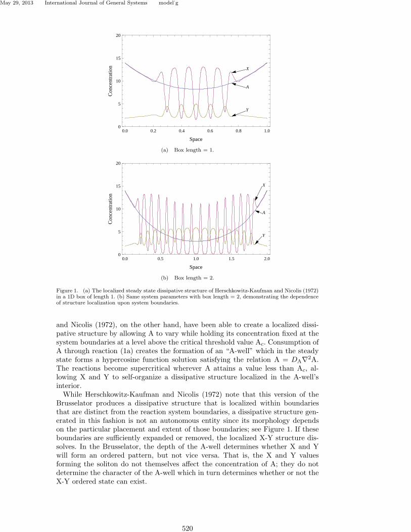
Figure 1. (a) The localized steady state dissipative structure of Herschkowitz-Kaufman and Nicolis (1972)in a 1D box of length 1. (b) Same system parameters with box length = 2, demonstrating the dependenceof structure localization upon system boundaries.

and Nicolis (1972), on the other hand, have been able to create a localized dissi-pative structure by allowing A to vary while holding its concentration fixed at thesystem boundaries at a level above the critical threshold value Ac. Consumption ofA through reaction (1a) creates the formation of an “A-well” which in the steadystate forms a hypercosine function solution satisfying the relation A = DA∇2A.The reactions become supercritical wherever A attains a value less than Ac, al-lowing X and Y to self-organize a dissipative structure localized in the A-well’sinterior.

While Herschkowitz-Kaufman and Nicolis (1972) note that this version of theBrusselator produces a dissipative structure that is localized within boundariesthat are distinct from the reaction system boundaries, a dissipative structure gen-erated in this fashion is not an autonomous entity since its morphology dependson the particular placement and extent of those boundaries; see Figure 1. If theseboundaries are sufficiently expanded or removed, the localized X-Y structure dis-solves. In the Brusselator, the depth of the A-well determines whether X and Ywill form an ordered pattern, but not vice versa. That is, the X and Y valuesforming the soliton do not themselves affect the concentration of A; they do notdetermine the character of the A-well which in turn determines whether or not theX-Y ordered state can exist.

520


-10 -5 0 5 10-0.1

0.0

0.1

0.2

0.3

0.4

0.5

0.6

0.7

Space

Con

cent

ratio

n

a

X

Y

Figure 2. Localized dissipative structure of Koga and Kuramoto (1980). DX = 1, DY = 5, a = 0.254,b = 0.5, c = 0.5.

Koga and Kuramoto (1980) simulated a localized dissipative structure supportedby a system defined by the equations:

∂X

∂t= DX∇2X−X−Y −H(X− a) (2a)

∂Y

∂t= DY∇2Y + bX− cY (2b)

where a, b, c are system constants, and H is the Heaviside step function. In thecenter of the soliton, there is a finite region in which X > a and thus H = 1, outsideof which H = 0. See Figure 2. With this mechanism the structure maintains itslocalized form. It is important to note, however, that an equation that uses theunit step H in this way is not expressible as a finite set of reaction equations(e.g. eqs. (1)) and therefore we would not classify this dissipative system as a R-Dsystem.

However, a minor variation of the Brusselator, a three-variable R-D systemknown as Model G, has been theorized in 1980 to support localized, self-stabilizingTuring patterns within a subcritical environment when the values of its systemparameters are properly chosen (LaViolette, 1985, 1994, 2008, 2010). It is able toform a true dissipative soliton, one whose structure is stable, autonomous, local-ized, and unaffected by the positions of the system boundaries. Its system of partialdifferential equations are derived from a simple set of kinetic reaction equationswith diffusion, and is in fact the earliest R-D system proposed to support solitons.Others have since reported simulation results of dissipative solitons, such as Schenket al. (1998) who investigated a two-variable system of the FitzHugh-Nagumo (FN)type. Surveys of dissipative solitons produced by dissipative systems of both theR-D and non-R-D types are given by Purwins et al. (2005), Bodeker (2007) andVanag and Epstein (2007).

Dissipative solitons have generated substantial interest because of the variety ofparticle-like properties they have been shown to produce such as scattering, reflec-tion, particle-particle bonding, orbital motion, particle annihilation, and particlereplication (Bode et al., 2002; Bodeker, 2007; Liehr et al., 2004; Nishiura et al.,2005; Purwins et al., 2005; Schenk et al., 1998; Vanag and Epstein, 2007). Previouspublications have demonstrated that Model G can form the basis for a unified fieldtheory that effectively accounts for a variety of microphysical and macrophysicalphenomena (LaViolette, 1985, 1986, 1992, 2005, 2008, 2010). In this paper, we

521


present computer simulation results carried out for the first time on this promisingreaction system.

2. Model G

Model G is a modification of the Brusselator in which a third intermediary variableG is inserted into the first reaction step (1a). It is specified by the following fivetransformations:

Ak1

k−1

G (3a)

Gk2

k−2

X (3b)

B + Xk3

k−3

Y + Z (3c)

2X + Yk4

k−4

3X (3d)

Xk5

k−5

Ω (3e)

where reaction step (1a) is replaced by the two reactions (3a, 3b). This R-D systemis represented by the following system of partial differential equations:

∂G

∂t= DG∇2G− (k−1 + k2)G + k−2X + k1A (4a)

∂X

∂t= DX∇2X + k2G− (k−2 + k3B + k5)X

+ k−3ZY − k−4X3 + k4X

2Y + k−5Ω

(4b)

∂Y

∂t= DY∇2Y + k3BX− k−3ZY + k−4X

3 − k4X2Y. (4c)

Since the forward kinetic constants have values much greater than the reversekinetic constants, the reactions have the overall tendency to proceed irreversibly tothe right. Nevertheless, the reverse reaction G← X in eq. (3b) plays an importantrole. This allows the concentration of the X variable to influence the concentrationvalue of the G variable which in turn serves as the system’s bifurcation parameter.So, because Model G’s bifurcation parameter is able to vary in both time and space,and be influenced by its X variable which participates in forming a soliton-likedissipative structure, this reaction system is able to nucleate a structure which, inthe positive Y polarity (negative X), is autonomous and self-stabilizing. All that isneeded is a momentary localized fluctuation in one of the reactants sufficiently largein amplitude and spatiotemporal breadth to initiate the growth of the soliton. Thistechnique of allowing a third reactant to serve as a variable bifurcation parameterfor the other two reactants is a recipe general enough for potential applicabilityto other dissipative-structure-producing R-D systems, allowing them to supportdissipative solitons as well.

The seed fluctuation may be in the form of an extra term that is added to theR-D equations, or it may be directly incorporated within the R-D equations by

522


representing the concentration of each reactant with a stochastic term. Such “zero-point” fluctuations would be present if each reactant is comprised of a pluralityof constituent units (e.g., X-ons, Y-ons, G-ons) which engage in Markovian birth-death transformations.

A positive polarity seed fluctuation (negative X, or positive Y), arising sponta-neously in this fashion, is able to spawn a periodic structure even when the systemis initially in a subcritical homogeneous steady state. The Brusselator, on the otherhand, must always begin from an initially supercritical homogeneous steady state.As a result, its structures are always destined to fill the entire reaction volume toits supercritical limits. This autogenic ability, wherein a stable dissipative solitoncan form spontaneously out of system noise, is an important distinctive feature ofModel G. LaViolette (1985, 2010) has shown that this feature makes Model G apromising candidate for modeling the formation of subatomic particles out of thezero-point energy continuum vacuum state. How Model G has been employed tomodel subatomic particles is further elaborated on in Section 3.1.

2.1 Nondimensionalization

In analyzing eqs. (4), we first pass to dimensionless variables. This reduces thenumber of independent system parameters by seven, significantly simplifying thegoal of finding a particular set of system parameters (eqs. (17) below) that supportthe formation of a stable soliton. In addition, this conveniently scales the dimen-sionless space, time, and concentration potential values to the order of unity in thevicinity of the soliton formation event.

We assume that the three diffusion constants DG, DX, DY, four concentrationsA, B, Z, Ω, and the ten kinetic reaction rates k±i are constant in time and space.

The dimensional space, time, and concentration variables x, y, z, t, G, X, Y areconverted to their corresponding dimensionless variables x, y, z, t,G,X, Y via thefollowing substitutions:

x = Lx, y = Ly, z = Lz, t = Tt

G(x, y, z, t) = CG(x, y, z, t) (5)

X(x, y, z, t) = CX(x, y, z, t)

Y(x, y, z, t) = CY (x, y, z, t)

where the time, space, and concentration constants are defined, respectively, as:

T ≡ 1

k−2 + k5, L ≡

√

DGT, C ≡ 1√k4T

. (6)

These substitutions allow for eqs. (4) to be expressed in terms of dimensionlessvariables:

∂G

∂t= ∇2G− qG + gX + a (7a)

∂X

∂t= dx∇2X + pG− (1 + b)X + uY − sX3 + X2Y + w (7b)

∂Y

∂t= dy∇2Y + bX − uY + sX3 −X2Y (7c)

523


where

dx ≡DX

DG, dy ≡

DY

DG,

a ≡ k1

√k4

(k−2 + k5)3/2A, b ≡ k3

k−2 + k5B, g ≡ k−2

k−2 + k5, p ≡ k2

k−2 + k5, (8)

q ≡ k−1 + k2

k−2 + k5, s ≡ k−4

k4, u ≡ k−3

k−2 + k5Z, w ≡

√k4k−5

(k−2 + k5)3/2Ω.

The vector operator ∇ is taken with respect to the dimensional x, y, z terms ineqs. (4) and with respect to the dimensionless x, y, z in eqs. (7). Since there willnever be ambiguity in its context, we use the same symbol ∇ for both.

2.2 Redimensionalization

The dimensional diffusion coefficients, kinetic constants, and constant concentra-tions A, B, Z, Ω are given as follows when expressed in terms of their dimensionlesscounterparts and T, L, C:

DG =L2

T, DX =

L2

Tdx, DY =

L2

Tdy,

k1A =C

Ta, k2 =

1

Tp, k3B =

1

Tb, k4 =

1

C2T, k5 =

1

T(1− g), (9)

k−1 =1

T(q − p), k−2 =

1

Tg, k−3Z =

1

Tu, k−4 =

1

C2Ts, k−5Ω =

C

Tw.

2.3 Homogeneous Steady State

The homogeneous steady state is one in which

0 =∂G

∂t=

∂X

∂t=

∂Y

∂t(10a)

0 = ∇G = ∇X = ∇Y. (10b)

Under these conditions the differential equations (7) become algebraic with G, X,Y having the following respective solutions:

G0 =a + gw

q − gp, X0 =

pa + qw

q − gp, Y0 =

sX20 + b

X20 + u

X0. (11)

2.4 Concentration Potentials

It proves useful to consider concentration values relative to the homogeneous steadystate (LaViolette, 1985, 1994, 2008). These concentration potentials are defined as:

ϕG ≡ G−G0, ϕX ≡ X −X0, ϕY ≡ Y − Y0. (12)

524


Eqs. (7) are expressed in terms of concentration potentials as:

∂ϕG

∂t= ∇2ϕG − qϕG + gϕX (13a)

∂ϕX

∂t= dx∇2ϕX + pϕG − (1 + b)ϕX + uϕY

− s(

(ϕX + X0)3 −X3

0

)

+(

(ϕX + X0)2(ϕY + Y0)−X2

0Y0

)

(13b)

∂ϕY

∂t= dy∇2ϕY + bϕX − uϕY

+ s(

(ϕX + X0)3 −X3

0

)

−(

(ϕX + X0)2(ϕY + Y0)−X2

0Y0

)

.

(13c)

This substitution is especially important when calculating numerical solutions forG, X, and Y that correspond to a dissipative soliton, which, as will be seen below,consists of small deviations about the homogeneous steady state values G0, X0,and Y0.

3. Particle Formation and Structure in Model G

We examine the evolution of the system in 1, 2, and 3 dimensions of space. Inthe case of 2 and 3 dimensions, circular and spherical symmetry, respectively, areimposed upon the system.1

Each concentration potential is a function of both position x in 1D (radius r inthe case of 2D and 3D) and time t. The reaction spatial domain and total time isspecified as −50 ≤ x ≤ 50 in 1D (0 ≤ r ≤ 50 in 2D and 3D) and 0 ≤ t ≤ 100.

The boundary conditions for 1D are:2

∀x ∈ [−50, 50] : ∀t ∈[0, 100] :

ϕG(x, t) ≥ −G0, ϕX(x, t) ≥ −X0, ϕY (x, t) ≥ −Y0 (14a)

ϕG(x, 0) = 0, ϕX(x, 0) = 0, ϕY (x, 0) = 0 (14b)

ϕG(±50, t) = 0, ϕX(±50, t) = 0, ϕY (±50, t) = 0. (14c)

For 2D and 3D, the boundary conditions are:

∀r ∈ [0, 50] : ∀t ∈[0, 100] :

ϕG(r, t) ≥ −G0, ϕX(r, t) ≥ −X0, ϕY (r, t) ≥ −Y0 (15a)

ϕG(r, 0) = 0, ϕX(r, 0) = 0, ϕY (r, 0) = 0 (15b)

ϕG(50, t) = 0, ϕX(50, t) = 0, ϕY (50, t) = 0 (15c)

(ϕG)r (ε, t) = 0, (ϕX)r (ε, t) = 0, (ϕY )r (ε, t) = 0. (15d)

The subscript r in eqs. (15d) denote the partial derivative with respect to r.

1The circular and spherical symmetry conditions in 2 and 3 dimensions that are imposed upon the systemare due entirely to the limited availability of computational resources for this research project at the time ofthis publication. The mathematics, as well as the simulation software, is general enough for these symmetryrestrictions to be removed—it is only a matter of acquiring sufficient computational time (CPU cycles)and space (memory) to carry out the simulations.2“∀” is the universal quantifier symbol. The first line of eqs. (14) reads “For all x between −50 and 50,and for all t from 0 to 100:”

525


Since the soliton shall be centered at the point r = 0, the boundary condition atr = 0 must not constrain the concentration potential values at this point. Instead,the boundary condition is placed upon their first order derivatives with respectto r. Under the imposed constraints of angular symmetry in 2D and 3D, thesederivatives must vanish.

Epsilon, ε, is a small positive number to numerically approximate zero. ε 6= 0for computational reasons only, due to the indeterminate form the rotationally-symmetric Laplacian takes in 2D and 3D at r = 0:

∇2ϕ =∂2ϕ

∂r2+

n− 1

r

∂ϕ

∂r(16)

where n ∈ 1, 2, 3 is the number of spatial dimensions. The point at r = 0 issmoothly approximated since the limit of ∇2ϕ as r → 0 is always finite. Thenumerical simulations in this work use ε = 10−9.

There are an infinite continuum of parameter values that allow for the creation ofa stationary soliton. The particular set of values that is investigated in this articleare the following:

dx = 1, dy = 12, a = 14, b = 29, g = 1/10,

p = 1, q = 1, s = 0, u = 0, w = 0. (17)

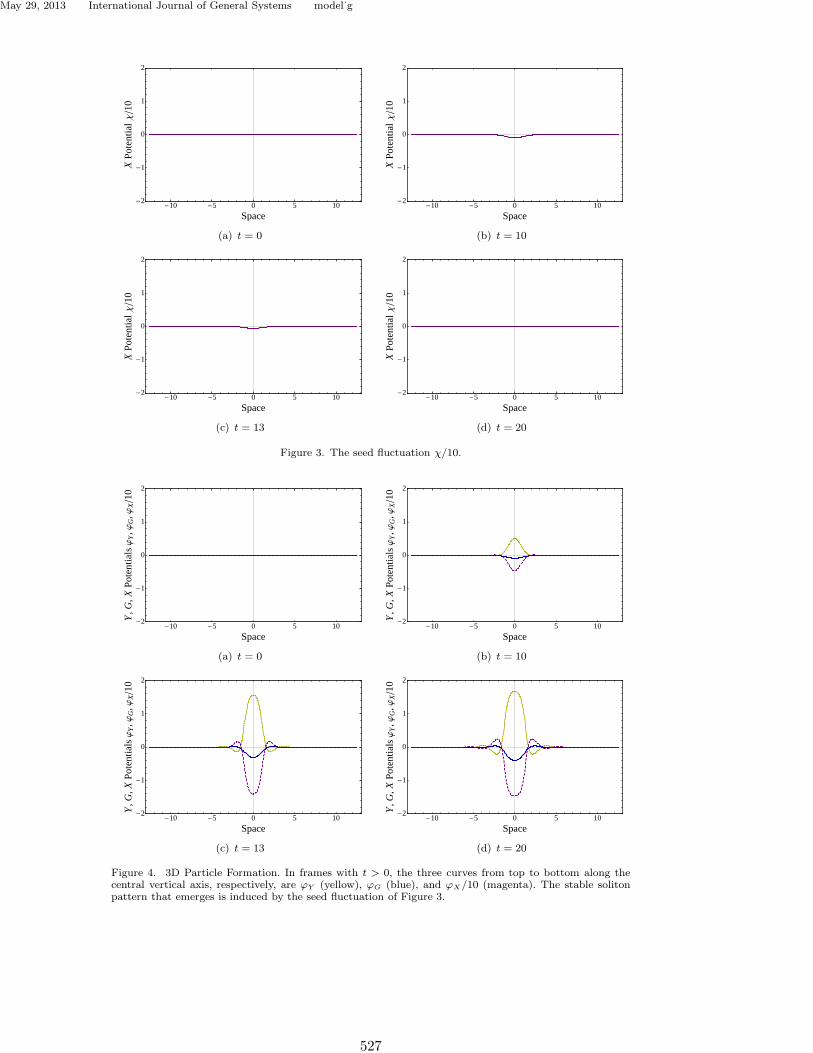
If the system is left to evolve according to eqs. (13–17), the concentrations willremain at their homogeneous steady state values, i.e. 0 = ϕG = ϕX = ϕY for all rand t. In order to initiate the formation of a soliton, we introduce a momentaryseed fluctuation in the X variable specified as χ:

χ(r, t) ≡ −e−r2

2 e−(t−10)2

18 . (18)

The time evolution of this fluctuation is graphed in Figure 3 as χ/10 for fourparticular points in time.

For one spatial dimension, r in the above equation is replaced with x. This seedfluctuation is incorporated into the system by adding χ to the right-hand side ofeq. (13b). In addition, substituting values (17) into eqs. (13), yields the followingsystem of nonlinear PDEs:

∂ϕG

∂t= ∇2ϕG − ϕG + ϕX/10 (19a)

∂ϕX

∂t= ∇2ϕX + ϕG − 30ϕX − 4060/9 + (ϕX + 140/9)2(ϕY + 261/140) + χ (19b)

∂ϕY

∂t= 12∇2ϕY + 29ϕX + 4060/9 − (ϕX + 140/9)2(ϕY + 261/140). (19c)

Eqs. (19), along with the boundary conditions (14 or 15), may then be numericallysolved on a computer.

3.1 Particle Structure in 3D

Figure 4 shows the computer-simulated evolution of ϕG, ϕX , and ϕY under eqs. (19)in three spatial dimensions, subject to boundary conditions (15) and graphed attimes t = 0, t = 10, t = 13 and t = 20.

526


-10 -5 0 5 10-2

-1

0

1

2

Space

XPo

tent

ialΧ1

0

(a) t = 0

-10 -5 0 5 10-2

-1

0

1

2

Space

XPo

tent

ialΧ1

0

(b) t = 10

-10 -5 0 5 10-2

-1

0

1

2

Space

XPo

tent

ialΧ1

0

(c) t = 13

-10 -5 0 5 10-2

-1

0

1

2

Space

XPo

tent

ialΧ1

0

(d) t = 20

Figure 3. The seed fluctuation χ/10.

-10 -5 0 5 10-2

-1

0

1

2

Space

Y,G

,XPo

tent

ialsj

Y,j

G,j

X1

0

(a) t = 0

-10 -5 0 5 10-2

-1

0

1

2

Space

Y,G

,XPo

tent

ialsj

Y,j

G,j

X1

0

(b) t = 10

-10 -5 0 5 10-2

-1

0

1

2

Space

Y,G

,XPo

tent

ialsj

Y,j

G,j

X1

0

(c) t = 13

-10 -5 0 5 10-2

-1

0

1

2

Space

Y,G

,XPo

tent

ialsj

Y,j

G,j

X1

0

(d) t = 20

Figure 4. 3D Particle Formation. In frames with t > 0, the three curves from top to bottom along thecentral vertical axis, respectively, are ϕY (yellow), ϕG (blue), and ϕX/10 (magenta). The stable solitonpattern that emerges is induced by the seed fluctuation of Figure 3.

527


Y,G

and

XPo

tent

ials

-10 -5 0 5 10-2

-1

0

1

2

jY

jG

jX

10

Space

(a) Spherically-symmetric 3D stationary particle.

Y,G

and

XPo

tent

ials

-10 -5 0 5 10-0.02

-0.01

0.00

0.01

0.02

jY

jG

jX

10

Space

(b) Zoomed 100×.

Figure 5. (a) Spherically-symmetric 3D stationary particle formed from eqs. (19) and boundary condi-tions (15). (b) Same data zoomed 100× vertically.

The system converges to the stationary structure shown in Figure 5(a). Thisstable soliton is what is identified in Model G as an individual particle. Thesesimulation results show that the reaction variables produce a periodic pattern ofprecise wavelength, λ0 = 3.08 units, that progressively decreases in amplitude asit extends outward from a central bell-shaped core. Figure 5(b) exhibits the extentof the periodicity of the particle’s potential fields by zooming the vertical axis ofthe simulation 100×.

The subquantum kinetics physics methodology developed by LaViolette (1985,2008, 2010, 2012) postulates that subatomic particles are electric and gravity po-tential solitons. It identifies the ϕG variable with gravity potential and the ϕX andϕY variables with electric potential. Negative ϕG values are associated with pos-itive, matter-attracting gravitational mass and positive ϕG values are associatedwith negative, matter-repelling gravitational mass. Positive and negative ϕY values(negative and positive ϕX values) are associated respectively with positive and neg-ative charge, the ϕX and ϕY variables having a reciprocal relation to one another.Since the ϕG and ϕX potentials are closely coupled in Model G due to the linkage ofspecies G and X through both forward and reverse reactions, subquantum kineticspredicts that the electric and gravitational potentials should be closely coupled:negative gravity potential with positive electric potential. Thus in subquantum ki-netics, subatomic particles are envisioned as local field potential inhomogeneities.

528


Since these particular inhomogeneities share a common Turing wave pattern mor-phology, this leads to a natural quantization of these fields into identical particles.This is reminiscent of the quantization of fermionic matter fields in quantum fieldtheory which is invoked to explain why those fields’ particles are identical.

The simulation displayed in Figures 4 and 5 would be interpreted in subquantumkinetics as the nucleation of a neutral subatomic particle, a neutron for example,being nucleated by a positive charge polarity electric potential fluctuation emergingfrom the subquantum zero-point energy field. In this case the particle’s core has apositive electric potential coinciding with a negative gravity potential and creatinga local stabilizing supercritical domain. In subquantum kinetics, such fluctuationscan trigger particle nucleation even though they themselves have a field energypotential magnitude much smaller than that of the particle they nucleate. A neg-atively charged fluctuation would lead to the formation of an antimatter particlehaving a core with a negative electric potential coinciding with a positive gravitypotential. But, as LaViolette (1985) has pointed out, such negative charge polar-ity fluctuations emerging from system noise where the reaction system is initiallysubcritical, as would be the case for the primordial vacuum state, fail to nucleatea particle. He notes that Model G’s ability to nucleate solitons with an inherentpolarity bias favoring the matter state is a feature that is advantageous in the ap-plication to cosmology where nature has favored the primordial creation of matterover antimatter.

These modeling results confirm LaViolette’s 1985 prediction that Model G shouldgenerate a dissipative space structure whose field potential has this same form: agaussian core surrounded by an extended asymptotic field periodicity. He proposedthat such a field potential could serve as a useful model of a subatomic particleprovided that the reaction system parameters are chosen such that the wavelengthof the soliton’s oscillatory tail equals the subatomic particle’s Compton wavelength.He demonstrated that this periodic tail, which he termed the particle’s Turing

wave, accounts for the experimental results of both particle diffraction and orbitalquantization (LaViolette, 1985, 1994, 2010).

Later, LaViolette (2008, 2010) noted that the ϕY (and ϕX) wave pattern predictedfor Model G’s Turing wave soliton field pattern has a morphology very similar tothe charge distribution model that Kelly (2002) derived for the core of the nucleonby analyzing form factor data obtained from high energy electron beam particlescattering experiments. Kelly obtained a best fit to this scattering data by assumingthat the nucleon’s charge and magnetization distribution had the form of a gaussiancore surrounded by a periodicity having a wavelength approximating the nucleon’sCompton wavelength. The simulation results presented here further support thissuggestion in that they indicate that the ϕX and ϕY field pattern generated byModel G displays morphological features similar to those of the radial electriccharge distribution in the neutron and proton and should therefore serve as anappropriate soliton field structure for modeling subatomic particles.

The amplitude of the ϕX (or ϕY ) field maxima forming the simulated Model Gsoliton are observed to decline as r−3.7 at r ≈ 2λ0, as r−7 at r ≈ 4λ0, and as r−10

at r ≈ 6λ0. This may be compared with r−7 in standard theories for the radialdecline of the nuclear force. Because of this rapid decline, the product of the Turingpattern field amplitude with incremental shell volume diminishes toward zero forshells of successively greater radius, and the sum of these shell product incrementsconverges to a finite value. A finite value for the soliton negentropy makes Model Gattractive as a model of a subatomic particle since subquantum kinetics identifiesthe ϕX , ϕY field magnitudes forming the Model G soliton, with both the electricfield forming the particle’s core and with the particle’s inertial mass (LaViolette,

529


Bou

ndar

yR

adiu

s

0 5 10 15 20 2522

23

24

25

26

27

Particle Radius r

(a) Zeroes of ϕX with a variable system boundary.

Zer

opoi

ntSp

acin

g

æ

æ

æ

ææ æ æ æ æ æ æ æ æ æ æ æ æ æ æ æ æ æ æ æ æ æ æ æ æ

æ

æ

æ

à

à

à

à

à

à

à

àà à à à à à à à à à à à à à à à à à à à à

à

à

à

ì

ì

ì

ììì ì ì ì ì ì ì ì ì ì ì ì ì ì ì ì ì ì ì ì ì ì ì ì

ì

ì

ì

0 10 20 30 40 501.2

1.3

1.4

1.5

1.6

1.7

1.8

1.9

æ jY

à jG

ì jX

Midpoint Between Zeropoints

(b) Differences and locations of zeroes for ϕY , ϕG, and ϕX .

Figure 6. The Turing wavelength is independent of the distance between the particle core and systemboundary, and is the same value for each reactant. Figure (a) shows the periodic locations of the zeroesof ϕX (horizontal axis) for a spherically-symmetric 3D particle centered at r = 0, with a variable systemradius (vertical axis), demonstrating that the Turing wavelength is independent of the size of the enclosingsystem volume. Figure (b) shows the successive differences between zeroes for ϕY , ϕG, and ϕX (verticalaxis) for a 1D particle at the midpoints between each zero-pair (horizontal axis). The central alignmentof zero differences demonstrates that the Turing wavelength is the same for each reactant, equal to 3.08(twice the distance between zeroes). Similar results were found for circularly and spherically symmetric2D and 3D particles, respectively.

1985, 2010).We also report the simulation results of producing ordered patterns with Model

G where the reaction vessel size was progressively increased. The Turing patternperiodicity was found to persist to the vessel boundaries and to maintain a constantwavelength as the vessel size was expanded. This is shown in Figure 6(a) whichplots the radial distance locations of the ϕX zero values (horizontal axis) againstthe radial size of the spherical reaction volume (vertical axis), and shows how theparticle’s fields adjust in the vicinity of the steady-state boundary conditions. Thepersistence of this wave pattern and invariance of its wavelength with increasingvessel size demonstrates that the Turing pattern is independent of the boundaryconditions. These results also confirm the predictions of LaViolette (1994, 2008)that the Model G Turing pattern should persist outward to large radial distances inorder to properly model the particle diffraction phenomenon. The pattern, though,would have the inherent radial limit at the radial distance where the noise ampli-tude present in the stochastic variation of each reactant concentration exceeds theTuring wave pattern amplitude.

530


3.2 Comparison of Particle Structures Simulated in 1D, 2D, and 3D

When Model G is simulated in 1D and 2D, it produces particles whose cores arenarrower and lower in amplitude, although their Turing wavelength remains thesame. Figure 7 shows the 1D and 2D particles formed from eqs. (19) and boundaryconditions (14) and (15), respectively. Compare these to Figure 5(a). Specific valuesof the structural characteristics of the 1D, 2D, and 3D particles are shown inTable 1. The core radius, Table 1, row (b), is defined as the inner-most zero-pointfield potential crossing r0 (the least positive value for which ϕ(r0) = 0) for eachof the concentration potentials). Note that the radius in all cases is largest forϕG and smallest for ϕX . The core RMS radius, the root mean square radius rRMS

listed in row (c), for each concentration potential in each of the three dimensionsis calculated as:

rRMS =√

〈r2〉

=

√

∫

S ϕ(r)r2dS∫

S ϕ(r)dS.

(20)

The integral in the denominator of the above formula is the core integral, row (d),which is given by:

∫

Sϕ(r)dS =

∫ r0

−r0

ϕ(r)dr in 1D,

2π

∫ r0

0ϕ(r)rdr in 2D,

4π

∫ r0

0ϕ(r)r2dr in 3D

(21)

where the domain of integration S is the space within the core radius r0 definedby each of the concentration potentials. The full integral values, row (e), use thesame formulas as the core integral, but with r0 going out to the system boundary.

The Turing wavelength, row (f), is found by first calculating successive differencesbetween the zeroes of each of the 3 concentration potentials ϕY , ϕG, ϕX . Figure 6(b)illustrates that this is a well-defined value for all 3 concentrations at a sufficientdistance away from both the particle’s central core and the system boundaries.The mean is calculated from the centrally-aligned data points and doubled (thedistance between zeroes is a half-wavelength) resulting in a value of 3.08. This sameλ0 value to 3 significant figures was found in dimensions 1D, 2D, and 3D, wherecircular and spherical symmetry was imposed in the 2D and 3D cases, respectively.

4. Particle Physics in Model G

The solitons of Model G exhibit a number of properties resembling those commonlyassociated with subatomic particles. Earlier we noted that the morphology of theModel G solitons, their bell-shaped core surrounded by a Turing wave pattern ofprecise wavelength, has been found to be a good description of the core field of anucleon. Another advantage mentioned earlier is that the full integral of the fieldpotential converges to a finite value. Other characteristics discussed here includeparticle-particle bonding (i.e., equivalent to nuclear bonding), the gravitational

531


Y,G

and

XPo

tent

ials

-10 -5 0 5 10-1.0

-0.5

0.0

0.5

1.0

jY

jG

jX

10

Space

(a) 1D stationary particle.

Y,G

and

XPo

tent

ials

-10 -5 0 5 10

-1.5

-1.0

-0.5

0.0

0.5

1.0

1.5

jY

jG

jX

10

Space

(b) Circularly-symmetric 2D stationary particle.

Figure 7. (a) 1D and (b) 2D stationary particles formed from eqs. (19) and boundary conditions (14, 15).

mass polarity in a particle with spin, and particle movement in a gravitationalgradient.

4.1 Multi-particle States in 1D

The single particle discussed in Section 3 was seeded from a single gaussian fluctu-ation χ defined in eq. (18). In a similar way, multiple particles may be seeded frommultiple gaussian fluctuations, and when seed fluctuations are spaced sufficientlyclose together, the resulting particles are able to coexist with one another at spe-cific distances of separation. We examined cases in which particles are seeded in1D from two and three gaussian seed fluctuations.

To seed two proximal particles, we define the double-gaussian seed fluctuation:

χ2(x, t) ≡ χ(x + d2/2, t) + χ(x− d2/2, t) (22a)

d2 = 3.303 (22b)

and replace χ with χ2 in eqs. (19) under boundary conditions (14). Figure 8(a)shows the stationary two-particle solution that the system converges to by t = 100.The final distance between the particles, defined as the distance between the coreextrema of ϕX , is found to be 3.303, or about one Turing wavelength. This finalparticle distance is converged to even when d2 in eq. (22a) is varied by small

532


Table 1. Particle structure values in dimensionless units.

1D 2D 3D 2Dδ

(a) Core amplitudeϕY 0.930 1.50 1.70 1.53ϕG -0.161 -0.308 -0.411 -0.320ϕX -8.36 -13.6 -14.6 -13.8

(b)Core radius(first zero)

ϕY 0.724 1.21 1.68 1.67ϕG 0.867 1.37 1.85 1.87ϕX 0.642 1.13 1.61 1.58

(c) Core RMS radiusϕY 0.302 0.665 1.07 0.929ϕG 0.363 0.739 1.14 1.02ϕX 0.272 0.634 1.04 0.892

(d) Core integralϕY 0.806 3.12 13.2 6.31ϕG −0.167 −0.710 −3.17 −1.44ϕX −6.59 −26.3 −111 −53.6

(e) Full integralϕY 0.281 0.893 3.30 2.96ϕG 8.39× 10−5 2.88 × 10−3 2.87 × 10−2 −0.480ϕX 6.01× 10−4 0.128 1.93 −13.7

(f) Turing wavelength 3.08 3.08 3.08 3.08

amounts both higher and lower. For example when d2 = 4, the same 3.303 distancebetween the particles is converged to. For this reason we may conclude that theparticles coexist in a bonded relationship to one another.

To seed three proximal particles, we define the triple-gaussian seed fluctuation:

χ3(x, t) ≡ χ(x + d3, t) + χ(x, t) + χ(x− d3, t) (23a)

d3 = 3.314. (23b)

Figure 8(b) shows the stationary three-particle solution the system converges toby t = 100. The final distance between the particles is 3.314, which again is astable value that is converged to even when we make small variations in d3. Futurework will determine if such particle bonding also occurs in 2D and 3D simulations ofModel G. Others working with the FN and FN-type models, who have simulated 2Ddissipative solitons with oscillatory tails, also report particle-particle bonding andthe formation of aggregate structures variously termed “clusters” or “molecules”,although these are formed when the solitons have initial velocities relative to oneanother (Bode et al., 2002; Purwins et al., 2005; Schenk et al., 1998). As is the casewith the 1D simulations of Model G, these bound FN solitons are similarly foundto align their concentration peaks with those of their partner.

When a two-particle simulation is performed with d2 = 6.628, the two fluctu-ations being separated by the same distance as between the outer two particlesof the three-particle stable state, two particles are initially created from the χ2

seed fluctuations. However, the G potential well and Y potential hill formed inthe space between them by the overlapping soliton tails provide a fertile environ-ment that allows the spontaneous emergence of a third particle. This three-particle

533


Y,G

and

XPo

tent

ials

-10 -5 0 5 10

-1.0

-0.5

0.0

0.5

1.0

jY

jG

jX

10

Space

(a) Two 1D stationary bonded particles.

Y,G

and

XPo

tent

ials

-10 -5 0 5 10

-1.0

-0.5

0.0

0.5

1.0

jY

jG

jX

10

Space

(b) Three 1D stationary bonded particles.

Figure 8. (a) Two and (b) three 1D stationary particles formed from eqs. (19) and boundary condi-tions (14), where χ is replaced by (a) χ2 and (b) χ3.

state then converges to the same three-particle state depicted in Figure 8(b). Thisconfirms the earlier expectation that in Model G existing particles should producefavorable conditions facilitating additional particle autogenesis (LaViolette, 1985,1994, 2010). Again, further work is needed to determine if mother-daughter particlecreation also takes place in 2D and 3D simulations of Model G.

Two dimensional simulations of the FN model carried out by other researchershave also demonstrated the dissipative soliton particle replication phenomenon(Bodeker, 2007; Liehr et al., 2003; Purwins et al., 2005). In one case four parti-cles move towards one another, collide, and form a stable bound cluster. Then afifth soliton nucleates at the cluster’s geometrical center where the concentrationmaxima of their innermost shells intersect and thereby produce a combined concen-tration maximum that is sufficiently great to induce spontaneous generation of thefifth particle. So this replication process occurs in the FN model in much the samefashion, although Model G spawns its progeny particles from initially stationaryparent particles.

4.2 Particle “Mass”

Looking at Figure 5(a), it may appear as if the full integral of ϕG should be negative,due to the large central G-well, compared to the smaller G-hills that surround it.However, the contribution from these surrounding G-hill shells ultimately outweigh

534


Y,G

and

XPo

tent

ials

-10 -5 0 5 10

-1.5

-1.0

-0.5

0.0

0.5

1.0

1.5

jY

jG

jX

10

Space

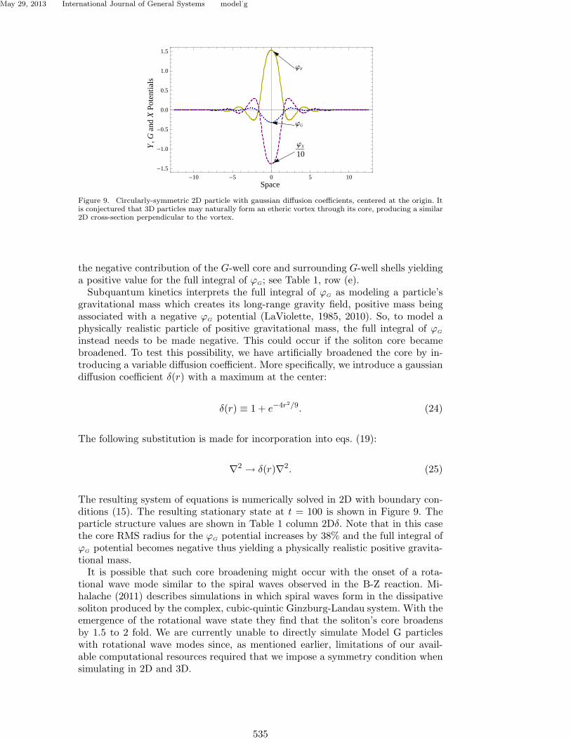
Figure 9. Circularly-symmetric 2D particle with gaussian diffusion coefficients, centered at the origin. Itis conjectured that 3D particles may naturally form an etheric vortex through its core, producing a similar2D cross-section perpendicular to the vortex.

the negative contribution of the G-well core and surrounding G-well shells yieldinga positive value for the full integral of ϕG; see Table 1, row (e).

Subquantum kinetics interprets the full integral of ϕG as modeling a particle’sgravitational mass which creates its long-range gravity field, positive mass beingassociated with a negative ϕG potential (LaViolette, 1985, 2010). So, to model aphysically realistic particle of positive gravitational mass, the full integral of ϕG

instead needs to be made negative. This could occur if the soliton core becamebroadened. To test this possibility, we have artificially broadened the core by in-troducing a variable diffusion coefficient. More specifically, we introduce a gaussiandiffusion coefficient δ(r) with a maximum at the center:

δ(r) ≡ 1 + e−4r2/9. (24)

The following substitution is made for incorporation into eqs. (19):

∇2 → δ(r)∇2. (25)

The resulting system of equations is numerically solved in 2D with boundary con-ditions (15). The resulting stationary state at t = 100 is shown in Figure 9. Theparticle structure values are shown in Table 1 column 2Dδ. Note that in this casethe core RMS radius for the ϕG potential increases by 38% and the full integral ofϕG potential becomes negative thus yielding a physically realistic positive gravita-tional mass.

It is possible that such core broadening might occur with the onset of a rota-tional wave mode similar to the spiral waves observed in the B-Z reaction. Mi-halache (2011) describes simulations in which spiral waves form in the dissipativesoliton produced by the complex, cubic-quintic Ginzburg-Landau system. With theemergence of the rotational wave state they find that the soliton’s core broadensby 1.5 to 2 fold. We are currently unable to directly simulate Model G particleswith rotational wave modes since, as mentioned earlier, limitations of our avail-able computational resources required that we impose a symmetry condition whensimulating in 2D and 3D.

535


4.3 1D Particle Movement in a Gravitational Gradient

The movement of a 1D particle is examined in the presence of a G-gradient. TheG-gradient of slope m is incorporated into the system by adding the function

γm(x, t) =

0 if t < 100,

mx + 10−4/6 if 100 ≤ t(26)

to the right-hand side of eq. (13a). This function allows the particle to form fromt = 0 to 100, then “turns on” a G-gradient of slope m from t = 100 to 200, duringwhich time we examine the particle’s positions and velocities.

Using the parameter substitutions again of eqs. (17) and solving the resultingsystem of PDEs under the boundary conditions

∀x ∈ [−50, 50] : ∀t ∈ [0, 200] :

α = 3875/4096 (27a)

ϕG(x, 0) = −0.161αe−1

2 (x

0.363 )2

(27b)

ϕX(x, 0) = −8.37αe−1

2(x

0.272 )2

(27c)

ϕY (x, 0) = 0.930αe−1

2(x

0.302 )2

(27d)

ϕG(±50, t) = γm(±50, t) (27e)

ϕX(±50, t) = 0 (27f)

ϕY (±50, t) = 0 (27g)

yields the same single-particle state of Figure 7(a) as done previously. The differencehere is that the particle grows from gaussian initial conditions eqs. (27b, 27c, 27d)1

rather than the seed fluctuation χ. The purpose of using these initial conditions isthat eqs. (27) produce the particle more quickly than χ does. If we were insteadto use the χ fluctuation, the 1D particle would still be “settling down” at t = 100with its core zeroes still moving on the order of 10−6 per unit time. This is theapproximate magnitude of the particle velocities due to the induced G-gradients.In contrast, the 1D particle created from these alternate initial conditions has itscore zeroes effectively stationary at this order of magnitude, allowing us to measurethe particle’s velocity in isolation of this settling effect.

The 11 values for the G-gradients m that are examined are m = −10−5k/3 fork ∈ 0, 1, 2, ..., 10. See Figures 10. The position of the particle is defined to be themidpoint between the two center-most zeroes of ϕX flanking its central minimum.This was found to be a more precise method of determining the particle’s positionthan simply calculating the location of the central minimum of ϕX , due to the factthat ϕX(x, t) is a numerical solution to the PDEs in this present analysis, and anyspecific value is numerically interpolated. Thus points along highly sloping areas ofϕX , such as its zeroes, are more accurately interpolated than local extrema, whoseprecise locations must generally be extrapolated. The initial hills in Figure 10(b)are an artifact of this method of determining the particle’s position, as the formof the particle is slightly altered by the applied G-gradient. Because of this, the

1Note the use of the Core amplitude and Core RMS radius values from Table 1 in these 3 equations. Theconstant α is an overall factor used to select initial conditions that create the particle in as little time t aspossible.

536


Part

icle

Posi

tionH´

10-

5L

100 120 140 160 180 200

0

5

10

15

20

Time

(a) 1D particle positions in 11 different G-gradients.

Part

icle

Vel

ocityH´

10-

7L

100 120 140 160 180 200

0

5

10

15

20

Time

(b) 1D particle velocities in 11 different G-gradients.

Figure 10. Positions (a) and velocities (b) of the 1D particle from t = 100 to 200 for 11 different valuesof the G-gradient m = −10−5k/3 for k = 0, 1, 2, ...,10, corresponding to the data sets displayed frombottom–up, respectively. After the G-gradient is turned on at t = 100, the particle velocity converges to aconstant value, proportional to the applied G-gradient m.

Part

icle

Vel

ocityH´

10-

6L

0 5 10 15 20 25 30

0.0

0.5

1.0

1.5

2.0

y = 0.0599x

Applied Negative G Potential Gradient H´10-6L

Figure 11. The 1D particle’s constant velocities vs. the 11 values of the applied G-gradient m form alinear relationship.

537


average of the velocities from t = 150 to 200 are used in the particle velocity vs.G-gradient plot shown in Figure 11. The 11 velocities v were found to be directlyproportional to the applied G-gradient m:

v = −0.0599m. (28)

To realistically represent microphysical phenomena, Model G would need to spawnsolitons that accelerate in a G-gradient field rather than move at a constant ve-locity. There are many aspects of Model G that still remain unexplored and wefeel that future work will demonstrate particle acceleration. In particular, future3D simulations of Model G will investigate whether 3D solitons incorporating ro-tational wave modes will be found to accelerate in G-gradients.

5. Conclusion

Features of Model G’s solitons in one, two, and three dimensions of space wereexamined, and found to have characteristics resembling those observed for sub-atomic particles. These include a structure matching observations of the nucleon’sstationary wave charge distribution, multi-particle bonding, and movement in fieldgradients. Model G was derived from the Brusselator R-D system using a recipegeneral enough to potentially generate new soliton-supporting systems from R-Dsystems that are unable to. All such systems would be interesting candidates tostudy in the context of the subquantum kinetics methodology.

Acknowledgments

MP would like to thank Kerry Cassidy and Bill Ryan of Project Camelot for theirinterview of Paul LaViolette in July of 2009.

Appendix A. Brusselator Solitons

Here we describe one other way of modifying the Brusselator in order for it tosupport dissipative solitons. This involves keeping the reaction system with justfour reactions, as it was originally specified, but allowing A to vary in addition toX and Y, and allowing non-zero reverse reaction rates for A← X and X← E. Webegin with the reversible Brusselator, which is specified by the following kineticreactions (Nicolis and Prigogine, 1977):

Ak1

k−1

X (A1a)

B + Xk2

k−2

Y + D (A1b)

2X + Yk3

k−3

3X (A1c)

Xk4

k−4

E. (A1d)

538


Expressed as PDEs with diffusion:

∂A

∂t= DA∇2A− k1A + k−1X (A2a)

∂X

∂t= DX∇2X + k1A + k−4E + k−2DY

− (k−1 + k2B + k4)X + k3X2Y − k−3X

3

(A2b)

∂Y

∂t= DY∇2Y − k−2DY + k2BX− k3X

2Y + k−3X3. (A2c)

Passing to a dimensionless system, the units of time, space, and concentrationare identified, respectively, as:

T ≡ 1

k−1 + k4, L ≡

√

DAT, C ≡ 1√k3T

. (A3)

These are used to replace the dimensional parameters with their dimensionlesscounterparts, as done in eqs. (5). Together with the dimensionless parameter sub-stitutions

dx ≡DX

DA, dy ≡

DY

DA, b ≡ k2

k−1 + k4B, g ≡ k−1

k−1 + k4, (A4)

p ≡ k1

k−1 + k4, s ≡ k−3

k3, u ≡ k−2

k−1 + k4D, w ≡

√k3k−4

(k−1 + k4)3/2E

eqs. (A2) become

∂A

∂t= ∇2A− pA + gX (A5a)

∂X

∂t= dx∇2X + pA + w + uY − (1 + b)X + X2Y − sX3 (A5b)

∂Y

∂t= dy∇2Y − uY + bX −X2Y + sX3. (A5c)

We again use the same vector operator ∇ in both equation sets (A2,A5) with theunderstanding that the prior is taken with respect to dimensional units, and thelatter dimensionless.

The homogeneous steady state values for A, X, and Y are, respectively,

A0 =gw

p(1− g), X0 =

w

1− g, Y0 =

sX20 + b

X20 + u

X0. (A6)

Defining the concentration potentials

ϕA ≡ A−A0, ϕX ≡ X −X0, ϕY ≡ Y − Y0 (A7)

and additional system constants

c0 ≡ X20 + u, c1 ≡ b− 2X0Y0 + 3sX2

0 ,

c2 ≡ 2X0, c3 ≡ Y0 − 3sX0 (A8)

539


yields

∂ϕA

∂t= ∇2ϕA − pϕA + gϕX (A9a)

∂ϕX

∂t= dx∇2ϕX + pϕA − ϕX + c0ϕY

+ (c2ϕY − c1 + (ϕY + c3 − sϕX)ϕX)ϕX

(A9b)

∂ϕY

∂t= dy∇2ϕY − c0ϕY

− (c2ϕY − c1 + (ϕY + c3 − sϕX)ϕX)ϕX .

(A9c)

Solving this system in 1D with boundary conditions

∀x ∈ [−50, 50] : ∀t ∈ [0, 100] :

ϕA(x, 0) = −0.161e−1

2(x

0.363 )2

ϕX(x, 0) = −8.37e−1

2(x

0.272 )2

ϕY (x, 0) = 0.930e−1

2 (x

0.302 )2

(A10)

ϕA(±50, t) = 0

ϕX(±50, t) = 0

ϕY (±50, t) = 0

and dimensionless parameter values

dx = 1, dy = 12, b = 29, g = 1/10,

p = 1, s = 0, u = 0, w = 14 (A11)

at t = 100 yields the same soliton configuration shown in Figure 7(a), with ϕG re-placed by ϕA. Throughout the reaction, all concentrations maintain a non-negativevalue, equivalent to the conditions ϕA ≥ −A0, ϕX ≥ −X0, and ϕY ≥ −Y0.

The same 2D and 3D soliton configurations are found as with Model G, whencircular and spherical symmetry are imposed, and with the following modifications:

• The 3 gaussian initial conditions in eqs. (A10) have their heights and widths,which are the values from rows (a) and (c) from Table 1, modified using thecorresponding 2D or 3D column.

• The Dirichlet boundary conditions at x = −50 for 1D are replaced by theNeumann boundary conditions at r = 0 for 2D and 3D, as done in equationsets (14,15).

References

Bode, M., Liehr, A., Schenk, C. and Purwins, H.G., 2002. Interaction of dissipa-tive solitons: particle-like behaviour of localized structures in a three-componentreaction-diffusion system. Physica D: Nonlinear Phenomena, 161 (1–2), 45–66.

Bodeker, H.U., 2007. Universal Properties of Self-Organized Localized Structures.Thesis (PhD). Universitat Munster.

540


Herschkowitz-Kaufman, M. and Nicolis, G., 1972. Localized Spatial Structures andNonlinear Chemical Waves in Dissipative Systems. J. of Chemical Physics, 56(5), 1890–1896.

Kelly, J.J., 2002. Nucleon Charge and Magnetization Densities from Sachs FormFactors. Physical Review C, 66 (6), 065203.

Koga, S. and Kuramoto, Y., 1980. Localized Patterns in Reaction-Diffusion Sys-tems. Progress of Theoretical Physics, 63 (1), 106–121.

LaViolette, P.A., 1985. An Introduction To Subquantum Kinetics: Parts I, II, III.Intern. J. of General Systems, 11 (4), 281–345.

LaViolette, P.A., 1986. Is The Universe Really Expanding? Astrophysical J., 301,544–553.

LaViolette, P.A., 1992. The Planetary-Stellar Mass-Luminosity Relation: PossibleEvidence of Energy Nonconservation? Physics Essays, 5 (4), 536–544.

LaViolette, P.A., 1994. Subquantum Kinetics: The Alchemy of Creation. 1st ed.Alexandria, VA: Starlane Publications (out of print).

LaViolette, P.A., 2005. The Pioneer Maser Signal Anomaly: Possible Confirmationof Spontaneous Photon Blueshifting. Physics Essays, 18 (2), 150–163.

LaViolette, P.A., 2008. The Electric Charge and Magnetisation Distribution of TheNucleon: Evidence of A Subatomic Turing Wave Pattern. Intern. J. of General

Systems, 37 (6), 649–676.LaViolette, P.A., 2010. Subquantum Kinetics: A Systems Approach to Physics and

Astronomy. 3rd ed. Niskayuna, NY: Starlane Publications.LaViolette, P.A., 2012. Subquantum Kinetics: A Systems Approach to Physics and

Astronomy. 4th ebook ed. Niskayuna, NY: Starlane Publications.Lefever, R., 1968. Dissipative Structures in Chemical Systems. J. of Chemical

Physics, 49 (11), 4977–4978.Liehr, A.W., et al., 2003. Replication of Dissipative Solitons by Many-Particle

Interaction. In: High Performance Computing in Science and Engineering ’02.,48–61 Berlin: Springer.

Liehr, A., et al., 2004. Rotating bound states of dissipative solitons in systemsof reaction-diffusion type. The European Physical J. B: Condensed Matter and

Complex Systems, 37, 199–204.Mihalache, D., 2011. Spiral solitons in two-dimensional complex cubic-quintic

Ginzburg-Landau models. Romanian Reports in Physics, 63 (2), 325–338.Nicolis, G. and Prigogine, I., 1977. Self-Organization in Nonequilibrium Systems:

From Dissipative Structures to Order Through Fluctuations. New York: JohnWiley & Sons.

Nishiura, Y., Teramoto, T. and Ueda, K.I., 2005. Scattering of traveling spots indissipative systems. Chaos, 15 (4), 047509.

Purwins, H.G., Bodeker, H. and Liehr, A., 2005. Dissipative Solitons in Reaction-Diffusion Systems. Lecture Notes in Physics, 661, 267–308.

Schenk, C.P., Schutz, P., Bode, M. and Purwins, H.G., 1998. Interaction of self-organized quasiparticles in a two-dimensional reaction-diffusion system: The for-mation of molecules. Physical Review E, 57, 6480–6486.

Turing, A.M., 1952. The Chemical Basis of Morphogenesis. Philosophical Trans. of

the Royal Society of London B: Biological Sciences, 237 (641), 37–72.Vanag, V.K. and Epstein, I.R., 2007. Localized Patterns in Reaction-Diffusion Sys-

tems. Chaos, 17 (3), 037110.Winfree, A.T., 1974. Rotating Chemical Reactions. Scientific American, 230, 82–

95.Zaikin, A.N. and Zhabotinsky, A.M., 1970. Concentration Wave Propagation in

Two-dimensional Liquid-phase Self-oscillating System. Nature, 225, 535–537.

541

stationary dissipative solitons of model g - blue science · may 29, 2013 international journal of...

Documents