static equilibria of rigid bodies: dice, pebbles, and the
TRANSCRIPT

DOI: 10.1007/s00332-005-0691-8J. Nonlinear Sci. Vol. 16: pp. 255–281 (2006)
© 2006 Springer Science+Business Media, Inc.
Static Equilibria of Rigid Bodies: Dice, Pebbles,and the Poincare-Hopf Theorem
P. L. Varkonyi and G. DomokosBudapest University of Technology and Economics, Department of Mechanics, Materials andStructures, H-1111 Muegyetem rkp. 1-3, Budapest, HungaryandCenter for Applied Mathematics and Computational Physics, Budapest, [email protected]@bagira.iit.bme.hu
Received February 1 , 2005; revised manuscript accepted for publication January 23, 2006Online publication May 22, 2006Communicated by J. E. Marsden
Summary. By appealing to the Poincare-Hopf Theorem on topological invariants, weintroduce a global classification scheme for homogeneous, convex bodies based on thenumber and type of their equilibria. We show that beyond trivially empty classes all otherclasses are non-empty in the case of three-dimensional bodies; in particular we provethe existence of a body with just one stable and one unstable equilibrium. In the caseof two-dimensional bodies the situation is radically different: the class with one stableand one unstable equilibrium is empty (Domokos, Papadopoulos, Ruina, J. Elasticity 36[1994], 59–66). We also show that the latter result is equivalent to the classical Four-Vertex Theorem in differential geometry. We illustrate the introduced equivalence classesby various types of dice and statistical experimental results concerning pebbles on theseacoast.
Key words. Static equilibria, rigid bodies, monostatic bodies, pebble shapes.
MSC numbers. 74G55, 37J05.
1. Introduction
In this paper we study the number and type of static equilibria of homogeneous, convexbodies resting on a horizontal surface without friction in the presence of uniform gravity.
Static equilibria of rigid bodies have been always present in human thought. In par-ticular, the number of stable equilibria played a key role: Archimedes provided the first
256 P. L. Varkonyi and G. Domokos
rigorous method to construct ships with one stable equilibrium [7]. Throwing dice (aswell as making decisions in gambling) relies essentially on the existence of several stableequilibria with disjoint basins of attraction. While classical (cubic) dice have six stableequilibria, an astonishing diversity of other dice exists as well: dice with 2, 3, 4, 6, 8, 10,12, 16, 20, 24, 30, and 100 stable equilibria appear in various games [8]. The invention ofthe wheel was essentially equivalent to the realization that a continuum of equilibria canexist. Static equilibria (appearing as fixed points) are also essential in the understand-ing of the phase space in the dynamics of rolling, which emerges in current research[14], [15] as well as in classical works [16]. Another classical problem is stabilizingunstable equilibria, ever since Christopher Columbus balanced his famous egg (to whichstory we will return later), and it is still present in current research concerning dynamicstabilization [11], [12], [13].
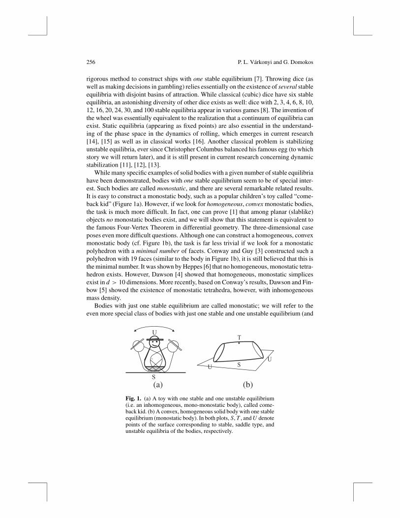
While many specific examples of solid bodies with a given number of stable equilibriahave been demonstrated, bodies with one stable equilibrium seem to be of special inter-est. Such bodies are called monostatic, and there are several remarkable related results.It is easy to construct a monostatic body, such as a popular children’s toy called “come-back kid” (Figure 1a). However, if we look for homogeneous, convex monostatic bodies,the task is much more difficult. In fact, one can prove [1] that among planar (slablike)objects no monostatic bodies exist, and we will show that this statement is equivalent tothe famous Four-Vertex Theorem in differential geometry. The three-dimensional caseposes even more difficult questions. Although one can construct a homogeneous, convexmonostatic body (cf. Figure 1b), the task is far less trivial if we look for a monostaticpolyhedron with a minimal number of facets. Conway and Guy [3] constructed such apolyhedron with 19 faces (similar to the body in Figure 1b), it is still believed that this isthe minimal number. It was shown by Heppes [6] that no homogeneous, monostatic tetra-hedron exists. However, Dawson [4] showed that homogeneous, monostatic simplicesexist in d > 10 dimensions. More recently, based on Conway’s results, Dawson and Fin-bow [5] showed the existence of monostatic tetrahedra, however, with inhomogeneousmass density.
Bodies with just one stable equilibrium are called monostatic; we will refer to theeven more special class of bodies with just one stable and one unstable equilibrium (and
S
S
UT
U
U
(a) (b)
Fig. 1. (a) A toy with one stable and one unstable equilibrium(i.e. an inhomogeneous, mono-monostatic body), called come-back kid. (b) A convex, homogeneous solid body with one stableequilibrium (monostatic body). In both plots, S, T , and U denotepoints of the surface corresponding to stable, saddle type, andunstable equilibria of the bodies, respectively.

Static Equilibria of Rigid Bodies 257
no other equilibria) as “mono-monostatic.” While in the case of two-dimensional bodiesbeing monostatic implies being mono-monostatic (and vice versa), the three-dimensionalcase is more complicated: a monostatic body could have, in principle, any number ofunstable equilibria. V. I. Arnold pointed out [17] that the existence of homogeneous,convex mono-monostatic bodies is an interesting question. Although the nonexistenceof such objects in two dimensions is known [1], Arnold nevertheless conjectured thattheir three-dimensional counterparts existed.
Our primary goal is to find a meaningful classification scheme encompassing allpossible combinations of equilibria for convex, homogeneous bodies (this will be donein Section 2) and to identify all empty and non-empty classes in this scheme. Thebackbone of our argument (discussed in Sections 3–5) is simple: we will give an explicitconstruction for a three-dimensional mono-monostatic body (thus confirming Arnold’sconjecture) and deduce the existence of bodies in other classes by complete induction.In the inductive steps, small portions are sliced off the bodies, increasing the number oftheir equilibria. The same idea appears in the construction of Zocchihedra (dice with 100facets), which are constructed this way from spheres [8]. Finally, Section 6 summarizesand illustrates the material by showing statistical results on pebbles as well as discussingvarious shapes of dice.
2. The Global Classification Scheme and Formulation of the Main Statements
In this section we introduce a global classification scheme for convex, homogeneousbodies based on the number and type of their equilibria, and we will use the notationsof this scheme to formulate all of our principal claims.
A homogeneous, convex 3D-body can be uniquely defined in a spherical coordinatesystem as the scalar distance R(θ ,ϕ) measured from the center of gravity G. The singular(fixed) points of the gradient vector field of R correspond to static equilibria: the typicalcases are
(1) stable node(2) unstable node(3) saddle-type singular points,
corresponding to nondegenerated minima, maxima, and saddle points of R(θ, ϕ), re-spectively. Bodies with degenerated singular points are not investigated in this paper.
The case of two-dimensional bodies is more transparent: the distance R(ϕ) is just afunction of one variable; minima and maxima of R (i.e. stable and unstable nodes of thegradient flow) always emerge in pairs, saddles do not occur.
Our classification of bodies is based on
Definition 1. We call two convex, homogeneous bodies equivalent if for all listed typesthe number of singular points is equal.
Hence in the two-dimensional case the number of minima uniquely characterizes anequivalence class:
258 P. L. Varkonyi and G. Domokos
Definition 2. Class {i} (i = 0, 1, 2, . . .) contains all homogeneous, convex, two-dimen-sional bodies with i stable and i unstable equilibria.
As simple examples we mention the ellipse in class {2} and regular n-gons in class {n}.In the case of three-dimensional bodies (i.e. in the case of two-dimensional flows),
Poincare indices can be associated with the three listed singularities; the indices are+1,+1, and −1, respectively [10]. We appeal to the
Poincare-Hopf Theorem [9]. The index of a vector field (i.e. the sum of the indices as-sociated with the singularities) with finitely many zeros on a compact, oriented manifoldis the same as the Euler characteristics of the manifold, implying that the sum S of thePoincare indices depends only on the topology of the manifold; in the case of a sphere,we have S = 2.
Thus, we have
Definition 3. In three dimensions, class {i, j}, (i, j = 0, 1, . . .) contains all homoge-neous, convex bodies with i stable equilibria (minima) and j unstable equilibria (max-ima). (Henceforth we use “stable equilibrium” to refer to a nondegenerate local minimum,“unstable equilibrium” to refer to a nondegenerate local maximum, and “saddle” to referto a nondegenerate saddle point of R.)
Due to the Poincare-Hopf Theorem, bodies in class {i, j} have k = i + j −2 saddles.As simple examples we mention the general ellipsoid with three different axes in class{2, 2}, the regular tetrahedron in class {4, 4}, and the cube in class {6, 8}. By applyingthe classification schemes of Definitions 1, 2, and 3, we can now formulate our claims.
The equivalence classes {0}, {0, i}, and {i, 0} (i = 0, 1, 2, . . .) are trivially empty:our vector field has been derived from a scalar potential; hence it has to contain at leastone stable and one unstable node, corresponding to the global maximum and minimumof R. We will concentrate on the nontrivially non-empty classes {i} and {i, j} withi, j = 1, 2, . . .. In the planar case we already mentioned simple examples for all classes{i} with i > 1. Class {1} is less trivial: our intuition suggests that it may be empty and,in fact, [1] proves
Theorem 1. Class {1} is empty.
That is, convex, homogeneous, rigid, planar slablike bodies, resting on a horizontalsurface in the presence of a uniform, vertical gravity field have at least two stableequilibria (in other words, homogeneous monostatic bodies, and thus homogeneousmono-monostatic bodies, do not exist in two dimensions).
At first sight it is not clear what would be the spatial analogy of Theorem 1: theemptiness of the classes {1, 1} (mono-monostatic), {1, i} (monostatic), or {i, 1} are allcandidate statements. As V. I. Arnold pointed out [17], the essence of Theorem 1 is thatin two dimensions the minimal number of equilibria is four. The only three-dimensionalbodies with fewer than four equilibria are the mono-monostatic ones, i.e. class {1, 1}.(For example, the monostatic body in Figure 1b represents class {1, 2}, and it has onestable, two unstable, and one saddle-type equilibrium, four equilibria altogether.) Hence
Static Equilibria of Rigid Bodies 259
the three-dimensional analogy of Theorem 1 would be the emptiness of class {1, 1}.Arnold hinted that a 3-D counterexample, with fewer than four equilibria (i.e. a mono-monostatic body) may nevertheless exist. With our current notation this would mean thatclass {1, 1} is non-empty.
This idea appears to be rather intriguing since (as we show in Appendix B) Theorem 1is equivalent to the famous
Four-Vertex (or 4V) Theorem [2]. The curvature of a simple (not self-intersecting),smooth, convex, closed, planar curve always has at least four local extrema, if its extremaare isolated. (The same statement is true for concave curves too, but it has, to ourknowledge, no mechanical analogy.)
The generalization of the 4V theorem for surfaces is far from trivial: it is not clearwhat should be the analogy of the planar curvature. Our goal is to show that, at least inthis mechanical analogue, the spatial generalization fails: we construct explicit, three-dimensional counterexamples with only two equilibria to prove
Theorem 2. Class {1, 1} is non-empty.
Thus we confirm Arnold’s initial guess. We will proceed in Section 3 by constructing thetwo-parameter family R(θ, ϕ, c, d) of smooth, closed surfaces in a spherical (r, θ, ϕ)polar coordinate system. The intuitive idea behind this construction, as we will pointout, is rooted in the proof of Theorem 1. Although the planar argument does not workin 3-D, it helps to prove the opposite statement. The bodies representing class {1, 1} areembedded in this family, and Section 4 defines the intervals of the two parameters c andd associated with them. The existence of appropriate values for c and d is demonstratedanalytically, and one solution is determined numerically. Appendix A contains the proofof some lemmas. In Section 5 we will use complete induction (based on the idea ofColumbus’s egg) to prove the natural generalization of Theorem 2 in the form of
Theorem 3. Class {i, j} is non-empty for i, j > 0.
3. Construction of a Surface
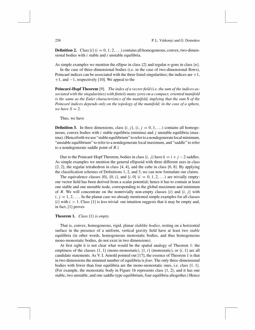
In Sections 3 and 4 we provide an explicit construction for a homogeneous, convex,mono-monostatic body, i.e. an element of class {1, 1}. As the first step, in this sectionwe define a suitable two-parameter family of surfaces R(θ, ϕ, c, d) in the sphericalcoordinate system (r, θ, ϕ) of Figure 2 with −π /2 < ϕ < π /2 and 0 ≤ θ ≤ 2π ,or ϕ = ±π /2 and no θ coordinate, while c > 0 and 0 < d < 1 are parameters. Thesolid, homogeneous body bounded by R(θ, ϕ, c, d) is denoted byB. In Section 4 we willidentify a range of the two parameters whereB is in {1, 1}, i.e. it is convex, homogeneous,and has only two equilibria. Before starting the construction, the proof of the emptinessof class {1} in the planar case is sketched (cf. [1]). This proof does not work it the 3-Dcase; however, it suggests how to prove the opposite in 3-D, i.e., how to construct arepresentative of class {1, 1}.
260 P. L. Varkonyi and G. Domokos
�
�
P
�
S
Fig. 2. A P point of the R(θ, ϕ) surfaceand the spherical coordinate system.N andS denote the “north pole” and the “southpole” of the surface.
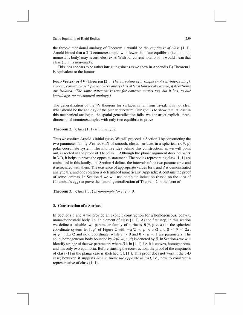
To prove the emptiness of class {1} indirectly, consider a convex, homogeneous planar“body” B and a polar coordinate system with origin at the center of gravity of B. Let thedifferentiable function R(ϕ)denote the boundary ofB. As demonstrated in [1], nondegen-erated stable/unstable equilibria of the body correspond to local minima/maxima of R(ϕ).Assume that B is in class {1}, i.e., R(ϕ) has only one local maximum and one local min-imum. In this case there exists exactly one value ϕ = ϕ0 for which R(ϕ0) = R(ϕ0+π);moreover, R(ϕ) > R(ϕ0) if π > ϕ − ϕ0 > 0, and R(ϕ) < R(ϕ0) if −π < ϕ − ϕ0 < 0(see Figure 3a). The straight line ϕ = ϕ0 (and ϕ = ϕ0 + π) passing through the originO cuts B into a “thin” (R(ϕ) < R(ϕ0) and a “thick” (R(ϕ) > R(ϕ0) part. This impliesthat O cannot be the center of gravity, i.e., it contradicts the initial assumption.
Similar to the planar case, a 3-D body in class {1, 1} can be cut into a “thin” anda “thick” part by a closed curve on its boundary, along which R(θ, ϕ) is constant. Ifthis separatrix curve happens to be planar, its existence leads to contradiction (if, for
(a)
O
(b)
j0
maximumof R
minimumof R R( )j0
R( )=
=
j p
j0
0
+
R( )
R( )j,q
sphereequator
N
S
R(0 ),q
Fig. 3. (a) Example of a convex, homogeneous, planar body boundedby R(ϕ). If R has only two local extrema, the body can be cut into a“thin” and a “thick” half by the line ϕ = ϕ0. Its center of gravity is onthe “thick” side; in particular, it cannot be in O. (b) A 3-D body (dashedline) cut into a “thin” and a “thick” half by a tennis ball-like space curve(dotted line) along which R = R0. The continuous line shows a sphereof radius R0, which also contains this curve.

Static Equilibria of Rigid Bodies 261
example, it is the “equator” ϕ = 0 and ϕ > 0/ϕ < 0 are the thick/thin halves, the centerof gravity should be on the upper (ϕ > 0) side of the origin). However, in the case ofa generic, spatial separatrix the above argument does not apply any more. In particular,the curve can be similar to the ones on the surfaces of tennis balls (Figure 3b). In thiscase the “upper” thick (“lower” thin) part is partially below (above) the equator; thus itis possible to have the center of gravity at the origin. Our construction will be of thistype.
Conveniently, R can be decomposed in the following way:
R(θ, ϕ, c, d) = 1+ d ·R(θ, ϕ, c), (1)
whereR denotes the type of deviation from the unit sphere. “Thin”/“thick” parts of thebody are characterized by negativeness/positiveness ofR (i.e., the separatrix betweenthe thick and thin portions will be given byR = 0), while the parameter d is a measureof the “flatness” of the surface. We will chose adequately small values of d to make thesurface convex.
Our next goal is to define a suitable functionR. We will have the maximum/minimumpoints of R (R = ±1) at the north/south pole (ϕ = ±π /2). The shapes of the thickand thin portions of the body are controlled by the parameter c: for c 1 the separatrixwill approach the equator; for smaller values of c the separatrix will become similar tothe curve on the tennis ball.
Consider the following smooth, one-parameter mapping f (ϕ, c): (−π /2, π /2) →(−π /2, π /2):
f (ϕ, c) = π ·[
e[ ϕ
πc+ 12c ] − 1
e1/c − 1− 1
2
]. (2)
For very large values of the parameter (c 1), this mapping is almost the identity;however, if c is close to 0, the deviation from linearity is large (cf. Figure 4).
Based on f , we define the related maps (Figure 5):
f1(ϕ, c) = sin( f (ϕ, c)), (3)
f2(ϕ, c) = − f1(−ϕ, c). (4)
�
�/2
-�/2
-�/2
�/2
c=1/8c=
1/4c=
1
c>>1
f
Fig. 4. The f (ϕ) function at some valuesof c.

262 P. L. Varkonyi and G. Domokos
�
1
-�/2
-1
�/2sin(�)
f2( )�
f1( )�
Fig. 5. The f1(ϕ), f2(ϕ), and sin(ϕ) func-tions at c = 1/3.
These two functions are used to obtain
R(0, ϕ, c) = R(π, ϕ, c) = f1(ϕ, c), (5)
R(π /2, ϕ, c) = R(3π /2, ϕ, c) = f2(ϕ, c). (6)
The planes ϕ = 0 and ϕ = π /2 will provide two planes of symmetry of the separatrixof Figure 3b; a big portion of section (5) of B lies in the thick part, while the majority ofsection (6) is in the thin part. The function
a(θ, ϕ, c) = cos2(θ) · (1− f 21 )
cos2(θ)(1− f 21 )+ sin2(θ) · (1− f 2
2 )
= 1
1+ tan2(θ)cos2( f (ϕ,c))
cos2( f (−ϕ,c)), where |ϕ| < π /2, (7)
(illustrated in Figure 6) is used to construct R as a “weighted average”-type function
�
1
�/2-�/2
�=0
�=�/8
�=2�/8�=3�/8
�=4�/8
1
�-�
� �/2
�=0
� -�/2
a a
�
Fig. 6. Sections of the a(θ, ϕ) function at c = 1.

Static Equilibria of Rigid Bodies 263
�
1
-�/2
-1
�/2
�=4�/8
�=3�/8
�=2�/8
�=�/8
�=0
�R
Fig. 7. Sections of theR(θ, ϕ) functionat constant values of θ ; c = 1/4.
of f1 and f2 in the following way (cf. Figure 6):
R(θ, ϕ, c) =
a · f1 + (1− a) · f2 if |ϕ| < π /21 if ϕ = π /2−1 if ϕ = −π /2
. (8)
The choice of the function a ensures on the one hand the gradual transition from f1 to f2
if θ is varied between 0 and π /2; on the other hand, it was chosen to result in the desiredshape of thick/thin halves of the body (illustrated in Figure 3b).
The function R defined by equations (1)–(8) is illustrated in Figure 8 for intermediatevalues of c and d . Before we identify suitable ranges of the parameters where the cor-responding body B is convex and mono-monostatic (Section 4), let us briefly commenton the effect of c. For c 1, the constructed surface R = 1 + dR is separated bythe ϕ = 0 equator into two unequal halves: the upper (ϕ > 0) half is “thick” (R > 1)and the lower (ϕ < 0) half is “thin” (R < 1). By decreasing c, the line separatingthe “thick” and “thin” portions becomes a space curve; thus the thicker portion movesdownward and the thinner portion upward. As c approaches zero, the upper half of thebody becomes thin and the lower one becomes thick (cf. Figure 9).
Fig. 8. Plot of B if c = d = 1/2.

264 P. L. Varkonyi and G. Domokos
1
(a) (b)
OO
N
S
N
S
j=
p/2
j=q=0
j=0q=p
Fig. 9. (a) Side view of B if c 1 (and d ≈ 1/3). Notethat R > 0 if ϕ > 0 and R < 0 if ϕ < 0. (b) Spatialview of B if c 1. Here, R > 0 typically for ϕ < 0and vice versa.
4. Calibration of the Parameters and the Main Result
In this section we identify the suitable ranges of the parameters c and d where the bodyB is convex and has only two equilibria; thus we complete the proof of Theorem 2.
As already mentioned in the introduction, if the center of gravity G of a convexbody B (bounded by the surface R) is at the origin of the spherical coordinate system,then singular points of R correspond to equilibria of the body in a mutually one-to-onemanner: those and only those positions are equilibria where one of the singular pointsis in contact with the underlying surface. The planar analogue of this statement hasalready been utilized in the proof of Theorem 1 (cf. [1]) and the spatial extension israther straightforward, so we do not discuss it here. We merely note that singular pointsof R in the spatial case are defined by the conditions
∂R(θ, ϕ, c, d)
∂ϕ= ∂R(θ, ϕ, c, d)
∂θ= 0, (9)
except at the “poles” (ϕ = ±π /2), where the corresponding condition is
∂R(θ, ϕ, c, d)
∂ϕ
∣∣∣∣ϕ=±π /2
= 0, for any θ. (10)
We show in Lemma A.1 (Appendix A) that the function R, defined in equations (1)–(8)of the previous section, has no more than two singular points, namely the poles N and S(cf. Figure 2).
In the forthcoming part of this section we show that B has the desired properties atappropriate values of the parameters: c and d can be chosen in such a way that
• the center of gravity G coincides with the origo O of the coordinate system, and• B is convex.
Static Equilibria of Rigid Bodies 265
d
h’(c, )0
h’(c, )d0
c2c
1
d0
d0
c
c
F c2( )
F d1( )
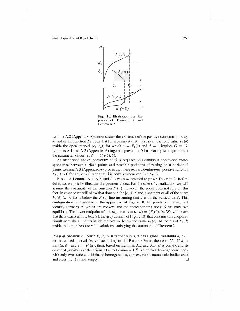
Fig. 10. Illustration for theproofs of Theorem 2 andLemma A.2.
Lemma A.2 (Appendix A) demonstrates the existence of the positive constants c1 < c2,δ0 and of the function F1, such that for arbitrary δ < δ0 there is at least one value F1(δ)
inside the open interval (c1, c2), for which c = F1(δ) and d = δ implies G ≡ O .Lemmas A.1 and A.2 (Appendix A) together prove that B has exactly two equilibria atthe parameter values (c, d) = (F1(δ), δ).
As mentioned above, convexity of B is required to establish a one-to-one corre-spondence between surface points and possible positions of resting on a horizontalplane. Lemma A.3 (Appendix A) proves that there exists a continuous, positive functionF2(c) > 0 for any c > 0 such that B is convex whenever d < F2(c).
Based on Lemmas A.1, A.2, and A.3 we now proceed to prove Theorem 2. Beforedoing so, we briefly illustrate the geometric idea. For the sake of visualization we willassume the continuity of the function F1(d); however, the proof does not rely on thisfact. In essence we will show that drawn in the [c, d] plane, a segment or all of the curveF1(d) (d < δ0) is below the F2(c) line (assuming that d is on the vertical axis). Thisconfiguration is illustrated in the upper part of Figure 10. All points of this segmentidentify surfaces R, which are convex, and the corresponding body B has only twoequilibria. The lower endpoint of this segment is at (c, d) = (F1(0), 0). We will provethat there exists a finite box (cf. the grey domain of Figure 10) that contains this endpoint;simultaneously, all points inside the box are below the curve F2(c). All points of F1(d)inside this finite box are valid solutions, satisfying the statement of Theorem 2.
Proof of Theorem 2. Since F2(c) > 0 is continuous, it has a global minimum d0 > 0on the closed interval [c1, c2] according to the Extreme Value theorem [22]. If d <
min[δ0, d0] and c = F1(d), then, based on Lemmas A.2 and A.3, B is convex and itscenter of gravity is at the origin. Due to Lemma A.1 B is a convex homogeneous bodywith only two static equilibria, so homogeneous, convex, mono-monostatic bodies existand class {1, 1} is non-empty.
266 P. L. Varkonyi and G. Domokos
Numerical analysis shows that d must be very small (d < 5·10−5) to satisfy convexitytogether with the other restrictions, so the created object is very similar to a sphere. (Inthe admitted range of d the other parameter is approximately c ≈ 0.275.) This showsthat physical demonstration of such an object might be problematic. Nevertheless, othersuch bodies, rather different from the sphere, may exist; it is an intriguing question whatis the maximal possible deviation from the sphere.
We remark that [1] also demonstrates the statement analogous to Theorem 1 forclosed, homogeneous, planar thin wires. The 3-D analogue for convex, homogeneousspatial thin shells is again false, which can be proven in the same way as Theorem 2.
5. The Egg of Columbus and Complete Induction
According to some accounts, Christopher Columbus attended a dinner given in his honorby a Spanish gentleman. Columbus asked the gentlemen in attendance to make an eggstand on one end. After the gentlemen successively tried to and failed, they stated that itwas impossible. Columbus then placed the egg’s small end on the table, breaking the shella bit, so that it could stand upright. Columbus then stated that it was “the simplest thingin the world. Anybody can do it, after he has been shown how!” The egg of Columbushas become a metaphor for natural simplicity. In this section we prove Theorem 3 byinduction. Our inductive argument is as simple as the egg of Columbus—and not justmetaphorically.
Theorem 2 (proven in the previous sections) asserts the non-emptiness of class {1, 1}.Assume that class {i, j} is non-empty. If we can find a way to add one minimum whilekeeping the number of maxima constant (and vice versa) by small perturbations notviolating the convexity of the body, then the non-emptiness of all classes {i + 1, j} and{i, j + 1} (i, j > 0), and thus Theorem 3 is proven. The first, naive interpretation ofthe Columbus story is that he turned an unstable equilibrium point into a stable one.However, a closer look at the egg reveals that Columbus did something more complex.Based on the superficial account, we cannot decide which of the following scenarioswere actually realized (supposing that the egg had a perfect rotational symmetry):
(i) If Columbus hit the table with the egg so that the symmetry axis of the egg was exactlyvertical, then by breaking the shell at the unstable equilibrium point (maximum) heproduced a small flat area containing one stable equilibrium point in the middle anda circle of degenerated balance points at the borderline of the flat part. This scenariois illustrated in Figure 11b.
(ii) If the axis was somewhat tilted, then by breaking the shell at the unstable equilibriumpoint (maximum), he produced a small flat area containing one stable equilibriumpoint (minimum) inside the flat part and one saddle and a maximum at the borderline.This scenario is illustrated in Figure 11c.
Needless to say, scenario (ii) is exactly what we need to produce an additional stableequilibrium without creating new maxima. Since Columbus’s algorithm applies onlyfor a degenerate maximum with rotational symmetry, we will use a slightly differenttechnique to produce additional maxima and minima one by one in the vicinity of typicalequilibrium points.

Static Equilibria of Rigid Bodies 267
U0
c
U0
UST U0
(a) (b) (c)
Fig. 11. Analysis of the egg of Columbus. (a) Gradient flow on theoriginal egg near the tip U0 (unstable equilibrium point). (b) Hitting thetable with vertical egg axis: modified flow containing one minimum at U0
and a set χ of degenerated equilibria. (c) Hitting the table with slightlytilted egg axis: modified flow containing one minimum (S), one saddle(T ), and one maximum (U ). Grey indicates the flat part of the egg.
5.1. Increasing the Number of Stable Equilibria by One
Consider a (smooth) stable equilibrium point (local minimum) S0 of the surface R and apoint S1 on the R = R(S0) sphere, by distance δ 1 from S0 (Figure 12a). The tangentplane of this sphere at S1 divides B into two parts, and we remove the small cap. Themodified function R, corresponding to the truncated body, still has a local minimumat S0 and a new local minimum at S1. A new saddle point T also emerges, which is astraightforward consequence of the Poincare-Hopf theorem. This situation is illustratedin Figure 12a, and the gradient flow is shown for the unperturbed and perturbed body inFigures 13a and 13b, respectively.
Notice that the truncation of the body moves the center of gravity G of B (and thusall nondegenerate critical points) by ε ≤ o(δ4), so this effect can be neglected. It is alsoworth mentioning that the truncated body is only weakly convex, because of its flat part.Strong convexity can be restored by an adequate, arbitrary small perturbation of R.
5.2. Increasing the Number of Unstable Equilibria by One
Again, consider a stable equilibrium point S0. Draw a very flat cone of revolution (δ 1,see Figure 12b), with rotation axis GS0 and its peak at S0. The cone again cuts B into twoparts, and we again remove the small one. The modified function R has a local maximumin S0; it decreases radially until it reaches a circle χ of nonisolated equilibria and beyondthe circle, it increases again (see Figure 12b, Figure 13c).
The effect of the deviation of G on the number and type of equilibria can again beneglected if δ is small, with the exception of χ , which is degenerated and structurallyunstable. Typically, G ′ is off the GS0 line; in this case χ breaks up into one isolatedminimum S1 and a saddle point T (see Figure 13d, Figure 12b). (In the nontypical casewhen G ′ happens to be on the line GS0, χ is preserved; however, it can be broken upinto a minimum and a saddle point by an adequate small perturbation of R.) Finally wehave one stable (S1), one saddle (T ), and one unstable equilibrium (S0) instead of theoriginal stable point S0.
268 P. L. Varkonyi and G. Domokos
S0
S1
G G’
Bplan
e
S0
GB
cone
c
d
(a) (b)
d
cS
1
T
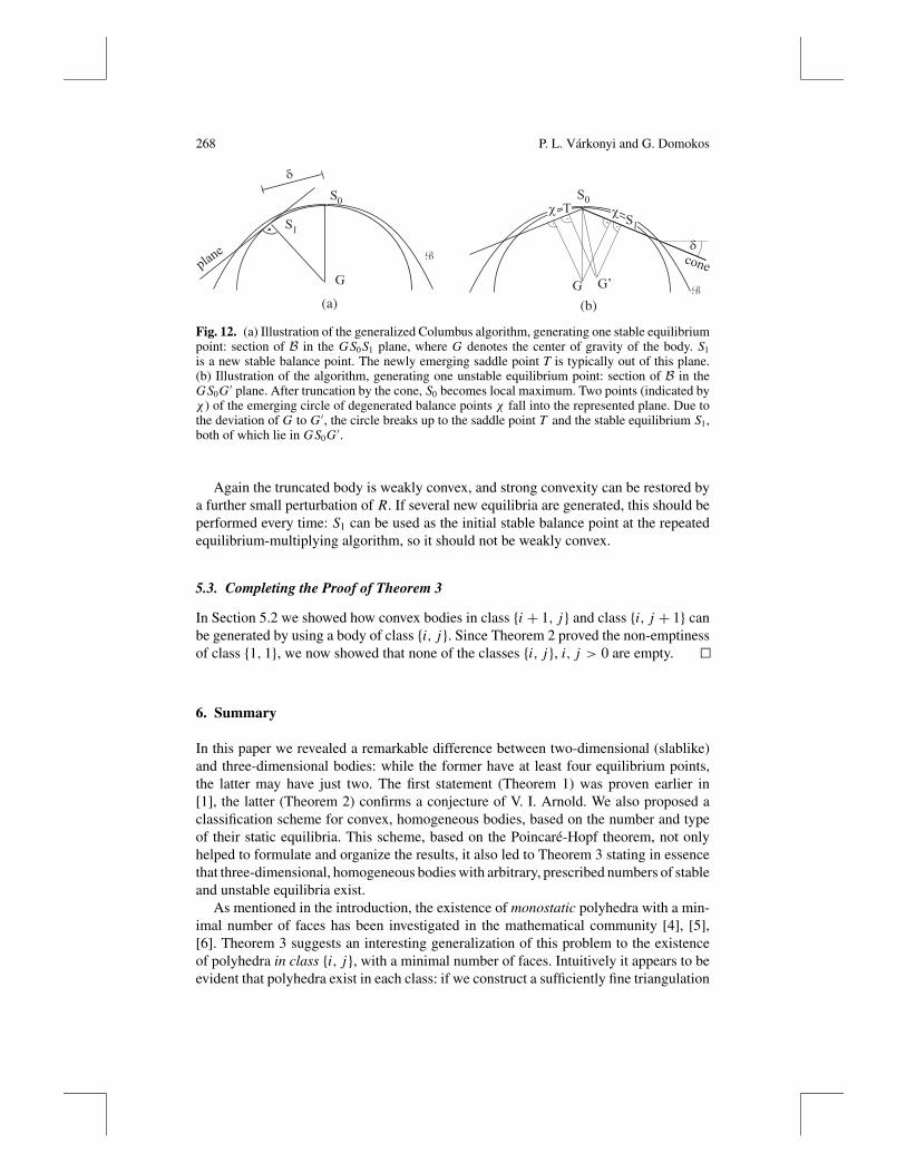
Fig. 12. (a) Illustration of the generalized Columbus algorithm, generating one stable equilibriumpoint: section of B in the GS0 S1 plane, where G denotes the center of gravity of the body. S1
is a new stable balance point. The newly emerging saddle point T is typically out of this plane.(b) Illustration of the algorithm, generating one unstable equilibrium point: section of B in theGS0G ′ plane. After truncation by the cone, S0 becomes local maximum. Two points (indicated byχ ) of the emerging circle of degenerated balance points χ fall into the represented plane. Due tothe deviation of G to G ′, the circle breaks up to the saddle point T and the stable equilibrium S1,both of which lie in GS0G ′.
Again the truncated body is weakly convex, and strong convexity can be restored bya further small perturbation of R. If several new equilibria are generated, this should beperformed every time: S1 can be used as the initial stable balance point at the repeatedequilibrium-multiplying algorithm, so it should not be weakly convex.
5.3. Completing the Proof of Theorem 3
In Section 5.2 we showed how convex bodies in class {i + 1, j} and class {i, j + 1} canbe generated by using a body of class {i, j}. Since Theorem 2 proved the non-emptinessof class {1, 1}, we now showed that none of the classes {i, j}, i, j > 0 are empty.
6. Summary
In this paper we revealed a remarkable difference between two-dimensional (slablike)and three-dimensional bodies: while the former have at least four equilibrium points,the latter may have just two. The first statement (Theorem 1) was proven earlier in[1], the latter (Theorem 2) confirms a conjecture of V. I. Arnold. We also proposed aclassification scheme for convex, homogeneous bodies, based on the number and typeof their static equilibria. This scheme, based on the Poincare-Hopf theorem, not onlyhelped to formulate and organize the results, it also led to Theorem 3 stating in essencethat three-dimensional, homogeneous bodies with arbitrary, prescribed numbers of stableand unstable equilibria exist.
As mentioned in the introduction, the existence of monostatic polyhedra with a min-imal number of faces has been investigated in the mathematical community [4], [5],[6]. Theorem 3 suggests an interesting generalization of this problem to the existenceof polyhedra in class {i, j}, with a minimal number of faces. Intuitively it appears to beevident that polyhedra exist in each class: if we construct a sufficiently fine triangulation

Static Equilibria of Rigid Bodies 269
S0
S0
S1 T
(a) (b)
S0
T
(c) (d)
c
S0 S
1
Fig. 13. Gradient flow of R on the surface of B. (a) Small vicinity ofa local minimum S0 of R. (b) The body is truncated along a plane. Asecond minimum S1 and a saddle point T occur. (c) The body is truncatedalong a cone. S0 becomes a local maximum, and a circle χ of nonisolatedsingular points emerges on the cone. (d) The deviation of the center ofgravity perturbs R. The structurally unstable circle typically breaks up toa minimum S1 and a saddle point T . Grey indicates the truncated part ofthe surface.
on the surface of a smooth body in class {i, j}with vertices at unstable equilibria, edges atsaddles and faces at stable equilibria, then the resulting polyhedron will—at sufficientlyhigh mesh density and appropriate mesh ratios—“inherit” the class of the approximatedsmooth body. It also appears to be true that if the topological inequalities 2i ≥ j + 4and 2 j ≥ i + 4 are valid, then we can have “minimal” polyhedra, where the number ofstable equilibria equals the number of faces, the number of unstable equilibria equalsthe number of vertices, and the number of saddles equals the number of edges. Muchmore puzzling appear to be the polyhedra in classes not satisfying the above topologi-cal inequalities: a special case of these polyhedra are monostatic ones; however, manyother types belong here as well. In particular, it would be of special interest to know theminimal number of faces of a polyhedron in class {1, 1}.

270 P. L. Varkonyi and G. Domokos
The relationship between mathematical proof of existence and the physical world isfar from trivial. In some cases the physical existence of solutions seems to be evident;nevertheless it is extremely hard to prove existence in the mathematical model, as is thecase with the Navier-Stokes equations [21]. Our problem appears to be of the oppositecharacter: the presented mathematical proof was not long, nor did it require complicatedtools. Nevertheless, physical intuition fails in this problem. Our experience stronglysuggests that all convex, homogeneous bodies have at least two stable equilibria andthus four equilibria altogether. Where does this intuition originate? In the introductionwe mentioned dice as the probably earliest manmade objects the essence of which isto possess discrete, multiple stable equilibria. As games evolved, a large variety of dicehave been fabricated, several ones being regular platonic solids or direct descendantsthereof. Traditionally, dice having only one stable equilibrium were regarded as illegal(inhomogeneous), called “loaded” or “gaffed.” It is a difficult mathematical challengeto construct a loaded tetrahedral die that is monostatic; this problem is addressed byDawson and Finbow [5].
Not only manmade objects have the property of often possessing multiple stableequilibria. There exist objects in nature in abundant numbers that probably come closestto the mathematical abstraction of a convex, homogeneous body: pebbles on the seacoast.Pebbles are divided into four groups based on their morphology [18]:
1. oblate (ellipsoidal disk)2. equant (sphere)3. bladed (circular disk)4. prolate (roller, rod).
All these groups can be regarded as limit shapes, resulting from multimillion-year abra-sion processes during which pebbles become increasingly smooth; in geological terms,their roundness is growing [19]. Apparently, the morphology groups 1 and 3 containflat pebbles with at least two stable equilibria, and group 4 has at least two unstableequilibria, so mono-monostatic bodies of class {1, 1} can be found only in group 2,among “spherical” objects. This is in good agreement with Sections 3 and 4, where weconstructed a mono-monostatic body with minimal deviation from the sphere. How-ever, the “Columbus-algorithm” of Section 5 suggests that almost-spherical objects areparticularly sensitive to small perturbations of shape, which may often produce ad-ditional equilibrium points in pitchfork-like or saddle-node bifurcations. So, even ifmono-monostatic pebbles exist temporarily, it is very likely that the number of theirequilibria is increased even by a small amount of abrasion. While this reasoning impliesthat pebbles in class {1, 1} are extremely rare, it also tells us that class {2, 2} might bedominant, since it can occur in all four morphology classes.
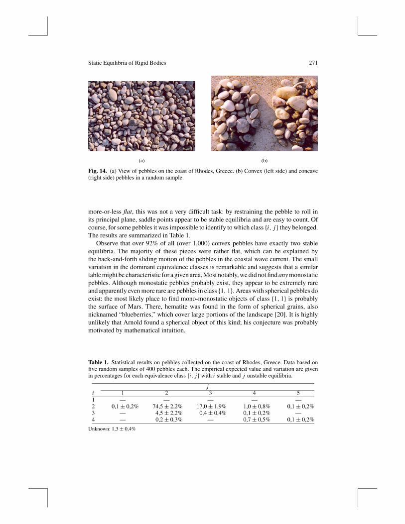
We conducted a simple statistical experiment: we collected five random samples of400 pebbles in an area of ca. 15x50 meters along the coast of Rhodes, Greece (Figure 14a).In the first step, convex and non-convex pebbles were separated; their ratio was almostconstant 51:49 (Figure 14b). In the second step the convex pebbles were classifiedaccording to the scheme of Definition 1 and Definition 3. The number of stable equilibriais relatively easy to identify. We used simple considerations and hand-held experimentsto find the number of unstable equilibria. Since the vast majority of the pebbles was
Static Equilibria of Rigid Bodies 271
(a) (b)
Fig. 14. (a) View of pebbles on the coast of Rhodes, Greece. (b) Convex (left side) and concave(right side) pebbles in a random sample.
more-or-less flat, this was not a very difficult task: by restraining the pebble to roll inits principal plane, saddle points appear to be stable equilibria and are easy to count. Ofcourse, for some pebbles it was impossible to identify to which class {i, j} they belonged.The results are summarized in Table 1.
Observe that over 92% of all (over 1,000) convex pebbles have exactly two stableequilibria. The majority of these pieces were rather flat, which can be explained bythe back-and-forth sliding motion of the pebbles in the coastal wave current. The smallvariation in the dominant equivalence classes is remarkable and suggests that a similartable might be characteristic for a given area. Most notably, we did not find any monostaticpebbles. Although monostatic pebbles probably exist, they appear to be extremely rareand apparently even more rare are pebbles in class {1, 1}. Areas with spherical pebbles doexist: the most likely place to find mono-monostatic objects of class {1, 1} is probablythe surface of Mars. There, hematite was found in the form of spherical grains, alsonicknamed “blueberries,” which cover large portions of the landscape [20]. It is highlyunlikely that Arnold found a spherical object of this kind; his conjecture was probablymotivated by mathematical intuition.
Table 1. Statistical results on pebbles collected on the coast of Rhodes, Greece. Data based onfive random samples of 400 pebbles each. The empirical expected value and variation are givenin percentages for each equivalence class {i, j} with i stable and j unstable equilibria.
ji 1 2 3 4 51 — — — — —2 0,1± 0,2% 74,5± 2,2% 17,0± 1,9% 1,0± 0,8% 0,1± 0,2%3 — 4,5± 2,2% 0,4± 0,4% 0,1± 0,2% —4 — 0,2± 0,3% — 0,7± 0,5% 0,1± 0,2%
Unknown: 1,3± 0,4%

272 P. L. Varkonyi and G. Domokos
Acknowledgments
Comments from Phil Holmes, Jerry Marsden, Akos Torok, and two unknown refereeshelped to shape this paper substantially. The authors also thank Reka Domokos for hercomments and invaluable help with the pebble experiment. This work has been supportedby OTKA grant TS 049885.
Appendix A
Here we prove Lemmas A.1, A.2, and A.3, all of which have been used in the precedingproof of Theorem 2.
A.1. Singular points of R
Here we prove
Lemma A.1. The function R has no other singular point than the poles.
Proof of Lemma A.1. The poles are singular points because of the reflection-symmetryof R to the planes � = 0 and � = π /2 (cf. equation (7)).
At other points, the partial derivatives of R are determined based on equations (1)and (8). The first one is
∂R
∂θ= d
∂a
∂θ· ( f1 − f2). (11)
This partial derivative is zero if either
f2 − f1 = 0, (12)
which holds for the poles only, or
∂a
∂θ= 0, (13)
which holds if and only if θ = k · π /2. At these lines,
R(θ, ϕ) = 1+ d · fi (ϕ), i = 1+ k mod 2 (14)
(cf. equations (5) and (6)). Now we have to show that the second partial derivative isnon-zero along these lines. The second partial derivative at θ = k · π /2 (with respect toϕ) is given by
∂R
∂ϕ= d · d fi (ϕ)
dϕ, i = 1+ k mod 2, (15)
which is non-zero except at the poles. Thus, there are really no other singular points.

Static Equilibria of Rigid Bodies 273
A.2. Coincidence of the Origin with the Center of Gravity
In this subsection we show under which conditions the origin O of the coordinatesystem coincides with the center of gravity G of the body B, defined by the surface R(cf. equations (1)–(8)).
Lemma A.2. There exist positive constants c1 < c2, δ0 and a function F1 such that forarbitrary δ < δ0, (c, d) = (F1(δ), δ) implies G ≡ O and c1 ≤ F1(δ) ≤ c2.
Proof of Lemma A.2. The reflection symmetry of the body with respect to the θ = 0and θ = π /2 planes implies that G is on the vertical line ϕ ± π /2 passing through theorigin O . The vertical distance h between O and G can be expressed as a function ofthe parameters c and d:
h(c, d) =∫ 2π
0
∫ π /2−π /2
14 R(ϕ, θ, c, d)4 cosϕ sinϕ dϕ dθ
V (c, d). (16)
where V (c, d) denotes the volume of the body, and G ≡ O iff h(c, d) = 0.Equation (16) can be transformed to
h(c, d) = 1
V (c, d)
∫ 2π
0
∫ π /2
−π /2
14 (1+ dR(ϕ, θ, c))4 cosϕ sinϕdϕdθ
= 1
V (c, d)
[∫ 2π
0
∫ π /2
−π /2cosϕ sinϕdϕdθ
+ d∫ 2π
0
∫ π /2
−π /2(R + 3
2 dR2 + d2R3 + 14 d3R4) cosϕ sinϕdϕdθ
]
= 1
V (c, d)
×[0+d
∫ 2π
0
∫ π /2
−π /2(R+ 3
2 dR2+d2R3+ 14 d3R4) cosϕ sinϕdϕdθ
],
(17)
which shows that h(c, d) = 0 is equivalent to the condition
h′(c, d) =∫ 2π
0
∫ π /2
−π /2(R + 3
2 dR2 + d2R3 + 14 d3R4) cosϕ sinϕ dϕ dθ = 0,
(18)if d > 0; moreover,
sign(h(c, d)) = sign(h′(c, d)). (19)
We remark that h′(c, d) is continuous in c and d, for c > 0 and arbitrary d (d might be0 as well).
Observe that
h′(c, 0) =∫ 2π
0
∫ π /2
−π /2R cosϕ sinϕdϕdθ (20)

274 P. L. Varkonyi and G. Domokos
is positive if c approaches infinity, because
limc→∞R(θ, ϕ, c) = sin(ϕ), (21)
and the product R cosϕ sinϕ is nonnegative (see also Figure 9a).At the same time, if c→ 0, we have
limc→0
R(θ, ϕ, c) =
1 if
−π /2 < ϕ < 0, θ �= k · π /2ϕ = π /2
−π /2 < ϕ < π /2, θ = (2k + 1) · π /2
−1 if
0 < ϕ < π /2, θ �= k · π /2ϕ = −π /2
−π /2 < ϕ < π /2, θ = 2k · π /2
sin2 θ − cos2 θ if ϕ = 0
,
(22)and the productR cosϕ sinϕ is typically negative, yielding h′(c, 0) < 0 (cf. Figure 9b).
Since h′(c, 0) is continuous in c, there exist positive constants c1 < c2 such thath′(c1, 0) < 0 < h′(c2, 0) (see the lower part of Figure 10). Again, because of thecontinuity of h′(c, d), there exists a constant δ0 for which 0 < δ < δ0 implies h′(c1, δ) <
0 < h′(c2, δ). So if 0 < δ < δ0, there is a constant c1 < F1(δ) < c2 for whichh′(c0, δ) = 0. Thus, c = F1(δ) and d = δ implies that G ≡ O .
A.3. Convexity of the Body
In this part we show
Lemma A.3. There exists a continuous function F2(c) for any c > 0, so that the bodyis convex if 0 < d < F2(c).
We prepare the proof of Lemma A.3 in four parts.In Section A.3.1, a sufficient condition of local convexity is determined, based on
the Hessian of the surface in a local orthogonal coordinate system. This condition canbe applied everywhere except the poles. In Section A.3.2, some functions related to Rare extended to a closed domain and their boundedness is stated in Proposition A.3.2.Based on these results, in A.3.3 we prove Proposition A.3.3, stating convexity at regularpoints (we determine a function F2(c) and show that the surface is convex at such pointsif d < F2(c)). Finally, it is verified in Section A.3.4 that the convexity requirement isfulfilled at the poles, too; this is the statement of Proposition A.3.4.
Proof of Lemma A.3. Propositions A.3.3 and A.3.4 imply Lemma A.3.
A.3.1. A Sufficient Condition for Local Convexity at an Arbitrary Point. At anysurface point P(ϕ0, θ0), R can be expressed as z(x, y) in an x-y-z local orthogonalcoordinate system, axis z passes through the origin O (see Figure 15). A sufficient
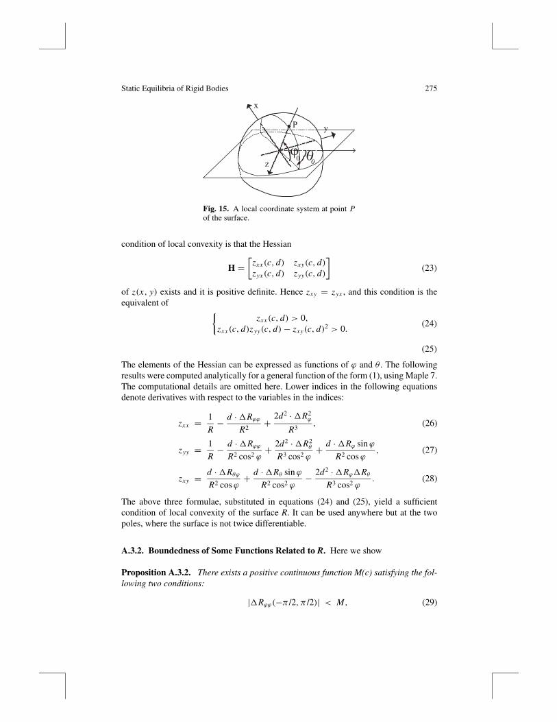
Static Equilibria of Rigid Bodies 275
yP
x
z0
�0
�
Fig. 15. A local coordinate system at point Pof the surface.
condition of local convexity is that the Hessian
H =[
zxx (c, d) zxy(c, d)zyx (c, d) zyy(c, d)
](23)
of z(x, y) exists and it is positive definite. Hence zxy = zyx , and this condition is theequivalent of {
zxx (c, d) > 0,zxx (c, d)zyy(c, d)− zxy(c, d)2 > 0.
(24)
(25)
The elements of the Hessian can be expressed as functions of ϕ and θ . The followingresults were computed analytically for a general function of the form (1), using Maple 7.The computational details are omitted here. Lower indices in the following equationsdenote derivatives with respect to the variables in the indices:
zxx = 1
R− d ·Rϕϕ
R2+ 2d2 ·R2
ϕ
R3, (26)
zyy = 1
R− d ·Rϕϕ
R2 cos2 ϕ+ 2d2 ·R2
θ
R3 cos2 ϕ+ d ·Rϕ sinϕ
R2 cosϕ, (27)
zxy = d ·RθϕR2 cosϕ
+ d ·Rθ sinϕ
R2 cos2 ϕ− 2d2 ·RϕRθ
R3 cos2 ϕ. (28)
The above three formulae, substituted in equations (24) and (25), yield a sufficientcondition of local convexity of the surface R. It can be used anywhere but at the twopoles, where the surface is not twice differentiable.
A.3.2. Boundedness of Some Functions Related to R. Here we show
Proposition A.3.2. There exists a positive continuous function M(c) satisfying the fol-lowing two conditions:
|Rϕϕ(−π /2, π /2)| < M, (29)
276 P. L. Varkonyi and G. Domokos∣∣∣∣Rϕcosϕ
∣∣∣∣ ,∣∣∣∣ Rθcos2 ϕ
∣∣∣∣ , |Rϕϕ|,∣∣∣∣Rϕθ
cosϕ
∣∣∣∣ ,∣∣∣∣Rθθcos2 ϕ
∣∣∣∣ < M if |ϕ| < π /2. (30)
We can trivially satisfy (29), but there is no such guarantee for the boundedness of theleft side of (30), since these are continuous functions on open domains; observe alsothat the denominators cosϕ of (30) converge to zero at the borders of the domains.
Proof of Proposition A.3.2. Let us define ext(φ) for a given functionφ(ϕ,�)with |ϕ| <π /2 as the same function on an extended, closed domain:
ext(φ) =
φ(ϕ,�), if |ϕ| < π /2,limϕ→π /2
φ(ϕ,�), if ϕ = π /2,
limϕ→−π /2
φ(ϕ,�), if ϕ = −π /2.(31)
The following functions
ext
(Rϕcosϕ
), ext
(Rθ
cos2 ϕ
), ext(Rϕϕ), ext
(Rϕθcosϕ
), ext
(Rθθcos2 ϕ
)(32)
trivially exist and are continuous in ϕ and θ if |ϕ| < π /2. Simultaneously, for |ϕ| < π /2,one can determine the functions in (32) analytically, based on the definition (31) to verifythe same statement.
According to our analytical computations (made with Maple 7), the correspondinglimit values exist and they are continuous in θ , which imply the continuity of the extendedfunctions (32). Because the results are quite lengthy, only one of them is presented here:
ext
(Rϕcosϕ
)∣∣∣∣ϕ=+π /2
= limϕ→π /2
Rϕcosϕ
= cos2 θ · e4/c + 1− cos2 θ
c2(e2/c − 2e1/c + 1+ cos2 θ · e4/c
−2 cos2 θ · e3/c + 2 cos2 θ · e1/c − cos2 θ)
. (33)
The denominator is never zero:
1 + cos2 θ · e4/c − 2 cos2 θ · e3/c + 2 cos2 θ · e1/c − cos2 θ − 2e1/c
= 1+ cos2 θ · (e4/c − 2e3/c + e2/c)+ 2 cos2 θ · e1/c − cos2 θ − 2e1/c + sin2 θ · e2/c
> 1+ 2 cos2 θ · e1/c − cos2 θ − 2e1/c + sin2 θ · e2/c
= sin2 θ(e2/c − 2e1/c + 1) > 0, (34)
therefore function exists and it is continuous in θ .
According to the Extreme Value Theorem [22], continuous functions on compactmanifolds are always bounded. Thus, the maximum M(c) of all the functions in (32)exists. M(c) satisfies the conditions (29) and (30) and it is continuous in c.

Static Equilibria of Rigid Bodies 277
A.3.3. The Function F2(c). Here we construct the function F2(c) such that wheneverd < F2(c), R is convex at all regular points. Subsection A.3.4 extends this result to thepoles.
Proposition A.3.3. If
d ≤ F2(c) = min
{1
25M(c),
1
2
}(35)
(where M(c) is defined in Proposition A.3.2), then R is convex at all regular points.
Proof of Proposition A.3.3. Consider the following approximations on the elements ofthe Hessian (26)–(28), using Proposition A.3.2 and (35) (observe that (35) implies 1/2 <R < 3/2):
zxx ≥ 1
R−∣∣∣∣d ·Rϕϕ
R2
∣∣∣∣+ 0 >2
3− 4d M, (36)
zyy ≥ 1
R−∣∣∣∣ d ·Rθθ
R2 cos2 ϕ
∣∣∣∣+ 0−∣∣∣∣d ·Rϕ sinϕ
R2 cosϕ
∣∣∣∣>
2
3− 4d M − 4d M · sinϕ >
2
3− 8d M,
|zxy | ≤∣∣∣∣d ·Rθϕ
R2 cosϕ
∣∣∣∣+∣∣∣∣d ·Rθ sinϕ
R2 cos2 ϕ
∣∣∣∣+∣∣∣∣2d2 ·RϕRθ
R3 cos2 ϕ
∣∣∣∣< 4d M + 4d M sinϕ + 16d2 M2 · cosϕ (37)
≤ 3d M + 16d2 M2. (38)
From inequalities (35)–(38), we have
zxx (d) >2
3− 4d M ≥ 38
75> 0, (39)
and
zxx (d)zyy(d)− zxy(d)2 > ( 2
3 − 4d M)( 23 − 8d M)− (8d M + 16d2 M2)2
≥ 28 · 7057
32 · 58> 0, (40)
i.e., the conditions of convexity (24), (25) are satisfied; the function F2(c) is continuousin c.
A.3.4. Convexity at the Poles. In this part, we prove
Proposition A.3.4. B is locally convex at the two poles if d < F2(c).

278 P. L. Varkonyi and G. Domokos
Here, local convexity is demonstrated by showing a plane, which
• contains the examined pole (N or S),• has all nearby points of the surface on the same side of the plane,• has the “inside” of B also on the same side of the plane. (We choose the origin O,
which is always an inner point of the body, to examine this condition.)
Proof of Proposition A.3.4. Consider the orthogonal coordinate system of Figure 15with ϕ0 = −π /2 and θ0 = 0. The plane z = (1 + d) contains the north pole of thesurface and all other points are on the z < 1+ d side of this plane, because
Z(ϕ, θ) = R(ϕ, θ) sinϕ < R(ϕ, θ) < 1+ d. (41)
The origin O is at z = 0 also on the z < 1 + d side. Thus, the surface is convex at thenorth pole for any value of d .
Similarly, the plane z = −1+ d contains the south pole, and the origin O is at z = 0on the z > −1+ d side. The surface is locally convex if
z(ϕ, θ) = R(ϕ, θ) sinϕ > −1+ d, (42)
for any θ if 0 < ϕ + π /2 1 and d < F2(c).We start the proof of inequality (42) with the following simple relation, which is true
for arbitrary positive M (see also (35)):
d ≤ min
{1
25M,
1
2
}<
2
3(1+ M). (43)
We increase the right side of this inequality in three steps, which are discussed below:
d <2
3(1+ M)=
13 (ϕ + π /2)2
12 (1+ M)(ϕ + π /2)2
<
13 (ϕ + π /2)2
12 (1+ M)(ϕ + π /2)2 − 1
4 M(ϕ + π /2)4
= 1− 1+ 13 (ϕ + π /2)2
1− (−1+ 12 M(ϕ + π /2)2)(−1+ 1
2 (ϕ + π /2)2)
<1+ sinϕ
1− (−1+ 12 M(ϕ + π /2)2) sinϕ
<1+ sinϕ
1−R sinϕ. (44)
The first step was obvious. In the second step we used that
− 1+ 1
3(ϕ + π /2)2 < sinϕ < −1+ 1
2(ϕ + φ/2)2, (45)
if 0 < (ϕ + π /2) 1, which is simple to derive from the Taylor expansion of sin(ϕ) atϕ = −π /2 up to the third-order term. The third step is a consequence of (cf. Figure 7
Static Equilibria of Rigid Bodies 279
and eq. (29))
R(ϕ, θ) ≤ f2(ϕ) = R(ϕ, π /2)
= −1+ 0 · (ϕ + π /2)+ 12 Rϕϕ(−π /2, π /2) · (ϕ + π /2)2 + o((ϕ + π /2)3)
< −1+ 12 M(ϕ + π /2)2, (46)
which again holds for 0 < (ϕ + π /2) 1.Eq. (44) can be rearranged as
d(1−R sinϕ) < 1+ sinϕ. (47)
Via substituting eq. (1) into (47), we get eq. (42). Thus, the surface is convex at the southpole, too.
Appendix B: The Planar Results and the Four-Vertex Theorem
In this appendix we show the following:
Lemma B.1. The 4V Theorem and Theorem 1 are equivalent.
As demonstrated in [1] and already mentioned in the introduction, Theorem 1 has anotherequivalent form.
Theorem 1A. Let the function r(α) > 0 with isolated extrema, 0 ≤ α ≤ 2π andr(0) = r(2π), determine a planar curve in a polar coordinate system (r, α). If thecenter of gravity G of the corresponding planar solid body is at the origin (0, 0), thefunction r(α) has at least four extrema. This statement holds for concave curves, too.
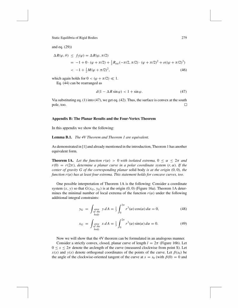
One possible interpretation of Theorem 1A is the following: Consider a coordinatesystem (x, y) so that G(xG, yG) is at the origin (0, 0) (Figure 16a). Theorem 1A deter-mines the minimal number of local extrema of the function r(α) under the followingadditional integral constraints:
yG =∫
areaof thebody
y d A = 13
∫ 2π
0r3(α) cos(α) dα = 0, (48)
xG =∫
areaof thebody
x d A = 13
∫ 2π
0r3(α) sin(α) dα = 0. (49)
Now we will show that the 4V theorem can be formulated in an analogous manner.Consider a strictly convex, closed, planar curve of length l = 2π (Figure 16b). Let
0 ≤ s ≤ 2π denote the arclength of the curve (measured clockwise from point S). Letx(s) and y(s) denote orthogonal coordinates of the points of the curve. Let β(s0) bethe angle of the clockwise-oriented tangent of the curve at s = s0 (with β(0) = 0 and
280 P. L. Varkonyi and G. Domokos
(a) (b)
S
xx
yys
b( )sa
r(a)
G
y(
)s
x s( )
Fig. 16. (a) A planar body in the polar coordinate system. (b) A con-vex, closed plane curve.
β(2π) = 2π), and let ρ(s0) denote the curvature of the curve at the same point. Since thecurve is strictly convex (ρ(s) > 0), β(s) is strictly monotonically increasing, implyingthe existence of s(β) and ρ(β) for 0 ≤ β ≤ 2π . From the monotonicity of β(s) it alsofollows that dρ/ds = 0 implies dρ/dβ = 0 and vice versa.
The 4V theorem (analogously to Theorem 1a) states that the number of local extremaof the function ρ = dβ/ds is at least four. The closing condition for the curve yields thefollowing integral constraints:
x(2π)− x(0) =∫ 2π
0
dx
dsds =
∫ 2π
0cos(β(s)) ds
=∫ β(2π)
β(0)
cos(β)
dβ/dsdβ =
∫ 2π
0
cos(β)
ρ(β)dβ = 0, (50)
y(2π)− y(0) =∫ 2π
0
dy
dsds =
∫ 2π
0sin(β(s)) ds
=∫ β(2π)
β(0)
sin(β)
dβ/sdβ =
∫ 2π
0
sin(β)
ρ(β)dβ = 0. (51)
Equations (48)–(49) and (50)–(51) are equivalent if
ρ(β) = 1
r3(α), (52)
which is a mutually one-to-one correspondence between the positive, periodic functionsr(α) and ρ(β) (α, β ∈ [0, 2π ]), determining homogeneous planar bodies and convexplane curves, respectively.
As we can see, for convex curves the 4V theorem is equivalent to the fact that 1/r3(α)
has four extrema. The latter coincide with the extrema of r(α); thus the 4V theorem forconvex curves and Theorem 1 are equivalent.
References
[1] Domokos, G., Papadopulos, J., and Ruina, A., Static equilibria of planar, rigid bodies: Is thereanything new? J. Elasticity 36 (1994), 59–66.

Static Equilibria of Rigid Bodies 281
[2] Berger, M., and Gostiaux, B., Differential geometry: Manifolds, curves and surfaces (1988),Springer, New York.
[3] Conway, J. H., and Guy, R., Stability of polyhedra, SIAM Rev. 11 (1969), 78–82.[4] Dawson, R., Monostatic simplexes, Amer. Math. Monthly 92 (1985), 541–646.[5] Dawson, R., and Finbow, W., What shape is a loaded die?, Mathematical Intelligencer 22
(1999), 32–37.[6] Heppes, A., A double-tipping tetrahedron, SIAM Rev. 9 (1967), 599–600.[7] Nowacki, H., Archimedes and ship stability. In: Passenger ship design, construction, opera-
tion and safety: Euroconference; Knossos Royal Village, Anissaras, Crete, Greece, October15–17, 2001, 335–360 (2002). Ed: Kaklis, P.D. National Technical Univ. of Athens, Depart-ment of Naval Architecture and Marine Engineering, Athens.
[8] Wikipedia, Dice, http://en.wikipedia.org/wiki/Dice[9] Arnold, V.I., Ordinary differential equations, 10th printing (1998), MIT Press, Cambridge.
[10] Farkas, M., Periodic motions (1994), Springer, New York.[11] Champneys, A.R., and Fraser, W.B., The “Indian rope trick” for a parametrically excited
flexible rod: I linearised analysis, Proc. Roy. Soc. Lond. A 456 (2000), 553–570.[12] Enikov, E., and Stepan, G., Digital stabilization of unstable equilibria, Zeitschrift fur ange-
wandte Mathematik und Mechanik 75 (1995), S111–S112.[13] Goodwine, B., and Stepan, G., Controlling unstable rolling phenomena, J. Vibration and
Control 6 (2000), 137–158.[14] Bloch, A.M., Marsden, J.E., and Zenkov, D.V., Nonholonomic dynamics, Not. Amer. Math.
Soc. 52 (2005), no. 3, 324–333.[15] Borisov, A.V., and Mamaev I.S., The rolling motion of a rigid body on a plane and a sphere:
hierarchy of dynamics, Reg. Chaot. Dynam. 7 (2002), no. 2, 177–200.[16] Chaplygin, S.A., On the rolling of a sphere on a horizontal plane, Mat. Sbornik XXIV (1903),
139–168 (in Russian).[17] Arnold, V.I., Personal communication to G. Domokos.[18] Blatt, H., Middleton, G., and Murray, R., Origin of sedimentary rocks (1972), Prentice Hall,
Englewood Cliffs, NJ.[19] Chamley, H., Sedimentology (1990), Springer, New York.[20] Squyres, S., et al., The opportunity rover’s Athena science investigation at Meridiani Planum,
Mars, Science, 306 (2004), 1698–1703.[21] Avrin, J., Global existence and regularity for the Lagrangian averaged Navier-Stokes equa-
tions with initial data in H-1/2, Commun. Pure Appl. Anal. 3 (2004), no. 3, 353–366.[22] Malik, S. C., Mathematical analysis, 2nd ed. (1992), Wiley, New York.