static analysis of 3d structure -...
TRANSCRIPT

EXAMPLE 3
Static analysis of 3D structure
Perform the analysis of the 3D structure presented in the following figure for
vertical and simplified earthquake actions.
Input data:
Consideration of diaphragm function of each floor.
Uniform distributed loading on beams:
Permanent actions g=15kN/m
Variable actions q=10kN/m.
Consideration of cracked cross-sections during the analysis.
Column cross-sections:40x60 (cm)
Beam cross-sections:
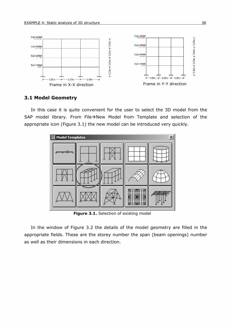
EXAMPLE 4: Static analysis of 3D structure 38
Frame in X-X direction
Frame in Y-Y direction
3.1 Model Geometry
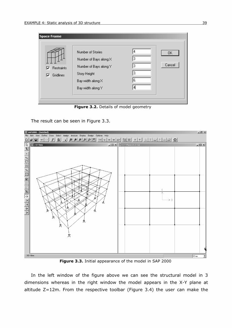
In this case it is quite convenient for the user to select the 3D model from the
SAP model library. From FileNew Model from Template and selection of the
appropriate icon (Figure 3.1) the new model can be introduced very quickly.
Figure 3.1. Selection of existing model
In the window of Figure 3.2 the details of the model geometry are filled in the
appropriate fields. These are the storey number the span (beam openings) number
as well as their dimensions in each direction.
EXAMPLE 4: Static analysis of 3D structure 39
Figure 3.2. Details of model geometry
The result can be seen in Figure 3.3.
Figure 3.3. Initial appearance of the model in SAP 2000
In the left window of the figure above we can see the structural model in 3
dimensions whereas in the right window the model appears in the X-Y plane at
altitude Z=12m. From the respective toolbar (Figure 3.4) the user can make the

EXAMPLE 4: Static analysis of 3D structure 40
selection of the desired 2D or 3D view of the model. It is recommended to have the
3D view in the left window and a plane view in the right window.
Figure 3.4. Toolbar for 2D or 3D view selection
Thus by clicking the xz icon of the previous figure (when the right window is
activated) we can see in Figure 3.5 the plane X-Z view at Y=-2m. The user can be
informed of the y-level from the window title (X-Z Plane @ Y=2). Simultaneously a
discontinuous line of light blue color appears at the 3D view window, that specifies
the location of the plane view. Changing of the Y level can take place using the up-
down arrows of Figure 3.5.
Figure 3.5. 3D and 2D views of the model. Changing levels
In order to apply the correct supports we can work as follows. First in a x-Y view
of the right window we can move to tha base (Z=0) and select all the base joints
(Figure 3.6). Then from AssignJointRestraints replace all supports with full
fixities (restrain all degrees of freedom).
EXAMPLE 4: Static analysis of 3D structure 41
Figure 3.6. Full fixities assignment at the base joints
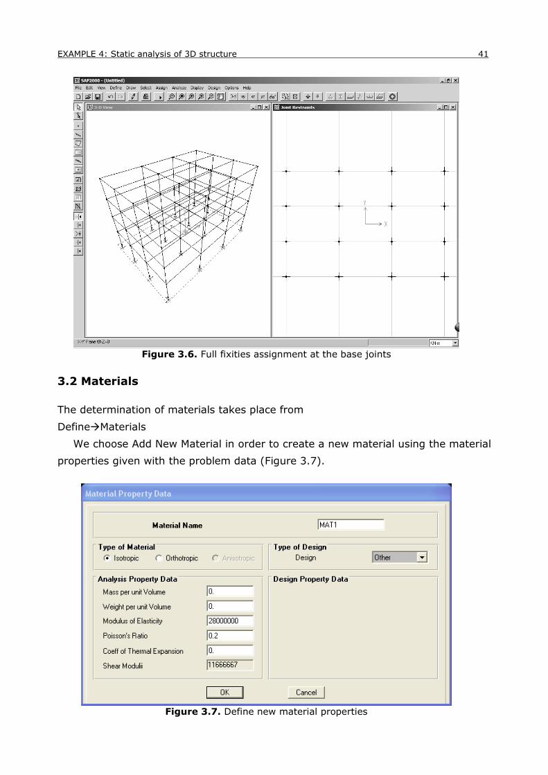
3.2 Materials
The determination of materials takes place from
DefineMaterials
We choose Add New Material in order to create a new material using the material
properties given with the problem data (Figure 3.7).
Figure 3.7. Define new material properties

EXAMPLE 4: Static analysis of 3D structure 42
3.3 Cross-sections
Cross-section determination for linear elements (Frame elements - beams,
columns) takes place from DefineFrame Sections. Columns are rectangular and
can be defined as presented in Figure 3.8 choosing the Add Rectangular option. In
this example the large dimension is given in the t3 (Depth) field. As explained in the
previous example the modification factors for resistance in flexural and shear forces
are taken equal to 0.5 of their initial value because of cracking (Figure 3.9).
Figure 3.8. Column cross-sections
Figure 3.9. Geometric characteristics of the column section and modification factors
In the same way the beam cross-sections are also introduced (Figure 3.10) using
the same modification factors.
EXAMPLE 4: Static analysis of 3D structure 43
Figure 3.10. Geometry of beams
After defining the new sectiona they should be assigned to the related elements.
A “clever” way to assign quickly the cross-sections is described below.
Before assigning any section the existing elements belong to the FSEC1 cross-
section type. The most convenient way to make the assignment is to select first all
beam elements by using the right window in X-Y plane view. With the arrows we
can easily move levels (from Z=3m to Z=12m) and select all horizontal elements.
Then from AssignFrameSections assign the beam section to all selected
elements.
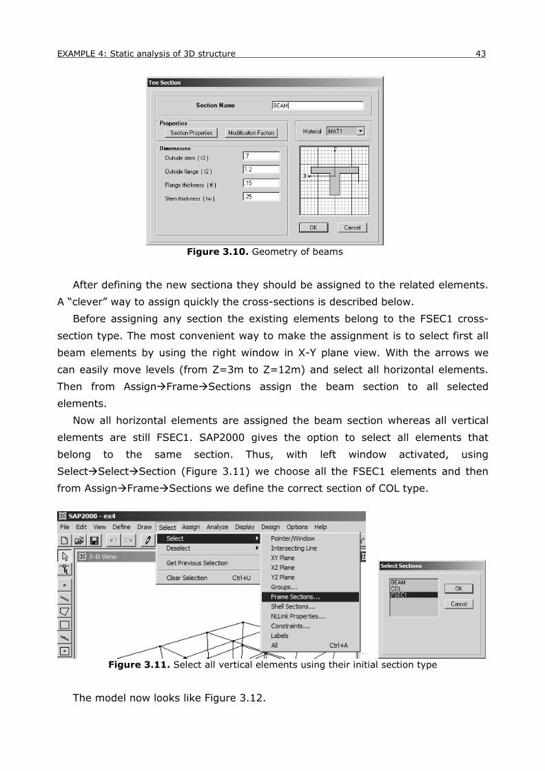
Now all horizontal elements are assigned the beam section whereas all vertical
elements are still FSEC1. SAP2000 gives the option to select all elements that
belong to the same section. Thus, with left window activated, using
SelectSelectSection (Figure 3.11) we choose all the FSEC1 elements and then
from AssignFrameSections we define the correct section of COL type.
Figure 3.11. Select all vertical elements using their initial section type
The model now looks like Figure 3.12.

EXAMPLE 4: Static analysis of 3D structure 44
Figure 3.12. 3D view of the structure
From set elements show extrusions (left window activated) we can view a
3D-visualization of the elements dimensions. This way is convenient to easily detect
any geometry errors or section assignment errors.
Figure 3.13. 3D visualization of cross-section dimensions

EXAMPLE 4: Static analysis of 3D structure 45
3.4 Loads
For this example we need to create 4 separate Static Load Cases.
- G for permanent actions
- Q for variable actions
- EX for earthquake forces in X direction
- EY for earthquake forces in Y direction
Figure 3.14. Load cases definition
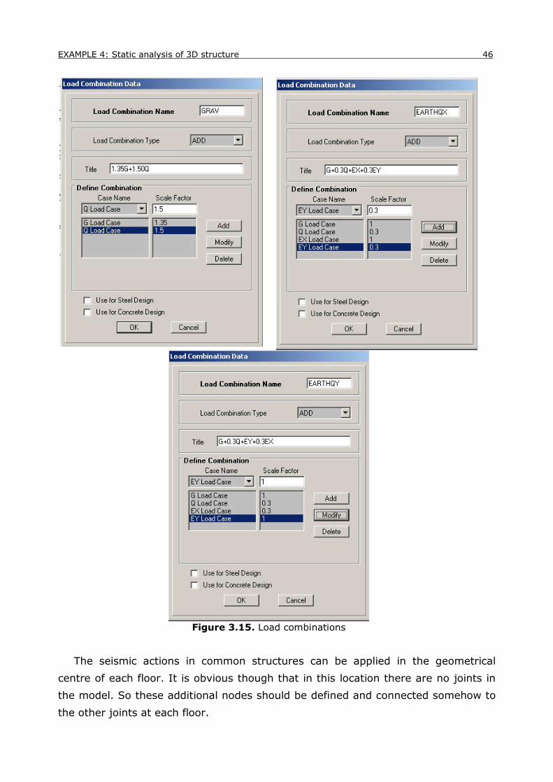
Then the appropriate load combinations according to EC-8 are defined. These
are:
- GRAV: Gravitational 1.35G+1.50Q
- EARTHQX: G+0.3Q+EX+0.3EY
- EARTHQY: G+0.3Q+EY+0.3EX
In the previous earthquake combinations we must notice that according to the
code we do not add the maximum values of EX and EY directions of the earthquake
forces. The code suggests that when the full power of the earthquake hits the
structure in X-direction, then we can accept that the simultaneous Y-direction is up
to 30% of its maximum value. Moreover, as explained in Example 2, the
simultaneous vertical loading is assumed not to exceed G+0.3Q at the moment of
the earthquake.
Load combinations are defined according to Figure 3.15.
EXAMPLE 4: Static analysis of 3D structure 46
Figure 3.15. Load combinations
The seismic actions in common structures can be applied in the geometrical
centre of each floor. It is obvious though that in this location there are no joints in
the model. So these additional nodes should be defined and connected somehow to
the other joints at each floor.

EXAMPLE 4: Static analysis of 3D structure 47
In order to make the creation of the new joints easier we define some additional
Grid Lines from Draw Edit Grid inserting value 0 in X and Y direction.
Figure 3.16. Introduction of new joints at (0,0)
After defining the new grid lines the Figure 3.17 appears..
Figure 3.17. Appearance of the new grid lines
After moving to the first floor (Z=3) of the X-Y view we can insert a new joint
using the command DrawAdd Special Joint and then clicking once at the centre of
the floor. After creating the new joint it is essential we press Escape button to avoid
accidental drawing of other joints. Right-clicking the joint can verify if the
coordinates are correct.

EXAMPLE 4: Static analysis of 3D structure 48
Figure 3.18. Drawing new joint
Now if we move to an X-Z view in the right window and using the arrows go to
Y=0 we can see the joined that was previously drawn.
We can create joints at the remaining floors by selecting the joint and go to
EditCopy. Then again from EditPaste we provide the required information for the
new joint to be created. Here we want to copy the joint from Z=3 to Z=6, Z=9 and
Z=12. In Figure 3.19 we are supposed to provide the height difference value
between the copied and the paste location. Thus the Delta Z value should be equal
to 3m, 6m and 9m.
Figure 3.19. Copy to new joints
After drawing all the new joints we specify the loads applied on them. We first
make sure that in the right window the X-Z plane is visible at level Y=0. We choose
the joint of the first floor and assign first the horizontal load in X-direction using
AssignJoint Static LoadsForces and inserting 100kN in the “Force Global X” field
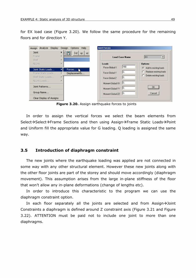
EXAMPLE 4: Static analysis of 3D structure 49
for EX load case (Figure 3.20). We follow the same procedure for the remaining
floors and for direction Y.
Figure 3.20. Assign earthquake forces to joints
In order to assign the vertical forces we select the beam elements from
SelectSelectFrame Sections and then using AssignFrame Static LoadsPoint
and Uniform fill the appropriate value for G loading. Q loading is assigned the same
way.
3.5 Introduction of diaphragm constraint
The new joints where the earthquake loading was applied are not connected in
some way with any other structural element. However these new joints along with
the other floor joints are part of the storey and should move accordingly (diaphragm
movement). This assumption arises from the large in-plane stiffness of the floor
that won’t allow any in-plane deformations (change of lengths etc).
In order to introduce this characteristic to the program we can use the
diaphragm constraint option.
In each floor separately all the joints are selected and from AssignJoint
Constraints a diaphragm is defined around Ζ constraint axis (Figure 3.21 and Figure
3.22). ATTENTION must be paid not to include one joint to more than one
diaphragms.

EXAMPLE 4: Static analysis of 3D structure 50
Figure 3.21. Diaphragm definition at floor level
Figure 3.22. Diaphragm definition at floor level
After defining the diaphragms, the nodes at the centre of each floor are
“connected” to the rest of the floor and they move along it. This way the earthquake
load applied on the joints is transferred to the structure.
3.6 Analysis
After finishing the input data
introduction and select 3D analysis
from AnalyzeSet Options we are
ready to run the analysis.
Figure 3.23. 3D analysis of the model

EXAMPLE 4: Static analysis of 3D structure 51
3.7 Results
Indicatively we can see the bending moments diagram of the corner column for the
GRAV load combination:
a) for the frame of X direction (moment Μ33 - Figure 3.24)
b) for the frame of Y direction (moment Μ22 - Figure 3.25)
Figure 3.24. Moment of the corner column (bending of X-direction frame - Μ33)
Figure 3.25. Moment of the corner column (bending of Y-direction frame – Μ22)