Equity and emissions trading in China

Supplementary Material

Da Zhanga,b, Marco Springmannc,*, Valerie Karplusb

aInstitute of Energy, Environment and Economy, Tsinghua University, Beijing, China;

bJoint Program of the Science and Policy of Global Change, Massachusetts Institute of

Technology, Cambridge, USA;

cDepartment of Economics, University of Oldenburg, Germany;

*Corresponding author: Marco Springmann, Department of Economics, University of

Oldenburg, 26111 Oldenburg, Germany. E-mail: marco.springmann@uni-oldenburg.de.

ContentsS1 Regional aggregation......................................................................................................2S2 Consumption-based emissions inventories.....................................................................3S3 Stand-alone rule and unconstraint allocation scenarios..................................................5S5 Description of the energy-economic model....................................................................8S6 Emissions reductions in the ETS allocation scenarios..................................................11S7 Permit transfers.............................................................................................................12S8 Welfare impacts by province........................................................................................14S9 Sensitivity analysis of emissions targets and elasticities of substitution......................15S10 Sensitivity analysis of mixed allocation schemes.........................................................18S11 Comparison of ETS scenarios to regional emissions-intensity targets.........................20S12 Survey details................................................................................................................22S13 Supplementary survey results.......................................................................................24S14 Respondents’ preferences by region of origin and residence........................................26Supplementary References.......................................................................................................28

1

S1 Regional aggregation

For ease of presentation, we group China’s provinces into eastern, central, and western ones

according to the three economic zones defined in China's Seventh Five-Year Plan (State

Council of China, 1986; Feng et al., 2012).1 Supplementary Figure S1 provides the details of

this regional aggregation.

Fig. S1 Overview of Chinese provinces included in the analysis2

1 Following Feng et al. (2012), we group Guangxi as a western province due to its economic similarities with western provinces. Although Inner Mongolia is sometimes also grouped as a western province, we group it as a central province, which is in line with its economic characteristics and with the grouping described by the State Council of China (1986).2 The eastern provinces include Beijing (BEJ), Fujian (FUJ), Guangdong (GUD), Hainan (HAI), Hebei (HEB), Jiangsu (JSU), Liaoning (LIA), Shandong (SHD), Shanghai (SHH), Tianjin (TAJ), and Zhejiang (ZHJ); the central provinces include Anhui (ANH), Heilongjiang (HLJ), Henan (HEN), Hunan (HUN), Hubei (HUB), Jiangxi (JXI), Jilin (JIL), Neimenggu (NMG), and Shanxi (SHX); the western provinces include Chongqing (CHQ), Gansu (GAN), Guangxi (GXI), Guizhou (GZH), Ningxia (NXA), Qinghai (QIH), Shaanxi (SHA), Sichuan (SIC), Xinjiang (XIN), and Yunnan (YUN).

2

S2 Consumption-based emissions inventories

Consumption-based emissions inventories add to production-based emissions those emissions

that are embodied in imports (erℑ), but subtract those emissions that are embodied in exports (

erEX):

erCON=er

PRD+erℑ−er

EX=erPRD+Br

1\*

MERG

EFOR

MAT

()

where Br(¿ erℑ−er

EX) denotes the balance of emissions embodied in trade (BEET) (see, e.g.,

Peters and Hertwich, 2008), also referred to as emissions transfer (Peters et al., 2011).

For obtaining the interregional emissions transfers we apply a recursive diagonalization

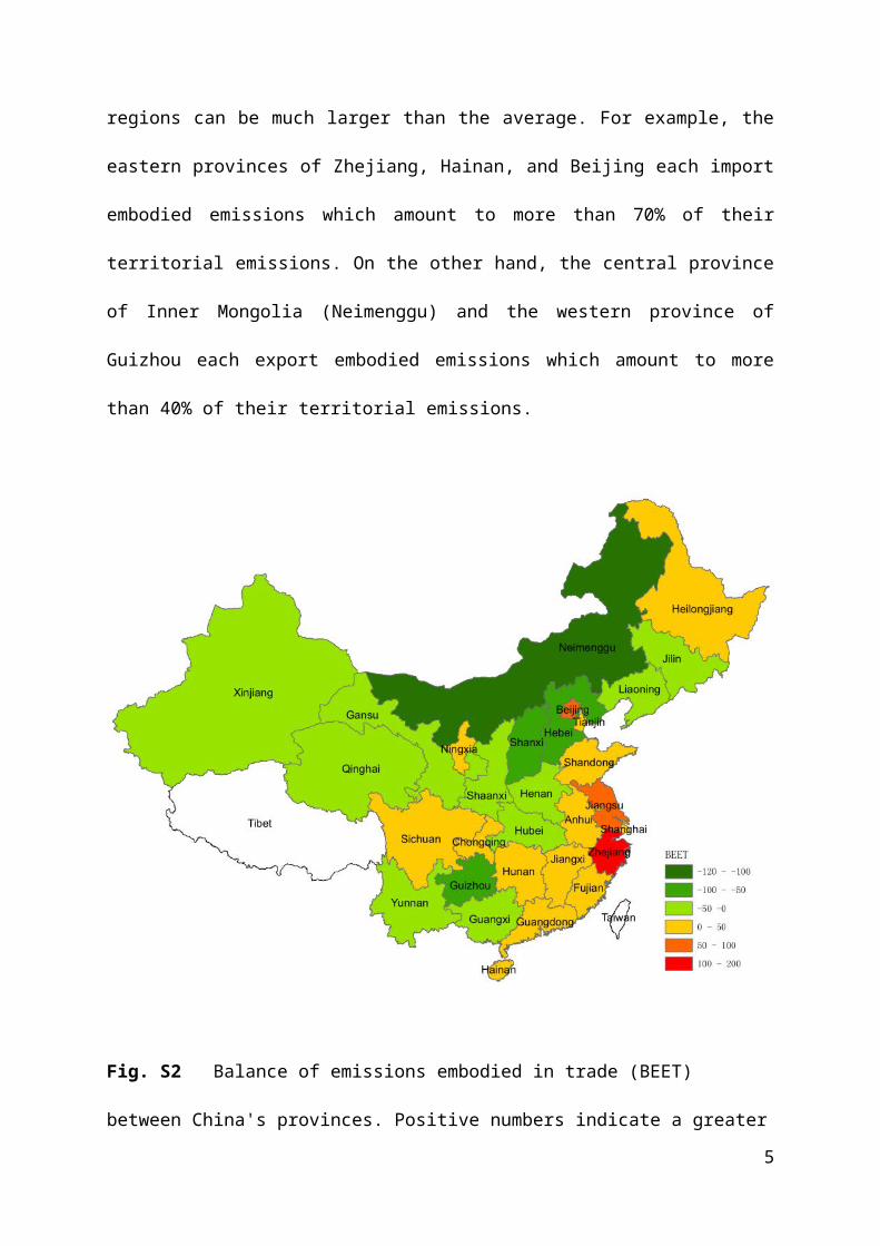
algorithm as described in Böhringer et al. (2011). Figure S2 provides an overview of China's

interregional emissions transfers (see Springmann et al., 2013 for a more detailed

description). On net, the eastern provinces import about 350 MtCO2 of embodied emissions,

i.e., 14% of their territorial emissions. Sixty percent of those emissions (212 MtCO2) are

embodied in imports from the central provinces and 40% (136 MtCO2) in imports from the

western provinces. The percentage emissions transfers for individual regions can be much

larger than the average. For example, the eastern provinces of Zhejiang, Hainan, and Beijing

each import embodied emissions which amount to more than 70% of their territorial

emissions. On the other hand, the central province of Inner Mongolia (Neimenggu) and the

3

western province of Guizhou each export embodied emissions which amount to more than

40% of their territorial emissions.

Fig. S2 Balance of emissions embodied in trade (BEET) between China's provinces.

Positive numbers indicate a greater share of emissions embodied in imports than those

embodied in exports.

4

S3 Stand-alone rule and unconstraint allocation scenarios

We constrain the permit allocation such that no province can be allocated more than its

baseline emissions. Allocated permits that would exceed the constraint are redistributed

according to each scenario's allocation factor (br

i

∑s

bsi ) with the summation indices including

the provinces among which the permits are to be redistributed. The redistribution procedure is

carried out until no province is allocated permits in excess of its baseline emissions.

Below we present the results of a sensitivity analysis which abstains from redistributing

overallocated emissions permits. Supplementary Table S3 shows that without the constraint,

the PPP, CPP, and ABT scenarios would allocate more emissions permits to the western

provinces. The analysis indicates that this overallocation would result in disproportional

wealth transfers (in terms of permit revenues) from the eastern provinces to the central and

western ones, and in significant welfare losses for the eastern provinces.

An alternative approach to avoid overallocation would be to construct aggregate allocation

scenarios as a combination of multiple allocation schemes. Supplementary Table S3 shows

that this could reduce the amount of overallocation, but it may still result in overallocation to

individual provinces if the commonly suggested combinations of allocation schemes are used.

5

Table S3 Permit allocation, permit transfers, and welfare impacts for the unconstraint

allocation scenarios and for an aggregate allocation scenario (AGG). The AGG scenario is

loosely based on an aggregate index for regional target allocation constructed by Yi et al.

(2011) which combines emissions (to indicate responsibility), inverse emissions intensities

(to indicate potential), and inverse per-capita emissions (to indicate capacity).

Allocation scenario

Permit allocation (MtCO2) Permit transfers (USD billion) Change in EV (%)Eastern Central Western Eastern Central Western Eastern Central Western

ERE 2386 1198 1075 0.85 -3.50 2.65 -0.238 -3.063 -0.629SOV 2171 1482 1007 -2.33 0.70 1.64 -0.634 -1.953 -1.024EQU 1954 1705 1000 -5.51 3.99 1.52 -1.051 -1.051 -1.051EGA 1861 1590 1208 -6.93 2.31 4.62 -1.198 -1.561 0.151PRG 1765 1805 1089 -8.31 5.47 2.84 -1.401 -0.664 -0.524PPP 1745 928 1986 -8.62 -7.46 16.09 -1.568 -4.025 4.564CPP 1315 1083 2261 -14.96 -5.17 20.13 -2.291 -3.435 6.151ESU 1035 1335 2289 -19.06 -1.40 20.46 -2.806 -2.495 6.360ABT 1014 818 2826 -19.32 -9.00 28.31 -2.910 -4.521 9.210AGG 1837 1387 1436 -7.27 -0.70 7.98 -1.258 -2.315 1.485

6

S4 Permit allocation by province

Table S4 Permit allocation (MtCO2) by province

Region ERE SOV EGA EQU PRG PPP ESU CPP ABTANH 179 147 179 149 168 179 179 179 179BEJ 108 89 68 126 85 108 108 108 92CHQ 118 97 117 127 134 118 118 118 118FUJ 148 122 148 84 86 148 148 148 148GAN 73 117 108 122 128 143 143 143 143GUD 342 281 342 202 168 179 122 178 178GXI 116 95 116 70 83 116 116 116 116GZH 79 130 156 89 100 158 158 158 158HAI 23 19 23 20 23 23 23 23 23HEB 169 294 287 277 288 172 288 228 296HEN 226 243 296 230 250 208 215 231 296HLJ 173 142 158 212 218 173 173 173 173HUB 206 170 207 93 107 207 207 207 207HUN 187 154 187 170 187 187 187 187 187JIL 137 144 113 133 140 175 175 175 175JSU 358 302 315 231 207 167 136 149 150JXI 112 92 112 86 96 112 112 112 112LIA 178 228 178 239 240 221 273 247 224NMG 113 206 100 252 251 245 250 250 219NXA 32 26 25 29 31 32 32 32 32QIH 41 69 23 65 66 83 83 83 83SHA 114 94 114 150 159 114 114 114 114SHD 277 345 388 314 311 146 176 148 208SHH 199 164 77 120 57 199 172 199 85SHX 115 183 140 381 387 222 222 222 222SIC 190 157 190 159 181 190 190 190 190TAJ 131 108 46 119 107 131 131 131 125XIN 118 97 87 129 134 118 118 118 118YUN 131 124 151 59 72 151 151 151 151ZHJ 266 219 209 220 194 231 136 139 137Eastern 2200 2171 2081 1954 1765 1727 1714 1698 1665Central 1448 1482 1491 1705 1805 1709 1721 1737 1770Western 1011 1007 1087 1000 1089 1224 1224 1224 1224

7

S5 Description of the energy-economic model

The production of energy and other goods is described by nested constant-elasticity-of-

substitution (CES) production functions which specify the input composition and substitution

possibilities between inputs (see Figure S5). Inputs into production include labor, capital,

natural resources (coal, natural gas, crude oil, and land), and intermediate inputs. For all non-

energy goods, the CES production functions are arranged in four levels. The top-level nest

combines an aggregate of capital, labor, and energy inputs (KLE) with material inputs (M);

the second-level nest combines energy inputs (E) with a value-added composite of capital and

labor inputs (VA) in the KLE-nest; the third-level nest captures the substitution possibilities

between electricity (ELE) and final-energy inputs (FE) composed, in the fourth-level nest, of

coal (COL), natural gas (GAS), gas manufacture and distribution (GDT), crude oil (CRU),

and refined oil products (OIL).

Fig S5 Nesting structure of CES production functions for non-energy goods

8

The production of energy goods is separated into fossil fuels, oil refining and gas

manufacture and distribution, and electricity production. The production of fossil fuels (COL,

GAS, CRU) combines sector-specific fossil-fuel resources with a Leontief (fixed-proportion)

aggregate of intermediate inputs, energy, and a composite of primary factors, described by a

Cobb-Douglas function of capital, and labor. Oil refining (OIL) and gas manufacture and

distribution (GDT) are described similarly to the production of other goods, but with a first-

level Cobb-Douglas nest combining the associated fossil-fuel inputs (crude oil for oil

refining; and coal, crude oil, and natural gas for gas manufacture and distribution) with

material inputs and the capital-labor-energy (KLE) nest. Electricity production is described

by a Leontief nest which combines, in fixed proportions, several generation technologies,

including nuclear, hydro, and wind power, as well as conventional power generation based on

fossil fuels. Non-fossil-fuel generation is described by a CES nest combining specific

resources and a capital-labor aggregate.

All industries are characterized by constant returns to scale and are traded in perfectly

competitive markets. Capital mobility is represented in each sector by following a putty-clay

approach in which a fraction of previously installed capital becomes non-malleable in each

sector. The rest of the capital remains mobile and can be shifted to other sectors in response

to price changes. The modeling of international trade follows the Armington (1969) approach

of differentiating goods by country of origin. Thus, goods within a sector and region are

represented as a CES aggregate of domestic goods and imported ones with associated

transport services. Goods produced within China are assumed to be closer substitutes than

goods from international sources to replicate a border effect.

9

Final consumption in each region is determined by a representative agent who maximizes

consumptions subject to its budget constraint. Consumption is represented as a CES

aggregate of non-energy goods and energy inputs and the budget constraint is determined by

factor and tax incomes with fixed investment and public expenditure.

The model is formulated as a mixed complementarity problem (MCP) (Mathiesen, 1985;

Rutherford, 1995) in which zero-profit and market-clearance conditions determine activity

levels and prices. The model uses the mathematical programming system MPSGE

(Rutherford, 1999), a subsystem of GAMS; and it is solved by using PATH (Dirkse and

Ferris, 1995).

10

S6 Emissions reductions in the ETS allocation scenarios

All national ETS scenarios result in a common cost-effective distribution of emissions

reductions. Although the absolute emissions reductions are similar for the eastern, central,

and western provinces (about 330 MtCO2 on average), the western provinces reduce

emissions the most on a percentage basis – by 27% on aggregate – followed by the central

and eastern provinces which reduce their emissions by 20% and 12%, respectively (see

Supplementary Table S6). Underlying this cost-effective distribution of emissions reductions

are regional differences in marginal abatement costs, which are highest in the eastern

provinces and lowest in the western ones – the distribution of emissions intensities is

indicative of those differences (see Figure 1 in the main text).

Table S6 Regional emissions reductions in the ETS allocation scenarios

RegionEmissions reduction

MtCO2 %

Eastern -311 -11.8%Central -366 -20.3%Western -328 -26.8%China -1005 -17.7%

11

S7 Permit transfers

Supplementary Figure S7 shows the permit (and associated financial) transfers that occur to

achieve the distribution of emissions reductions in each ETS scenario. Permit-transfer

revenues are distributed according to the difference in permits allocated to the central and

western provinces. The PPP, ESU, CPP, and ABT scenarios exhibit a roughly equal split of

permit sales between the central and western provinces, which is in line with their similarity

in absolute emissions reductions and close-to-benchmark permit allocation. In the EQU and

PRG scenarios, proportionally more permits are allocated to the central provinces than to

western ones, while proportionally more permits are allocated to the western provinces in the

ERE, SOV, and EGA scenarios. As a result, more permits are sold by the central provinces in

the EQU and PRG scenarios, and more by the western provinces in the ERE, SOV, and EGA

scenarios.

12

ERE SOV EGA EQU PRG PPP ESU CPP ABT-10

-8

-6

-4

-2

0

2

4

6

-650

-500

-350

-200

-50

100

250

Eastern Central Western

Perm

it tr

ansf

ers (

billi

on U

SD)

Perm

it tr

ansf

ers (

MtC

O2)

Fig. S7 Regional distribution of permit transfers in in billion USD (left axis) and MtCO2

(right axis)

Provincial-level transfers are listed in Supplementary Table S7.

Table S7 Value of permit transfers (USD billion) by province. Negative numbers indicate

payments and positive numbers indicate receipts.

Region ERE SOV EGA EQU PRG PPP ESU CPP ABTANH 0.430 -0.038 0.430 -0.011 0.267 0.431 0.432 0.431 0.431BEJ 0.220 -0.064 -0.383 0.487 -0.131 0.220 0.220 0.220 -0.015CHQ 0.289 -0.022 0.262 0.421 0.522 0.289 0.289 0.289 0.289FUJ 0.464 0.077 0.464 -0.477 -0.455 0.465 0.466 0.466 0.466GAN -0.257 0.401 0.266 0.470 0.563 0.773 0.774 0.774 0.774GUD 0.400 -0.498 0.399 -1.674 -2.176 -2.006 -2.858 -2.021 -2.028GXI 0.223 -0.080 0.223 -0.448 -0.254 0.224 0.224 0.224 0.224GZH -0.209 0.548 0.925 -0.064 0.103 0.965 0.965 0.965 0.966HAI 0.045 -0.015 0.045 0.003 0.040 0.045 0.045 0.045 0.045HEB -2.256 -0.414 -0.516 -0.650 -0.500 -2.215 -0.501 -1.380 -0.388HEN -0.552 -0.302 0.475 -0.496 -0.200 -0.829 -0.717 -0.477 0.477HLJ 0.347 -0.101 0.131 0.911 1.009 0.347 0.347 0.347 0.347

13

HUB 1.301 0.771 1.315 -0.366 -0.158 1.315 1.315 1.315 1.315HUN 0.635 0.144 0.635 0.381 0.632 0.634 0.635 0.634 0.635JIL 0.010 0.112 -0.348 -0.058 0.047 0.571 0.572 0.571 0.572JSU 0.357 -0.475 -0.269 -1.523 -1.876 -2.469 -2.933 -2.747 -2.732JXI 0.308 0.012 0.308 -0.089 0.073 0.308 0.308 0.308 0.308LIA -0.926 -0.187 -0.933 -0.023 -0.019 -0.292 0.477 0.082 -0.255NMG -1.308 0.069 -1.509 0.753 0.746 0.659 0.727 0.727 0.267NXA 0.079 -0.005 -0.020 0.035 0.060 0.079 0.079 0.079 0.079QIH -0.321 0.087 -0.581 0.034 0.051 0.302 0.302 0.302 0.302SHA 0.277 -0.021 0.277 0.799 0.930 0.277 0.277 0.277 0.277SHD -1.584 -0.576 0.054 -1.032 -1.081 -3.509 -3.071 -3.485 -2.600SHH 0.259 -0.263 -1.549 -0.904 -1.833 0.261 -0.132 0.261 -1.424SHX -0.984 0.031 -0.600 2.967 3.052 0.616 0.616 0.616 0.617SIC 0.244 -0.256 0.244 -0.226 0.106 0.244 0.245 0.244 0.244TAJ 0.319 -0.024 -0.941 0.146 -0.033 0.321 0.322 0.321 0.221XIN 0.507 0.199 0.051 0.674 0.746 0.506 0.507 0.506 0.507YUN 0.879 0.786 1.183 -0.177 0.014 1.184 1.183 1.183 1.183ZHJ 0.801 0.105 -0.037 0.137 -0.247 0.284 -1.117 -1.080 -1.105Eastern -1.901 -2.335 -3.666 -5.510 -8.310 -8.894 -9.081 -9.318 -9.815Central 0.188 0.699 0.836 3.992 5.469 4.052 4.236 4.474 4.970Western 1.712 1.636 2.830 1.518 2.841 4.842 4.845 4.844 4.846

S8 Welfare impacts by province

Table S8 Welfare impacts in terms of percentage changes of equivalent variation of income

by province

Region ERE SOV EGA EQU PRG PPP ESU CPP ABTANH -0.165 -1.117 -0.166 -1.051 -0.483 -0.151 -0.151 -0.156 -0.160BEJ -1.622 -2.260 -2.995 -1.051 -2.453 -1.659 -1.642 -1.654 -2.188CHQ -1.517 -2.663 -1.611 -1.051 -0.666 -1.516 -1.529 -1.523 -1.517FUJ 0.824 0.051 0.801 -1.051 -1.025 0.761 0.742 0.745 0.740GAN -5.883 -1.497 -2.388 -1.051 -0.425 0.974 0.993 0.987 0.996GUD 0.156 -0.368 0.172 -1.051 -1.331 -1.234 -1.722 -1.235 -1.231GXI 0.900 0.022 0.899 -1.051 -0.492 0.898 0.904 0.900 0.901GZH -1.726 1.647 3.309 -1.052 -0.315 3.492 3.492 3.492 3.492HAI -0.451 -1.270 -0.479 -1.051 -0.596 -0.528 -0.561 -0.550 -0.564HEB -3.721 -0.614 -0.768 -1.051 -0.788 -3.657 -0.754 -2.241 -0.563HEN -1.144 -0.794 0.266 -1.051 -0.640 -1.501 -1.341 -1.018 0.282HLJ -2.828 -4.189 -3.477 -1.051 -0.744 -2.791 -2.789 -2.789 -2.784HUB 2.121 1.116 2.143 -1.051 -0.656 2.137 2.142 2.140 2.142

14

HUN -0.580 -1.461 -0.575 -1.051 -0.596 -0.580 -0.566 -0.571 -0.569JIL -0.846 -0.574 -1.871 -1.051 -0.776 0.687 0.679 0.676 0.663JSU 0.566 -0.148 0.025 -1.051 -1.356 -1.790 -2.195 -2.039 -2.037JXI 0.239 -0.714 0.240 -1.051 -0.533 0.232 0.234 0.234 0.237LIA -2.620 -1.335 -2.633 -1.051 -1.043 -1.520 -0.183 -0.871 -1.458NMG -8.784 -3.649 -9.496 -1.050 -1.063 -1.448 -1.172 -1.181 -2.866NXA -0.203 -1.801 -2.111 -1.051 -0.605 -0.259 -0.294 -0.282 -0.295QIH -10.763 0.376 -17.887 -1.053 -0.580 6.218 6.232 6.232 6.238SHA -2.898 -3.868 -2.908 -1.051 -0.621 -2.846 -2.843 -2.849 -2.863SHD -1.507 -0.626 -0.066 -1.051 -1.104 -3.243 -2.869 -3.231 -2.451SHH 0.858 0.009 -1.943 -1.051 -2.485 0.766 0.136 0.745 -1.839SHX -16.907 -12.764 -15.327 -1.052 -0.712 -10.412 -10.392 -10.401 -10.397SIC -0.301 -1.095 -0.299 -1.051 -0.520 -0.294 -0.288 -0.290 -0.288TAJ -0.054 -1.780 -6.202 -1.050 -1.920 -0.136 -0.192 -0.173 -0.667XIN -1.954 -3.497 -4.251 -1.051 -0.681 -1.928 -1.931 -1.930 -1.926YUN 2.382 2.076 3.370 -1.051 -0.426 3.358 3.370 3.366 3.376ZHJ -0.243 -1.013 -1.149 -1.051 -1.469 -0.870 -2.338 -2.294 -2.337Eastern -0.582 -0.634 -0.788 -1.051 -1.401 -1.479 -1.496 -1.530 -1.583Central -2.102 -1.953 -1.932 -1.051 -0.664 -1.056 -1.003 -0.947 -0.824Western -1.002 -1.024 -0.574 -1.051 -0.524 0.253 0.256 0.254 0.256

S9 Sensitivity analysis of emissions targets and elasticities of substitution

We analyse the sensitivity of our results by varying key policy and model parameters. The

parameters are the overall emissions target and the elasticities governing the substitution of

energy goods with other goods and of goods produced in each province with those produced

in other provinces. Below we list the scenarios considered in the sensitivity analysis and the

welfare impacts (in terms of equivalent variation of income) associated with those. For ease

of presentation, we focus on three allocation schemes (SOV, EGA, ESU) which capture the

spread of the allocation schemes considered in this study (see Figure 3).

Stringency of the national emissions target (base case: 17.7%): 

15

- high_target: target is increased to 25%

- low_target: target is decreased to 10%

Fig. S9.1 Sensitivity analysis with respect to changes in the national emissions target.

Figure S9.1 indicates that increasing the stringency of the national emissions target increases

regional welfare impacts, while decreasing the stringency decreases them. The relative

regional distribution of welfare impacts across the different the allocation scenarios is

preserved in each case, i.e., going from the allocation scheme SOV over EGA to ESU

decreases the welfare impacts for the western provinces and increases impacts for the eastern

provinces.

Elasticity of substitution between energy input and value added (base case: 0.5):

- high_sub: 1.0

- low_sub: 0.1  

16

Fig. S9.2 Sensitivity analysis with respect to changes in the elasticity of substitution between

energy inputs and value added.

Figures S9.2 and S9.3 indicate that changing the elasticity of substitution between energy

inputs and other goods (value added) and the elasticity between goods produced with a

province and good produced in other provinces each lead to numerical changes in the

regional welfare impacts, but the relative regional distribution of welfare impacts across the

allocation schemes is preserved in each case.

Armington elasticity of substitution between goods produced within the province and

good imported from other provinces of China:

- high_trd: twice of base case Armington elasticity by sector

- low_trd: one half of base case Armington elasticity by sector

17

Fig. S9.3 Sensitivity analysis with respect to changes in the elasticity of substitution between

goods produced within each province and good imported from other provinces.

S10 Sensitivity analysis of mixed allocation schemes

In the discussion on international burden sharing, several multi-criteria schemes have been

proposed. For example, Baer et al. (2008) propose a scheme which combines capacity and

responsibility, and Raupach et al. (2014) compares a blended allocation scheme which

equally weights the idea of “inertia” and “equity”. Previous studies have adopted similar

ideas in the Chinese context with respect to sharing the national emissions reduction target

among Chinese provinces (Springmann et al., 2015; Wei et al., 2011; Yi et al., 2011).

Based on this literature, we complement our analysis by analyzing two allocation schemes

which combine different equity principles. One combines the principles of polluter pays and

18

ability to pay (PPP+ABT), and one the principles of sovereignty and egality (SOV+EGA).

The first can be seen as combining indicators of emissions responsibility (PPP) and economic

capacity (ABT) (see, e.g., Baer et al., 2008), and the second as combining indicators of inertia

with respect to emissions (SOV) and population-based equity (EGA) (Raupach et al., 2014).

Figures S10.1 and S10.2 display the permit allocation and welfare changes of the two mixed

allocation methods compared to the individual ones. The permit allocation and the welfare

changes of the mixed allocation schemes are, in each case, close to the individual allocation

schemes that are combined. Contributing to this finding is that the individual allocation

schemes that are combined (PPP and ABT, and SOV and EGA) already result in broadly

similar permit allocations and welfare impacts due to the use of the “stand-alone rule” (Lange

et al., 2007), which we adopted to avoid overallocating provinces with emissions permits

above their baseline emissions levels.

PPP ABT PPP+ABT SOV EGA SOV+EGA0

500

1000

1500

2000

2500

Eastern Central Western

Perm

it al

loca

tion

(MtC

O2)

Fig. S10.1 Regional permit allocation to China’s eastern, central, and western provinces for

selected single-criterion allocation scenarios and two multi-criteria scenarios.

19

PPP ABT PPP+ABT SOV EGA SOV+EGA-2.5

-2

-1.5

-1

-0.5

0

0.5

Eastern Central WesternCh

ange

in E

V (%

)

Fig. S10.2 Welfare impacts in terms of equivalent variation of income (%) for China’s

eastern, central, and western regions for selected single-criterion allocation scenarios and two

multi-criteria scenarios.

S11 Comparison of ETS scenarios to regional emissions-intensity targets

In order to understand how the distributional impacts compare with current policy, we

compare the menu of allocation schemes described in the main text to the regional emissions-

intensity targets of the Twelfth Five-Year Plan. The regional emissions-intensity targets of

the Twelfth Five-Year Plan are differentiated by province (see Supplementary Table S11).

However, because their regional differentiation is modest, their static emissions-reduction

equivalent as calculated is with our energy-economic model is similar to the reduction of

emissions permits with respect to benchmark emissions in the ERE, SOV, and EGA scenarios

which feature similar proportional cutbacks in emissions permits for each region.

20

Table S11 Emissions intensity targets of China's Twelfth Five-Year Plan by province

Carbon intensity reduction target (%)

Provinces

19.5 Guangdong19 Tianjin, Shanghai, Jiangsu, Zhejiang18 Beijing, Hebei, Liaoning, Shandong17.5 Fujian, Sichuan

17Shanxi, Jilin, Anhui, Jiangxi, Henan, Hubei, Hunan, Chongqing, Shannxi

16.5 Yunnan

16Neimenggu, Heilongjiang, Guangxi, Guizhou, Gansu, Ningxia

11 Hainan, Xinjiang10 Qinghai, Xizang

For further comparison to the regional emissions-intensity targets of the Twelfth Five-Year

Plan, we simulate their welfare impacts by using the energy-economic model outlined in the

section 3. Our simulations indicate that each ETS scenario increases national welfare by 30%

compared to the regional emissions-intensity targets (see also Zhang et al., 2013). Figure S11

shows the welfare impacts of the regional emissions-intensity targets and those of the

different ETS allocation scenarios by region. The figure indicates that the central and western

provinces would decrease their welfare losses in all allocation schemes when moving from

the regional target allocation of China’s Twelfth Five Year Plan to a national ETS. In

contrast, the eastern provinces would decrease their welfare losses only in the ERE, SOV,

and EGA scenarios, but their welfare decreases more in the EQU, PRG, PPP, ESU, CPP, and

ABT scenarios. The potentially negative consequences for the eastern provinces in the latter

scenarios may hinder their adoption given the political influence of those provinces.

21

ERE/SOV EGA EQU PRG PPP/ESU/CPP/ABT-2.5

-2

-1.5

-1

-0.5

0

0.5

Eastern Central WesternREG_Eastern REG_Central REG_Western

Chan

ge in

EV

(%)

Fig. S11 Welfare impacts in terms of equivalent variation of income (%) for China’s

eastern, central, and western regions in the different allocation scenarios. The dashed

horizontal lines indicate the welfare changes associated with the regional emissions-intensity

targets of the Twelfth Five-Year Plan (expressed as static emissions-reduction equivalents).

S12 Survey details

The survey was distributed at two instances in June and July 2013 in China. The first instance

was a CGE modeling workshop organized by the Center for Energy Economic and Strategy

Studies (CEESS) of Fudan University, held on June 14-15, 2013, in Shanghai. The second

was the Annual Stakeholders Meeting of the Tsinghua-MIT China Energy and Climate

Project (CECP), held on June 18, 2013, in Beijing. Supplementary Table S12.1 contains a list

of the institutional affiliations of the participating researchers. Before distributing the survey,

we conducted two target-group assessments at an ETS workshop organized by the European

Commission DG Climate Action in Beijing on May 22, 2013, and at the Environment and

22

Energy Track of the Shanghai Forum, which took place on May 25-27, 2013, in Shanghai.

Based on those assessments, we are comfortable with the representation of relevant research

teams in our focus group.

We received 44 responses. However, not all participants answered all questions, and as a

result the number of responses differs across the questions. Supplementary Table S12.2 lists

the participants’ characteristics. Almost all respondents (41 out of 44; 93%) declare

themselves as academics and about half of the respondents are below 30 years of age.

Although three-fourths of the respondents now live in eastern China (77%), more than half of

the respondents were born in central and western China (43% and 11%, respectively).

Table S12.1 Institutional affiliations of target group members

Affiliations of target group membersBeijing Institute of TechnologyBeijing Normal UniversityChinese Academy of SciencesChinese Academy of Social SciencesChina Agricultural UniversityChina Guodian Energy Research InstituteChina University of PetroleumChongqing Technology and Business UniversityDevelopment Research Center of the State CouncilEnergy Research Institute of the NDRCFudan UniversityGuangzhou Institute of Energy ConversionHunan UniversityRenmin University of China

23

Shanghai Academy of Social SciencesShanghai Environment and Energy ExchangeState Information CenterTianjin University of Science and TechnologyTsinghua UniversityWuhan University

Table S12.2 Description of survey participants

Participants' characteristics Frequency Percent

AffiliationAcademic 41 93.18Government 1 2.27Other 2 4.55

AgeBelow 30 23 52.2730 or above 14 31.82No information 7 15.91

GenderFemale 17 59.09Male 26 38.64No information 1 2.27

Origin

East 19 43.18Center 19 43.18West 5 11.36No information 1 2.27

Residence

East 34 77.27Center 8 18.18West 1 2.27No information 1 2.27

S13 Supplementary survey results

Table S13 Survey questions related to equity concerns and the trade-off between equity and

efficiency.

Participants' attitudes towards equity Frequency Percent

How concerned you are with the way the economic burden of greenhouse gas reduction is distributed among China’s provinces?

   

Very concerned 24 54.55 Somewhat concerned 12 27.27 Neutral 6 13.64 Not very concerned 2 4.55 Not concerned at all 0 0

24

What is most important for you: a fair distribution of emissions reduction burden (equity), reducing emissions at least cost (efficiency), or both?

   

Both are equally important. 24 54.55 Reducing emissions at least cost is more important. 12 27.27 A fair distribution of reduction burden is more important. 8 18.18

Fig. S13 Respondents’ agreement with the individual allocation schemes summarized in the

PPP/ESU/CPP/ABT group

25

S14 Respondents’ preferences by region of origin and residence

Given the highly differentiated impacts of the different allocation scenarios on China’s

regions, one could expect that the respondents’ preferences are influenced by their region of

origin or their residence.3 However, our analysis (see Tables S14.1 and S14.2) does not

provide strong support for that expectation. Although we find that most respondents living in

central provinces prefer the PRG scenario which puts least burden on their provinces, a

higher number of respondents living in the eastern provinces prefers the PPP/CPP/ABT/ESU

scenario which puts the greatest burden on the eastern provinces. Reasons for the small effect

of regional association may be the selection of respondents and the structure of

environmental governance in China. Our target group was comprised of experts which

provide regular input into the policy-making process. Traditionally, environmental (including

climate) policy issues are often addressed at the central level in China, and balancing impacts

across regions is often an important consideration. Thus, the experts in our target group may

adopt a regionally more balanced view on distributional and efficiency issues than lay

persons or representatives from affected industries.

3 By “residence” we are referring to physical residence, not registered (hukou) residence.

26

Table S14.1 Respondents’ final preference for the different ETS allocation scenarios

differentiated by region of origin

Final preferenceRegion of origin

TotalEast Center West No information

SOV/ERE 1 1 2 0 4EGA 2 1 0 0 3EQU 2 3 0 0 5PRG 6 6 0 1 13PPP/CPP/ABT/ESU 8 8 3 0 19Total 19 19 5 1 44

Table S14.2 Respondents’ final preference for the different ETS allocation scenarios

differentiated by region of residence

Final preferenceRegion of residence

TotalEast Center West No information

SOV/ERE 3 1 0 0 4EGA 2 1 0 0 3EQU 4 1 0 0 5PRG 8 4 0 1 13PPP/CPP/ABT/ESU 17 1 1 0 19Total 34 8 1 1 44

27

Supplementary References

Armington PS (1969) A Theory of Demand for Products Distinguished by Place of

Production. International Monetary Fund Staff Papers 16(1):159-176

Baer P, Fieldman G, Athanasiou T, Kartha S (2008) Greenhouse Development Rights:

towards an equitable framework for global climate policy. Camb Rev Int Aff 21: 649–

669.

Böhringer C, Carbone JC, Rutherford TF (2011) Embodied carbon tariffs. NBER Working

Paper No. 17376, National Bureau of Economic Research, Cambridge, MA

Dirkse SP, Ferris MC (1995) The PATH Solver: a non-monontone stabilization scheme for

Mixed Complementarity Problems. Optim Method Softw 5:123–156

Mathiesen L (1985) Computation of economic equilibria by a sequence of linear

complementarity problems. Math Program Stud 23:144–162

Peters GP, Minx JC, Weber CL, Edenhofer O (2011) Growth in emission transfers via

international trade from 1990 to 2008. PNAS 108(21):8903–8908

Peters GP, Hertwich EG (2008) CO2 embodied in international trade with implications for

global climate policy. Environ Sci Technol 42(5):1401–1407

Raupach MR et al. (2014) Sharing a quota on cumulative carbon emissions. Nat Clim Change

4: 873–879.

Rutherford TF (1995) Extension of GAMS for complementarity problems arising in applied

economic analysis. J Econ Dyn Control 19(8):1299–1324

Rutherford TF (1999) Applied general equilibrium modeling with MPSGE as a GAMS

subsystem: an overview of the modeling framework and syntax. Comput Econ 14:1–46

28

Springmann M, Zhang D, Karplus VJ (2015) Consumption-Based Adjustment of Emissions-

Intensity Targets: An Economic Analysis for China’s Provinces. Environ Res Econ 61:

615–640

Wei C, Ni J, Du L (2011). Regional allocation of carbon dioxide abatement in China. China

Econ Rev 23(3):552-565

Yi WJ, Zou LL, Guo J, Wang K, Wei YM (2011) How can China reach its CO2 intensity

reduction targets by 2020? A regional allocation based on equity and development.

Energ Policy 39(5):2407–2415

Zhang D, Rausch S, Karplus V, Zhang X (2013) Quantifying Regional Economic

Impacts of CO2 Intensity Targets in China. Ener Econ 40: 687–701

29