Standard back-propagation artificial neural networks for cloud liquid water path retrieval from AMSU-B data

John M. Palmer, Filomena Romano, Domenico Cimini, Vincenzo Cuomo. Institute of Methodologies for Environmental Analysis, National Council Research,

Potenza, Italy.

Abstract Artificial neural networks (ANNs) have many variants, which can have very different behaviours. The success of ANNs to produce good results for a wide variety of problems when little is known about the search space has lead them to become of interest to many scientific disciplines. Ideally if a problem is tested for the first time with an ANN methodology then this methodology should be standard. However this may be problematic for a number of reasons. It is difficult to know the best configuration of parameters for the learning algorithm. Results from individual runs can be irregular. There may be a very large amount of training data making training slow. These problems often cause researches to diverge from the standard back propagation method. The objective of this study is to test ANN methodology for the problem of cloud liquid water path (LWPC) derivation, using the advanced microwave sounding unit B (AMSU-B) microwave brightness temperatures. The vertically integrated cloud liquid water, also known as LWPC plays a key role in the study of global atmospheric water circulation and the evolution of clouds. The ability to derive LWPC accurately and across large areas therefore means better atmospheric models can be built and tested. Simulated AMSU-B and LWPC data is fitted using linear, polynomial and standard ANN methods. The ANN method performed the best and gave an average RMS error for between 0.06 and 0.02 kgm-2 dependent on the environment.

Introduction Retrieving the cloud liquid water path (LWPC) from satellite brightness temperatures is an example of the inverse problem. The attraction to the use of ANNs in the wider sciences is their resilience to noise or missing data, they can be highly non-linear and provide a tool to fit a function to data where the data is little understood. Because of this ANNs are often used to find solutions inverse problems. Artificial neural networks The term ‘artificial neural network’ is more historical than descriptive and in fact refers to the original inspiration for their development [6]. An ANN is a multivariable function in continuous space. It is more concisely depicted graphically but each output can also be written as a function of the ANN inputs. Changing the free parameters of an ANN changes the function it produces. ANN free parameters are called biases and weights. A standard feed forward artificial neural network is shown in figure 1, and has 3 layers. The inputs biases and weights are labelled. Each unit outputs a function of its inputs. This function is called the activation function. Selecting values for the biases and weights is done to fit the entire ANN function to data.

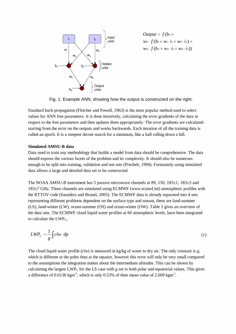
Fig. 1: Example ANN, showing how the output is constructed on the right. Standard back-propagation (Fletcher and Powell, 1963) is the most popular method used to select values for ANN free parameters. It is done iteratively, calculating the error gradients of the data in respect to the free parameters and then updates them appropriately. The error gradients are calculated starting from the error on the outputs and works backwards. Each iteration of all the training data is called an epoch. It is a steepest decent search for a minimum, like a ball rolling down a hill. Simulated AMSU-B data Data used to train any methodology that builds a model from data should be comprehensive. The data should express the various facets of the problem and its complexity. It should also be numerous enough to be split into training, validation and test sets (Prechelt, 1994). Fortunately using simulated data allows a large and detailed data set to be constructed. The NOAA AMSU-B instrument has 5 passive microwave channels at 89, 150, 183±1, 183±3 and 183±7 GHz. These channels are simulated using ECMWF (www.ecmwf.int) atmospheric profiles with the RTTOV code (Saunders and Brunel, 2005). The ECMWF data is already separated into 4 sets representing different problems dependent on the surface type and season, these are land-summer (LS), land-winter (LW), ocean-summer (OS) and ocean-winter (OW). Table 1 gives an overview of the data sets. The ECMWF cloud liquid water profiles at 60 atmospheric levels, have been integrated to calculate the LWPC,

∫ ⋅= dpclwg

LWPC

1 (1)

The cloud liquid water profile (clw) is measured in kg/kg of water to dry air. The only constant is g, which is different at the poles than at the equator, however this error will only be very small compared to the assumptions the integration makes about the intermediate altitudes. This can be shown by calculating the largest LWPC for the LS case with g set to both polar and equatorial values. This gives a difference of 0.0138 kgm-2, which is only 0.53% of their mean value of 2.609 kgm-2.

))(

)(

(

241226

231115

3

iwiwbfw

iwiwbfw

bfOutput

⋅+⋅+⋅

+⋅+⋅+⋅

+=

Table 1: An overview of the LWPC data. Note that the mode is the most frequent value after rounding to 2 decimal places. Case Temporal range Spatial range

(Latitude) Number of profiles

Mode LWPC

Mean LWPC

Range of LWPC

Land-summer Land-winter Ocean-summer Ocean-winter

1 to 13 Jan 2004 1 to 19 Jan 2004 14 to 26 July 2004 1 to 13 Jan 2004

-29.7 to 19.8 35.3 to 59.9 10.0 to 59.9 10.0 to 59.9

25384 5029 9006 9310

0.09 0.05 0.09 0.01

0.286 0.123 0.385 0.187

≈0 to 2.611 ≈0 to 0.835 0.005 to 2.286 ≈0 to 1.494

In this study, all 5 AMSU-B channels are used as continuous ANN inputs. No combinations or functions of these channels are considered. This is left for a further study of the data.

Methodology The configurations of the ANNs are described in the beginning of the results section, and the standard feed-forward ANN running with back propagation is well documented (Haykin, 1998), (Russell and Norvig, 1995). An important point to note about the use of ANNs that internally data is scaled differently to the final results; this is also discussed. Additionally this study makes use of a parameterised activation function a simple variation on back-propagation and a sampling technique for the input data. It is also recommended that any additional ANN methodology be tested against benchmark problems from the ANN literature; an example of this is given in this section. Data scaling for input and output representations Scaling data is important for the good working of an ANN. Most importunately the desired output representation should be producible by the networks output units. It is customary to scale real continuous input data to fit in the range 0 to 1 or –1 to 1, but this is not necessarily the better way (Haykin, 1998). It is advisable to consider any transform of an input channel as a new (optional) input channel because transforming the input data space equivalently transforms the search space, which are different. The input channels chosen for the neural network can then be considered to be taken from the set of possible channel transformations and combinations. For the problems presented in this paper only linear transformations of both input and output data are considered, where, ANN data = a (Real data) + b (2)

Error functions Throughout this study the error function employed is the same as described by Prechelt (1994), this is a squared error percentage measure: -

( )∑ ∑= =

−=

P

p

N

ipipi

Range toNP

OE

1

2

1

100 (3)

P represents the number of training examples and the equivalent summation is for all the training data. N represents the number of output nodes in the network and again the error is summed for each node. (o - t) is the network output minus the truth data. ORange is the range of the output problem

representation. This range is not necessarily the range producible by the ANN output units or the range in the scaled truth data as used with the ANN - it is the range of the distribution that the scaled truth data is considered to be selected from. In the case of this study for the simulated meteorological data it is simply taken to be the scaled range of the truth data. The truth data is typically scaled to have the range of the output unit, which for the hyperbolic tangent activation function is 2, therefore in this case ORange=2. For the LWPC retrieval there is only one output node so N=1. The error measure becomes,

( )∑=

−=

P

ppp to

PE

1

2200 (4)

For the case of the PROBEN1 benchmark problems (Prechelt, 1994), ORange is taken to be 1 and there may be more than one output unit depending on the problem. It is important to notice that researches in other scientific fields will require an error measure, such as a RMS error with the units equivalent to the measured quantity. This would be done by rescaling the output data into the original units and then making an error measure. However from equation (4) for LWPC retrieval, a conversion can be made directly,

2200a

ERMS = (5)

The term a is the scale value as used for the ANN output in equation (2). This highlights the difference between the error measures because the error used in training is globally representative of the data such that it takes into account of the range of the problem representation. When quoting the ANN error, E is taken to be unit less and so no units are given.

Parameterised activation function Considering the ANN as a regression, then the activation functions are the functions used to fit the training data. For the networks used in this study it is possible to select a different type of activation function for each hidden or output layer of the network. Sigmoid type functions are typically used (Haykin, 1998) because of the way ANN’s update their weights. Both the distribution of the training data and the functionality of the ANN would be best considered for the choice of activation function. The distribution of the LWPC and the input brightness temperatures are uneven, and in fact are more similar to log-normal than normal distributions. A parameterised activation function has been constructed with tuneable parameters, which allows for a varied set of activation functions to be tested and easily specified.

( ) ( ){ }21 tanhtanh2

vubxvbxa

y +++= (6)

With the differential (this is needed to calculate the error gradients),

( ) ( ){ }22

12 tanhtanh1

2vubxuvbxu

ab

dx

dy+−+−+= (7)

Where a and b control the scaling of the function in x and y and would be normally set to 1. The values of v1, v2 and u control how the two hyperbolic tan functions are composed. For our problem to derive LWPC, an uneven variant is chosen, similar to the standard tanh function but changing much more sharply on one side. This configuration and other examples are shown in figure 2.

Fig. 2: Some possibilities using the parameterised activation function.

Sampling training and validation data Back-propagation is slow, particularly when there is a large amount of training data. Sampling training and validation data sets is done to reduce their size. This can be done because the form of the data is more important than just the quantity. Within this study a simple method has been implemented to simple data sets. Each dimension of the data is split into S parts, for d dimensions, this makes Sd subspaces. Various statistical measures can then be used to select n points from each of the subspaces. The plots in figure 3, give a simple example of this.

Fig. 3: One point is taken at random from each of the subspaces considering only 2 dimensions of the simulated LS data set. Plot a) shows all 25384 data points b) S=200 and so 8457 points are selected, c) S=100, selecting 3755 points, d) S=25 selecting 398 points.

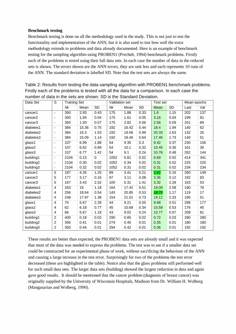
Benchmark testing Benchmark testing is done on all the methodology used in the study. This is not just to test the functionality and implementation of the ANN, but it is also used to test how well the extra methodology extends to problems and data already documented. Here is an example of benchmark testing for the sampling algorithm using PROBEN1 (Prechelt, 1994) benchmark problems. Firstly each of the problems is tested using their full data sets. In each case the number of data in the reduced sets is shown. The errors shown are the ANN errors, they are unit less and each represents 10 runs of the ANN. The standard deviation is labelled SD. Note that the test sets are always the same.

Table 2: Results from testing the data sampling algorithm with PROBEN1 benchmark problems. Firstly each of the problems is tested with all the data for a comparison. In each case the number of data in the sets are shown. SD is the Standard Deviation.

Training Set Validation set Test set Mean epochs Data Set S № Mean SD № Mean SD Mean SD Last Val

cancer1 cancer2 cancer3

- - -

350 350 350

2.93 1.94 1.50

0.43 0.04 0.07

175 175 175

1.88 1.61 2.82

0.33 0.05 0.06

1.6 3.16 2.56

1.15 0.04 0.09

202 199 201

137 81 89

diabetes1 diabetes2 diabetes3

- - -

384 384 384

15.36 16.3 15.09

0.75 1.53 1.14

192 192 192

16.42 19.06 18.46

0.44 0.99 0.64

18.4 20.33 17.46

1.94 2.63 1.73

140 132 140

62 25 51

glass1 glass2 glass3

- - -

107 107 107

6.99 6.62 6.77

1.88 0.89 1.42

54 54 54

9.35 10.1 9.1

0.3 0.32 0.24

9.42 10.45 10.76

0.37 0.35 0.48

230 161 262

106 36 144

building1 building2 building3

- - -

2104 2104 2104

0.13 0.30 0.32

0 0.02 0.02

1052 1052 1052

0.81 0.34 0.31

0.02 0.02 0.02

0.69 0.31 0.31

0.02 0.02 0.02

414 225 234

341 225 234

cancer1 cancer2 cancer3

5 5 5

187 177 167

4.26 3.17 3.43

1.25 0.16 2.52

89 97 100

3.41 3.11 5.31

0.21 0.08 1.41

1.42 3.36 3.32

0.16 0.12 2.28

260 192 163

149 83 53

diabetes1 diabetes2 diabetes3

4 4 4

263 256 248

19 18.64 17.97

1.18 0.54 1.38

164 143 154

17.42 20.85 21.01

0.51 0.53 0.73

19.09 18.79 19.12

2.58 1.17 2.33

190 119 195

78 17 51

glass1 glass2 glass3

4 4 4

70 62 66

5.67 6.18 5.67

2.28 0.77 1.18

44 45 43

9.21 10.69 9.02

0.55 0.34 0.24

9.68 10.59 10.77

0.51 0.53 0.57

298 176 208

177 45 81

building1 building2 building3

2 2 2

400 356 350

0.18 0.41 0.44

0.02 0.01 0.01

290 274 294

0.85 0.45 0.42

0.02 0.01 0.01

0.72 0.35 0.36

0.03 0.01 0.01

280 180 192

280 180 192

These results are better than expected, the PROBEN1 data sets are already small and it was expected that most of the data was needed to express the problems. The test was to see if a smaller data set could be constructed for an experimental phase of work, without sacrificing the behaviour of the ANN and causing a large increase in the test error. Surprisingly for two of the problems the test error decreased (these are highlighted in the table). Notice also that the glass problems still performed well for such small data sets. The larger data sets (building) showed the largest reduction in data and again gave good results. It should be mentioned that the cancer problem (diagnosis of breast cancer) was originally supplied by the University of Wisconsin Hospitals, Madison from Dr. William H. Wolberg (Mangasarian and Wolberg, 1990).

ANN Results and method comparison ANNs have many parameters to configure. The configurations as described below were used as the default. All networks are configured with initial weights selected randomly from the range –0.25 to 0.25. All networks are fully connected and feed forward but with no shortcut connections. The training is done using the DBProp algorithm configured with ε1=0.5, α1=0.9, ε2=0.9 and α2=0.9. Each run is terminated when either,

• The training error does not change by more than 0.1% per epoch for 100 epochs,

• The validation error is grater than 101% of the smallest validation error for a count of 100 epochs, (if the error is reducing but still above the smallest validation error, the count slows to 1 count every 2 epochs.

• 1000 epochs are reached. Standard back propagation in batch mode is configured with ε=0.7 and α=0.9. All quoted errors are the ANN error measure. The training error represents the best error on the training set at any point during training. The validation error represents the best error on the validation set at any point during training. The test error represents the error on the test set when the network is configured to the state of best validation error. The last epoch reached before the training was terminated and the epoch at the point of best validation error may also be shown in the results. The training, validation and test sets are selected randomly for each run with the proportions 50%, 25% and 25% respectively. The training and validation sets are then further reduced using the sampling algorithm with S=4. This algorithm is set to select examples that are the points closest to the mean of each of the subspaces. The input channels are scaled such that their standard deviation goes from –1 to 1 with the mean set to 0. The output channel is scaled to fit within the range –1 to 1 with the median set to 0. All channels are scaled linearly and the scaling coefficients (equation 2) are shown in table 3. Table 3: The input and output linear scaling coefficients used for the meteorological data for each of the 4 cases of surface type and season. See equation 2.

AMSU-B Input channels Output

1 2 3 4 5 LWPC a 0.1563 0.2090 0.2618 0.3220 0.3586 0.4154 LS b -43.1410 -58.4339 -64.0032 -83.1099 -96.4927 -0.0846 a 0.1578 0.1721 0.3048 0.4083 0.4067 1.3576 LW b -39.5568 -44.8334 -74.1742 -103.8742 -106.9604 -0.1330 a 0.0676 0.1408 0.3242 0.3707 0.3343 0.4939 OS b -17.2593 -38.7282 -78.8010 -95.0407 -89.4345 -0.1291 a 0.0460 0.0564 0.2440 0.3112 0.2683 0.7182 OW b -10.4627 -14.4899 -59.7382 -79.6386 -71.1445 -0.0730

The ANN architecture used was 5-20-5-1 for all networks, this notation references the number of units in each layer from input to output. Throughout the study various configurations of the ANN are tested, table 4 shows a sample of tests for the activation function.

Table 4: Results of testing a non-standard activation function for the LWPC problem. Equation (6) is used to construct this activation function, with the parameters a=1, b=1, v1=0.5, v2=-0.5 and u=3. It is referenced here, tanhC. SD is the Standard Deviation.

Training Set Validation set Test set Mean epochs Data Set

Activation Function Architecture

Mean SD Mean SD Mean SD Last Val LS LW OS OW

None-tanh-tanh-tanh None-tanh-tanh-tanh None-tanh-tanh-tanh None-tanh-tanh-tanh

0.204 0.195 0.1 0.083

0.017 0.066 0.016 0.015

0.277 0.34 0.147 0.078

0.056 0.098 0.029 0.017

0.148 0.263 0.148 0.057

0.014 0.052 0.015 0.008

690 863 733 659

690 863 716 659

LS LW OS OW

None-tanhC-tanh-tanh None-tanhC-tanh-tanh None-tanhC-tanh-tanh None-tanhC-tanh-tanh

0.182 0.139 0.086 0.059

0.035 0.024 0.021 0.012

0.219 0.319 0.143 0.077

0.053 0.054 0.036 0.016

0.155 0.327 0.135 0.052

0.024 0.08 0.023 0.005

648 1081 669 688

627 963 659 688

LS LW OS OW

None-tanhC-tanhC-tanh None-tanhC-tanhC-tanh None-tanhC-tanhC-tanh None-tanhC-tanhC-tanh

0.154 0.131 0.076 0.043

0.016 0.04 0.021 0.009

0.219 0.34 0.136 0.061

0.036 0.075 0.035 0.01

0.135 0.314 0.132 0.045

0.015 0.058 0.016 0.006

587 1003 572 733

548 881 526 711

The best of these results are selected and the RMS error in terms of kgm-2 is shown in table 5.

Table 5: The best selection of Activation Function Architecture taken from Table 4 and displayed with the test set errors in kgm-2.

Test set error (kgm-2) Data Set Activation Function Architecture Mean SD

LS LW OS OW

None-tanhC-tanhC-tanh None-tanh-tanh-tanh None-tanhC-tanhC-tanh None-tanhC-tanhC-tanh

0.062 0.027 0.052 0.021

0.004 0.002 0.003 0.001

Errors and plots of typical runs for these networks (table 5) are shown in figure 4. Notice that these are test set errors. The test set is only used once to create the test errors and has no influence on the training or selection of the final network.

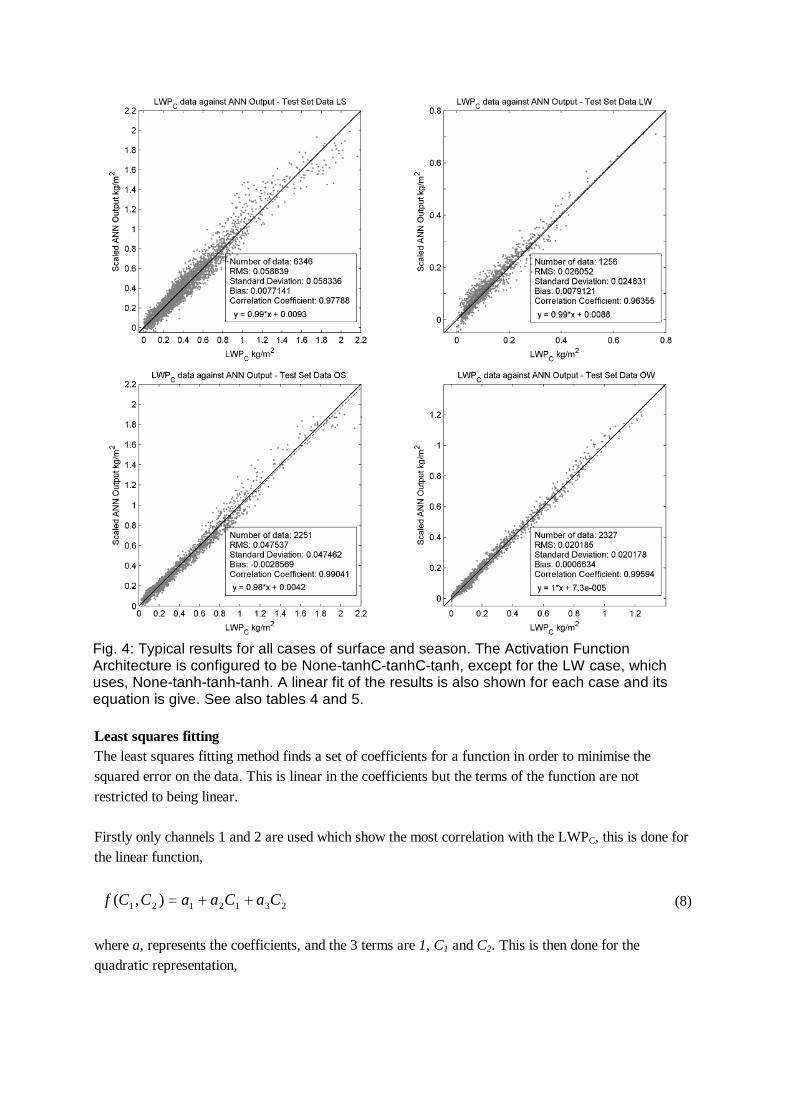
Fig. 4: Typical results for all cases of surface and season. The Activation Function Architecture is configured to be None-tanhC-tanhC-tanh, except for the LW case, which uses, None-tanh-tanh-tanh. A linear fit of the results is also shown for each case and its equation is give. See also tables 4 and 5. Least squares fitting The least squares fitting method finds a set of coefficients for a function in order to minimise the squared error on the data. This is linear in the coefficients but the terms of the function are not restricted to being linear. Firstly only channels 1 and 2 are used which show the most correlation with the LWPC, this is done for the linear function,

2312121 ),( CaCaaCCf ++= (8)

where a, represents the coefficients, and the 3 terms are 1, C1 and C2. This is then done for the quadratic representation,

( )22312121 ),( CbCbbCCf ++= (9)

When this expression is expanded there are 6 terms. Notice that in this notation, the coefficients b, inside the brackets are not the same as the coefficients a, for the expanded terms which are fitted with the least squares method. Using all the channels, both the linear and quadratic models are fitted,

5645342312154321 ),,,,( CaCaCaCaCaaCCCCCf +++++= (10)

( )25645342312154321 ),,,,( CbCbCbCbCbbCCCCCf +++++= (11)

For the quadratic with 5 channels there will be 21 terms and so 21 a coefficients. The coefficients are calculated as a vector,

( ) cTT lwpKKKa

1−= (12)

Where K is a matrix of the terms calculated from the training data and lwpc is the equivalent vector of the LWPC. 100 runs are made for each case of surface and season and for each type of fit. For each run a training and test set are randomly selected and are 50% and 25% of the data (as for the ANN model) – there is no validation set. The 4 variations of the least squares solution are labelled Linear2, Linear5, Quadratic2 and Quadratic5 dependent on the number of channels and the terms, see table 6.

Table 6: results from 100 runs of the 4 variations of the least squares solution for each case of surface and season.

Linear2 Linear5 Quadratic2 Quadratic5 Data Set Mean SD Mean SD Mean SD Mean SD LS LW OS OW

0.156 0.044 0.156 0.061

0.003 0.001 0.005 0.002

0.139 0.041 0.134 0.050

0.003 0.001 0.004 0.001

0.113 0.040 0.099 0.028

0.002 0.001 0.003 0.0008

0.071 0.029 0.072 0.025

0.002 0.001 0.003 0.0005

Using all 5 channels with the quadratic model did the best, again typical results are plotted for all cases of surface and season, figure 5.

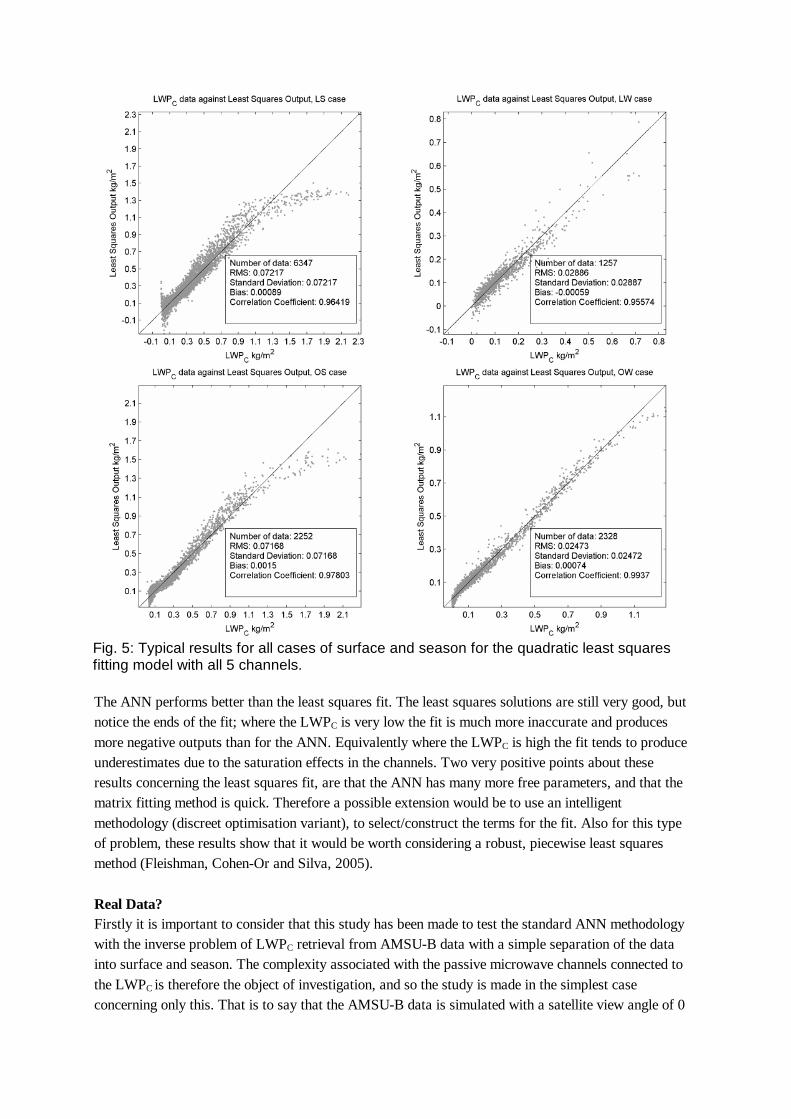
Fig. 5: Typical results for all cases of surface and season for the quadratic least squares fitting model with all 5 channels. The ANN performs better than the least squares fit. The least squares solutions are still very good, but notice the ends of the fit; where the LWPC is very low the fit is much more inaccurate and produces more negative outputs than for the ANN. Equivalently where the LWPC is high the fit tends to produce underestimates due to the saturation effects in the channels. Two very positive points about these results concerning the least squares fit, are that the ANN has many more free parameters, and that the matrix fitting method is quick. Therefore a possible extension would be to use an intelligent methodology (discreet optimisation variant), to select/construct the terms for the fit. Also for this type of problem, these results show that it would be worth considering a robust, piecewise least squares method (Fleishman, Cohen-Or and Silva, 2005).

Real Data? Firstly it is important to consider that this study has been made to test the standard ANN methodology with the inverse problem of LWPC retrieval from AMSU-B data with a simple separation of the data into surface and season. The complexity associated with the passive microwave channels connected to the LWPC is therefore the object of investigation, and so the study is made in the simplest case concerning only this. That is to say that the AMSU-B data is simulated with a satellite view angle of 0

and with the surface emissivity left as the default by the RTTOV code (Saunders and Brunel, 2005). Additionally no extra consideration such as latitude was used as input into the neural network. It is true then that this does not fully represent the real situation, however it is also true that for a real operation algorithm, you would not expect one single heuristic to solve the global problem. Adding extra information into the study is therefore considered an extension particularly when the extra data is known before the retrieval. So can an ANN trained with simulated data be tested with real data? Consider the following general argument,

• Mechanism A is used to create the data set, data A and we want to use this data to learn a model for mechanism A. We first split the data into Training set A, Validation set A and Test set A.

• Now consider a second mechanism B, which creates data B. If mechanisms A and B are in fact the same, then data A and data B can be considered as parts of a bigger data set, we will call data C.

• If a model is trained with Training set A, and validated with Validation set A such that the best trained state of the model can be selected, then testing the model with any other part of data C, would be equivalent…

• Unless, a) Data C is not evenly mixed. b) Mechanisms A and B are NOT the same.

From the argument above,

( ) )()()()( xDataCxSetAValidationxATraininSetxetValidTestSx ∧∨¬→∀ (13)

And so the question should be, what is being tested when real data is used with an ANN trained with simulated data? A set of real data has been constructed by co-locating data from the NOAA CLASS web site (www.class.noaa.gov) with ground station data from the ARM web site (www.arm.gov). A range of LWPC has been selected from the Southern Great Plains stations Central and Hillsboro. In total the final data set contains 99 data points. However this data set is not complete enough to learn a model to represent the mechanism that created it. Some simple tests have been made to demonstrate this. ● Test of comprehensive data 1: The convex hull test The convex hull of a data set the tessellating boundary described by the data set. The data set is first randomly split into 2 equally sized subsets, a and b. Both these parts should represent (comprehensively) the same function and so should be similar. The test is to see what fraction of subset b lays within the convex hull of a. This test is run 50 times for both the real data and the simulated data (LW case). The test is done using the 5 dimensions of the brightness temperatures. The simulated data mean result is 92% with a standard deviation of 0.6%. Compare this to real data mean result of 37% with a standard deviation of 8%. In higher dimensional space the complex hull needs more points to describe it (Landgrebe, 1997). Having fewer points is less of a problem if the shape in the high dimensional space is simple.

● Test of comprehensive data 2: The closest point test Again the data set is first randomly split into 2 equally sized subsets, a and b. The test is a measure of the mean distance for each point in subset b to the closest point in subset a. This is also run 50 times for both the real data and the simulated data (LW case). The test is done using the 5 dimensions of the brightness temperatures. These distances will be measured in Kelvin. The simulated data mean result is 0.8K with a standard deviation of 0.007K and the real data mean result is 7.4K with a standard deviation of 1.2K. Training the ANN with the real data

After the real data set has been split into training, validation and test sets, the small amount of training data can be fitted very well by the ANN with a RMS error of around 0.015kgm-2. This however is the error on the training data and does not consider the validation or test sets. It has been demonstrated that it would be very difficult to split this data set into subsets that are comprehensive enough to represent the same model. When all the data sets are used an the ANN is set to the point of best validation we see this is true because the test set error is around 0.25kgm-2.

Conclusions The ANN method handles the high complexity of the LWPC problem very well particularly taking into account high LWPC where the saturation of the channels makes the derivation more difficult. It should be noted that these conclusions are for the standard feed forward ANN model using back propagation in batch mode. Using back propagation may not be the best method to update the weights for this particular problem and so this is left open for further study. The simple data sampling technique used in this study, to reduce the training and validation sets proved very useful saving much experimental time. More surprisingly however it was seen that the use of such a sampling technique had the potentiality to better pre-condition the data such that the learning algorithm could guide the ANN to a better and more general solution. Considering the least squares solutions, then it was seen that the ANN performs better, however with the cost of much higher complexity. On one hand this is good because very low and very high LWPC are notably handled better however over complex solutions are more likely to be less general and over fit data. A simple solution could be to fit the data with a simple least squares model then correct it with a smaller ANN. Any methodology (ANN, Least squares or other) would be greatly improved by considering a careful combination of input channels, this can be thought of as bending the input/output space. The complexity of a model would ideally be shared between the bending of the space and the fitting of data within this space. If real data was to be used to make an ANN model to solve this problem for the real situation then it is important that the data set is constructed carefully and comprehensively in all the channels. If extra data is to be used that is known before hand, such as latitude or satellite view angle, then it is advisable not just to use one neural network for the final solution but instead having an automated selection of networks in other words complexity should not be added where it is unnecessary, e.g. don’t mix tropical and temperate data if they are essentially already separate. Other inputs may be quantities already derived form other instruments data. Finally notice that different methods and different configurations of the same method put different errors in different parts of the result. This is useful because simple combinations of results from different models (ensembles) often produce an overall lower error than any of the individual models (Dietterich, 2000). Moreover this result is usually more general by the shear nature of it being a combined result.

References Dietterich, Thomas G., 2000: Ensemble methods in machine learning. in Proceedings of the First

International Workshop on Multiple Classifier Systems, Lecture Notes in Computer Science, pp. 1--15. Springer, Cagliari, Italy.

Dyras, Izabela, Bozena Lapeta, and Danuta Serafin-Rek, 2005: The retrieval of atmospheric humidity

parameters from NOAA/AMSU data for winter season. Satellite Research Department, Institute of Meteorology and Water Management, P. Borowego 14, 30-215 Krakow, Poland.

Fahlman, Scott E., September 1988: An Empirical Study of Learning Speed in Back-Propagation

Networks. Technical report CMU-CS-88-162. Fleishman, Shachar, Daniel Cohen-Or, and Cláudio T. Silva, 2005: Robust Moving Least-squares

Fitting with Sharp Features. University of Utah and Tel-Aviv University, Proceedings of ACM SIGGRAPH.

Fletcher R., and M. J. D. Powell, 1963: A rapidly convergent descent method for minimization.

Computer Journal. Gheiby A., P. N. Sen, D. M. Puranik, and R. N. Karekar, 2003: Thunderstorm identification from

AMSU-B data using an artificial neural network. Department of Space Sciences, University of Pune, Pune-411007, India.

Hauschildt H., and A. Macke, 2002: A Neural Network based algorithm for the retrieval of LWP from

AMSU measurements. Institute for Marine Research, Kiel, Germany. Haykin, Simon, 1998: Neural Networks: A Comprehensive Foundation. Second Edition. Prentice Hall. Jim, Kam, C. Lee Giles, and Bill G. Horne, June 1995: An Analysis of Noise in Recurrent Neural

Networks: Convergence and Generalization. NEC Research Institute, Inc. NJ 08540. Jung, Thomas, Eberhard Ruprecht, and Friedrich Wagner, December 1997: Determination of Cloud

Liquid Water Path over the Oceans from Special Sensor Microwave/Imager (SSM/I) Data Using Neural Networks. Journal Of Applied Meteorology, Volume 37

Landgrebe, David, July 1997: On Information Extraction Principles for Hyperspectral Data, A White

Paper. School of Electrical & Computer Engineering, Purdue University. Mallet, C., E. Moreau, L. Casagrande, and C. Klapisz, 2002: Determination of integrated cloud liquid

water path and total precipitable water from SSM/I data using a neural network algorithm. International Journal of Remote Sensing, Volume 23.

Mangasarian, O. L., and W. H. Wolberg, September 1990: Cancer diagnosis via linear programming

SIAM News, Volume 23, Number 5, pp 1 & 18.

Minsky, M. L., and S. Papert, 1969: Perceptrons. MIT Press, Cambridge, MA, and London, England. Prechelt, Lutz, 1997: Early Stopping – but when? Universitat Karlsruhe, Germany. Prechelt Lutz, September 30, 1994: PROBEN1 – A Set of Neural Network Benchmark Problems and

Benchmarking Rules. Technical Report 21/94. Singh, Randhir, B. G. Vasudevan, P. K. Pal, and P. C. Joshi, March 2004: Artificial neural network

approach for estimation of surface specific humidity and air temperature using Multifrequency Scanning Microwave Radiometer. Meteorology and Oceanography Group, Space Applications Center (ISRO), Ahmedabad 380 015, India.

Riedmiller, Martin, and Heinrich Braun, April 1993: A direct adaptive method for faster

backpropagation learning: The RPROP algorithm. In Proceedings of the IEEE International Conference on Neural Networks, San Francisco, CA.

Russell, Stuart, and Peter Norvig,1995: Artificial Intelligence: A Modern Approach, Chapter 19 –

Learning in neural and belief networks. Prentice Hall.

Saunders, Roger, and Pascal Brunel, November 2005: RTTOV_8_7 Users Guide. Met Office, Exeter, UK, and Météo France, CMS, Lannion, France.

Wang, Chuan, and Jose C. Principe, 1995: Training Neural Networks With Additive Noise in The

Desired Signal Computational NeuroEngineering Laboratory Electrical Engineering Department, University of Florida.

www.faqs.org/faqs/ai-faq/neural-nets/ Internet FAQ Archives. Online education. www.faqs.org. Warren S. Sarle (Copyright and site maintainer). www.class.noaa.gov Comprehensive Large Array-data Stewardship System (CLASS). NOAA. www.arm.gov The Atmospheric Radiation Measurement (ARM) Program. www.ecmwf.int European Centre for Medium-Range Weather Forecasts.