neural models of bayesian belief propagation rajesh - washington

11Neural Models of Bayesian BeliefPropagationRajesh P. N. Rao

11.1 Introduction

Animals are constantly faced with the challenge of interpreting signals fromnoisy sensors and acting in the face of incomplete knowledge about the envi-ronment. A rigorous approach to handling uncertainty is to characterize andprocess information using probabilities. Having estimates of the probabilitiesof objects and events allows one to make intelligent decisions in the presence ofuncertainty. A prey could decide whether to keep foraging or to flee based onthe probability that an observed movement or sound was caused by a preda-tor. Probabilistic estimates are also essential ingredients of more sophisticateddecision-making routines such as those based on expected reward or utility.An important component of a probabilistic system is a method for reasoningbased on combining prior knowledge about the world with current input data.Such methods are typically based on some form of Bayesian inference, involv-ing the computation of the posterior probability distribution of one or morerandom variables of interest given input data.

In this chapter, we describe how neural circuits could implement a gen-eral algorithm for Bayesian inference known as belief propagation. The beliefpropagation algorithm involves passing “messages” (probabilities) betweenthe nodes of a graphical model that captures the causal structure of the en-vironment. We review the basic notion of graphical models and illustrate thebelief propagation algorithm with an example. We investigate potential neuralimplementations of the algorithm based on networks of leaky integrator neu-rons and describe how such networks can perform sequential and hierarchicalBayesian inference. Simulation results are presented for comparison with neu-robiological data. We conclude the chapter by discussing other recent mod-els of inference in neural circuits and suggest directions for future research.Some of the ideas reviewed in this chapter have appeared in prior publications[30, 31, 32, 42]; these may be consulted for additional details and results notincluded in this chapter.

Rao

To appear in: The Bayesian Brain: Probabilistic Approaches to Neural Coding, K. Doya, S. Ishii, A. Pouget, R. P. N. Rao, eds., Cambridge, MA: MIT Press, 2006.

236 11 Neural Models of Bayesian Belief Propagation Rajesh P. N. Rao

11.2 Bayesian Inference through Belief Propagation

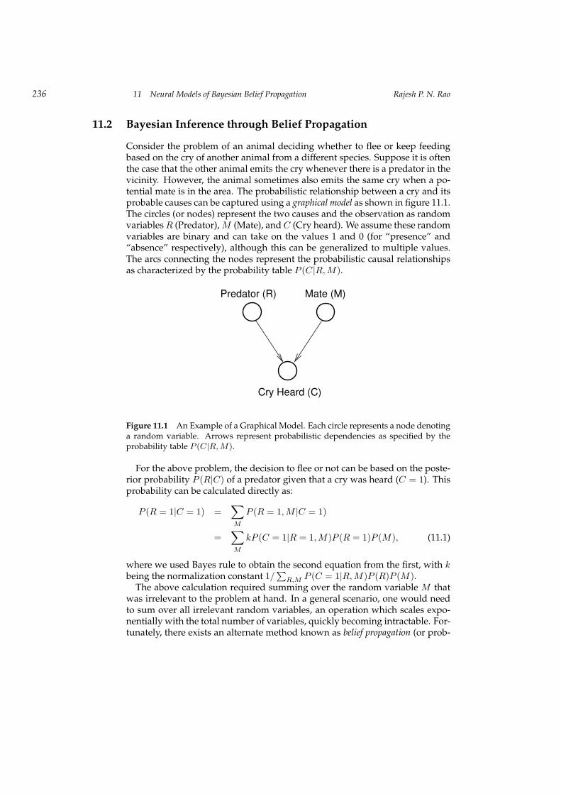
Consider the problem of an animal deciding whether to flee or keep feedingbased on the cry of another animal from a different species. Suppose it is oftenthe case that the other animal emits the cry whenever there is a predator in thevicinity. However, the animal sometimes also emits the same cry when a po-tential mate is in the area. The probabilistic relationship between a cry and itsprobable causes can be captured using a graphical model as shown in figure 11.1.The circles (or nodes) represent the two causes and the observation as randomvariablesR (Predator),M (Mate), andC (Cry heard). We assume these randomvariables are binary and can take on the values 1 and 0 (for “presence” and“absence” respectively), although this can be generalized to multiple values.The arcs connecting the nodes represent the probabilistic causal relationshipsas characterized by the probability table P (C|R,M).

Predator (R) Mate (M)

Cry Heard (C)

Figure 11.1 An Example of a Graphical Model. Each circle represents a node denotinga random variable. Arrows represent probabilistic dependencies as specified by theprobability table P (C|R, M).

For the above problem, the decision to flee or not can be based on the poste-rior probability P (R|C) of a predator given that a cry was heard (C = 1). Thisprobability can be calculated directly as:

P (R = 1|C = 1) =∑

M

P (R = 1,M |C = 1)

=∑

M

kP (C = 1|R = 1,M)P (R = 1)P (M), (11.1)

where we used Bayes rule to obtain the second equation from the first, with kbeing the normalization constant 1/

∑R,M P (C = 1|R,M)P (R)P (M).

The above calculation required summing over the random variable M thatwas irrelevant to the problem at hand. In a general scenario, one would needto sum over all irrelevant random variables, an operation which scales expo-nentially with the total number of variables, quickly becoming intractable. For-tunately, there exists an alternate method known as belief propagation (or prob-

11.2 Bayesian Inference through Belief Propagation 237

ability propagation) [26] that involves passing messages (probability vectors)between the nodes of the graphical model and summing over local productsof messages, an operation that can be tractable. The belief propagation algo-rithm involves two types of computation: marginalization (summation overlocal joint distributions) and multiplication of local marginal probabilities. Be-cause the operations are local, the algorithm is also well suited to neural im-plementation, as we shall discuss below. The algorithm is provably correct forsingly connected graphs (i.e., no undirected cycles) [26], although it has beenused with some success in some graphical models with cycles as well [25].

11.2.1 A Simple Example

We illustrate the belief propagation algorithm using the feed-or-flee problemabove. The nodes R and M first generate the messages P (R) and P (M) re-spectively, which are vectors of length two storing the prior probabilities forR = 0 and 1, and M = 0 and 1 respectively. These messages are sent to nodeC. Since a cry was heard, the value of C is known (C = 1) and therefore, themessages from R and M do not affect node C. We are interested in computingthe marginal probabilities for the two hidden nodes R and M . The node Cgenerates the message mC→R = mC→M = (0, 1), i.e., probability of absence ofa cry is 0 and probability of presence of a cry is 1 (since a cry was heard). Thismessage is passed on to the nodes R and M .

Each node performs a marginalization over variables other than itself usingthe local conditional probability table and the incoming messages. For exam-ple, in the case of node R, this is

∑M,C P (C|R,M)P (M)P (C) =

∑M P (C =

1|R,M)P (M) since C is known to be 1. Similarly, the node M performs themarginalization

∑R,C P (C|R,M)P (R)P (C) =

∑R P (C = 1|R,M)P (R). The

final step involves multiplying these marginalized probabilities with othermessages received, in this case, P (R) and P (M) respectively, to yield, after nor-malization, the posterior probability of R and M given the observation C = 1:

P (R|C = 1) = α(∑

M

P (C = 1|R,M)P (M))P (R) (11.2)

P (M |C = 1) = β(∑

R

P (C = 1|R,M)P (R))P (M), (11.3)

where α and β are normalization constants. Note that equation (11.2) aboveyields the same expression for P (R = 1|C = 1) as equation (11.1) that wasderived using Bayes rule. In general, belief propagation allows efficient com-putation of the posterior probabilities of unknown random variables in singlyconnected graphical models, given any available evidence in the form of ob-served values for any subset of the random variables.

11.2.2 Belief Propagation over Time

Belief propagation can also be applied to graphical models evolving over time.A simple but widely used model is the hidden Markov model (HMM) shown


in figure 11.2A. The input that is observed at time t (= 1, 2, . . .) is represented bythe random variable I(t), which can either be discrete-valued or a real-valuedvector such as an image or a speech signal. The input is assumed to be gen-erated by a hidden cause or “state” θ(t), which can assume one of N discretevalues 1, . . . , N . The state θ(t) evolves over time in a Markovian manner, de-pending only on the previous state according to the transition probabilitiesgiven by P (θ(t) = i|θ(t − 1) = j) = P (θti |θt−1

j ) for i, j = 1 . . . N . The observa-tion I(t) is generated according to the probability P (I(t)|θ(t)).

The belief propagation algorithm can be used to compute the posterior prob-ability of the state given current and past inputs (we consider here only the“forward” propagation case, corresponding to on-line state estimation). As inthe previous example, the node θt performs a marginalization over neighbor-ing variables, in this case θt−1 and I(t). The first marginalization results in aprobability vector whose ith component is

∑j P (θti |θt−1

j )mt−1,tj wheremt−1,t

j isthe jth component of the message from node θt−1 to θt. The second marginal-ization is from node I(t) and is given by

∑I(t) P (I(t)|θti)P (I(t)). If a particu-

lar input I′ is observed, this sum becomes∑

I(t) P (I(t)|θti)δ(I(t), I′) = P (I′|θti),where δ is the delta function which evaluates to 1 if its two arguments are equaland 0 otherwise. The two “messages” resulting from the marginalization alongthe arcs from θt−1 and I(t) can be multiplied at node θt to yield the followingmessage to θt+1:

mt,t+1i = P (I′|θti)

∑

j

P (θti |θt−1j )mt−1,t

j (11.4)

If m0,1i = P (θi) (the prior distribution over states), then it is easy to show using

Bayes rule that mt,t+1i = P (θti , I(t), . . . , I(1)).

Rather than computing the joint probability, one is typically interested incalculating the posterior probability of the state, given current and past inputs,i.e., P (θti |I(t), . . . , I(1)). This can be done by incorporating a normalization stepat each time step. Define (for t = 1, 2, . . .):

mti = P (I′|θti)

∑

j


j (11.5)

mt,t+1i = mt

i/nt, (11.6)

where nt =∑jm

tj . If m0,1

i = P (θi) (the prior distribution over states), then itis easy to see that:

mt,t+1i = P (θti |I(t), . . . , I(1)) (11.7)

This method has the additional advantage that the normalization at each timestep promotes stability, an important consideration for recurrent neuronal net-works, and allows the likelihood function P (I′|θti) to be defined in proportionalterms without the need for explicitly calculating its normalization factor (seesection 11.4 for an example).

11.2 Bayesian Inference through Belief Propagation 239

I(t+1)I(t)

A

t+1t

B

θt t+1θ

I(t)

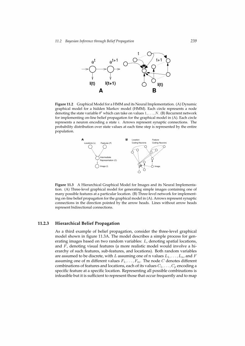
Figure 11.2 Graphical Model for a HMM and its Neural Implementation. (A) Dynamicgraphical model for a hidden Markov model (HMM). Each circle represents a nodedenoting the state variable θt which can take on values 1, . . . , N . (B) Recurrent networkfor implementing on-line belief propagation for the graphical model in (A). Each circlerepresents a neuron encoding a state i. Arrows represent synaptic connections. Theprobability distribution over state values at each time step is represented by the entirepopulation.

A LocationCoding Neurons Coding Neurons

Feature

Locations (L) Features (F)

IntermediateRepresentation (C)

Image

B

Image (I)

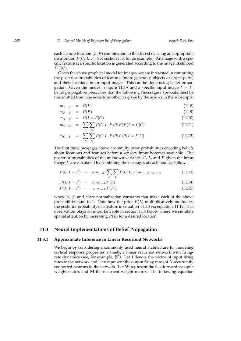
Figure 11.3 A Hierarchical Graphical Model for Images and its Neural Implementa-tion. (A) Three-level graphical model for generating simple images containing one ofmany possible features at a particular location. (B) Three-level network for implement-ing on-line belief propagation for the graphical model in (A). Arrows represent synapticconnections in the direction pointed by the arrow heads. Lines without arrow headsrepresent bidirectional connections.

11.2.3 Hierarchical Belief Propagation

As a third example of belief propagation, consider the three-level graphicalmodel shown in figure 11.3A. The model describes a simple process for gen-erating images based on two random variables: L, denoting spatial locations,and F , denoting visual features (a more realistic model would involve a hi-erarchy of such features, sub-features, and locations). Both random variablesare assumed to be discrete, with L assuming one of n values L1, . . . , Ln, and Fassuming one of m different values F1, . . . , Fm. The node C denotes differentcombinations of features and locations, each of its valuesC1, . . . , Cp encoding aspecific feature at a specific location. Representing all possible combinations isinfeasible but it is sufficient to represent those that occur frequently and to map


each feature-location (L,F ) combination to the closest Ci using an appropriatedistribution P (Ci|L,F ) (see section 11.4 for an example). An image with a spe-cific feature at a specific location is generated according to the image likelihoodP (I|C).

Given the above graphical model for images, we are interested in computingthe posterior probabilities of features (more generally, objects or object parts)and their locations in an input image. This can be done using belief propa-gation. Given the model in figure 11.3A and a specific input image I = I ′,belief propagation prescribes that the following ?messages? (probabilities) betransmitted from one node to another, as given by the arrows in the subscripts:

mL→C = P (L) (11.8)mF→C = P (F ) (11.9)mI→C = P (I = I ′|C) (11.10)

mC→L =∑

F

∑

C

P (C|L,F )P (F )P (I = I ′|C) (11.11)

mC→F =∑

L

∑

C

P (C|L,F )P (L)P (I = I ′|C) (11.12)

The first three messages above are simply prior probabilities encoding beliefsabout locations and features before a sensory input becomes available. Theposterior probabilities of the unknown variables C, L, and F given the inputimage I, are calculated by combining the messages at each node as follows:

P (C|I = I ′) = αmI→C∑

F

∑

L

P (C|L,F )mL→CmF→C (11.13)

P (L|I = I ′) = βmC→LP (L) (11.14)P (F |I = I ′) = γmC→FP (F ), (11.15)

where α, β, and γ are normalization constants that make each of the aboveprobabilities sum to 1. Note how the prior P (L) multiplicatively modulatesthe posterior probability of a feature in equation 11.15 via equation 11.12. Thisobservation plays an important role in section 11.4 below where we simulatespatial attention by increasing P (L) for a desired location.

11.3 Neural Implementations of Belief Propagation

11.3.1 Approximate Inference in Linear Recurrent Networks

We begin by considering a commonly used neural architecture for modelingcortical response properties, namely, a linear recurrent network with firing-rate dynamics (see, for example, [5]). Let I denote the vector of input firingrates to the network and let v represent the output firing rates of N recurrentlyconnected neurons in the network. Let W represent the feedforward synapticweight matrix and M the recurrent weight matrix. The following equation

11.3 Neural Implementations of Belief Propagation 241

describes the dynamics of the network:

τdvdt

= −v + WI + Uv, (11.16)

where τ is a time constant. The equation can be written in a discrete form asfollows:

vi(t+ 1) = vi(t) + ε(−vi(t) + wiI(t) +∑

j

uijvj(t)), (11.17)

where ε is the integration rate, vi is the ith component of the vector v, wi isthe ith row of the matrix W, and uij is the element of U in the ith row and jthcolumn. The above equation can be rewritten as:

vi(t+ 1) = εwiI(t) +∑

j

Uijvj(t), (11.18)

where Uij = εuij for i 6= j and Uii = 1 + ε(uii − 1). Comparing the beliefpropagation equation (11.5) for a HMM with equation (11.18) above, it can beseen that both involve propagation of quantities over time with contributionsfrom the input and activity from the previous time step. However, the beliefpropagation equation involves multiplication of these contributions while theleaky integrator equation above involves addition.

Now consider belief propagation in the log domain. Taking the logarithm ofboth sides of equation (11.5), we get:

logmti = logP (I′|θti) + log

∑

j


j (11.19)

This equation is much more conducive to neural implementation via equation(11.18). In particular, equation (11.18) can implement equation (11.19) if:

vi(t+ 1) = logmti (11.20)

εwiI(t) = logP (I′|θti) (11.21)∑

j

Uijvj(t) = log∑

j


j (11.22)

The normalization step (equation (11.6)) can be computed by a separate groupof neurons representing mt,t+1

i that receive as excitatory input logmti and in-

hibitory input log nt = log∑jm

tj :

logmt,t+1i = logmt

i − log nt (11.23)

These neurons convey the normalized posterior probabilities mt,t+1i back to

the neurons implementing equation (11.19) so that mt+1i may be computed at

the next time step. Note the the normalization step makes the overall networknonlinear.

In equation (11.21), the log-likelihood logP (I′|θti) is calculated using a lin-ear operation εwiI(t) (see also [45]). Since the messages are normalized at each


time step, one can relax the equality in equation (11.21) and make logP (I′|θti) ∝F(θi)I(t) for some linear filter F(θi) = εwi. This avoids the problem of calculat-ing the normalization factor for P (I′|θti), which can be especially hard when I′

takes on continuous values such as in an image. A more challenging problemis to pick recurrent weights Uij such that equation (11.22) holds true. For equa-tion (11.22) to hold true, we need to approximate a log-sum with a sum-of-logs.One approach is to generate a set of random probabilities xj(t) for t = 1, . . . , Tand find a set of weights Uij that satisfy:

∑

j

Uij log xj(t) ≈ log[∑

j

P (θti |θt−1j )xj(t)

](11.24)

for all i and t. This can be done by minimizing the squared error in equa-tion (11.24) with respect to the recurrent weights Uij . This empirical approach,followed in [30], is used in some of the experiments below. An alternative ap-proach is to exploit the nonlinear properties of dendrites as suggested in thefollowing section.

11.3.2 Exact Inference in Nonlinear Networks

A firing rate model that takes into account some of the effects of nonlinear fil-tering in dendrites can be obtained by generalizing equation (11.18) as follows:

vi(t+ 1) = f(wiI(t)

)+ g

(∑

j

Uijvj(t)), (11.25)

where f and g model nonlinear dendritic filtering functions for feedforwardand recurrent inputs. By comparing this equation with the belief propagationequation in the log domain (equation (11.19)), it can be seen that the first equa-tion can implement the second if:

vi(t+ 1) = logmti (11.26)

f(wiI(t)

)= logP (I′|θti) (11.27)

g(∑

j

Uijvj(t))

= log∑

j


j (11.28)

In this model (figure 11.2B), N neurons represent logmti (i = 1, . . . , N ) in their

firing rates. The dendritic filtering functions f and g approximate the loga-rithm function, the feedforward weights wi act as a linear filter on the inputto yield the likelihood P (I′|θti) and the recurrent synaptic weights Uij directlyencode the transition probabilities P (θti |θt−1

j ). The normalization step is com-puted as in equation (11.23) using a separate group of neurons that representlog posterior probabilities logmt,t+1

i and that convey these probabilities for usein equation (11.28) by the neurons computing logmt+1

i .

11.3 Neural Implementations of Belief Propagation 243

11.3.3 Inference Using Noisy Spiking Neurons

Spiking Neuron Model

The models above were based on firing rates of neurons, but a slight modifi-cation allows an interpretation in terms of noisy spiking neurons. Consider avariant of equation (11.16) where v represents the membrane potential valuesof neurons rather than their firing rates. We then obtain the classic equation de-scribing the dynamics of the membrane potential vi of neuron i in a recurrentnetwork of leaky integrate-and-fire neurons:

τdvidt

= −vi +∑

j

wijIj +∑

j

uijv′j , (11.29)

where τ is the membrane time constant, Ij denotes the synaptic current dueto input neuron j, wij represents the strength of the synapse from input j torecurrent neuron i, v′j denotes the synaptic current due to recurrent neuron j,and uij represents the corresponding synaptic strength. If vi crosses a thresholdT , the neuron fires a spike and vi is reset to the potential vreset. Equation (11.29)can be rewritten in discrete form as:

vi(t+ 1) = vi(t) + ε(−vi(t) +∑

j

wijIj(t)) +∑

j

uijv′j(t)) (11.30)

i.e. vi(t+ 1) = ε∑

j

wijIj(t) +∑

j

Uijv′j(t), (11.31)

where ε is the integration rate, Uii = 1 + ε(uii − 1) and for i 6= j, Uij = εuij .The nonlinear variant of the above equation that includes dendritic filtering ofinput currents in the dynamics of the membrane potential is given by:

vi(t+ 1) = f(∑

j

wijIj(t))

+ g(∑

j

Uijv′j(t)

), (11.32)

where f and g are nonlinear dendritic filtering functions for feedforward andrecurrent inputs.

We can model the effects of background inputs and the random openings ofmembrane channels by adding a Gaussian white noise term to the right-handside of equations (11.31) and (11.32). This makes the spiking of neurons inthe recurrent network stochastic. Plesser and Gerstner [27] and Gerstner [11]have shown that under reasonable assumptions, the probability of spiking insuch noisy neurons can be approximated by an “escape function” (or hazardfunction) that depends only on the distance between the (noise-free) membranepotential vi and the threshold T . Several different escape functions were foundto yield similar results. We use the following exponential function suggestedin [11] for noisy integrate-and-fire networks:

P (neuron i spikes at time t) = ke(vi(t)−T ), (11.33)

where k is an arbitrary constant. We use a model that combines equations(11.32) and (11.33) to generate spikes.


Inference in Spiking Networks

By comparing the membrane potential equation (11.32) with the belief prop-agation equation in the log domain (equation (11.19)), we can postulate thefollowing correspondences:

vi(t+ 1) = logmti (11.34)

f(∑

j

wijIj(t))

= logP (I′|θti) (11.35)

g(∑

j

Uijv′j(t)

)= log

∑

j


j (11.36)

The dendritic filtering functions f and g approximate the logarithm function,the synaptic currents Ij(t) and v′j(t) are approximated by the correspondinginstantaneous firing rates, and the recurrent synaptic weights Uij encode thetransition probabilities P (θti |θt−1

j ).Since the membrane potential vi(t+1) is assumed to be equal to logmt

i (equa-tion (11.34)), we can use equation (11.33) to calculate the probability of spikingfor each neuron i as:

P (neuron i spikes at time t+ 1) ∝ e(vi(t+1)−T ) (11.37)

∝ e(logmti−T ) (11.38)

∝ mti (11.39)

Thus, the probability of spiking (or, equivalently, the instantaneous firing rate)for neuron i in the recurrent network is directly proportional to the messagemt

i,which is the posterior probability of the neuron’s preferred state and currentinput given past inputs. Similarly, the instantaneous firing rates of the group ofneurons representing logmt,t+1

i is proportional tomt,t+1i , which is the precisely

the input required by equation (11.36).

11.4 Results

11.4.1 Example 1: Detecting Visual MotionWe first illustrate the application of the linear firing rate-based model (sec-tion 11.3.1) to the problem of detecting visual motion. A prominent propertyof visual cortical cells in areas such as V1 and MT is selectivity to the directionof visual motion. We show how the activity of such cells can be interpreted asrepresenting the posterior probability of stimulus motion in a particular direc-tion, given a series of input images. For simplicity, we focus on the case of 1Dmotion in an image consisting ofX pixels with two possible motion directions:leftward (L) or rightward (R).

Let the state θij represent a motion direction j ∈ {L,R} at spatial loca-tion i. Consider a network of N neurons, each representing a particular stateθij (figure 11.4A). The feedforward weights are assumed to be Gaussians, i.e.F(θiR) = F(θiL) = F(θi) = Gaussian centered at location i with a standard

11.4 Results 245

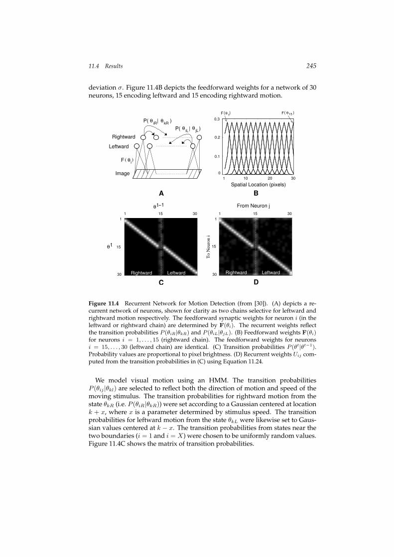
deviation σ. Figure 11.4B depicts the feedforward weights for a network of 30neurons, 15 encoding leftward and 15 encoding rightward motion.

5 10 15 20 25 30

5

10

15

20

25

305 10 15 20 25 30

5

10

15

20

25

30

0 5 10 15 20 25 300

0.1

0.2

0.3θkRθ iR

θ

iLθ θ jLP( | )

( )F θ1

BA

θ

θ

P( | )

( )F

Leftward

Rightward

Image

i

F( )θ15

Rightward LeftwardLeftward

From Neuron jT

o N

euro

n i

t−1

t

Rightward

Spatial Location (pixels)

151 30 151 30

0

0.1

0.2

0.3

1

15

30

15

1

30

20 30101

C D

Figure 11.4 Recurrent Network for Motion Detection (from [30]). (A) depicts a re-current network of neurons, shown for clarity as two chains selective for leftward andrightward motion respectively. The feedforward synaptic weights for neuron i (in theleftward or rightward chain) are determined by F(θi). The recurrent weights reflectthe transition probabilities P (θiR|θkR) and P (θiL|θjL). (B) Feedforward weights F(θi)for neurons i = 1, . . . , 15 (rightward chain). The feedforward weights for neuronsi = 15, . . . , 30 (leftward chain) are identical. (C) Transition probabilities P (θt|θt−1).Probability values are proportional to pixel brightness. (D) Recurrent weights Uij com-puted from the transition probabilities in (C) using Equation 11.24.

We model visual motion using an HMM. The transition probabilitiesP (θij |θkl) are selected to reflect both the direction of motion and speed of themoving stimulus. The transition probabilities for rightward motion from thestate θkR (i.e. P (θiR|θkR)) were set according to a Gaussian centered at locationk + x, where x is a parameter determined by stimulus speed. The transitionprobabilities for leftward motion from the state θkL were likewise set to Gaus-sian values centered at k − x. The transition probabilities from states near thetwo boundaries (i = 1 and i = X) were chosen to be uniformly random values.Figure 11.4C shows the matrix of transition probabilities.


Recurrent Network Model

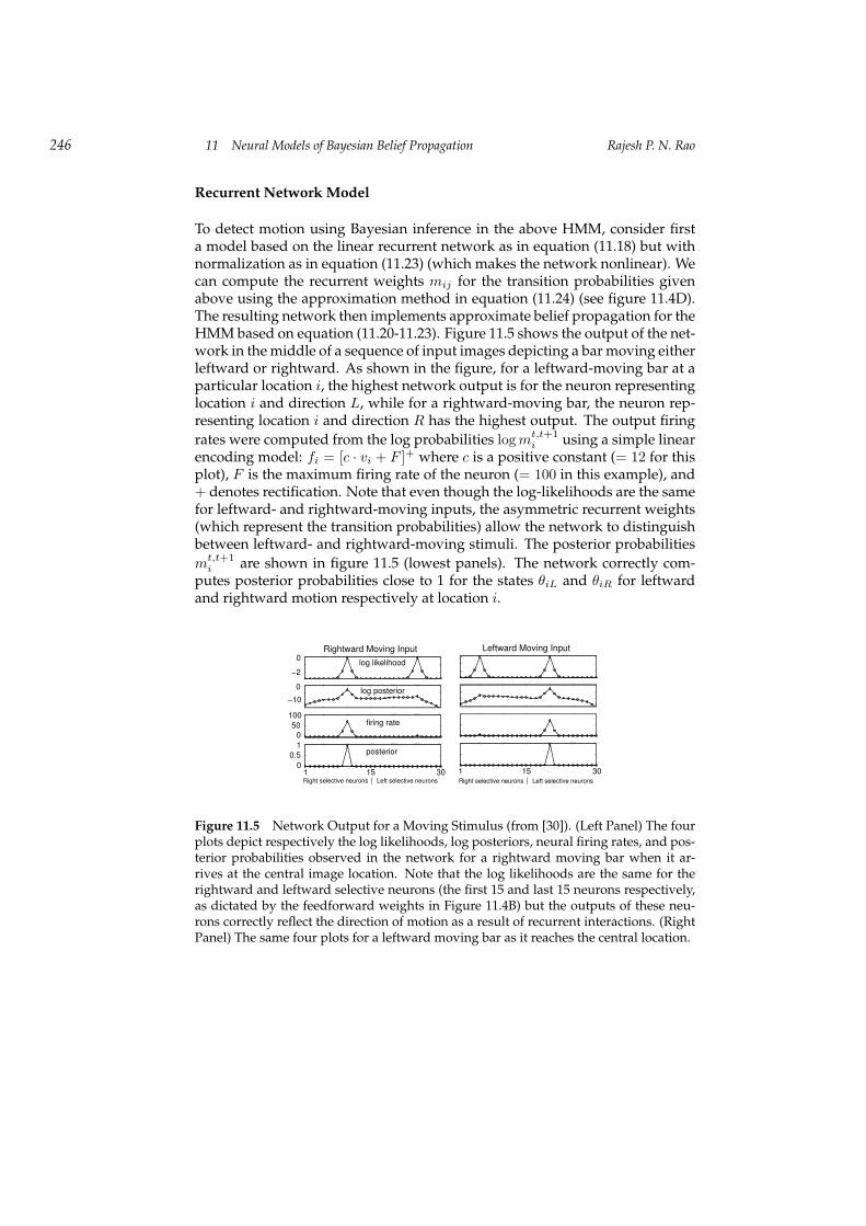
To detect motion using Bayesian inference in the above HMM, consider firsta model based on the linear recurrent network as in equation (11.18) but withnormalization as in equation (11.23) (which makes the network nonlinear). Wecan compute the recurrent weights mij for the transition probabilities givenabove using the approximation method in equation (11.24) (see figure 11.4D).The resulting network then implements approximate belief propagation for theHMM based on equation (11.20-11.23). Figure 11.5 shows the output of the net-work in the middle of a sequence of input images depicting a bar moving eitherleftward or rightward. As shown in the figure, for a leftward-moving bar at aparticular location i, the highest network output is for the neuron representinglocation i and direction L, while for a rightward-moving bar, the neuron rep-resenting location i and direction R has the highest output. The output firingrates were computed from the log probabilities logmt,t+1

i using a simple linearencoding model: fi = [c · vi + F ]+ where c is a positive constant (= 12 for thisplot), F is the maximum firing rate of the neuron (= 100 in this example), and+ denotes rectification. Note that even though the log-likelihoods are the samefor leftward- and rightward-moving inputs, the asymmetric recurrent weights(which represent the transition probabilities) allow the network to distinguishbetween leftward- and rightward-moving stimuli. The posterior probabilitiesmt,t+1i are shown in figure 11.5 (lowest panels). The network correctly com-

putes posterior probabilities close to 1 for the states θiL and θiR for leftwardand rightward motion respectively at location i.

5 10 15 20 25 30−15−10−5

0

5 10 15 20 25 300

50

100

5 10 15 20 25 300

0.5

1

5 10 15 20 25 30

−2−1

0

5 10 15 20 25 30−15−10−5

0

5 10 15 20 25 300

50

100

5 10 15 20 25 300

0.5

1

5 10 15 20 25 30

−2−1

0

Right selective neurons Left selective neurons

log likelihood

log posterior

firing rate

posterior

Leftward Moving InputRightward Moving Input

Right selective neurons Left selective neurons

1

0

0

−2

0.5

0

0

−10

100

1 15 130 3015

50

Figure 11.5 Network Output for a Moving Stimulus (from [30]). (Left Panel) The fourplots depict respectively the log likelihoods, log posteriors, neural firing rates, and pos-terior probabilities observed in the network for a rightward moving bar when it ar-rives at the central image location. Note that the log likelihoods are the same for therightward and leftward selective neurons (the first 15 and last 15 neurons respectively,as dictated by the feedforward weights in Figure 11.4B) but the outputs of these neu-rons correctly reflect the direction of motion as a result of recurrent interactions. (RightPanel) The same four plots for a leftward moving bar as it reaches the central location.

11.4 Results 247

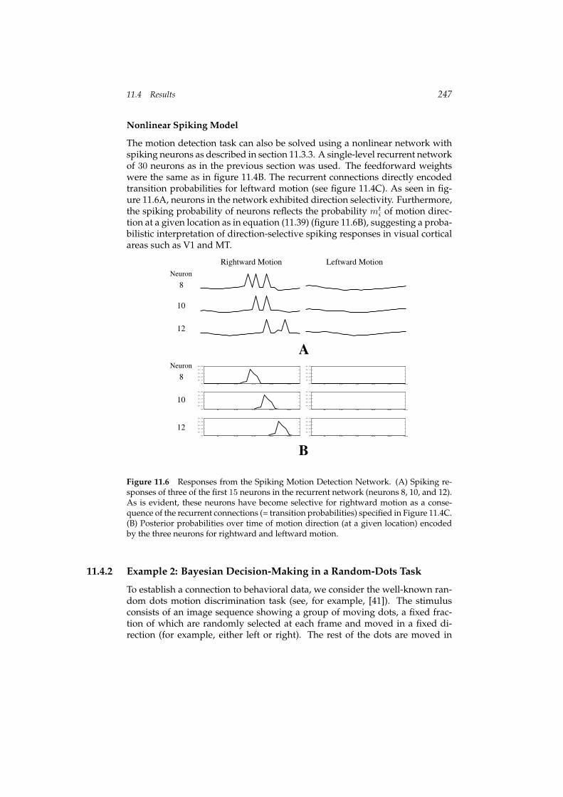
Nonlinear Spiking Model

The motion detection task can also be solved using a nonlinear network withspiking neurons as described in section 11.3.3. A single-level recurrent networkof 30 neurons as in the previous section was used. The feedforward weightswere the same as in figure 11.4B. The recurrent connections directly encodedtransition probabilities for leftward motion (see figure 11.4C). As seen in fig-ure 11.6A, neurons in the network exhibited direction selectivity. Furthermore,the spiking probability of neurons reflects the probability mt

i of motion direc-tion at a given location as in equation (11.39) (figure 11.6B), suggesting a proba-bilistic interpretation of direction-selective spiking responses in visual corticalareas such as V1 and MT.

5 10 15 20 250

0.1

0.2

0.3

0.4

0.5

5 10 15 20 250

0.1

0.2

0.3

0.4

0.5

5 10 15 20 250

0.1

0.2

0.3

0.4

0.5

5 10 15 20 25 300

0.1

0.2

0.3

0.4

0.5

5 10 15 20 25 300

0.1

0.2

0.3

0.4

0.5

5 10 15 20 25 300

0.1

0.2

0.3

0.4

0.5

8Neuron

10

12

8Neuron

12

10

Rightward Motion Leftward Motion

B

A

Figure 11.6 Responses from the Spiking Motion Detection Network. (A) Spiking re-sponses of three of the first 15 neurons in the recurrent network (neurons 8, 10, and 12).As is evident, these neurons have become selective for rightward motion as a conse-quence of the recurrent connections (= transition probabilities) specified in Figure 11.4C.(B) Posterior probabilities over time of motion direction (at a given location) encodedby the three neurons for rightward and leftward motion.

11.4.2 Example 2: Bayesian Decision-Making in a Random-Dots Task

To establish a connection to behavioral data, we consider the well-known ran-dom dots motion discrimination task (see, for example, [41]). The stimulusconsists of an image sequence showing a group of moving dots, a fixed frac-tion of which are randomly selected at each frame and moved in a fixed di-rection (for example, either left or right). The rest of the dots are moved in


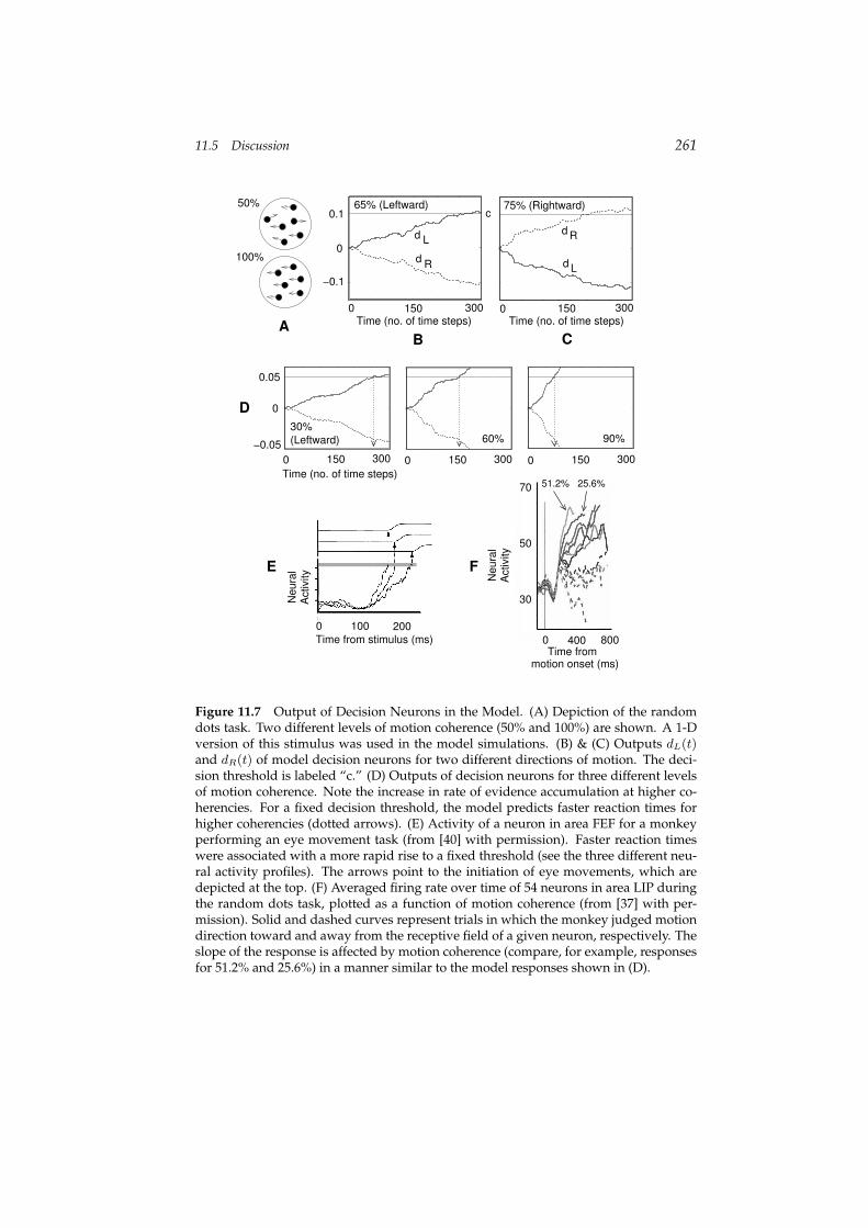
random directions. The fraction of dots moving in the same direction is calledthe coherence of the stimulus. Figure 11.7A depicts the stimulus for two dif-ferent levels of coherence. The task is to decide the direction of motion of thecoherently moving dots for a given input sequence. A wealth of data exists onthe psychophysical performance of humans and monkeys as well as the neuralresponses in brain areas such as the middle temporal (MT) and lateral intra-parietal areas (LIP) in monkeys performing the task (see [41] and referencestherein). Our goal is to explore the extent to which the proposed models forneural belief propagation can explain the existing data for this task.

The nonlinear motion detection network in the previous section computesthe posterior probabilities P (θiL|I(t), . . . , I(1)) and P (θiR|I(t), . . . , I(1)) of left-ward and rightward motion at different locations i. These outputs can be usedto decide the direction of coherent motion by computing the posterior prob-abilities for leftward and rightward motion irrespective of location, given theinput images. These probabilities can be computed by marginalizing the pos-terior distribution computed by the neurons for leftward (L) and rightward (R)motion over all spatial positions i:

P (L|I(t), . . . , I(1)) =∑

i

P (θiL|I(t), . . . , I(1)) (11.40)

P (R|I(t), . . . , I(1)) =∑

i

P (θiR|I(t), . . . , I(1)) (11.41)

To decide the overall direction of motion in a random-dots stimulus, thereexist two options: (1) view the decision process as a “race” between the twoprobabilities above to a prechosen threshold (this also generalizes to more thantwo choices); or (2) compute the log of the ratio between the two probabilitiesabove and compare this log-posterior ratio to a prechosen threshold. We usethe latter method to allow comparison to the results of Shadlen and colleagues,who postulate a ratio-based model in area LIP in primate parietal cortex [12].The log-posterior ratio r(t) of leftward over rightward motion can be definedas:

r(t) = logP (L|I(t), . . . , I(1))− logP (R|I(t), . . . , I(1)) (11.42)

= logP (L|I(t), . . . , I(1))P (R|I(t), . . . , I(1))

(11.43)

If r(t) > 0, the evidence seen so far favors leftward motion and vice versa forr(t) < 0. The instantaneous ratio r(t) is susceptible to rapid fluctuations dueto the noisy stimulus. We therefore use the following decision variable dL(t) totrack the running average of the log posterior ratio of L over R:

dL(t+ 1) = dL(t) + α(r(t)− dL(t)) (11.44)

and likewise for dR(t) (the parameter α is between 0 and 1). We assume thatthe decision variables are computed by a separate set of “decision neurons”that receive inputs from the motion detection network. These neurons are once

11.4 Results 249

again leaky-integrator neurons as described by Equation 11.44, with the driv-ing inputs r(t) being determined by inhibition between the summed inputsfrom the two chains in the motion detection network (as in equation (11.42)).The output of the model is “L” if dL(t) > c and “R” if dR(t) > c, where c isa “confidence threshold” that depends on task constraints (for example, accu-racy vs. speed requirements) [35].

Figure 11.7B and C shows the responses of the two decision neurons overtime for two different directions of motion and two levels of coherence. Be-sides correctly computing the direction of coherent motion in each case, themodel also responds faster when the stimulus has higher coherence. This phe-nomenon can be appreciated more clearly in figure 11.7D, which predicts pro-gressively shorter reaction times for increasingly coherent stimuli (dotted ar-rows).

Comparison to Neurophysiological Data

The relationship between faster rates of evidence accumulation and shorter re-action times has received experimental support from a number of studies. Fig-ure 11.7E shows the activity of a neuron in the frontal eye fields (FEF) for fast,medium, and slow responses to a visual target [39, 40]. Schall and collabora-tors have shown that the distribution of monkey response times can be repro-duced using the time taken by neural activity in FEF to reach a fixed threshold[15]. A similar rise-to-threshold model by Carpenter and colleagues has re-ceived strong support in human psychophysical experiments that manipulatethe prior probabilities of targets [3] and the urgency of the task [35].

In the case of the random-dots task, Shadlen and collaborators have shownthat in primates, one of the cortical areas involved in making the decision re-garding coherent motion direction is area LIP. The activities of many neurons inthis area progressively increase during the motion-viewing period, with fasterrates of rise for more coherent stimuli (see figure 11.7F) [37]. This behavior issimilar to the responses of “decision neurons” in the model (figure 11.7B–D),suggesting that the outputs of the recorded LIP neurons could be interpretedas representing the log-posterior ratio of one task alternative over another (see[3, 12] for related suggestions).

11.4.3 Example 3: Attention in the Visual Cortex

The responses of neurons in cortical areas V2 and V4 can be significantly mod-ulated by attention to particular locations within an input image. McAdamsand Maunsell [23] showed that the tuning curve of a neuron in cortical area V4is multiplied by an approximately constant factor when the monkey focusesattention on a stimulus within the neuron’s receptive field. Reynolds et al. [36]have shown that focusing attention on a target in the presence of distractorscauses the response of a V2 or V4 neuron to closely approximate the responseelicited when the target appears alone. Finally, a study by Connor et al. [4]demonstrated that responses to unattended stimuli can be affected by spatial


attention to nearby locations.All three types of response modulation described above can be explained in

terms of Bayesian inference using the hierarchical graphical model for imagesgiven in section 11.2.3 (figure 11.3). Each V4 neuron is assumed to encode afeature Fi as its preferred stimulus. A separate group of neurons (e.g., in theparietal cortex) is assumed to encode spatial locations (and potentially otherspatiotemporal transformations) irrespective of feature values. Lower-levelneurons (for example, in V2 and V1) are assumed to represent the interme-diate representations Ci. Figure 11.3B depicts the corresponding network forneural belief propagation. Note that this network architecture mimics the di-vision of labor between the ventral object processing ("what") stream and thedorsal spatial processing ("where") stream in the visual cortex [24].

The initial firing rates of location- and feature-coding neurons representprior probabilities P (L) and P (F ) respectively, assumed to be set by task-dependent feedback from higher areas such as those in prefrontal cortex. Theinput likelihood P (I = I ′|C) is set to

∑j wijIj , where the weights wij repre-

sent the attributes of Ci (specific feature at a specific location). Here, we setthese weights to spatially localized oriented Gabor filters. equation (11.11) and(11.12) are assumed to be computed by feedforward neurons in the location-coding and feature-coding parts of the network, with their synapses encod-ing P (C|L,F ). Taking the logarithm of both sides of equations (11.13-11.15),we obtain equations that can be computed using leaky integrator neurons asin equation (11.32) (f and g are assumed to approximate a logarithmic trans-formation). Recurrent connections in equation (11.32) are used to implementthe inhibitory component corresponding to the negative logarithm of the nor-malization constants. Furthermore, since the membrane potential vi(t) is nowequal to the log of the posterior probability, i.e., vi(t) = logP (F |I = I ′) (andsimilarly for L and C), we obtain, using equation (11.33):

P (feature coding neuron i spikes at time t) ∝ P (F |I = I ′) (11.45)

This provides a new interpretation of the spiking probability (or instantaneousfiring rate) of a V4 neuron as representing the posterior probability of a pre-ferred feature in an image (irrespective of spatial location).

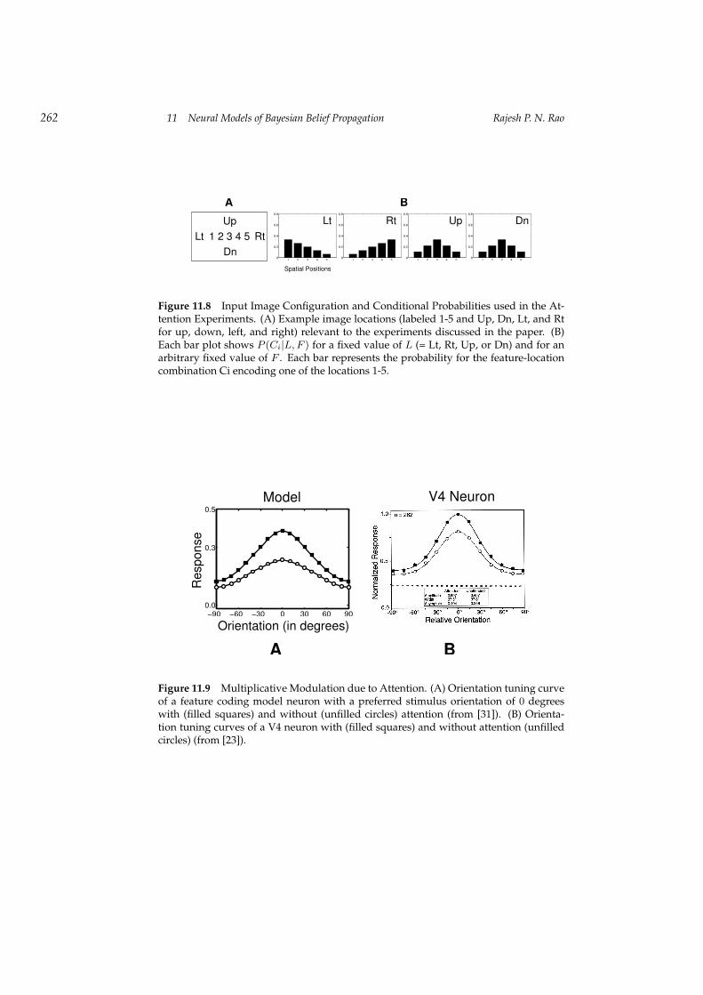
To model the three primate experiments discussed above [4, 23, 36], we usedhorizontal and vertical bars that could appear at nine different locations in theinput image (figure 11.8A). All results were obtained using a network with asingle set of parameters. P (C|L,F ) was chosen such that for any given valueof L and F , say location Lj and feature Fk, the value of C closest to the combi-nation (Lj , Fk) received the highest probability, with decreasing probabilitiesfor neighboring locations (see figure 11.8B).

Multiplicative Modulation of Responses

We simulated the attentional task of McAdams and Maunsell [23] by present-ing a vertical bar and a horizontal bar simultaneously in an input image. “At-tention” to a location Li containing one of the bars was simulated by setting

11.4 Results 251

a high value for P (Li), corresponding to a higher firing rate for the neuroncoding for that location.

Figure 11.9A depicts the orientation tuning curves of the vertical feature cod-ing model V4 neuron in the presence and absence of attention (squares andcircles respectively). The plotted points represent the neuron’s firing rate, en-coding the posterior probability P (F |I = I ′), F being the vertical feature. At-tention in the model approximately multiplies the “unattended” responses bya constant factor, similar to V4 neurons (figure 11.9B). This is due to the changein the prior P (L) between the two modes, which affects equation (11.12) and(11.15) multiplicatively.

Effects of Attention on Responses in the Presence of Distractors

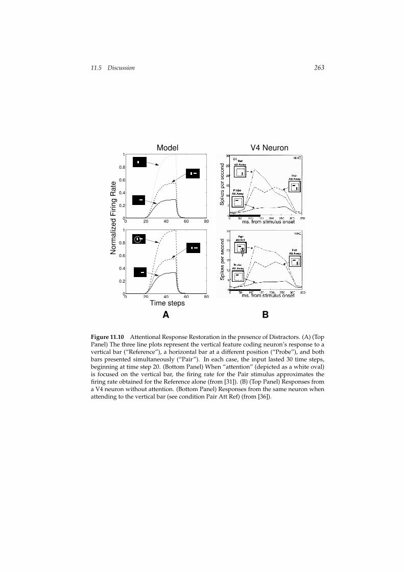
To simulate the experiments of Reynolds et al. [36], a single vertical bar (“Refer-ence”) were presented in the input image and the responses of the vertical fea-ture coding model neuron were recorded over time. As seen in figure 11.10A(top panel, dotted line), the neuron’s firing rate reflects a posterior probabil-ity close to 1 for the vertical stimulus. When a horizontal bar (“Probe”) aloneis presented at a different location, the neuron’s response drops dramatically(solid line) since its preferred stimulus is a vertical bar, not a horizontal bar.When the horizontal and vertical bars are simultaneously presented (“Pair”),the firing rate drops to almost half the value elicited for the vertical bar alone(dashed line), signaling increased uncertainty about the stimulus compared tothe Reference-only case. However, when “attention” is turned on by increas-ing P (L) for the vertical bar location (figure 11.10A, bottom panel), the firingrate is restored back to its original value and a posterior probability close to 1is signaled (topmost plot, dot-dashed line). Thus, attention acts to reduce un-certainty about the stimulus given a location of interest. Such behavior closelymimics the effect of spatial attention in areas V2 and V4 [36] (figure 11.10B).

Effects of Attention on Neighboring Spatial Locations

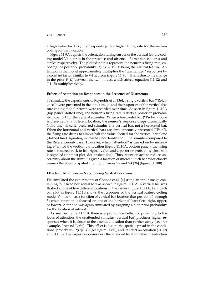
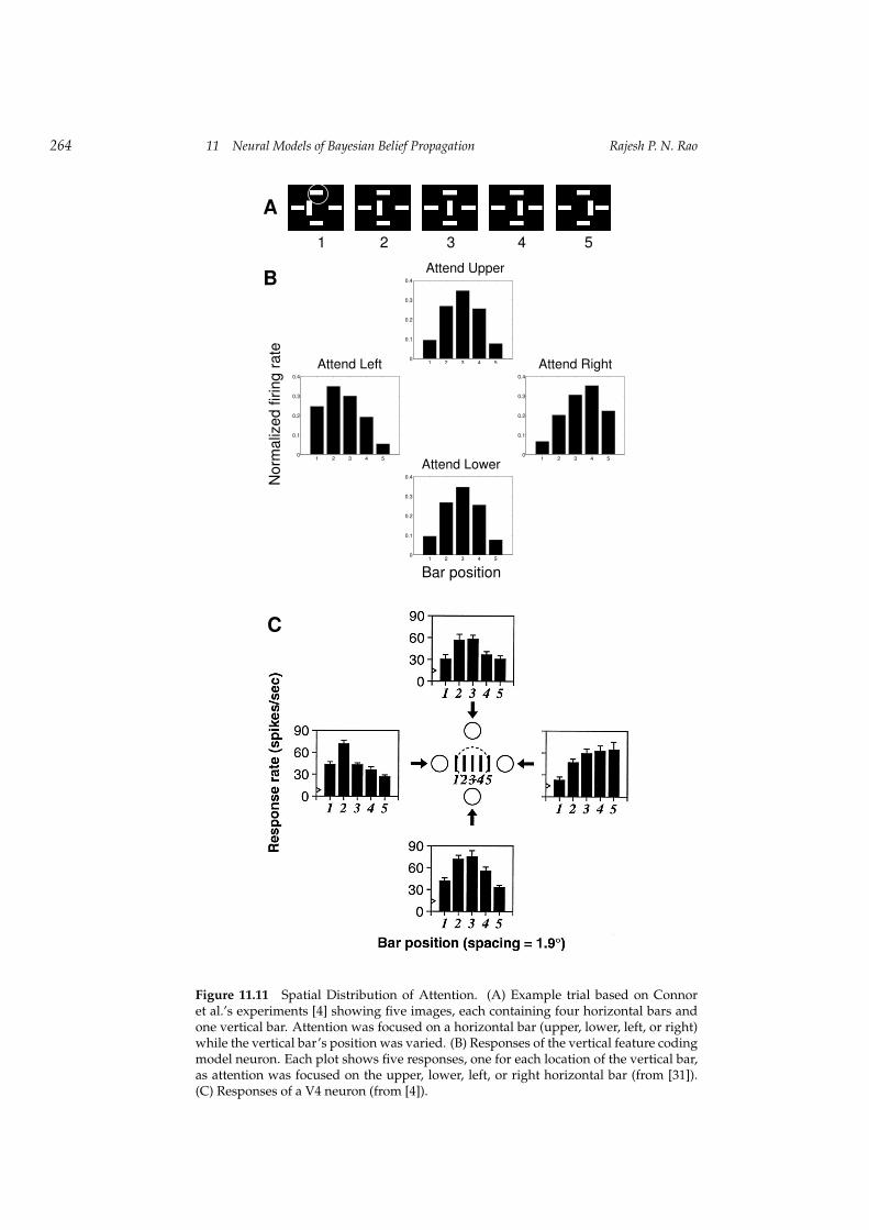
We simulated the experiments of Connor et al. [4] using an input image con-taining four fixed horizontal bars as shown in figure 11.11A. A vertical bar wasflashed at one of five different locations in the center (figure 11.11A, 1-5). Eachbar plot in figure 11.11B shows the responses of the vertical feature codingmodel V4 neuron as a function of vertical bar location (bar positions 1 through5) when attention is focused on one of the horizontal bars (left, right, upper,or lower). Attention was again simulated by assigning a high prior probabilityfor the location of interest.

As seen in figure 11.11B, there is a pronounced effect of proximity to thelocus of attention: the unattended stimulus (vertical bar) produces higher re-sponses when it is closer to the attended location than further away (see, forexample, “Attend Left”). This effect is due to the spatial spread in the condi-tional probability P (C|L,F ) (see figure 11.8B), and its effect on equation (11.12)and (11.15). The larger responses near the attended location reflect a reduction


in uncertainty at locations closer to the focus of attention compared to locationsfarther away. For comparison, the responses from a V4 neuron are shown infigure 11.11C (from [4]).

11.5 Discussion

This chapter described models for neurally implementing the belief propaga-tion algorithm for Bayesian inference in arbitrary graphical models. Linear andnonlinear models based on firing rate dynamics, as well as a model based onnoisy spiking neurons, were presented. We illustrated the suggested approachin two domains: (1) inference over time using an HMM and its application tovisual motion detection and decision-making, and (2) inference in a hierarchi-cal graphical model and its application to understanding attentional effects inthe primate visual cortex.

The approach suggests an interpretation of cortical neurons as computingthe posterior probability of their preferred state, given current and past in-puts. In particular, the spiking probability (or instantaneous firing rate) of aneuron can be shown to be directly proportional to the posterior probabilityof the preferred state. The model also ascribes a functional role to local re-current connections (lateral/horizontal connections) in the neocortex: connec-tions from excitatory neurons are assumed to encode transition probabilitiesbetween states from one time step to the next, while inhibitory connections areused for probability normalization (see equation (11.23)). Similarly, feedbackconnections from higher to lower areas are assumed to convey prior proba-bilities reflecting prior knowledge or task constraints, as used in the attentionmodel in section 11.4.3.

11.5.1 Related Models

A number of models have been proposed for probabilistic computation innetworks of neuron-like elements. These range from early models based onstatistical mechanics (such as the Boltzmann machine [19, 20]) to more re-cent models that explicitly rely on probabilistic generative or causal models[6, 10, 29, 33, 43, 44, 45]. We review in more detail some of the models that areclosely related to the approach presented in this chapter.

Models based on Log-Likelihood Ratios

Gold and Shadlen [12] have proposed a model for neurons in area LIP thatinterprets their responses as representing the log-likelihood ratio betweentwo alternatives. Their model is inspired by neurophysiological results fromShadlen’s group and others showing that the responses of neurons in area LIPexhibit a behavior similar to a random walk to a fixed threshold. The neuron’sresponse increases given evidence in favor of the neuron’s preferred hypoth-esis and decreases when given evidence against that hypothesis, resulting in

11.5 Discussion 253

an evidence accumulation process similar to computing a log-likelihood ratioover time (see section 11.4.2). Gold and Shadlen develop a mathematical model[12] to formalize this intuition. They show how the log-likelihood ratio can bepropagated over time as evidence trickles in at each time instant. This model issimilar to the one proposed above involving log-posterior ratios for decision-making. The main difference is in the representation of probabilities. Whilewe explicitly maintain a representation of probability distributions of relevantstates using populations of neurons, the model of Gold and Shadlen relies onthe argument that input firing rates can be directly interpreted as log-likelihoodratios without the need for explicit representation of probabilities.

An extension of the Gold and Shadlen model to the case of spiking neuronswas recently proposed by Deneve [8]. In this model, each neuron is assumedto represent the log-“odds” ratio for a preferred binary-valued state, i.e., thelogarithm of the probability that the preferred state is 1 over the probabilitythat the preferred state is 0, given all inputs seen thus far. To promote efficiency,each neuron fires only when the difference between its log-odds ratio and aprediction of the log-odds ratio (based on the output spikes emitted thus far)reaches a certain threshold.

Models based on log-probability ratios such as the ones described abovehave several favorable properties. First, since only ratios are represented, onemay not need to normalize responses at each step to ensure probabilities sumto 1 as in an explicit probability code. Second, the ratio representation lends it-self naturally to some decision-making procedures such as the one postulatedby Gold and Shadlen. However, the log-probability ratio representation alsosuffers from some potential shortcomings. Because it is a ratio, it is susceptibleto instability when the probability in the denominator approaches zero (a logprobability code also suffers from a similar problem), although this can be han-dled using bounds on what can be represented by the neural code. Also, theapproach becomes inefficient when the number of hypotheses being consid-ered is large, given the large number of ratios that may need to be representedcorresponding to different combinations of hypotheses. Finally, the lack of anexplicit probability representation means that many useful operations in prob-ability calculus, such as marginalization or uncertainty estimation in specificdimensions, could become complicated to implement.

Inference Using Distributional Codes

There has been considerable research on methods for encoding and decodinginformation from populations of neurons. One class of methods uses basisfunctions (or “kernels”) to represent probability distributions within neuronalensembles [1, 2, 9]. In this approach, a distribution P (x) over stimulus x isrepresented using a linear combination of basis functions:

P (x) =∑

i

ribi(x), (11.46)


where ri is the normalized response (firing rate) and bi the implicit basis func-tion associated with neuron i in the population. The basis function of eachneuron is assumed to be linearly related to the tuning function of the neuron asmeasured in physiological experiments. The basis function approach is similarto the approach described in this chapter in that the stimulus space is spannedby a limited number of neurons with preferred stimuli or state vectors. Thetwo approaches differ in how probability distributions are represented by neu-ral responses, one using an additive method and the other using a logarith-mic transformation either in the firing rate representation (sections 11.3.1 and11.3.2) or in the membrane potential representation (section 11.3.3).

A limitation of the basis function approach is that due to its additive na-ture, it cannot represent distributions that are sharper than the component dis-tributions. A second class of models addresses this problem using a genera-tive approach, where an encoding model (e.g., Poisson) is first assumed anda Bayesian decoding model is used to estimate the stimulus x (or its distribu-tion), given a set of responses ri [28, 46, 48, 49, 51]. For example, in the distribu-tional population coding (DPC) method [48, 49], the responses are assumed todepend on general distributions P (x) and a maximimum a posteriori (MAP)probability distribution over possible distributions over x is computed. Thebest estimate in this method is not a single value of x but an entire distribu-tion over x, which is assumed to be represented by the neural population. Theunderlying goal of representing entire distributions within neural populationsis common to both the DPC approach and the models presented in this chap-ter. However, the approaches differ in how they achieve this goal: the DPCmethod assumes prespecified tuning functions for the neurons and a sophisti-cated, non-neural decoding operation, whereas the method introduced in thischapter directly instantiates a probabilistic generative model with an exponen-tial or linear decoding operation. Sahani and Dayan have recently extendedthe DPC method to the case where there is uncertainty as well as simultane-ous multiple stimuli present in the input [38]. Their approach, known as dou-bly distributional population coding (DDPC), is based on encoding probabilitydistributions over a function m(x) of the input x rather than distributions overx itself. Needless to say, the greater representational capacity of this methodcomes at the expense of more complex encoding and decoding schemes.

The distributional coding models discussed above were geared primarily to-ward representing probability distributions. More recent work by Zemel andcolleagues [50] has explored how distributional codes could be used for infer-ence as well. In their approach, a recurrent network of leaky integrate-and-fire neurons is trained to capture the probabilistic dynamics of a hidden vari-able X(t) by minimizing the Kullback-Leibler (KL) divergence between an in-put encoding distribution P (X(t)|R(t)) and an output decoding distributionQ(X(t)|S(t)), where R(t) and S(t) are the input and output spike trains re-spectively. The advantage of this approach over the models presented in thischapter is that the decoding process may allow a higher-fidelity representationof the output distribution than the direct representational scheme used in thischapter. On the other hand, since the probability representation is implicit in

11.5 Discussion 255

the neural population, it becomes harder to map inference algorithms such asbelief propagation to neural circuitry.

Hierarchical Inference

There has been considerable interest in neural implementation of hierarchicalmodels for inference. Part of this interest stems from the fact that hierarchicalmodels often capture the multiscale structure of input signals such as images ina very natural way (e.g., objects are composed of parts, which are composed ofsubparts,..., which are composed of edges). A hierarchical decomposition oftenresults in greater efficiency, both in terms of representation (e.g., a large num-ber of objects can be represented by combining the same set of parts in manydifferent ways) and in terms of learning. A second motivation for hierarchicalmodels has been the evidence from anatomical and physiological studies thatmany regions of the primate cortex are hierarchically organized (e.g., the visualcortex, motor cortex, etc.).

Hinton and colleagues investigated a hierarchical network called theHelmholtz machine [16] that uses feedback connections from higher to lowerlevels to instantiate a probabilistic generative model of its inputs (see also [18]).An interesting learning algorithm termed the “wake-sleep” algorithm was pro-posed that involved learning the feedback weights during a “wake” phasebased on inputs and the feedforward weights in the “sleep” phase based on“fantasy” data produced by the feedback model. Although the model employsfeedback connections, these are used only for bootstrapping the learning of thefeedforward weights (via fantasy data). Perception involves a single feedfor-ward pass through the network and the feedback connections are not used forinference or top-down modulation of lower-level activities.

A hierarchical network that does employ feedback for inference was ex-plored by Lewicki and Sejnowski [22] (see also [17] for a related model). TheLewicki-Sejnowski model is a Bayesian belief network where each unit encodesa binary state and the probability that a unit’s state Si is equal to 1 depends onthe states of its parents pa[Si] via:

P (Si = 1|pa[Si],W ) = h(∑

j

wjiSj), (11.47)

where W is the matrix of weights, wji is the weight from Sj to Si (wji = 0 forj < i), and h is the noisy OR function h(x) = 1 − e−x (x ≥ 0). Rather thaninferring a posterior distribution over states as in the models presented in thischapter, Gibbs sampling is used to obtain samples of states from the posterior;the sampled states are then used to learn the weights wji.

Rao and Ballard proposed a hierarchical generative model for images andexplored an implementation of inference in this model based on predictivecoding [34]. Unlike the models presented in this chapter, the predictive cod-ing model focuses on estimating the MAP value of states rather than an en-tire distribution. More recently, Lee and Mumford sketched an abstract hier-archical model [21] for probabilistic inference in the visual cortex based on an


inference method known as particle filtering. The model is similar to our ap-proach in that inference involves message passing between different levels, butwhereas the particle-filtering method assumes continuous random variables,our approach uses discrete random variables. The latter choice allows a con-crete model for neural representation and processing of probabilities, while itis unclear how a biologically plausible network of neurons can implement thedifferent components of the particle filtering algorithm.

The hierarchical model for attention described in section 11.4.3 bears somesimilarities to a recent Bayesian model proposed by Yu and Dayan [47] (seealso [7, 32]). Yu and Dayan use a five-layer neural architecture and a log proba-bility encoding scheme as in [30] to model reaction time effects and multiplica-tive response modulation. Their model, however, does not use an interme-diate representation to factor input images into separate feature and locationattributes. It therefore cannot explain effects such as the influence of attentionon neighboring unattended locations [4]. A number of other neural modelsexist for attention, e.g., models by Grossberg and colleagues [13, 14], that aremuch more detailed in specifying how various components of the model fitwith cortical architecture and circuitry. The approach presented in this chaptermay be viewed as a first step toward bridging the gap between detailed neuralmodels and more abstract Bayesian theories of perception.

11.5.2 Open Problems and Future Challenges

An important open problem not addressed in this chapter is learning and adap-tation. How are the various conditional probability distributions in a graphicalmodel learned by a network implementing Bayesian inference? For instance,in the case of the HMM model used in section 11.4.1, how can the transitionprobabilities between states from one time step to the next be learned? Canwell-known biologically plausible learning rules such as Hebbian learning orthe Bienenstock-Cooper-Munro (BCM) rule (e.g., see [5]) be used to learn con-ditional probabilities? What are the implications of spike-timing dependentplasticity (STDP) and short-term plasticity on probabilistic representations inneural populations?

A second open question is the use of spikes in probabilistic representations.The models described above were based directly or indirectly on instantaneousfiring rates. Even the noisy spiking model proposed in section 11.3.3 can beregarded as encoding posterior probabilities in terms of instantaneous firingrates. Spikes in this model are used only as a mechanism for communicat-ing information about firing rate over long distances. An intriguing alternatepossibility that is worth exploring is whether probability distributions can beencoded using spike timing-based codes. Such codes may be intimately linkedto timing-based learning mechanisms such as STDP.

Another interesting issue is how the dendritic nonlinearities known to existin cortical neurons could be exploited to implement belief propagation as inequation (11.19). This could be studied systematically with a biophysical com-partmental model of a cortical neuron by varying the distribution and densities

11.5 Discussion 257

of various ionic channels along the dendrites.Finally, this chapter explored neural implementations of Bayesian inference

in only two simple graphical models (HMMs and a three-level hierarchicalmodel). Neuroanatomical data gathered over the past several decades pro-vide a rich set of clues regarding the types of graphical models implicit inbrain structure. For instance, the fact that visual processing in the primatebrain involves two hierarchical but interconnected pathways devoted to spa-tial and object vision (the “what” and “where” streams) [24] suggests a mul-tilevel graphical model wherein the input image is factored into progressivelycomplex sets of object features and their transformations. Similarly, the ex-istence of multimodal areas in the inferotemporal cortex suggests graphicalmodels that incorporate a common modality-independent representation atthe highest level that is causally related to modality-dependent representa-tions at lower levels. Exploring such graphical models that are inspired byneurobiology could not only shed new light on brain function but also furnishnovel architectures for solving fundamental problems in machine vision androbotics.

Acknowledgments This work was supported by grants from the ONR Adap-tive Neural Systems program, NSF, NGA, the Sloan Foundation, and thePackard Foundation.

References

[1] Anderson CH (1995) Unifying perspectives on neuronal codes and processing. In 19thInternational Workshop on Condensed Matter Theories. Caracas, Venezuela.

[2] Anderson CH, Van Essen DC (1994) Neurobiological computational systems. In Zu-rada JM, Marks II RJ, Robinson CJ, eds., Computational Intelligence: Imitating Life,pages 213–222, New York: IEEE Press.

[3] Carpenter RHS, Williams MLL (1995) Neural computation of log likelihood in controlof saccadic eye movements. Nature, 377:59–62.

[4] Connor CE, Preddie DC, Gallant JL, Van Essen DC (1997) Spatial attention effects inmacaque area V4. Journal of Neuroscience, 17:3201–3214.

[5] Dayan P, Abbott LF (2001) Theoretical Neuroscience: Computational and Mathematical Mod-eling of Neural Systems. Cambridge, MA: MIT Press.

[6] Dayan P, Hinton G, Neal R, Zemel R (1995) The Helmholtz machine. Neural Computa-tion, 7:889–904.

[7] Dayan P, Zemel R (1999) Statistical models and sensory attention. In Willshaw D,Murray A, eds., Proceedings of the International Conference on Artificial Neural Networks(ICANN), pages 1017–1022, London: IEEE Press.

[8] Deneve S (2005) Bayesian inference in spiking neurons. In Saul LK, Weiss Y, Bottou L,eds., Advances in Neural Information Processing Systems 17, pages 353–360, Cambridge,MA: MIT Press.

[9] Eliasmith C, Anderson CH (2003) Neural Engineering: Computation, Representation, andDynamics in Neurobiological Systems. Cambridge, MA: MIT Press.


[10] Freeman WT, Haddon J, Pasztor EC (2002) Learning motion analysis. In ProbabilisticModels of the Brain: Perception and Neural Function, pages 97–115, Cambridge, MA:MIT Press.

[11] Gerstner W (2000) Population dynamics of spiking neurons: Fast transients, asyn-chronous states, and locking. Neural Computation, 12(1):43–89.

[12] Gold JI, Shadlen MN (2001) Neural computations that underlie decisions about sen-sory stimuli. Trends in Cognitive Sciences, 5(1):10–16.

[13] Grossberg S (2005) Linking attention to learning, expectation, competition, and con-sciousness. In Neurobiology of Attention, pages 652–662. San Diego: Elsevier.

[14] Grossberg S, Raizada R (2000) Contrast-sensitive perceptual grouping and object-based attention in the laminar circuits of primary visual cortex. Vision Research,40:1413–1432.

[15] Hanes DP, Schall JD (1996) Neural control of voluntary movement initiation. Science,274:427–430.

[16] Hinton G, Dayan P, Frey B, Neal R (1995) The wake-sleep algorithm for unsupervisedneural networks. Science, 268:1158–1161.

[17] Hinton G, Ghahramani Z (1997) Generative models for discovering sparse distributedrepresentations. Philosophical Transactions of the Royal Society of London, Series B.,352:1177–1190.

[18] Hinton G, Osindero S, Teh Y (2006) A fast learning algorithm for deep belief nets.Neural Computation, 18:1527–1554.

[19] Hinton G, Sejnowski T (1983) Optimal perceptual inference. In Proceedings of the IEEEConference on Computer Vision and Pattern Recognition, pages 448–453, Washington DC1983, New York: IEEE Press.

[20] Hinton G, Sejnowski T (1986) Learning and relearning in Boltzmann machines. InRumelhart D, McClelland J, eds., Parallel Distributed Processing, volume 1, chapter 7,pages 282–317, Cambridge, MA: MIT Press.

[21] Lee TS, Mumford D (2003) Hierarchical Bayesian inference in the visual cortex. Journalof the Optical Society of America A, 20(7):1434–1448.

[22] Lewicki MS, Sejnowski TJ (1997) Bayesian unsupervised learning of higher orderstructure. In Mozer M, Jordan M, Petsche T, eds., Advances in Neural Information Pro-cessing Systems 9, Cambridge, MA: MIT Press.

[23] McAdams CJ, Maunsell JHR (1999) Effects of attention on orientation-tuning func-tions of single neurons in macaque cortical area V4. Journal of Neuroscience, 19:431–441.

[24] Mishkin M, Ungerleider LG, Macko KA (1983) Object vision and spatial vision: twocortical pathways. Trends in Neuroscience, 6:414–417.

[25] Murphy K, Weiss Y, Jordan M (1999) Loopy belief propagation for approximate infer-ence: an empirical study. In Laskey K, Prade H eds., Proceedings of UAI (Uncertaintyin AI), pages 467–475, San Francisco: Morgan Kaufmann.

[26] Pearl J (1988) Probabilistic Reasoning in Intelligent Systems: Networks of Plausible Infer-ence. San Mateo: CA,Morgan Kaufmann.

[27] Plesser HE, Gerstner W (2000) Noise in integrate-and-fire neurons: from stochasticinput to escape rates. Neural Computation, 12(2):367–384, .

11.5 Discussion 259

[28] Pouget A, Zhang K, Deneve S, Latham PE (1998) Statistically efficient estimation usingpopulation coding. Neural Computation, 10(2):373–401.

[29] Rao RPN (1999) An optimal estimation approach to visual perception and learning.Vision Research, 39(11):1963–1989.

[30] Rao RPN (2004) Bayesian computation in recurrent neural circuits. Neural Computa-tion, 16(1):1–38.

[31] Rao RPN (2005) Bayesian inference and attentional modulation in the visual cortex.Neuroreport, 16(16):1843–1848.

[32] Rao RPN (2005) Hierarchical Bayesian inference in networks of spiking neurons. InSaul LK, Weiss Y, Bottou L, eds., Advances in Neural Information Processing Systems 17,pages 1113–1120, Cambridge, MA: MIT Press.

[33] Rao RPN, Ballard DH (1997) Dynamic model of visual recognition predicts neuralresponse properties in the visual cortex. Neural Computation, 9(4):721–763.

[34] Rao RPN, Ballard DH (1999) Predictive coding in the visual cortex: a functional inter-pretation of some extra-classical receptive field effects. Nature Neuroscience, 2(1):79–87.

[35] Reddi BA, Carpenter RH (2000) The influence of urgency on decision time. NatureNeuroscience, 3(8):827–830.

[36] Reynolds JH, Chelazzi L, Desimone R (1999) Competitive mechanisms subserve at-tention in macaque areas V2 and V4. Journal of Neuroscience, 19:1736–1753.

[37] Roitman JD, Shadlen MN (2002) Response of neurons in the lateral intraparietal areaduring a combined visual discrimination reaction time task. Journal of Neuroscience,22:9475–9489.

[38] Sahani M, Dayan P (2003) Doubly distributional population codes: simultaneousrepresentation of uncertainty and multiplicity. Neural Computation, 15:2255–2279.

[39] Schall JD, Hanes DP (1998) Neural mechanisms of selection and control of visuallyguided eye movements. Neural Networks, 11:1241–1251.

[40] Schall JD, Thompson KG (1999) Neural selection and control of visually guided eyemovements. Annual Review of Neuroscience, 22:241–259.

[41] Shadlen MN, Newsome WT (2001) Neural basis of a perceptual decision in the parietalcortex (area LIP) of the rhesus monkey. Journal of Neurophysiology, 86(4):1916–1936.

[42] Shon AP, Rao RPN (2005) Implementing belief propagation in neural circuits. Neuro-computing, 65-66:393–399.

[43] Simoncelli EP (1993) Distributed Representation and Analysis of Visual Motion. PhD the-sis, Department of Electrical Engineering and Computer Science, MIT, Cambridge,MA.

[44] Weiss Y, Fleet DJ (2002) Velocity likelihoods in biological and machine vision. In RaoRPN, Olshausen BA, Lewicki MS, eds., Probabilistic Models of the Brain: Perception andNeural Function, pages 77–96, Cambridge, MA: MIT Press.

[45] Weiss Y, Simoncelli EP, Adelson EH (2002) Motion illusions as optimal percepts. Na-ture Neuroscience, 5(6):598–604.

[46] Wu S, Chen D, Niranjan M, Amari SI (2003) Sequential Bayesian decoding with apopulation of neurons. Neural Computation, 15.


[47] Yu A, Dayan P (2005) Inference, attention, and decision in a Bayesian neural archi-tecture. In Saul LK, Weiss Y, Bottou L, eds., Advances in Neural Information ProcessingSystems 17, pages 1577–1584. Cambridge, MA: MIT Press, 2005.

[48] Zemel RS, Dayan P (1999) Distributional population codes and multiple motion mod-els. In Kearns MS, Solla SA, Cohn DA, eds., Advances in Neural Information ProcessingSystems 11, pages 174–180, Cambridge, MA: MIT Press.

[49] Zemel RS, Dayan P, Pouget A (1998) Probabilistic interpretation of population codes.Neural Computation, 10(2):403–430.

[50] Zemel RS, Huys QJM, Natarajan R, Dayan P (2005) Probabilistic computation in spik-ing populations. In Saul LK, Weiss Y, Bottou L, eds., Advances in Neural InformationProcessing Systems 17, pages 1609–1616. Cambridge, MA: MIT Press.

[51] Zhang K, Ginzburg I, McNaughton BL, Sejnowski TJ (1998) Interpreting neuronalpopulation activity by reconstruction: A unified framework with application to hip-pocampal place cells. Journal of Neurophysiology, 79(2):1017–1044.

11.5 Discussion 261

50 100 150 200 250 300−0.05

0

0.05

50 100 150 200 250 300−0.05

0

0.05

50 100 150 200 250 300

−0.1

0

0.1

50 100 150 200 250 300−0.05

0

0.05

50 100 150 200 250 300

−0.1

0

0.1

Time (no. of time steps) Time (no. of time steps)

25.6%51.2%

Neu

ral

Act

ivity N

eura

lA

ctiv

ity

d

d

d LR

R

75% (Rightward)65% (Leftward)

d L

A

100%

50%

60% 90%30%

CB

(Leftward)

E

Time from stimulus (ms)Time from

motion onset (ms)

F

D

Time (no. of time steps)

30

50

70

0

0

−0.05

0.05

0.1

−0.1

300150 300150 3001500 0 0

c

300 150 3001500 0

0 100 2004000 800

Figure 11.7 Output of Decision Neurons in the Model. (A) Depiction of the randomdots task. Two different levels of motion coherence (50% and 100%) are shown. A 1-Dversion of this stimulus was used in the model simulations. (B) & (C) Outputs dL(t)and dR(t) of model decision neurons for two different directions of motion. The deci-sion threshold is labeled “c.” (D) Outputs of decision neurons for three different levelsof motion coherence. Note the increase in rate of evidence accumulation at higher co-herencies. For a fixed decision threshold, the model predicts faster reaction times forhigher coherencies (dotted arrows). (E) Activity of a neuron in area FEF for a monkeyperforming an eye movement task (from [40] with permission). Faster reaction timeswere associated with a more rapid rise to a fixed threshold (see the three different neu-ral activity profiles). The arrows point to the initiation of eye movements, which aredepicted at the top. (F) Averaged firing rate over time of 54 neurons in area LIP duringthe random dots task, plotted as a function of motion coherence (from [37] with per-mission). Solid and dashed curves represent trials in which the monkey judged motiondirection toward and away from the receptive field of a given neuron, respectively. Theslope of the response is affected by motion coherence (compare, for example, responsesfor 51.2% and 25.6%) in a manner similar to the model responses shown in (D).


1 2 3 4 50

0.2

0.4

0.6

0.8

1 2 3 4 50

0.2

0.4

0.6

0.8

1 2 3 4 50

0.2

0.4

0.6

0.8

1 2 3 4 50

0.2

0.4

0.6

0.8

21 3 4 5 RtLtUp DnRtLtUp

Dn

BA

Spatial Positions

Figure 11.8 Input Image Configuration and Conditional Probabilities used in the At-tention Experiments. (A) Example image locations (labeled 1-5 and Up, Dn, Lt, and Rtfor up, down, left, and right) relevant to the experiments discussed in the paper. (B)Each bar plot shows P (Ci|L, F ) for a fixed value of L (= Lt, Rt, Up, or Dn) and for anarbitrary fixed value of F . Each bar represents the probability for the feature-locationcombination Ci encoding one of the locations 1-5.

−90 −60 −30 0 30 60 900.0

0.3

0.5

Res

pons

e

Model V4 Neuron

Orientation (in degrees)

A B

Figure 11.9 Multiplicative Modulation due to Attention. (A) Orientation tuning curveof a feature coding model neuron with a preferred stimulus orientation of 0 degreeswith (filled squares) and without (unfilled circles) attention (from [31]). (B) Orienta-tion tuning curves of a V4 neuron with (filled squares) and without attention (unfilledcircles) (from [23]).

11.5 Discussion 263

0 20 40 60 800

0.2

0.4

0.6

0.8

1

0 20 40 60 800

0.2

0.4

0.6

0.8

1Model V4 Neuron

Nor

mal

ized

Firi

ng R

ate

Time steps

A B

Figure 11.10 Attentional Response Restoration in the presence of Distractors. (A) (TopPanel) The three line plots represent the vertical feature coding neuron’s response to avertical bar (“Reference”), a horizontal bar at a different position (“Probe”), and bothbars presented simultaneously (“Pair”). In each case, the input lasted 30 time steps,beginning at time step 20. (Bottom Panel) When “attention” (depicted as a white oval)is focused on the vertical bar, the firing rate for the Pair stimulus approximates thefiring rate obtained for the Reference alone (from [31]). (B) (Top Panel) Responses froma V4 neuron without attention. (Bottom Panel) Responses from the same neuron whenattending to the vertical bar (see condition Pair Att Ref) (from [36]).


1 2 3 4 5

1 2 3 4 50

0.1

0.2

0.3

0.4

1 2 3 4 50

0.1

0.2

0.3

0.4

1 2 3 4 50

0.1

0.2

0.3

0.4

1 2 3 4 50

0.1

0.2

0.3

0.4Nor

mal

ized

firin

g ra

teAttend Upper

Attend Right

Attend Lower

Bar position

Attend Left

C

A

B

Figure 11.11 Spatial Distribution of Attention. (A) Example trial based on Connoret al.’s experiments [4] showing five images, each containing four horizontal bars andone vertical bar. Attention was focused on a horizontal bar (upper, lower, left, or right)while the vertical bar’s position was varied. (B) Responses of the vertical feature codingmodel neuron. Each plot shows five responses, one for each location of the vertical bar,as attention was focused on the upper, lower, left, or right horizontal bar (from [31]).(C) Responses of a V4 neuron (from [4]).

Index

acausal, 122attention, 101attention, Bayesian model of, 249average cost per stage, 273

Bayes filter, 9Bayes rule, 298Bayes theorem, 6Bayesian decision making, 247Bayesian estimate, 8, 9Bayesian estimator, 114Bayesian inference, 235Bayesian network, 12belief propagation, 12, 235belief state, 285bell-shape, 111Bellman equation, 267Bellman error, 272bias, 113bit, 6

causal, 122coding, 112conditional probability, 4continuous-time Riccati equation, 281contraction mapping, 268contrasts, 94control gain, 282convolution code, 119convolution decoding, 121convolution encoding, 119correlation, 5costate, 274covariance, 4Cramér-Rao bound, 113, 115Cramér-Rao inequality, 11cross-validation, 65curse of dimensionality, 272

decision theory, 295decoding, 53, 112decoding basis function, 121deconvolution, 120differential dynamic programming,

282direct encoding, 117discounted cost, 273discrete-time Riccati equation, 282discrimination threshold, 116distributional codes, 253distributional population code, 117doubly distributional population code,

121Dynamic Causal Modeling (DCM), 103dynamic programming, 266

economics, 295EEG, 91encoding, 112entropy, 7estimation-control duality, 287Euler-Lagrange equation, 278evidence, 12expectation, 4expectation-maximization, 121extended Kalman filter, 285extremal trajectory, 275

filter gain, 284firing rate, 112Fisher Information, 11Fisher information, 115fMRI, 91Fokker-Planck equation, 286

gain of population activity, 118general linear model, 91

318 Index

generalized linear model (GLM), 60graphical model, 12

Hamilton equation, 278Hamilton-Jacobi-Bellman equation,

271Hamiltonian, 275hemodynamic response function, 92hidden Markov model, 238, 285hierarchical inference, 255hyperparameter, 12hypothesis, 6

importance sampling, 285independence, 5influence function, 277information, 6information filter, 284information state, 285integrate-and-fire model, generalized,

62iterative LQG, 282Ito diffusion, 269Ito lemma, 271

joint probability, 4

Kalman filter, 9, 283Kalman smoother, 285Kalman-Bucy filter, 284kernel function, 119KL divergence, 8Kolmogorov equation, 286Kullback-Leiber divergence, 8

Lagrange multiplier, 276law of large numbers, 118Legendre transformation, 278likelihood, 6linear-quadratic regulator, 281log posterior ratio, 248loss function, 114

MAP, 8marginal likelihood, 12marginalization, 12Markov decision process, 269mass-univariate, 91maximum a posterior estimate, 8maximum a posteriori estimator, 67

maximum aposterior estimator, 287maximum entropy, 122maximum likelihood, 55, 114maximum likelihood estimate, 8maximum likelihood Estimator, 114maximum principle, 273mean, 4MEG, 91Mexican hat kernel, 120minimal variance, 114minimum-energy estimator, 287MLE, 8model selection, 12model-predictive control, 276motion energy, 118multiplicity, 121mutual information, 7

neural coding problem, 53

optimality principle, 266optimality value function, 266

particle filter, 9, 285Poisson distribution, 112Poisson noise, 115Poisson process, 56policy iteration, 267population code, 111population codes, 111population vector, 113posterior distribution, 114posterior probability, 6posterior probability mapping(PPM),

99preferred orientation, 111PrimerMarginal, 12prior distribution, 114prior probability, 6probabilistic population code, 118probability, 3probability density, 3probability distribution, 3product of expert, 122

random field, 122random field theory (RFT), 99Rauch recursion, 285recurrent network, linear, 240recurrent network, nonlinear, 242

Index 319

regularization, 11reverse correlation, 56rollout policy, 276

spike count, 112spike-triggered average (STA), 56spike-triggered covariance (STC), 58spiking neuron model, 243square-root filter, 284statistical parametric mapping (SPM),

99stimulus decoding, 113stimulus encoding, 112sufficient statistics, 285

temporally changing probability, 122time-rescaling, 53tuning curve, 111, 114

unbiased, 114unbiased estimate, 115uncertainty, 7, 116, 118, 120, 296unscented filter, 285utility, 296

value iteration, 267variance, 4, 113variance components , 97visual attention, 249visual motion detection, 244Viterbi algorithm, 287

Zakai’s equation, 286

neural models of bayesian belief propagation rajesh - washington

Documents