Staged Financing with a Variable Return

By Vladimir Smirnov and Andrew Wait∗

January 2006

Abstract

This paper explores the hold-up problem between two parties (an entrepreneurand an investor) when one of the parties (the entrepreneur) is unable to commitnot to repudiate the initial contract. To mitigate hold-up we allow the parties tostage investments over time and derive the optimal investment path in a modelthat places no restrictions on the growth of collateral. Our model predicts thatneither positive wealth of the entrepreneur nor the lack of discounting ensuresthat all profitable projects proceed. We also derive necessary and sufficientconditions for the project to be financeable when there are no costs of delay.Key words: hold-up, staged financing, investment policy. JEL classifications:G31, M13.

1 Introduction

An entrepreneur might have a great idea but not have the money to execute it.Consider, for instance, a cash-constrained entrepreneur who has access to a profitableinvestment project that can produce a certain return R = sK in one period, wheres is a constant rate of return greater than one and K is the cost of physical capitalrequired to complete the project. With no wealth the entrepreneur has no choice butto find an outside investor to finance the project, who must receive a large enoughpart of the return so as to at least cover her costs. A problem can arise, however, ifthe initial agreement between the entrepreneur and the investor is not enforceable.In this case the entrepreneur may repudiate the initial contract by threatening towithdraw his human capital from the project. Anticipating this renegotiation (orhold-up problem), the investor will not finance some profitable projects (see Hart andMoore 1994).

∗Discipline of Economics, University of Sydney NSW 2006 AUSTRALIA. Email:v.smirnov@econ.usyd.edu.au and a.wait@econ.usyd.edu.au. We would like to thank Murali Agastya,Matt Benge, Steve Dowrick, Kris Funston, Simon Grant, Flavio Menezes, Rohan Pitchford, MatthewRyan and Kunal Sengupta for their very useful comments.

1

To illustrate this point, consider the following example. The rate of return s isequal to 1.8 and total cost of capital investment K is equal to $1. The entrepreneurborrows $1 from the investor and promises to return $1 to her in one period. After theinvestor lends the money the entrepreneur repudiates the initial agreement, causingthe parties to renegotiate. Renegotiation occurs after the up-front investment (of$1) is sunk but prior to the realization of the return of the project. For simplicity,assume that both agents have equal bargaining powers. As the investment is sunkthe investor will receive half of the final return, that is sK/2 = $0.9, which is lessthan the total capital invested. Consequently, the investor will not provide up-frontfinance for an otherwise profitable project.

In an important contribution Neher (1999) showed that financing a project instages can help mitigate this commitment problem by allowing the accumulationof alienable physical assets to be used as collateral by the investor in the event ofrenegotiation. To illustrate this point, assume the entrepreneur stages the capitalinvestment such that γK dollars, where γ ∈ (0, 1), are invested immediately and theremaining (1− γ)K dollars are invested in one period’s time. Such a project returnsR = sK dollars in two periods. The output produced in the first period can beused as collateral in the second period. This collateral reassures the investor thatthe entrepreneur will not repudiate the initial agreement in the second period. First-period repudiation will also not occur because the entrepreneur’s net return withrepudiation is smaller than his net return specified in the initial contract. Hence, theinvestor may be able to finance the project with the investment staged in two rounds,which is something she would not be willing to do if all the investment had to beprovided up-front.

Let us go back to our example and show that it is possible to finance the project in2 stages. Let the up-front investment be I1 = $0.6 and the investment in one periodtime be I2 = $0.4. The entrepreneur receives R = $1.8 over the two periods andpromises to pay back the investor $1; the entrepreneur’s net return is $0.8. What ifthe entrepreneur repudiates the initial contract straight after I1 has been invested? I1

is sunk and the net return of the project is R− I2 = $1.4. As both parties have equalbargaining powers the entrepreneur receives 1

2(R−I2) = $0.7 and the investor receives

the remainder, that is I2 + 12(R − I2) = $1.1. The entrepreneur’s return in the case

of repudiation is smaller than his return specified in the initial contract. Therefore,he has no incentive to repudiate the initial contract in the first period. What if theentrepreneur repudiates the initial contract after I2 has been invested? In this casethe investor has an option to liquidate the project and receive the output from thefirst period. The return of the investor is sI1 = $1.08, which is greater than her costs.Again, the entrepreneur has no incentive to repudiate the initial contract. In thismanner the investor can finance the project in two stages, which was not possibleusing a single investment period.

In essence, staged investment allows the entrepreneur’s inalienable human capitalto be converted into tangible physical assets, increasing the investor’s collateral inevent of repudiation. Furthermore, the entrepreneur does not want to trigger rene-gotiation because his return is greater if the project continues. Neher (1999)assumed

2

that the rate of return for the project and the accumulated assets to be used as collat-eral alike is constant. More realistically, returns may differ significantly over differentstages of the project. A non-constant rate of return allows for an examination of awider scope of projects including, for example, projects with fixed costs or increasingand decreasing rates of return.1 As shown below, relaxing the assumption of constantreturns significantly alters the predictions concerning the optimal investment path -this is the main contribution of this paper. For instance, Neher (1999) predicts thatpositive wealth of the entrepreneur and a lack of discounting (very short time durationof one period) ensures that all profitable projects go forward. On the contrary, themodel presented here shows that this is not the case. Unlike in Neher, if the projectdoes not produce enough collateral in the early investment periods the project willnot be financed, even if it is profitable. This arises because the conversion of the en-trepreneur’s human capital in early periods is relatively low, the investor will not beafforded sufficient collateral protection, and the entrepreneur will have an incentiveto repudiate the original contract.

Another difference arises with respect to the optimal investment path itself whenwe allow for a more general relationship between investment and collateral. Ne-her (1999) finds that, starting from the second investment, the optimal investmentpath is always monotonically increasing. The result presented here is that the optimalinvestment path in general is not monotonically increasing with respect to the size ofthe investment. In both models the values of investments are determined by the waycollateral accumulates. However, if collateral accumulates in at a decreasing rate, thesequence of investments will be decreasing as well.

We derive necessary and sufficient conditions for the project to be financed whenthere are no costs of delay. We also identify the different roles of the final return ofthe project and collateral that accrues to the investor. The investment in the firstperiod is supported by the final return. Once the project has commenced, however,further investments are supported by the collateral.

The issue of commitment has been examined in a number of other papers. Hartand Moore (1994) constructed a model in which the capital borrowed from the investorplus entrepreneur’s wealth are invested by the entrepreneur at the beginning of thefirst period. This investment generates a stream of nonnegative returns and a streamof nonnegative liquidation values. The returns promised to the investor may not becredible as the entrepreneur cannot commit not to remove his valuable human capitalfrom the project and renegotiate the investor’s return. If in some period the outcomeof renegotiation leaves the investor with a combined return less than his investmentminus returns he has already received, he would not be willing to finance the projectex ante. Solving for all possible repayment paths such that the entrepreneur hasno incentive to repudiate, the authors show how repayment paths change with thematurity structure of the project return stream, and with durability and specificity

1For example, the human capital of a researcher working on a new innovation may only becometangible when it can be converted into an alienable asset, like a patent. Research will not necessarilybe converted into patents at a constant rate - it may be that only after certain stages of the projectthe researcher’s (or entrepreneur’s) efforts manifest themselves into patentable research output.

3

of the project assets.Admati and Perry (1991) explored the role of staged financing in overcoming a

commitment problem. In their model, two players invest consecutively one after theother until the total investment exceeds some value, in which case both players receivethe benefits of the completed project. The crucial feature of their model is the tradeoffbetween free-riding and costs of delay; free-riding gives incentives for the players toinvest less (in the hope that the other party will incur the cost instead), while thecosts of delay push them to invest more (so as to receive the benefits of the projectsooner than later). Although there is no collateral in their model, the results of theirmodel accord well with the basic intuition of our model: that is, some of the projectsthat cannot be financed up-front due to the commitment problem can be financed instages.

The focus in this paper is how staged financing can alleviate commitment prob-lems when contracts are not enforceable. Alternatively, staging can arise as a result ofuncertainty or asymmetric information, as has been also explored in a number of pa-pers; for example Gompers (1995), Sahlman (1988 and 1990), Admati and Pfleiderer(1994), Bolton and Scharfstein (1990), and Roberts and Weitzman (1981).

2 The Model

Consider an entrepreneur who does not have any wealth and therefore must get anoutside investor to finance a profitable project. Both physical assets and humancapital need to be invested in the project. Physical capital is supplied solely fromthe investor in the form of an investment path I1, I2, . . . , IT , where the structure ofthe investment path - that is size of each investment It and the number of periodsof investment T - is determined endogenously. This structure is chosen before theinvestment begins and, once chosen, it cannot be altered. Further, the total amountof the physical capital investment required to complete the project is equal to K, sothat

t=T∑t=0

It = K. (1)

Working with the physical assets, the entrepreneur invests his human capital.There are no effort costs on the part of the entrepreneur. It is also assumed hisoutside option is zero. Both the entrepreneur and the investor discount the futurewith a some common per period discount factor β, where β ∈ (0, 1].

If all investments are made for the T periods, the entrepreneur combines thephysical investments with their human capital to produce a return of R after Tperiods, where R > K/β to ensure profitability. There is no other returns from theproject except for those accruing at its completion. The project can be terminated,however. In this case the tangible return is the outside value - or the ‘liquidation’value - of the assets established at the time of termination. If the project is terminatedin period i the liquidation value is denoted as Li.

The value of the liquidated project depends on the combination of the entrepreneur’s

4

human capital with the physical investments. To capture this we assume that anyphysical investment is sunk in the period in which is made. After an investment Ii

has been worked with by the entrepreneur for a whole period (and combined withhis human capital), it then becomes tangible (alienable); only at this point does theinvestment contribute to the liquidation value of the project. As a consequence, theliquidation value in period t depends only on the investments made in periods 1 tot − 1; the liquidation value does not depend on the investment made in period t asthis investment remains sunk during the period in which it was made.

The way the liquidation value is determined is the most important departure fromNeher (1999). We assume

Lt = f(Λt−1) (2)

where Λt =∑i=t

i=1 Ii and f(.) is a monotonically increasing function. Further, if itis efficient to complete the project the liquidation value of the project at any pointalong the investment path will be less than the value of the completed project - thisrequires that Lt < R for any t ≤ T . The advantage of this framework is that it doesnot restrict the way the liquidation value of the project to accumulates along theinvestment path. Note, however, Neher’s (1999) assumption that R = sΛT and thatLt = sΛt−1 where s is constant is a special case of the model presented here.

The timing of the model is presented in Figure 1. At the beginning of everyperiod t the entrepreneur receives a piece of investment It. During all this period theliquidation value is Lt. At the end of period T the final return R is realized.

p p p p p p p p p p p p p p p p p p p pt = 1

I1

L1 t = 2

I2

L2 t = T

IT

LT

R

Figure 1: Time line for the project

In every period t after the investor puts It in the project, the entrepreneur hasthe option to initiate renegotiation of the initial contract by refusing to work.2 Giventhe entrepreneur’s unique human capital contribution, the project cannot be startedagain with some other entrepreneur. The two parties can renegotiate and agree tocontinue the project. If the project is continued it recommences from the point atwhich renegotiation began, with all the previous physical assets remaining in place.

We follow Hart and Moore (1994) in assuming that in every period the en-trepreneur has an option to repudiate the contract and make the conditions of theinvestor worse than in the initial contract. The worst penalty that the investor can im-pose on the entrepreneur is expropriating all available physical assets from the project(and leaving the entrepreneur with the outside option of 0). Thus, the maximum theinvestor can receive if renegotiation fails is the liquidation value.

2The investor, on the other hand, is assumed to have no option to trigger renegotiation.

5

The entrepreneur, if he works on the project for all T periods as specified in theoriginal contract, will receive a payoff of R−P , where P the payment to the investordetailed in the initial contract. If the contract is repudiated by the entrepreneur inperiod i, the investor can liquidate the physical assets and receive Li. If the partiessuccessfully renegotiate, the entrepreneur again takes control of the project, and theinvestor recommences providing investments in return for her new promised paymentof PNew. For simplicity, we assume that the investor receives an expected return of 0in the initial contract.3

An important aspect of this model is that there is an efficiency cost to financingthe project via multiple rounds versus a single round. The final return R is the sameregardless of the number of periods there is, but because of discounting there is acostly delay in realizing this return. On the other hand, the single round financingmight not be feasible, because the entrepreneur might not be able to commit that hewill not repudiate. As a result, the objective of the entrepreneur is to construct suchan investment path that gives him the maximal net present value of the project. Inorder to ensure the project proceeds this path has to allow the investor to at leastbreak even.

To summarize the subsection, the model has the following timing in each period:(i) investment made by the investor; (ii) the entrepreneur chooses whether or not torepudiate the existing contract; (iii) if repudiation occurred, the parties renegotiateaccording to their bargaining powers, given investor’s option to liquidate the project;(iv) the entrepreneur makes their human capital input; and (v) the physical andhuman capital inputs combine into an increase in the collateral. We now discuss therenegotiation process in the event of repudiation.

2.1 Renegotiation

Now, let us describe the renegotiation process. We denote the present value to theinvestor of the outcome of renegotiation in period t by Ut and the surplus beingbargained over in period t by St(T ), where4

St(T ) := βT+1−tR−T∑

i=t+1

βi−tIi. (3)

Further, βT+1−tR is the value in period t of the project’s final return, while∑T

i=t+1 βi−tIi

is the value in period t of the investments to be made after period t.We model the renegotiation process using a reduced-form bargaining outcome

arising from the alternating-offers model with outside options of Shaked and Sut-ton (1984).5 The key element of this bargaining outcome is that an outside optiononly affects the distribution of surplus if it is binding (its adoption is credible in the

3Neher (1999) makes the assumption that there is a competitive market for potential investors.4Note that for convenience we sometimes refer to St(T ) as St.5This formulation is also used by Chiu (1998), Neher (1999) and Hart and Moore (1994).

6

relevant subgames).For simplicity, we assume that the entrepreneur and the investor have equal bar-

gaining powers; that is, if they start bargaining over some surplus under equal con-ditions they will share the surplus equally. At renegotiation, the outside option forthe investor is to terminate the project and receive the liquidation value. The en-trepreneur has an outside option of 0. Hence, in the case of renegotiation the investorwill receive a half of the surplus if it is greater than the liquidation value. No termi-nation occurs in this case because it worsens the payoffs for both players.

If in some period t the liquidation value is greater than half of the surplus thenthere are two possible outcomes. First, if the liquidation value Lt is less than thesurplus itself, then by threatening to liquidate the firm, the investor increases hisshare up to the liquidation value. The termination does not occur, because withtermination nobody is better off.

Second, if the liquidation value is greater than the surplus in some period t,the entrepreneur cannot entirely compensate the investor and persuade him not toliquidate the firm. It means that the outcome of repudiation in such a period t isalways liquidation of the firm.

Thus, for every 1 ≤ t ≤ T the present value to the investor of renegotiation inperiod t is equal to

Ut = max[Lt, St/2]. (4)

The type of financial arrangement between the the entrepreneur and the investordiscussed in this section is summarized below.

Summary 1. The investor provides all the rounds of investment in the initiallyspecified investment path I1, I2, . . . , IT and returns the future discounted value of thispath at the end of period T . In the initial contract the investor breaks even. If theentrepreneur works on the project for all T periods and receives the net return, that isthe final return minus the payment to the investor. If the entrepreneur repudiates thecontract in some period t, then the control over the physical assets is transferred to theinvestor. Following renegotiation a new contract can be renegotiated or the investorcan liquidate the assets for Lt. If the new contract is specified, the project starts fromthe same place where it was before the entrepreneur repudiated. The investor providesthe next rounds of investment and at the end of period T he receives some other valuespecified in the new contract.

3 Solving the model

The entrepreneur maximizes the net present value of his final return with respect tothe number of periods T and the investment path {It}t=T

t=1

βT R−T∑

t=1

βt−1It, (5)

7

where βT R is the present value of the project return, and∑T

t=1 βt−1It is the presentvalue of the investment path. We restrict our attention only to incentive-compatiblepaths. On such paths, even if the entrepreneur initiates the renegotiation, he cannotmake the investor worse off than in the case of the initial contract. Consequently, theentrepreneur does not have any incentive to trigger renegotiation along these paths.

Definition 1. Incentive-compatible investment paths are paths along which the en-trepreneur will not trigger renegotiation.

To solve for the incentive-compatible investment path start from period T andsolve backwards. The incentive-compatibility constraint for period T is

T∑i=1

βi−1Ii ≤ βT−1UT . (6)

The left-hand side is the present value of the payment to the investor as specified inthe initial contract. The right-hand side is the present value to the investor of theoutcome of the renegotiation in period T . The left-hand side must be not greaterthan the right-hand side for period T , otherwise the entrepreneur has an incentive todecrease the payment to the investor by repudiating.

Next, consider the incentive-compatibility constraint for period T − 1. Note thatthe outcome in period T − 1 is not affected by the outcome in period T becausethe investor knows that the repudiation in period T will not occur. The incentive-compatibility constraints for periods t = 1, . . . , T−2 are constructed in the same way.All the incentive-compatibility constraints are summarized by the following formula

T∑i=1

βi−1Ii ≤ βt−1Ut +T∑

i=t+1

βi−1Ii, 1 ≤ t ≤ T. (7)

The present value of the payment to the investor specified in the initial contractcannot be greater than the present value of the payment to the investor in the caseof repudiation in period t; this consists of the net surplus for the investor in periodt plus the investment to be made by the investor in periods after t, both in presentvalue terms.

After simplifying the inequality (7) we get

t∑i=1

βi−tIi ≤ Ut, 1 ≤ t ≤ T. (8)

This inequality has the same meaning as inequality (2) in Hart and Moore (1994).The payoff to the investor in the case of repudiation must be at least as much as theexpenses the investor has already incurred. In other words, investments should becompletely covered by the liquidation value or by the future return. If at some time tthis condition does not hold, the entrepreneur has an incentive to repudiate the initialcontract at that time. Because the final return for a given investment path is fixed,

8

in the case of the repudiation the investor gets less, and hence the entrepreneur getsmore than in the case of the initial contract.

Now let us present the full maximization problem. For a given discount factorβ, the final return R and total amount of the physical capital investment K, thefollowing utility function is maximized by the entrepreneur with respect to the numberof periods T and investment path {It}t=T

t=1

maxT, {It}t=T

t=1

βT R−T∑

t=1

βt−1It (9)

subject to (1) and (8), namely

T∑t=1

It = K, andt∑

i=1

βi−tIi ≤ Ut, 1 ≤ t ≤ T.

Equation 9 states that the entrepreneur wishes to maximize the return of theproject provided that the project is completed (

∑Tt=1 It = K) and the initial contract

is incentive compatible (as defined in Definition 1).Before we present solution to this problem let us introduce two definitions.

Definition 2. Investment path I1, I2 . . . , IT is feasible if and only if it satisfies con-ditions (1) and (8).

Definition 3. Investment path I1, I2 . . . , IT is optimal if and only if it solves prob-lem (9).

The following proposition gives necessary and sufficient conditions for the optimalinvestment path.

Proposition 1. A feasible investment path is optimal iff the following 4 conditionsare satisfied6

Ut = Lt, 2 ≤ t ≤ T, (10)

t∑i=1

βi−tIi = Ut, 2 ≤ t ≤ T, (11)

U1(T ) ≥ I1(T ) and U1(T − 1) ≤ I1(T − 1), (12)

and the Minimal Cost Condition MCC described below.

Minimal Cost Condition. If there is only one investment path that satisfies con-ditions (10), (11) and (12), this path satisfies the MCC. If more than one investmentpath satisfies conditions (10), (11) and (12), there is a unique path that satisfies theMCC with the following pecking order property:

6Note, in equation 12 I1(T ) and U1(T ) are the investment and the present value to the investor ofrenegotiation in the first period when there are T periods. If T = 1 condition U1(T −1) ≤ I1(T −1)is unnecessary. Note also that from (2) and (4) it follows that U1 = S1/2.

9

• of all the possibilities select the path with the lowest value of I1;

• of all the possibilities that satisfy the condition specified in the previous itemselect the path with the lowest value of I2;

• of all the possibilities that satisfy the conditions specified in the previous itemsselect the path with the lowest value of I3;

and so on up until period T .

The technical proof of proposition (1) can be found in the Appendix. Here wepresent some intuition for conditions (10), (11), (12) and the MCC.

Condition (10) states that for periods 2 ≤ t ≤ T , the present value to the investorof the outcome of renegotiation in period t is equal to the liquidation value in period t.This means that for the optimal investment path, the liquidation value (2) is equal orhigher than a half of the surplus (3). If in some period τ > 1 the liquidation value (2)is less than a half of the surplus (3), then investment from periods t = 1, 2, . . . , τ canbe added together and invested in period 1. The constructed investment path willsatisfy all the feasibility constraints (because the original investment path satisfiesthem) and will be shorter.

Condition (11) states that the feasibility constraints (8) for the optimal investmentpath in periods 2 ≤ t ≤ T are binding. If one of these conditions is not bindingin period t, then investment from earlier periods (for example, from period t − 1)can be moved to period t and this change will increase the entrepreneur’s payoff(same output, smaller net present value of costs) while all the incentive-compatibleconstraints remain satisfied (t constraint is non-binding , so a small change will leaveit non-binding, while all other constraints can only be aided by this change).

Condition (12) is constructed from the feasibility constraint (8) for t = 1. Due tothe costs of delay this condition requires that the minimal T for which this constraintis satisfied is optimal.

The MCC chooses among the investment paths satisfying conditions (10), (11)and (12) a path that provides the smallest payment to the investor.7 With the fixednumber of periods, it is optimal to wait and invest as late as possible. Thus, ananalogue of the Pecking Order is generated by this condition. Neher (1999) does notneed the MCC because when the liquidation value Lt increases at a constant rate (s)the problem with non-uniqueness does not appear.

Note that not every project will be financeable, which means that not always anoptimal investment path exists. If, however, the project is financeable, Proposition 1gives the necessary and sufficient conditions which this path must satisfy.

Now let us construct an algorithm for finding the optimal investment path: thisinvestment path solves problem (9). For a moment assume that T is exogenously

7For a given T the problem of maximizing the entrepreneur’s utility (9) is equivalent to minimizingthe payment to the investor.

10

given. From conditions (10) and (11) we derive

It = Lt −t−1∑i=1

βi−tIi, 2 ≤ t ≤ T (13)

that depends only on the choice of I1.8 Next, we use equation (1) and find the value

of I1. The value of I1 solves

I1 + I2(I1) + . . . + IT (I1) = K. (14)

Further, if there is a non-uniqueness with respect to I1 then the MCC is applied.We use equation (13) and the MCC to derive the unique values of investments for2 ≤ t ≤ T . Thus, for any given T we can construct an investment path that is optimalwhen the number of periods is T . The next task is to find the optimal value of T .Condition (12) solves this task. The following algorithm summarizes this discussion.

Algorithm 1. To derive the optimal investment path assume first that T = 1. Checkcondition (12). If this condition holds then the project is financed in one period withI1 = K. If this condition does not hold then assume T = 2. Using equations (13),(14) and the MCC, derive the two-period investment path. Check condition (12). Ifthis condition holds then the project is financed in two period. If not, then assumeT = 3, etc.

Note that if the project is not financeable, the Algorithm will not satisfy condi-tion 12 for any T .

To complete this section, we make several further observations. First, if the projectis financeable the algorithm will find the solution. However, it is still unclear whetherthis solution is satisfactory to the entrepreneur. The following result states that theentrepreneur always gets a positive final return on any optimal investment path.

Result 1. The optimal investment path constructed by the Algorithm (if it exists)delivers a positive final return to the entrepreneur.

Proof. The proof is presented in the Appendix. �

Thus, the entrepreneur will always implement the outcome of the Algorithm be-cause it delivers him a positive final return to him, which is greater than his outsideoption of zero.

4 Extensions and comparisons

Here we consider several extensions to the model considered above. Importantly, weshow that some of the results derived in Neher (1999) depend on the assumption of

8The value of every next investment depends only on values of previous investments. For a givenvalue of I1 we can find I2, then I3 and so on.

11

a constant rate of return (for the liquidation value) and that they do not necessarilyhold in a more general model.

First, consider the relationship between the discount factor and the feasibility ofcompleting project with the commitment problem. Neher (1999) found that in thelimit as β → 1 all profitable ventures become financeable. In the more general casepresented here, this result does not necessarily hold. Consider the case when thereis relatively little accumulation of tangible physical assets that can be liquidated atthe beginning of the project. It is possible that insufficient collateral will accumulate,thus preventing adequate protection for the investor from repudiation. In this case,it is not possible for the entrepreneur credibly commit to the initial contract, and theinvestor could be unwilling to commence funding such a project. As a trivial example,consider a project in which no tangible collateral is produced until the whole projectis completed; it follows that staging investment provides no more protection fromrepudiation to the investor than a one-off investment. Result 2 summarizes thisdiscussion.

Result 2. A lack of discounting does not ensure that all profitable projects are fi-nanced.

Second, consider the case when the entrepreneur has wealth greater than zero. Inthis situation we have the following result.

Result 3. Some of the profitable projects will not go forward even if an entrepreneur’swealth is greater than zero.

Result 3 is different from the analogous result of Neher (1999), who found thatall the profitable projects go forward if the entrepreneur’s wealth is greater thanzero. The intuition for this result is similar to the intuition for Result 2. One sourceof protection for the investor in the case of renegotiation comes from the collateralthat has accumulated. As we noted in Result 2, if this collateral is not sufficientlylarge it will not afford the investor enough protection to ensure the project proceeds.Another potential source of collateral comes from the entrepreneur’s own wealth. Inthis case, the entrepreneur puts their own money into the project, which will beadded to the assets that can be liquidated by the investor in the event of termination.If, however, the combination of the entrepreneur’s wealth and the collateral thataccumulates during the development of the project is not sufficiently large, there maynot necessarily be enough collateral to protect the investor in the case of repudiation.Consequently, even if the entrepreneur has some wealth, not all profitable projectswill proceed.

To further illustrate the properties of the optimal investment path, we assumethat β → 1 for the remainder of this section. Here we specify the necessary andsufficient conditions for the existence of the optimal investment path (in other wordsfor the project to be financeable). In this special case the Algorithm can be used tohelp construct the optimal investment path graphically. In Figure 2 the liquidationvalue is characterized by f(x) = f(Λt−1). From equation 3, when β → 1 the one half

12

of surplus (St/2) can be represented by the line g(x) = 12(x + R −K). In addition,

we draw a 45 degree line from the origin.Now let us apply the Algorithm. For the project to be financeable in one period,

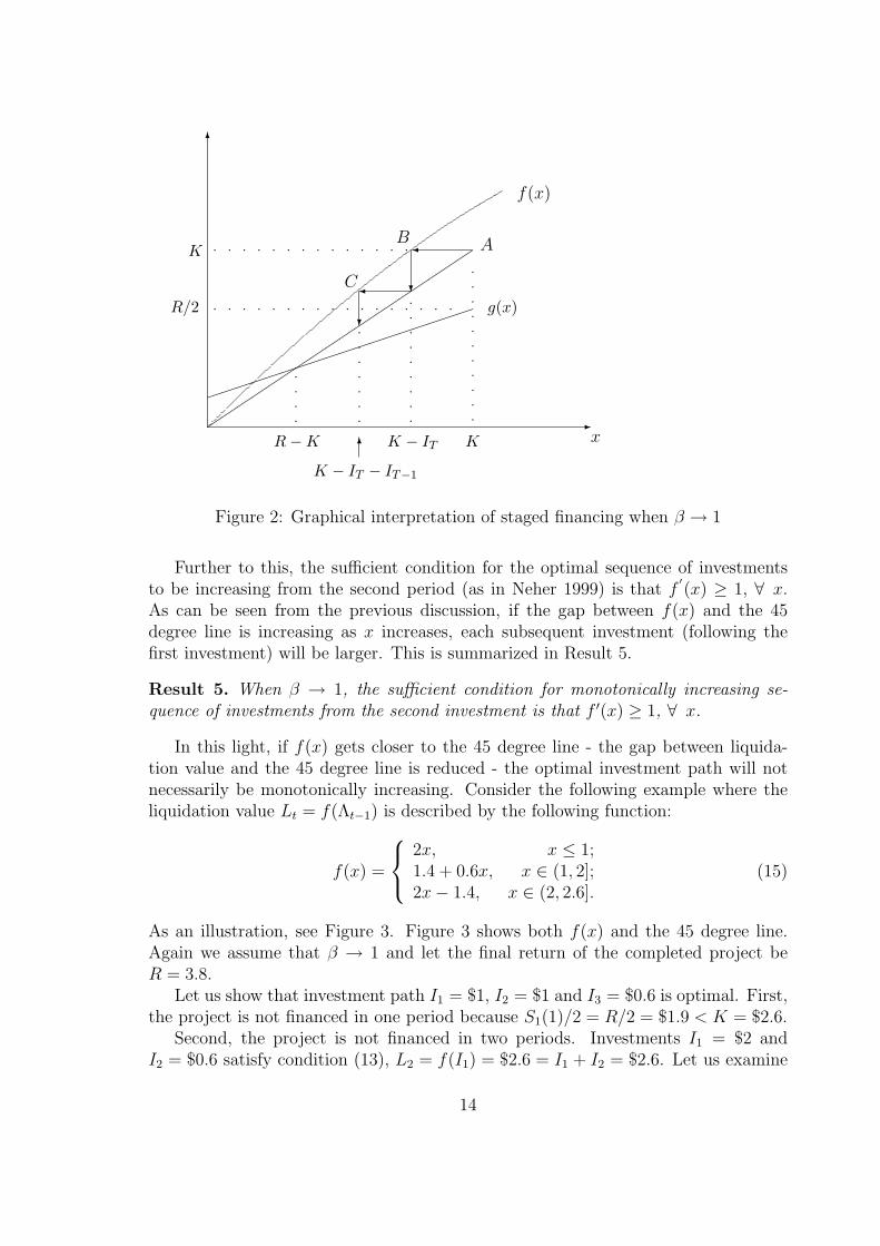
its return R has to be higher than 2K (condition 12). If this is not satisfied consider,as specified by the Algorithm, whether the project can be financed in two periods.From equation 13 when β → 1, the investment in the last (T -th) period has theproperty that f(ΛT−1) = K. We take a point with coordinates (K, K) on the 45degree line (labeled as point A) and draw a horizontal segment until it intersects withf(x) function; label this point B. The distance between A and B is the investmentin the final period for any T ≥ 2. Let us check whether the project can be completedin two periods (T = 2). Investment in the first period in that case would haveto be equal to the horizontal distance between the origin and B; the second-periodinvestment is the distance between B and A. Consider g(x) - the value of S1/2 - whenx = I1 = K − IT . In order for the project to be completed in two periods, g(K − IT )needs to be above the 45 degree line (condition 12). If this condition is not met,we continue the process for three investment periods as specified in the Algorithm.For instance, with three investment periods, from condition 13, the investment in thefinal period is the distance between B and A; the second period investment is thehorizontal distance between C and B; and the investment in the first period is thehorizontal distance between the origin and point C. The project can be financed inthree periods if g(I1) = g(K − IT − IT−1) is above the 45 degree line. If g(I1) liesbelow the 45 degree line, the project cannot be financed in three periods, we continuethe process for four periods, and so on, as specified by the Algorithm.

As shown graphically in Figure 2, the investment required in each period canbe determined moving in a cobweb manner starting at point A so as to measure thehorizontal distance between f(x) and the 45 degree line for each successive investmentuntil we reach a point where condition 12 is satisfied; this will occur when x < R−K.From this we can find the condition when the Algorithm cannot provide a solution tothe problem. This will occur when the cobweb never reaches a point where x < R−K.This will happen when f(x) < x for some x > R −K. In this case the cobweb willconverge to some point x > R−K.9 This discussion is summarized in Result 4.

Result 4. When β → 1 the necessary and sufficient conditions for the project to befinanceable in two or more periods (R > 2K) is that f(x) > x for all R−K ≤ x ≤ K.

This analysis allows us to clearly distinguish between the different roles of thefinal return R and the liquidation value in supporting investment in the project. Theinvestment in the first period is supported by the final return R. Once the projecthas commenced, however, further investments are supported by the liquidation value.Provided the liquidation value is above the 45 degree line - the investor’s collateralexceeds the cost of the investment they have already made - the investor can beassured that repudiation will not occur.

9Note that f(x) - the liquidation value - is a monotonic function. Further, if f(x) is not acontinuous function we amend it by adding vertical segments at the points of discontinuity. Theamended relationship is continuous, which is necessary and sufficient to prove the above claim.

13

-x

6

��

��

��

��

��

��

��

��

��

������������������

f(x)

g(x)

K

R/2

KR−K K − IT

K − IT − IT−1

AB

C

6

ppppppppppp

pppp

ppppppppp

p p p p p p p p p p p p p pp p p p p p p p p p p p p p p p p

ppppppp

�

?�

?

Figure 2: Graphical interpretation of staged financing when β → 1

Further to this, the sufficient condition for the optimal sequence of investmentsto be increasing from the second period (as in Neher 1999) is that f

′(x) ≥ 1, ∀ x.

As can be seen from the previous discussion, if the gap between f(x) and the 45degree line is increasing as x increases, each subsequent investment (following thefirst investment) will be larger. This is summarized in Result 5.

Result 5. When β → 1, the sufficient condition for monotonically increasing se-quence of investments from the second investment is that f ′(x) ≥ 1, ∀ x.

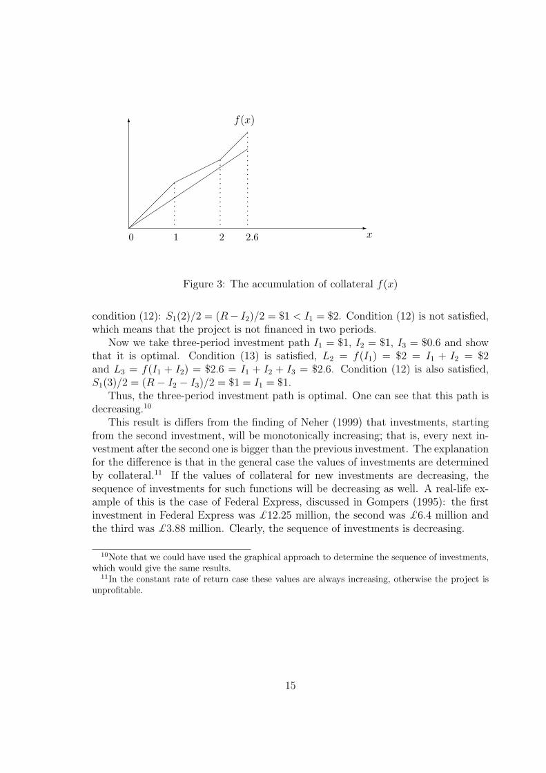
In this light, if f(x) gets closer to the 45 degree line - the gap between liquida-tion value and the 45 degree line is reduced - the optimal investment path will notnecessarily be monotonically increasing. Consider the following example where theliquidation value Lt = f(Λt−1) is described by the following function:

f(x) =

2x, x ≤ 1;1.4 + 0.6x, x ∈ (1, 2];2x− 1.4, x ∈ (2, 2.6].

(15)

As an illustration, see Figure 3. Figure 3 shows both f(x) and the 45 degree line.Again we assume that β → 1 and let the final return of the completed project beR = 3.8.

Let us show that investment path I1 = $1, I2 = $1 and I3 = $0.6 is optimal. First,the project is not financed in one period because S1(1)/2 = R/2 = $1.9 < K = $2.6.

Second, the project is not financed in two periods. Investments I1 = $2 andI2 = $0.6 satisfy condition (13), L2 = f(I1) = $2.6 = I1 + I2 = $2.6. Let us examine

14

-x

6 f(x)

��

��

�

��

��

��

��

��

��

�

������

��

pppppppppp

ppppppppppppppp

ppppppppppppppppppppp

2.61 20

Figure 3: The accumulation of collateral f(x)

condition (12): S1(2)/2 = (R− I2)/2 = $1 < I1 = $2. Condition (12) is not satisfied,which means that the project is not financed in two periods.

Now we take three-period investment path I1 = $1, I2 = $1, I3 = $0.6 and showthat it is optimal. Condition (13) is satisfied, L2 = f(I1) = $2 = I1 + I2 = $2and L3 = f(I1 + I2) = $2.6 = I1 + I2 + I3 = $2.6. Condition (12) is also satisfied,S1(3)/2 = (R− I2 − I3)/2 = $1 = I1 = $1.

Thus, the three-period investment path is optimal. One can see that this path isdecreasing.10

This result is differs from the finding of Neher (1999) that investments, startingfrom the second investment, will be monotonically increasing; that is, every next in-vestment after the second one is bigger than the previous investment. The explanationfor the difference is that in the general case the values of investments are determinedby collateral.11 If the values of collateral for new investments are decreasing, thesequence of investments for such functions will be decreasing as well. A real-life ex-ample of this is the case of Federal Express, discussed in Gompers (1995): the firstinvestment in Federal Express was £12.25 million, the second was £6.4 million andthe third was £3.88 million. Clearly, the sequence of investments is decreasing.

10Note that we could have used the graphical approach to determine the sequence of investments,which would give the same results.

11In the constant rate of return case these values are always increasing, otherwise the project isunprofitable.

15

Appendix

Proof of Proposition 1

The proof consists of two sections. In the first section we only consider investmentpaths that satisfy St ≥ Lt for any t; that is the surplus in any period is at least aslarge as the liquidation value. In the second section we relax this assumption.Section 1To proceed, assume that condition (12) holds and find which path is optimal in thiscase. Here we show that such a path has to satisfy conditions (10), (11) and theMCC.

(12) =⇒ (10)

First, we prove that from condition (12), condition (10) follows. That is, for theminimal feasible T

Lt ≥ St(T )/2 ∀ t = 2, 3, . . . , T.

This statement can be proved by contradiction. Assume that for optimal investmentpath I1, . . . , IT for some t ≥ 2 this property does not hold.12 Let us construct someother shorter path with T ′ = T−t+1, where I ′1 := Λt, I ′2 := It+1,. . ., I ′T−t+1 := IT . Wenow examine whether the feasibility constraints are satisfied for the new path. Thefeasibility constraint (1) is satisfied by construction. Let us prove that the feasibilityconstraint (8) with respect to I ′1 holds, that is I ′1 = I1+. . .+It ≤ S ′

1(T−t+1)/2 = U ′1,

where S ′1(T − t + 1) is a surplus to be bargained over in period one. It is straight

forward to show that this surplus is the same as St(T ) for the initial path. Fromthe assumption that condition (10) does not hold in period t and from the feasibilityconstraint (8) for It it follows that St(T )/2 = Ut ≥ It + . . . + I1/β

t−1 ≥ I1 + . . . + IT .This proves the first feasibility constraint for the new path. If t = T , there is onlyone feasibility constraint, which has just been shown. If t < T , there are some otherfeasibility constraints that need to be considered.

Let us prove that the feasibility constraint with respect to I ′2 holds. We can modifyinequality (8) for period t + 1 to get13

I ′2 = It+1 ≤ Lt+1 − I1/βt − . . .− It/β ≤ Lt+1 − (I1 + . . . + It)/β = L′

2 − I ′1/β.

The same way we prove the feasibility constraint for any I ′i, where 2 ≤ i ≤ T−t+1

I ′i = Ii+t−1 = Li+t−1 − I1/βi+t−2 − . . .− Ii+t−2/β <

< Li+t−1 − (I1 + . . . + It)/βi−1 − It+1/β

i−2 − . . .− Ii+t−2/β == Li+t−1 − I ′1/β

i−1 − I ′2/βi−2 − . . .− I ′i−1/β.

12If there is a set of indexes where condition (10) does not hold then t is the largest index in thisset.

13Note, that in period t + 1 condition (10) holds because t is chosen to be the largest amongindexes for which that condition does not hold.

16

So far we have shown that the constructed T − t + 1 path is feasible. Let usshow the new path allows the entrepreneur to get higher utility than the originalpath. To do this we introduce another T period path, that has zero investmentsduring the first t − 1 periods, and then coincides with the T − t + 1 path, that isI ′′i = 0 ∀ i = 1, . . . , t− 1, I ′′t = I1 + . . . + It, I ′′i = Ii ∀ t + 1 ≤ i ≤ T . Now we showthat this additional T -period path {I ′′i }i=T

i=1 delivers higher utility than the originalT -period path and lower utility than the new (T − t + 1) path, see Figure 4.

I1 I2 It IT

I ′′1 I ′′2 I ′′t I ′′T

I ′1 I ′2 I ′T−t+1

Figure 4: Investment paths {Ii}i=Ti=1 , {I ′′i }i=T

i=1 and {I ′i}i=T−t+1i=1

Comparing the additional and the original paths, both paths generate the samereturn βT R, while the original path has higher costs of delay because some of theinvestments were made earlier. Consequently,

βT R−T∑

t=1

βt−1It ≤ βT R−T∑

t=1

βt−1I ′′t .

The new T -period path is actually T − t + 1-period path that starts after waiting fort− 1 periods. Because of costs of delay the utility from the additional T -period path

17

will be 1/βt−1 smaller than the utility from the T − t + 1-period path

βT R−T∑

t=1

βt−1I ′′t = βt−1(βT−t+1R−T−t+1∑

t=1

βt−1I ′t) ≤ βT−t+1R−T−t+1∑

t=1

βt−1I ′t.

Thus, we have showed that the constructed T − t + 1-period path is both feasibleand delivers higher utility than the optimal T -period path. This is a contradiction.

(12) and (10) =⇒ (11)

Second, we show that condition (11) is also satisfied when conditions (12) and (10)hold. We again prove this statement by contradiction. Assume that for the opti-mal investment path I1, . . . , IT for some t ≥ 2, the following strict inequality holds∑t

i=1 βi−tIi < Ut. To find a contradiction we construct an additional investment pathby moving ε investment from It−1 to It and show that all the feasibility constraintshold and the new path is preferred by the entrepreneur.14

With respect to constraints for periods after t this change is feasible because itonly diminishes the costs of the previous investments. From condition (10) the right-hand side of (8) is Ui = Li ∀ i = 2, . . . , T . These liquidation values are the sameafter the change, while the left-hand sides of (8) diminish because ε investment wasmoved to a later period. Thus after the change the feasibility constraints for periodsafter t are satisfied.

The constraint for t is satisfied because ε is chosen to be small enough.The constraints for periods before t are satisfied because they were satisfied before

the change was made. Both the left- and the right-hand sides of (8) are unchanged.The change is beneficial for the entrepreneur because it only diminishes the costs

of the investment. Thus, this is a contradiction because the original investment pathwas optimal.

(10), (11) and (12) =⇒ MCC

Compare investment path I1, . . . , IT that satisfies conditions (10), (11), (12) and theMCC and some other investment path I ′1, . . . , I

′T that satisfies only (10), (11) and

(12), but does not satisfy the MCC. Let us prove that Λt ≤ Λ′t ∀ t = 1, 2, . . . , T −1.

The inequality for t = 1 follows from the MCC: Λ1 = I1 and I1 is the minimum.The inequality for t = 2, . . . , T − 1 can be proved by contradiction. Assume

Λt > Λ′t for some t = 2, . . . , T − 1. Let us construct some other path {I ′′t }t=T

t=1 thathas Λ′′

t = min[Λt, Λ′t] ∀ t = 2, . . . , T . This path satisfies all the feasibility constraints

because they are satisfied along both original paths. On the other hand, this pathdelivers higher utility than any of {It}t=T

t=1 and {I ′t}t=Tt=1 investment paths because it

14It−1 has to be strictly positive, otherwise the original investment path is not optimal as the(t− 1)-th period can be removed from the investment path.

18

I1 I2 IT

I ′1 I ′2 I ′T

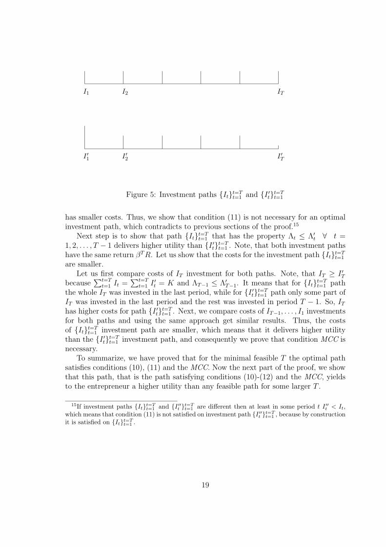
Figure 5: Investment paths {It}t=Tt=1 and {I ′t}t=T

t=1

has smaller costs. Thus, we show that condition (11) is not necessary for an optimalinvestment path, which contradicts to previous sections of the proof.15

Next step is to show that path {It}t=Tt=1 that has the property Λt ≤ Λ′

t ∀ t =1, 2, . . . , T − 1 delivers higher utility than {I ′t}t=T

t=1 . Note, that both investment pathshave the same return βT R. Let us show that the costs for the investment path {It}t=T

t=1

are smaller.Let us first compare costs of IT investment for both paths. Note, that IT ≥ I ′T

because∑t=T

t=1 It =∑t=T

t=1 I ′t = K and ΛT−1 ≤ Λ′T−1. It means that for {It}t=T

t=1 paththe whole IT was invested in the last period, while for {I ′t}t=T

t=1 path only some part ofIT was invested in the last period and the rest was invested in period T − 1. So, IT

has higher costs for path {I ′t}t=Tt=1 . Next, we compare costs of IT−1, . . . , I1 investments

for both paths and using the same approach get similar results. Thus, the costsof {It}t=T

t=1 investment path are smaller, which means that it delivers higher utilitythan the {I ′t}t=T

t=1 investment path, and consequently we prove that condition MCC isnecessary.

To summarize, we have proved that for the minimal feasible T the optimal pathsatisfies conditions (10), (11) and the MCC. Now the next part of the proof, we showthat this path, that is the path satisfying conditions (10)-(12) and the MCC, yieldsto the entrepreneur a higher utility than any feasible path for some larger T .

15If investment paths {It}t=Tt=1 and {I ′′t }t=T

t=1 are different then at least in some period t I ′′t < It,which means that condition (11) is not satisfied on investment path {I ′′t }t=T

t=1 , because by constructionit is satisfied on {It}t=T

t=1 .

19

(10)-(12) and MCC gives higher utility than any path with a greater numberof periods

Consider an investment path that satisfy (10)-(12) and MCC with T periods, namelyI1, . . . , IT , and any other path with T + i periods, namely I ′1, . . . , I

′T+i. Let us show

that the path with T + i during the first i + t periods invests not less than Λt.First, to find a contradiction assume that Λ′

i+1 < I1. Construct another T -periodpath with Λ′′

t = min[Λt, Λ′i+t], ∀ t = 1, . . . , T . Let us prove that this path is feasible.

The feasibility of t = 2, . . . , T constraints follows from the fact that the costs for thenew path are smaller than in any of the two original paths. To prove the feasibilityof the t = 1 constraint rewrite the first feasibility constraint for I1, . . . , IT path in thefollowing way

I1 ≤ βT (R− IT /β − . . .− I2/βT−1 − I1/β

T ).

The first feasibility constraint for the new path is satisfied because I ′′1 < I1 and thecosts for the new path are smaller. Thus, the new path is feasible and it delivers higherutility than the original T -period path, which is optimal among T -period paths. Thisis a contradiction.

Second, to find a contradiction with 2 ≤ t ≤ T assume that Λi+t < It. We use thesame T -period path Λ′′

t = min[Λt, Λ′i+t], ∀ t = 1, . . . , T . We show that the new path

is feasible and delivers higher utility than the original T -period path. This allows usto find a contradiction.

The property Λt ≤ Λ′t+i ensures that the investment path I1, . . . , IT delivers higher

utility than I ′1, . . . , I′T+i. This observation concludes this part of the proof.

Note, that the investment path satisfying conditions (10)-(12) and the MCC isunique by construction.

Property St ≥ Lt,∀ t is satisfied on optimal path

To finish this subsection we prove that St ≥ Lt is always satisfied on the constructedinvestment path. First note that this property holds for t = 1. S1 is positive becausethe project is profitable and L1 = 0 by construction, that is

S1 > L1.

Next, using modified equations (3), (13) and (12) we prove the property holds fort = 2, that is

S2 = S1/β + I2, L2 = I1/β + I2 and I1 ≤ S1/2 =⇒ S2 ≥ L2.

Now, prove by induction that St ≥ Lt. Starting with S2 ≥ L2, as shown above, usingmodified equations (3) and (13) it follows that

St = St−1/β + It, Lt = Lt−1/β + It =⇒ St ≥ Lt ∀ t = 3, . . . , T.

Section 2

20

Here we show that any incentive-compatible path for which the property St ≥ Lt forall t is not satisfied is either: dominated by the optimal investment path derived bythe algorithm; or delivers the entrepreneur negative payoff and, consequently, it willnot be chosen.

Consider an investment path that has

St < Lt

for some 2 ≤ t ≤ T . Let us prove that in that period condition (8) is satisfied.To prove this inequality we use the fact that the project delivers the entrepreneur apositive return, that is

βT R−i=T∑i=1

βi−1Ii > 0.

We divide the inequality above by βt−1 and using equation (3) derive

St >t∑

i=1

βi−tIi.

Combining this inequality with the assumption that Lt > St, we prove condition (8)for period t. It means that in all periods where Lt > St condition (8) is satisfied. Inother periods it is also satisfied because the investment path is incentive compatible.This means that the investment path is feasible for optimization problem (9). Onceit is feasible it is dominated by the optimal investment path constructed by theAlgorithm.

Proof of Result 1

To prove Result 1 we use the fact that on the optimal path St ≥ Lt is satisfied forperiod T . From equation (3) it follows that

ST = βR

and from equation (13)

LT =t=T∑t=1

βt−T It.

Multiply St ≥ Lt by βT−1 we get

βT R−T∑

t=1

βt−1It ≥ 0;

this means that the optimal path constructed by the Algorithm delivers a positivefinal return to the entrepreneur.

21

References

[1] Admati, A. and M. Perry 1991, ‘Joint Projects Without Commitment’, Reviewof Economic Studies, vol. 58, no. 2, pp. 259-76.

[2] Admati, A. and P. Pfleiderer 1994, ‘Robust Financial Contracting and the Roleof Venture Capitalists’, The Journal of Finance, vol. 49, pp. 371-402.

[3] Bolton, P. and D. Scharfstein 1990, ‘A Theory of Predation Based on AgencyProblems in Financial Contracting’, American Economic Review, vol. 80, no. 1,pp. 93-106.

[4] Chiu, S. 1998, ‘Noncooperative Bargaining, Hostages, and Optimal Asset Own-ership’, American Economic Review, vol. 88, no. 4, pp. 882-901.

[5] Gompers, P. A. 1995, ‘Optimal Investment, Monitoring, and the Staging of Ven-ture Capital’, Journal of Finance, vol. 50, pp. 1461-1489.

[6] Hart, O. and J. Moore 1994, ‘A Theory of Debt Based on Inalienable HumanCapital’, Quarterly Journal of Economics, vol. 109, no. 4, pp. 841-79.

[7] Neher, D. 1999, ‘Staged Financing: An Agency Perspective’, Review of EconomicStudies, vol. 66, no. 2, pp. 255-74.

[8] Roberts, K. and M. Weitzman 1981, ‘Funding Criteria for Research, Developmentand Exploration Projects’, Econometrica, vol. 49, pp. 1261-1268.

[9] Sahlman, W. A. 1988, ‘Aspects of Financial Contracting in Venture Capital’,Journal of Applied Corporate Finance, vol. 1, pp. 23-36.

[10] Sahlman, W. A. 1990, ‘The Structure of Governance of Venture-Capital Organi-zations’, Journal of Financial Economics, vol. 27, pp. 473-521.

[11] Shaked, A. and Sutton, J. 1984, ‘Involuntary Unemployment as a Perfect Equi-librium in a Bargaining Model’, Econometrica, vol. 52, no. 6, pp. 1351-64.

22