Staff Papers Series

P80-11 my 1980

RELATIVE PRICES, TECHNOLOGY, AND FARM SIZE

Yoav Ki.slevand Willis Peterson

lDepartment of Agriculturaland AppliedEconomicalL 4

University of Minnesottt

instituteof Agriculture, Forpstry and Home Economics

St. Paul. Minnesota 55108

May 1980

RELATIVE PRICES, TECI-fNOLOGY,AND FARM SIZE

Yoav Kislev and Willis Peterson*

By all conventional measures, average farm size in the United

States has grown substantially over the past half century. From 1930

to 1980 land area per farm increased over 2.5 times while real value

added grew over four-fold. At the same time the number of farms decreased

from 6.3 million to approximately 2.7 million.

The main purpose of this paper is to construct a theoretical

framework which explains the growth in size of full-time family farms.

In the last section of the paper we present empirical evidence which

bears on this hypothesis.

Although the large non-family corporate farms have received much

attention of late, American agriculture still consists mainly of

family farms. As of 1979 only 2.4 percent of all farm and ranch land

in the U.S. was cultivated by non-family corporate farms (USDA, 1979c).L’

In the corn belt this figure was only 1.0 percent. A more significant

trend is the growth in part-time farming. By the late 1970s income of

farm families from off-farm sources exceeded net income from farming

(USDA, 1979a). While part-time farming is not a part of our model, it

will be clear that this phenomenon is closely related to the growth in

the size of full-time family farms.

The out-migration of farm labor and the growth of farm size are two

.aspects of the same economic process. The rise in urban incomes serves

as an incentive for people to leave agriculture. The remaining land is

divided up among fewer but larger farms who arf,able to maintain income

parity with urban people by increasing the quantity of resources at

their command. While changes in the farm labor force are generally

-2-

2/attributed to income equilibrating forces,— the growth in the size of

farm is commonly attributed to economies of scale (Ball and Heady 1972;

Jensen 1977; Gardner and Pope 1978; Hall and LeVeen 1978). Perhaps the

difference in the explanations stems from a separation of the issues.

The out-migration of farm labor is seen as part of the process of

adjustment of the industry, while the farm size issue relates to the

scale of the typical firm. We attempt to explain firm size but in

American agriculture, these two issues cannot be separated. As will be

documented later in the paper, the real quantity of labor per farm in

the United States has remained relatively constant over the past half

century. Therefore the factors that affected the capital/labor ratio in

the industry also has affected the amount of resources per farm, i.e.,

farm size.

There are several analytical difficulties with the concept of

economies of scale, and the way it is advanced to explain farm growth.

Perhaps the most important are that it implies disequilibrium, returns

to scale should vanish once farms reach optimum size, and like

technological change, the concept defines, not explains, the phenomena

of interest. Also, as we detail in Section 7 below, the empirical

evidence does not support unequivocally the existence of the kind of

scale economies that can cause persistent growth for decades.

As an alternative explanation we suggest an equilibrium theory

of the size of the family farm in which three factors play the leading

roles: technology, input prices and non-farm income. We concentrate

on the last two since their introduction constitutes the major

innovation of the paper. The analysis is comparative static in nature

and dynamic adjustments are mentioned only in passing. The paper is

-3-

based on a set of restrictive assumptions formulated to capture the

crucial features of the family farm and to highlight the major

determinants of its size, the most specific of which is the assumption

of exclusive employment of a fixed quantity of

hands or part-time off-farm employment are not

family labor -- hired

considered at this stage,

The analysis pertains to a relatively small farm sector -- urban wages

and factor prices are determined exogenously to the sector. Other

assumptions are formulated in the introductory sections of the analysis;

some of them will be modified in the empirical section at the end of

the paper.

For convenience and ease of exposition the discussion is conducted

in terms of a field-crop farm, but, as explained in Section 7, the

theory applies also to a livestock farm with animals (cows, hogs,

layers) replacing land area. All symbols are redefined in Table 1 and

the analysis is summarized in Table 2. The reader may find occasional

reference to these tables helpful in going through the argument.

1. Scale and innovations

Simplifying,we adopt the number of acres as a measure of farm

size (number of animal units for livestock farms). We assume that

each farm is operated by one full-time farmer with no hired help. With

a single operator, capital deepening -- the increase of capital-kabor

ratio -- takes the form of larger and more powerful machines. There

are two sources for the increased size. Partly it reflects technological

-change, the creation of new knowledge, in the machine producing industry.

In other cases the knowledge to build farm machinery and structures of

various dimensions is readily available and the actual size is determined

by economic considerations -- manufactures design and produce larger

-4-

Table 1: Glossary of Symbols

Variables

Labor

Machinery

Biological inputs

Land

Food (agriculturalproduct)

Rate of interest

Shadow price of mechanical services

Labor machinery price ratio

Technology parameter

Elasticities

Demand for food

Substitution in production between land and

biological inputs

Demand for land as a function (cross) of v

Combined variables

B/A

Machine land ratio (constant)

Augmented land(Land with its machine services)

Share of biological input in output

Functions

Mechanical subprocess

Biological subprocess

Production as a function of A and B

Intensive form of H( )

Marginal products in the mechanical

subprocess (i=K,L)

Quantityper Farm

L (=1)

K

B

A

Y

u

cA/v

b

m

A*

‘B

fm( )

‘b( )

H()

h( )

fmi

Price

w

u

v

P

P

r

qm

ld

-5-

machines as demand arises. In fact, large

bottom ploughs already at the beginning of

tractors were pulling multi-

the century in the “Bonanza

farms” of North Dakota (Drache, 1964) and the same companies that produced

the modest-sized 18-50 hp farm tractors had already in the 1930’s

produced earth moving equipment of very different orders of magnitude.

‘!%uswe view innovations in machine size to be induced by factor .

prices. On this point we accept the perspective of the induced innovation

hypothesis (Hayami and Ruttan, 1971) but unlike that perspective we take

technical change, associated with the creation of new knowledge on the

farm or in the input supplying industries, to be exogenous to agriculture.

The possibility that factor prices affect the direction of technical

change is, for simplicity and in order to focus on the main theme of the

analysis, not

2. The Model

Only one

produced in a

the second is

considered.

agricultural product is produced, call it food. It iS

two-process production function. The first is mechanical,

biological, Both subprocesses exhibit constant returns

to scale, both are essential to production, and there is no substitution

3/between them.– Per-farm output of food, Y, is given by equation (l).

(1) y= f(fm(K,L), fb(A,B))

K capital

L(=l) labor

A land

B biological inputs

fm, fb mechanical and biological subprocesses.

-6-

Although the mechanical and biological subprocesses occur

simultaneously, it will be useful to view production as if it were

conducted in successive steps. In the mechanical subprocess, fm,

capital and labor are combined in the usual continuous fashion to

create units of mechanical services -- call these units mechans.

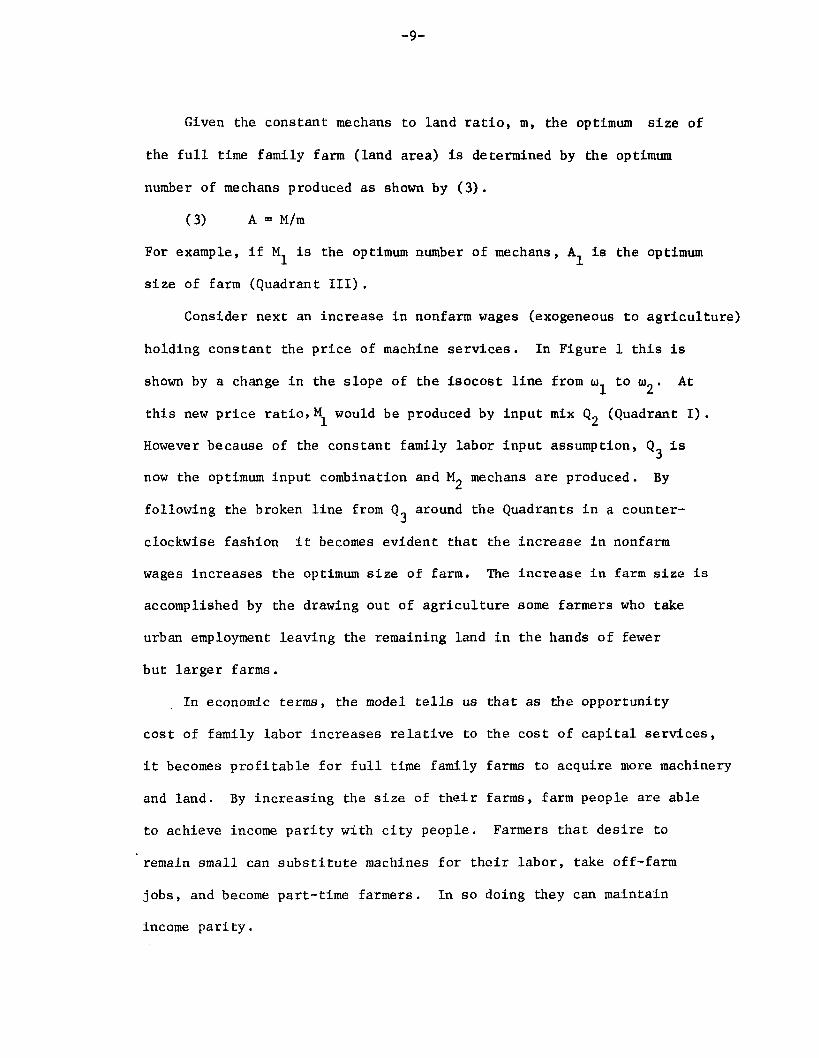
Quadrant I in Figure 1 depicts isoproduct curves of mechans.~’

The assumption of a fixed quantity of family labor per farm is

expressed in the diagram by the vertical line at L = 1.

In Quadrant II we illustrate the production of mechans as a

function of capital for the given one unit input of labor. Note

particularly the assumption of diminishing returns to capital which

implies increasing costs of mechanical services as the capital/labor

ratio rises.

Quadrant III represents the second part of the mechanical subprocess.

In this activity mechans and raw land are combined in fixed proportions

to produce “augmented land.” This is land endowed with the required

amount of mechanical services, call it A*. The constant mechans to

raw land ratio is given by “m”. We assume that this ratio does not

change with the level of biological inputs or with crop yields, i.e.

it takes the same amount of mechanical services to spread a small or

large amount of fertilizer or to harvest a field with a high or low

yield.

In the biological subprocesses,augmented land (A*) is combined

with biological inputs such as feed, fertilizer, herbicides, water, etc.

to produce food. No restriction is placed on the elasticity of substitution

between A* and biological inputs.

-7-

11

‘A”Sfi”;fi

machines

0—- -‘2

I

I

I I

~[

mechans ‘2 ‘1m

It

‘1

●✎

“*‘2

111

land

ti

-- _\

1

/

‘2

‘2

--- -

‘1--- ---

5

\\M2

1

labor

I -S2

I

IV

Figure 1 : The mechanical subprocess of production and the

determination of farm size.

-8-

To reflect production by subprocesses, (1) can be rewritten in a

hierarchical form:

(l’) y = f(fb(A,B,fm(K,L))

= H(A*,B)

where H( ) is the biological subprocess. In the intensive form, food

per

3.

the

acre is

YK* = h(B/A*)

Determination of farm size.

Since each acre of raw land requires m units of mechanical services,

size of the full-time family farm is determined by the number of

mechans produced. The number of mechans is determined in the “mechanical

services department” of the farm, with the production function fm( ), in

the following way. Farmers consider the urban wage as the opportunity

cost of their own labor. Given this wage, w, and the cost of machine

services, u, a farmer will settle at a point of tangency of the factor

price ratio, u, and the M isoquant.

In Figure 1, Quadrant 1, Q1 is the point of tangency for a farm

operated by one family (L=l) facing a price ratio of u .1

In this case

the farmer would hire K1 units of machine services and produce Ml units

of mechans. At any other capital/labor ratio the family farm would not

be minimizing costs while using its full complement of labor. As long

as the individual farm is in business, profits will be maximized only

if the family labor is fully employed. Hence Q1 represents a profit

maximizing as well as a cost minimizing point for price ratio WI.

-9-

Given the constant mechans to land ratio, m, the optimum size of

the full time family farm (land area) is determined by the optimum

number of mechans produced as shown by (3).

(3) A=M/m

For example, if Ml is the optimum number of mechans, Al is the optimum

size of farm (Quadrant 111).

Consider next an increase in nonfarm wages (exogenous to agriculture)

holding constant the price of machine services. In Figure 1 this is

shown by a change in the slope of the isocost line from (AI1to U2. At

this new price ratio,M1 would be produced by input mix Q2 (Quadrant 1),

However because of the constant family labor input assumption, Q3 is

now the optimum input combination and M mechans are produced. By2

following the broken line from Qa around the Quadrants in a counter-J

clockwise fashion it becomes evident that the

wages increases the optimum size of farm. The

accomplished by the drawing out of agriculture

urban employment leaving the remaining land in

but larger farms.

increase in nonfarm

increase in farm size is

some farmers who take

the hands of fewer

,,In economic terms, the model tells us that as the opportunity

cost of family labor increases relative to the cost of capital services,

it becomes profitable for full time family farms to acquire more machinery

and land. By increasing the size of their farms, farm people are able

to achieve income parity with city people. Farmers that desire to

remain small can substitute machines for their labor, take off-farm

jobs, and become part-time farmers. In so doing they can maintain

income parity.

-1o-

4. Land Values

Because of the interrelationshipbetween agricultural prices and

land values, it will be useful at this point to consider how land prices

are determined by the model. Because of the assumption of a fixed

supply of agricultural land which has no alternative use, the return

per acre, p, is a residual

(4) p = (Py-uK-w-vB)/A

The price of an acre is p/r, where r is the rate of interest.

What happens to the price of land when urban wage rates increase?

Because of the higher price of labor and the reduction in the marginal

productivity of capital as more capital is added per unit of labor

(Quadrant II), the costp er mechan at Q3 is higher than the cost at

Q1 ●Due to the assumption of a fixed number of mechans per acre, the

residual return to land is lower at the new, higher wage rate.

Therefore the rental value of

implicit cost of land exactly

producing mechans.

land declines. The reduction in the

compensates for the increased cost of

As long as rent is positive at the new equilibrium, Q3, the increase

in the opportunity cost of farm labor which entails a reduction in the

number of farmers, an increase in capital per unit of labor, and an

increase in farm size, does not effect the supply of food. The reason

is that these changes do not affect the optimal level of biological

inputs, and therefore yield per acre remains constant. Mechans are

produced in a more capital intensive way but the same quantity of mechanical

services (plowing, planting, harvesting, etc.)are performed.

-11-

Up to this point we have assumed that all land is cultivated

and rent is positive. Another situation, which we term the zero rent

case, can occur. Depending on the level of demand for food, factor costs,

and productivity, the cost of production may be higher than the food

price when all agricultural land is cultivated. Were such a situation

to materialize, farmers will find that even with an imputed rental value

of zero, their labor earnings fall short of their opportunity cost, w.

Equilibrium in such a case will be achieved with some land uncultivated.

The equilibrium number of farms will be that number that will fix supply,

and hence food price, at a level that will set p in equation (4) equal

to zero.

Of course, urban wages can increase to the level that will invoke

the zero rent case. In this case the increase in the opportunity cost

of farm labor will reduce the number of farms, total cultivated acreage,

and the supply

food increases

is achieved.

of food. Food supply will decline until the price of

to the point where zero rent prevails and equilibrium

5. Price Changes

a. Labor. In

an increase in the

the two preceding sections we demonstrated

opportunity cost of farm labor (urban wage

that

rates)

will increase the optimum size of farms, reduce the rental value of

farm land, and may or may not change the supply of food depending on

whether the year rent case is encountered.

In Figure 1 the capital-labor substitution phenomenon is

presented in terms of the individual farm. As farms become larger they

move to higher and higher isoquants,M1toM2, etc. For the agricultural

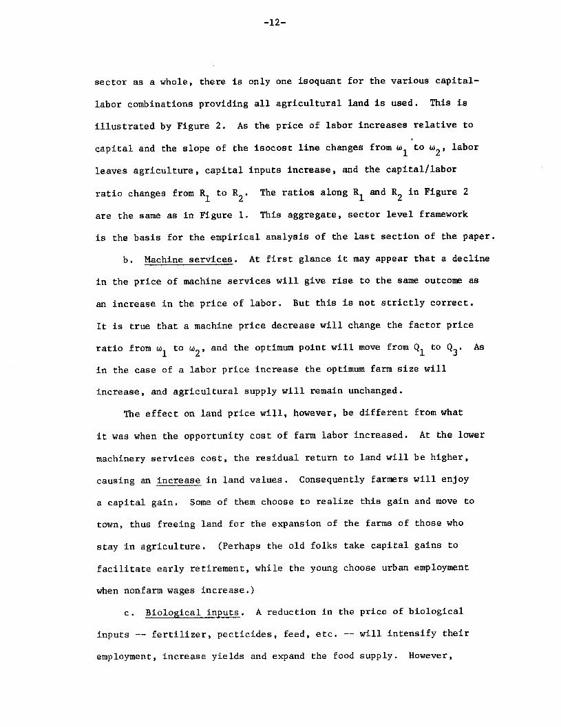
-12-

sector as a whole, there is only

labor combinations providing all

illustrated by Figure 2. As the

one isoquant for the various capital-

agricultural land is used. This is

price of labor increases relative to9

capital and the slope of the isocost line changes from u1to U2, labor

leaves agriculture, capital inputs increase, and the capital/labor

ratio changes from R1toR.

2The ratios along RI and R2 in Figure 2

are the same as in Figure 1. This aggregate, sector level framework

is the basis for the empirical analysis of the last section of the paper.

b. Machine services. At first glance it may appear that a decline

in the price of machine services will give rise to the same outcome as

an increase in the price of labor. But this is not strictly correct.

It is true

ratio from

that a machine price decrease will change

w, to u,, and the optimum point will moveJ- .4

the factor price

from Ql to Q3. As

in the case of a labor price increase the optimum farm size will

increase, and agricultural supply will remain unchanged.

The effect on land price will, however, be different from what

it was when the opportunity cost of farm labor increased. At the lower

machinery services cost, the residual return to land will be higher,

causing an increase in land values. Consequently farmers will enjoy

a capital gain. Some of them choose to realize this gain and move to

town, thus freeing land for the expansion of the farms of those who

stay in agriculture. (Perhaps the old folks take capital gains to

facilitate early retirement, while the young choose urban employment

when nonfarm wages increase.)

c. Biological inputs. A reduction in the

inputs -- fertilizer, pesticides, feed, etc. --

employment, increase yields and expand the food

price of biological

will intensify their

supply. However,

capital

‘2

K1

labor

‘2 ‘1

Figure 2: The agricultural sector.

-14-

because of the non-substitutability assumption between mechans and land

in the production function, the decrease in the price of biological

inputs will not affect the capital/labor ratio and farm size.

On the other hand, the decrease in the prices of the biological

inputs will affect land values. The increased use of these inputs will

I increase the marginal product of land. At the same time, the increase

in the supply of food causes

an opposite influence on the

To analyze the relation

a decrease in its price, thereby having

demand for land.

between biological input prices and land

values, let o be the elasticity of substitution between A and B in

K( ) of equation l’), n the absolute value of the demand for food, and

‘B= vB/PY, the share of biological inputs in total output. Then the

elasticity of demand for land with respect to biological input prices,

‘A/v‘is (Ferguson, Ch. 12)

(5)‘A/v

= SB(CW)

Accordingly the demand for land and land prices will increase in

response to a decline in v if a < n, and decline if u > n.

As in the case of an increase in nonfarm wages, the demand for land

can decrease to the point where the zero rent case prevails and some

land goes unused. Even in this case, however, the use of biological

inputs, both per acre and in the aggregate, will increase; otherwise

supply will not expand and food price will not decline.

d. Food. In order to more clearly see the process of adjustment,

we begin at the zero rent case where some land is uncultivated. Assume

the demand for food increases. 1P the short run the price of food will

increase temporarily, resulting in a capital gain to farmers, and serving

-15-

to draw more farmers into agriculture. However, in the long run, as

long as some land remains uncultivated, equilibrium food price will not

change. Further increases in the demand for food eventually will be

met by the land constraint. Now food price will increase in the long

run as will the price of land. Because farmers enjoy a capital gain

their total income, rW + u, will rise but the opportunity cost of their

labor will remain at parity with urban earnings. After the land

constraint is encountered the total quantity of food supplied will

increase because of the increased demand for and use of biological

inputs. But farm size will increase only if the opportunity cost of

farm labor (nonfarm earnings) increases relative to the price of

capital services.

6. Technological Change.

Traditionally technological change has been described by shifts

in a production function or the respective isoquants.

as the basic laws of physics, biology, chemistry etc.,

there can be no increase in output without an increase

However as long

remain unchanged,

in inputs.

Therefore shifts in a production function can occur only if inputs

increase in quality and their measurements do not fully reflect this

quality, or if new inputs which come on the scene are omitted from the

production function. However the improved inputs will not be adopted

unless their real prices are lower than the inputs they replaced~ or

in the case of new inputs, unless their VMPS exceed their prices.

Thus one can analyze technological change either in terms of shifts

in a production function where inputs are not adjusted for quality or

measured correctly, or in terms of lower input prices with the inputs

-16-

adjusted for quality changes. The results should come out the same.

a. Mechanical. Because neutral or non-neutral shifts in isoquants

are a common way of depicting technological change, we shall run these

shifts through the model and observe the consequences. Consider first

a neutral technological improvement in the production of mechanical

services, fm( ) in equation (1). Graphically, the isoproduct curves

in Figure 1 shift toward the origin. Then, say, the curve labelled Ml

becomes M2 after the shift. Also the production function in Quadrant II

shifts up and to the left. Since the shift is neutral and the slopes

of the isoproduct curves along the rays from the origin do not change

Q, will still be the optimum combination. Hence a neutral shift inJ.

the production function of mechanical services will

(fromMl/m to M2/m) without increasing the~

used.

increase farm size

amount of machines

Of course, if the machines were adjusted for quality, total machine

use would increase because higher quality machines are more machines than

than those of lower quality. In this case the real price of machine

services would have declined, providing they were adopted, and the

same result obtained as in section 5b above.

is

of

The conventional case of machine biased technological change in fm

depicted in Figure 3. Again this assumes that the quantity and price

the machines have not been adjusted for quality changes. The

isoquant Ml becomes ~1 and the price ratio Ml which was tangent to Ml

at Q1 is now tangent to ~1 at Q2, Equilibrium along the L=l line will

now be at Q3 and optimum farm size will increase. Unlike the previous

case of neutral technological change in fm~ the measured amount of

machines now increases. In constant quality units the increase in

machine use would be greater here than in the previous case because of

-17-

K(machines

L=l(labo~ers)

Figure 3: Biased technological change in the mechanical service sector.

-18-

the increased MPP of machines vis-a-vis labor. In both the neutral

and non-neutral shifts, the level of biological inputs is not affected

leaving food supply and food prices unchanged. Because of the

assumptions underlying the model, the lower production costs (reduction

in the real price of machine services) are reflected in larger residual

returns to land and higher land values.

b. Biological. Consider a neutral technical change in fb, that

is,in H ( ), with a technology parameter, A,

(10) y = AH(A, B)

An increase in A will increase yield and supply of food. It will also

reduce the price of food. To analyze the demand for B and the returns

to land, note that value of marginal product of an input changes with

technology according to

(11) & (PAHi) = PHi(l - l/n) i =A, B

Therefore, if the demand for food is inelastic, neutral technological

change in the biological sub-process will call forth a decrease in

the amounts of the factors of production; that is, it will entail

a decrease in the use of biological inputs, measured without equality

adjustments, and lower land values. The opposite will be true if

demand is elastic.

If the agricultural sector were to acquire both land services and

the factor B on the free market at fixed prices, then (since technological

change is assumed neutral), the use of both factors would have contracted

or expanded proportionally. With land in fixed supply and being the

residual rent receiving factor, the quantitative change in the employment

of the biological factors depends on the elasticity of substitution in

H().

-19-

00

.

-t -t 00 .+ I

+--t o c) + o

wo

I + I -1- +-++1

CJo I 00 I

G.F+

uCJ

to

(30 ++o 0

I I I I o alL1‘m

+j’

314

:.rl

+ + + -t- C3

,....A

t-l

cv

c1

,.8

l+

v,:.

U-Ja

T{.fs

/---0.:1

L,

CJ .G

....i

.’=

i%G

C’.J.I-lnaJ

<-’(,,f;

;1

-20-

Biological technological change will not change farm size. It may,

though, tilt the economy over to the zero rent case with idle land,

zero rent and a smaller number of farms than the one prevailing before

the

7.

change.

Other Issues

a. Livestock. Livestock share with field crops the same general

features of the production process: mechanical services are proportional

to the size of the enterprise and virtually unaffected by yield (milk

per cow, eggs per layer, feed conversion ratios in meat animals and

poultry, etc.). Once the appropriate mechanical services have been

provided, the yield per unit of livestock is determined by biological

factors including inputs such as feed, medicine, and genetic material.

The dual process production function of equation (1) can be applied

without modification, where A now represents number of livestock units

and B is mainly feed. The previous analysis of the size of farms and

intensity of utilization of biological inputs can be applied equally to

livestock farms and field crop operations.

There is however one difference between the two types of farms.

Because no factor is in fixed supply in the livestock case, there is

no residual receiver of rent. Therefore the zero rent case applies,

except in the short run situation of a growing livestock industry

where the rate of growth is constrained by the size of the breeding

herd. In this case rent to breeding stock capital could be positive.

The optimal size of the livestock farm also is determined by the

process depicted by Figure 1. In equilibrium the number of farms will

be such that the supply forthcoming together with demand will set a

-21-

price of the product that will equate costs and returns in the industry.

In other words, one can view labor as the residual income receiver,

and the number of livestock farms will be such that on-farm labor

earnings will be equal to the urban wage rate.

A significant share of livestock production in the U.S. is on

diversified farms, typically on farms combining a field crop and a

livestock enterprise. Virtually all hogs and dairy cows in the Midwest

and in the East and a substantial share of beef fattening are done on

farms that produce their own fee~. However, poultry almost everywhere

and dairy farms in the Southwest and West are usually completely

specialized. In the past, diversificationwas more pronounced than

today and was probably practiced mainly in order to reduce risk and

to assure a home supply of livestock products. In a modern, market-

oriented agriculture, the main advantage of on-farm production of feed

lies in the elimination of cost of handling, marketing and transportation

between the field crop and the livestock farmers. For diversified

farms, machinery such as grain elevators, silo unloaders, milking

machines, and manure disposal equipment play a similar role in livestock

production to the one played by tractors and equipment in field crop

operations. For the discussion of farm size one can, therefore, assume

that field crops and livestock enterprises grow proportionally. The

question of the determinants of optimal enterprise combination lies

outside the scope of this paper.

b. Economies of Scale. The analysis in this paper has demonstrated

that growth in farm size can be explained without reference to the catch-all

-22-

“economies of scale”. However, such economies are also not so clearly

supported by the empirical record, at least as we read it. True, some

of the ordinary least square estimates of Cobb-Douglas production

functions have yielded high scale coefficients. Griliches (1964), for

example, reported sums of elasticities for an aggregate, state level

production function in the range of 1.2 to 1.3. However, other,

particularly farm level estimates, indicated decreasing returns (Kislev

1966; Hoch 1976). Moreover OLS estimates can be criticized as being

biased upward due to the omission of a management factor which is

positively correlated with size of operation (Mundlak 1961). Indeed,

covariance analysis with a firm effect accounting for management, yields,

in most cases, decreasing returns even in samples which OLS estimates

indicate strong economies of scale (Hoch 1976).

A possible explanation for the difference in results is the age

distribution phenomenon. The inclusion in the same sample of young

(and old) farmers having comparatively small operations and inefficient

asset combinations together with well established farmers in their

prime age and balanced asset structure, will result in upward biased

OLS estimates of returns to scale. Such bias is eliminated with

covariance analysis.

Other evidence, coming from synthetic “engineering” firm analysis,

have indicated eocnomies of scale that are sharply reduced once the

size of a one or two-man operation is reached (Madden and Partenheimer

1972; Hall and LeVeen 1978). The significant aspect of those findings

for the explanation of the historical growth in farm-size is not the

mere existence of scale economies at the family-farm range of operation,

but rather the persistent upward shifts of optimum size often found in

-23-

cost analyses and attributed to the market appearance of new machines

(Rodewald and Folwell 1977), There is, however, an identification

problem here. Undoubtedly, new machines reflect, in part, new

exogenous technological developments which reduce the real cost of

mechanical services and induce growth in farm size. Partly, however,

they also reflect endogenous changes in equipment needed to adopt

production to a rising opportunity cost of farm labor. Attributing

all growth in farm size to exogenous technological developments clearly

overstates the effect of this factor.

c. Structure. The structural assumptions on which this paper

rests are of two kinds: (a) the formulation of the theory and its

empirical application in terms of a single product and uniform production

conditions implies that the same economic factors are assumed to similarly

affect growth of farms of different types and regions, (b) the relevancy

of the study depends on the stability and the resiliency of the family

farm. However, the analysis not only relies on the assumption of this

institutional viability, it can also shed explanatory light on the

forces that maintained the industrial organization of American agriculture.

The U.S. farm sector owes it structure to the historical patterns

of settlement and homesteading. Its stability is fostered by strong

economic forces whose operation is best illustratedwith the few episodes

of large scale farming in the mid-west. For example, some of the

Bonanza Farms of the Red River Valley cultivated in the last third of

the 19th century more than 20,000 (one even 55,000) acres (Briggs, 1932;

Drache, 1964) and similar sizes were also reported for Illinois and

Iowa (Gates, 1932). These huge enterprises, that depended on a large

-24-

hired labor force and substantial investment in power and equipment

ceased to operate and were sold, subdivided into family units, at the

beginning of this century.

The dominance of the family unit in agriculture and of the large

corporation in the nonfarm sector testify to the lack of significant

economies of scale in farming and to their existence in other industries.

Owners of large amounts of wealth will, therefore, invest their

in the nonfarm sector. If, in addition, large farm enterprises

into scale diseconomies, such large holdings will be subdivided

family units. Thus, the American family farm was preserved by

non-farm investment opportunities.

capital

run

into

ample

In the less developed countries, on the other hand, where investment

opportunities outside agriculture are less attractive, the rich have

to accumulate their capital in land even if large holdings are comparatively

inefficient (Berry and Cline 1979). This suggests an hypothesis on the

connection between agraian

test of such an hypothesis

study.

6. Empirical Evidence

structure and urban development. The empirical

is, of course, outside the scope of the present

Changes in facor prices change the capital/labor ratio according

to the elasticity of substitution. This explains the growth of

mechanical services and farm size. Biological inputs are not considered

at this stage.

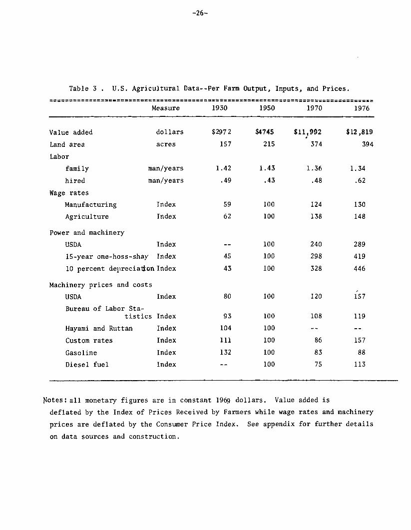
a, Salient features. The major

growth are presented in Table 3. The

size reported below is limited to the

magnitudes associated with farm

empirical analysis of farm

period 1930-1970. Long run

-25-

adjustments to the large price fluctuations of the mid 1970s have yet

to run their course, although data for 1976 are included in the table

to provide an indication of future trends,

Sources and definitions of data are detailed in the Appendix. The

salient features to note in Table 3 are: (1) the substantial growth in

farm size as indicated by the near quadrupling of value added and more

than doubling of acres per farm; (2) the relative constancy of family

and hired labor per farm; (3) the large growth of power and machinery;

(4) the increase in the price of labor relative to machinery.

The labor variable has been adjusted for quality changes

increased educational level of the rural farm population over

due to the

the period,

This quality adjustment increased the per farm family labor input about

20 percent between 1930 and 1970 which serves to offset the 18 percent

reduction in the unadjusted family labor input due to the decline in the

average size of family. ‘IIIUSthe assumption of a constant (quality

adjusted) family labor input appears justified. Real wages in manufacturing

and agriculture, both adjusted for schooling, increase substantially

over the period with the latter closing the gap in more recent years.

Because of the difficulty of measuring quality changes in machinery,

several measures

would argue that

of machine inputs, prices, and costs are presented. We

custom rates provide the most accurate measure of the

real cost of machine services. ~is market determined figure should

reflect reductions

- of improvements in

of capital, mainly

Note that the real

parallel to custom

in the real cost of machine services not only because

quality but also due to the preferential tax treatment

investment credit and accelerated depreciation.

cost of fuel, a major part of machine costs, moves

rates.

-26-

Table 3 . U.S. Agricultural Data--Per Farm Output, Inputs, and Prices.

==================--------------------------------------------------------------------------------------------------------------------------------Measure 1930 1950 1970 1976

Value added dollars $2972

Land area acres 157

Labor

family man/years 1.42

hired man/years .49

Wage rates

Manufacturing Index 59

Agriculture Index 62

Power and machinery

USDA Index --

15-year one-boss-shay Index 45

10 percent de~]reciatimnIndex 43

Machinery prices and costs

USDA

Bureau

Hayami

Custom

Index 80

of Labor Sta-tistics Index 93

and Ruttan Index 104

rates Index 111

Gasoline Index 132

Diesel fuel Index --

$4745

215

1.43

.43

100

100

100

100

100

100

100

100

100

100

100

$11:992

374

1.36

.48

124

138

240

298

328

120

108

---

86

83

75

$12,819

394

1.34

.62

130

148

289

419

446

{57

119

--

157

88

113

~otes: all monetary figures are in constant 1969 dollars, Value

deflated by the Index of Prices Received by Farmers while wage

prices are deflated by the Consumer Price Index. See appendix

on data sources and construction.

added is

rates and machinery

for further details

-27-

The official USDA price index has been criticized for neglecting

to take quality into account (Griliches 1960, and Fettig 1963). As a

result the actual quantity of power and machinery is likely to have

grown more rapidly than the official USDA index indicates. Moreover

the rapid write-off of machinery by farmers makes it appear that the

stock of machinery is smaller than it really is. Our indexes of

machine stocks which were built up from value of shipments data using

alternative 15-year one-boss-shay and constant 10 percent depreciation

assumptions allow for longer life machines. Consequently they show

a substantially larger increase in machinery stocks than the USDA index.

b. Easticity of substitution. h“ empirical test of the model

requires an unbiased estimate of the elasticity of substitution between

capital and labor as well as constant quality measures of inputs and

their respective prices. To incorporate simultaneity in the labor market,

the elasticity of substitution between capital and labor is estimated

in the following two equation model, expressed in logarithms:

(7) y=al+~w+e demand

(8) W=~2+di+~y+E supply

w“ farm wage rate;

Y = value added per unit of labor;

w= manufacturing wage rate;

e,c = independently distributed random disturbance terms.

The demand equation is derived form the CES production function

(Arrow, Chenery,

of farm labor is

nonfarm earnings

Minhas and Solow 1961; Minasian 1961). The supply

influenced by manufacturing wages, w, a proxy for

opportunities, and farm earnings, y.

-28-

The demand equation can be identified and estimated with

manufacturing wages as an Instrumental Variable. In Table 4 we report

the results of these estimates along with OLS estimates of equation (7).

The estimates are cross section for each of the six census years shown,

using states as the unit of observation (n=48, see the Appendix for

details of data construction). To account for differences in size

of states, weighted regressions also

farms in each state as weights.

In general the IV estimates are

are estimated using number of

higher than the OLS figures. All

the IV estimates in the weighted regressions are not significantly

different from 1.8, therefore we use this value for u in the calculations

to follow.

c, Other estimates. Both Griliches (1964) and Binswanger (1974)

reported elasticity estimates that were not significantly different

from 1 which is substantially smaller than our figures. The differences

in the estimates are evidently due to differences in specification, in

particular, Griliches and Binswanger disregarded simultaneity of

urban-rural labor income, grouped several states to single observations,

and did not use weighted regressions. Also Binswanger used a multi-

factor formulation. Low elasticity values are hard to reconcile with

historical developments. By our calculation, the ratio of wage to machiae

costsincreased almost 3 times over the 40 year, 1930-1970 period and

the ratio of machine to labor inputsincreased over the same period by

a factor of more than 6.5. These magnitudes suggest either an elasticity

of substitution which is close to 2 or substantial changes in demand.

Demand for machinery may have increased as a result of the introduction

-29-

Table 4: Elasticity of Substitution

1949

19s4

1959

1964

1969

1974

Notfl?s: a.

b.

c.

Unweighed Regressions Weighted Regressions

OLS

1.48

(7.71)

1.83

(11.16)

1.23

(6,12)

1,13

(4.67)

1,07

(2,30)

1.35

(2.97)

Iv

1.81

(6.81)

1.96

(8,31)

1,65

(5.48)

1.48

(3.47)

1.78

(1.71)

2.10

(1.69)

OLS IV

1.54

(11.00)

1.84

(13.53)

1.33

(7.73)

1,32

(6.35)

1.22

(2,90)

1.23

(2.96)

1,67

(8.03)

1.79

(9.52)

1,47

(5.72)

1.34

(3.82)

1.69

(1,96)

2,16

(1.69)

The estimated equation is (7), number of observations 48.

The figures in parenthesis are t ratios. The t values for IV

regressions are calculated according to Maddalla, 1977, P. 239.

Weighting is by the number of farms in each state for each Year”

-30-

of seasonally sensitive varieties for example, but it is hard to see

how such changes may have doubled the demand for machinery on the

farm, which they should have done to explain the quoted quantitative

relations.

Binswanger used in his study USDA time series data in which the ratio

of machinery service to labor cost rose after the Second World War,

He, therefore, concluded that biased technical change must have been

important in the intensive process of agricultural mechanization. ‘lhitB

conclusion, which runs counter t~ our theoretical assumptions and

interpretation of the data, is, however, unwarranted because Binswanger

did not adjust machinery prices for quality. The quality unadjusted

prices which

react to the

registered increases are economically meaningless; farmers

effective cost of machinery, in standard efficiency units,

Effective cost fell relative to labor cost and mechanization can therefore

be explained as a straightforward reaction to price signals without the

need to suggest biasedness in technical change.

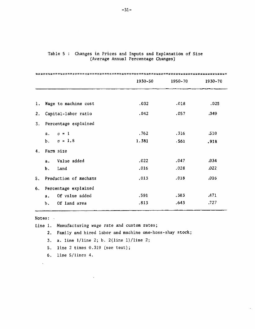
d. Explanation of growth in farm size. The average annual rate

of change over the 40-year-period(1930-70in the ratio of labor to

machine cost was 2.5 percent, while the capital/labor ratio grew at the

rate of 4.9 percent per annum (Table

fore, about half the input change if

5). Price changes explain, there-

the often quoted value of a = 1

is accepted, and 92 percent of the change if a = 1.8 is adopted. If one

accepts 1.8 for the elasticity of substitution, then the “over-explanation”

in the first period (1.381 in line 3b) might be attributed to the

unusual circumstances associated with the Great Depression and the WW 11

years, The 1950-70 period can be looked upon as a time of “catching up”

to the adjustments that would have occurred in the preceding two decades

-31-

Table 5 : Changes in Prices and Inputs and Explanation of Size(Average Annual Percentage Changes)

-------- ------- ---------- -------- ------- -------------- ------- -------- -------- --------- -------------- -------- ---------------------- -------------- ------- ------

1930-50 1950-70 1930-70

1. Wage to machine cost

2. Capital-labor ratio

3. Percentage explained

4. Farm size

a. Value added

b. Land

5. Production of mechans

6. Percentage explained

a. Of value added

b. Of land area

.032

.042

.762

1.381

.022

.016

.013

.591

.813

.018

.057

.316

.561

.047

.028

.018

.383

.643

.025

.049

.510

,918

.034

.022

,016

.471

.727

Notes: ~~

Line 1. Manufacturing wage rate and custom rates;

2. Family and hired labor and machine one-boss-shay stock;

3. a. line I/line 2; b. 2(line 1)/line 2;

5. line 2 times 0.319 (see text];

6. line S/lines 4.

-32-

under more normal circumstances, as well as a time of adjusting to

changing relative price ratios,

Given the stock of capital, farm size is determined by the quantity

of mechanical services (mechans) produced. To gauge changes in this

variable we adopt the production function estimate of Griliches (1964).

His coefficients for labor and machinery were .426 and .200 respectively.

Assume that these coefficients represent the relative elasticities of

labor and machines in the production of mechans and that this subprocess

is subject to constant returns to scale. Then in a linear homogeneous

.200mechans production function the machine coefficient will be

.426 + .200 =

.319. Applying this figure to the growth in power and machinery we

obtain an annual rate of growth, over the 1930-70 period, of the production

of mechanical services of

72.7 percent of growth in

in value added per farm.

1.6 percent (Table 5). This growth explains

land per farm and 47.1 percent of the growth

The difference is probably due to the fact

that growth in value added reflects quality improvements of biological

factors: chemicals, seeds, medicine, etc.

8. Epilogue

Over the 20 year 1950-70 period, the ratio of manufacturing wages

to machine costs (custom rates) increased at a rate of 1.5 per cent

per annum while

per cent (Table

reversed during

land per farm increased at an annual rate of 2.8

3). However the trend in the factor price ratio was

the 1970-76 period when machine costs rose faster than

wages at an annual average rate of about 10 percenti.

The model predicts that the reversal of the capital/labor price

trend should eventually stop the growth in farm size, and perhaps even

-33-

reverse it. It is too early to tell whether this trend will persist,

although it is interesting to note that the annual growth in land area

per farm declined to almost one-third of its previous rate during the

1970-76 period. If the relative

should not be surprised to see a

if the relatively high inflation

growth in energy costs persists, one

decline in farm size. Of course,

rates of the 1970s continue, land

will continue to be an attractive investment, and farm size may grow

for this reason alone. Our model which assumes zero inflation is not

designed to handle the inflation phenomenon. Many interesting questions

remain including the impact of inflation on farm size, the reasons for

the increase in use of biological inputs, the increased popularity of

part-time farming, as well as the explanation for changes in the size

distribution of farms.

9. Summary and Conclusions.

In this paper we have developed an equilibrium theory of optimum

farm size. According to our model, the growth in the size of farms

in the United States has occurred because of the increase in the

opportunity cost of family labor relative to the cost of machine services.

As nonfarm incomes have increased, farm people have attempted to

achieve income parity by increasing the size of their farms. The growth

in farm size was made possible by farmers who left agriculture to

take advantage of higher earnings in the nonfarm sector. The land

which they released has been incorporated into fewer but larger farms.

Moreover, we have explained the growth in farm size without relying

on the “catch-all” phrases of economies of scale and technological

change.

-34-

Footnotes

* Hebrew University, Rehovot, Israel and The University of Minnesota,

St. Paul, Minnesota. We are indebted to Zvi Griliches, Hans

Binswanger and members of seminars at Minnesota, Yale and Rehovot

for comments and suggestions. Most of the work on this study was

done in Minnesota when Yoav Kislev was visiting the Department

Agricultural and Applied Economics. The project was supported

Israel by the United States-Israel Agricultural Research and

Development Fund - BARD.

~/ Of course many family farms have incorporated for tax purposes

of

in

and

to facilitate transfer between generations. “Farming corporations,

like partnerships, tend to be closely held by a few family shareholders.

Eighty percent of privately held farming corporations had five or

fewer shareholders, and 79 percent were family owned, with family

members directly involved in daily operations. Ninety percent of

the closely held corporations had most of their management provided

by shareholders. Farming is the primary, and often the only,

business for these corporations. Corporations are frequently

operated similar to partnerships and often formed to preserve the

family farming operation by facilitating the transfer of assets

between generations.” (USDA, 1979b, p. 8).

~/ While we believe that the opinion in the text is shared by many

economists, we could find no written statement with reference to

American agriculture. For an elaboration in the context of developin~

economies, see Ranis and Fei (1961).

-35-

~/ Linear homogeneity of the mechanical subprocess is not essential;

a homothetic production process will yield identical analytic

results.

~/ We are indebted to John Fei for suggesting the four-quadrant

configuration.

-36-

References

Arrow, K. J., H. B. Chenery, B. S. Minhas, and R. M. Solow, 1961,

“Capital-Labor Substitution and Economic Efficiency,” Review of

Economics and Statistics, 43: 225-250.

Ball, Gordon A,, and Earl 0, Heady, 1972, Size, Structure and Future of

Farms, Iowa State University Press.

Berry, R. Albert and William R. Cline, 1979, Agrarian Structure and

Productivity in Developing Countries, Baltimore and London: Johns

Hopkins University Press.

Binswanger, Hans P., 1974, “The Measurement of Technical Change Biases with

many Factors of Production,” American Economic Review, Dec. 64: 964-76.

Binswanger, Hans P., Vernon W. Ruttan, and others, 1978, Induced

Innovation, Technology, Institutions, and Development, Baltimore

and London: Johns Hopkins.

Briggs, Harold E., 1932, “Early Bonanza Farming in the Red River Valley

of the North,” Agricultural History, 6: 23-37.

Carter, H., and G. Dean, 1961, “Cost-Size Relationship for Cash-Crop

Farms in a Highly CommercializedAgriculture,” Journal of Farm

Economics 43: 264-277.

Drache, Hiram, 1964, The Day of the Bonanza, Fargo: North Dakota

Institute for Regional Studies.

Ferguson, C. E., 1975, The Neoclassical Theory of Production and

Distribution, Cambridge University Press.

Fettig, L. P., 1963, “Adjusting Farm Tractor Prices for Quality Change,

1950-62,” Journal of Farm Economics, 45: 559-611.

-37-

Gardner, B. Delworth and Dulon D.

Determined in Agriculture?”

Economics, 60: 295-302.

Pope, 1978, “How is Scale and Structure

American Journal of Agricultural

Gates, Paul Wallace, 1932, “Large Scale Farming in Illinois, 1850-1870,”

A~ricultural History, 6: 14-25.

Griliches,Zvi, 1960, ‘pleasuringInputs in Agriculture: A Critical

Survey,” Journal of Farm Economics, Dec., 42: 1411-27.

Griliches,Zvi, 1964, “Research Expenditures, Education, and the Aggregate

Agricultural Production Function,” American Economic Review,

54: 961-974.

Griliches, Zvi, 1963, “The Sources of Measured Productivity Growth;

United States Agriculture, 1940-60,” Journal of Political Economy,

71: 331-346.

Hall-; Bruce F. and E. Phillip LeVeen, 1978, “Farm Size and Economic

Efficiency: The Case of California,” American Journal of Agricultural

Economics, 60: 589-600.

Hayami, Y., and V. W. Ruttan, 1971, Agricultural Development: An

International Perspective, Baltimore: The Johns Hopkins Press.

Hoch, Irving, 1976, “Returns to Scale in Farming: Further Evidence,”

American Journal of Farm Economics, 58: 745-49.

Jensen, Harold, 1977, “Farm Management and Production Economics, 1946-70”,

in Lee R. Martin (cd.), A Survey of Agricultural Economics

Literature, Vol. 1, Minneapolis: University of Minnesota Press.

Kislev, Yoav, 1966, “Overestimationof Returns to Scale in Agriculture --

A Case of Synchronized Aggregation,” Journal of Farm Econo~cs,

48: 967-83.

-38-

Kislev, Yoav and Willis Peterson, 1980, “Induced Bias in Technical

Change: A Comment,” mimeo.

Maddala, G. S., 1976, Econometrics, New York: McGraw Hill.

Madden, J. Patrick and Earl J. P~rtenheimer, 1972, “Evidence of Economies

and Diseconomies of Farm Size,” Size, Structure and Future of

Farms d,es., A. G. Ball and E. O. Heady, Ames: Iowa State University

Press.

Minasian, J. R., 1961, “Elasticities of Substitution and Constant-Output

Demand Curves for Labor” Journal of Political Economy, 69:261-270.

Mundlak, Yair, 1961, “Empirical Production Function Free of Management

Bias,” Journal of Farm Economics, 43: 44-56.

Nikolitch, Rodoje, 1972, Family Size Farms in U.S. Agriculture, USDA,

ERS, 499.

Ranis, Gustav and J. C. H. Fei, 1961, “A Theory of Economic Development,”

American Economic Review, 51: 533-65.

Rodewald Gordon E. Jr. and Raymond J. Fo,lwell,1977, “Farm Size and

Tractor Technology,” Agricultural Economic Research. 29: 82-89.

United States Department of Agriculture, 1979a, Farm Income Statistics,

ESCS, Stat. Bul. 627, p. 31.

United States Department of Agriculture, 1979b, Status of the Family

Farm, Second Annual Report ot the Congress, Agricultural Economic

Report No. 834, Washington D.C.

United States Deputment of Agriculture, 1979c, ‘%lhoOwns the Land? A

Preliminary Report of a U.S. Land Ownership Survey,” ESCS,

Report No. 70, p. 11.

-39-

Appendix

Value added: Gross farm income minus expenditures on feed, livestock,

seed, fertilizer, and miscellaneous items divided by number of farms.

The time series data for Table 3 are from Agricultural Statistics,

corresponding years, and the cross section data for the regressions

shown in Table 4 are from the Census of Agriculture, 1949 through 1974,

Land area: Acres per farm from Agricultural Statistics.

Labor: Includes family workers and hired workers as defined in Agricultural

Statistics for the time series data in Table 3. For the cross section

data used in the regressions, labor is years of farm operator labor minus

days per year of off farm work plus labor-years of hired labor. The

latter figures are obtained by dividing expenditures on hired labor by

hourly wage rates without room and board in agriculture. Farm operator

labor was obtained by assuming one operator per farm. The cross section

data on hired labor and number of farms are from the Census of Agriculture.

Both the time series and cross section labor variables are adjusted by the

same procedure used by Griliches (1963). For the time series data the labor

quality adjustment coefficients are extrapolated between Census years.

Power and machinery: The USDA index is from Agricultural Statistics.

The 15-year one-boss-shay index is computed by cumulating the value of

shipments of machinery to farmers over the 15-year period preceding the

year in question; the 10 percent depreciation figure is derived by

depreciating the value of shipments of machinery by 10 percent per year

starting in 1910 and cumulating the figures forward to the year in

-40-

question. All figures are deflated by the CPI, 1969 = 100, before

computing the depreciated values, The 1930 and 1950 figures also included

the value of horses and mules on farms at those points in time. All

data arefrom Agricultural Statistics, respective years, except 1914 and

1919 values of farm machinery shipments from Statistical Abstract, 1928.

Wage rates: The time series and cross section figures on average gross

weekly earnings in manufacturing are from Statistical Abstract,

corresponding years. The time series figures on agriculturalwages

are from Agricultural Statistics. The cross section wage rates are

from Farm Labor, corresponding years, (the per hour series without room

and board). Both the cross section and time series wage rates are

adjusted for educational differences (except when agriculturalwages are

divided into expenditures on hired labor to determine labor years). As

mentioned, the labor years are adjusted separately.

Machinery prices: The time series,

Agricultural Statistics, respective

Wholesale Prices and Price Indexes,

is from Hayami and Ruttan, p. 340.

USDA and fuel prices data are from

years, and the BLS data are from

respective years. The H-R index

Custom rates for 1930 are from Grimes,

W. E., et al., “The Effect of the Combined Harvester-Thresher on Farm

Organization in SouthwesternKansas and Northwestern Oklahoma,” Kansas

Agr. Exp. Sta. Circular 142, July 1928, p. 12; the 1950 rates are from

Friesen, H, J., et al., “1952-53 Custom Rates for Farm Operation in Central

Kansas,” Kansas Agr. Econ. Rpt. 59, 1953, pp. 11-14, also presented in

Leo M. Hoover, “Farm Machinery -- To Buy or Not to Buy,” Kansas Agr. Exp.

Sta. Bul. 379, March 1956, p. 8;

and Livestock Reporting Service,

rates for 1930 and 1950 actually

the 1970 data are from Kansas Crop

Kansas Custom Rates 1978, p. 4. (Custom

are rates for 1928 and 1953 respectively.)