stability analysis of an equation with two delays and
TRANSCRIPT

HAL Id: hal-02109546https://hal.inria.fr/hal-02109546
Submitted on 25 Apr 2019
HAL is a multi-disciplinary open accessarchive for the deposit and dissemination of sci-entific research documents, whether they are pub-lished or not. The documents may come fromteaching and research institutions in France orabroad, or from public or private research centers.
L’archive ouverte pluridisciplinaire HAL, estdestinée au dépôt et à la diffusion de documentsscientifiques de niveau recherche, publiés ou non,émanant des établissements d’enseignement et derecherche français ou étrangers, des laboratoirespublics ou privés.
Stability analysis of an equation with two delays andapplication to the production of platelets
Loïs Boullu, Laurent Pujo-Menjouet, Jacques Bélair
To cite this version:Loïs Boullu, Laurent Pujo-Menjouet, Jacques Bélair. Stability analysis of an equation with two delaysand application to the production of platelets. Discrete and Continuous Dynamical Systems - SeriesS, American Institute of Mathematical Sciences, In press, pp.1-24. 10.3934/dcdss.2020131. hal-02109546
STABILITY ANALYSIS OF AN EQUATION WITH TWO DELAYS
AND APPLICATION TO THE PRODUCTION OF PLATELETS
Loıs Boullu∗
Univ Lyon, Universite Claude Bernard Lyon 1,
CNRS UMR 5208, Institut Camille Jordan, 43 blvd. du 11 novembre 1918
F-69622 Villeurbanne cedex, France
Laurent Pujo-Menjouet
Univ Lyon, Universite Claude Bernard Lyon 1,CNRS UMR 5208, Institut Camille Jordan, 43 blvd. du 11 novembre 1918
F-69622 Villeurbanne cedex, France
Jacques Belair
Departement de Mathematiques et de statistiques de l’Universite de Montreal,
Pavillon Andre-Aisenstadt, CP 6128 Succ. centre-villeMontreal (Quebec) H3C 3J7 Canada
∗ This a preprint version of the article accepted in Dis. Cont. Dyn. Sys.Ser. S in 2019.
Abstract. We analyze the stability of a differential equation with two delays
originating from a model for a population divided into two subpopulations,
immature and mature, and we apply this analysis to a model for platelet pro-duction. The dynamics of mature individuals is described by the following
nonlinear differential equation with two delays: x′(t) = −γx(t)+g(x(t−τ1))−g(x(t−τ1−τ2))e−γτ2 . The method of D-decomposition is used to compute thestability regions for a given equilibrium. The centre manifold theory is used
to investigate the steady-state bifurcation and the Hopf bifurcation. Similarly,
analysis of the centre manifold associated with a double bifurcation is used toidentify a set of parameters such that the solution is a torus in the pseudo-phase space. Finally, the results of the local stability analysis are used to study
the impact of an increase of the death rate γ or of a decrease of the survivaltime τ2 of platelets on the onset of oscillations. We show that the stability is
lost through a small decrease of survival time (from 8.4 to 7 days), or throughan important increase of the death rate (from 0.05 to 0.625 days−1).
2010 Mathematics Subject Classification. Primary: 34K13, 34K18 ; Secondary: 92D25.Key words and phrases. Platelets, oscillations, stability, two delays, D-decomposition, centre
manifold analysis.LB was supported by the LABEX MILYON (ANR-10-LABX-0070) of Universite de Lyon,
within the program “Investissements d’Avenir” (ANR-11-IDEX-0007) operated by the FrenchNational Research Agency (ANR). Also, LB is supported by a grant of Region Rhone-Alpes and
benefited of the help of the France Canada Research Fund, of the NSERC and of a support from
MITACS. JB acknowledges support from NSERC [Discovery Grant].∗ Corresponding author: [email protected].
1
2 L. BOULLU, L. PUJO-MENJOUET, J. BELAIR
1. Introduction. Differential equations with two delays arise when a system in-cludes two “non-instantaneous” processes requiring a finite time to be completed.Take for example a population composed of immature individuals and mature indi-viduals, such that immature individuals become mature after a time τ1 and matureindividuals die after having been mature for a time τ2. If we assume that at anytime t ≥ 0, the rate of production of immature individuals is a positive function g ofthe total population x(t) of mature individuals, then the dynamics of x is describedby the following differential equation:
x′(t) = g(x(t− τ1))− g(x(t− τ1 − τ2)).
Adding a random destruction rate γ, Belair et al. [2] formulated a model for theproduction of platelets whose dynamics are given by
x′(t) = −γx(t) + g(x(t− τ1))− g(x(t− τ1 − τ2))e−γτ2 . (1.1)
The derivation of this equation from the structured PDEs describing the two popu-lations can be found in [10]. The immature cells are megakaryocytes, whose produc-tion rate is a decreasing function of the platelet count, and which release between1000 and 3000 platelets after a maturation time τ1. In the context of a disease called“cyclic thrombocytopenia” [11], Belair et al. [2] found that in the case where the
function g has a bell-shape given by g(x) := f0θnx
θn+xn , increasing the death rate γ
induces a de-stabilization of the positive equilibrium. Equation (1.1) with the samefunction g has also been studied by El-Morshedy et al. [10] as authors identifiedconditions for the global stability of either the trivial equilibrium or the positiveequilibrium.
Notice that if x∗ is an equilibrium of (1.1), then the corresponding characteristicequation is given by
λ+ γ − g′(x∗)e−λτ1 + g′(x∗)e−γτ2e−λ(τ2+τ1) = 0, (1.2)
a particular case of the general form
λ+A+Be−λr1 + Ce−λr2 = 0. (1.3)
Stability with respect to A, B and C has been studied by Mahaffy et al. [21] in thecase where r1 > r2, and by Mahaffy & Busken [7] when r1 = nr2 with n ∈ N. Bessealso studied this general form [4], although with respect to A and B and in thecase where A,B ≥ 0 and −π/r1 ≤ C ≤ 0. Belair & Campbell [1] studied the casewhere A = 0 and B = 1: they identified the stability regions in the (A, r2) plan,and were able to show that increasing r1 leads to the separation of the stabilityregion into multiple disconnected regions. Although Equation (1.2) constitutes amore complex case than the one treated by Mahaffy & Busken [7], as C depends onr1, r2 and A, this specificity reduces the number of parameters by one, allowing fora more complete analysis of the role each parameter plays in shaping the regions ofstability.
The assumption of a regulation of platelet count relying on variable megakary-ocyte production was recently studied by Boullu et al. [6]. Using a non constantmaturation rate for megakaryoblasts (cells from which megakaryocytes originate),this lead to a system of two delay-differential equations. The authors showed thatincreasing the death rate of megakaryoblasts could induce periodic solutions. Butthe use of random-only platelet death prevented from studying the effect of an in-creased destruction of platelets. The objective of this paper is to study in detail thelocal stability of the equilibria of (1.1). Then, (1.1) is used as a simplification of the
STABILITY OF AN EQUATION WITH TWO DELAYS 3
model presented in [6] to study the impact of an increased destruction of plateletson the stability, through the increase of the random death rate γ as well as throughthe decrease of survival time τ2. Indeed, both the increase of γ and the decrease ofτ2 may be induced by the presence of platelet-specific antibodies [12, 19, 22].
In Section 2, we perform the linear stability analysis of (1.1). Since forB := g′(x∗)τ1 = 0 the non-trivial equilibrium is locally asymptotically stable, westudy the existence of purely imaginary eigenvalues as |B| increases from zero fordifferent values of τ := τ2/τ1 and A := γτ1. Following the D-decomposition ap-proach [13], we obtain implicit expressions for τ , A and B allowing us to numeri-cally plot the curves where λ = iω is a root of (1.2), in both the (τ,B) and (A,B)planes. In order to determine whether the existence of a pair of purely imaginaryeigenvalues implies a change in the number of eigenvalues with positive real parts,we study the sign of the derivative of Re(λ) with respect to one of the parameters.This enables us to associate each region to a number of eigenvalues with positivereal part. In order to determine the nature of the changes of dynamic associatedwith a loss of stability, we perform a centre manifold analysis for the steady-statebifurcation and for a single Hopf bifurcation in Section 3. Then, we notice that thecrossing of stability curves indicates that complex behaviours, such as tori, are pos-sible. To identify parameters associated with these complex behaviours we performthe centre manifold analysis of a double Hopf bifurcation in Section 4. Finally, theresults of Section 2 are applied in Section 5 to (1.1) the equation for platelet countpresented above.
2. Linear stability analysis.
2.1. Curves associated with purely imaginary eigenvalues. In order to de-crease the complexity further, we rescale time in units of one of the delays, settings = t/τ1. Thus, if z is a solution of the linearization of (1.1) about one of itsequilibrium x∗, that is,
z′(t) = −γz(t) + g′(x∗)z(t− τ1)− g′(x∗)z(t− τ1 − τ2)e−γτ2 . (2.1)
Then we define a function y as y(s) = z(sτ1) and obtain
y′(s) = −γτ1y(s) + g′(x∗)τ1y(s− 1)− g′(x∗)τ1y(t− 1− τ2/τ1)e−γτ2 ,
= −Ay(s) +B[y(s− 1)− e−γτ2y(s− 1− τ)
],
(2.2)
where A = γτ1 > 0, B = g′(x∗)τ1 and τ = τ2/τ1 > 0. Notice that γτ2 = Aτ , suchthat the corresponding characteristic equation is written
λ = −A+B[e−λ − e−Aτe−λ(1+τ)
]. (2.3)
For B = 0, Equation (2.3) becomes λ = −A < 0: there is only one eigenvalueand it is real and negative, therefore the equilibrium is locally asymptotically stable.Because the number of eigenvalues λ of Equation (2.3) with Re(λ) > 0 can changeonly by a crossing of λ through the imaginary axis, the boundaries of the stabilityregions in the plane of parameters correspond to the values such that there existsa ω ∈ R+ with λ = iω solution of (2.3). For such a λ, (2.3) becomes
0 = −iω −A+B(e−iω − e−Aτ−iω(1+τ)). (2.4)
In the case ω = 0, (2.4) leads to
0 = −A+B(1− e−Aτ ),

4 L. BOULLU, L. PUJO-MENJOUET, J. BELAIR
so that λ = 0 is an eigenvalue if and only if B = A1−e−Aτ . If λ = iω 6= 0, we need to
separate real and imaginary parts: −A = B[
cosω − e−Aτ cos(ω(1 + τ))],
ω = B[− sinω + e−Aτ sin(ω(1 + τ))
].
(2.5)
For B 6= 0, we divide one equality by the other to obtain
ω
A=− sinω + e−Aτ sin(ω(1 + τ))
cosω − e−Aτ cos(ω(1 + τ)), (2.6)
and when ω,A and τ are known, B is given by
B =A
cosω − e−Aτ cos(ω(1 + τ)). (2.7)
In order to determine whether the pair of purely imaginary eigenvalues correspondsto an increase or a decrease in the number of eigenvalues with positive real parts,we compute both d Reλ
dA (A) and d Reλdτ (τ), then evaluate the transversality condition,
that is whether the corresponding derivatives are positive or not.
2.2. Transversality conditions.
2.2.1. With respect to A. We consider λ = α + iω ∈ C, A, τ ∈ R∗+ and B ∈ R.Differentiating (2.3) with respect to A gives
dλ
dA= −1−Be−λ dλ
dA+B
[τ + (1 + τ)
dλ
dA
]e−Aτe−λ(1+τ),
and ddAe
−Aτ−λ(A)(1+τ) = (−τ − λ′(A)(1 + τ))e−Aτ−λ(A)(1+τ), which implies(1 +Be−λ −B(1 + τ)e−Aτe−λ(1+τ)
) dλ
dA= −1 +Bτe−Aτe−λ(1+τ),
and thusdλ
dA=
−1 +Bτe−Aτe−λ(1+τ)
1 +Be−λ −B(1 + τ)e−Aτe−λ(1+τ).
From (2.3) we have Be−Aτe−λ(1+τ) = −λ−A+Be−λ hence the above is written
dλ
dA=
−1 + τ(−λ−A+Be−λ)
1 +Be−λ − (1 + τ)(−λ−A+Be−λ)=
−1− τ(λ+A−Be−λ)
1− τBe−λ + (1 + τ)(λ+A),
such that for λ = iω we have
dλ
dA=
−1− τiω − τA+ τB(cosω − i sinω)
1− τB(cosω − i sinω) + (1 + τ)(iω +A)
=[−1− τA+ τB cosω]− iτ [ω +B sinω]
[1 + (1 + τ)A− τB cosω] + i[(1 + τ)ω + τB sinω].
Using the general decomposition x+iyu+iv = xu+yv
u2+v2 + iyu−xvu2+v2 of any complex number,
we obtain the sign of d ReλdA as the sign of
SA(ω,A,B, τ) = −1− (1 + 2τ)A−B2τ2 +Bτ(2 + (1 + 2τ)A) cosω
− τ(1 + τ)(A2 + ω2)− ωτ(1 + 2τ)B sinω.
Figure 2.1 represents in the (A,B) plane, for τ = 1, the graph of the solutions of(2.6), (2.7) as a parametrized curve in ω > 0. The branches of this curve delimit thestability regions. The boundaries of the stability region do not qualitatively changewith τ . From the graph, we note that d Reλ
dA < 0 at all points (A(ω), B(ω)). That
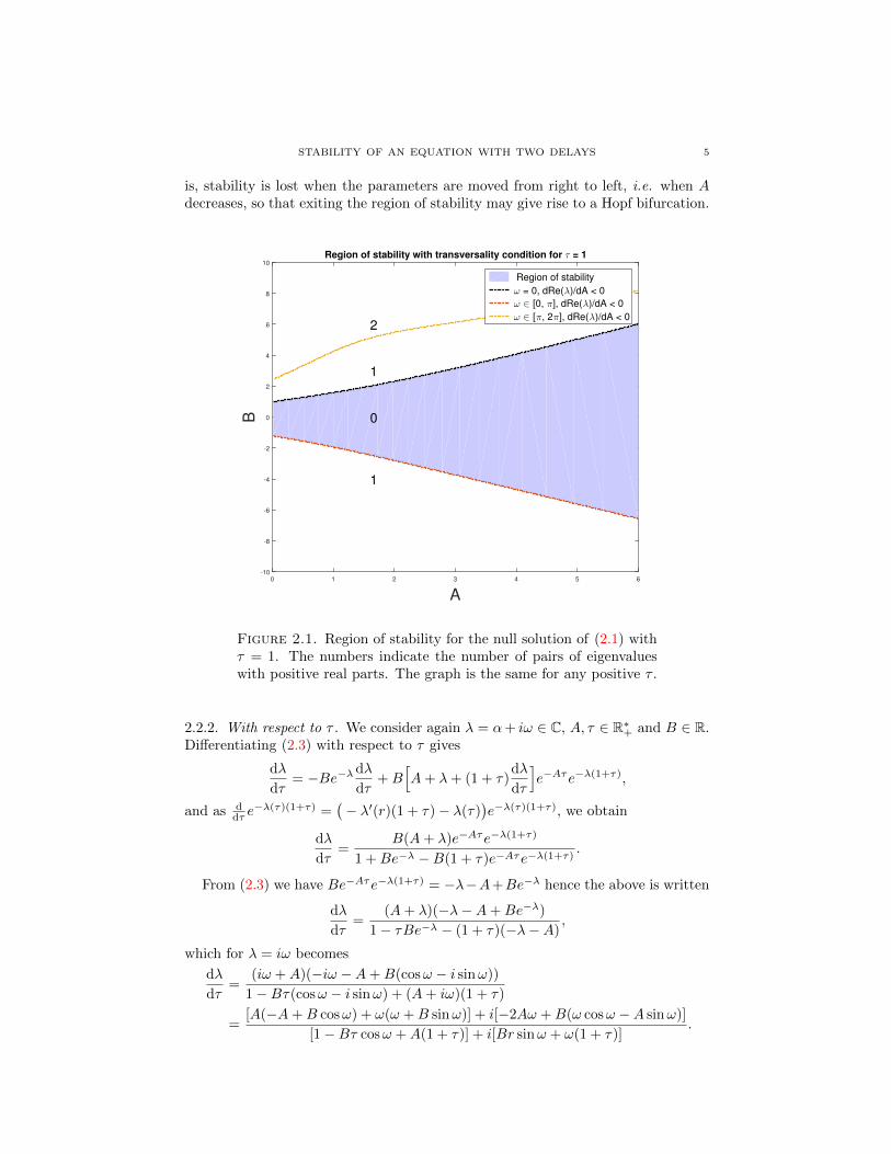
STABILITY OF AN EQUATION WITH TWO DELAYS 5
is, stability is lost when the parameters are moved from right to left, i.e. when Adecreases, so that exiting the region of stability may give rise to a Hopf bifurcation.
A0 1 2 3 4 5 6
B
-10
-8
-6
-4
-2
0
2
4
6
8
10
1
0
1
2
Region of stability with transversality condition for τ = 1
Region of stability
ω = 0, dRe(λ)/dA < 0
ω ∈ [0, π], dRe(λ)/dA < 0
ω ∈ [π, 2π], dRe(λ)/dA < 0
Figure 2.1. Region of stability for the null solution of (2.1) withτ = 1. The numbers indicate the number of pairs of eigenvalueswith positive real parts. The graph is the same for any positive τ .
2.2.2. With respect to τ . We consider again λ = α+ iω ∈ C, A, τ ∈ R∗+ and B ∈ R.Differentiating (2.3) with respect to τ gives
dλ
dτ= −Be−λ dλ
dτ+B
[A+ λ+ (1 + τ)
dλ
dτ
]e−Aτe−λ(1+τ),
and as ddτ e−λ(τ)(1+τ) =
(− λ′(r)(1 + τ)− λ(τ)
)e−λ(τ)(1+τ), we obtain
dλ
dτ=
B(A+ λ)e−Aτe−λ(1+τ)
1 +Be−λ −B(1 + τ)e−Aτe−λ(1+τ).
From (2.3) we have Be−Aτe−λ(1+τ) = −λ−A+Be−λ hence the above is written
dλ
dτ=
(A+ λ)(−λ−A+Be−λ)
1− τBe−λ − (1 + τ)(−λ−A),
which for λ = iω becomes
dλ
dτ=
(iω +A)(−iω −A+B(cosω − i sinω))
1−Bτ(cosω − i sinω) + (A+ iω)(1 + τ)
=[A(−A+B cosω) + ω(ω +B sinω)] + i[−2Aω +B(ω cosω −A sinω)]
[1−Bτ cosω +A(1 + τ)] + i[Br sinω + ω(1 + τ)].
6 L. BOULLU, L. PUJO-MENJOUET, J. BELAIR
Using the same decomposition as above, we get the sign of d Reλdτ as the sign of
Sτ (ω,A,B, τ) =ω2 −A(A+A2(1 + τ) + ω2(1 + τ) +B2τ)+(A+ (2τ + 1)A2 + ω2
)B cosω +
(1− 2Aτ
)ωB sinω.
We showed above that on the curve corresponding to ω = 0, that B = A1−e−Aτ >
0. A simple calculation implies that the sign of d Reλdτ is given by 1+A
1+A+Aτ − e−τA
which is always positive when both A and τ are strictly positive. This correspondsto a steady-state bifurcation.
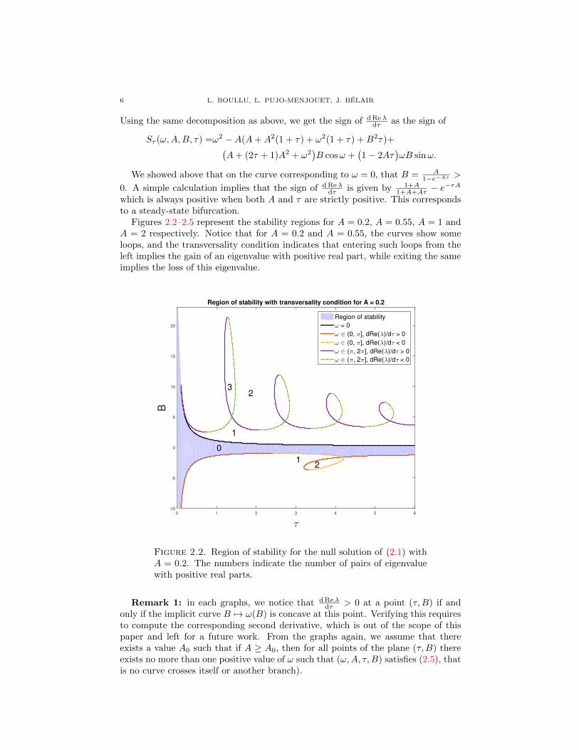
Figures 2.2–2.5 represent the stability regions for A = 0.2, A = 0.55, A = 1 andA = 2 respectively. Notice that for A = 0.2 and A = 0.55, the curves show someloops, and the transversality condition indicates that entering such loops from theleft implies the gain of an eigenvalue with positive real part, while exiting the sameimplies the loss of this eigenvalue.
τ
0 1 2 3 4 5 6
B
-10
-5
0
5
10
15
20
0
1
32
12
Region of stability with transversality condition for A = 0.2
Region of stability
ω = 0
ω ∈ (0, π], dRe(λ)/dτ > 0
ω ∈ (0, π], dRe(λ)/dτ < 0
ω ∈ (π, 2π], dRe(λ)/dτ > 0
ω ∈ (π, 2π], dRe(λ)/dτ < 0
Figure 2.2. Region of stability for the null solution of (2.1) withA = 0.2. The numbers indicate the number of pairs of eigenvaluewith positive real parts.
Remark 1: in each graphs, we notice that d Reλdτ > 0 at a point (τ,B) if and
only if the implicit curve B 7→ ω(B) is concave at this point. Verifying this requiresto compute the corresponding second derivative, which is out of the scope of thispaper and left for a future work. From the graphs again, we assume that thereexists a value A0 such that if A ≥ A0, then for all points of the plane (τ,B) thereexists no more than one positive value of ω such that (ω,A, τ,B) satisfies (2.5), thatis no curve crosses itself or another branch).
STABILITY OF AN EQUATION WITH TWO DELAYS 7
τ
0 0.5 1 1.5 2 2.5 3 3.5 4
B
-15
-10
-5
0
5
10
15
Region of stability with transversality condition for A = 0.55
Region of stability
ω = 0
ω ∈ (0, π], dRe(λ)/dτ > 0
ω ∈ (0, π], dRe(λ)/dτ < 0
ω ∈ (π, 2π], dRe(λ)/dτ > 0
ω ∈ (π, 2π], dRe(λ)/dτ < 0
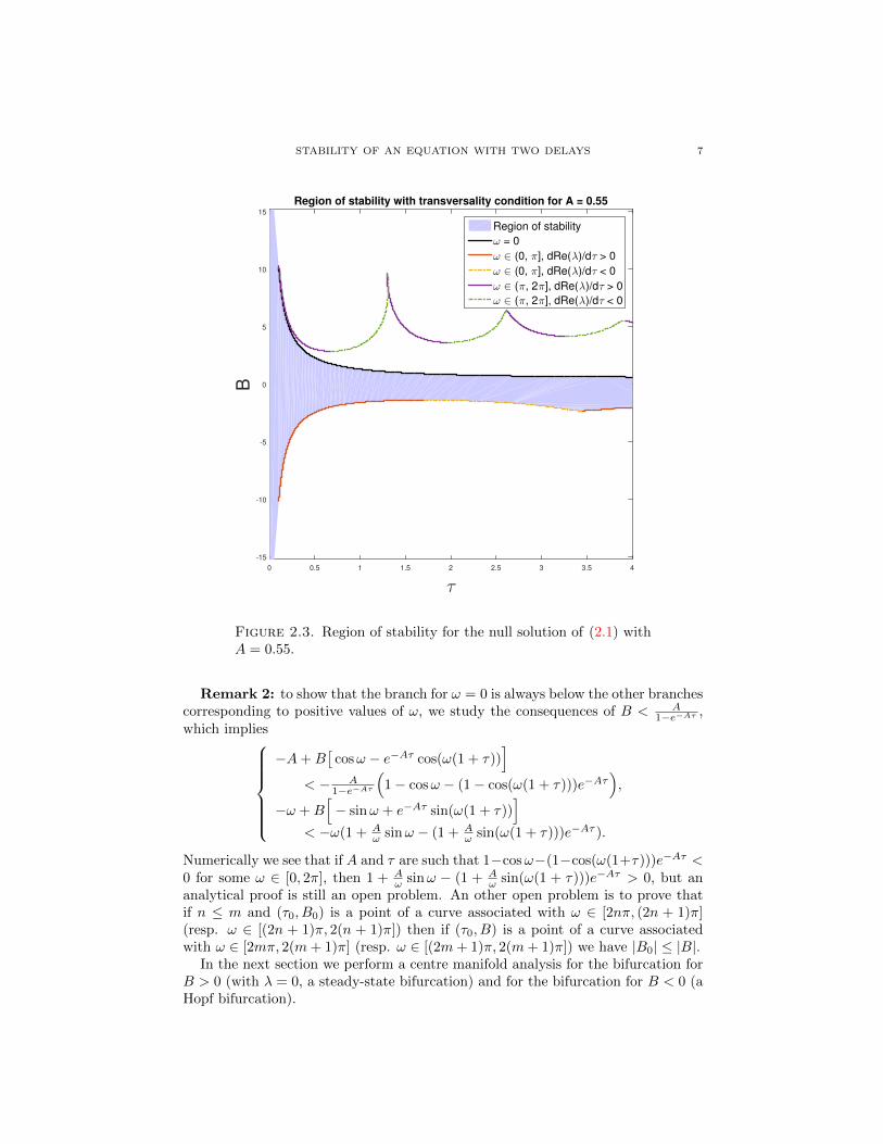
Figure 2.3. Region of stability for the null solution of (2.1) withA = 0.55.
Remark 2: to show that the branch for ω = 0 is always below the other branchescorresponding to positive values of ω, we study the consequences of B < A
1−e−Aτ ,which implies
−A+B[
cosω − e−Aτ cos(ω(1 + τ))]
< − A1−e−Aτ
(1− cosω − (1− cos(ω(1 + τ)))e−Aτ
),
−ω +B[− sinω + e−Aτ sin(ω(1 + τ))
]< −ω(1 + A
ω sinω − (1 + Aω sin(ω(1 + τ)))e−Aτ ).
Numerically we see that if A and τ are such that 1−cosω−(1−cos(ω(1+τ)))e−Aτ <0 for some ω ∈ [0, 2π], then 1 + A
ω sinω − (1 + Aω sin(ω(1 + τ)))e−Aτ > 0, but an
analytical proof is still an open problem. An other open problem is to prove thatif n ≤ m and (τ0, B0) is a point of a curve associated with ω ∈ [2nπ, (2n + 1)π](resp. ω ∈ [(2n + 1)π, 2(n + 1)π]) then if (τ0, B) is a point of a curve associatedwith ω ∈ [2mπ, 2(m+ 1)π] (resp. ω ∈ [(2m+ 1)π, 2(m+ 1)π]) we have |B0| ≤ |B|.
In the next section we perform a centre manifold analysis for the bifurcation forB > 0 (with λ = 0, a steady-state bifurcation) and for the bifurcation for B < 0 (aHopf bifurcation).

8 L. BOULLU, L. PUJO-MENJOUET, J. BELAIR
τ
0 0.5 1 1.5 2 2.5 3 3.5 4
B
-10
-5
0
5
10
Region of stability with transversality condition for A = 1
Region of stability
ω = 0
ω ∈ (0, π], dRe(λ)/dτ > 0
ω ∈ (0, π], dRe(λ)/dτ < 0
ω ∈ (π, 2π], dRe(λ)/dτ > 0
ω ∈ (π, 2π], dRe(λ)/dτ < 0
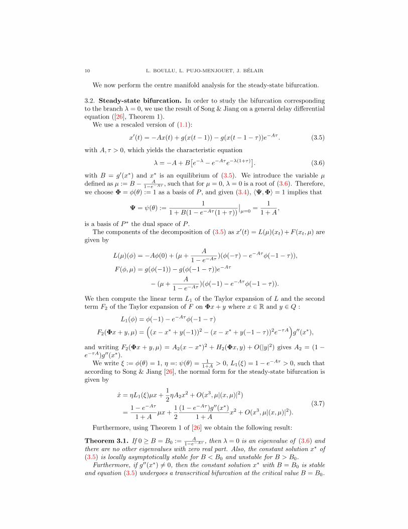
Figure 2.4. Region of stability for the null solution of (2.1) withA = 1.
3. Centre manifold analysis for simple bifurcations. When an eigenvaluewith positive real part appears through a steady-state bifurcation, the change ofstability is generically of one of two types. Either one new locally stable equilibriumpoint appears, in which case the bifurcation is called “transcritical”, or two newlocally stable equilibrium points appear, in which case the bifurcation is called“pitchfork bifurcation”. Similarly, when a pair of eigenvalues with positive realparts appears through a Hopf bifurcation, the change in stability is generically ofone of two types. If a stable limit cycle appears when the Hopf bifurcation occurs,it is said to be a “supercritical Hopf bifurcation”, and if an unstable limit cycledisappears when the Hopf bifurcation occurs, it is said to be a “subcritical Hopfbifurcation”. In both instances, to determine the type of the bifurcation we canperform a centre manifold analysis for the steady-state bifurcation and for simpleHopf bifurcation.
3.1. Theoretical basis for centre manifold analysis (from [8]). We considerthe general delay differential equation with two delays expressed as
x′(t) = L(x(t), x(t− τ1), x(t− τ2)) + f(x(t), x(t− τ1), x(t− τ2)), (3.1)
STABILITY OF AN EQUATION WITH TWO DELAYS 9
τ
0 0.5 1 1.5 2 2.5 3 3.5 4
B
-10
-5
0
5
10
Region of stability with transversality condition for A = 2
Region of stability
ω = 0
ω ∈ (0, π], dRe(λ)/dτ > 0
ω ∈ (0, π], dRe(λ)/dτ < 0
ω ∈ (π, 2π], dRe(λ)/dτ > 0
ω ∈ (π, 2π], dRe(λ)/dτ < 0
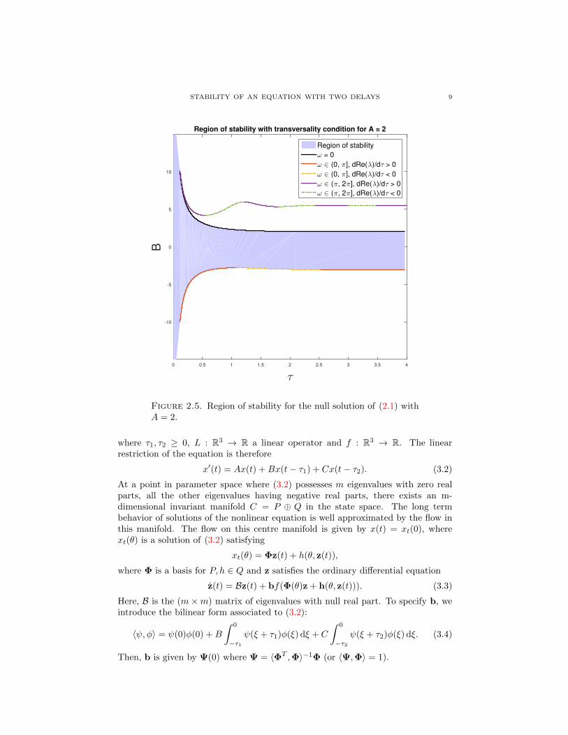
Figure 2.5. Region of stability for the null solution of (2.1) withA = 2.
where τ1, τ2 ≥ 0, L : R3 → R a linear operator and f : R3 → R. The linearrestriction of the equation is therefore
x′(t) = Ax(t) +Bx(t− τ1) + Cx(t− τ2). (3.2)
At a point in parameter space where (3.2) possesses m eigenvalues with zero realparts, all the other eigenvalues having negative real parts, there exists an m-dimensional invariant manifold C = P ⊕ Q in the state space. The long termbehavior of solutions of the nonlinear equation is well approximated by the flow inthis manifold. The flow on this centre manifold is given by x(t) = xt(0), wherext(θ) is a solution of (3.2) satisfying
xt(θ) = Φz(t) + h(θ, z(t)),
where Φ is a basis for P, h ∈ Q and z satisfies the ordinary differential equation
z(t) = Bz(t) + bf(Φ(θ)z + h(θ, z(t))). (3.3)
Here, B is the (m×m) matrix of eigenvalues with null real part. To specify b, weintroduce the bilinear form associated to (3.2):
〈ψ, φ〉 = ψ(0)φ(0) +B
∫ 0
−τ1ψ(ξ + τ1)φ(ξ) dξ + C
∫ 0
−τ2ψ(ξ + τ2)φ(ξ) dξ. (3.4)
Then, b is given by Ψ(0) where Ψ = 〈ΦT ,Φ〉−1Φ (or 〈Ψ,Φ〉 = 1).
10 L. BOULLU, L. PUJO-MENJOUET, J. BELAIR
We now perform the centre manifold analysis for the steady-state bifurcation.
3.2. Steady-state bifurcation. In order to study the bifurcation correspondingto the branch λ = 0, we use the result of Song & Jiang on a general delay differentialequation ([26], Theorem 1).
We use a rescaled version of (1.1):
x′(t) = −Ax(t) + g(x(t− 1))− g(x(t− 1− τ))e−Aτ . (3.5)
with A, τ > 0, which yields the characteristic equation
λ = −A+B[e−λ − e−Aτe−λ(1+τ)
]. (3.6)
with B = g′(x∗) and x∗ is an equilibrium of (3.5). We introduce the variable µdefined as µ := B − A
1−e−Aτ , such that for µ = 0, λ = 0 is a root of (3.6). Therefore,
we choose Φ = φ(θ) := 1 as a basis of P , and given (3.4), 〈Ψ,Φ〉 = 1 implies that
Ψ = ψ(θ) :=1
1 +B(1− e−Aτ (1 + τ))
∣∣µ=0
=1
1 +A,
is a basis of P ∗ the dual space of P .The components of the decomposition of (3.5) as x′(t) = L(µ)(xt) +F (xt, µ) are
given by
L(µ)(φ) = −Aφ(0) + (µ+A
1− e−Aτ)(φ(−τ)− e−Aτφ(−1− τ)),
F (φ, µ) = g(φ(−1))− g(φ(−1− τ))e−Aτ
− (µ+A
1− e−Aτ)(φ(−1)− e−Aτφ(−1− τ)).
We then compute the linear term L1 of the Taylor expansion of L and the secondterm F2 of the Taylor expansion of F on Φx+ y where x ∈ R and y ∈ Q :
L1(φ) = φ(−1)− e−Aτφ(−1− τ)
F2(Φx+ y, µ) =(
(x− x∗ + y(−1))2 − (x− x∗ + y(−1− τ))2e−τA)g′′(x∗),
and writing F2(Φx + y, µ) = A2(x − x∗)2 + H2(Φx, y) + O(|y|2) gives A2 = (1 −e−τA)g′′(x∗).
We write ξ := φ(θ) = 1, η =: ψ(θ) = 11+A > 0, L1(ξ) = 1− e−Aτ > 0, such that
according to Song & Jiang [26], the normal form for the steady-state bifurcation isgiven by
x = ηL1(ξ)µx+1
2ηA2x
2 +O(x3, µ|(x, µ)|2)
=1− e−Aτ
1 +Aµx+
1
2
(1− e−Aτ )g′′(x∗)
1 +Ax2 +O(x3, µ|(x, µ)|2).
(3.7)
Furthermore, using Theorem 1 of [26] we obtain the following result:
Theorem 3.1. If 0 ≥ B = B0 := A1−e−Aτ , then λ = 0 is an eigenvalue of (3.6) and
there are no other eigenvalues with zero real part. Also, the constant solution x∗ of(3.5) is locally asymptotically stable for B < B0 and unstable for B > B0.
Furthermore, if g′′(x∗) 6= 0, then the constant solution x∗ with B = B0 is stableand equation (3.5) undergoes a transcritical bifurcation at the critical value B = B0.

STABILITY OF AN EQUATION WITH TWO DELAYS 11
Remark: if g′′(x∗) = 0, the possibility of a pitchfork bifurcation can be evaluatedusing a normal form of higher order than the one in (3.7). However, this is out ofthe scope of this paper.
We now perform the centre manifold analysis for a single Hopf bifurcation.
3.3. Single Hopf. In the following, we employ the Taylor expansion of (1.1) withscaling about an equilibrium x∗, given by
y′(t) = −Ay(t) +B(y(t− 1)− e−Aτy(t− 1− τ)) +C
2(y2(t− 1)
− e−Aτy2(t− 1− τ)) +D
6(y3(t− 1)− e−Aτy3(t− 1− τ)) +O(y4
t )
= L(y(t), y(t− 1), y(t− 1− τ)) + f(y(t), y(t− 1), y(t− 1− τ)) +O(y4t ),
(3.8)with A = γτ1 > 0, B = g′(x∗)τ1, C = g′′(x∗)τ1, D = g′′′(x∗)τ1 and τ = τ2/τ1 > 0.
In order to obtain the type of the Hopf bifurcation, we use the method of Camp-bell [8] for compute the centre manifold using the symbolic algebra package Maple.We give an overview of the different steps of computation:
• we start by computing the vector b using (3.4) and the fact that for the singleHopf bifurcation we have Φ = (φ1, φ2) = (sin(ωθ), cos(ωθ)) ;
• we then introduce the function
h2(θ, z) = h11(θ)x2 + h12(θ)xy + h22(θ)y2,
and we compute the functions hij by solving the following partial differentialequation (see [8], eq. 8.31):
∂h2
∂θ(θ, z) +O(||z||3) =
∂h2
∂z(θ, z)Bz + Φ(θ)Ψ(0)F2(Φ(θ)u) +O(||z||3)
The arbitrary constants are determined using a second partial differentialequation given in [8] (eq. 8.32) ;
• the equation (3.3) becomes
x′ = −ωy + b1(f11x
2 + f12xy + f22y2 + f111x
3 + f112x2y + f122xy
2 + f222y3),
y′ = ωx+ b2(f11x
2 + f12xy + f22y2 + f111x
3 + f112x2y + f122xy
2 + f222y3),
and the type of the Hopf bifurcation is determined (see [14], eq. 3.4.11) bythe sign of
a =1
8(3b1f111 + b1f122 + b2f112 + 3b2f222)
+1
8ω((b21 − b22)f12(f11 + f22) + 2b1b2(f2
22 − f211)).
(3.9)
The Maple commands are available online1. The final expression of a involvesderivatives of g of order higher than two, such that it is not possible to computeits value without choosing a function g beforehand (see next section). Because thisimplies a constraint on B, the value a is computed on single points rather than onthe whole stability boundary as it can be seen in [1].
In the next section, we present a detailed analysis of the bifurcations occurringat parameter values where two pairs of purely imaginary eigenvalues exist.
1http://math.univ-lyon1.fr/~pujo/platelet-regulation.html

12 L. BOULLU, L. PUJO-MENJOUET, J. BELAIR
4. Centre manifold analysis for double Hopf bifurcation. In the double Hopfcase, the type of the bifurcation is indicated by four coefficients a11, a12, a21, a22
which are the equivalent of a in the simple Hopf case. However, there is no explicitexpression of these coefficients (an equivalent to (3.9)) in the literature. Thereforethey need to be computed using the symbolic algebra package Maple.
4.1. Computing a11, a12, a21, a22 using Maple. The computation ofa11, a12, a21, a22 from a system of the form
x = −ω1y + F 1111x
3 + F 1112x
2y + F 1114x
2u+ F 1114x
2v + . . . ,
y = ω1x+ F 2111x
3 + F 2112x
2y + F 2114x
2u+ F 2114x
2v + . . . ,
u = −ω2v + F 3111x
3 + F 3112x
2y + F 3114x
2u+ F 3114x
2v + . . . ,
v = ω2u+ F 4111x
3 + F 4112x
2y + F 4114x
2u+ F 4114x
2v + . . . ,
(4.1)
also written xyuv
=
0 −ω1 0 0ω1 0 0 00 0 0 −ω2
0 0 ω2 0
xyuv
+
f1(x, y, u, v)f2(x, y, u, v)f3(x, y, u, v)f4(x, y, u, v)
, (4.2)
of a double Hopf bifurcation follows the steps explained by Guckenheimer [14] inthe “appendix to Section 3.4”. It relies on writing (4.2) as a complex system, thatis
z1 = λ1z1 + h(z1, z1, z2, z2),
z2 = λ2z2 + g(z1, z1, z2, z2),(4.3)
with λi = iωi, z1 = x+ iy, z2 = u+ iv, and writing the normal form for the doubleHopf as a complex system, that is
w′1 = λ1w1 + c11w21w1 + c12w1w2w2 +O(|w1, w2|5) =: λ1w1 + h1(w1, w1, w2, w2),
w′2 = λ2w1 + c21w1w1w2 + c22w22w2 +O(|w1, w2|5) =: λ2w2 + h2(w1, w1, w2, w2).
(4.4)To transform (4.3) to (4.4), we use the near identity transformation
z1 = w1 + Ψ(w1, w1, w2, w2), Ψ = O(|w1, w2|2),
z2 = w2 + Φ(w1, w1, w2, w2), Φ = O(|w1, w2|2).(4.5)
Substituting (4.5) in (4.3) and using (4.4), we obtain twopartial differential equations PDE1 and PDE2 (see the fileBP-MB 2018 - computations double Hopf.mw online2).
We give an overview of the different steps of computation performed in Maple :
• We introduce the Taylor expansion to the second order of Φ,Ψ, h, g, that wesubstitute in PDE1 and PDE2. Equating coefficients of wi, wj , wiwj andwiwj we obtain expressions of the partial derivatives of Φ,Ψ as functions ofpartial derivatives of h, g.
• We introduce the Taylor expansion to the third order of h, g that we substitutein PDE1 and PDE2. Equating coefficients of w2
1w1, w1w2w2, w1w1w2 andw2
2w2, we obtain expressions of the coefficients c11, c12, c21, c22 as functions ofthe partial derivatives of h, g. The coefficients of interest a11, a12, a21, a22 aregiven as aij = Re(cij).
2http://math.univ-lyon1.fr/~pujo/platelet-regulation.html
STABILITY OF AN EQUATION WITH TWO DELAYS 13
• To obtain expressions of the partial derivatives of h, g as functions of thepartial derivatives of fi, i = 1, 2, 3, 4, we use the Taylor expansion to the thirdorder of fi, i = 1, 2, 3, 4 and the fact that h = f1 + if2, g = f3 + if4.
• The partial derivatives of fi, i = 1, 2, 3, 4 are computed as functions of theF lijk, i, j, k, l = 1, 2, 3, 4 of (4.1).
From there, the computation of the F lijk, i, j, k, l = 1, 2, 3, 4 of (4.1) is performed
following the adaptation of the method of Campbell [8] used in Section 3.3 to thecase of double Hopf bifurcation. The Maple commands are available oneline3.
4.2. Calculating the centre manifold of the double Hopf bifurcation. Inthe case of the double Hopf bifurcation, there are two values of ω satisfying (2.5)for the same values of A,B and τ :
A = +B[
cosω1 − e−Aτ cos(ω1(1 + τ))],
ω1 = B[− sinω1 + e−Aτ sin(ω1(1 + τ))
],
0 = A+B[
cosω2 − e−Aτ cos(ω2(1 + τ))],
ω2 = B[− sinω2 + e−Aτ sin(ω2(1 + τ))
].
And the elements needed to write (3.3) are
Φ = (φ1, φ2, φ3, φ4) = (sin(ω1θ), cos(ω1θ), sin(ω2θ), cos(ω2θ)), z = (x, y, u, v)T ,(4.6)
such that Φz = sin(ω1θ)x+ cos(ω1θ)y + sin(ω2θ)u+ cos(ω2θ)v,
B =
0 −ω1 0 0ω1 0 0 00 0 0 −ω2
0 0 ω2 0
, and b =
K12,K22,K34,K44
,
with K =
〈ΦT
12,Φ12〉T
D212
0
0〈ΦT
34,Φ34〉T
D234
, D2ij = det〈ΦT
12,Φ12〉 and Φij = (φi, φj).
In order to obtain the type of the Hopf bifurcation, we use the method of Camp-bell [8] for calculating centre manifold using the symbolic algebra package Maple.The algorithm using Maple and its results are available online4. For sake of clarity,we decide to only give an overview of the different steps of computation to them:
• we start by computing the vector b using (3.4);• we then introduce the function
h2(θ, z) = h11(θ)x2 + h12(θ)xy + h13(θ)xu+ h14(θ)xv + h22(θ)y2
+ h23(θ)yu+ h24(θ)yv + h33(θ)u2 + h34(θ)uv + h44(θ)v2
and we compute the functions hii by solving the following partial differentialequation (see [8], equation 8.31):
∂h2
∂θ+O(||z||3) =
∂h2
∂z(θ, z)Bz + Φ(θ)Ψ(0)F2(Φ(θ)u) +O(||z||3)
The arbitrary constants are determined using a second partial differentialequation (see [8], equation 8.32);
3http://math.univ-lyon1.fr/~pujo/platelet-regulation.html4http://math.univ-lyon1.fr/~pujo/platelet-regulation.html
14 L. BOULLU, L. PUJO-MENJOUET, J. BELAIR
• we then obtain the equation (3.3) under the form (4.1).
Combining with the expressions of a11, a12, a21, a22 as functions of the coefficientsof (4.1), we have an expression of a11, a12, a21, a22 as a function of A,B,C,D, ω andτ . The Maple commands are available online5.
4.3. From the values of a11, a12, a21, a22 to the descriptions of the flowsnear the double Hopf. We introduce the continuous functions µ1, µ2,Ω1,Ω2 onR2
+ describing the branches of eigenvalues associated with the purely imaginaryeigenvalues ω1 and ω2, i.e. such that for a point (τ,B),
λ1±(τ,B) = µ1(τ,B)± iΩ1(τ,B), and λ2±(τ,B) = µ2(τ,B)± iΩ2(τ,B)
are two pairs of simple complex-conjugate eigenvalues such that λ1+(τ0, B0) = iω1
and λ2+(τ0, B0) = iω2. According to the theory of centre manifold analysis, if(τ1, B1) is a point close to (τ0, B0), then System (4.1) is approximated by a systemin radial components given by
r1 = µ1(τ1, B1)r1 + a11r31 + a12r1r
22,
r2 = µ2(τ1, B1)r2 + a21r21r2 + a22r
32,
θ1 = ω1(τ1, B1),
θ2 = ω2(τ1, B1),
(4.7)
and the possible dynamics are explored by studying the “amplitude system” forr1, r2 ≥ 0 given by
r1 = µ1(τ1, B1)r1 + a11r31 + a12r1r
22,
r2 = µ2(τ1, B1)r2 + a21r21r2 + a22r
32.
(4.8)
Indeed, equivalences have been established [17] between the positions of the equi-libria of (4.8) and the dynamics of the solutions of (4.7):
• an equilibrium at r1 = r2 = 0 for (4.8) corresponds to an equilibrium point atthe origin for (4.7) ;
• an non-trivial equilibrium on one of the axis for (4.8) corresponds to cycle for(4.7) ;
• an equilibrium with r1, r2 > 0 for (4.8) corresponds to two-dimensional torusfor (4.7) ;
• a limit cycle for (4.8) corresponds to three-dimensional torus for (4.7).
We find in Kuznetsov ([17], Section 8.6.2) a description of all the possible subcases
(called the “unfolding” of (4.8)), depending on the signs of a11a22, θ :=a12
a22, δ :=
a21
a11and θδ − 1.
4.4. Application to the equation x′(t) = −γx(t) + g(x(t − τ1)) + g(x(t − τ1 −τ2))e−γτ2 . We go back to the bifurcation regions of, and focus on the double Hopfbifurcation happening when the stability boundary of B < 0 crosses itself. As saidbefore, a change in stability occurs through a Hopf bifurcation only if B < 0, andwe see that there exist ω1, ω2 such that (τ(ω1), B(ω1)) = (τ(ω2), B(ω2)) = (τ0, B0)with B0 = −1.6006 < 0 and τ0 = 4.1693 (see Figure 2.2).
Because the expressions of aij involve C and D, we need to fix g such thatthe point (τ,B) corresponds to the crossing of the lower stability boundary seen
5http://math.univ-lyon1.fr/~pujo/platelet-regulation.html
STABILITY OF AN EQUATION WITH TWO DELAYS 15
on Figure 2.2 : we choose g(x) := f0σn
σn+xn + β0 with f0 = 5 × 10¹⁰, β0 = 0.01,
σ = 8 × 10⁹ and n = 10.166. In this case, and assuming that the curve decreaseswith τ corresponds to ω1, we have
a11 > 0, a12 > 0, a21 < 0, a22 < 0,
θ :=a12
a22< 0, δ :=
a21
a11< 0, θδ − 1 > 0,
(4.9)
which corresponds to subcase VI of the “complex” case in Kuznetsov numberingscheme (see [17] p. 363). The Maple commands are available online6.
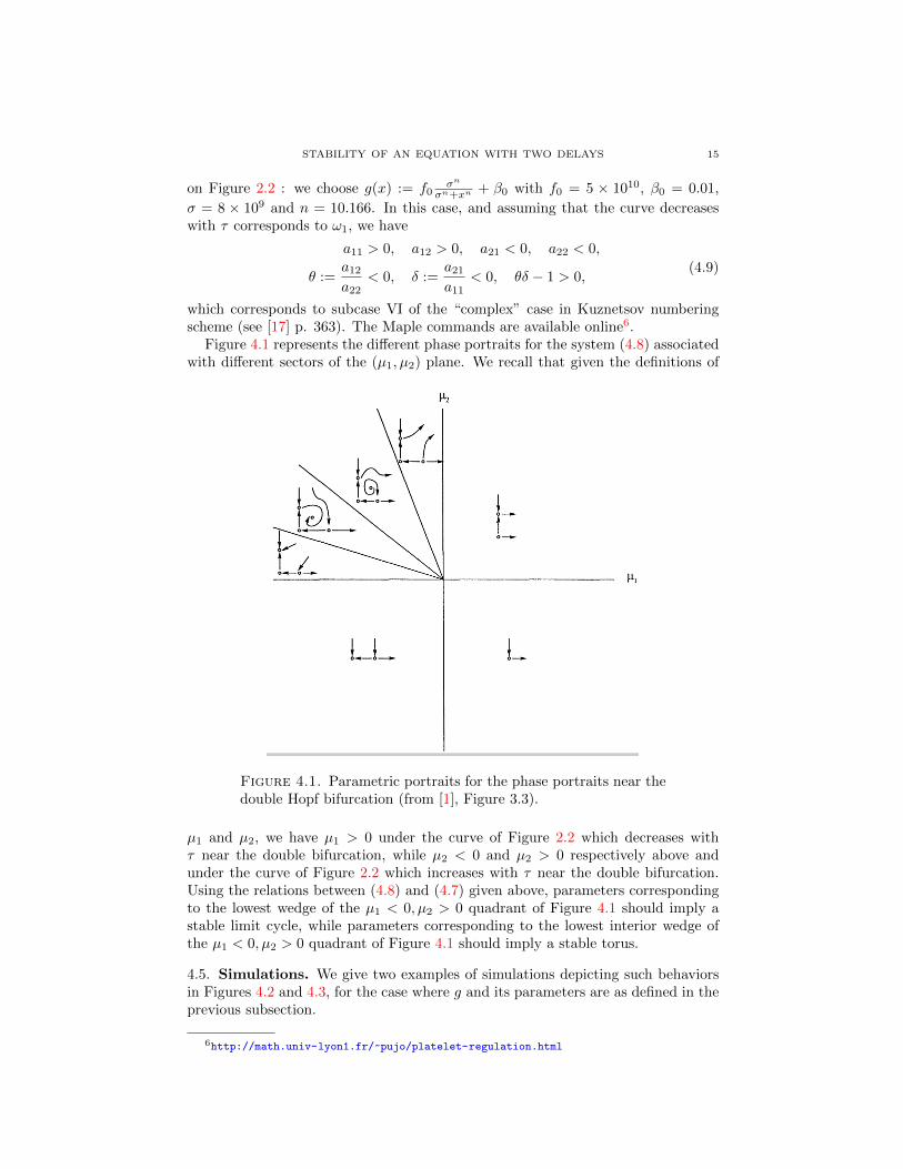
Figure 4.1 represents the different phase portraits for the system (4.8) associatedwith different sectors of the (µ1, µ2) plane. We recall that given the definitions of
Figure 4.1. Parametric portraits for the phase portraits near thedouble Hopf bifurcation (from [1], Figure 3.3).
µ1 and µ2, we have µ1 > 0 under the curve of Figure 2.2 which decreases withτ near the double bifurcation, while µ2 < 0 and µ2 > 0 respectively above andunder the curve of Figure 2.2 which increases with τ near the double bifurcation.Using the relations between (4.8) and (4.7) given above, parameters correspondingto the lowest wedge of the µ1 < 0, µ2 > 0 quadrant of Figure 4.1 should imply astable limit cycle, while parameters corresponding to the lowest interior wedge ofthe µ1 < 0, µ2 > 0 quadrant of Figure 4.1 should imply a stable torus.
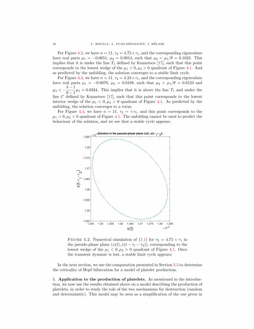
4.5. Simulations. We give two examples of simulations depicting such behaviorsin Figures 4.2 and 4.3, for the case where g and its parameters are as defined in theprevious subsection.
6http://math.univ-lyon1.fr/~pujo/platelet-regulation.html
16 L. BOULLU, L. PUJO-MENJOUET, J. BELAIR
For Figure 4.2, we have n = 11, τ2 = 4.75×τ1, and the corresponding eigenvalueshave real parts µ1 = −0.0651, µ2 = 0.0014, such that µ2 < µ1/θ = 0.1023. Thisimplies that it is under the line T1 defined by Kuznetsov [17], such that this pointcorresponds to the lowest wedge of the µ1 < 0, µ2 > 0 quadrant of Figure 4.1. Andas predicted by the unfolding, the solution converges to a stable limit cycle.
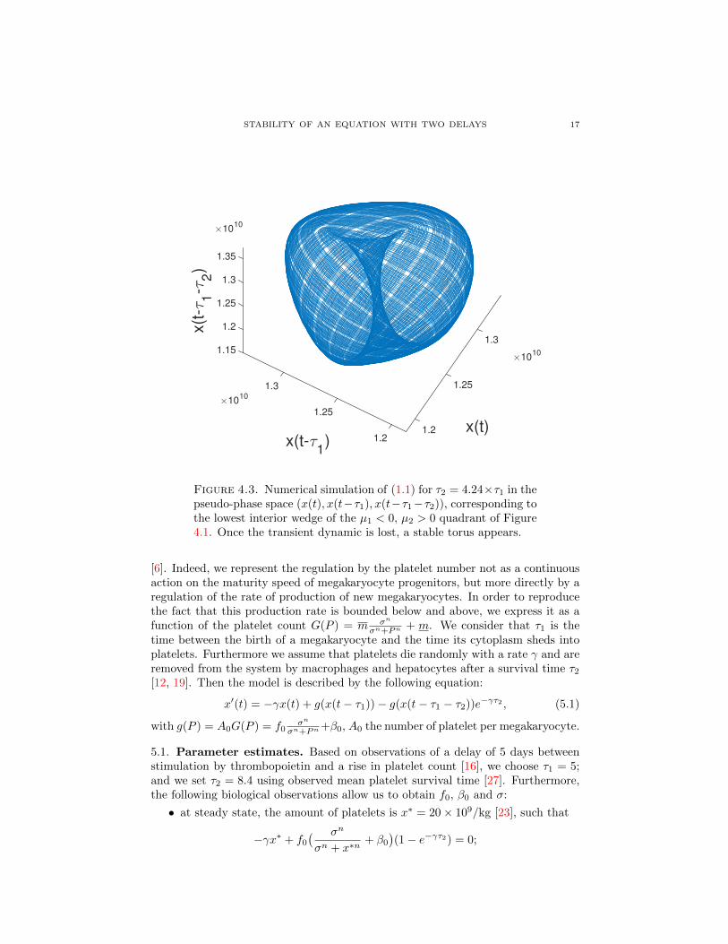
For Figure 4.3, we have n = 11, τ2 = 4.24×τ1, and the corresponding eigenvalueshave real parts µ1 = −0.0078, µ2 = 0.0188, such that µ2 > µ1/θ = 0.0123 and
µ2 < −δ − 1
θ − 1µ1 = 0.0334. This implies that it is above the line T1 and under the
line C defined by Kuznetsov [17], such that this point corresponds to the lowestinterior wedge of the µ1 < 0, µ2 > 0 quadrant of Figure 4.1. As predicted by theunfolding, the solution converges to a torus.
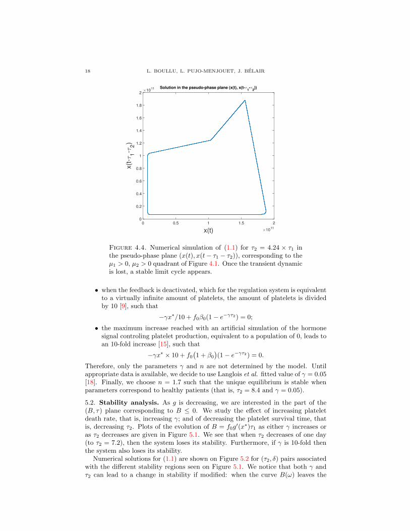
For Figure 4.4, we have n = 11, τ2 = ×τ1, and this point corresponds to theµ1 > 0, µ2 > 0 quadrant of Figure 4.1. The unfolding cannot be used to predict thebehaviour of the solution, and we see that a stable cycle appears.
x(t) ×1010
1.245 1.25 1.255 1.26 1.265 1.27 1.275 1.28 1.285
x(t
-τ1-τ
2)
×1010
1.245
1.25
1.255
1.26
1.265
1.27
1.275
1.28
1.285
Solution in the pseudo-phase plane (x(t), x(t-τ1-τ
2))
Figure 4.2. Numerical simulation of (1.1) for τ2 = 4.75 × τ1 inthe pseudo-phase plane (x(t), x(t− τ1 − τ2)), corresponding to thelowest wedge of the µ1 < 0, µ2 > 0 quadrant of Figure 4.1. Oncethe transient dynamic is lost, a stable limit cycle appears.
In the next section, we use the computation presented in Section 3.3 to determinethe criticality of Hopf bifurcation for a model of platelet production.
5. Application to the production of platelets. As mentioned in the introduc-tion, we now use the results obtained above on a model describing the production ofplatelets, in order to study the role of the two mechanisms for destruction (randomand deterministic). This model may be seen as a simplification of the one given in
STABILITY OF AN EQUATION WITH TWO DELAYS 17
×1010
1.3
Solution in the pseudo-phase plane (y(t-τ1-τ
2),y(t))
x(t)
1.25
1.21.2
1.25
x(t-τ1)
1.3
×1010
×1010
1.35
1.15
1.2
1.25
1.3
x(t
-τ1-τ
2)
Figure 4.3. Numerical simulation of (1.1) for τ2 = 4.24×τ1 in thepseudo-phase space (x(t), x(t−τ1), x(t−τ1−τ2)), corresponding tothe lowest interior wedge of the µ1 < 0, µ2 > 0 quadrant of Figure4.1. Once the transient dynamic is lost, a stable torus appears.
[6]. Indeed, we represent the regulation by the platelet number not as a continuousaction on the maturity speed of megakaryocyte progenitors, but more directly by aregulation of the rate of production of new megakaryocytes. In order to reproducethe fact that this production rate is bounded below and above, we express it as afunction of the platelet count G(P ) = m σn
σn+Pn + m. We consider that τ1 is thetime between the birth of a megakaryocyte and the time its cytoplasm sheds intoplatelets. Furthermore we assume that platelets die randomly with a rate γ and areremoved from the system by macrophages and hepatocytes after a survival time τ2[12, 19]. Then the model is described by the following equation:
x′(t) = −γx(t) + g(x(t− τ1))− g(x(t− τ1 − τ2))e−γτ2 , (5.1)
with g(P ) = A0G(P ) = f0σn
σn+Pn+β0, A0 the number of platelet per megakaryocyte.
5.1. Parameter estimates. Based on observations of a delay of 5 days betweenstimulation by thrombopoietin and a rise in platelet count [16], we choose τ1 = 5;and we set τ2 = 8.4 using observed mean platelet survival time [27]. Furthermore,the following biological observations allow us to obtain f0, β0 and σ:
• at steady state, the amount of platelets is x∗ = 20× 109/kg [23], such that
−γx∗ + f0
( σn
σn + x∗n+ β0
)(1− e−γτ2) = 0;
18 L. BOULLU, L. PUJO-MENJOUET, J. BELAIR
x(t) ×1011
0 0.5 1 1.5 2
x(t
-τ1-τ
2)
×1011
0
0.2
0.4
0.6
0.8
1
1.2
1.4
1.6
1.8
2
Solution in the pseudo-phase plane (x(t), x(t-τ1-τ
2))
Figure 4.4. Numerical simulation of (1.1) for τ2 = 4.24 × τ1 inthe pseudo-phase plane (x(t), x(t− τ1 − τ2)), corresponding to theµ1 > 0, µ2 > 0 quadrant of Figure 4.1. Once the transient dynamicis lost, a stable limit cycle appears.
• when the feedback is deactivated, which for the regulation system is equivalentto a virtually infinite amount of platelets, the amount of platelets is dividedby 10 [9], such that
−γx∗/10 + f0β0(1− e−γτ2) = 0;
• the maximum increase reached with an artificial simulation of the hormonesignal controling platelet production, equivalent to a population of 0, leads toan 10-fold increase [15], such that
−γx∗ × 10 + f0
(1 + β0
)(1− e−γτ2) = 0.
Therefore, only the parameters γ and n are not determined by the model. Untilappropriate data is available, we decide to use Langlois et al. fitted value of γ = 0.05[18]. Finally, we choose n = 1.7 such that the unique equilibrium is stable whenparameters correspond to healthy patients (that is, τ2 = 8.4 and γ = 0.05).
5.2. Stability analysis. As g is decreasing, we are interested in the part of the(B, τ) plane corresponding to B ≤ 0. We study the effect of increasing plateletdeath rate, that is, increasing γ; and of decreasing the platelet survival time, thatis, decreasing τ2. Plots of the evolution of B = f0g
′(x∗)τ1 as either γ increases oras τ2 decreases are given in Figure 5.1. We see that when τ2 decreases of one day(to τ2 = 7.2), then the system loses its stability. Furthermore, if γ is 10-fold thenthe system also loses its stability.
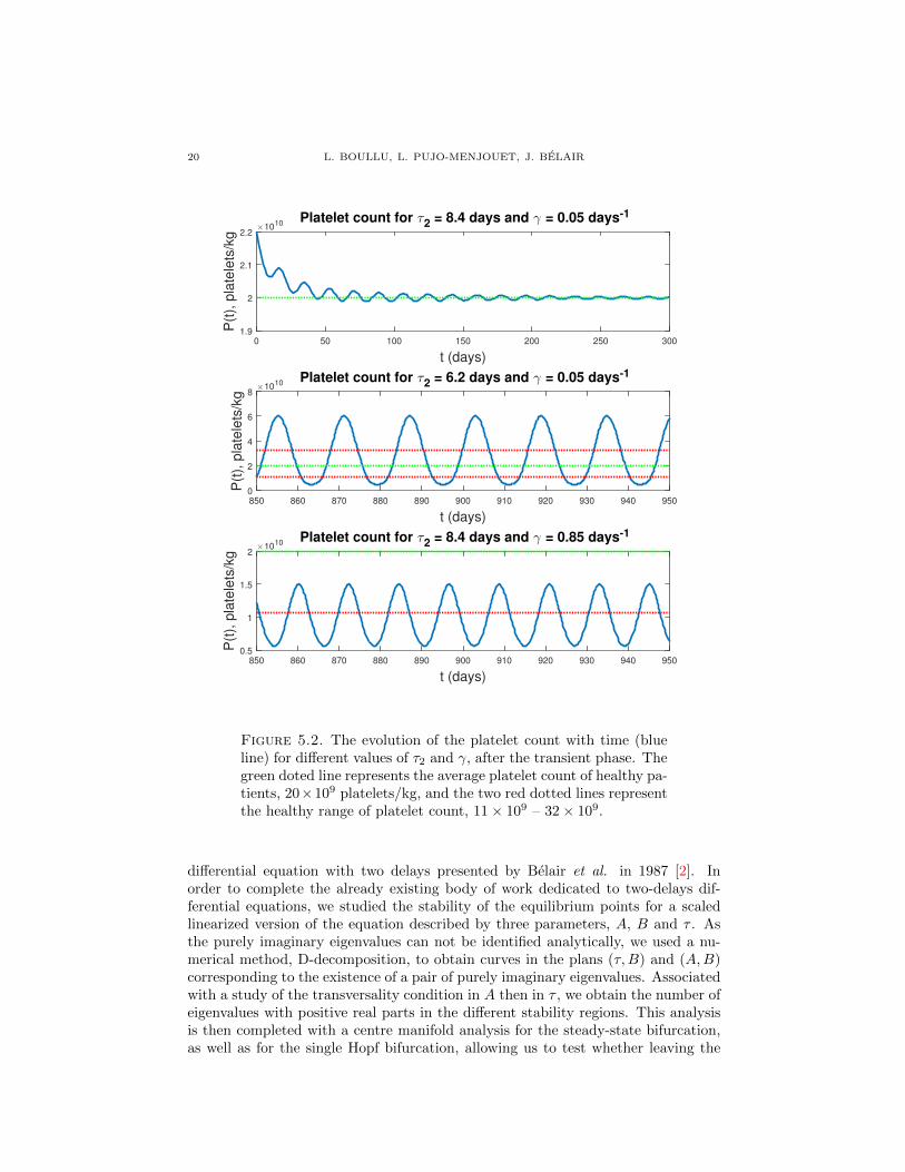
Numerical solutions for (1.1) are shown on Figure 5.2 for (τ2, δ) pairs associatedwith the different stability regions seen on Figure 5.1. We notice that both γ andτ2 can lead to a change in stability if modified: when the curve B(ω) leaves the

STABILITY OF AN EQUATION WITH TWO DELAYS 19
τ2
4 5 6 7 8 9 10
B
-2.5
-2
-1.5
-1
-0.5
0
Evolution of B as when τ2 decreases from 8.4
Region of stability
B(τ2)
τ2 = 8.4 (normal value)
Hopf Bifurcation
γ
0 0.1 0.2 0.3 0.4 0.5 0.6 0.7
B
-5
-4
-3
-2
-1
0Evolution of B as when γ increases from 0.05
Region of stability
B(γ)
γ = 0.05 (normal value)
Hopf Bifurcation
Figure 5.1. Stability as τ2 or γ are varied and other parametersare fixed. Blue dotted lines represent the values in healthy patients,and red dotted lines mark the limits after which the equilibrium isunstable. We see that when τ2 decreases of one day (to τ2 = 7.2),then the system loses its stability. Furthermore, if γ is multipliedmore than 12 times (to γ = 0.625) then the system also loses itsstability.
zone of stability, a Hopf bifurcation occurs. Furthermore, the criticality of the Hopfbifurcation is computed in both cases using the expression (3.9) of a computedin Maple (see online7). In both cases, a is negative such that the bifurcation issupercritical and a locally stable periodic solution appears, as seen on the solutionsobtained numerically.
Other characteristics of the dynamics change differently depending on the bifur-cation parameter: the main consequence of decreasing τ2 is an increase in amplitude,but increasing γ decreases the overall value of platelet count. However, from a clin-ical point of view a decrease in platelet survival time τ2 seems to induce a morethreatening chronic thrombocytopenia than a change in γ, as well as inducing achronic thrombocytosis.
6. Conclusion. In an attempt to model the quantity of platelets in the bloodas affected by both a random and an age-related destruction, we analyze a delay
7http://math.univ-lyon1.fr/~pujo/platelet-regulation.html
20 L. BOULLU, L. PUJO-MENJOUET, J. BELAIR
t (days)
0 50 100 150 200 250 300
P(t
), p
late
lets
/kg
×1010
1.9
2
2.1
2.2
Platelet count for τ2 = 8.4 days and γ = 0.05 days-1
t (days)
850 860 870 880 890 900 910 920 930 940 950
P(t
), p
late
lets
/kg
×1010
0
2
4
6
8
Platelet count for τ2 = 6.2 days and γ = 0.05 days-1
t (days)
850 860 870 880 890 900 910 920 930 940 950
P(t
), p
late
lets
/kg
×1010
0.5
1
1.5
2
Platelet count for τ2 = 8.4 days and γ = 0.85 days-1
Figure 5.2. The evolution of the platelet count with time (blueline) for different values of τ2 and γ, after the transient phase. Thegreen doted line represents the average platelet count of healthy pa-tients, 20×109 platelets/kg, and the two red dotted lines representthe healthy range of platelet count, 11× 109 – 32× 109.
differential equation with two delays presented by Belair et al. in 1987 [2]. Inorder to complete the already existing body of work dedicated to two-delays dif-ferential equations, we studied the stability of the equilibrium points for a scaledlinearized version of the equation described by three parameters, A, B and τ . Asthe purely imaginary eigenvalues can not be identified analytically, we used a nu-merical method, D-decomposition, to obtain curves in the plans (τ,B) and (A,B)corresponding to the existence of a pair of purely imaginary eigenvalues. Associatedwith a study of the transversality condition in A then in τ , we obtain the number ofeigenvalues with positive real parts in the different stability regions. This analysisis then completed with a centre manifold analysis for the steady-state bifurcation,as well as for the single Hopf bifurcation, allowing us to test whether leaving the
STABILITY OF AN EQUATION WITH TWO DELAYS 21
region of stability through a Hopf bifurcation is associated with the onset of periodicsolutions. Furthermore, the existence of self-intersection in the stability boundaryassociated with Hopf bifurcation revealed the possibility of a double Hopf bifurca-tion, a phenomenon known to generate a variety of complex dynamical behaviors.Therefore we performed a centre manifold analysis near the point where a doublebifurcation occurs, revealing the possibility of torus-like dynamics near the regionwhere two eigenvalues with positive real parts exist.
Finally, coming back to the model for platelet production, we use the results onthe single Hopf bifurcation to explore the impact of an increase in death rate or adecrease in survival time on the onset of periodic dynamics, as we expected fromthe platelet-specific antibodies observed in patients with cyclic thrombocytopenia.We choose a megakaryocyte production rate which decreases when the plateletcount increases, while always staying strictly positive and finite. The parametersof this feedback function are identified using the normal mean platelet count as anequilibrium. Finally, we show that although stability is gained by going from leftto right in the plane (B, γ), taking in account the role of γ in the computation ofB = g′(x∗)τ1 enables to lose stability when increasing the death rate γ of platelets.The same counter-intuitive conclusion is obtained for a decrease of the survivaltime of platelets τ2. The extent of the change in τ2 necessary to induce oscillationsseems more reasonable than that of γ. In the cases of cyclic thrombocytopenia ofthe auto-immune type, platelet-specific antibodies are observed in patients blood.Therefore, our work indicates that auto-immune cyclic thrombocytopenia is morelikely to be due to a over-reactive system of old platelet removal, rather than toan increase random destruction of platelets of any age. However, this relies on thelikelihood of a small decrease of τ2 being more important than the likelihood of aimportant increase of γ, which needs to be confirmed with clinicians.
Notice that although regularities appear in the graphs of the stability curve, suchas an ordering in the curves corresponding to different intervals [π + 2nπ, 2(n +1)π], n ∈ N or a equivalence between the transversality condition and the concavityof the function B 7→ B(ω), we were not able to obtain an analytical proof for suchresults. Besides, we encountered difficulties in simulating the solutions of (1.1)corresponding the sections 1, 2 and 6 of the unfolding (Figure 4.1). These questionsare still open and will be the object of a future work.
Most works on the stability of two-delays differential equations focus on a limitedversion of (1.3). For example, Belair & Campbell [1] studied the case where A = 0and B = 1, and focused on the features of the stable regions in the plane (A, r2) asr1 increases. In particular, authors obtained intersecting stability curves associatedwith a double Hopf bifurcation. Using centre manifold analysis, they identifiedtwo sets of parameters such that near the double Hopf bifurcation, the unfoldingcorresponds to type Ib of Guckenheimer & Holmes [14] for one, and VIa for theother (which corresponds to the subcase VI of the “complex” case in Kuznetsovnumbering scheme (see [17] p. 363)). The authors were also able to show that whenr1 increases, the stability region becomes composed of disconnected stable regions,a feature previously thought to be impossible. Interestingly, while the choice offixing A to 0 simplifies the computation of the stability regions, the identificationof bifurcation type still relies on numerical methods. Using a normalization suchthat r1 = 1, Mahaffy et al. [21] focused on the stability regions in the 3D-space(A,B,C). Indeed, once A and r2 are fixed, the computation of the values of Band C corresponding to the existence of a pair of purely imaginary eigenvalues
22 L. BOULLU, L. PUJO-MENJOUET, J. BELAIR
is straightforward. In particular, the authors identified regions in the plane (R,A)corresponding to different configurations of the stability regions in the plane (B,C),and noticed that there exists two disconnected regions for A < 0. Mahaffy & Busken[7] returned later to the study of the stability regions in the plane (B,C) while thistime focusing on the differences observed between the case r2 ∈ Q and r2 /∈ Q.Finally, Besse [4] analyzed the stability of (1.3) by presenting the stability regionsfor C < 0, r1 and r2 fixed. The author introduced a change of variable x = A+Band y = −A+B, such that the stability for x < −C or for y < C is straightforward.The stability for y ≥ C, x ≥ −C, however, is non-trivial, as for high r2 it involvesintertwined loops. The author were nevertheless able to obtain a region of the plane(x, y) in which the system is stable for any r2 ≥ 0, at the condition C ≥ −π/r1. Inour case, a change of stability occurs once along an increase of a parameter of themodel. However, it is known that such a change in stability is sometimes reversedby increasing the parameter further. This is often the case when the coefficientsof the characteristic equation involve the delay, as in [24, 25]. In our case, thecoefficients do not involve the delays, and for the application that we study, wedo not have stability switches. However, it is not impossible that given differentparameters or functions our model would present stability switches as the use oftwo delays implies an increase in complexity such that delay-dependent coefficientsare not needed for stability switches. For example, disconnected stability regionshave been observed for such models by Belair and Campbell [1], which is a featureconducive to stability switches.
Although most of the aforementioned papers rely on the method of D-decomposition, they do not use it to study the effect of parameters changes aswe did in Section 5. Therefore we mention two papers dedicated to models of ery-thropoiesis (the production of red blood cells) applying it. In the first one, Belairet al. [3] studies the stability of the equilibrium of a system of two differentialequations with two delays, and the analysis relies on a characteristic equation givenby
(λ+ γ)(λ+ k) = −A(e−λT1 − e−γT1e−λ(T1+T2)),
where A depends on the steady state. It is a more complicated version of (1.3)with an additional λ2. Authors identify numerically the stability region in theplane (γ,A), and similarly to the conclusion presented in Section 5, stability isgained when one moves from left to right in the plane (A, γ) but the role of γ inthe computation of A implies that increasing γ can lead to instability. A similarphenomenon was obtained later by Mahaffy et al. [20] in a second paper on a modelof erythropoiesis with a state-dependent delay.
Finally, we notice that equation (1.1) can also be obtained by adding a survivaltime for platelets to a model of megakaryopoiesis whose stability was recently ana-lyzed [5]. In the case of this model, we have τ1 > τ2, which according to preliminarynumerical explorations (not shown) seems to imply that stability is not affected ofthe value of γ.
REFERENCES
[1] J. Belair and S. A. Campbell, Stability and Bifurcations of Equilibria in a Multiple-DelayedDifferential Equation, SIAM Journal on Applied Mathematics, 54 (1994), 1402–1424.
[2] J. Belair and M. C. Mackey, A Model for the Regulation of Mammalian Platelet Production,Annals of the New York Academy of Sciences, 504 (1987), 280–282.
[3] J. Belair, M. C. Mackey and J. M. Mahaffy, Age-structured and two delay models for ery-thropoiesis, Math. Biosciences, 128 (1995), 317–346.
STABILITY OF AN EQUATION WITH TWO DELAYS 23
[4] A. Besse, Modelisation Mathematique de La Leucemie Myelode Chronique, Ph.D thesis, Uni-versite Claude Bernard Lyon 1, 2017.
[5] L. Boullu, M. Adimy, F. Crauste and L. Pujo-Menjouet, Oscillations and Asymptotic Con-
vergence for a Delay Differential Equation Modeling Platelet Production, Discrete and Con-tinuous Dynamical Systems Series B , 24 (2019), 2417–2442.
[6] L. Boullu, L. Pujo-Menjouet and J. Wu, A model for megakaryopoiesis with state-dependentdelay, submitted.
[7] T. C. Busken and J. M. Mahaffy, Regions of stability for a linear differential equation with
two rationally dependent delays, Discrete and Continuous Dynamical Systems, 35 (2015),4955–4986.
[8] S. A. Campbell, Calculating Centre Manifolds for Delay Differential Equations Using Maple,
in Delay Differential Equations, Springer US, 2009, 1–24.[9] F. J. de Sauvage, K. Carver-Moore, S. M. Luoh, A. Ryan, M. Dowd, D. L. Eaton and M. W.
Moore, Physiological regulation of early and late stages of megakaryocytopoiesis by throm-
bopoietin, The Journal of Experimental Medicine, 183 (1996), 651–656.[10] H. A. El-Morshedy, G. Rst and A. Ruiz-Herrera, Global dynamics of delay recruitment models
with maximized lifespan, Zeitschrift fr angewandte Mathematik und Physik , 67 (2016).
[11] R. S. Go, Idiopathic cyclic thrombocytopenia, Blood Reviews, 19 (2005), 53–59.[12] R. Grozovsky, A. J. Begonja, K. Liu, G. Visner, J. H. Hartwig, H. Falet and K. M. Hoffmeister,
The Ashwell-Morell receptor regulates hepatic thrombopoietin production via JAK2-STAT3signaling, Nature Medicine, 21 (2015), 47–54.
[13] E. N. Gryazina, The D-Decomposition Theory, Automation and Remote Control , 65 (2004),
1872–1884.[14] J. Guckenheimer and P. Holmes, Nonlinear Oscillations, Dynamical Systems, and Bifurca-
tions of Vector Fields, vol. 42 of Applied Mathematical Sciences, Springer New York, 1983.
[15] K. Kaushansky, Megakaryopoiesis and Thrombopoiesis, in Williams Hematology, 9th edition,McGraw-Hill, 2016, 1815–1828.
[16] D. J. Kuter, The biology of thrombopoietin and thrombopoietin receptor agonists, Interna-
tional Journal of Hematology, 98 (2013), 10–23.[17] Y. A. Kuznetsov, Elements of Applied Bifurcation Theory, 2nd edition, no. 112 in Applied
mathematical sciences, Springer, 1998.
[18] G. P. Langlois, M. Craig, A. R. Humphries, M. C. Mackey, J. M. Mahaffy, J. Belair, T. Moulin,S. R. Sinclair and L. Wang, Normal and pathological dynamics of platelets in humans, Journal
of Mathematical Biology, 75 (2017), 1411–1462.[19] J. Li, D. E. van der Wal, G. Zhu, M. Xu, I. Yougbare, L. Ma, B. Vadasz, N. Carrim, R. Gro-
zovsky, M. Ruan, L. Zhu, Q. Zeng, L. Tao, Z.-m. Zhai, J. Peng, M. Hou, V. Leytin, J. Freed-
man, K. M. Hoffmeister and H. Ni, Desialylation is a mechanism of Fc-independent plateletclearance and a therapeutic target in immune thrombocytopenia, Nature Communications,
6 (2015).[20] J. M. Mahaffy, J. Belair and M. C. Mackey, Hematopoietic Model with Moving Boundary
Condition and State Dependent Delay: Applications in Erythropoiesis, Journal of Theoretical
Biology, 190 (1998), 135–146.
[21] J. M. Mahaffy, K. M. Joiner and P. J. Zak, A geometric analysis of stability regions for alinear differential equation with two delays, International Journal of Bifurcation and Chaos,
05 (1995), 779–796.[22] S. E. McKenzie, S. M. Taylor, P. Malladi, H. Yuhan, D. L. Cassel, P. Chien, E. Schwartz,
A. D. Schreiber, S. Surrey and M. P. Reilly, The Role of the Human Fc Receptor FcgRIIA in
the Immune Clearance of Platelets: A Transgenic Mouse Model, The Journal of Immunology,
162 (1999), 4311–4318.[23] L. Pitcher, K. Taylor, J. Nichol, D. Selsi, R. Rodwell, J. Marty, D. Taylor, S. Wright, D. Moore,
C. Kelly and A. Rentoul, Thrombopoietin measurement in thrombocytosis: Dysregulation andlack of feedback inhibition in essential thrombocythaemia, British Journal of Haematology,
99 (1997), 929–932.
[24] H. Shu, L. Wang and J. Wu, Global dynamics of Nicholsons blowflies equation revisited: Onsetand termination of nonlinear oscillations, J. Differential Equations, 255 (2013), 2565–2586.
[25] H. Shu, L. Wang and J. Wu, Bounded global Hopf branches for stage-structured differential
equations with unimodal feedback, Nonlinearity, 30 (2017), 943–964.

24 L. BOULLU, L. PUJO-MENJOUET, J. BELAIR
[26] Y. Song and J. Jiang, Steady-state, Hopf and steady-state-hopf bifurcations in delay dif-ferential equations with applications to a damped harmonic oscillator with delay feedback,
International Journal of Bifurcation and Chaos, 22 (2012).
[27] M.-F. Tsan, Kinetics and distribution of platelets in man, American Journal of Hematology,17 (1984), 97–104.
Received December 2018; revised March 2019.
E-mail address: [email protected]
E-mail address: [email protected]
E-mail address: [email protected]