global asymptotic stability in a rational dynamic equation on discrete time scales

International Journal of Engineering Research & Science (IJOER) ISSN: [2395-6992] [Vol-2, Issue-12, December- 2016]

Page | 1

Global asymptotic stability in a rational dynamic equation on

discrete time scales ( ) ( ( ))

( ( )) , T( ( ( )))m

ax t bx tx t t

c x t

Sh. R. Elzeiny Department of Mathematics, Faculty of Science, Al-Baha University, Kingdom of Saudi Arabia

E-mail: [email protected]

Abstract- In this paper, we study the global stability, periodicity character and some other properties of solutions of the

rational dynamic equation on discrete time scales

( ) ( ( ))( ( )) , T,

( ( ( )))m

ax t bx tx t t

c x t

where , , 0 and 1.a b c m

Keywords-Rational dynamic equation, Time scales, Equilibrium point, Global attractor, Periodicity, Boundedness,

Invariant interval.

I. INTRODUCTION

The theory of time scales, which has recently received a lot of attention, was introduced by Stefan Hilger in his PhD thesis

[15] in order to unify continuous and discrete analysis. The theory of dynamic equations not only unifies the theories of

differential equations and difference equations, but also it extends these classical cases to cases in between, e.g., to so-called

q-difference equations. Since then several authors have expounded on various aspects of this new theory, see the survey

paper by Agarwal et al. [2] and the references cited therein.

Many other interesting time scales exist, and they give rise to many applications, among them the study of population

dynamic models (see [8]). A book on the subject of time scales by Bohner and Petreson [5] summarizes and organizes much

of the time scales calculus (see also [4]).

The study of rational dynamic equations on time scales goes to back to Elzeiny [13].

For the notions used below we refer the reader to [5] and to the following a short introduction to the time scale calculus.

Definition 1.1: A time scale is an arbitrary nonempty closed subset of the real numbers . Thus 0, , , , i. e., the

real numbers, the integers, the natural numbers, and the nonnegative integers are examples of time scales, as are

[0,1] [2,3], [0,1] , , , \ , ,(0,1),and theCantor set while

i. e., the rational numbers, the irrational

numbers, the complex numbers, and the open interval between 0 and 1, are not time scales. Throughout this paper, a time

scale is denoted by the symbol T and has the topology that it inherits from the real numbers with the standard topology.

To reference points in the set T, the forward and backward jump operators are defined.

Definition 1.2: For ,t T , the forward operator :T T is defined by

( ) inf{ : },t s T s t

and backward operator :T T is defined by

( ) sup{ : }.t s T s t

If T has a maximum t and a minimum t , then


Page | 2

( ) , ( ) . When ( ) , then is called right scattered. When ( ) ,

then is called left scattered.

t t and t t t t t t t

t

Points t such that

( ) ( ), ( ) sup , ( ) inf ,t t t t t T or t t T

are called isolated points. If a time scale consists of only isolated points, then it is an isolated (discrete) time scale. Also, if

sup ( ) , is called right-dense, and if inf ( ) , is called left-dense. t T and t t thent t T and t t then t

Points t that are either left-dense or right-dense are called dense.

Finally, the graininess operator : [0, ) ( ) ( )T is defined by t t t

and if :f T is a function, then the function :f T is defined by

( ) ( ( )) ,f t f t for all t T

. ., is the composition function of with .i e f f f

Example 1.1: Let us briefly consider the two examples .T and T

(i) If T , then we have for any t , ( ) inf{ : } inf( , ) ,t s s t t t

and similarly ( ) .t t Hence every point t is left-dense and right-dense.

The graininess operator 0 .for all t

(ii) If T , then we have for any t

( ) inf{ : } inf{ 1, 2,....} 1,t s s t t t t and similarly ( ) 1.t t Hence, every point t is left-

scattered and right-scattered. The graininess operator 1 .for all t

Example 1.2: Consider the time scale 2 2

0 0{ : }. Then, we haveT n n

2 2 2 2 2

0

2 2

( ) ( 1) , ( ) ( 1) , ( ) 2 1 . ,

( ) ( 1) , ( ) ( 1) , ( ) 2 1.

n n n n and n n for n Thus

t t t t and t t

Example 1.3: Let / 4 { / 4 : }. Then, we have for ,T k k t T

( ) inf{ : } inf{ / 4: } 1/ 4, ( ) / 4.t s T s t t n n t and t t h

Hence, every point t T is isolated and ( ) ( ) 1/ 4 1/ 4 ,t t t t t for t T

so that in this example is constant.

Example 1.4: Consider the time scale 2 ,T we get ( ) 2 , ( ) , ( ) .2

tt t t and t t for t T

Continuity on time scales is defined in the following manner.

Definition 1.3: Assume :f T is a function and let t T . If t is an isolated point, then we define

lim ( ) ( )s t

f s f t


Page | 3

and we say f is continuous at t . When t is not isolated point, then when we write

lim ( ) ,s t

f s L

it is understood that s approaches t in the time scale ( , )s T s t . We say f is continuous on .T provided

lim ( ) ( ) .s t

f s f t for all t T

In particular, we have that any function defined on an isolated time scale (since all of its points are isolated points) is

continuous. We say :[ , ]Tf a b is continuous provided f is continuous at each point in ( , )Ta b , f is left

continuous at a , and f is right continuous at b .

In the time scale calculus, the functions are right-dense continuous which we now define.

Definition 1.4: A function :f T is called right-dense continuous or briefly rd-continuous provided it is continuous at

right-dense points in .T and its left-sided limits exist (finite) at left-dense points in .T . The set of rd-continuous functions

:f T will be denoted in this paper by ( ) ( , )rd rd rdC C T C T

In the next theorem we see that the jump operator is rd-continuous.

Theorem 1.1 (Bohner et al. [5]): The forward operator :T T is increasing, rd-continuous, and

( ) ,t t for all t T

and the jump operator is discontinuous at points which are left-dense and right-scattered.

Remark 1.1: The graininess function : [0, )T is rd-continuous and is discontinuous at points in T that are both

left-dense and right-scattered.

When T , the rational dynamic equation on discrete time scales

( ) ( ( ))( ( )) , T,

( ( ( )))m

ax t bx tx t t

c x t

, , 0 1.where a b c and m becomes the recursive sequence

11

1

, 1,2,..., (1.1)n nn m

n

ax bxx n

c x

, , 0 1.where a b c and m .

Now, the difference equations (as well as differential equations and delay differential equations) model various diverse

phenomena in biology, ecology, physiology, physics, engineering and economics, etc.[20]. The study of nonlinear difference

equations is of paramount importance not only in their own right but in understanding the behavior of their differential

counterparts.

There is a class of nonlinear difference equations, known as the rational difference equations, each of which consists of the

ratio of two polynomials in the sequence terms. There has been a lot of work concerning the global asymptotic behavior of

solutions of rational difference equations [1, 3, 6, 7, 9- 12, 14, 16, 18, 19, 21-26].

This paper addresses, the global stability, periodicity character and boundedness of the solutions of the rational dynamic

equation on discrete time scales

( ) ( ( ))( ( )) , , (1.2)

( ( ( )))m

ax t bx tx t t T

c x t


Page | 4

, , 0 1.where a b c and m

When 1T and m , our equation reduces to equation which examined by Yang et al. [24].

Here, we recall some notations and results which will be useful in our investigation.

Let I be some interval of real numbers and let f be a continuous function defined on I I . Then, for initial

conditions 0 0( ( )), ( )x t x t I , it is easy to see that the dynamic equation on discrete time scales

( ( )) ( ( ), ( ( ))), , (1.3)x t f x t x t t T

has a unique solution { ( ) : }x t t T , which is called a recursive sequence on time scales.

Definition 1.5: A point is called an equilibrium point of equation (1.3) if

( , ).f

That is, ( )x t for t T , is a solution of equation (1.3), or equivalently, is a fixed point of f .

Assume is an equilibrium point of equation (1.3) and ( ) ( ( ))( , ), ( , )x t x tu f and v f . Then the linearized

equation associated with equation (1.3) about the equilibrium point is

( ) ( ) 0. (1.4)t t tz uz vz

The characteristic equation associated with equation (1.4) is

2 0. (1.5)u v

Theorem 1.2 (Linearized stability theorem [17]):

2

(1) | | 1 1, .

(2) | | |1 | | | 1, .

(3) | | |1 | 4 , int .

(4) | | |1 |, int .

If u v and v then is locally asymptotically stable

If u v and v then is a repeller

If u v and u v then is a saddle po

If u v then is a non hyperbolic po

Definition 1.6: We say that a solution { ( ) : }x t t T of equation (1.3) is bounded if

Definition 1.7: (a) A solution { ( ) : }x t t T of equation (1.2) is said to be periodic with period if

( ) ( ) . (1.6)x t x t for all t T

(b) A solution { ( ) : }x t t T of equation (1.3) is said to be periodic with prime period , or -cycle if it is periodic with

period and is the least positive integer for which (1.6) holds.

Definition 1.8: An interval J I is called invariant for equation (1.3) if every solution { ( ) : }x t t T of equation (1.3)

with initial conditions 0 0( ( ( )), ( ))x t x t J J satisfies ( ) .x t J for all t T

For a real number 0( )x t and a positive number R , let 0 0( ( ), ) { ( ) :| ( ) ( ) | }.O x t R x t x t x t R

For other basic terminologies and results of difference equations the reader is referred to [17].

| ( ) | .x t A for all t T


Page | 5

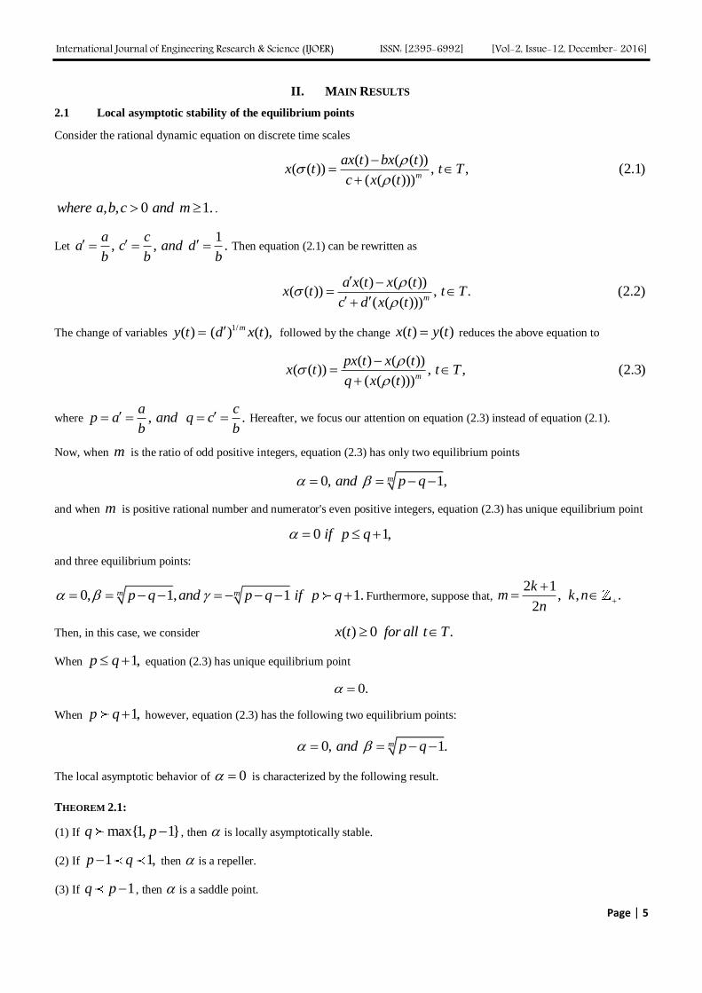
II. MAIN RESULTS

2.1 Local asymptotic stability of the equilibrium points

Consider the rational dynamic equation on discrete time scales

( ) ( ( ))( ( )) , , (2.1)

( ( ( )))m

ax t bx tx t t T

c x t

, , 0 1.where a b c and m .

Let 1

, , .a c

a c and db b b

Then equation (2.1) can be rewritten as

( ) ( ( ))( ( )) , . (2.2)

( ( ( )))m

a x t x tx t t T

c d x t

The change of variables 1/( ) ( ) ( ),my t d x t followed by the change ( ) ( )x t y t reduces the above equation to

( ) ( ( ))( ( )) , , (2.3)

( ( ( )))m

px t x tx t t T

q x t

where , .a c

p a and q cb b

Hereafter, we focus our attention on equation (2.3) instead of equation (2.1).

Now, when m is the ratio of odd positive integers, equation (2.3) has only two equilibrium points

0, 1,mand p q

and when m is positive rational number and numerator's even positive integers, equation (2.3) has unique equilibrium point

0 1,if p q

and three equilibrium points:

0, 1, 1 1.m mp q and p q if p q Furthermore, suppose that, 2 1

, , .2

km k n

n

Then, in this case, we consider ( ) 0 .x t for all t T

When 1,p q equation (2.3) has unique equilibrium point

0.

When 1,p q however, equation (2.3) has the following two equilibrium points:

0, 1.mand p q

The local asymptotic behavior of 0 is characterized by the following result.

THEOREM 2.1:

(1) If max{1, 1}q p , then is locally asymptotically stable.

(2) If 1 1,p q then is a repeller.

(3) If 1q p , then is a saddle point.


Page | 6

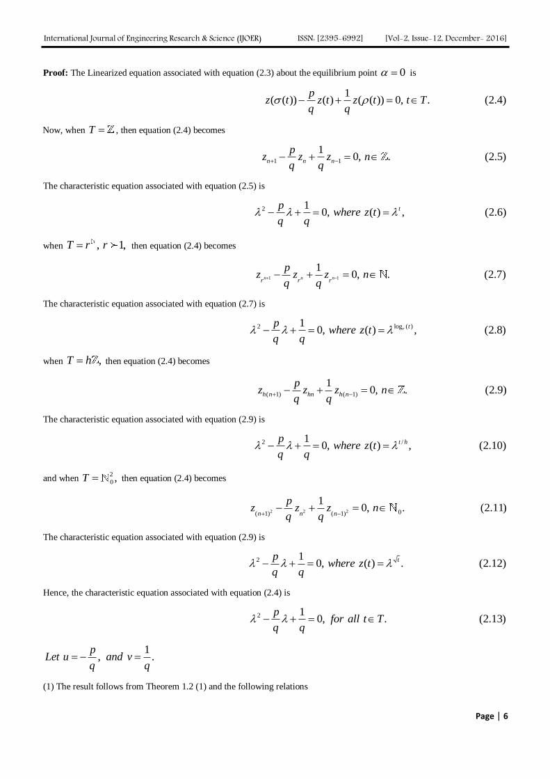
Proof: The Linearized equation associated with equation (2.3) about the equilibrium point 0 is

1( ( )) ( ) ( ( )) 0, . (2.4)

pz t z t z t t T

q q

Now, when T , then equation (2.4) becomes

1 1

10, . (2.5)n n n

pz z z n

q q


2 10, ( ) , (2.6)tp

where z tq q

when , 1,T r r then equation (2.4) becomes

1 1

10, . (2.7)n n nr r r

pz z z n

q q


log ( )2 10, ( ) , (2.8)r tp

where z tq q

when ,T h then equation (2.4) becomes

( 1) ( 1)

10, . (2.9)h n hn h n

pz z z n

q q


2 /10, ( ) , (2.10)t hp

where z tq q

and when 2

0 ,T then equation (2.4) becomes

2 2 2 0( 1) ( 1)

10, . (2.11)

n n n

pz z z n

q q


2 10, ( ) . (2.12)tp

where z tq q

Hence, the characteristic equation associated with equation (2.4) is

2 10, . (2.13)

pfor all t T

q q

1, .

pLet u and v

q q

(1) The result follows from Theorem 1.2 (1) and the following relations


Page | 7

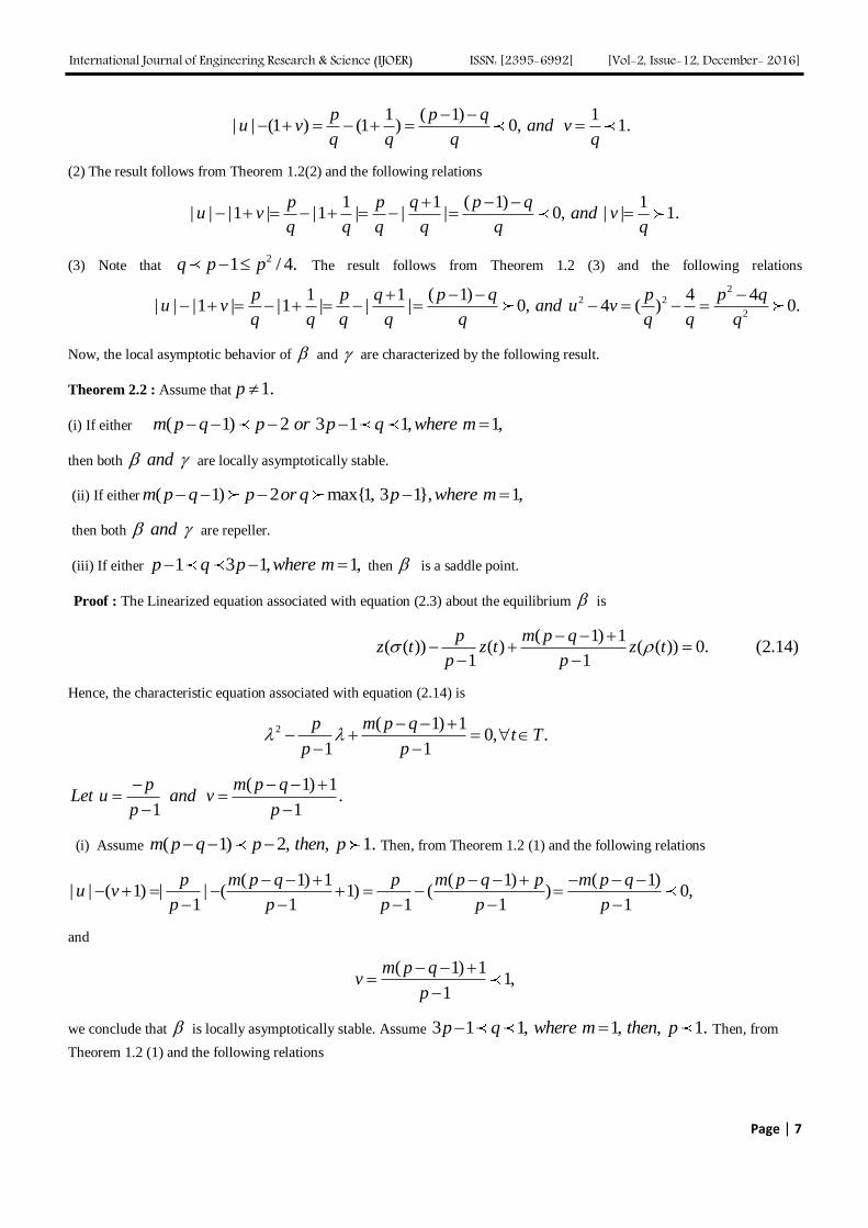
1 ( 1) 1| | (1 ) (1 ) 0, 1.

p p qu v and v

q q q q

(2)

The result follows from Theorem 1.2(2) and the following relations

1 1 ( 1) 1| | |1 | |1 | | | 0, | | 1.

p p q p qu v and v

q q q q q q

(3) Note that 21 / 4.q p p

The result follows from Theorem 1.2 (3) and the following relations

22 2

2

1 1 ( 1) 4 4| | |1 | |1 | | | 0, 4 ( ) 0.

p p q p q p p qu v and u v

q q q q q q q q

Now, the local asymptotic behavior of and are characterized by the following result.

Theorem 2.2 : Assume that 1.p

(i) If either ( 1) 2 3 1 1, 1,m p q p or p q where m

then both and are locally asymptotically stable.

(ii) If either ( 1) 2 max{1, 3 1}, 1,m p q p or q p where m

then both and are repeller.

(iii) If either

1 3 1, 1,p q p where m then is a saddle point.

Proof : The Linearized equation associated with equation (2.3) about the equilibrium is

( 1) 1( ( )) ( ) ( ( )) 0. (2.14)

1 1

p m p qz t z t z t

p p

Hence, the characteristic equation associated with equation (2.14) is

2 ( 1) 10, .

1 1

p m p qt T

p p

( 1) 1.

1 1

p m p qLet u and v

p p

(i) Assume ( 1) 2, , 1.m p q p then p Then, from Theorem 1.2 (1) and the following relations

( 1) 1 ( 1) ( 1)| | ( 1) | | ( 1) ( ) 0,

1 1 1 1 1

p m p q p m p q p m p qu v

p p p p p

and

( 1) 11,

1

m p qv

p

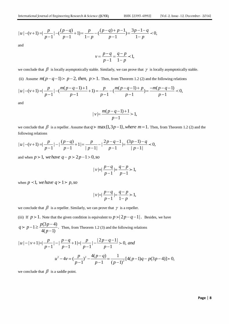
we conclude that is locally asymptotically stable. Assume 3 1 1, 1, , 1.p q where m then p Then, from

Theorem 1.2 (1) and the following relations


Page | 8

( ) ( ) 1 3 1| | ( 1) | | ( 1) ( ) 0,

1 1 1 1 1

p p q p p q p p qu v

p p p p p

and

1,1 1

p q q pv

p p

we conclude that is locally asymptotically stable. Similarly, we can prove that is locally asymptotically stable.

(ii) Assume ( 1) 2, , 1.m p q p then p Then, from Theorem 1.2 (2) and the following relations

( 1) 1 ( 1) ( 1)| | ( 1) | | ( 1) ( ) 0,

1 1 1 1 1

p m p q p m p q p m p qu v

p p p p p

and

( 1) 1| | 1,

1

m p qv

p

we conclude that is a repeller. Assume that max{1,3 1}, 1.q p where m Then, from Theorem 1.2 (2) and the

following relations

( ) 2 1 (3 1)| | ( 1) | | | 1| | | 0,

1 1 | 1| 1 | 1|

p p q p p q p qu v

p p p p p

and when 1, 2 1 0,p wehave q p p so

| | | | 1,1 1

p q q pv

p p

when 1, 1 ,p wehave q p so

| | | | 1,1 1

p q q pv

p p

we conclude that is a repeller. Similarly, we can prove that is a repeller.

(iii) If 1.p Note that the given condition is equivalent to | 2 1| .p p q Besides, we have

(3 4)1 .

4( 1)

p pq p

p

Then, from Theorem 1.2 (3) and the following relations

| 2 1|| | | 1| | | | 1| | | 0,

1 1 1 1

p p q p p qu v and

p p p p

2 2

2

4( ) 14 ( ) [4( 1) (3 4)] 0,

1 1 ( 1)

p p qu v p q p p

p p p

we conclude that is a saddle point.


Page | 9

Assume that 1.p Note that the given condition is equivalent to | 2 1| .p p q Besides, we have

(4 3 )3 1 .

4(1 )

p pq p

p

Then, from Theorem 1.2 (3) and the following relations

| 2 1|| | | 1| | | | 1| 0,

1 1 1 1

p p q p p qu v and

p p p p

2 2

2

4( ) 14 ( ) [ (4 3 ) 4(1 ) ] 0,

1 1 (1 )

p p qu v p p p q

p p p

we conclude that is a saddle point.

2.2 Boundedness of solutions of equation (2.3)

In this section, we study the boundedness of solution of equation (2.3).

Theorem 2.3: Suppose that 1p q and m is positive rational number and numerator's even positive integers,

1,2i . Then the solution of equation (2.3) is bounded for all t T .

Proof: We argue that | ( ) |x t A for all t T by induction on .t

Case (1): If T . Given any initial conditions 1 0| | | |x A and x A , we argue that | |nx A for all n by

induction on n . It follows from the given initial conditions that this assertion is true for 1,0.n Suppose the assertion is

true for 2 1( 1).n and n n That is,

2 1| | | | .n nx A and x A

Now, we consider nx , where we put n instead of ( 1)n in equation (2.3),

1 2 1 2

2 2 2

| | | | | | ( 1)| | (2.15)

| | | | | |

n n n nn m m m

n n n

px x p x x p Ax

q x q x q x

Since,

2 2

2

1 1| | 0, . (2.16)

| |

m m

n n m

n

q x q x qq x q

From (2.15) and (2.16), we obtain,

( 1)| | .n

p Ax A for all n

q

Case(2): If { : 0 }.T h hk h and k Given any initial conditions 0| | | |hx A and x A , we argue that

| |hnx A for all n by induction on n . It follows from the given initial conditions that this assertion is true for

1,0.n Suppose the assertion is true for 2 1( 1).n and n n That is,

( 2) ( 1)| | | | .h n h nx A and x A

Now, we consider hnx , where we put h n instead of ( 1)h n in equation (2.3),


Page | 10

( 1) ( 2) ( 1) ( 2)

( 2) ( 2) ( 2)

| | | | | | ( 1)| | . (2.17)

| | | | | |

h n h n h n h n

hn m m m

h n h n h n

px x p x x p Ax

q x q x q x

Since,

( 2) ( 2)

( 2)

1 1| | 0, . (2.18)

| |

m m

h n h n m

h n

q x q x qq x q


( 1)| | .hn

p Ax A for all n

q

Case (3): If 2 2

0 0{ : }.T n n Given any initial conditions 1 0| | | |x A and x A , we argue that

2

0| | ,kx A for all k n n by induction on k . It follows from the given initial conditions that this assertion is true

for 0,1.k Suppose the assertion is true for 2 2( 2) ( 1) .n and n That is,

2 2( 2) ( 1)| | | | .

n nx A and x A

Now, we consider 2nx , where we put n instead of ( 1)n in equation (2.3),

2 2 2 2

2

2 2 2

( 1) ( 2) ( 1) ( 2)

( 2) ( 2) ( 2)

| | | | | | ( 1)| | . (2.19)

| | | | | |

n n n n

m m mn

n n n

px x p x x p Ax

q x q x q x

Since, 2 2

2

( 2) ( 2)

( 2)

1 1| | 0, . (2.20)

| |

m m

mn n

n

q x q x qq x q


( 1)| | .k

p Ax A for all k

q

Case(4): If , 1T r r . Given any initial conditions 1/ 1| | | |rx A and x A , we argue that

| | ,n

kx A for all k r n by induction on k . It follows from the given initial conditions that this assertion is true

for 1/ ,1.k r Suppose the assertion is true for 2 1, .n nk r and k r where n That is,

2 1| | | | .n nr rx A and x A

Now, we consider 2rx , where we put n instead of ( 1)n in equation (2.3),

1 2

2 2

| | | | ( 1)| | . (2.21)

| | | |

n n

n

n n

r r

m mr

r r

p x x p Ax

q x q x

Since, 2 2

2

1 1| | , . (2.22)

| |n n

n

m m

mr r

r

pq x q x q

q x q


( 1)| | . completes the proof.k

p Ax A for all k This

q


Page | 11

2.3 Periodic solutions of equation

In this section, we study the existence of periodic solutions of equation (2.3).

The following theorem states the necessary and sufficient conditions that this equation has a periodic solutions.

Theorem 2.4: Equation (2.3) has prime period two solutions if and only if

23 1, 1.q p where q p p and m

Proof: First, suppose that, there exists a prime period two solution

..., , , , ,...,

of equation (2.3). We will prove that 3 1.q p

We see from equation (2.3) that

.p p

andq q

Then, 2 2, , ,q p and q p hence

( ) ( )( ) ( ) ( ).q p

Since, 0, ( ) 1 .q p Therefore,

( 1), (2.23)p q

and so,

2( ) ( ) ( )( ). , [ ( ) ] ( ).

( )( )

pq q pSince q q pq q p

q q

Hence,

( 1) ( )( ). (2.24)q p q p q

From (2.23) and (2.24), we obtain

( 1) ( )( 1). , ( 1). (2.25)q p q p q p q Then p p q

It is clear now, from equation (2.23) and (2.25) that and are the two distinct roots of the quadratic equation

2 ( 1) ( 1) 0,t p q t p p q

So,

( 1)( 1 3 ) 0. , 3 1.p q q p Then q p

Second, suppose that 3 1q p . We will show that equation (2.3) has a prime period two solutions. Assume that

( 1) ( 1)( 1 3 ) ( 1) ( 1)( 1 3 ), .

2 2

p q p q q p p q p q q pand

Therefore and are distinct real numbers. Set,

0 0 0( ( )) ( ) , .x t and x t t T

We wish to show that

0 0( ( )) ( ( )) .x t x t


Page | 12

It follows from equation (2.3) that

0 00

0

( ) ( ( ))( ( ))

( ( ))

[ ( 1) ( 1)( 1 3 ) [( 1) ( 1)( 1 3 )]

( 1) ( 1)( 1 3 ) ( 1) ( 1)( 1 3 )

( 1)(1 ) ( 1) ( 1)( 1 3 )

( 1) ( 1)( 1 3 )

( 1)(1

px t x tx t

q x t

p p q p q q p p q p q q p

q p p q q p q p p q q p

q p p p p q q p

q p p q q p

q p

2

2

2

2

0

) ( 1) ( 1)( 1 3 )[( 1) ( 1)( 1 3 )]

( 1) ( 1)( 1 3 )

2( )[( 1) ( 1)( 1 3 )]

4( )

( 1) ( 1)( 1 3 )( ( )) , .

2

p p p q q pq p p q q p

q p p q q p

p p q p q p q q p

p p q

p q p q q px t q p p

Similarly as before one can easily show that

( ( )) , ( ( )) ( ) .x t where x t and x t

Thus equation (2.3) has the prime period two solution

..., , , , ,...,

where and are the distinct roots of the quadratic equation (2.3). The proof is completed.

To examine the global attractivity of the equilibrium points of equation (2.3), we first need to determine the invariant

intervals for equation (2.3).

2.4 Invariant intervals and global attractivity of the zero equilibria

In this subsection, we determine the family of invariant intervals centered at 0.

Theorem 2.5: Assume 1q p . Then for any positive real number

1/( ( 1)) ,mA q p

The interval (0, ) ( , )O A A A is invariant for eq. (2.3).

Proof: We consider 2 2

0 0, { : 0 }, { : }, , 1.T h hk h and k n n and r r

Case (1): If T . Given any initial conditions 1 0| | | |x A and x A ,we argue that | |nx A for all n by

induction on n . It follows from the given initial conditions that this assertion is true for 1,0.n Suppose the assertion is

true for 2 1( 1).n and n n That is,

1/ 1/

2 1| | ( ( 1)) , | | ( ( 1)) .m m

n nx A q p and x A q p

Now, we consider nx , where we put n instead of ( 1)n in equation (2.3). Since,

2 ( ( 1)) 1 0,m m

nq x q A q q p p


Page | 13

2

11. (2.26)

| |m

n

p

q x

Thus,

1 2 1 21 2

2 2 2

1 2

| | | | | | 1| | ( ) max{| |,| |}

| | | | | |

max{| |,| |} .

n n n nn n nm m m

n n n

n n

px x p x x px x x

q x q x q x

x x A for all n

Case (2): If { : 0 }.T h hk h and k Given any initial conditions 0| | | |hx A and x A , we argue that

| |hnx A for all n by induction on n . It follows from the given initial conditions that this assertion is true for

,0.n h Suppose the assertion is true for 2 1( 1).n and n n That is,

1/ 1/

( 2) ( 1)| | ( ( 1)) , | | ( ( 1)) .m m

h n h nx A q p and x A q p

Now, we consider hnx , where we put h n instead of ( 1)h n in equation (2.3). Since,

( 2) ( ( 1)) 1 0,m m

h nq x q A q q p p

( 2)

11. (2.27)

| |m

h n

p

q x

Thus,

( 1) ( 2) ( 1) ( 2)

( 1) ( 2)

( 2) ( 2) ( 2)

( 1) ( 2)

| | | | | | 1| | ( ) max{| |,| |}

| | | | | |

max{| |,| |} .

h n h n h n h n

hn h n h nm m m

h n h n h n

h n h n

px x p x x px x x

q x q x q x

x x A for all n

Case (3): If 2 2

0 0{ : }.T n n Given any initial conditions 1 0| | | |x A and x A , we argue that

2

0| | ,kx A for all k n n by induction on k . It follows from the given initial conditions that this assertion is true

for 0,1.k Suppose the assertion is true for 2 2( 2) ( 1) .n and n That is,

2 2

1/ 1/

( 2) ( 1)| | ( ( 1)) , | | ( ( 1)) .m m

n nx A q p and x A q p

Now, we consider 2nx , where we put n instead of ( 1)n in equation (2.3). Since,

2( 2)( ( 1)) 1 0,m m

nq x q A q q p p

2( 2)

11. (2.28)

| |m

n

p

q x

Thus,

2 2 2 2

2 2 2

2 2 2

2 2

( 1) ( 2) ( 1) ( 2)

( 1) ( 2)

( 2) ( 2) ( 2)

2

( 1) ( 2)

| | | | | | 1| | ( ) max{| |,| |}

| | | | | |

max{| |,| |} .

n n n n

m m mn n n

n n n

n n

px x p x x px x x

q x q x q x

x x A for all k n


Page | 14

Case (4): If , 1T r r . Given any initial conditions 1/ 1| | | |rx A and x A , we argue that

| | ,n

kx A for all k r n by induction on k . It follows from the given initial conditions that this assertion is true

for 1/ ,1.k r Suppose the assertion is true for 2 1, .n nk r and k r where n That is,

2 1

1/ 1/| | ( ( 1)) , | | ( ( 1)) .n n

m m

r rx A q p and x A q p

Now, we consider 2rx , where we put n instead of ( 1)n in equation (2.3). Since,

2 ( ( 1)) 1 0,n

m m

rq x q A q q p p

2

11. (2.29)

| |n

m

r

p

q x

Thus,

1 2 1 2

1 2

2 2 2

1 2

| | | | | | 1| | ( ) max{| |,| |}

| | | | | |

max{| |,| |} . This completes the proof.

n n n n

n n n

n n n

n n

r r r r

m m mr r r

r r r

r r

px x p x x px x x

q x q x q x

x x A for all n

Now, we investigate the global attractivity of the equilibrium point 0.

Lemma 2.1: Assume that , 1,T q p and m is positive rational number and numerator's even positive integers.

Furthermore, suppose that

1( ( 1)) , (2.30)lmR q p

and consider equation (2.3) with the restriction that

: (0, ) (0, ) (0, ).f O R O R O R

Let { }nx be a solution of this equation and

1

1 0

1. (2.31)

(max{| |,| |})m

pR

q x x

Then, 1 (0,1),R and

/ 2

1 1 0| | max{| |,| |}, 1,2,... . (2.32)n

nx R x x n

Proof: From Theorem 2.5, we have

| | , 1,0,1,2,... ,nx A R n

where we put n instead of ( 1)n in equation (2.3). Then, 1 0(max{| |,| |}) .m mx x R

Thus,

1 0(max{| |,| |}) 1 0.m mq x x q R p

Hence,


Page | 15

1

1 0

10 1. (0,1).

(max{| |,| |})m

pThis means that R

q x x

Now, we prove that (2.32), by induction on n . From equation (2.3), we have

1 2 1 2

2 2

1 2

1 1| | ( | | | |) ( ) max{| |,| |} (2.33)

| | | |

max{| |,| |}, (2.26). (2.34)

n n n n nm m

n n

n n

px p x x x x

q x q x

x x from

Then, from (2.33), we obtain

1 0 1

1

1| | ( ) max{| |,| |}. (2.35)

| |m

px x x

q x

But

1 0 1

1 0 1

| | (max{| |,| |}) 1 0. ,

| | (max{| |,| |}) 0.

m m m

m m

q x q x x q R p Then

q x q x x

From (2.35), we have

1 0 1 0 1

1 0 1

1/ 2

1 0 1 1 0 1

1 1| | ( ) max{| |,| |} max{| |,| |}

| | (max{| |,| |})

max{| |,| |} max{| |,| |},

m m

p px x x x x

q x q x x

R x x R x x

and from (2.33) and (2.34), we obtain

2 1 0 1 0

0 1 0

0 1 0

0 1 0

1 0 1 1 0

1 0

1 1| | ( ) max{| |,| |} max{| |,| |}

| | (max{| |,| |})

1max{max{| |,| |},| |}

(max{max{| |,| |},| |})

1max{| |,| |} max{| |,| |}.

(max{| |,| |})

m m

m

m

p px x x x x

q x q x x

px x x

q x x x

px x R x x

q x x

Thus, the inequality (2.32) holds for 1,2.n Suppose that the inequality (2.32) holds for 1n and 2( 3)n n ,

respectively. By (2.34), we have

0 1| | max{| |,| |} .nx x x for all n

So,

1

2 2 0 1

1 1 10 .

| | | | (max{| |,| |})m m m

n n

p p pR

q x q x q x x

Then, from (2.33), we have

1 2 1 1 2

2

( 1) / 2 ( 2) / 2 / 2

1 1 1 0 1 1 0 1

1| | ( ) max{| |,| |} max{| |,| |}

| |

max{ , } max{| |,| |} max{| |,| |}.

n n n n nm

n

n n n

px x x R x x

q x

R R R x x R x x


Page | 16

This completes the inductive proof of (2.32).

Lemma 2.2: Assume that { : (0,1) }, 1,T h hk h and k q p and m is positive rational number and

numerator's even positive integers. Furthermore, suppose that (2.30) holds and consider equation (2.3) with the restriction

that

: (0, ) (0, ) (0, ).f O R O R O R

Let { : (0,1) }knx h and n be a solution of this equation and

1

0

1. (2.36)

(max{| |,| |})m

h

pR

q x x

Then, 1 (0,1),R and / 2

1 0| | max{| |,| |}, 1,2,... . (2.37)hn

hn hx R x x n


| | , 1,0,1,... ,hnx A R n

Where we put hn instead of ( 1)h n in equation (2.3). Then, 0(max{| |,| |}) .m m

hx x R Thus,

0(max{| |,| |}) 1 0.m m

hq x x q R p Hence,

1

0

10 1. (0,1).

(max{| |,| |})m

h

pThis means that R

q x x


( 1) ( 2)

( 1) ( 2)

( 2) ( 2)

( 1) ( 2)

| | | | 1| | ( ) max{| |,| |} (2.38)

| | | |

max{| |,| |}, (2.27). (2.39)

h n h n

hn h n h nm m

h n h n

h n h n

p x x px x x

q x q x

x x from


0

1| | ( ) max{| |,| |}. (2.40)

| |h hm

h

px x x

q x

But

0 0| | (max{| |,| |}) 1 0. , | | (max{| |,| |}) 0.m m m m m

h h h hq x q x x q R p Then q x q x x


0 0

0

/ 2

1 0 1 0

1 1| | ( ) max{| |,| |} max{| |,| |}

| | (max{| |,| |})

max{| |,| |} max{| |,| |},

h h hm m

h h

h

h h

p px x x x x

q x q x x

R x x R x x



Page | 17

2 0 0

0 0

0 0

0 0

0 1 0

0

2 / 2

1

1 1| | ( ) max{| |,| |} max{| |,| |}

| | (max{| |,| |})

1max{max{| |,| |},| |}

(max{max{| |,| |},| |})

1max{| |,| |} max{| |,| |}

(max{| |,| |})

max{

h h hm m

h

hm

h

h hm

h

h

p px x x x x

q x q x x

px x x

q x x x

px x R x x

q x x

R

0| |,| |}.hx x

Thus, the inequality (2.37) holds for 1,2.n Suppose that the inequality (2.37) holds for ( 1)h n and ( 2)( 3)h n n ,


0| | max{| |,| |} .n hx x x for all n

So,

1

( 2) ( 2) 0

1 1 10 .

| | | | (max{| |,| |})m m m

h n h n h

p p pR

q x q x q x x


1 1

( 1) ( 2) 1 ( 1) ( 2)

( 2)

( 1) / 2 ( 2) / 2

( 1) ( 2) 1 1 0

/ 2

1 0

1| | ( ) max{| |,| |} max{| |,| |}

| |

max{| |,| |} max{ , } max{| |,| |}

max{| |,| |}.

hn h n h n h n h nm

h n

h h h n h n

h n h n h

hn

h

px x x R x x

q x

R x x R R R x x

R x x


Lemma 2.3: Assume that 2 2

0 0{ : }, 1,T n n q p and m is positive rational number and numerator's even

positive integers. Furthermore, suppose that (2.30) holds and consider equation (2.3) with the restriction that

: (0, ) (0, ) (0, ).f O R O R O R

Let 2

0{ : }kx k n and n be a solution of this equation and

1

1 0

1. (2.41)

(max{| |,| |})m

pR

q x x

Then,

/ 2

1 1 0| | max{| |,| |}, 1,4,... . (2.42)k

kx R x x k


| | , 1,2,... ,kx A R k

where we put n instead of ( 1)n in equation (2.3). Then, 1 0(max{| |,| |}) .m mx x R

Thus,

1 0(max{| |,| |}) 1 0.m mq x x q R p

Hence,


Page | 18

1

1 0

10 1. (0,1).

(max{| |,| |})m

pThis means that R

q x x

Now, we prove that (2.42), by induction on k . From equation (2.3), we have

2 2

2

2

2 2

2

2 2

( 1) ( 2)

( 2)

( 1) ( 2)

( 2)

( 1) ( 2)

| | | || |

| |

1( ) max{| |,| |} (2.43)| |

max{| |,| |}, (2.28). (2.44)

n n

mn

n

m n n

n

n n

p x xx

q x

px x

q x

x x from


1 0 1

1

1| | ( ) max{| |,| |}. (2.45)

| |m

px x x

q x

But

1 1 0 1| | | | (max{| |,| |}) 1 0. ,m m m mq x q x q x x q R p Then

1 0 1| | (max{| |,| |}) 0.m mq x q x x


1 0 1 0 1

1 0 1

1/ 2

1 0 1 1 0 1

1 1| | ( ) max{| |,| |} max{| |,| |}

| | (max{| |,| |})

max{| |,| |} max{| |,| |},

m m

p px x x x x

q x q x x

R x x R x x


1

4 1 0 1 0

0 1 0

1 0 1 0

0 1 0

2

1 1 0 1 0

1 0

4/ 2

1

1 1| | ( ) max{| |,| |} max{| |,| |}

| | (max{| |,| |})

1max{ max{| |,| |},| |}

(max{max{| |,| |},| |})

1max{| |,| |} max{| |,| |}

(max{| |,| |})

max{|

m m

m

m

p px x x x x

q x q x x

pR x x x

q x x x

pR x x R x x

q x x

R

1 0|,| |}.x x

Thus, the inequality (2.42) holds for 1, 2.n Suppose that the inequality (2.42) holds for 2( 1)n and

2( 2)n ,


2 2 2 0( 1) ( 2)| | max{| |,| |} .

n n nx x x for all n


Page | 19

2 2

1

0 1( 2) ( 2)

1 1 1, 0 .

| | | | (max{| |,| |})m m m

n n

p p pSo R

q x q x q x x


2 2 2 2 2

2

2 2 2

2

1( 1) ( 2) ( 1) ( 2)

( 2)

( 1) / 2 ( 2) / 2 ( 2) / 2

1 1 0 1 1 0 1

/ 2

1 0 1

1| | ( ) max{| |,| |} max{| |,| |}

| |

max{ , } max{| |,| |}} max{| |,| |}, 3,4,...

max{| |,| |}, 1,2,... .

mn n n n n

n

n n n

n

px x x R x x

q x

R R x x R x x n

R x x n


Lemma 2.4: Assume that , 1 2, 1,T r r q p and m is positive rational number and numerator's even

positive integers. Furthermore, suppose that (2.30) holds and consider equation (2.3) with the restriction that

: (0, ) (0, ) (0, ).f O R O R O R

Let { : , 1 2}n

kx k r n and r be a solution of this equation and

1

1/ 1

1. (2.46)

(max{| |,| |})m

r

pR

q x x

Then, 1 (0,1),R and / 2

1 1/ 1| | max{| |,| |}. (2.47)k

k rx R x x


| | , , , 1 2,n

kx A R k r n and r

where we put n instead of ( 1)n in equation (2.3). Then, 1/ 1(max{| |,| |}) .m m

rx x R Thus,

1/ 1(max{| |,| |}) 1 0. ,m m

rq x x q R p Hence 1/ 1

10 1.

(max{| |,| |})m

r

pThis means that

q x x

1 (0,1).R


1 2

2

1 2

2

1 2

1| | ( | | | |)

| |

1( ) max{| |,| |} (2.48)| |

max{| |,| |}, (2.29). (2.49)

n n n

n

n n

n

n n

mr r r

r

m r r

r

r r

x p x xq x

px x

q x

x x from


1/ 1

1/

1| | ( ) max{| |,| |}. (2.50)

| |r rm

r

px x x

q x

But


Page | 20

1/ 1/ 1/ 1| | | | (max{| |,| |}) 1 0. ,m m m m

r r rq x q x q x x q R p Then

1/ 1/ 1/ 1| | | | (max{| |,| |}) 0.m m m

r r rq x q x q x x


1/ 1 1/ 1

1/ 1/ 1

/ 2

1 1/ 1 1 1/ 1

1 1| | ( ) max{| |,| |} max{| |,| |}

| | (max{| |,| |})

max{| |,| |} max{| |,| |},

r r rm m

r r

r

r r

p px x x x x

q x q x x

R x x R x x


2 1 1

1 1

/ 2

1 1/ 1 1

1/ 1 1

/ 2 / 2

1 1/ 1 1 1

1/ 1

1 1| | ( ) max{| |,| |} max{| |,| |}

| | (max{| |,| |})

1max{ max{| |,| |},| |}

(max{max{| |,| |},| |})

1max{| |,| |} max{|

(max{| |,| |})

r rm mrr

r

rm

r

r r

rm

r

p px x x x x

q x q x x

pR x x x

q x x x

pR x x R R x

q x x

2

1/ 1

2 / 2 / 2

1 1/ 1 1 1/ 1

|,| |}

max{| |,| |} max{| |,| |}.

r

r r

r r

x

R x x R x x

Thus, the inequality (2.47) holds for 2, .k r r Suppose that the inequality (2.47) holds for

2 1, ,n nk r and k r n respectively. By (2.49), we have

1 2| | max{| |,| |} .n n nr r rx x x for all n

So,

2 2

1

1/ 1

1 1 10 .

| | | | (max{| |,| |})n n

m m m

rr r

p p pR

q x q x q x x


1 2 1 2

2

1 2

2

1

/ 2 / 2

1 1/ 1 1 1/ 1

/ 2

1 1/ 1

/ 2

1 1/ 1

1| | ( ) max{| |,| |} max{| |,| |}

| |

max{ max{| |,| |}, max{| |,| |}}

max{| |,| |}}, 3,4,...

max{| |,| |}, 1,2,3,... .

n n n n n

n

n n

n

n

mr r r r r

r

r r

r r

r

r

r

r

px x x R x x

q x

R x x R x x

R x x n

R x x n


Theorem 2.6: Assume that 1,q p and m is positive rational number and numerator's even positive integers.

Furthermore, suppose that (2.30) holds, and consider equation (2.3) with the restriction that

: (0, ) (0, ) (0, ).f O R O R O R

Then the equilibrium point 0 of the equation (2.3) is a global attractor.


Page | 21

Proof: From Lemmas 2. , 1,2,3,4, ( ) 0 ,i i x t when t then the equilibrium point 0 of the equation

(2.3) is a global attractor.

Next, we determine the family of invariant intervals centered at 1, 1.m p q where p q

2.5 Invariant intervals and global attractivity of the nonzero equilibria

In this subsection, we consider the discrete time scales

, { : 0 },T h hk h and k 2 2

0 0{ : },n n , 1, 1and r r m . This means that, we determine

the family of invariant intervals centered at 1.p q To this end, we establish the following relation.

( ) ( ( )) ( )( ( )) ( 1) ( 1)

( ( )) ( ( ))

( ) ( )( ) ( )

( ( )) ( ( )) ( ( )) ( ( ))

( ( ) ) ( ( (( ( )) ( ( ( )))( )

px t x t p px t q p qx t

q x t q q x t q

px t q p q px t q p q p q p q

q x t q q x t q x t q x t q

p p qx t x

q x t q x t q

)) ).t

In view of (1 )( ) ( )( ),p q q p q q the above equality is reduced to

( ( )) ( ( ) ) ( ( ( )) ). ,( ( )) ( ( ))

p q px t x t x t Thus

q x t q x t

| || ( ( )) | | ( ) |) | ( ( )) |

( ( )) ( ( ))

| |max{| ( ( )) |,| ( ) |}. (2.51)

( ( ))

p q px t x t x t

q x t q x t

p p qx t x t

q x t

Now, we are ready to describe the family of nested invariant intervals centered at .

Theorem 2.7: Assume that 1/ 2, 3 1 1 .p and p q p Then for every positive number

min{ (3 1),(1 ) ,1 2 }, (2.52)A q p p q p

the interval

( , ) ( , )O A A A

is invariant for equation (2.3).

Proof: Case (1): If T , given any initial conditions

1 0| | | | ,x A and x A

we argue that

| | .nx A for all n byinductionon n

The proof is similar to the proof of Theorem 4.2 in [24 ] and will be omitted.

Case 2: If T h , given any initial conditions

0| | | | ,hx A and x A


Page | 22

we argue that

| | .hnx A for all n byinductionon n

It follows from the given initial assertion is true for 1,0.n Suppose the asseration is true for

( 2) ( 1).h n and h n That is,

( 2) ( 1)| | | | .h n h nx A and x A

Now, we consider hnx where we put hn instead of ( 1)h n in equation (2.51). Since,

( 2)

( 2) ( 2)

( ) ( 1) (1 ) (1 ) 0,

| | ( ). , (1 2 )

( ) (1 2 ) 0,

h n

h n h n

q x q A q p q A A p A p

wehave q x q x Now thecondition A q p is equivalent to

q A p p A

( 2) ( 2)

(3 1)

( ( ) ),

(1 )

( ( ) ).

, | | ( ( ) ). ,

| | ( | |) ( ) | |

( ) | | (

h n h n

the condition A q p is equivalent to

p q q A p

and the condition A p q is equivalent to

p q q A p

So p q q A p Thus

q x p p q q x p p q

q A p p q q

) ( ) 0.A p q A p

From this we deduce that

( 2)

| |1.

| |h n

p p q

q x

By (2.51), we have

( 1) ( 2)

( 2)

( 1) ( 2)

| || | max{| |,| |}

| |

max{| |,| |} .

hn h n h n

h n

h n h n

p p qx x x

q x

x x A

This completes the inductive proof.

When 2

0 , 1,T and r r the proof will be omitted.

Now, we investigate the global attractivity of the equilibrium point .

Lemma 2.8: Assume that , 1/ 2, 3 1 1 .T p and p q p Consider equation (2.3) with the restriction that

: ( , ) ( , ) ( , ),f O R O R O R where

min{ (3 1),(1 ) ,1 2 }. (2.53)R q p p q p

Let { }nx be a solution of this equation and

1 0

| |. (2.54)

1 max{| |,| |}

p p qM

p x x


Page | 23

Then, (0,1),M and

/ 2

1 0| | max{| |,| |}, 1,2,... (2.55)n

nx M x x n

The proof is similar to the proof of Lemma 6.1 in [24 ] and will be omitted.

Lemma 2.9: Assume that { : (0,1) }, 1/ 2,T h hk h and k p 3 1 1 ,and p q p and (2.53)

holds. Consider equation (2.3) with the restriction that

: ( , ) ( , ) ( , ).f O R O R O R

Let { : (0,1) }hnx h and n be a solution of this equation and

0

| |. (2.56)

1 max{| |,| |}h

p p qM

p x x

Then, (0,1),M and

/ 2

0| | max{| |,| |}, 1,2,...(2.57)hn

hn hx M x x n

Proof: Note that

1 | | ( | |) 1 ( | |) 1 2 | | .

, ,

1 | | ( | |) ( (3 1)) 0.

h

h

p x p p q p R p p q p p q R

When p q

p x p p q q p R

, , 1 | | ( | |) ((1 ) ) 0.hWhen p q p x p p q p q R

| |, 0 1.

1 | |

| |, 0 1. , (0,1).

1 | |

h

h

p p qSo

p x

p p qSimilarly Hence M

p x

Next, we prove equation (2.57) by induction on n. By (2.51), where we put hn instead of ( 1)h n , we

have0

| || | max{| |,| |}.h h

h

p p qx x x

q x

Since,

0

0

0

0

( _ ( ) 1 ( ) 1 max{| |,| |}

1 (1 2 ) 0,

| | | |0.

1 max{| |,| |}

,

| |0. ,

| | max{| |,| |}

h h h h

h h

h h

q x q x p x p x x

p R p R we derive

p p q p p qM

p x x q x

Similarly we have

p p qM Then

q x

x M x x M

/ 2

0max{| |,| |}.h

hx x

And we have,


Page | 24

2 0

0

0 0

0

2 / 2

0

| || | max{| |,| |}

max{| |, max{| |,| |}}

max{| |,| |}

max{| |,| |}.

h h

h

h

h

h

p p qx x x

q x

M x M x x

M x x

M x x

So equation (2.57) holds for 1,2. Suppose that equation (2.57) holds for ( 1) ( -2), respectively.

By(2.51) and the inductive hypothesis, we have

n h n and h n

( 1) ( 2)

( 2)

( 1) / 2 ( 2) / 2

0

( 2)

| || | max{| |,| |}

| |max{ , } max{| |,| |}}.

, (2.7),

hn h n h n

h n

h n h n

h

h n

p q px x x

q x

p q pM M x x

q x

Now fromTheorem we have

( 1) ( 2)

0

| | max{| |,| |}.

,

| | max{| |,| |}, ,

hn h n h n

hn h

x x x

By inductionon n wecan prove

x x x hence

( 2) ( 2) ( 2)

0

( 2)

( ) ( ) 1 ( )

1 max{| |,| |} 1 (1 2 ) 0,

| |0 ,

h n h n h n

h

h n

q x q x p x

p x x p R p R

p q pweconclude M then

q x

( 1) / 2 ( 2) / 2

0

/ 2 ( 1) / 2 ( 2) / 2

0

/ 2 / 2

0

/ 2

0

| | max{ , } max{| |,| |}}

max{ , } max{| |,| |}}

max{ ,1} max{| |,| |}}

max{| |,| |}}.

h n h n

hn h

h h n h n

h

nh h

h

nh

h

x M M M x x

M M M x x

M M x x

M x x

This completes the inductive proof of equation (2.57).

Lemma 2.10: Assume that 2 2

0 0{ : },T n n 1/ 2, 3 1 1 ,p and p q p and (2.53) holds. Consider

equation (2.3) with the restriction that

: ( , ) ( , ) ( , ).f O R O R O R

Let 2

0{ : }kx k n and n be a solution of this equation and

1 0

| |. (2.58)

1 max{| |,| |}

p p qM

p x x

Then, (0,1)M and

/ 2

1 0| | max{| |,| |}, 1,4,... . (2.59)k

kx M x x k


Page | 25

Lemma 2.11: Assume that , 1 2,T r r 1/ 2, 3 1 1 ,p and p q p and (2.53) holds. Consider equation

(2.3) with the restriction that

: ( , ) ( , ) ( , ).f O R O R O R

Let { : , 1 2, }n

kx k r r and n be a solution of this equation and

1/ 1

| |. (2.60)

1 max{| |,| |}r

p p qM

p x x

Then, (0,1)M and

/ 2

1/ 1| | max{| |,| |}. (2.61)k

k rx M x x

Theorem 2.9: Assume that 1/ 2, 3 1 1 ,p and p q p and (2.53) holds. Consider equation (2.3) with the

restriction that

: ( , ) ( , ) ( , ).f O R O R O R

Then the equilibrium point of the equation (2.3) is a global attractor.

Proof: From Lemmas 2. , 8,9,10,11, ( ) ,i i we obtain x t when t then the equilibrium point β of the

equation (2.3) is a global attractor.

ACKNOWLEDGEMENTS I thank my teacher Prof. E. M. Elabbasy.

REFERENCES

[1] M. T. Aboutaleb, M. A. El-Sayed and A. H. Hamza, Stability of the recursive sequence 1

1+

nn

n

xx

x

, Journal of

Mathematical Analysis and Applications, 261(2001), 126-133.

[2] R. P. Agarwal, M. Bohner, D. O'Regan and A. Peterson, Dynamic equations on time scales: A survey, J. Comp. Appl.

Math., Special Issue on (Dynamic Equations on Time Scales), edited by R. P. Agarwal, M. Bohner and D. O'Regan,

(Preprint in Ulmer Seminare 5)141(1-2) (2002), 1-26.

[3] A. M. Amleh, E. A. Grove and G. Ladas, On the recursive sequence 11

nn

n

xx

x

, Journal of Mathematical

Analysis and Applications, 233(1999), 790-798.

[4] M. Bohner and A. Peterson, Dynamic Equations on Time Scale, An Introduction with Applications, Birkhauser, Boston, 2001.

[5] M. Bohner and A. Peterson, First course on dynamic equations on time scales, August 2007.

[6] C. Cinar, On the positive solutions of the difference equation 11

11+

nn

n n

xx

x x

, Applied Mathematics and Computation,

150(2004), 21-24.

[7] K. Cunningham, M. R. S. Kulenovic, G. Ladas and S. V. Valicenti, On the recursive sequence 1

1B

nn

n n

xx

x Cx

,

Nonlinear Analysis, 47(2001), 4603-4614.

[8] O. Dosly and S. Hilger, A necessary and sufficient condition for oscillation of the Sturm-Liouville dynamic equation on

time scales, Special Issue on (Dynamic Equations on Time Scales), edited by R. P. Agarwal, M. Bohner and D. O'Regan,

J. Comp. Appl. Math. 141(1-2) (2002), 147-158.


Page | 26

[9] M. M. El- Afifi, On the recursive sequence 11

1B

n nn

n n

x xx

x Cx

, Applied Mathematics and Computation,

147(2004), 617-628.

[10] E. M. Elabbasy, H. El-Metwally and E. M. Elsayed, On the difference equation 1

1

nn n

n n

bxx ax

cx dx

, Adv.

Differ. Equ., Volume 2006, Article ID 82579,1--10.

[11] H. M. El-Owaidy and M. M. El- Afifi, A note on the periodic cycle of 12

1 nn

n

xx

x

, Applied Mathematics and

Computation, 109(2000), 301-306.

[12] H. M. El-Owaidy, A. M. Ahmed and M. S. Mousa, On the recursive sequences 11

nn

n

xx

x

, Applied Mathematics

and Computation, 145(2003), 747-753.

[13] Sh. R. Elzeiny, On the Rational Dynamic Equation on Discrete Time

Scales

1 2

( ( )) , T( ( )) ( ( ( )))

m m

ax t bx tx t t

c d x t x t

, IJOER, Vol. 1, Issue-6, Sept. -2015.

[14] C. Gibbons, M. R. S. Kulenovic and G. Ladas, On the recursive sequence 11

nn

n

xx

x

, Mathematical Sciences

Research Hot-Line, 4 (2)(2000), 1-11.

[15] S. Hilger, Analysis on measure chains- a unified approach to continuous and discrete calculus, Results Math. 18 (1990),

18-56.

[16] V. L. Kovic, G. Ladas and I. W. Rodrigues, On rational recursive sequences, Journal of Mathematical Analysis and Applications, 173(1993), 127-157.

[17] V. L. Kovic and G. Ladas, Global Behavior of Nonlinear Difference Equations of Higher Order with Applications,

Kluwer-Academic Publishers, Dordrecht, 1993.

[18] W. A. Kosmala, M. R. S. Kulenovic, G. Ladas and C. T. Teixeira, On the recursive sequence 11

1

nn

n n

p yy

qy y

,

Journal of Mathematical Analysis and Applications, 251(2000), 571-586.

[19] M. R. S. Kulenovic, G. Ladas and N. R. Prokup, A rational difference equation, Computers and Mathematics with

Applications, 41(2001), 671-678.

[20] W. Li and H. Sun, Global attractivity in a rational recursive sequence, Dynamic systems and applications 11 (2002), 339-346.

[21] X. Yan and W. Li, Global attractivity in the recursive sequence 1

1

nn

n

xx

x

, Applied Mathematics and

Computation, 138(2003), 415-423.

[22] X. Yan and W. Li, Global attractivity in a rational recursive sequence, Applied Mathematics and Computation,

145(2003), 1-12.

[23] X. Yang, H. Lai, David J. Evans and G. M. Megson, Global asymptotic stability in a rational recursive sequence,

Applied Mathematics and Computation,.158(2004), 703--716.

[24] X. Yang, B. Chen, G. M. Megson and D. J. Evans, Global attractivity in a recursive sequence, Applied Mathematics and Computation, 158(2004), 667--682.

[25] X. Yang, W. Su, B. Chen, G. M. Megson and D. J. Evans, On the recursive sequence 1 2

1 2

n nn

n n

ax bxx

c dx x

, Applied

Mathematics and Computation, 162(2005), 1485-1497.

[26] D. Zhang, B. Shi and M. Cai, A rational recursive sequence, Computers and Mathematics with Applications 41 (2001),

301-306.