st louis fed

A Measure of Price Pressures

Laura E. Jackson, Kevin L. Kliesen, and Michael T. Owyang

T he Federal Reserve, like most central banks, devotes considerable economic resourcesto monitoring and analyzing large volumes of economic data. This effort, often termed“current analysis” by insiders, feeds directly into another, crucial aspect of central

banking: forecasting key economic series such as real gross domestic product (GDP) growth,inflation, and employment. Forecasting the paths of key economic variables is an effort thatflows directly from the Fed’s congressionally mandated responsibility to (i) provide sufficientliquidity to achieve and maintain low inflation rates and (ii) promote maximum sustainableeconomic growth. This responsibility, which stems from the Federal Reserve Act and subse-quent amendments, is often termed the Fed’s dual mandate. Since the passage of the Dodd-Frank Wall Street Reform and Consumer Protection Act, the Fed has been handed a thirdmonetary policy responsibility: financial stability.

In this analysis, we focus on the Fed’s price stability mandate—specifically, in the contextof forecasting inflation. Given its importance, Federal Reserve officials have historically beenreluctant to attach an explicit definition of price stability—a rather ambiguous term that can

The Federal Reserve devotes significant resources to forecasting key economic variables such as realgross domestic product growth, employment, and inflation. The outlook for these variables also mattersa great deal to businesses and financial market participants. The authors present a factor-augmentedBayesian vector autoregressive forecasting model that significantly outperforms both a benchmarkrandom walk model and a pure time-series model. They then use these factors in an ordered probitmodel to develop the probability distribution over a 12-month horizon. One distribution assesses theprobability that inflation will exceed 2.5 percent over the next year; they term this probability a pricepressure measure. This price pressure measure would provide policymakers and markets with a quan-titative assessment of the probability that average inflation over the next 12 months will be higher thanthe Fed’s long-term inflation target of 2 percent. (JEL C32, C35, E31)

Federal Reserve Bank of St. Louis Review, First Quarter 2015, 97(1), pp. 25-52.

Laura E. Jackson will join the faculty in the department of economics at Bentley University as an assistant professor in July 2015. Kevin L. Kliesenand Michael T. Owyang are research officers and economists at the Federal Reserve Bank of St. Louis. The authors benefited from conversationswith Neville Francis. Lowell Ricketts and E. Katarina Vermann provided research assistance.

© 2015, The Federal Reserve Bank of St. Louis. The views expressed in this article are those of the author(s) and do not necessarily reflect the viewsof the Federal Reserve System, the Board of Governors, or the regional Federal Reserve Banks. Articles may be reprinted, reproduced, published,distributed, displayed, and transmitted in their entirety if copyright notice, author name(s), and full citation are included. Abstracts, synopses, andother derivative works may be made only with prior written permission of the Federal Reserve Bank of St. Louis.

Federal Reserve Bank of St. Louis REVIEW First Quarter 2015 25

mean different things to different people. That reluctance changed in January 2012, when theFederal Reserve defined price stability as a numerical inflation target—2 percent—over themedium term (Board of Governors of the Federal Reserve System, 2013):

The Federal Open Market Committee (FOMC) judges that inflation at the rate of 2 percent(as measured by the annual change in the price index for personal consumption expendi-tures, or PCE) is most consistent over the longer run with the Federal Reserve’s mandatefor price stability and maximum employment. Over time, a higher inflation rate wouldreduce the public’s ability to make accurate longer-term economic and financial decisions.On the other hand, a lower inflation rate would be associated with an elevated probabilityof falling into deflation, which means prices and perhaps wages, on average, are falling—a phenomenon associated with very weak economic conditions. Having at least a smalllevel of inflation makes it less likely that the economy will experience harmful deflationif economic conditions weaken. The FOMC implements monetary policy to help main-tain an inflation rate of 2 percent over the medium term.

The Fed’s inflation-targeting regime, which is similar to those of many other major centralbanks, thus requires the FOMC to forecast future inflation (“inflation over the medium term”).But in a large structural model such as the Board of Governors FRB/US model, the inflationprocess is modeled largely on the New Keynesian Phillips curve (NKPC) framework. In theNKPC model, current inflation depends on both current economic conditions—typicallymeasured as the deviation between actual output and potential output or, equivalently, betweenthe current unemployment rate and the natural rate of unemployment—and agents’ expecta-tions of future inflation.1 Previous shocks matter only to the extent that they influence currentconditions or expectations of future inflation. The NKPC model thus marries the Keynesianview that there is a short-run trade-off between real output (or unemployment) and inflation(by means of some “sticky price” mechanism) and the neoclassical view that, in the long run,excess money growth only leads to higher inflation (money neutrality).

We take a different approach in our analysis. First, our framework uses a pure time-seriesmodel to forecast inflation. Simple time-series models have been shown to be as accurate aslarger, more complex structural models—and the resource demands on the forecaster are sig-nificantly smaller.2 Our model is a Bayesian vector autoregressive (VAR) model augmentedwith a set of factors that summarize disaggregated price, employment, and interest rate data.The set of factors is derived from approximately 100 economic and financial data series, includ-ing well-known measures of inflation expectations. We find, consistent with the NKPC, thatinflation expectations matter. We use standard forecast accuracy tests to test whether ourdynamic factor model produces a more accurate forecast than a simple, naive forecasting model(random walk) and a benchmark time-series model that forecasts future inflation based solelyon lags of previous inflation. Finally, we use our dynamic model to produce forecast probabili-ties. For example, policymakers usually want to know whether the probability that inflationover the next four or eight quarters will exceed the Fed’s 2 percent inflation target is greater orless than the probability that it will fall short of 2 percent.3

In our second exercise, we consider an alternative experiment in which we forecast theprobabilities that the inflation rate will be in the target zone, rise above the target zone, be posi-tive but fall below the target zone, or fall below zero. To do this, we construct a static orderedprobit model with the appropriate cutoffs for the inflation rate. The model is augmented with

Jackson, Kliesen, Owyang

26 First Quarter 2015 Federal Reserve Bank of St. Louis REVIEW

the same factors used for the linear model previously described. Finally, we aggregate the vari-ous horizons’ forecasted probabilities that the inflation rate will rise above the target zone toform an index that measures price pressures.

In the next section, we summarize some of the previous work on inflation forecasting.Faust and Wright (2013, henceforth FW) provide an outstanding reference for the currentline of thinking; we refer readers to their paper for details but provide a helicopter view of theextant literature. The following section contains our linear forecasting exercise: Our goal is touse a large number of data series to forecast inflation at various horizons. We then describeour alternative experiment: Our goal is not to forecast the level of the inflation rate but to deter-mine the risk that the inflation rate will exceed the Fed’s inflation target.

SUMMARIZING THE EXTANT LITERATUREThe problem of forecasting future inflation has been well studied. FW provide an extensive

survey of the inflation-forecasting literature, and readers seeking a comprehensive overviewof this literature are encouraged to read their paper. Here, we provide a cursory summary ofFW, note their key findings, and supplement FW with additional literature where appropriate.

FW compare forecasts of inflation constructed from 16 different models popular in theliterature. These include, but are not limited to, VARs; the integrated moving average (1,1)[IMA(1,1)] model advocated by Stock and Watson (2007, henceforth SW); the Atkeson andOhanian (2001, henceforth AO) random walk model; various Phillips curve models; a dynamicstochastic general equilibrium (DSGE) model; and factor models. As a robustness check, theyexamine whether any of these model-based forecasts are superior to three “real-time judg-mental forecasts.” The first two forecasts are measures of consensus among professional fore-casters (e.g., the Philadelphia Fed’s Survey of Professional Forecasters [SPF] or the Blue Chipsurvey). The third measure is the Greenbook forecasts, compiled by the Board of Governorsstaff; Greenbook forecasts are available to the public with a minimum five-year lag.4

In general, FW present four key findings from their forecasting model comparison exer-cise. First, judgmental forecasts are usually the most accurate across a variety of inflationmeasures and time horizons. Taken literally, this means that there is a forecasting equivalent ofthe law of large numbers at work: The average of a large group of forecasters is a close approxi-mation to the actual (expected) value. Second, forecasts beyond one or two quarters shouldhave some method for capturing long-run trends in inflation. This means that inflation has along-run trend. Importantly, this long-run trend is dependent on actions by the monetaryauthority. Third, more shrinkage of information tends to produce better results. By shrinkage,FW mean that the best forecasts rely on a good starting point, such as a nowcast.5 This mecha-nism implies that there is value in current information when forecasting future inflation. Thefourth principle, which is related to the third, is that the best forecasts have “heavy handed”priors about the local mean. The third and fourth principles are deemed boundary values.In the view of FW, the best forecast thus conditions on the starting point (a nowcast) and anending point (such as the Fed’s long-run inflation target). They term this a fixed “glide path”or “swoop path.”



FORECASTING INFLATIONIn this section, we perform an exercise similar to that of FW but more limited in scope.

Because we are not interested in reinventing the wheel, we compare only a few models, focus-ing instead on the effect of adding data to the model. We focus on direct forecasts, although asimilar exercise could be performed for indirect forecasts.6 Each exercise is a quasi-out-of-sample evaluation of the forecasting performance of each model. We measure performancein this section the usual way, through the sum of the mean squared deviation of the forecastfrom its objective.

We sidestep two important issues. First, we do not use real-time data. Rudd and Whelan(2007) show how data revisions can significantly change the value of the initial parametersfrom a benchmark NKPC model originally estimated by Galí and Gertler (1999). Moreover,real-time measurement can be a significant issue for price series produced from nationalincome accounts data, such as the PCE price index or the GDP price index. Second, we do notevaluate whether the forecasts are statistically significantly different from each other. The rea-son for our informality about these issues is that the following exercise has been essentiallyperformed in FW, with only slight adjustments to the data. Here, we are simply interested inwhether the addition of disaggregate price and wage measures improves the forecasting per-formance of the factor model. Aruoba and Diebold (2010), who use a Kalman filter frame-work to estimate an inflation index from six indicators, provide the closest antecedent to ourapproach. However, they do not use their index to forecast inflation. Instead, they view theirinflation index as a coincident indicator to help policymakers or forecasters better determinewhether inflation movements in real time are the product of demand- or supply-side shocks.

The Models

The objective is to forecast future inflation rates, pt+h, using information available at timet, Wt. We use three models in this section, each of which is increasingly dependent on the data.The first model, our baseline model for comparison, is the random walk forecast that AO claimworks well:

(1)

where p̂t+h|t is the forecast of pt+h and pt is the current-period inflation rate. Here, inflation issolely a function of its own previous value. The random walk forecast takes advantage of thefact that trend inflation is persistent, but the short-term movements in inflation are transitoryand difficult to predict. Second, we use a simple autoregressive model with lags of inflation,A(L):

(2)

In a sense, this model nests the AO random walk specification but adds (potential) meanreversion.

ˆ ,t h|t tπ π=+ −1

ˆ A Lt h|t tπ π( )=+ ,



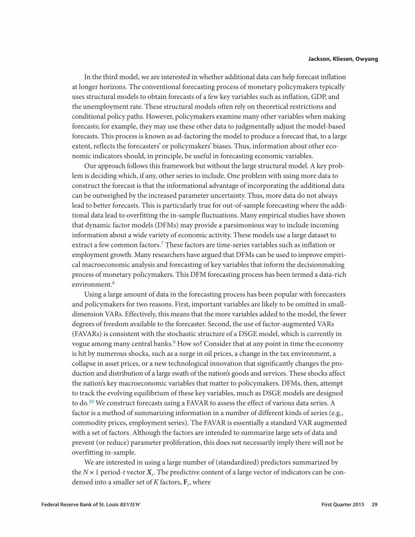
In the third model, we are interested in whether additional data can help forecast inflationat longer horizons. The conventional forecasting process of monetary policymakers typicallyuses structural models to obtain forecasts of a few key variables such as inflation, GDP, andthe unemployment rate. These structural models often rely on theoretical restrictions andconditional policy paths. However, policymakers examine many other variables when makingforecasts; for example, they may use these other data to judgmentally adjust the model-basedforecasts. This process is known as ad-factoring the model to produce a forecast that, to a largeextent, reflects the forecasters’ or policymakers’ biases. Thus, information about other eco-nomic indicators should, in principle, be useful in forecasting economic variables.

Our approach follows this framework but without the large structural model. A key prob-lem is deciding which, if any, other series to include. One problem with using more data toconstruct the forecast is that the informational advantage of incorporating the additional datacan be outweighed by the increased parameter uncertainty. Thus, more data do not alwayslead to better forecasts. This is particularly true for out-of-sample forecasting where the addi-tional data lead to overfitting the in-sample fluctuations. Many empirical studies have shownthat dynamic factor models (DFMs) may provide a parsimonious way to include incominginformation about a wide variety of economic activity. These models use a large dataset toextract a few common factors.7 These factors are time-series variables such as inflation oremployment growth. Many researchers have argued that DFMs can be used to improve empiri-cal macroeconomic analysis and forecasting of key variables that inform the decisionmakingprocess of monetary policymakers. This DFM forecasting process has been termed a data-richenvironment.8

Using a large amount of data in the forecasting process has been popular with forecastersand policymakers for two reasons. First, important variables are likely to be omitted in small-dimension VARs. Effectively, this means that the more variables added to the model, the fewerdegrees of freedom available to the forecaster. Second, the use of factor-augmented VARs(FAVARs) is consistent with the stochastic structure of a DSGE model, which is currently invogue among many central banks.9 How so? Consider that at any point in time the economyis hit by numerous shocks, such as a surge in oil prices, a change in the tax environment, acollapse in asset prices, or a new technological innovation that significantly changes the pro-duction and distribution of a large swath of the nation’s goods and services. These shocks affectthe nation’s key macroeconomic variables that matter to policymakers. DFMs, then, attemptto track the evolving equilibrium of these key variables, much as DSGE models are designedto do.10 We construct forecasts using a FAVAR to assess the effect of various data series. Afactor is a method of summarizing information in a number of different kinds of series (e.g.,commodity prices, employment series). The FAVAR is essentially a standard VAR augmentedwith a set of factors. Although the factors are intended to summarize large sets of data andprevent (or reduce) parameter proliferation, this does not necessarily imply there will not beoverfitting in-sample.

We are interested in using a large number of (standardized) predictors summarized bythe N ¥ 1 period-t vector Xt. The predictive content of a large vector of indicators can be con-densed into a smaller set of K factors, Ft, where



(3)

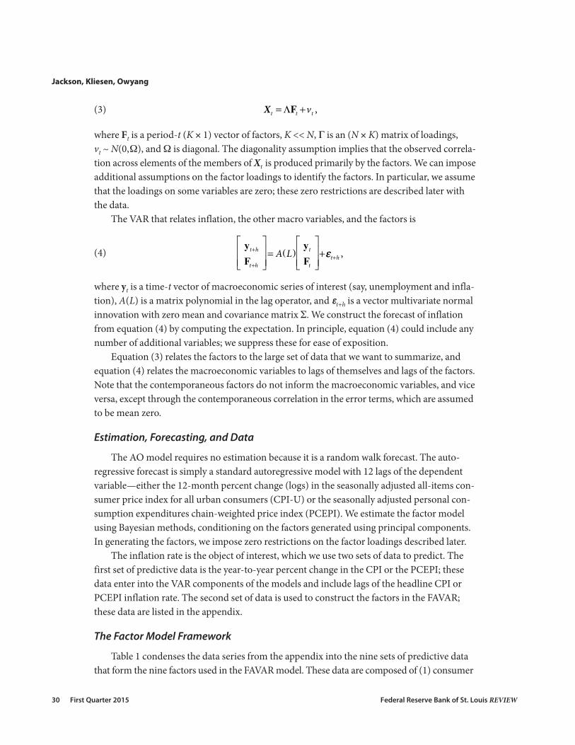
where Ft is a period-t (K ¥ 1) vector of factors, K << N, G is an (N ¥ K) matrix of loadings, vt ~ N(0,W), and W is diagonal. The diagonality assumption implies that the observed correla-tion across elements of the members of Xt is produced primarily by the factors. We can imposeadditional assumptions on the factor loadings to identify the factors. In particular, we assumethat the loadings on some variables are zero; these zero restrictions are described later withthe data.

The VAR that relates inflation, the other macro variables, and the factors is

(4)

where yt is a time-t vector of macroeconomic series of interest (say, unemployment and infla-tion), A(L) is a matrix polynomial in the lag operator, and et+h is a vector multivariate normalinnovation with zero mean and covariance matrix S. We construct the forecast of inflationfrom equation (4) by computing the expectation. In principle, equation (4) could include anynumber of additional variables; we suppress these for ease of exposition.

Equation (3) relates the factors to the large set of data that we want to summarize, andequation (4) relates the macroeconomic variables to lags of themselves and lags of the factors.Note that the contemporaneous factors do not inform the macroeconomic variables, and viceversa, except through the contemporaneous correlation in the error terms, which are assumedto be mean zero.

Estimation, Forecasting, and Data

The AO model requires no estimation because it is a random walk forecast. The auto -regressive forecast is simply a standard autoregressive model with 12 lags of the dependentvariable—either the 12-month percent change (logs) in the seasonally adjusted all-items con-sumer price index for all urban consumers (CPI-U) or the seasonally adjusted personal con-sumption expenditures chain-weighted price index (PCEPI). We estimate the factor modelusing Bayesian methods, conditioning on the factors generated using principal components.In generating the factors, we impose zero restrictions on the factor loadings described later.

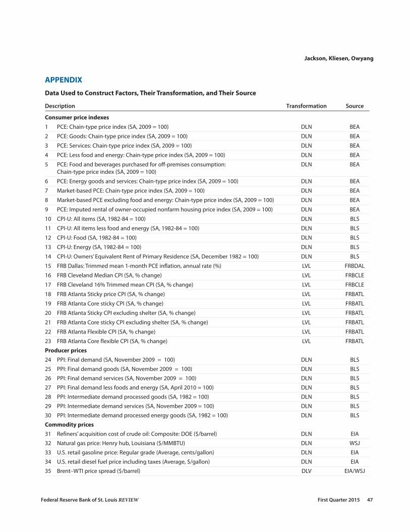
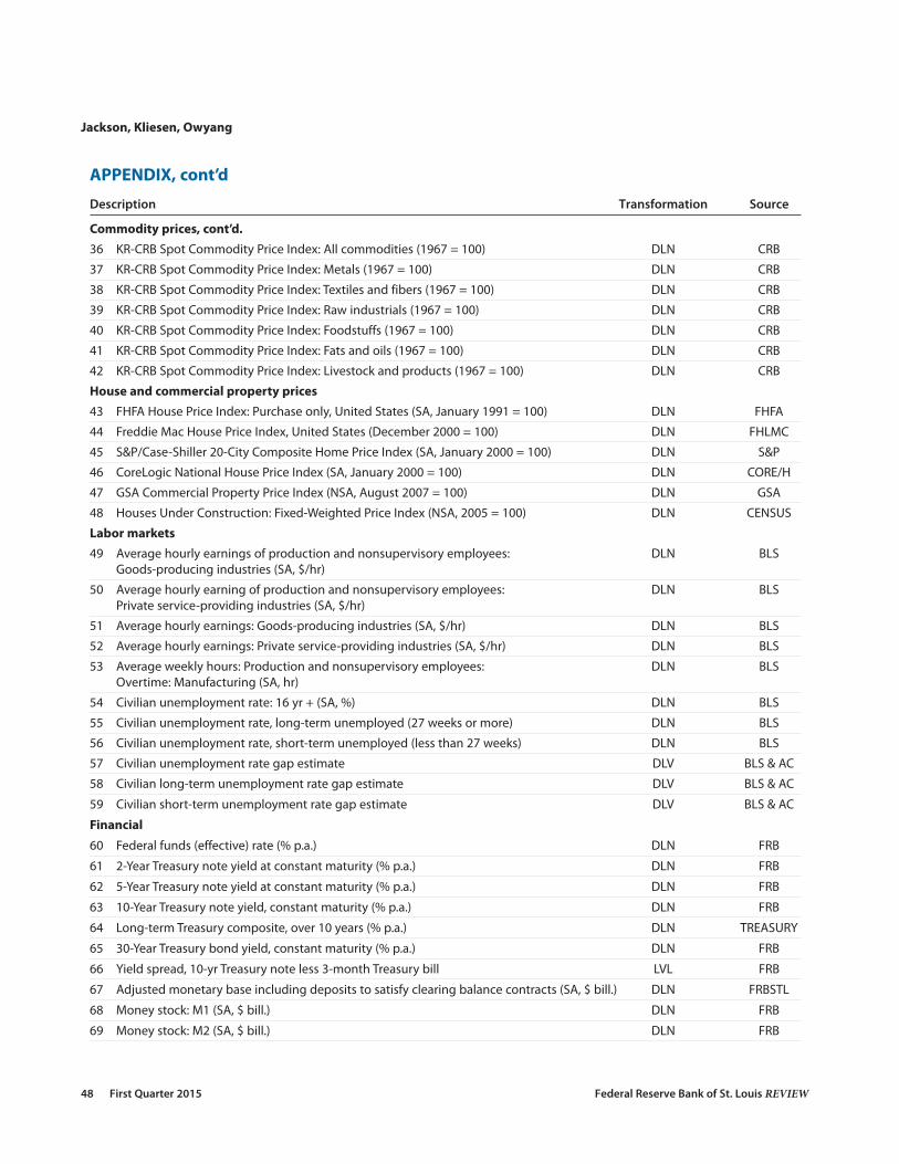
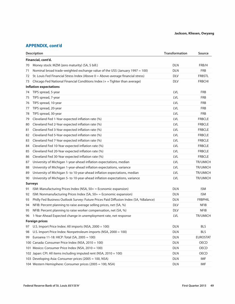
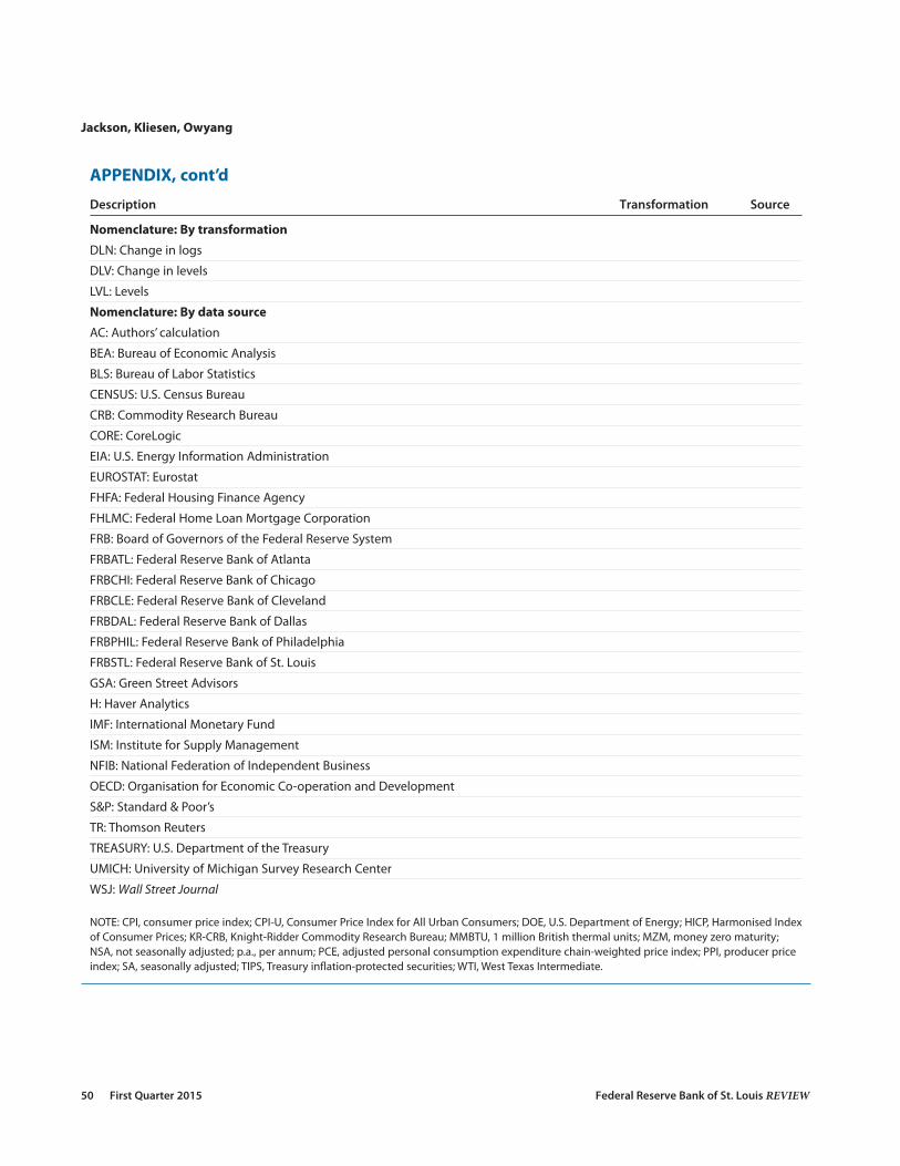
The inflation rate is the object of interest, which we use two sets of data to predict. Thefirst set of predictive data is the year-to-year percent change in the CPI or the PCEPI; thesedata enter into the VAR components of the models and include lags of the headline CPI orPCEPI inflation rate. The second set of data is used to construct the factors in the FAVAR;these data are listed in the appendix.

The Factor Model Framework

Table 1 condenses the data series from the appendix into the nine sets of predictive datathat form the nine factors used in the FAVAR model. These data are composed of (1) consumer

X vt t t= Λ +F ,

A Lt h

t h

t

tt hεε( )

=

++

++

yF

yF

,



price indexes, (2) producer price indexes, (3) commodity prices, (4) housing and commercialproperty prices, (5) labor market indicators, (6) financial variables, (7) inflation expectations,(8) survey data, and (9) foreign price variables. In choosing these variables, we wanted to focusfirst on monthly data of consumer and producer price indexes—the most obvious measure ofprice pressures. We also wanted to use series that measure prices in other dimensions, such ashouse and commercial property prices that influence rents. Similarly, we include certain com-modity prices (e.g., crude oil prices) that affect the prices of goods and services consumed byconsumers and producers.

From a broader standpoint, labor market variables have long been used by forecasters tohelp forecast inflation. According to the SPF, roughly two-thirds of survey participants incor-porate some type of Phillips curve in their forecasting model.11 As noted earlier, expectationsof financial and nonfinancial market participants (e.g., consumers and firms) underpin theNew Keynesian model. Thus, financial market expectations and surveys of consumers andbusinesses represent about a quarter of our 104 variables. Finally, Neely and Rapach (2011),Ciccarelli and Mojon (2010), and others have documented that foreign prices strongly influ-ence the U.S. domestic inflation rate. Thus, we include several foreign prices.

We estimate a single factor from each category, assuming that the factor for category i doesnot load on variables in category j, equating to zero restrictions on the loadings. This approachallows for establishing a direct interpretation of the nature of each type of factor (e.g., summa-rizing consumer prices, producer prices, and so on). The alternative approach would be toextract a set of factors from the entire set of predictive variables. However, this makes it diffi-cult to obtain a clear, definitive interpretation of which factor represents which source of infla-tionary pressures. We estimate the factors over two sample periods: February 1964–December2013 and January 1983–December 2013. The latter period is sometimes referred to as the GreatModeration, which refers to the fact that the volatility of output, inflation, and many other



Table 1

Types of Data Used in Factor Estimation

Description No. of individual series

1. Consumer price indexes 23

2. Producer price indexes 7

3. Commodity prices 12

4. House and commercial property prices 6

5. Labor markets 11

6. Financial 14

7. Inflation expectations 17

8. Business and consumer surveys 6

9. Foreign prices 8

Total No. of series 104

NOTE: See the appendix for individual series, data transformations, and sources.

macroeconomic time-series variables was much larger before 1983 than after 1983.12 We usea method for generating the principal components with unbalanced panels to estimate thefactors. That is, the date of the first observation for all series is not the same; we then generatea separate factor for each subgroup determined earlier. This process yields an unbalanced panelof factors. Most factors begin in January 1964; the exception is the factor constructed usinginflation expectations measures, the earliest of which (University of Michigan surveys of con-sumers) begins in January 1978. Finally, we perform two experiments. In the first experiment,we conduct out-of-sample forecast experiments using monthly revised data from the February1964–December 2013 period. Here, we include eight different factors, excluding those relatedto inflation expectations. In the second experiment, we repeat the out-of-sample forecastswith data from the January 1983–December 2013 period and use a set of nine factors, nowincluding the inflation expectations factor.

Factor Loadings

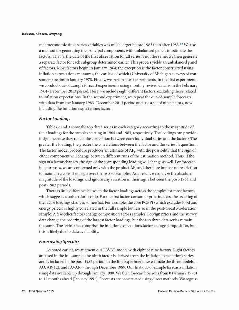
Tables 2 and 3 show the top three series in each category according to the magnitude oftheir loadings for the samples starting in 1964 and 1983, respectively. The loadings can provideinsight because they reflect the correlation between each individual series and the factors: Thegreater the loading, the greater the correlations between the factor and the series in question.The factor model procedure produces an estimate of L̂Ft, with the possibility that the sign ofeither component will change between different runs of the estimation method. Thus, if thesign of a factor changes, the sign of the corresponding loading will change as well. For forecast-ing purposes, we are concerned only with the product L̂Ft and therefore impose no restrictionto maintain a consistent sign over the two subsamples. As a result, we analyze the absolutemagnitude of the loadings and ignore any variation in their signs between the post-1964 andpost-1983 periods.

There is little difference between the factor loadings across the samples for most factors,which suggests a stable relationship. For the first factor, consumer price indexes, the ordering ofthe factor loadings changes somewhat. For example, the core PCEPI (which excludes food andenergy prices) is highly correlated in the full sample but less so in the post-Great Moderationsample. A few other factors change composition across samples. Foreign prices and the surveydata change the ordering of the largest factor loadings, but the top three data series remainthe same. The series that comprise the inflation expectations factor change composition, butthis is likely due to data availability.

Forecasting Specifics

As noted earlier, we augment our FAVAR model with eight or nine factors. Eight factorsare used in the full sample; the ninth factor is derived from the inflation expectations seriesand is included in the post-1983 period. In the first experiment, we estimate the three models—AO, AR(12), and FAVAR—through December 1989. Our first out-of-sample forecasts inflationusing data available up through January 1990. We then forecast horizons from 0 (January 1990)to 12 months ahead (January 1991). Forecasts are constructed using direct methods: We regress





Table 2

Three Largest Factor Loadings Within Each Category: Full Post-February 1964 Sample

Consumer price indexes

FRB Cleveland: Median CPI, 1-month percent change –1.21

FRB Atlanta: Sticky CPI, 1-month percent change 1.18

PCE chain-type price index, market-based excluding food and energy –1.18

Producer prices

PPI: Final demand 1.02

PPI: Final demand goods 1.01

PPI: Final demand excluding food and energy 1.01

Commodity prices

KR-CRB Spot Commodity Price Index: All Commodities 1.38

CRB Spot Raw Industrials Price Index 1.22

U.S. retail gasoline price: Regular grade 1.20

House and commercial property prices

Case-Shiller Composite 20-City House Price Index 1.01

FHFA House Price Index, Purchase Only 1.01

CoreLogic National House Price Index (SA, Jan. 2000 = 100) 1.00

Labor markets

Civilian unemployment rate 1.37

Civilian unemployment rate gap estimate 1.37

Average hourly earnings: Private goods-producing, all employees 1.36

Financial

10-Year Treasury yield, constant maturity 1.61



Inflation expectations

TIPS spread, 5-year 1.001



Surveys

ISM: Nonmanufacturing Prices Paid index –1.28

NFIB: Percent of firms planning to raise average selling prices, net –1.17

ISM: Manufacturing Prices Paid index –1.07

Foreign prices

Euro area harmonized overall CPI 1.17

U.S. Import Price Index, All Imports 1.15

U.S. Import Price Index, Nonpetroleum Imports 1.15

NOTE: CRB, Commodity Research Bureau; FHFA, Federal Housing Finance Agency; ISM, Institute for Supply Management;NFIB, National Federation of Independent Business; PPI, producer price index; SA, seasonally adjusted; TIPS, Treasuryinflation-protected securities.

SOURCE: Authors’ calculations.



Table 3

Three Largest Factor Loadings Within Each Category: Full Post-January 1983 Sample


FRB Cleveland: 16% Trimmed mean CPI, 1-month percent change 1.35

FRB Dallas: Trimmed mean, 1-month PCE inflation rate 1.34

FRB Atlanta: Sticky CPI, 1-month percent change 1.32

Producer prices

PPI: Final demand 1.02

PPI: Final demand goods 1.01

PPI: Final demand excluding food and energy 1.01

Commodity prices

KR-CRB Spot Commodity Price Index: All Commodities 1.42

CRB Spot Raw Industrials Price Index 1.30

CRB Spot Livestock and Products Price Index 1.12

House and commercial property prices

Case-Shiller Composite 20-City House Price Index 1.23

CoreLogic National House Price Index (SA, Jan. 2000 = 100) 1.18

FHFA House Price Index: Purchase Only 1.07

Labor markets

Civilian unemployment rate 1.46

Civilian unemployment rate gap estimate 1.43

Average hourly earnings: Private goods-producing, all employees 1.29

Financial

10-Year Treasury yield, constant maturity –1.60

5-Year Treasury yield, constant maturity –1.58

Yield on Treasury long-term composite bond –1.53



FRB Cleveland, 5-Year expected inflation rate –1.10

FRB Cleveland, 7-Year expected Inflation rate –1.10

Surveys

ISM: Nonmanufacturing Prices Paid Index –1.40

ISM: Manufacturing Prices Paid Index –1.26

NFIB: Percent of firms planning to raise average selling prices, net –1.22

Foreign prices

U.S. Import Price Index, All Imports –1.41

Euro area harmonized overall CPI –1.42

U.S. Import Price Index: Nonpetroleum Commodities –1.34

NOTE: CRB, Commodity Research Bureau; FHFA, Federal Housing Finance Agency; ISM, Institute for Supply Management;NFIB, National Federation of Independent Business; PPI, producer price index; SA, seasonally adjusted; TIPS, Treasuryinflation-protected securities.


directly the forward data on the available information. We use a recursive estimation schemeso that all past information is incorporated into the model estimates. We have three FAVARmodels: 1 lag, 6 lags, and 12 lags. Because estimation of the FAVAR is computationally inten-sive, we reestimate the model only once per year in January, when we assume all data from theprevious year are available. The forecasts are constructed monthly, which means the principalcomponents are updated monthly, but the forecasts are constructed using that year’s estimateof the model parameters.

Results

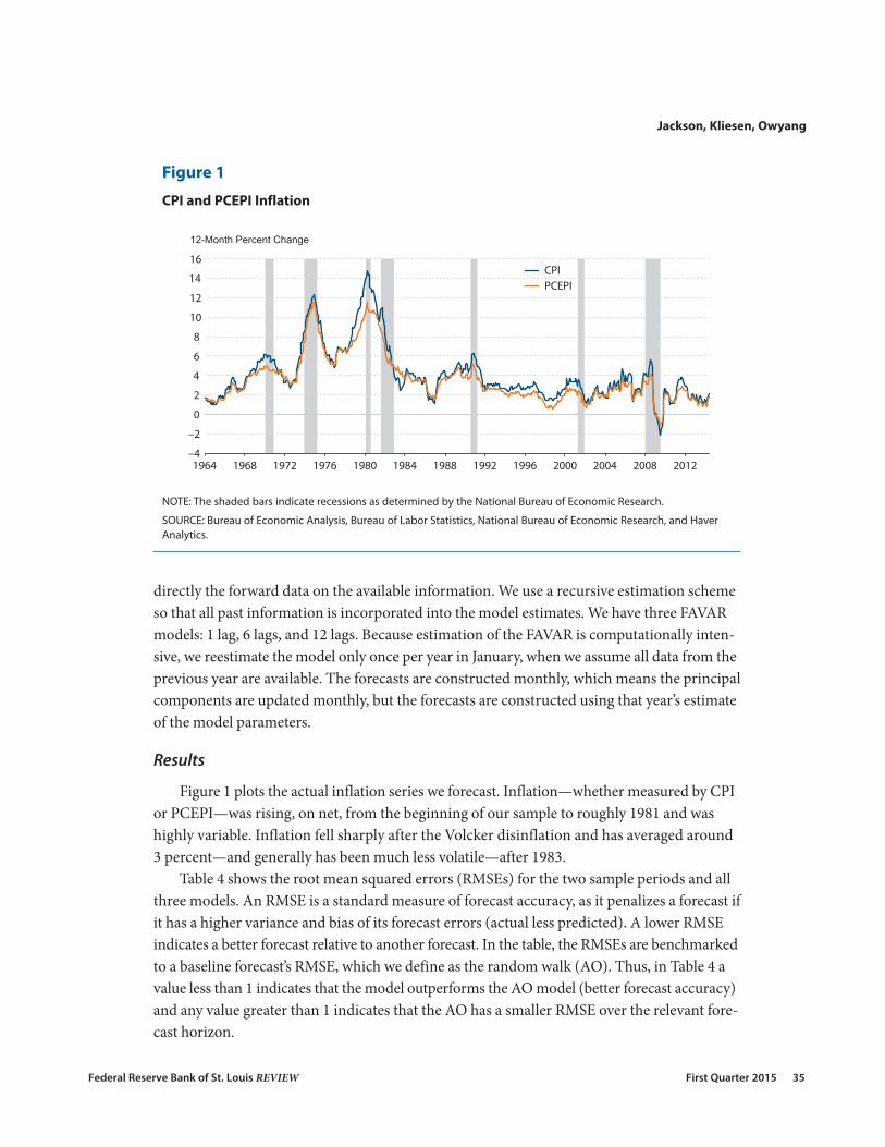
Figure 1 plots the actual inflation series we forecast. Inflation—whether measured by CPIor PCEPI—was rising, on net, from the beginning of our sample to roughly 1981 and washighly variable. Inflation fell sharply after the Volcker disinflation and has averaged around3 percent—and generally has been much less volatile—after 1983.

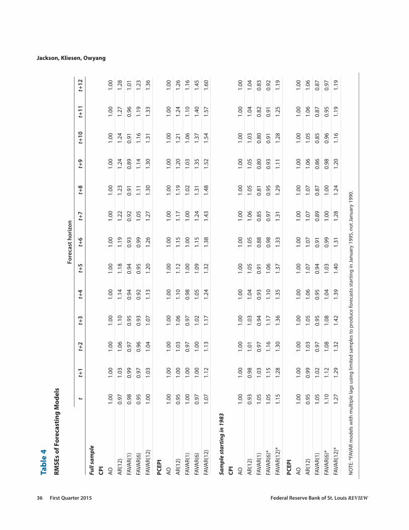
Table 4 shows the root mean squared errors (RMSEs) for the two sample periods and allthree models. An RMSE is a standard measure of forecast accuracy, as it penalizes a forecast ifit has a higher variance and bias of its forecast errors (actual less predicted). A lower RMSEindicates a better forecast relative to another forecast. In the table, the RMSEs are benchmarkedto a baseline forecast’s RMSE, which we define as the random walk (AO). Thus, in Table 4 avalue less than 1 indicates that the model outperforms the AO model (better forecast accuracy)and any value greater than 1 indicates that the AO has a smaller RMSE over the relevant fore-cast horizon.



–4

–2

0

2

4

6

8

10

12

14

16

1964 1968 1972 1976 1980 1984 1988 1992 1996 2000 2004 2008 2012

CPI PCEPI

12-Month Percent Change

Figure 1

CPI and PCEPI Inflation

NOTE: The shaded bars indicate recessions as determined by the National Bureau of Economic Research.

SOURCE: Bureau of Economic Analysis, Bureau of Labor Statistics, National Bureau of Economic Research, and HaverAnalytics.



Tabl

e 4

RMSE

s of

For

ecas

ting

Mod

els

Fore

cast

hor

izon

tt+

1t+

2t+

3t+

4t+

5t+

6t+

7t+

8t+

9t+

10t+

11t+

12

Full

sam

ple

CPI

AO1.

001.

001.

001.

001.

001.

001.

001.

001.

001.

001.

001.

001.

00

AR(

12)

0.97

1.03

1.06

1.10

1.14

1.18

1.19

1.22

1.23

1.24

1.24

1.27

1.28

FAVA

R(1)

0.98

0.99

0.97

0.95

0.94

0.94

0.93

0.92

0.91

0.89

0.91

0.96

1.01

FAVA

R(6)

0.95

0.97

0.96

0.93

0.92

0.95

0.99

1.05

1.11

1.14

1.16

1.19

1.23

FAVA

R(12

)1.

001.

031.

041.

071.

131.

201.

261.

271.

301.

301.

311.

331.

36

PCEP

I

AO1.

001.

001.

001.

001.

001.

001.

001.

001.

001.

001.

001.

001.

00

AR(

12)

0.95

1.00

1.03

1.06

1.10

1.12

1.15

1.17

1.19

1.20

1.21

1.24

1.26

FAVA

R(1)

1.00

1.00

0.97

0.97

0.98

1.00

1.00

1.00

1.02

1.03

1.06

1.10

1.16

FAVA

R(6)

0.97

1.00

1.00

1.02

1.05

1.09

1.15

1.24

1.31

1.35

1.37

1.40

1.45

FAVA

R(12

)1.

071.

121.

131.

171.

241.

321.

381.

431.

481.

521.

541.

571.

60

Sam

ple

star

ting

in 1

983

CPI

AO1.

001.

001.

001.

001.

001.

001.

001.

001.

001.

001.

001.

001.

00

AR(

12)

0.93

0.98

1.01

1.03

1.04

1.05

1.05

1.06

1.05

1.05

1.03

1.04

1.04

FAVA

R(1)

1.05

1.03

0.97

0.94

0.93

0.91

0.88

0.85

0.81

0.80

0.80

0.82

0.83

FAVA

R(6)

*1.

051.

151.

161.

171.

101.

060.

980.

970.

950.

930.

910.

910.

92

FAVA

R(12

)*1.

151.

281.

301.

361.

351.

371.

331.

311.

291.

111.

281.

251.

19

PCEP

I

AO1.

001.

001.

001.

001.

001.

001.

001.

001.

001.

001.

001.

001.

00

AR(

12)

0.95

0.99

1.03

1.05

1.06

1.07

1.07

1.07

1.07

1.06

1.05

1.06

1.06

FAVA

R(1)

1.05

1.02

0.97

0.95

0.95

0.94

0.91

0.89

0.87

0.86

0.85

0.87

0.87

FAVA

R(6)

*1.

101.

121.

081.

081.

041.

030.

991.

001.

000.

980.

960.

950.

97

FAVA

R(12

)*1.

271.

291.

321.

421.

391.

401.

311.

281.

241.

201.

161.

191.

19

NO

TE: *

FAVA

R m

odel

s w

ith m

ultip

le la

gs u

sing

lim

ited

sam

ples

to p

rodu

ce fo

reca

sts

star

ting

in J

anua

ry 1

995,

not

Jan

uary

199

0.

We now consider some key findings from the full sample. First, the AO model performsreasonably well across most horizons. The AO model clearly outperforms the AR(12) model—except for the contemporaneous period (t = 0)—for both measures of inflation.

In the full sample, the FAVAR(1) model is generally more accurate in forecasting CPIinflation than the AO model for times t to t + 11. The FAVAR(6) model performs much betterthrough the first half of the forecast horizon (up through 6 months). The forecasting accuracyof the FAVAR(12) model is worse than the FAVAR(1) and FAVAR(6) models across all horizons.The longer the forecast horizon, the worse the FAVAR(12) model performs—indeed, worsethan the AR(12) model. In the full sample, the FAVAR models generally do not forecast PCEinflation as well as the AO model. The random walk model tends to dominate all other modelsfor forecasting PCE inflation in the full sample.

Table 4 also shows the forecasting performance in the post-1983 sample. In this experi-ment, the model is estimated with data from January 1983 through December 1994 and thenout-of-sample forecasting begins in January 1995. In this experiment, we add the inflationexpectations factor (for a total of nine factors). As before, the models are then reestimated ayear later and out-of-sample forecasts are produced. Table 4 clearly indicates that adding theinflation expectations factor to the FAVAR model produces markedly smaller RMSEs for bothinflation measures than either the AO or AR(12) models. Indeed, at 6 and 12 months ahead,the FAVAR(1) forecast for CPI inflation produces RMSEs that are 12 percent and 17 percentsmaller, respectively, than the AO model. The RMSEs are a bit larger for the 6-lag FAVAR. ForPCEPI inflation, the RMSEs are a bit larger than for CPI inflation, but again the FAVAR(1) andFAVAR(6) models perform measurably better than the AO or AR(12) models. The FAVAR(12)model has a much higher RMSE for both CPI and PCEPI inflation than the other modelsacross all horizons.

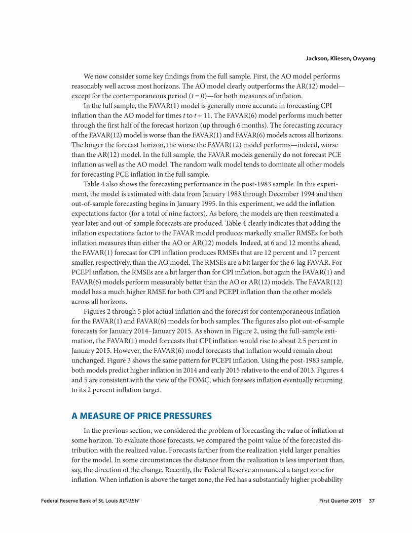
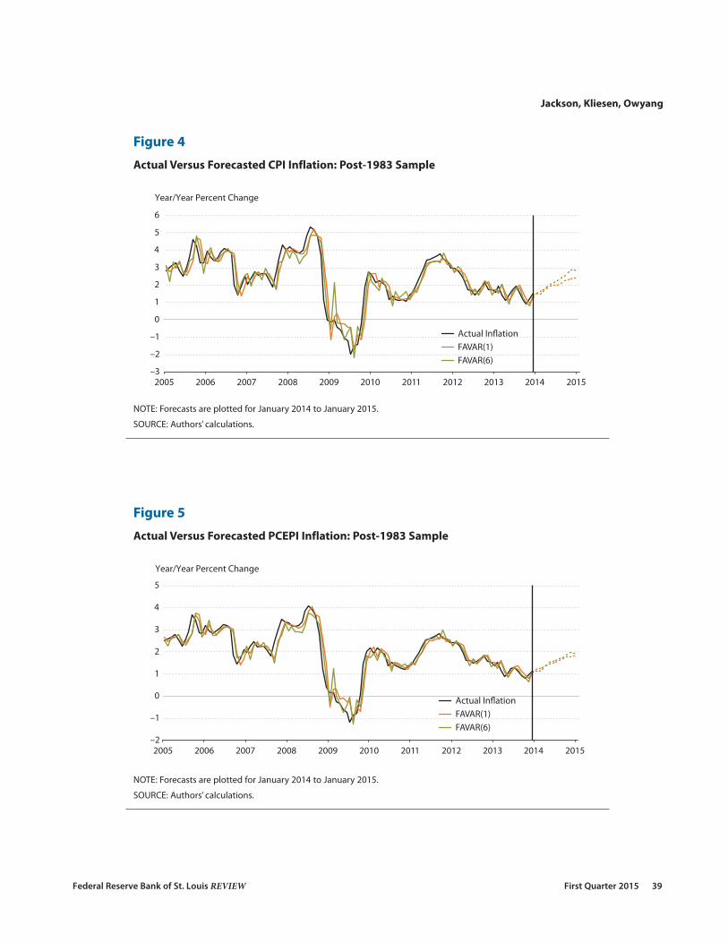
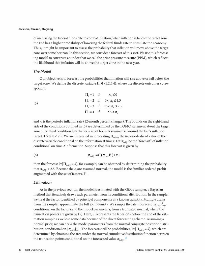
Figures 2 through 5 plot actual inflation and the forecast for contemporaneous inflationfor the FAVAR(1) and FAVAR(6) models for both samples. The figures also plot out-of-sampleforecasts for January 2014–January 2015. As shown in Figure 2, using the full-sample esti-mation, the FAVAR(1) model forecasts that CPI inflation would rise to about 2.5 percent inJanuary 2015. However, the FAVAR(6) model forecasts that inflation would remain aboutunchanged. Figure 3 shows the same pattern for PCEPI inflation. Using the post-1983 sample,both models predict higher inflation in 2014 and early 2015 relative to the end of 2013. Figures 4and 5 are consistent with the view of the FOMC, which foresees inflation eventually returningto its 2 percent inflation target.

A MEASURE OF PRICE PRESSURESIn the previous section, we considered the problem of forecasting the value of inflation at

some horizon. To evaluate those forecasts, we compared the point value of the forecasted dis-tribution with the realized value. Forecasts farther from the realization yield larger penaltiesfor the model. In some circumstances the distance from the realization is less important than,say, the direction of the change. Recently, the Federal Reserve announced a target zone forinflation. When inflation is above the target zone, the Fed has a substantially higher probability





–3

–2

–1

0

1

2

3

4

5

6

2005 2006 2007 2008 2009 2010 2011 2012 2013 2014 2015

Actual In!ation FAVAR(1) FAVAR(6)

Year/Year Percent Change

Figure 2

Actual Versus Forecasted CPI Inflation: Full Sample

NOTE: Forecasts are plotted for January 2014 to January 2015.


–2

–1

0

1

2

3

4

5

2005 2006 2007 2008 2009 2010 2011 2012 2013 2014 2015



Figure 3

Actual Versus Forecasted PCEPI Inflation: Full Sample





–3

–2

–1

0

1

2

3

4

5

6

2005 2006 2007 2008 2009 2010 2011 2012 2013 2014 2015



Figure 4

Actual Versus Forecasted CPI Inflation: Post-1983 Sample



–2

–1

0

1

2

3

4

5

2005 2006 2007 2008 2009 2010 2011 2012 2013 2014 2015



Figure 5

Actual Versus Forecasted PCEPI Inflation: Post-1983 Sample



of increasing the federal funds rate to combat inflation; when inflation is below the target zone,the Fed has a higher probability of lowering the federal funds rate to stimulate the economy.Thus, it might be important to assess the probability that inflation will move above the targetzone over some horizon. In this section, we consider a forecast of this sort. We use this forecast-ing model to construct an index that we call the price pressure measure (PPM), which reflectsthe likelihood that inflation will be above the target zone in the next year.

The Model

Our objective is to forecast the probabilities that inflation will rise above or fall below thetarget zone. We define the discrete variable Pt ∈ {1,2,3,4}, where the discrete outcomes corre-spond to

(5)

and pt is the period-t inflation rate (12-month percent changes). The bounds on the right-handside of the conditions outlined in (5) are determined by the FOMC statement about the targetzone. The third condition establishes a set of bounds symmetric around the Fed’s inflationtarget: 1.5 ≤ pt < 2.5. We are interested in forecasting Pt+h|t, the h-period-ahead value of thediscrete variable conditional on the information at time t. Let pt+h|t be the “forecast” of inflationconditional on time-t information. Suppose that this forecast is given by

(6)

then the forecast Pr[Pt+h|t = k], for example, can be obtained by determining the probabilitythat pt+h|t > 2.5. Because the et are assumed normal, the model is the familiar ordered probitaugmented with the set of factors, Ft.

Estimation

As in the previous section, the model is estimated with the Gibbs sampler, a Bayesianmethod that iteratively draws each parameter from its conditional distribution. In the sampler,we treat the factor identified by principal components as a known quantity. Multiple drawsfrom the sampler approximate the full joint density. We sample the latent forecast {pt+h|t}

Tt=1,

conditional on the factors and the model parameters, from a truncated normal, where thetruncation points are given by (5). Here, T represents the h periods before the end of the esti-mation sample as we lose some data because of the direct forecasting scheme. Assuming anormal prior, we can draw the model parameters from the normal conjugate posterior distri-bution, conditional on {pt+h|t}

Tt=1. The forecasts will be probabilities, Pr[Pt+h|t = k], which are

determined by obtaining the area under the normal cumulative distribution function betweenthe truncation points conditional on the forecasted value pt+h|t.13

.. .

.

t t

t t

t t

t t

πππ

π

Π = ≤Π = < ≤Π = < ≤Π = <

1 if 02 if 0 1 53 if 1 5 2 54 if 2 5

Gt h|t t t tπ π ε( )= ++ − F, ;1



Forming the Index

The objective of forming the PPM is to assess the likelihood that inflation will rise abovethe target. We computed {Pr[pt+h|t > 2.5]}12

h=0 using the ordered probit model. We can computea weighted sum of these probabilities to form our PPM:

where wh is the weight placed on horizon h and Shwh = 1. The nature of the weights dependson whether longer or shorter horizon forecasts are more valued. In this case, we opt for equalweighting.

Results

Our PPM measures the probability that the expected inflation rate (12-month percentchanges) over the next 12 months—the forecast horizon—will exceed 2.5 percent. This bin(2.5 percent) exceeds the Fed’s 2 percent inflation target. We calculate our PPMs from thesetwo modes. These PPMs are plotted in Figure 6 for CPI and PCEPI inflation using the 1- and6-lag ordered probit models.14 We plot the smoothed series, which is a six-month movingaverage. Figure 6 shows that, over most of this sample period (January 1990–January 2014),the PPM for CPI inflation was greater than 0.5. By contrast, the probabilities for PCEPI infla-tion exceeded 0.5 by an appreciably smaller percentage over the sample period. Since the endof the recent recession, the PPMs have been significantly below 0.5 for PCEPI inflation butmoderately less so for CPI inflation. In one sense, the models are picking up the fact that infla-tion was higher before the recession and that CPI inflation is generally higher on average thanPCEPI inflation. For the January 1990–December 2007 period, CPI inflation averaged 2.9 per-cent and PCEPI inflation averaged 2.3 percent. However, since January 2008, CPI inflationhas averaged 2 percent and PCEPI inflation has averaged 1.7 percent.

At any point in time, the PPMs plotted in Figure 6 are unweighted averages of the proba-bility that the forecasted inflation rate will average more than 2.5 percent over the next 12months. However, policymakers know that a standard error around the point estimate isassociated with any forecast. For example, the Bank of England’s fan charts contain both pointestimates and error bands around these point estimates that can be thought of as probabilities.In the simplest terms, if monetary policymakers project that inflation over the following yearwill be 2 percent, there is some probability that inflation will be less than 2 percent and someprobability that inflation will be more than 2 percent.

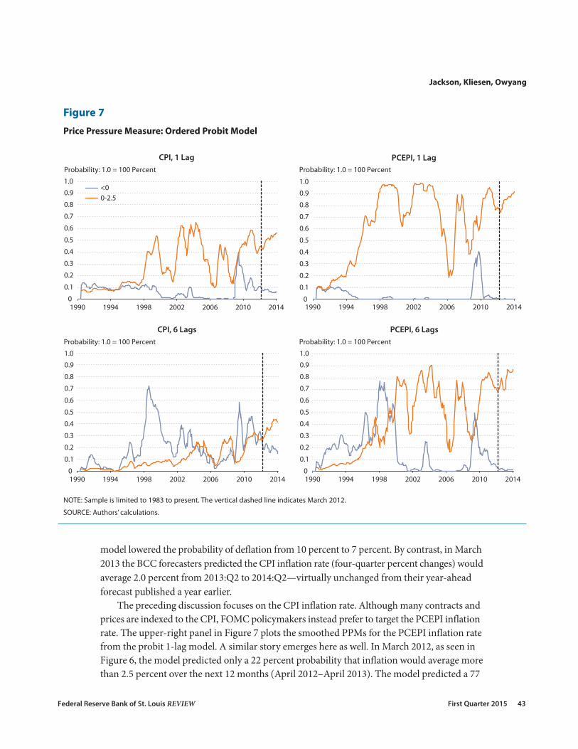
The ordered probit model estimated earlier provides probabilities that inflation willexceed 2.5 percent, on average, over the next 12 months. But our model also allows us toassess the probability that inflation will average something different. In this case, we structurethe model to assess the probability that inflation will fall within one of four bins: less thanzero (deflation); 0 percent to 1.5 percent; 1.5 percent to 2.5 percent; and more than 2.5 per-cent. The last bin is our PPM plotted in Figure 6; Figure 7 plots the other three probabilities.For ease of discussion, we condense the second and third bins into one, leaving two sets of

PPM w . ,h h t h|tπ= Σ > = +Pr 2 5

0

12



probabilities: Inflation will be less than zero (deflation) over the next 12 months and inflationwill average between 0 percent and 2.5 percent.

In March 2012, policymakers observed that the CPI had increased by 2.3 percent overthe previous year (March 2011–March 2012). The outlook of professional forecasters, asjudged by the Blue Chip Consensus (BCC), was that the CPI inflation rate (four-quarter per-cent changes) would average 2.1 percent from 2012:Q2 to 2013:Q2. However, as noted earlier,policymakers generally eschew point estimates in favor of probabilities.15 In this case, as shownin Figure 7, it is the probability that inflation will be above or below the forecast consensus.

In March 2012, the model predicted a 45 percent probability that CPI inflation wouldaverage more than 2.5 percent from April 2012 to April 2013 (see Figure 6). This relativelyhigh probability could have reflected the fact that crude oil prices rose by 24 percent fromSeptember 2011 to March 2012. However, the model also predicted an equal probability thatinflation would average between 0 percent and 2.5 percent, with only a 10 percent probabilitythat inflation would average less than zero over the next 12 months. (This date is noted by thevertical dashed line in the figure.)16 But forecasters and policymakers were instead surprisedbecause inflation fell from 2.3 percent in April 2012 to 1.1 percent in April 2013. The modelperformed reasonably well if one takes into account the probability of deflation: There was agreater than 50 percent probability that inflation would be less than 2.5 percent.

A year later, in March 2013, the model lowered the probability that inflation would averagemore than 2.5 percent over the next year (April 2013–April 2014) from 45 percent to 43 per-cent (see Figure 6). However, the model raised the probability that inflation would be between0 percent and 2.5 percent over the following year from 45 percent to 50 percent. Likewise, the



0

0.1

0.2

0.3

0.4

0.5

0.6

0.7

0.8

0.9

1.0

1990 1994 1998 2002 2006 2010 2014

1 Lag 6 Lags

Probability: 1.0 = 100 Percent

1990 1994 1998 2002 2006 2010 2014

Probability: 1.0 = 100 Percent

0

0.1

0.2

0.3

0.4

0.5

0.6

0.7

0.8

0.9

1.0

1 Lag 6 Lags

CPI PCEPI

Figure 6

Price Pressure Measure: Probability That Inflation Exceeds 2.5 Percent

NOTE: Sample is limited to 1983 to present. The vertical dashed line indicates March 2012.


model lowered the probability of deflation from 10 percent to 7 percent. By contrast, in March2013 the BCC forecasters predicted the CPI inflation rate (four-quarter percent changes) wouldaverage 2.0 percent from 2013:Q2 to 2014:Q2—virtually unchanged from their year-aheadforecast published a year earlier.

The preceding discussion focuses on the CPI inflation rate. Although many contracts andprices are indexed to the CPI, FOMC policymakers instead prefer to target the PCEPI inflationrate. The upper-right panel in Figure 7 plots the smoothed PPMs for the PCEPI inflation ratefrom the probit 1-lag model. A similar story emerges here as well. In March 2012, as seen inFigure 6, the model predicted only a 22 percent probability that inflation would average morethan 2.5 percent over the next 12 months (April 2012–April 2013). The model predicted a 77



0

0.1

0.2

0.3

0.4

0.5

0.6

0.7

0.8

0.9

1.0

1990 1994 1998 2002 2006 2010 2014

CPI, 1 Lag

1990 1994 1998 2002 2006 2010 2014

1990 1994 1998 2002 2006 2010 2014 1990 1994 1998 2002 2006 2010 2014

0

0.1

0.2

0.3

0.4

0.5

0.6

0.7

0.8

0.9

1.0

PCEPI, 1 Lag

0

0.1

0.2

0.3

0.4

0.5

0.6

0.7

0.8

0.9

1.0

CPI, 6 Lags

0

0.1

0.2

0.3

0.4

0.5

0.6

0.7

0.8

0.9

1.0

PCEPI, 6 Lags

<00-2.5

Probability: 1.0 = 100 Percent Probability: 1.0 = 100 Percent

Probability: 1.0 = 100 Percent Probability: 1.0 = 100 Percent

Figure 7

Price Pressure Measure: Ordered Probit Model

NOTE: Sample is limited to 1983 to present. The vertical dashed line indicates March 2012.


percent probability that inflation would average between 0 and 2.5 percent. The probability thatinflation would average less than zero (deflation) was less than 1 percent. Although the BCCdoes not forecast the PCEPI inflation rate, forecasts for the FOMC’s preferred inflation measureare reported in the Philadelphia Fed’s SPF. In its February 2012 report, the SPF predicted thePCEPI would increase from 1.7 percent (quarterly rate, annualized) in 2012:Q1 to 2 percentin 2013:Q1. Mirroring the dip in the CPI inflation rate, the PCEPI inflation rate unexpect-edly slowed from 2 percent in April 2012 to 1 percent in April 2013.17 In this case, the modelperformed well, perceiving a relatively high probability that inflation would remain below 2.5 percent.

The unexpected slowing in inflation, perhaps not surprisingly, affected the probabilitydistributions a year later, in March 2013. By then, the model estimated the probability thatPCEPI inflation would average between 0 and 2.5 percent over the next 12 months (April2013–April 2014) had increased from 77 percent to 85 percent. The probability of deflationwas lowered from 0.8 percent to 0.3 percent. As shown in Figure 6, the probability that inflationwould average more than 2.5 percent declined from 22 percent to 14 percent. Despite thismarked shift in the probability distribution, in mid-February 2013 the SPF was still projectingthat PCEPI inflation would increase to 2 percent in 2014:Q1. Once again, the actual data aremore consistent with our model: From April 2013 to March 2014 (the latest available data),the 12-month change in the PCEPI inflation rate increased from 1 percent to 1.2 percent. Thetwo lower charts in Figure 7 show the PPMs using the 6-lag probit for the post-1983 sample.They show trends broadly similar to the 1-lag model.

Out-of-Sample PCEPI Inflation Forecasts

Table 4 indicates that the best model for forecasting inflation one year ahead is theFAVAR(1) for CPI inflation estimated using the post-1983 sample. Although the FAVAR(1)RMSEs for PCEPI inflation are slightly larger, this section nonetheless focuses on this measurebecause the FOMC targets the PCEPI inflation rate. Recall that Figure 5 plots the PCEPI infla-tion forecasts for January 2014–January 2015. For purposes of comparison, FOMC participantsin December 2013 projected that the PCEPI inflation rate would increase by 1.5 percent in2014 (2013:Q4–2014:Q4).18 Thus, our preferred inflation forecasting model expected inflationto rise by slightly more than the FOMC’s projection, from 1 percent in December 2013 to 1.8percent in December 2014 and in January 2015.19

Figure 8 shows the probability distribution of this out-of-sample forecast from January2014 to January 2015. The upper-left panel indicates that the model predicts a very small—roughly zero—probability of deflation over this horizon. For this forecast, we can separate the0 percent to 2.5 percent probability distribution into two bins: 0 to 1.5 percent (upper-rightpanel) and 1.5 percent to 2.5 percent (lower-left panel). In the upper-right panel, the modelpredicts a more than 50 percent probability that PCEPI inflation would remain in the 0 to 1.5percent range through the first five months of 2014. Thereafter, the model predicts a higherprobability—averaging slightly less than 50 percent—that PCEPI inflation would rise to morethan 1.5 percent but remain below 2.5 percent. The lower-right panel shows an increasingprobability—over the second half of 2014—that inflation would increase by more than 2.5percent by the end of the forecast horizon.



CONCLUSIONThe FOMC, like most major central banks, devotes significant resources to forecasting

key economic variables such as real GDP growth, employment, and inflation. The outlook forthese variables also matters a great deal to businesses and financial market participants. Forexample, when decisions are made to expend scarce resources or price financial assets, suchdecisions—which must be made in the present—are based on expectations of future economicconditions. In this article, we present a factor-augmented Bayesian vector autoregressive fore-casting model that significantly outperforms both a benchmark random walk model and a puretime-series model. The empirical literature has shown that random walk models tend to beamong the most accurate across a variety of simple time-series model specifications. A key



0 0.1 0.2 0.3 0.4 0.5 0.6 0.7 0.8 0.9 1.0

Jan. 2

014

Feb. 2014

Mar. 2014

Apr. 2014

May 2014

Jun. 2

014

Jul. 2

014

Aug. 2014

Sep. 2014

Oct. 2014

Nov. 2014

Dec. 2014

Jan. 2

015

Probability That PCEPI In�ation Will Be Negative (Jan. 2014–Jan. 2015)

0 0.1 0.2 0.3 0.4 0.5 0.6 0.7 0.8 0.9 1.0

0 0.1 0.2 0.3 0.4 0.5 0.6 0.7 0.8 0.9 1.0

0 0.1 0.2 0.3 0.4 0.5 0.6 0.7 0.8 0.9 1.0

Probability That PCEPI In�ation Will Be 0% to 1.5% (Jan. 2014–Jan. 2015)

Probability That PCEPI In�ation Will Be Above 2.5% (Jan. 2014–Jan. 2015)Probability That PCEPI In�ation Will Be 1.5% to 2.5% (Jan. 2014–Jan. 2015)

Probability: 1.0 = 100% Probability: 1.0 = 100%

Probability: 1.0 = 100%Probability: 1.0 = 100%

Jan. 2

014

Feb. 2014

Mar. 2014

Apr. 2014

May 2014

Jun. 2

014

Jul. 2

014

Aug. 2014

Sep. 2014

Oct. 2014

Nov. 2014

Dec. 2014

Jan. 2

015

Jan. 2

014

Feb. 2014

Mar. 2014

Apr. 2014

May 2014

Jun. 2

014

Jul. 2

014

Aug. 2014

Sep. 2014

Oct. 2014

Nov. 2014

Dec. 2014

Jan. 2

015

Jan. 2

014

Feb. 2014

Mar. 2014

Apr. 2014

May 2014

Jun. 2

014

Jul. 2

014

Aug. 2014

Sep. 2014

Oct. 2014

Nov. 2014

Dec. 2014

Jan. 2

015

Figure 8

PCEPI Inflation Probabilities


innovation in our article is the use of nine factors in an ordered probit model to assess theprobability distribution of the model’s point forecasts. We term these probabilities a pricepressure measure. Our measure shows a relatively high probability that inflation in 2014would be higher than that projected by the FOMC in its December 2013 Summary ofEconomic Projections.20 �





APPENDIX

Data Used to Construct Factors, Their Transformation, and Their Source

Description Transformation Source


1 PCE: Chain-type price index (SA, 2009 = 100) DLN BEA

2 PCE: Goods: Chain-type price index (SA, 2009 = 100) DLN BEA

3 PCE: Services: Chain-type price index (SA, 2009 = 100) DLN BEA

4 PCE: Less food and energy: Chain-type price index (SA, 2009 = 100) DLN BEA

5 PCE: Food and beverages purchased for off-premises consumption: DLN BEA Chain-type price index (SA, 2009 = 100)

6 PCE: Energy goods and services: Chain-type price index (SA, 2009 = 100) DLN BEA

7 Market-based PCE: Chain-type price index (SA, 2009 = 100) DLN BEA

8 Market-based PCE excluding food and energy: Chain-type price index (SA, 2009 = 100) DLN BEA

9 PCE: Imputed rental of owner-occupied nonfarm housing price index (SA, 2009 = 100) DLN BEA

10 CPI-U: All items (SA, 1982-84 = 100) DLN BLS

11 CPI-U: All items less food and energy (SA, 1982-84 = 100) DLN BLS

12 CPI-U: Food (SA, 1982-84 = 100) DLN BLS

13 CPI-U: Energy (SA, 1982-84 = 100) DLN BLS

14 CPI-U: Owners’ Equivalent Rent of Primary Residence (SA, December 1982 = 100) DLN BLS

15 FRB Dallas: Trimmed mean 1-month PCE inflation, annual rate (%) LVL FRBDAL

16 FRB Cleveland Median CPI (SA, % change) LVL FRBCLE

17 FRB Cleveland 16% Trimmed mean CPI (SA, % change) LVL FRBCLE

18 FRB Atlanta Sticky price CPI (SA, % change) LVL FRBATL

19 FRB Atlanta Core sticky CPI (SA, % change) LVL FRBATL

20 FRB Atlanta Sticky CPI excluding shelter (SA, % change) LVL FRBATL

21 FRB Atlanta Core sticky CPI excluding shelter (SA, % change) LVL FRBATL

22 FRB Atlanta Flexible CPI (SA, % change) LVL FRBATL

23 FRB Atlanta Core flexible CPI (SA, % change) LVL FRBATL

Producer prices24 PPI: Final demand (SA, November 2009 = 100) DLN BLS

25 PPI: Final demand goods (SA, November 2009 = 100) DLN BLS

26 PPI: Final demand services (SA, November 2009 = 100) DLN BLS

27 PPI: Final demand less foods and energy (SA, April 2010 = 100) DLN BLS

28 PPI: Intermediate demand processed goods (SA, 1982 = 100) DLN BLS

29 PPI: Intermediate demand services (SA, November 2009 = 100) DLN BLS

30 PPI: Intermediate demand processed energy goods (SA, 1982 = 100) DLN BLS

Commodity prices31 Refiners’ acquisition cost of crude oil: Composite: DOE ($/barrel) DLN EIA

32 Natural gas price: Henry hub, Louisiana ($/MMBTU) DLN WSJ

33 U.S. retail gasoline price: Regular grade (Average, cents/gallon) DLN EIA

34 U.S. retail diesel fuel price including taxes (Average, $/gallon) DLN EIA

35 Brent–WTI price spread ($/barrel) DLV EIA/WSJ



APPENDIX, cont’d


Commodity prices, cont’d.36 KR-CRB Spot Commodity Price Index: All commodities (1967 = 100) DLN CRB

37 KR-CRB Spot Commodity Price Index: Metals (1967 = 100) DLN CRB

38 KR-CRB Spot Commodity Price Index: Textiles and fibers (1967 = 100) DLN CRB

39 KR-CRB Spot Commodity Price Index: Raw industrials (1967 = 100) DLN CRB

40 KR-CRB Spot Commodity Price Index: Foodstuffs (1967 = 100) DLN CRB

41 KR-CRB Spot Commodity Price Index: Fats and oils (1967 = 100) DLN CRB

42 KR-CRB Spot Commodity Price Index: Livestock and products (1967 = 100) DLN CRB

House and commercial property prices43 FHFA House Price Index: Purchase only, United States (SA, January 1991 = 100) DLN FHFA

44 Freddie Mac House Price Index, United States (December 2000 = 100) DLN FHLMC

45 S&P/Case-Shiller 20-City Composite Home Price Index (SA, January 2000 = 100) DLN S&P

46 CoreLogic National House Price Index (SA, January 2000 = 100) DLN CORE/H

47 GSA Commercial Property Price Index (NSA, August 2007 = 100) DLN GSA

48 Houses Under Construction: Fixed-Weighted Price Index (NSA, 2005 = 100) DLN CENSUS

Labor markets49 Average hourly earnings of production and nonsupervisory employees: DLN BLS

Goods-producing industries (SA, $/hr)

50 Average hourly earning of production and nonsupervisory employees: DLN BLS Private service-providing industries (SA, $/hr)

51 Average hourly earnings: Goods-producing industries (SA, $/hr) DLN BLS

52 Average hourly earnings: Private service-providing industries (SA, $/hr) DLN BLS

53 Average weekly hours: Production and nonsupervisory employees: DLN BLS Overtime: Manufacturing (SA, hr)

54 Civilian unemployment rate: 16 yr + (SA, %) DLN BLS

55 Civilian unemployment rate, long-term unemployed (27 weeks or more) DLN BLS

56 Civilian unemployment rate, short-term unemployed (less than 27 weeks) DLN BLS

57 Civilian unemployment rate gap estimate DLV BLS & AC

58 Civilian long-term unemployment rate gap estimate DLV BLS & AC

59 Civilian short-term unemployment rate gap estimate DLV BLS & AC

Financial

60 Federal funds (effective) rate (% p.a.) DLN FRB

61 2-Year Treasury note yield at constant maturity (% p.a.) DLN FRB

62 5-Year Treasury note yield at constant maturity (% p.a.) DLN FRB

63 10-Year Treasury note yield, constant maturity (% p.a.) DLN FRB

64 Long-term Treasury composite, over 10 years (% p.a.) DLN TREASURY

65 30-Year Treasury bond yield, constant maturity (% p.a.) DLN FRB

66 Yield spread, 10-yr Treasury note less 3-month Treasury bill LVL FRB

67 Adjusted monetary base including deposits to satisfy clearing balance contracts (SA, $ bill.) DLN FRBSTL

68 Money stock: M1 (SA, $ bill.) DLN FRB

69 Money stock: M2 (SA, $ bill.) DLN FRB



APPENDIX, cont’d


Financial, cont’d.

70 Money stock: MZM (zero maturity) (SA, $ bill.) DLN FRB/H

71 Nominal broad trade-weighted exchange value of the US$ (January 1997 = 100) DLN FRB

72 St. Louis Fed Financial Stress Index (Above 0 = Above-average financial stress) DLV FRBSTL

73 Chicago Fed National Financial Conditions Index (+ = Tighter than average) DLV FRBCHI


74 TIPS spread, 5-year LVL FRB





79 Cleveland Fed 1-Year expected inflation rate (%) LVL FRBCLE








87 University of Michigan 1-year-ahead inflation expectations, median LVL TR/UMICH

88 University of Michigan 1-year-ahead inflation expectations, variance LVL TR/UMICH

89 University of Michigan 5- to 10-year-ahead inflation expectations, median LVL TR/UMICH

90 University of Michigan 5- to 10-year-ahead inflation expectations, variance LVL TR/UMICH

Surveys

91 ISM: Manufacturing Prices Index (NSA, 50+ = Economic expansion) DLN ISM

92 ISM: Nonmanufacturing Prices Index (SA, 50+ = Economic expansion) DLN ISM

93 Philly Fed Business Outlook Survey: Future Prices Paid Diffusion Index (SA, %Balance) DLN FRBPHIL

94 NFIB: Percent planning to raise average selling prices, net (SA, %) DLV NFIB

95 NFIB: Percent planning to raise worker compensation, net (SA, %) DLV NFIB

96 1-Year-Ahead Expected change in unemployment rate, net response LVL TR/UMICH

Foreign prices

97 U.S. Import Price Index: All imports (NSA, 2000 = 100) DLN BLS

98 U.S. Import Price Index: Nonpetroleum imports (NSA, 2000 = 100) DLN BLS

99 Euroarea 11-18: HICP: Total (SA, 2005 = 100) DLN EUROSTAT

100 Canada: Consumer Price Index (NSA, 2010 = 100) DLN OECD

101 Mexico: Consumer Price Index (NSA, 2010 = 100) DLN OECD

102 Japan: CPI: All items including imputed rent (NSA, 2010 = 100) DLN OECD

103 Developing Asia: Consumer prices (2005 = 100, NSA) DLN IMF

104 Western Hemisphere: Consumer prices (2005 = 100, NSA) DLN IMF



APPENDIX, cont’d


Nomenclature: By transformation

DLN: Change in logs

DLV: Change in levels

LVL: Levels

Nomenclature: By data source

AC: Authors’ calculation

BEA: Bureau of Economic Analysis

BLS: Bureau of Labor Statistics

CENSUS: U.S. Census Bureau

CRB: Commodity Research Bureau

CORE: CoreLogic

EIA: U.S. Energy Information Administration

EUROSTAT: Eurostat

FHFA: Federal Housing Finance Agency

FHLMC: Federal Home Loan Mortgage Corporation

FRB: Board of Governors of the Federal Reserve System

FRBATL: Federal Reserve Bank of Atlanta

FRBCHI: Federal Reserve Bank of Chicago

FRBCLE: Federal Reserve Bank of Cleveland

FRBDAL: Federal Reserve Bank of Dallas

FRBPHIL: Federal Reserve Bank of Philadelphia

FRBSTL: Federal Reserve Bank of St. Louis

GSA: Green Street Advisors

H: Haver Analytics

IMF: International Monetary Fund

ISM: Institute for Supply Management

NFIB: National Federation of Independent Business

OECD: Organisation for Economic Co-operation and Development

S&P: Standard & Poor’s

TR: Thomson Reuters

TREASURY: U.S. Department of the Treasury

UMICH: University of Michigan Survey Research Center

WSJ: Wall Street Journal

NOTE: CPI, consumer price index; CPI-U, Consumer Price Index for All Urban Consumers; DOE, U.S. Department of Energy; HICP, Harmonised Indexof Consumer Prices; KR-CRB, Knight-Ridder Commodity Research Bureau; MMBTU, 1 million British thermal units; MZM, money zero maturity;NSA, not seasonally adjusted; p.a., per annum; PCE, adjusted personal consumption expenditure chain-weighted price index; PPI, producer priceindex; SA, seasonally adjusted; TIPS, Treasury inflation-protected securities; WTI, West Texas Intermediate.

NOTES1 Technically, the NKPC posits that the current-period’s inflation rate depends on the next-period’s inflation rate

and the aggregate real marginal cost of firms in the economy. It is further assumed that aggregate real marginalcost is proportional to the difference between actual and potential output; see Rudd and Whelan (2007). Mavroeidis,Plagborg-Møller, and Stock (2014) highlight the numerous limitations of the NKPC based on the various measuresof inflation expectations.

2 In April 2014, the Board of Governors released the model code and datasets for the staff’s workhorse forecastingmodel, FRB/US. An interested analyst with access to the software required to run FRB/US can now, in principle,generate forecasts from large, structural macroeconometric models; see “FRB/US: About” (http://www.federalreserve.gov/econresdata/frbus/us-models-about.htm).

3 See Yellen (2014).

4 Greenbook forecasts can be found at http://www.federalreserve.gov/monetarypolicy/fomc_historical.htm.

5 A nowcast, sometimes called a tracking forecast, uses a variety of incoming data flows during a quarter to estimatethat quarter’s inflation rate; see Giannone, Reichlin, and Small (2008).

6 A direct forecast relates the period-t data directly to the h-period-ahead data. The indirect forecast models a one-period-ahead relationship and propagates that forward, treating the shorter-horizon data as given.

7 See Gavin and Kliesen (2008).

8 See Stock and Watson (1999); Bernanke and Boivin (2003); Bernanke, Boivin, and Eliasz (2005); and Giannone,Reichlin, and Sala (2005). Stock and Watson have instead focused on forecasting.

9 See Smets and Wouters (2007).

10 See Gavin and Kliesen (2008) for a discussion on this point.

11 See the August 16, 2013, survey report published by the Philadelphia Fed (http://www.phil.frb.org/research-and-data/real-time-center/survey-of-professional-forecasters/2013/survq313.cfm).

12 See McConnell and Perez-Quiros (2000).

13 For more information about the estimation, contact the authors.

14 Recall that the RMSE results in Table 4 suggested that the best-performing models were the FAVAR(1) and FAVAR(6)for CPI inflation for the post-1983 period.

15 Greenspan (2004) provides a fuller discussion in the context of a Bayesian-type model.

16 Note that the chart plots smoothed probabilities, which are six-month moving averages. Thus, for March 2012,these are the average probabilities for the six months ending in March 2012.

17 In quarterly terms, at an annual rate, PCEPI inflation fell from 1.3 percent in 2012:Q2 to 1 percent in 2013:Q1.

18 The FOMC’s projections are published quarterly and are termed the Summary of Economic Projections. Seehttp://www.federalreserve.gov/monetarypolicy/fomcprojtabl20140618.htm.

19 Converting our monthly forecasts into quarterly forecasts also reveals an expected 1.8 percent increase in thePCEPI from 2013:Q4 to 2014:Q4.

20 See “Minutes of the Federal Open Market Committee, December 17-18, 2013”(http://www.federalreserve.gov/monetarypolicy/fomcminutes20131218.htm).



REFERENCESAruoba, S. Borağan and Diebold, Francis X. “Real-Time Macroeconomic Monitoring: Real Activity, Inflation, and

Interactions.” American Economic Review: Papers and Proceedings, May 2010, 100(2), pp. 20-24.

Atkeson, Andrew and Ohanian, Lee E. “Are Phillips Curves Useful for Forecasting Inflation?” Federal Reserve Bank ofMinneapolis Quarterly Review, Winter 2001, 25(1), pp. 2-11; https://www.minneapolisfed.org/research/qr/qr2511.pdf.

Bernanke, Ben S. and Boivin, Jean. “Monetary Policy in a Data-Rich Environment.” Journal of Monetary Economics,April 2003, 50(3), pp. 525-46.

Bernanke, Ben S.; Boivin, Jean and Eliasz, Piotr. “Measuring Monetary Policy: A Factor-Augmented VectorAutoregressive (FAVAR) Approach.” Quarterly Journal of Economics, February 2005, 120(1), pp. 387-422.

Board of Governors of the Federal Reserve System. “Why Does the Federal Reserve Aim for 2 Percent Inflation OverTime?” Current FAQs, September 26, 2013; http://www.federalreserve.gov/faqs/economy_14400.htm.

Ciccarelli, Matteo and Mojon, Benoit. “Global Inflation.” Review of Economics and Statistics, August 2010, 92(3), pp. 524-35.

Faust, Jon and Wright, Jonathan H. “Forecasting Inflation,” in Graham Elliott and Allan Timmermann, eds.,Handbook of Economic Forecasting. Volume 2A. Amsterdam: North Holland, 2013, pp. 2-56.

Galí, Jordi and Gertler, Mark. “Inflation Dynamics: A Structural Econometric Analysis.” Journal of Monetary Economics,October 1999, 44(2), pp. 195-222.

Gavin, William T. and Kliesen, Kevin L. “Forecasting Inflation and Output: Comparing Data-Rich Models with SimpleRules.” Federal Reserve Bank of St. Louis Review, May/June 2008, 90(3, Part 1), pp. 175-92; http://research.stlouisfed.org/publications/review/08/05/GavinKliesen.pdf.

Giannone, Domenico; Reichlin, Lucrezia and Sala, Luca. “Monetary Policy in Real Time,” in Mark Gertler and KennethRogoff, eds., NBER Macroeconomics Annual 2004. Cambridge, MA: MIT Press, 2005, pp. 161-200.

Giannone, Domenico; Reichlin, Lucrezia and Small, David. “Nowcasting: The Real-Time Informational Content ofMacroeconomic Data.” Journal of Monetary Economics, May 2008, 55(4), pp. 665-76.

Greenspan, Alan. “Risk and Uncertainty in Monetary Policy.” American Economic Review, May 2004, 94(2), pp. 33-40.

Mavroeidis, Sophocles; Plagborg-Møller, Mikkel and Stock, James H. “Empirical Evidence on Inflation Expectationsand the New Keynesian Phillips Curve.” Journal of Economic Literature, March 2014, 52(1), pp. 124-88.

McConnell, Margaret M. and Perez-Quiros, Gabriel. “Output Fluctuations in the United States: What Has ChangedSince the Early 1980’s?” American Economic Review, December 2000, 90(5), pp. 1464-76.

Neely, Christopher J. and Rapach, David E. “International Comovements in Inflation Rates and CountryCharacteristics.” Journal of International Money and Finance, November 2011, 30(7), pp. 1471-90.

Rudd, Jeremy and Whelan, Karl. “Modeling Inflation Dynamics: A Critical Review.” Journal of Money, Credit, andBanking, February 2007, 39(Suppl. s1), pp. 156-70.

Smets, Frank and Wouters, Rafael. “Shocks and Frictions in U.S. Business Cycles: A Bayesian DSG Approach.”American Economic Review, June 2007, 97(3), pp. 586-606.

Stock, James H. and Watson, Mark W. “Forecasting Inflation.” Journal of Monetary Economics, October 1999, 44(2),pp. 293-335.

Stock, James H. and Watson, Mark W. “Why Has Inflation Become Harder to Forecast?” Journal of Money, Credit, andBanking, February 2007, 39(Suppl. s1), pp. 3-33.

Yellen, Janet L. “Monetary Policy and the Economic Recovery.” Remarks at the Economic Club of New York, April 16,2014; http://www.federalreserve.gov/newsevents/speech/yellen20140416a.htm.



st louis fed

Documents

federal reserve act

canthe federal reserve

federal reserve system

federal reserve officials

regional federal reserve

e31federal reserve bank

average inflation

key economic series