Sreejith, G. J. and Powell, Stephen (2014) Critical behavior in the cubic dimer model at nonzero monomer density. Physical Review B, 89 (1). 014404/1-014404/14. ISSN 2469-9969

Access from the University of Nottingham repository: http://eprints.nottingham.ac.uk/34676/1/1311.1444v2.pdf

Copyright and reuse:

The Nottingham ePrints service makes this work by researchers of the University of Nottingham available open access under the following conditions.

This article is made available under the University of Nottingham End User licence and may be reused according to the conditions of the licence. For more details see: http://eprints.nottingham.ac.uk/end_user_agreement.pdf

A note on versions:

The version presented here may differ from the published version or from the version of record. If you wish to cite this item you are advised to consult the publisher’s version. Please see the repository url above for details on accessing the published version and note that access may require a subscription.

For more information, please contact eprints@nottingham.ac.uk

Critical behavior in the cubic dimer model at nonzero monomer density

G. J. Sreejith1 and Stephen Powell1, 2

1Nordita, KTH Royal Institute of Technology and Stockholm University, Roslagstullsbacken 23, SE-106 91 Stockholm, Sweden2School of Physics and Astronomy, The University of Nottingham, Nottingham, NG7 2RD, United Kingdom

We study critical behavior in the classical cubic dimer model (CDM) in the presence of a finite density of

monomers. With attractive interactions between parallel dimers, the monomer-free CDM exhibits an unconven-

tional transition from a Coulomb phase to a dimer crystal. Monomers acts as charges (or monopoles) in the

Coulomb phase and, at nonzero density, lead to a standard Landau-type transition. We use large-scale Monte

Carlo simulations to study the system in the neighborhood of the critical point, and find results in agreement

with detailed predictions of scaling theory. Going beyond previous studies of the transition in the absence

of monomers, we explicitly confirm the distinction between conventional and unconventional criticality, and

quantitatively demonstrate the crossover between the two. Our results also provide additional evidence for the

theoretical claim that the transition in the CDM belongs in the same universality class as the deconfined quantum

critical point in the SU(2) JQ model.

PACS numbers: 64.60.De, 64.60.F-, 75.40.Mg

I. INTRODUCTION

According to the Landau paradigm, the critical behavior

occurring near a second-order phase transition can be under-

stood through the long-wavelength fluctuations of the order

parameter.1 Cases where such a picture does not correctly de-

scribe the critical properties, termed non-Landau or simply

“unconventional” transitions, present an interesting extension

of the established theory of thermal and quantum criticality.

Recent interest in this idea was sparked by the theoretical

prediction of such a quantum phase transition in certain two-

dimensional antiferromagnets.2 In these systems, a continu-

ous transition of the Landau paradigm is excluded by the pres-

ence of distinct order parameters in the two adjacent phases. It

has been argued that the critical behavior is instead governed

by “spinons”, quasiparticles carrying spin of 12~, that are de-

confined only at the critical point.2 Evidence for the existence

of such “deconfined quantum criticality” has been provided

by quantum Monte Carlo studies of certain spin models.3–7

A conventional Landau transition is also excluded for some

thermal transitions, when the “disordered” high-temperature

phase has some kind of topological order.8 This can occur in

constrained statistical systems, and leads to a second set of un-

conventional transitions that are, on the surface, only remotely

connected to deconfined quantum criticality. Such examples

are particularly interesting when the low-temperature phase

has broken symmetry, and so the transition separates phases

with distinct types of order, topological above the critical tem-

perature and symmetry-breaking below.

It is remarkable that unconventional criticality of the lat-

ter variety is exhibited by one of the simplest conceivable

constrained classical systems, the close-packed dimer model

on the cubic lattice.8 This model describes the statistics of

“dimers”, objects that occupy pairs of neighboring sites of a

lattice. In a close-packed dimer model, the allowed configu-

rations are constrained so that every site is covered by exactly

one dimer; we also consider here the case when “monomer”

defects, where a site’s occupation number deviates from unity,

are permitted with a large but finite energy cost ∆.

In the constrained limit, ∆ = ∞, and with no other in-

teractions, the cubic dimer model (CDM) exhibits a liquid-

like phase with strong correlations but no static order.9,10 This

can be interpreted as the Coulomb phase of an effective lat-

tice gauge theory, in which the monomers act as charges

(“monopoles”). A pair of test monomers inserted into the con-

strained system is subject to an effective interaction, induced

by the fluctuations of the dimers. In the Coulomb phase, this

interaction obeys a Coulomb law for large separation, imply-

ing that the defects can be separated to infinity with finite en-

ergy cost, and are hence deconfined.

In the presence of additional interactions between the

dimers, a transition can occur into a phase where monomers

are instead confined, by an effective potential proportional

to their separation. With attractive interactions v2 between

neighboring parallel dimers, the phase at low temperature T

has columnar order [see Fig. 1(a)] that breaks the rotation and

translation symmetries of the lattice.8,11 While a conventional

order parameter can be identified, the critical behavior at this

“confinement transition” is modified by the fluctuations of the

gauge theory, in ways that cannot be described by a conven-

tional Landau theory.10,12–14

In this work, we study the critical properties of this transi-

tion beyond the constrained limit. Reducing ∆/T from ∞ al-

lows a finite density of monomers in the dimer model, screen-

ing the long-range interactions between test monomers and

rendering the confinement criterion invalid. The confinement

transition at ∆ = ∞ is therefore replaced by a conventional

phase transition, described by Landau theory. For sufficiently

large ∆/T , however, the behavior is still strongly influenced

by the presence of the nearby confinement critical point. We

study this behavior using large-scale Monte Carlo simulations,

to test predictions of scaling theory.

In particular, previous work15,16 has presented general the-

oretical arguments that the fugacity z = e−∆/T is a relevant

scaling field under the renormalization group (RG) at the fixed

point corresponding to the confinement transition. This result

provides quantitative predictions for the behavior at nonzero

monomer density, including for example, the shape of the

phase boundary at z > 0. These applications of scaling theory

arX

iv:1

311.

1444

v2 [

cond

-mat

.sta

t-m

ech]

11

Nov

201

3

2

have previously been tested in certain confinement transitions

in spin ice,15,16 in which spontaneous symmetry breaking was

absent. The present case is more demanding computationally,

but also displays considerably richer phenomena, with sym-

metry breaking coinciding with deconfinement at the transi-

tion, and the phase boundary extending to z > 0.

This alternative perspective is complementary to those ex-

ploited in previous Monte Carlo studies of the CDM, which

have been restricted to the fully constrained limit.8,11,13,14,17,18

Our numerical results are entirely consistent with both the

qualitative and quantitative predictions of scaling theory.

They demonstrate a clear distinction between the critical be-

havior at z = 0 and z > 0, and thereby provide a particularly

stringent test of the interpretation of the transition through

confinement.

An additional interesting feature of the CDM transition is

that its universality class is expected to be the same as that of

the original deconfined critical point in quantum spin models.2

This allows us to compare our results for this transition with

those for the critical point in the JQ model.3 (Limited com-

parisons have already been made using results at z = 0.18)

Agreement is again found, within the limits of accuracy that

are inherent in such comparisons. Since the evidence for a

continuous, non-Landau transition in the CDM is substantial,

these results provide quite strong support for the theoretical

scenario of deconfined quantum criticality.

Outline

In Section II, we review the cubic dimer model and its phase

structure, first in terms of the original dimer degrees of free-

dom and then through the language of an effective gauge the-

ory and the associated concept of confinement. We then focus,

in Section III, on the phase transitions from the dimer crys-

tal, reviewing the critical theories for the transitions and then,

in Sections III B 1–III B 8, presenting a number of predictions

for behavior in their neighborhood. These are tested in de-

tail in Section IV, using numerical results from large-scale

Monte Carlo simulations of the dimer model. We conclude

in Section V with a restatement of our main results and a brief

discussion of their significance for the dimer model and for

unconventional transitions more broadly. Some details of the

Monte Carlo algorithm are given in an Appendix.

II. MODEL AND PHASE DIAGRAM

A. Cubic dimer model

We consider a classical statistical model in which the ele-

mentary degrees of freedom are dimers, defined on the links

of a cubic lattice. Labeling each site by a vector r of integers,

one can define an occupation number dµ(r) ∈ {0, 1}, giving

the number of dimers on the link joining r and r + δµ, where

µ ∈ {x, y, z} and δµ is a unit vector. The number of dimers

touching site r is given by

n(r) =∑

µ

[dµ(r) + dµ(r − δµ)] . (1)

In a close-packed hard-core dimer model, one constrains

n(r) = 1 on every site r; instead, we also allow monomers,

where a site has either no dimer or multiple dimers. We are in-

terested in the case where the elementary defects, with n(r) =

0 or 2, cost a large energy ∆, and so occur at low density.

Larger deviations, where n(r) > 2, are expected to be negligi-

ble near the transition, and are excluded. Defining the on-site

energy E(n), we therefore set E(1) = 0, E(0) = E(2) = ∆, and

E(n) = ∞ otherwise.

The transition to an ordered state is driven by an attrac-

tive interaction between pairs of nearest-neighbor parallel

dimers,8 whose number is

N2 =

∑

r

∑

µ,ν,µ

dµ(r)dµ(r + δν) . (2)

It is also necessary (see Refs. 17 and 18 and the final para-

graph of Section II B) to include additional interactions, and

we follow Charrier and Alet18 by using a term that counts the

number of parallel dimers around cubes of the lattice,

N4 =

∑

r

∑

µ,ν,µρ,µ,ν

dµ(r)dµ(r + δν)dµ(r + δρ)dµ(r + δν + δρ) . (3)

The full configuration energy can then be written as

E =∑

r

E(n(r)) + Edimer

Edimer = v2N2 + v4N4 .

(4)

We are interested in the case of attractive interactions, v2 < 0,

and in the following we choose units where v2 = −1.

The partition function is given by

Z =∑

{dµ(r)}

e−E/T . (5)

We use a lattice with periodic boundary conditions and an

even number L of sites in each direction.

B. Phase structure

Considering first the case where v4 = 0, the energy is

globally minimized by a columnar dimer crystal, as shown

in Fig. 1(a). The dimers are aligned with a particular cubic

axis, and form sheets in which each dimer has four parallel

neighbors. There are six such configurations—one example

has dµ(r) = 1 for µ = z and rz even, and dµ(r) = 0 otherwise—

with energy E = Edimer = −L3.

The broken symmetry in these configurations is character-

ized by the “magnetization” (per site),

mµ =2

L3

∑

r

(−1)rµdµ(r) . (6)

3

(a) (b) (c)

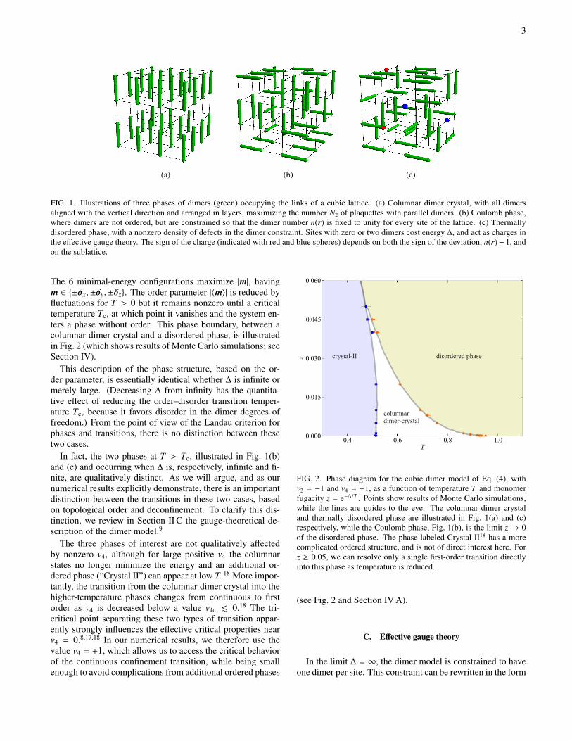
FIG. 1. Illustrations of three phases of dimers (green) occupying the links of a cubic lattice. (a) Columnar dimer crystal, with all dimers

aligned with the vertical direction and arranged in layers, maximizing the number N2 of plaquettes with parallel dimers. (b) Coulomb phase,

where dimers are not ordered, but are constrained so that the dimer number n(r) is fixed to unity for every site of the lattice. (c) Thermally

disordered phase, with a nonzero density of defects in the dimer constraint. Sites with zero or two dimers cost energy ∆, and act as charges in

the effective gauge theory. The sign of the charge (indicated with red and blue spheres) depends on both the sign of the deviation, n(r)− 1, and

on the sublattice.

The 6 minimal-energy configurations maximize |m|, having

m ∈ {±δx,±δy,±δz}. The order parameter |〈m〉| is reduced by

fluctuations for T > 0 but it remains nonzero until a critical

temperature Tc, at which point it vanishes and the system en-

ters a phase without order. This phase boundary, between a

columnar dimer crystal and a disordered phase, is illustrated

in Fig. 2 (which shows results of Monte Carlo simulations; see

Section IV).

This description of the phase structure, based on the or-

der parameter, is essentially identical whether ∆ is infinite or

merely large. (Decreasing ∆ from infinity has the quantita-

tive effect of reducing the order–disorder transition temper-

ature Tc, because it favors disorder in the dimer degrees of

freedom.) From the point of view of the Landau criterion for

phases and transitions, there is no distinction between these

two cases.

In fact, the two phases at T > Tc, illustrated in Fig. 1(b)

and (c) and occurring when ∆ is, respectively, infinite and fi-

nite, are qualitatively distinct. As we will argue, and as our

numerical results explicitly demonstrate, there is an important

distinction between the transitions in these two cases, based

on topological order and deconfinement. To clarify this dis-

tinction, we review in Section II C the gauge-theoretical de-

scription of the dimer model.9

The three phases of interest are not qualitatively affected

by nonzero v4, although for large positive v4 the columnar

states no longer minimize the energy and an additional or-

dered phase (“Crystal II”) can appear at low T .18 More impor-

tantly, the transition from the columnar dimer crystal into the

higher-temperature phases changes from continuous to first

order as v4 is decreased below a value v4c . 0.18 The tri-

critical point separating these two types of transition appar-

ently strongly influences the effective critical properties near

v4 = 0.8,17,18 In our numerical results, we therefore use the

value v4 = +1, which allows us to access the critical behavior

of the continuous confinement transition, while being small

enough to avoid complications from additional ordered phases

0.4 0.6 0.8 1.0T

0.000

0.015

0.030

0.045

0.060

z disordered phasecrystal-II

columnardimer-crystal

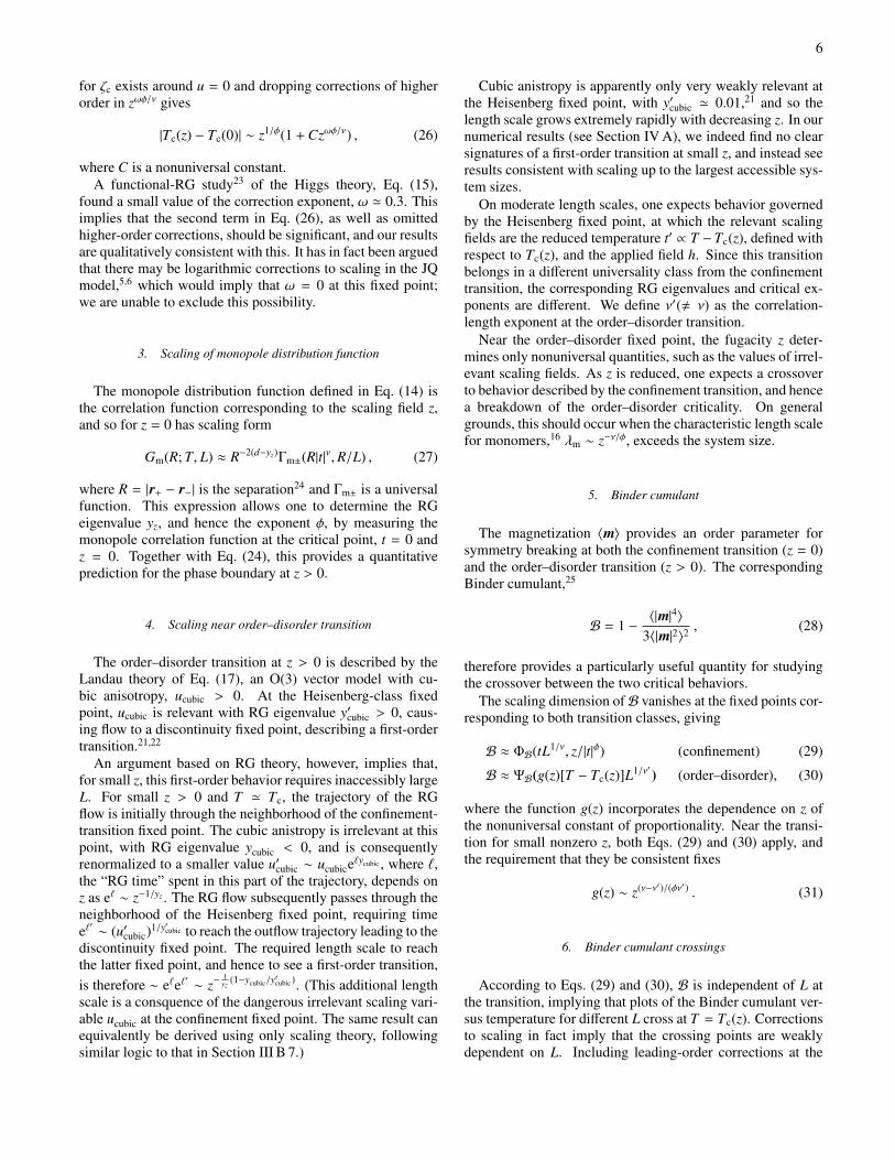
FIG. 2. Phase diagram for the cubic dimer model of Eq. (4), with

v2 = −1 and v4 = +1, as a function of temperature T and monomer

fugacity z = e−∆/T . Points show results of Monte Carlo simulations,

while the lines are guides to the eye. The columnar dimer crystal

and thermally disordered phase are illustrated in Fig. 1(a) and (c)

respectively, while the Coulomb phase, Fig. 1(b), is the limit z → 0

of the disordered phase. The phase labeled Crystal II18 has a more

complicated ordered structure, and is not of direct interest here. For

z ≥ 0.05, we can resolve only a single first-order transition directly

into this phase as temperature is reduced.

(see Fig. 2 and Section IV A).

C. Effective gauge theory

In the limit ∆ = ∞, the dimer model is constrained to have

one dimer per site. This constraint can be rewritten in the form

4

of a Gauss law by defining a “magnetic field”9,10

Bµ(r) = ηr

[

dµ(r) −1

z

]

, (7)

where z = 6 is the coordination number, and ηr = (−1)∑

µ rµ is

±1 on the two sublattices. The lattice divergence, defined by

divr B ≡∑

µ

[Bµ(r) − Bµ(r − δµ)] , (8)

obeys

divr B = ηr[n(r) − 1] , (9)

and so monomers act as charges (“magnetic monopoles”),

with sign depending on the sublattice.

In these terms, the partition function can be rewritten as

Z =∑

{Bµ(r)}

|divr B|≤1

e−Edimer/T∏

r

z(divr B)2

, (10)

where z = e−∆/T is the monomer fugacity. In particular, when

∆ = ∞, z = 0, and so

Z =∑

{Bµ(r)}

divr B=0

e−Edimer/T . (11)

The configurations to which the system is constrained at

z = 0, viz. those of close-packed, hard-core dimers, satisfy a

lattice Gauss law, divr B = 0. Such a constraint is preserved

by an appropriately chosen RG procedure, and is therefore ex-

pected to have important consequences for the long-distance

physics, qualitatively distinguishing the cases with z = 0 and

z > 0.

More explicitly, the result of such a procedure is to replace

Bµ(r) by a coarse-grained continuum vector field B(r) with a

corresponding constraint on its continuum divergence, ∇ ·B =

0. In the Coulomb phase at T > Tc, where B(r) continues

to fluctuate subject to this constraint, the effective continuum

action density is

Lgauge =1

2K|B|2 =

1

2K|∇ × A|2 , (12)

where B = ∇ × A. This is a (Gaussian) fixed point under

the RG, at which all other analytic terms are irrelevant, and at

which correlations are algebraic.9,10

While higher-order terms are irrelevant, and a mass term

for A is forbidden by gauge invariance, monomer fugacity is

a relevant perturbation at the Coulomb-phase fixed point. For

any nonzero z, the algebraic correlations are cut off at a length

scale ∝ z−1/d set by the monomer separation.

D. Confinement and deconfinement

The magnetization m is a local quantity that provides a con-

ventional order parameter for the low-temperature phase. At

z = 0, the phase transition can alternatively be characterized

through the concept of confinement.

Consider first the partition function of Eq. (11), but evalu-

ated in the presence of a set of charges at fixed positions,

Z[Qr] =∑

{Bµ(r)}

divr B=Qr

e−Edimer/T . (13)

The “monopole distribution function” Gm can then be defined,

in terms of a test pair of oppositely charged monomers at r±,

as

Gm(r+, r−) =Z[δr,r+ − δr,r− ]

Z. (14)

The function Gm can be considered as the correlation function

corresponding to the monomer fugacity.16 It is related to the

effective interaction, Um = −T ln Gm(r+, r−) induced between

the monomers as a result of the fluctuating dimers.

To understand the behavior of Gm, imagine starting in a

defect-free system and taking out a single dimer. This leaves

two vacant sites, which are on opposite sublattices and hence

carry opposite gauge charge. One can move each monomer by

rearranging the dimers; all local rearrangements preserve the

signs of the charges. In the ordered phase, attempting to sep-

arate the monomers in this way leaves behind a trail of distur-

bance, costing an energy (at least) proportional to its length, so

Um ∝ R = |r+ − r−|. In the Coulomb phase, there is no order

and so moving the monomers simply scrambles an already-

disordered background, leaving no such trail. The scrambling

induces only an entropic interaction; the monomers act like

point charges in the effective magnetic field, and Um obeys

the Coulomb law, Um ∝ R−1.

For z = 0, the large-separation limit of Gm is therefore qual-

itatively distinct in the phases on either side of Tc. In the or-

dered phase at T < Tc, the monomers are confined, costing an

unbounded energy to be separated to infinity, and so Gm → 0.

In the Coulomb phase at T > Tc, Um has a finite limit, and so

they are deconfined, with a nonzero limit for Gm.

This distinction applies only for z = 0; for nonzero

monomer fugacity, charges are screened in the limit of large

separation, and Um always approaches a finite constant for

large separation.

III. PHASE TRANSITIONS

A. Critical theories

We are interested in the phase transition from the dimer

crystal, with order parameter 〈m〉 , 0, into phases in which

the magnetization vanishes.

At z = 0, symmetry-breaking order appears simultane-

ously with the confinement of monomers, and both of these

effects must be incorporated in a critical theory. It has pre-

viously been argued12–14 that the transition is described by a

Higgs theory of a noncompact U(1) gauge field A and SU(2)-

5

symmetric matter fields ϕ. The action density is

Lcritical = Lgauge +Lmatter +Lmatter–gauge

Lmatter = s|ϕ|2 + u(|ϕ|2)2

Lmatter–gauge = |(∇ − iA)ϕ|2 ;

(15)

the pure-gauge part of the actionLgauge is as given in Eq. (12).

Note that the matter field ϕ is minimally coupled to A and so,

in the language where B = ∇ × A is the magnetic field, has

electric charge.19

The transition occurs when s is tuned through its critical

value sc. For s < sc, corresponding to the lower-temperature

phase, ϕ condenses and A acquires an effective mass term

by the Anderson–Higgs mechanism. This in turn eliminates

the algebraic correlations and confines the monomers (mag-

netic charges) through the Meissner effect. Symmetry ar-

guments show that the magnetization order parameter obeys

mµ ∼ ϕ†σµϕ, where σµ is a Pauli matrix, and so becomes

nonzero when ϕ condenses. The continuous SU(2) symmetry

of Lcritical is broken by an eighth-order (in ϕ) term,

Lcubic = −ucubic

∑

µ

m4µ , (16)

which is irrelevant at the critical point, but for s < sc selects

states where 〈m〉 is aligned with one of the 6 cubic directions

(ucubic > 0).

For z > 0, we instead expect the transition, between the

ordered dimer crystal and the thermally disordered phase, to

be described by a conventional Landau theory. The order pa-

rameter is the 3-component vector 〈m〉, which preferentially

aligns with one of the six cubic directions. The Landau action

is therefore given by

LLandau = |∇m|2 + sm|m|2+ um(|m|2)2

+Lcubic , (17)

where Lcubic is the cubic-anisotropy term given in Eq. (16),

again with ucubic > 0.20 This theory can be viewed as the re-

sult of adding a nonzero density of magnetic monopoles to

Eq. (15), suppressing the algebraic correlations of the gauge

field A and confining the matter field ϕ into the charge-neutral

bilinear m.

In this case, the anisotropy Lcubic is only quartic in the crit-

ical field m, and is known to be relevant. For ucubic = 0, the

transition would be continuous and in the Heisenberg univer-

sality class, but ucubic > 0 is expected to drive it first order.21

(In fact, this transition appears to be at most very weakly first-

order; see Sections III B 4 and IV A.)

B. Scaling

The presence of the continuous confinement transition at

z = 0 and T = Tc(z = 0) implies that the behavior in its

neighborhood is governed by the properties of the correspond-

ing RG fixed point. This includes along the transition line at

T = Tc(z > 0), and in particular determines the shape of the

phase boundary as a function of z. In addition, the first-order

nature of the transition at z > 0 is apparently weak enough

that, as we argue in Section III B 4, scaling theory can be ap-

plied to this transition. These observations lead to a number

of quantitative predictions that we are able to test in our sim-

ulations.

1. Scaling near confinement transition

Previous work15,16 has shown that, in addition to the re-

duced temperature

t =T − Tc(0)

Tc(0), (18)

there is a relevant scaling field at the confinement-transition

fixed point given by the monomer fugacity z. The reduced

free-energy density f = −L−d lnZ therefore has a singular

part obeying22

fs(t, z, h, L) ≈ |t|2−αΦ±(z/|t|φ, L|t|ν, h/|t|2−α−β) , (19)

where Φ± is a universal function, with the subscript ± indi-

cating dependence on the sign of t. For completeness an ap-

plied field h coupling to the magnetization has been included;

unless stated otherwise we set h = 0 in the following. The

exponents α, β, ν, and φ are related to the RG eigenvalues yt,

yz, and yh by

α = 2 −d

yt

(20)

β =d − yh

yt

(21)

ν =1

yt

(22)

φ =yz

yt

. (23)

2. Phase boundary

The phase boundary at T = Tc(z) is a nonanalyticity of

the free energy (for L = ∞), and hence of Φ− [since Tc(z) <

Tc(0)]. According to Eq. (19), this boundary has the form

|Tc(z) − Tc(0)| ∼ z1/φ . (24)

While this result is asymptotically exact, there are sub-

stantial corrections for nonzero z that must be incorporated

for a correct interpretation of the numerical data. The most

important comes from the leading irrelevant scaling variable

at the fixed point, which we denote u, with RG eigenvalue

yu = −ω < 0. Incorporating the unknown, nonuniversal con-

stant u into Eq. (19), while setting L = ∞ for simplicity, we

can write

fs(t, z) ≈ |t|2−αΦ±(z/|t|φ, uzωφ/ν) . (25)

The value ζc of ζ = z/|t|φ at which Φ− has a nonanalyticity is

now dependent on uzωφ/ν. Assuming that a Taylor expansion

6

for ζc exists around u = 0 and dropping corrections of higher

order in zωφ/ν gives

|Tc(z) − Tc(0)| ∼ z1/φ(1 +Czωφ/ν) , (26)

where C is a nonuniversal constant.

A functional-RG study23 of the Higgs theory, Eq. (15),

found a small value of the correction exponent, ω ≃ 0.3. This

implies that the second term in Eq. (26), as well as omitted

higher-order corrections, should be significant, and our results

are qualitatively consistent with this. It has in fact been argued

that there may be logarithmic corrections to scaling in the JQ

model,5,6 which would imply that ω = 0 at this fixed point;

we are unable to exclude this possibility.

3. Scaling of monopole distribution function

The monopole distribution function defined in Eq. (14) is

the correlation function corresponding to the scaling field z,

and so for z = 0 has scaling form

Gm(R; T, L) ≈ R−2(d−yz)Γm±(R|t|ν,R/L) , (27)

where R = |r+ − r−| is the separation24 and Γm± is a universal

function. This expression allows one to determine the RG

eigenvalue yz, and hence the exponent φ, by measuring the

monopole correlation function at the critical point, t = 0 and

z = 0. Together with Eq. (24), this provides a quantitative

prediction for the phase boundary at z > 0.

4. Scaling near order–disorder transition

The order–disorder transition at z > 0 is described by the

Landau theory of Eq. (17), an O(3) vector model with cu-

bic anisotropy, ucubic > 0. At the Heisenberg-class fixed

point, ucubic is relevant with RG eigenvalue y′cubic > 0, caus-

ing flow to a discontinuity fixed point, describing a first-order

transition.21,22

An argument based on RG theory, however, implies that,

for small z, this first-order behavior requires inaccessibly large

L. For small z > 0 and T ≃ Tc, the trajectory of the RG

flow is initially through the neighborhood of the confinement-

transition fixed point. The cubic anistropy is irrelevant at this

point, with RG eigenvalue ycubic < 0, and is consequently

renormalized to a smaller value u′cubic ∼ ucubiceℓycubic , where ℓ,

the “RG time” spent in this part of the trajectory, depends on

z as eℓ ∼ z−1/yz . The RG flow subsequently passes through the

neighborhood of the Heisenberg fixed point, requiring time

eℓ′

∼ (u′cubic)1/y′cubic to reach the outflow trajectory leading to the

discontinuity fixed point. The required length scale to reach

the latter fixed point, and hence to see a first-order transition,

is therefore ∼ eℓeℓ′

∼ z− 1

yz(1−ycubic/y

′cubic)

. (This additional length

scale is a consquence of the dangerous irrelevant scaling vari-

able ucubic at the confinement fixed point. The same result can

equivalently be derived using only scaling theory, following

similar logic to that in Section III B 7.)

Cubic anistropy is apparently only very weakly relevant at

the Heisenberg fixed point, with y′cubic ≃ 0.01,21 and so the

length scale grows extremely rapidly with decreasing z. In our

numerical results (see Section IV A), we indeed find no clear

signatures of a first-order transition at small z, and instead see

results consistent with scaling up to the largest accessible sys-

tem sizes.

On moderate length scales, one expects behavior governed

by the Heisenberg fixed point, at which the relevant scaling

fields are the reduced temperature t′ ∝ T −Tc(z), defined with

respect to Tc(z), and the applied field h. Since this transition

belongs in a different universality class from the confinement

transition, the corresponding RG eigenvalues and critical ex-

ponents are different. We define ν′(, ν) as the correlation-

length exponent at the order–disorder transition.

Near the order–disorder fixed point, the fugacity z deter-

mines only nonuniversal quantities, such as the values of irrel-

evant scaling fields. As z is reduced, one expects a crossover

to behavior described by the confinement transition, and hence

a breakdown of the order–disorder criticality. On general

grounds, this should occur when the characteristic length scale

for monomers,16 λm ∼ z−ν/φ, exceeds the system size.

5. Binder cumulant

The magnetization 〈m〉 provides an order parameter for

symmetry breaking at both the confinement transition (z = 0)

and the order–disorder transition (z > 0). The corresponding

Binder cumulant,25

B = 1 −〈|m|4〉

3〈|m|2〉2, (28)

therefore provides a particularly useful quantity for studying

the crossover between the two critical behaviors.

The scaling dimension ofB vanishes at the fixed points cor-

responding to both transition classes, giving

B ≈ ΦB(tL1/ν, z/|t|φ) (confinement) (29)

B ≈ ΨB(g(z)[T − Tc(z)]L1/ν′ ) (order–disorder), (30)

where the function g(z) incorporates the dependence on z of

the nonuniversal constant of proportionality. Near the transi-

tion for small nonzero z, both Eqs. (29) and (30) apply, and

the requirement that they be consistent fixes

g(z) ∼ z(ν−ν′)/(φν′) . (31)

6. Binder cumulant crossings

According to Eqs. (29) and (30), B is independent of L at

the transition, implying that plots of the Binder cumulant ver-

sus temperature for different L cross at T = Tc(z). Corrections

to scaling in fact imply that the crossing points are weakly

dependent on L. Including leading-order corrections at the

7

order–disorder transition replaces Eq. (30) by

B ≈ ΨB(g(z)[T − Tc(z)]L1/ν′ )

+ L−ω′

u(z)ΨB(g(z)[T − Tc(z)]L1/ν′ ) , (32)

where ΨB is an unknown function, −ω′ is the RG eigenvalue

of the leading irrelevant scaling operator, and u(z) expresses

the dependence of its coefficient on z. Again requiring consis-

tency with Eq. (29), we find

u(z) ∼ z−ω′ν/φ . (33)

At this order, the Binder cumulants at L = L1 and L2 have a

crossing at T = T×(L1, L2) given by25,26

T×(L1, L2) − Tc(z) ∼u(z)

g(z)

L−ω′

2− L−ω

′

1

L1/ν′

1− L

1/ν′

2

. (34)

In applying this result to numerical data, it is convenient to fix

the ratio ρ = L2/L1; incorporating the z dependence of g(z)

and u(z) then gives

T×(L, ρL) − Tc(z) ∼ z−(1+ω′ν−ν/ν′)/φL−ω′−1/ν′ . (35)

For the confinement transition, one similarly finds

T×(L, ρL) − Tc(0) ∼ L−ω−1/ν (z = 0) . (36)

7. Slope of Binder cumulant at crossing

The derivative of the Binder cumulant, taken with respect

to T and evaluated at T = Tc(z), can be used to determine the

correlation-length exponents ν and ν′. At z = 0, one finds the

scaling result

∂B

∂T

∣

∣

∣

∣

∣

T=Tc(0)

∼ L1/ν . (37)

Similarly, for z > 0, the slope is

∂B

∂T

∣

∣

∣

∣

∣

T=Tc(z)

≈g(z)

Tc(0)

[

Ψ′B(0)L1/ν′

+ u(z)Ψ′B(0)L1/ν′−ω′]

, (38)

where the correction term from Eq. (32) has been included. In

both cases, the slope is proportional to L1/ν(′) in the limit of

large L.

The corrections in Eq. (38) have magnitude proportional to

u(z) and therefore become more significant for smaller z. In

agreement with the general considerations of Section III B 4,

breakdown of order–disorder scaling occurs for system size L

below λm ∼ z−ν/φ, when the “correction” becomes larger than

the zeroth-order term.

8. Flux stiffness

An additional quantity of interest at the confinement transi-

tion is the flux stiffness,8,27

K−1=

1

3L2

∑

r⊥,µ

〈[φµ(r⊥)]2〉 , (39)

where

φµ(r⊥) =∑

rrµ=r⊥

Bµ(r) (40)

is the net “magnetic flux” through a closed surface, spanning

the periodic boundaries, normal to δµ. The flux stiffness K−1

vanishes in the thermodynamic limit for z = 0 and T < Tc,

while it approaches a constant in the Coulomb phase.

At the confinement phase transition, the quantity LK−1 has

zero scaling dimension,8 and hence shows a similar crossing

point to the Binder cumulant and a scaling form

LK−1(t, z, L) ≈ ΦK(tL1/ν, z/|t|φ) . (41)

The scaling dimension of the flux stiffness is not similarly

fixed at the order–disorder transition and so, in contrast to the

case of the Binder cumulant, the crossing points of LK−1 do

not converge for z > 0.

IV. NUMERICAL RESULTS

We have studied the dimer model defined in Section II A

using a Monte Carlo method based on the directed loop

algorithm28 but adapted to allow for violations of the dimer

constraint. An update within the set of constrained dimer con-

figurations can be performed by shifting dimers along a closed

loop. To change the number of monomers, one shifts dimers

along an open path, creating or annihilating monomers at each

end. (This corresponds to adding a string of magnetic flux

with a monopole at each end.) Details of the algorithm are

given in the Appendix.

Simulations were performed on lattices with periodic

boundary conditions and L3 sites, with system sizes up to

L = 144.

A. Phase structure

The phase structure of the model at z = 0 has

previously been studied extensively using Monte Carlo

simulations.8,11,13,14,17,18 For v4 = 0, one finds only the

Coulomb phase and the columnar dimer crystal, while for

v4 > 0 an additional crystalline phase, denoted Crystal II,

occurs at low T .18 We are mainly interested in the phase

boundary between the Coulomb and columnar phases, which

is shifted by nonzero v4 but qualitatively unaffected.

The phase structure at nonzero z and v4 = +1 is shown in

Fig. 2. The transition temperature to the columnar dimer crys-

tal is reduced as z increases, while the transition into Crystal II

is largely unchanged. At larger z = zmax ≃ 0.5, the two phase

boundaries merge into a single first-order transition between

the disordered phase and Crystal II. This sets an upper limit of

zmax on the values of z at which the transition to the columnar

dimer crystal can be studied.

There is strong evidence that the transition at z = 0 is con-

tinuous for v4 > 0 but first order for v4 < v4c . 0.18 As

8

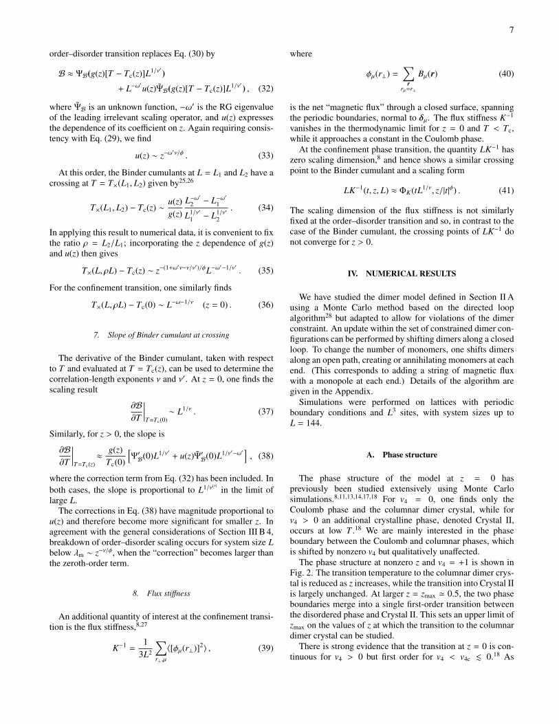
FIG. 3. Energy histograms from Monte Carlo simulations at z = 0

(left) and z = 10−2 (right). There is no indication of a double-peak

structure, which would indicate a first-order transition, within the

accuracy obtained in the simulations.

noted in Sections III A and III B 4, we expect that the transi-

tion at z > 0 is first order, but only very weakly so for small z.

Energy histograms close to the critical temperature, shown in

Fig. 3, exhibit no signs of the double-peak structure that would

indicate a first-order transition. The latent heat, if nonzero,

should grow with z, but only a single peak is resolvable (for

our largest available system sizes) up to the maximum acces-

sible z = zmax.

By contrast, for v4 = 0, a first-order transition is clearly

seen even for z ≃ 10−2. In this case, the effects of the tricritical

point at z = 0 and v4 = v4c are likely important18 and our

scaling conclusions are less reliable.

B. Confinement transition

We begin by reporting our results for the transition at z = 0

(and v4 = +1), which has previously been studied in Ref. 18.

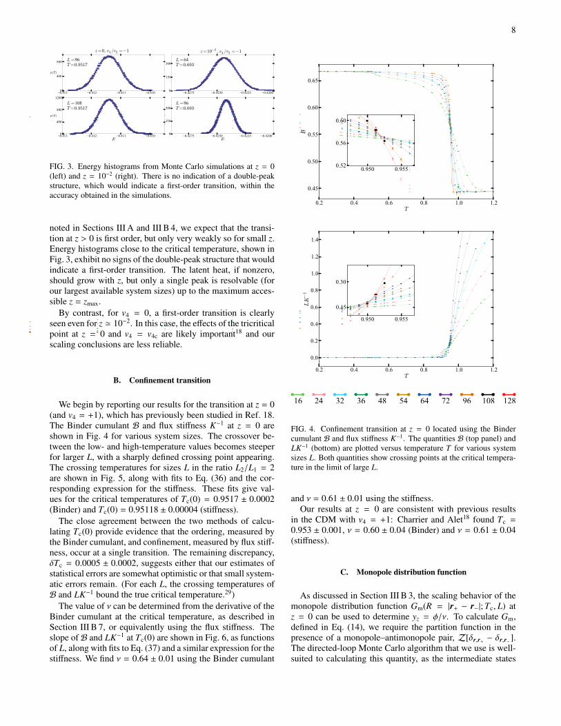
The Binder cumulant B and flux stiffness K−1 at z = 0 are

shown in Fig. 4 for various system sizes. The crossover be-

tween the low- and high-temperature values becomes steeper

for larger L, with a sharply defined crossing point appearing.

The crossing temperatures for sizes L in the ratio L2/L1 = 2

are shown in Fig. 5, along with fits to Eq. (36) and the cor-

responding expression for the stiffness. These fits give val-

ues for the critical temperatures of Tc(0) = 0.9517 ± 0.0002

(Binder) and Tc(0) = 0.95118 ± 0.00004 (stiffness).

The close agreement between the two methods of calcu-

lating Tc(0) provide evidence that the ordering, measured by

the Binder cumulant, and confinement, measured by flux stiff-

ness, occur at a single transition. The remaining discrepancy,

δTc = 0.0005 ± 0.0002, suggests either that our estimates of

statistical errors are somewhat optimistic or that small system-

atic errors remain. (For each L, the crossing temperatures of

B and LK−1 bound the true critical temperature.29)

The value of ν can be determined from the derivative of the

Binder cumulant at the critical temperature, as described in

Section III B 7, or equivalently using the flux stiffness. The

slope of B and LK−1 at Tc(0) are shown in Fig. 6, as functions

of L, along with fits to Eq. (37) and a similar expression for the

stiffness. We find ν = 0.64 ± 0.01 using the Binder cumulant

0.2 0.4 0.6 0.8 1.0 1.2T

0.45

0.50

0.55

0.60

0.65

B

0.950 0.9550.52

0.56

0.60

0.2 0.4 0.6 0.8 1.0 1.2T

0.0

0.2

0.4

0.6

0.8

1.0

1.2

1.4

LK−1

0.950 0.955

0.15

0.30

FIG. 4. Confinement transition at z = 0 located using the Binder

cumulant B and flux stiffness K−1. The quantities B (top panel) and

LK−1 (bottom) are plotted versus temperature T for various system

sizes L. Both quantities show crossing points at the critical tempera-

ture in the limit of large L.

and ν = 0.61 ± 0.01 using the stiffness.

Our results at z = 0 are consistent with previous results

in the CDM with v4 = +1: Charrier and Alet18 found Tc =

0.953 ± 0.001, ν = 0.60 ± 0.04 (Binder) and ν = 0.61 ± 0.04

(stiffness).

C. Monopole distribution function

As discussed in Section III B 3, the scaling behavior of the

monopole distribution function Gm(R = |r+ − r−|; Tc, L) at

z = 0 can be used to determine yz = φ/ν. To calculate Gm,

defined in Eq. (14), we require the partition function in the

presence of a monopole–antimonopole pair, Z[δr,r+ − δr,r− ].

The directed-loop Monte Carlo algorithm that we use is well-

suited to calculating this quantity, as the intermediate states

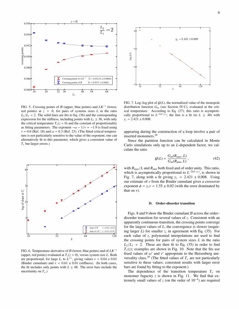
9

FIG. 5. Crossing points of B (upper, blue points) and LK−1 (lower,

red points) at z = 0, for pairs of systems sizes L in the ratio

L2/L1 = 2. The solid lines are fits to Eq. (36) and the corresponding

expression for the stiffness, including points with L1 ≥ 36, with only

the critical temperature Tc(z = 0) and the constant of proportionality

as fitting parameters. The exponent −ω − 1/ν = −1.9 is fixed using

ν = 0.6 (Ref. 18) and ω = 0.3 (Ref. 23). (The fitted critical tempera-

ture is not particularly sensitive to the value of the exponent; one can

alternatively fit to this parameter, which gives a consistent value of

Tc but larger errors.)

FIG. 6. Temperature-derivative ofB (lower, blue points) and of LK−1

(upper, red points) evaluated at Tc(z = 0), versus system size L. Both

are proportional, for large L, to L1/ν, giving values ν = 0.64 ± 0.01

(Binder cumulant) and ν = 0.61 ± 0.01 (stiffness). (In both cases,

the fit includes only points with L ≥ 48. The error bars include the

uncertainty on Tc.)

16 32 64 128L

7

6

5

4

log G( L

)

yz =2.421±0.008

FIG. 7. Log–log plot of G(L), the normalized value of the monopole

distribution function Gm (see Section IV C), evaluated at the crit-

ical temperature. According to Eq. (27), this ratio is asymptoti-

cally proportional to L−2(d−yz); the line is a fit (to L ≥ 48) with

yz = 2.421 ± 0.008.

appearing during the construction of a loop involve a pair of

inserted monomers.28

Since the partition function can be calculated in Monte

Carlo simulations only up to an L-dependent factor, we cal-

culate the ratio

G(L) =Gm(Rmax, L)

Gm(Rmin, L), (42)

with Rmax/L and Rmin both fixed and of order unity. This ratio,

which is asymptotically proportional to L−2(d−yz), is shown in

Fig. 7, along with a fit giving yz = 2.421 ± 0.008. Using

our estimate of ν from the Binder cumulant gives a crossover

exponent φ = yzν = 1.55 ± 0.02 (with the error dominated by

that on ν).

D. Order–disorder transition

Figs. 8 and 9 show the Binder cumulant B across the order–

disorder transition for several values of z. Consistent with an

apparently continuous transition, the crossing points converge

for the largest values of L; the convergence is slower (requir-

ing larger L) for smaller z, in agreement with Eq. (35). For

each value of z, polynomial interpolations are used to find

the crossing points for pairs of system sizes L in the ratio

L2/L1 = 2. These are then fit to Eq. (35) in order to find

Tc(z); examples are shown in Fig. 10. Note that the fits use

fixed values of ω′ and ν′ appropriate to the Heisenberg uni-

versality class.30 (The fitted values of Tc are not particularly

sensitive to these values; consistent results with larger error

bars are found by fitting to the exponent.)

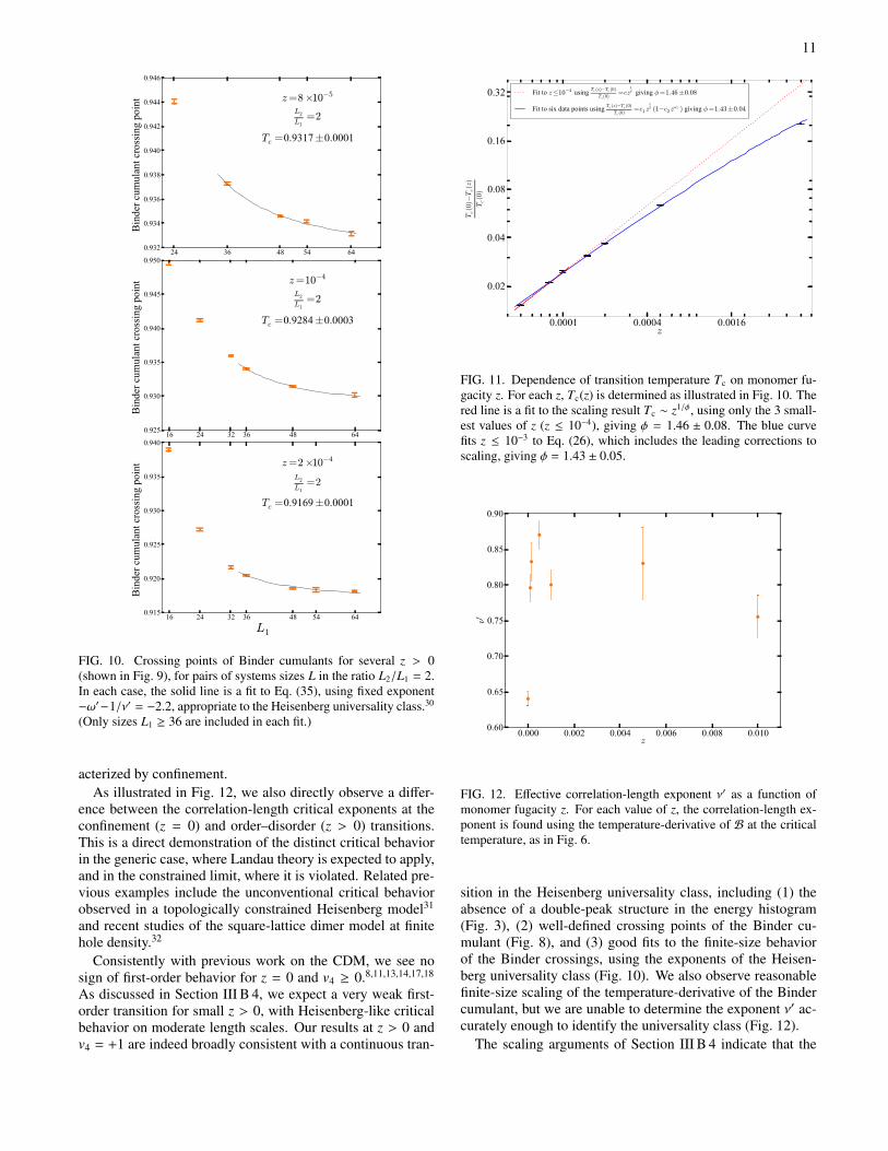
The dependence of the transition temperature Tc on

monomer fugacity z is shown in Fig. 11. We find that ex-

tremely small values of z (on the order of 10−4) are required

10

0.4 0.6 0.8 1.0T

0.48

0.54

0.60

0.66

B

z=10−3

0.86 0.88T

0.600

0.625

B

FIG. 8. Binder cumulant B as a function of T for z = 10−3. As for

z = 0 (Fig. 4), curves for different L cross at the critical temperature

(for L & 48), consistent with a continuous transition.

to give a power-law dependence of Tc(z), indicating that the

corrections to scaling are substantial. A power-law fit to the

smallest three z values, with z ≤ 10−4, gives φ = 1.46 ± 0.08,

which is in good agreement with the value φ = 1.55 ± 0.05

found using calculations at z = 0.

To incorporate leading-order corrections, we use Eq. (26),

with the value of the correction exponent ω = 0.3 found in a

functional-RG study23 of the critical action, Eq. (15). This in-

creases the range of z over which a reasonable fit is found;

we find a consistent value, φ = 1.43 ± 0.04, by including

z ≤ 10−3. (While the nominal error of the fit is reduced by

including data at larger z, the quoted value is not necessarily

reliable: The small magnitude of ω implies that significant

higher-order corrections should also be expected.)

E. Effective correlation-length exponent

The effective value of the correlation-length critical expo-

nent ν′, determined using the slope of B at Tc(z), is shown as

a function of z in Fig. 12. While a clear distinction is seen

between the exponents for z = 0 and z > 0, confirming the

different universality classes for these two cases, it is difficult

to draw further conclusions about the nature of the transition

at z > 0.

According to the scenario outlined in Sections III B 4 and

III B 7, one would expect ν′ to take the value30 νHeis. =

0.7112±0.0005 appropriate to the 3D Heisenberg universality

class, at least for intermediate values of z: For very small z,

the influence of the confinement fixed point gives corrections

(for even quite large L), described by Eq. (38); for larger z val-

ues the true first-order nature of the transition should become

apparent, causing complete breakdown of scaling. The large

FIG. 9. Binder cumulant B as a function of T for several z > 0. In

each case, a well-defined crossing point develops for large L, but the

convergence is slower for smaller z.

uncertainty in Tc(z), caused by slow convergence of the cross-

ings of the Binder cumulant, makes refinement of ν′ difficult.

V. CONCLUSIONS

Our central result, illustrated in Fig. 11, is the quantitative

relationship, derived using the scaling theory and confirmed in

large-scale Monte Carlo simulations, between the monopole

distribution function at z = 0 and the phase boundary at z > 0.

The connection between the two follows from their common

dependence on the RG eigenvalue yz of the monomer fugacity

at the fixed point describing the confinement transition. There

is no reason to expect such a relationship for a conventional

order–disorder transition, and so this result provides clear and

direct evidence for the claim of a non-Landau transition char-

11

FIG. 10. Crossing points of Binder cumulants for several z > 0

(shown in Fig. 9), for pairs of systems sizes L in the ratio L2/L1 = 2.

In each case, the solid line is a fit to Eq. (35), using fixed exponent

−ω′−1/ν′ = −2.2, appropriate to the Heisenberg universality class.30

(Only sizes L1 ≥ 36 are included in each fit.)

acterized by confinement.

As illustrated in Fig. 12, we also directly observe a differ-

ence between the correlation-length critical exponents at the

confinement (z = 0) and order–disorder (z > 0) transitions.

This is a direct demonstration of the distinct critical behavior

in the generic case, where Landau theory is expected to apply,

and in the constrained limit, where it is violated. Related pre-

vious examples include the unconventional critical behavior

observed in a topologically constrained Heisenberg model31

and recent studies of the square-lattice dimer model at finite

hole density.32

Consistently with previous work on the CDM, we see no

sign of first-order behavior for z = 0 and v4 ≥ 0.8,11,13,14,17,18

As discussed in Section III B 4, we expect a very weak first-

order transition for small z > 0, with Heisenberg-like critical

behavior on moderate length scales. Our results at z > 0 and

v4 = +1 are indeed broadly consistent with a continuous tran-

0.0001 0.0004 0.0016z

0.02

0.04

0.08

0.16

0.32

Tc(0)−

Tc(z)

Tc(0)

Fit to z≤10−4 using Tc (z)−Tc (0)

Tc (0)=cz

1φ giving φ=1.46±0.08

Fit to six data points using Tc (z)−Tc (0)

Tc (0)=c1 z

1φ (1−c2 zωz ) giving φ=1.43±0.04

FIG. 11. Dependence of transition temperature Tc on monomer fu-

gacity z. For each z, Tc(z) is determined as illustrated in Fig. 10. The

red line is a fit to the scaling result Tc ∼ z1/φ, using only the 3 small-

est values of z (z ≤ 10−4), giving φ = 1.46 ± 0.08. The blue curve

fits z ≤ 10−3 to Eq. (26), which includes the leading corrections to

scaling, giving φ = 1.43 ± 0.05.

0.000 0.002 0.004 0.006 0.008 0.010z

0.60

0.65

0.70

0.75

0.80

0.85

0.90

ν′

FIG. 12. Effective correlation-length exponent ν′ as a function of

monomer fugacity z. For each value of z, the correlation-length ex-

ponent is found using the temperature-derivative of B at the critical

temperature, as in Fig. 6.

sition in the Heisenberg universality class, including (1) the

absence of a double-peak structure in the energy histogram

(Fig. 3), (2) well-defined crossing points of the Binder cu-

mulant (Fig. 8), and (3) good fits to the finite-size behavior

of the Binder crossings, using the exponents of the Heisen-

berg universality class (Fig. 10). We also observe reasonable

finite-size scaling of the temperature-derivative of the Binder

cumulant, but we are unable to determine the exponent ν′ ac-

curately enough to identify the universality class (Fig. 12).

The scaling arguments of Section III B 4 indicate that the

12

TABLE I. Comparison of critical exponents for the cubic dimer

model and the JQ model3 with SU(2) symmetry, on square and hon-

eycomb lattices. For the CDM, two values of ν are reported in each

case, calculated using the Binder cumulant B and the stiffness K. In

this work, two values of yz are found, using the test-monopole dis-

tribution Gm at z = 0 and the phase boundary Tc(z > 0). For the JQ

model, the monopole scaling dimension yz is found using the anoma-

lous dimension of the VBS operator2 ηVBS = d + 2 − 2yz (denoted ηd

in Ref. 4 and ηΨ in Ref. 7). The two sets of values for the JQ model

on the square lattice correspond to two choices for the Q term.4 In

Ref. 7 good finite-size scaling is observed for both square and hon-

eycomb lattices (for system sizes L ≤ 96), but no uncertainties are

quoted.

Model ν ηVBS yz

this work CDM (v4 = +1)0.64(1) (B) 2.421(8) (Gm)

0.61(1) (K) 2.28(13) (Tc)

Ref. 18 CDM (v4 = +1)0.60(4) (B)

0.61(4) (K)

Ref. 4 JQ (square)0.67(1) 0.20(2) 2.40(1)

0.69(2) 0.20(2) 2.40(1)

Ref. 6 JQ (honeycomb) 0.54(5) 0.28(8) 2.36(4)

Ref. 7 JQ 0.59 0.35 2.33

putative first-order transition at z > 0 may never be visible

with realistic system sizes. Given the substantial corrections

to scaling exhibited by this transition, however, such argu-

ments should not be considered definitive. Indeed, at v4 = 0,

where corrections due to the tricritical point at v4 = v4c are sig-

nificant, clear first-order behavior is seen at z = 10−2. More

work, including studies at intermediate v4, are needed to clar-

ify this picture.

Universality and deconfined criticality

The zero-temperature ordering transition in certain 2D

quantum antiferromagnets, such as the [SU(2)] JQ model,3 is

claimed2 to be described by the same critical theory as given

in Eq. (15), and should therefore belong in the same universal-

ity class. Universality is one of the most remarkable features

of critical behavior, and a clear demonstration in the context

of non-Landau criticality would be a striking result. Since the

confinement transition in the dimer model necessarily occurs

at zero monomer density, it would also provide direct evidence

for deconfinement at the quantum critical point.

In the JQ model, the formation of a valence-bond solid

(VBS) is a consequence of the condensation of monopoles.2

The exponent ηVBS describing the appearance of VBS order

is therefore related to the monopole scaling dimension yz by

ηVBS = d+2−2yz. Values for yz and for the critical exponent ν,

displayed in Table I, show reasonable agreement, albeit with

large error bars.

While quantitative comparison of exponents is always chal-

lenging, it is made even more so in this case by the presence

of large corrections to scaling. Significant corrections are ob-

served in all cases,5 providing a further, qualitative indication

of universality. This indicates the presence of a weakly irrele-

vant scaling variable at the fixed point, an observation consis-

tent with a recent functional-RG study23 of the critical action

Eq. (15), which found a small correction-to-scaling exponent,

ω ≃ 0.3.

Although scaling behavior is visible over a range of length

scales,33 the possibility remains that the transition in the JQ

model is first order.34 (This should not be confused with the

weak first-order transition expected in the CDM at z > 0.

Berry phases suppress singly-charged monopoles in the JQ

model,2 so the transition is effectively at zero fugacity, z = 0.)

Indeed, a drift in the effective exponent values with increasing

system sizes was observed by Harada et al.,7 consistent with

a weak first-order transition. Universality between different

models and different lattices, as suggested by Table I, would

nonetheless imply that the RG flow is through the neighbor-

hood of a critical fixed point. In this case, one might expect

that, as in the CDM,17,18 additional perturbations could drive

the JQ transition truly continuous, or at least extend the length

scale over which scaling can be observed.

ACKNOWLEDGMENTS

The simulations were performed on resources provided by

the Swedish National Infrastructure for Computing (SNIC) at

the National Supercomputing Centre (NSC) and High Perfor-

mance Computing Center North (HPC2N).

Appendix: Monte Carlo algorithm

In this Appendix, we give a brief description of the numer-

ical methods used for the calculation.

The Monte Carlo routine is based on the directed loop

algorithm,28 adapted to allow for violations of dimer con-

straints. The system consists of a three dimensional cubic

lattice with L sites, or nodes, in each direction and periodic

boundary conditions. The dimers can occupy the links of

the lattice subject to the dimer constraints described in Sec-

tion II A. The Monte Carlo algorithm samples the equilibrium

thermodynamic distribution of dimer configurations ∝ exp− ET

where the energy E of a configuration is given by Eq. (4).

Two kinds of updates are used for sampling the configura-

tions; the first has a high acceptance rate but does not alter

the number of monomers, while the second can generate and

annihilate monomers.

The first kind of update begins by randomly picking a

monomer-free node P. The node is accepted with a proba-

bility (specified below) that depends only on the local config-

uration around P. If accepted, the system transitions into a

configuration in which there are two monomers—one on the

node P and one on a link connected to P. This is accompanied

by addition or removal of half a dimer as shown in the exam-

ple in Fig. 13. The link monomer has a “direction” attribute,

which serves to identify one of the two nodes connected to the

link as the node “ahead”, and which initially points away from

P.

13

b b b

b b b

b b b

b b b

b ⊗ b

b b b

b b b

b bc b

b b b

⊗bc

b b b

b bc b

b b b

⊗

, , etcP P P P

FIG. 13. First stage of a Monte Carlo update. After a node P is

selected, a sequence of dimer rearrangements is performed, starting

with creation of a pair of monomers of opposite charges—one on P

and one on a link connected to P. Half a dimer is added or removed

depending on the occupancy of the link.

b b b

b b b

b b b

⊗

bb

b

bb

b

bb

b⊗

bb

b

bb

b

bb

b⊗

b b b

b b b

b b b⊗, , etc

b b b

b b b

b b b

⊗

b b b

b b b

b b b⊗,

b b b

b b b

b b b

⊗

b b b

b bc b

b b b

bb

b

bb

bb

b⊗

b b b

b bc b

b b b

⊗

, , ...

⊗

bc

b b b

b b b

b b b

bb

b

b⊗

b

bb

b

bc, etc

FIG. 14. Examples of propagation of link monomer. Monomer prop-

agation in the first kind of update proceeds without changing the

monomer count on the nodes. If the node ahead has a monomer on it

(bottom), the update sequence can terminate with the link-monomer

annihilating the one on the node.

The link monomer can hop to one of the six links connected

to the node P1 ahead of it, erasing or creating dimers in the

process as shown in Fig. 14. Any such hopping that does not

result in a change in the number of monomers on P1 is al-

lowed. If the link monomer hops back to the same edge, the

direction of propagation is flipped. If P1 has a monomer, the

link monomer can annihilate with the one on the node, thereby

terminating the update process.

The probability of a transition from configuration k to q is

given by

p(k → q) =wq − δkq min(w)∑

w −min(w), (A.1)

where wi = exp(

−Ei

T

)

with Ei the energy of the configuration

without considering the two monomers created by the update

process. The energy of the half dimer is taken to be half that

of a full dimer at the same edge.

The second kind of update is similar to the first, but can

start on any node, including ones with monomers. Such an

update can terminate with the absorption of the link monomer

into a node, creating or annihilating a node monomer. The

propagation of the link monomer proceeds similarly to the

first update, with probability of transition from k to q of

p(k → q) =wq−δkq min(w)∑

w−min(w)where wi = exp

(

−Ei

T

)

. Since the

number of monomers can change after the update, the energy

E is calculated with the energy of every node monomer added

by the process.

The relative frequency of the two kinds of update was

chosen to minimize the convergence time but otherwise did

not affect the outcomes. Thermalization of the system from

a monomer-free, fully ordered configuration was achieved

by performing the updates until approximately 6000 × L3

forward-propagation steps of the link monomer had been

achieved. Configuration samples were subsequently taken

once every ∼ L3 forward propagation steps. Averages and er-

ror estimates of thermal expectation values and their combina-

tions (e.g., Binder cumulants) were obtained by the blocking

method.

The crossing point of Binder cumulants B(L1,T ) and

B(L2,T ) for systems of size L1 and L2 was obtained by

first finding an approximate crossing point T× from a piece-

wise linear interpolation of the data. A better estimate T×was obtained by fitting the data in the temperature interval

T× ± 0.00375 to quadratics,

B(L1,T ) = B0 + M1 (T − T×) + A1 (T − T×)2

B(L2,T ) = B0 + M2 (T − T×) + A2 (T − T×)2(A.2)

(with fit parameters B0, A1,2, M1,2, and T×).

The T -derivative of the binder cumulant was found using a

fluctuation–response relation,

(

∂B

∂T

)

z

= −1

3T 2

〈|m|4〉

〈|m|2〉2

[

〈(Edimer − 〈Edimer〉)|m|4〉

〈|m|4〉

− 2〈(Edimer − 〈Edimer〉)|m|

2〉

〈|m|2〉

]

, (A.3)

where Edimer is the energy excluding the contribution from

monomers.

The Monte Carlo algorithm and its implementation were

tested using comparisons with previously published results

and, for small system sizes, simple alternative methods. For

L = 2, results were compared with the exact averages obtained

from the enumeration of all possible microscopic states. For

system size L = 4 and parameters v4 = 0 and z = 0.05, the

energy and susceptibility were compared with an elementary

Metropolis algorithm. In addition, the self consistency of the

slope of the Binder cumulants estimated using Eq. (A.3) and

from curve fitting through Binder cumulants supports the va-

lidity of the sampling algorithm.

14

1 L. D. Landau and E. M. Lifshitz, Statistical Physics, Butterworth–

Heinemann, New York (1999).2 T. Senthil, A. Vishwanath, L. Balents, S. Sachdev, and M. P.

A. Fisher, Science 303, 1490 (2004); T. Senthil, L. Balents, S.

Sachdev, A. Vishwanath, and M. P. A. Fisher, Phys. Rev. B 70,

144407 (2004).3 A. W. Sandvik, Phys. Rev. Lett. 98, 227202 (2007).4 J. Lou, A. W. Sandvik, and N. Kawashima, Phys. Rev. B 80,

180414(R) (2009).5 A. W. Sandvik, Phys. Rev. Lett. 104, 177201 (2010).6 S. Pujari, K. Damle, and F. Alet, Phys. Rev. Lett. 111, 087203

(2013).7 K. Harada, T. Suzuki, T. Okubo, H. Matsuo, J. Lou, H. Watanabe,

S. Todo, and N. Kawashima, arXiv:1307.0501 (unpublished).8 F. Alet, G. Misguich, V. Pasquier, R. Moessner, and J. L. Jacobsen,

Phys. Rev. Lett. 97, 030403 (2006).9 D. A. Huse, W. Krauth, R. Moessner, and S. L. Sondhi, Phys. Rev.

Lett. 91, 167004 (2003).10 C. L. Henley, Ann. Rev. Cond. Matt. Phys. 1, 179 (2010).11 G. Misguich, V. Pasquier, F. Alet, Phys. Rev. B 78, 100402(R)

(2008).12 S. Powell and J. T. Chalker, Phys. Rev. Lett. 101, 155702 (2008);

Phys. Rev. B 80, 134413 (2009).13 D. Charrier, F. Alet, and P. Pujol, Phys. Rev. Lett. 101, 167205

(2008).14 G. Chen, J. Gukelberger, S. Trebst, F. Alet, and L. Balents, Phys.

Rev. B 80, 045112 (2009).15 S. Powell, Phys. Rev. Lett. 109, 065701 (2012).16 S. Powell, Phys. Rev. B 87, 064414 (2013).17 S. Papanikolaou and J. J. Betouras, Phys. Rev. Lett. 104, 045701

(2010).18 D. Charrier and F. Alet, Phys. Rev. B 82, 014429 (2010).19 The dual language is used in Ref. 14, so our electric charges are

there referred to as magnetic monopoles.20 A term (∇ · m)2 is also consistent with symmetry, but is irrelevant

at the Heisenberg fixed point.21

21 J. M. Carmona, A. Pelissetto, and E. Vicari, Phys. Rev. B 61,

15136 (2000).22 J. Cardy, Scaling and Renormalization in Statistical Physics

(Cambridge University Press, Cambridge, UK, 1996).23 L. Bartosch, arXiv:1307.3276 (unpublished).24 This result is asymptotically correct for R large compared to the

lattice scale. The form of Eq. (15) implies that Gm is then isotropic

and sublattice independent.25 K. Binder, Z. Phys. B 43, 119 (1981).26 A. M. Ferrenberg and D. P. Landau, Phys. Rev. B 44, 5081 (1991).27 For z = 0, the lattice Gauss law implies that φµ(R) is independent

of R and so the sum over R is redundant.8

28 A. W. Sandvik and R. Moessner, Phys. Rev. B 73, 144504 (2006).29 Reduced size (with periodic boundaries) tends to increase the or-

dering temperature, and hence the Binder crossing point, because

it restricts fluctuations to those commensurate with the system

period.22 The stiffness is sensitive to only those fluctuations that

change the total magnetic flux through the system. Threading a

unit of flux is easier for a smaller system, and so one needs lower

temperature to suppress such fluctuations for smaller L.30 M. Campostrini, M. Hasenbusch, A. Pelissetto, P. Rossi, and E.

Vicari, Phys. Rev. B 65, 144520 (2002).31 O. I. Motrunich and A. Vishwanath, Phys. Rev. B 70, 075104

(2004).32 S. Papanikolaou, D. Charrier, and E. Fradkin, arXiv:1310.4173

(unpublished).33 K. Chen, Y. Huang, Y. Deng, A.B. Kuklov, N.V. Prokof’ev, and

B.V. Svistunov, Phys. Rev. Lett. 110, 185701 (2013).34 A.B. Kuklov, M. Matsumoto, N.V. Prokof’ev, B.V. Svistunov, and

M. Troyer, Phys. Rev. Lett. 101, 050405 (2008).