springerseriesin cm
TRANSCRIPT


Springer Series in 37ComputationalMathematics
Editorial BoardR. BankR.L. GrahamJ. StoerR. VargaH. Yserentant

Sergej RjasanowWolfgang Wagner
Stochastic Numericsfor theBoltzmann Equation
With 98 Figures
123
Sergej Rjasanow
Fachrichtung 6.1 – MathematikUniversität des SaarlandesPostfach 15115066041 SaarbrückenGermanyemail: [email protected]
Wolfgang Wagner
Weierstrass Institutefor Applied Analysis and StochasticsMohrenstr. 3910117 BerlinGermanye-mail: [email protected]
Library of Congress Control Number: 2005922826
Mathematics Subject Classification (2000): 65C05, 65C20, 65C35, 60K35,82C22, 82C40, 82C80
ISSN 0179-3632ISBN-10 3-540-25268-1 Springer Berlin Heidelberg New YorkISBN-13 978-3-540-25268-9 Springer Berlin Heidelberg New York
This work is subject to copyright. All rights are reserved, whether the whole or part of thematerial is concerned, specifically the rights of translation, reprinting, reuse of illustrations,recitation, broadcasting, reproduction on microfilm or in any other way, and storage in databanks. Duplication of this publication or parts thereof is permitted only under the provisionsof the German Copyright Law of September 9, 1965, in its current version, and permission foruse must always be obtained from Springer. Violations are liable for prosecution under theGerman Copyright Law.
Springer is a part of Springer Science+Business Mediaspringeronline.com
© Springer-Verlag Berlin Heidelberg 2005Printed in Germany
The use of general descriptive names, registered names, trademarks, etc. in this publicationdoes not imply, even in the absence of a specific statement, that such names are exempt fromthe relevant protective laws and regulations and therefore free for general use.
Cover design: design&production, HeidelbergTypeset by the authors using a Springer LATEX macro packagePrinted on acid-free paper 46/3142sz-5 4 3 2 1 0
Preface
Stochastic numerical methods play an important role in large scale compu-tations in the applied sciences. Such algorithms are convenient, since inher-ent stochastic components of complex phenomena can easily be incorporated.However, even if the real phenomenon is described by a deterministic equa-tion, the high dimensionality often makes deterministic numerical methodsintractable.
A stochastic procedure, called direct simulation Monte Carlo (DSMC)method, has been developed in the physics and engineering community sincethe sixties. This method turned out to be a powerful tool for numerical studiesof complex rarefied gas flows. It was successfully applied to problems rang-ing from aerospace engineering to material processing and nanotechnology.In many situations, DSMC can be considered as a stochastic algorithm forsolving some macroscopic kinetic equation. An important example is the clas-sical Boltzmann equation, which describes the time evolution of large systemsof gas molecules in the rarefied regime, when the mean free path (distancebetween subsequent collisions of molecules) is not negligible compared to thecharacteristic length scale of the problem. This means that either the meanfree path is big (space-shuttle design, vacuum technology), or the character-istic length is small (micro-device engineering). As the dimensionality of thisnonlinear integro-differential equation is high (time, position, velocity), itsnumerical treatment is a typical application field of Monte Carlo algorithms.
Intensive mathematical research on stochastic algorithms for the Boltz-mann equation started in the eighties, when techniques for studying the con-vergence of interacting particle systems became available. Since that timemuch progress has been made in the justification and further development ofthese numerical methods.
The purpose of this book is twofold. The first goal is to give a mathe-matical description of various classical DSMC procedures, using the theoryof Markov processes (in particular, stochastic interacting particle systems) asa unifying framework. The second goal is a systematic treatment of an ex-tension of DSMC, called stochastic weighted particle method (SWPM). This

VI Preface
method has been developed by the authors during the last decade. SWPM in-cludes several new features, which are introduced for the purpose of variancereduction (rare event simulation). Rigorous results concerning the approxi-mation of solutions to the Boltzmann equation by particle systems are given,covering both DSMC and SWPM. Thorough numerical experiments are per-formed, illustrating the behavior of systematic and statistical error as well asthe performance of the methods.
We restricted our considerations to monoatomic gases. In this case theintroduction of weights is a completely artificial approach motivated by nu-merical purposes. This is the point we wanted to emphasize. In other situa-tions, like gas flows with several types of molecules of different concentrations,weighted particles occur in a natural way. SWPM contains more degrees offreedom than we have implemented and tested so far. Thus, there is somehope that there will be further applications. Both DSMC and SWPM can beapplied to more general kinetic equations. Interesting examples are relatedto rarefied granular gases (inelastic Boltzmann equation) and to ideal quan-tum gases (Uehling-Uhlenbeck-Boltzmann equation). In both cases there arenon-Maxwellian equilibrium distributions. Other types of molecules (internaldegrees of freedom, electrical charge) and many other interactions (chemicalreactions, coagulation, fragmentation) can be treated.
The structure of the book is reflected in the table of contents. Chapter 1recalls basic facts from kinetic theory, mainly about the Boltzmann equation.Chapter 2 is concerned with Markov processes related to Boltzmann typeequations. A relatively general class of piecewise-deterministic processes is de-scribed. The transition to the corresponding macroscopic equation is sketchedheuristically. Chapter 3 describes the stochastic algorithms related to theBoltzmann equation. This is the largest part of the book. All componentsof the procedures are discussed in detail and a rigorous convergence theo-rem is given. Chapter 4 contains results of numerical experiments. First, thespatially homogeneous Boltzmann equation is considered. Then, a spatiallyone-dimensional test problem is studied. Finally, results are obtained for aspecific spatially two-dimensional test configuration. Some auxiliary resultsare collected in two appendixes.
The chapters are relatively independent of each other. Necessary notationsand formulas are usually repeated at the beginning of a chapter, instead ofcross-referring to other chapters. A list of main notations is given at the endof this Preface. Symbols from that list will be used throughout the book. Wemostly avoided citing literature in the main text. Instead, each of the firstthree chapters is completed by a section including bibliographic remarks. Anextensive (but naturally not exhaustive) list of references is given at the endof the book.
The idea to write this book came up in 1999, when we had completedseveral papers related to DSMC and SWPM. Our naive hope was to finish itrather quickly. In May 2001 this Preface contained only one remark – “sevenmonths left to deadline”. On the one hand, the long delay of three years was

Preface VII
sometimes annoying, but, on the other hand, we mostly enjoyed the intensivework on a very interesting subject. We would like to thank our colleagues fromthe kinetics community for many useful discussions and suggestions. We aregrateful to our home institutions, the University of Saarland in Saarbruckenand the Weierstrass Institute for Applied Analysis and Stochastics in Berlin,for providing an encouraging scientific environment. Finally, we are glad toacknowledge support by the Mathematical Research Institute Oberwolfach(RiP program) during an early stage of the project, and a research grant fromthe German Research Foundation (DFG).
Saarbrucken and Berlin Sergej RjasanowDecember 2004 Wolfgang Wagner

List of notations
R3 Euclidean space
(., .) scalar product in R3
|.| norm in R3
S2 unit sphere in R3
D open subset of R3
∂D boundary of Dn(x) unit inward normal vector at x ∈ ∂Dσ(dx) uniform surface measure (area) on ∂Dδ(x) Dirac’s delta-functionI identity matrixtr C trace of a matrix CvvT matrix with elements vivj for v ∈ R
3
∇x gradient with respect to x ∈ R3
div b(x) divergence of a vector function b on R3
E ξ expectation of a random variable ξVar ξ variance of a random variable ξB(X) Borel sets of a metric space XM(X) finite Borel measures on X
MV,T (v) =1
(2π T )3/2exp(−|v − V |2
2T
)Maxwell distribution, with v, V ∈ R
3 and T > 0R
3in(x) =
{v ∈ R
3 : (v, n(x)) > 0}
velocities leading a particle from x ∈ ∂D inside D
R3out(x) =
{v ∈ R
3 : (v, n(x)) < 0}
velocities leading a particle from x ∈ ∂D outside D
δi,j ={
1 , if i = j0 , otherwise
Kronecker’s symbol

X List of notations
δx(A) ={
1 , if x ∈ A0 , otherwise
Dirac measure, with x ∈ X and A ∈ B(X)
χA(x) ={
1 , if x ∈ A0 , otherwise
indicator function of a set A , with x ∈ X and A ⊂ X
||ϕ||∞ = supx∈X
|ϕ(x)|
for any measurable function ϕ on X
〈ϕ, ν〉 =∫
X
ϕ(x) ν(dx)
for any ν ∈ M(X) and ϕ such that ||ϕ||∞ < ∞

Contents
1 Kinetic theory . . . . . . . . . . . . . . . . . . . . . . . . . . . . . . . . . . . . . . . . . . . . . 11.1 The Boltzmann equation . . . . . . . . . . . . . . . . . . . . . . . . . . . . . . . . . 11.2 Collision transformations . . . . . . . . . . . . . . . . . . . . . . . . . . . . . . . . . 21.3 Collision kernels . . . . . . . . . . . . . . . . . . . . . . . . . . . . . . . . . . . . . . . . . 81.4 Boundary conditions . . . . . . . . . . . . . . . . . . . . . . . . . . . . . . . . . . . . . 111.5 Physical properties of gas flows . . . . . . . . . . . . . . . . . . . . . . . . . . . . 12
1.5.1 Physical quantities and units . . . . . . . . . . . . . . . . . . . . . . . . 121.5.2 Macroscopic flow properties . . . . . . . . . . . . . . . . . . . . . . . . . 131.5.3 Molecular flow properties . . . . . . . . . . . . . . . . . . . . . . . . . . . 141.5.4 Measurements . . . . . . . . . . . . . . . . . . . . . . . . . . . . . . . . . . . . 151.5.5 Air at standard conditions . . . . . . . . . . . . . . . . . . . . . . . . . . 15
1.6 Properties of the collision integral . . . . . . . . . . . . . . . . . . . . . . . . . 161.7 Moment equations . . . . . . . . . . . . . . . . . . . . . . . . . . . . . . . . . . . . . . . 211.8 Criterion of local equilibrium . . . . . . . . . . . . . . . . . . . . . . . . . . . . . 241.9 Scaling transformations . . . . . . . . . . . . . . . . . . . . . . . . . . . . . . . . . . 281.10 Comments and bibliographic remarks . . . . . . . . . . . . . . . . . . . . . . 30
2 Related Markov processes . . . . . . . . . . . . . . . . . . . . . . . . . . . . . . . . . 332.1 Boltzmann type piecewise-deterministic Markov processes . . . . 33
2.1.1 Free flow and state space . . . . . . . . . . . . . . . . . . . . . . . . . . . 332.1.2 Construction of sample paths . . . . . . . . . . . . . . . . . . . . . . . 342.1.3 Jump behavior . . . . . . . . . . . . . . . . . . . . . . . . . . . . . . . . . . . . 352.1.4 Extended generator . . . . . . . . . . . . . . . . . . . . . . . . . . . . . . . . 39
2.2 Heuristic derivation of the limiting equation . . . . . . . . . . . . . . . . 412.2.1 Equation for measures . . . . . . . . . . . . . . . . . . . . . . . . . . . . . 412.2.2 Equation for densities . . . . . . . . . . . . . . . . . . . . . . . . . . . . . . 432.2.3 Boundary conditions . . . . . . . . . . . . . . . . . . . . . . . . . . . . . . . 46
2.3 Special cases and bibliographic remarks . . . . . . . . . . . . . . . . . . . . 472.3.1 Boltzmann equation and boundary conditions . . . . . . . . . 472.3.2 Boltzmann type processes . . . . . . . . . . . . . . . . . . . . . . . . . . 482.3.3 History . . . . . . . . . . . . . . . . . . . . . . . . . . . . . . . . . . . . . . . . . . 55

XII Contents
3 Stochastic weighted particle method . . . . . . . . . . . . . . . . . . . . . . . 653.1 The DSMC framework . . . . . . . . . . . . . . . . . . . . . . . . . . . . . . . . . . . 67
3.1.1 Generating the initial state . . . . . . . . . . . . . . . . . . . . . . . . . 673.1.2 Decoupling of free flow and collisions . . . . . . . . . . . . . . . . . 683.1.3 Limiting equations . . . . . . . . . . . . . . . . . . . . . . . . . . . . . . . . 693.1.4 Calculation of functionals . . . . . . . . . . . . . . . . . . . . . . . . . . 69
3.2 Free flow part . . . . . . . . . . . . . . . . . . . . . . . . . . . . . . . . . . . . . . . . . . . 713.2.1 Modeling of boundary conditions . . . . . . . . . . . . . . . . . . . . 713.2.2 Modeling of inflow . . . . . . . . . . . . . . . . . . . . . . . . . . . . . . . . . 74
3.3 Collision part . . . . . . . . . . . . . . . . . . . . . . . . . . . . . . . . . . . . . . . . . . . 783.3.1 Cell structure . . . . . . . . . . . . . . . . . . . . . . . . . . . . . . . . . . . . . 783.3.2 Fictitious collisions . . . . . . . . . . . . . . . . . . . . . . . . . . . . . . . . 803.3.3 Majorant condition . . . . . . . . . . . . . . . . . . . . . . . . . . . . . . . . 813.3.4 Global upper bound for the relative velocity norm . . . . . 833.3.5 Shells in the velocity space . . . . . . . . . . . . . . . . . . . . . . . . . 853.3.6 Temperature time counter . . . . . . . . . . . . . . . . . . . . . . . . . . 89
3.4 Controlling the number of particles . . . . . . . . . . . . . . . . . . . . . . . . 973.4.1 Collision processes with reduction . . . . . . . . . . . . . . . . . . . 973.4.2 Convergence theorem . . . . . . . . . . . . . . . . . . . . . . . . . . . . . . 993.4.3 Proof of the convergence theorem. . . . . . . . . . . . . . . . . . . . 1033.4.4 Construction of reduction measures . . . . . . . . . . . . . . . . . . 119
3.5 Comments and bibliographic remarks . . . . . . . . . . . . . . . . . . . . . . 1323.5.1 Some Monte Carlo history . . . . . . . . . . . . . . . . . . . . . . . . . . 1323.5.2 Time counting procedures . . . . . . . . . . . . . . . . . . . . . . . . . . 1323.5.3 Convergence and variance reduction . . . . . . . . . . . . . . . . . 1343.5.4 Nanbu’s method . . . . . . . . . . . . . . . . . . . . . . . . . . . . . . . . . . 1363.5.5 Approximation order . . . . . . . . . . . . . . . . . . . . . . . . . . . . . . 1403.5.6 Further references . . . . . . . . . . . . . . . . . . . . . . . . . . . . . . . . . 145
4 Numerical experiments . . . . . . . . . . . . . . . . . . . . . . . . . . . . . . . . . . . . 1474.1 Maxwellian initial state . . . . . . . . . . . . . . . . . . . . . . . . . . . . . . . . . . 149
4.1.1 Uniform approximation of the velocity space . . . . . . . . . . 1504.1.2 Stability of moments . . . . . . . . . . . . . . . . . . . . . . . . . . . . . . . 1504.1.3 Tail functionals . . . . . . . . . . . . . . . . . . . . . . . . . . . . . . . . . . . 1514.1.4 Hard sphere model . . . . . . . . . . . . . . . . . . . . . . . . . . . . . . . . 156
4.2 Relaxation of a mixture of two Maxwellians . . . . . . . . . . . . . . . . . 1574.2.1 Convergence of DSMC . . . . . . . . . . . . . . . . . . . . . . . . . . . . . 1594.2.2 Convergence of SWPM . . . . . . . . . . . . . . . . . . . . . . . . . . . . . 1614.2.3 Tail functionals . . . . . . . . . . . . . . . . . . . . . . . . . . . . . . . . . . . 1644.2.4 Hard sphere model . . . . . . . . . . . . . . . . . . . . . . . . . . . . . . . . 169
4.3 BKW solution of the Boltzmann equation . . . . . . . . . . . . . . . . . . 1714.3.1 Convergence of moments . . . . . . . . . . . . . . . . . . . . . . . . . . . 1724.3.2 Tail functionals . . . . . . . . . . . . . . . . . . . . . . . . . . . . . . . . . . . 175
4.4 Eternal solution of the Boltzmann equation . . . . . . . . . . . . . . . . . 1784.4.1 Power functionals . . . . . . . . . . . . . . . . . . . . . . . . . . . . . . . . . 180

Contents XIII
4.4.2 Tail functionals . . . . . . . . . . . . . . . . . . . . . . . . . . . . . . . . . . . 1814.5 A spatially one-dimensional example . . . . . . . . . . . . . . . . . . . . . . . 181
4.5.1 Properties of the shock wave problem . . . . . . . . . . . . . . . . 1824.5.2 Mott-Smith model . . . . . . . . . . . . . . . . . . . . . . . . . . . . . . . . . 1854.5.3 DSMC calculations . . . . . . . . . . . . . . . . . . . . . . . . . . . . . . . . 1894.5.4 Comparison with the Mott-Smith model . . . . . . . . . . . . . . 1914.5.5 Histograms . . . . . . . . . . . . . . . . . . . . . . . . . . . . . . . . . . . . . . . 1944.5.6 Bibliographic remarks . . . . . . . . . . . . . . . . . . . . . . . . . . . . . . 197
4.6 A spatially two-dimensional example . . . . . . . . . . . . . . . . . . . . . . . 1984.6.1 Explicit formulas in the collisionless case . . . . . . . . . . . . . 2004.6.2 Case with collisions . . . . . . . . . . . . . . . . . . . . . . . . . . . . . . . . 2064.6.3 Influence of a hot wall . . . . . . . . . . . . . . . . . . . . . . . . . . . . . 2074.6.4 Bibliographic remarks . . . . . . . . . . . . . . . . . . . . . . . . . . . . . . 210
A Auxiliary results . . . . . . . . . . . . . . . . . . . . . . . . . . . . . . . . . . . . . . . . . . . 211A.1 Properties of the Maxwell distribution . . . . . . . . . . . . . . . . . . . . . 211A.2 Exact relaxation of moments . . . . . . . . . . . . . . . . . . . . . . . . . . . . . . 213A.3 Properties of the BKW solution . . . . . . . . . . . . . . . . . . . . . . . . . . . 217A.4 Convergence of random measures . . . . . . . . . . . . . . . . . . . . . . . . . . 220A.5 Existence of solutions . . . . . . . . . . . . . . . . . . . . . . . . . . . . . . . . . . . . 223
B Modeling of distributions . . . . . . . . . . . . . . . . . . . . . . . . . . . . . . . . . . 229B.1 General techniques . . . . . . . . . . . . . . . . . . . . . . . . . . . . . . . . . . . . . . 229
B.1.1 Acceptance-rejection method. . . . . . . . . . . . . . . . . . . . . . . . 229B.1.2 Transformation method . . . . . . . . . . . . . . . . . . . . . . . . . . . . 230B.1.3 Composition method . . . . . . . . . . . . . . . . . . . . . . . . . . . . . . . 231
B.2 Uniform distribution on the unit sphere . . . . . . . . . . . . . . . . . . . . 231B.3 Directed distribution on the unit sphere . . . . . . . . . . . . . . . . . . . . 232B.4 Maxwell distribution . . . . . . . . . . . . . . . . . . . . . . . . . . . . . . . . . . . . . 234B.5 Directed half-space Maxwell distribution . . . . . . . . . . . . . . . . . . . 236B.6 Initial distribution of the BKW solution . . . . . . . . . . . . . . . . . . . . 239B.7 Initial distribution of the eternal solution . . . . . . . . . . . . . . . . . . . 241
References . . . . . . . . . . . . . . . . . . . . . . . . . . . . . . . . . . . . . . . . . . . . . . . . . . . . . 243
Index . . . . . . . . . . . . . . . . . . . . . . . . . . . . . . . . . . . . . . . . . . . . . . . . . . . . . . . . . . 255
1
Kinetic theory
1.1 The Boltzmann equation
Kinetic theory describes a gas as a system of many particles (molecules) mov-ing around according to the laws of classical mechanics. Particles interact,changing their velocities through binary collisions. The gas is assumed to besufficiently dilute so that interactions involving more than two particles canbe neglected. In the simplest case all particles are assumed to be identical andno effects of chemistry or electrical charge are considered.
Since the number of gas molecules is huge (1019 per cm3 at standardconditions), it would be impossible to study the individual behavior of eachof them. Instead a statistical description is used, i.e., some function
f(t, x, v) , t ≥ 0 , x ∈ R3 , v ∈ R
3 , (1.1)
is introduced that represents the average number of gas particles at time thaving a position close to x and a velocity close to v . The basis for this statis-tical theory was provided in the second half of the 19th century. James ClerkMaxwell (1831-1879) found the distribution function of the gas molecule ve-locities in thermal equilibrium. Ludwig Boltzmann (1844-1906) studied theproblem if a gas starting from any initial state reaches the Maxwell distri-bution
feq(v) = [ m
2π k T
] 32
exp(−m |v − V |2
2 k T
), v ∈ R
3 , (1.2)
where , V, T are the density (number of molecules per unit volume), thestream velocity and the absolute temperature of the gas, m is the mass of amolecule and k is Boltzmann’s constant. In 1872 he established the equation
∂
∂tf(t, x, v) + (v,∇x) f(t, x, v) = (1.3)∫R3
dw
∫ ∞
0
r dr
∫ 2π
0
dϕ |v − w|[f(t, x, v′) f(t, x, w′)−f(t, x, v) f(t, x, w)
]

2 1 Kinetic theory
describing the time evolution of the distribution function (1.1). The collisiontransformation
v, w, r, ϕ −→ v′, w′ (1.4)
is determined by the interaction potential governing collisions and by therelative position of the molecules. This position is uniformly spread over theplane perpendicular to v − w and expressed via polar coordinates. The left-hand side of equation (1.3) corresponds to the free streaming of the particles,while the right-hand side corresponds to the binary collisions that may eitherincrease (gain term) or decrease (loss term) the number of particles withgiven position and velocity. The (perhaps slightly confusing) fact that the gainterm contains the post-collision velocities instead of the pre-collision velocities(leading to v, w) is due to symmetry of the interaction law. The conservationproperties for momentum and energy
v′ + w′ = v + w , |v′|2 + |w′|2 = |v|2 + |w|2 (1.5)
imply that the function (1.2) satisfies equation (1.3).
1.2 Collision transformations
Even in the simple case of hard sphere interaction (particles collide like billiardballs) an explicit expression of the collision transformation (1.4) would berather complicated. Therefore other forms are commonly used.
Assuming a spherically symmetric interaction law and using the centeredvelocities
v = v − v + w
2=
v − w
2, w = w − v + w
2=
w − v
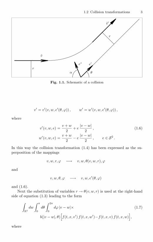
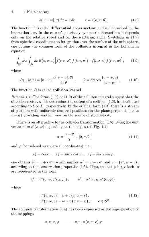
2a collision can be illustrated as shown in Fig. 1.1. The relative position ofthe colliding particles projected onto the plane perpendicular to their relativevelocity is parametrized in polar coordinates r, ϕ . The impact parameterr is the distance of closest approach of the two (point) particles had theycontinued their motion without interaction. Due to symmetry the angle ϕdoes not influence the collision transformation. The out-going velocities v′, w′
depend on the in-going velocities v, w and on the scattering angle θ ∈ [0, π] ,which is determined by the parameter r and the interaction law. The valuer = 0 corresponds to a central collision (scattering angle θ = π), while r → ∞corresponds to grazing collisions (scattering angle θ → 0). Using the unitvector e′ depending on θ and ϕ (considered as spherical coordinates), i.e.
e′1 = cos θ , e′2 = sin θ cos ϕ , e′3 = sin θ sin ϕ ,
one obtains v′ = c e′ , which implies w′ = −c e′ and c = |v′−w′|2 = |v−w|
2 ,according to the conservation properties (1.5). Thus, the out-going velocitiesare represented in the form
1.2 Collision transformations 3
Fig. 1.1. Schematic of a collision
r
r
θα
v
v′
e′e∗
v′ = v′(v, w, e′(θ, ϕ)) , w′ = w′(v, w, e′(θ, ϕ)) ,
where
v′(v, w, e) =v + w
2+ e
|v − w|2
, (1.6)
w′(v, w, e) =v + w
2− e
|v − w|2
, e ∈ S2 .
In this way the collision transformation (1.4) has been expressed as the su-perposition of the mappings
v, w, r, ϕ −→ v, w, θ(v, w, r), ϕ
and
v, w, θ, ϕ −→ v, w, e′(θ, ϕ)
and (1.6).Next the substitution of variables r → θ(v, w, r) is used at the right-hand
side of equation (1.3) leading to the form
∫R3
dw
∫ π
0
dθ
∫ 2π
0
dϕ |v − w|× (1.7)
b(|v − w|, θ)[f(t, x, v′) f(t, x, w′)−f(t, x, v) f(t, x, w)
],
where
4 1 Kinetic theory
b(|v − w|, θ) dθ = r dr , r = r(v, w, θ) . (1.8)
The function b is called differential cross section and is determined by theinteraction law. In the case of spherically symmetric interactions it dependsonly on the relative speed and on the scattering angle. Switching in (1.7)from spherical coordinates to integration over the surface of the unit sphere,one obtains the common form of the collision integral in the Boltzmannequation∫
R3dw
∫S2
deB(v, w, e)[f(t, x, v′) f(t, x, w′)−f(t, x, v) f(t, x, w)
], (1.9)
where
B(v, w, e) = |v − w| b(|v − w|, θ)sin θ
, θ = arccos(v − w, e)|v − w| . (1.10)
The function B is called collision kernel.
Remark 1.1. The forms (1.7) or (1.9) of the collision integral suggest that thedirection vector, which determines the output of a collision (1.6), is distributedaccording to b or B , respectively. In the original form (1.3) there is a streamof particles with uniformly smeared positions (in the plane perpendicular tov − w) providing another view on the source of stochasticity.
There is an alternative to the collision transformation (1.6). Using the unitvector e∗ = e∗(α,ϕ) depending on the angles (cf. Fig. 1.1)
α =π − θ
2∈ [0, π/2] (1.11)
and ϕ (considered as spherical coordinates), i.e.
e∗1 = cos α , e∗2 = sin α cos ϕ , e∗3 = sin α sin ϕ ,
one obtains v′ = v + c e∗ , which implies w′ = w − c e∗ and c = (e∗, w − v) ,according to the conservation properties (1.5). Thus, the out-going velocitiesare represented in the form
v′ = v∗(v, w, e∗(α,ϕ)) , w′ = w∗(v, w, e∗(α,ϕ)) ,
where
v∗(v, w, e) = v + e (e, w − v) , (1.12)w∗(v, w, e) = w + e (e, v − w) , e ∈ S2 .
The collision transformation (1.4) has been expressed as the superposition ofthe mappings
v, w, r, ϕ −→ v, w, α(v, w, r), ϕ

1.2 Collision transformations 5
and
v, w, α, ϕ −→ v, w, e∗(α,ϕ)
and (1.12).The substitution of variables r → α(v, w, r) at the right-hand side of equa-
tion (1.3) leads to the form∫R3
dw
∫ π2
0
dα
∫ 2π
0
dϕ |v − w|× (1.13)
b∗(|v − w|, α)[f(t, x, v∗) f(t, x, w∗)−f(t, x, v) f(t, x, w)
],
where
b∗(|v − w|, α) dα = r dr , r = r(v, w, α) . (1.14)
Switching in (1.13) from spherical coordinates to integration over the surfaceof the unit sphere, one obtains
(1.15)∫R3
dw
∫S2
+(w−v)
deB∗(v, w, e)[f(t, x, v∗) f(t, x, w∗)−f(t, x, v) f(t, x, w)
],
where
B∗(v, w, e) = |v − w| b∗(|v − w|, α)sin α
, α = arccos(w − v, e)|w − v| (1.16)
and (for u ∈ R3)
S2+(u) = {e ∈ S2 : (e, u) > 0} , S2
−(u) = {e ∈ S2 : (e, u) < 0} . (1.17)
Thus, there are two different forms (1.9) and (1.15) of the collision integral inthe Boltzmann equation, corresponding to the collision transformations (1.6)and (1.12).
Theorem 1.2. The collision kernels appearing in (1.9) and (1.15) are relatedto each other via
B∗(v, w, e) = 4 (e, u)B(v, w, 2 e (e, u) − u) (1.18)
and
B(v, w, e) =1
2√
2 (1 + (e, u))B∗(
v, w,e + u√
2 (1 + (e, u))
), (1.19)
where
u = u(v, w) =w − v
|w − v| , v = w .
6 1 Kinetic theory
Note that
|2 e (e, u) − u|2 = 1 and |e + u|2 = 2 (1 + (e, u)) = 2 (e + u, u) .
We prepare the proof by the following lemma.
Lemma 1.3. Let Φ be an appropriate test function and u ∈ S2 . Then (cf.(1.17))∫
S2Φ(e + u) de = 4
∫S2
+(u)
(e, u)Φ(2 e (e, u)) de (1.20)
= 4∫S2−(u)
|(e, u)|Φ(2 e (e, u)) de = 2∫S2
|(e, u)|Φ(2 e (e, u)) de .
Proof. Introducing spherical coordinates ϕ1 ∈ [0, π] , ϕ2 ∈ [0, 2π] suchthat
e1 = cos ϕ1 , e2 = sin ϕ1 cos ϕ2 , e3 = sin ϕ1 sin ϕ2
and u = (1, 0, 0) , one obtains∫S2
Φ(e + u) de = (1.21)∫ π
0
dϕ1
∫ 2π
0
dϕ2 sin ϕ1 Φ(1 + cos ϕ1, sin ϕ1 cos ϕ2, sin ϕ1 sin ϕ2) .
On the other hand, using the elementary properties
sin 2α = 2 sin α cos α , 1 + cos 2α = 2 cos2 α ,
one obtains∫S2
+(u)
(e, u)Φ(2 e (e, u)) de =∫ π
2
0
dϕ1
∫ 2π
0
dϕ2 sin ϕ1 cos ϕ1×
Φ(2 cos2 ϕ1, 2 cos ϕ1 sin ϕ1 cos ϕ2, 2 cos ϕ1 sin ϕ1 sin ϕ2
)=∫ π
2
0
dϕ1
∫ 2π
0
dϕ212
sin 2ϕ1 × (1.22)
Φ (1 + cos 2ϕ1, sin 2ϕ1 cos ϕ2, sin 2ϕ1 sin ϕ2)
=14
∫ π
0
dϕ1
∫ 2π
0
dϕ2 sin ϕ1 Φ (1 + cos ϕ1, sin ϕ1 cos ϕ2, sin ϕ1 sin ϕ2) .
Comparing (1.21) and (1.22) gives (1.20).Proof of Theorem 1.2. Using Lemma 1.3 with
Φ(z) = B(v, w, z − u)[f(v +
|v − w|2
z)
f(w − |v − w|
2z)− f(v) f(w)
]

1.2 Collision transformations 7
and taking into account that (cf. (1.6))
v′(v, w, e) = v +|v − w|
2[e + u] , w′(v, w, e) = w − |v − w|
2[e + u] ,
one obtains∫S2
B(v, w, e)[f(v′) f(w′) − f(v) f(w)
]de =∫
S2Φ(e + u) de = 4
∫S2
+(u)
(e, u)Φ(2 e (e, u)) de
= 4∫S2
+(u)
(e, u)B(v, w, 2 e (e, u) − u) ×[f(v +
|v − w|2
2 e (e, u))
f(w − |v − w|
22 e (e, u)
)− f(v) f(w)
]
= 4∫S2
+(u)
(e, u)B(v, w, 2 e (e, u) − u) ×[f(v + e (e, w − v)) f(w − e (e, w − v)) − f(v) f(w)
]=∫S2
+(u)
B∗(v, w, e)[f(v∗) f(w∗) − f(v) f(w)
]de ,
where B∗ is given in (1.18). Denoting
2 e (e, u) − u = e (1.23)
one obtains
(e, u) =
√1 + (e, u)
2
and
e =e + u√
2 (1 + (e, u)). (1.24)
Consequently (1.18) implies (1.19).Formulas (1.23) and (1.24) show the transformations between the vectors
e∗ = e∗(α,ϕ) and e′ = e′(θ, ϕ) . One obtains (cf. (1.6), (1.12))
v′(v, w, 2 e∗ (e∗, u) − u) =v + w
2− w − v
2+ e∗ (e∗, w − v) = v∗(v, w, e∗) ,
w′(v, w, 2 e∗ (e∗, u) − u) = w∗(v, w, e∗)
and
8 1 Kinetic theory
v∗(v, w, (e′ + u)/√
2 (1 + (e′, u)) = v +e′ + u
2 (1 + (e′, u))(e′ + u,w − v)
= v +e′ + u
2 (1 + (e′, u))[(e′, u) + 1] |v − w| = v +
e′ + u
2|v − w|
= v + e′|v − w|
2+
w − v
2= v′(v, w, e′) ,
w∗(v, w, (e′ + u)/√
2 (1 + (e′, u)) = w′(v, w, e′) .
Remark 1.4. From (1.18), (1.16) and (1.10) one obtains
|v − w| b∗(|v − w|, α)sin α
= 4 (e∗(α,ϕ), u)B(v, w, e′(θ, ϕ))
= 4 cos α |v − w| b(|v − w|, θ)sin θ
so that (cf. (1.11))
b∗(|v − w|, α) = 2 sin 2αb(|v − w|, θ)
sin θ= 2 b(|v − w|, π − 2α) (1.25)
and
b(|v − w|, θ) =12
b∗(|v − w|, (π − θ)/2) . (1.26)
Note that (1.8) and (1.14) imply
b(|v − w|, θ) dθ = b∗(|v − w|, α) dα
and (1.25), (1.26) follow from (1.11).
1.3 Collision kernels
The differential cross section (1.8) is a quantity measurable by physical exper-iments. It represents the relative number of particles in a uniform incomingstream scattered into a certain area of directions. Therefore the Boltzmannequation with the collision integral (1.7) or (1.9) can be used even if the spe-cific form of the collision transformation (1.4) is unknown. However, for someinteraction laws the differential cross section and the corresponding collisionkernel can be calculated explicitly.
Example 1.5. In the case of hard sphere molecules with diameter d thebasic relationship between the impact parameter r and the scattering angle θis
sinπ − θ
2=
r
d, r ∈ [0, d] . (1.27)
1.3 Collision kernels 9
The impact parameter r = d corresponds to grazing collisions (scatteringangle θ = 0). One obtains
r dr = d sinπ − θ
2d
2cos
π − θ
2dθ =
d2
4sin θ dθ
so that (cf. (1.8))
b(|v − w|, θ) =d2
4sin θ (1.28)
and (cf. (1.10))
B(v, w, e) =d2
4|v − w| , e ∈ S2 . (1.29)
Analogously one obtains from (1.27) and (1.11)
r dr = d2 sin α cos α dα
so that (cf. (1.14))
b∗(|v − w|, α) = d2 sin α cos α
and
B∗(v, w, e) = |v − w| d2 cos α = d2 (w − v, e) , e ∈ S2+(w − v) , (1.30)
according to (1.16), (1.17). �
Since the derivation of the Boltzmann equation assumes binary interac-tions between molecules, an assumption of a finite interaction distance d(the maximal distance at which particles influence each other) is usually made.Using (1.8) one obtains
∫ 2π
0
∫ π
0
b(|v − w|, θ) dθ dϕ = 2π
∫ d
0
r dr = π d2 . (1.31)
The integral (1.31) over the differential cross section is called total crosssection. It represents an area in the plane perpendicular to v − w , crossedby those particles influencing a given one. The total cross section (1.31) isindependent of the specific interaction law. Note that (cf. (1.10))∫
S2B(v, w, e) de = π d2 |v − w| .
Example 1.6. Let the particles be mass points interacting with central forcesdetermined as gradients of some potential. The simplest case is an inversepower potential

10 1 Kinetic theory
U(|x − y|) =C
|x − y|α , C > 0 , α > 0 ,
where x, y are the positions of the particles. In this case the correspondingdifferential cross-section has the representation
b(|v − w|, θ) = |v − w|− 4α bα(θ) (1.32)
and the collision kernel (1.10) takes the form
B(v, w, e) = |v − w|1− 4α
bα(θ)sin θ
. (1.33)
Interaction laws with α < 4 , where the collision kernel decreases with increas-ing relative velocity, are called soft interactions. Interactions with α > 4 ,where the collision kernel increases with increasing relative velocity, are calledhard interactions. The “hardest” interaction with α → ∞ would correspondto hard sphere molecules. Here the differential cross section is independent ofthe relative velocity. �The analytic formulas (1.32), (1.33) hold for infinite range potentials (d = ∞)so that ∫ π
0
bα(θ) dθ = ∞ .
The differential cross section has a singularity at θ = 0 . Therefore often some“angular cut-off” is used, ignoring scattering angles less than a certain value.This corresponds to an “impact parameter cut-off” with some interactiondistance d(|v − w|) depending on the relative velocity. Thus, the total crosssection takes the form π d(|v − w|)2 (cf. (1.31)).
Example 1.7. In the special case α = 4 the collision kernel (1.33) takes theform
B(v, w, e) =b4(θ)sin θ
(1.34)
and does not depend on the relative velocity. Particles with this kind of inter-action are called Maxwell molecules. This interaction law forms the borderline which separates soft and hard interactions. Particles are called pseudo-Maxwell molecules if the function b4 is replaced by some integrable function(in particular, if an angular cut-off is used).
Example 1.8. The collision kernel of the variable hard sphere model isgiven by
B(v, w, e) = Cβ |v − w|β ,
with some parameter β and a constant Cβ > 0 . The special case β = 1and C1 = d2/4 corresponds to the hard sphere model (1.29). The case β = 0corresponds to pseudo-Maxwell molecules with constant collision kernel (1.34).

1.4 Boundary conditions 11
1.4 Boundary conditions
The Boltzmann equation (1.3) is subject to an initial condition
f(0, x, v) = f0(x, v) , x ∈ D , v ∈ R3 , (1.35)
and to conditions at the boundary of the domain D containing the gas. Theboundary conditions prescribe the relation between values of the solution
f(t, x, v) , t ≥ 0 , x ∈ ∂D ,
for v ∈ R3in(x) and v ∈ R
3out(x) and correspond to a certain behavior of
particles at the boundary.One example is the inflow boundary condition
f(t, x, v) = fin(t, x, v) , v ∈ R3in(x) , (1.36)
where fin is a given non-negative integrable function, e.g. some half-spaceMaxwellian. Here the values of the solution f for in-going velocities do notdepend on the values of f for out-going velocities.
A second example is the boundary condition of specular reflection
f(t, x, v) = f(t, x, v − 2(v, n(x))n(x)) , v ∈ R3in(x) . (1.37)
Since v − 2(v, n(x))n(x) ∈ R3out(x) , the values of the solution f for in-going
velocities are completely determined by the values of f for out-going velocities.Condition (1.37) is usually inadequate for real surfaces but perfect for artificialboundaries due to spatial symmetry of the flow.
A further example is the boundary condition of diffuse reflection
(1.38)
f(t, x, v) = Mb(t, x, v)∫
R3out(x)
f(t, x, w) |(w, n(x))| dw , v ∈ R3in(x) ,
where (cf. (1.2))
Mb(t, x, v) =1
2π (k Tb(t, x)/m)2exp(−m |v − Vb(t, x)|2
2k Tb(t, x)
)(1.39)
is a Maxwell distribution at the boundary, m is the mass of a molecule andk is Boltzmann’s constant. The temperature of the wall (boundary) at timet and position x is denoted by Tb(t, x) . The velocity of the wall Vb(t, x) isassumed to satisfy
(n(x), Vb(t, x)) = 0 .
The normalization of the function (1.39) (cf. Lemma A.2)
12 1 Kinetic theory∫R
3in(x)
Mb(t, x, v) (v, n(x)) dv = 1
implies that the total in-going and out-going fluxes are equal, i.e.∫R
3in(x)
f(t, x, v) (v, n(x)) dv =∫
R3out(x)
f(t, x, w) |(w, n(x))| dw . (1.40)
In condition (1.38) the values of the solution f for in-going velocities dependon the values of f for out-going velocities only through the total out-goingflux.
1.5 Physical properties of gas flows
This section might be useful for mathematicians who often are lacking thequantitative physical information.
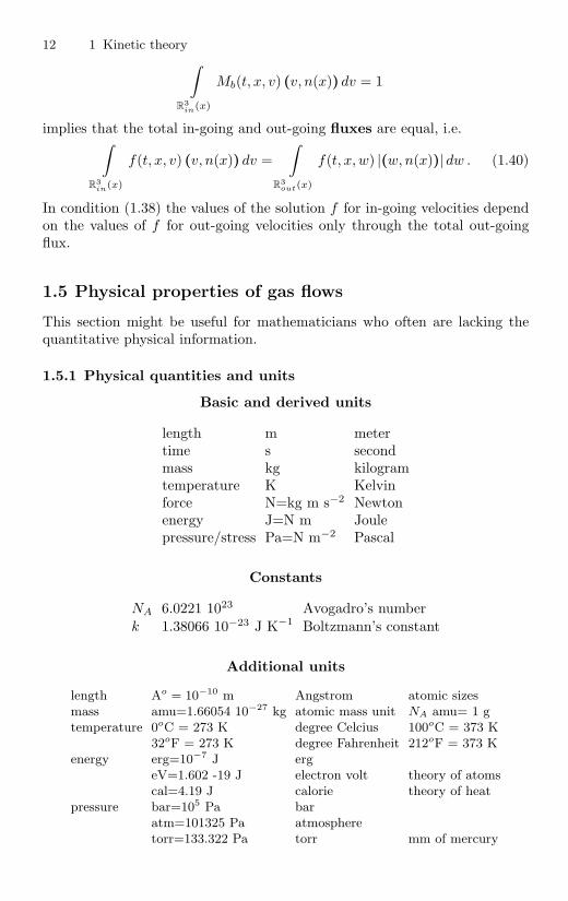
1.5.1 Physical quantities and units
Basic and derived units
length m metertime s secondmass kg kilogramtemperature K Kelvinforce N=kg m s−2 Newtonenergy J=N m Joulepressure/stress Pa=N m−2 Pascal
Constants
NA 6.0221 1023 Avogadro’s numberk 1.38066 10−23 J K−1 Boltzmann’s constant
Additional units
length Ao = 10−10 m Angstrom atomic sizesmass amu=1.66054 10−27 kg atomic mass unit NA amu= 1 gtemperature 0oC = 273 K degree Celcius 100oC = 373 K
32oF = 273 K degree Fahrenheit 212oF = 373 Kenergy erg=10−7 J erg
eV=1.602 -19 J electron volt theory of atomscal=4.19 J calorie theory of heat
pressure bar=105 Pa baratm=101325 Pa atmospheretorr=133.322 Pa torr mm of mercury
1.5 Physical properties of gas flows 13
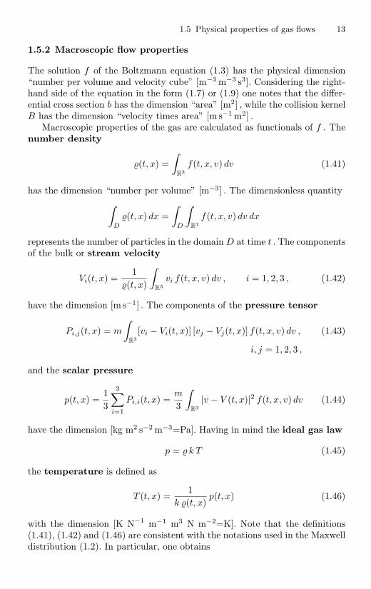
1.5.2 Macroscopic flow properties
The solution f of the Boltzmann equation (1.3) has the physical dimension“number per volume and velocity cube” [m−3 m−3 s3]. Considering the right-hand side of the equation in the form (1.7) or (1.9) one notes that the differ-ential cross section b has the dimension “area” [m2] , while the collision kernelB has the dimension “velocity times area” [m s−1 m2] .
Macroscopic properties of the gas are calculated as functionals of f . Thenumber density
(t, x) =∫
R3f(t, x, v) dv (1.41)
has the dimension “number per volume” [m−3] . The dimensionless quantity∫D
(t, x) dx =∫
D
∫R3
f(t, x, v) dv dx
represents the number of particles in the domain D at time t . The componentsof the bulk or stream velocity
Vi(t, x) =1
(t, x)
∫R3
vi f(t, x, v) dv , i = 1, 2, 3 , (1.42)
have the dimension [m s−1] . The components of the pressure tensor
Pi,j(t, x) = m
∫R3
[vi − Vi(t, x)] [vj − Vj(t, x)] f(t, x, v) dv , (1.43)
i, j = 1, 2, 3 ,
and the scalar pressure
p(t, x) =13
3∑i=1
Pi,i(t, x) =m
3
∫R3
|v − V (t, x)|2 f(t, x, v) dv (1.44)
have the dimension [kg m2 s−2 m−3=Pa]. Having in mind the ideal gas law
p = k T (1.45)
the temperature is defined as
T (t, x) =1
k (t, x)p(t, x) (1.46)
with the dimension [K N−1 m−1 m3 N m−2=K]. Note that the definitions(1.41), (1.42) and (1.46) are consistent with the notations used in the Maxwelldistribution (1.2). In particular, one obtains

14 1 Kinetic theory
m
3 k
∫R3
|v − V |2 feq(v) dv = T .
The fluxes (1.40) have the dimension “number per area and time” [m−2 s−1].The components of the heat flux vector
qi(t, x) =m
2
∫R3
[vi − Vi(t, x)] |v − V (t, x)|2 f(t, x, v) dv , (1.47)
i = 1, 2, 3 ,
have the dimension [kg m3 s−3 m−3 = J m−2 s−1] representing the transportof energy (heat) through some area per unit of time.
Further quantities of interest are the speed of sound
vsound(t, x) =
√γ k T (t, x)
m(1.48)
and the Mach number
Mach(t, x) =|V (t, x)|
vsound(t, x)(1.49)
which measures the bulk velocity in multiples of the speed of sound. Thespecific heat ratio γ used in (1.48) is related to the number β of degrees offreedom of the gas molecules as γ = (β+2)/β . Monatomic gases (like helium)have only three translational degrees of freedom so that γ = 5/3 . Diatomicmolecules (like oxygen or nitrogen) have, in addition, two rotational degreesof freedom so that γ = 7/5 .
1.5.3 Molecular flow properties
The mean molecule velocity (in equilibrium)
v =1
∫R3
|v| feq(v) dv =
√8kT
πm(1.50)
is calculated using the Maxwell distribution (1.2) with V = 0 . The meanfree path L is the average distance travelled by a molecule between collisions.Heuristically it is derived as follows. Let d be the interaction distance (e.g.the diameter in the hard sphere case). Then the interaction area is π d2 andthe average number of collisions during time t is π d2
√2 v t . The factor
√2
takes into account the relative velocity of the colliding particles. The meanfree path is obtained as
L =path length
number of collisions=
v t
π d2√
2 v t =
1√2 π d2
. (1.51)
To calculate the mean free path one needs the molecule diameter and thedensity (or pressure and temperature) of the gas.
1.5 Physical properties of gas flows 15
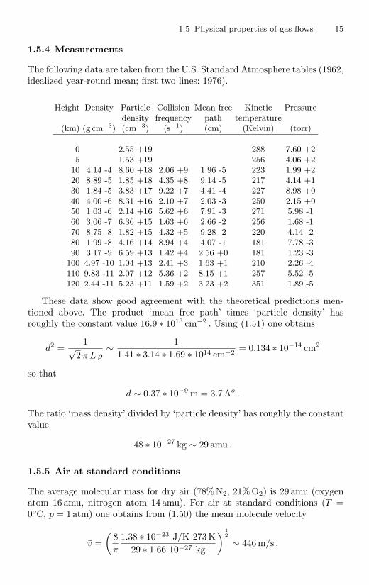
1.5.4 Measurements
The following data are taken from the U.S. Standard Atmosphere tables (1962,idealized year-round mean; first two lines: 1976).
Height Density Particle Collision Mean free Kinetic Pressuredensity frequency path temperature
(km) (g cm−3) (cm−3) (s−1) (cm) (Kelvin) (torr)
0 2.55 +19 288 7.60 +25 1.53 +19 256 4.06 +2
10 4.14 -4 8.60 +18 2.06 +9 1.96 -5 223 1.99 +220 8.89 -5 1.85 +18 4.35 +8 9.14 -5 217 4.14 +130 1.84 -5 3.83 +17 9.22 +7 4.41 -4 227 8.98 +040 4.00 -6 8.31 +16 2.10 +7 2.03 -3 250 2.15 +050 1.03 -6 2.14 +16 5.62 +6 7.91 -3 271 5.98 -160 3.06 -7 6.36 +15 1.63 +6 2.66 -2 256 1.68 -170 8.75 -8 1.82 +15 4.32 +5 9.28 -2 220 4.14 -280 1.99 -8 4.16 +14 8.94 +4 4.07 -1 181 7.78 -390 3.17 -9 6.59 +13 1.42 +4 2.56 +0 181 1.23 -3
100 4.97 -10 1.04 +13 2.41 +3 1.63 +1 210 2.26 -4110 9.83 -11 2.07 +12 5.36 +2 8.15 +1 257 5.52 -5120 2.44 -11 5.23 +11 1.59 +2 3.23 +2 351 1.89 -5
These data show good agreement with the theoretical predictions men-tioned above. The product ‘mean free path’ times ‘particle density’ hasroughly the constant value 16.9 ∗ 1013 cm−2 . Using (1.51) one obtains
d2 =1√
2 π L∼ 1
1.41 ∗ 3.14 ∗ 1.69 ∗ 1014 cm−2= 0.134 ∗ 10−14 cm2
so that
d ∼ 0.37 ∗ 10−9 m = 3.7Ao .
The ratio ‘mass density’ divided by ‘particle density’ has roughly the constantvalue
48 ∗ 10−27 kg ∼ 29 amu .
1.5.5 Air at standard conditions
The average molecular mass for dry air (78%N2, 21%O2) is 29 amu (oxygenatom 16 amu, nitrogen atom 14 amu). For air at standard conditions (T =0oC, p = 1atm) one obtains from (1.50) the mean molecule velocity
v =(
8π
1.38 ∗ 10−23 J/K 273K29 ∗ 1.66 10−27 kg
) 12
∼ 446m/s .

16 1 Kinetic theory
Assuming d = 3.7Ao and using (1.45), one obtains from (1.51) the mean freepath
L =1.38 ∗ 10−23 J/K 273K√
2 π ∗ 13.7 ∗ 10−20 m2 1.01 ∗ 105 N/m2∼ 61 nm .
Correspondingly, a molecule suffers about 7 ∗ 109 collisions per second. Theratio between mean free path and diameter is L/d ∼ 165 . The relative volumeoccupied by gas molecules is
π
6d3 p
k T=
π
6(0.37)3 ∗ 10−27 m3 1.01 ∗ 105 N/m2
1.38 ∗ 10−23 J/K 273K∼ 0.0007 .
The speed of sound (1.48) is
(1.4 ∗ 1.38 ∗ 10−23 J/K 273K
29 ∗ 1.66 10−27 kg
) 12
∼ 331m/s .
1.6 Properties of the collision integral
To study the collision integral (1.9), we introduce the notation
Q(f, g)(v) =12
∫R3
dw
∫S2
deB(v, w, e) ×[f(v′) g(w′) + g(v′) f(w′) − f(v) g(w) − g(v) f(w)
],
where f, g are appropriate functions on R3 and v′, w′ are defined in (1.6).
Theorem 1.9. All strictly positive integrable solutions g of the equation
Q(g, g) = 0 (1.52)
are Maxwell distributions, i.e.
g(v) = MV,T (v) , ∀v ∈ R3 , (1.53)
for some , T > 0 and V ∈ R3 .
The proof is prepared by several lemmas.
Lemma 1.10. Let v′, w′ be defined by the collision transformation (1.6). Then∫R3
∫R3
∫S2
Φ(|v − w|, (v − w, e), v, w, v′, w′) de dw dv = (1.54)∫R3
∫R3
∫S2
Φ(|v − w|, (v − w, e), v′, w′, v, w) de dw dv ,
for any appropriate test function Φ .
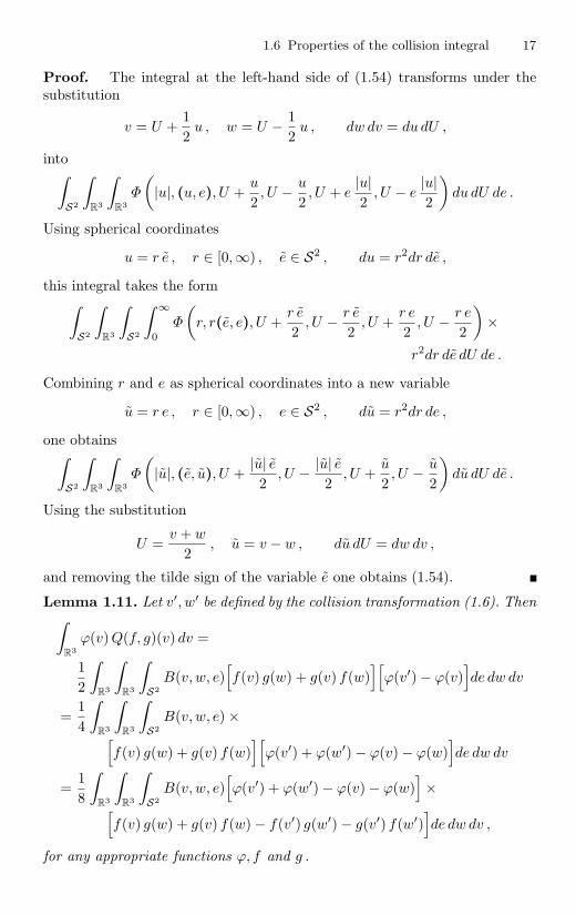
1.6 Properties of the collision integral 17
Proof. The integral at the left-hand side of (1.54) transforms under thesubstitution
v = U +12
u , w = U − 12
u , dw dv = du dU ,
into∫S2
∫R3
∫R3
Φ
(|u|, (u, e), U +
u
2, U − u
2, U + e
|u|2
, U − e|u|2
)du dU de .
Using spherical coordinates
u = r e , r ∈ [0,∞) , e ∈ S2 , du = r2dr de ,
this integral takes the form∫S2
∫R3
∫S2
∫ ∞
0
Φ
(r, r(e, e), U +
r e
2, U − r e
2, U +
r e
2, U − r e
2
)×
r2dr de dU de .
Combining r and e as spherical coordinates into a new variable
u = r e , r ∈ [0,∞) , e ∈ S2 , du = r2dr de ,
one obtains∫S2
∫R3
∫R3
Φ
(|u|, (e, u), U +
|u| e2
, U − |u| e2
, U +u
2, U − u
2
)du dU de .
Using the substitution
U =v + w
2, u = v − w , du dU = dw dv ,
and removing the tilde sign of the variable e one obtains (1.54).
Lemma 1.11. Let v′, w′ be defined by the collision transformation (1.6). Then∫R3
ϕ(v)Q(f, g)(v) dv =
12
∫R3
∫R3
∫S2
B(v, w, e)[f(v) g(w) + g(v) f(w)
][ϕ(v′) − ϕ(v)
]de dw dv
=14
∫R3
∫R3
∫S2
B(v, w, e) ×[f(v) g(w) + g(v) f(w)
][ϕ(v′) + ϕ(w′) − ϕ(v) − ϕ(w)
]de dw dv
=18
∫R3
∫R3
∫S2
B(v, w, e)[ϕ(v′) + ϕ(w′) − ϕ(v) − ϕ(w)
]×[
f(v) g(w) + g(v) f(w) − f(v′) g(w′) − g(v′) f(w′)]de dw dv ,
for any appropriate functions ϕ, f and g .
18 1 Kinetic theory
Proof. Note that B depends on its arguments via |v − w| and (v − w, e) ,according to (1.10). Thus, Lemma 1.10 implies the first part of the assertion.Changing the variables v and w , using the substitution e = −e , de = deand removing the tilde sign over e leads to∫
R3ϕ(v)Q(f, g)(v) dv =
12
∫R3
∫R3
∫S2
B(w, v,−e)× (1.55)[f(v) g(w) + g(v) f(w)
][ϕ(v′(w, v,−e)) − ϕ(w)
]de dv dw .
Using the first part of the assertion, (1.55) and the property
B(w, v,−e) = B(v, w, e) ,
one obtains the second part of the assertion, and one more application ofLemma 1.10 gives the third part.
A function ψ : R3 → R is called collision invariant if
ψ(v′) + ψ(w′) = ψ(v) + ψ(w) , ∀ v, w ∈ R3 , e ∈ S2 . (1.56)
It follows from conservation of mass, momentum and energy during collisionsthat the functions
ψ0(v) = 1 , ψj(v) = vj , j = 1, 2, 3 , ψ4(v) = |v|2 (1.57)
are collision invariants. Note that Lemma 1.11 implies∫R3
ψ(v)Q(g, g)(v) dv = 0 , (1.58)
for any collision invariant ψ , independently of the particular choice of thefunction g .
Lemma 1.12. A continuous function ψ : R3 → R is a collision invariant if
and only if it is a linear combination of the basic collision invariants (1.57),i.e.
ψ(v) = a + (b, v) + c |v|2 , for some a, c ∈ R , b ∈ R3 .
Proof of Theorem 1.9. Assuming that the function g is strictly positiveone can use log g as a test function. It follows from Lemma 1.11 that∫
R3log g(v)Q(g, g)(v) dv = (1.59)
−14
∫R3
∫R3
∫S2
B(v, w, e) g(v) g(w)[g(v′) g(w′)g(v) g(w)
− 1]
logg(v′) g(w′)g(v) g(w)
dw dv de .
Since the expression (z − 1) log z is always non-negative and vanishes only ifz = 1 , one obtains from (1.59) Boltzmann’s inequality

1.6 Properties of the collision integral 19∫R3
log g(v)Q(g, g)(v) dv ≤ 0 (1.60)
and concludes that ∫R3
log g(v)Q(g, g)(v) dv = 0 (1.61)
if and only if
g(v′) g(w′) = g(v) g(w) , ∀ v, w ∈ R3 , e ∈ S2 ,
i.e., if the function log g is a collision invariant (cf. (1.56)). Thus, accordingto Lemma 1.12, property (1.61) is fulfilled if and only if the function g is ofthe form
g(v) = exp(a + (b, v) + c |v|2
), for some a, c ∈ R , b ∈ R
3 .
Note that c must be negative so that g is integrable over the velocity space.Thus, the function g takes the form (1.53).
Let f(t, v) be a solution of the spatially homogeneous Boltzmannequation
∂
∂tf(t, v) = Q(f, f)(t, v) . (1.62)
Note that (1.58) implies
d
dt
∫R3
ψj(v) f(t, v) dv = 0 , (1.63)
for the basic collision invariants (1.57). The functional
H[f ](t) =∫
R3log f(t, v) f(t, v) dv (1.64)
is called H-functional. Using (1.62) and (1.63) (with j = 0) one obtains theequation
d
dtH[f ](t) =
∫R3
log f(t, v)Q(f, f)(t, v) dv .
Thus, according to (1.60), the H-functional is a monotonically decreasing func-tion in time, unless f has the form (1.53) with constant parameters , V andT . In this case the H-functional has a constant value
H[f ](t) =
(log
(2π T )3/2− 3
2
), t ≥ 0 . (1.65)

20 1 Kinetic theory
Example 1.13. Let us consider the initial value problem for the spatially ho-mogeneous Boltzmann equation (1.62) with initial condition
f(0, v) = α MV,T1(v) + (1 − α)MV,T2(v) for some α ∈ [0, 1] .
The asymptotic distribution function is
limt→∞ f(t, v) = MV,T (v) with T = α T1 + (1 − α)T2 .
According to (1.65), the asymptotic value of the H-functional is
H[MV,T ] = −32
[log(2πT ) + 1
].
Fig. 1.2 shows the time evolution of the H-functional (1.64) for the hard spheremodel
B(v, w, e) =14π
|v − w|
and for the parameters
α = 0.25 , V = (0, 0, 0) , T1 = 0.1 , T2 = 0.3 , T = 0.25 .
The solid line in this figure represents the H-functional, while the dotted lineshows its asymptotic value 3/2 [log(2/π) − 1] ∼ −2.1774 .
0 1 2 3 4 5-2.1775
-2.175
-2.1725
-2.17
-2.1675
-2.165
-2.1625
Fig. 1.2. Time evolution of the H-functional

1.7 Moment equations 21
1.7 Moment equations
Here we use the property (1.58) of the collision integral. Multiplying the Boltz-mann equation (1.3) by one of the basic collision invariants (1.57), integratingthe result with respect to v over the velocity space and changing the order ofintegration and differentiation, one obtains the equations
∂
∂t
∫R3
ψj(v)f(t, x, v) dv +3∑
i=1
∂
∂xi
∫R3
vi ψj(v)f(t, x, v) dv = 0 , (1.66)
j = 0, 1, 2, 3, 4 .
Using the definition (1.41) of the number density and the notations
li(t, x) =∫
R3vi f(t, x, v) dv , i = 1, 2, 3 ,
Li,j(t, x) =∫
R3vi vj f(t, x, v) dv , i, j = 1, 2, 3 ,
and
ri(t, x) =∫
R3vi |v|2 f(t, x, v) dv , i = 1, 2, 3 ,
we rewrite equations (1.66) in terms of moments of the distribution function
∂
∂t(t, x) +
3∑i=1
∂
∂xili(t, x) = 0 ,
∂
∂tlj(t, x) +
3∑i=1
∂
∂xiLi,j(t, x) = 0 , j = 1, 2, 3 , (1.67)
∂
∂t
3∑i=1
Li,i(t, x) +3∑
i=1
∂
∂xiri(t, x) = 0 .
Recalling the definitions (1.42)-(1.44), (1.46) and (1.47), one obtains
Vi(t, x) =1
(t, x)li(t, x) ,
Pi,j(t, x) = m[Li,j(t, x) − (t, x)Vi(t, x)Vj(t, x)
],
(t, x) k T (t, x) =m
3
[3∑
i=1
Li,i(t, x) − (t, x) |V (t, x)|2]
and
22 1 Kinetic theory
qi(t, x) =
m
2
⎡⎣ri − 2
3∑j=1
Vj Li,j + li |V |2 − Vi
3∑j=1
Lj,j + 2Vi
3∑j=1
Vj lj − Vi |V |2
⎤⎦
=m
2
⎡⎣ri − 2
3∑j=1
Vj Li,j − Vi
3∑j=1
Lj,j + 2 Vi |V |2⎤⎦
=m
2ri −
3∑j=1
Vj Pi,j −3 k
2Vi T − m
2 Vi |V |2 ,
for i, j = 1, 2, 3 . Thus, the system of equations (1.67) implies
∂
∂t(t, x) +
3∑i=1
∂
∂xi
[Vi(t, x) (t, x)
]= 0 , (1.68)
∂
∂t
[(t, x)Vj(t, x)
]+ (1.69)
3∑i=1
∂
∂xi
[Vi(t, x) (t, x)Vj(t, x)
]= − 1
m
3∑i=1
∂
∂xiPi,j(t, x) , j = 1, 2, 3 ,
and
∂
∂t
[3 k
2m(t, x)T (t, x) +
12
(t, x) |V (t, x)|2]
+ (1.70)
3∑i=1
∂
∂xi
[Vi(t, x)
(3 k
2m(t, x)T (t, x) +
12
(t, x) |V (t, x)|2)]
=
− 1m
3∑i=1
∂
∂xi
⎡⎣qi(t, x) +
3∑j=1
Pi,j(t, x)Vj(t, x)
⎤⎦ .
Equation (1.68) transforms into
∂
∂t(t, x) + (V (t, x),∇x) (t, x) + (t, x) div V (t, x) = 0 . (1.71)
Using (1.68), the left-hand side of equation (1.69) transforms into
∂
∂t
[(t, x)
]Vj(t, x) + (t, x)
∂
∂t
[Vj(t, x)
]+
3∑i=1
∂
∂xi
[Vi(t, x) (t, x)
]Vj(t, x) +
3∑i=1
Vi(t, x) (t, x)∂
∂xi
[Vj(t, x)
]
= (t, x)[
∂
∂tVj(t, x) + (V (t, x),∇x)Vj(t, x)
]

1.7 Moment equations 23
so that equation (1.69) takes the form
∂
∂tVj(t, x) + (V (t, x),∇x)Vj(t, x) = − 1
m(t, x)
3∑i=1
∂
∂xiPi,j(t, x) ,
j = 1, 2, 3 . (1.72)
The two parts of the left-hand side of equation (1.70) transform into
∂
∂t
[(t, x)
]T (t, x) + (t, x)
∂
∂t
[T (t, x)
]+
3∑i=1
∂
∂xi
[Vi(t, x)(t, x)
]T (t, x) +
3∑i=1
Vi(t, x) (t, x)∂
∂xi
[T (t, x)
]
= (t, x)[
∂
∂tT (t, x) + (V (t, x),∇x)T (t, x)
]
and
12
(3∑
j=1
∂
∂t
[(t, x)Vj(t, x)
]Vj(t, x) +
3∑j=1
(t, x)Vj(t, x)∂
∂t
[Vj(t, x)
]+
3∑i=1
3∑j=1
∂
∂xi
[Vi(t, x) (t, x)Vj(t, x)
]Vj(t, x) +
3∑i=1
3∑j=1
Vi(t, x) (t, x)Vj(t, x)∂
∂xi
[Vj(t, x)
])
=12
3∑j=1
Vj(t, x)
[− 1
m
3∑i=1
∂
∂xiPi,j(t, x)
]+
12
3∑j=1
(t, x)Vj(t, x)
[− 1
m(t, x)
3∑i=1
∂
∂xiPi,j(t, x)
]
= − 1m
3∑j=1
Vj(t, x)3∑
i=1
∂
∂xiPi,j(t, x)
so that equation (1.70) takes the form
∂
∂tT (t, x) + (V (t, x),∇x)T (t, x) = (1.73)
− 23k (t, x)
⎛⎝div q(t, x) +
3∑i,j=1
Pi,j(t, x)∂
∂xiVj(t, x)
⎞⎠ .
The system (1.71), (1.72), (1.73) contains five equations for 13 unknown func-tions , V, P and q . Note that the symmetric matrix P is defined by its uppertriangle.
24 1 Kinetic theory
If the distribution function is a Maxwellian, i.e.
f(t, x, v) = (t, x)[
m
2π k T (t, x)
] 32
exp(−m |v − V (t, x)|2
2 k T (t, x)
),
then one obtains
Pi,j(t, x) = p(t, x) δi,j , qi(t, x) = 0 , i, j = 1, 2, 3 . (1.74)
Assuming that the gas under consideration is close to equilibrium, i.e. itsdistribution function is close to a Maxwellian, property (1.74) can be usedas a closure relation. Then the number of unknown functions reduces to five.These functions are the density , the stream velocity V and the temperatureT (or, equivalently, the pressure p). Equations (1.71), (1.72) and (1.73) reduceto the Euler equations
∂
∂t(t, x) + (V (t, x),∇x) (t, x) + (t, x) div V (t, x) = 0 ,
∂
∂tVj(t, x) + (V (t, x),∇x)Vj(t, x) +
k
m(t, x)∂
∂xj
[(t, x)T (t, x)
]= 0 ,
j = 1, 2, 3 ,
and
∂
∂tT (t, x) + (V (t, x),∇x)T (t, x) +
23
T (t, x) divV (t, x) = 0 .
They describe a so-called Euler (or ideal) fluid.Besides (1.74), other closure relations (also called constitutive equations)
are used. If one assumes
Pi,j(t, x) = p(t, x) δi,j − µ
[∂
∂xiVj(t, x) +
∂
∂xjVi(t, x)
]− λ δi,j divV (t, x) ,
qi(t, x) = −κ∂
∂xiT (t, x) , i, j = 1, 2, 3 ,
then equations (1.71)-(1.73) reduce to the Navier-Stokes equations. Theydescribe a so-called Navier-Stokes-Fourier (or viscous and thermally conduct-ing) fluid. Here µ, λ are the viscosity coefficients and κ is the heat conductioncoefficient. All these coefficients can be functions of the density and thetemperature T .
1.8 Criterion of local equilibrium
If the distribution function f is close to a Maxwell distribution, then one canexpect that the description of the flow by the Boltzmann equation is close

1.8 Criterion of local equilibrium 25
to its description by the system of Euler equations. The numerical solutionof the Boltzmann equation is, in general, much more complicated than thenumerical solution of the Euler equations, because the distribution functiondepends on seven variables. In contrast, the system of Euler equations containsfive unknown functions depending on four variables. Therefore it makes senseto divide the domain D into two subdomains with the kinetic descriptionof the flow by the Boltzmann equation in the first subdomain and with thehydrodynamic description by the Euler equations in the second subdomain.
In this section we derive a functional that indicates the deviation of thedistribution function f from a Maxwell distribution with the same density,stream velocity and temperature. In the derivation we skip the arguments t, xwhich are assumed to be fixed. Note that (cf. (1.2))
feq(v) = ( m
k T
) 32
M0,1
(v − V√kT/m
).
In analogy we first introduce the normalized function
f(v) =1
(k T
m
) 32
f(V + v
√k T/m
)(1.75)
and study its deviation from M0,1 . The general case is then found by anappropriate rescaling.
We consider a function
ψ(v) = a + (b, v) + (C v, v) + (d, v) |v|2 + e |v|4 , (1.76)
where the parameters a, e ∈ R , b, d ∈ R3 , C ∈ R
3×3 are chosen in such away that ∫
R3ϕ(v)M0,1(v)
[1 + ψ(v)
]dv =
∫R3
ϕ(v) f(v) dv , (1.77)
for the test functions
ϕ(v) = 1 , vi , vi vj , vi |v|2 , |v|4 , i, j = 1, 2, 3 .
Note that there are 14 equations and 14 unknown variables. The weightedL2-norm of the function (1.76)
(∫R3
ψ(v)2 M0,1(v) dv
) 12
(1.78)
will be used as a measure of deviation from local equilibrium.Conditions (1.77) are transformed into

26 1 Kinetic theory ∫R3
ψ(v)M0,1(v) dv = 0 , (1.79a)∫R3
vi ψ(v)M0,1(v) dv = 0 , (1.79b)∫R3
vi vj ψ(v)M0,1(v) dv = τi,j , (1.79c)∫R3
vi |v|2 ψ(v)M0,1(v) dv = 2 qi , (1.79d)∫R3
|v|4 ψ(v)M0,1(v) dv = γ , (1.79e)
where the notations
τi,j =∫
R3vi vj f(v) dv − δi,j , (1.80)
qi =12
∫R3
vi |v|2 f(v) dv (1.81)
and (cf. (A.5))
γ =∫
R3|v|4 f(v) dv − 15 (1.82)
are used. Note that∫R3
f(v) dv = 1 ,
∫R3
v f(v) dv = 0 ,
∫R3
|v|2 f(v) dv = 3 . (1.83)
Using Lemma A.1, all integrals in (1.79a)-(1.79e) can be computed so thatone obtains a system of equations for the parameters a, b, C, d and e
a + tr C + 15 e = 0 , (1.84a)bi + 5 di = 0 , (1.84b)
a δi,j + 2Ci,j + tr C δi,j + 35 e δi,j = τi,j , (1.84c)5 bi + 35 di = 2 qi , (1.84d)
15 a + 35 tr C + 945 e = γ , (1.84e)
where i, j = 1, 2, 3 . Note that
3∑k,l=1
Ck,l
∫R3
vi vj vk vl M0,1(v) dv = 2Ci,j if i = j
and
1.8 Criterion of local equilibrium 27
3∑k,l=1
Ck,l
∫R3
v2i vk vl M0,1(v) dv =
3∑k=1
Ck,k
∫R3
v2i v2
k M0,1(v) dv =3∑
k=1
Ck,k + 2Ci,i if i = j .
From (1.84b) and (1.84d) we immediately obtain
bi = −qi , di =15
qi , i = 1, 2, 3 . (1.85)
Taking trace of the matrices in equation (1.84c) and using tr τ = 0 (cf. (1.83)),we obtain a linear system for the scalar parameters a, tr C and e ,⎛
⎝ 1 1 153 5 10515 35 945
⎞⎠⎛⎝ a
tr Ce
⎞⎠ =
⎛⎝ 0
0γ
⎞⎠ .
Thus these parameters are
a =18
γ , tr C = −14
γ , e =1
120γ . (1.86)
Using the equation (1.84c) we get
Ci,j =12
τi,j −γ
12δi,j , i, j = 1, 2, 3 . (1.87)
The function (1.76) is now entirely defined by (1.85)-(1.87).According to (1.79a)-(1.79e) one obtains (cf. (1.78))
∫R3
ψ(v)2 M0,1(v) dv =3∑
i,j=1
Ci,j τi,j + 23∑
i=1
di qi + e γ
=12
3∑i,j=1
τ2i,j −
γ
12
3∑i=1
τi,i +25
3∑i=1
q2i +
1120
γ2
=12||τ ||2F +
25|q|2 +
1120
γ2 , (1.88)
where
||A||F =
√√√√ 3∑i,j=1
a2i,j (1.89)
denotes the Frobenius norm of a matrix A .Finally we express the auxiliary quantities (1.80)-(1.82) through the stan-
dard macroscopic quantities (defined by the function f). Using (1.75) oneobtains

28 1 Kinetic theory
τi,j =1
(k T
m
) 32∫
R3vi vj f
(V + v
√k T/m
)dv − δi,j
=1
m
k T
∫R3
(vi − Vi) (vj − Vj) f(v) dv − δi,j =1
k T
[Pi,j − p δi,j
],
qi =1
(k T
m
) 32 1
2
∫R3
vi |v|2 f(V + v
√k T/m
)dv
=1
( m
k T
) 32 1
2
∫R3
(vi − Vi) |v − V |2 f(v) dv =1
k T
( m
k T
) 12
qi
and
γ =1
(k T
m
) 32∫
R3|v|4 f
(V + v
√k T/m
)dv − 15
=1
( m
k T
)2 ∫R3
|v − V |4 f(v) dv − 15 =1
( m
k T
)2γ ,
where
γ = γ(t, x) =∫
R3|v − V (t, x)|4 f(t, x, v) dv − 15 (t, x)
(k T (t, x)
m
)2
. (1.90)
Thus, according to (1.88), the quantity (1.78) takes the form (cf. (1.89))
Crit(t, x) =1
k T
(12||P − p I||2F +
2m
5 k T|q|2 +
m4
120 k2 T 2γ2
)1/2
. (1.91)
The dimensionless function (1.91) will be used as a criterion of local equilib-rium.
1.9 Scaling transformations
For different purposes it is reasonable to use some scaling for the Boltzmannequation in order to work with dimensionless variables and functions. Let
0 > 0 , V0 > 0 , X0 > 0 , t0 =X0
V0
be the typical density, speed, length and time of the problem. According to(1.50), the typical speed is proportional to the square root of the typicaltemperature T0 , e.g., V0 =
√k T0/m . Consider the dimensionless variables
t =t
t0, x =
x
X0, v =
v
V0
and introduce the dimensionless function

1.9 Scaling transformations 29
f(t, x, v) = c f(t, x, v) , c = V 30 −1
0 ,
where 0 is the typical density (number per volume). One obtains
∂
∂tf(t, x, v) =
1c t0
∂
∂tf(t, x, v) ,
(v,∇x) f(t, x, v) =V0
c X0(v,∇x) f(t, x, v) =
1c t0
(v,∇x) f(t, x, v)
and∫R3
∫S2
B(v, w, e)×[f(t, x, v′(v, w, e)) f(t, x, w′(v, w, e)) − f(t, x, v) f(t, x, w)
]de dw
=V 3
0
c2
∫R3
∫S2
B(v, w, e)[f(t, x, V −1
0 v′(v, w, e)) f(t, x, V −10 w′(v, w, e)) −
f(t, x, V −10 v) f(t, x, V −1
0 w)]de dw
=V 3
0
c2
∫R3
∫S2
B(v, w, e) ×[f(t, x, v′(v, w, e)) f(t, x, w′(v, w, e)) − f(t, x, v) f(t, x, w)
]de dw .
Thus, the new function satisfies
∂
∂tf(t, x, v) + (v,∇x) f(t, x, v) = t0 0
∫R3
∫S2
B(V0 v, V0 w, e)× (1.92)[f(t, x, v′(v, w, e)) f(t, x, w′(v, w, e)) − f(t, x, v) f(t, x, w)
]de dw .
Using the form (1.10) one obtains
B(V0 v, V0 w, e) = V0 |v − w| b(V0 |v − w|, θ)sin θ
, θ = arccos(v − w, e)|v − w| .
Taking into account the definition of the equilibrium mean free path (cf.(1.51))
L0 =1√
2 π d2 0
and of the Knudsen number
Kn =L0
X0, (1.93)
equation (1.92) is transformed into

30 1 Kinetic theory
∂
∂tf(t, x, v) + (v,∇x) f(t, x, v) =
1Kn
∫R3
∫S2
B(v, w, e)× (1.94)[f(t, x, v′(v, w, e)) f(t, x, w′(v, w, e)) − f(t, x, v) f(t, x, w)
]de dw .
where the collision kernel has the form
B(v, w, e) =|v − w|√
2 π d2
b(|v − w|, θ)sin θ
, θ = arccos(v − w, e)|v − w| ,
with
b(|v − w|, θ) = b(V0 |v − w|, θ) .
Note that B is dimensionless.In the hard sphere case the scaled Boltzmann equation (1.94) takes
the form (cf. (1.28))
∂
∂tf(t, x, v) + (v,∇x) f(t, x, v) = (1.95)
14√
2π Kn
∫R3
∫S2
|v − w|[f(t, x, v′) f(t, x, w′) − f(t, x, v) f(t, x, w)
]de dw ,
where v′, w′ are defined in (1.6), or (cf. (1.18))
∂
∂tf(t, x, v) + (v,∇x) f(t, x, v) =
12√
2π Kn×∫
R3
∫S2
|(e, v − w)|[f(t, x, v∗) f(t, x, w∗) − f(t, x, v) f(t, x, w)
]de dw ,
where v∗ and w∗ are defined in (1.12).
1.10 Comments and bibliographic remarks
Section 1.1
The Boltzmann equation (1.3) first appeared in [36]. The history of kinetictheory and, in particular, of Boltzmann’s contributions is described in [49].
Section 1.2
Fig. 1.1 has been adapted from [82]. Both collision transformations (1.6) and(1.12) are used in the literature. Though equivalent, one of them may bepreferable in a certain context. As we will see later, (1.6) is slightly moreconvenient for numerical purposes, since the corresponding distribution ofthe direction vector e is uniform (cf. (1.29)), while depending on the relativevelocity (cf. (1.30)) in the case of (1.12).

1.10 Comments and bibliographic remarks 31
Section 1.3
A discussion of soft and hard interactions can be found, for example, in [60]and [48, Sect. 2.4, 2.5]. The notion of “Maxwell molecules” refers to a paperby Maxwell in 1866, according to [48, p.71]. The variable diameter hard spheremodel was introduced in [23] in order to correct the non-realistic temperaturedependence of the viscosity coefficient in the hard sphere model, while keepingits main advantages such as the finite total cross-section and the isotropicscattering. There are further models for collision kernels and differential cross-sections in the literature, e.g., in [25], [78], [113], [114].
Section 1.4
First studies of boundary conditions for the Boltzmann equation go back toMaxwell 1879 (cf. [48, p.118, Ref. 11]). Concerning a more detailed discussionof boundary conditions we refer to [51, Ch. 8], [48, Ch. III], [25, Sect. 4.5]. Arather intuitive interpretation of boundary conditions will be given in Chap-ter 2 on the basis of stochastic models.
Section 1.5
The measurement data were taken from [131] and [40]. Concerning the meanfree path, the following simple argument is given in [48, p.19]: On averagethere is only one other molecule in the cylinder of base π d2 and height L sothat π d2 L ∼ 1 and L ∼ 1/( π d2) . Formula (1.51) has been taken from[25, p.91]. Note that L >> d is an assumption for the validity of the equation.Concerning the speed of sound, we refer to [48, p.233] and [25, pp.25, 64, 82,165].
Section 1.6
The first discussion on collision invariants is due to Boltzmann himself. Laterthe problem was addressed by many authors. The corresponding referencesand a proof of Lemma 1.12 are given in [51, p.36]. In the non-homogeneous casethe situation with the H-functional is more complicated. The correspondingdiscussion can be found in [51, p.51]. The curve in Fig. 1.2 was obtained in[100] using a conservative deterministic scheme for the Boltzmann equationand an adaptive trapezoid quadrature for the integral (1.64).
Section 1.7
Concerning closure relations we refer to [48, p.85]. Note the remark from [25,p.186]: “from the kinetic theory point of view, both the Euler and Navier-Stokes equations may be regarded as ‘five moment’ solutions of the Boltzmannequation, the former being valid for the Kn → 0 limit and the latter forKn << 1 .”
32 1 Kinetic theory
Section 1.8
The problem of detecting local equilibrium using some macroscopic quantitieswas discussed by several authors. In [123] the quantity (criterion)
Crit(t, x) =c
T (t, x)||P (t, x) − p(t, x) I||F
was derived on the basis of physical intuition. In [135], [38] the heat flux basedcriterion
Crit(t, x) =c
T (t, x)3/2|q(t, x)|
was used. Here c > 0 denotes some constant. Note that the functional (1.91)uses only moments of the function f so that it can be computed using stochas-tic numerics. The question how to decide where the hydrodynamic descriptionis sufficient and how to couple the numerical procedures for the Boltzmannand Euler equations was investigated by a number of authors [37], [74], [101],[103], [117], [102], [199], [200], [201], [168].
Section 1.9
The dimensionless Knudsen number (cf. [107]) defined in (1.93) describes thedegree of rarefaction of a gas. For small Knudsen numbers the collisions be-tween particles become dominating.
2
Related Markov processes
2.1 Boltzmann type piecewise-deterministic Markovprocesses
A piecewise-deterministic Markov process is a jump process that changes itsstate in a deterministic way between jumps. Here we introduce a class ofpiecewise-deterministic Markov processes related to Boltzmann type equa-tions. The processes describe the behavior of a system of particles. Eachparticle is characterized by its position, velocity and weight. The numberof particles in the system is variable.
2.1.1 Free flow and state space
Consider the system of ordinary differential equations
d
dtx(t) = v(t) ,
d
dtv(t) = E(x(t)) , t ≥ 0 , (2.1)
with initial condition
x(0) = x , v(0) = v , x, v ∈ R3 . (2.2)
Assume the force term E is globally Lipschitz continuous so that no explosionoccurs. The unique solution X(t, x, v), V (t, x, v) of (2.1), (2.2) is called freeflow and determines the behavior of the particles between jumps. In thespecial case E = 0 one obtains
X(t, x, v) = x + t v , V (t, x, v) = v , t ≥ 0 .
Note that t, x and v are dimensionless variables.We first define the state space of a single particle. Denote by
∂in
(D × R
3)
= (2.3){(x, v) ∈ ∂D × R
3 : X(s, x, v) ∈ D , ∀s ∈ (0, t) , for some t > 0}
34 2 Related Markov processes
the part of the boundary from which the free flow goes inside the domain D ,and by
∂out
(D × R
3)
= (2.4){(x, v) ∈ ∂D × R
3 : X(−s, x, v) ∈ D , ∀s ∈ (0, t) , for some t > 0}
the part of the boundary at which the free flow goes outside the domain. Thestate space of a single particle is
E1 = E1 × (0,∞) , (2.5)
where
E1 =(D × R
3)∪(∂in
(D × R
3)\ ∂out
(D × R
3) )
. (2.6)
It is the open set D × R3 × (0,∞) extended by some part of its boundary,
which is characterized by the free flow.The state space of the process is
E =∞⋃
ν=1
(E1)ν ∪ {(0)} .
Elements of E are denoted by
z = (ν, ζ) : ν = 1, 2, . . . , ζ = (x1, v1, g1; . . . ;xν , vν , gν) , (2.7)
and (0) is the zero-state of the system. Define a metric on E in such a waythat
limn→∞ ((νn, ζn), (ν, ζ)) = 0 ⇐⇒
∃ l : νn = ν , ∀n ≥ l and limk→∞
ζl+k = ζ in R7ν .
2.1.2 Construction of sample paths
For z = (ν, ζ) ∈ E (cf. (2.7)) define the exit time
t∗(z) = min1≤i≤ν
t∗(xi, vi) , (2.8)
where (cf. (2.6))
t∗(x, v) ={
inf {t > 0 : X(t, x, v) ∈ ∂D} ,∞ , if no such time exists ,
for (x, v) ∈ E1 .
Introduce the set of exit states
Γ ={
(ν, ζ) : ζ = Xν(t∗(ν, ζ ′), ζ ′) , for some (ν, ζ ′) ∈ E}
, (2.9)

2.1 Boltzmann type piecewise-deterministic Markov processes 35
where
(2.10)
Xν(t, ζ) =(X(t, x1, v1), V (t, x1, v1), g1; . . . ;X(t, xν , vν), V (t, xν , vν), gν
).
Consider a kernel Q mapping E into M(E) , a rate function
λ(z) = Q(z,E) , (2.11)
and a kernel Qref mapping Γ into the set of probability measures on (E,B(E)) .Starting at z , the particles move according to the free flow,
Z(t) = Xν(t, ζ) , t < τ1 . (2.12)
The random jump time τ1 satisfies (cf. (2.8))
Prob(τ1 > t) = χ[0,t∗(z))(t) exp(−∫ t
0
λ(ν,Xν(s, ζ)) ds
), t ≥ 0 . (2.13)
Note that τ1 ≤ t∗(z) and
Prob(τ1 = t∗(z)) = exp
(−∫ t∗(z)
0
λ(ν,Xν(s, ζ)) ds
).
At time τ1 the process jumps into a state z1 . This state is distributed accord-ing to the transition measure{
λ(z)−1Q(z, dz1) , if τ1 < t∗(z) ,Qref(z, dz1) , if τ1 = t∗(z) ,
(2.14)
where z = Xν(τ1, ζ) . Then the construction is repeated with z1 replacing z ,and τ2 replacing τ1 .
It is assumed that, for every z ∈ E , the mean number of jumps on finitetime intervals is finite, i.e.
E
∞∑k=1
χ[0,S](τk) < ∞ , ∀S ≥ 0 . (2.15)
2.1.3 Jump behavior
The system performs jumps of two different types, corresponding to the casesz ∈ E and z ∈ Γ in (2.14).
Jumps of type A occur while the system is in the state space and would staythere for a non-zero time interval. These (un-enforced) jumps are generatedby the rate function (2.11). Examples are
• collisions of particles (type A1),

36 2 Related Markov processes
• scattering of particles (type A2),• death (annihilation, absorption) of particles (type A3),• birth (creation) of new particles (type A4).
Jumps of type B occur when the system is about to leave the state space.These (enforced) jumps are caused by the free flow hitting the boundary.Examples are
• reflection of particles at the boundary,• absorption (outflow) of particles at the boundary.
Jumps of type A
We consider a kernel of the form
Q(z; dz) = Qcoll(z; dz) + Qscat(z; dz) + Q−(z; dz) + Q+(z; dz) , (2.16)
where z ∈ E (cf. (2.7)). We describe the jumps by some deterministic trans-formation depending on random parameters.
A1: Collisions of particles
The basic jump transformation is
[Jcoll(z; i, j, θ)]k =
⎧⎪⎪⎪⎪⎨⎪⎪⎪⎪⎩
(xk, vk, gk) , if k ≤ ν , k = i, j ,(xcoll, vcoll, γcoll(z; i, j, θ)) , if k = i ,(ycoll, wcoll, γcoll(z; i, j, θ)) , if k = j ,(xi, vi, gi − γcoll(z; i, j, θ)) , if k = ν + 1 ,(xj , vj , gj − γcoll(z; i, j, θ)), if k = ν + 2 ,
(2.17)
where θ belongs to some parameter set Θcoll , and the functions xcoll, vcoll,ycoll, wcoll depend on the arguments (xi, vi, xj , vj , θ) . The weight transfer func-tion should satisfy
0 ≤ γcoll(z; i, j, θ) ≤ min(gi, gj) , (2.18)
in order to keep the weights non-negative. The kernel
Qcoll(z; dz) =12
∑1≤i�=j≤ν
∫Θcoll
δJcoll(z;i,j,θ)(dz) pcoll(z; i, j, dθ) , (2.19)
which is concentrated on (E1)ν ∪ (E1)ν+1 ∪ (E1)ν+2 (cf. (2.5)), is a mixtureof Dirac measures. Particles with weight zero are removed from the system.

2.1 Boltzmann type piecewise-deterministic Markov processes 37
A2: Scattering of particles
The basic jump transformation is
[Jscat(z; i, θ)]j ={
(xj , vj , gj) , if j = i ,(xscat, vscat, γscat(z; i, θ)) , if j = i ,
(2.20)
where θ belongs to some parameter set Θscat , and the functions xscat, vscat de-pend on the arguments (xi, vi, θ) . The weight transfer function γscat is strictlypositive. The kernel
Qscat(z; dz) =ν∑
i=1
∫Θscat
δJscat(z;i,θ)(dz) pscat(z; i, dθ) (2.21)
is concentrated on (E1)ν .
A3: Annihilation of particles
The basic jump transformation is
[J−(z; i)]j ={
(xj , vj , gj) , if j = i ,(xi, vi, gi − γ−(z; i)) , if j = i .
The weight transfer function should satisfy
0 ≤ γ−(z; i) ≤ gi ,
in order to keep the weights non-negative. The kernel
Q−(z; dz) =ν∑
i=1
δJ−(z;i)(dz) p−(z; i) (2.22)
is concentrated on (E1)ν−1 ∪ (E1)ν . Particles with weight zero are removedfrom the system.
A4: Creation of new particles
The basic jump transformation is
[J+(z;x, v)]j ={
(xj , vj , gj) , if j ≤ ν ,(x, v, γ+(z;x, v)) , if j = ν + 1 ,
(2.23)
where (x, v) ∈ E1 (cf. (2.6)). The weight transfer function γ+ is strictly posi-tive. The kernel
Q+(z; dz) =∫
E1
δJ+(z;x,v)(dz) p+(z; dx, dv) (2.24)
is concentrated on (E1)ν+1 .
38 2 Related Markov processes
Jumps of type B
Here we consider the reflection of particles at the boundary (including absorp-tion, or outflow). Let z ∈ Γ (cf. (2.9)) and define
I(z) = {i = 1, . . . , ν : xi ∈ ∂D} .
Note that (cf. (2.4))
I(z) = ∅ , (xi, vi) ∈ ∂out
(D × R
3), ∀ i ∈ I(z) , xi ∈ D , ∀ i /∈ I(z) .
Particles (xi, vi, gi) with i /∈ I(z) remain unchanged. Particles (xi, vi, gi) withi ∈ I(z) are treated independently, according to some reflection kernel thatsatisfies (cf. (2.6))
pref(x, v, g; E1) ≤ 1 , ∀ (x, v) ∈ ∂out
(D × R
3), g > 0 . (2.25)
Namely, these particles disappear with the absorption probability
1 − pref(xi, vi, gi; E1) . (2.26)
With probability pref(xi, vi, gi; E1) , they are reflected (jump into (y, w)) ac-cording to the distribution
1pref(xi, vi, gi; E1)
pref(xi, vi, gi; dy, dw) , (2.27)
and obtain weight γref(xi, vi, gi; y, w) .The formal description is as follows. The basic jump transformation is
[Jref(z;α)]j = (2.28)⎧⎨⎩
(xj , vj , gj) , if j /∈ I(z) ,(xj , vj , 0) , if j ∈ I(z) , αj = 0 ,(yj , wj , γref(xj , vj , gj ; yj , wj)) , if j ∈ I(z) , αj = (yj , wj) ,
where α ∈({0} ∪ E1
)I(z)
. The weight transfer function γref is non-negative.The transition measure
Qref(z; dz) =∫{α}
δJref(z;α)(dz)∏
j∈I(z)
[δ0(dαj)
[1 − pref(xj , vj , gj ; E1)
]+
∫E1
δ(yj ,wj)(dαj) pref(xj , vj , gj ; dyj , dwj)]
(2.29)
is concentrated on (E1)ν ∪ . . .∪ (E1)ν−ν′, where ν′ is the number of elements
in the set I(z) . If only one particle hits the boundary at the same time, i.e.I(z) = {i} , then the transition measure (2.29) takes the form
Qref(z; dz) = δJref(z;0)(dz)[1 − pref(xi, vi, gi; E1)
]+∫
E1
δJref(z;y,w)(dz) pref(xi, vi, gi; dy, dw) .
Particles with weight zero are removed from the system.

2.1 Boltzmann type piecewise-deterministic Markov processes 39
2.1.4 Extended generator
The extended generator of the process takes the form
AΦ(z) =ν∑
i=1
(vi,∇xi)Φ(z) +
ν∑i=1
(E(xi),∇vi)Φ(z) +
12
∑1≤i�=j≤ν
∫Θcoll
[Φ(Jcoll(z; i, j, θ)) − Φ(z)
]pcoll(z; i, j, dθ)
+ν∑
i=1
∫Θscat
[Φ(Jscat(z; i, θ)) − Φ(z)
]pscat(z; i, dθ)
+ν∑
i=1
[Φ(J−(z; i)) − Φ(z)
]p−(z; i)
+∫
E1
[Φ(J+(z;x, v)) − Φ(z)
]p+(z; dx, dv) . (2.30)
The domain of the generator contains functions Φ on E satisfying severalconditions. We specify these conditions (in terms of ϕ) for functions of theform
Φ(z) =ν∑
j=1
gj ϕ(xj , vj) , Φ0 = 0 , (2.31)
which will be of special interest in the next section. Note that (cf. (2.10))
Φ(ν,Xν(t, ζ)) =ν∑
j=1
gj ϕ(X(t, xj , vj), V (t, xj , vj)) . (2.32)
Condition 1 The functions are differentiable along the flow,
∃ d
dtΦ(ν,Xν(t, ζ))
∣∣∣t=0
, ∀ (ν, ζ) ∈ E .
According to (2.32), this condition is fulfilled for functions of the form (2.31)provided that
∃ d
dtϕ(X(t, x, v), V (t, x, v))
∣∣∣t=0
, ∀ (x, v) ∈ E1 . (2.33)
Condition 2 The functions can be continuously extended to the outgoingboundary,
∃ limt↘0
Φ(ν,Xν(−t, ζ)) =: Φ(ν, ζ) , ∀ (ν, ζ) ∈ Γ .

40 2 Related Markov processes
According to (2.32), this condition is fulfilled for functions of the form (2.31)provided that
(2.34)∃ lim
t↘0ϕ(X(−t, x, v), V (−t, x, v)) =: ϕ(x, v) , ∀x ∈ ∂D , v ∈ R
3out(x) .
Boundary condition The functions satisfy
Φ(z) =∫
E
Φ(z)Qref(z, dz) , ∀ z ∈ Γ .
With (2.29), this condition takes the form
Φ(z) =∫{α}
Φ(Jref(z;α))∏
j∈I(z)
[δ0(dαj)
[1 − pref(xj , vj , gj ; E1)
]+
∫E1
δ(yj ,wj)(dαj) pref(xj , vj , gj ; dyj , dwj)]
. (2.35)
Taking into account (2.28) and considering functions of the form (2.31), oneobtains that condition (2.35) is fulfilled if
ν∑j=1
gj ϕ(xj , vj) =ν∑
j=1
Φj(z) =∑
j /∈I(z)
gj ϕ(xj , vj)+
∑j∈I(z)
∫{0}∪E1
Φj(Jref(z;α))[δ0(dαj)
[1 − pref(xj , vj , gj ; E1)
]+
∫E1
δ(y,w)(dαj) pref(xj , vj , gj ; dy, dw)]
=∑
j /∈I(z)
gj ϕ(xj , vj) + (2.36)
∑j∈I(z)
∫E1
ϕ(y, w) γref(xj , vj , gj ; y, w) pref(xj , vj , gj ; dy, dw) .
Finally, condition (2.36) reduces to (cf. (2.6))
ϕ(x, v) =∫
E1
ϕ(y, w)γref(x, v, g; y, w)
gpref(x, v, g; dy, dw) , (2.37)
∀ (x, v) ∈ ∂out
(D × R
3), g > 0 .
Condition 3 The functions satisfy
E
∑k
χ[0,S](τk) |Φ(Z(τk)) − Φ(Z(τk−))| < ∞ , ∀S ≥ 0 , (2.38)

2.2 Heuristic derivation of the limiting equation 41
i.e., for the process Φ(Z(t)) , the mean sum of absolute jump widths on finitetime intervals is finite.
For the functions satisfying the above conditions, one obtains that
Φ(Z(t)) − Φ(Z(0)) −∫ t
0
AΦ(Z(s)) ds , t ≥ 0 , (2.39)
is a martingale, uniformly integrable on any finite time interval.
Example 2.1. Consider the special case of a deterministic process, when λ = 0(cf. (2.11)) and D = R
3 . The process takes the form
Z(t) = Xν(t, ζ) , t ≥ 0 , Z(0) = (ν, ζ) ,
and satisfies
d
dtΦ(Z(t)) =
ν∑i=1
(vi,∇xi)Φ(Z(t)) +
ν∑i=1
(E(xi),∇vi)Φ(Z(t)) ,
for any continuously differentiable Φ .
2.2 Heuristic derivation of the limiting equation
2.2.1 Equation for measures
Let the process depend on some parameter n . We consider functions Φ of theform (2.31) belonging to the domain of the generator. According to (2.39),one obtains the representation∫
E1
ϕ(x, v)µ(n)(t, dx, dv) = (2.40)
∫E1
ϕ(x, v)µ(n)(0, dx, dv) +∫ t
0
A(n)Φ(Z(n)(s)) ds + M (n)(ϕ, t) ,
where
µ(n)(t, dx, dv) =ν(t)∑j=1
gj(t) δxj(t)(dx) δvj(t)(dv) , t ≥ 0 , (2.41)
is the empirical measure of the process and M (n) denotes a martingaleterm. The generator (2.30) takes the form
(A(n)Φ)(z) = (2.42)ν∑
j=1
gj (vj ,∇xj)ϕ(xj , vj) +
ν∑i=1
gj (E(xi),∇vi)ϕ(xj , vj) +

42 2 Related Markov processes
12
∑1≤i�=j≤ν
∫Θcoll
γ(n)coll(z; i, j, θ) ×
[ϕ(xcoll, vcoll) + ϕ(ycoll, wcoll) − ϕ(xi, vi) − ϕ(xj , vj)
]p(n)coll(z; i, j, dθ)
+ν∑
i=1
∫Θscat
[γ
(n)scat(z; i, θ)ϕ(xscat, vscat) − gi ϕ(xi, vi)
]p(n)scat(z; i, dθ)
+ν∑
i=1
[− γ
(n)− (z; i)ϕ(xi, vi) p
(n)− (z; i)
]
+∫
E1
γ(n)+ (z;x, v)ϕ(x, v) p
(n)+ (z; dx, dv) .
Assume
γ(n)coll(z; i, j, θ) p
(n)coll(z; i, j, dθ) = q
(n)coll(xi, vi, xj , vj , dθ) gi gj , (2.43)
γ(n)scat(z; i, θ) p
(n)scat(z; i, dθ) = qscat(xi, vi, dθ) gi , (2.44)
p(n)scat(z; i, Θscat) = qscat(xi, vi, Θscat) , (2.45)
γ(n)− (z; i) p
(n)− (z; i) = gi q−(xi, vi) (2.46)
and
γ(n)+ (z;x, v) p
(n)+ (z; dx, dv) = q+(dx, dv) . (2.47)
Then (2.42) implies
(A(n) Φ)(Z(n)(s)) =∫
E1
(v,∇x)ϕ(x, v)µ(n)(s, dx, dv)+ (2.48)∫E1
(E(x),∇v)ϕ(x, v)µ(n)(s, dx, dv)
+12
∫E1
∫E1
∫Θcoll
[ϕ(xcoll(x, v, y, w, θ), vcoll(x, v, y, w, θ)) +
ϕ(ycoll(x, v, y, w, θ), wcoll(x, v, y, w, θ)) − ϕ(x, v) − ϕ(y, w)]×
q(n)coll(x, v, y, w, dθ)µ(n)(s, dx, dv)µ(n)(s, dy, dw) + R(n)(ϕ, s)
+∫
E1
∫Θscat
[ϕ(xscat(x, v, θ), vscat(x, v, θ)) − ϕ(x, v)
]×
qscat(x, v, dθ)µ(n)(s, dx, dv)
−∫
E1
ϕ(x, v) q−(x, v)µ(n)(s, dx, dv) +∫
E1
ϕ(x, v) q+(dx, dv) .
2.2 Heuristic derivation of the limiting equation 43
Here R(n)(ϕ, s) denotes the remainder corresponding to summation of equalindices in the double sum of the collision term.
Assume that
limn→∞ q
(n)coll(x, v, y, w, dθ) = qcoll(x, v, y, w, dθ) (2.49)
and let the martingale term M (n) and the remainder R(n) vanish as n → ∞ .If the empirical measures (2.41) converge to some deterministic limit, i.e.
limn→∞µ(n)(t) = F (t) , ∀ t ≥ 0 ,
then one obtains from (2.40) and (2.48) the limiting equation for measures(cf. (2.6)),
d
dt
∫E1
ϕ(x, v)F (t, dx, dv) = (2.50)∫E1
(v,∇x)ϕ(x, v)F (t, dx, dv) +∫
E1
(E(x),∇v)ϕ(x, v)F (t, dx, dv)
+12
∫E1
∫E1
∫Θcoll
[ϕ(xcoll(x, v, y, w, θ), vcoll(x, v, y, w, θ)) +
ϕ(ycoll(x, v, y, w, θ), wcoll(x, v, y, w, θ)) − ϕ(x, v) − ϕ(y, w)]×
qcoll(x, v, y, w, dθ)F (t, dx, dv)F (t, dy, dw)
+∫
E1
∫Θscat
[ϕ(xscat(x, v, θ), vscat(x, v, θ)) − ϕ(x, v)
]×
qscat(x, v, dθ)F (t, dx, dv)
−∫
E1
ϕ(x, v) q−(x, v)F (t, dx, dv) +∫
E1
ϕ(x, v) q+(dx, dv) .
The test functions ϕ satisfy the regularity conditions (2.33), (2.34). Assume
γ(n)ref (x, v, g; y, w) p
(n)ref (x, v, g; dy, dw) = g qref(x, v; dy, dw) . (2.51)
Then the boundary condition (2.37) takes the form
ϕ(x, v) =∫
E1
ϕ(y, w) qref(x, v; dy, dw) , ∀ (x, v) ∈ ∂out
(D × R
3). (2.52)
2.2.2 Equation for densities
Assuming
F (t, dx, dv) = f(t, x, v) dx dv ,
we are going to derive an equation for sufficiently regular densities f . To thisend we introduce additional restrictions on the various parameters.
44 2 Related Markov processes
We consider the standard example of a collision jump (2.17), where
xcoll(x, v, y, w, e) = x , vcoll(x, v, y, w, e) = v′(v, w, e) ,
ycoll(x, v, y, w, e) = y , wcoll(x, v, y, w, e) = w′(v, w, e) ,
e ∈ S2 = Θcoll (2.53)
and v′, w′ denote the collision transformation (1.6). We assume
qcoll(x, v, y, w, de) = h(x, y)B(v, w, e) de , (2.54)
where h is a symmetric function and B is a collision kernel of the form (1.10).We consider the standard example of a scattering jump (2.20), where
xscat(x, v, w, e) = x , vscat(x, v, w, e) = v′(v, w, e) ,
(w, e) ∈ R3 × S2 = Θscat (2.55)
and v′ denotes the collision transformation (1.6). We assume
qscat(x, v, dw, de) = Mscat(x,w)Bscat(v, w, e) dw de , (2.56)
where Bscat is another collision kernel of the form (1.10) and Mscat is somenon-negative function representing a “background medium”.
Let the domain D have a smooth boundary. We assume (slightly abusingnotations)
q+(dx, dv) = q+(x, v) dx dv on D × R3 , (2.57)
q+(dx, dv) = qin(x, v)σ(dx) dv on ∂D × R3 (2.58)
and
qref(x, v; dy, dw) = qref(x, v; y, w)σ(dy) dw . (2.59)
In general, particles are allowed to jump from the boundary inside the domain.According to (2.59), they stay at the boundary.
Note that (cf. (2.3)){(x, v) ∈ ∂D × R
3 : v ∈ R3in(x)
}⊂ ∂in
(D × R
3)
and (cf. (2.4)){(x, v) ∈ ∂D × R
3 : v ∈ R3out(x)
}⊂ ∂out
(D × R
3).
Condition (2.52) on the test functions takes the form (cf. (2.6))
ϕ(x, v) =∫
∂D
∫R
3in(y)
ϕ(y, w) qref(x, v; y, w) dw σ(dy) ,
∀x ∈ ∂D , v ∈ R3out(x) . (2.60)
2.2 Heuristic derivation of the limiting equation 45
Note that∫D
(v,∇x)(ϕ)(x, v) f(t, x, v) dx =
−∫
D
ϕ(x, v) (v,∇x)(f)(t, x, v) dx −∫
∂D
ϕ(x, v) f(t, x, v) (v, n(x))σ(dx)
and ∫R3
(E(x),∇v)(ϕ)(x, v) f(t, x, v) dv =
−∫
R3ϕ(x, v) (E(x),∇v)(f)(t, x, v) dv .
Then, using Lemma 1.10, equation (2.50) transforms into
d
dt
∫D
∫R3
ϕ(x, v) f(t, x, v) dv dx +∫
D
∫R3
ϕ(x, v) (v,∇x) f(t, x, v) dv dx
+∫
∂D
∫R3
ϕ(x, v) f(t, x, v) (v, n(x)) dv σ(dx)
+∫
D
∫R3
ϕ(x, v) (E(x),∇v) f(t, x, v) dv dx = (2.61)∫D
∫R3
∫D
∫R3
∫S2
ϕ(x, v)h(x, y)B(v, w, e) ×[f(t, x, v′(v, w, e)) f(t, y, w′(v, w, e)) − f(t, x, v) f(t, y, w)
]de dw dy dv dx
+∫
D
∫R3
∫R3
∫S2
ϕ(x, v)Bscat(v, w, e)[f(t, x, v′(v, w, e)) ×
Mscat(x,w′(v, w, e)) − f(t, x, v)Mscat(x,w)]de dw dv dx
+∫
∂D
∫R
3in(x)
ϕ(x, v) qin(x, v) dv σ(dx)
+∫
D
∫R3
ϕ(x, v) q+(x, v) dv dx −∫
D
∫R3
ϕ(x, v) q−(x, v) f(t, x, v) dv dx .
Choosing (cf. (2.60))
ϕ(x, v) = 0 , x ∈ ∂D ,
and removing test functions, one obtains from (2.61) an equation for thedensities
∂
∂tf(t, x, v) + (v,∇x) f(t, x, v) + (E(x),∇v) f(t, x, v) = (2.62)
q+(x, v) − q−(x, v) f(t, x, v) +∫
D
∫R3
∫S2
h(x, y)B(v, w, e) ×

46 2 Related Markov processes[f(t, x, v′(v, w, e)) f(t, y, w′(v, w, e)) − f(t, x, v) f(t, y, w)
]de dw dy
+∫
R3
∫S2
Bscat(v, w, e) ×[f(t, x, v′(v, w, e))Mscat(x,w′(v, w, e)) − f(t, x, v)Mscat(x,w)
]de dw .
2.2.3 Boundary conditions
Note that (2.61) and (2.62) imply∫∂D
∫R3
ϕ(x, v) f(t, x, v) (v, n(x)) dv σ(dx) = (2.63)∫∂D
∫R
3in(x)
ϕ(x, v) qin(x, v) dv σ(dx) .
Using (2.60), one obtains the equality∫∂D
∫R3
ϕ(x, v) f(t, x, v) (v, n(x)) dv σ(dx) =∫∂D
∫R
3in(x)
ϕ(x, v) f(t, x, v) (v, n(x)) dv σ(dx) +
∫∂D
∫R
3out(x)
∫∂D
∫R
3in(y)
ϕ(y, w) ×
qref(x, v; y, w) dw σ(dy) f(t, x, v) (v, n(x)) dv σ(dx)
=∫
∂D
∫R
3in(x)
ϕ(x, v)[f(t, x, v) (v, n(x)) +
∫∂D
∫R
3out(y)
qref(y, w;x, v) f(t, y, w) (w, n(y)) dw σ(dy)]dv σ(dx) ,
for any fixed x ∈ ∂D . Consequently, it follows from equation (2.63) that∫∂D
∫R
3in(x)
ϕ(x, v)[f(t, x, v) (v, n(x))+
∫∂D
∫R
3out(y)
qref(y, w;x, v) f(t, y, w) (w, n(y)) dw σ(dy)]dv σ(dx)
=∫
∂D
∫R
3in(x)
ϕ(x, v) qin(x, v) dv σ(dx) .
Removing the test functions we conclude that the function f satisfies theboundary condition
f(t, x, v) (v, n(x)) = (2.64)
qin(x, v) +∫
∂D
∫R
3out(y)
qref(y, w;x, v) f(t, y, w) |(w, n(y))| dw σ(dy) ,
for any x ∈ ∂D and v ∈ R3in(x) .
2.3 Special cases and bibliographic remarks 47
2.3 Special cases and bibliographic remarks
2.3.1 Boltzmann equation and boundary conditions
We have derived equation (2.62) with the boundary condition (2.64). Here weconsider some special cases.
The equation
∂
∂tf(t, x, v) + (v,∇x) f(t, x, v) + (E(x),∇v) f(t, x, v) = (2.65)∫D
∫R3
∫S2
h(x, y)B(v, w, e) ×[f(t, x, v∗(v, w, e)) f(t, y, w∗(v, w, e)) − f(t, x, v) f(t, y, w)
]de dw dy
is called mollified Boltzmann equation (cf. [48, Sect. VIII.3]). It was intro-duced in [140] and reduces formally to the Boltzmann equation if the “molli-fier” h is a delta-function (see also [166]).
The equation
∂
∂tf(t, x, v) + (v,∇x) f(t, x, v) + (E(x),∇v) f(t, x, v) =∫R3
∫S2
Bscat(v, w, e) ×[f(t, x, v∗(v, w, e))Mscat(x,w∗(v, w, e)) − f(t, x, v)Mscat(x,w)
]de dw
is called linear Boltzmann equation (cf. [48, Sect. IV.3]). It has been widelyused in the field of neutron transport in connection with the development ofnuclear technology.
If (with a slight abuse of notation)
qref(x, v; y, w) = δ(x − y) qref(x, v;w) , (2.66)
then particles hitting the boundary do not change their position. The bound-ary condition (2.64) takes the form
f(t, x, v) (v, n(x)) = (2.67)
qin(x, v) +∫
R3out(x)
qref(x,w; v) f(t, x, w) |(w, n(x))| dw ,
where t ≥ 0 , x ∈ ∂D and v ∈ R3in(x) .
If there is complete absorption at the boundary, i.e. qref ≡ 0 , then oneobtains from (2.67) the inflow boundary condition (cf. (1.36))
f(t, x, v) (v, n(x)) = qin(x, v) . (2.68)
Such boundary conditions were used in [157, p.338].

48 2 Related Markov processes
If there is no inflow, i.e. qin ≡ 0 , then one obtains from (2.67) the bound-ary condition
f(t, x, v) (v, n(x)) =∫
R3out(x)
qref(x,w; v) f(t, x, w) |(w, n(x))| dw , (2.69)
which includes absorption (cf. [48, Section III.1]).If the reflection kernel has the form
(2.70)qref(x,w; v) = (1 − α) δ(v − w + 2n(x) (n(x), w)) + α Mb(x, v) (v, n(x)) ,
for some α ∈ [0, 1] , where Mb is an appropriately normalized boundaryMaxwellian (cf. (1.39)), then condition (2.69) takes the form of the so-calledMaxwell boundary condition (cf. [48, Sect. III.5])
f(t, x, v) = (1 − α) f(t, x, v − 2n(x) (n(x), v)) (2.71)
+ α Mb(x, v)∫
R3out(x)
f(t, x, w) |(w, n(x))| dw .
Note that v = w − 2n(x) (n(x), w) is equivalent to w = v − 2n(x) (n(x), v) ,and |(v − 2n(x) (n(x), v), n(x))| = |(v, n(x))| . Condition (2.71) covers thespecial cases of specular reflection (cf. (1.37)) and of diffuse reflection (cf.(1.38)), which are obtained for α = 0 and α = 1 , respectively.
2.3.2 Boltzmann type processes
The theory of piecewise-deterministic processes has been presented in themonograph [54] (cf. also [53] and the discussion therein). Note the remark from[54, p.60]: “Assumption (2.15) is usually quite easily checked in applications,but it is hard to formulate general conditions under which it holds, becauseof the complicated interaction between flow, λ , Q , and the geometry of theboundary.” An analogous statement applies to assumption (2.38).
Coupling of process parameters and parameters of the equation
Using the restrictions made in the formal derivation of the limiting equationfor densities (2.62), (2.64), we recall the relationship between various processparameters and the corresponding parameters of the equation.
Restrictions (2.43), (2.49), (2.53) and (2.54) were made concerning theprocess parameters related to collision jumps. Correspondingly, we assumethat the weight transfer function and the intensity function are coupled to theparameters h and B via the relation
γ(n)coll(z; i, j, e) p
(n)coll(z; i, j, de) = gi gj h(n)(xi, xj)B(vi, vj , e) de , (2.72)
2.3 Special cases and bibliographic remarks 49
where
limn→∞h(n)(x, y) = h(x, y) .
Restrictions (2.44), (2.45), (2.55) and (2.56) were made concerning theprocess parameters related to scattering jumps. Correspondingly, the weighttransfer function and the intensity function are coupled to the parametersMscat and Bscat via the relations
γ(n)scat(z; i, w, e) p
(n)scat(z; i, dw, de) = gi Mscat(xi, w)Bscat(vi, w, e) dw de (2.73)
and∫S2
∫R3
p(n)scat(z; i, dw, de) =
∫S2
∫R3
Mscat(xi, w)Bscat(vi, w, e) dw de . (2.74)
The weight transfer function and the intensity function related to anni-hilation jumps are coupled to the parameter q− via the relation (2.46),
γ(n)− (z; i) p
(n)− (z; i) = gi q−(xi, vi) . (2.75)
Restrictions (2.47), (2.57) and (2.58) were made concerning the processparameters related to creation jumps. We introduce analogous notationsdistinguishing between creation inside the domain and on its boundary. Cor-respondingly, the weight transfer functions and the intensity functions arecoupled to the parameters q+ and qin via the relations
γ(n)+ (z;x, v) p
(n)+ (z; dx, dv) = q+(x, v) dx dv on D × R
3 (2.76)
and
γ(n)in (z;x, v) p
(n)in (z; dx, dv) = qin(x, v)σ(dx) dv on ∂D × R
3 . (2.77)
Note that p(n)in is concentrated on the set{
(x, v) : x ∈ ∂D , v ∈ R3in(x)
}. (2.78)
Restrictions (2.51) and (2.59) were made concerning the process para-meters related to reflection jumps. Correspondingly, the weight transferfunction and the reflection kernel are coupled to the parameter qref via therelation
γ(n)ref (x, v, g; y, w) p
(n)ref (x, v, g; dy, dw) = g qref(x, v; y, w)σ(dy) dw . (2.79)
Note that p(n)ref is concentrated on the set (2.78) and satisfies (cf. (2.25))∫
∂D
∫R3
p(n)ref (x, v, g; dy, dw) ≤ 1 , ∀x ∈ ∂D , v ∈ R
3out(x) , g > 0 . (2.80)

50 2 Related Markov processes
Generating trajectories of the process
Now we specify the procedure of generating trajectories of the process fromSection 2.1.2. According to (2.72), (2.73), (2.75)-(2.77), one obtains (cf. (2.19),(2.21), (2.22), (2.24), (2.57), (2.58))
Q(n)coll(z; dz) = (2.81)12
∑1≤i�=j≤ν
∫S2
δJcoll(z;i,j,e)(dz)gi gj
γ(n)coll(z; i, j, e)
h(n)(xi, xj)B(vi, vj , e) de ,
Q(n)scat(z; dz) =
ν∑i=1
∫S2
∫R3
δJscat(z;i,w,e)(dz) × (2.82)
gi
γ(n)scat(z; i, w, e)
Mscat(xi, w)Bscat(vi, w, e) dw de ,
Q(n)− (z; dz) =
ν∑i=1
δJ−(z;i)(dz)gi
γ(n)− (z; i)
q−(xi, vi) , (2.83)
Q(n)+ (z; dz) =
∫D
∫R3
δJ+(z;x,v)(dz)q+(x, v)
γ(n)+ (z;x, v)
dv dx (2.84)
and
Q(n)in (z; dz) =
∫∂D
∫R
3in(x)
δJin(z;x,v)(dz)qin(x, v)
γ(n)in (z;x, v)
dv σ(dx) . (2.85)
The process moves according to the free flow (2.12), (2.10) until somerandom jump time τ1 is reached. The probability distribution (2.13) of thistime is determined by the free flow and the rate function (2.11), which takesthe form (cf. (2.16))
λ(n)(z) = Q(n)coll(z;E) + Q
(n)scat(z;E) + Q
(n)− (z;E) + Q
(n)+ (z;E) + Q
(n)in (z;E) .
At τ1 , the process jumps into a state z1 , which is distributed according to(2.14).
If no particle hits the boundary at τ1 , then z1 is randomly chosen accordingto the distribution (cf. (2.16))
1
Q(n)coll(z;E)
Q(n)coll(z; dz1) , with probability
Q(n)coll(z;E)λ(n)(z)
, (2.86)

2.3 Special cases and bibliographic remarks 51
1
Q(n)scat(z;E)
Q(n)scat(z; dz1) , with probability
Q(n)scat(z;E)λ(n)(z)
, (2.87)
1
Q(n)− (z;E)
Q(n)− (z; dz1) , with probability
Q(n)− (z;E)λ(n)(z)
, (2.88)
1
Q(n)+ (z;E)
Q(n)+ (z; dz1) , with probability
Q(n)+ (z;E)λ(n)(z)
, (2.89)
and
1
Q(n)in (z;E)
Q(n)in (z; dz1) , with probability
Q(n)in (z;E)λ(n)(z)
, (2.90)
where z is the state of the process just before the jump.If some particles hit the boundary at τ1 , then z1 is distributed according
to (2.29). Thus, a particle (x, v, g) is either absorbed or reflected into(y, w, γ
(n)ref (x, v, g; y, w)
).
According to (2.79), the absorption probability (2.26) takes the form
1 −∫
∂D
∫R
3in(y)
g
γ(n)ref (x, v, g; y, w)
qref(x, v; y, w) dw σ(dy) (2.91)
and the distribution (2.27) of (y, w) is
γ(n)ref (x, v, g; y, w)−1 qref(x, v; y, w) dw σ(dy)∫
∂D
∫R
3in(y)
γ(n)ref (x, v, g; y, w)−1 qref(x, v; y, w) dw σ(dy)
. (2.92)
Constant weights
In this case each particle has the same weight g(n) and all weight transferfunctions equal g(n) . We refer to Remark 3.5 concerning the choice of this“standard weight”. The formulas below suggest the appropriate normalizationof the process parameters with respect to n (in terms of g(n)). Moreover,they provide a probabilistic interpretation of the various parameters of theequation.
The parameters h(n) and B determine via (2.81), (2.86) the rate functionof collision jumps
Q(n)coll(z;E) =
g(n)
2
∑1≤i�=j≤ν
h(n)(xi, xj)∫S2
B(vi, vj , e) de (2.93)

52 2 Related Markov processes
and the distribution of the jump parameters. The indices i, j of the collisionpartners are chosen according to the probabilities
g(n) h(n)(xi, xj)∫S2 B(vi, vj , e) de
2Q(n)coll(z;E)
(2.94)
and, given i, j , the direction vector e is chosen according to the density
B(vi, vj , e)∫S2 B(vi, vj , e) de
. (2.95)
The parameters Mscat and Bscat determine via (2.82), (2.87) the rate func-tion of scattering jumps
Q(n)scat(z;E) =
ν∑i=1
∫S2
∫R3
Mscat(xi, w)Bscat(vi, w, e) dw de (2.96)
and the distribution of the jump parameters. The index i of the scatteredparticle is chosen according to the probabilities∫
R3
∫S2 Mscat(xi, w)Bscat(vi, w, e) de dw
Q(n)scat(z;E)
. (2.97)
Given i , the background velocity w is chosen according to the density
Mscat(xi, w)∫S2 Bscat(vi, w, e) de∫
R3
∫S2 Mscat(xi, w)Bscat(vi, w, e) de dw
(2.98)
and, given i, w , the direction vector e is chosen according to the density
Bscat(vi, w, e)∫S2 Bscat(vi, w, e) de
. (2.99)
The parameter q− determines via (2.83), (2.88) the rate function of anni-hilation jumps
Q(n)− (z;E) =
ν∑i=1
q−(xi, vi) (2.100)
and the distribution of the jump parameter. The index i of the annihilatedparticle is chosen according to the probabilities
q−(xi, vi)
Q(n)− (z;E)
. (2.101)
The parameters q+ and qin determine via (2.84), (2.85), (2.89), (2.90) therate functions of creation jumps

2.3 Special cases and bibliographic remarks 53
Q(n)+ (z;E) =
1g(n)
∫D
∫R3
q+(x, v) dv dx , (2.102)
Q(n)in (z;E) =
1g(n)
∫∂D
∫R
3in(x)
qin(x, v) dv σ(dx)
and the distribution of the jump parameters. A new particle is created eitherinside the domain D , according to the density
q+(x, v)
g(n) Q(n)+ (z;E)
, (2.103)
or at the boundary of the domain, according to the density
qin(x, v)
g(n) Q(n)in (z;E)
.
The parameter qref determines the probability distribution of reflectionjumps. Namely, a particle (x, v) hitting the boundary disappears with theabsorption probability (cf. (2.91))
1 −∫
∂D
∫R
3in(y)
qref(x, v; y, w) dw σ(dy) .
Otherwise, it is reflected (jumps into (y, w)) according to the distribution (cf.(2.92))
qref(x, v; y, w) dw σ(dy)∫∂D
∫R
3in(y)
qref(x, v; y, w) dw σ(dy).
Note that (2.80), (2.79) imply the restriction∫∂D
∫R
3in(y)
qref(x, v; y, w) dw σ(dy) ≤ 1 , ∀x ∈ ∂D , v ∈ R3out(x) .
Variable weights
Finally we discuss the general case of variable weights. Note that the behaviorof the process is not uniquely determined by the parameters of the equation.For a given set of parameters, there is a whole class of processes correspond-ing to this equation in the limit n → ∞ . In this sense, the parameters ofthe process are degrees of freedom. They can be used for the purpose ofmodifying the procedure of “direct simulation” (constant weights), leading tomore efficient numerical algorithms. Here we consider some of these degreesof freedom as examples. The others will be studied in connection with thenumerical procedures in Chapter 3.
In the case of scattering jumps, conditions (2.73), (2.74) imply (cf. (2.82))

54 2 Related Markov processes
Q(n)scat(z;E) =
ν∑i=1
∫R3
∫S2
Mscat(xi, w)Bscat(vi, w, e) de dw .
Thus, the rate function is completely determined by the parameters of theequation (cf. (2.96)). Beside this, the distribution of the jump parametersi, w, e can be changed compared to the choice (2.97)-(2.99). The change indistribution is compensated by an appropriate change in the weight transferfunction according to (2.73).
In the case of annihilation jumps, both the rate function and the distrib-ution of the jump parameters can be changed compared to direct simulation(2.100), (2.101). For example, the choice
γ(n)− (z; i) =
gi
1 + κ−, κ− ≥ 0 ,
leads to an increased (compared to (2.100)) rate function
Q(n)− (z;E) = (1 + κ−)
ν∑i=1
q−(xi, vi) ,
while the distribution of the jump parameters remains the same (comparedto (2.101)). Here annihilation events occur more often, but particles do notdisappear completely.
In the case of creation jumps inside the domain, both the rate function andthe distribution of the jump parameters can be changed compared to directsimulation (2.102), (2.103). According to (2.84), the choice
γ(n)+ (z;x, v) =
g(n)
κ+(x, v)(2.104)
leads to a rate function
Q(n)+ (z;E) =
1g(n)
∫D
∫R3
κ+(x, v) q+(x, v) dv dx ,
while the distribution of the new particle is
κ+(x, v) q+(x, v)
g(n) Q(n)+ (z;E)
. (2.105)
The function κ+ is assumed to satisfy
infx,v
κ+(x, v) > 0 .
It can be used to favor certain states of the created particles, according to(2.105). This change in distribution is compensated by a correspondingly lowerweight of the created particles, according to (2.104).
2.3 Special cases and bibliographic remarks 55
2.3.3 History
Here we consider a stochastic particle system(x1(t), v1(t), . . . , xn(t), vn(t)
), t ≥ 0 , (2.106)
determined by the infinitesimal generator (cf. (2.30))
AΦ(z) =n∑
i=1
[(vi,∇xi
) + (E ,∇vi)]Φ(z)+ (2.107)
12n
∑1≤i�=j≤n
∫S2
[Φ(J(z, i, j, e)) − Φ(z)
]q(n)(xi, vi, xj , vj , e) de ,
where (cf. (1.12))
[J(z, i, j, e)]k =
⎧⎨⎩
(xk, vk) , if k = i, j ,(xi, v
∗(vi, vj , e) , if k = i ,(xj , w
∗(vi, vj , e) , if k = j ,(2.108)
and
z = (x1, v1, . . . , xn, vn) , xi, vi∈R3 , i = 1, . . . , n . (2.109)
Note that a version of Kolmogorov’s forward equation for a Markovprocess with density p and generator A reads
∂
∂tp(t, z) = A∗ p(t, z) , (2.110)
where A∗ is the adjoint operator. Let p(n)(t, z) denote the n–particle densityof the process (2.106). Using properties of the collision transformation andsome symmetry assumption on q(n) , one obtains from (2.110) the equation
∂
∂tp(n)(t, z) +
n∑i=1
[(vi,∇xi
) + (E ,∇vi)]p(n)(t, z) = (2.111)
12n
∑1≤i�=j≤n
∫S2
[p(n)(t, J(z, i, j, e)) − p(n)(t, z)
]q(n)(xi, vi, xj , vj , e) de .
Differential equations for the density functions of Markov processes were in-troduced by A. N. Kolmogorov (1903-1987) in his paper [108] in 1931. Aftera detailed consideration of the pure diffusion and jump cases, an equationfor the one-dimensional mixed case is given in the last section, and a remarkconcerning the multi-dimensional mixed case is contained in the conclusion. Amore detailed investigation of the mixed case is given by W. Feller (1906-1970)in [63].

56 2 Related Markov processes
The process (2.106) with the generator (2.107), (2.108) is related to theBoltzmann equation
∂
∂tf(t, x, v) + (v,∇x) f(t, x, v) + (E ,∇v) f(t, x, v) = (2.112)∫R3
∫S2
B(v, w, e) ×[f(t, x, v∗(v, w, e)) f(t, x, w∗(v, w, e)) − f(t, x, v) f(t, x, w)
]de dw .
The study of this relationship was started by M. A. Leontovich (1903-1981) inhis paper [121] in 1935. Using the method of generating functions, Leontovichfirst studied the cases of “monomolecular processes” (independent particles)and of “bimolecular processes” with discrete states (e.g. a finite number ofvelocities). Under some assumptions on the initial state, it was shown thatthe expectations of the relative numbers of particles in the bimolecular schemeasymptotically (as n → ∞) solve the corresponding deterministic equation.The process related to the Boltzmann equation (2.112) was described viaequation (2.111) (even including a boundary condition of specular reflection).Concerning the asymptotic behavior of the process, Leontovich pointed outthe following. Let p
(n)k denote the marginal distributions corresponding to the
density p(n) . If
limn→∞ p
(n)2 (t, x1, v1, x2, v2) = lim
n→∞ p(n)1 (t, x1, v1) lim
n→∞ p(n)1 (t, x2, v2) (2.113)
and
limn→∞ q(n)(x, v, y, w, e) = δ(x−y)B(v, w, e) , (2.114)
then the function
f(t, x, v) = limn→∞ p
(n)1 (t, x, v)
solves the Boltzmann equation. Leontovich noted that he was not able toprove a limit theorem in analogy with the discrete case, though he stronglybelieves that such a theorem holds.
Independently, the problem was tackled by M. Kac (1914-1984) in his pa-per [91] in 1956. Considering the spatially homogeneous Boltzmann equation
∂
∂tf(t, v) = (2.115)∫R3
∫S2
B(v, w, e)[f(t, v∗(v, w, e)) f(t, w∗(v, w, e)) − f(t, v) f(t, w)
]de dw
Kac introduced a process governed by the Kolmogorov equation

2.3 Special cases and bibliographic remarks 57
∂
∂tp(n)(t, z) = (2.116)
12n
∑1≤i�=j≤n
∫S2
[p(n)(t, J(z, i, j, e)) − p(n)(t, z)
]B(vi, vj , e) de ,
where z = (v1, . . . , vn) and J is appropriately adapted, compared to (2.108).He studied its asymptotic behavior and proved (in a simplified situation) thatlimn→∞ p
(n)1 satisfies the Boltzmann equation. We cite from p.175 (using our
notations): “To get (2.115) one must only assume that
p(n)2 (t, v, w) ∼ p
(n)1 (t, v) p
(n)1 (t, w)
for all v, w in the allowable range. One is immediately faced with the diffi-culty that since p(n)(t, z) is uniquely determined by p(n)(0, z) no additionalassumptions on p(n)(t, z) can be made unless they can be deduced from somepostulated properties of p(n)(0, z) .
A moment’s reflection will convince us that in order to derive (2.115) thefollowing theorem must first be proved.
Basic Theorem Let p(n)(t, z) be a sequence of probability density func-tions ... having the “Boltzmann property”
limn→∞ p
(n)k (0, v1, . . . , vk) =
k∏i=1
limn→∞ p
(n)1 (0, vi) . (2.117)
Then p(n)(t, z) [that is, solutions of (2.116)] also have the “Boltzmann prop-erty”:
limn→∞ p
(n)k (t, v1, . . . , vk) =
k∏i=1
limn→∞ p
(n)1 (t, vi) . (2.118)
In other words, the Boltzmann property propagates in time!”Kac calls equation (2.116) the master equation referring to the paper
[154] published by G. E. Uhlenbeck (1900-1988) and co-workers in 1940. There,a stochastic particle system was used to model the shower formation by fastelectrons. We cite from p.353 (adapting to our notation): “When the probabil-ities of the elementary processes are known, one can write down a continuityequation for p(n) , from which all other equations can be derived and whichwe call therefore the “master” equation.”
Besides [91] (proceedings of a conference in 1954/1955), Kac publishedthe two books [92] (ten lectures given in 1956) and [93] (extension of 12lectures given in 1957) containing more material related to the stochasticapproach to the Boltzmann equation. In [92] the factorization property (2.118)is also called the “chaos property” (indicating asymptotic independence), andthe statement of the basic theorem is called propagation of chaos. Thefollowing remark is made in [93, p.131]: “The primary disadvantage of the
58 2 Related Markov processes
master equation approach ... lies in the difficulty (if not impossibility!) ofextending it to the nonspatially uniform case.”
Kac returns to this point in later publications. We cite from [96, p.385](proceedings of a conference in 1972 celebrating the 100-th anniversary of theBoltzmann equation): “The master equation approach suffers from a majordeficiency. It is limited to the spatially homogeneous case. It seems impossibleto bring in streaming terms while at the same time treating collisions asrandom events. The explanation of this I believe lies in the fact that in a gasstreaming and collisions come from the same source i.e. the Hamiltonian of thesystem. It thus appears that the full Boltzmann equation (i.e., with streamingterms) can be interpreted as a probabilistic equation only by going back tothe Γ -space and postulating an initial probability density ... There are otherdrawbacks e.g., that in spite of many efforts propagation of chaos has not yetbeen proved for a single realistic case.” In the paper [124, p.462] (submittedin 1975) one reads: “The idea, apparently first used by Nordsieck, Lamb, andUhlenbeck [154], is to treat the evolution of the system as a random process.... [later, same page] ... This approach is intrinsically limited to the spatiallyhomogeneous case, for the treatment of the elementary events (the molecularcollisions) as random transitions depends on the suppression - or averaging -of the position coordinates.”
In 1983 the soviet journal “Uspekhi Fizicheskikh Nauk” published a seriesof papers honoring Leontovich (who would have had his 80th birthday). Theimportance and influence of the paper [121] were discussed by Yu. L. Klimon-tovich (1924-2002) in [105]. In particular, the footnote on page 691 throwssome light on how Kac learned about the early Leontovich-paper. We cite(from Russian): “During a school on statistical physics in Jadwisin (Poland)M. Kac told me the following. After his book appeared in Russian, one ofthe Leningrad physicists sent him a copy of [121]. M. Kac asked me: “Howhe (Leontovich) could know and understand all this in 1935?” ... I mentionedthe friendship and collaboration of M. A. Leontovich and A. N. Kolmogorov.M. Kac immediately replied: “So Kolmogorov taught him all this”.”
In fact, Leontovich refers in [121] to Kolmogorov’s paper [108] concerningthe rigorous derivation of the basic differential equation for Markov processeswith finitely many states. On the other hand, Kolmogorov refers to a paperby Leontovich [122], and even to a joint paper with Leontovich [109], whenmotivating the importance of the new probabilistic concepts, introduced in hisbook [110], for concrete physical problems. Moreover, Kolmogorov refereed thepaper [121] for the “Zentralblatt fur Mathematik und ihre Grenzgebiete” (seeZbl. 0012.26802).
The conference mentioned by Klimontovich obviously took place in 1977(cf. [52], [97], [104]). The Russian translation [94] of [93] appeared in 1965,while the translation [95] (referred to in [105]) of [92] appeared only in 1967.Unfortunately, there seems to be no other written evidence about the “Kac-Leontovich relationship”. The paper [98], which appeared in 1979, contains onpage 47 the same statement as in [124] (cited above) concerning the spatially

2.3 Special cases and bibliographic remarks 59
homogeneous case. In 1986 a special issue of the “Annals of Probability” wasdedicated to the memory of Kac. His contributions to mathematical physicswere reviewed in [198]. Here, the stochastic models for the Boltzmann equationare mentioned, but no remark concerning Leontovich is made.
Before continuing the historical excursion, we recall the pathwise behaviorof the process (2.106) with the generator (2.107), (2.108). Assume D = R
3 sothat no boundary conditions are involved. Starting at z = (x1, v1, . . . , xn, vn)the process moves according to the free flow, i.e. (cf. (2.12), (2.10), (2.1))
Z(t) =(X(t, x1, v1), V (t, x1, v1), . . . , X(t, xn, vn), V (t, xn, vn)
)until a random jump time τ1 is reached. The probability distribution of thistime is determined by (cf. (2.13))
Prob(τ1 > t) = exp(−∫ t
0
λ(n)(Z(s)) ds
), t ≥ 0 ,
where (cf. (2.81), (2.93))
λ(n)(z) =1
2n
∑1≤i�=j≤n
∫S2
q(n)(xi, vi, xj , vj , e) de .
At the random time τ1 the process jumps into a state z1 , which is obtainedfrom the state z of the process just before the jump by a two-particle inter-action. Namely, two indices i, j and a direction vector e are chosen accordingto the probability density
q(n)(xi, vi, xj , vj , e)2nλ(n)(z)
,
and the velocities vi, vj are replaced using the collision transformation (1.12).In view of (2.114), a reasonable specification is (cf. (2.94), (2.95))
q(n)(x, v, y, w, e) = h(n)(x, y)B(v, w, e) ,
where h(n) approximates the delta-function. Choosing
h(n)(x, y) ={
c−1n , if |x − y| ≤ ε(n) ,
0 , otherwise ,
where cn is the volume of the ball of radius ε(n) , one observes that onlythose particles can collide which are closer to each other than the interactiondistance ε(n) .
In [106, Ch. 9] Klimontovich rewrites the Leontovich equation (2.111) with
q(n)(x, v, y, w, e) = δ(x − y)B(v, w, e) , (2.119)
60 2 Related Markov processes
saying (on page 144): “Delta-function δ(xi − xj) indicates that the collidingparticles belong to one and the same point.” In [105] the equation is written inthe same form, but the following remark is made (on page 693): “...the ‘width’of the function δ(xi − xj) is characterized by the quantity lΦ .” This quantityis introduced on p. 692 as a “physically infinitesimally small” length interval.Note that equation (2.111) with q(n) given in (2.119) has been formally derivedby C. Cercignani in the paper [46] in 1975 (see also his report on the book[106] in MR 96g:82049 and Zbl. 0889.60100).
However, describing the Leontovich equation from [121] as equation (2.111)with q(n) given in (2.119) is definitely misleading. The basic goal of thatpaper was to introduce an appropriate stochastic process so that “equation(2.112) occurs as the limiting equation for the mathematical expectationsas n → ∞” (p. 213). But the process with the choice (2.119) does not makemuch sense, since, except for some singular configurations, the particles do notinteract at all. In [46, p. 220] the author remarks (concerning equation (2.111)with q(n) given in (2.119)): “The singular nature of the equation ... raisesserious questions about its meaning and validity.” Unfortunately, the paper[121] contains many misprints that have to be corrected from the context. Inthe following we cite using our notations. On page 224 Leontovich considersrandom transitions
(x1, v1, . . . , xn, vn) → (x1, v1, . . . , xn, vn)
where (formula (39))
xk = xk , k = 1, 2, . . . , n ,
and all but two of the velocities before and after the collision are equal, whilevk and vi are transformed according to the rule (1.12). Concerning the tran-sition probabilities q(n)(xk, vk, xi, vi, e) (introduced in formula (41)) he notesthat they “depend on the positions of the particles xk and xi and are differentfrom zero only if their distance does not exceed a certain quantity.” Assuming(formula (45))
q(n)(x, v, y, w, e) = q(n)(x, v∗(v, w, e), y, w∗(v, w, e), e)
and (formula (64))
q(n)(x, v, y, w, e) = q(n)(y, w, x, v, e)
Leontovich obtains (equation (63))
∂
∂tp(n)1 (t, x, v) + (v,∇x) p
(n)1 (t, x, v) + (E ,∇v) p
(n)1 (t, x, v) =∫
R3
∫R3
∫S2
q(n)(x, v, y, w, e) × (2.120)[p(n)2 (t, x, v∗(v, w, e), y, w∗(v, w, e)) − p
(n)2 (t, x, v, y, w)
]de dw dy .

2.3 Special cases and bibliographic remarks 61
The following arguments are given at the last half page of the paper. Relation(2.120) takes the form of the “basic equation of gas theory” (2.112) if onereplaces p
(n)2 by the product of p
(n)1 . Such replacement can be justified if one
proves a “limit theorem” (for n → ∞) in analogy with the case of a discretestate space. Then (2.120) takes the form
∂
∂tf(t, x, v) + (v,∇x) f(t, x, v) + (E ,∇v) f(t, x, v) =∫R3
∫R3
∫S2
q(x, v, y, w, e) ×[f(t, x, v∗(v, w, e)) f(t, y, w∗(v, w, e)) − f(t, x, v) f(t, y, w)
]de dw dy .
Complete agreement with (2.113) in the “hard sphere case” is obtained if weput
q(x, v, y, w, e) = |(v − w, e)| δ(x − y) . (2.121)
From this context we concluded that relation (2.121) is meant to hold onlyafter taking the limit n → ∞ . But since in the paper dependence on n is notexplicitly expressed, and the same notations are used for the objects beforeand after taking the limit, a misinterpretation is possible.
Spatially homogeneous case
Research in the field of stochastic particle systems related to the Boltzmannequation was restricted to the spatially homogeneous case during a long periodafter Kac’s paper [91]. In H. P. McKean’s paper [134] published in 1975 onereads (on p.436) “I do not know how to handle the streaming”. Concerningthe history of the approach the author notes “The model stems from Lamb-Nordsieck-Uhlenbeck [154], though first employed in the present connectionby Siegert [184] and by Kac [91].” Propagation of chaos was first studied fora simplified two-dimensional model called “Kac’s caricature of a Maxwelliangas” (cf. [132], [133]). The result was generalized to the three-dimensionalmodel (assuming cut-off and some smoothness of the solution to the Boltz-mann equation) by F. A. Grunbaum in his doctoral dissertation (supervisedby McKean) in 1971 (cf. [73]). Further references are [161], [162], [163], [164],[195], [196], [197], [143], [192], [193], [194], [187], [81], [64], [18].
It turns out (cf. [197], [193]) that the chaos property (2.117) (i.e., theasymptotic factorization) is equivalent to the convergence in distribution ofthe empirical measures
µ(n)(t) =1n
n∑i=1
δvi(t) (2.122)
to a deterministic limit. The objects (2.122) are considered as random vari-ables with values in the space of measures on the state space of a single

62 2 Related Markov processes
particle. Thus, the basic theorem can be reformulated as the propagation ofconvergence of empirical measures (cf. [203]). In this setup, it is natural tostudy the convergence not only for fixed t , but also in the space of measure–valued functions of t (functional law of large numbers).
Spatially inhomogeneous case
The spatially inhomogeneous case was treated by C. Cercignani in the paper[47] (submitted 11/1982) in 1983. He considered a system of “soft spheres”,where “molecules collide at distances randomly given by a probability dis-tribution” (p. 491), and proved propagation of chaos (modulo a uniquenesstheorem). The limiting equation is the mollified Boltzmann equation (2.65).
A more general approach was developed by A.V. Skorokhod in the book[185] published in 1983. In Chapter 2 he considered a Markov process Z(t) =(Zi(t))n
i=1 (describing it via stochastic differential equations with respect toPoisson measures) with the generator
AΦ(z) =n∑
i=1
(b(zi),∇zi)Φ(z) +
12n
∑1≤i�=j≤n
∫Θ
[Φ(J(z, i, j, ϑ)) − Φ(z)
]π(dϑ) ,
where Φ is an appropriate test function, z = (z1, . . . , zn) ∈ Zn , and
[J(z, i, j, e)]k =
⎧⎨⎩
zk , if k = i, j ,zi + β(zi, zj , ϑ) , if k = i ,zj + β(zj , zi, ϑ) , if k = j .
The symbol Z denotes the state space of a single particle, π is a measure on aparameter set Θ , and f is a function on Z×Z×Θ . This model is more generalthan the Leontovich model (2.107), (2.108), as far as the gradient terms andthe jump transformation J are concerned. However, the distribution π ofthe jump parameter ϑ does not depend on the state z . It was proved thatthe corresponding empirical measures (cf. (2.122)) converge (for any t) to adeterministic limit λ(t) which satisfies the equation
d
dt
∫Z
ϕ(z)λ(t, dz) =∫Z
(b(z),∇z)ϕ(z)λ(t, dz)+∫Z
∫Z
{∫Θ
[ϕ(z1 + β(z1, z2, ϑ)) − ϕ(z1)
]π(dϑ)
}λ(t, dz1)λ(t, dz2) ,
for appropriate test functions ϕ.Further references concerning the spatially inhomogeneous case are [66],
[6], [149], [126], [116], [17], [205], [207], [72]. Developing the stochastic ap-proach to the Boltzmann equation, systems with a general binary interaction
2.3 Special cases and bibliographic remarks 63
between particles and a general (Markovian) single particle evolution (includ-ing spatial motion) were considered. Results concerning the approximationof the solution to the corresponding nonlinear kinetic equation by the parti-cle system (including the order of convergence) were obtained in [149], [72]covering the case of bounded intensities and a constant (in time) number ofparticles. Boundedness of the intensities restricts the results to the mollifiedBoltzmann equation (2.65). Partial results concerning the non-mollified caseare [44] (one-dimensional model), [170], [171], [173] (discrete velocities), [136](small initial data). Recent results related to the Enskog equation were ob-tained in [172] .
Convergence in the stationary case
Finally we mention a result from [45] concerning convergence in the stationarycase. In many applications studying the equilibrium behavior of gas flowsis of primary interest. To this end, time averaging over trajectories of thecorresponding particle system is used,
1k
k∑j=1
[1n
n∑i=1
ϕ(xi(tj), vi(tj))
], tj = t + j ∆t ,
where ϕ is a test function and t is some starting time for averaging. To jus-tify this procedure (for k → ∞), one has to study the connection betweenthe stationary density of the process and the stationary Boltzmann equa-tion. From the results mentioned above one can obtain information aboutthe limit limt→∞ limn→∞ p
(n)1 (t, x, v) while here one is interested in the limit
limn→∞ limt→∞ p(n)1 (t, x, v) . The identity of both quantities is not at all ob-
vious.Consider the (mollified) stationary Boltzmann equation
(v,∇x) f(x, v) = ε
∫D
∫R3
∫S2
h(x, y)B(v, w, e)× (2.123)
[f(x, v∗(v, w, e)) f(y, w∗(v, w, e)) − f(x, v) f(y, w)
]de dw dy ,
with the boundary condition of “diffuse reflection”, and introduce the notation
fk(x1, v1, . . . , xk, vk) =k∏
i=1
f(xi, vi) .
Consider the stationary density of the n-particle process p(n) and the corre-sponding marginals
p(n)k (x1, v1, . . . , xk, vk) .

64 2 Related Markov processes
Then the following result holds.Theorem [45, Th. 2.5] There exists ε0 > 0 such that
||p(n)k − fk||L1 ≤ ck
n, ∀ n > k ,
for any 0 < ε ≤ ε0 and k = 1, 2, ... , where c does not depend on ε, k, n .Note that, beside the asymptotic factorization itself, one even obtains an
order of convergence. The main restriction, the smallness of the right-handside of the Boltzmann equation (2.123), is due to the fact that the proof usesperturbation from the collision-less situation. Further assumptions concernthe domain D (smooth, convex, bounded), the collision kernel B (bounded)and some cut-off of small velocities.
We refer to [9], [10] concerning other results on the approximation of thesolution to the stationary Boltzmann equation by time averages of stochasticparticle systems.

3
Stochastic weighted particle method
Here we reduce the generality of Chapter 2. We skip the external force as wellas scattering and annihilation of particles. We consider creation of particlesonly at the boundary of the domain (inflow). We assume that particles hittingthe boundary do not change their positions. This avoids overloading the pre-sentation, and allows us to concentrate on the main ideas. Moreover, we makethe assumptions of Section 2.2.2, which were used in the formal derivation ofthe limiting equation for densities.
According to (2.53) the jump transformation (2.17) related to collisionstakes the form
[Jcoll(z; i, j, e)]k =
⎧⎪⎪⎪⎪⎨⎪⎪⎪⎪⎩
(xk, vk, gk) , if k ≤ ν , k = i, j ,(xi, v
′(vi, vj , e), γcoll(z; i, j, e)) , if k = i ,(xj , w
′(vi, vj , e), γcoll(z; i, j, e)) , if k = j ,(xi, vi, gi − γcoll(z; i, j, e)) , if k = ν + 1 ,(xj , vj , gj − γcoll(z; i, j, e)) , if k = ν + 2 ,
(3.1)
where (cf. (2.7))
z =(ν, (x1, v1, g1), . . . , (xν , vν , gν)
)(3.2)
and v′, w′ denote the collision transformation (1.6). We consider the collisionweight transfer function
γcoll(z; i, j, e) = [1 + κ(z; i, j, e)]−1 min(gi, gj) , (3.3)
where the weight transfer parameter κ is non-negative so that condition (2.18)is satisfied. According to (2.54) we choose
pcoll(z; i, j, de) = [1 + κ(z; i, j, e)]h(xi, xj)B(vi, vj , e) max(gi, gj) de (3.4)
so that (2.43) and (2.49) are satisfied. Note that both functions (3.3) and (3.4)do not depend on the convergence parameter n .

66 3 Stochastic weighted particle method
The jump transformation (2.23) related to creation events is denoted by(cf. (2.58))
[J
(n)in (z;x, v)
]k
={
(xk, vk, gk) , if k ≤ ν ,
(x, v, γ(n)in (x, v)) , if k = ν + 1 .
The inflow weight transfer function γ(n)in and the inflow intensity function p
(n)in
are assumed not to depend on the state z . They are concentrated on the set(cf. (2.78)) {
(x, v) : x ∈ ∂D , v ∈ R3in(x)
}(3.5)
and coupled via condition (cf. (2.47), (2.77))
γ(n)in (x, v) p
(n)in (x, v) = qin(x, v) . (3.6)
The weight transfer function and the reflection kernel, related to jumps atthe boundary, are coupled via condition (cf. (2.79), (2.66))
γref(x, v, g; y, w) pref(x, v, g; dy, dw) = g δx(dy) qref(x, v;w) dw . (3.7)
Both parameters do not depend on n . The reflection kernel pref is concentratedon the set (3.5) and satisfies (cf. (2.80))
(3.8)∫∂D
∫R3
pref(x, v, g; dy, dw) ≤ 1 , ∀x ∈ ∂D , v ∈ R3out(x) , g > 0 .
The extended generator (2.30) of the corresponding particle system takesthe form
A(n)Φ(z) =ν∑
i=1
(vi,∇xi)Φ(z) +
12
∑1≤i�=j≤ν
∫S2
[Φ(Jcoll(z; i, j, e)) − Φ(z)
]×
[1 + κ(z; i, j, e)]h(xi, xj)B(vi, vj , e) max(gi, gj) de + (3.9)∫∂D
∫R
3in(x)
[Φ(J (n)
in (z;x, v)) − Φ(z)]p(n)in (x, v) dv σ(dx) .
The limiting equation (2.62) is
∂
∂tf(t, x, v) + (v,∇x)f(t, x, v) =
∫D
∫R3
∫S2
h(x, y)B(v, w, e)× (3.10)[f(t, x, v′(v, w, e)) f(t, y, w′(v, w, e)) − f(t, x, v) f(t, y, w)
]de dw dy ,
with the boundary condition (cf. (2.67))
3.1 The DSMC framework 67
f(t, x, v) (v, n(x)) = qin(x, v)+ (3.11)∫R
3out(x)
qref(x,w; v) f(t, x, w) |(w, n(x))| dw , ∀x ∈ ∂D , v ∈ R3in(x) ,
and the initial condition
f(0, x, v) = f0(x, v) , (3.12)
for some non-negative integrable function f0 .The dependence of the process on the convergence parameter n is restricted
to the initial state (resolution of f0) and to the inflow intensity (resolution ofqin). It will be specified in Sections 3.1.1 and 3.2.2, respectively. For example,n can be the number of particles in the system at time zero, or the averagenumber of particles entering the system during a unit time interval. Corre-spondingly, this parameter influences the weights of the particles. In the caseof “direct simulation”, all particles have some standard weight g(n) . In thegeneral case, all particle weights are bounded by some maximal weight g
(n)max .
3.1 The DSMC framework
3.1.1 Generating the initial state
The first step is the approximation of the initial measure
F0(dx, dv) = f0(x, v) dx dv ,
corresponding to the initial condition (3.12) of the Boltzmann equation, by asystem of particles
Z(n)(0) =(xi(0), vi(0), gi(0)
)ν(0)
i=1. (3.13)
Approximation means that the empirical measure of the system
µ(n)(0, dx, dv) =ν(0)∑i=1
gi(0) δ(xi(0),vi(0))(dx, dv) (3.14)
converges to F0 in an appropriate sense. The notion of convergence will bespecified in Section 3.4.2. The initial state (3.13) can be determined by anyprobabilistic rule, but also deterministic approximations are possible, providedconvergence holds.
For example, one can generate n independent particles according to theprobability density
f0(x, v)∫D
∫R3 f0(y, w) dw dy
,

68 3 Stochastic weighted particle method
with weights
g(n) =1n
∫D
∫R3
f0(y, w) dw dy . (3.15)
Then (cf. (3.14))
limn→∞
∫D
∫R3
ϕ(x, v)µ(n)(0, dx, dv) =∫
D
∫R3
ϕ(x, v)F0(dx, dv) , (3.16)
for any integrable test function ϕ , by the law of large numbers. If f0 is iden-tically zero (vacuum), then the empty system (consisting of no particles) sat-isfies (3.16).
More generally, n independent particles (xi(0), vi(0)) are generated ac-cording to some probability density p0 , with weights
gi(0) =1n
f0(xi(0), vi(0))p0(xi(0), vi(0))
, i = 1, . . . , n .
Here one assumes that all weights are bounded by g(n)max . Convergence in the
sense of (3.16) follows from the law of large numbers.
3.1.2 Decoupling of free flow and collisions
For reasons of numerical efficiency, the time evolution of the system is ap-proximated via a splitting technique using some time discretization
tk = k ∆t , k = 0, 1, . . . , (3.17)
where ∆t > 0 is called time step. This leads to a decoupling of free flow andcollisions.
One part of the evolution is determined by the generator (3.9) without thecollision term, i.e.
A(n)freeΦ(z) =
ν∑i=1
(vi,∇xi)Φ(z) + (3.18)
∫∂D
∫R
3in(x)
[Φ(J (n)
in (z;x, v)) − Φ(z)]p(n)in (x, v) dv σ(dx) .
In this part there is no interaction among the particles. If a particle hits theboundary, then its state changes according to the boundary condition. Newparticles are created according to the inflow term.
The other part of the evolution is determined by the generator (3.9) keep-ing only the collision term, i.e.
AcollΦ(z) =12
∑1≤i�=j≤ν
∫S2
[Φ(Jcoll(z; i, j, e)) − Φ(z)
]h(xi, xj) ×
[1 + κ(z; i, j, e)]B(vi, vj , e) max(gi, gj) de . (3.19)

3.1 The DSMC framework 69
Here the positions of the particles remain unchanged.A detailed description of both parts follows in Sections 3.2 and 3.3, re-
spectively. The free flow and collision simulation steps are combined in anappropriate way (e.g., the final state of the system after the free flow stepserves as the initial state for the collision simulation step, etc.).
3.1.3 Limiting equations
The splitting technique leads to a corresponding approximation of the limitingequation (3.10). Consider the auxiliary functions (cf. (3.17))
f (1,k)(t, x, v) , f (2,k)(t, x, v) , t ∈ [tk, tk+1] , (x, v) ∈ D × R3 ,
where k = 0, 1, . . . . These functions are determined by two systems of equa-tions coupled via their initial conditions. The first system, which correspondsto the free flow simulation steps, has the form
∂
∂tf (1,k)(t, x, v) + (v,∇x)f (1,k)(t, x, v) = 0 ,
with boundary condition (3.11) and initial condition
f (1,k)(tk, x, v) = f (2,k−1)(tk, v) , k = 1, 2, . . . , f (1,0)(0, x, v) = f0(x, v) .
The second system, which corresponds to the collision simulation steps, hasthe form
∂
∂tf (2,k)(t, x, v) =
∫D
∫R3
∫S2
h(x, y)B(v, w, e)× (3.20)[f (2,k)(t, x, v′) f (2,k)(t, y, w′) − f (2,k)(t, x, v) f (2,k)(t, y, w)
]de dw dy ,
with initial condition
f (2,k)(tk, x, v) = f (1,k)(tk+1, x, v) , k = 0, 1, . . . .
The limiting density f satisfies
f(tk, x, v) = f (2,k−1)(tk, x, v) , k = 1, 2, . . . , f(0, x, v) = f0(x, v) .
3.1.4 Calculation of functionals
Consider functionals of the form
Ψ(t) =∫
D
∫R3
ϕ(x, v) f(t, x, v) dv dx . (3.21)
They have the physical dimension of the quantity ϕ . The functionals (3.21)are approximated by the random variable
70 3 Stochastic weighted particle method
ξ(n)(t) =ν(t)∑i=1
gi(t)ϕ(xi(t), vi(t)) . (3.22)
In order to estimate and to reduce the random fluctuations of (3.22), a numberN of independent ensembles of particles is generated. The corresponding val-ues of the random variable are denoted by ξ
(n)1 (t), . . . , ξ(n)
N (t) . The empiricalmean value of the random variable (3.22), i.e.
η(n,N)1 (t) =
1N
N∑j=1
ξ(n)j (t) , (3.23)
is then used as an approximation to the functional (3.21). The error of thisapproximation is |η(n,N)
1 (t) − Ψ(t)| consisting of the following two compo-nents.
The systematic error is the difference between the mathematical expec-tation of the random variable (3.22) and the exact value of the functional,i.e.
e(n)sys(t) = E ξ(n)(t) − Ψ(t) . (3.24)
The statistical error is the difference between the empirical mean value andthe expected value of the random variable, i.e.
e(n,N)stat (t) = η
(n,N)1 (t) − E ξ(n)(t) .
A confidence interval for the expectation of the random variable ξ(n)(t)is obtained as
Ip =
[η(n,N)1 (t) − λp
√Var ξ(n)(t)
N, η
(n,N)1 (t) + λp
√Var ξ(n)(t)
N
], (3.25)
where
Var ξ(n)(t) := E
[ξ(n)(t) − E ξ(n)(t)
]2= E
[ξ(n)(t)
]2−[E ξ(n)(t)
]2(3.26)
is the variance of the random variable (3.22) and p ∈ (0, 1) is the confidencelevel. This means that
Prob{
E ξ(n)(t) /∈ Ip
}= Prob
{|e(n,N)
stat (t)| ≥ λp
√Var ξ(n)(t)
N
}∼ p .
For example, p = 0.999 corresponds to λp ∼ 3.2 . Thus, the value
c(n,N)(t) = λp
√Var ξ(n)(t)
N

3.2 Free flow part 71
is a probabilistic upper bound for the statistical error.The variance (3.26) is approximated by the corresponding empirical value,
i.e.
Var ξ(n)(t) ∼ η(n,N)2 (t) −
[η(n,N)1 (t)
]2,
where
η(n,N)2 (t) =
1N
N∑j=1
[ξ(n)j (t)
]2
is the empirical second moment of the random variable (3.22).
3.2 Free flow part
We describe the time evolution for t ≥ 0 , in order to avoid indexing withrespect to the time discretization (3.17). The system evolves according to theinfinitesimal generator (3.18), i.e. there is free flow of particles
d
dtxi(t) = vi(t) , t ≥ 0 , (3.27)
until they hit the boundary. In that case, particles are treated according tothe boundary condition, i.e. they are reflected (and move further according to(3.27)) or absorbed. The simulation stops when the time ∆t is over.
The inflow mechanism is not influenced by the behavior of the system sothat it can be modeled independently.
3.2.1 Modeling of boundary conditions
The behavior of particles hitting the boundary is determined by the para-meters pref and γref , which are coupled to the corresponding parameter ofthe equation via (3.7). The reflection kernel pref , which determines both theabsorption probability and the reflection law, is concentrated on the set (3.5)(of positions at the boundary and in-going velocities) and satisfies (3.8). Aparticle (x, v, g) is absorbed with probability (2.91), that is
1 −∫
∂D
∫R3
pref(x, v, g; dy, dw) . (3.28)
With remaining probability the particle is reflected, i.e., it jumps into thestate (
y, w, γref(x, v, g; y, w)),
where y, w are distributed according to (2.92), that is

72 3 Stochastic weighted particle method
pref(x, v, g; dy, dw)∫∂D
∫R3 pref(x, v, g; dy, dw)
. (3.29)
Note that, due to (3.7), particles do not change their positions.
Example 3.1. The case of “direct simulation” corresponds to the choice
pref(x, v, g; dy, dw) = δx(dy) qref(x, v;w) dw (3.30)
and
γref(x, v, g; y, w) = g . (3.31)
The absorption probability (3.28) and the reflection law (3.29) take the form
1 −∫
R3in(x)
qref(x, v;w) dw (3.32)
and
δx(dy)qref(x, v;w) dw∫
R3in(x)
qref(x, v; w) dw, (3.33)
respectively. Note that (3.8) implies∫R
3in(x)
qref(x, v;w) dw ≤ 1
as a necessary condition. The Maxwell boundary condition (2.71) correspondsto the reflection kernel (2.70). In this case the absorption probability (3.32)is zero. With probability α , the new velocity of the particle is generatedaccording to
Mb(x,w) (w, n(x)) , w ∈ R3in(x) ,
where Mb is an appropriately normalized boundary Maxwellian (cf. (1.39)).With probability 1 − α , the new velocity is calculated as
w = v − 2n(x) (n(x), v) , (3.34)
according to specular reflection. Note that (3.34) implies w ∈ R3in(x) . �
Any change of the reflection kernel pref or the weight transfer function γref
(compared to (3.30), (3.31)) is compensated by a corresponding change of theother parameter, according to (3.7).
Example 3.2. Here we illustrate how the absorption probability can be modi-fied, compared to the direct simulation case (3.32). Choosing
γref(x, v, g; y, w) = g κref , κref > 0 , (3.35)
3.2 Free flow part 73
one obtains from (3.7)
pref(x, v, g; dy, dw) =1
κrefδx(dy) qref(x, v;w) dw .
The corresponding reflection law (3.29) is the same as in the case of directsimulation, namely (3.33), but the absorption probability (3.28) takes theform
1 − 1κref
∫R
3in(x)
qref(x, v;w) dw ,
instead of (3.32). According to (3.8), one obtains the restriction
κref ≥∫
R3in(x)
qref(x, v;w) dw . (3.36)
In the case ∫R
3in(x)
qref(x, v;w) dw < 1
there is absorption in the direct simulation scheme. This “natural” absorptioncan be avoided by choosing
κref =∫
R3in(x)
qref(x, v;w) dw .
Then the particle is always reflected at the boundary, but it looses someweight proportional to the reflection probability that corresponds to directsimulation. On the other hand, absorption can be artificially intensified oreven introduced. Assume, for example, that there is no natural absorption,i.e. ∫
R3in(x)
qref(x, v;w) dw = 1 .
Choosing κref > 1 , the particle is either absorbed (with probability 1 − κ−1ref )
or reflected, gaining some weight according to (3.35). Note that even the case∫R
3in(x)
qref(x, v;w) dw > 1
is covered. This case can not be interpreted in terms of “direct simulation”,since some increase of weight at the boundary is necessary, according to (3.36),(3.35).

74 3 Stochastic weighted particle method
Example 3.3. Here we illustrate how the reflection law can be modified, com-pared to the direct simulation case (3.30). Consider the case of diffuse reflec-tion (cf. (2.70) with α = 1), i.e.
qref(x, v;w) = Mb(x,w) (w, n(x)) .
Choosing
pref(x, v, g; dy, dw) = δx(dy) Mb(x,w) (w, n(x)) dw
one obtains from (3.7)
γref(x, v, g; y, w) = gMb(x,w)Mb(x,w)
. (3.37)
Here Mb is a Maxwellian with a modified temperature, or even with some meanvelocity showing inside the domain, such that (cf. (1.35) and Lemma A.2)∫
R3in(x)
Mb(x,w) (w, n(x)) dw = 1 .
Note that (3.8) is satisfied and the absorption probability (3.28) is zero. Thenew velocity of the particle is generated according to
Mb(x,w) (w, n(x)) , w ∈ R3in(x) .
The new weight is given by (3.37).
3.2.2 Modeling of inflow
The inflow of particles at the boundary is determined by the parameters p(n)in
and γ(n)in , which are coupled to the corresponding parameter of the equation
via (3.6). The intensity function p(n)in determines both the frequency of creation
jumps and the distribution of the created particles. Its support is the set (3.5)of positions at the boundary and in-going velocities. The inflow intensity isdenoted by
λ(n)in =
∫∂D
∫R
3in(x)
p(n)in (x, v) dv σ(dx) . (3.38)
Each jump consists in creating a particle(x, v, γ
(n)in (x, v)
),
where the position x ∈ ∂D and the velocity v ∈ R3in(x) are distributed ac-
cording to the inflow law

3.2 Free flow part 75
1
λ(n)in
p(n)in (x, v) . (3.39)
The expected number of particles entering the domain during the timestep ∆t is
λ(n)in ∆t . (3.40)
The expected value of the weight of a new particle is
1
λ(n)in
∫∂D
∫R
3in(x)
γ(n)in (x, v) p
(n)in (x, v) dv σ(dx) =
Fin
λ(n)in
,
according to (3.6), where
Fin =∫
∂D
∫R
3in(x)
qin(x, v) dv σ(dx) . (3.41)
The expected overall weight created during ∆t is (cf. (3.40))
λ(n)in ∆t
Fin
λ(n)in
= Fin ∆t (3.42)
and does not depend on γ(n)in , p
(n)in .
Example 3.4. The case of “direct simulation” corresponds to the choice
γ(n)in (x, v) = g(n) (3.43)
and
p(n)in (x, v) =
1g(n)
qin(x, v) , (3.44)
where g(n) > 0 is some “standard weight” (cf. Remark 3.5). The inflow inten-sity (3.38) takes the form (cf. (3.41))
λ(n)in =
Fin
g(n)(3.45)
and the inflow law (3.39) is
1Fin
qin(x, v) . (3.46)
All incoming particles get the weight g(n) .A case of special interest is
qin(x, v) = χΓin(x)χ{(w,e)>0}(v)Min(v) (v, e) , (3.47)

76 3 Stochastic weighted particle method
where
Min(v) =in
(2πTin)3/2exp(−|v − Vin|2
2Tin
)(3.48)
is an inflow Maxwellian and
e = n(x) , ∀x ∈ Γin ⊂ ∂D . (3.49)
Here the inflow is restricted to some plane part of the boundary. The inflowintensity is (3.45) with (cf. Lemma A.2)
Fin = (3.50)
in σ(Γin)
{√Tin
2πexp
(−(Vin, e)2
2Tin
)+
(Vin, e)2
[1 + erf
((Vin, e)√
2Tin
)]}.
According to the inflow law (3.46), the position of the incoming particle isdistributed uniformly on Γin and its velocity is generated according to
σ(Γin)Fin
χ{(w,e)>0}(v)Min(v) (v, e) . (3.51)
Remark 3.5. If f0 = 0 then the standard weight g(n) is determined during thegeneration of the initial state (e.g., via (3.15)). If f0 = 0 then the dependenceof the process on the convergence parameter n is determined during the inflowmodeling. For example, one can choose λ
(n)in = n so that, according to (3.40),
n is the expected number of particles entering the system during a unit timeinterval. The standard particle weight is then
g(n) =1n
∫∂D
∫R
3in(x)
qin(x, v) dv σ(dx) ,
according to (3.45), (3.41).
Remark 3.6. Typically, g(n) ∼ 1/n so that λ(n)in ∼ n is large. In this case,
deterministic time steps 1/λ(n)in can be used. This means that a deterministic
number of particles is created. Alternatively, at the end some random step canbe added, to make the expectation correct. However, the stochastic mechanismdescribed above is more stable in extreme situations (low particle numbers,large time steps, etc.).
Remark 3.7. The boundary condition
f(t, x, v) = fin(x, v) (3.52)
corresponds to the choice (cf. (2.68))
qin(x, v) = fin(x, v) (v, n(x)) .
Note that (3.52) applies to v ∈ R3in(x) , and there is no condition for v ∈
R3out(x) . Complete absorption is determined by the condition qref ≡ 0 , not
by f(x, v) = 0 for v ∈ R3out(x) . �

3.2 Free flow part 77
Any change of the inflow intensity function p(n)in or the inflow weight transfer
function γ(n)in (compared to (3.43), (3.44)) is compensated by a corresponding
change of the other parameter, according to (3.6).
Example 3.8. We consider the choice
p(n)in (x, v) =
1κin
Fin
g(n)
[(1 − cin) F−1
in qin(x, v) + cin F−1in qin(x, v)
](3.53)
and
γ(n)in (x, v) = κin g(n) F−1
in qin(x, v)(1 − cin) F−1
in qin(x, v) + cin F−1in qin(x, v)
, (3.54)
for some κin > 0 and cin ∈ [0, 1] . The function qin is given on the set (3.5) andFin is defined in analogy with (3.41). While qin determines the main streamof the inflow, the parameter qin describes some auxiliary stream. Note that(3.6) is satisfied. The inflow intensity (3.38) is
λ(n)in =
1κin
Fin
g(n)(3.55)
and the inflow law (3.39) takes the form
(1 − cin) F−1in qin(x, v) + cin F−1
in qin(x, v) . (3.56)
Thus, position x and velocity v of the new particle are generated according tothe main stream, with probability cin , and according to the auxiliary stream,with probability 1− cin . The weight of a new particle is determined by (3.54)and has the upper bound
κin g(n) min
(1
cin,
Fin
(1 − cin)Finsupx,v
qin(x, v)qin(x, v)
).
Note that Example 3.4 is obtained for κin = cin = 1 . The choice κin = 1modifies the inflow intensity, while the choice cin < 1 corresponds to a changeof the inflow law.
In the special case (3.47)-(3.49) we consider the intensity function of theauxiliary stream in the form
qin(x, v) = χΓin(x)χ{(w,e)>0}(v) Min(v) (v, e) , (3.57)
where
Min(v) =in
(2π τ Tin)3/2exp(−|v − Vin|2
2 τ Tin
)for some τ > 0 .
Note that Fin is given by (3.50) with Tin replaced by τ Tin . The inflow inten-sity is (3.55). According to the inflow law (3.56), the position of the incoming
78 3 Stochastic weighted particle method
particle is distributed uniformly on Γin . Its velocity is generated according to(3.51) with probability cin , and according to
σ(Γin)Fin
χ{(w,e)>0}(v) Min(v) (v, e) ,
with probability 1 − cin . The weight of a new particle (3.54) takes the form
γ(n)in (x, v) = κin g(n) 1
(1 − cin) (Fin/Fin) (Min(v)/Min(v)) + cin
.
Remark 3.9. In the case (3.53), (3.54) with cin = 0 , all particles are createdaccording to the auxiliary stream, with weights
κin g(n) Fin qin(x, v)Fin qin(x, v)
.
If qin differs significantly from qin , then only very few particles represent-ing the main stream are created. However, those particles have very largeweights. The expected overall weight of particles created during a time in-terval of length ∆t is given in (3.42). However, its actual value fluctuatesvery strongly around this correct value, and is mostly too small. The effect ofstrongly fluctuating weights is not desirable since the value g
(n)max controls the
convergence (cf. Theorem 3.22).
3.3 Collision part
We describe the time evolution for t ≥ 0 , in order to avoid indexing withrespect to the time discretization (3.17). The system evolves according to theinfinitesimal generator (3.19), i.e. particles collide changing their velocities.An artificially decreased weight transfer during collisions (cf. (3.3)) is com-pensated by an appropriately increased intensity of collisions (cf. (3.4)). Thesimulation stops when the time ∆t is over.
3.3.1 Cell structure
For reasons of numerical efficiency, some partition
D =lc⋃
l=1
Dl (3.58)
of the spatial domain into a finite number of disjoint cells is introduced, anda mollifying function of the form
h(x, y) =1
|Dl|
lc∑l=1
χDl(x)χDl
(y) (3.59)
3.3 Collision part 79
is used. Here |Dl| denotes the volume of the cell Dl . The cell structure leads toa decoupling of collision cell processes, if one assumes that the weight transferparameter is of the form
κ(z; i, j, e) =lc∑
l=1
χDl(xi)χDl
(xj)κl(z(l); i, j, e) , (3.60)
where (cf. (3.2))
z(l) = {(xi, vi, gi) : xi ∈ Dl} . (3.61)
Indeed, the generator (3.19) takes the form
Acoll(Φ)(z) =lc∑
l=1
Acoll,l(Φ)(z) ,
where (cf. (3.1), (3.3))
Acoll,l(Φ)(z) =1
2 |Dl|∑
1≤i�=j≤ν
χDl(xi)χDl
(xj) max(gi, gj)× (3.62)
∫S2
[Φ(Jcoll,l(z; i, j, e)) − Φ(z)
][1 + κl(z(l); i, j, e)]B(vi, vj , e) de ,
with
[Jcoll,l(z; i, j, e)]k = (3.63)⎧⎪⎪⎪⎪⎨⎪⎪⎪⎪⎩
(xk, vk, gk) , if k ≤ ν , k = i, j ,(xi, v
′(vi, vj , e), γcoll,l(z(l); i, j, e)) , if k = i ,(xj , w
′(vi, vj , e), γcoll,l(z(l); i, j, e)) , if k = j ,(xi, vi, gi − γcoll,l(z(l); i, j, e)) , if k = ν + 1 ,(xj , vj , gj − γcoll,l(z(l); i, j, e)) , if k = ν + 2 ,
and
γcoll,l(z(l); i, j, e) = [1 + κl(z(l); i, j, e)]−1 min(gi, gj) . (3.64)
Thus, there is no interaction between different cells, and collisions of the par-ticles are simulated independently in each cell, according to the generators(3.62).
The limiting equation (3.20) of the collision step is replaced by a systemof limiting equations corresponding to different cells, i.e.
f (2,k)(t, x, v) =lc∑
l=1
χDl(x) f
(2,k)l (t, x, v) , (3.65)
where∂
∂tf
(2,k)l (t, x, v) =
1|Dl|
∫Dl
∫R3
∫S2
B(v, w, e)× (3.66)[f
(2,k)l (t, x, v′) f
(2,k)l (t, y, w′) − f
(2,k)l (t, x, v) f
(2,k)l (t, y, w)
]de dw dy .

80 3 Stochastic weighted particle method
3.3.2 Fictitious collisions
Here we introduce a modification of the Markov jump process with the gen-erator (cf. (3.62))
Acoll,l(Φ)(z) =∫Z
[Φ(z) − Φ(z)
]Qcoll,l(z; dz) , (3.67)
where
Qcoll,l(z; dz) =12
∑1≤i�=j≤ν
∫S2
δJcoll,l(z;i,j,e)(dz) pcoll,l(z; i, j, e) de
and
pcoll,l(z; i, j, e) = (3.68)1
|Dl|χDl
(xi)χDl(xj) max(gi, gj) [1 + κl(z(l); i, j, e)]B(vi, vj , e) .
Let pcoll,l be a function such that∫S2
pcoll,l(z; i, j, e) de ≤ pcoll,l(z; i, j) (3.69)
and define
Qcoll,l(z; dz) =12
∑1≤i�=j≤ν
∫S2
δJcoll,l(z;i,j,e)(dz) pcoll,l(z; i, j, e) de +
12
∑1≤i�=j≤ν
δz(dz)[pcoll,l(z; i, j) −
∫S2
pcoll,l(z; i, j, e) de
].
Remark 3.10. The generator (3.67) does not change if one replaces Qcoll,l byQcoll,l . Thus, the distribution of the Markov process and therefore its conver-gence properties do not depend on the function pcoll,l . However, the choiceof this function is of importance for numerical purposes, since it providesdifferent ways of generating trajectories of the process. �The pathwise behavior of a Markov jump process with the rate function
λcoll,l(z) =12
∑1≤i�=j≤ν
pcoll,l(z; i, j) (3.70)
and the transition measure
λcoll,l(z)−1 Qcoll,l(z; dz) (3.71)
is described as follows. Coming to a state z , the process stays there for arandom waiting time τ(z) , which has an exponential distribution with theparameter (3.70), i.e.

3.3 Collision part 81
Prob(τ(z) > t) = exp(−λcoll,l(z) t) .
After the time τ(z) , the process jumps into a state z , which is distributedaccording to the transition measure (3.71). This measure takes the form
λcoll,l(z)−1Qcoll,l(z; dz) =∑
1≤i�=j≤ν
pcoll,l(z; i, j)
2 λcoll,l(z)×
{∫S2 pcoll,l(z; i, j, e) de
pcoll,l(z; i, j)
∫S2
δJcoll,l(z;i,j,e)(dz)pcoll,l(z; i, j, e) de∫S2 pcoll,l(z; i, j, e) de
+ δz(dz)[1 −∫S2 pcoll,l(z; i, j, e) de
pcoll,l(z; i, j)
]}
representing a superposition of simpler distributions. Consequently, the dis-tribution of the indices i, j is determined by the probabilities
pcoll,l(z; i, j)
2 λcoll,l(z)=
pcoll,l(z; i, j)∑1≤i�=j≤ν pcoll,l(z; i, j)
, 1 ≤ i = j ≤ ν . (3.72)
Given i and j , the new state is z = z with probability
1 −∫S2 pcoll,l(z; i, j, e) de
pcoll,l(z; i, j). (3.73)
Expression (3.73) is therefore called probability of a fictitious collision . Oth-erwise, i.e. with the remaining probability, the new state is
z = Jcoll,l(z; i, j, e) ,
where the distribution of the direction vector e ∈ S2 is
pcoll,l(z; i, j, e)∫S2 pcoll,l(z; i, j, e) de
=[1 + κl(z(l); i, j, e)]B(vi, vj , e)∫
S2 [1 + κl(z(l); i, j, e)]B(vi, vj , e) de. (3.74)
Remark 3.11. Note that the expectation of the random waiting time τ(z) isλcoll,l(z)−1 . If this value is sufficiently small (cf. (3.68)-(3.70) and Remark 3.6),then the random time step can be replaced by the deterministic approximation
τ(z) = λcoll,l(z)−1 .
3.3.3 Majorant condition
Here we specify the majorant condition (3.69). We assume that the collisionkernel satisfies∫
S2B(v, w, e) de ≤ cB |v − w|ε , ∀ v, w ∈ R
3 ,

82 3 Stochastic weighted particle method
for some ε ∈ [0, 2) and some constant cB . Note that
max(gi, gj) ≤ gi + gj − gmin,l , ∀i, j : xi, xj ∈ Dl ,
where
gmin,l = gmin,l(z) ≤ mini : xi∈Dl
gi (3.75)
is a lower bound for the particle weights in the cell. Furthermore, let
Cκ,l ≥ κl(z(l); i, j, e) ≥ 0
be an upper bound for the weight transfer parameter. Then condition (3.69)is fulfilled provided that (cf. (3.68))
(3.76)
pcoll,l(z; i, j) ≥ 1|Dl|
χDl(xi)χDl
(xj) [gi + gj − gmin,l] [1 + Cκ,l] cB |vi − vj |ε .
In the following subsections, we will construct several majorants pcoll,l sat-isfying (3.76), and discuss the resulting procedures for generating trajectoriesof the process.
Considering a state z of the form (3.2), we introduce the notations
(z) =ν∑
i=1
gi , (3.77)
V (z) =1
(z)
ν∑i=1
gi vi , (3.78)
ε(z) =ν∑
i=1
gi |vi|2 (3.79)
and
T (z) =1
3 (z)
ν∑i=1
gi |vi − V (z)|2 =13
[1
(z)ε(z) − |V (z)|2
]. (3.80)
Note that the quantities (3.77)–(3.80) are preserved during the collision sim-ulation step. For the cell system (3.61) we introduce the number of particlesin the cell Dl
νl =ν∑
i=1
χDl(xi) , (3.81)
3.3 Collision part 83
the local density
l = (z(l)) =∑
i : xi∈Dl
gi , (3.82)
the local mean velocity
Vl = V (z(l)) =1l
∑i : xi∈Dl
gi vi (3.83)
and the local temperature
(3.84)
Tl = T (z(l)) =1
3 l
∑i : xi∈Dl
gi |vi − Vl|2 =13
[1l
∑i : xi∈Dl
gi |vi|2 − |Vl|2]
.
Note that∑j : xj∈Dl
gj |vi − vj |2 =∑
j : xj∈Dl
gj
[|vi − Vl|2 − 2 (vi − Vl, vj − Vl) + |vj − Vl|2
]
= |vi − Vl|2 l + 3Tl l (3.85)
and ∑i,j : xi,xj∈Dl
gi gj |vi − vj |2 = 6Tl 2l . (3.86)
Remark 3.12. In the case of variable weights it is reasonable to choose (cf.(3.75))
gmin,l = 0 , (3.87)
since the algorithm becomes simpler and gmin,l is usually very small anyway.However, we keep gmin,l in the formulas in order to cover the case of “directsimulation” (constant weights).
3.3.4 Global upper bound for the relative velocity norm
Here we consider an upper bound for the relative particle velocities in the cell,
Ul = Ul(z) ≥ maxi�=j : xi,xj∈Dl
|vi − vj | . (3.88)
Note that
Ul = 2 maxi : xi∈Dl
|vi − Vl|
84 3 Stochastic weighted particle method
is a possible choice. According to (3.88), the function
pcoll,l(z; i, j) =1
|Dl|χDl
(xi)χDl(xj) [gi + gj − gmin,l] [1 + Cκ,l] cB Uε
l
satisfies (3.76). The corresponding waiting time parameter (3.70) takes theform
λcoll,l(z) =1
2 |Dl|[1 + Cκ,l] cB Uε
l
∑i�=j : xi,xj∈Dl
[gi + gj − gmin,l]
=1
2 |Dl|[1 + Cκ,l] cB Uε
l (νl − 1) [2 l − νl gmin,l] . (3.89)
The indices of the collision partners are distributed according to the proba-bilities (3.72),
gi + gj − gmin,l
(νl − 1) [2 l − νl gmin,l], (3.90)
among particles belonging to the cell Dl . The probability of a fictitious colli-sion (3.73) is (cf. (3.68))
1 − max(gi, gj)gi + gj − gmin,l
∫S2 [1 + κl(z(l); i, j, e)]B(vi, vj , e) de
[1 + Cκ,l] cB Uεl
. (3.91)
Finally, the distribution of the direction vector is (3.74).
Example 3.13. In the case of constant weights,
gi = g(n) , i = 1, . . . , n , κl = Cκ,l = 0 ,
gmin,l = g(n) , l = g(n) νl , (3.92)
one obtains the waiting time parameter
λcoll,l(z) =νl (νl − 1)
2 |Dl|g(n) cB Uε
l , (3.93)
uniform distribution of indices, the probability of a fictitious collision
1 −∫S2 B(vi, vj , e) de
cB Uεl
and the distribution of the direction vector
B(vi, vj , e)∫S2 B(vi, vj , e) de
. (3.94)

3.3 Collision part 85
Example 3.14. In the case of variable weights we assume (3.87) and
κl = Cκ,l . (3.95)
Then the waiting time parameter (3.89) takes the form
λcoll,l(z) =1
|Dl|[1 + Cκ,l] cB Uε
l (νl − 1) l .
According to the index distribution (3.90), first the index i is chosen withprobability
(νl − 2) gi + l
2 (νl − 1) l, (3.96)
and then, given i , the index j is chosen with probability
gi + gj
(νl − 2) gi + l. (3.97)
The probability of a fictitious collision (3.91) takes the form
1 − max(gi, gj)gi + gj
∫S2 B(vi, vj , e) de
cB Uεl
,
and the distribution of the direction vector is (3.94). Both distributions (3.96)and (3.97) are of the form
c1 + pi
c2, i = 1, . . . , k . (3.98)
They may be modeled by the acceptance-rejection technique (cf. Section B.1.1).For example, choose i uniformly and check the condition
η ≤ c1 + pi
c1 + pmax,
where η is uniformly on [0, 1] and
pmax ≥ maxi=1,...,k
pi .
3.3.5 Shells in the velocity space
Here we use some non-global upper bound for the relative particle velocitiesin the cell. Consider some values
0 < b1 < . . . < bK , K ≥ 1 , (3.99)
where (cf. (3.83), (3.84))

86 3 Stochastic weighted particle method
|vi − Vl|√Tl
≤ bK , ∀i : xi ∈ Dl . (3.100)
Define
b(v) = min{
bk , k = 1, . . . , K :|v − Vl|√
Tl
≤ bk
}(3.101)
and note that
|vi − Vl|√Tl
≤ b(vi) , ∀i : xi ∈ Dl . (3.102)
The function b taking values b1, . . . , bK provides a certain non-global majorantfor the normalized velocities. Using the estimate
|a + b|ε ≤ max(1, 2ε−1) (aε + bε) , a, b, ε > 0 ,
one obtains
|vi − vj |ε ≤ max(1, 2ε−1)Tε2
l
[( |vi − Vl|√Tl
)ε
+( |vj − Vl|√
Tl
)ε]
≤ max(1, 2ε−1)Tε2
l
[b(vi)ε + b(vj)ε
]. (3.103)
According to (3.103), the function
pcoll,l(z; i, j) =1
|Dl|χDl
(xi)χDl(xj)× (3.104)
[gi + gj − gmin,l] [1 + Cκ,l] cB max(1, 2ε−1)Tε2
l
[b(vi)ε + b(vj)ε
]satisfies (3.76).
We introduce the notation
Ik = {i : b(vi) = bk} , k = 1, . . . , K , (3.105)
for the groups of indices of particles with normalized velocities having a givenindividual majorant, or belonging to a given shell in the velocity space. Let|Ik| denote the number of those particles and
γk =∑i∈Ik
gi , k = 1, . . . , K , (3.106)
denote their weight. Note that (cf. (3.82), (3.81))
K∑k=1
γk = l ,
K∑k=1
|Ik| = νl .

3.3 Collision part 87
With the majorant (3.104), the waiting time parameter (3.70) takes the form
λcoll,l(z) =1
2 |Dl|[1 + Cκ,l] cB max(1, 2ε−1)T
ε2
l ×∑
i�=j : xi,xj∈Dl
[gi + gj − gmin,l][b(vi)ε + b(vj)ε
]
=1
|Dl|[1 + Cκ,l] cB max(1, 2ε−1)T
ε2
l ×[(νl − 2)
∑i : xi∈Dl
gi b(vi)ε +[l − (νl − 1) gmin,l
] ∑i : xi∈Dl
b(vi)ε
]
=1
|Dl|[1 + Cκ,l] cB max(1, 2ε−1)T
ε2
l ×[(νl − 2)
K∑k=1
γk bεk +[l − (νl − 1) gmin,l
] K∑k=1
|Ik| bεk
]. (3.107)
According to (3.72) the distribution of the indices i, j is
[gi + gj − gmin,l][b(vi)ε + b(vj)ε
]2[(νl − 2)
∑Kk=1 γk bε
k + [l − (νl − 1) gmin,l]∑K
k=1 |Ik| bεk
] (3.108)
among particles belonging to the cell Dl . The probability of a fictitious colli-sion (3.73) is (cf. (3.68))
1 −∫S2 [1 + κl(z(l); i, j, e)]B(vi, vj , e) de
[1 + Cκ,l] cB max(1, 2ε−1)Tε2
l [b(vi)ε + b(vj)ε]
max(gi, gj)[gi + gj − gmin,l]
. (3.109)
Finally, the distribution of the direction vector is (3.74).Note that (3.108) is a mixture of two distributions, which are symmetric
to each other. Therefore, the indices i, j are chosen according to
[gi + gj − gmin,l] b(vi)ε
(νl − 2)∑K
k=1 γk bεk + [l − (νl − 1) gmin,l]
∑Kk=1 |Ik| bε
k
,
and their order is changed with probability 12 . This last step can be omitted
since the result of the jump does not depend on the order of the indices(provided κl is symmetric, cf. (3.63), (3.64)). Thus, the index i is distributedaccording to
gi b(vi)ε (νl − 2) + [l − (νl − 1) gmin,l] b(vi)ε
(νl − 2)∑K
k=1 γk bεk + [l − (νl − 1) gmin,l]
∑Kk=1 |Ik| bε
k
.
First the shell index k = 1, . . . , K is chosen according to the probabilities

88 3 Stochastic weighted particle method
γk bεk (νl − 2) + [l − (νl − 1) gmin,l] |Ik| bε
k
(νl − 2)∑K
k=1 γk bεk + [l − (νl − 1) gmin,l]
∑Kk=1 |Ik| bε
k
, (3.110)
and then the particle in the shell is chosen according to the probabilities
gi (νl − 2) + l − (νl − 1) gmin,l
γk (νl − 2) + [l − (νl − 1) gmin,l] |Ik|. (3.111)
Given i , the index j = i is distributed according to the probabilities
gi + gj − gmin,l
gi (νl − 2) + l − (νl − 1) gmin,l. (3.112)
Example 3.15. In the case of constant weights (3.92) one obtains (cf. (3.106))
γk = g(n) |Ik| .
The waiting time parameter (3.107) takes the form
λcoll,l(z) =1
|Dl|cB max(1, 2ε−1)T
ε2
l ×[(νl − 2)
K∑k=1
g(n) |Ik| bεk + [νl g(n) − (νl − 1) g(n)]
K∑k=1
|Ik| bεk
]
=1
|Dl|cB max(1, 2ε−1)T
ε2
l (νl − 1) g(n)K∑
k=1
|Ik| bεk . (3.113)
The shell index k = 1, . . . , K is generated according to the probabilities(3.110),
|Ik| bεk∑K
k=1 |Ik| bεk
, (3.114)
and the particle index i in that shell is chosen uniformly, according to (3.111).Given i , the parameter j = i is generated uniformly, according to (3.112).The probability of a fictitious collision (3.109) is
1 −∫S2 B(vi, vj , e) de
cB max(1, 2ε−1)Tε2
l [b(vi)ε + b(vj)ε].
The distribution of the direction vector is (3.94).
Remark 3.16. The value of bK is increased (if necessary) during the simulation.The values of |Ik| have to be updated after each collision. If some |Ik| equalszero, then the corresponding group is simply not chosen (cf. (3.114)).
3.3 Collision part 89
Example 3.17. In the case of variable weights we assume (3.87) and (3.95).Then the waiting time parameter (3.107) takes the form
λcoll,l(z) =
1|Dl|
[1 + Cκ,l] cB max(1, 2ε−1)Tε2
l
[(νl − 2)
K∑k=1
γk bεk + l
K∑k=1
|Ik| bεk
].
The shell index k = 1, . . . , K is generated according to the probabilities(3.110),
γk bεk (νl − 2) + l |Ik| bε
k
(νl − 2)∑K
k=1 γk bεk + l
∑Kk=1 |Ik| bε
k
,
and the particle index in that shell is chosen according to the probabilities(3.111),
gi (νl − 2) + l
γk (νl − 2) + l |Ik|. (3.115)
Given i , the index j = i is distributed according to the probabilities (3.112),
gi + gj
gi (νl − 2) + l. (3.116)
The probability of a fictitious collision (3.109) takes the form
1 −∫S2 B(vi, vj , e) de
cB max(1, 2ε−1)Tε2
l [b(vi)ε + b(vj)ε]
max(gi, gj)[gi + gj ]
, (3.117)
and the distribution of the direction vector is (3.94).
Remark 3.18. Note that the effort for generating the shell index is proportionalto the number of shells. The distributions (3.115) and (3.116) are of the form(3.98) and can be modeled by an appropriate acceptance-rejection technique(cf. Section B.1.1). For example, maximum weights in the shells can be used.
3.3.6 Temperature time counter
Here we consider another upper bound for the relative particle velocity in thecell, using the local temperature (3.84). Note that
|v − w|ε = Tε2
l
( |v − w|√Tl
)ε
≤ Tε2
l
[α|v − w|2
Tl+ β
], (3.118)
where α, β > 0 are such that
xε ≤ α x2 + β , ∀x ≥ 0 . (3.119)

90 3 Stochastic weighted particle method
According to (3.118), the function
pcoll,l(z; i, j) = (3.120)1
|Dl|χDl
(xi)χDl(xj) [gi + gj − gmin,l] [1 + Cκ,l] cB T
ε2
l
[α|vi − vj |2
Tl+ β
].
satisfies (3.76).With the majorant (3.120), the waiting time parameter (3.70) takes the
form (cf. (3.85))
λcoll,l(z) =1
2 |Dl|[1 + Cκ,l] cB T
ε2
l
⎡⎣2α
Tl
∑i,j : xi,xj∈Dl
gi |vi − vj |2+
2β l (νl − 1) − gmin,l
⎛⎝ α
Tl
∑i,j : xi,xj∈Dl
|vi − vj |2 + β νl (νl − 1)
⎞⎠⎤⎦
=1
2 |Dl|[1 + Cκ,l] cB T
ε2
l
[α
(2 l
Tl
∑i : xi∈Dl
|vi − Vl|2 + 6 l νl−
gmin,l
Tl
∑i,j : xi,xj∈Dl
|vi − vj |2⎞⎠+ β
(2 l (νl − 1) − gmin,l νl (νl − 1)
)⎤⎦=
12 |Dl|
[1 + Cκ,l] cB Tε2
l
(c1 α + c2 β
). (3.121)
In order to increase the expected time step, we minimize the expression (3.121)with respect to α, β satisfying (3.119).
Lemma 3.19. For any c1, c2 > 0 , the expression c1 α + c2 β takes its mini-mum from among the α, β satisfying (3.119) for
α = α∗ =(
c1
c2
) ε2−1
ε
2(3.122)
and
β = β∗ =(
c1
c2
) ε2 (
1 − ε
2
). (3.123)
The minimum value is
c1 α∗ + c2 β∗ = cε21 c
1− ε2
2 . (3.124)
Proof. The function
ϕ(x) = α x2 − xε + β , x ≥ 0 , α, β > 0 , ε ∈ (0, 2) ,
3.3 Collision part 91
takes its minimum at some point x0 satisfying ϕ′(x0) = 0 so that
x0 =( ε
2α
) 12−ε
or α =ε xε−2
0
2. (3.125)
The minimum is non-negative if
β ≥ xε0 − α x2
0 = xε0
(1 − ε
2
). (3.126)
In order to minimize the expression c1 α + c2 β , we consider the function
ψ(x0) = c1ε xε−2
0
2+ c2 xε
0
(1 − ε
2
).
Condition
ψ′(x∗) =c1
2(ε − 2) ε xε−3
∗ + c2 ε xε−1∗(1 − ε
2
)= 0
implies x∗ =√
c1/c2 . Thus, formulas (3.122)-(3.124) follow from (3.125) and(3.126) . �
With the optimal choice (3.122), (3.123) of the parameters α, β , the wait-ing time parameter (3.121) takes the form (cf. (3.124))
λcoll,l(z) =1
2 |Dl|[1 + Cκ,l] cB T
ε2
l cε21 c
1− ε2
2 , (3.127)
where
(3.128)
c1 = c1(z) =2 l
Tl
∑i : xi∈Dl
|vi − Vl|2 + 6 l νl −gmin,l
Tl
∑i,j : xi,xj∈Dl
|vi − vj |2
and
c2 = c2(z) = 2 l (νl − 1) − gmin,l νl (νl − 1) . (3.129)
According to (3.72), the distribution of the indices i, j is (cf. (3.120), (3.127),(3.122), (3.123))
(gi + gj − gmin,l)[α∗
|vi−vj |2Tl
+ β∗]
cε21 c
1− ε2
2
= (3.130)
(gi + gj − gmin,l)[
ε
2 c1
|vi − vj |2Tl
+1c2
(1 − ε
2
)].
The probability of a fictitious collision (3.73) is (cf. (3.68), (3.120))

92 3 Stochastic weighted particle method
1 − max(gi, gj)[gi + gj − gmin,l]
∫S2 [1 + κl(z(l); i, j, e)]B(vi, vj , e) de
[1 + Cκ,l] cB Tε2
l
[α∗
|vi−vj |2Tl
+ β∗] = 1− (3.131)
max(gi, gj)[gi + gj − gmin,l]
∫S2 [1 + κl(z(l); i, j, e)]B(vi, vj , e) de
[1 + Cκ,l] cB Tε2
l
[(c1c2
) ε2−1
ε2
|vi−vj |2Tl
+(
c1c2
) ε2 (
1 − ε2
)] .
The distribution of the direction vector is (3.74).
Constant weights
Now we specify the general procedure in the case of constant weights (3.92).One obtains (cf. (3.128), (3.129), (3.122), (3.123), (3.86), (3.84))
c1 =2 g(n) νl
Tl3 νl Tl + 6 g(n) ν2
l − g(n)
Tl6Tl ν
2l = 6 g(n) ν2
l (3.132)
and
c2 = 2 g(n) νl (νl − 1) − g(n) νl (νl − 1) = g(n) νl (νl − 1) . (3.133)
The waiting time parameter (3.127) takes the form
λcoll,l(z) =1
2 |Dl|cB T
ε2
l g(n) νl (νl − 1)(
6 νl
νl − 1
) ε2
=g(n)
2 |Dl|cB νl (νl − 1)
(6Tl
νl
νl − 1
) ε2
. (3.134)
The distribution (3.130) of the indices i, j is
ε
12 ν2l
|vi − vj |2Tl
+1
νl (νl − 1)
(1 − ε
2
). (3.135)
The probability of a fictitious collision (3.131) is
1 −∫S2 B(vi, vj , e) de
cB Tε2
l
[ε2
(6 νl
νl−1
) ε2−1 |vi−vj |2
Tl+(1 − ε
2
) (6 νl
νl−1
) ε2] .
The distribution of the direction vector is (3.94).
Remark 3.20. If the rough estimate( |v − w|√Tl
)ε
≤ |v − w|2Tl
+ 1
was used in (3.118), instead of optimizing α, β , then one would obtain (3.127)with c1 + c2 instead of c
ε21 c
1− ε2
2 . Using (3.132), (3.133) one gets

3.3 Collision part 93
λcoll,l(z) =g(n)
2 |Dl|cB νl T
ε2
l (7 νl − 1)
instead of (3.134), i.e. a factor (7 νl − 1) instead of (νl − 1)(
6 νl
νl−1
) ε2
, or,
asymptotically, 7 instead of 6ε2 . Thus, the time steps would be considerably
bigger. �Note that (3.86) implies (cf. (3.88))
6Tl (g(n) νl)2 = (g(n))2∑
i�=j : xi,xj∈Dl
|vi − vj |2 ≤ (g(n))2 νl (νl − 1)U2l
so that
6Tlνl
νl − 1≤ U2
l . (3.136)
Thus, the waiting time parameter (3.134) is always bigger than the waitingtime parameter (3.93) obtained for the global upper bound. The correspondingtime steps may differ by several orders of magnitude, as the following exampleshows.
Example 3.21. Consider the spatially homogeneous case and the measure
c δ−w 1−cc
(dv) + (1 − c) δw(dv) , w ∈ R3 , c ∈ (0, 1) .
An approximating particle system is
vi = −w1 − c
c, i = 1, . . . , [c n] , vi = w , i = [c n] + 1, . . . , n ,
where [.] denotes the integer part. We have (cf. (3.83), (3.84))
V (n) = −w1 − c
c
[c n]n
+ w
(1 − [c n]
n
)→ 0 ,
3T (n) = |w|2 (1 − c)2
c2
[c n]n
+ |w|2(
1 − [c n]n
)− [V (n)]2 → |w|2 1 − c
c
and
U (n) = maxi,j
|vi − vj | = |w| 1c
so that
limn→∞
U (n)
√6T (n)
=1√
2 c (1 − c). (3.137)
In the case c = 0.5 the limit in (3.137) is√
2 being relatively close to the lowerbound given by (3.136). If c ∼ 0 or c ∼ 1 , then the right-hand side of (3.137)is arbitrarily large. �

94 3 Stochastic weighted particle method
However, the distribution of the indices (3.135) is much more complicatedthan the uniform distribution related to the time counter (3.93) obtained forthe global upper bound. We represent the probabilities (3.135) in the formpi,j = pi pj|i , where the probability of i is (cf. (3.85))
pi =∑
j
pi,j =ε
12 νl
|vi − Vl|2Tl
+1νl
(1 − ε
4
)(3.138)
and the conditional probability of j given i takes the form
pj|i =pi,j
pi=
ε12 νl
|vi−vj |2Tl
+ 1νl−1
(1 − ε
2
)ε12
|vi−Vl|2Tl
+ 1 − ε4
. (3.139)
Both distributions (3.138) and (3.139) are generated using the acceptance-rejection technique (cf. Section B.1.1). We apply the idea of ordering theparticles with respect to the absolute values of their normalized velocities (cf.(3.99)-(3.102)).
The distribution of the first index i is generated using (cf. (B.1))
X = {i = 1, 2, . . . , n : xi ∈ Dl}
and
fi =ε
12|vi − Vl|2
Tl+ 1 − ε
4, Fi =
ε
12b(vi)2 + 1 − ε
4.
Since (cf. (3.105))∑j
Fj =
K∑k=1
∑j : b(vj)=bk
Fj =K∑
k=1
|Ik|( ε
12b2k + 1 − ε
4
)=
ε
12
K∑k=1
|Ik| b2k + νl
(1 − ε
4
),
the distribution (B.2) takes the form
Fi∑j Fj
=ε12
∑Kk=1 |Ik| b2
k
ε12
∑Kk=1 |Ik| b2
k + νl (1 − ε4 )
b(vi)2∑Kk=1 |Ik| b2
k
+
νl (1 − ε4 )
ε12
∑Kk=1 |Ik| b2
k + νl (1 − ε4 )
1νl
.
According to this representation the index i is distributed uniformly withprobability
νl (1 − ε4 )
ε12
∑Kk=1 |Ik| b2
k + νl (1 − ε4 )
.
3.3 Collision part 95
With probability
1 − νl (1 − ε4 )
ε12
∑Kk=1 |Ik| b2
k + νl (1 − ε4 )
,
the index i is distributed according to the distribution
b(vi)2∑Kk=1 |Ik| b2
k
.
Thus, first the number of a group of indices is chosen according to the prob-abilities
|Ik| b2k∑K
µ=1 |Iµ| b2µ
, k = 1, . . . , K ,
and then the index i is chosen uniformly in the group Ik . Finally, the index iis accepted with probability
ε12
|vi−Vl|2Tl
+ 1 − ε4
ε12 b(vi)2 + 1 − ε
4
.
The distribution of the second index j is generated using (cf. (B.1))
Xi = {j = 1, 2, . . . , n : j = i , xj ∈ Dl} ,
fj|i =ε
12|vi − vj |2
T+
νl
νl − 1
(1 − ε
2
)and (cf. (3.103) with ε = 2)
Fj|i =ε
6
[b(vi)2 + b(vj)2
]+
νl
νl − 1
(1 − ε
2
).
Since
∑j: j �=i
Fj|i = (νl − 2)ε
6b(vi)2 + νl
(1 − ε
2
)+
ε
6
K∑k=1
|Ik| b2k ,
the distribution (B.2) takes the form
Fj|i∑µ: µ�=i Fµ|i
=(νl − 1)
[ε6 b(vi)2 + νl
νl−1
(1 − ε
2
)](νl − 2) ε
6 b(vi)2 + νl
(1 − ε
2
)+ ε
6
∑Kk=1 |Ik| b2
k
1(νl − 1)
+
ε6
[∑Kk=1 |Ik| b2
k − b(vi)2]
(νl − 2) ε6 b(vi)2 + νl
(1 − ε
2
)+ ε
6
∑Kk=1 |Ik| b2
k
b(vj)2[∑Kk=1 |Ik| b2
k − b(vi)2] .
96 3 Stochastic weighted particle method
According to this representation the index j = i is distributed uniformly, withprobability
(νl − 1)[
ε6 b(vi)2 + νl
νl−1
(1 − ε
2
)](νl − 2) ε
6 b(vi)2 + νl
(1 − ε
2
)+ ε
6
∑Kk=1 |Ik| b2
k
.
With probability
1 −(νl − 1)
[ε6 b(vi)2 + νl
νl−1
(1 − ε
2
)](νl − 2) ε
6 b(vi)2 + νl
(1 − ε
2
)+ ε
6
∑Kk=1 |Ik| b2
k
,
the index j = i is distributed according to
b(vj)2∑Kk=1 |Ik| b2
k − b(vi)2.
Thus, first the number of the group is chosen according to the probabilities
|Ik| b2k − χIk
(i) b(vi)2∑Kµ=1 |Iµ| b2
µ − b(vi)2, k = 1, . . . , K ,
and then the index j is generated uniformly in the corresponding group. Fi-nally, the index j is accepted with probability
ε12
|vi−vj |2Tl
+ νl
νl−1
(1 − ε
2
)ε6
[b(vi)2 + b(vj)2
]+ νl
νl−1
(1 − ε
2
) .
Variable weights
Finally, we consider a simplification of the general procedure in the case ofvariable weights. Assuming (3.87) and (3.95), one obtains (cf. (3.128), (3.129))
c1 =2 l
Tl
∑i : xi∈Dl
|vi − Vl|2 + 6 l νl and c2 = 2 l (νl − 1) .
The waiting time parameter (3.127) takes the form
λcoll,l(z) =
1|Dl|
[1 + Cκ,l] cB Tε2
l l (νl − 1)
(1
Tl (νl − 1)
∑i : xi∈Dl
|vi − Vl|2 +3 νl
νl − 1
) ε2
.
The distribution (3.130) of the indices i, j is
3.4 Controlling the number of particles 97
(gi + gj)[
ε
2 c1
|vi − vj |2Tl
+1c2
(1 − ε
2
)].
The probability of a fictitious collision (3.131) is
1 − max(gi, gj)[gi + gj ]
∫S2 B(vi, vj , e) de
cB Tε2
l
[(c1c2
) ε2−1
ε2
|vi−vj |2Tl
+(
c1c2
) ε2 (
1 − ε2
)] .
The distribution of the direction vector is (3.94).
3.4 Controlling the number of particles
Modeling collisions by weighted particles leads to an increase in the number ofparticles. Thus in most situations (except when absorption is strong enough)it is necessary to control the number of simulation particles, i.e. to reduce thesystem when it becomes too large. In this section we modify the collision partdescribed in Section 3.3 so that the number of particles in the system remainsbounded. For the modified procedure, we prove a convergence theorem.
3.4.1 Collision processes with reduction
We introduce a sequence of Markov processes
Z(n)(t) = (3.140)((x(n)
i (t), v(n)i (t), g(n)
i (t)) , i = 1, . . . , ν(n)(t)), t ≥ 0 , n = 1, 2, . . . .
The state spaces are
(3.141)
Z(n) =
{z ∈ Z ′ :
ν∑i=1
gi ≤ Cµ , maxi=1,...,ν
gi ≤ g(n)max , ν ≤ ν(n)
max + 2
},
where
Z ′ =
{(x1, v1, g1; . . . ;xν , vν , gν
): ν = 1, 2, . . . ,
xi ∈ D , vi ∈ R3 , gi > 0 , i = 1, . . . , ν
}.
The parameter Cµ > 0 determines a bound for the mass of the system, theparameters g
(n)max > 0 are bounds for the individual particle weights, and the
parameters ν(n)max > 0 are some particle number bounds indicating reduction
98 3 Stochastic weighted particle method
jumps. The time evolution of the processes (3.140) is determined by the gen-erators
A(n)Φ(z) =∫Z(n)
[Φ(z) − Φ(z)]Q(n)(z, dz) , z ∈ Z(n) , (3.142)
where
Q(n)(z, dz) =
⎧⎪⎨⎪⎩
Qcoll(z; dz) , if ν ≤ ν(n)max ,
Q(n)red(z; dz) , if ν > ν
(n)max ,
(3.143)
and Φ are appropriate test functions on Z(n) .The transition measure, corresponding to collision jumps, is (cf. (3.19))
Qcoll(z; dz) =12
∑1≤i�=j≤ν
∫S2
δJcoll(z;i,j,e)(dz) pcoll(z; i, j, e) de , (3.144)
where z ∈ Z(n) and the jump transformation has the form (cf. (3.1))
[Jcoll(z; i, j, e)]k =
⎧⎪⎪⎪⎪⎨⎪⎪⎪⎪⎩
(xk, vk, gk) , if k ≤ ν , k = i, j ,(xi, v
′(vi, vj , e), γcoll(z; i, j, e)) , if k = i ,(xj , w
′(vi, vj , e), γcoll(z; i, j, e)) , if k = j ,(xi, vi, gi − γcoll(z; i, j, e)) , if k = ν + 1 ,(xj , vj , gj − γcoll(z; i, j, e)) , if k = ν + 2 .
(3.145)
The weight transfer function is defined as (cf. (3.64))
γcoll(z; i, j, e) =1
1 + κ(z; i, j, e)min(gi, gj) , (3.146)
where the weight transfer parameter satisfies
0 ≤ κ(z; i, j, e) ≤ Cκ , for some Cκ > 0 . (3.147)
Particles with zero weights are removed from the system. The intensity func-tion has the form
pcoll(z; i, j, e) = [1 + κ(z; i, j, e)] max(gi, gj)h(xi, xj)B(vi, vj , e) . (3.148)
The mollifying function and the collision kernel are assumed to satisfy
sup(x,v),(y,w)∈D×R3
h(x, y)∫S2
B(v, w, e) de ≤ Cb , for some Cb > 0 . (3.149)
Note that
Jcoll(z; i, j, e) ∈ Z(n) , ∀ z ∈ Z(n) : ν ≤ ν(n)max , 1 ≤ i = j ≤ ν , e ∈ S2 ,

3.4 Controlling the number of particles 99
since collision jumps are mass-preserving, do not increase the maximum par-ticle weight, and increase the number of particles by at most two.
The transition measure, corresponding to reduction jumps, is repre-sented in the form
Q(n)red(z; dz) = λ
(n)red P
(n)red (z; dz) , (3.150)
where λ(n)red > 0 is some waiting time parameter (cf. Remark 3.23) and the
reduction measure P(n)red satisfies
P(n)red (z;Z(n)) = 1 , ∀ z ∈ Z(n) : ν > ν(n)
max . (3.151)
Examples of this measure will be given in Section 3.4.4.Using assumptions (3.147) and (3.149), one obtains (cf. (3.144), (3.141))
λcoll(z) = Qcoll(z,Z(n)) = (3.152)12
∑1≤i�=j≤ν
∫S2
[1 + κ(z; i, j, e)] max(gi, gj)h(xi, xj)B(vi, vj , e) de
≤ (1 + Cκ)Cb ν
ν∑i=1
gi ≤ (1 + Cκ)Cb Cµ ν , ∀ z ∈ Z(n) ,
and (cf. (3.150))
Q(n)(z,Z(n)) = χ{ν≤ν(n)max}(z)λcoll(z) + χ{ν>ν
(n)max}(z)λ
(n)red
≤ (1 + Cκ)Cb Cµ ν(n)max + λ
(n)red , ∀ z ∈ Z(n) .
Thus, the generators (3.142) are bounded and their domains consist of allmeasurable bounded functions Φ on Z(n) .
3.4.2 Convergence theorem
Here we study the asymptotic behavior (as n → ∞) of the processes (3.140).Consider the bounded Lipschitz metric
L(m1,m2) = (3.153)
sup||ϕ||L≤1
∣∣∣∣∫
D×R3ϕ(x, v)m1(dx, dv) −
∫D×R3
ϕ(x, v)m2(dx, dv)∣∣∣∣
on the space M(D × R3) , where
||ϕ||L = max
{||ϕ||∞ , sup
(x,v)�=(y,w)∈D×R3
|ϕ(x, v) − ϕ(y, w)||x − y| + |v − w|
}. (3.154)
We introduce the sets

100 3 Stochastic weighted particle method
Dr := {ϕr : ||ϕ||L ≤ 1} , r > 0 , (3.155)
where
ϕr(x, v) =
⎧⎨⎩
ϕ(x, v) , if |v| ≤ r ,(r + 1 − |v|)ϕ(x, v) , if |v| ∈ [r, r + 1] ,0 , if |v| ≥ r + 1 ,
(3.156)
and (x, v) ∈ D × R3 . In this section we assume the position domain D to be
compact.We first collect several assumptions concerning the process parameters in
order to shorten the formulation of the theorem. We assume that the particleweight bounds satisfies
limn→∞ g(n)
max = 0 , (3.157)
that the particle number bounds indicating reduction satisfies
limn→∞ ν(n)
max = ∞ (3.158)
and that the parameters of the waiting time before reduction satisfies
limn→∞ λ
(n)red = ∞ . (3.159)
We make three assumptions concerning the reduction measure. The first as-sumption assures that the reduction effect is sufficiently strong. It has theform
P(n)red (z;Z(n)(δ)) = 1 , ∀ z ∈ Z(n) : ν > ν(n)
max , (3.160)
for some δ ∈ (0, 1) , where
Z(n)(δ) ={
z ∈ Z(n) : ν ≤ (1 − δ) ν(n)max
}. (3.161)
The second assumption assures that reduction is sufficiently precise. It hasthe form
limr→∞ lim sup
n→∞E sup
ϕ∈Dr
sups∈[0,S]
(3.162)
χ{ν>ν(n)max}(Z
(n)(s))∫Z(n)
[Φ(z) − Φ(Z(n)(s))
]2P
(n)red (Z(n)(s); dz) = 0 ,
for any S > 0 , where
Φ(z) =ν∑
i=1
gi ϕ(xi, vi) , z ∈ Z(n) . (3.163)

3.4 Controlling the number of particles 101
The third assumption restricts the increase of energy during reduction (cf.(3.79)). It has the form∫
Z(n)ε(z)P
(n)red (z; dz) ≤ c ε(z) , ∀ z ∈ Z(n) : ν > ν(n)
max , (3.164)
for some c > 0 .Finally, the mollifying function and the collision kernel are assumed to
satisfy∫S2
|h(x, y)B(v, w, e) − h(x1, y1)B(v1, w1, e)| de ≤ (3.165)
CL
[|x − x1| + |y − y1| + |v − v1| + |w − w1|
], for some CL > 0 ,
and the collision transformation is assumed to satisfy
|v′(v, w, e) − v′(v1, w1, e)| + |w′(v, w, e) − w′(v1, w1, e)| (3.166)
≤ C ′[|v − v1| + |w − w1|
], for some C ′ ≥ 1 ,
and
|v′(v, w, e)|2 + |w′(v, w, e)|2 ≤ |v|2 + |w|2 . (3.167)
Theorem 3.22. Let F be a function of time t ≥ 0 with values in M(D×R3)
satisfying the equation∫D×R3
ϕ(x, v)F (t, dx, dv) =∫
D×R3ϕ(x, v)F0(dx, dv)+ (3.168)
12
∫ t
0
∫D×R3
∫D×R3
∫S2
[ϕ(x, v′(v, w, e)) + ϕ(y, w′(v, w, e))
−ϕ(x, v) − ϕ(y, w)]h(x, y)B(v, w, e) deF (s, dx, dv)F (s, dy, dw) ds ,
for all test functions ϕ on D×R3 such that ||ϕ||L < ∞ . Assume the solution
is such that
supt∈[0,S]
F (t,D × R3) ≤ c(S)F0(D × R
3) (3.169)
and
supt∈[0,S]
∫D×R3
|v|2 F (t, dx, dv) ≤ c(S)∫
D×R3|v|2 F0(dx, dv) , (3.170)
for arbitrary S ≥ 0 and some constants c(S) > 0 . Let the assumptions (3.147),(3.149), (3.157)-(3.160), (3.162) and (3.164)-(3.167) be fulfilled and let

102 3 Stochastic weighted particle method
µ(n)(t, dx, dv) =ν(n)(t)∑
i=1
g(n)i (t) δ
x(n)i (t)
(dx) δv(n)i (t)
(dv) , t ≥ 0 , (3.171)
denote the sequence of empirical measures of the processes (3.140). If
limn→∞ E L(µ(n)(0), F0) = 0 (3.172)
and
lim supn→∞
E
∫D×R3
|v|2 µ(n)(0, dx, dv) < ∞ , (3.173)
then
limn→∞ E sup
t∈[0,S]
L(µ(n)(t), F (t)) = 0 , ∀S > 0 . (3.174)
Remark 3.23. The only restriction on the parameter λ(n)red is (3.159). It would
be rather natural to consider the choice λ(n)red = ∞ , which corresponds to
an immediate reduction of the system, when the particle number bound isexceeded. This is actually done in the implementation of the algorithm. How-ever, avoiding the introduction of the artificial parameter λ
(n)red would lead to
a complicated structure of some of the collision jumps making the proof ofthe convergence theorem technically more difficult.
Remark 3.24. Assumptions (3.166) and (3.167) are fulfilled for the collisiontransformations (1.6) and (1.12), as well as for modifications related to inelas-tic collisions.
Remark 3.25. Assumptions (3.172) and (3.173) imply∫D×R3
|v|2 F0(dx, dv) < ∞ . (3.175)
Indeed, according to (3.172) one obtains (cf. Lemmas A.4 and A.6)∫D×R3
min(r, |v|2
)F0(dx, dv) = lim
n→∞ E
∫D×R3
min(r, |v|2
)µ(n)(0, dx, dv)
≤ lim supn→∞
E
∫D×R3
|v|2 µ(n)(0, dx, dv) ,
for any r > 0 . Consequently,∫D×R3
|v|2 F0(dx, dv) ≤ lim supn→∞
E
∫D×R3
|v|2 µ(n)(0, dx, dv)
and (3.175) follows from (3.173).

3.4 Controlling the number of particles 103
Remark 3.26. The limiting equation (3.168) is a weak form of equation (3.20)related to the collision simulation step. This can be established using argu-ments from the proof of Lemma 1.11. However, since there is a regularityassumption on the mollifier h (cf. (3.165)), the convergence result cannot bedirectly applied to equation (3.20) with h defined in (3.59). For this choice ofthe mollifier, the equation is replaced by a system of cell equations (cf. (3.65),(3.66)). The convergence result can be applied to each cell equation. The re-sult for equation (3.20) with h defined in (3.59) follows from Corollary A.5and Theorem A.8, since F (t, ∂Dl×R
3) = 0 (cf. Remark A.9). Note that equa-tion (3.66) reduces to the spatially homogeneous Boltzmann equation if theinitial condition is spatially homogeneous.
Remark 3.27. Assumptions (3.160), (3.162) and (3.164) concerning the reduc-tion measure are kept very general in order to provide freedom for the con-struction of new procedures. Concrete examples and more explicit sufficientconvergence conditions will be given in Section 3.4.4.
3.4.3 Proof of the convergence theorem
The starting point for the study of the convergence behavior is the represen-tation
Φ(Z(n)(t)) = Φ(Z(n)(0)) +∫ t
0
A(n)(Φ)(Z(n)(s)) ds + M (n)(ϕ, t) , (3.176)
where Φ is of the form (3.163), ϕ is bounded and measurable on D × R3 and
M (n) is a martingale satisfying
E M (n)(ϕ, t)2 = E
∫ t
0
[A(n)Φ2 − 2ΦA(n)Φ](Z(n)(s)) ds . (3.177)
Note that, since (cf. (3.77))
|Φ(z)| ≤ ||ϕ||∞ (z) (3.178)
and (z) ≤ Cµ , the function Φ is bounded on Z(n) provided that ϕ is boundedon D × R
3 . The function Φ is measurable for measurable ϕ .For k = 1, 2 , it follows from (3.144)-(3.146) and (3.148) that∫
Z[Φ(z) − Φ(z)]k Qcoll(z, dz) = (3.179)
12
∑1≤i�=j≤ν
∫S2
[Φ(Jcoll(z; i, j, e)) − Φ(z)]k pcoll(z; i, j, e) de
=12
∑1≤i�=j≤ν
∫S2
[ϕ(xi, v
′(vi, vj , e)) + ϕ(xj , w′(vi, vj , e)) −

104 3 Stochastic weighted particle method
ϕ(xi, vi) − ϕ(xj , vj)]k
γcoll(z; i, j, e)k pcoll(z; i, j, e) de
=12
∑1≤i�=j≤ν
gi gj
∫S2
[ϕ(xi, v
′(vi, vj , e)) + ϕ(xj , w′(vi, vj , e)) − ϕ(xi, vi) −
ϕ(xj , vj)]k
γcoll(z; i, j, e)k−1 h(xi, xj)B(vi, vj , e) de .
Using (3.179) (with k = 1), we conclude that (cf. (3.142), (3.143))
A(n)(Φ)(z) =12
ν∑i,j=1
gi gj
∫S2
[ϕ(xi, v
′(vi, vj , e)) + ϕ(xj , w′(vi, vj , e))−
ϕ(xi, vi) − ϕ(xj , vj)]h(xi, xj)B(vi, vj , e) de + R
(n)1 (ϕ, z) − R
(n)2 (ϕ, z) ,
where
R(n)1 (ϕ, z) = χ{ν>ν
(n)max}(z)
∫Z
[Φ(z) − Φ(z)] Q(n)red(z; dz) (3.180)
and
R(n)2 (ϕ, z) =
12
ν∑i=1
g2i
∫S2
[ϕ(xi, v
′(vi, vi, e))+ (3.181)
ϕ(xi, w′(vi, vi, e)) − ϕ(xi, vi) − ϕ(xi, vi)
]h(xi, xi)B(vi, vi, e) de
+ χ{ν>ν(n)max}(z)
12
∑1≤i�=j≤ν
gi gj
∫S2
[ϕ(xi, v
′(vi, vj , e)) +
ϕ(xj , w′(vi, vj , e)) − ϕ(xi, vi) − ϕ(xj , vj)
]h(xi, xj)B(vi, vj , e) de .
Taking into account the definition (3.171) one obtains
A(n)(Φ)(Z(n)(s)) = R(n)1 (ϕ,Z(n)(s)) − R
(n)2 (ϕ,Z(n)(s))+
12
∫D×R3
∫D×R3
∫S2
[ϕ(x, v′(v, w, e)) + ϕ(y, w′(v, w, e)) − ϕ(x, v) −
ϕ(y, w)]h(x, y)B(v, w, e) de µ(n)(s, dx, dv)µ(n)(s, dy, dw)
and
Φ(Z(n)(t)) =∫
D×R3ϕ(x, v)µ(n)(t, dx, dv) .
Consequently, (3.176) takes the form∫D×R3
ϕ(x, v)µ(n)(t, dx, dv) = (3.182)

3.4 Controlling the number of particles 105∫D×R3
ϕ(x, v)µ(n)(0, dx, dv) +∫ t
0
B(ϕ, µ(n)(s)) ds +
∫ t
0
R(n)1 (ϕ,Z(n)(s)) ds −
∫ t
0
R(n)2 (ϕ,Z(n)(s)) ds + M (n)(ϕ, t) ,
with the notation
B(ϕ,m) =12
∫D×R3
∫D×R3
∫S2
[ϕ(x, v′(v, w, e)) + ϕ(y, w′(v, w, e)) −
ϕ(x, v) − ϕ(y, w)]h(x, y)B(v, w, e) dem(dx, dv)m(dy, dw) , (3.183)
for m ∈ M(D × R3) . Note that the expected limiting equation (3.168) takes
the form
(3.184)∫D×R3
ϕ(x, v)F (t, dx, dv) =∫
D×R3ϕ(x, v)F0(dx, dv) +
∫ t
0
B(ϕ,F (s)) ds .
We prepare the proof of Theorem 3.22 by several lemmas. We use thenotations Z(n)(0) (cf. (3.161)) for the set of all starting points of collisionjumps and
Z(n) \ Z(n)(0) ={
z ∈ Z(n) : ν > ν(n)max
}for the set of all starting points of reduction jumps. Consider the family ofprocesses
Z(n)t,z (s) , s ≥ t ≥ 0 , z ∈ Z(n) , Z
(n)t,z (t) = z ,
and let
τ(n)t,z = inf
{s > t : Z
(n)t,z (s) ∈ Z(n) \ Z(n)(0)
}(3.185)
be the first moment of reaching Z(n)\Z(n)(0) . The joint distribution functionof(τ
(n)t,z , Z
(n)t,z (τ (n)
t,z ))
is denoted by P(n)t,z . Note that
P(n)t,z (ds, dz) = δt,z(ds, dz) , z ∈ Z(n) \ Z(n)(0) . (3.186)
Let H(n)t,z denote the joint distribution of time and state after the first jump
of the process starting in z at time t . Note that (cf. (3.143), (3.150))
H(n)t,z (ds, dz) = λ
(n)red exp(−λ
(n)red (s − t)) dsP
(n)red (z; dz) , (3.187)
for all z ∈ Z(n) \ Z(n)(0) . Introduce the kernel

106 3 Stochastic weighted particle method
K(n)(t, z; dt1, dz1) =∫ ∞
t
∫Z(n)\Z(n)(0)
P(n)t,z (ds, dz)H
(n)s,z (dt1, dz1) , (3.188)
which represents the joint distribution of time and state after the first re-duction jump of the process starting in z at time t . The iterated kernels aredenoted by
K(n)l+1(t, z; dt2, dz2) =
∫ ∞
t
∫Z
K(n)(t, z; dt1, dz1)K(n)l (t1, z1; dt2, dz2) , (3.189)
where l = 1, 2, . . . and K(n)1 = K(n) . Note that K
(n)l (t, z; [t, t+S],Z(n)) is the
probability that the process starting at time t in state z performs at least lreduction jumps on the time interval [t, t + S] .
In the proofs of the lemmas we skip the superscripts indicating the depen-dence on n .
Lemma 3.28. Assume (3.147), (3.149) and (3.158). Then (cf. (3.161))
limn→∞ sup
t≥0 , z∈Z(n)(ε)
K(n)(t, z; [t, t + ∆t],Z(n)) = 0 , (3.190)
for any ε ∈ (0, 1) and
∆t <ε
2 (1 + Cκ)Cb Cµ. (3.191)
Proof. It follows from (3.188) that, for u ≥ t ,
K(t, z; [t, u],Z) =∫ ∞
t
∫Z\Z(0)
Pt,z(ds, dz)Hs,z([t, u],Z) = (3.192)
∫ u
t
∫Z\Z(0)
Pt,z(ds, dz)Hs,z([s, u],Z) ≤ Pt,z([t, u],Z) = 1 − Prob(τt,z ≥ u) .
Introduce
kmin(ε) =[ε νmax
2
], (3.193)
where [x] denotes the integer part of a real number x . Since each collisionincreases the number of particles by at most 2 and, according to (3.161),
ν + 2 kmin(ε) ≤ (1 − ε) νmax + ε νmax = νmax , ∀ z ∈ Z(ε) ,
there will be at least kmin(ε) jumps before the particle number bound νmax
is crossed for the first time, when the system starts in Z(ε) . Therefore, weobtain τt,z ≥ σt,z(kmin(ε)) and
Prob(τt,z ≥ u) ≥ Prob(σt,z(kmin(ε)) ≥ u) , ∀ z ∈ Z(ε) , (3.194)

3.4 Controlling the number of particles 107
where σt,z(k) , k = 1, 2, . . . , denotes the moment of the k-th jump of theprocess starting in z at time t . The waiting times before the first kmin(ε)jumps of the process starting in Z(ε) have the parameter λcoll(z) . Accordingto (3.147), (3.149) and (3.152), we conclude that
Prob(σt,z(kmin(ε)) ≥ u) ≥ Prob(σ′(kmin(ε)) ≥ u − t) , (3.195)
for all z ∈ Z(ε) , where σ′(k) denotes the k-th jump time of a process withwaiting time parameter
(1 + Cκ)Cb Cµ νmax . (3.196)
Note that
Prob(σ′(kmin(ε)) ≥ u − t) = Prob
⎛⎝kmin(ε)∑
i=1
ξi ≥ u − t
⎞⎠ , (3.197)
where (ξi) are independent random variables exponentially distributed withparameter (3.196). Using (3.192), (3.194), (3.195) and (3.197), one concludesthat
supt≥0 , z∈Z(ε)
K(t, z; [t, t + ∆t],Z) ≤ 1 − Prob
⎛⎝kmin(ε)∑
i=1
ξi ≥ ∆t
⎞⎠ . (3.198)
According to (3.158) one obtains (cf. (3.196), (3.193))
E
kmin(ε)∑i=1
ξi =kmin(ε)
(1 + Cκ)Cb Cµ νmax→ ε
2 (1 + Cκ)Cb Cµ, as n → ∞ ,
and
Varkmin(ε)∑
i=1
ξi =kmin(ε)
[(1 + Cκ)Cb Cµ νmax]2→ 0 , as n → ∞ ,
so thatkmin(ε)∑
i=1
ξi →ε
2 (1 + Cκ)Cb Cµin probability , as n → ∞ ,
according to Lemma A.6. Thus, (3.190) follows from (3.198) and (3.191).
Lemma 3.29. Let (3.160) and the assumptions of Lemma 3.28 hold. Then(cf. (3.189))
limn→∞ sup
t≥0 , z∈Z(n)K
(n)l (t, z; [t, t + S],Z(n)) = 0 , (3.199)
for any S > 0 and
l >2S (1 + Cκ)Cb Cµ
δ. (3.200)

108 3 Stochastic weighted particle method
Proof. We first show that
(3.201)sup
t≥0 , z∈Z(δ)
Kl(t, z; [t, t + l ∆t],Z) ≤ l supt≥0 , z∈Z(δ)
K(t, z; [t, t + ∆t],Z) ,
for any ∆t > 0 and l = 1, 2, . . . . For l = 1 , the assertion is obviously fulfilled.For l ≥ 1 , we obtain from (3.160) that
Kl+1(t, z; [t, t + (l + 1)∆t],Z) =∫ ∞
t
∫Z
K(t, z; dt1, dz1)Kl(t1, z1; [t, t + (l + 1)∆t],Z)
=∫ t+∆t
t
∫Z
K(t, z; dt1, dz1)Kl(t1, z1; [t, t + (l + 1)∆t],Z) +
∫ t+(l+1)∆t
t+∆t
∫Z
K(t, z; dt1, dz1)Kl(t1, z1; [t, t + (l + 1)∆t],Z)
≤ K(t, z; [t, t + ∆t],Z) +∫ t+(l+1)∆t
t+∆t
∫Z(δ)
K(t, z; dt1, dz1)Kl(t1, z1; [t1, t1 + l∆t],Z)
≤ K(t, z; [t, t + ∆t],Z) + supt≥0 , z∈Z(δ)
Kl(t, z; [t, t + l∆t],Z) .
Thus, (3.201) follows by induction. Using again (3.160), we obtain
Kl+1(t, z; [t, t + S],Z) =∫ ∞
t
∫Z(δ)
K(t, z; dt1, dz1)Kl(t1, z1; [t, t + S],Z)
≤ supt≥0 , z∈Z(δ)
Kl(t, z; [t, t + S],Z) , ∀ l ≥ 1 . (3.202)
If l satisfies (3.200) then there exists ∆t such that S ≤ l ∆t and (3.191) holdswith ε = δ . Thus, (3.199) follows from (3.202), (3.201) and Lemma 3.28.
Lemma 3.30. Let the assumptions of Lemma 3.29 hold. Then
lim supn→∞
E
[λ
(n)red
∫ S
0
χ{ν>ν(n)max}(Z
(n)(s)) ds
]2< ∞ , ∀S > 0 .
Proof. Introduce the function
A(t, z) = Et,z
[λred
∫ S
t
χ{ν>νmax}(Z(u)) du
]2, t ∈ [0, S] , z ∈ Z ,
where Et,z denotes conditional expectation. For z ∈ Z(0) , one obtains (cf.(3.185))

3.4 Controlling the number of particles 109
A(t, z) =∫ ∞
t
∫Z\Z(0)
Pt,z(ds, dz) ×
Et,z
⎛⎝[λred
∫ S
t
χ{ν>νmax}(Z(u)) du
]2 ∣∣∣∣∣ τt,z = s , Z(τt,z) = z
⎞⎠
=∫ S
t
∫Z\Z(0)
Pt,z(ds, dz) ×
Et,z
⎛⎝[λred
∫ S
t
χ{ν>νmax}(Z(u)) du
]2 ∣∣∣∣∣ τt,z = s , Z(τt,z) = z
⎞⎠
=∫ S
t
∫Z\Z(0)
Pt,z(ds, dz) ×
Et,z
⎛⎝[λred
∫ S
s
χ{ν>νmax}(Z(u)) du
]2 ∣∣∣∣∣ τt,z = s , Z(τt,z) = z
⎞⎠
=∫ S
t
∫Z\Z(0)
Es,z
[λred
∫ S
s
χ{ν>νmax}(Z(u)) du
]2Pt,z(ds, dz)
=∫ S
t
∫Z\Z(0)
A(s, z)Pt,z(ds, dz) . (3.203)
Let σt,z be the moment of the first jump of the process starting in z at timet . For z ∈ Z \ Z(0) and s ∈ [0, S] , one obtains
A(s, z) =∫ ∞
s
∫Z
Hs,z(dt, dz) ×
Es,z
⎛⎝[λred
∫ S
s
χ{ν>νmax}(Z(u)) du
]2 ∣∣∣∣∣σs,z = t , Z(σs,z) = z
⎞⎠
=∫ ∞
S
∫Z
Hs,z(dt, dz) ×
Es,z
⎛⎝[λred
∫ S
s
χ{ν>νmax}(Z(u)) du
]2 ∣∣∣∣∣σs,z = t , Z(σs,z) = z
⎞⎠
+∫ S
s
∫Z
Hs,z(dt, dz) ×
Es,z
⎛⎝[λred
∫ S
s
χ{ν>νmax}(Z(u)) du
]2 ∣∣∣∣∣σs,z = t , Z(σs,z) = z
⎞⎠
≤[λred (S − s)
]2Hs,z([S,∞),Z) + 2
∫ S
s
∫Z
Hs,z(dt, dz) ×

110 3 Stochastic weighted particle method
Es,z
⎛⎝[λred
∫ S
t
χ{ν>νmax}(Z(u)) du
]2 ∣∣∣∣∣σs,z = t , Z(σs,z) = z
⎞⎠
+2∫ S
s
∫Z
Hs,z(dt, dz) ×
Es,z
([λred
∫ t
s
χ{ν>νmax}(Z(u)) du
]2 ∣∣∣∣∣σs,z = t , Z(σs,z) = z
)
≤ λ2red
∫ ∞
S
(t − s)2 Hs,z(dt,Z) (3.204)
+2∫ S
s
∫Z
A(t, z)Hs,z(dt, dz) + 2λ2red
∫ S
s
(t − s)2 Hs,z(dt,Z) .
Thus, (3.203) and (3.204) imply, for z ∈ Z(0) ,
(3.205)
A(t, z) ≤∫ S
t
∫Z\Z(0)
Pt,z(ds, dz)∫ S
s
∫Z
Hs,z(dt1, dz1)A(t1, z1) + a(t, z) ,
where
a(t, z) = 2λ2red
∫ S
t
∫Z\Z(0)
∫ ∞
s
(u − s)2 Hs,z(du,Z)Pt,z(ds, dz) .
For any s ≥ 0 and z ∈ Z \ Z(0) , one obtains (cf. (3.187))∫ ∞
s
(u − s)2 Hs,z(du,Z) =2
λ2red
and
a(t, z) ≤ 4 . (3.206)
Note that inequality (3.205) holds also for z ∈ Z \Z(0) , according to (3.186)and (3.204). Inequalities (3.205) and (3.206) imply (cf. (3.188))
A(t, z) ≤ 2∫ S
t
∫Z
K(t, z; dt1, dz1)A(t1, z1) + 4 , (3.207)
where t ∈ [0, S] and z ∈ Z . Iterating (3.207) one obtains
A(t, z) ≤ 2l
∫ S
t
∫Z
Kl(t, z; dt1, dz1)A(t1, z1) + 2l+2 . (3.208)
Note that
A(t, z) ≤ λ2red S2 , ∀ t ∈ [0, S] , z ∈ Z .

3.4 Controlling the number of particles 111
Iterating (3.208) one obtains
A(t, z) ≤ 2l+2N−1∑k=0
(2l ||Kl||
)k
+(2l ||Kl||
)N
λ2red S2 , (3.209)
for any N = 1, 2, . . . , where
||Kl|| = supt≥0 , z∈Z
Kl(t, z; [t, t + S],Z) .
According to Lemma 3.29, there exists l such that 2l ||Kl|| ≤ C , for someC < 1 and sufficiently large n . Consequently, (3.209) implies
A(t, z) ≤ 2l+2
1 − C
and the assertion follows.
Lemma 3.31. Let (3.164), (3.167), (3.173) and the assumptions of Lemma 3.29hold. Then
limr→∞ lim sup
n→∞E sup
t∈[0,S]
µ(n)(t, {(x, v) : |v| ≥ r}) = 0 , ∀S > 0 .
Proof. Introduce the function
A(t, z) = Et,z supu∈[t,S]
µ(u, {|v| ≥ r}) , t ∈ [0, S] , z ∈ Z . (3.210)
Let τ ′t,z denote the moment of the first reduction jump, when starting in z at
time t . One obtains
A(t, z) =∫ ∞
t
∫Z
K(t, z; dt1, dz1) ×
Et,z
{sup
u∈[t,S]
µ(u, {|v| ≥ r})∣∣∣ τ ′
t,z = t1, Z(τ ′t,z) = z1
}
≤∫ ∞
S
∫Z
K(t, z; dt1, dz1) ×
Et,z
{sup
u∈[t,S]
µ(u, {|v| ≥ r})∣∣∣ τ ′
t,z = t1, Z(τ ′t,z) = z1
}
+∫ S
t
∫Z
K(t, z; dt1, dz1) ×
Et,z
{sup
u∈[t,t1]
µ(u, {|v| ≥ r})∣∣∣ τ ′
t,z = t1, Z(τ ′t,z) = z1
}
+∫ S
t
∫Z
K(t, z; dt1, dz1) ×
Et,z
{sup
u∈[t1,S]
µ(u, {|v| ≥ r})∣∣∣ τ ′
t,z = t1, Z(τ ′t,z) = z1
}
= a(t, z) +∫ S
t
∫Z
K(t, z; dt1, dz1)A(t1, z1) , (3.211)

112 3 Stochastic weighted particle method
where
a(t, z) = Et,z supu∈[t,min(S,τ ′
t,z)]
µ(u, {|v| ≥ r}) .
Using the fact that the function∫
D×R3 |v|2 µ(u, dx, dv) takes at most twodifferent values for u ∈ [t,min(S, τ ′
t,z)] , one obtains
a(t, z) ≤ 1r2
Et,z supu∈[t,min(S,τ ′
t,z)]
∫D×R3
|v|2 µ(u, dx, dv)
≤ 1r2
[Et,z
∫D×R3
|v|2 µ(t, dx, dv) + Et,z
∫D×R3
|v|2 µ(τ ′t,z, dx, dv)
]
=1r2
[ε(z) +
∫ ∞
t
∫Z
ε(z1)K(t, z; dt1, dz1)]
, (3.212)
where ε is defined in (3.79). It follows from (3.164) that (cf. (3.187))∫ ∞
s
∫Z
ε(z1)Hs,z(dt1, dz1) =∫Z
ε(z1)Pred(z; dz1) ≤ c ε(z)
and from (3.167) that∫ ∞
t
∫Z\Z(0)
ε(z)Pt,z(ds, dz) ≤ ε(z) .
Thus, one concludes that (cf. (3.188))∫ ∞
t
∫Z
ε(z1)K(t, z; dt1, dz1) =∫ ∞
t
∫Z
ε(z1)∫ ∞
t
∫Z\Z(0)
Pt,z(ds, dz)Hs,z(dt1, dz1)
=∫ ∞
t
∫Z\Z(0)
∫ ∞
s
∫Z
ε(z1)Hs,z(dt1, dz1)Pt,z(ds, dz)
≤ c
∫ ∞
t
∫Z\Z(0)
ε(z)Pt,z(ds, dz) ≤ c ε(z) . (3.213)
Using (3.211), (3.212) and (3.213), one obtains
A(t, z) ≤∫ S
t
∫Z
K(t, z; dt1, dz1)A(t1, z1) +1 + c
r2ε(z) . (3.214)
Note that A(t, z) ≤ Cµ , according to (3.141) and (3.210). Iterating (3.214)and using (3.213), one obtains (cf. (3.189))
A(t, z) ≤ Cµ Kl(t, z; [t, S],Z) +(1 + c)
∑l−1k=0 ck
r2ε(z) , (3.215)

3.4 Controlling the number of particles 113
for any l ≥ 1 . Choosing l sufficiently large, it follows from (3.215) andLemma 3.29 that
lim supn→∞
E supt∈[0,S]
µ(t, {|v| ≥ r}) ≤ (1 + c)∑l−1
k=0 ck
r2lim sup
n→∞E ε(Z(0)) .
Thus, the assertion is a consequence of (3.173).
Lemma 3.32. Let (3.157), (3.162) and the assumptions of Lemma 3.30 hold.Then (cf. (3.176), (3.155))
limr→∞ lim sup
n→∞E sup
t∈[0,S]
supϕ∈Dr
|M (n)(ϕ, t)| = 0 , ∀S > 0 .
Proof. The set Dr is compact in the space of continuous functions on theset {(x, v) ∈ D×R
3 : |v| ≤ r + 1} (cf. (3.156)). Consequently, for any ε > 0 ,there exists a finite subset {ψi ; i = 1, . . . , I(ε)} of Dr such that
mini
||ψ − ψi||∞ ≤ ε , ∀ψ ∈ Dr .
This implies the estimate
|M(ψ, t)| ≤ sup||ϕ||∞≤ε
|M(ϕ, t)| +I(ε)∑i=1
|M(ψi, t)| , ∀ψ ∈ Dr . (3.216)
According to (3.142), (3.143), (3.179) with k = 1 , (3.141) and (3.149), itfollows that
|A(Φ)(z)| ≤ 2 ||ϕ||∞ Cb C2µ + χ{ν>νmax}(z)
∣∣∣∣∫Z
[Φ(z) − Φ(z)]Qred(z; dz)∣∣∣∣ .
Thus, using (3.151) and (3.141), we obtain (cf. (3.176), (3.163))
|M(ϕ, t)| ≤ 2 ||ϕ||∞ Cµ [1 + Cb t Cµ] + (3.217)∫ t
0
χ{ν>νmax}(Z(s))∣∣∣∣∫Z
[Φ(z) − Φ(Z(s))]Qred(Z(s), dz)∣∣∣∣ ds
≤ 2 ||ϕ||∞ Cµ [1 + Cb t Cµ] + 2 ||ϕ||∞ Cµ λred
∫ t
0
χ{ν>νmax}(Z(s)) ds .
Now (3.217) and (3.216) imply
supt∈[0,S]
supϕ∈Dr
|M(ϕ, t)| ≤I(ε)∑i=1
supt∈[0,S]
|M(ψi, t)|+ (3.218)
2 εCµ
[1 + Cb S Cµ + λred
∫ S
0
χ{ν>νmax}(Z(s)) ds
].

114 3 Stochastic weighted particle method
The martingale inequality gives
E supt∈[0,S]
|M(ϕ, t)| ≤ 2(E M(ϕ, S)2
) 12 . (3.219)
Using the elementary identity a2 − b2 = 2(a − b)b + (a − b)2 , one obtains
AΦ2(z) = 2Φ(z)AΦ(z) +∫Z
[Φ(z) − Φ(z)]2 Q(z, dz) ,
so that, according to (3.143) and (3.179) with k = 2 ,
AΦ2(z) − 2Φ(z)AΦ(z) = χ{ν≤νmax}(z)12
∑1≤i�=j≤ν
gi gj×∫S2
[ϕ(xi, v
′(vi, vj , e)) + ϕ(xj , w′(vi, vj , e)) − ϕ(xi, vi) − ϕ(xj , vj)
]2×
γcoll(z; i, j, e)h(xi, xj)B(vi, vj , e) de
+ χ{ν>νmax}(z)∫Z
[Φ(z) − Φ(z)]2 Qred(z; dz) .
Using (3.146) and (3.149), we conclude that (cf. (3.141))
AΦ2(z) − 2Φ(z)AΦ(z) ≤
8 ||ϕ||2∞ Cb C2µ gmax + χ{ν>νmax}(z)
∫Z
[Φ(z) − Φ(z)]2 Qred(z; dz) .
Now (3.177) implies
E M(ϕ, S)2 ≤ 8 ||ϕ||2∞ Cb C2µ S gmax+ (3.220)
E
∫ S
0
[χ{ν>νmax}(Z(s))λred
∫Z
[Φ(z) − Φ(Z(s))]2 Pred(Z(s); dz)]
ds .
Using (3.218), (3.219), (3.220) and√
a2 + b2 ≤ |a| + |b| , we obtain
E supt∈[0,S]
supϕ∈Dr
|M(ϕ, t)| ≤ 2 I(ε)Cµ
√8Cb S gmax + 2
I(ε)∑i=1(
E
∫ S
0
[χ{ν>νmax}(Z(s))λred
∫Z
[Φi(z) − Φi(Z(s))]2 Pred(Z(s); dz)]
ds
) 12
+2 εCµ
[1 + Cb S Cµ + λred E
∫ S
0
χ{ν>νmax}(Z(s)) ds
]
≤ 2 I(ε)Cµ
√8Cb S gmax +
2 εCµ
[1 + Cb S Cµ + λred E
∫ S
0
χ{ν>νmax}(Z(s)) ds
]+

3.4 Controlling the number of particles 115
2 I(ε)
⎛⎝E
[λred
∫ S
0
χ{ν>νmax}(Z(s)) ds
]2⎞⎠14
×
⎛⎝E
[sup
ϕ∈Dr
sups∈[0,S]
χ{ν>νmax}(Z(s))∫Z
[Φ(z) − Φ(Z(s))]2 Pred(Z(s); dz)
]2⎞⎠14
,
where Φi denotes the function (3.163) with ϕ = ψi . Using (3.157), Lemma 3.30and (3.162), we conclude that
lim supn→∞
E supt∈[0,S]
supϕ∈Dr
|M(ϕ, t)| ≤
2 εCµ
[1 + Cb S Cµ + lim sup
n→∞λred E
∫ S
0
χ{ν>νmax}(Z(s)) ds
].
Since ε > 0 is arbitrary, the assertion follows from Lemma 3.30.
Lemma 3.33. Let (3.162) and the assumptions of Lemma 3.30 hold. Then(cf. (3.180), (3.155))
limr→∞ lim sup
n→∞E
∫ S
0
supϕ∈Dr
|R(n)1 (ϕ,Z(n)(s))| ds = 0 , ∀S > 0 .
Proof. One obtains (cf. (3.150))
E
∫ S
0
supϕ∈Dr
|R1(ϕ,Z(s))| ds ≤
E
∫ S
0
[χ{ν>νmax}(Z(s))λred sup
ϕ∈Dr
∫Z|Φ(z) − Φ(Z(s))|Pred(Z(s); dz)
]ds
≤
⎛⎝E
[λred
∫ S
0
χ{ν>νmax}(Z(s)) ds
]2⎞⎠12
×
(E sup
ϕ∈Dr
sups∈[0,S]
χ{ν>νmax}(Z(s))∫Z
[Φ(z) − Φ(Z(s))]2 Pred(Z(s); dz)
) 12
,
and the assertion follows from Lemma 3.30 and (3.162).
Lemma 3.34. Let (3.157), (3.159) and the assumptions of Lemma 3.30 hold.Then (cf. (3.181), (3.155))
limn→∞ E
∫ S
0
supϕ∈Dr
|R(n)2 (ϕ,Z(n)(s))| ds = 0 , ∀S > 0 , r > 0 .

116 3 Stochastic weighted particle method
Proof. It follows from (3.149) that
|R2(ϕ, z)| ≤ 2 ||ϕ||∞ Cb
⎡⎣ ν∑
i=1
g2i + χ{ν>νmax}(z)
∑1≤i�=j≤ν
gi gj
⎤⎦ .
Thus, taking into account (3.141), we obtain
∫ S
0
supϕ∈Dr
|R2(ϕ,Z(s))| ds ≤ 2Cb
[Cµ g(n)
max + C2µ
∫ S
0
χ{ν>νmax}(Z(s)) ds
],
and the assertion follows from (3.157), (3.159) and Lemma 3.30.
Lemma 3.35. Assume (3.149), (3.165) and (3.166). Then (cf. (3.183), (3.153),(3.154))
|B(ϕ,m) − B(ϕ,m1)| ≤2C ′ (Cb + CL) ||ϕ||L L(m,m1)
[m(D × R
3) + m1(D × R3)],
for any m,m1 ∈ M(D × R3) .
Proof. Introduce
b(ϕ)(x, v, y, w) =12
∫S2
[ϕ(x, v′(v, w, e)) +
ϕ(y, w′(v, w, e)) − ϕ(x, v) − ϕ(y, w)]h(x, y)B(v, w, e) de
and
b1(ϕ,m)(x, v) =∫
D×R3b(ϕ)(x, v, y, w)m(dy, dw) ,
b2(ϕ,m)(y, w) =∫
D×R3b(ϕ)(x, v, y, w)m(dx, dv) .
According to (3.149), (3.165) and (3.166) one obtains
|b(ϕ)(x, v, y, w) − b(ϕ)(x1, v1, y1, w1)| ≤2C ′ (Cb + CL) ||ϕ||L
[|x − x1| + |v − v1| + |y − y1| + |w − w1|
]and, for i = 1, 2 ,
|bi(ϕ,m)(x, v) − bi(ϕ,m)(x1, v1)| ≤ (3.221)
2C ′ (Cb + CL) ||ϕ||L m(D × R3)[|x − x1| + |v − v1|
].
It follows from (3.221) and
3.4 Controlling the number of particles 117
|bi(ϕ,m)(x, v)| ≤ 2 ||ϕ||∞ Cb m(D × R3) , i = 1, 2 ,
that
||bi(ϕ,m)||L ≤ 2C ′ (Cb + CL) ||ϕ||L m(D × R3) , i = 1, 2 . (3.222)
Finally, since∫D×R3
∫D×R3
b(ϕ)(x, v, y, w)m(dx, dv)m1(dy, dw) =∫D×R3
b2(ϕ,m)(y, w)m1(dy, dw) =∫
D×R3b1(ϕ,m1)(x, v)m(dx, dv)
and
B(ϕ,m) =∫
D×R3b2(ϕ,m)(y, w)m(dy, dw) =
∫D×R3
b1(ϕ,m)(x, v)m(dx, dv) ,
one obtains
|B(ϕ,m) − B(ϕ,m1)| ≤∣∣∣∣∫
D×R3b2(ϕ,m)(y, w)m(dy, dw) −
∫D×R3
b2(ϕ,m)(y, w)m1(dy, dw)∣∣∣∣+∣∣∣∣
∫D×R3
b1(ϕ,m1)(x, v)m(dx, dv) −∫
D×R3b1(ϕ,m1)(x, v)m1(dx, dv)
∣∣∣∣≤[||b2(ϕ,m)||L + ||b1(ϕ,m1)||L
]L(m,m1) ,
and the assertion follows from (3.222).
Proof of Theorem 3.22. Note that functions of the form (3.156) satisfy
||ϕr||L ≤ 2 ||ϕ||L . (3.223)
According to (3.182), (3.184) we obtain
|〈ϕ, µ(n)(t)〉 − 〈ϕ,F (t)〉| ≤|〈ϕr, µ
(n)(t)〉 − 〈ϕr, F (t)〉| + |〈ϕ − ϕr, µ(n)(t)〉| + |〈ϕ − ϕr, F (t)〉|
≤ |〈ϕr, µ(n)(0)〉 − 〈ϕr, F0〉| +
∫ t
0
|B(ϕr, µ(n)(s)) − B(ϕr, F (s))| ds +
|M (n)(ϕr, t)| +∫ t
0
|R(n)1 (ϕr, Z
(n)(s))| ds +∫ t
0
|R(n)2 (ϕr, Z
(n)(s))| ds +
||ϕ||∞[µ(n)(t, {(x, v) : |v| ≥ r}) + F (t, {(x, v) : |v| ≥ r})
], (3.224)
for any r > 0 . Using (3.223), (3.141), (3.169) and Lemma 3.35, we concludefrom (3.224) that (cf. (3.153))
118 3 Stochastic weighted particle method
L(µ(n)(t), F (t)) ≤ 2 L(µ(n)(0), F0) + supϕ∈Dr
|M (n)(ϕ, t)|+
4C ′ (Cb + CL)∫ t
0
L(µ(n)(s), F (s))[µ(n)(s,D × R
3) + F (s,D × R3)]ds
+µ(n)(t, {(x, v) : |v| ≥ r}) + F (t, {(x, v) : |v| ≥ r}) +∫ t
0
supϕ∈Dr
|R(n)1 (ϕ,Z(n)(s))| ds +
∫ t
0
supϕ∈Dr
|R(n)2 (ϕ,Z(n)(s))| ds
≤ 4C′ (Cb + CL) [Cµ + c(S)F0(D × R3)]∫ t
0
L(µ(n)(s), F (s)) ds +
2 L(µ(n)(0), F0) + sups∈[0,S]
supϕ∈Dr
|M (n)(ϕ, s)| +
sups∈[0,S]
µ(n)(s, {(x, v) : |v| ≥ r}) + sups∈[0,S]
F (s, {(x, v) : |v| ≥ r})
+∫ S
0
supϕ∈Dr
|R(n)1 (ϕ,Z(n)(s))| ds +
∫ S
0
supϕ∈Dr
|R(n)2 (ϕ,Z(n)(s))| ds ,
for any t ∈ [0, S] . Gronwall’s inequality implies
supt∈[0,S]
L(µ(n)(t), F (t)) ≤ (3.225)
exp(4C′ (Cb + CL) [Cµ + c(S)F0(D × R
3)]S)×[
2 L(µ(n)(0), F0) + sups∈[0,S]
supϕ∈Dr
|M (n)(ϕ, s)|+
sups∈[0,S]
µ(n)(s, {(x, v) : |v| ≥ r}) + sups∈[0,S]
F (s, {(x, v) : |v| ≥ r}) +
∫ S
0
supϕ∈Dr
|R(n)1 (ϕ,Z(n)(s))| ds +
∫ S
0
supϕ∈Dr
|R(n)2 (ϕ,Z(n)(s))| ds
].
Since, according to (3.170),
sups∈[0,S]
F (s, {(x, v) : |v| ≥ r}) ≤ 1r2
sups∈[0,S]
∫D×R3
|v|2 F (s, dx, dv)
≤ c(S)r2
∫D×R3
|v|2 F0(dx, dv) ,
assumptions (3.172) and (3.173) imply (cf. Remark 3.25)
limr→∞ sup
s∈[0,S]
F (s, {(x, v) : |v| ≥ r}) = 0 . (3.226)
According to (3.226) and Lemmas 3.31-3.34, we finally obtain from (3.225)

3.4 Controlling the number of particles 119
lim supn→∞
E supt∈[0,S]
L(µ(n)(t), F (t)) ≤
2 exp(4C ′(Cb + CL) [Cµ + c(S)F0(D × R
3)]S)
lim supn→∞
E L(µ(n)(0), F0)
so that (3.174) follows from (3.172).
3.4.4 Construction of reduction measures
Here we construct several examples of reduction measures satisfying the as-sumptions (3.160), (3.162) and (3.164) of Theorem 3.22. Recall the notations(3.77)–(3.80).
General construction
The general reduction mechanism is described as follows. First a group for-mation procedure is applied to the state
z ∈ Z(n)red =
{z ∈ Z(n) : ν > ν(n)
max
}(3.227)
giving a family of groups
G(n)i (z) =
((xi,j , vi,j , gi,j) , j = 1, . . . , νi
),
i = 1, . . . , γ(n)(z) ,
γ(n)(z)∑i=1
νi = ν . (3.228)
Then each group G(n)i (z) is replaced by a random system
zi =((xi,j , vi,j , gi,j) , j = 1, . . . , νi
)(3.229)
distributed according to some group reduction measure P(n)red,i on Z(n) . The
groups are treated independently so that the reduction measure takes the form
(3.230)
P(n)red (z; dz) =
∫Z(n)
. . .
∫Z(n)
δJred(z1,...,zγ(n)(z)
)(dz)γ(n)(z)∏
i=1
P(n)red,i(G
(n)i (z); dzi) ,
where Jred(z1, . . . , zγ) denotes the formation of a state z from the subsystemsz1, . . . , zγ . The group reduction measures are assumed to preserve mass, i.e.
νi∑j=1
gi,j =νi∑
j=1
gi,j a.s. w.r.t. P(n)red,i(G
(n)i (z); dzi) . (3.231)
Consequently, the measure (3.230) is concentrated on Z(n) .Now we specify the assumptions of Theorem 3.22 for the reduction measure
(3.230).

120 3 Stochastic weighted particle method
Remark 3.36. Assume that there exist kγ ≥ 1 and δ ∈ (0, 1) such that (cf.(3.229))
νi ≤ kγ a.s. w.r.t. P(n)red,i(G
(n)i (z); dzi) (3.232)
and
kγ γ(n)(z) ≤ (1 − δ) ν(n)max , (3.233)
for all z ∈ Z(n)red and i = 1, . . . , γ(n)(z) . Then one obtains
γ(n)(z)∑i=1
νi ≤ (1 − δ) ν(n)max a.s. w.r.t. P
(n)red (z; dz)
so that assumption (3.160) is fulfilled. �
Note that a function Φ of the form (3.163) satisfies (cf. (3.228)-(3.230))
Φ(z) =γ(n)(z)∑
i=1
νi∑j=1
gi,j ϕ(xi,j , vi,j) =γ(n)(z)∑
i=1
Φ(G(n)i (z)) (3.234)
and
Φ(Jred(z1, . . . , zγ(z))) =γ(n)(z)∑
i=1
Φ(zi) . (3.235)
Remark 3.37. Assume that there exists c > 0 such that∫Z(n)
ε(zi)P(n)red,i(G
(n)i (z); dzi) ≤ c ε(G(n)
i (z)) , (3.236)
for all z ∈ Z(n)red and i = 1, . . . , γ(n)(z) . Then, using (3.234) and (3.235), one
obtains∫Z(n)
ε(z)P(n)red (z; dz) =
γ(n)(z)∑i=1
∫Z(n)
ε(zi)P(n)red,i(G
(n)i (z); dzi) ≤ c
γ(n)(z)∑i=1
ε(G(n)i (z)) = c ε(z)
so that assumption (3.164) is fulfilled. �
According to (3.234), (3.235), (3.178) and (3.231), the reduction measure(3.230) satisfies

3.4 Controlling the number of particles 121∫Z(n)
[Φ(z) − Φ(z)]2 P(n)red (z; dz) =
∫Z(n)
. . .
∫Z(n)
⎡⎣γ(n)(z)∑
i=1
[Φ(zi) − Φ(G(n)
i (z))]⎤⎦
2γ(n)(z)∏
i=1
P(n)red,i(G
(n)i (z); dzi)
≤γ(n)(z)∑
i=1
∫Z(n)
[Φ(zi) − Φ(G(n)
i (z))]2
P(n)red,i(G
(n)i (z); dzi) +
⎛⎝γ(n)(z)∑
i=1
∫Z(n)
[Φ(zi) − Φ(G(n)
i (z))]P
(n)red,i(G
(n)i (z); dzi)
⎞⎠
2
≤ 2 ||ϕ||2∞γ(n)(z)∑
i=1
[∫Z(n)
(zi)2 P(n)red,i(G
(n)i (z); dzi) + (G(n)
i (z))2]
+ R(n)(z)2
≤ 4 ||ϕ||2∞ Cµ maxi=1,...,γ(n)(z)
(G(n)i (z)) + R(n)(z)2 , (3.237)
where
R(n)(z) =γ(n)(z)∑
i=1
∣∣∣∣Φ(G(n)i (z)) −
∫Z(n)
Φ(zi)P(n)red,i(G
(n)i (z); dzi)
∣∣∣∣ . (3.238)
Remark 3.38. Assume that
(G(n)i (z)) ≤ CG g(n)
max for some CG > 0 (3.239)
and
Φ(G(n)i (z)) =
∫Z(n)
Φ(zi)P(n)red,i(G
(n)i (z); dzi) , (3.240)
for all Φ of the form (3.163), z ∈ Z(n)red and i = 1, . . . , γ(n)(z) , Then (3.237),
(3.238) and (3.157) imply
limn→∞ sup
||ϕ||∞≤1
supz∈Z(n)
red
∫Z(n)
[Φ(z) − Φ(z)]2 P(n)red (z; dz) = 0 ,
which is sufficient for assumption (3.162). �
In order to weaken assumption (3.240), we consider functions Φ of the form(3.163) with ϕ ∈ Dr (cf. (3.155), (3.156)) and r > 0 . Introduce the notations
I(n)(z) ={
i = 1, 2, . . . , γ(n)(z)}
(3.241)
and

122 3 Stochastic weighted particle method
I(n)r (z) =
{i ∈ I(n)(z) : |vi,j | < r + 1 for some j = 1, . . . , νi
}. (3.242)
Note that
|Φ(z)| ≤ r(z) , (3.243)
where
r(z) =ν∑
i=1
gi χ[0,r+1)(|v|) , z ∈ Z(n) . (3.244)
According to (3.243) and (3.242), the term (3.238) satisfies
R(n)(z) = R(n)r (z) +
∑i∈I(n)(z)\I
(n)r (z)
∣∣∣∣∫Z(n)
Φ(zi)P(n)red,i(G
(n)i (z); dzi)
∣∣∣∣≤ R(n)
r (z) +∑
i∈I(n)(z)\I(n)r (z)
∫Z(n)
r(zi)P(n)red,i(G
(n)i (z); dzi) , (3.245)
where
R(n)r (z) =
∑i∈I
(n)r (z)
∣∣∣∣Φ(G(n)i (z)) −
∫Z(n)
Φ(zi)P(n)red,i(G
(n)i (z); dzi)
∣∣∣∣ . (3.246)
Remark 3.39. Assume (3.239),
limn→∞ sup
ϕ∈Dr
supz∈Z(n)
red
R(n)r (z) = 0 (3.247)
and
limn→∞ sup
z∈Z(n)red
∑i∈I(n)(z)\I
(n)r (z)
∫Z(n)
r(zi)P(n)red,i(G
(n)i (z); dzi) = 0 , (3.248)
for any r > 0 , where the notations (3.241), (3.242), (3.244) and (3.246) areused. Then (3.237), (3.238), (3.245) and (3.157) imply
limn→∞ sup
ϕ∈Dr
supz∈Z(n)
red
∫Z(n)
[Φ(z) − Φ(z)]2 P(n)red (z; dz) = 0 , ∀ r > 0 ,
which is sufficient for assumption (3.162). �Finally, we remove assumption (3.248). According to (3.231), one obtains∑i∈I(n)(z)\I
(n)r (z)
∫Z(n)
r(zi)P(n)red,i(G
(n)i (z); dzi) ≤
∑i∈I(n)(z)\I
(n)r (z)
∫Z(n)
(zi)P(n)red,i(G
(n)i (z); dzi) =
∑i∈I(n)(z)\I
(n)r (z)
(G(n)i (z))
=∑
i∈I(n)(z)\I(n)r (z)
νi∑j=1
gi,j χ[r+1,∞)(|vi,j |) ≤ν∑
i=1
gi χ[r+1,∞)(|vi|)
3.4 Controlling the number of particles 123
so that (3.245) implies (cf. (3.171))
R(n)(Z(n)(s)) ≤ R(n)r (Z(n)(s)) + µ(n)(s, {(x, v) : |v| ≥ r}) . (3.249)
Remark 3.40. Assume (3.239), (3.247) and let the assumptions of Lemma 3.31hold. Then (3.237), (3.238), (3.249) and (3.157) imply
lim supn→∞
E supϕ∈Dr
sups∈[0,S]
χ{ν>ν(n)max}(Z
(n)(s))∫Z(n)
[Φ(z) − Φ(Z(n)(s))]2P (n)red (Z(n)(s); dz)
≤ 2Cµ lim supn→∞
E sups∈[0,S]
µ(n)(s, {(x, v) : |v| ≥ r})
so that assumption (3.162) is a consequence of Lemma 3.31.
Group reduction measures
We prepare the construction of the reduction measure (3.230) by introducingseveral examples of group reduction measures satisfying assumption (3.231).
Example 3.41 (Unbiased reduction). Consider the measure
pred,1(z; dz) =1
(z)
ν∑i=1
gi δJred,1(z;i)(dz) , (3.250)
where
Jred,1(z; i) = (xi, vi, (z)) , i = 1, . . . , ν .
Note that one particle is produced. Its weight is determined by conservationof mass. According to (3.250), its position and velocity are chosen randomly(with probabilities gi/(z)) from all particles in the original system. Note that(cf. (3.163))∫
ZΦ(z) pred,1(z; dz) = (3.251)
1(z)
ν∑i=1
gi Φ(Jred,1(z; i)) =1
(z)
ν∑i=1
gi (z)ϕ(xi, vi) = Φ(z) ,
for arbitrary test functions ϕ .
Example 3.42 (Conservation of momentum). Consider the measure
pred,2(z; dz) =1
(z)
ν∑i=1
gi δJred,2(z;i)(dz) , (3.252)

124 3 Stochastic weighted particle method
where
Jred,2(z; i) =(xi, V (z), (z)
), i = 1, . . . , ν .
Note that one particle is produced. Its weight and velocity are uniquely de-termined by conservation of mass and momentum. According to (3.252), itsposition is chosen randomly (with probabilities gi/(z)) from all particles inthe original system. The energy of the state after reduction satisfies
ε(Jred,2(z)) = (z) |V (z)|2 ≤ν∑
i=1
gi |vi|2 = ε(z) . (3.253)
Note that (cf. (3.163))
∫Z
Φ(z) pred,2(z; dz) =1
(z)
ν∑i=1
gi Φ(Jred,2(z; i))
=1
(z)
ν∑i=1
gi (z)ϕ(xi, V (z)) =ν∑
i=1
gi ϕ(xi, V (z)) ,
for arbitrary test functions ϕ . This implies
∣∣∣∣∫Z
Φ(z) pred,2(z; dz) − Φ(z)∣∣∣∣ =∣∣∣∣∣
ν∑i=1
gi ϕ(xi, V (z)) −ν∑
i=1
gi ϕ(xi, vi)
∣∣∣∣∣≤ ||ϕ||L
ν∑i=1
gi |vi − V (z)| . (3.254)
Example 3.43 (Conservation of momentum and energy). Consider the mea-sure
pred,3(z; dz) =1
(z)2
ν∑i,j=1
gi gj
∫S2
δJred,3(z;i,j,e)(dz)σred(z; de) , (3.255)
where
[Jred,3(z; i, j, e)]1 =(
xi, V (z) +√
3T (z) e ,(z)2
),
(3.256)
[Jred,3(z; i, j, e)]2 =(
xj , V (z) −√
3T (z) e ,(z)2
)
and σred is some probability measure on S2 . Note that two particles areproduced. Each of them is given half of the weight of the original system.Their velocities are determined by conservation of momentum and energy upto a certain vector e ∈ S2 . According to (3.255), their positions are chosen

3.4 Controlling the number of particles 125
randomly (with probabilities gi/(z)) from all particles in the original system,and the distribution of e is σred . Note that the energy of the state afterreduction satisfies
ε(Jred,3(z; i, j, e)) =(z)2
[|V (z) +
√3T (z) e|2 + |V (z) −
√3T (z) e|2
]= (z)
[|V (z)|2 + 3T (z)
]= ε(z) ,
for all i, j = 1, . . . , ν and e ∈ S2 . Since (cf. (3.163))
Φ(Jred,3(z; i, j, e)) =(z)2
[ϕ(xi, V (z) +
√3T (z) e) + ϕ(xj , V (z) −
√3T (z) e)
],
one obtains∫Z
Φ(z) pred,3(z; dz) =1
(z)2
ν∑i,j=1
gi gj
∫S2
Φ(Jred,3(z; i, j, e))σred(z; de)
=12
ν∑i=1
gi
∫S2
ϕ(xi, V (z) +√
3T (z) e)σred(z; de) +
12
ν∑j=1
gj
∫S2
ϕ(xj , V (z) −√
3T (z) e)σred(z; de) ,
for arbitrary test functions ϕ . This implies∣∣∣∣∫Z
Φ(z) pred,3(z; dz) − Φ(z)∣∣∣∣ ≤
12
∣∣∣∣∣ν∑
i=1
gi
∫S2
ϕ(xi, V (z) +√
3T (z) e)σred(z; de) −ν∑
i=1
gi ϕ(xi, vi)
∣∣∣∣∣+12
∣∣∣∣∣ν∑
i=1
gi
∫S2
ϕ(xi, V (z) −√
3T (z) e)σred(z; de) −ν∑
i=1
gi ϕ(xi, vi)
∣∣∣∣∣≤ ||ϕ||L
[ν∑
i=1
gi |vi − V (z)| + (z)√
3T (z)
]. (3.257)
For example, σred can be the uniform distribution on S2 . Another particularchoice is
σred(de) = δe(z)(de) ,
where
ek(z) = ± 1√3T (z)
√εk(z)(z)
− Vk(z)2 , εk(z) =ν∑
i=1
gi v2i,k , k = 1, 2, 3 .

126 3 Stochastic weighted particle method
In this case one obtains
εk(Jred,3(z; i, j, e(z))) = (3.258)(z)2
[[Vk(z) +
√3T (z) ek(z)]2 + [Vk(z) −
√3T (z) ek(z)]2
]= εk(z)
so that even the energy components are preserved.
Example 3.44 (Conservation of momentum, energy and heat flux). Considerthe measure
pred,4(z; dz) =1
(z)2
ν∑i,j=1
gi gj δJred,4(z;i,j)(dz) , (3.259)
where
[Jred,4(z; i, j)]1 =(xi, v1(z), g1(z)
), [Jred,4(z; i, j)]2 =
(xj , v2(z), g2(z)
).
Note that two particles are produced. Their weights and velocities are uniquelydetermined by the conservation of mass, momentum, energy and also the heatflux vector of the system
q(z) =12
ν∑i=1
gi (vi − V (z))|vi − V (z)|2 .
According to (3.259), their positions are chosen randomly (with probabilitiesgi/(z)) from all particles in the original system. The case q = 0 is coveredby Example 3.43, since (cf. (3.256))
q(Jred,3(z; e)) =3 (z)T (z)
4
[√3T (z) e −
√3T (z) e
]= 0 ,
for any e ∈ S2 . Thus, in the following derivation we assume q = 0 . Weconsider velocities of the form
v1 = V (z) + α e , v2 = V (z) − β e , e ∈ S2 , (3.260)
where α and β are positive numbers. The conservation properties imply
(z) = (z) = g1 + g2 , (3.261)
(z)V (z) = (z)V (z) = g1 [V (z) + α e] + g2 [V (z) − β e]= (z)V (z) + [α g1 − β g2] e , (3.262)
ε(z) = ε(z) = g1 |V (z) + α e|2 + g2 |V (z) − β e|2
= (z) |V (z)|2 + 2 [α g1 − β g2] (V (z), e) + g1 α2 + g2 β2
= (z) |V (z)|2 + g1 α2 + g2 β2 (3.263)

3.4 Controlling the number of particles 127
and
2 q(z) = 2 q(z) = [g1 α3 − g2 β3] e . (3.264)
From (3.262), (3.263) one obtains
α g1 = β g2 (3.265)
and (cf. (3.80))
g1 α2 + g2 β2 = 3 (z)T (z) . (3.266)
Considering
α = θ√
3T (z) , θ > 0 , (3.267)
and using (3.265), one gets from (3.266) the relation
g1 α2 + g2 β2 = g1 α2 + g2g21
g22
α2 = 3 g1 θ2 T (z) + 3g21
g2θ2 T (z)
= 3g1
g2θ2 T (z) (g1 + g2) = 3 (z)T (z)
g1
g2θ2 = 3 (z)T (z) ,
which implies (cf. (3.261))
g1 = (z)1
1 + θ2, g2 = (z)
θ2
1 + θ2(3.268)
and (cf. (3.265))
β =
√3T (z)θ
. (3.269)
From (3.264) one obtains
e = e(z) =q(z)|q(z)| (3.270)
and, using (3.267) and (3.268),
g1 α3 − g2 β3 = (z)1
1 + θ2θ3 [3T (z)]
32 − (z)
θ2
1 + θ2
[3T (z)]32
θ3=
(z)[3T (z)]
32
1 + θ2
(θ3 − 1
θ
)= (z)
[3T (z)]32
θ
(θ2 − 1
)= 2 |q(z)| ,
which implies
θ2 − 2|q(z)|
(z) [3T (z)]32
θ − 1 = 0 . (3.271)

128 3 Stochastic weighted particle method
Equation (3.271) is always solvable and only the solution
θ = θ(z) =|q(z)|
(z) [3T (z)]32
+
√1 +
|q(z)|2(z)2 [3T (z)]3
is positive (cf. (3.267)). According to (3.267)-(3.270) and (3.260), the para-meters of the two new particles are
g1(z) =1
1 + θ(z)2(z) , g2(z) =
θ(z)2
1 + θ(z)2(z) , (3.272)
v1(z) = V (z) +θ(z)√
3T (z)|q(z)| q(z) , v2(z) = V (z) −
√3T (z)
θ(z) |q(z)| q(z) .
One obtains (cf. (3.163))∫Z
Φ(z) pred,4(z; dz) =1
(z)2
ν∑i,j=1
gi gj Φ(Jred,4(z; i, j))
=1
(z)2
ν∑i,j=1
gi gj
[g1(z)ϕ(xi, v1(z)) + g2(z)ϕ(xj , v2(z))
]
=g1(z)(z)
ν∑i=1
gi ϕ(xi, v1(z)) +g2(z)(z)
ν∑j=1
gj ϕ(xj , v2(z)) ,
for arbitrary test function ϕ . This implies∣∣∣∣∫Z
Φ(z) pred,4(z; dz) − Φ(z)∣∣∣∣ ≤ g1(z)
(z)
ν∑i=1
gi
∣∣∣ϕ(xi, v1(z)) − ϕ(xi, vi)∣∣∣+
g2(z)(z)
ν∑j=1
gj
∣∣∣ϕ(xj , v2(z)) − ϕ(xj , vj)∣∣∣
≤ ||ϕ||L[
ν∑i=1
gi |vi − V (z)| + (z)√
3T (z)(
g1(z) θ(z)(z)
+g2(z)
(z) θ(z)
)]
= ||ϕ||L[
ν∑i=1
gi |vi − V (z)| + (z)√
3T (z)2 θ(z)
1 + θ(z)2
]
≤ ||ϕ||L[
ν∑i=1
gi |vi − V (z)| + (z)√
3T (z)
], (3.273)
according to (3.272).
Examples of reduction measures
Finally, we introduce several combinations of group reduction measures fromExamples 3.41-3.44 into a reduction measure (3.230) and check the assump-tions of Theorem 3.22.

3.4 Controlling the number of particles 129
Example 3.45. We define
P(n)red,i(z; dz) = pred,1(z; dz) , i = 1, . . . , γ(n)(z) ,
according to Example 3.41. Note that (3.232) is fulfilled with kγ = 1 , and(3.236), (3.240) follow from (3.251). According to Remarks 3.36-3.38, the re-duction measure (3.230) satisfies the assumptions of Theorem 3.22 for allgroup formation procedures such that (cf. (3.233), (3.239))
γ(n)(z) ≤ (1 − δ) ν(n)max for some δ ∈ (0, 1) (3.274)
and
(G(n)i (z)) ≤ g(n)
max , (3.275)
for all z ∈ Z(n)red (cf. (3.227)) and i = 1, . . . , γ(n)(z) . Since particle weights are
bounded by g(n)max , it is always possible to form groups satisfying (3.275) and
12
g(n)max ≤ (G(n)
i (z)) for all but one i . (3.276)
Since the mass of the system is bounded by Cµ , (3.276) implies
γ(n)(z) ≤ 2Cµ
g(n)max
+ 1
so that assumption (3.274) can be satisfied if
2Cµ + g(n)max
1 − δ≤ g(n)
max ν(n)max for some δ ∈ (0, 1) .
Note that there is a lot of freedom in the choice of the groups.
Example 3.46. We define
P(n)red,i(z; dz) = pred,k(i)(z; dz) , i = 1, . . . , γ(n)(z) ,
where k(i) can take the values 2, 3, 4 , according to Examples 3.42-3.44. Notethat (3.232) is fulfilled with kγ = 2 , and (3.236) is satisfied due to eitherenergy conservation or (3.253). According to (3.254), (3.257), (3.273) and
ν∑i=1
gi |vi − V (z)| ≤√
(z)
(ν∑
i=1
gi |vi − V (z)|2) 1
2
= (z)√
3T (z) ,
one obtains∑i∈I
(n)r (z)
∣∣∣∣∫Z(n)
[Φ(zi) − Φ(G(n)
i (z))]P
(n)red,i(G
(n)i (z); dzi)
∣∣∣∣ ≤2√
3 ||ϕ||L∑
i∈I(n)r (z)
(G(n)i (z))
√T (G(n)
i (z))

130 3 Stochastic weighted particle method
so that (3.247) is fulfilled if (cf. (3.227))
limn→∞ sup
z∈Z(n)red
∑i∈I
(n)r (z)
(G(n)i (z))
√T (G(n)
i (z)) = 0 , ∀ r > 0 . (3.277)
Since
3T (z) =
1(z)
ν∑i=1
gi
∣∣∣∣vi −1
(z)
ν∑j=1
gj vj
∣∣∣∣2
=1
(z)3
ν∑i=1
gi
∣∣∣∣ν∑
j=1
gj vi −ν∑
j=1
gj vj
∣∣∣∣2
and √3T (z) ≤ diamv(z) := max
1≤i,j≤ν|vi − vj | ,
a sufficient condition for (3.277) is
limn→∞ sup
z∈Z(n)red
maxi∈I
(n)r (z)
diamv(G(n)i (z)) = 0 , ∀ r > 0 . (3.278)
Consider a sequence of numbers dn > 0 such that
limn→∞ dn = ∞ (3.279)
and a sequence of set families
C(n)l ⊂ R
3 , l = 1, . . . , n ,
such that
{|v| ≤ dn
}⊂
n⋃l=1
C(n)l (3.280)
and
limn→∞ max
1≤l≤ndiam C
(n)l = 0 . (3.281)
Assume that (cf. (3.228))
{vi,j , j = 1, . . . , νi} ⊂ C(n)l , for some l = 1, . . . , n ,
or (3.282)
{vi,j , j = 1, . . . , νi} ∩ C(n)l = ∅ , ∀ l = 1, . . . , n ,
for all z ∈ Z(n)red and i = 1, . . . , γ(n)(z) . Then (3.278) follows from (3.279)-
(3.281). According to Remarks 3.36, 3.37 and 3.40, the reduction measure
3.4 Controlling the number of particles 131
(3.230) satisfies the assumptions of Theorem 3.22 for all group formationprocedures such that (cf. (3.233), (3.239))
2 γ(n)(z) ≤ (1 − δ) ν(n)max for some δ ∈ (0, 1) , (3.283)
(G(n)i (z)) ≤ g(n)
max (3.284)
and (3.282) holds, for all z ∈ Z(n)red and i = 1, . . . , γ(n)(z) . Since particle
weights are bounded by g(n)max , it is always possible to form groups satisfying
(3.282) and (3.284). Since the mass of the system is bounded by Cµ , thenumber of groups satisfies (cf. (3.276))
γ(n)(z) ≤n∑
l=1
⎡⎢⎣ 2
g(n)max
∑i: vi∈C
(n)l
gi + 1
⎤⎥⎦+
2
g(n)max
∑i: vi /∈C
(n)l ,∀ l
gi + 1
≤ 2Cµ
g(n)max
+ n + 1 .
Thus, condition (3.283) can be satisfied, if
4Cµ + 2 (n + 1) g(n)max
1 − δ≤ g(n)
max ν(n)max for some δ ∈ (0, 1) .
Note that there is a lot of freedom in the choice of the groups. One maychoose γ(n)(z) arbitrary groups of weight less or equal than g
(n)max , each either
contained in one of the sets C(n)l or not intersecting with any of them, provided
that γ(n)(z) satisfies (3.283). �
Remark 3.47. In Example 3.46 there are no restrictions concerning the formof the groups outside ∪n
l=1C(n)l . In order to apply Remark 3.39 instead of
Remark 3.40, one would need to make some additional assumption, e.g., thatthe reduction outputs for those groups remain outside ∪n
l=1C(n)l .
Group formation procedure
Under the above restrictions, the group formation procedure is rather arbi-trary. In particular, the following method can be used iteratively. One deter-mines the direction in which the group variation is greatest. Then the group issplitted with a plane perpendicular to that direction through the group mean.More specifically, one determines the group covariance matrix
Ri,j(z) =1
(z)
ν∑k=1
gk vk,i vk,j − Vi(z)Vj(z) , i, j = 1, 2, 3 .
The normal direction of the splitting plane is parallel to the eigenvector cor-responding to the largest eigenvalue of R(z) .

132 3 Stochastic weighted particle method
3.5 Comments and bibliographic remarks
3.5.1 Some Monte Carlo history
The term “Monte Carlo method” occurs in the title of the paper [137] byN. Metropolis (1915-1999) and S. Ulam (1909-1984) in 1949, where earlierwork by E. Fermi (1901-1954) and J. von Neumann (1903-1957) is mentioned.The method consists in generating samples of stochastic models in order toextract statistical information. An elementary random number generator is aroulette, though in practice deterministic algorithms (imitating random prop-erties) are run on computers.
The method, which could be called “stochastic numerics”, has a very widerange of applications. The objective may be the numerical approximationof deterministic quantities, like an integral or the solution to some integro-differential equation. However, in many situations one does not need any equa-tion to study rather complicated phenomena. It is sufficient to have a modelthat includes probabilistic information about some basic events. Then onecan use “direct simulation”. This makes the method so attractive to peopleworking in applications. Much of the literature is spread over very differentfields, leading often to parallel developments.
The history of the Monte Carlo method is described in the literature.Early monographs are [43], [42], [77], [71], [189], [56], [188]. The extensivereview paper [76] contains a list of 251 references. By now the mathematicalsearch system MathSciNet names more than 120 matches, when asked: “MonteCarlo” in “title” AND “Entry type”=“Books (including proceedings)”. Thedevelopment of the Monte Carlo method as an important tool for appliedproblems is closely related to the development of computers (see the paper [3]written on the occasion of Metropolis’ 70th birthday). The first significant fieldof application was radiation transport, where the linear Boltzmann equationis relevant.
In the field of nonlinear transport, the “test particle Monte Carlo method”was introduced in [79] and the “direct simulation Monte Carlo (or DSMC)method” goes back to [19] (homogeneous gas relaxation problem) and [20](shock structure problem). We refer to [21], [25, Sects. 9.4, 11.1] and [26]concerning remarks on the historical development. The history of the subjectis also reflected in the proceedings of the bi-annual conferences on “RarefiedGas Dynamics” ranging from 1958 to the present (cf. [175], [174]).
3.5.2 Time counting procedures
First we recall the collision simulation without fictitious collisions. We considerthe hard sphere collision kernel from Example 1.5 so that∫
S2B(v, w, e) de = cB |v − w| ,

3.5 Comments and bibliographic remarks 133
for some constant cB . In the case of constant weights g(n) = 1/n , the para-meter of the waiting time distribution (3.70) takes the form (cf. (3.68))
λcoll,l(z) =12
∑1≤i�=j≤ν
∫S2
pcoll,l(z; i, j, e) de
=cB
2n |Dl|∑
i�=j : xi,xj∈Dl
|vi − vj | . (3.285)
The distribution (3.72) of the indices i, j of the collision partners is
|vi − vj |∑α�=β : xα,xβ∈Dl
|vα − vβ |, (3.286)
i.e. the pairs of particles are chosen with probability proportional to theirrelative velocity. The numerical implementation of this modeling procedureruns into difficulties, since, in general, there is quadratic effort (with respectto the number of particles in the cell) in the calculation of the waiting timeparameter (3.285) or the probabilities (3.286).
The original idea to avoid this problem was introduced in Bird’s “timecounter method”. Here the indices i, j are generated according to (3.286) by anacceptance-rejection technique, and the corresponding time step is computedas
τ(z, i, j) =2n |Dl|
cB νl (νl − 1) |vi − vj |, (3.287)
where νl denotes the number of particles in the cell Dl . Note that, accordingto (3.286),
E τ(z, i, j) =∑
i�=j : xi,xj∈Dl
τ(z, i, j)|vi − vj |∑
α�=β : xα,xβ∈Dl|vα − vβ |
=1∑
α�=β : xα,xβ∈Dl|vα − vβ |
∑i�=j : xi,xj∈Dl
2n |Dl|cB νl (νl − 1)
=2n |Dl|
cB
∑i�=j : xi,xj∈Dl
|vi − vj |= λcoll,l(z)−1 .
Thus, the time counter (3.287) has the correct expectation (3.285). However,the time counter method has some drawbacks. If, by chance, a pair (i, j) witha small relative velocity is chosen, then the time step (3.287) is large. Thiseffect may create strong statistical fluctuations.
The idea of “fictitious collisions” is very general (cf. [61, Ch. 4, § 2]). Inthe context of the Boltzmann equation it has been introduced in various waysand under different names. A “null-collision technique” appeared in [112] (sub-mitted 07/86), a “majorant frequency scheme” was derived in [89] (submitted

134 3 Stochastic weighted particle method
08/87), and the most commonly used “no time counter scheme” was intro-duced in [24] (submitted 1988). We refer to the review paper [88] and to [25,Section 11.1] for more comments on this issue.
The time counting procedure from Section 3.3.5 was introduced in [179].DSMC with the waiting time parameter (3.113) is expected to be more effi-cient than DSMC with the waiting time parameter (3.93) if there are relativelyfew particles with large relative velocities (compared to Vl) while the major-ity of particles has moderate relative velocities. In these cases the individualmajorant (3.103) will be significantly smaller than the global majorant (3.88).The corresponding time steps are much bigger so that fewer collisions are gen-erated. However, a part of this advantage is lost due to the additional effortneeded for the simulation. This effect has been illustrated in [179, Tables 1,2].Numerical experiments for SWPM have not yet been performed.
The temperature time counter from Section 3.3.6 was introduced in [180].The advantage of bigger time steps is partly lost due to the additional effortneeded for simulation (cf. [180, Tables 1,2]). This procedure seems to be moreappropriate for DSMC than for SWPM because of the constant time step.
3.5.3 Convergence and variance reduction
The study of the relationship between the stochastic simulation proceduresand the Boltzmann equation was not much valued by the “father of DSMC”G. A. Bird a decade ago. We cite from [25, p.209]: “...it is much easier to intro-duce more complex and accurate models into the direct simulation environ-ment than into the formal Boltzmann equation. ... To limit direct simulationobjectives to a solution of the Boltzmann equation is unduly restrictive. ...Given the physical basis of the DSMC method, the existence, uniqueness andconvergence issues that are important in the traditional mathematical analy-sis of equations, are largely irrelevant.” Both cited arguments are convincing,but the conclusion is questionable. Surely the stochastic particle system car-ries much more information than the limiting equation. In particular, it allowsone to study fluctuation phenomena. Moreover, introducing complex physicaleffects into the DSMC procedure is often straightforward.
However, one of the most important theoretical issues in Monte Carlotheory is the problem of variance reduction. Applied to direct simulationschemes, it means that the “natural” level of statistical fluctuations shouldbe reduced in order to better estimate certain average quantities. In rarefiedgas dynamics such quantities might be macroscopic characteristics of flowswith high density gradients, or tails of the velocity distribution. We cite from[25, p.212]: “Systematic variance reduction has not been demonstrated forthe DSMC method.” This is in contrast to linear transport theory, wherepowerful variance reduction methods (like importance sampling) have beendeveloped since the early days. We cite a classical statement from [202, p.68](though it might be considered as being “politically incorrect” nowadays) “...the only good Monte Carlos are dead Monte Carlos – the Monte Carlos we
3.5 Comments and bibliographic remarks 135
don’t have to do. In other words, good Monte Carlo ducks chance processes asmuch as possible. In particular, if the last step of the process we are studyingis a probability of reaction, it is wasteful ... to force a ‘yes’ or ‘no’ with arandom number instead of accepting the numerical value of the probability ofreaction and averaging this numerical value.” Accordingly, the basic principleof variance reduction in linear transport is to let particles always go throughthe material (with appropriately reduced weights) instead of absorbing themall the time except a few events, when the particle comes through with itsstarting weight.
In nonlinear transport the situation is more complicated. Roughly speak-ing, variance reduction assumes having a parameter dependent class of mod-els approximating the same object. The parameter is then chosen in orderto reduce the variance, thus improving the stochastic convergence behavior.In the linear case, all random variables usually have the same expectation,corresponding to the quantities of interest. In the nonlinear case, it is alsonecessary to make parameter dependent models comparable. One way is tocheck that the random variables converge to the same limit, independently ofthe choice of the parameter. Thus, the convergence issue becomes importantin this context, and limiting equations occur.
Following ideas used in the case of linear transport, a specific variancereduction strategy is to fill the position space (or larger parts of the velocityspace) uniformly with particles, while the weights of these particles provideinformation about the actual density. In the general context the uniformitycorresponds to the introduction of some deterministic components (regulargrid, order, etc.). The stochastic weighted particle method (SWPM) is basedon this strategy. The method consists of a class of algorithms containing cer-tain degrees of freedom. For a special choice of these parameters the standardDSMC method is obtained. More general procedures of modeling particle col-lisions as well as inflow and boundary behavior are implemented. The degreesof freedom are used to control the behavior of the particle system, aiming atvariance reduction. The basic idea of the method originates from [86], whererandom discrete velocity models were introduced (cf. also [84], [85], [87]).These models combine particle schemes (particles with changing velocitiesand fixed weights) and discrete velocity models (particles with fixed veloci-ties and changing weights). SWPM was formulated in [177]. It is based on apartial random weight transfer during collisions, leading to an increase in thenumber of particles. Therefore appropriate reduction procedures are neededto control that quantity. Various deterministic procedures with different con-servation properties were proposed in [176], and some error estimates werefound. Low density regions have been successfully resolved with a moderatenumber of simulation particles in [181].
Further references related to weighted particles applied in the framework ofdifferent methods are [183], [39], [147], [138]. In [183] the author uses a reduc-tion procedure requiring the conservation of all energy components (3.258).

136 3 Stochastic weighted particle method
Some convergence results for SWPM without reduction were obtained in[206], [178]. A convergence proof for SWPM with reduction has been proposedin [130]. The basic idea was the introduction of new stochastic reduction pro-cedures that, on the one hand, do not possess all conservation properties of thedeterministic procedures, but, on the other hand, have the correct expectationfor a much larger class of functionals. This idea is quite natural in the contextof stochastic particle methods. Theorem 3.22 presents an improved versionof the result from [130] and includes the case of deterministic reduction. Theproof follows the lines of [206], though other (more recent) approaches mightbe more elegant. The convergence result covers SWPM (including standardDSMC) with different collision transformations (cf. Remark 3.24). In partic-ular, it can be applied to the Boltzmann equation with inelastic collisions.
Convergence for Bird’s scheme (with the original time counter (3.287))was proved in [204]. We note that the introduction of the “no time counter”schemes (1986-1988) makes the direct connection between practically relevantnumerical procedures and Markov processes evident. Thus, results from thetheory of stochastic processes are immediately applicable (cf. the discussion inSection 2.3.3). In particular, this has been done for the modeling proceduresbased on the Skorokhod approach through stochastic differential equationswith respect to Poisson measures (cf. [5], [127], [125], [128]). Further aspectsof convergence for Bird’s scheme were studied in [167].
3.5.4 Nanbu’s method
The interest in studying the connection between stochastic simulation proce-dures in rarefied gas dynamics and the Boltzmann equation was stimulatedby K. Nanbu’s paper [144] in 1980 (cf. the survey papers [145], [146], [83]).Starting from the Boltzmann equation, the author introduced certain approx-imations and derived a probabilistic particle scheme. In Nanbu’s method thegeneral DSMC framework of Section 3.1 is used, but the collision simulation ismodified. We describe the collision simulation step on the time interval [0,∆t]and give a convergence proof.
Let (x1(0), v1(0), . . . , xn(0), vn(0)) be the state of the system at time zero.We consider the case of constant particle weights 1/n . The collision kernel isassumed to satisfy
supv,w∈R3
∫S2
B(v, w, e) de < ∞ (3.288)
and the time step is such that
∆t1
|Dl|sup
v,w∈R3
∫S2
B(v, w, e) de ≤ 1 . (3.289)
The basic ingredient of Nanbu’s approach is a decoupling of particle evolutionsduring the collision step. In addition, at most one collision per particle isallowed.
3.5 Comments and bibliographic remarks 137
Each particle (xi(0), vi(0)) , i = 1, . . . , n , is treated independently in thefollowing way. The particle does not collide on [0,∆t] , i.e.
vi(∆t) = vi(0) , (3.290)
with probability
1 − ∆t1
|Dl|n∑
j : xj(0)∈Dl
∫S2
B(vi(0), vj(0), e) de , (3.291)
where Dl is the spatial cell to which the particle belongs. Note that the ex-pressions (3.291) are non-negative, according to (3.289). With the remainingprobability, i.e.
∆t1
|Dl|n∑
j : xj(0)∈Dl
∫S2
B(vi(0), vj(0), e) de , (3.292)
the particle makes one collision. The index j of the collision partner is chosenaccording to the probabilities
χDl(xj(0))
∫S2 B(vi(0), vj(0), e) de∑n
k=1 χDl(xk(0))
∫S2 B(vi(0), vk(0), e) de
(3.293)
and the direction vector e is generated according to the probability density
B(vi(0), vj(0), e)∫S2 B(vi(0), vj(0), e′) de′
. (3.294)
The new velocity is defined as (cf. (1.12))
vi(∆t) = v∗(vi(0), vj(0), e) . (3.295)
The position does not change, i.e.
xi(∆t) = xi(0) . (3.296)
Consider the empirical measures of the particle system
µ(n)(t, dx, dv) =1n
n∑i=1
δxi(t)(dx) δvi(t)(dv) , t = 0,∆t ,
and their restrictions µ(n)l to the sets Dl×R
3 . Let f(0, x, v) be a non-negativefunction on D × R
3 such that∫D
∫R3
f(0, x, v) dv dx = 1 . (3.297)
Define the function f(∆t, x, v) on D × R3 by its restrictions

138 3 Stochastic weighted particle method
fl(∆t, x, v) = f(0, x, v) + ∆t1
|Dl|
∫Dl
∫R3
∫S2
B(v, w, e)× (3.298)[f(0, x, v∗(v, w, e)) f(0, y, w∗(v, w, e)) − f(0, x, v) f(0, y, w)
]de dw dy
on Dl × R3 . Note that the functions (3.298) are non-negative according to
(3.289), (3.288), (3.297). Finally, we define the measures
F (t, dx, dv) = f(t, x, v) dx dv , t = 0,∆t , (3.299)
and their restrictions Fl to the sets Dl × R3 .
Remark 3.48. The collision transformation (1.12) satisfies
|v∗ − w∗| = |v − w| , (v∗ − w∗, e) = (w − v, e) .
Moreover, the mapping
Te : (v, w) →(v∗(v, w, e), w∗(v, w, e)
)has the properties
T 2e = I , T −1
e = Te , |det Te| = 1 .
Theorem 3.49. Let the collision kernel be bounded, continuous and such that
B(v∗(v, w, e), w∗(v, w, e), e) = B(v, w, e) . (3.300)
If
limn→∞ E L(µ(n)
l (0), Fl(0)) = 0 (3.301)
then
limn→∞ E L(µ(n)
l (∆t), Fl(∆t)) = 0 ,
where L is defined in (3.153).
Proof. Let ϕ be any continuous bounded function on Dl × R3 . According
to Remark 3.48 and (3.300), equation (3.298) implies
〈ϕ,Fl(∆t)〉 = 〈ϕ,Fl(0)〉 + ∆t1
|Dl|
∫Dl
∫R3
∫Dl
∫R3
∫S2[
ϕ(x, v∗(v, w, e)) − ϕ(x, v)]B(v, w, e) deF (0, dy, dw)F (0, dx, dv)
= 〈ϕ,Fl(0)〉 + ∆tBl(ϕ,Fl(0)) , (3.302)
with the notation

3.5 Comments and bibliographic remarks 139
Bl(ϕ, ν) =1
|Dl|
∫Dl
∫R3
∫Dl
∫R3
∫S2[
ϕ(x, v∗(v, w, e)) − ϕ(x, v)]B(v, w, e) de ν(dx, dv) ν(dy, dw) .
It follows from (3.290)-(3.296) and conditional independence that
E 〈ϕ, µ(n)l (∆t)〉 = E
1n
∑i : xi(0)∈Dl
{
ϕ(xi(0), vi(0))
⎡⎣1 − ∆t
1|Dl|n
∑j : xj(0)∈Dl
∫S2
B(vi(0), vj(0), e) de
⎤⎦+
∆t1
|Dl|n∑
j : xj(0)∈Dl
∫S2
ϕ(xi(0), v∗(vi(0), vj(0), e))B(vi(0), vj(0), e) de
}
= E
{〈ϕ, µ
(n)l (0)〉 + ∆t
1|Dl|
∫Dl
∫R3
∫Dl
∫R3
∫S2
[ϕ(x, v∗(v, w, e)) − ϕ(x, v)
]B(v, w, e) de µ
(n)l (0, dy, dw)µ
(n)l (0, dx, dv)
}
= E
{〈ϕ, µ
(n)l (0)〉 + ∆tBl(ϕ, µ
(n)l (0))
}(3.303)
and
E
(〈ϕ, µ
(n)l (∆t)〉
)2= E
1n2
∑i : xi(0)∈Dl
ϕ2(xi(∆t), vi(∆t))+
E
⎛⎝ 1
n
∑i : xi(0)∈Dl
E
{ϕ(xi(∆t), vi(∆t))
∣∣∣x1(0), v1(0), . . . , xn(0), vn(0)}⎞⎠
2
−
E1n2
∑i : xi(0)∈Dl
(E
{ϕ(xi(∆t), vi(∆t))
∣∣∣x1(0), v1(0), . . . , xn(0), vn(0)})2
= E
(E
{〈ϕ, µ
(n)l (∆t)〉
∣∣∣x1(0), v1(0), . . . , xn(0), vn(0)})2
+ R(n)
= E
(〈ϕ, µ
(n)l (0)〉 + ∆tBl(ϕ, µ
(n)l (0))
)2+ R(n) , (3.304)
where R(n) tends to zero since ϕ is bounded. Lemma A.4 and (3.301) imply
〈ϕ, µ(n)l (0)〉 → 〈ϕ,Fl(0)〉 in probability (3.305)
and
Bl(ϕ, µ(n)l (0)) → Bl(ϕ,Fl(0)) in probability, (3.306)

140 3 Stochastic weighted particle method
as a consequence of Lemma A.7. Moreover, one obtains
∣∣∣Bl(ϕ, µ(n)l (0))
∣∣∣ ≤ 2 ||ϕ||∞|Dl|
supv,w∈R3
∫S2
B(v, w, e) de . (3.307)
Using (3.305)-(3.307) and applying Lemma A.6, one derives from (3.303) and(3.304) that
limn→∞ E 〈ϕ, µ
(n)l (∆t)〉 = 〈ϕ,Fl(0)〉 + ∆tBl(ϕ,Fl(0)) (3.308)
and
limn→∞ E 〈ϕ, µ
(n)l (∆t)〉2 =
{〈ϕ,Fl(0)〉 + ∆tBl(ϕ,Fl(0))
}2
. (3.309)
According to (3.302), (3.308) and (3.309), one more application of Lemma A.6implies
〈ϕ, µ(n)l (∆t)〉 → 〈ϕ,Fl(∆t)〉 in probability.
Thus, the assertion follows from Lemma A.4.Note that convergence for the collision process follows from Theorem 3.49
and Corollary A.5, since F (t, ∂Dl × R3) = 0 for t = 0,∆t (cf. (3.299)).
Nanbu’s original method suffered from certain deficiencies (quadratic effortin the number of particles, conservation of momentum and energy only onaverage). Later it was considerably improved (cf. [7], [165], [8]) so that itdid successfully work in applications like the reentry problem (cf. [150], [153],[151], [11]). Convergence for the Nanbu scheme and its modifications wasstudied in [8] (spatially homogeneous case) and [12] (spatially inhomogeneouscase). We note that one step of the argument is not completely convincing.The key result states: if there is weak convergence at time zero, then thereis weak convergence with probability one at time ∆t (cf. [8, Lemma 2, p.48],[12, Lemma 6.1, p.61]). However, in order to obtain convergence at all timesteps, the type of convergence at time zero must be reproduced at time ∆t .But assuming only weak convergence with probability one at time zero seemsto be not enough for the proof, which uses the central limit theorem.
3.5.5 Approximation order
The stochastic algorithms for the Boltzmann equation depend on three mainapproximation parameters – the number of particles n (cf. Remark 3.5), thesplitting time step ∆t (cf. (3.17)) and the cell size ∆x (cf. (3.58)). There arerecommendations based on physical insight and computational experience: thetime step should be kept ∼ 1/4 of the local mean collision time, the cell sizeshould be kept ∼ 1/3 of the local mean free path, and the number of particlesper cell should be at least 20 . However, the order of convergence with respect

3.5 Comments and bibliographic remarks 141
to these parameters is an important issue, both from a theoretical and apractical point of view.
The order with respect to the number of particles n has been studied inthe context of general Markov processes in [149], [72], [148]. These resultscan be applied to the numerical algorithms giving the order 1/n . Situations,where the number of particles is variable (e.g., if inflow and outflow are tobe considered), have not yet been covered by theoretical results. However, thesame order of convergence would be expected, as well as in the stationary case(cf. remarks at the end of Section 2.3.3).
After taking the limit with respect to n , an equation is obtained thatcontains the remaining two approximation parameters (cf. Section 3.1.3). In[12], studying convergence of the Nanbu scheme, the authors showed that theapproximation error with respect to the time step ∆t and to the maximumcell diameter ∆x is at least of first order, provided that the solution of theBoltzmann equation satisfies certain regularity assumptions. The approxima-tion error with respect to the time step of the standard DSMC scheme hasdrawn the attention of several authors. Second order was proved by Bogo-molov [35] in 1988. This result had been widely accepted (cf. [51, p.290]).However, in 1998 Ohwada [155] noticed a mistake in Bogomolov’s derivationand concluded that the time step error is of first order. We reproduce theseresults here. Using the magic of functional analysis, the derivation becomesrather straightforward.
Consider the equation
d
dtf(t) = A f(t) + Q(f(t), f(t)) , f(0) = f0 , (3.310)
where A is the generator of a Markov process and Q is a bilinear operator.
Lemma 3.50. The solution of equation
d
dtg(t) = A g(t) + b(t) , g(0) = g0 ,
has the probabilistic representation
g(t) = P(t) g0 +∫ t
0
P(t − s) b(s) ds ,
where the semi-group P(t) satisfies
d
dtP(t) = AP(t) , P(0) = I .
Example 3.51. In the Boltzmann case (with no boundary conditions) we use
Aϕ(x, v) = −(v,∇x)ϕ(x, v) , P(t)ϕ(x, v) = ϕ(x − t v, v) (3.311)
and

142 3 Stochastic weighted particle method
Q(ϕ,ψ)(x, v) = (3.312)12
∫R3
dw
∫S2
deB(v, w, e)[ϕ(x, v′(v, w, e))ψ(x,w′(v, w, e)) +
ψ(x, v′(v, w, e))ϕ(x,w′(v, w, e)) − ϕ(x, v)ψ(x,w) − ψ(x, v)ϕ(x,w)]
or
Q(ϕ,ψ)(x, v) =12
∫R3
dy
∫R3
dw
∫S2
de h(x, y)B(v, w, e)×[ϕ(x, v′(v, w, e))ψ(y, w′(v, w, e)) +
ψ(x, v′(v, w, e))ϕ(y, w′(v, w, e)) − ϕ(x, v)ψ(y, w) − ψ(x, v)ϕ(y, w)],
in the mollified case. �
Using Lemma 3.50 one obtains from (3.310)
f(t) = P(t) f0 +∫ t
0
P(t − s)Q(f(s), f(s)) ds .
Note that
d
dtP(t)Q(f0, f0) = AP(t)Q(f0, f0)
and
d
dsP(t − s)Q(f(s), f(s)) =
−AP(t − s)Q(f(s), f(s)) + 2P(t − s)Q(f ′(s), f(s)) .
Taylor expansions give
f(t) = P(t) f0 + tP(t)Q(f0, f0) +t2
2d
dsP(t − s)Q(f(s), f(s))
∣∣∣∣s=0
+ O(t3)
= P(t) f0 + tQ(f0, f0) + t2 AQ(f0, f0) +t2
2
[−AQ(f0, f0) + 2Q(A f0 + Q(f0, f0), f0)
]+ O(t3)
= P(t) f0 + tQ(f0, f0) +t2
2AQ(f0, f0) + t2 Q(A f0, f0) + t2 Q(Q(f0, f0), f0) + O(t3) .
For the standard DSMC procedure,
d
dtf (1)(t) = A f (1)(t) , f (1)(0) = f0 ,
d
dtf (2)
τ (t) = Q(f (2)τ (t), f (2)
τ (t)) , f (2)τ (0) = f (1)(τ) ,

3.5 Comments and bibliographic remarks 143
one obtains
f (2)τ (τ) = P(τ) f0 +
∫ τ
0
Q(f (2)τ (t), f (2)
τ (t)) dt
= P(τ) f0 + τ Q(f (2)τ (0), f (2)
τ (0)) +τ2
2d
dtQ(f (2)
τ (t), f (2)τ (t))
∣∣∣∣t=0
+ O(τ3)
= P(τ) f0 + τ Q(P(τ) f0,P(τ) f0) + τ2 Q(d
dtf (2)
τ (t)∣∣∣∣t=0
, f (2)τ (0)) + O(τ3)
= P(τ) f0 + τ Q(f0, f0) + 2 τ2 Q(A f0, f0) + τ2 Q(Q(f0, f0), f0) + O(τ3)
and
ErrorDSMC(τ) = f(τ) − f (2)τ (τ)
=τ2
2AQ(f0, f0) − τ2 Q(A f0, f0) + O(τ3) . (3.313)
For the Nanbu procedure,
f (2)τ (t) = f (1)(τ) + tQ(f (1)(τ), f (1)(τ)) , (3.314)
one obtains
f (2)τ (τ) = P(τ) f0 + τ Q(f0, f0) + 2 τ2 Q(A f0, f0) + O(τ3) (3.315)
and
ErrorNanbu(τ) = f(τ) − f (2)τ (τ)
= ErrorDSMC(τ) + τ2 Q(Q(f0, f0), f0) + O(τ3) . (3.316)
Note that for the collision step
d
dtg(t) = Q(g(t), g(t)) , g(0) = g0 ,
one obtains
g(t) = g0 + tQ(g0, g0) + t2 Q(Q(g0, g0), g0) + O(t3) .
According to (3.314), the collision step is resolved only up to first order in theNanbu procedure, while it is solved exactly in standard DSMC. If the collisionstep was resolved up to second order, i.e. (instead of (3.314))
f (2)τ (t) = f (1)(τ) + tQ(f (1)(τ), f (1)(τ)) + t2 Q(Q(f (1)(τ), f (1)(τ)), f (1)(τ)) ,
then one would obtain (instead of (3.315))
f (2)τ (τ) =P(τ) f0 + τ Q(f0, f0) + 2 τ2 Q(A f0, f0) + τ2 Q(Q(f0, f0), f0) + O(τ3)
144 3 Stochastic weighted particle method
and (instead of (3.316))
ErrorNanbu−mod(τ) = f(τ) − f (2)τ (τ) = ErrorDSMC(τ) + O(τ3) .
For Ohwada’s modification,
d
dtf (2)
τ (t) = Q(f (2)τ (t), f (2)
τ (t)) , f (2)τ (0) = f (1)(τ/2) ,
d
dtf (3)
τ (t) = A f (3)τ (t) , f (3)
τ (0) = f (2)τ (τ) ,
one obtains
ErrorOhwada(τ) = f(τ) − f (3)τ (τ/2) = O(τ3) .
This modification is a generalization of Strang’s splitting method, as studiedin [31], [32].
Consider the DSMC-error (3.313) in the special case (3.311), (3.312). Thefirst term in (3.313) takes the form
AQ(g, g)(x, v) = −(v,∇x)∫
R3dw
∫S2
deB(v, w, e)×[g(x, v′(v, w, e)) g(x,w′(v, w, e)) − g(x, v) g(x,w)
]
=∫
R3dw
∫S2
deB(v, w, e)
{[− (v,∇x) g(x, v′(v, w, e))
]g(x,w′(v, w, e))
+g(x, v′(v, w, e))[− (v,∇x) g(x,w′(v, w, e))
]
−[− (v,∇x) g(x, v)
]g(x,w) − g(x, v)
[− (v,∇x) g(x,w)
]}.
The second term in (3.313) takes the form
Q(A g, g)(x, v) =12
∫R3
dw
∫S2
deB(v, w, e)×{[− (v′(v, w, e),∇x) g(x, v′(v, w, e))
]g(x,w′(v, w, e))
+g(x, v′(v, w, e))[− (w′(v, w, e),∇x) g(x,w′(v, w, e))
]
−[− (v,∇x) g(x, v)
]g(x,w) − g(x, v)
[− (w,∇x) g(x,w)
]}.
Putting terms together one obtains

3.5 Comments and bibliographic remarks 145
ErrorDSMC(τ, x, v) = O(τ3) − τ2 12
∫R3
dw
∫S2
deB(v, w, e)×{[(v − v′(v, w, e),∇x) f0(x, v′(v, w, e))
]f0(x,w′(v, w, e)) +
f0(x, v′(v, w, e))[(v − w′(v, w, e),∇x) f0(x,w′(v, w, e))
]−
[(v − v,∇x) f0(x, v)
]f0(x,w) − f0(x, v)
[(v − w,∇x) f0(x,w)
]}.
This expression is identical to formula (14) in [155], when the notation there isappropriately interpreted. Bogomolov’s mistake was to identify the two secondorder terms in (3.313), that is
AQ(g, g) = 2Q(A g, g) .
Without any doubt, Ohwada’s modification guarantees second order. How-ever, what about standard DSMC splitting? This procedure has been exten-sively used in engineering context, and no problems with time step approx-imation have occurred. Moreover, theoretical derivations based on physicalarguments predicted second order with respect to both cell size [2] and timestep [75]. Partly these predictions were confirmed quantitatively by numericalexperiments in [68].
An observation related to this problem was published in [169]. The authorsreported that steady state DSMC results for the stress tensor and the heatflux are considerably improved by measuring the quantities twice - beforeand after the collision step. Obviously, preserved quantities (density, totalmomentum, energy) are not affected by this procedure. In [80] it was notedthat the modification from [169] is a variant of Strang’s splitting leading tosecond order convergence. Extending results from [156], examples illustratingfirst order behavior of standard DSMC were given. It was also pointed outthat DSMC results for stress tensor and heat flux show second order behavior,if these quantities are measured as fluxes through a surface during the freeflow step (as in [68]) and not as cell averages. This clarified the situation to alarge extent.
As it can be seen from the above derivation, the Nanbu scheme has a worsetime step behavior than standard DSMC. Therefore attempts to introduce re-collisions in the Nanbu-Babovsky scheme (cf. [51, p.309], [190]) would improvethe time step accuracy to the level of standard DSMC.
3.5.6 Further references
Stochastic modeling procedures related to the Leontovich-Kac-process werestudied in [15], [16], [13], [14], [111], [99], [90]. A numerical approach usingbranching processes was developed in [58], [57]. Algorithms for the station-ary Boltzmann equation were introduced in [34], [182]. A numerical technique

146 3 Stochastic weighted particle method
based on Wild sums (cf. [208]) was studied in [158], [159], [160]. Low dis-crepancy sequences were introduced instead of sequences of random numbersin some parts of the Nanbu-Babovsky procedure, later called finite pointsetmethod (cf. [152], [150]). Further studies concerning low discrepancy sequencesin the context of the Boltzmann equation were performed in [118], [119], [120].Stochastic algorithms for generalized Boltzmann equations, including multi-component gases and chemical reactions, were studied, e.g., in [55], [129].An “information preservation method” (cf. [62], [191] and references therein)has been developed for low Mach number flows occurring in micro-electro-mechanical systems (MEMS). DSMC modifications related to dense gaseshave been introduced (cf. [1], [65], [139], [67], [69]). DSMC algorithms forthe Uehling-Uhlenbeck-Boltzmann equation related to ideal quantum gaseshave been studied (cf. [70] and references therein).

4
Numerical experiments
In this chapter we present results of numerical experiments performed withthe algorithms from Chapter 3.
In Sections 4.1, 4.2, 4.3, 4.4 we consider the spatially homogeneous Boltz-mann equation
∂
∂tf(t, v) =
∫R3
∫S2
B(v, w, e)(f(t, v′)f(t, w′) − f(t, v)f(t, w)
)de dw (4.1)
with the initial condition
f(0, v) = f0(v) , v ∈ R3 . (4.2)
The post-collision velocities v′, w′ are defined in (1.6). We mostly use the par-ticularly simple model of pseudo-Maxwell molecules with isotropic scattering
B(v, w, e) =1
4π. (4.3)
This model is very important for validating the algorithms, since quite a bitof analytical information is available. Some experiments are performed for thehard sphere model
B(v, w, e) =1
4π|v − w| , (4.4)
where no non-trivial explicit formulas for functionals of the solution areknown. Note that the density
(t) =∫R3
f(t, v) dv =∫R3
f0(v) dv = , (4.5)
the bulk velocity

148 4 Numerical experiments
V (t) =1
∫R3
v f(t, v) dv =1
∫R3
v f0(v) dv = V (4.6)
and the temperature (cf. (1.46), (1.44))
T (t) =m
3 k
∫R3
|v − V |2 f(t, v) dv
=m
3 k
⎛⎝∫
R3
|v|2 f0(v) dv − |V |2⎞⎠ = T (4.7)
are conserved quantities. We put
= 1 , m = 1 , k = 1
and study the relaxation of the distribution function to the final Maxwelldistribution, i.e.
limt→∞ f(t, v) = MV,T (v) ,
where the parameters V and T are determined by the initial distribution f0 .First we consider the moments
M(t) =∫R3
vvT f(t, v) dv , (4.8a)
r(t) =∫R3
v|v|2 f(t, v) dv , (4.8b)
s(t) =∫R3
|v|4 f(t, v) dv . (4.8c)
We also study the criterion of local thermal equilibrium (1.91), which takesthe form
Crit(t) =1T
(12||τ(t)||2F +
25T
|q(t)|2 +1
120T 2γ2(t)
)1/2
, (4.9)
where (cf. (1.43), (1.45), (1.47), (1.90), (1.89))
τ(t) =∫R3
(v − V )(v − V )T f(t, v) dv − T I , (4.10a)
q(t) =12
∫R3
(v − V )|v − V |2 f(t, v) dv , (4.10b)
γ(t) =∫R3
|v − V |4 f(t, v) dv − 15T 2 . (4.10c)
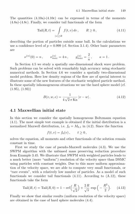
4.1 Maxwellian initial state 149
The quantities (4.10a)-(4.10c) can be expressed in terms of the moments(4.8a)-(4.8c). Finally, we consider tail functionals of the form
Tail(R, t) =∫
|v|≥R
f(t, v) dv , R ≥ 0 , (4.11)
describing the portion of particles outside some ball. In the calculations weuse a confidence level of p = 0.999 (cf. Section 3.1.4). Other basic parametersare
ν(n)(0) = n , ν(n)max = 4n , g(n)
max =2n
, κ = 1 .
In Section 4.5 we study a spatially one-dimensional shock wave problem.Such problems can be solved with remarkably high accuracy using stochasticnumerical methods. In Section 4.6 we consider a spatially two-dimensionalmodel problem. Here low density regions of the flow are of special interest toillustrate some of the new features of the stochastic weighted particle method.In these spatially inhomogeneous situations we use the hard sphere model (cf.(1.95), (1.93))
B(v, w, e) =1
4√
2 π Kn|v − w| . (4.12)
4.1 Maxwellian initial state
In this section we consider the spatially homogeneous Boltzmann equation(4.1). The most simple test example is obtained if the initial distribution is anormalized Maxwell distribution, i.e. f0 = M0,1 in (4.2). Since the function
f(t, v) = f0(v) , t ≥ 0 ,
solves the equation, all moments and other functionals of the solution remainconstant in time.
First we study the case of pseudo-Maxwell molecules (4.3). We use theSWPM algorithm with the unbiased mass preserving reduction procedurefrom Example 3.45. We illustrate that SWPM with weighted particles leads toa much better (more “uniform”) resolution of the velocity space than DSMCusing particles with constant weights. Due to this more uniform approxima-tion of the velocity space, we are able to compute very small functionals, or“rare events”, with a relatively low number of particles. As a model of suchfunctionals we consider tail functionals (4.11). According to (A.12), thesefunctionals take the form
Tail(R, t) = Tail(R, 0) = 1 − erf( R√
2
)+
2R√π
exp(− R2
2
). (4.13)
Finally we show that similar results (uniform resolution of the velocity space)are obtained in the case of hard sphere molecules (4.4).
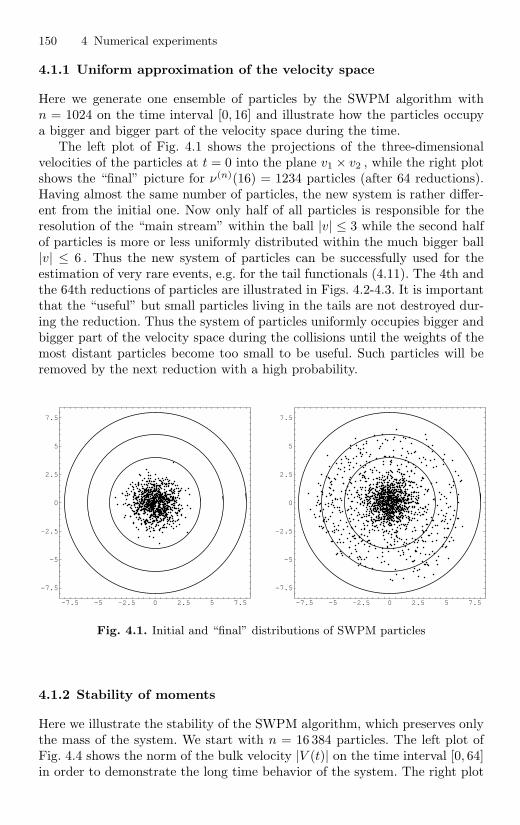
150 4 Numerical experiments
4.1.1 Uniform approximation of the velocity space
Here we generate one ensemble of particles by the SWPM algorithm withn = 1024 on the time interval [0, 16] and illustrate how the particles occupya bigger and bigger part of the velocity space during the time.
The left plot of Fig. 4.1 shows the projections of the three-dimensionalvelocities of the particles at t = 0 into the plane v1 × v2 , while the right plotshows the “final” picture for ν(n)(16) = 1234 particles (after 64 reductions).Having almost the same number of particles, the new system is rather differ-ent from the initial one. Now only half of all particles is responsible for theresolution of the “main stream” within the ball |v| ≤ 3 while the second halfof particles is more or less uniformly distributed within the much bigger ball|v| ≤ 6 . Thus the new system of particles can be successfully used for theestimation of very rare events, e.g. for the tail functionals (4.11). The 4th andthe 64th reductions of particles are illustrated in Figs. 4.2-4.3. It is importantthat the “useful” but small particles living in the tails are not destroyed dur-ing the reduction. Thus the system of particles uniformly occupies bigger andbigger part of the velocity space during the collisions until the weights of themost distant particles become too small to be useful. Such particles will beremoved by the next reduction with a high probability.
Fig. 4.1. Initial and “final” distributions of SWPM particles
4.1.2 Stability of moments
Here we illustrate the stability of the SWPM algorithm, which preserves onlythe mass of the system. We start with n = 16 384 particles. The left plot ofFig. 4.4 shows the norm of the bulk velocity |V (t)| on the time interval [0, 64]in order to demonstrate the long time behavior of the system. The right plot
-7.5 -5 -2.5 0 2.5 5 7.5
-7.5
-5
-2.5
0
2.5
5
7.5
-7.5 -5 -2.5 0 2.5 5 7.5
-7.5
-5
-2.5
0
2.5
5
7.5
4.1 Maxwellian initial state 151
Fig. 4.3. 64th reduction of particles, pseudo-Maxwell molecules
shows the temperature T (t) . These curves were obtained using N = 128independent ensembles.
There are errors in the bulk velocity and in the temperature due to non-conservative stochastic reduction of particles. But the deviation from the cor-rect constant value is small. However, it is always necessary to control thisdeviation.
4.1.3 Tail functionals
Here we provide the results of numerical computations of the tails (4.13) withdifferent values of the radius R ,
Tail(4, t) = 0.113398 . . . · 10−2 , (4.14a)
-7.5 -5 -2.5 0 2.5 5 7.5
-7.5
-5
-2.5
0
2.5
5
7.5
-7.5 -5 -2.5 0 2.5 5 7.5
-7.5
-5
-2.5
0
2.5
5
7.5
Fig. 4.2. 4th reduction of particles, pseudo-Maxwell molecules
-7.5 -5 -2.5 0 2.5 5 7.5
-7.5
-5
-2.5
0
2.5
5
7.5
-7.5 -5 -2.5 0 2.5 5 7.5
-7.5
-5
-2.5
0
2.5
5
7.5

152 4 Numerical experiments
0 10 20 30 40 50 60
0.0005
0.001
0.0015
0.002
0.0025
0.003
0 10 20 30 40 50 60
0.999
1
1.001
1.002
Fig. 4.4. Long time behavior of |V (t)| and T (t)
Tail(5, t) = 0.154404 . . . · 10−4 , (4.14b)Tail(6, t) = 0.748837 . . . · 10−7 , (4.14c)Tail(7, t) = 0.130445 . . . · 10−9 . (4.14d)
The number of particles in DSMC is n = 65 536 , while SWPM starts with n =16 384 particles. The computational time is then similar for both algorithms.Averages are taken over N = 4096 independent ensembles. Simulations areperformed on the time interval [0, 16] .
We observe that at the begin of the simulation the width of the confi-dence intervals is better for DSMC due to the higher number of particles. Thenumber of particles forming the tail remains almost constant for DSMC. Thecorresponding number increases for SWPM leading to smaller confidence in-tervals. In the figures confidence intervals obtained using DSMC are shown bythin solid lines, while confidence intervals obtained using SWPM are shownby thin dotted lines. The analytical values for the tails (4.14a)-(4.14d) aredisplayed by thick solid lines. In the figures showing the average numbers ofparticles forming the tails, the left plots corresponds to DSMC and the rightplots to SWPM.
In the case R = 4 , the tail formed using SWPM contains a rather largenumber of particles compared to DSMC (Fig. 4.6). The accuracy of bothmethods is similar (Fig. 4.5) because many of these particles are not responsi-ble for resolving this tail, their weights are too small. However, many of themplay an important role in resolving the smaller tails.
The resolution of the second tail (R = 5) becomes better for SWPM aftersome time. The width of the DSMC confidence intervals is almost two timeslarger (Fig. 4.7). Thus the results of SWPM can be reached using four timesmore independent ensembles and therefore four times more computationaltime. Thus we can say that SWPM is four times “faster” computing this tailwith similar accuracy. Fig. 4.8 shows the corresponding number of particlesin the second tail.
This tendency continues also for the tail with R = 6. Now the widthof the DSMC confidence intervals is four-five times larger (Fig. 4.9). ThusSWPM can be considered 16-25 times “faster” computing this tail with similar

4.1 Maxwellian initial state 153
accuracy. The number of particles in this tail for SWPM seems to be stillincreasing (Fig. 4.10). This means that the forming of this tail has not yetbeen finished.
Fig. 4.11 shows the results obtained using SWPM for the tail with R = 7 .There are no stable DSMC results for this very small tail. Even if the tail isstill not formed on this time interval and the number of particles for SWPMis still rapidly growing (Fig. 4.12) the analytical value of this functional isreached with considerable accuracy.
0 2.5 5 7.5 10 12.5 15
0.00112
0.001125
0.00113
0.001135
0.00114
0.001145
Fig. 4.5. Tail functional for R = 4
0 2.5 5 7.5 10 12.5 1574.2
74.25
74.3
74.35
74.4
74.45
0 2.5 5 7.5 10 12.5 150
2000
4000
6000
8000
10000
12000
14000
Fig. 4.6. Number of particles in the tail for R = 4
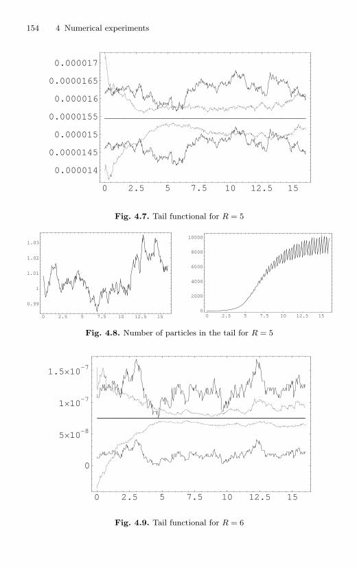
154 4 Numerical experiments
0 2.5 5 7.5 10 12.5 15
0.000014
0.0000145
0.000015
0.0000155
0.000016
0.0000165
0.000017
Fig. 4.7. Tail functional for R = 5
0 2.5 5 7.5 10 12.5 15
0.99
1
1.01
1.02
1.03
0 2.5 5 7.5 10 12.5 150
2000
4000
6000
8000
10000
Fig. 4.8. Number of particles in the tail for R = 5
0 2.5 5 7.5 10 12.5 15
0
5�10-8
1�10-7
1.5�10-7
Fig. 4.9. Tail functional for R = 6

4.1 Maxwellian initial state 155
0 2.5 5 7.5 10 12.5 15
0.004
0.0045
0.005
0.0055
0 2.5 5 7.5 10 12.5 150
1000
2000
3000
4000
Fig. 4.10. Number of particles in the tail for R = 6
0 2.5 5 7.5 10 12.5 15
-5�10-10
0
5�10-10
1�10-9
1.5�10-9
Fig. 4.11. Tail functional for R = 7
0 2.5 5 7.5 10 12.5 150
0.00001
0.00002
0.00003
0.00004
0.00005
0.00006
0 2.5 5 7.5 10 12.5 150
20
40
60
80
100
120
140
Fig. 4.12. Number of particles in the tail for R = 7
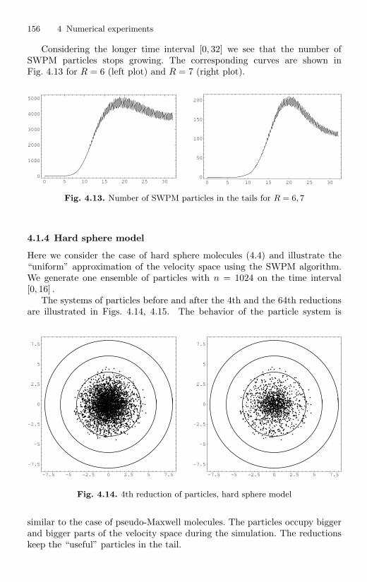
156 4 Numerical experiments
Considering the longer time interval [0, 32] we see that the number ofSWPM particles stops growing. The corresponding curves are shown inFig. 4.13 for R = 6 (left plot) and R = 7 (right plot).
0 5 10 15 20 25 300
1000
2000
3000
4000
5000
0 5 10 15 20 25 300
50
100
150
200
Fig. 4.13. Number of SWPM particles in the tails for R = 6, 7
4.1.4 Hard sphere model
Here we consider the case of hard sphere molecules (4.4) and illustrate the“uniform” approximation of the velocity space using the SWPM algorithm.We generate one ensemble of particles with n = 1024 on the time interval[0, 16] .
The systems of particles before and after the 4th and the 64th reductionsare illustrated in Figs. 4.14, 4.15. The behavior of the particle system is
Fig. 4.14. 4th reduction of particles, hard sphere model
similar to the case of pseudo-Maxwell molecules. The particles occupy biggerand bigger parts of the velocity space during the simulation. The reductionskeep the “useful” particles in the tail.
-7.5 -5 -2.5 0 2.5 5 7.5
-7.5
-5
-2.5
0
2.5
5
7.5
-7.5 -5 -2.5 0 2.5 5 7.5
-7.5
-5
-2.5
0
2.5
5
7.5

4.2 Relaxation of a mixture of two Maxwellians 157
Fig. 4.15. 64th reduction of particles, hard sphere model
4.2 Relaxation of a mixture of two Maxwellians
In this section we consider the spatially homogeneous Boltzmann equation(4.1) with the initial distribution
f0(v) = αMV1,T1(v) + (1 − α)MV2,T2(v) , 0 ≤ α ≤ 1 , (4.15)
which is a mixture of two Maxwell distributions. Fig. 4.16 shows a two-
-5-2.5
0
2.5
5-5
-2.5
0
2.5
5
0
0.02
0.04
0.06
0.08
-5-2.5
0
2.5
5-6 -4 -2 0 2 4 6
-6
-4
-2
0
2
4
6
Fig. 4.16. Initial distribution f0(v1, v2)
dimensional plot of the function
f0(v1, v2) =
∞∫−∞
f0(v1, v2, v3) dv3
-7.5 -5 -2.5 0 2.5 5 7.5
-7.5
-5
-2.5
0
2.5
5
7.5
-7.5 -5 -2.5 0 2.5 5 7.5
-7.5
-5
-2.5
0
2.5
5
7.5

158 4 Numerical experiments
as well as its contours for the set of parameters
V1 = (−2, 2, 0) , V2 = (2, 0, 0) , T1 = T2 = 1 , α = 1/2 . (4.16)
We first consider the case of pseudo-Maxwell molecules (4.3). Using theanalytic formulas from Section A.2, we study the convergence behavior ofDSMC and SWPM (with two different reduction procedures) with respect tothe number of particles. Then we study the approximation of tail functionals(4.11). According to (A.11), the initial and the asymptotic values of thesefunctionals are known, while analytical information about the time relaxationis not available. Finally we show that similar results (convergence with respectto the number of particles) are obtained in the case of hard sphere molecules(4.4).
Note that (cf. (A.7a)-(A.7c))
V = αV1 + (1 − α)V2 , (4.17a)
T = αT1 + (1 − α)T2 +13α(1 − α)|V1 − V2|2 , (4.17b)
M0 = α(T1 I + V1V
T1
)+ (1 − α)
(T2 I + V2V
T2
), (4.17c)
r0 = α(5T1 + |V1|2
)V1 + (1 − α)
(5T2 + |V2|2
)V2 , (4.17d)
s0 = α(|V1|4 + 15T 2
1 + 10T1 |V1|2)
+ (4.17e)
(1 − α)(|V2|4 + 15T 2
2 + 10T2 |V2|2),
where M0, r0, s0 are the initial values of the moments (4.8a)-(4.8c). Consider-ing the parameters (4.16), we obtain from (4.17a)-(4.17e)
V =
⎛⎝ 0
10
⎞⎠ , T =
83
, M0 =
⎛⎝ 5 −2 0
−2 3 00 0 1
⎞⎠ ,
r0 =
⎛⎝−4
130
⎞⎠ , s0 = 115 (4.18)
and from (A.18a)-(A.18c)
M(t) =13
⎛⎝ 8 0 0
0 11 00 0 8
⎞⎠+
13
⎛⎝ 7 −6 0
−6 −2 00 0 −5
⎞⎠ e−t/2 , (4.19a)
r(t) =13
⎛⎝ 0
430
⎞⎠− 1
3
⎛⎝12
40
⎞⎠ e−t/2 , (4.19b)
s(t) =4033
− 25 e−t/3 +253
e−t − 83
e−t/2 . (4.19c)

4.2 Relaxation of a mixture of two Maxwellians 159
Moreover, one obtains from (4.18) and (A.22)-(A.24)
τ(t) =13
⎛⎝ 7 −6 0
−6 −2 00 0 −5
⎞⎠ e−t/2 , q(t) = 0 , γ(t) = −25 e−t/3 +
253
e−t
so that the function (4.9) takes the form
Crit(t) =5
256
(30 e−2t − 180 e−4t/3 + 3072 e−t + 270 e−2t/3
)1/2
. (4.20)
4.2.1 Convergence of DSMC
Here we demonstrate the convergence of the DSMC method with respect to thenumber of particles n on some time interval [0, tmax] . For a given functionalΨ , the maximal error is defined as
Emax(Ψ) = max0≤k≤K
|Ψ(tk) − η(tk)| , (4.21)
where
tk = k∆ t , k = 0, . . . , K , ∆ t =tmax
K(4.22)
and K denotes the number of observation points. The “asymptotic” error isdefined as
E∞(Ψ) = |Ψ(tmax) − η(tmax)| . (4.23)
The quantity η in (4.21), (4.23) denotes the value of the functional calculatedby the algorithm and averaged over N independent runs (cf. (3.23)). We usethe parameters
N = 220 = 1048 576 , tmax = 16 . (4.24)
The thick solid lines in Fig. 4.17 correspond to the analytical solution(4.19a) for M11 . The pairs of thin solid lines represent the confidence inter-vals (3.25) for n = 16 and n = 64 (from above). The left plot shows theresults on the time interval [0, 1] illustrating that the initial condition is wellapproximated for both values of n . The right plot shows the results on thetime interval [4, 16] clearly indicating that the “asymptotic” error for n = 64 isfour times smaller than for n = 16 . Thus the convergence order of the system-atic error (3.24) O(n−1) can be seen. On the other hand, the thickness of theconfidence intervals representing the stochastic error (fluctuations) behavesas O(n−1/2) . This behavior is perfectly shown in Table 4.1. The numericalvalues of the errors (4.21) and (4.23) are displayed, respectively, in the secondand fourth columns. The sixth column shows the maximal thickness of theconfidence interval (CI). The third, fifth and seventh columns of this table

160 4 Numerical experiments
0 0.2 0.4 0.6 0.8
4.2
4.4
4.6
4.8
5
4 6 8 10 12 14 16
2.7
2.8
2.9
3
3.1
Fig. 4.17. Exact curve M11(t) and confidence intervals for n = 16, 64
Table 4.1. Numerical convergence of M11, DSMC
n Emax(M11) CF E∞(M11) CF CI(M11) CF
16 0.147 E-00 - 0.143 E-00 - 0.338E-02 -32 0.728 E-01 2.02 0.720 E-01 2.01 0.238E-02 1.4264 0.369 E-01 1.97 0.359 E-01 2.01 0.169E-02 1.41
128 0.189 E-01 1.95 0.183 E-01 1.96 0.119E-02 1.42256 0.959 E-02 1.97 0.920 E-02 1.99 0.853E-03 1.41
show the “convergence factors”, i.e. the quotients between the errors in twoconsecutive lines of the previous columns. Note that the asymptotic value ofthis moment (cf. (4.19a)) is (M∞)11 = 8/3. Thus the relative error for n = 256is only 0.35% .
Analogous results for the second component of the energy flux vector r2
are presented in Fig. 4.18 and Table 4.2. Note that the asymptotic value ofthis moment (cf. (4.19b)) is (r∞)2 = 43/3. Thus the relative error for n = 256is only 0.06% .
0 0.2 0.4 0.6 0.8
13
13.1
13.2
13.3
13.4
13.5
4 6 8 10 12 14 1614.05
14.1
14.15
14.2
14.25
14.3
Fig. 4.18. Exact curve r2(t) and confidence intervals for n = 16, 64
Results for the fourth moment s (4.17d) are presented in Fig. 4.19 andTable 4.3. Note that the asymptotic value of this moment (cf. (4.19c)) iss∞ = 403/3. Thus the relative error for n = 256 is only 0.8% .
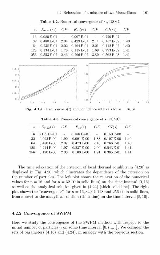
4.2 Relaxation of a mixture of two Maxwellians 161
Table 4.2. Numerical convergence of r2, DSMC
n Emax(r2) CF E∞(r2) CF CI(r2) CF
16 0.980 E-01 - 0.907 E-01 - 0.220 E-02 -32 0.480 E-01 2.04 0.429 E-01 2.11 0.157 E-02 1.4064 0.238 E-01 2.02 0.194 E-01 2.21 0.112 E-02 1.40
128 0.134 E-01 1.78 0.115 E-01 1.69 0.793 E-02 1.41256 0.553 E-02 2.43 0.296 E-02 3.89 0.562 E-03 1.41
0 0.2 0.4 0.6 0.8
115
115.5
116
116.5
117
117.5
4 6 8 10 12 14 16126
128
130
132
134
Fig. 4.19. Exact curve s(t) and confidence intervals for n = 16, 64
Table 4.3. Numerical convergence of s, DSMC
n Emax(s) CF E∞(s) CF CI(s) CF
16 0.189 E+01 - 0.186 E+01 - 0.150 E-00 -32 0.992 E-00 1.90 0.991E-00 1.88 0.107 E-00 1.4064 0.480 E-00 2.07 0.473E-00 2.10 0.766 E-01 1.40
128 0.244 E-00 1.97 0.237E-00 2.00 0.543 E-01 1.41256 0.120 E-00 2.03 0.108E-00 1.91 0.385 E-01 1.41
The time relaxation of the criterion of local thermal equilibrium (4.20) isdisplayed in Fig. 4.20, which illustrates the dependence of the criterion onthe number of particles. The left plot shows the relaxation of the numericalvalues for n = 16 and for n = 32 (thin solid lines) on the time interval [0, 16]as well as the analytical solution given in (4.22) (thick solid line). The rightplot shows the “convergence” for n = 16, 32, 64, 128 and 256 (thin solid lines,from above) to the analytical solution (thick line) on the time interval [8, 16] .
4.2.2 Convergence of SWPM
Here we study the convergence of the SWPM method with respect to theinitial number of particles n on some time interval [0, tmax] . We consider thesets of parameters (4.16) and (4.24), in analogy with the previous section.

162 4 Numerical experiments
0 2.5 5 7.5 10 12.5 150
0.2
0.4
0.6
0.8
1
8 10 12 14 160
0.02
0.04
0.06
0.08
Fig. 4.20. Criterion of local thermal equilibrium
Unbiased mass preserving reduction procedure
First we consider SWPM with the reduction measure from Example 3.45. Thetime behavior of the number of particles for n = 256 is illustrated in Fig. 4.21.The decreasing amplitude of particle number fluctuations is due to differenttime points the reductions took place for different independent ensembles.
0 2.5 5 7.5 10 12.5 15
300
400
500
600
700
800
Fig. 4.21. Number of SWPM particles for n = 256
The results, which are optically indistinguishable from those obtained us-ing DSMC, are presented in Tables 4.4-4.6.
Mass, momentum and energy preserving reduction procedure
Now we solve the same problem using SWPM with the reduction measure fromExample 3.46 (with k(i) = 3 and uniform σred). The results are presented inTables 4.7-4.9.
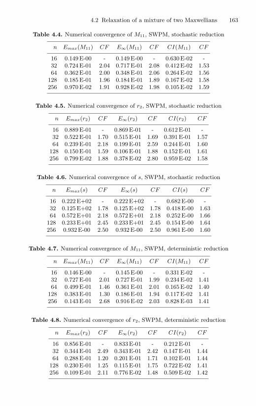
4.2 Relaxation of a mixture of two Maxwellians 163
Table 4.4. Numerical convergence of M11, SWPM, stochastic reduction
n Emax(M11) CF E∞(M11) CF CI(M11) CF
16 0.149 E-00 - 0.149 E-00 - 0.630E-02 -32 0.724 E-01 2.04 0.717 E-01 2.08 0.412E-02 1.5364 0.362 E-01 2.00 0.348 E-01 2.06 0.264E-02 1.56
128 0.185 E-01 1.96 0.184 E-01 1.89 0.167E-02 1.58256 0.970 E-02 1.91 0.928 E-02 1.98 0.105E-02 1.59
Table 4.5. Numerical convergence of r2, SWPM, stochastic reduction
n Emax(r2) CF E∞(r2) CF CI(r2) CF
16 0.889 E-01 - 0.869 E-01 - 0.612 E-01 -32 0.522 E-01 1.70 0.515 E-01 1.69 0.391 E-01 1.5764 0.239 E-01 2.18 0.199 E-01 2.59 0.244 E-01 1.60
128 0.150 E-01 1.59 0.106 E-01 1.88 0.152 E-01 1.61256 0.799 E-02 1.88 0.378 E-02 2.80 0.959 E-02 1.58
Table 4.6. Numerical convergence of s, SWPM, stochastic reduction
n Emax(s) CF E∞(s) CF CI(s) CF
16 0.222 E+02 - 0.222 E+02 - 0.682 E-00 -32 0.125 E+02 1.78 0.125 E+02 1.78 0.418 E-00 1.6364 0.572 E+01 2.18 0.572 E+01 2.18 0.252 E-00 1.66
128 0.233 E+01 2.45 0.233 E+01 2.45 0.154 E-00 1.64256 0.932 E-00 2.50 0.932E-00 2.50 0.961 E-00 1.60
Table 4.7. Numerical convergence of M11, SWPM, deterministic reduction
n Emax(M11) CF E∞(M11) CF CI(M11) CF
16 0.146 E-00 - 0.145 E-00 - 0.331E-02 -32 0.727 E-01 2.01 0.727 E-01 1.99 0.234E-02 1.4164 0.499 E-01 1.46 0.361 E-01 2.01 0.165E-02 1.40
128 0.383 E-01 1.30 0.186 E-01 1.94 0.117E-02 1.41256 0.143 E-01 2.68 0.916 E-02 2.03 0.828E-03 1.41
Table 4.8. Numerical convergence of r2, SWPM, deterministic reduction
n Emax(r2) CF E∞(r2) CF CI(r2) CF
16 0.856 E-01 - 0.833 E-01 - 0.212 E-01 -32 0.344 E-01 2.49 0.343 E-01 2.42 0.147 E-01 1.4464 0.288 E-01 1.20 0.201 E-01 1.71 0.102 E-01 1.44
128 0.230 E-01 1.25 0.115 E-01 1.75 0.722 E-02 1.41256 0.109 E-01 2.11 0.776 E-02 1.48 0.509 E-02 1.42

164 4 Numerical experiments
Table 4.9. Numerical convergence of s, SWPM, deterministic reduction
n Emax(s) CF E∞(s) CF CI(s) CF
64 0.156 E+02 - 0.156 E+02 - 0.645E-01 -128 0.127 E+02 1.22 0.127 E+02 1.22 0.463E-01 1.39256 0.861 E+01 1.48 0.861 E+01 1.48 0.335E-01 1.38
1048576 0.400 E-01 - 0.228 E-01 - - -
SWPM with deterministic reduction shows less stable convergence for theusual moments and unstable behavior for the moment s for small number ofparticles (n = 16, 32). However, increasing the number of particles (see lastrow of Table 4.9) leads to a convergent procedure even for this high moment.
4.2.3 Tail functionals
Here we study the time relaxation of tail functionals (4.11) and comparethe DSMC and SWPM algorithms. The parameters of the initial distribution(4.15) are
V1 = (96, 0, 0) , V2 = (−32/3, 0, 0) , T1 = T2 = 1 , α = 1/10
so that, according to (4.17a), (4.17b),
V = (0, 0, 0) , T = 1027/3 .
The asymptotic value of the tail functional takes the form (cf. (A.12))
Tail(R,∞) = 1 − erf( R√
2T
)+
2R√π T
exp(− R2
2T
).
In particular, one obtains
Tail(100,∞) = 0.202177 . . . · 10−5 ,
Tail(110,∞) = 0.102966 . . . · 10−6 ,
Tail(120,∞) = 0.388809 . . . · 10−8 ,
Tail(130,∞) = 0.108962 . . . · 10−9 .
The number of particles for DSMC is n = 65 536 . The initial number ofparticles for SWPM (with stochastic reduction) is n = 16 384 . The number ofindependent ensembles is N = 32 768 for DSMC and N = 16 384 for SWPM.For these choices the computational time for SWPM is approximately 2/3 ofthat for DSMC. Simulations are performed on the time interval [0, 32] .
The highly oscillating number of SWPM particles is shown in Fig. 4.22.The average number of particles is close to 40 000 . The time relaxation forTail(100, t) (obtained using both DSMC and SWPM) is shown in Fig. 4.23.
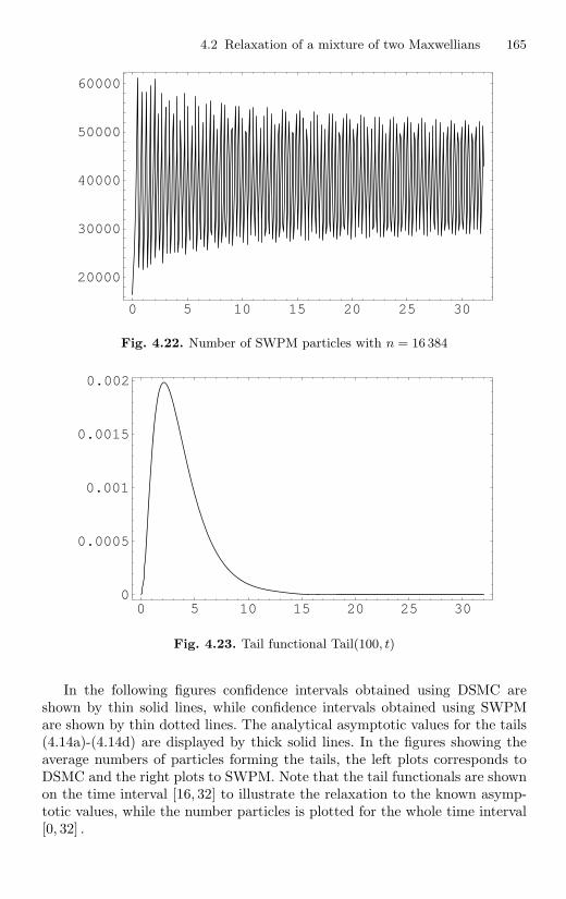
4.2 Relaxation of a mixture of two Maxwellians 165
0 5 10 15 20 25 30
20000
30000
40000
50000
60000
Fig. 4.22. Number of SWPM particles with n = 16 384
0 5 10 15 20 25 300
0.0005
0.001
0.0015
0.002
Fig. 4.23. Tail functional Tail(100, t)
In the following figures confidence intervals obtained using DSMC areshown by thin solid lines, while confidence intervals obtained using SWPMare shown by thin dotted lines. The analytical asymptotic values for the tails(4.14a)-(4.14d) are displayed by thick solid lines. In the figures showing theaverage numbers of particles forming the tails, the left plots corresponds toDSMC and the right plots to SWPM. Note that the tail functionals are shownon the time interval [16, 32] to illustrate the relaxation to the known asymp-totic values, while the number particles is plotted for the whole time interval[0, 32] .

166 4 Numerical experiments
We see in Fig. 4.24 that the width of the confidence intervals is similar forDSMC and for SWPM for the first tail functional with R = 100 . Fig. 4.25shows that both methods have only few particles forming the tail at the be-ginning of the simulation. Then SWPM produces much more particles in thetail and keeps them during the reductions while the corresponding numberfor DSMC just follows the functional to compute (cf. Fig. 4.23). Note thatthe tail formed using SWPM contains a rather large number of particles com-pared to DSMC. The accuracy is similar because many of these particles arenot responsible for resolving this tail, their weights are too small. Many ofthem play an important role resolving the tails for larger values of R .
As we see in Fig. 4.26 the resolution of the second tail (R = 110) isalready better for SWPM. The results of SWPM can be reached by DSMCusing three-four times more computational time. Thus we can say that SWPMis three-four times “faster” computing this tail with similar accuracy. Fig. 4.27shows the corresponding numbers of particles in the second tail.
This tendency continues also for the tail with R = 120 as shown inFig. 4.28. Now the width of the DSMC confidence intervals is about threetimes larger. Thus SWPM can be considered about ten times faster comput-ing this tail with similar accuracy. The number of SWPM particles in this tailshown in Fig. 4.29 is now decreasing in time. However it is still rather big.
Figs. 4.30 and 4.31 show the results obtained using SWPM for the tailwith R = 130 . There are no stable DSMC results for this very small tail,while SWPM still reproduces the asymptotic analytical value.
17.5 20 22.5 25 27.5 302�10-6
3�10-6
4�10-6
5�10-6
6�10-6
7�10-6
8�10-6
Fig. 4.24. Tail functional for R = 100
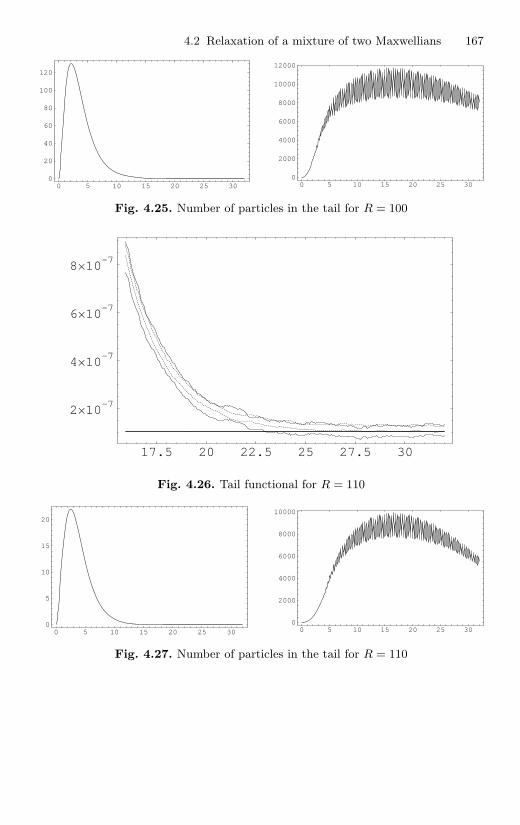
4.2 Relaxation of a mixture of two Maxwellians 167
0 5 10 15 20 25 300
20
40
60
80
100
120
0 5 10 15 20 25 300
2000
4000
6000
8000
10000
12000
Fig. 4.25. Number of particles in the tail for R = 100
17.5 20 22.5 25 27.5 30
2�10-7
4�10-7
6�10-7
8�10-7
Fig. 4.26. Tail functional for R = 110
0 5 10 15 20 25 300
5
10
15
20
0 5 10 15 20 25 300
2000
4000
6000
8000
10000
Fig. 4.27. Number of particles in the tail for R = 110

168 4 Numerical experiments
17.5 20 22.5 25 27.5 300
2�10-8
4�10-8
6�10-8
8�10-8
Fig. 4.28. Tail functional for R = 120
0 5 10 15 20 25 300
0.5
1
1.5
2
0 5 10 15 20 25 300
2000
4000
6000
Fig. 4.29. Number of particles in the tail for R = 120
17.5 20 22.5 25 27.5 300
1�10-9
2�10-9
3�10-9
4�10-9
5�10-9
6�10-9
7�10-9
Fig. 4.30. Tail functional for R = 130

4.2 Relaxation of a mixture of two Maxwellians 169
0 5 10 15 20 25 300
0.05
0.1
0.15
0.2
0 5 10 15 20 25 300
1000
2000
3000
4000
5000
Fig. 4.31. Number of particles in the tail for R = 130
4.2.4 Hard sphere model
Here we consider the case of hard sphere molecules (4.4) and study conver-gence of DSMC and SWPM with respect to the number of particles. Sinceexact time relaxation curves are not available, we illustrate the “convergence”plotting the DSMC curves for n = 16, 64, 256 and N = 65 536 independentensembles. The SWPM results are optically indistinguishable from those ob-tained by DSMC. Simulations are performed on the time interval [0, 4] .
Results are given for the second moments M11(t),M12(t),M22(t),M33(t)in Figs. 4.32, 4.33, for the third moments r1(t), r2(t) in Fig. 4.34 and for thefourth moment s(t) in Fig. 4.35. Note that the asymptotic values of all thesemoments are identical to those given in (4.18), (4.19a)-(4.19c) for pseudo-Maxwell molecules.
0 1 2 3 4
3
3.5
4
4.5
5
0 1 2 3 4-2
-1.5
-1
-0.5
0
Fig. 4.32. Time relaxation of the moments M11(t), M12(t) for n = 16, 64, 256
Fig. 4.36 shows the whole number of collisions as well as the number offictitious collisions for both DSMC (left plot) and SWPM (right plot) meth-ods. Note that fictitious collisions will necessarily appear for DSMC too, if themodel of interaction is different from pseudo-Maxwell molecules. The numberof particles for DSMC is n = 256 . The initial number of particles for SWPM(with stochastic reduction) is n = 64 . Note that the number of SWPM col-lisions is significantly bigger than the number of DSMC collisions due to thecomplicated collision procedure involving more fictitious collisions.
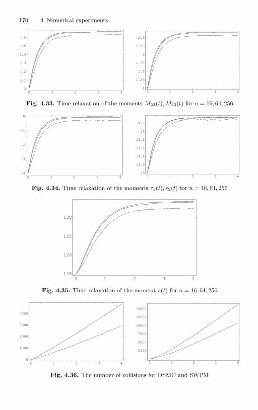
170 4 Numerical experiments
0 1 2 3 43
3.1
3.2
3.3
3.4
3.5
3.6
0 1 2 3 41
1.25
1.5
1.75
2
2.25
2.5
Fig. 4.33. Time relaxation of the moments M22(t), M33(t) for n = 16, 64, 256
0 1 2 3 4-4
-3
-2
-1
0
0 1 2 3 413
13.2
13.4
13.6
13.8
14
14.2
Fig. 4.34. Time relaxation of the moments r1(t), r2(t) for n = 16, 64, 256
0 1 2 3 4115
120
125
130
Fig. 4.35. Time relaxation of the moment s(t) for n = 16, 64, 256
0 1 2 3 40
1000
2000
3000
4000
0 1 2 3 40
2500
5000
7500
10000
12500
15000
Fig. 4.36. The number of collisions for DSMC and SWPM

4.3 BKW solution of the Boltzmann equation 171
4.3 BKW solution of the Boltzmann equation
In this section we consider the BKW solution (A.35) of the spatially homo-geneous Boltzmann equation (4.1) with the collision kernel (4.3). Taking intoaccount that (cf. (A.32))
α =14
π∫0
sin3 θ dθ =13
and choosing the set of parameters (cf. (A.36))
β0 = 2/3 , = 1 , T = 1 ,
one obtains
f(t, v) =1
(2π)3/2
(β(t) + 1
)3/2(
1 + β(t)(β(t) + 1
2|v|2 − 3
2
))e−
β(t)+12 |v|2 ,
where (cf. (A.34))
β(t) =2 e−t/6
5 − 2 e−t/6.
Fig. 4.37 shows a two-dimensional plot of the function
f0(v1, v2) =
∞∫−∞
f0(v1, v2, v3) dv3 =5
18π
(1 +
56(v2
1 + v22))e−
56 (v2
1 + v22)
and its contours.We study the time relaxation of the functionals (cf. (A.37))
∫R3
|v| f(t, v) dv =(
2π
)1/2β(t) + 2
(β(t) + 1)1/2, (4.26a)
∫R3
|v|3 f(t, v) dv = 4(
2π
)1/2 3β(t) + 2(β(t) + 1)3/2
, (4.26b)
∫R3
|v|10 f(t, v) dv = 10 3955β(t) + 1
(β(t) + 1)5. (4.26c)
According to (A.38), the function (4.9) representing the criterion of localequilibrium takes the form
Crit(t) =√
3025
e−t/3 . (4.27)
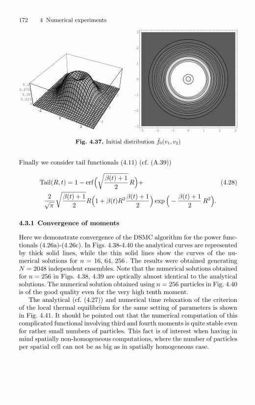
172 4 Numerical experiments
-2
0
2
-2
0
2
00.0250.05
0.075
0.1
-2
0
2-3 -2 -1 0 1 2 3
-3
-2
-1
0
1
2
3
Fig. 4.37. Initial distribution f0(v1, v2)
Finally we consider tail functionals (4.11) (cf. (A.39))
Tail(R, t) = 1 − erf(√β(t) + 1
2R)+ (4.28)
2√π
√β(t) + 1
2R(1 + β(t)R2 β(t) + 1
2
)exp(− β(t) + 1
2R2).
4.3.1 Convergence of moments
Here we demonstrate convergence of the DSMC algorithm for the power func-tionals (4.26a)-(4.26c). In Figs. 4.38-4.40 the analytical curves are representedby thick solid lines, while the thin solid lines show the curves of the nu-merical solutions for n = 16, 64, 256 . The results were obtained generatingN = 2048 independent ensembles. Note that the numerical solutions obtainedfor n = 256 in Figs. 4.38, 4.39 are optically almost identical to the analyticalsolutions. The numerical solution obtained using n = 256 particles in Fig. 4.40is of the good quality even for the very high tenth moment.
The analytical (cf. (4.27)) and numerical time relaxation of the criterionof the local thermal equilibrium for the same setting of parameters is shownin Fig. 4.41. It should be pointed out that the numerical computation of thiscomplicated functional involving third and fourth moments is quite stable evenfor rather small numbers of particles. This fact is of interest when having inmind spatially non-homogeneous computations, where the number of particlesper spatial cell can not be as big as in spatially homogeneous case.

4.3 BKW solution of the Boltzmann equation 173
0 5 10 15 20 25 30
1.6
1.61
1.62
1.63
1.64
Fig. 4.38. Power functional (4.26a)
0 5 10 15 20 25 30
6
6.1
6.2
6.3
Fig. 4.39. Power functional (4.26b)

174 4 Numerical experiments
0 5 10 15 20 25 30
4000
5000
6000
7000
8000
9000
10000
Fig. 4.40. Power functional (4.26c)
0 5 10 15 20 25 300
0.05
0.1
0.15
0.2
Fig. 4.41. Criterion of the local thermal equilibrium (4.27)
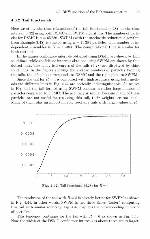
4.3 BKW solution of the Boltzmann equation 175
4.3.2 Tail functionals
Here we study the time relaxation of the tail functional (4.28) on the timeinterval [0, 32] using both DSMC and SWPM algorithms. The number of parti-cles for DSMC is n = 65 536 . SWPM (with the stochastic reduction algorithmfrom Example 3.45) is started using n = 16 384 particles. The number of in-dependent ensembles is N = 16 384 . The computational time is similar forboth methods.
In the figures confidence intervals obtained using DSMC are shown by thinsolid lines, while confidence intervals obtained using SWPM are shown by thindotted lines. The analytical curves of the tails (4.28) are displayed by thicksolid lines. In the figures showing the average numbers of particles formingthe tails, the left plots corresponds to DSMC and the right plots to SWPM.
Since the tail for R = 4 is computed with high accuracy using both meth-ods the different lines in Fig. 4.42 are optically indistinguishable. As we seein Fig. 4.43 the tail formed using SWPM contains a rather large number ofparticles compared to DSMC. The accuracy is similar because many of theseparticles are not useful for resolving this tail, their weights are too small.Many of them play an important role resolving tails with larger values of R .
0 5 10 15 20 25 30
0.0002
0.0004
0.0006
0.0008
0.001
Fig. 4.42. Tail functional (4.28) for R = 4
The resolution of the tail with R = 5 is already better for SWPM as shownin Fig. 4.44. In other words, SWPM is two-three times “faster” computingthis tail with similar accuracy. Fig. 4.45 displays the corresponding numbersof particles.
This tendency continues for the tail with R = 6 as shown in Fig. 4.46.Now the width of the DSMC confidence intervals is about three times larger.
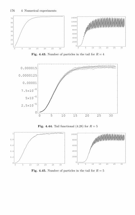
176 4 Numerical experiments
0 5 10 15 20 25 30
10
20
30
40
50
60
70
0 5 10 15 20 25 300
2000
4000
6000
8000
10000
12000
14000
Fig. 4.43. Number of particles in the tail for R = 4
0 5 10 15 20 25 300
2.5�10-6
5�10-6
7.5�10-6
0.00001
0.0000125
0.000015
Fig. 4.44. Tail functional (4.28) for R = 5
0 5 10 15 20 25 300
0.2
0.4
0.6
0.8
1
0 5 10 15 20 25 300
2000
4000
6000
8000
10000
Fig. 4.45. Number of particles in the tail for R = 5

4.3 BKW solution of the Boltzmann equation 177
Thus SWPM can be considered about nine times “faster” computing this tailwith similar accuracy. The number of particles in this tail for DSMC is nowvery small as shown in Fig. 4.47, while the number of SWPM particles is quitestable apart from the regular fluctuations due to reductions.
0 5 10 15 20 25 300
2�10-8
4�10-8
6�10-8
8�10-8
1�10-7
1.2�10-7
Fig. 4.46. Tail functional (4.28) for R = 6
0 5 10 15 20 25 300
0.001
0.002
0.003
0.004
0.005
0.006
0 5 10 15 20 25 300
1000
2000
3000
4000
Fig. 4.47. Number of particles in the tail for R = 6
Figs. 4.48 and 4.49 show the results obtained using SWPM for the tailwith R = 7 . There are no stable DSMC results for this very small tail, whileSWPM reproduces the analytical curve on the whole time interval.
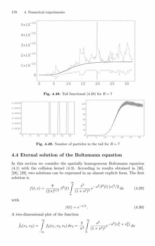
178 4 Numerical experiments
0 5 10 15 20 25 30
0
1�10-10
2�10-10
3�10-10
4�10-10
5�10-10
Fig. 4.48. Tail functional (4.28) for R = 7
0 5 10 15 20 25 300
0.00001
0.00002
0.00003
0.00004
0.00005
0.00006
0 5 10 15 20 25 300
20
40
60
80
100
120
Fig. 4.49. Number of particles in the tail for R = 7
4.4 Eternal solution of the Boltzmann equation
In this section we consider the spatially homogeneous Boltzmann equation(4.1) with the collision kernel (4.3). According to results obtained in [30],[28], [29], two solutions can be expressed in an almost explicit form. The firstsolution is
f(t, v) =8
(2π)5/2β3(t)
∞∫0
s3
(1 + s2)2e−s2β2(t) |v|2/2 ds (4.29)
with
β(t) = e−t/3 . (4.30)
A two-dimensional plot of the function
f0(v1, v2) =
∞∫−∞
f0(v1, v2, v3) dv3 =2π2
∞∫0
s2
(1 + s2)2e−s2(v2
1 + v22) ds
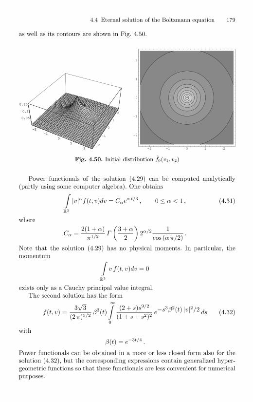
4.4 Eternal solution of the Boltzmann equation 179
as well as its contours are shown in Fig. 4.50.
-2-1
0
1
2-2
-1
0
1
2
0.05
0.1
0.15
-2-1
0
1
2 -2 -1 0 1 2
-2
-1
0
1
2
Fig. 4.50. Initial distribution f0(v1, v2)
Power functionals of the solution (4.29) can be computed analytically(partly using some computer algebra). One obtains∫
R3
|v|αf(t, v)dv = Cαeα t/3 , 0 ≤ α < 1 , (4.31)
where
Cα =2(1 + α)
π1/2Γ
(3 + α
2
)2α/2 1
cos (α π/2).
Note that the solution (4.29) has no physical moments. In particular, themomentum ∫
R3
v f(t, v)dv = 0
exists only as a Cauchy principal value integral.The second solution has the form
f(t, v) =3√
3(2π)5/2
β3(t)
∞∫0
(2 + s)s9/2
(1 + s + s2)2e−s3β2(t) |v|2/2 ds (4.32)
with
β(t) = e−3t/4 .
Power functionals can be obtained in a more or less closed form also for thesolution (4.32), but the corresponding expressions contain generalized hyper-geometric functions so that these functionals are less convenient for numericalpurposes.

180 4 Numerical experiments
4.4.1 Power functionals
The function ∫R3
|v|1/2f(t, v) dv =6
21/4 π1/2Γ(7
4
)et/6 (4.33)
is used for numerical tests. The most interesting thing with this function isthat it is unbounded in time. Since every DSMC simulation conserves energy(which increases with increasing number of particles and independent ensem-bles), the numerical curves for the power functional (4.31) can not follow theanalytic solution (4.33) to infinity. Thus they will converge to some constantvalue depending on the number of particles and on the number of independentensembles. We illustrate this behavior in Fig. 4.51, where the analytic curve(4.33) is presented with the thick solid line, while three thin solid lines showthe numerical approximations obtained for n = 4096, 16 384 and 262 144 par-ticles and N = 8 independent ensembles on the time interval [0, 64] . It canbe clearly seen that for larger values of n the curves follow the exact solutionfor longer time and converge to a larger value.
0 10 20 30 40 50 60
10
20
30
40
50
60
Fig. 4.51. Power functional (4.33)
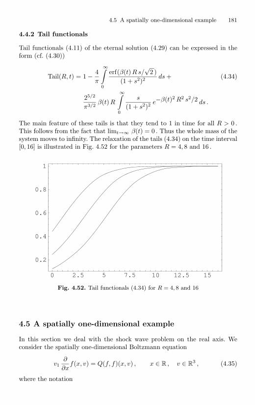
4.5 A spatially one-dimensional example 181
4.4.2 Tail functionals
Tail functionals (4.11) of the eternal solution (4.29) can be expressed in theform (cf. (4.30))
Tail(R, t) = 1 − 4π
∞∫0
erf(β(t)R s/√
2 )(1 + s2)2
ds + (4.34)
25/2
π3/2β(t)R
∞∫0
s
(1 + s2)2e−β(t)2 R2 s2/2 ds .
The main feature of these tails is that they tend to 1 in time for all R > 0 .This follows from the fact that limt→∞ β(t) = 0 . Thus the whole mass of thesystem moves to infinity. The relaxation of the tails (4.34) on the time interval[0, 16] is illustrated in Fig. 4.52 for the parameters R = 4, 8 and 16 .
0 2.5 5 7.5 10 12.5 15
0.2
0.4
0.6
0.8
1
Fig. 4.52. Tail functionals (4.34) for R = 4, 8 and 16
4.5 A spatially one-dimensional example
In this section we deal with the shock wave problem on the real axis. Weconsider the spatially one-dimensional Boltzmann equation
v1∂
∂xf(x, v) = Q(f, f)(x, v) , x ∈ R , v ∈ R
3 , (4.35)
where the notation

182 4 Numerical experiments
(4.36)
Q(f, f)(x, v) =∫R3
∫S2
B(v, w, e)(f(x, v′)f(x,w′) − f(x, v)f(x,w)
)de dw
is used and the post-collision velocities are defined in (1.6). Since the domain inthe physical space is unbounded one has to impose some additional conditionsat infinity on the distribution function. We assume
limx→−∞ f(x, v) = fM−(v) , lim
x→∞ f(x, v) = fM+(v) , (4.37)
where
fM±(v) =±
(2π T±)3/2exp(−|v − u±e1|2
2T±
), v ∈ R
3 . (4.38)
The parameters ±, T± and u± are positive numbers, while e1 = (1, 0, 0)T isthe first canonical unit vector.
4.5.1 Properties of the shock wave problem
Here we collect some properties of the steady state problem (4.35). The mo-ment equations (1.67) take the form
d
dx
( u)
= 0 , (4.39a)
d
dx
(p11 + u2
)= 0 , (4.39b)
d
dx
(q1 + p11 u +
(e +
12u2
)u)
= 0 , (4.39c)
where is the density, u is the first component of the bulk velocity, p11 isthe first component of the stress tensor, e is the internal energy and q1 is thefirst component of the heat flux vector. Thus the quantities in parentheses in(4.39a)-(4.39c) are some constants
(x)u(x) = c1 , (4.40a)p11(x) + (x)u2(x) = c2 , (4.40b)
q1(x) + p11(x)u(x) + (x)(e(x) +
12u2(x)
)u(x) = c3 . (4.40c)
If x → ±∞ then the gas tends to the equilibrium state corresponding to theconditions (4.37) so that
limx→±∞ (x) = ± ,
limx→±∞u(x) = u± ,

4.5 A spatially one-dimensional example 183
limx→±∞ p11(x) = ±T± ,
limx→±∞ q1(x) = 0 ,
limx→±∞ e(x) =
32T± .
Here the relations p(x) = (x)T (x) and T (x) = 2/3 e(x) have been used. Theparameters of the Maxwell distributions (4.38) are therefore related to eachother as
c1 = − u− = + u+ , (4.41a)
c2 = −(T− + u2
−)
= +
(T+ + u2
+
), (4.41b)
c3 = −u−(5
2T− +
12u2−)
= +u+
(52
T+ +12u2
+
). (4.41c)
These are the Rankine-Hugoniot conditions for shock waves in an idealcompressible fluid.
Introducing the Mach number (cf. (1.49))
M(x) =u(x)√53 T (x)
, M± =u±√53 T±
we can rewrite the quantities u−, +, u+, T+ and M+ in terms of the quantities−,M− and T− as
u− = M−
√53
T− , (4.42a)
+ =4M2
−3 + M2
−− , (4.42b)
u+ =3 + M2
−4M2
−u− , (4.42c)
T+ =5M4
− + 14M2− − 3
16M2−
T− , (4.42d)
M+ =3 + M2
−√5M4− + 14M2− − 3
. (4.42e)
The formulas (4.42a)–(4.42e) allow us the construction of different shock wavesfor numerical purposes.
One of the interesting features of the shock wave problem is the temper-ature overshoot downstream. To explain this phenomenon we consider thelongitudinal temperature defined as
T‖(x) =p11(x)(x)
,
184 4 Numerical experiments
where the component p11 of the stress tensor P is given by
p11(x) =∫R3
(v1 − u(x))2f(x, v) dv .
Using the relations (4.40b), (4.40a) we rewrite the longitudinal temperaturein the form
T‖(x) =c2
(x)− u2(x) =
c2
(x)− c2
1
2(x).
The constants c1 and c2 are related to the upstream values −, T− and M−as (cf. (4.42a))
c1 = − M−
√53
T− , c2 = − T− + − M2−
53
T− .
Thus we get
T‖(x) =T−3
((3 + 5M2
−)( −
(x)
)− 5M2
−( −
(x)
)2).
The function T‖ can be considered as a quadratic function of the variablez = −/ and achieves its maximum
T ∗‖ =
(3 + 5M2
−)2
60M2−T− (4.43)
at
z∗ =−∗
=3 + 5M2
−10M2−
.
This maximum will be reached only if the condition − < ∗ < + or equiva-lently (cf. (4.42b))
1 <10M2
−3 + 5M2−
<4M2
−3 + M2−
is fulfilled. Thus the condition for the temperature overshoot of the longitu-dinal temperature is
M− >
√95
. (4.44)
The overshoot itself can be expressed using (4.42d) and (4.43) as
T ∗‖
T+=
4(3 + 5M2
−)2
75M4− + 210M2− − 45> 1 for M− >
√95
.

4.5 A spatially one-dimensional example 185
Note that the maximal value of the longitudinal temperature given in (4.43)is known analytically while the position x∗ of this maximum with respect tothe space coordinate x
x∗ : (x∗) = ∗ = −10M2
−3 + 5M2−
(4.45)
can be determined only numerically.
4.5.2 Mott-Smith model
Here we describe the Mott-Smith ansatz for the distribution function f as anx−dependent convex combination of the two given Maxwellians,
fMS(x, v) = a(x) fM−(v) + (1 − a(x)) fM+(v) , (4.46)0 ≤ a(x) ≤ 1 , x ∈ R .
The function fMS can not satisfy the Boltzmann equation (4.35). Thus theresiduum
RMS(x, v) = v1∂
∂xfMS(x, v) − Q(fMS , fMS)(x, v)
is not identical to zero. The main idea of the Mott-Smith approach was tomultiply the residuum RMS by a test function ϕ, integrate the result over thewhole velocity space R
3 and then set the result of the integration to zero, i.e.∫R3
RMS(x, v)ϕ(v) dv = 0 . (4.47)
Thus the Mott-Smith ansatz is a very simple example of what we call nowGalerkin-Petrov solution of an operator equation. Using the special form of thefunction fMS defined in (4.46) we can easily derive from (4.47) the ordinarydifferential equation for the function a
d a
d x= β a(1 − a) , x ∈ R . (4.48)
The constant β in (4.48) is defined as
β = 2
∫R3
Q(fM− , fM+)ϕ(v) dv
∫R3
v1
(fM−(v) − fM+(v)
)ϕ(v) dv
(4.49)
provided that the denominator does not vanish. Equation (4.48) can be solvedimmediately giving

186 4 Numerical experiments
a(x) =eβ(x−x0)
1 + eβ(x−x0), x ∈ R .
This solution automatically fulfils the conditions for the function a at ±∞ forall negative values of the constant β
limx→−∞ a(x) = 1 , lim
x→+∞ a(x) = 0 .
Thus the integration constant x0 which defines the “center” of the Mott-Smithshock
fMS(x0, v) =12
fM−(v) +12
fM+(v)
can not be determined from the conditions at infinity. The calculation ofthe constant β , which is responsible for the “thickness” of the Mott-Smithshock, in a closed form is technically impossible even for very simple testfunctions ϕ (except the case of pseudo-Maxwell molecules). Thus it is moreconvenient to consider the Mott-Smith ansatz as the following two-parametric(β < 0 , x0 ∈ R) family
fMS(x, v) =eβ(x−x0)
1 + eβ(x−x0)fM−(v) +
11 + eβ(x−x0)
fM+(v) . (4.50)
Note that this distribution function does not really depend on three compo-nents of the velocity v. If we switch to the polar coordinates (r, ϕ) in the planev2 × v3 we obtain
fMS(x, v1, r) = a(x)−
(2π T−)3/2exp(− (v1 − u−)2 + r2
2T−
)+
(1 − a(x))+
(2π T+)3/2exp(− (v1 − u+)2 + r2
2T+
).
We discuss now some properties of the distribution function fMS . Fromthe analytic expression (4.50) we compute the main physical quantities of thisdistribution. The density is
MS(x) =∫R3
fMS(x, v) dv = a(x) − + (1 − a(x)) + . (4.51)
Computing the first component of the momentum
MS(x)uMS(x) =∫R3
v1 fMS(x, v) dv = a(x) −u− + (1 − a(x)) +u+ = c1
we can see that this is constant, i.e. equation (4.40a) is fulfilled. For the firstcomponent of the stress tensor we obtain with (4.41b) the expression

4.5 A spatially one-dimensional example 187
(p11
)MS
(x) =∫R3
(v1 − uMS(x))2 fMS(x, v) dv = a(x)−(T− + u2
−)
+
(1 − a(x))+
(T+ + u2
+
)− MS(x)u2
MS(x) = c2 − MS(x)u2MS(x) .
Thus equation (4.40b) is also fulfilled. Now we are able to compute an expres-sion for the Mott-Smith temperature
TMS(x) =1
3 MS(x)
(∫R3
∣∣∣v − uMS(x)(1, 0, 0)T∣∣∣2 fMS(x, v) dv
)
=1
3 MS(x)
((p11
)MS
(x) − 2 a(x)−T− + 2 (1 − a(x))+T+
).
Computing the first component of the heat flux vector and using the property(4.41c) we can see that also equation (4.40c) is fulfilled,
(q1
)MS
(x) =12
∫R3
∣∣∣v − uMS(x)(1, 0, 0)T∣∣∣2 (v1 − uMS(x)) fMS(x, v) dv =
a(x)−u−(5
2T− +
12u2−)
+ (1 − a(x))+u+
(52T+ +
12u2
+
)−
(p11
)MS
(x)uMS(x) − MS(x)uMS(x)(3
2TMS(x) +
12u2
MS(x))
= c3 −(p11
)MS
(x)uMS(x) − MS(x)uMS(x)(3
2TMS(x) +
12u2
MS(x))
.
Thus the physical quantities of the Mott-Smith distribution fulfil the samesystem of algebraic equations as the solution of the Boltzmann equation.However the system (4.40a)–(4.40c) of three equations contains five unknownfunctions , u, p11, T and q1. As we will see later the physical quantities of theMott-Smith distribution will differ from those obtained solving the Boltzmannequation (4.35) numerically.
Since the physical quantities of the Mott-Smith distribution function fulfilthe same equations, we deduce the same property for the longitudinal temper-ature T‖,MS . Its maximal value is identical to those of the Boltzmann equation(cf. (4.43)
T ∗‖,MS =
(3 + 5M2
−)2
60M2−T− .
However the position of this maximal value can now be computed analyticallyas
x∗ = x0 + β ln( 2M2
−(5M2− − 9)
(M2− + 3)(5M2− − 3)
),

188 4 Numerical experiments
using the formulas for the density (4.51) and for the position of the maximum(4.45). Note that the maximum of the longitudinal temperature occurs onlyif M2
− > 9/5 (cf. (4.44)).The formula for the density (4.51) allows us the exact computation of the
thickness of the shock using the definition
Ls,MS =+ − −
max ′MS(x). (4.52)
We obtain that the density reaches its maximal slope at x = x0 and thecorresponding thickness of the shock is
Ls,MS = 4+ − −
β.
Thus the parameter β is directly responsible for the thickness of the shock inthe Mott-Smith model. Later we will determine both parameters x0 and β us-ing numerical results for the value Ls obtained from the stochastic simulationof the Boltzmann equation.
Another interesting property of the Mott-Smith distribution function(4.50) is the following. Let
S3 ={
v ∈ R3 : fM−(v) = fM+(v)
}⊂ R
3
denote the set of such velocities for which both upstream and downstreamMaxwell distributions are equal. This set is a sphere
(v1 − u∗)2 + v22 + v2
3 = R2
with
u∗ =T+u− − T−u+
T+ − T−and
R2 =T+T−
T+ − T−
(ln(
−+
)2(T+
T−
)3
+(u+ − u−)2
T+ − T−
).
The distribution function (4.50) is constant with respect to the variable x onthe sphere S3 , i.e.
fMS(x, v) = a(x)fM−(v) + (1 − a(x))fM+(v) = fM−(v) = fM+(v) , v ∈ S3 .
The one-dimensional distribution functions for the Mott-Smith model
f(1)MS(x, v1) =
∞∫−∞
∞∫−∞
fMS(x, v) dv2 dv3
= a(x)−
(2π T−)1/2exp(− (v1 − u−)2
2T−
)+ (4.53)
(1 − a(x))+
(2π T+)1/2exp(− (v1 − u+)2
2T+
)

4.5 A spatially one-dimensional example 189
have two common points (for different x) at
v±1 = u∗ ± R . (4.54)
4.5.3 DSMC calculations
Since stochastic numerical algorithms for the Boltzmann equation are genuinetime-dependent methods, we start this subsection rewriting the steady stateproblem (4.35) on the whole real axis as a time-dependent problem on a finiteinterval,
∂
∂tf + v1
∂
∂xf = Q(f, f) , t > 0 , 0 < x < L , v ∈ R
3 ,
where L > 0 is the first “discretization parameter”. The conditions at infinity(4.37) are now transformed into inflow boundary conditions (cf. (1.36)) on theends of the interval [0, L] ,
f(t, 0, v) = fM−(v) , f(t, L, v) = fM+(v) .
We now need also an initial condition for t = 0 . This can be chosen in anartificial way, in order to reach the steady state solution fast. The choice
f(0, x, v) ={
fM−(v) , 0 ≤ x ≤ L/2 ,fM+(v) , L/2 < x ≤ L ,
is very convenient for numerical tests. For the parameters
− = 1 , T− = 3 , M− = 3 , (4.55)
one obtains according to (4.42a)–(4.42e)
u− = 3√
5 , + = 3 , T+ = 11 , M+ =√
33 /11 , u+ =√
5 . (4.56)
We use the value L = 2 for the interval length and the Knudsen numberKn = 0.05 . The discretization parameters of the problem are
nx = 1024 , ∆x = L/nx = 0.1953125 · 10−2 ,
∆t = 0.291155 · 10−3 . (4.57)
The time discretization parameter ∆t is chosen on such a way that a particlein in the undisturbed gas upstream having the typical velocity v = u− willcross exactly one spatial cell during the time interval ∆t. We initially use 8 192particles per spatial cell to resolve the density − = 1 in the undisturbed gasupstream. Thus the total number of particles in the computational domainwas about 1.6 · 107. After formation of the shock 4 096 time averaging stepswere realised in order to reduce the stochastic fluctuations.
In Fig. 4.53 the density and the first component u of the bulk velocityare presented. In Fig. 4.54 we show the profiles of the first component p11 ofthe stress tensor as well as of the pressure p = T . In Fig. 4.55 the profilesof the temperature T and of the Mach number are drawn. Finally, Fig. 4.56shows the first component q1 of the heat flux vector and the criterion of localthermal equilibrium Crit computed corresponding to (1.91).

190 4 Numerical experiments
0 0.5 1 1.5 21
1.5
2
2.5
3
0 0.5 1 1.5 2
5
10
15
20
25
30
Fig. 4.53. � and u
0 0.5 1 1.5 2
5
10
15
20
25
30
0 0.5 1 1.5 2
5
10
15
20
25
30
Fig. 4.54. p11 and p
0 0.5 1 1.5 2
4
6
8
10
0 0.5 1 1.5 20.5
1
1.5
2
2.5
3
Fig. 4.55. T and Mach number
0 0.5 1 1.5 2
-30
-25
-20
-15
-10
-5
0
0 0.5 1 1.5 20
0.2
0.4
0.6
0.8
1
1.2
Fig. 4.56. q1 and Crit

4.5 A spatially one-dimensional example 191
Overshoot of the temperature
We consider the same set of parameters of the Maxwell distributions fM− andfM+ as in (4.55), (4.56) and the same discretization parameters as in (4.57).The maximal value of the longitudinal temperature T ∗
‖ defined in (4.43) takesthe form
T ∗‖ =
(3 + 5M2
−)2
60M2−T− =
645
= 12.8
while its value at the right end of the interval [0, L] is T‖(L) = 11 .In Fig. 4.57 the thin horizontal lines represent the value of T ∗
‖ = 12.8 andthe value at the end of the interval T‖(L) = 11 . Because of the overshoot ofthe longitudinal temperature T‖ the temperature T presented on the left plotof Fig. 4.55 has also an overshoot. This can be clearly seen in Fig. 4.58, wherewe zoom the figure plotting the temperature on the interval [L/2, L] . Againthe thin line represents the temperature value at the end of the interval [0, L]which is T (L) = 11 .
0 0.5 1 1.5 2
4
6
8
10
12
Fig. 4.57. Overshoot of the longitudinal temperature T‖
4.5.4 Comparison with the Mott-Smith model
Using the numerical data for the density (cf. left plot Fig. 4.53) we are ableto compute the numerical thickness of the shock which is defined as
Ls =+ − −
max ′(x),

192 4 Numerical experiments
1 1.2 1.4 1.6 1.8 2
10.5
10.6
10.7
10.8
10.9
11
Fig. 4.58. Overshoot of the temperature T
where the maximum is taken over all 0 ≤ x ≤ L. If we use the central differ-ences to approximate the derivative of the density
x,i =i+1 − i−1
2∆x, i = 2, . . . , nx − 1 ,
then we can determine the maximum of the ′(x) numerically. The profile ofthe x,i is shown in Fig. 4.59.
0 0.5 1 1.5 2
0
2
4
6
Fig. 4.59. Derivative of the density �′(x)

4.5 A spatially one-dimensional example 193
Using the numerical data, we obtain max ′(x∗) = 7.72529 . . . at the po-sition x0 = 0.94921 . . . and Ls = 0.25888 . . . for the thickness of the shock.These quantities allow us to determine the parameters in the Mott-Smithmodel (4.50). Thus the center of the shock is x0 and the parameter β aredefined from the position an the thickness of the shock in the Mott-Smithmodel as it was shown in (4.52). Thus we obtain
x0 = 0.97949 . . . , β = −15.45058 . . . (4.58)
and now we are able to compare the physical quantities obtained numericallywith those from the Mott-Smith model. We illustrate the difference betweenthe numerical solution (thick lines) and the Mott-Smith model (thin lines) forthe main physical quantities in Figs. 4.60 and 4.61.
0 0.5 1 1.5 21
1.5
2
2.5
3
0 0.5 1 1.5 2
3
4
5
6
Fig. 4.60. � and u
0 0.5 1 1.5 2
4
6
8
10
0 0.5 1 1.5 2
-30
-25
-20
-15
-10
-5
0
Fig. 4.61. T and q1
Fig. 4.62 shows the profile of both numerical and Mott-Smith longitudinaltemperature T‖. Thus the numerical results fit quite well to the Mott-Smithmodel. However the temperature T does not form an overshoot for the Mott-Smith model as it can be seen in Fig. 4.63.

194 4 Numerical experiments
0 0.5 1 1.5 2
4
6
8
10
12
Fig. 4.62. Longitudinal temperature T‖
1 1.2 1.4 1.6 1.8 2
10.5
10.6
10.7
10.8
10.9
11
Fig. 4.63. Temperature T
4.5.5 Histograms
Here we compare the numerical histograms of the distribution function com-puted during the simulation at various positions x with the analytical Mott-Smith distribution f
(1)MS (cf. (4.53)). We choose 40 equidistant points xi on
the interval [0.64, 1.42] across the shock and compute the one-dimensionalhistograms of the distribution function f using 1024 equidistant subinter-vals of the interval [−10.5, 19.5] for the first component v1 of the velocity v.Figs. 4.64–4.66 display the corresponding histograms (thick lines) as well asthe one-dimensional Mott-Smith distribution (4.53) with parameters (4.58).

4.5 A spatially one-dimensional example 195
Fig. 4.64 shows the nearly undisturbed upstream Maxwell distribution fM−on the left plot, while the right plot shows the downstream Maxwell distrib-ution fM+ . In Figs. 4.65, 4.66 we show how the distribution function passesthe shock. We observe quite good agreement between the numerical data andMott-Smith distribution. The Mott-Smith distribution passes the shock a bit“faster” then the numerical solution.
-10 -5 0 5 10 15 200
0.05
0.1
0.15
0.2
-10 -5 0 5 10 15 200
0.05
0.1
0.15
0.2
0.25
0.3
0.35
Fig. 4.64. Numerical and the Mott-Smith distribution at x = 0.7 and x = 1.4
-10 -5 0 5 10 15 200
0.05
0.1
0.15
0.2
-10 -5 0 5 10 15 200
0.05
0.1
0.15
0.2
Fig. 4.65. Numerical and the Mott-Smith distribution at x = 0.9 and x = 0.95
-10 -5 0 5 10 15 200
0.05
0.1
0.15
0.2
-10 -5 0 5 10 15 200
0.05
0.1
0.15
0.2
0.25
Fig. 4.66. Numerical and the Mott-Smith distribution at x = 1.0 and x = 1.05

196 4 Numerical experiments
If we perform three-dimensional plots of both distribution functions thenit is hard to see any difference as shown in Figs. 4.67 and 4.68. The contourplots show again that the Mott-Smith distribution crosses the shock fasterthen the numerical distribution. It indicates that the parameter β for theMott-Smith model as chosen in (4.58) is probably too big.
0.8
1
1.2
1.4 -10
0
100
0.1
0.2
0.3
0.8
1
1.2
0.8 1 1.2 1.4
-10
-5
0
5
10
15
20
Fig. 4.67. Numerical distribution for x ∈ [0.64, 1.42] and v1 ∈ [−10.5, 19.5]
0.8
1
1.2
1.4 -10
0
100
0.1
0.2
0.3
0.8
1
1.2
0.8 1 1.2 1.4
-10
-5
0
5
10
15
20
Fig. 4.68. Mott-Smith distribution for x ∈ [0.64, 1.42] and v1 ∈ [−10.5, 19.5]
Finally we illustrate the common points of the one-dimensional distri-butions for different x . In Fig. 4.69 we show five numerical curves forx = 0.7, 0.9, 1.0, 1.1 and x = 1.4 . All numerical curves have two commonpoints at

4.5 A spatially one-dimensional example 197
v−1 = 5.814556 . . . , v+
1 = 10.955953 . . . .
This fact was theoretically predicted for the Mott-Smith model (cf. (4.54)).The corresponding curves for the Mott-Smith model are shown in Fig. 4.70.
-10 -5 0 5 10 15 200
0.05
0.1
0.15
0.2
0.25
0.3
0.35
Fig. 4.69. Numerical curves for different x
-10 -5 0 5 10 15 200
0.05
0.1
0.15
0.2
0.25
0.3
0.35
Fig. 4.70. Mott-Smith curves for different x
4.5.6 Bibliographic remarks
Concerning the classical shock wave problem in a rarefied monatomic perfectgas on the real axis we refer to [50]. The interesting feature of the temperatureovershoot is explained in [209]. The Mott-Smith ansatz originates from [141].In this paper the test function in (4.47), (4.49) was chosen in the form ϕ(v) =v21 . Definition (4.52) goes back to [142].

198 4 Numerical experiments
4.6 A spatially two-dimensional example
In this section we deal with some steady state problems for the spatially two-dimensional Boltzmann equation
v1∂
∂x1f + v2
∂
∂x2f = (4.59)∫
R3
∫S2
B(v, w, e)(f(t, x, v′)f(t, x, w′) − f(t, x, v)f(t, x, w)
)de dw ,
where x ∈ D and v ∈ R3 . The computational domain is a trapezoid
D = {x = (x1, x2) , 0 < x1 < a , 0 < x2 < b + x1 tan(α)}
as shown in Fig. 4.71 for the parameters
a = 2.0 , b = 0.4 , α = arctan(0.2) . (4.60)
0 0.5 1 1.5 20
0.2
0.4
0.6
0.8
Fig. 4.71. Computational domain D
Boundary conditions are defined separately for each of the four straightpieces
∂D = Γl ∪ Γb ∪ Γr ∪ Γt
denoting the left, bottom, right and top parts of the boundary, respectively.The corresponding unit inward normal vectors are
nl =
⎛⎝1
00
⎞⎠ , nb =
⎛⎝ 0
10
⎞⎠ , nr =
⎛⎝−1
00
⎞⎠ , nt =
⎛⎝− sin(α)
cos(α)0
⎞⎠ .
The bottom part represents the axis of symmetry, so we use specular reflection(1.37) there, i.e.

4.6 A spatially two-dimensional example 199
f(x, v) = f(x, v − 2 (v, n(x))n(x)) , x ∈ Γb , v2 > 0 .
On the right part we are modeling outflow (particles are permanently ab-sorbed), i.e.
f(x, v) = 0 , x ∈ Γr , v1 < 0 .
On the left part there is an incoming flux of particles prescribed according tothe boundary condition (1.36), i.e.
f(x, v) = fin(x, v) = Min(v) , x ∈ Γl , v1 > 0 ,
with an inflow Maxwellian
Min(v) =in
(2πTin)3/2exp(−|v − Vin|2
2Tin
). (4.61)
The boundary condition on the top part Γt is defined in two different ways.First we assume absorption of particles. Considering the collisionless case, wefind explicit expressions for certain functionals of the solution. These formulasare used for validating the algorithms. Applying both DSMC and SWPM tothe problem of simulating rare events, we illustrate the new opportunitiesachieved by the introduction of variable weights for the approximation of theinflow boundary condition. Then we show that similar results are obtainedin the case with collisions, where no analytic results are available. Finallywe consider diffuse reflection on the top part of the boundary and study theinfluence of the hot wall on the flow.
In the numerical experiments we assume
in = 1 , Tin = 10
and consider the inflow velocity in the form (cf. (1.48), (1.49) with m = 1 andk = 1)
Vin = Mach√
γ Tin
⎛⎝1
00
⎞⎠ . (4.62)
The computations were performed on the uniform spatial 240 × 96 cells gridcovering the rectangle (0.0, 2.0)× (0.0, 0.8) . The time step was chosen so thata typical particle moves over one cell. On average, there were 200 DSMC-particles per cell. The corresponding number was 50 for SWPM. The stochas-tic reduction algorithm from Example 3.45 was applied during the collisionsimulation step, when the number of particles reached 200 . For this choice,the computational time for SWPM was about one half of the DSMC time.Unless indicated otherwise, the results were obtained using 1000 averagingsteps after reaching the steady state.

200 4 Numerical experiments
4.6.1 Explicit formulas in the collisionless case
Here we consider equation (4.59) in the collisionless case, i.e when the Knud-sen number in (4.12) is Kn = ∞ . We assume absorption of particles on thetop part of the boundary and remove the axis of symmetry by doubling thecomputational domain.
This setup is equivalent to the steady state problem for the free flow equa-tion
(v, gradxf) = 0 , x ∈ D , v ∈ R3 , (4.63)
with the boundary condition
f(x, v) = fin(x, v) , x ∈ ∂D , v1 > 0 , (4.64)
where
D = {x ∈ R3 , x1 > 0} , ∂D = {x ∈ R
3 , x1 = 0}
and the inflow function is defined as (cf. (4.61))
fin(x, v) ={
Min(v) , x1 = 0 , −b ≤ x2 ≤ b ,0 , otherwise. (4.65)
The solution of the boundary value problem (4.63), (4.64) is given by theformula
f(x, v) = fin(x + t v, v) , x1 > 0 , v1 > 0 , (4.66)
where
t = t(x, v) = −x1
v1(4.67)
is chosen such that x + t v ∈ ∂D .Now we compute a functional of the solution (4.66), namely the spatial
density. Using (4.65) and (4.67) we obtain
(x) =∫R3
f(x, v) dv (4.68)
=∫
R+(x)
Min(v)dv =
∞∫0
dv1
x2+bx1
v1∫x2−b
x1v1
dv2
∞∫−∞
Min(v) dv3 ,
where
R+(x) ={
v ∈ R3 , v1 > 0 , −b ≤ x2 −
x1
v1v2 ≤ b
}.
4.6 A spatially two-dimensional example 201
Assuming
Vin = (V, 0, 0)T (4.69)
and using the substitutions v1 =√
2Tin z1 , v2 =√
2Tin z2 , we conclude from(4.68) that (cf. (A.3))
(x) =in
2π Tin
∞∫0
exp(− (v1 − V )2
2Tin
) x2+bx1
v1∫x2−b
x1v1
exp(− v2
2
2Tin
)dv2 dv1
=in
π
∞∫0
exp
(−(
z1 −V√2Tin
)2) x2+b
x1z1∫
x2−bx1
z1
exp(− z2
2
)dz2 dz1 , (4.70)
=in
2√
π
∞∫0
exp(−(z − V√
2Tin
)2)(
erf(
x2 + b
x1z
)− erf
(x2 − b
x1z
))dz .
Note that the density is a symmetric function with respect to the plane x2 = 0 .Further simplification is possible if the inflow mean velocity is zero, i.e.
V = 0 in (4.69). In this case we use
∞∫0
exp(− z2)erf(yz)dz =
1√π
arctan y
and obtain
(x) =in
2π
(arctan
x2 + b
x1− arctan
x2 − b
x1
).
Here we assume absorption of particles on the top part of the boundaryand consider the collisionless case Kn = ∞ , where the analytical solution(4.70) is available. We calculate the density along the vertical straight line
x =
⎛⎝ 1
0.0050
⎞⎠+ λ
⎛⎝0
10
⎞⎠ , 0 ≤ λ ≤ 0.99 . (4.71)
The parameter α in (4.60) is increased appropriately so that the line (4.71) iscontained in the computational domain. Note the upper and right boundariesdo not influence the flow.
The generation of SWPM particles at the inflow boundary Γl is performedaccording to Example 3.8 with the choice (3.57). We use κin = 1 so that theinflow intensity does not change compared to DSMC. Choosing τ > 1 we are

202 4 Numerical experiments
able to place artificially more particles in the tail region of the prescribed dis-tribution function. The parameter cin ∈ [0, 1] controls the proportion of suchparticles. We use cin = 0.5 and τ = 8 in the subsequent SWPM simulations.The initial condition is vacuum, i.e. the computational domain is empty atthe beginning.
Mach number 5
First we choose the inflow Mach number in (4.62) equal to 5.0 . Fig. 4.72shows the analytic expression for the density (4.70) (thick dashed line) andthe confidence bands (thin lines) of the numerical solutions obtained withDSMC (left plot) and SWPM (right plot) on the interval x2 ∈ [0.005, 0.6] .We see very good agreement of the numerical solutions in the “high” densityregion for both methods. In Fig. 4.73 we show the same values in the “low”density region x2 ∈ [0.88, 0.995] . Here we can see that the results obtainedusing DSMC are reasonable but the confidence bands of SWPM are better.Thus some reduction of the variance is achieved using weighted particles. Therelative accuracy (i.e. the quotient of the thickness of the confidence bandsand of the exact solution) is presented in Fig. 4.74. Thus the DSMC schemeis slightly better in the “high” density region and SWPM accuracy becomesmuch higher in the “low” density region, i.e. for x2 > 0.8 .
0 0.1 0.2 0.3 0.4 0.5 0.6
0.2
0.4
0.6
0.8
1
0 0.1 0.2 0.3 0.4 0.5 0.6
0.2
0.4
0.6
0.8
1
Fig. 4.72. “High” density region, Mach = 5.0
Mach number 7
Now we choose the inflow Mach number equal to 7.0 . Fig. 4.75 shows the an-alytic expression for the density (4.70) (thick dashed line) and the confidencebands (thin lines) of the numerical solutions obtained with DSMC (left plot)and SWPM (right plot) on the interval x2 ∈ [0.005, 0.6] . Very good agreementof the numerical solutions can be seen in the “high” density region. Fig. 4.76illustrates the same values in the “low” density region x2 ∈ [0.88, 0.995] . Herewe see only some fluctuations obtained using DSMC while the confidence

4.6 A spatially two-dimensional example 203
0.88 0.9 0.92 0.94 0.96 0.98
0.0005
0.001
0.0015
0.002
0.0025
0.003
0.0035
0.88 0.9 0.92 0.94 0.96 0.98
0.0005
0.001
0.0015
0.002
0.0025
0.003
Fig. 4.73. “Low” density region, Mach = 5.0
0 0.2 0.4 0.6 0.8 10
0.1
0.2
0.3
0.4
0.5
Fig. 4.74. The relative accuracy, Mach = 5.0
bands for SWPM are still good. Thus an enormous reduction of the vari-ance is achieved using weighted particles. The relative accuracy is presentedin Fig. 4.77. Note that the plot is restricted to the interval x2 ∈ [0.005, 0.8]because the DSMC results do not allow one a stable computation of the confi-dence bands behind this point. Thus the DSMC scheme is again slightly betterin the “high” density region, while it becomes unacceptable for x2 > 0.8 .
0 0.1 0.2 0.3 0.4 0.5 0.6
0.2
0.4
0.6
0.8
1
0 0.1 0.2 0.3 0.4 0.5 0.6
0.2
0.4
0.6
0.8
1
Fig. 4.75. “High” density region, Mach = 7.0
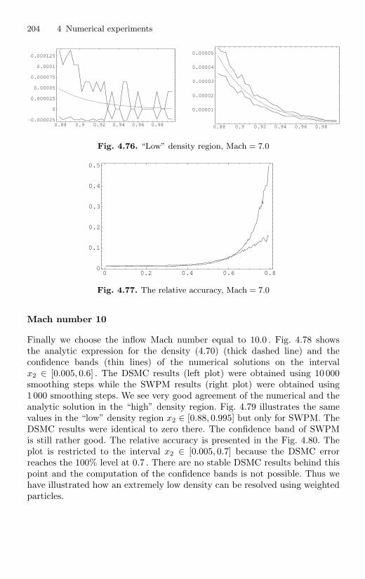
204 4 Numerical experiments
0.88 0.9 0.92 0.94 0.96 0.98-0.000025
0
0.000025
0.00005
0.000075
0.0001
0.000125
0.88 0.9 0.92 0.94 0.96 0.98
0.00001
0.00002
0.00003
0.00004
0.00005
Fig. 4.76. “Low” density region, Mach = 7.0
0 0.2 0.4 0.6 0.80
0.1
0.2
0.3
0.4
0.5
Fig. 4.77. The relative accuracy, Mach = 7.0
Mach number 10
Finally we choose the inflow Mach number equal to 10.0 . Fig. 4.78 showsthe analytic expression for the density (4.70) (thick dashed line) and theconfidence bands (thin lines) of the numerical solutions on the intervalx2 ∈ [0.005, 0.6] . The DSMC results (left plot) were obtained using 10 000smoothing steps while the SWPM results (right plot) were obtained using1 000 smoothing steps. We see very good agreement of the numerical and theanalytic solution in the “high” density region. Fig. 4.79 illustrates the samevalues in the “low” density region x2 ∈ [0.88, 0.995] but only for SWPM. TheDSMC results were identical to zero there. The confidence band of SWPMis still rather good. The relative accuracy is presented in the Fig. 4.80. Theplot is restricted to the interval x2 ∈ [0.005, 0.7] because the DSMC errorreaches the 100% level at 0.7 . There are no stable DSMC results behind thispoint and the computation of the confidence bands is not possible. Thus wehave illustrated how an extremely low density can be resolved using weightedparticles.

4.6 A spatially two-dimensional example 205
0 0.1 0.2 0.3 0.4 0.5 0.60
0.2
0.4
0.6
0.8
1
0 0.1 0.2 0.3 0.4 0.5 0.60
0.2
0.4
0.6
0.8
1
Fig. 4.78. “High” density region, Mach = 10.0
0.88 0.9 0.92 0.94 0.96 0.980
2.5�10-9
5�10-9
7.5�10-9
1�10-8
1.25�10-8
1.5�10-8
Fig. 4.79. “Low” density region, Mach = 10.0
0 0.1 0.2 0.3 0.4 0.5 0.6 0.70
0.2
0.4
0.6
0.8
1
Fig. 4.80. The relative accuracy, Mach = 10.0

206 4 Numerical experiments
4.6.2 Case with collisions
Here we assume absorption of particles on the top part of the boundary andconsider the Knudsen number Kn = 0.05 . In this case there is no analyticinformation available. In Fig. 4.81 we show the density profile on the wholeinterval x2 ∈ [0.005, 0.995] . Here the thick dashed line represents the courseof the analytic solution (4.70) (i.e. the situation for Kn = ∞) while the thinlines represent the confidence bands obtained using DSMC. These results cor-respond to the rather low inflow Mach number Mach = 1.0 to make thedeviation from the collisionless case visible. The difference becomes smallerfor higher Mach numbers.
0 0.2 0.4 0.6 0.8 1
0.15
0.2
0.25
0.3
0.35
Fig. 4.81. The course of the density, Mach = 1.0
It is clear that collisions reduce the effect of artificial particles generatedaccording to the auxiliary stream. On their way these particles collide andchange their velocities so that not all of them will reach the desired regionof low density. However, for a high Mach number, there is still considerableefficiency gain achieved by SWPM as the following examples show.
Mach number 7
First we choose the inflow Mach number in (4.62) equal to 7.0 . Fig. 4.82 showsthe confidence bands for DSMC (thin lines) and SWPM (thick lines). The leftplot shows the situation in the “high” density region x2 ∈ [0.005, 0.6] . Thelow density region x2 ∈ [0.88, 0.995] is presented in the right plot. Thus wesee a considerable advantage of SWPM when computing small functionals.

4.6 A spatially two-dimensional example 207
0 0.1 0.2 0.3 0.4 0.5 0.6
0.2
0.4
0.6
0.8
1
0.88 0.9 0.92 0.94 0.96 0.98
0
0.00002
0.00004
0.00006
0.00008
0.0001
0.00012
0.00014
Fig. 4.82. The course of the density, Mach = 7
Mach number 10
Now we choose the inflow Mach number equal to 10.0 . In this case no stableresults in the low density region x2 ∈ [0.88, 0.95] could be obtained usingDSMC, even with 10 times more computational time compared with SWPM.In this sense the situation is similar to the collisionless case. The numericalresults for SWPM are shown in Fig. 4.83. The empirical mean value of thedensity is represented with a thick dashed line while the thin lines correspondto the confidence bands. The left plot shows the situation in the “high” densityregion x2 ∈ [0.005, 0.6] . The low density region x2 ∈ [0.88, 0.995] is presentedin the right plot. The results obtained using SWPM are not as good as inthe collisionless case (there are some considerable fluctuations). However thesmall values of the density are resolved.
0 0.1 0.2 0.3 0.4 0.5 0.60
0.2
0.4
0.6
0.8
1
0.88 0.9 0.92 0.94 0.96 0.98-5�10-9
0
5�10-9
1�10-8
1.5�10-8
2�10-8
2.5�10-8
Fig. 4.83. The course of the density, Mach = 10
4.6.3 Influence of a hot wall
Here we assume diffuse reflection (1.38) of particles on the top part of theboundary, with a boundary Maxwellian
MΓt(v) =
12π (Tt)2
exp(− |v|2
2Tt
)

208 4 Numerical experiments
having constant temperature Tt = 300.0 . The inflow Mach number in (4.62)is chosen equal to 5.0 . The number of averaging time steps after reaching the“steady-state” situation was 10 000 .
We first consider the collisionless case. Figs. 4.84-4.87 show on the leftthe contour plots of the density, of the Mach number, of the temperatureand of the criteria of the local thermal equilibrium while the right plots showthe absolute values of these quantities plotted along the axis of symmetryx2 = 0 . The picture of the flow changes if we consider the Knudsen numberKn = 0.05 . The corresponding results are shown in Figs. 4.88–4.91. Now theinfluence of the hot top on the flow values at the left boundary is almostnegligible. Instead there is a clear maximum of the density in the middle ofthe domain. In the same region the temperature reaches its maximum.
0 50 100 150 2000
20
40
60
80
0 1 2 3 4
0.85
0.9
0.95
1
Fig. 4.84. Density, Kn = ∞
0 50 100 150 2000
20
40
60
80
0 1 2 3 4
3.2
3.4
3.6
3.8
4
Fig. 4.85. Mach number, Kn = ∞
0 50 100 150 2000
20
40
60
80
0 1 2 3 4
16
18
20
22
24
Fig. 4.86. Temperature, Kn = ∞

4.6 A spatially two-dimensional example 209
0 50 100 150 2000
20
40
60
80
0 1 2 3 4
1
1.5
2
2.5
3
3.5
Fig. 4.87. Criteria of local thermal equilibrium, Kn = ∞
0 50 100 150 2000
20
40
60
80
0 0.5 1 1.5 21
1.2
1.4
1.6
1.8
Fig. 4.88. Density, Kn = 0.05
0 50 100 150 2000
20
40
60
80
0 0.5 1 1.5 2
2
2.5
3
3.5
4
4.5
5
Fig. 4.89. Mach number, Kn = 0.05
0 50 100 150 2000
20
40
60
80
0 0.5 1 1.5 210
20
30
40
50
Fig. 4.90. Temperature, Kn = 0.05
0 50 100 150 2000
20
40
60
80
0 0.5 1 1.5 2
0.1
0.2
0.3
0.4
Fig. 4.91. Criteria of local thermal equilibrium, Kn = 0.05

210 4 Numerical experiments
4.6.4 Bibliographic remarks
The example considered in this section was motivated by the problem of su-personic molecular beam skimmers first studied in [22]. Further investigationsrelated to this problem can be found in [39]. The geometry of Fig. 4.71 wasconsidered in [181]. Though the example is extremely simplified, the resultsobtained so far are just a preliminary step.

A
Auxiliary results
A.1 Properties of the Maxwell distribution
Here we collect some analytic formulas for functionals of the Maxwell distri-bution. These functionals are expressed in terms of the following functions.The gamma function is defined as
Γ (s) =∫ ∞
0
xs−1 e−x dx , s > 0 , (A.1)
and has the properties
Γ (s) = (s − 1)Γ (s − 1) , s > 1 , (A.2)Γ (1) = 1 , Γ (0.5) =
√π .
The error function is defined as
erf(y) =2√π
∫ y
0
exp(−z2) dz , y ≥ 0 ,
erf(y) = −erf(−y) , y < 0 . (A.3)
It satisfies erf(∞) = 1 .
Lemma A.1. For any α > −3 , the following holds
G(α) :=∫
R3|v|α M0,1(v) dv =
2α+2
2
√π
Γ
(α + 3
2
). (A.4)
If α = 2n , n = 1, 2, . . . , then (A.4) takes the form
G(2n) =2n+1
√π
2n + 12
. . .12
Γ
(12
)=
n−1∏l=0
(3 + 2 l) .
In particular, one obtains
G(2) = 3 , G(4) = 15 , G(6) = 105 , G(8) = 945 . (A.5)

212 A Auxiliary results
Proof. Switching to spherical coordinates and using the substitution r =√2x , one obtains
G(α) =∫ ∞
0
rα 1(2π)3/2
exp(−r2/2) r2 (4π) dr
= 2−32+2+ α+2
2 − 12 π− 3
2+1
∫ ∞
0
xα+1
2 e−x dx
so that (A.4) follows from (A.1).Further moments of the Maxwell distribution are∫
R3|v|α M0,T (v) dv = Tα/2 G(α) , (A.6)
and ∫R3
vvT MV,T (v) dv = T I + V V T , (A.7a)
∫R3
v|v|2 MV,T (v) dv = (5T + |V |2)V , (A.7b)
∫R3
|v|4 MV,T (v) dv = |V |4 + 15T 2 + 10T |V |2 . (A.7c)
Lemma A.2. For any e ∈ S2 , the following holds∫(v,e)>0
MV,T (v) (v, e) dv = (A.8)
√T
2πexp
(−(V, e)2
2T
)+
(V, e)2
[1 + erf
((V, e)√
2T
)].
If (V, e) = 0 , then (A.8) takes the form
∫(v,e)>0
MV,T (v) (v, e) dv =
√T
2π
and the appropriate normalization factor is
1(2πT )3/2
√2π
T=
12πT 2
.
Proof. Using the substitution
v = V +√
2T v , dv = (2T )3/2dv
as well as a rotation of the coordinate system such that e becomes the firstbasis vector, one obtains
A.2 Exact relaxation of moments 213∫(v,e)>0
MV,T (v) (v, e) dv =√
2T
π3/2
∫(v,e)>−a
[a + (v, e)
]exp(−|v|2)dv
=√
2T
π3/2
∫ξ1>−a
(a + ξ1) exp(−ξ21)dξ1
∫R2
exp(−ξ22 − ξ2
3)dξ2 dξ3 (A.9)
=
√2T
π
a∫−∞
(a − z) exp(−z2) dz , where a =(V, e)√
2T.
Sincey∫
−∞(a − z) exp(−z2) dz = a
√π
2
[1 + erf(y)
]+
12
exp(−y2) , (A.10)
for any y ≤ a , assertion (A.8) follows from (A.9).Finally, tails of the Maxwell distribution take the form (cf. (A.3))
TailV,T (U,R) :=∫
|v−U |≥R
MV,T (v) dv (A.11)
= 1 +12
(erf(a − b√
2
)− erf
(a + b√2
))+
1√2π a
(exp(− (a − b)2
2
)− exp
(− (a + b)2
2
)),
where
a =|V − U |√
T, b =
R√T
.
If the tail functional is centered, i.e. U = V , then one obtains
(A.12)
TailV,T (V,R) = limU→V
TailV,T (U,R) = 1 − erf( b√
2
)+
2√π
b exp(− b2
2
).
A.2 Exact relaxation of moments
Here we consider the spatially homogeneous Boltzmann equation (4.1) withconstant collision kernel (4.3). Following the paper [33], we find analytic ex-pressions for the relaxation of the moments (4.8a)-(4.8c) of the solution. Weuse the notations (4.5)-(4.7) and assume = 1 .

214 A Auxiliary results
Lemma A.3. The moments (4.8a)-(4.8c) satisfy the system of ordinary dif-ferential equations (cf. (1.89))
d
dtM(t) = −1
2M(t) +
12
(T I + V V T
), (A.13a)
d
dtr(t) = −1
3r(t) +
23
(3T + |V |2
)V − 1
3M(t)V , (A.13b)
d
dts(t) = −1
3s(t) +
23
(3T + |V |2
)2− 1
3||M(t)||2F . (A.13c)
Proof. The derivation uses the weak form of the Boltzmann collision inte-gral (cf. Lemma 1.11)∫
R3
g(v)Q(f, f)(v) dv = (A.14)
12
∫R3
∫R3
f(v)f(w)14π
∫S2
(g(v′) + g(w′) − g(v) − g(w)
)de dw dv ,
where Q(f, f)(v) denotes the right-hand side of equation (4.1) and v′, w′ arethe post-collision velocities (1.6). First we consider the test function g(v) =vvT . Using the property
14π
∫S2
eeT de =13
I
we compute the average over the unit sphere in (A.14) and obtain
14π
∫S2
(v′(v′)T + w′(w′)T − vvT − wwT
)de =
−12
(vvT + wwT + vwT + wvT
)+
16
(|v|2 + |w|2 − 2(v, w)
)I .
The conservation property∫R3
|v|2f(t, v) dv = 3T + |V |2
implies then ∫R3
vvTQ(f, f)(v) dv = −12M(t) +
12
(T I + V V T
). (A.15)
Averaging g(v) = v|v|2 over the unit sphere leads to

A.2 Exact relaxation of moments 215
14π
∫S2
(v′|v′|2 + w′|w′|2 − v|v|2 − w|w|2
)de =
−13
(v|v|2 + w|w|2 + (v, w)(v + w)
)+
23
(v|w|2 + w|v|2
)and ∫
R3
v|v|2Q(f, f)(v) dv = −13r(t) +
23
(3T + |V |2
)V − 1
3M(t)V . (A.16)
Finally, using the test function g(v) = |v|4 gives
14π
∫S2
(|v′|4 + |w′|4 − |v|4 − |w|4
)de =
−13
(|v|4 + |w|4 + 2(v, w)2
)+
43|v|2|w|2
and ∫R3
|v|4Q(f, f)(v) dv = −13s(t) +
23
(3T + |V |2
)2− 1
3||M(t)||2F . (A.17)
The assertion follows from the Boltzmann equation and the properties (A.15)-(A.17).
The linear system (A.13a)-(A.13c) can be solved explicitly and the solutiontakes the form
M(t) = M0 e−t/2 +(T I + V V T
)(1 − e−t/2
), (A.18a)
r(t) = r0 e−t/3 +(5T + |V |2
)V(1 − e−t/3
)(A.18b)
+2(M0 − V V T − T I
)V(e−t/2 − e−t/3
),
s(t) = s0 e−t/3 +(|V |4 + 15T 2 + 10T |V |2
)(1 − e−t/3
)(A.18c)
+12
(||M0||2F − 3T 2 + |V |4 − 2(M0V, V )
)(e−t − e−t/3
)+4((M0V, V ) − |V |4 − T |V |2
)(e−t/2 − e−t/3
),
where
M0 =∫R3
vvT f0(v) dv , r0 =∫R3
v|v|2 f0(v) dv , s0 =∫R3
|v|4 f0(v) dv
are the corresponding moments of the initial distribution f0 of the Boltzmannequation. Formulas (A.18a)-(A.18c) are extremely useful for numerical tests

216 A Auxiliary results
because they provide the explicit time evolution of moments of the solution ofthe Boltzmann equation for any initial condition. Furthermore, they allow usto obtain an analytic expression for the function (4.9) representing a criterionfor thermal local equilibrium. The terms (4.10a)-(4.10c) satisfy
τ(t) = M(t) −(V V T + T I
), (A.19)
q(t) =12
(r(t) − 2M(t)V + |V |2 V − 3T V
)=
12
(r(t) − (5T + |V |2)V
)− τ(t)V (A.20)
and
γ(t) =∫R3
|v − V |2 |v|2 f(t, v) dv − 3T |V |2 − 4 (q(t), V ) − 15T 2
= s(t) − 2 (r(t), V ) + |V |2(3T + |V |2
)− 3T |V |2 − 4 (q(t), V ) − 15T 2
= s(t) −(|V |4 + 15T 2 + 10T |V |2
)− 4 (τ(t)V, V ) − 8 (q(t), V ) . (A.21)
Note that w (v, V ) = w vT V and |v−V |2 = |v|2−|V |2−2(v−V, V ) . Accordingto (A.18a)-(A.18c), we conclude from (A.19)-(A.21) that
τ(t) =(M0 − V V T − T I
)e−t/2 , (A.22)
q(t) =12
(r0 − (5T + |V |2)V
)e−t/3+(
M0 − V V T − T I)
V(e−t/2 − e−t/3
)−(M0 − V V T − T I
)V e−t/2
=12
(r0 − 2M0V + (|V |2 − 3T )V
)e−t/3 (A.23)
and
γ(t) =(s0 − |V |4 − 15T 2 − 10T |V |2
)e−t/3 +
12
(||M0||2F − 3T 2 + |V |4 − 2 (M0V, V )
)(e−t − e−t/3
)+
4((M0V, V ) − |V |4 − T |V |2
)(e−t/2 − e−t/3
)−
4((M0V, V ) − |V |4 − T |V |2
)e−t/2 −
4((r0, V ) − 2 (M0V, V ) + (|V |2 − 3T ) |V |2
)e−t/3
=12
(2 s0 − 3 |V |4 − 27T 2 + 12T |V |2 − ||M0||2F +

A.3 Properties of the BKW solution 217
10 (M0V, V ) − 8 (r0, V ))e−t/3 + (A.24)
12
(||M0||2F − 3T 2 + |V |4 − 2 (M0V, V )
)e−t .
A.3 Properties of the BKW solution
Here we consider the spatially homogeneous Boltzmann equation (4.1) withthe collision kernel
B(v, w, e) = B(cos(θ)) , cos(θ) =(v − w, e)|v − w| ,
where ∫S2
B
((v − w, e)|v − w|
)de < ∞ ,
and study the famous exact solution found by Bobylev [27] and Krook andWu [115]. We look for a solution in the form
f(t, v) =(a + b|v|2
)e−c|v|2 , (A.25)
where the parameters a, b and c are functions of the time variable t . Since thebulk velocity satisfies V (t) = 0 by symmetry, there are only two conservedphysical quantities of the solution (A.25), namely the density (t) and thetemperature T (t) . This fact provides two equations for the unknown parame-ters a, b, c . Using the substitution
√2c w = w′ one obtains (cf. (A.4), (A.5))
∫R3
e−c|w|2dw =1
(2c)3/2(2π)3/2 G(0) = π3/2 1
c3/2,
∫R3
|w|2e−c|w|2dw =1
(2c)5/2(2π)3/2 G(2) =
3π3/2
21
c5/2,
∫R3
|w|4e−c|w|2dw =1
(2c)7/2(2π)3/2 G(4) =
15π3/2
41
c7/2
so that
(t) =∫R3
f(t, v) dv =π3/2
22ac + 3b
c5/2= (A.27)
and

218 A Auxiliary results
3 T (t) =∫R3
|v|2 f(t, v) dv =π3/2
42ac + 5b
c7/2= 3 T . (A.28)
Using (A.27) and (A.28), we express the functions a and b in terms of , Tand c ,
a =1
π3/2 c3/2(5/2 − 3Tc) , b =
1π3/2
c5/2(2Tc − 1) , (A.29)
so that the function (A.25) takes the form
f(t, v) =
π3/2
(2T |v|2c7/2 − (3T + |v|2)c5/2 + 5/2c3/2
)e−c|v|2 . (A.30)
Next we use the Boltzmann equation (4.1) to determine the remainingparameter c . The time derivative of the function (A.30) is
∂
∂tf =
π3/2c1/2(1 − 2Tc)
(c2|v|4 − 5c|v|2 + 15/4
)e−c|v|2 dc
dt. (A.31)
We denote the right-hand side of equation (4.1) by Q(f, f) and compute thiscollision integral for the function (A.25). First, using conservation of energyduring a collision, we get
f(v′)f(w′) − f(v)f(w) = b2(|v′|2|w′|2 − |v|2|w|2
)e−c(|v|2 + |w|2
).
Then, with the substitutions
U =12(v + w
), u = v − w ,
we obtain
|v′|2|w′|2 − |v|2|w|2 = (U, u)2 − |u|2(U, e)2 = (U, u)2 − |u|2UTeeTU .
Thus the integral over the unit sphere leads to
e−c(|v|2 + |w|2
) ∫S2
B
((u, e)|u|
)((U, u)2 − |u|2UTeeTU
)de .
This integral can be computed using spherical coordinates related to the di-rection of the vector u . The result is
α e−c(|v|2 + |w|2
)(3(U, u)2 − |u|2|U |2
)=
α
2e−c(|v|2 + |w|2
)(|v|4 + |w|4 − 4|v|2|w|2 + 2vT wwT v
),
where

A.3 Properties of the BKW solution 219
α = π
π∫0
B(cos θ) sin3 θ dθ . (A.32)
Integrating the last expression with respect to w over R3 we get the final
result
Q(f, f) = b2 α
2π3/2 1
c7/2
(c2|v|4 − 5c|v|2 + 15/4
)e−c|v|2 . (A.33)
Equating (A.31) and (A.33) and using (A.29), one obtains the differentialequation for the function c
dc
dt= −α
2 (2Tc − 1) c .
Using the substitution 2Tc − 1 = β we get
dβ
dt= −α
2 β (β + 1)
and finally
β(t) =β0 e−α � t/2
1 + β0 (1 − e−α � t/2), (A.34)
where β0 denotes the initial value for the function β and α is defined in (A.32).Putting c = (β + 1)/(2T ) into (A.30) we obtain
f(t, v) = (A.35)
(2πT )3/2(β(t) + 1)3/2
(1 + β(t)
(β(t) + 12T
|v|2 − 32
))e−
β(t)+12T |v|2 .
This solution is non-negative for
0 ≤ β0 ≤ 2/3 . (A.36)
In the following we derive explicit expressions for certain functionals ofthe solution (A.35), which are useful for numerical tests. We assume = 1 .Introducing the notation Tβ = T/(β + 1) and taking into account (A.6) and(A.4), one obtains∫
R3
|v|α f(t, v) dv =
(1 − 3
2β
)∫R3
|v|α M0,Tβ(v) dv +
β
2Tβ
∫R3
|v|α+2 M0,Tβ(v) dv
=(
1 − 32
β
)T
α2
β
2α+2
2
√π
Γ
(α + 3
2
)+
β
2TβT
α+22
β
2α+4
2
√π
Γ
(α + 5
2
)
=1√π
(2Tβ)α2 Γ
(α + 3
2
)(2 − 3β + β(α + 3)
).

220 A Auxiliary results
Thus, power functionals of the solution (A.35) take the form∫R3
|v|α f(t, v) dv =1√π
(2T )α/2 Γ(α + 3
2
) α β + 2(β + 1)α/2
,
where α > −3 and β = β(t) is defined in (A.34). If α = m ∈ N then oneobtains using (A.2)
∫R3
|v|m f(t, v) dv =
⎧⎪⎪⎪⎨⎪⎪⎪⎩
1√π
(k + 1
)!(
β + 12T
)−m/2(mβ + 2
), m = 2 k + 1 ,
(2 k + 1
)!!(
β + 1T
)−k(k β + 1
), m = 2 k .
(A.37)
Furthermore, we derive an analytic expression for the function (4.9) repre-senting a criterion of local thermal equilibrium. Since by symmetry (cf. (4.8a)-(4.8c)) V = 0 , M(t) = T I , r(t) = 0 and according to (A.37)
s(t) =∫R3
|v|4 f(t, v) dv = 15T 2 2β + 1(β + 1)2
,
the terms (4.10a)-(4.10c) satisfy
τ(t) = 0 , q(t) = 0 , γ(t) = −15T 2
(β
β + 1
)2
so that the function (4.9) takes the form
Crit(t) =
√158
(β
β + 1
)2
. (A.38)
Finally, tail functionals (4.11) of the solution (A.35) take the form (cf. (A.3)),
Tail(R, t) = (A.39)
1 +2√π
√β + 12T
R(1 + βR2 β + 1
2T
)exp(− β + 1
2TR2)− erf
(√β + 12T
R).
A.4 Convergence of random measures
Here we collect some convergence properties of random measures. We considerthe space Z = D × R
3 and the metric L defined in (3.153). Let ν(n) be asequence of random measures such that
ν(n)(Z) ≤ C a.s. (A.40)
and ν be a deterministic finite measure on Z .
A.4 Convergence of random measures 221
Lemma A.4. The following conditions are equivalent:
(i) limn→∞ E L(ν(n), ν) = 0
(ii) L(ν(n), ν) → 0 in probability(iii) 〈ϕ, ν(n)〉 → 〈ϕ, ν〉 in probability,
for any continuous bounded function ϕ
(iv) 〈ϕ, ν(n)〉 → 〈ϕ, ν〉 in probability,for any measurable bounded function ϕ such that ν(D(ϕ)) = 0 ,
where D(ϕ) denotes the set of discontinuity points of the function ϕ .
Lemma A.4 was proved in [204, Cor. 3.5].
Corollary A.5 Let the measure ν be absolutely continuous with respect toLebesgue measure. Then the following conditions are equivalent:
(i) L(ν(n), ν) → 0 in probability
(ii) L(ν(n)l , νl) → 0 in probability, ∀ l = 1, . . . , lc ,
where ν(n)l , νl denote the restrictions of the measures ν(n), ν to the sets Dl×R
3
(cf. (3.58)).
Lemma A.6. Let ξn be a sequence of random variables. If
limn→∞ E ξn = a ∈ (−∞,∞) and lim
n→∞Var ξn = 0 (A.41)
then
ξn → a in probability. (A.42)
If
supn
|ξn| ≤ c < ∞ a.s.
then (A.42) implies (A.41).
Proof. The first assertion follows from
Prob(|ξn − a| ≥ ε) ≤ Prob(|ξn − E ξn| + |E ξn − a| ≥ ε)
≤ Prob(|ξn − E ξn| ≥ ε/2) ≤ 2Var ξn
ε,
where ε > 0 is arbitrary and n is sufficiently large. The estimates
|E ξn − a| ≤ E |ξn − a| ≤ (a + c) Prob(|ξn − a| > ε) + ε
and
Var ξn = E (ξn − a)2 − (E ξn − a)2
≤ (a + c)2 Prob(|ξn − a| > ε) + ε2 − (E ξn − a)2
imply the second assertion.

222 A Auxiliary results
Lemma A.7. Let the measure ν be absolutely continuous with respect toLebesgue measure. If
L(ν(n), ν) → 0 in probability (A.43)
then ∫Z
∫Z
Φ(z, z1) ν(n)(dz) ν(n)(dz1) →∫Z
∫Z
Φ(z, z1) ν(dz) ν(dz1) in probability,
for any continuous bounded function Φ .
Proof. Consider a step function
ΦN (z, z1) =kN∑i=1
cN,iχAN,i(z)χBN,i
(z1) ,
where N ≥ 1 , kN ≥ 1 and AN,i, BN,i are rectangles in Z . Denote
a(n) =∣∣∣∣∫
Z
∫Z
Φ(z, z1) ν(n)(dz) ν(n)(dz1) −∫
Z
∫Z
Φ(z, z1) ν(dz) ν(dz1)∣∣∣∣
and
b(n)R,N =∣∣∣∣∫
ZR
∫ZR
ΦN (z, z1) ν(n)(dz) ν(n)(dz1) −∫
ZR
∫ZR
ΦN (z, z1) ν(dz) ν(dz1)∣∣∣∣ ,
where
ZR = {z ∈ Z : |z| ≤ R} , R > 0 .
Using (A.43), (A.40), absolute continuity of ν , Lemma A.4 and Lemma A.6,one obtains
limn→∞ E b
(n)R,N = 0 , ∀R,N , (A.44)
and ν(Z) ≤ C . The triangle inequality implies
a(n) ≤∣∣∣∣∫
Z
∫Z
Φ(z, z1) ν(n)(dz) ν(n)(dz1) −∫
ZR
∫ZR
Φ(z, z1) ν(n)(dz) ν(n)(dz1)∣∣∣∣+∣∣∣∣
∫ZR
∫ZR
Φ(z, z1) ν(n)(dz) ν(n)(dz1)−
A.5 Existence of solutions 223∫ZR
∫ZR
ΦN (z, z1) ν(n)(dz) ν(n)(dz1)∣∣∣∣+ b
(n)R,N +∣∣∣∣
∫ZR
∫ZR
ΦN (z, z1) ν(dz) ν(dz1) −∫
ZR
∫ZR
Φ(z, z1) ν(dz) ν(dz1)∣∣∣∣+∣∣∣∣
∫ZR
∫ZR
Φ(z, z1) ν(dz) ν(dz1) −∫
Z
∫Z
Φ(z, z1) ν(dz) ν(dz1)∣∣∣∣
≤ 2C ||Φ||∞ ν(n)(Z \ ZR) + C2 sup(z,z1)∈ZR×ZR
|Φ(z, z1) − ΦN (z, z1)| + b(n)R,N +
C2 sup(z,z1)∈ZR×ZR
|Φ(z, z1) − ΦN (z, z1)| + 2C ||Φ||∞ ν(Z \ ZR) , (A.45)
for any R and N . Consider the measures ν(n) defined as
ν(n)(B) = E ν(n)(B) , B ∈ B(Z) ,
and note that 〈ϕ, ν(n)〉 = E 〈ϕ, ν(n)〉 . Using (A.40), (A.43), Lemma A.4 andLemma A.6, one obtains that the measures ν(n) converge weakly to the mea-sure ν . Tightness implies that, for any ε > 0 , there exists R such that
supn
ν(n)(Z \ ZR) ≤ ε and ν(Z \ ZR) ≤ ε . (A.46)
For given ε and R , there exists a step function ΦN such that
sup(z,z1)∈ZR×ZR
|Φ(z, z1) − ΦN (z, z1)| ≤ ε , (A.47)
since Φ is continuous. Using (A.46) and (A.47) one obtains from (A.45) that
E a(n) ≤ 4C ||Φ||∞ ε + 2C2ε + E b(n)R,N
and, according to (A.44),
lim supn→∞
E a(n) ≤ 4C ||Φ||∞ ε + 2C2ε , ∀ ε > 0 ,
so that the assertion follows.
A.5 Existence of solutions
Existence results for the spatially homogeneous or the mollified Boltzmannequation can be found in [4], [48, Ch. VIII.2]. For completeness, we reproducea version adapted to our purpose (cf. Remark 3.26).
Theorem A.8. Let the mollifying function h and the collision kernel B sat-isfy (3.149) and f0 be such that
f0(x, v) ≥ 0 (A.48)

224 A Auxiliary results
and
||f0||1 =∫
D
∫R3
f0(x, v) dv dx < ∞ . (A.49)
Then there exists a unique solution in L1(D × R3) of the equation
∂
∂tf(t, x, v) =
∫D
∫R3
∫S2
h(x, y)B(v, w, e)× (A.50)[f(t, x, v′) f(t, y, w′) − f(t, x, v) f(t, y, w)
]de dw dy
with the initial condition
f(0, x, v) = f0(x, v) . (A.51)
This solution satisfies
f(t, x, v) ≥ 0 , t ≥ 0 , (A.52)
and ∫D
∫R3
f(t, x, v) dv dx =∫
D
∫R3
f0(x, v) dv dx . (A.53)
If, in addition, ∫D
∫R3
|v|2 f0(x, v) dv dx < ∞ (A.54)
then ∫D
∫R3
|v|2 f(t, x, v) dv dx =∫
D
∫R3
|v|2 f0(x, v) dv dx . (A.55)
Remark A.9. The corresponding measure-valued function
F (t, dx, dv) = f(t, x, v) dx dv
solves the weak equation (3.168). �
Introduce the operators
Q1(f)(x, v) =∫
D
∫R3
∫S2
h(x, y)B(v, w, e) f(y, w) de dw dy
and
Q2(f, g)(x, v) =∫
D
∫R3
∫S2
h(x, y)B(v, w, e) f(x, v′) g(y, w′) de dw dy ,
where f, g ∈ L1(D × R3) . Equation (A.50), (A.51) takes the form
A.5 Existence of solutions 225
d
dtf(t) = Q(f(t), f(t)) , f(0) = f0 , (A.56)
where
Q(f, g) = Q2(f, g) − f Q1(g) . (A.57)
Using properties of the mollifying function h , the collision kernel B and thecollision transformation v′, w′ , one obtains (cf. Lemma 1.3 and (1.55))∫
D
∫R3
Q2(f, g)(x, v) dv dx =∫
D
∫R3
f(x, v)Q1(g)(x, v) dv dx (A.58)
and ∫D
∫R3
|v|2 Q2(f, f)(x, v) dv dx =12
∫D
∫R3
∫D
∫R3
∫S2[
|v′|2 + |w′|2]h(x, y)B(v, w, e) f(x, v) f(y, w) de dw dy dv dx
=∫
D
∫R3
|v|2 f(x, v)Q1(f)(x, v) dv dx , (A.59)
for non-negative f, g . Assumption (3.149) implies
|Q1(f)(x, v)| ≤ Cb ||f ||1 (A.60)
so that
||Q2(f, g)||1 ≤ Cb ||f ||1 ||g||1 (A.61)
and∫D
∫R3
|v|2 Q2(f, f)(x, v) dv dx ≤ Cb ||f ||1∫
D
∫R3
|v|2 f(x, v) dv dx , (A.62)
according to (A.58) and (A.59).
Lemma A.10. Consider the iteration scheme
fn+1(t) = exp(−c t ||f0||1) f0 +∫ t
0
exp(−c (t − s) ||f0||1) × (A.63)(Q2(fn(s), fn(s)) + fn(s)
[c ||fn(s)||1 − Q1(fn(s))
])ds ,
f0(t) = 0 , t ≥ 0 , n = 0, 1, 2, . . . , c ≥ Cb ,
where f0 satisfies (A.48), (A.49). Then, for any n = 1, 2, . . . and t ≥ 0 ,
fn(t, x, v) ≥ fn−1(t, x, v) ≥ 0 , (A.64)
||fn(t)||1 ≤ ||f0||1 (A.65)
and ∫D
∫R3
|v|2 fn(t, x, v) dv dx ≤∫
D
∫R3
|v|2 f0(x, v) dv dx . (A.66)

226 A Auxiliary results
Proof. Properties (A.64)-(A.66) are fulfilled for n = 1 , according to defin-ition (A.63). Assume these properties hold for some n ≥ 1 . Using (A.64),
Q2(fn(s), fn(s)) ≥ Q2(fn−1(s), fn−1(s))
and (cf. (A.60))
c ||fn(s)||1 − Q1(fn(s)) = c ||fn(s) − fn−1(s)||1−Q1(fn(s) − fn−1(s)) + c ||fn−1(s)||1 − Q1(fn−1(s))
≥ c ||fn−1(s)||1 − Q1(fn−1(s)) ,
one obtains
fn+1(t, x, v) ≥ fn(t, x, v) . (A.67)
According to (A.58), definition (A.63) implies
||fn+1(t)||1 = (A.68)
exp(−c t ||f0||1) ||f0||1 + c
∫ t
0
exp(−c (t − s) ||f0||1) ||fn(s)||21 ds .
Using (A.65) one obtains
||fn+1(t)||1 ≤ (A.69)
exp(−c t ||f0||1) ||f0||1 + c ||f0||21∫ t
0
exp(−c (t − s) ||f0||1) ds = ||f0||1 .
Finally, (A.63), (A.59), (A.65) and (A.66) imply∫D
∫R3
|v|2 fn+1(t, x, v) dv dx ≤ exp(−c t ||f0||1)∫
D
∫R3
|v|2 f0(x, v) dv dx +
c ||f0||1∫
D
∫R3
|v|2 f0(x, v) dv dx
∫ t
0
exp(−c (t − s) ||f0||1) ds
=∫
D
∫R3
|v|2 f0(x, v) dv dx . (A.70)
Thus, taking into account (A.67), (A.69) and (A.70), the assertions follow byinduction.Proof of Theorem A.8. By Lemma A.10 and the monotone convergencetheorem there exists
f(t) = limn→∞ fn(t) in L1(D × R
3) , t ≥ 0 .
By continuity of the operators (cf. (A.60), (A.61)), this limit f(t) satisfies (cf.(A.63))
A.5 Existence of solutions 227
f(t) = exp(−c t ||f0||1) f0 + (A.71)∫ t
0
exp(−c (t − s) ||f0||1)(Q2(f(s), f(s)) + f(s)
[c ||f(s)||1 − Q1(f(s))
])ds
and β(t) := ||f(t)||1 satisfies (cf. (A.68))
β(t) = exp(−c t ||f0||1) ||f0||1 + c
∫ t
0
exp(−c (t − s) ||f0||1)β(s)2 ds . (A.72)
Note that β0(t) := ||f0||1 is the unique solution of equation (A.72). Thus,equation (A.71) takes the form
f(t) = exp(−c t ||f0||1) f0 + (A.73)∫ t
0
exp(−c (t − s) ||f0||1)(Q2(f(s), f(s)) + f(s)
[c ||f0||1 − Q1(f(s))
])ds .
A differentiation in (A.73) implies that f(t) satisfies (A.56). Moreover, (A.52)and (A.53) are fulfilled.
Using (A.66) and the monotone convergence theorem, one obtains∫D
∫R3
|v|2 f(t, x, v) dv dx ≤∫
D
∫R3
|v|2 f0(x, v) dv dx . (A.74)
Finally, it follows from (A.59) that (cf. (A.60)-(A.62), (A.54))∫D
∫R3
|v|2 Q(f, f)(x, v) dv dx = 0 ,
and (A.56) implies equality in (A.74) so that (A.55) holds.Uniqueness follows from the local Lipschitz property of the operator (A.57)
(cf. (A.60), (A.61)),
||Q(f, f) − Q(g, g)||1 ≤ Cb ||f − g||1[||f ||1 + ||g||1
].
This completes the proof.

B
Modeling of distributions
Here we collect some material concerning the generation of samples from agiven distribution. In particular, we describe all procedures used in the nu-merical experiments of Chapter 4. Alternative (sometimes more efficient) al-gorithms can be found in Monte Carlo textbooks.
B.1 General techniques
B.1.1 Acceptance-rejection method
Consider some measurable space (X,µ) and two functions f and F on Xsatisfying the majorant condition
0 ≤ f(x) ≤ F (x) , ∀x ∈ X . (B.1)
Assume that ∫X
f(x)µ(dx) > 0 and∫
X
F (x)µ(dx) < ∞ .
Let a random variable ξ be defined by the following procedure:
1. Generate a random variable η with the probability density
P (x) =F (x)∫
XF (x)µ(dx)
. (B.2)
2. Generate independently a random variable u uniformly distributed on[0, 1] .
3. If the acceptance condition
u ≤ f(η)F (η)
(B.3)
is satisfied, then ξ = η and stop. Otherwise, go to 1.

230 B Modeling of distributions
Then the random variable ξ has the probability density
p(x) =f(x)∫
Xf(x)µ(dx)
.
The acceptance rate is ∫X
f(x)µ(dx)∫X
F (x)µ(dx).
B.1.2 Transformation method
Consider a random variable ξ with values in an open set G ⊂ Rd and density
pξ . Define the random variable
η = Φ−1(ξ) , (B.4)
where Φ : G1 → G is some diffeomorphism and G1 ⊂ Rd . One obtains
E f(η) = E f(Φ−1(ξ)) =∫
G
f(Φ−1(x)) pξ(x) dx
=∫
G1
f(y) pξ(Φ(y)) |det Φ′(y)| dy ,
where Φ′ denotes the Jacobian matrix and f is some test function. Conse-quently, the random variable (B.4) has the density
pη(y) = pξ(Φ(y)) |det(Φ′(y)| . (B.5)
Samples of ξ can be obtained by first generating η and then transforming theresult into ξ = Φ(η) .
Analogous arguments apply to the parametrization of ξ by spherical coor-dinates.
A simple particular case is (for strictly positive densities)
Φ = F−1ξ : (0, 1) → R ,
where Fξ denotes the distribution function of the random variable ξ . Thedensity (B.5) takes the form
pη(y) = pξ(F−1ξ (y))
1F ′
ξ(F−1ξ (y))
= 1 .
Thus, samples of ξ are obtained as
ξ = F−1ξ (η) ,
where η is uniformly distributed on [0, 1] .
B.2 Uniform distribution on the unit sphere 231
B.1.3 Composition method
Consider some probability space (Y, ν) and a family of probability measures
µy(dx) , y ∈ Y ,
on some measurable space X . Let a random variable ξ be defined by thefollowing procedure:
1. Generate a random variable η with values in Y according to ν .2. Generate ξ according to µη .
Then the random variable ξ has the distribution
P (dx) =∫
Y
µy(dx) ν(dy) . (B.6)
B.2 Uniform distribution on the unit sphere
Here we generate a random variable ξ according to the probability density
pξ(e) =1
4π, e ∈ S2 .
We apply the transformation method (cf. Section B.1.2).Switching to spherical coordinates
e = e(ϕ, θ) =
⎛⎝ cos ϕ sin θ
sin ϕ sin θcos θ
⎞⎠ , 0 ≤ ϕ < 2π , 0 ≤ θ ≤ π , (B.7)
one obtains
pη(ϕ, θ) =1
4πsin θ .
The components ϕ and θ of the random variable η are independent so that itremains to solve the equations
12π
ϕ∗∫0
dϕ = r1 ,12
θ∗∫0
sin θ dθ = r2 ,
where r1 and r2 are random numbers uniformly distributed on (0, 1) . Oneobtains
ϕ∗ = 2π r1 , cos θ∗ = 1 − 2 r2
and, according to (B.7),
ξ = e(ϕ∗, θ∗) . (B.8)

232 B Modeling of distributions
Algorithm B.1 Uniform distribution on the unit sphere
UniSphere(r1, r2)
1. Compute:ϕ∗ = 2π r1
2. Compute:cos θ∗ = 1 − 2 r2
3. Compute:
sin θ∗ =√
1 − (cos θ∗)2
4. Final result: (B.8)
B.3 Directed distribution on the unit sphere
Here we generate a random variable ξ according to the probability density
pξ(e) =1
2π|(u, e)| , e ∈ S2 ,
where u ∈ S2 is some parameter. We apply the transformation method (cf.Section B.1.2).
First we construct an orthogonal matrix Q(u) such that
Q(u)′ u = (0, 0, 1) ,
where Q′ denotes the transposed matrix. Note that the matrices
A1(ψ) =
⎛⎝1 0 0
0 cos ψ − sin ψ0 sin ψ cos ψ
⎞⎠ A2(ψ) =
⎛⎝ cos ψ 0 sin ψ
0 1 0− sin ψ 0 cos ψ
⎞⎠
A3(ψ) =
⎛⎝ cos ψ − sin ψ 0
sin ψ cos ψ 00 0 1
⎞⎠
perform rotations over an angle ψ around the first, second and third basisvectors, respectively. Let u be given in spherical coordinates as
u =(
cos ϕu sin θu , sin ϕu sin θu , cos(θu)).
Then one obtains
A3(−ϕu)u = u = (sin θu, 0, cos θu) , A2(−θu) u = (0, 0, 1)
so that Q(u)′ = A2(−θu)A3(−ϕu) and
B.3 Directed distribution on the unit sphere 233
Q(u) = A3(ϕu)A2(θu) =
⎛⎝ cos ϕu cos θu − sin ϕu cos ϕu sin θu
sin ϕu cos θu cos ϕu sin ϕu sin θu
− sin θu 0 cos θu
⎞⎠ . (B.9)
If sin θu = 0 then ϕu is not uniquely determined and it is convenient to putϕu = 0 .
Using the substitution (cf. (B.7))
e = Q(u) e(ϕ, θ) , 0 ≤ ϕ < 2π , 0 ≤ θ ≤ π , (B.10)
which corresponds to a rotation and a transition to spherical coordinates, oneobtains
pη(ϕ, θ) =1
2π|(u,Q(u) e(ϕ, θ))| sin θ
=1
2π|(Q(u)′u, e(ϕ, θ))| sin θ =
12π
| cos θ| sin θ .
Note that the uniform surface measure on the unit sphere is invariant withrespect to rotations. The components ϕ and θ of the random variable η areindependent so that it remains to solve the equations
12π
ϕ∗∫0
dϕ = r1 ,
θ∗∫0
| cos θ| sin θ dθ = r2 ,
where r1 and r2 are random numbers uniformly distributed on (0, 1) . Oneobtains
ϕ∗ = 2π r1 , cos θ∗ =
⎧⎨⎩
√1 − 2 r2 if r2 ≤ 1/2 ,
−√
2 r2 − 1 if r2 > 1/2 ,
and, according to (B.10),
ξ = Q(u) e(ϕ∗, θ∗) . (B.11)
Algorithm B.2 Directed distribution on the unit sphere
DirectUniSphere(r1, r2, u)
1. Compute:ϕ∗ = 2π r1
2. if r2 ≤ 1/2 then set
cos θ∗ =√
1 − 2 r2
else setcos θ∗ = −
√2 r2 − 1

234 B Modeling of distributions
3. Compute:
sin θ∗ =√
1 − (cos θ∗)2
4. If u = (0, 0, 1) or u = (0, 0,−1) , i.e. sin θu = 0 , then set
ϕu = 0
else compute
cos θu = u3 , sin θu =√
1 − cos2 θu ,
cos ϕu = u1/ sin θu , sin ϕu = u2/ sin θu
5. Final result: (B.11)
B.4 Maxwell distribution
Here we generate a random variable ξ according to the probability density
pξ(v) = MV,T (v) , v ∈ R3 . (B.12)
We apply the transformation method (cf. Section B.1.2).Using the substitution
v = V +√
T w , dv = T 3/2 dw (B.13)
and switching to the spherical coordinates
w = r e , 0 ≤ r < ∞ , e ∈ S2 , dw = r2 dr de (B.14)
one obtains
pη(r, e) =1
(2π)3/2r2 exp
(−r2
2
).
The components r and e of the random variable η are independent. Since thevector e is uniformly distributed on the unit sphere, we define
e∗ = UniSphere(r1, r2)
and it remains to solve the equation
F (r∗) :=
r∗∫0
r2 exp(−r2/2) dr =√
π
2r3 , (B.15)
where r1, r2 and r3 are random numbers uniformly distributed on (0, 1) . Ac-cording to (B.13), (B.14), one obtains

B.4 Maxwell distribution 235
ξ = V +√
T r∗ e∗ . (B.16)
The nonlinear equation (B.15) is solved using the Newton method. Inte-grating by parts we express the function F in the form (see Fig. B.1)
F (z) = −z exp(−z2/2) +√
π
2erf( z√
2
). (B.17)
The first two derivatives are
F ′(z) = z2 exp(−z2/2) , F ′′(z) = z (2 − z2) exp(−z2/2) .
Convergence of the Newton iterations does not occur automatically for all
0 1 2 3 40
0.20.40.60.8
11.2
Fig. B.1. The function (B.17)
possible initial guesses r0 , or can be slow. The reason for this is the inflectionpoint at
√2 . However, using z0 =
√2 as the initial guess, 3− 4 iterations are
usually enough to get 8 digits of the solution correct and 4 − 5 iterations toreach the double precision accuracy of a computer.
Algorithm B.3 Maxwell distribution
Maxwell(r1, r2, r3, V, T)
1. Computee∗ = UniSphere(r1, r2)
2. Initial guess:z0 =
√2
3. Newton iterations for k = 0, 1, . . .3.1 Error:
Ek = −zk exp(−z2k/2) +
√π
2
(erf( zk√
2
)− r3
)
3.2 New guess:
zk+1 = zk − Ek
z2k exp(−z2
k/2)

236 B Modeling of distributions
3.3 Stopping criterion:|Ek| ≤ 10−8
3.4 Solution:r∗ = zk+1
4. Final result: (B.16)
B.5 Directed half-space Maxwell distribution
Here we generate a random variable ξ according to the probability density
pξ(v) =1
ma(a)χ{(v,u)>0}(v)MV,T (v) (v, u) , v ∈ R
3 ,
where u ∈ S2 is some parameter and (cf. (A.8))
ma(z) =
√T
2
(a [1 + erf(z)] +
1√π
exp(−z2))
, z ≤ a , (B.18)
with the notation
a =(V, u)√
2T.
We apply the transformation method (cf. Section B.1.2).Consider the orthogonal matrix Q(u) defined in (B.9), which performs a
rotation such that Q(u)′u = (0, 0, 1) . Using the substitutions
v = V +√
2T Q(u)w , dv = (2T )3/2 dw , (B.19)
and
w1 = r cos ϕ , w2 = r sin ϕ , w3 = −z ,
r ≥ 0 , ϕ ∈ [0, 2π) , z ∈ R , dw = r dr dϕ dz , (B.20)
and taking into account that
(V +√
2T Q(u)w, u) =√
2T (a + (Q(u)w, u)) =√
2T (a − z) ,
one obtains
pη(r, ϕ, z) =1
ma(a)χ{(v,u)>0}(V +
√2T Q(u)w) ×
MV,T (V +√
2T Q(u)w) (V +√
2T Q(u)w, u) (2T )3/2
=√
2T
ma(a)π3/2χ(−∞,a)(z) (a − z) exp(−z2) r exp(−r2) .

B.5 Directed half-space Maxwell distribution 237
The components r , ϕ and z of the random variable η are independent so thatit remains to solve the equations
2
r∗∫0
r exp(−r2) dr = 1 − exp(−(r∗)2) = r1 ,1
2π
ϕ∗∫0
dϕ = r2
and (cf. (B.18), (A.10))
1ma(a)
√2T
π
z∗∫−∞
χ(−∞,a)(z) (a − z) exp(−z2) dz =ma(z∗)ma(a)
= r3 , (B.21)
where r1, r2 and r3 are random numbers uniformly distributed on (0, 1) . Oneobtains
r∗ =√
− ln(r1) , ϕ∗ = 2π r2
and, according to (B.19), (B.20),
ξ = V +√
2T Q(u)
⎛⎝ r∗ cos ϕ∗
r∗ sin ϕ∗
−z∗
⎞⎠ . (B.22)
The nonlinear equation (B.21) is solved using the Newton method. Thefunction ma(z)/ma(a) is shown in Fig. B.2 for a = 1 . It has an inflectionpoint at z = (a −
√a2 + 2)/2 . This value is a good initial guess for the
Newton method. Usually, 4−6 iterations are needed to reach double precisionaccuracy 10−15 .
In the special case a = 0 equation (B.21) is immediately solved by
z∗ =√
− ln(r3) .
Algorithm B.4 Directed half-space Maxwell distribution
HSMaxwell(r1, r2, r3, V, T, u)
1. Compute:
r∗ =√
− ln(r1)
2. Compute:ϕ∗ = 2π r2
3. Compute:
a =(V, u)√
2T
4. Initial guess:
z0 = (a −√
a2 + 2)/2
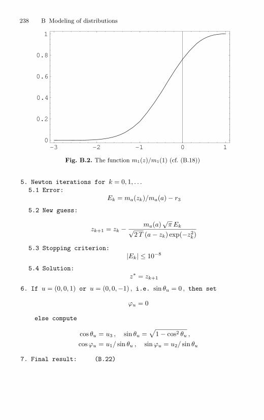
238 B Modeling of distributions
-3 -2 -1 0 10
0.2
0.4
0.6
0.8
1
Fig. B.2. The function m1(z)/m1(1) (cf. (B.18))
5. Newton iterations for k = 0, 1, . . .5.1 Error:
Ek = ma(zk)/ma(a) − r3
5.2 New guess:
zk+1 = zk − ma(a)√
π Ek√2T (a − zk) exp(−z2
k)
5.3 Stopping criterion:|Ek| ≤ 10−8
5.4 Solution:z∗ = zk+1
6. If u = (0, 0, 1) or u = (0, 0,−1) , i.e. sin θu = 0 , then set
ϕu = 0
else compute
cos θu = u3 , sin θu =√
1 − cos2 θu ,
cos ϕu = u1/ sin θu , sin ϕu = u2/ sin θu
7. Final result: (B.22)

B.6 Initial distribution of the BKW solution 239
B.6 Initial distribution of the BKW solution
Here we generate a random variable ξ according to the probability density (cf.(A.35))
pξ(v) =(
β + 12π T
)3/2 [1 + β
(β + 12T
|v|2 − 32
)]exp(− β + 1
2T|v|2), v ∈ R
3 ,
where β ∈ [0, 2/3] and T > 0 are some parameters. We apply the transforma-tion method (cf. Section B.1.2).
Using the substitution
v =(
β + 1T
)−1/2
w , dv =(
β + 1T
)−3/2
dw (B.23)
and switching to spherical coordinates
w = r e , 0 ≤ r < ∞ , e ∈ S2 , dw = r2 dr de (B.24)
one obtains
pη(r, e) =1
(2π)3/2r2
(1 + β
(12
r2 − 32
))exp(−r2/2) .
The components r and e of the random variable η are independent. Since thevector e is uniformly distributed on the unit sphere, we define
e∗ = UniSphere(r1, r2)
and it remains to solve the equation
F (r∗) :=
r∗∫0
r2
(1 + β
(12r2 − 3
2
))exp(− r2/2
)dr =
√π
2r3 , (B.25)
where r1, r2 and r3 denote random numbers uniformly distributed on (0, 1) .According to (B.23), (B.24), one obtains
ξ =(
β + 1T
)−1/2
r∗ e∗ . (B.26)
The nonlinear equation (B.25) is solved using the Newton method. Inte-grating by parts we express the function F in the form (see Fig. B.3)
F (z) = −(
z +β
2z3
)exp(− z2/2
)+√
π
2erf( z√
2
). (B.27)
The first two derivatives are
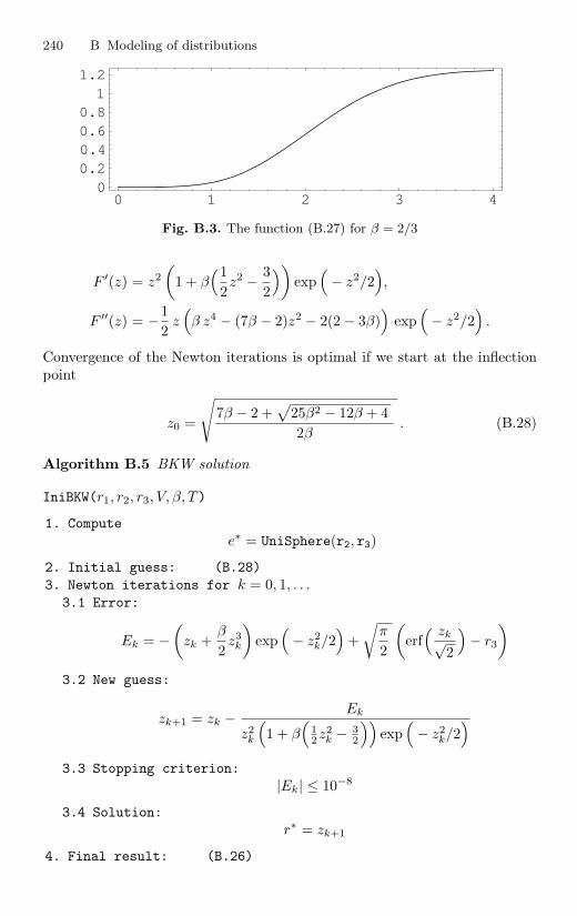
240 B Modeling of distributions
0 1 2 3 40
0.20.40.60.8
11.2
Fig. B.3. The function (B.27) for β = 2/3
F ′(z) = z2
(1 + β
(12z2 − 3
2
))exp(− z2/2
),
F ′′(z) = −12
z(β z4 − (7β − 2)z2 − 2(2 − 3β)
)exp(− z2/2
).
Convergence of the Newton iterations is optimal if we start at the inflectionpoint
z0 =
√7β − 2 +
√25β2 − 12β + 42β
. (B.28)
Algorithm B.5 BKW solution
IniBKW(r1, r2, r3, V, β, T)
1. Computee∗ = UniSphere(r2, r3)
2. Initial guess: (B.28)3. Newton iterations for k = 0, 1, . . .
3.1 Error:
Ek = −(
zk +β
2z3
k
)exp(− z2
k/2)
+√
π
2
(erf( zk√
2
)− r3
)
3.2 New guess:
zk+1 = zk − Ek
z2k
(1 + β
(12z2
k − 32
))exp(− z2
k/2)
3.3 Stopping criterion:|Ek| ≤ 10−8
3.4 Solution:r∗ = zk+1
4. Final result: (B.26)
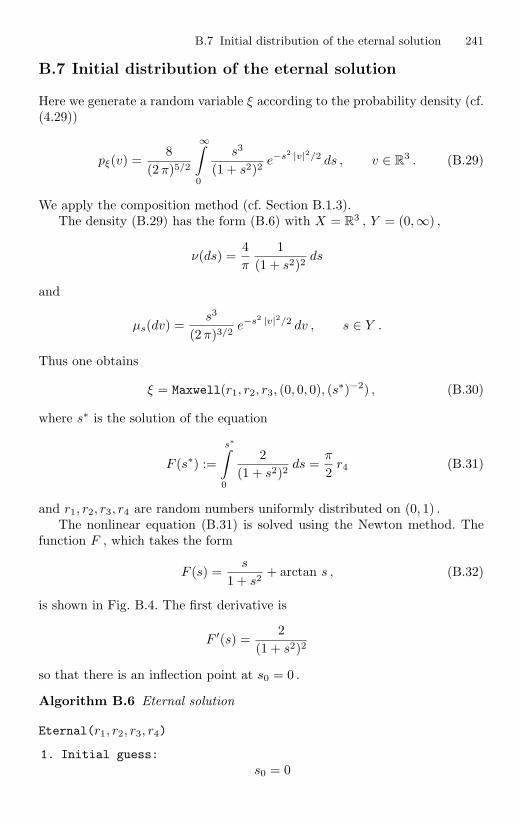
B.7 Initial distribution of the eternal solution 241
B.7 Initial distribution of the eternal solution
Here we generate a random variable ξ according to the probability density (cf.(4.29))
pξ(v) =8
(2π)5/2
∞∫0
s3
(1 + s2)2e−s2 |v|2/2 ds , v ∈ R
3 . (B.29)
We apply the composition method (cf. Section B.1.3).The density (B.29) has the form (B.6) with X = R
3 , Y = (0,∞) ,
ν(ds) =4π
1(1 + s2)2
ds
and
µs(dv) =s3
(2π)3/2e−s2 |v|2/2 dv , s ∈ Y .
Thus one obtains
ξ = Maxwell(r1, r2, r3, (0, 0, 0), (s∗)−2) , (B.30)
where s∗ is the solution of the equation
F (s∗) :=
s∗∫0
2(1 + s2)2
ds =π
2r4 (B.31)
and r1, r2, r3, r4 are random numbers uniformly distributed on (0, 1) .The nonlinear equation (B.31) is solved using the Newton method. The
function F , which takes the form
F (s) =s
1 + s2+ arctan s , (B.32)
is shown in Fig. B.4. The first derivative is
F ′(s) =2
(1 + s2)2
so that there is an inflection point at s0 = 0 .
Algorithm B.6 Eternal solution
Eternal(r1, r2, r3, r4)
1. Initial guess:s0 = 0

242 B Modeling of distributions
0 1 2 3 40
0.25
0.5
0.75
1
1.25
1.5
Fig. B.4. The function (B.32)
2. Newton iterations for k = 0, 1, . . .2.1 Error:
Ek =sk
1 + s2k
+ arctan sk − π
2r4
2.2 New guess:
sk+1 = sk − (1 + s2k)2
2Ek
2.3 Stopping criteria:|Ek| ≤ 10−8
2.4 Solution:s∗ = sk+1
3. Final result: (B.30)

References
1. F. J. Alexander, A. L. Garcia, and B. J. Alder. A consistent Boltzmann algo-rithm. Phys. Rev. Lett., 74(26):5212–5215, 1995.
2. F. J. Alexander, A. L. Garcia, and B. J. Alder. Cell size dependence of transportcoefficients in stochastic particle algorithms. Phys. Fluids, 10(6):1540–1542,1998.
3. H. L. Anderson. Scientific uses of the MANIAC. J. Statist. Phys., 43(5-6):731–748, 1986.
4. L. Arkeryd. On the Boltzmann equation. Part I. Existence. Arch. RationalMech. Anal., 45:1–16, 1972.
5. A. A. Arsenev. Approximation of the solution of the Boltzmann equation bysolutions of Ito stochastic differential equations. Zh. Vychisl. Mat. i Mat. Fiz.,27(3):400–410, 1987. In Russian.
6. A. A. Arsenev. Approximation of the Boltzmann equation by stochastic equa-tions. Zh. Vychisl. Mat. i Mat. Fiz., 28(4):560–567, 1988. In Russian.
7. H. Babovsky. On a simulation scheme for the Boltzmann equation. Math.Methods Appl. Sci., 8:223–233, 1986.
8. H. Babovsky. A convergence proof for Nanbu’s Boltzmann simulation scheme.European J. Mech. B Fluids, 8(1):41–55, 1989.
9. H. Babovsky. Time averages of simulation schemes as approximations to sta-tionary kinetic equations. European J. Mech. B Fluids, 11(2):199–212, 1992.
10. H. Babovsky. Monte Carlo simulation schemes for steady kinetic equations.Transport Theory Statist. Phys., 23(1-3):249–264, 1994.
11. H. Babovsky. Die Boltzmann-Gleichung: Modellbildung–Numerik–Anwendun-gen. B. G. Teubner, Stuttgart, 1998.
12. H. Babovsky and R. Illner. A convergence proof for Nanbu’s simulation methodfor the full Boltzmann equation. SIAM J. Numer. Anal., 26(1):45–65, 1989.
13. O. M. Belotserkovskij, A. I. Erofeev, and V. E. Yanitskij. A nonstationarymethod for direct statistical simulation of rarefied gas flows. Zh. Vychisl. Mat.i Mat. Fiz., 20(5):1174–1204, 1980. In Russian.
14. O. M. Belotserkovskij, A. I. Erofeev, and V. E. Yanitskij. Direct statisticalmodelling of problems in aero-gas dynamics. Adv. in Mech., 5(3/4):11–40,1982. In Russian.
15. O. M. Belotserkovskij and V. E. Yanitskij. Statistical particle in cell methodfor problems in rarefied gas dynamics. I. Construction of the method. Zh.Vychisl. Mat. i Mat. Fiz., 15(5):1195–1209, 1975. In Russian.

244 References
16. O. M. Belotserkovskij and V. E. Yanitskij. Statistical particle in cell methodfor problems in rarefied gas dynamics. II. Numerical aspects of the method.Zh. Vychisl. Mat. i Mat. Fiz., 15:1553–1567, 1975. In Russian.
17. P. H. Bezandry, R. Ferland, G. Giroux, and J.-C. Roberge. Une approche prob-abiliste de resolution d’equations non lineaires. In Measure-valued processes,stochastic partial differential equations, and interacting systems (Montreal, PQ,1992), volume 5 of CRM Proc. Lecture Notes, pages 17–33. Amer. Math. Soc.,Providence, RI, 1994.
18. P. H. Bezandry, X. Fernique, and G. Giroux. A functional central limit theoremfor a nonequilibrium model of interacting particles with unbounded intensity.J. Statist. Phys., 72(1/2):329–353, 1993.
19. G. A. Bird. Approach to translational equilibrium in a rigid sphere gas. Phys.Fluids, 6:1518–1519, 1963.
20. G. A. Bird. Shock wave structure in a rigid sphere gas. In J.H. de Leeuw,editor, Rarefied Gas Dynamics, volume 1, pages 216–222. Academic Press, NewYork, 1965.
21. G. A. Bird. Molecular Gas Dynamics. Clarendon Press, Oxford, 1976.22. G. A. Bird. Transition regime behavior of supersonic beam skimmers. Phys.
Fluids, 19(10):1486–1491, 1976.23. G. A. Bird. Monte–Carlo simulation in an engineering context. In S. Fisher,
editor, Proc. of the 12th International Symposium on Rarefied Gas Dynamics(Charlottesville, 1980), volume 74 of Progress in Astronautics and Aeronautics,pages 239–255. AIAA, New York, 1981.
24. G. A. Bird. Perception of numerical methods in rarefied gas dynamics. Progr.Astronaut. Aeronaut., 118:211–226, 1989.
25. G. A. Bird. Molecular Gas Dynamics and the Direct Simulation of Gas Flows.Clarendon Press, Oxford, 1994.
26. G. A. Bird. Forty years of DSMC, and now? In T. J. Bartel and M. A. Gal-lis, editors, Rarefied Gas Dynamics, 22nd International Symposium, Sydney,Australia, 9-14 July 2000, volume 585 of AIP Conference Proceedings, pages372–380. AIP Publishing Center, New York, 2001.
27. A. V. Bobylev. Exact solutions of the Boltzmann equation. Dokl. Akad. NaukSSSR, 225(6):1296–1299, 1975. In Russian.
28. A. V. Bobylev and C. Cercignani. Exact eternal solutions of the Boltzmannequation. J. Statist. Phys., 106(5-6):1019–1038, 2002.
29. A. V. Bobylev and C. Cercignani. The inverse Laplace transform of someanalytic functions with an application to the eternal solutions of the Boltzmannequation. Appl. Math. Lett., 15(7):807–813, 2002.
30. A. V. Bobylev and C. Cercignani. Moment equations for a granular materialin a thermal bath. J. Statist. Phys., 106(3-4):547–567, 2002.
31. A. V. Bobylev and T. Ohwada. On the generalization of Strang’s splittingscheme. Riv. Mat. Univ. Parma (6), 2*:235–243, 1999.
32. A. V. Bobylev and T. Ohwada. The error of the splitting scheme for solvingevolutionary equations. Appl. Math. Lett., 14(1):45–48, 2001.
33. A. V. Bobylev and S. Rjasanow. Numerical solution of the Boltzmann equationusing a fully conservative difference scheme based on the fast Fourier transform.Transport Theory Statist. Phys., 29(3-5):289–310, 2000.
34. A. V. Bobylev and J. Struckmeier. Numerical simulation of the stationaryone-dimensional Boltzmann equation by particle methods. European J. Mech.B Fluids, 15(1):103–118, 1996.

References 245
35. S. V. Bogomolov. Convergence of the method of summary approximation forthe Boltzmann equation. Zh. Vychisl. Mat. i Mat. Fiz., 28(1):119–126, 1988.In Russian.
36. L. Boltzmann. Weitere Studien uber das Warmegleichgewicht unter Gas-molekulen. Sitzungsber. Akad. Wiss. Wien, 66:275–370, 1872.
37. J.-F. Bourgat, P. Le Tallec, B. Perthame, and Y. Qiu. Coupling Boltzmannand Euler equations without overlapping. In Domain decomposition methodsin science and engineering (Como, 1992), pages 377–398. Amer. Math. Soc.,Providence, RI, 1994.
38. I. Boyd, G. Chen, and G. Candler. Predicting Failure of the Continuum FluidEquations. AIAA, 94:2352, 1994.
39. I. D. Boyd. Conservative species weighting scheme for the direct simulationMonte Carlo method. J. of Thermophysics and Heat Transfer, 10(4):579–585,1996.
40. G. Brasseur and S. Solomon. Aeronomy of the Middle Atmosphere. D. ReidelPublishing Company, Dordrecht, 1984.
41. N. P. Buslenko, D. I. Golenko, Yu. A. Shreider, I. M. Sobol, and V. G.Sragovich. The Monte Carlo method. The method of statistical trials. In-ternational Series of Monographs in Pure and Applied Mathematics, Vol. 87.Pergamon Press, Oxford, 1966.
42. N. P. Buslenko, D. I. Golenko, I. M. Sobol, V. G. Sragovich, and Ju. A. Shreider.Metod statisticheskikh ispytanii (Metod Monte-Karlo). Gosudarstv. Izdat. Fiz.-Mat. Lit., Moscow, 1962. (Russian) [The method of statistical testing (TheMonte Carlo method)] English translation: [41].
43. N. P. Buslenko and Ju. A. Shreider. Metod statisticheskikh ispytanii (Monte-Karlo) i ego realizatsiya na tsifrovykh vychislitelnykh mashinakh. BibliotekaPrikladnogo Analiza i Vycislitelnoı Matematiki. Gosudarstv. Izdat. Fiz-Mat.Lit., Moscow, 1961. (Russian) [The Monte-Carlo method and how it is carriedout on digital computers].
44. S. Caprino and M. Pulvirenti. A cluster expansion approach to a one–dimensional Boltzmann equation: a validity result. Comm. Math. Phys.,166:603–631, 1995.
45. S. Caprino, M. Pulvirenti, and W. Wagner. Stationary particle systems ap-proximating stationary solutions to the Boltzmann equation. SIAM J. Math.Anal., 29(4):913–934, 1998.
46. C. Cercignani. On the master equation in the space inhomogeneous case.In Theories cinetiques classiques et relativistes, Colloques InternationauxC.N.R.S. 236 (Paris 1974), pages 209–221, 1975.
47. C. Cercignani. The Grad limit for a system of soft spheres. Comm. Pure Appl.Math., 36(4):479–494, 1983.
48. C. Cercignani. The Boltzmann Equation and its Applications. Springer, NewYork, 1988.
49. C. Cercignani. Ludwig Boltzmann. The Man who Trusted Atoms. OxfordUniversity Press, Oxford, 1998.
50. C. Cercignani. Rarefied Gas Dynamics. From Basic Concepts to Actual Cal-culations. Cambridge Texts in Applied Mathematics. Cambridge UniversityPress, 2000.
51. C. Cercignani, R. Illner, and M. Pulvirenti. The Mathematical Theory of DiluteGases. Springer, New York, 1994.
246 References
52. E. G. D. Cohen, W. Fiszdon, and A. Palczewski, editors. Fundamental problemsin statistical mechanics. IV. Ossolineum, Wroc�law, 1978. Proceedings of theFourth International Summer School in Statistical Mechanics, held in Jadwisin,September 14–24, 1977.
53. M. H. A. Davis. Piecewise–deterministic Markov processes: A general class ofnon–diffusion stochastic models. J. Roy. Statist. Soc. Ser. B, 46(3):353–388,1984.
54. M. H. A. Davis. Markov Models and Optimization. Chapman & Hall, London,1993.
55. S. M. Deshpande. The statistical particle–in–cell method for multicomponentgases. Zh. Vychisl. Mat. i Mat. Fiz., 23(1):170–177, 1983.
56. S. M. Ermakov. Metod Monte-Karlo i smezhnye voprosy. Nauka, Moscow,1971. (Russian) [The Monte Carlo method and related problems].
57. S. M. Ermakov and N. M. Moskaleva. Branching processes and the Boltzmannequation. Numerical aspects. Vestnik Leningrad Univ. Ser. 1, 3:38–43, 1987.In Russian.
58. S. M. Ermakov, V. V. Nekrutkin, and A. S. Sipin. Sluchainye protsessy dlyaresheniya klassicheskikh uravnenii matematicheskoi fiziki. Nauka, Moscow,1984. English translation: [59].
59. S. M. Ermakov, V. V. Nekrutkin, and A. S. Sipin. Random Processes forClassical Equations of Mathematical Physics, volume 34 of Mathematics and itsApplications (Soviet Series). Kluwer Academic Publishers Group, Dordrecht,1989.
60. M. H. Ernst. Exact solutions of the nonlinear Boltzmann and related kineticequations. In Nonequilibrium phenomena. I. The Boltzmann equation, pages51–119. North–Holland, 1983.
61. S. N. Ethier and T. G. Kurtz. Markov Processes, Characterization and Con-vergence. Wiley, New York, 1986.
62. J. Fan and C. Shen. Statistical simulation of low-speed rarefied gas flows. J.Comput. Phys., 167:393–412, 2001.
63. W. Feller. Zur Theorie der stochastischen Prozesse. Math. Ann., 113:113–160,1937.
64. R. Ferland, X. Fernique, and G. Giroux. Compactness of the fluctuationsassociated with some generalized nonlinear Boltzmann equations. Can. J.Math., 44(6):1192–1205, 1992.
65. A. Frezzotti. A particle scheme for the numerical solution of the Enskog equa-tion. Phys. Fluids, 9(5):1329–1335, 1997.
66. T. Funaki. Construction of stochastic processes associated with the Boltz-mann equation and its applications. In K. Ito and T. Hida, editors, Stochasticprocesses and their applications, volume 1203 of Lecture Notes in Mathematics,pages 51–65. Springer, Berlin/Heidelberg, 1986.
67. A. L. Garcia and W. Wagner. The limiting kinetic equation of the consistentBoltzmann algorithm for dense gases. J. Statist. Phys., 101(5-6):1065–1086,2000.
68. A. L. Garcia and W. Wagner. Time step truncation error in direct simulationMonte Carlo. Phys. Fluids, 12(10):2621–2633, 2000.
69. A. L. Garcia and W. Wagner. Some new properties of the kinetic equationfor the Consistent Boltzmann Algorithm. Transport Theory Statist. Phys.,31(4-6):579–594, 2002.

References 247
70. A. L. Garcia and W. Wagner. Direct simulation Monte Carlo method for theUehling-Uhlenbeck-Boltzmann equation. Physical Review E, 68(056703):1–11,2003.
71. D. I. Golenko. Modelirovanie i statisticheskii analiz psevdosluchainykh chiselna elektronnykh vychislitelnykh mashinakh. Izdat. “Nauka”, Moscow, 1965.(Russian) [Simulation and statistical analysis of pseudo-random numbers onelectronic computing machines].
72. C. Graham and S. Meleard. Stochastic particle approximations for generalizedBoltzmann models and convergence estimates. Ann. Probab., 25(1):115–132,1997.
73. F. A. Grunbaum. Propagation of chaos for the Boltzmann equation. Arch.Rational Mech. Anal., 42(5):323–345, 1971.
74. M. Gunther, P. Le Tallec, J. P. Perlat, and J. Struckmeier. Numerical model-ing of gas flows in the transition between rarefied and continuum regimes. InNumerical flow simulation, I (Marseille, 1997), pages 222–241. Vieweg, Braun-schweig, 1998.
75. N. G. Hadjiconstantinou. Analysis of discretization in direct simulation MonteCarlo. Phys. Fluids, 12(10):2634–2638, 2000.
76. J. H. Halton. A retrospective and prospective survey of the Monte Carlomethod. SIAM Rev., 12:1–63, 1970.
77. J. M. Hammersley and D. C. Handscomb. Monte Carlo methods. Methuen &Co. Ltd., London, 1965.
78. H. A. Hassan and D. B. Hash. A generalized hard-sphere model for MonteCarlo simulations. Phys. Fluids A, 5 : 738–744, 1993.
79. J. K. Haviland and M. L. Lavin. Application of the Monte Carlo method toheat transfer in a rarefied gas. Phys. Fluids, 5(11):1399–1405, 1962.
80. T. Hokazono, S. Kobayashi, T. Ohsawa, and T. Ohwada. On the time steperror of the DSMC. In A. D. Ketsdever and E. P. Muntz, editors, Rarefied GasDynamics, pages 390–397. AIP Publishing Center, New York, 2003.
81. J. Horowitz and R. L. Karandikar. Martingale problems associated with theBoltzmann equation. In Seminar on Stochastic Processes, 1989, volume 18 ofProgress in Probability, pages 75–122. Birkhauser, Boston/Basel/Berlin, 1990.
82. K. Huang. Statistical mechanics. John Wiley & Sons Inc., New York, secondedition, 1987.
83. R. Illner and H. Neunzert. On simulation methods for the Boltzmann equation.Transport Theory Statist. Phys., 16(2&3):141–154, 1987.
84. R. Illner and S. Rjasanow. Random discrete velocity models: Possible bridgesbetween the Boltzmann equation, discrete velocity models and particle simu-lation? In V. C. Boffi, F. Bampi, and G. Toscani, editors, Nonlinear kinetictheory and mathematical aspects of hyperbolic systems, pages 152–158. WorldScientific, Singapore, 1992.
85. R. Illner and S. Rjasanow. Numerical solution of the Boltzmann equation byrandom discrete velocity models. European J. Mech. B Fluids, 13(2):197–210,1994.
86. R. Illner and W. Wagner. A random discrete velocity model and approximationof the Boltzmann equation. J. Statist. Phys., 70(3/4):773–792, 1993.
87. R. Illner and W. Wagner. Random discrete velocity models and approximationof the Boltzmann equation. Conservation of momentum and energy. TransportTheory Statist. Phys., 23(1–3):27–38, 1994.

248 References
88. M. S. Ivanov and S. V. Rogasinsky. Theoretical analysis of traditional andmodern schemes of the DSMC method. In A. E. Beylich, editor, Proc. ofthe 17th International Symposium on Rarefied Gas Dynamics, pages 629–642,Aachen, 1990.
89. M. S. Ivanov and S. V. Rogazinskij. Comparative analysis of algorithms of thedirect statistical modeling method in rarefied gas dynamics. Zh. Vychisl. Mat.i Mat. Fiz., 28(7):1058–1070, 1988. In Russian.
90. M. S. Ivanov and S. V. Rogazinskij. Efficient schemes for direct statisticalmodeling of rarefied gas flows. Mat. Model., 1(7):130–145, 1989. In Russian.
91. M. Kac. Foundations of kinetic theory. In Third Berkeley Symposium onMathematical Statistics and Probability Theory, volume 3, pages 171–197, 1956.
92. M. Kac. Some Stochastic Problems in Physics and Mathematics. MagnoliaPetroleum Co., 1956.
93. M. Kac. Probability and Related Topics in Physical Sciences. Interscience,London, 1959.
94. M. Kac. Veroyatnost’ i smezhnye voprosy v fizike. Mir, Moscow, 1965. Russiantranslation of [93].
95. M. Kac. Neskol’ko veroyatnostnykh zadach fiziki i matematiki. Nauka, Moscow,1967. Russian translation of the Polish edition of [92].
96. M. Kac. Some probabilistic aspects of the Boltzmann equation. Acta Phys.Austriaca, Suppl. X:379–400, 1973.
97. M. Kac. Nonlinear dynamics and inverse problems. In Fundamental problemsin statistical mechanics, IV (Proc. Fourth Internat. Summer School, Jadwisin,1977), pages 199–222. Ossolineum, Wroc�law, 1978.
98. M. Kac and J. Logan. Fluctuations. In Fluctuation Phenomena, volume VIIof Studies in Statistical Mechanics, pages 1–60. North-Holland, 1979.
99. A. I. Khisamutdinov. A simulation method for statistical modeling of rarefiedgases. Dokl. Akad. Nauk SSSR, 291(6):1300–1304, 1986. In Russian.
100. R. Kirsch. Die Boltzmann-Gleichung fur energieabhangige Verteilungsfunktio-nen. Diplomarbeit, Universitat des Saarlandes, 1999.
101. A. Klar. Convergence of alternating domain decomposition schemes for kineticand aerodynamic equations. Math. Methods Appl. Sci., 18(8):649–670, 1995.
102. A. Klar. Domain decomposition for kinetic problems with nonequilibriumstates. European J. Mech. B Fluids, 15(2):203–216, 1996.
103. A. Klar. Asymptotic analysis and coupling conditions for kinetic and hydro-dynamic equations. Comput. Math. Appl., 35(1-2):127–137, 1998.
104. Yu. L. Klimontovich. Kinetic theory of fluctuations in gases and plasma.In Fundamental problems in statistical mechanics, IV (Proc. Fourth Internat.Summer School, Jadwisin, 1977), pages 265–309. Ossolineum, Wroc�law, 1978.
105. Yu. L. Klimontovich. Dissipative equations for many-particle distribution func-tions. Uspekhi Fiz. Nauk, 139(4):689–700, 1983. In Russian.
106. Yu. L. Klimontovich. Statistical theory of open systems. Vol. 1, volume 67 ofFundamental Theories of Physics. Kluwer Academic Publishers Group, Dor-drecht, 1995.
107. M. Knudsen. Kinetic Theory of Gases. Methuen, London, 1952.108. A. Kolmogoroff. Uber die analytischen Methoden in der Wahrscheinlichkeit-
srechnung. Math. Ann., 104:415–458, 1931.109. A. Kolmogoroff and M. Leontowitsch. Zur Berechnung der mittleren Brown-
schen Flache. Physik. Zeitschr. d. Sowjetunion, 4:1–13, 1933.

References 249
110. A. N. Kolmogoroff. Grundbegriffe der Wahrscheinlichkeitsrechnung. Springer,Berlin, 1933.
111. Yu. N. Kondyurin. A statistical approach to the solution of the Boltzmannequation. Zh. Vychisl. Mat. i Mat. Fiz., 26(10):1527–1534, 1986. In Russian.
112. K. Koura. Null–collision technique in the direct–simulation Monte Carlomethod. Phys. Fluids, 29(11):3509–3511, 1986.
113. K. Koura and H. Matsumoto. Variable soft sphere molecular model for inverse-power-law or Lennard-Jones potential. Phys. Fluids A, 3 : 2459–2465, 1991.
114. K. Koura and H. Matsumoto. Variable soft sphere molecular model for airspecies. Phys. Fluids A, 4 : 1083–1085, 1992.
115. M. Krook and T. T. Wu. Exact solutions of the Boltzmann equation. Phys.Fluids, 20(10):1589–1595, 1977.
116. M. Lachowicz and M. Pulvirenti. A stochastic system of particles modellingthe Euler equation. Arch. Rational Mech. Anal., 109(1):81–93, 1990.
117. P. Le Tallec and F. Mallinger. Coupling Boltzmann and Navier-Stokes equa-tions by half fluxes. J. Comput. Phys., 136(1):51–67, 1997.
118. C. Lecot. A direct simulation Monte Carlo scheme and uniformly distributed se-quences for solving the Boltzmann equation. Computing, 41(1/2):41–57, 1989.
119. C. Lecot. Low discrepancy sequences for solving the Boltzmann equation. J.Comput. Appl. Math., 25(2):237–249, 1989.
120. C. Lecot. A quasi-Monte Carlo method for the Boltzmann equation. Math.Comp., 56(194):621–644, 1991.
121. M. A. Leontovich. Basic equations of the kinetic gas theory from the pointof view of the theory of random processes. Zhurnal Teoret. Ehksper. Fiziki,5(3-4):211–231, 1935. In Russian.
122. M. Leontowitsch. Zur Statistik der kontinuierlichen Systeme und des zeitlichenVerlaufes der physikalischen Vorgange. Physik. Zeitschr. d. Sowjetunion, 3:35–63, 1933.
123. H. W. Liepmann, R. Narasimha, and M. T. Chahine. Structure of a planeshock layer. Phys. Fluids, 5:1313, 1962.
124. J. Logan and M. Kac. Fluctuations and the Boltzmann equation. Phys. Rev.A, 13(1):458–470, 1976.
125. A. V. Lukshin. A stochastic method for solving the Boltzmann equationfor a gas with an arbitrary interaction law. Differentsial’nye Uravneniya,23(11):2001–2004, 1987. In Russian.
126. A. V. Lukshin. Stochastic algorithms of the mathematical theory of the spa-tially inhomogeneous Boltzmann equation. Mat. Model., 1(7):146–159, 1989.In Russian.
127. A. V. Lukshin and S. N. Smirnov. On a stochastic method for solving theBoltzmann equation. Zh. Vychisl. Mat. i Mat. Fiz., 28(2):293–297, 1988. InRussian.
128. A. V. Lukshin and S. N. Smirnov. An efficient stochastic algorithm for solvingthe Boltzmann equation. Zh. Vychisl. Mat. i Mat. Fiz., 29(1):118–124, 1989.In Russian.
129. A. V. Lukshin and I. E. Yuferov. Stochastic algorithms for solving the spatiallyhomogeneous Boltzmann equation for gas mixtures. Mat. Model., 1(2):151–160,1989. In Russian.
130. I. Matheis and W. Wagner. Convergence of the stochastic weighted particlemethod for the Boltzmann equation. SIAM J. Sci. Comput., 24(5):1589–1609,2003.

250 References
131. M. J. McEwan and L. F. Phillips. The Chemistry of the Atmosphere. EdwardArnold (Publishers) Ltd., London, 1975.
132. H. P. McKean. Speed of approach to equilibrium for Kac’s caricature of aMaxwellian gas. Arch. Rational Mech. Anal., 21:343–367, 1966.
133. H. P. McKean. An exponential formula for solving Boltzmann’s equation fora Maxwellian gas. J. Combin. Theory, 2:358–382, 1967.
134. H. P. McKean. Fluctuations in the kinetic theory of gases. Comm. Pure Appl.Math., 28(4):435–455, 1975.
135. J. Meixner. Zur Thermodynamik irreversibler Prozesse. Z. Phys. Chem., 53B:253, 1941.
136. S. Meleard. Stochastic approximations of the solution of a full Boltzmannequation with small initial data. ESAIM Probab. Statist., 2:23–40 (electronic),1998.
137. N. Metropolis and S. Ulam. The Monte Carlo method. J. Amer. Statist. Assoc.,44:335–341, 1949.
138. G. A. Mikhailov and S. V. Rogazinskii. Weighted Monte Carlo methods forthe approximate solution of the nonlinear Boltzmann equation. Sibirsk. Mat.Zh., 43(3):620–628, 2002. In Russian.
139. J. M. Montanero and A. Santos. Simulation of the Enskog equation a la Bird.Phys. Fluids, 9:2057–2060, 1997.
140. D. Morgenstern. Analytical studies related to the Maxwell–Boltzmann equa-tion. J. Rational Mech. Anal., 4:533–555, 1955.
141. H. Mott-Smith. The solution of the Boltzmann equation for a shock wave.Phys. Rev., 82:885–892, 1951.
142. C. Muckenfuss. Some aspects of shock structure according to the bimodalmodel. Phys. Fluids, 5(11):1325–1336, 1962.
143. H. Murata. Propagation of chaos for Boltzmann-like equations of noncutoff–type in the plane. Hiroshima Math. J., 7:479–515, 1977.
144. K. Nanbu. Direct simulation scheme derived from the Boltzmann equation. I.Monocomponent gases. J. Phys. Soc. Japan, 49(5):2042–2049, 1980.
145. K. Nanbu. Interrelations between various direct simulation methods for solvingthe Boltzmann equation. J. Phys. Soc. Japan, 52(10):3382–3388, 1983.
146. K. Nanbu. Theoretical basis of the direct simulation Monte Carlo method. InV. Boffi and C. Cercignani, editors, Rarefied Gas Dynamics, volume 1, pages369–383. Teubner, Stuttgart, 1986.
147. K. Nanbu. Weighted particles in Coulomb collision simulations based on thetheory of a cumulative scattering angle. J. Comput. Phys., 145:639–654, 1998.
148. V. Nekrutkin and N. Tur. Asymptotic expansions and estimators with smallbias for Nanbu processes. Monte Carlo Methods Appl., 3(1):1–35, 1997.
149. V. V. Nekrutkin and N. I. Tur. On the justification of a scheme of directmodelling of flows of rarefied gases. Zh. Vychisl. Mat. i Mat. Fiz., 29(9):1380–1392, 1989. In Russian.
150. H. Neunzert, F. Gropengiesser, and J. Struckmeier. Computational methodsfor the Boltzmann equation. In Applied and industrial mathematics (Venice,1989), volume 56 of Math. Appl., pages 111–140. Kluwer Acad. Publ., Dor-drecht, 1991.
151. H. Neunzert, A. Klar, and J. Struckmeier. Particle methods: theory and ap-plications. In ICIAM 95 (Hamburg, 1995), pages 281–306. Akademie Verlag,Berlin, 1996.

References 251
152. H. Neunzert and J. Struckmeier. The finite pointset method for hypersonicflows in the rarefied gas regime. In Advances in hypersonics, Vol. 3 (ColoradoSprings, CO, 1989; Aachen, 1990), pages 342–370. Birkhauser Boston, Boston,MA, 1992.
153. H. Neunzert and J. Struckmeier. Particle methods for the Boltzmann equa-tion. In Acta Numerica 1995, pages 417–457. Cambridge University Press,Cambridge, 1995.
154. A. Nordsieck, W. E. Lamb, Jr., and G. E. Uhlenbeck. On the theory of cosmic–ray showers. I. The furry model and the fluctuation problem. Physica, 7(4):344–360, 1940.
155. T. Ohwada. Higher order approximation methods for the Boltzmann equation.J. Comput. Phys., 139:1–14, 1998.
156. T. Ohwada. Higher order time integration of spatially nonhomogeneous Boltz-mann equation: deterministic and stochastic computations. Transport TheoryStatist. Phys., 29(3-5):495–508, 2000.
157. G. C. Papanicolaou. Asymptotic analysis of transport processes. Bull. Amer.Math. Soc., 81(2):330–392, 1975.
158. L. Pareschi and R. E. Caflisch. An implicit Monte Carlo method for rarefied gasdynamics. I. The space homogeneous case. J. Comput. Phys., 154(1):90–116,1999.
159. L. Pareschi and G. Russo. Time relaxed Monte Carlo methods for the Boltz-mann equation. SIAM J. Sci. Comput., 23(4):1253–1273, 2001.
160. L. Pareschi and B. Wennberg. A recursive Monte Carlo method for the Boltz-mann equation in the Maxwellian case. Monte Carlo Methods Appl., 7(3-4):349–357, 2001.
161. G. Pichon. Sur la propagation du chaos moleculaire. C. R. Acad. Sci. ParisSer. A, 274:1667–1670, 1972.
162. G. Pichon. Chaos moleculaire et equation de Boltzmann. C. R. Acad. Sci.Paris Ser. A, 276:583–585, 1973.
163. G. Pichon. Chaos moleculaire et equation de Boltzmann. J. Math. Pures Appl.,53(2):183–195, 1974.
164. G. Pichon. Chaos moleculaire et equation de Boltzmann. In Theories cinetiquesclassiques et relativistes, Colloques Internationaux C.N.R.S. 236 (Paris 1974),pages 195–207, 1975.
165. H. Ploss. On simulation methods for solving the Boltzmann equation. Com-puting, 38:101–115, 1987.
166. A. Ya. Povzner. On the Boltzmann equation in kinetic gas theory. Matem.Sb., 58(1):65–86, 1962. In Russian.
167. M. Pulvirenti, W. Wagner, and M. B. Zavelani Rossi. Convergence of particleschemes for the Boltzmann equation. European J. Mech. B Fluids, 13(3):339–351, 1994.
168. P. Quell. Nonlinear stability of entropy flux splitting schemes on boundeddomains. IMA J. Numer. Anal., 20(3):441–459, 2000.
169. A. K. Rebrov and P. A. Skovorodko. An improved sampling procedure inDSMC method. In C. Shen, editor, Rarefied Gas Dynamics, pages 215–220.Peking University Press, Beijing, 1997.
170. F. Rezakhanlou. Kinetic limits for a class of interacting particle systems.Probab. Theory Related Fields, 104(1):97–146, 1996.
171. F. Rezakhanlou. Propagation of chaos for particle systems associated withdiscrete Boltzmann equation. Stochastic Process. Appl., 64(1):55–72, 1996.

252 References
172. F. Rezakhanlou. A stochastic model associated with Enskog equation and itskinetic limit. Comm. Math. Phys., 232(2):327–375, 2003.
173. F. Rezakhanlou and J. E. Tarver. Boltzmann-Grad limit for a particle systemin continuum. Ann. Inst. H. Poincare Probab. Statist., 33(6):753–796, 1997.
174. Rarefied Gas Dynamics, Proceedings of the 23rd International Symposium(Whistler, Canada, 20-25 July 2002), eds. Ketsdever, A. D. and Muntz, E. P.,volume 663 of AIP Conference Proceedings, AIP Publishing Center, New York,2003.
175. Rarefied gas dynamics: Proceedings of the First International Symposium (Nice,France, 1958), International Series on Aeronautical Sciences and Space Flight,Division IX, Vol. 3, Pergamon Press, New York, 1960.
176. S. Rjasanow, T. Schreiber, and W. Wagner. Reduction of the number of par-ticles in the stochastic weighted particle method for the Boltzmann equation.J. Comput. Phys., 145(1):382–405, 1998.
177. S. Rjasanow and W. Wagner. A stochastic weighted particle method for theBoltzmann equation. J. Comput. Phys., 124(2):243–253, 1996.
178. S. Rjasanow and W. Wagner. A generalized collision mechanism for stochasticparticle schemes approximating Boltzmann-type equations. Comput. Math.Appl., 35(1/2):165–178, 1998.
179. S. Rjasanow and W. Wagner. On time counting procedures in the DSMCmethod for rarefied gases. Math. Comput. Simulation, 48(2):153–178, 1998.
180. S. Rjasanow and W. Wagner. A temperature time counter scheme for theBoltzmann equation. SIAM J. Numer. Anal., 37(6):1800–1819, 2000.
181. S. Rjasanow and W. Wagner. Simulation of rare events by the stochasticweighted particle method for the Boltzmann equation. Math. Comput. Mod-elling, 33(8-9):907–926, 2001.
182. S. V. Rogasinsky. Solution of stationary boundary value problems for theBoltzmann equation by the Monte Carlo method. Monte Carlo Methods Appl.,5(3):263–280, 1999.
183. M. Schreiner. Weighted particles in the finite pointset method. TransportTheory Statist. Phys., 22(6):793–817, 1993.
184. A. J. F. Siegert. On the approach to statistical equlibrium. Phys. Rev.,76(11):1708–1714, 1949.
185. A. V. Skorokhod. Stokhasticheskie uravneniya dlya slozhnykh sistem. Nauka,Moscow, 1983. English translation: [186].
186. A. V. Skorokhod. Stochastic Equations for Complex Systems, volume 13 ofMathematics and its Applications (Soviet Series). D. Reidel Publishing Co.,Dordrecht, 1988.
187. S. N. Smirnov. On the justification of a stochastic method for solving theBoltzmann equation. Zh. Vychisl. Mat. i Mat. Fiz., 29(2):270–276, 1989. InRussian.
188. I. M. Sobol. Chislennye metody Monte-Karlo. Izdat. “Nauka”, Moscow, 1973.(Russian) [Numerical Monte Carlo methods].
189. J. Spanier and E. M. Gelbard. Monte Carlo principles and neutron transportproblems. Addison-Wesley Publishing Co., Reading, Mass.-London-Don Mills,Ont., 1969.
190. J. Struckmeier and K. Steiner. A comparison of simulation methods for rarefiedgas flows. Phys. Fluids, 7(11):2876–2885, 1995.
191. Q. Sun and I.D. Boyd. A direct simulation method for subsonic, microscalegas flows. J. Comput. Phys., 179:400–425, 2002.

References 253
192. A.-S. Sznitman. Equations de type de Boltzmann, spatialement homogenes.C. R. Acad. Sci. Paris Ser. I Math., 295:363–366, 1982.
193. A. S. Sznitman. Equations de type de Boltzmann, spatialement homogenes.Z. Wahrsch. Verw. Gebiete, 66(4):559–592, 1984.
194. A. S. Sznitman. Topics in propagation of chaos. In Lecture Notes in Mathe-matics, volume 1464, pages 165–251. Springer, Berlin, 1991.
195. H. Tanaka. On Markov processes corresponding to the Boltzmann equation ofMaxwellian gas. In Lecture Notes in Mathematics, volume 330, pages 478–489.Springer, Berlin, 1973.
196. H. Tanaka. Probabilistic treatment of the Boltzmann equation of Maxwellianmolecules. Z. Wahrsch. Verw. Gebiete, 46(1):67–105, 1978.
197. H. Tanaka. Some probabilistic problems in the spatially homogeneous Boltz-mann equation. In G. Kallianpur, editor, Theory and Applications of RandomFields, volume 49 of Lecture Notes in Control and Inform. Sci., pages 258–267,Springer, Berlin, 1983.
198. C. J. Thompson. The contributions of Mark Kac to mathematical physics.Ann. Probab., 14(4):1129–1138, 1986.
199. S. Tiwari. Coupling of the Boltzmann and Euler equations with automaticdomain decomposition. J. Comput. Phys., 144(2):710–726, 1998.
200. S. Tiwari and A. Klar. An adaptive domain decomposition procedure forBoltzmann and Euler equations. J. Comput. Appl. Math., 90(2):223–237, 1998.
201. S. Tiwari and S. Rjasanow. Sobolev norm as a criterion of local thermalequilibrium. European J. Mech. B Fluids, 16(6):863–876, 1997.
202. H. F. Trotter and J. W. Tukey. Conditional Monte Carlo for normal samples.In Symposium on Monte Carlo methods, University of Florida, 1954, pages64–79. John Wiley and Sons, Inc., New York, 1956.
203. K. Uchiyama. Fluctuations in population dynamics. In M. Kimura, G. Kallian-pur, and T. Hida, editors, Stochastic Methods in Biology, volume 70 of LectureNotes in Biomathematics, pages 222–229, Springer, Berlin, 1987.
204. W. Wagner. A convergence proof for Bird’s direct simulation Monte Carlomethod for the Boltzmann equation. J. Statist. Phys., 66(3/4):1011–1044,1992.
205. W. Wagner. A stochastic particle system associated with the spatially inhomo-geneous Boltzmann equation. Transport Theory Statist. Phys., 23(4):455–477,1994.
206. W. Wagner. Stochastic systems of particles with weights and approximationof the Boltzmann equation. The Markov process in the spatially homogeneouscase. Stochastic Anal. Appl., 12(5):639–659, 1994.
207. W. Wagner. A functional law of large numbers for Boltzmann type stochasticparticle systems. Stochastic Anal. Appl., 14(5):591–636, 1996.
208. E. Wild. On Boltzmann’s equation in the kinetic theory of gases. Proc. Cam-bridge Philos. Soc., 47:602–609, 1951.
209. S.-M. Yen. Temperature overshoot in shock waves. Phys. Fluids, 9(7):1417–1418, 1966.
Index
acceptance-rejection method 229approximation order 140
BKW solution 217Boltzmann equation 1
linear 47mollified 47scaled 30spatially homogeneous 19
boundary conditions 71diffuse reflection 11inflow 11, 47, 74Maxwell boundary condition 48specular reflection 11
bounded Lipschitz metric 99
cell structure 78collision integral 4, 5collision invariant 18collision kernel 4collision transformation 2–4composition method 231confidence interval 70criterion of local equilibrium 28cross section
differential 4total 9
degrees of freedom 53
empirical mean value 70empirical measure 41, 102error function 211eternal solution 178
Euler equations 24exit time 34
fictitious collisions 80fluxes 12free flow 33
gamma function 211
H-functional 19heat flux vector 14
ideal gas law 13impact parameter 2interaction distance 9interaction models
hard interactions 10hard sphere molecules 8Maxwell molecules 10pseudo-Maxwell molecules 10soft interactions 10variable hard sphere model 10
jump time 35jump types
annihilation jumps 37, 49collision jumps 36, 48creation jumps 37, 49reduction jumps 99reflection jumps 38, 49scattering jumps 37, 49
Knudsen number 29Kolmogorov’s forward equation 55

256 Index
Mach number 14majorants 82master equation 57Maxwell distribution IX, 1mean free path 14mean molecule velocity 14Monte Carlo method 132Mott-Smith model 185
Navier-Stokes equations 24number density 13
pressure tensor 13propagation of chaos 57
Rankine-Hugoniot conditions 183reduction measure 99, 119
scalar pressure 13scattering angle 2specific heat ratio 14speed of sound 14statistical error 70stream velocity 13systematic error 70
temperature 13time counting procedures 132time step 68transformation method 230transition measure 35
variance reduction 134
waiting time 80