springerseriesin materialsscience...

Springer Series in

materials science 126

Springer Series in

materials scienceEditors: R. Hull R. M. Osgood, Jr. J. Parisi H. Warlimont

The Springer Series in Materials Science covers the complete spectrum of materials physics,including fundamental principles, physical properties, materials theory and design. Recognizingthe increasing importance of materials science in future device technologies, the book titles in thisseries ref lect the state-of-the-art in understanding and controlling the structure and propertiesof all important classes of materials.

Please view available titles in Springer Series in Materials Scienceon series homepage http://www.springer.com/series/856

Walter SteurerSofia Deloudi

Crystallographyof QuasicrystalsConcepts, Methods and Structures

With 1 7 Figures

ABC

7

Professor Dr. Walter SteurerDr. Sofia DeloudiETH Zurich, Department of Materials, LaboratoryWolfgang-Pauli-Str. 10, 8093 Zurich, SwitzerlandE-mail: [email protected], [email protected]

Series Editors:

Professor Robert HullUniversity of VirginiaDept. of Materials Science and EngineeringThornton HallCharlottesville, VA 22903-2442, USA

Professor R. M. Osgood, Jr.Microelectronics Science LaboratoryDepartment of Electrical EngineeringColumbia UniversitySeeley W. Mudd BuildingNew York, NY 10027, USA

Professor Jürgen ParisiUniversitat Oldenburg, Fachbereich PhysikAbt. Energie- und HalbleiterforschungCarl-von-Ossietzky-Straße 9–1126129 Oldenburg, Germany

Professor Hans WarlimontDSL Dresden Material-Innovation GmbHPirnaer Landstr. 17601257 Dresden, Germany

Springer Series in Materials Science ISSN 0933-033XISBN 978-3-642-01898-5 e-ISBN 978-3-642-01899-2DOI 10.1007/978-3-642-01899-2Springer DordrechtHeidelberg London New York

Library of Congress Control Number: 2009929706

c© Springer-Verlag Berlin Heidelberg 2009This work is subject to copyright. All rights are reserved, whether the whole or part of the materialis concerned, specifically the rights of translation, reprinting, reuse of illustrations, recitation, broad-casting, reproduction on microfilm or in any other way, and storage in data banks. Duplication of thispublication or parts thereof is permitted only under the provisions of the German Copyright Law ofSeptember 9, 1965, in its current version, and permission for use must always be obtained from Springer.Violations are liable to prosecution under the German Copyright Law.The use of general descriptive names, registered names, trademarks, etc. in this publication does notimply, even in the absence of a specific statement, that such names are exempt from the relevant protec-tive laws and regulations and therefore free for general use.

Printed on acid-free paper

Springer is part of Springer Science+Business Media (www.springer.com)

of Crystallography

Preface

The quasicrystal community comprises mathematicians, physicists, chemists,materials scientists, and a handful of crystallographers. This diversity is re-flected in more than 10,000 publications reporting 25 years of quasicrystalresearch. Always missing has been a monograph on the “Crystallography ofQuasicrystals,” a book presenting the main concepts, methods and structuresin a self-consistent unified way; a book that translates the terminology andway of thinking of all these specialists from different fields into that of crystal-lographers, in order to look at detailed problems as well as at the big picturefrom a structural point of view.

Once Albert Einstein pointed out: “As far as the laws of mathematics referto reality, they are not certain; as far as they are certain, they do not refer toreality.” Accordingly, this book is aimed at bridging the gap between the idealmathematical and physical constructs and the real quasicrystals of intricatecomplexity, and, last but not the least, providing a toolbox for tackling thestructure analysis of real quasicrystals.

The book consists of three parts. The part “Concepts” treats the propertiesof tilings and coverings. If decorated by polyhedral clusters, these can beused as models for quasiperiodic structures. The higher-dimensional approach,central to the crystallography of quasicrystals, is also in the center of this part.

The part “Methods” discusses experimental techniques for the study ofreal quasicrystals as well as power and limits of methods for their structuralanalysis. What can we know about a quasicrystal structure and what do wewant to know, why, and what for, this is the guideline.

The part “Structures” presents examples of quasicrystal structures, fol-lowed by a discussion of phase stability and transformations from a microscop-ical point of view. It ends with a chapter on soft quasicrystals and artificiallyfabricated macroscopic structures that can be used as photonic or phononicquasicrystals.

VI Preface

This book is intended for researchers in the field of quasicrystals and allscientists and graduate students who are interested in the crystallography ofquasicrystals.

Zurich, Walter SteurerJune 2009 Sofia Deloudi

Contents

Part I Concepts

1 Tilings and Coverings . . . . . . . . . . . . . . . . . . . . . . . . . . . . . . . . . . . . . . 71.1 1D Substitutional Sequences . . . . . . . . . . . . . . . . . . . . . . . . . . . . . . 9

1.1.1 Fibonacci Sequence (FS) . . . . . . . . . . . . . . . . . . . . . . . . . . . 101.1.2 Octonacci Sequence . . . . . . . . . . . . . . . . . . . . . . . . . . . . . . . . 131.1.3 Squared Fibonacci Sequence . . . . . . . . . . . . . . . . . . . . . . . . 141.1.4 Thue–Morse Sequence . . . . . . . . . . . . . . . . . . . . . . . . . . . . . 151.1.5 1D Random Sequences . . . . . . . . . . . . . . . . . . . . . . . . . . . . . 16

1.2 2D Tilings . . . . . . . . . . . . . . . . . . . . . . . . . . . . . . . . . . . . . . . . . . . . . . 161.2.1 Archimedean Tilings . . . . . . . . . . . . . . . . . . . . . . . . . . . . . . . 181.2.2 Square Fibonacci Tiling . . . . . . . . . . . . . . . . . . . . . . . . . . . . 191.2.3 Penrose Tiling (PT) . . . . . . . . . . . . . . . . . . . . . . . . . . . . . . . 211.2.4 Heptagonal (Tetrakaidecagonal) Tiling . . . . . . . . . . . . . . . 311.2.5 Octagonal Tiling . . . . . . . . . . . . . . . . . . . . . . . . . . . . . . . . . . 361.2.6 Dodecagonal Tiling . . . . . . . . . . . . . . . . . . . . . . . . . . . . . . . . 381.2.7 2D Random Tilings . . . . . . . . . . . . . . . . . . . . . . . . . . . . . . . . 42

1.3 3D Tilings . . . . . . . . . . . . . . . . . . . . . . . . . . . . . . . . . . . . . . . . . . . . . . 431.3.1 3D Penrose Tiling (Ammann Tiling) . . . . . . . . . . . . . . . . . 431.3.2 3D Random Tilings . . . . . . . . . . . . . . . . . . . . . . . . . . . . . . . . 44

References . . . . . . . . . . . . . . . . . . . . . . . . . . . . . . . . . . . . . . . . . . . . . . . . . . 45

2 Polyhedra and Packings . . . . . . . . . . . . . . . . . . . . . . . . . . . . . . . . . . . 492.1 Convex Uniform Polyhedra . . . . . . . . . . . . . . . . . . . . . . . . . . . . . . . 502.2 Packings of Uniform Polyhedra with Cubic Symmetry . . . . . . . . 542.3 Packings and Coverings of Polyhedra with Icosahedral

Symmetry . . . . . . . . . . . . . . . . . . . . . . . . . . . . . . . . . . . . . . . . . . . . . . 56

3 Higher-Dimensional Approach . . . . . . . . . . . . . . . . . . . . . . . . . . . . . 613.1 nD Direct and Reciprocal Space Embedding . . . . . . . . . . . . . . . . 633.2 Rational Approximants . . . . . . . . . . . . . . . . . . . . . . . . . . . . . . . . . . . 68

VIII Contents

3.3 Periodic Average Structure (PAS) . . . . . . . . . . . . . . . . . . . . . . . . . 703.4 Structure Factor . . . . . . . . . . . . . . . . . . . . . . . . . . . . . . . . . . . . . . . . . 72

3.4.1 General Formulae . . . . . . . . . . . . . . . . . . . . . . . . . . . . . . . . . 723.4.2 Calculation of the Geometrical Form Factor . . . . . . . . . . 73

3.5 1D Quasiperiodic Structures . . . . . . . . . . . . . . . . . . . . . . . . . . . . . 783.5.1 Reciprocal Space . . . . . . . . . . . . . . . . . . . . . . . . . . . . . . . . . . 783.5.2 Symmetry . . . . . . . . . . . . . . . . . . . . . . . . . . . . . . . . . . . . . . . . 803.5.3 Example: Fibonacci Structure . . . . . . . . . . . . . . . . . . . . . . . 81

3.6 2D Quasiperiodic Structures . . . . . . . . . . . . . . . . . . . . . . . . . . . . . 923.6.1 Pentagonal Structures . . . . . . . . . . . . . . . . . . . . . . . . . . . . . . 943.6.2 Heptagonal Structures . . . . . . . . . . . . . . . . . . . . . . . . . . . . . 1013.6.3 Octagonal Structures . . . . . . . . . . . . . . . . . . . . . . . . . . . . . . 1083.6.4 Decagonal Structures . . . . . . . . . . . . . . . . . . . . . . . . . . . . . . 1213.6.5 Dodecagonal Structures . . . . . . . . . . . . . . . . . . . . . . . . . . . . 1473.6.6 Tetrakaidecagonal Structures . . . . . . . . . . . . . . . . . . . . . . . 155

3.7 3D Quasiperiodic Structures with Icosahedral Symmetry . . . . . 1703.7.1 Reciprocal Space . . . . . . . . . . . . . . . . . . . . . . . . . . . . . . . . . . 1713.7.2 Symmetry . . . . . . . . . . . . . . . . . . . . . . . . . . . . . . . . . . . . . . . . 1743.7.3 Example: Ammann Tiling (AT) . . . . . . . . . . . . . . . . . . . . . 177

References . . . . . . . . . . . . . . . . . . . . . . . . . . . . . . . . . . . . . . . . . . . . . . . . . . 186

Part II Methods

4 Experimental Techniques . . . . . . . . . . . . . . . . . . . . . . . . . . . . . . . . . . 1934.1 Electron Microscopy . . . . . . . . . . . . . . . . . . . . . . . . . . . . . . . . . . . . . 1964.2 Diffraction Methods . . . . . . . . . . . . . . . . . . . . . . . . . . . . . . . . . . . . . 1974.3 Spectroscopy . . . . . . . . . . . . . . . . . . . . . . . . . . . . . . . . . . . . . . . . . . . . 201References . . . . . . . . . . . . . . . . . . . . . . . . . . . . . . . . . . . . . . . . . . . . . . . . . . 202

5 Structure Analysis . . . . . . . . . . . . . . . . . . . . . . . . . . . . . . . . . . . . . . . . . 2055.1 Data Collection Strategy . . . . . . . . . . . . . . . . . . . . . . . . . . . . . . . . . 2075.2 Multiple Diffraction (Umweganregung) . . . . . . . . . . . . . . . . . . . . . 2085.3 Patterson Methods . . . . . . . . . . . . . . . . . . . . . . . . . . . . . . . . . . . . . . 2105.4 Statistical Direct Methods . . . . . . . . . . . . . . . . . . . . . . . . . . . . . . . . 2145.5 Charge Flipping Method (CF) . . . . . . . . . . . . . . . . . . . . . . . . . . . . 2155.6 Low-Density Elimination . . . . . . . . . . . . . . . . . . . . . . . . . . . . . . . . . 2165.7 Maximum Entropy Method . . . . . . . . . . . . . . . . . . . . . . . . . . . . . . . 2185.8 Structure Refinement . . . . . . . . . . . . . . . . . . . . . . . . . . . . . . . . . . . . 2225.9 Crystallographic Data for Publication . . . . . . . . . . . . . . . . . . . . . . 225References . . . . . . . . . . . . . . . . . . . . . . . . . . . . . . . . . . . . . . . . . . . . . . . . . . 226

Contents IX

6 Diffuse Scattering and Disorder . . . . . . . . . . . . . . . . . . . . . . . . . . . . 2316.1 Phasonic Diffuse Scattering (PDS) on the Example

of the Penrose Rhomb Tiling . . . . . . . . . . . . . . . . . . . . . . . . . . . . . . 2356.2 Diffuse Scattering as a Function of Temperature

on the Example of d-Al–Co–Ni . . . . . . . . . . . . . . . . . . . . . . . . . . . . 236References . . . . . . . . . . . . . . . . . . . . . . . . . . . . . . . . . . . . . . . . . . . . . . . . . . 241

Part III Structures

7 Structures with 1D Quasiperiodicity . . . . . . . . . . . . . . . . . . . . . . . 247References . . . . . . . . . . . . . . . . . . . . . . . . . . . . . . . . . . . . . . . . . . . . . . . . . . 248

8 Structures with 2D Quasiperiodicity . . . . . . . . . . . . . . . . . . . . . . . 2498.1 Heptagonal Phases . . . . . . . . . . . . . . . . . . . . . . . . . . . . . . . . . . . . . . 250

8.1.1 Approximants: Borides, Borocarbides, and Carbides . . . 2528.1.2 Approximants: γ-Gallium. . . . . . . . . . . . . . . . . . . . . . . . . . . 254

8.2 Octagonal Phases . . . . . . . . . . . . . . . . . . . . . . . . . . . . . . . . . . . . . . . . 2548.3 Decagonal Phases . . . . . . . . . . . . . . . . . . . . . . . . . . . . . . . . . . . . . . . 256

8.3.1 Two-Layer and Four-Layer Periodicity . . . . . . . . . . . . . . . 2568.3.2 Six-Layer Periodicity . . . . . . . . . . . . . . . . . . . . . . . . . . . . . . 2738.3.3 Eight-Layer Periodicity . . . . . . . . . . . . . . . . . . . . . . . . . . . . 2758.3.4 Surface Structures of Decagonal Phases . . . . . . . . . . . . . . 277

8.4 Dodecagonal Phases . . . . . . . . . . . . . . . . . . . . . . . . . . . . . . . . . . . . . 279References . . . . . . . . . . . . . . . . . . . . . . . . . . . . . . . . . . . . . . . . . . . . . . . . . . 283

9 Structures with 3D Quasiperiodicity . . . . . . . . . . . . . . . . . . . . . . . 2919.1 Mackay-Cluster Based Icosahedral Phases (Type A) . . . . . . . . . 2949.2 Bergman-Cluster Based Icosahedral Phases (Type B) . . . . . . . . 2959.3 Tsai-Cluster-Based Icosahedral Phases (Type C) . . . . . . . . . . . . 3009.4 Example: Icosahedral Al–Cu–Fe . . . . . . . . . . . . . . . . . . . . . . . . . . . 3059.5 Surface Structures of Icosahedral Phases . . . . . . . . . . . . . . . . . . . . 310References . . . . . . . . . . . . . . . . . . . . . . . . . . . . . . . . . . . . . . . . . . . . . . . . . . 313

10 Phase Formation and Stability . . . . . . . . . . . . . . . . . . . . . . . . . . . . . 32110.1 Formation of Quasicrystals . . . . . . . . . . . . . . . . . . . . . . . . . . . . . . . 32210.2 Stabilization of Quasicrystals . . . . . . . . . . . . . . . . . . . . . . . . . . . . . 32410.3 Clusters . . . . . . . . . . . . . . . . . . . . . . . . . . . . . . . . . . . . . . . . . . . . . . . . 32810.4 Phase Transformations of Quasicrystals . . . . . . . . . . . . . . . . . . . . 333

10.4.1 Quasicrystal ⇔ Quasicrystal Transition . . . . . . . . . . . . . . 33410.4.2 Quasicrystal ⇔ Crystal Transformation . . . . . . . . . . . . . . 33710.4.3 Microscopic Models . . . . . . . . . . . . . . . . . . . . . . . . . . . . . . . . 345

References . . . . . . . . . . . . . . . . . . . . . . . . . . . . . . . . . . . . . . . . . . . . . . . . . . 349

X Contents

11 Generalized Quasiperiodic Structures . . . . . . . . . . . . . . . . . . . . . . 35911.1 Soft Quasicrystals . . . . . . . . . . . . . . . . . . . . . . . . . . . . . . . . . . . . . . . 36011.2 Photonic and Phononic Quasicrystals . . . . . . . . . . . . . . . . . . . . . . 362

11.2.1 Interactions with Classical Waves . . . . . . . . . . . . . . . . . . . . 36311.2.2 Examples: 1D, 2D and 3D Phononic Quasicrystals . . . . . 366

References . . . . . . . . . . . . . . . . . . . . . . . . . . . . . . . . . . . . . . . . . . . . . . . . . . 370

Glossary . . . . . . . . . . . . . . . . . . . . . . . . . . . . . . . . . . . . . . . . . . . . . . . . . . . . . . . 373

Index . . . . . . . . . . . . . . . . . . . . . . . . . . . . . . . . . . . . . . . . . . . . . . . . . . . . . . . . . . 377

Acronyms

AC Approximant crystal(s)ADP Atomic displacement parameter(s)AET Atomic environment type(s)AFM Atomic force microscopyAT Ammann tilingbcc Body-centered cubicBZ Brillouin ZoneCBED Convergent-beam electron diffractionccp Cubic close packedCF Charge flippingCN Coordination numberCS Composite structure(s)dD d-dimensionalDm Mass densityDp Point densityfcc Face-centered cubicEXAFS Extended X-ray absorption fine structure spectroscopyFS Fibonacci sequenceFT Fourier transformFWHM Full width at half maximumHAADF-STEM High-angle annular dark-field scanning transmission electron

microscopyhcp Hexagonal close packedHRTEM High-resolution transmission electron microscopyHT High temperatureIUCr International union of crystallographyIMS Incommensurately modulated structure(s)K3D 3D point groupLEED Low-energy electron diffractionLDE Low-density eliminationLT Low temperature

XII Acronyms

MC Metacrystal(s)ME Mossbauer effectMEM Maximum-entropy methodnD n-dimensionalND Neutron diffractionNMR Nuclear magnetic resonanceNS Neutron scatteringPAS Periodic average structure(s)PC Periodic crystal(s)pdf probability density functionPDF Pair distribution functionPDS Phason diffuse scatteringPF Patterson functionPNC Phononic crystal(s)PT Penrose tilingPTC Photonic crystal(s)PNQC Phononic quasicrystal(s)PTQC Photonic quasicrystal(s)PV Pisot-VijayaraghavanQC Quasicrystal(s)QG Quiquandon-GratiasSAED Selected area electron diffractionSTM Scanning tunneling microscopyTDS Thermal diffuse scatteringTM Transition metal(s)TEM Transmission Electron microscopyXRD X-ray diffraction

Symbols

F (H) Structure factorfk (|H|) Atomic scattering factorFn Fibonacci numberG Metric tensor of the direct latticeG∗ Metric tensor of the reciprocal latticeΓ (R) Point group operationgk

(H⊥) Geometrical form factor

gcd(k, n) Greatest common divisorh1 h2 . . . hn Miller indices of a Bragg reflection (reciprocal lattice node)

from the set of parallel lattice planes (h1 h2 . . . hn)(h1 h2 . . . h3) Miller indices denoting a plane (crystal face or single lattice

plane)M Set of direct space vectorsM∗ Set of reciprocal space vectorsM∗

F Set of Structure factor weighted reciprocal space vectors, i.e.Fourier spectrum

M∗I Set of intensity weighted reciprocal space vectors, i.e. diffrac-

tion patternλi EigenvaluesPn Pell numberρ(r) Electron density distribution functionS Substitution and/or scaling matrixσ Substitution ruleΣ nD LatticeΣ∗ nD Reciprocal latticeτ Golden meanTk

(H‖) Temperature factor or atomic displacement factor

[u1 u2 . . . un] Indices denoting a directionV Vector spaceV ‖ Parallel space (par-space)V ⊥ Perpendicular space (perp-space)W Embedding matrixwn nth word of a substitutional sequence

Part I

Concepts

2 Part I Concepts

In this first part of the book, the basic concepts and tools are presented forthe description of quasicrystals and their structurally closely related periodicapproximants. We will use both d-dimensional (dD) and n-dimensional (nD)approaches, where d is the dimension of the physical space and n that of thehigher-dimensional embedding space (n > d).

In dD physical space, quasiperiodic structures can be described based ontilings or coverings. By tiling we mean a gapless packing of non-overlappingcopies of a finite number of unit tiles. In analogy to a crystallographic lattice,such a tiling may be seen as a quasilattice with more than one unit cell of gen-eral shape. In a covering, one or more types of partially overlapping coveringclusters fully cover a tiling or quasiperiodic pattern. In the nD description,dD quasiperiodic structures result from irrational physical-space cuts of ap-propriate periodic nD hypercrystal structures. Rational approximants can beobtained in the same way after shearing hypercrystal structures into the re-spective rational cut orientations.

In the nD approach, otherwise hidden structural correlations are revealed.For instance, the formation of diffraction patterns with Bragg reflections and5-fold symmetry, causing so much controversy in the first time after the discov-ery of quasicrystals,1 can be easily explained in this way. The nD approachalso clearly identifies a particular kind of correlated atomic jumps (phasonflips) as originating from phason modes, which are excitations already knownfrom the study of incommensurately modulated structures. Despite the powerand elegance of the nD approach, one has to keep in mind, however, that realquasicrystals are 3D objects and that their physical interactions take place inthree dimensions, indeed.

What is a Crystal?

Before we define the term quasicrystal we should clarify what we mean bycrystal and nD (hyper)crystal, in general. In the International Tables for Crys-tallography, Vol A, chapter 8.1 Basic concepts,2 one will find the following:

Crystals are finite real objects in physical space which may be idealizedby infinite three-dimensional periodic crystal structures in point space.Three-dimensional periodicity means that there are translations among thesymmetry operations of the object with the translation vectors spanninga three-dimensional space. Extending this concept of crystal structure tomore general periodic objects and to n-dimensional space, one obtains thefollowing definition:

1 see, e.g., W. Steurer, S. Deloudi (2008): Fascinating Quasicrystals. Acta Crystal-logr. A 64, 1–11, and references therein.

2 H. Wondratschek: Basic Concepts. In: International Tables for Crystallography,vol. A, Kluwer Academic Publisher, Dordrecht/Boston/London, pp. 720–740(2002)

Part I Concepts 3

Definition: An object in n-dimensional point space En is called ann-dimensional crystallographic pattern or, for short, crystal pattern ifamong its symmetry operations(i) there are n translations, the translation vectors t1, . . . , tn of which are

linearly independent,(ii) all translation vectors, except the zero vector o, have a length of at least

d > 0.Condition (i) guarantees the n-dimensional periodicity and thus excludessubperiodic symmetries like layer groups, rod groups and frieze groups.Condition (ii) takes into account the finite size of atoms in actual crystals.

A crucial property of ideal, fully ordered crystals of any dimension is thatthey possess pure point Fourier spectra. This means that their diffractionpatterns show Bragg reflections (Dirac δ-peaks) only, and no structural diffusescattering. A real crystal can be described by comparing it with the modelof an ideal crystal and by classifying the deviations from it. In the following,some terms are listed which are used for the description of real crystals ortheir idealized models:

Ideal crystal The counterpart to a real crystal. Infinite mathematical objectwith an idealized crystal structure; an ideal crystal can be ordered ordisordered (disordered ideal crystal); if it is disordered, it is not periodicanymore, however, it has a periodic average structure.

Real crystal The counterpart to an ideal crystal. Really existing crystalwhich can be perfect or imperfect.

Perfect crystal Crystal in thermodynamic equilibrium, which can be or-dered or disordered; the only defects possible are point defects such asthermal vacancies, impurities.

Imperfect crystal Crystal containing additionally defects that are not inthermodynamic equilibrium such as dislocations.

Nanocrystal Real crystal with dimensions on the scale of nanometers; dueto the large surface area, its structure may fundamentally differ from thatof larger crystals with the same composition and thermal history.

Metacrystal Crystal consisting of building units other than atoms (ions,molecules), such as photonic or phononic crystals.

What is a Quasicrystal?

One of the terms missing in the above list is aperiodic crystal which is used ashypernym for incommensurately modulated structures (IMS), composite crys-tals (CS), and quasicrystals QC. Although their structures lack dD transla-tional periodicity, their Fourier spectra show Bragg peaks only. This propertyhas been used by the IUCr Ad-interim Commission on Aperiodic Crystals toidentify aperiodic crystals by their essentially discrete diffraction diagram.3

3 Ad interim Commission on Aperiodic Crystals. Acta Crystallogr. A 48, 928 (1992)

4 Part I Concepts

Consequently, dD translational periodicity is no more seen as a necessarycondition for crystallinity. The reciprocal space definition of a crystal by itsspectral properties can be much simpler than the one based on direct space.Additionally, it has the advantage of being directly accessible experimentallyby diffraction methods.

However pragmatic this definition may be, it is also fuzzy. The term diffrac-tion diagram refers to an experimentally obtained image, but does not takeinto account that the shapes of reflections depend on the kind of radiationused, the resolution and dynamic range of the detector as well as the qualityand size of the crystal studied. A strongly absorbing, large, and irregularlyshaped crystal of poor quality, for instance, would not at all give an essentiallydiscrete diffraction diagram even for simple periodic structures.

Consequently, the concept of an aperiodic crystal has to refer to an idealaperiodic crystal of infinite size and to its Fourier spectrum rather than to itsdiffraction image. A definition of the different types of aperiodic crystals ingeneral and of quasicrystals in particular will be given in chapter 3.

How do we use the term quasicrystal in this book? By the termquasicrystal we denote real crystals with diffraction patterns showing non-crystallographic symmetry. This experiment-related reciprocal space definitionof quasicrystals makes symmetry analysis simple and allows the applicationof tools that are well established in standard crystal structure analysis.

We clearly want to distinguish between quasicrystals (QC) in this meaningand the other kinds of aperiodic crystals with crystallographic symmetry suchas incommensurately modulated structures (IMS) and composite structures(CS). In the mathematical meaning of the term quasiperiodicity, all three ofthem are quasiperiodic structures, which have some similarities in their higher-dimensional description. The main difference between a QC and an IMS is thatan IMS can be described as modulation of a periodic crystal structure. If themodulation amplitude approaches zero, the periodic basic structure of theIMS is obtained. A CS, on the other hand, can be described as, sometimesmutually modulated, intergrowth of periodic structures. Such a direct one-to-one relationship to periodic structures is not possible in the case of QC withnon-crystallographic symmetry.

Furthermore, for both IMS and CS, the orientational (rotational point)symmetry does not place any constraint on the irrational length scales in-volved. This is different for QC, where, for instance, the number τ = 2 cos π/5is related to 5-fold rotational symmetry.

Finally, we do not use the terms quasicrystal and quasiperiodic struc-ture synonymously. QC may have strictly quasiperiodic structures with non-crystallographic symmetry in an idealized description. However, their structuremay also be quasiperiodic on average only; or, even only somehow related toquasiperiodicity. Strictly quasiperiodic structures must obey the closeness con-dition in the nD description, this may not be the case for the structure of realQC, which then would correspond to a kind of lock-in state.

Part I Concepts 5

Structural Complexity

Unary phases A: If, due to only isotropic interactions, each atom is equallydensely surrounded by the other atoms in the first coordination shell, densesphere packings are the consequence. Atomic environment types (AET) caneither be cuboctahedra, such as in fcc cF4-Al, or disheptahedra, such as inhcp hP2-Mg, with the coordination number CN=12 in both cases. In case ofanisotropic interactions (directional bonding, magnetic interactions, dispro-portionation under pressure, etc.), more complex structures can form such ascI58-Mn or oC84-Cs-III.4 Anisotropic interactions, however, can also lead tothe geometrically simplest possible structure, that of cP1-Po.5

Binary phases A–B : In a binary intermetallic compound AxBy, eachatom has to be surrounded by at least some atoms of the other species inorder to maximize the number of attractive interactions, otherwise the pureelement phases would separate. Stoichiometry, atomic size ratios, direction-ality of atomic interactions, and the electronic band structure determine therespective AET. These may comprise several coordination shells and are usu-ally called clusters.

The size of the unit cell of an intermetallic compound is determined by themost efficient packing of its constituting AET (clusters), which is that withthe lowest free energy, of course. Consequently, the most efficient packing canbe quite different for high- and low-temperature phases due to the entropicalcontributions of thermal vibrations and chemical disorder. The complexityof binary intermetallic compounds ranges between cP2-NiAl and mC7,448-Yb2Cu9.6

Ternary phases A-B-C : On the one hand, three different constituentsgive more flexibility in optimizing interactions. On the other hand, particularlyin the case of repulsive interactions between two of the three atom types, itcan get much more difficult to realize the most efficient packing. More differentAET or clusters may be needed to create the optimum environments of A, B,and C. The complexity of ternary intermetallic compounds ranges betweenhP3-BaPtSb7 and cF23,158-Al55.4Cu5.4Ta39.1.8

4 McMahon, M.I., Nelmes, R.J., Rekhi, S.: Complex Crystal Structure of Cesium-III. Phys. Rev. Lett. 87, art. no. 255502 (2001)

5 Legut, D., Friak, M., Sob, M.: Why is polonium simple cubic and so highlyanisotropic? Phys. Rev.Lett. 99, art. no. 016402 (2007)

6 Cerny, R., Francois, M., Yvon, K., Jaccard, D., Walker, E., Petrıcek, V., Cısarova,I., Nissen, H.-U., Wessicken, R.: A single-crystal x-ray and HRTEM study of theheavy-fermion compound YbCu4.5. J. Condens. Matter 8, 4485–4493 (1996)

7 Villars, P., Calvert, L. D.: Pearsons Handbook of Crystallographic Data for In-termetallic Phases (ASM, USA), Vols. 1–4 (1991)

8 Weber, T., Dshemuchadse, J., Kobas, M., Conrad, M., Harbrecht, B., Steurer,W.: Large, larger, largest - a family of cluster-based tantalum-copper-aluminideswith giant unit cells. Part A: Structure solution and refinement. Acta Crystallogr.B 65, 308–317 (2009)

6 Part I Concepts

In case of quasicrystals, the number of different clusters in a particularcompound is small, usually only one or two. Quasiperiodic long-range or-der mainly originates from their non-crystallographic symmetry together withtheir ability to overlap in a well-defined way with each other.

The question is, how complex are quasicrystals compared to periodic in-termetallics? Are they more complex than the most complex periodic com-pounds, such as cF23,158-Al55.4Cu5.4Ta39.1, built from much more differentunit clusters than any QC?

Structural complexity is difficult to define. It is certainly not sufficient tojust count the number of atoms per unit cell, what would be impossible fora quasicrystal anyway. For instance, the 192 atoms located on the generalWyckoff position in a cubic unit cell with space group symmetry Fm3m,can be described just by the coordinates of a single atom, i.e. 3 parameters.For the same number of atoms in a triclinic unit cell and space group P1, 576parameters would be needed. On the other hand, it is also not just the numberof free parameters. A cubic structure with space group symmetry Fm3m and4 atoms per unit cell needs three parameters, as well, but it seems to be muchsimpler. Particularly, because it is just the cubic closest packing.

One possibility for indicating the degree of complexity could be the numberof different AET or the R-atlas. The R-atlas of a structure consists of alldifferent atomic configurations within a circle of radius R. This may workfor comparing (quasi)periodic structures with (quasi)periodic ones, but notfor comparing periodic with quasiperiodic structures. In the latter case, onecould compare, for instance, the R-atlases up to a maximum R, which is givenby the dimensions of the unit cell.

Another possibility would be to compare the information needed to fullydescribe the one and the other structure or to grow it in the computer.Complexity is reflected in

• broad distribution functions (histogramms) of atomic distances,• large number of different AETs for each kind of atom,• large number of independent parameters for the description of a structure,• low symmetry.

Complexity results from

• unfavorable size ratios of atoms hindering geometrically optimum interac-tions,

• preference of coordinations (AET, clusters) hindering optimum packings(e.g. 5-fold symmetry),

• parameters that are close to optimum but not optimal (pseudosymmetry).

1

Tilings and Coverings

A packing is an arrangement of non-interpenetrable objects touching eachother. The horror vacui of Mother Nature leads to the densest possiblepackings of structural units (atoms, ions, molecules, coordination polyhedra,atomic clusters, etc.) under constraints such as directional chemical bond-ing or charge balance. Of course, in the case of real crystals, the structuralunits are not hard spheres or rigid entities but usually show some flexibility.Consequently, the real packing density, i.e. the ratio of the volume filled bythe atoms to the total volume, may differ considerably from that calculatedfor rigid spheres. For instance, the packing density Dp = π

√3/16 = 0.34 of

the diamond structure is very low compared to Dp = π/√

18 = 0.74 of thedense sphere packing. However, this low number does not reflect the highdensity and hardness of diamond, it just reflects the inappropriateness of thehard sphere model due to the tetrahedrally oriented, strong covalent bonds.Dense packing can be entropically disfavored at high temperatures. The bccstructure type, for instance, with Dp = π

√3/8 = 0.68, is very common for

high-temperature (HT) phases due to its higher vibrational entropy comparedto hcp or ccp structures.

If the packing density equals one, the objects fill space without gaps andvoids and the packing can be described as tiling. nD periodic tilings can alwaysbe reduced to a packing of copies of a single unit cell, which corresponds toa nD parallelotope (parallelepiped in 3D, parallelogram in 2D). In case ofquasiperiodic tilings at least two unit cells are needed.

Quasiperiodic tilings can be generated by different methods such as the(i) substitution method, (ii) tile assembling guided by matching rules, (iii)the higher-dimensional approach, and (iv) the generalized dual-grid method[3, 6]. We will discuss the first three methods.

Contrary to packings and tilings, coverings fill the space without gaps butwith partial overlaps. There is always a one-to-one correspondence betweencoverings and tilings. Every covering can be represented by a (decorated)tiling. However, not every tiling can be represented by a covering based on afinite number of covering clusters. Usually, certain patches of tiles are takenfor the construction of covering clusters.

8 1 Tilings and Coverings

In this chapter, we will discuss examples of basic tilings and coverings,which are crucial for the description and understanding of the quasicrystalstructures known so far. Consequently, the focus will be on tilings with pen-tagonal, octagonal, decagonal, dodecagonal, and icosahedral diffraction sym-metry. They all have in common that their scaling symmetries are related toquadratic irrationalities. This is also the case for the 1D Fibonacci sequence,which will also serve as an easily accessible and illustrative example for thedifferent ways to generate and describe quasiperiodic tilings. The heptagonal(tetrakaidecagonal) tiling, which is based on cubic irrationalities, is discussedas an example of a different class of tilings. No QC are known yet with thissymmetry, only approximants such as particular borides (see Sect. 8.1).

The reader who is generally interested in tilings is referred to the compre-hensive book on Tilings and Patterns by Grunbaum and Shephard [9], whichcontains a wealth of tilings of all kinds. A few terms used for the descriptionof tilings are explained in the following [19, 23, 34, 35].

Local isomorphism (LI) Two tilings are locally isomorphic if and only ifevery finite region contained in either tiling can also be found, in thesame orientation, in the other. In other words, locally isomorphic tilingshave the same R-atlases for all R, where the R-atlas of a tiling consistsof all its tile patches of radius R. The LI class of a tiling is the set ofall locally isomorphous tilings. Locally isomorphic structures have thesame autocorrelation (Patterson) function, i.e. they are homometric. Thismeans they also have the same diffraction pattern. Tilings, which areself-similar, have matching rules and an Ammann quasilattice are said tobelong to the Penrose local isomorphism (PLI) class.

Orientational symmetry The tile edges are oriented along the set of starvectors defining the orientational (rotational) symmetry N. While theremay be many points in regular tilings reflecting the orientational symme-try locally, there is usually no point of global symmetry. This is the case forexceptionally singular tilings. Therefore, the point-group symmetry of atiling is better defined in reciprocal space. It is the symmetry of the struc-ture factor (amplitudes and phases) weighted reciprocal (quasi)lattice. Itcan also be defined as the symmetry of the LI class.

Self-similarity There exists a mapping of the tiling onto itself, generating atiling with larger tiles. In the case of a substitution tiling, this mappingis called inflation operation since the size of the tiles is distended. Theinverse operation is deflation which shrinks the tiling in a way that eachold tile of a given shape is decorated in the same way by a patch of thenew smaller tiles. Self-similarity operations must respect matching rules.Sometimes the terms inflation (deflation) are used just in the oppositeway referring to the increased (decreased) number of tiles generated.

Matching rules These constitute a construction rule forcing quasiperiod-icity, which can be derived either from substitution (deflation) rules or

1.1 1D Substitutional Sequences 9

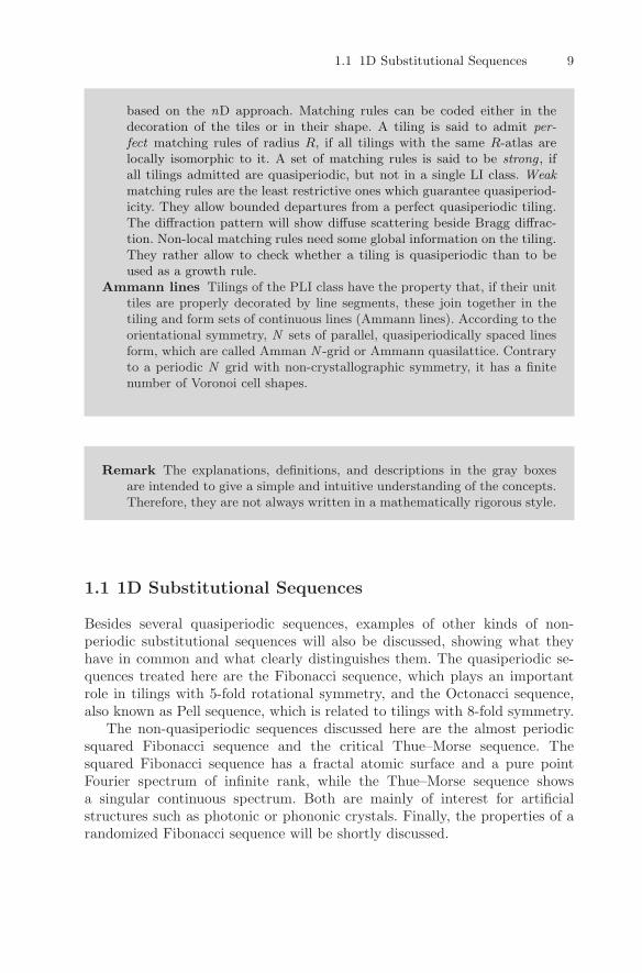
based on the nD approach. Matching rules can be coded either in thedecoration of the tiles or in their shape. A tiling is said to admit per-fect matching rules of radius R, if all tilings with the same R-atlas arelocally isomorphic to it. A set of matching rules is said to be strong , ifall tilings admitted are quasiperiodic, but not in a single LI class. Weakmatching rules are the least restrictive ones which guarantee quasiperiod-icity. They allow bounded departures from a perfect quasiperiodic tiling.The diffraction pattern will show diffuse scattering beside Bragg diffrac-tion. Non-local matching rules need some global information on the tiling.They rather allow to check whether a tiling is quasiperiodic than to beused as a growth rule.

Ammann lines Tilings of the PLI class have the property that, if their unittiles are properly decorated by line segments, these join together in thetiling and form sets of continuous lines (Ammann lines). According to theorientational symmetry, N sets of parallel, quasiperiodically spaced linesform, which are called Amman N -grid or Ammann quasilattice. Contraryto a periodic N grid with non-crystallographic symmetry, it has a finitenumber of Voronoi cell shapes.

Remark The explanations, definitions, and descriptions in the gray boxesare intended to give a simple and intuitive understanding of the concepts.Therefore, they are not always written in a mathematically rigorous style.

1.1 1D Substitutional Sequences

Besides several quasiperiodic sequences, examples of other kinds of non-periodic substitutional sequences will also be discussed, showing what theyhave in common and what clearly distinguishes them. The quasiperiodic se-quences treated here are the Fibonacci sequence, which plays an importantrole in tilings with 5-fold rotational symmetry, and the Octonacci sequence,also known as Pell sequence, which is related to tilings with 8-fold symmetry.

The non-quasiperiodic sequences discussed here are the almost periodicsquared Fibonacci sequence and the critical Thue–Morse sequence. Thesquared Fibonacci sequence has a fractal atomic surface and a pure pointFourier spectrum of infinite rank, while the Thue–Morse sequence showsa singular continuous spectrum. Both are mainly of interest for artificialstructures such as photonic or phononic crystals. Finally, the properties of arandomized Fibonacci sequence will be shortly discussed.


1.1.1 Fibonacci Sequence (FS)

The Fibonacci sequence, a 1D quasiperiodic substitutional sequence (see, e.g.,[26]), can be obtained by iterative application of the substitution rule σ : L �→LS,S �→ L to the two-letter alphabet {L, S}. The substitution rule can bealternatively written employing the substitution matrix S

σ :(

LS

)�→(

1 11 0

)

︸︷︷︸=S

(LS

)=(

LSL

). (1.1)

The substitution matrix does not give the order of the letters, just their rel-ative frequencies in the resulting words wn, which are finite strings of thetwo kinds of letters. Longer words can be created by multiple action of thesubstitution rule. Thus, wn = σn(L) means the word resulting from the n-thiteration of σ (L): L �→ LS. The action of the substitution rule is also calledinflation operation as the number of letters is inflated by each step. The FScan as well be created by recursive concatenation of shorter words accordingto the concatenation rule wn+2 = wn+1wn. The generation of the first fewwords is shown in Table 1.1.

The frequencies νLn = Fn+1, ν

Sn = Fn of letters L, S in the word wn =

σn(L), with n ≥ 1, result from the (n − 1)th power of the transposed substi-tution matrix to (

νLn

νSn

)= (ST )n−1

(11

). (1.2)

The Fibonacci numbers Fn+2 = Fn+1 + Fn, with n ≥ 0 and F0 = 0, F1 = 1,form a series with limn→∞ Fn/Fn−1 = τ = 1.618 . . ., which is called thegolden ratio. Arbitrary Fibonacci numbers can be calculated directly byBinet’s formula

Table 1.1. Generation of words wn = σn(L) of the Fibonacci sequence by repeatedaction of the substitution rule σ(L) = LS, σ(S) = L. νL

n and νSn denote the frequencies

of L and S in the words wn; Fn are the Fibonacci numbers

n wn+2 = wn+1wn νLn νS

n

0 L 1 01 LS 1 12 LSL 2 13 LSLLS 3 24 LSLLSLSL 5 35 LSLLSLSLLSLLS 8 56 LSLLSLSLLSLLS︸︷︷︸LSLLSLSL︸︷︷︸ 13 8

w5 w4

......

......

n Fn+1 Fn


τ−1Sτ−1L

L

τ−2L τ−2S τ−2L

Fig. 1.1. Graphical representation of the substitution rule σ of the Fibonacci se-quence. Rescaling by a factor 1/τ at each step keeps the total length constant. Shownis a deflation of the line segment lengths corresponding to an inflation of letters

Fn =(1 +

√5)n − (1 −

√5)n

2n√

5. (1.3)

The number τ If a line segment is divided in the golden ratio, then thisgolden section has the property that the larger subsegment is related to thesmaller as the whole segment is related to the larger subsegment (Fig. 1.1).This way of creating harmonic proportions has been widely used in art and ar-chitecture for millenniums. The symbol τ is derived from the Greek noun τoμηwhich means cut, intersection. Alternatively, the symbol φ is used frequently.τ can be represented by the simplest possible continued fraction expansion

τ = 1 +1

1 + 1

1+ 11+...

. (1.4)

Since it only contains the numeral one, it is the irrational number with theworst truncated continued fraction approximation. The convergents ci are justratios of two successive Fibonacci numbers

c1 = 1, c2 = 1 +1

1= 2, c3 = 1 +

1

1 + 11

=3

2, . . . , cn =

Fn+1

Fn. (1.5)

This poor convergence is the reason that τ is sometimes called the “mostirrational number.” The strong irrationality may impede the lock-in of in-commensurate (quasiperiodic) into commensurate (periodic) systems such asrational approximants.

The scaling properties of the FS can be derived from the eigenvalues λi of thesubstitution matrix S. For this purpose, the eigenvalue equation

det |S − λI| = 0, (1.6)

with the unit matrix I, has to be solved. The evaluation of the determinantyields the characteristic polynomial

λ2 − λ − 1 = 0 (1.7)


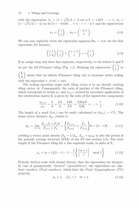
with the eigenvalues λ1 = (1 +√

5)/2 = 2 cos π/5 = 1.618 . . . = τ , λ2 =(1−

√5)/2 = −2 cos 2π/5 = −0.618 . . . = 1− τ = −1/τ and the eigenvectors

v1 =(

τ1

), v2 =

(−1/τ

1

). (1.8)

We can now explicitly write the eigenvalue equation Svi = λivi for the firsteigenvalue, for instance,

(1 11 0

)(τ1

)=(

τ + 1τ

)= τ

(τ1

). (1.9)

If we assign long and short line segments, respectively, to the letters L and S

we get the 1D Fibonacci tiling (Fig. 1.1). Relating the eigenvector(

τ1

)to

(LS

)shows that an infinite Fibonacci tiling s(r) is invariant under scaling

with the eigenvalue τ , s(τr) = s(r).The scaling operation maps each tiling vector r to an already existing

tiling vector τr. Consequently, the ratio of patches of the Fibonacci tiling,which correspond to words wn and wn+1 created by successive application ofthe substitution matrix S, is given by the ratio of the eigenvector components

wn+1

wn=

LS

=LSL

=LSLLS

=LSLLSLSL

= · · · =τ

1. (1.10)

The length of a word �(wn) can be easily calculated to �(wn) = τnL. Themean vertex distance, dav, results to

dav = limn→∞

Fn+1L + FnSFn+1 + Fn

=

{Fn+1

Fn+2τ +

Fn

Fn+2

}

S = (3 − τ)S, (1.11)

yielding a vertex point density Dp = 1/dav. dav = aPAS is also the period ofthe periodic average structure (PAS) of the FS (see section 3.3). The totallength of the Fibonacci tiling for n line segments reads, in units of S,

xn = (n + 1)(3 − τ) − 1 − 1τ

{[n + 1

τ

]mod 1

}

. (1.12)

Periodic lattices scale with integer factors, thus the eigenvalues are integers.In case of quasiperiodic “lattices” (quasilattices), the eigenvalues are alge-braic numbers (Pisot numbers), which have the Pisot–Vijayaraghavan (PV)property :

λ1 > 1, |λi| < 1 ∀i > 1. (1.13)


Thus, a Pisot number is a real algebraic number larger than one and itsconjugates have an absolute value less than one. Tilings satisfy the PV prop-erty if they have point Fourier spectra. The PV property connected to this isthat the n-th power of a Pisot number approaches integers as n approachesinfinity. The PV property is a necessary condition for a pure point Fourierspectrum, however, it is not sufficient. The Thue–Morse sequence, for instance,has the PV property, but it has a singular continuous Fourier spectrum (seeSect. 1.1.4).

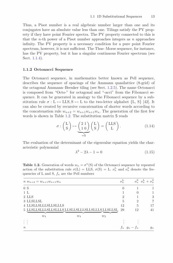
1.1.2 Octonacci Sequence

The Octonacci sequence, in mathematics better known as Pell sequence,describes the sequence of spacings of the Ammann quasilattice (8-grid) ofthe octagonal Ammann–Beenker tiling (see Sect. 1.2.5). The name Octonacciis composed from “Octo-” for octagonal and “-acci” from the Fibonacci se-quence. It can be generated in analogy to the Fibonacci sequence by a sub-stitution rule σ : L �→ LLS,S �→ L to the two-letter alphabet {L, S} [42]. Itcan also be created by recursive concatenation of shorter words according tothe concatenation rule wn+2 = wn+1wn+1wn. The generation of the first fewwords is shown in Table 1.2. The substitution matrix S reads

σ :(

LS

)�→(

2 11 0

)

︸︷︷︸=S

(LS

)=(

LLSL

). (1.14)

The evaluation of the determinant of the eigenvalue equation yields the char-acteristic polynomial

λ2 − 2λ − 1 = 0 (1.15)

Table 1.2. Generation of words wn = σn(S) of the Octonacci sequence by repeatedaction of the substitution rule σ(L) = LLS, σ(S) = L. νL

n and νSn denote the fre-

quencies of L and S, fn are the Pell numbers

n wn+2 = wn+1wn+1wn νLn νS

n νLn + νS

n

0 S 0 1 11 L 1 0 12 LLS 2 1 33 LLSLLSL 5 2 74 LLSLLSLLLSLLSLLLS 12 5 175 LLSLLSLLLSLLSLLLS︸︷︷︸LLSLLSLLLSLLSLLLS︸︷︷︸LLSLLSL︸︷︷︸ 29 12 41

w4 w4 w3

......

......

n fn gn − fn gn


with the eigenvalues λ1 = 1 +√

2 = (2 +√

8)/2 = 2.41421 . . . = ω, λ2 =1 −

√2 = −0.41421 . . ., which satisfy the PV property. The eigenvalue ω can

be represented by the continued fraction expansion

ω = 2 +1

2 + 12+ 1

2+...

. (1.16)

The frequencies νLn = fn, νS

n = gn −fn of letters L, S in the word wn = σn(S),with n ≥ 1, result to

(νL

n + νSn

νLn − νS

n

)= (ST )n−1

(11

). (1.17)

The Pell numbers fn+2 = 2fn+1 +fn, with n ≥ 0 and f0 = 0 and f1 = 1, forma series with limn→∞ fn+1/fn = 1+

√2 = 2.41421 . . ., which is called the silver

ratio or silver mean. They can be calculated as well by the following equation

fn =ωn − ω−n

ω − ω−1(1.18)

The 2D analogue to the Octonacci sequence, a rectangular quasiperiodic2-grid, can be constructed from the Euclidean product of two tilings thatare each based on the Octonacci sequence. If only even or only odd verticesare connected by diagonal bonds then the so called Labyrinth tilings Lm andtheir duals L∗

m, respectively, result [42].

1.1.3 Squared Fibonacci Sequence

By squaring the substitution matrix S of the Fibonacci sequence, the squaredFS can be obtained

σ :(

LS

)�→(

2 11 1

)

︸︷︷︸=S2

(LS

)=(

LLSSL

). (1.19)

This operation corresponds to the substitution rule σ : L �→ LLS,S �→ SLapplied to the two-letter alphabet {L, S}.

The scaling properties of the squared FS can be derived from the eigenval-ues λi of the substitution matrix S2. For this purpose, the eigenvalue equation

det |S2 − λI| = 0, (1.20)

with the unit matrix I, has to be solved. The evaluation of the determinantyields the characteristic polynomial

λ2 − 3λ + 1 = 0 (1.21)

with the eigenvalues λ1 = τ2, λ2 = 1/τ2 = 2 − τ , which satisfy the PVproperty, and the same eigenvectors as for the FS. The generation of the firstfew words is shown in Table 1.3.


Table 1.3. Generation of words wn = σn(L) of the squared Fibonacci sequence byrepeated action of the substitution rule σ(L) = LLS, σ(S) = SL or by concatenation.νL

n and νSn denote the frequencies of L and S in the words wn, Fn are the Fibonacci

numbers

n wn = wn−1wn−1wn−1, wn = wn−1wn−1 with w0 = L and w0 = S νLn νS

n

0 L 1 0

1 LLS 2 1

2 LLSLLSSL 5 3

3 LLSLLSSLLLSLLSSLSLLLS 13 8

4 LLSLLSSLLLSLLSSLSLLLS︸︷︷︸ LLSLLSSLLLSLLSSLSLLLS︸︷︷︸ SLLLSLLSLLSSL︸︷︷︸ 34 21

w3 w3 w3

.

.

....

.

.

....

n F2n+1 F2n

Table 1.4. Generation of words wn = σn(A) of the Thue–Morse sequence by re-peated action of the substitution rule σ(A) = AB, σ(B) = BA or by concatenation

n wn = wn−1wn−1, wn = wn−1wn−1 with w0 = A and w0 = B

0 A1 AB2 ABBA3 ABBABAAB4 ABBABAABBAABABBA5 ABBABAABBAABABBA︸︷︷︸BAABABBAABBABAAB︸︷︷︸

w4 w4

......

1.1.4 Thue–Morse Sequence

The (Prouhet-)Thue–Morse sequence results from the multiple application ofthe substitution rule σ : A �→ AB,B �→ BA to the two-letter alphabet {A, B}.The substitution rule can be alternatively written employing the substitutionmatrix S

σ :(

AB

)�→(

1 11 1

)

︸︷︷︸=S

(AB

)=(

ABBA

). (1.22)

The frequencies in the sequence of the letters A and B are equal. The length ofthe sequence after the n-th iteration is 2n. The Thue–Morse sequence can alsobe generated by concatenation: wn+1 = wnwn, wn+1 = wnwn with w0 = Aand w0 = B (Table 1.4).


The characteristic polynomial λ2−2λ = 0 leads to the eigenvalues λ1 = 2 andλ2 = 0. Although these numbers show the PV property, the Fourier spectrumof the TMS can be singular continuous without any Bragg peaks. If we assignintervals of a given length to the letters A and B, then every other vertexbelongs to a periodic substructure of period A+B. This is also the size of theunit cell of the PAS, which contains two further vertices at distances A andB, respectively, from its origin. All vertices of the PAS are equally weighted.The Bragg peaks, which would result from the PAS, are destroyed for specialvalues of A and B by the special order of the Thue–Morse sequence leadingto a singular continuous Fourier spectrum. The broad peaks split into moreand more peaks if the resolution is increased. In the generic case, however,a Fourier module exists beside the singular continuous spectrum. Dependingon the decoration, the Thue–Morse sequence will show Bragg peaks besidesthe singular continuous spectrum (see Fig. 6.2).

1.1.5 1D Random Sequences

It is not possible to say much more about general 1D random sequences thanthat their Fourier spectra will be absolutely continuous. However, dependingon the parameters (number of prototiles, frequencies, correlations), the spectracan show rather narrow peaks for particular reciprocal lattice vectors. Generalformulas have been derived for different cases of 1D random sequences [15].

The diffraction pattern of a FS, decorated with Al atoms and randomizedby a large number of phason flips, is shown in Fig. 1.2. Although the Fourierspectrum of such a random sequence is absolutely continuous, it is peaked forreciprocal space vectors of the type m/L and n/S with m ≈ nτ , with m andn two successive Fibonacci numbers.

The continuous diffuse background under the peaked spectrum of the ran-domized FS can be described by the relation Idiff ∼ f(h)[1− cos(2πh(L− S)](fAl(h) is the atomic form factor of Al, L, and S are the long and short inter-atomic distances in the Al decorated FS).

1.2 2D Tilings

The symmetry of periodic tilings, point group and plane group (2D spacegroup), can be given in a straightforward way (see, e.g., Table 1.7). In case ofgeneral quasiperiodic tilings, there is no 2D space or point group symmetryat all. Some tilings show scaling symmetry. In case of singular tilings, there isjust one point of global point group symmetry other than 1. The orientationalorder of equivalent tile edges (“bond-orientational order”), however, is clearlydefined and can be used as one parameter for the classification of tilings. Thismeans, one takes one type of tile edge, which may be arrowed or not, in allorientations occurring in the tiling and forms a star. The point symmetrygroup of that star is then taken for classifying the symmetry of the tiling.

1.2 2D Tilings 17

Inte

nsity

(lo

garit

hmic

)

0 0.1 0.2 0.3 0.4 0.5 Å-1

Fig. 1.2. Diffraction patterns of a Fibonacci sequence before (top) and after (bottom)partial randomization (≈ 25% of all tiles have been flipped). The vertices of theFibonacci sequence are decorated by Al atoms with the short distance S = 2.4 A; thediffraction patterns have been convoluted with a Gaussian with FWHM = 0.001 A−1

to simulate realistic experimental resolution (courtesy of Th. Weber)

Table 1.5. Point groups of 2D quasiperiodic structures (tilings) (based on [13]).Besides the general case with n-fold rotational symmetry, a few practically relevantspecial cases are given. k denotes the order of the group

Point group type k Conditions n = 5 n = 7 n = 8 n = 10 n = 12 n = 14

nmm 2n n even 8mm 10mm 12mm 14mm

nm 2n n odd 5m 7m

n n 5 7 8 10 12 14

This is related to the autocorrelation (Patterson) function. In Table 1.5, thepossible point symmetry groups of 2D quasiperiodic structures (tilings) aregiven.

The general space group symmetries possible for 2D quasiperiodic struc-tures with rotational symmetry n ≤ 15 are listed in Table 1.6.

By taking the symmetry of the Patterson function for the tilingsymmetry, it is not possible to distinguish between centrosymmetric andnon-centrosymmetric tilings. This means that in the case of 2D tilings only

springerseriesin materialsscience...

Documents