spherical bubble dynamics in a bubbly medium using … · surrounding bubbly medium and how it...
TRANSCRIPT

Accepted by Chemical Engineering Science 10.1016/j.ces.2015.01.056
* Corresponding author.
Emails: [email protected]; [email protected]; [email protected]
Phone: 301-604-3688
Fax: 301-604-3689
Spherical Bubble Dynamics in a Bubbly Medium using
an Euler-Lagrange Model
Jingsen Maa,*, Georges L. Chahine
a , and Chao-Tsung Hsiao
a
aDYNAFLOW, INC., 10621-J Iron Bridge Road, Jessup, MD, USA
Abstract
For applications involving large bubble volume changes such as in cavitating flows and
in bubbly two-phase flows involving shock and pressure wave propagation, the
dynamics, relative motion, deformation, and interaction of bubbles with the surrounding
medium play crucial roles and require accurate modeling. We present in this paper a
fundamental study of the dynamic oscillations of a ‘primary’ bubble in a bubbly mixture
using a two-way coupled Euler-Lagrange model. It addresses a simplified spherical
configuration while using the full three-dimensional code. A main objective of the study
is to investigate how the dynamics of a ‘primary’ bubble is affected by the presence of a
surrounding bubbly medium and how it differs from its behavior in a pure liquid. This
helps elucidate the physics at play for this relatively simple configuration. The model
simulates the mixture as a continuum and solves the corresponding Navier Stokes
equations with grids moving with the interface of the primary bubble wall. The
surrounding microbubbles are tracked in a Lagrangian fashion accounting for their
volume evolution. The two-way coupling between the bubbly medium and the primary

2 J. Ma, G.L. Chahine, and C.-T. Hsiao
bubble dynamics is realized through the local density of the mixture obtained from the
tracking of the microbubbles and the determination of their volumes and spatial
distribution.
The simulations clearly indicate that the surrounding microbubbles absorb energy
emitted from the primary bubble during its oscillations. This results in a reduction of the
maximum radius and the period of oscillations of the primary bubble as compared to the
dynamics in the pure liquid. Also, accounting for the dynamics of the field bubbles
brings out the presence in the two-phase medium of a phase shift between density and
pressure distributions. Such a shift is not captured by two-phase homogeneous medium
models. These effects increase with increase in the mixture void fraction and in the
initial bubble sizes in the mixture. The numerical observations are found to be in good
qualitative agreements with previously published experimental data (Jayaprakash et al.,
2011) investigating spark generated bubble dynamics in a bubbly medium.
Key Words: Bubble Dynamics, Bubbly Medium, Euler-Lagrange Model, Two-way
Coupling, Phase Shift
1. INTRODUCTION
Bubbly flows are prevalent in chemical engineering processes and there are many
engineering systems, where the dynamics of clouds of vapor or gas bubbles is of
fundamental importance. For example, bubble columns reactors are used in a wide
spectrum of chemical and energy applications (van Sint Annaland et al., 2005, Darmana
et al., 2007, Law et al., 2008, Chen et al., 2009), with typical examples including
Fischer-Tropsch synthesis (Guillen et al., 2011), methanol and dimethylether syntheses
(Wu & Gidaspow, 2000), coal liquefaction (Law et al., 2007, Law et al., 2011), or algae
Bubble in bubbly medium 3
3
bioreaction (Singh & Sharma, 2012) etc. Also, nucleate pool boiling is applied in
different industrial processes such as distillation or thermal transport (Arndt, 1981,
Blake & Gibson, 1987). In addition, pipes containing air ventilated cavities are
frequently encountered in engineering facilities including airlift bioreactors or U-tube
fermenters (Xiang et al., 2011, Xiang et al., 2014). The use of cavitation for the
intensification of bio-chemical processes is also very common such as in surface
cleaning (Ohl et al., 2006), bacteria disinfection processes (Johnson et al., 1982,
Kalumuck et al., 2003, Loraine et al., 2012), or biomedical therapy applications
(Coleman et al., 1987, Zhong et al., 2001, Kennedy, 2005, Mitragotri, 2005, Chung &
Cho, 2009, Capretto et al., 2011, Yuan et al., 2011, Chahine & Hsiao, 2012, Hsiao et al.,
2013a, Madadi-Kandjani & Xiong, 2014). Most of these above-mentioned problems
involve large bubble volume changes due to boiling, cavitation and/or bubble breakup
and coalescence. Particularly, in liquid phase oxidation processes such as injection of
oxygen into liquid (Kalumuck & Chahine, 2000) an explosion behavior occurs,
followed by the emission of high-peak spherical pressure waves which propagates
through the surrounding bubbly liquid. In these kinds of problems, shock and pressure
wave propagation in bubbly media, the dynamics, relative motion, and interaction of
bubbles with the surroundings play crucial roles on the process in question and require
accurate modeling, which poses fundamental challenges.
Since the early works of Besant (1859) and Rayleigh (1917) a large body of
literature has been devoted to the dynamics of spherical bubbles. Plesset (1949)
presented a comprehensive model describing the time variations of the radius of a

4 J. Ma, G.L. Chahine, and C.-T. Hsiao
bubble containing compressible gas in an incompressible liquid when the liquid is
subjected to a time dependent ambient pressure. The model conserves mass and
momentum, includes surface tension and liquid viscous effects, but ignores gas diffusion
and heat transfer between the bubble and the liquid. Since then, many researchers have
extended this model to include other effects such as liquid compressibility (Herring,
1941, Gilmore, 1952, Keller & Kolodner, 1956, Prosperetti & Lezzi, 1986, Prosperetti,
1987), mass transfer (Prosperetti, 1982, Hsiao & Chahine, 2012), heat transfer (Miksis
& Ting, 1984, Chahine & Liu, 1985, Prosperetti et al., 1988, Commander & Prosperetti,
1989, Prosperetti, 1991), electro-potential effects (Oh et al., 2001, Spelt & Matar, 2006),
magnetic effects (Yasui, 1999, Aliabadi & Taklifi, 2012). Even though not directly
applicable to the present study, several models have also been developed and applied to
the study of non-spherical bubble dynamics (Chahine, 1982, Zhang et al., 1993, Hsiao
& Chahine, 2001, Choi et al., 2009, Wang & Blake, 2010). The Rayleigh-Plesset
equation (Rayleigh-Plesset equation) and its small compressibility equivalent models
(Herring, 1941, Gilmore, 1952, Keller & Kolodner, 1956), remain however, by far the
most widely used models for a wide range of applications involving bubble dynamics
such as hydrodynamic cavitating flows (Plesset, 1949, Ceccio & Brennen, 1991,
Brennen, 1995, Chahine, 2009, Brennen, 2011), acoustic cavitation applications (Keller
& Miksis, 1980, Hilgenfeldt et al., 1998, Moholkar et al., 1999, Prosperetti & Hao,
1999, Calvisi et al., 2007), two-phase bubbly flows (Seo et al., 2010, Shams et al., 2011,
Hsiao et al., 2013b), and underwater explosion bubbles (Herring, 1941, Keller &
Kolodner, 1956, Chahine & Harris, 1997, Wardlaw & Mair, 1998, Geers & Hunter,
2002, Krieger & Chahine, 2005, de Graaf et al., 2012). This is predominantly because
of the success of these methods at recovering the key physics involved in each
application and because of the simplicity of their implementation as compared to other
models.
The incompressible Rayleigh-Plesset equation actually remains at the core of the
solutions of most numerical simulation models of two-phase bubbly flows (Plesset &
Prosperetti, 1977). In most cases, as for the classical modeling of a two-phase flow in a

Bubble in bubbly medium 5
5
nozzle, an equivalent medium approach is used with the equivalent density determined
from the volume occupied by the bubbles and obtained with simplifying assumptions
through local solution of the Rayleigh-Plesset equation (Van Wijngaarden, 1964,
Brennen, 1995, Grandjean et al., 2012). In general, two-phase bubbly flows are modeled
using one of the following approaches: an equivalent homogeneous continuum
approach, an Eulerian two-fluid approach, or an Eulerian-Lagrangian approach wherein
the bubbles are treated as discrete particles. While homogeneous models, which are
useful for low void fraction and very small bubble oscillations conditions, ignore bubble
dynamics and do not require Rayleigh-Plesset equation solutions, the other two
approaches do require such modeling. Eulerian-Lagrangian approaches are more
appropriate for higher void fractions (Spelt & Biesheuvel, 1997, Balachandar & Eaton,
2010, Raju et al., 2011, Shams et al., 2011). In a recent work by Raju et al. (2011)
comparing a continuum homogeneous model (Gilmore, 1952) , an Eulerian multi-
components model (Wardlaw & Luton, 2000, Wardlaw & Luton, 2003), and an
Eulerian-Lagrangian model (Hsiao et al., 2003, Chahine, 2009, Hsiao et al., 2013b) it
was found that high-frequency local fluctuations were only captured when an Eulerian
viscous solver was coupled with a Lagrangian discrete bubble dynamics and when the
microscale behavior of the field bubbles was well resolved. Continuum models, on the
other hand, captured well the average low-frequency behavior. Proper discrete bubble
modeling is thus essential to an accurate modeling of the problem (Sussman, 2003,
Francois et al., 2006, Fuster & Colonius, 2011, Lauer et al., 2012, Aanjaneya et al.,
2013, Arienti & Sussman, 2014).
In this paper, we utilize a generalized 3D two-way coupled Euler-Lagrange two-
phase flow model and apply it in a spherical configuration to study the dynamics of a
primary bubble oscillating in a bubbly mixture. The 3D model has been developed to
study bubbly and cavitating flows such as the effects of a propeller flow and dissolved
gas diffusion into and out of the bubbles on the bubble size distribution in water (Hsiao
& Chahine, 2012), the development of tip vortex cavitation on propellers (Hsiao &
Chahine, 2008), bubbly flow in a bubble augmented propulsor (Wu et al., 2010), bubble

6 J. Ma, G.L. Chahine, and C.-T. Hsiao
entrainment in jet wake flows (Hsiao et al., 2013b), and has evolved from the study of
highly deformable bubbles in vortices (Hsiao & Chahine, 2001, Choi et al., 2009) and
cavitating flow (Chahine & Hsiao, 2000, Chahine, 2009).
The 3D two-phase mixture domain is gridded using an O-grid with a moving grid
adapting to the moving primary bubble wall boundary. The equivalent continuum
Navier-Stokes equations with local and time dependent local void fractions are solved in
this domain. The shape of the surrounding bubbles is not the subject of particular
attention in this study and these bubbles are treated in an approximated manner as
singularities with the first mode being a source with its intensity satisfying the Rayleigh-
Plesset-Keller-Herring equations. Deformation of these bubbles is ignored, however
volume change, motion and interactions, and their effects on the flow are well captured.
The two-way coupling between the mixture flow and the dispersed bubbles is realized
through the local mixture density, which is based on continual updating of the local
volume and distribution of the dispersed bubbles. A Gaussian scheme is adopted to
smooth the void fraction spatial distribution and derivatives. Using this model, the
effects of the presence of the bubbles on the primary bubble dynamics and on the
propagation of pressure and density waves in the medium are investigated. Various
mixture conditions with void fractions ranging between 0% and 5% and field bubble
sizes between one tenth and one fifth of the primary bubble size are studied. The
configuration of the 3D problem is made practically spherically-symmetric by randomly
distributing the field bubbles in a spherical computational domain while satisfying a
statistically uniform void fraction distribution in space. This is for model verification
purposes and to facilitate comparison with available analytical spherical bubble
solutions. The model is however fully 3D and is not configuration limited. It is, for
instance, also suitable to study non-spherical bubble dynamics (e.g., bubble collapse
near a wall) in bubbly mixtures, which is illustrated briefly in the verification part of this
paper and which will be the subject of a separate paper.
The paper is organized as follows. In the next section we describe the main features
of the coupled Euler-Lagrange model, the void fraction computation method, and the

Bubble in bubbly medium 7
7
void distribution smoothing scheme. We then present the bubble driven flow considered
here and the results obtained using the simulation model, along with detailed
discussions of field bubble effects on the primary bubble dynamics and on the wave
propagation in the two-phase medium. Finally, we summarize the main findings from
the study.
2. EULER-LAGRANGE TWO-PHASE MODEL
2.1. Viscous Mixture Flow Solver
The two-phase bubbly mixture with gas volume fraction, , is treated as a
homogenous mixture with the following properties. The density, ρm, and kinematic
viscosity, m , are defined respectively as:
1 ,
1 ,
m l g
m l g
(1)
where ρg, and g , are respectively the density and kinematic viscosity of the gas, and
ρl, and l , are respectively the liquid density and kinematic viscosity.
Following the theoretical work on dilute bubbly flows of van Wijngaarden (1968,
1972), Commander & Prosperetti (1989) and Brennen (2005), the unsteady continuity
and momentum conservation equations for the liquid-gas homogeneous mixture are as
follows:
0,m
mt
u
(2)
2 ,m m m
Dp
Dt
uu g (3)
where t is time, is the mixture velocity, p its pressure, and is a body force such as
the acceleration of gravity Note that Equations (2) and (3) are written for the mixture
and not for the liquid. A different formulation is available in the literature, e.g. Ferrante
& Elghobashi (2004), Darmana et al. (2006), Shams et al. (2011), and applies the Navier
Stokes equations to the liquid (not the mixture) and, as a result, requires an additional
u g

8 J. Ma, G.L. Chahine, and C.-T. Hsiao
momentum exchange term. Here, a separate computation of the bubble motion and the
drag force is conducted.
Equations (2) and (3) are solved using the flow solver 3DYNAFS-VIS©
, formerly
called DFI-UNCLE (Hsiao & Chahine, 2001), which is based on the artificial-
compressibility method (Chorin, 1967), where a derivative of the pressure in the pseudo
time, , is added to (2) as:
1
0,mm
p
t
u (4)
where is an artificial compressibility factor. Equations (3) and (4) form a hyperbolic
system of equations and are solved using a time marching scheme in the pseudo-time,
. The time variations of the density is enforced as source terms in (3) and (4). To obtain
a time-dependent solution, a Newton procedure where pseudo-time iterative stepping in
is used at each physical time step, t, enables one to satisfy the continuity equation.
The numerical scheme uses a finite volume formulation. A first-order Euler
implicit difference scheme is applied to the time derivatives. The spatial differencing of
the convective terms uses a flux-difference splitting scheme based on Roe’s method
(Roe, 1981) and a van Leer’s MUSCL method (Anderson et al., 1986, Van Leer et al.,
1987) to obtain the first or third-order fluxes. A second-order central differencing is used
for the viscous terms and the flux Jacobians are obtained numerically. The resulting
system of algebraic equations is solved using a discretized Newton relaxation method in
which symmetric block Gauss-Seidel sub-iterations are performed before the solution is
updated at each Newton iteration. The 3DYNAFS-VIS©
solver has been extensively
validated and used to study a range of two-phase problems and its results have
compared favorably with available experimental data (Chahine et al., 2008, Chahine,
2009, Hsiao et al., 2010).
2.2. Lagrangian Modeling of Dispersed Phase
The bubbles dispersed in the field to form the two-phase medium are treated as point
sources and dipoles to account for their volume change and translation relative to the

Bubble in bubbly medium 9
9
liquid. Volume variations are obtained with a bubble dynamics equation using bubble
surface averaged pressures and velocities, to account for flow non-uniformities, and an
additional pressure term to account for bubble motion relative to the liquid (Hsiao et al.,
2003, Chahine, 2009). The equivalent spherical bubble radius, R(t), is obtained using a
modified Rayleigh-Plesset-Keller-Herring equation (Plesset & Prosperetti, 1977,
Prosperetti & Lezzi, 1986) which accounts for the compressibility of the surrounding
bubbly medium and for flow field non-uniformities:
0
2
3
0
31 (1 )
2 3 4
1 21 4 ,
enc
enc
b
m m
k
v g m
m m m
R RRR R
c c
RR R d Rp p p
c c dt R R R
u u
(5)
where is the local sound speed in the two-phase medium, γ is the surface tension,
and pv is the vapor pressure. is the initial gas pressure in the bubble corresponding
to the initial bubble equivalent radius, R0. penc and uenc, the “encountered” pressure and
velocity respectively, are the pressures and velocities in the two-phase medium averaged
over the bubble surface. ub is the bubble translation velocity. The introduction of uenc
and penc in Equation (5) is to account for non-uniform pressures and velocities around
the bubble and for slip velocity between the bubble and the host medium. Using penc and
uenc instead of the conventionally used values at the bubble center, results in a major
improvement over classical models (Hsiao et al., 2003, Chahine, 2009). We will
concentrate here on purely inertial bubbles as for cavitation in liquid at ambient
temperatures (Brennen, 1995) and ignore gas diffusion and heat transfer. Including
these will be presented in other publications following our previous work as in (Chahine
& Liu, 1985). In “cold” liquids such as water at 20C, liquid vaporization occurs at a
much smaller time scale than the bubble dynamics scale, vapor goes in and out of the
bubble almost instantaneously, and the vapor inside the bubble remains constant and
equal to the liquid vapor pressure at the considered temperature. On the other hand, the
time scale of gas diffusion is very much larger than the bubble period and the amount of
mc
0gp

10 J. Ma, G.L. Chahine, and C.-T. Hsiao
gas inside the bubble remains the same, which allows one to use the compression law
with the constant k in Equation (5).
The bubble trajectory is obtained using the following equation of motion of the
bubble in the liquid flow, which extends the (Johnson & Hsieh, 1966) equation by
adding a lift force on the bubble,
3 32 +
4
3 3,
2
enc enc
b Db b
l
enc blLenc b
l
d Cp g
dt R
CR
R R
uu u u u
u u ωu u
ω
(6)
where is the local vorticity, CL is the lift coefficient, and CD is the drag coefficient
given by (Haberman & Morton, 1953):
0.63 4 1.38224
1 0.197 2.6 10 , .encl b
D eb eb eb
eb l
RC R R R
R
u u
(7)
The last term in the right hand side of (6) is the Bjerknes force (Bjerknes, 1906) term
due to coupling between bubble volume variations and bubble motion.
2.3. Eulerian-Lagrangian Coupling
The two-way coupling between the Eulerian continuum-based model and the
Lagrangian discrete bubble model is realized through the following steps:
The volume change of the individual bubbles in the flow field are controlled by the
two-phase medium local properties and flow field gradients.
The bubble motion in the flow field is controlled by the liquid flow field.
The local properties of the mixture (void fractions and local densities) are
determined by the spatial distribution of the bubble and by their volumes.
The mixture flow field with evolving mixture density distribution satisfies mass
and momentum conservation.
ω

Bubble in bubbly medium 11
11
The key to this coupling scheme is the deduction of a void fraction distribution from
the instantaneous bubble sizes and locations. Initially, the void fraction was defined in
each computational cell as the ratio of the total volume of bubbles in the cell by the cell
volume. However, this was found not totally satisfactory because it often resulted in
difficulty with differentiation due to the non-continuous character of α across cells (Wu
et al., 2010, Raju et al., 2011)
Here, to smooth the discontinuities and improve stability, we apply a Gaussian gas
volume distribution scheme to smoothly “spread” a bubble volume across neighboring
cells as in (Kitagawa et al., 2001, Darmana et al., 2006, Shams et al., 2011, Capecelatro
& Desjardins, 2013). As illustrated in Figure 1, the void fraction computation scheme
for a representative cell i is obtained using the following expression:
,
1
,
,i
cells
bNi j j
i Nj cell
k j k
k
f V
f V
(8)
where b
jVand
cell
kVare the volumes of the bubble j and the cell k, respectively. Ni is the
total number of bubbles which are in the “influence range” of the cell i. Ncells is the total
number of cells “influenced” by bubble j, and fi,j is the weight factor of the contribution
of bubble j to cell i based on distance. The weight factor is provided by the Gaussian
distribution function:
, 3
2| |
221
,( 2 )
i j
ij
sf eS
X
(9)
where |Xi,j| is the distance between bubble j and the center of cell i, and S is the standard
deviation. The derivation of the above expression (8) can be obtained as follows. The
void contribution of a bubble j to a neighboring cell k can be obtained first by uniformly
distributing the bubble volume to all the neighboring cells. This gives for the first
approximation of the volume fraction due to bubble j in cell k:

12 J. Ma, G.L. Chahine, and C.-T. Hsiao
,0 .cells
b
j
k Ncell
k
k
Va
V
(10)
However, for a closer representation of the actual physics, the cells nearer to a given
bubble should receive a larger contribution. To do so, we adjust (10) by using a weight
function dependent on the distance between the bubble center and the cell center. This is
achieved through the use of the Gaussian function in Equation (9). The modified
approximation of the volume fraction due to bubble j in cell k then becomes:
,1 , .cells
b
j
k k jNcell
k
k
Va f
V
(11)
However, does satisfy conservation of the redistributed gas volume in the
computational domain. To conserve the gas mass, we need to multiply by a
normalization factor, Wk, defined as the ratio of the volume of the bubble to the total
gas volume in all cells, Ncells , i.e.,
,,
,
( ) ( )( )
cells
cells cellscells
cells
Ncell
b b kj j k
k N b NNcell celljcell
k k k k jk k jNk kcellk
k
k
VV V
WV
V V fV f
V
(12)
This gives us the final expression of the volume fraction due to bubble j in cell k:
,
,
.
( )cells
b
j
k k jNcell
k k j
k
Va f
V f
(13)
Finally, adding up the effects of all the Ni bubbles influencing cell i , one obtains
readily Equation (8) from Equation (13).
,1ka
,1ka

Bubble in bubbly medium 13
13
Figure 1. Illustration of the void fraction computation using the Gaussian distribution
scheme.
2.4. Primary Bubble Surface-Tracking Method
In this study we consider conditions where the dynamics of the two-phase medium
and of the dispersed bubbles are driven by the “primary” bubble behavior. In this case,
it is essential to fully resolve the wall motion of this primary bubble and the high
pressure and velocity gradients near it. Even though the physical problem considered
here for verification purposes is spherical, a full 3D approach is taken. This allows to
readily consider more complex configurations next. To do so, an explicit surface-
tracking method using a moving grid technique is implemented and kinematic and
dynamic free surface boundary conditions are imposed at the bubble-liquid interface.
The Navier-Stokes equations are solved in the liquid domain containing the distributed
field bubbles constrained by the free-surface boundary conditions at the primary bubble
interface.
i
j
Bubble “gas volume” contribution range

14 J. Ma, G.L. Chahine, and C.-T. Hsiao
The kinematic condition expresses that a fluid particle at the bubble-liquid interface
remains on that surface. Specifically, if we define the equation of the free surface
through the scalar function F,
, , , 0,iF t H t (14)
where , ,i t are the curvilinear coordinates with being in the direction normal
to the bubble surface. The kinematic boundary condition can be written:
0ii
DF F FU
Dt t
, (15)
where , ,iU U V W are the contravariant velocity components.
Combining the equations (14) and (15) provides the general kinematic boundary
condition in curvilinear coordinates as
H H H
W U Vt t
. (16)
The free surface dynamic boundary condition imposed at the bubble surface include
balance of the normal stresses and vanishing shear stresses since we neglect the shear
due to the gas inside the bubble. By requiring the grid to be normal to the interface
boundary and assuming that the tangential derivatives of the normal velocity to the
interface, , are negligible relative to the other derivatives, we use
the Batchelor (1967) and Hodges et al. (1996) simplification to obtain:
0
0U
, (17)
0
0V
, (18)
0
g v m m
Wp p p gz
C (19)
where p is the liquid pressure at the bubble surface, pg and pv are the gas and vapor
pressure inside the bubble respectively, and is the interface curvature.
/ and /W W
C

Bubble in bubbly medium 15
15
A combination of algebraic and elliptic grid generation techniques (Hsiao, 1996,
Hsiao & Pauley, 1998) is used to update the position of the moving grid as the primary
bubble changes volume and the interface points move away from or towards the origin.
The algebraic technique allows clustering and boundary-orthogonal grids near the
bubble surface. This is important for resolving the flow field near the bubble wall and
for properly applying the free surface boundary conditions. In addition, the elliptic grid
generation techniques smooth out any roughness resultant from the algebraic technique
and improve numerical stability.
3. SIMULATION SETUP
A primary bubble of radius R0 is placed in a bubbly mixture composed of randomly
distributed bubbles in an open 3D domain to create an initial quasi uniform void fraction
distribution in space (Figure 2). In this paper, we will consider cases with field bubbles
of the same size. This is not a constraint in the actual software and is used here only to
simplify the presentation of the results. This setup resembles previously studied
spherical bubble clouds (Mørch, 1981, Chahine, 1983, Chahine & Liu, 1985, Chahine &
Duraiswami, 1992, Brennen, 1995, Ma et al, 2015). However, one notable difference is
that here the central bubble (primary bubble) acting as the motion/pressure source is the
initial driver of the motion. It then responds to the behavior of the surrounding bubbles.
This also corresponds to our experimental tests of a spark generated bubble in a bubbly
medium (Jayaprakash et al., 2011). In this study, the other bubbles’ effects are included
through their locations and volume changes while shape effects are ignored. These
effects can be included, using the same code, at a much larger computational cost (Hsiao
& Chahine, 2001, Chahine, 2009, Choi et al., 2009, Hsiao et al., 2010).

16 J. Ma, G.L. Chahine, and C.-T. Hsiao
Figure 2: Schematic showing the problem configuration of an oscillating primary bubble in
a bubbly mixture (Left), and grid used for the solution of the Eulerian two-phase flow mixture
(Right). Note that the bubble interface and the grids are recomputed at each time step.
To study the dynamics of a spherical bubble cloud configuration we zero the gravity
term in the input to prevent the gravity body force from altering the spherical symmetry.
An O-O type single block grid is used as illustrated in Figure 2. The selected liquid
interface discretization of the primary bubble has 41 x 21 nodes and the fluid domain
has 25 nodes distributed in the radial direction between r = R0 and the radius of the
computational domain selected to be 100 R0. The grid in the radial direction is clustered
near the bubble surface. This grid has been shown to be fine enough to provide grid-
converged solutions for problems similar to that studied here (Raju et al., 2011). In the
far field a discretized boundary is used at r= A R0 and a zero-gradient condition is
imposed. A value of A=100 was found acceptable as illustrated in Figure 3. This
considers the problem of a primary bubble of initial radius R0 = 5 mm and initial gas
pressure Pg0 = 2 atm released in a bubbly mixture initially in equilibrium with the liquid
ambient pressure Pamb= 1 atm of water. The initial conditions of pressure and velocity in
the medium outside the primary bubble correspond to quiescent conditions, i.e., P=Pamb,
u=0. Figure 3 shows that changing the limit of the domain size from 100 R0 to 300 R0
Bubble in bubbly medium 17
17
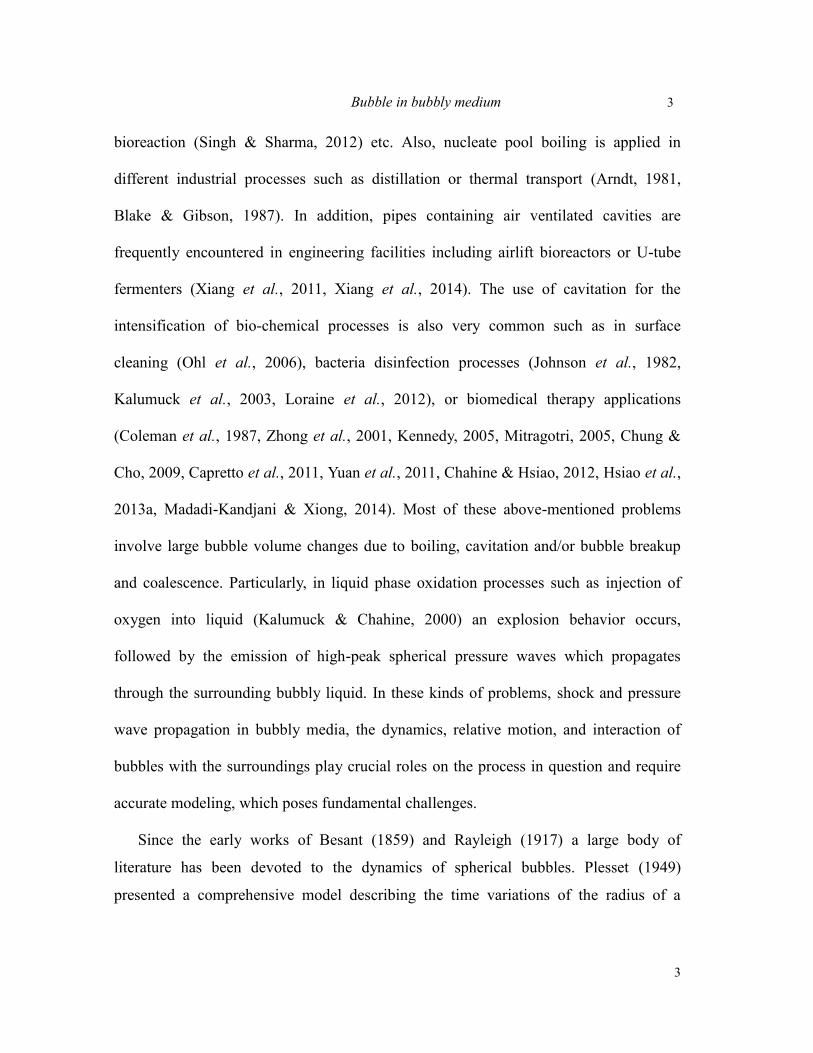
does not affect the solution in any significant fashion. The value 100 R0 is therefore used
for the following computations.
Figure 3: Effect of the domain size on the primary bubble radius versus time for the case of
R0 = 5 mm, Pg0 =2 atm, α0 = 1% and a0 = 1 mm.
We consider below the behavior of this bubbly medium and of the primary bubble
for initial void fractions, , ranging from 0 to 5% and for initial radii, , and for three
field bubbles initial uniform radii: 0.5, 0.75 and 1 mm. The bubbles are filled of air with
density is 1.2 kg/m3 and the file bubbles are considered in equilibrium at the initiation of
the computations and have an initial gas pressure given by 0 02 / ,g amb vP P a p
where ambP is the liquid ambient pressure, is the surface tension parameter with the
value used in the numerical computations, and pv is the vapor pressure
with the value pv =2,300 Pa. The initial bubble wall and translation velocities are all set
to zero.
For all the simulations presented in this paper, the artificial compressibility factor
in Equation (4) is chosen to be 200, which was found to be large enough to achieve
parameter independency, i.e., further increase of does not affect the simulation results.
This is illustrated in Figure 4a, which shows the effect of on the primary bubble
0 0a
0.0728 /N m

18 J. Ma, G.L. Chahine, and C.-T. Hsiao
equivalent radius. The results are seen to have already practically converged for
and to not change much for larger than 100. The solutions can also obviously be
affected by the selected size of the time steps – here not selected to be adaptive for
better understanding of the effect of the numeerical procedures. The effect of the time
step size, t, is shown in Figure 4b. The solutions overlap for time steps smaller than
3 μs, which correspond to , where by analogy to the Rayleigh collapse
time of an bubble of initial size R0, we define a RayleighT , which corresponds to the full
period of a gaseous bubble of initial size R0, in a liquid of density l , and an initial
positive pressure difference between the initial gas pressure in the bubble, , and the
ambient pressure, Pamb,
0
0
2 .lRayleigh
g amb
T RP P
(20)
Based on the above, a value of t=1.5 μs is selected for the verification study illustrated
below in Figure 4 and all the simulations presented hereafter.
Figure 4: Effect of the numerical parameters in the viscous problem solution on the primary
bubble radius versus time. (Left) Effect of the artificial compressibility parameter in Equation
(4). (Right) Effect of the time step size on convergence. R0 = 5 mm, Pg0 =2 atm. Bubbly
mixture conditions: α0 = 1% and a0 = 1 mm
/ 350Rayleight T
0gP

Bubble in bubbly medium 19
19
3.1. Shape of the primary bubble
Since the primary bubble and surrounding bubbly medium were selected to simulate
a spherical bubble behavior while the code used is fully three-dimensional, it is useful
to examine any deviation with time of the resulting primary bubble shape from a sphere.
The shape of the primary bubble at three instants during the dynamics is shown in
Figure 5 for the base case considered here (R0 = 5 mm, Pg0 = 2 atm, Pamb= 1 atm, initial
void fraction, = 1.0%, and initial “field” bubble radius a0 = 1 mm). The figure
indicates a visually very smooth spherical bubble shape at the three selected instances
during the bubble period: t = 0, t = 0.5 T0, and t = T0.
Figure 5: Primary bubble shape at different times during the first period of oscillations: (a)
t=0, (b) t=0.5T and (c) t=1.0T. = 1.0%, a0 = 1 mm, R0 = 5 mm, Pg0 = 2 atm, Pamb= 1 atm.
This is further demonstrated quantitatively in Figure 6a which compares the
temporal variations of the coordinates of four selected points on the bubble surface (at
X=Y=0 and X=Z=0). The four points appear to very closely follow the same dynamics.
Figure 6b shows the deviation of the radial distances of the four points from the
equivalent bubble radius, their averaged value versus time. We can see that these
deviations do not exceed 0.23%, which clearly indicates that the bubble remains very
close to a sphere. These minor deviations are due to the non-perfectly spherically
symmetric configuration generated by the random distribution of field bubbles. This
facilitates the comparative analysis of the simulation with analytical equations such as
0
0
t = 0 t = 0.5 T0 t = T0
D
B
C A

20 J. Ma, G.L. Chahine, and C.-T. Hsiao
the Gilmore equation which only deals with spherical bubble dynamics. Thus, any
differences found between the two methods should be attributed to the inclusion of the
individual field bubble dynamics in the modeling presented here, which plays no role in
homogenous medium analytical methods.
Figure 6 : (a) Temporal variation of the coordinates of the four representative points on the
bubble surface, points A, B, C, D in Figure 5 with Y=0 and Z=0. (b) Deviation of the radial
distances of the four points from the equivalent bubble radius, R, versus time.
4. VERIFICATION CASES
In order to verify the present Euler-Lagrange two-phase model, we first compare the
time variations of the primary bubble radius in pure water and in the bubbly medium
with the analytical solution of the bubble dynamics equations in a homogenous medium
developed by Gilmore (Gilmore, 1952). To apply the Gilmore equations for a two phase
medium, the dependencies of the density and the sound speed on the void fraction
(Brennen, 1995) are incorporated in the solution of the equations (Raju et al., 2011).
As displayed in Figure 7, the results obtained by two methods match with each
other very well for both pure water and the bubbly medium, here with = 1% and
field bubble sizes = 1 mm. Some phasing differences appear between the two
methods in presence of the field bubbles, but these differences are not too large for this
void fraction and bubble size conditions. We will see later that the results between the
0
0a

Bubble in bubbly medium 21
21
two methods will deviate when larger non-linear effects due to the field bubbles, which
are captured by the present model and ignored by a homogeneous approach, come into
play, e.g. for higher void fractions.
Figure 7: Comparison of the primary bubble radius versus time results of the present method
and the solution of Gilmore equation. R0 = 5 mm, Pg0 = 2 atm, Pamb= 1 atm. Bubbly mixture
conditions: α0 = 1% and a0 = 1 mm
Figure 8: (Left) Shape of bubble with a reentrant jet under a Froude number Fr = 20
predicted by 3DYNAFS-VIS©. (Right) Comparison between the boundary element method,
3DYNAFS-BEM©,
and the viscous code, 3DYNAFS-VIS©, computations for the motion of the two
bubble poles. Fr = 1.5, R0 = 5 mm, Pg0 = 2 atm, a0 = 1 mm, Pamb= 1 atm.

22 J. Ma, G.L. Chahine, and C.-T. Hsiao
In order to demonstrate that the present method applies to general 3D problems, and
is not limited to spherical problems (subject of this paper) we consider its verification
for a problem involving a collapsing bubble with a strong reentrant jet formation. To do
so, we consider the same primary bubble initial conditions as in the previous case above
in the pure liquid and impose on the bubble a body force, g, as in (3), selected to be
strong enough to produce a significant jet. The relative effect of the body force is
illustrated through the Froude number, Fr , defined as:
0
0
,g
r
PF
gR (21)
In the example presented here, Fr is set to be 20. As illustrated in the 3D bubble shape in
Figure 8(left), a significant and well developed jet can be seen at the end of the
computation when the bubble is about to become multi-connected. To check the results,
the solution of the 3DYNAFS-Vis© Navier-Stokes computation with the moving grid
method presented here is compared to the solution of the three-dimensional potential
flow solver, 3DYNAFS-BEM©, which is based on the Boundary Element Method. This
method is known to be very accurate for reentrant jet problems and has been fully
validated with tests of cavitation bubbles, laser and spark-generated bubbles, and
underwater explosion bubble dynamics (Zhang et al., 1993, Chahine et al., 1996,
Chahine & Kalumuck, 1998). As illustrated in the quantitative comparison in Figure
8(right), the present method very well reproduces the upward reentrant jet dynamics.
The figure shows the time evolution of the location of the bubble top and bottom points
(on the axis of symmetry, which indicates that the direction of application of the body
force is vertical). Overall, during the full bubble period (growth and collapse with
reentrant jet development) the two methods show very good agreement and do not
deviate by more than a couple of percent.

Bubble in bubbly medium 23
23
5. PRIMARY BUBBLE DYNAMICS AND INTERACTION WITH MEDIUM
5.1. Dynamics of primary bubble and surrounding bubbles
In order to illustrate the physics at play during the dynamics of a primary bubble in a
responding two-phase bubbly medium, Figure 9 displays a color plot at different time
instances corresponding to the first primary bubble oscillation period, T0. Here we used
T0 to mark the time instants to highlight the temporal evolution within a period of
primary bubble oscillation. The plot shows relative bubbles sizes and internal pressures,
which also indicate liquid pressures. This corresponds to the same case shown earlier:
= 1 %, a0 = 1 mm, R0 = 5 mm, Pg0 = 2 atm, and Pamb = 1 atm. Overall, the randomly
distributed field bubbles respond in a quasi-spherical mode as the pressure wave due to
the primary bubble initial overpressure propagates radially out from the bubble. The
corresponding velocity field moves the fluid particles outward during the primary
bubble growth and then inward during the collapse.
As the pressure wave propagates out, the field bubbles, in particular those near
the primary bubble interface, first see a pressure rise due to the higher initial pressure
inside the primary bubble and respond by executing forced oscillations composed of
their own natural frequency and that imposed by the primary bubble pressure field.
In the following we discuss some details of the dynamics of both the primary and
surrounding bubbles at the different stages corresponding to snapshots a through f in
Figure 9. In addition, to help a better understanding of the physics, we will refer to
Figure 10, which shows the radial distributions of the pressures in the two-phase
medium at different instants and the temporal histories of the medium velocity at a
point not too far from the primary bubble wall, at r = 2.8R0.
0

24 J. Ma, G.L. Chahine, and C.-T. Hsiao
Figure 9: Time sequence of the bubbles’ motion, volume change, and internal pressure
variations during one primary bubble oscillating period, T0: (a) t = 0, (b) t = 0.02 T0, (c) t = 0.15
T0, (d) t = 0.5 T0, (e) t = 1.0 T0, (f) t = 1.1 T0. The colors represent the bubble pressures and the
arrows indicate the liquid velocities in the vicinity of the primary bubble.
α0 = 1.0%, a0 = 1 mm, R0 = 5 mm, Pg0 = 2 atm, Pamb= 1 atm.
Figure 9a corresponds to t=0, the initial state before the primary bubble wall is
allowed to move. The initial internal gas pressure is Pg0 = 2 atm. All the other field
bubbles are at equilibrium with the ambient pressure, Pamb = 1 atm, accounting for
surface tension, i.e. their initial gas pressure is given by
Following the release of the primary bubble wall, the liquid flows radially out (see the
arrows in Figure 9b and the velocity at time b in Figure 10b due to the suddenly
imposed higher pressure at the boundary of the fluid domain. As a result, a radial
pressure gradient develops in the medium as illustrated Figure 10a in a showing the
radial pressure profile at t = 0.02 T0 near the primary bubble wall. As a result, the field
bubbles close to the primary bubble wall experience compression and the gas pressure
a b c
d e f
0 02 / .g amb vp P a p

Bubble in bubbly medium 25
25
inside these bubbles increase as seen in Figure 9b. As the primary bubble continues its
growth, the fluid velocities in the two-phase medium, e.g. at r = 2.8 R0, (Figure 10b),
increase until the radially outward pressure gradient drops to zero and the velocity
reaches a maximum value (Figure 9c). The timing of this maximum velocity depends on
the radial location. For the region near the primary bubble wall, e.g., at r = 2.8 R0 this
happen at about t = 0.15 T0 as seen in Figure 10. Then, due to inertia, the outward
motion of the liquid and of the bubbles in the field continues but with decreasing liquid
speeds, until the primary bubble reaches its maximum size at t = 0.5 T0 (Figure 9d). This
outward motion is clearly illustrated between times c and d on the radial velocity curve
in Figure 10b.
Figure 10: (a) Radial distribution of the pressure at different times during the first cycle of
oscillations of the primary bubble. (b) Temporal variation of the radial component of the fluid
velocity, ur, monitored at r = 2.8R0 for the case α0 = 1.0%, R0 = 5 mm, Pg0 = 2 atm, a0 = 1 mm,
Pamb= 1 atm. (The dashed line in the left graph corresponds to r = 2.8 R0 and the indices, a
through e, in the right graph correspond to the same time instances a through e, in Figure 9.)
At t = 0.5 T0, the primary bubble starts to collapse after its pressure reaches a
minimum. An opposite (negative) pressure gradient in the two-phase medium pointing
towards the primary bubble center develops (see the radial pressure distribution curve
corresponding to t = 0.5 T0 in the Figure 10a) and both the liquid and the field bubbles

26 J. Ma, G.L. Chahine, and C.-T. Hsiao
start to move inward until the primary bubble reaches a minimum size and its internal
pressure reaches a maximum at t = 1.0 T0 (Figure 9e). During this collapse process the
primary bubble recovers back most of its potential energy (but for viscous, and acoustic
losses) and another cycle starts following bubble rebound (Figure 9f). All these
observations are in line with classical bubble dynamics and with our previously
published experiments of spark generated bubbles in bubbly media (Jayaprakash et al.,
2011), and preliminary Euler-Lagrange coupled modeling work (Raju et al., 2011).
5.2. Dynamics of the field bubbles
In this section we turn our attention to the bubbles in the two-phase medium. Figure 11
illustrates the behavior by showing the temporal variations of the radius and position of
four selected bubbles in the medium located initially at the following radial locations: r
= 1.8R0, r = 2.8R0, r = 3.8R0, and r = 11R0, for the same base condition as in Figure 9
(α0 = 1.0%, a0 = 1 mm). Each of the figures shows together the bubble center motion and
the bubble radius versus time. These clearly highlight the field bubble response to the
primary bubble dynamics. The amplitude of the responses increases when the distance
to the primary bubble center is reduced. The field bubbles in the two-phase medium
appear to exhibit their own resonance frequency, here about five times that of the
primary bubble (since their initial radius is five times smaller than that of the primary
bubble). Since the field bubbles are under forced oscillation, they oscillate at a
frequency composed of the forcing frequency (i.e. that of the primary bubble) and their
own natural frequency (i.e. here about the fifth harmonic of the primary bubble). On the
other hand, the variations of the bubble locations and their radial distance to the primary
bubble, appear to be dominated by the pressure/velocity flow field of the primary bubble
dynamics. Figure 11 provides a comparison of the results for the bubbles at various
initial distances from the center. As the distance from the primary bubble increases and
the pressure variations are reduced, the amplitudes of the bubble radial oscillations at its
own natural frequency are reduced and the bubble is seen to mainly respond almost in

Bubble in bubbly medium 27
27
sync with the primary bubble pressure field. This effect is stronger on the bubble
motion and, as a result, a clear shift between the phasing of the bubble motion and the
bubble volume change can be seen increasing as the distance from the center increases.
Figure 11: Radius and radial location versus time of field bubbles initially located at (a) r =
1.6R0, (b) r = 2.8R0, (c) r = 3.8R0 and (d) r = 11R0. α0 = 1.0%. R0 = 5 mm,
Pg0 = 2 atm, a0 = 1 mm, Pamb= 1 atm.
5.3. Effect of the void fraction and role of field bubble compressibility on the
primary bubble dynamics
This section considers the effects of the initial bubbly medium gas volume fraction
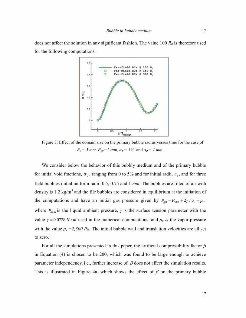
on the dynamics of the primary bubble and on the flow field it generates. Figure 12

28 J. Ma, G.L. Chahine, and C.-T. Hsiao
presents temporal variations of the radius of the primary bubble for different initial void
fractions, . The figure shows the results with the time divided by the bubble period
in the pure liquid to clearly bring out the period shortening with an increase in the void
fraction. The figure also shows that the amplitude of the oscillations of the primary
bubble is noticeably affected by the presence of the surrounding bubbles. This results in
noticeable reduction of the bubble volume oscillations (smaller maximum equivalent
radius and larger minimum equivalent radius) and similarly in measureable reduction of
the bubble period. These reductions have been also observed experimentally
(Jayaprakash et al., 2011). This effect is due to exchange of energy between the primary
bubble and the surrounding bubbles. The energy is absorbed by these surrounding
bubbles and is then released as pressure fluctuations when these bubbles oscillate in turn
in response to the excitation, as seen in Figure 9.
The maximum radius and the period reduction of the primary bubble oscillations are
directly related to the changes in the compressibility of the bubbly mixture surrounding
the bubble due to the presence and behavior of the field bubbles. An indication of this
dependence is the direct link between these changes and the initial void fraction, .
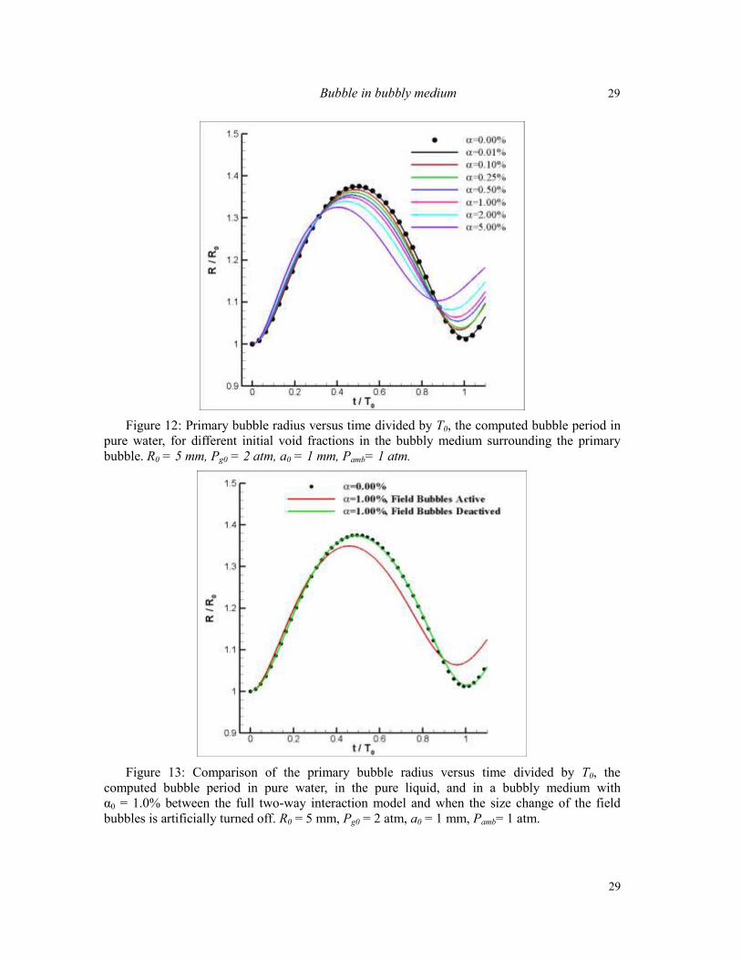
This argument can be further strengthened by considering the results shown in Figure
13. In this figure we compare computations where the full two-way interactions are
considered with the case where, artificially, only field bubble motion is allowed, while
the bubble radius is held constant. Figure 13 shows that the effect of the bubbly medium
on the primary bubble amplitude becomes negligible when the surrounding field
bubbles are prevented from changing size, i.e., when Equations (5) is not solved.
Similarly, a reduction of the period of the primary bubble occurs only when the field
bubbles in the mixture are allowed to change volume in response to the primary bubble
excitation.
0
Bubble in bubbly medium 29
29
Figure 12: Primary bubble radius versus time divided by T0, the computed bubble period in
pure water, for different initial void fractions in the bubbly medium surrounding the primary
bubble. R0 = 5 mm, Pg0 = 2 atm, a0 = 1 mm, Pamb= 1 atm.
Figure 13: Comparison of the primary bubble radius versus time divided by T0, the
computed bubble period in pure water, in the pure liquid, and in a bubbly medium with
α0 = 1.0% between the full two-way interaction model and when the size change of the field
bubbles is artificially turned off. R0 = 5 mm, Pg0 = 2 atm, a0 = 1 mm, Pamb= 1 atm.

30 J. Ma, G.L. Chahine, and C.-T. Hsiao
5.4. Pressure and density variations in the neighborhood of the primary bubble
Figure 14 : Comparison of the pressure at r = 7 mm (r=1.4 R0) under different initial void
fractions.a0 = 1 mm, R0 = 5 mm, Pg0 = 2 atm, Pamb= 1 atm.
As already seen in Figure 11, field bubbles close to the primary bubble respond
strongly to the growth and collapse of the primary bubble. Thus, it is of particular
interest to further examine their effects on the solution by examining the variations of
the pressure and mixture density in the neighborhood of the primary bubble.
Figure 14 shows the pressure time variations at r = 7 mm (1.4 R0) for different
initial void fractions . At this location close to the primary bubble wall, the flow feels
the high pressures generated by the primary bubble very quickly after the bubble wall is
allowed to move. For all cases, the pressure first rises from 1 atm. to a value close to the
pressure inside the primary bubble then starts to decrease until it reaches a minimum,
corresponding to the primary bubble reaching its maximum value. Then, the pressure
gradually increases as the primary bubble collapses following the same pressure versus
time shape as the primary bubble volume versus time. The maximum pressure reached
at the end of the cycle is however smaller than that of the first peak when the primary

Bubble in bubbly medium 31
31
bubble was released because the bubbly mixture attenuates the pressures with the field
bubbles absorbing energy from the main bubble. Figure 14 shows clearly this
attenuation increasing for larger void fractions through an increase in the number
density of field bubbles (since the field radii have been selected to be the same).
Figure 15: Comparison of the time variations of the relative change, 0 0/m m m
of the mixture density at r = 7 mm (r=1.4 R0) under different initial void fractions. a0 = 1mm,
R0 = 5 mm, Pg0 = 2 atm, Pamb= 1 atm.
The corresponding time variations of the mixture densities for various initial void
fractions, are displayed in Figure 15. Here, the temporal variation of the mixture
density, δρ, is defined as the relative local mixture density variation compared to the
initial mixture density, i.e., 0 0/m m m . Since the density is linearly related to
the void fraction through Equation (1), which in turn is determined by the local pressure,
the mixture density oscillates with a period close to that of the primary bubble for all
cases. However, a time delay in the occurrence of the first density peak can be clearly
seen in the figure and increases with the void fraction. This peak density is also shifted

32 J. Ma, G.L. Chahine, and C.-T. Hsiao
relative to the peak in the pressure where the first pressure peak occurs very close to
t = 0 (see Figure 14). This delay, defined as “tshift”, is about 7% of the primary bubble
period for = 0.1% and increases to about 13% for = 2%. This is attributed to the
two-way interactions between the main bubble dynamics and the bubbles in the flow
field. The field bubbles take time to react to the pressure change. This results in finite
time of transfer of the density information between the primary bubble and a field point.
Figure 16 compares the temporal variations of the gas pressure inside a field bubble
located close to the primary bubble and the two-phase field pressure it encounters. The
figure shows that as the primary bubble expands, the pressure around it first rises to a
large value and then decreases in time. As long as this pressure is higher than the sum of
the pressure of the gas inside a field bubble plus the vapor pressure minus the surface
tension, this field bubble continues to lose volume. The gas inside it is compressed until
time tshift, when the inner bubble pressure balances the field pressure. As a result, during
the time [0, tshift], the field bubbles in the considered region get compressed and the
mixture density increases, even while the corresponding field pressure decreases.
Therefore, the p- phase shift can be attributed to the dynamics of the field bubbles in
the two-phase medium, which respond to the field pressure changes slower than the
liquid flow does. The phase shift becomes larger as the void fraction increases and as the
effect of the field bubbles’ dynamics on the primary bubble increases. Further
indications supporting this explanation can be seen in the following section where tshift is
found to become larger as the size of the field bubbles increases and as the natural
period of oscillation of the bubble increases. This finding cannot be captured by
methods assuming homogeneous medium, e.g., (Wardlaw & Luton, 2000, Wardlaw &
Luton, 2003) and the analytical Gilmore equation (Gilmore, 1952). This highlights the
importance of considering the individual bubble dynamics in the dispersed phase for
high fidelity modeling.

Bubble in bubbly medium 33
33
Figure 16: Variations of the gas pressure inside a field bubble and the corresponding
encounter pressure in the two-phase medium for a bubble at a distance of 2.8R0 from the
primary center. 0= 1%. R0 = 5 mm, Pg0 = 2 atm, a0 = 1mm, Pamb= 1 atm.
5.5. Effect of field bubbles size and concentration on primary bubble dynamics
We have illustrated in the previous sections that the dynamics of the primary bubble
is significantly modified by the presence of the dispersed bubbles in the two-phase
medium and have seen that this effect is dependent on the void fraction. To gain further
understanding we consider now the effects of changing the size of the field bubbles. We
consider field bubbles with initial radii between one tenth and one fifth of the radius of
the primary bubble and consider cases with initial void fractions, 0, between 0% and
5%.

34 J. Ma, G.L. Chahine, and C.-T. Hsiao
Figure 17: Primary bubble radius versus time for two initial field bubble radii
(a0=0.5 mm = 0.1R0, and a0=0.75 mm = 0.15R0) and for a set of initial void fractions between 0
and 2%. R0 = 5 mm, Pg0 = 2 atm, Pamb= 1 atm.
Figure 17 compares the variations of the primary bubble radius versus time for
different void fractions and for two initial radii. Overall, as in Figure 12, the results
show that as the void fraction increases, the maximum bubble radius decreases while the
minimum bubble radius increases, i.e. the amplitude of the bubble radius oscillations are
significantly reduced. This is in a good agreement with the solutions of analytical
Gilmore equation. However, the Euler-Lagrange modeling shows less reduction in the
bubble oscillations amplitude than with the Gilmore model and the difference becomes
more and more obvious for increasing 0. This is illustrated in Figure 18a, which shows
the maximum and minimum bubble radii achieved for different void fractions
normalized with the values in pure water. These are shown for three initial bubble
radius values. The figure also shows the results obtained from the Gilmore model. A
significant effect of the void fraction can be seen and differences between the present
results and the homogeneous model are seen to increase with the void fraction. Much
less influence is seen for the initial bubble radius. Under the same initial void fraction,
damping of the oscillations of the primary bubble is a little larger for smaller field
bubbles size. For example, at ~ 1%, the reduction of Rmax is about 2.3% for field

Bubble in bubbly medium 35
35
bubbles of radii r=0.5 mm and 2.1% for a=0.75 mm, but this drops to 1.9% for field
bubbles of radii a=1 mm.
Figure 18: Variation with the void fraction of the maximum and minimum radii, Rmax and
Rmin, relative to the same in the pure liquid for three initial field bubble radii (a0=0.5 mm= 0.1R0,
a0=0.75 mm= 0.15R0, and a0=1.0 mm= R0/5,) and for a set of initial void fractions between 0
and 5%. R0 = 5 mm, Pg0 = 2 atm, Pamb = 1 atm.
The reduction of damping with increasing void fraction relative to the Gilmore
model can be examined by considering the variations in the bubble radius time
dependence as the void fraction is increased. As seen in Figure 19, the bubble at r = 4R0
oscillates at a frequency composed of the primary bubble forcing frequency and its own
natural frequency These oscillations absorb energy from the primary bubble and from
each other, and are responsible for the damping effects onto the primary bubble
dynamics and onto each other. This effect increases as the void fraction increases.
Changes in the void fraction are fed-back to the mixture flow through modification of
the mixture density and sound speed. The modified properties, in turn, affect the
dynamics of the field bubbles by reducing the driving pressure for each bubble. This is

36 J. Ma, G.L. Chahine, and C.-T. Hsiao
reflected in Figure 19, which shows smaller amplitude of the oscillations of the field
bubble size as the void fraction increases, and made further clear in Figure 20, which
compares the amplitudes of the secondary oscillation for the different initial void
fractions. This effect is actually self-limiting. As the void fraction increases, less energy
is transmitted to the field bubbles and they in turn have less chance to absorb the energy.
The above discussion can be helped by also comparing in Figure 19 the above discussed
field bubble oscillations with those obtained when imposing only one-way coupling
(i.e., the mixture flow does not see the presence of the field bubbles and has the same
properties as a pure liquid). In this case the field bubbles size oscillates with a much
larger amplitude than when the correct two-way coupling is applied. Obviously, in the
Gilmore solution, these damping effects happening between the field bubbles due to
their own interaction are not included, thus resulting in over predicted energy reduction
effects on the primary bubble dynamics.
Figure 19: (Left) Comparison of the radius versus time of a field bubble initially at r = 4R0
for different initial void fractions in the mixture. Note the reduction in response as the void
fraction increases. a0 = 1 mm, R0 = 5 mm, Pg0 = 2 atm, Pamb= 1 atm. (Right) Filtered radius
variation, a’ versus time for the same bubbles in left, where a
’ is the amplitude of the secondary
bubble oscillations under their own natural frequency.

Bubble in bubbly medium 37
37
Figure 20: Effect of the void fraction on the amplitude of the secondary oscillations at the
field bubble resonance frequency, a’, shown in above right plot of Figure 19.
Similarly, the trend of reduced damping when increasing the size of the field bubbles
can be explained by considering the field bubble radius oscillations in Figure 21. A field
bubble of different sizes located at r = 4R0 is considered for the same = 1.0%.
Though overall, the bubble sizes oscillate with similar trends, by increasing the size of
the field bubbles we bring their natural frequency of oscillations closer to that of the
primary bubble and the frequency of the secondary oscillations is reduced. This results
in less energy dissipation and weaker local pressure perturbations than with the high
frequency oscillations of the smaller field bubbles. As a result, as shown in Figure 22
with a same initial void fraction , the attenuation of pressure becomes slightly weaker
as the size of the field bubbles increases.
Figure 23 shows the effect of the presence of the field bubbles on the period of the
primary bubble. The results are normalized by the bubble period in a pure liquid (i.e. at
= 0) to illustrate the reduction in the period when in a two-phase medium. The period
reduction effect is seen to increase with the void fraction and to not depend much on the
field bubbles size. This numerically computed effect is much larger than that estimated

38 J. Ma, G.L. Chahine, and C.-T. Hsiao
using the Gilmore equation and other analytical expressions assuming homogenous
flows. For example, if we consider that the period reduction is only due to a reduction in
the mixture density, the Rayleigh time would be modified as
0
0, 0
0
(1 )2 .
lRayleigh
g amb
T RP P (22)
Accordingly a bubbly mixture with = 5% would result in about 2.2% reduction in the
period; however, it is around 13% in Figure 23. This significant difference should be
attributed to the interactive dynamics between the field bubbles and the effect of their
response on the primary bubble dynamics, which are accounted for in the present
simulations.
Figure 21: Comparison of the radius versus time of a field bubble initially at r = 4R0 for
different initial bubble sizes. = 1.0%, R0 = 5 mm, Pg0 = 2 atm, Pamb= 1 atm.

Bubble in bubbly medium 39
39
Figure 22: Comparison of the pressure at r = 7 mm with different initial field bubble sizes.
= 1.0%, R0 = 5 mm, Pg0 = 2 atm, Pamb= 1 atm.
Figure 23: Comparison of the bubble period achieved by the primary bubble for three initial
field bubble radii (a0=0.5 mm= 0.1R0, 0.75 mm= 0.15R0, and 1.0 mm= R0/5,) and for a set of
initial void fractions between 0 and 5%. R0 = 5 mm, Pg0 = 2 atm, a0 = 0.5~1 mm, Pamb= 1 atm.

40 J. Ma, G.L. Chahine, and C.-T. Hsiao
5.6. Effect of field bubbles size and concentration on Phase shift
Here we consider the effect of the field bubbles on the normalized mixture density
change 0 0/m m m and on the pressure distribution. Figure 24 displays the
curves of mixture density versus time monitored at a point in the near field of the
primary bubble (r=7 mm=1.4R0) under the different conditions used above. Overall, all
cases show that as the void fraction increases the phase shift becomes more and more
significant due to the increased effect of the field bubbles on the primary bubble.
However, this effect depends on both the bubble sizes and the void fraction. Figure 25
quantitatively compares tshift for the different conditions to illustrate this effect. The
Gilmore equation does not capture tshift due to the homogenous medium assumptions
where the mixture density is only a function of the pressure without consideration to
bubble dynamics in the field. We can see in the figure that for a given initial bubble size,
tshift becomes larger as the void fraction increases. However, the effect of the field
bubbles sizes for the same is more complex. As seen in Figure 25, a switch in
behavior occurs as the void fraction increases. At small void fractions, tshift becomes
larger as the initial bubble radius increases. This is due to the fact that the natural
bubble period increases with the size. Therefore, these bubbles take a longer time to
reach balance with the flow. This is also clearly seen in the bubble size variation history
curves plotted in Figure 21, where we see an initial stage of bubble size decrease
(mixture density increasing) while the pressure is also dropping. The duration of this
stage is longer for the larger bubbles. However, this trend reverts for the higher void
fraction, here for . This can be explained by the same reasoning given
previously about increased damping and reduced secondary oscillations of the field
bubble at their own natural frequency as the void fraction increases.
0 2%

Bubble in bubbly medium 41
41
Figure 24: Variation of the relative change of the mixture density, δρ = (ρm - ρm0 )/ ρm0, at a
radial distance of r = 7 mm for two initial field bubble radii (a0=0.5 mm= 0.1R0, and a0=0.75
mm= 0.15R0) and for a set of initial void fractions between 0 and 5%. R0 = 5 mm, Pg0 = 2 atm,
a0 = 0.5~1 mm, Pamb= 1 atm. (Refer to above Figure 15 for comparison with cases of a0=1.0
mm= R0/5)
Figure 25: Comparison of the phase shift between pressure and density, tshift , for three initial
field bubble radii (a0=0.5 mm = 0.1R0, a0 = 0.75 mm = 0.15R0 , and a0 =1.0 mm = R0/5) and for
a set of initial void fractions between 0 and 5%. R0 = 5 mm, Pg0 = 2 atm, a0 = 0.5~1 mm, Pamb=
1 atm.

42 J. Ma, G.L. Chahine, and C.-T. Hsiao
6. CONCLUSIONS
The dynamics of a primary bubble oscillating in a bubbly flow is studied using a 3D
two-way coupled Euler-Lagrange model, which treats the two-phase medium as a
continuum while the field bubbles are tracked in a Lagrangian fashion. The two-phase
medium conditions were varied by changing the size and number of the field bubbles in
the two-phase medium. This modified also the initial void fractions.
The study has shown that bubbly dynamics is modified as follows in a bubbly
medium. The surrounding bubbly medium absorbs the energy emitted from the primary
bubble thereby damping the bubble oscillations and resulting in noticeable reductions in
both the maximum achieved primary bubble radius and bubble period. These effects
become more significant when the void fraction of the mixture increases.
Under the same void fraction, smaller size field bubbles in the two-phase medium
(or alternatively larger ratio of primary bubble to surrounding bubbles) result in stronger
damping effects in terms of achieved maximum radius of the primary bubble. However,
varying the field bubble size (or alternatively changing the ratio of primary bubble to
surrounding bubbles) does not seem to have a noticeable effect on the primary bubble
period. This implies that for developing a correction term for the homogeneous model,
it will be possible to correct the bubble period based on the mixture void fraction.
However, more work is needed to correct the amplitude as there is a need to study this
further for cases where the primary bubble becomes in the same range and even smaller
than the surrounding field bubbles.
On the other hand, the dynamics of the field bubbles result in a phase-shift between
the density and the pressure time variations in the two-phase medium and this is
strongly influenced by the bubble sizes and the void fraction. The effects cannot be
captured by analytical solutions treating the mixture as a homogeneous medium. The
phase shift increases with the void fraction but is a more complex function of the size of
the dispersed small bubbles. At smaller void fractions larger bubbles produce larger
phase shifts but this trend is revered at the higher void fractions. Here again, for future
development of corrections for the homogeneous model, more work is needed to

Bubble in bubbly medium 43
43
address cases where the primary bubble becomes in the same range and even smaller
than the surrounding field bubbles. Also, investigating how the pressure ratio between
the initial pressures inside the primary and field bubbles affects the differences between
the homogeneous models and the present model will provide insight to the development
of a correction strategy.
7. ACKNOWLEDGMENTS
This work was supported by the Department of Energy under contract DE-FG02-
07ER84839. This work was also supported in part by grants of computer time from The
National Energy Research Scientific Computing Center (NERSC), a scientific
computing facility for the Office of Science in the U.S. Department of Energy.
8. NOMENCLATURE
DC Drag coefficient
LC Lift coefficient
Interface curvature
rF Froude number
P Pressure at bubble wall
ambP Ambient Pressure
P Pressure at infinity
r Radial location
a0 Initial bubble size in bubbly medium
R Primary bubble radius
Rmax Maximum radius of primary bubble
eR Reynolds number
U, V, W Contravariant velocity components
eW b Weber number
c Sound speed in the bubbly medium
c Reference sound speed
g Acceleration of gravity vector
k Polytropic gas constant
p Pressure
C

44 J. Ma, G.L. Chahine, and C.-T. Hsiao
vp Vapor pressure
t Time
shiftt Phase shift between the mixture density and pressure variations
T0 Duration of the first cycle of oscillations of the primary bubble
u Velocity
charcu Characteristic velocity
V Volume
Void fraction
c Artificial compressibility factor
Surface tension at air-water interface ω Vorticity
m Density of the mixture
δρ Variation of mixture density
Reference density
Dynamic Viscosity
Kinematic Viscosity
Pseudo-time
, , Curvilinear coordinates
Subscripts 0 Initial condition
,b bubble Bubble property
enc Encountered by the bubble
, ,i j k Indices
g Gas property
l Liquid property
m Mixture property
9. REFERENCES
AANJANEYA, M., PATKAR, S. & FEDKIW, R. 2013. A monolithic mass tracking
formulation for bubbles in incompressible flow. Journal of Computational
Physics, 247, 17-61.
ALIABADI, A. & TAKLIFI, A. 2012. The effect of magnetic field on dynamics of gas
bubbles in visco-elastic fluids. Applied Mathematical Modelling, 36, 2567-2577.
ANDERSON, W. K., THOMAS, J. L. & VAN LEER, B. 1986. Comparison of finite volume
flux vector splittings for the Euler equations. AIAA journal, 24, 1453-1460.

Bubble in bubbly medium 45
45
ARIENTI, M. & SUSSMAN, M. 2014. An embedded level set method for sharp-interface
multiphase simulations of Diesel injectors. International Journal of Multiphase
Flow, 59, 1-14.
ARNDT, R. E. A. 1981. Cavitation in fluid machinery and hydraulic structures. Annual
Review of Fluid Mechanics, 13, 273-328.
BALACHANDAR, S. & EATON, J. K. 2010. Turbulent dispersed multiphase flow. Annual
Review of Fluid Mechanics, 42, 111-133.
BATCHELOR, G. K. 1967. An introduction to fluid dynamics, Cambridge university press.
BESANT, W. 1859. Hydrostatics and hydrodynamics. Cambridge University Press,
London, Art, 158, 1859.
BJERKNES, V. F. K. 1906. Fields of Force, New York, Columbia University Press.
BLAKE, J. R. & GIBSON, D. C. 1987. Cavitation bubbles near boundaries. Annual Review
of Fluid Mechanics, 19, 99-123.
BRENNEN, C. E. 1995. Cavitation and bubble dynamics, Oxford University Press
BRENNEN, C. E., 2005, Fundamentals of Multiphase Flows, Cambridge University
Press.
CALVISI, M. L., LINDAU, O., BLAKE, J. R. & SZERI, A. J. 2007. Shape stability and
violent collapse of microbubbles in acoustic traveling waves. Physics of Fluids,
19, 047101.
CAPECELATRO, J. & DESJARDINS, O. 2013. An Euler–Lagrange strategy for simulating
particle-laden flows. Journal of Computational Physics, 238, 1-31.
CAPRETTO, L., CHENG, W., HILL, M. & ZHANG, X. L. 2011. Micromixing Within
Microfluidic Devices. Microfluidics: Technologies and Applications, 304, 27-68.
CHAHINE, G. L., 1983, Cloud Cavitation: Theory. Proc. 14th Symposium on Naval
Hydrodynamics, Ann Arbor, Michigan, National Academy Press, pp. 165-194.
CHAHINE, G. L. and DURAISWAMI, R., 1992, Dynamical Interaction in a multi-Bubble
Cloud. ASME J. Fluids Eng., 114(4), pp. 680-686.
CHAHINE, G., DURAISWAMI, R. & KALUMUCK, K. 1996. Boundary element method for
calculating 2-D and 3-D underwater explosion bubble loading on nearby
structures including fluid structure interaction effects. Naval Surface Weapons
Center, Dahlgren Division, Weapons Research and Technology Department,
Technical Report NSWCDD/TR-93/46.
CHAHINE, G. & KALUMUCK, K. 1998. BEM software for free surface flow simulation
including fluid-structure interaction effects. International Journal of Computer
Applications in Technology, 11, 177-198.
CHAHINE, G. L. 2009. Numerical simulation of bubble flow interactions. Journal of
Hydrodynamics, Ser. B, 21, 316-332. CHAHINE, G. L., HSIAO, C.-T., CHOI, J.-K., AND WU, X., 2008, Bubble Augmented Waterjet
Propulsion: Two-Phase Model Development and Experimental Validation, 27th
Symposium on Naval Hydrodynamics, Seoul, Korea, 5-10, October 2008.
CHAHINE, G. L. & HARRIS, G. 1997. Development and validation of a multicycle bubble
model for UNDEX application. 68th Shock and Vibration Symposium. Hunt
Valley, MD.

46 J. Ma, G.L. Chahine, and C.-T. Hsiao
CHAHINE, G. L. & HSIAO, C.-T. Modeling 3D unsteady sheet cavities using a coupled
UnRANS-BEM code. In: Proc. 23rd ONR Symposium on Naval
Hydrodynamics, 2000.
CHAHINE, G. L. & HSIAO, C.-T. 2012. Modeling microbubble dynamics in biomedical
applications. Journal of Hydrodynamics, Ser. B, 24, 169-183.
CHAHINE, G. L. & LIU, H. L. 1985. A singular-perturbation theory of the growth of a
bubble cluster in a superheated liquid. Journal of Fluid Mechanics, 156, 257-
279.
CHEN, J., YANG, N., GE, W. & LI, J. 2009. Computational fluid dynamics simulation of
regime transition in bubble columns incorporating the dual-bubble-size model.
Industrial & Engineering Chemistry Research, 48, 8172-8179.
CHOI, J., HSIAO, C.-T., CHAHINE, G. & CECCIO, S. 2009. Growth, oscillation and
collapse of vortex cavitation bubbles. Journal of Fluid Mechanics, 624, 255.
CHORIN, A. J. 1967. A numerical method for solving incompressible viscous flow
problems. Journal of computational physics, 2, 12-26.
CHUNG, S. K. & CHO, S. K. 2009. 3-D manipulation of millimeter- and micro-sized
objects using an acoustically excited oscillating bubble. Microfluidics and
Nanofluidics, 6, 261-265.
COLEMAN, A. J., SAUNDERS, J. E., CRUM, L. A. & DYSON, M. 1987. Acoustic Cavitation
Generated by an Extracorporeal Shockwave Lithotripter. Ultrasound in Medicine
and Biology, 13, 69-76.
COMMANDER, K. W. & PROSPERETTI, A. 1989. Linear pressure waves in bubbly liquids:
Comparison between theory and experiments. The Journal of the Acoustical
Society of America, 85, 732.
DARMANA, D., DEEN, N. & KUIPERS, J. 2006. Parallelization of an Euler–Lagrange
model using mixed domain decomposition and a mirror domain technique:
Application to dispersed gas–liquid two-phase flow. Journal of computational
physics, 220, 216-248.
DARMANA, D., HENKET, R., DEEN, N. & KUIPERS, J. 2007. Detailed modelling of
hydrodynamics, mass transfer and chemical reactions in a bubble column using a
discrete bubble model: Chemisorption of CO2 into NaOH solution, numerical
and experimental study. Chemical Engineering Science, 62, 2556-2575.
DE GRAAF, K., PENESIS, I. & BRANDNER, P. Comparison of the Rayleigh–Plesset and
Gilmore Equations and Additional Aspects for the Modelling of Seismic Airgun
Bubble Dynamics. In: 18th Australasian Fluid Mechanics Conference, 2012. 1-
4.
FERRANTE, A., AND ELGHOBASHI, S., 2004, On the physical mechanisms of drag
reduction in a spatially developing turbulent boundary layer laden with
microbubbles, J. of Fluid Mechanics, 503, pp. 345-355.
FRANCOIS, M. M., CUMMINS, S. J., DENDY, E. D., KOTHE, D. B., SICILIAN, J. M. &
WILLIAMS, M. W. 2006. A balanced-force algorithm for continuous and sharp
interfacial surface tension models within a volume tracking framework. Journal
of Computational Physics, 213, 141-173.

Bubble in bubbly medium 47
47
FUSTER, D. & COLONIUS, T. 2011. Modelling bubble clusters in compressible liquids.
Journal of Fluid Mechanics, 688, 352-389.
GEERS, T. L. & HUNTER, K. S. 2002. An integrated wave-effects model for an
underwater explosion bubble. The Journal of the Acoustical Society of America,
111, 1584.
GILMORE, F. 1952. The collapse and growth of a spherical bubble in a viscous
compressible liquid. Hydrodynamics Lab Report No. 26-4. Pasadena, CA.:
Califonia Institute of Technology.
GUILLEN, D. P., GRIMMETT, T., GANDRIK, A. M. & ANTAL, S. P. 2011. Development of a
computational multiphase flow model for Fischer Tropsch synthesis in a slurry
bubble column reactor. Chemical Engineering Journal, 176, 83-94.
HABERMAN, W. & MORTON, R. 1953. An experimental investigation of the drag and
shape of air bubbles rising in various liquids. DTIC Document.
HERRING, C. 1941. Theory of the pulsations of the gas bubble produced by an
underwater explosion, Columbia Univ., Division of National Defense Research.
HILGENFELDT, S., BRENNER, M. P., GROSSMANN, S. & LOHSE, D. 1998. Analysis of
Rayleigh-Plesset dynamics for sonoluminescing bubbles. Journal of Fluid
Mechanics, 365, 171-204.
HODGES, B., STREET, R. & ZANG, Y. A method for simulation of viscous, nonlinear,
free-surface flows. In: 20th Symposium on Naval Hydrodynamics, 1996. 791-
809. HSIAO, C.-T. , 1996, “Numerical study of the Tip Vortex Flow over a Finite-Span
Hydrofoil,” Ph.D. Thesis, Department of Mechanical Engineering, The
Pennsylvania State University.
HSIAO, C.-T. & CHAHINE, G. 2008. Numerical study of cavitation inception due to
vortex/vortex interaction in a ducted propulsor. Journal of Ship Research, 52,
114-123.
HSIAO, C.-T. & CHAHINE, G. L. 2012. Effect of a propeller and gas diffusion on bubble
nuclei distribution in a liquid. Journal of Hydrodynamics, Ser. B, 24, 809-822.
HSIAO, C.-T., CHAHINE, G. L. & LIU, H.-L. 2003. Scaling effect on prediction of
cavitation inception in a line vortex flow. Journal of fluids engineering, 125, 53-
60.
HSIAO, C.-T., CHOI, J.-K., SINGH, S., CHAHINE, G., HAY, T., ILINSKII, Y. A.,
ZABOLOTSKAYA, E., HAMILTON, M., SANKIN, G. & YUAN, F. 2013a. Modelling
single-and tandem-bubble dynamics between two parallel plates for biomedical
applications. Journal of Fluid Mechanics, 716, 137-170.
HSIAO, C.-T., LU, X. & CHAHINE, G. 2010. Three-dimensional modeling of the
dynamics of therapeutic ultrasound contrast agents. Ultrasound in medicine &
biology, 36, 2065-2079.
HSIAO, C.-T. & PAULEY, L. L. 1998. Numerical study of the steady-state tip vortex flow
over a finite-span hydrofoil. Journal of fluids engineering, 120, 345-353.

48 J. Ma, G.L. Chahine, and C.-T. Hsiao
HSIAO, C. & CHAHINE, G. 2001. Numerical Simulation of Bubble Dynamics in a Vortex
Flow Using Moving Chimera Grid and Navier-Stokes Computations. CAV2001,
Pasadena, CA.
HSIAO, C. T., WU, X., MA, J. & CHAHINE, G. L. 2013b. Numerical and experimental
study of bubble entrainment due to a horizontal plunging jet. International
Shipbuilding Progress, 60, 435-469.
JAYAPRAKASH, A., SINGH, S. & CHAHINE, G. 2011. Experimental and Numerical
Investigation of Single Bubble Dynamics in a Two-Phase Bubbly Medium.
Transactions of the ASME-I-Journal of Fluids Engineering, 133, 121305.
JOHNSON, J. V. E., CHAHINE, G. L., LINDENMUTH, W. T., CONN, A. F., FREDERICK, G. S.
& GIACCHINO, J. G. J. 1982. Cavitating and Structered Jets for Mechanical Bits
to Increase Drilling Rate. The ASME Publication, 82-Pet-13, 1-16.
JOHNSON, V. & HSIEH, T. The influence of the trajectories of gas nuclei on cavitation
inception. In: Sixth Symposium on Naval Hydrodynamics, 1966. 163-179.
KALUMUCK, K., CHAHINE, G., HSIAO, C. & CHOI, J. Remediation and disinfection of
water using jet generated cavitation. In: 5th International Symposium on
Cavitation (CAV 2003), Osaka, Japan, 2003.
KALUMUCK, K. M. & CHAHINE, G. L. 2000. The use of cavitating jets to oxidize organic
compounds in water. Journal of Fluids Engineering-Transactions of the Asme,
122, 465-470.
KELLER, J. B. & KOLODNER, I. I. 1956. Damping of underwater explosion bubble
oscillations. Journal of Applied Physics, 27, 1152-1161.
KELLER, J. B. & MIKSIS, M. 1980. Bubble oscillations of large amplitude. The Journal of
the Acoustical Society of America, 68, 628.
KENNEDY, J. E. 2005. High-intensity focused ultrasound in the treatment of solid
tumours. Nat Rev Cancer, 5, 321-7.
KITAGAWA, A., MURAI, Y. & YAMAMOTO, F. 2001. Two-way coupling of Eulerian–
Lagrangian model for dispersed multiphase flows using filtering functions.
International journal of multiphase flow, 27, 2129-2153.
KRIEGER, J. R. & CHAHINE, G. L. 2005. Acoustic signals of underwater explosions near
surfaces. The Journal of the Acoustical Society of America, 118, 2961.
LAUER, E., HU, X., HICKEL, S. & ADAMS, N. 2012. Numerical modelling and
investigation of symmetric and asymmetric cavitation bubble dynamics.
Computers & Fluids, 69, 1-19.
LAW, D., BATTAGLIA, F. & HEINDEL, T. J. Stability issues for gas-liquid flows in bubble
columns. In: ASME 2007 International Mechanical Engineering Congress and
Exposition, 2007. American Society of Mechanical Engineers, 53-61.
LAW, D., BATTAGLIA, F. & HEINDEL, T. J. 2008. Model validation for low and high
superficial gas velocity bubble column flows. Chemical Engineering Science,
63, 4605-4616.
LAW, D., JONES, S. T., HEINDEL, T. J. & BATTAGLIA, F. 2011. A Combined Numerical
and Experimental Study of Hydrodynamics for an Air-Water External Loop
Airlift Reactor. Journal of fluids engineering, 133, 021301.

Bubble in bubbly medium 49
49
LORAINE, G., CHAHINE, G., HSIAO, C.-T., CHOI, J.-K. & ALEY, P. 2012. Disinfection of
gram-negative and gram-positive bacteria using DynaJets® hydrodynamic
cavitating jets. Ultrasonics sonochemistry, 19, 710-717.
MA, J., HSIAO, C.-T. AND CHAHINE, G.L., 2015. Euler-Lagrange Simulations of Bubble
Cloud Dynamics near a Wall, ASME J. Fluids Eng., 137(4), pp. 041301-10
MADADI-KANDJANI, E. & XIONG, Q. 2014. Validity of the spring-backed membrane
model for bubble–wall interactions with compliant walls. Computers & Fluids,
96, 116-121.
MIKSIS, M. J. & TING, L. 1984. Nonlinear radial oscillations of a gas bubble including
thermal effects. The Journal of the Acoustical Society of America, 76, 897.
MITRAGOTRI, S. 2005. Innovation - Healing sound: the use of ultrasound in drug
delivery and other therapeutic applications. Nature Reviews Drug Discovery, 4,
255-260.
MOHOLKAR, V., SENTHIL KUMAR, P. & PANDIT, A. 1999. Hydrodynamic cavitation for
sonochemical effects. Ultrasonics Sonochemistry, 6, 53-65.
MORCH, K.A., 1981, Cavity cluster dynamics and cavitation erosion. Proc. ASME.
Cavitation and Polyphase Flow Forum, pp. 1-10.
OH, J. M., KIM, P. & KANG, I. S. 2001. Chaotic oscillation of a bubble in a weakly
viscous dielectric fluid under electric fields. Physics of Fluids, 13, 2820.
OHL, C. D., ARORA, M., DIJKINK, R., JANVE, V. & LOHSE, D. 2006. Surface cleaning
from laser-induced cavitation bubbles. Applied Physics Letters, 89.
PLESSET, M. 1949. The dynamics of cavitation bubbles. J. appl. Mech, 16, 227-282.
PLESSET, M. S. & PROSPERETTI, A. 1977. Bubble dynamics and cavitation. Annual
Review of Fluid Mechanics, 9, 145-185.
PROSPERETTI, A. 1982. A generalization of the Rayleigh–Plesset equation of bubble
dynamics. Physics of Fluids (1958-1988), 25, 409-410.
PROSPERETTI, A. 1987. The equation of bubble dynamics in a compressible liquid.
Physics of Fluids, 30, 3626.
PROSPERETTI, A. 1991. The thermal behaviour of oscillating gas bubbles. Journal of
Fluid Mechanics, 222, 587-616.
PROSPERETTI, A., CRUM, L. A. & COMMANDER, K. W. 1988. Nonlinear bubble
dynamics. The Journal of the Acoustical Society of America, 83, 502.
PROSPERETTI, A. & HAO, Y. 1999. Modelling of spherical gas bubble oscillations and
sonoluminescence. Philosophical Transactions of the Royal Society of London.
Series A: Mathematical, Physical and Engineering Sciences, 357, 203-223.
PROSPERETTI, A. & LEZZI, A. 1986. Bubble dynamics in a compressible liquid. Part 1.
First-order theory. J. FLUID MECH., 1986, 168, 457-478.
RAJU, R., SINGH, S., HSIAO, C.-T. & CHAHINE, G. 2011. Study of Pressure Wave
Propagation in a Two-Phase Bubbly Mixture. Transactions of the ASME-I-
Journal of Fluids Engineering, 133, 121302.
RAYLEIGH, L. 1917. VIII. On the pressure developed in a liquid during the collapse of a
spherical cavity. The London, Edinburgh, and Dublin Philosophical Magazine
and Journal of Science, 34, 94-98.

50 J. Ma, G.L. Chahine, and C.-T. Hsiao
ROE, P. L. 1981. Approximate Riemann solvers, parameter vectors, and difference
schemes. Journal of computational physics, 43, 357-372.
SEO, J. H., LELE, S. K. & TRYGGVASON, G. 2010. Investigation and modeling of bubble-
bubble interaction effect in homogeneous bubbly flows. Physics of Fluids, 22,
063302.
SHAMS, E., FINN, J. & APTE, S. 2011. A numerical scheme for Euler–Lagrange
simulation of bubbly flows in complex systems. International Journal for
Numerical Methods in Fluids, 67, 1865-1898.
SINGH, R. & SHARMA, S. 2012. Development of suitable photobioreactor for algae
production–A review. Renewable and Sustainable Energy Reviews, 16, 2347-
2353.
SPELT, P. & BIESHEUVEL, A. 1997. On the motion of gas bubbles in homogeneous
isotropic turbulence. Journal of Fluid Mechanics, 336, 221-244.
SPELT, P. & MATAR, O. 2006. Collapse of a bubble in an electric field. Physical Review
E, 74, 046309.
SUSSMAN, M. 2003. A second order coupled level set and volume-of-fluid method for
computing growth and collapse of vapor bubbles. Journal of Computational
Physics, 187, 110-136. VAN LEER, B., THOMAS, J.L., ROE, P.L. AND NEWSOME, R.W., 1987, “A Comparison of
Numerical Flux Formulas for the Euler and Navier-Stokes Equation,” AIAA Paper
No. 87-1104-CP.
VAN SINT ANNALAND, M., DEEN, N. & KUIPERS, J. 2005. Numerical simulation of gas–
liquid–solid flows using a combined front tracking and discrete particle method.
Chemical Engineering Science, 60, 6188-6198.VAN WIJNGAARDEN, L., 1964. On
the Collective Collapse of a Large Number of Gas Bubbles in Water”,
Proceedings 11th International Congress of Applied Mechanics, Springer,
Berlin, pp.854-861.
VAN WIJNGAARDEN, L., 1968, On the Equations of Motion for mixtures of Liquid and
Gas Bubbles, J. Fluid Mech. 33(3), pp.465-474
VAN WIJNGAARDEN, L., 1972, One-Dimensional Flow of Liquids Containing Small Gas
Bubbles. Annual Review of Fluid Mechanics. 4, pp.369-396
WANG, Q. & BLAKE, J. 2010. Non-spherical bubble dynamics in a compressible liquid.
Part 1. Travelling acoustic wave. Journal of Fluid Mechanics, 659, 191-224.
WARDLAW, A. & LUTON, J. Fluid-structure coupling methodology for undersea
weapons. In: 2 nd International Conference on Fluid Structure Interaction, 2003.
251-261.
WARDLAW, J., ANDREW B & LUTON, J. A. 2000. Fluid-structure interaction mechanisms
for close-in explosions. Shock and Vibration, 7, 265-275.
WARDLAW, J., ANDREW B & MAIR, H. U. 1998. Spherical solutions of an underwater
explosion bubble. Shock and Vibration, 5, 89-102.
WU, X., CHOI, J.-K., HSIAO, C.-T. & CHAHINE, G. L. Bubble augmented waterjet
propulsion: Numerical and experimental studies. In: Proc. 28th Symposium on
Naval Hydrodynamics, 2010.

Bubble in bubbly medium 51
51
WU, X., CHOI, J.-K., SINGH, S., HSIAO, C-T, AND CHAHINE, G. L. , 2012. Experimental
and Numerical Investigation of Bubble Augmented Waterjet Propulsion. J. of
Hydrodynamics, 24(5), pp.635-647.
WU, Y. & GIDASPOW, D. 2000. Hydrodynamic simulation of methanol synthesis in gas–
liquid slurry bubble column reactors. Chemical Engineering Science, 55, 573-
587.
XIANG, M., CHEUNG, S., YEOH, G., ZHANG, W. & TU, J. 2011. On the numerical study of
bubbly flow created by ventilated cavity in vertical pipe. International Journal
of Multiphase Flow, 37, 756-768.
XIANG, M., JIANG, Z., ZHANG, W. & TU, J. 2014. Numerical Modeling and Analysis of
Gas Entrainment for the Ventilated Cavity in Vertical Pipe. Chinese Journal of
Chemical Engineering, 22, 252-260.
YASUI, K. 1999. Effect of a magnetic field on sonoluminescence. Physical Review E, 60,
1759.
YUAN, F., SANKIN, G. & ZHONG, P. 2011. Dynamics of tandem bubble interaction in a
microfluidic channel. The Journal of the Acoustical Society of America, 130,
3339-3346.
ZHANG, S., DUNCAN, J. H. & CHAHINE, G. L. 1993. The final stage of the collapse of a
cavitation bubble near a rigid wall. Journal of Fluid Mechanics, 257, 147-181.
ZHONG, P., ZHOU, Y. & ZHU, S. 2001. Dynamics of bubble oscillation in constrained
media and mechanisms of vessel rupture in SWL. Ultrasound in medicine &
biology, 27, 119-134.