speed prediction for two-lane rural highways · nelson irizarry, kelly d. parma, karin m. bauer,...
TRANSCRIPT

Speed Prediction for Two-LaneRural HighwaysPUBLICATION NO. 99-171 AUGUST 2000
Research, Development, and TechnologyTurner-Fairbank Highway Research Center6300 Georgetown PikeMcLean, VA 22101-2296


Technical Report Documentation Page
1. Report No.FHWA-RD-99-171
2. Government Accession No. 3. Recipient's Catalog No.
4. Title and SubtitleSPEED PREDICTION FOR TWO-LANE RURAL HIGHWAYS
5. Report Date
6. Performing Organization Code
7. Author(s)Kay Fitzpatrick, Lily Elefteriadou, Douglas W. Harwood, Jon M.Collins, John McFadden, Ingrid B. Anderson, Raymond A. Krammes,Nelson Irizarry, Kelly D. Parma, Karin M. Bauer, and Karl Passetti
8. Performing Organization Report No.
9. Performing Organization Name and AddressTexas Transportation InstituteThe Texas A&M University SystemCollege Station, Texas 77843-3135
10. Work Unit No. (TRAIS)
11. Contract or Grant No.DTFH61-95-R-00084
12. Sponsoring Agency Name and Address
Office of Safety Research and DevelopmentFederal Highway Administration6300 Georgetown PikeMcLean, Virginia 22101-2296
13. Type of Report and Period Covered
Final ReportSeptember 1995 - June 1999
14. Sponsoring Agency Code
15. Supplementary NotesContracting Officer’s Technical Representative (COTR): Ann Do, HRDS; [email protected]
16. AbstractDesign consistency refers to the conformance of a highway’s geometry to driver expectancy. Drivers make fewer errorsin the vicinity of geometric features that conform to their expectations. A technique to evaluate the consistency of adesign is to evaluate changes in operating speeds along an alignment. To use operating speed as a consistency toolrequires the ability to accurately predict speeds as a function of the roadway geometry. In this research project, severalefforts were undertaken to predict operating speed for different conditions such as on horizontal, vertical, and combinedcurves; on tangent sections using alignment indices; on grades using the TWOPAS model; and prior to or after ahorizontal curve. The findings from the different efforts were incorporated into a speed-profile model. The model canbe used to evaluate the design consistency of the roadway or can be used to develop a speed profile for an alignment.The model considers both horizontal and vertical curvature and the acceleration or deceleration behavior as a vehiclemoves from one feature to another.
17. Key Words
Two-lane rural highway, speed-prediction equations,acceleration/deceleration, IHSDM.
18. Distribution Statement
This document is available to the public via internet accessat www.tfhrc.gov/safety/ihsdm/ihsdm.htm
19. Security Classif. (of this report)Unclassified
20. Security Classif. (of this page)Unclassified
21. No. of Pages217
22. Price
Form DOT F 1700.7 (8-72)

TABLE OF CONTENTS
1. INTRODUCTION . . . . . . . . . . . . . . . . . . . . . . . . . . . . . . . . . . . . . . . . . . . . . . . . . . . . . . . . . .BACKGROUND . . . . . . . . . . . . . . . . . . . . . . . . . . . . . . . . . . . . . . . . . . . . . . . . . . . . . . . . .OBJECTIVES . . . . . . . . . . . . . . . . . . . . . . . . . . . . . . . . . . . . . . . . . . . . . . . . . . . . . . . . . . . .ORGANIZATION OF THE REPORT . . . . . . . . . . . . . . . . . . . . . . . . . . . . . . . . . . . . . . . . .
2. PREVIOUS WORK ON PREDICTING SPEEDS ON TWO-LANERURAL HIGHWAYS . . . . . . . . . . . . . . . . . . . . . . . . . . . . . . . . . . . . . . . . . . . . . . . . . . . . . . . .
EVALUATION OF DESIGN CONSISTENCY . . . . . . . . . . . . . . . . . . . . . . . . . . . . . . . . . .ESTIMATION OF OPERATING SPEED . . . . . . . . . . . . . . . . . . . . . . . . . . . . . . . . . . . . . .SUMMARY OF LITERATURE REVIEW . . . . . . . . . . . . . . . . . . . . . . . . . . . . . . . . . . . . . .
3. PREDICTING SPEEDS ON TWO-LANE RURAL HIGHWAY CURVES . . . . . . . . . . . .DATA COLLECTION METHODOLOGY . . . . . . . . . . . . . . . . . . . . . . . . . . . . . . . . . . . . .SPEED-PREDICTION EQUATIONS FOR PASSENGER CARS ON
HORIZONTAL AND VERTICAL CURVES . . . . . . . . . . . . . . . . . . . . . . . . . . . . . . . . .PRELIMINARY MODEL DEVELOPMENT . . . . . . . . . . . . . . . . . . . . . . . . . . . . . . . . . . . .EVALUATION OF SPIRAL TRANSITIONS . . . . . . . . . . . . . . . . . . . . . . . . . . . . . . . . . . .OTHER VEHICLE TYPES . . . . . . . . . . . . . . . . . . . . . . . . . . . . . . . . . . . . . . . . . . . . . . . . . .SUMMARY . . . . . . . . . . . . . . . . . . . . . . . . . . . . . . . . . . . . . . . . . . . . . . . . . . . . . . . . . . . . .
4. PREDICTING SPEEDS ON TANGENTS USING ALIGNMENT INDICES . . . . . . . . . . .PREVIOUS USES OF ALIGNMENT INDICES . . . . . . . . . . . . . . . . . . . . . . . . . . . . . . . . .DEVELOPMENT OF ALIGNMENT INDICES . . . . . . . . . . . . . . . . . . . . . . . . . . . . . . . . .ANALYSIS METHODOLOGY . . . . . . . . . . . . . . . . . . . . . . . . . . . . . . . . . . . . . . . . . . . . . .RESULTS . . . . . . . . . . . . . . . . . . . . . . . . . . . . . . . . . . . . . . . . . . . . . . . . . . . . . . . . . . . . . . .SUMMARY FOR ALIGNMENT INDICES . . . . . . . . . . . . . . . . . . . . . . . . . . . . . . . . . . . .
5. VEHICLE PERFORMANCE USING TWOPAS EQUATIONS . . . . . . . . . . . . . . . . . . . . . . .TWOPAS MODEL . . . . . . . . . . . . . . . . . . . . . . . . . . . . . . . . . . . . . . . . . . . . . . . . . . . . . . . .VEHICLE-PERFORMANCE EQUATIONS FOR PASSENGER CARS AND
RECREATIONAL VEHICLES . . . . . . . . . . . . . . . . . . . . . . . . . . . . . . . . . . . . . . . . . . . .VEHICLE-PERFORMANCE EQUATIONS FOR TRUCKS . . . . . . . . . . . . . . . . . . . . . . .SUMMARY FOR GRADE EFFECTS . . . . . . . . . . . . . . . . . . . . . . . . . . . . . . . . . . . . . . . . .
6. ACCELERATION/DECELERATION MODELING . . . . . . . . . . . . . . . . . . . . . . . . . . . . . .ACCELERATION/DECELERATION DATA COLLECTION . . . . . . . . . . . . . . . . . . . . . .DATA REDUCTION . . . . . . . . . . . . . . . . . . . . . . . . . . . . . . . . . . . . . . . . . . . . . . . . . . . . . .ACCELERATION/DECELERATION ASSUMPTIONS—VALIDATION TESTS . . . . . . .DEVELOPMENT OF ACCELERATION/DECELERATION MODELS . . . . . . . . . . . . . . .

TABLE OF CONTENTS (continued)
7. VALIDATION OF SPEED-PREDICTION EQUATIONS . . . . . . . . . . . . . . . . . . . . . . . . . . .VALIDATION OF SPEED-PREDICTION EQUATIONS FOR HORIZONTAL
AND VERTICAL CURVES . . . . . . . . . . . . . . . . . . . . . . . . . . . . . . . . . . . . . . . . . . . . . .VALIDATION OF PREDICTED-SPEED CHANGES . . . . . . . . . . . . . . . . . . . . . . . . . . . . .SUMMARY-VALIDATION OF SPEED-PREDICTION EQUATIONS
AND ACCELERATION/DECELERATION MODELS . . . . . . . . . . . . . . . . . . . . . . . . .
8. DESIGN-CONSISTENCY EVALUATIONS AND SPEED-PROFILE MODEL . . . . . . . . .SPEED-PREDICTION EQUATIONS USING ALL AVAILABLE DATA . . . . . . . . . . . . .DESIGN-CONSISTENCY EVALUATION AND SPEED-PROFILE MODEL
PROCEDURE . . . . . . . . . . . . . . . . . . . . . . . . . . . . . . . . . . . . . . . . . . . . . . . . . . . . . . . . .SPEED-PROFILE EXAMPLE . . . . . . . . . . . . . . . . . . . . . . . . . . . . . . . . . . . . . . . . . . . . . . .DESIGN-CONSISTENCY EXAMPLE . . . . . . . . . . . . . . . . . . . . . . . . . . . . . . . . . . . . . . . .SPEED-PROFILE MODEL ASSUMPTIONS . . . . . . . . . . . . . . . . . . . . . . . . . . . . . . . . . . .
9. RELATIONSHIPS OF GEOMETRIC DESIGN-CONSISTENCY MEASURES TOSAFETY . . . . . . . . . . . . . . . . . . . . . . . . . . . . . . . . . . . . . . . . . . . . . . . . . . . . . . . . . . . . . . . . . . .
ANALYSIS METHODOLOGY/DATABASE DEVELOPMENT . . . . . . . . . . . . . . . . . . . .ANALYSIS OF SPEED REDUCTION AS A DESIGN-CONSISTENCY CRITERION
FOR HORIZONTAL CURVES . . . . . . . . . . . . . . . . . . . . . . . . . . . . . . . . . . . . . . . . . . .ANALYSIS OF ROADWAY ALIGNMENT INDICES AS DESIGN-
CONSISTENCY CRITERIA . . . . . . . . . . . . . . . . . . . . . . . . . . . . . . . . . . . . . . . . . . . . .ANALYSIS OF RATIOS BETWEEN INDIVIDUAL DESIGNELEMENTS AND ALIGNMENT INDICES . . . . . . . . . . . . . . . . . . . . . . . . . . . . . . . . . . . .CONCLUSIONS . . . . . . . . . . . . . . . . . . . . . . . . . . . . . . . . . . . . . . . . . . . . . . . . . . . . . . . . .
10. SUMMARY, FINDINGS, CONCLUSIONS, AND RECOMMENDATIONS . . . . . . . . . .SUMMARY . . . . . . . . . . . . . . . . . . . . . . . . . . . . . . . . . . . . . . . . . . . . . . . . . . . . . . . . . . . . .FINDINGS . . . . . . . . . . . . . . . . . . . . . . . . . . . . . . . . . . . . . . . . . . . . . . . . . . . . . . . . . . . . . .CONCLUSIONS . . . . . . . . . . . . . . . . . . . . . . . . . . . . . . . . . . . . . . . . . . . . . . . . . . . . . . . . .RECOMMENDATIONS . . . . . . . . . . . . . . . . . . . . . . . . . . . . . . . . . . . . . . . . . . . . . . . . . . .
REFERENCES . . . . . . . . . . . . . . . . . . . . . . . . . . . . . . . . . . . . . . . . . . . . . . . . . . . . . . . . . . . . . . . .

LIST OF FIGURES
Figure
1. Location of Piezoelectric Sensors on Horizontal Curves . . . . . . . . . . . . . . . . . . . . . . . . . . . . .2. Location of Radar Meters on Horizontal Curves . . . . . . . . . . . . . . . . . . . . . . . . . . . . . . . . . . .3. Location of Piezoelectric Sensors on Vertical Crest Curves With
Limited Sight Distance . . . . . . . . . . . . . . . . . . . . . . . . . . . . . . . . . . . . . . . . . . . . . . . . . . . . . .4. Horizontal Curves on Grades: V85 Versus R . . . . . . . . . . . . . . . . . . . . . . . . . . . . . . . . . . . . . .5. Horizontal Curves on Grades: V85 Versus 1/R . . . . . . . . . . . . . . . . . . . . . . . . . . . . . . . . . . . . .6. Horizontal Curves on Grades: V85 Versus R1/2 . . . . . . . . . . . . . . . . . . . . . . . . . . . . . . . . . . . .7. Vertical Crest Curves on Horizontal Tangents: V85 Versus 1/K . . . . . . . . . . . . . . . . . . . . . . . .8. Vertical Sag Curves on Horizontal Tangents: V85 Versus 1/K . . . . . . . . . . . . . . . . . . . . . . . . .9. Estimated V85 Versus Radius: Horizontal Curves on Grades . . . . . . . . . . . . . . . . . . . . . . . . . .10. Estimated V85 Versus Radius: Horizontal Curves on 0- to 4-Percent Grades . . . . . . . . . . . . . . . . .11. Estimated V85 Versus K: Vertical Crest Curves (LSD) . . . . . . . . . . . . . . . . . . . . . . . . . . . . . . . . .12. Estimated V85 Versus K: Vertical Sag Curves . . . . . . . . . . . . . . . . . . . . . . . . . . . . . . . . . . . . . . . .13. Estimated V85 Versus R: Horizontal Curves With Different Vertical
Alignment Conditions . . . . . . . . . . . . . . . . . . . . . . . . . . . . . . . . . . . . . . . . . . . . . . . . . . . . . . .14. V85 Horizontal Curve Versus Curve Length . . . . . . . . . . . . . . . . . . . . . . . . . . . . . . . . . . . . . . . . . .15. Cumulative Plot for Radius = 146 m . . . . . . . . . . . . . . . . . . . . . . . . . . . . . . . . . . . . . . . . . . . . . . .16. Cumulative Plot for Radius = 291 m . . . . . . . . . . . . . . . . . . . . . . . . . . . . . . . . . . . . . . . . . . . . . . .17. Cumulative Plot for Radius = 349 m . . . . . . . . . . . . . . . . . . . . . . . . . . . . . . . . . . . . . . . . . . . . . . .18. Cumulative Plot for Radius = 437 m . . . . . . . . . . . . . . . . . . . . . . . . . . . . . . . . . . . . . . . . . . . . . . .19. Truck and Recreational Vehicle Data Versus Radius
(Passenger Vehicle Model, Grade: 0 Percent to 4 Percent) . . . . . . . . . . . . . . . . . . . . . . . . . . .20. Truck and Recreational Vehicle Data Versus Radius
(Passenger Vehicle Model, Grade: 4 Percent to 9 Percent) . . . . . . . . . . . . . . . . . . . . . . . . . . .21. Truck and Recreational Vehicle Data Versus Radius
(Passenger Vehicle Model, Grade: -9 Percent to 0 Percent) . . . . . . . . . . . . . . . . . . . . . . . . . .22. Observed 85th Percentile Tangent Speeds Versus Preceding Horizontal Tangent Length . . . . . . . .23. Average Change in Alignment Indices by Distance . . . . . . . . . . . . . . . . . . . . . . . . . . . . . . . . . . . .24. 85th Percentile Tangent Speed Versus CCR . . . . . . . . . . . . . . . . . . . . . . . . . . . . . . . . . . . . . . . . .25. 85th Percentile Tangent Speed Versus Degree of Curvature . . . . . . . . . . . . . . . . . . . . . . . . . . . . . .26. 85th Percentile Tangent Speed Versus Ratio of Curve Length to Road Length . . . . . . . . . . . . . . . .27. 85th Percentile Tangent Speed Versus Average Radius . . . . . . . . . . . . . . . . . . . . . . . . . . . . . . . . .28. 85th Percentile Tangent Speed Versus Average Tangent . . . . . . . . . . . . . . . . . . . . . . . . . . . . . . . .29. 85th Percentile Tangent Speed Versus Vertical CCR . . . . . . . . . . . . . . . . . . . . . . . . . . . . . . . . . . .30. 85th Percentile Tangent Speed Versus Average Rate of Vertical Curvature . . . . . . . . . . . . . . . . . .31. 85th Percentile Tangent Speed Versus Average Gradient . . . . . . . . . . . . . . . . . . . . . . . . . . . . . . . .

LIST OF FIGURES (continued)
Figure
32. 85th Percentile Tangent Speed Versus Combination CCR . . . . . . . . . . . . . . . . . . . . . . . . . . . . . . .33. 85th Percentile Tangent Speed Versus Total Pavement Width . . . . . . . . . . . . . . . . . . . . . . . . . . . .34. 85th Percentile Tangent Speed Versus Vertical Grade on Tangent . . . . . . . . . . . . . . . . . . . . . . . . .35. 85th Percentile Tangent Speed Versus Driveway Density for 41 Two-Lane Rural
Highway Study Sites . . . . . . . . . . . . . . . . . . . . . . . . . . . . . . . . . . . . . . . . . . . . . . . . . . . . . . .36. 85th Percentile Tangent Speed Versus Roadside Rating . . . . . . . . . . . . . . . . . . . . . . . . . . . . . . . . .37. Example Passenger Car Performance Curve . . . . . . . . . . . . . . . . . . . . . . . . . . . . . . . . . . . . . . . . .38. Passenger Car (Vehicle Type 11) on a Constant 5-Percent Upgrade . . . . . . . . . . . . . . . . . . . . . . .39. Passenger Car on a 5-Percent Upgrade Followed by a Level Grade . . . . . . . . . . . . . . . . . . . . . . .40. Truck Speed on Alternating 2-Percent Upgrades and Downgrades . . . . . . . . . . . . . . . . . . . . . . . .41. Typical Three-Laser-Meter Acceleration/Deceleration Data Collection Setup . . . . . . . . . . . . . . . .42. Speed Locations Used for Analysis . . . . . . . . . . . . . . . . . . . . . . . . . . . . . . . . . . . . . . . . . . . . . . .43. Speed Profile for Curves With Radii Greater Than 600 m . . . . . . . . . . . . . . . . . . . . . . . . . . . . . . .44. Speed Profile for Curves With Radii Between 437 and 499 m . . . . . . . . . . . . . . . . . . . . . . . . . . . .45. Speed Profile for 291-m Radii Curves . . . . . . . . . . . . . . . . . . . . . . . . . . . . . . . . . . . . . . . . . . . . .46. Speed Profile for Curves With Radii Less Than 250 m . . . . . . . . . . . . . . . . . . . . . . . . . . . . . . . . .47. Deceleration Rates . . . . . . . . . . . . . . . . . . . . . . . . . . . . . . . . . . . . . . . . . . . . . . . . . . . . . . . . . . . .48. Constant Acceleration Rates . . . . . . . . . . . . . . . . . . . . . . . . . . . . . . . . . . . . . . . . . . . . . . . . . . . . .49. Predicted Versus Observed V85 at Midpoint of Curve . . . . . . . . . . . . . . . . . . . . . . . . . . . . . . . . . .50. Equations Versus Field Observations (All Data) . . . . . . . . . . . . . . . . . . . . . . . . . . . . . . . . . . . . . .51. Absolute Percent Difference for Each Equation . . . . . . . . . . . . . . . . . . . . . . . . . . . . . . . . . . . . . . .52. Predicted Versus Observed Change in V85 Speed Between
Midpoint of Tangent and Midpoint of Curve . . . . . . . . . . . . . . . . . . . . . . . . . . . . . . . . . . . . . .53. Alignment Model Versus Field Observation (All Data) . . . . . . . . . . . . . . . . . . . . . . . . . . . . . . . . .54. Absolute Percent Difference for Each Alignment Model . . . . . . . . . . . . . . . . . . . . . . . . . . . . . . . .55. Horizontal Curves on Grades: V85 Versus R . . . . . . . . . . . . . . . . . . . . . . . . . . . . . . . . . . . . . . . . .56. Horizontal Curves on Grades: V85 Versus 1/R . . . . . . . . . . . . . . . . . . . . . . . . . . . . . . . . . . . . . . . .57. Vertical Curves on Horizontal Tangents: V85 Versus K . . . . . . . . . . . . . . . . . . . . . . . . . . . . . . . . .58. Vertical Curves on Horizontal Tangents: V85 Versus 1/K . . . . . . . . . . . . . . . . . . . . . . . . . . . . . . . .59. Combination Curves: V85 Versus R . . . . . . . . . . . . . . . . . . . . . . . . . . . . . . . . . . . . . . . . . . . . . . . .60. Combination Curves: V85 Versus 1/R . . . . . . . . . . . . . . . . . . . . . . . . . . . . . . . . . . . . . . . . . . . . . .61. Combination Curves: V85 Versus K . . . . . . . . . . . . . . . . . . . . . . . . . . . . . . . . . . . . . . . . . . . . . . .62. Combination Curves: V85 Versus 1/K . . . . . . . . . . . . . . . . . . . . . . . . . . . . . . . . . . . . . . . . . . . . . .63. Plot of Speed-Prediction Equations Using Radius as a Variable . . . . . . . . . . . . . . . . . . . . . . . . . . .64. Design-Consistency Evaluation and Speed-Profile Model Flow Chart . . . . . . . . . . . . . . . . . . . . . .65. Speed-Prediction Equations . . . . . . . . . . . . . . . . . . . . . . . . . . . . . . . . . . . . . . . . . . . . . . . . . . . . .66. Acceleration/Deceleration Conditions . . . . . . . . . . . . . . . . . . . . . . . . . . . . . . . . . . . . . . . . . . . . . .67. Speed Profile and Alignment . . . . . . . . . . . . . . . . . . . . . . . . . . . . . . . . . . . . . . . . . . . . . . . . . . . . .

LIST OF FIGURES (continued)
Figure
68. Speed Profile With Acceleration and Deceleration . . . . . . . . . . . . . . . . . . . . . . . . . . . . . . . . . . . .69. Predicted Speed Profile for Sample Roadway . . . . . . . . . . . . . . . . . . . . . . . . . . . . . . . . . . . . . . . .70. Closeup of a Portion of the Design-Consistency Evaluation . . . . . . . . . . . . . . . . . . . . . . . . . . . . . .71. Effect of Different Assumed Desired Speeds on Speed-Profile Example . . . . . . . . . . . . . . . . . . . .72. Accident-Frequency Distribution at Horizontal Curves . . . . . . . . . . . . . . . . . . . . . . . . . . . . . . . . .73. Accident-Frequency Distribution for Roadway Sections . . . . . . . . . . . . . . . . . . . . . . . . . . . . . . . .74. Accident-Frequency Distribution on Tangents . . . . . . . . . . . . . . . . . . . . . . . . . . . . . . . . . . . . . . . .
LIST OF TABLESTable
1. Design Speeds for Identical Radii and Different emax . . . . . . . . . . . . . . . . . . . . . . . . . . . . . . . . . . .2. Regression Equations for Operating Speeds on Horizontal Curves in
the United States . . . . . . . . . . . . . . . . . . . . . . . . . . . . . . . . . . . . . . . . . . . . . . . . . . . . . . . . . .3. Site Selection Criteria . . . . . . . . . . . . . . . . . . . . . . . . . . . . . . . . . . . . . . . . . . . . . . . . . . . . . . . . . .4. Study Site Matrix . . . . . . . . . . . . . . . . . . . . . . . . . . . . . . . . . . . . . . . . . . . . . . . . . . . . . . . . . . . . .5. Hypothesized Regression Models . . . . . . . . . . . . . . . . . . . . . . . . . . . . . . . . . . . . . . . . . . . . . . . . .6. Independent Variable Combination to Estimate V85 . . . . . . . . . . . . . . . . . . . . . . . . . . . . . . . . . . . .7. Preliminary Parameter Estimates of the Regression Equation for
Horizontal Curves on Grades . . . . . . . . . . . . . . . . . . . . . . . . . . . . . . . . . . . . . . . . . . . . . . . . .8. Parameter Estimates of the Regression Equation for Crest Curves with Limited
Sight Distance (i.e., K # 43/%) on Horizontal Tangents . . . . . . . . . . . . . . . . . . . . . . . . . . . . . .9. Preliminary Parameter Estimates of the Regression Equation for Horizontal
Curves Combined with Crest Vertical Curves . . . . . . . . . . . . . . . . . . . . . . . . . . . . . . . . . . . . .10. Parameter Estimates of the Regression Equation for Horizontal Curves
Combined with Crest Vertical Curves . . . . . . . . . . . . . . . . . . . . . . . . . . . . . . . . . . . . . . . . . . .11. Parameter Estimates of the Regression Equation for Horizontal Curves
Combined with Limited Sight Distance (i.e., K # 43/%) Crest Vertical Curves . . . . . . . . . . . . . . . . . . . . . . . . . . . . . . . . . . . . . . . . . . . . . . . . . . . . . . .
12. Parameter Estimates of the Regression Equation for Horizontal CurvesCombined with Limited Sight Distance (i.e., K # 43/%) Crest Vertical Curves and Different Pavement Width . . . . . . . . . . . . . . . . . . . . . . . . . . . . . . .
13. Parameter Estimates of the Regression Equation for Horizontal Curves on Levelor Mild Upgrades (i.e., 0% # G < 4%) or Horizontal Curves Combined with Sag Vertical Curves for Passenger Vehicles . . . . . . . . . . . . . . . . . . . . . . . . . . . . . . . . . . . . . .
14. Regression Equation Recommended for Validation . . . . . . . . . . . . . . . . . . . . . . . . . . . . . . . . . . . .15. Summary of the Data Collected . . . . . . . . . . . . . . . . . . . . . . . . . . . . . . . . . . . . . . . . . . . . . . . . . .16. Summary of Cumulative Analysis . . . . . . . . . . . . . . . . . . . . . . . . . . . . . . . . . . . . . . . . . . . . . . . . .17. Number of Truck and Recreational Vehicle Sites for Alinement Conditions . . . . . . . . . . . . . . . . . .18. Initial Alinement Indices Identified . . . . . . . . . . . . . . . . . . . . . . . . . . . . . . . . . . . . . . . . . . . . . . . . .19. Alinement Indices Selected for Evaluation . . . . . . . . . . . . . . . . . . . . . . . . . . . . . . . . . . . . . . . . . . .20. Alinement Data Required from Highway Design Plans . . . . . . . . . . . . . . . . . . . . . . . . . . . . . . . . . .21. Number of Sites by State . . . . . . . . . . . . . . . . . . . . . . . . . . . . . . . . . . . . . . . . . . . . . . . . . . . . . . .22. Summary of Site Characteristics . . . . . . . . . . . . . . . . . . . . . . . . . . . . . . . . . . . . . . . . . . . . . . . . . .23. Range of Alinement Index Values . . . . . . . . . . . . . . . . . . . . . . . . . . . . . . . . . . . . . . . . . . . . . . . . .24. Regression Results . . . . . . . . . . . . . . . . . . . . . . . . . . . . . . . . . . . . . . . . . . . . . . . . . . . . . . . . . . . .25. Regression Results without Influential Points . . . . . . . . . . . . . . . . . . . . . . . . . . . . . . . . . . . . . . . . .26. Stepwise Multiple Regression Analysis Results . . . . . . . . . . . . . . . . . . . . . . . . . . . . . . . . . . . . . . .27. Multiple Regression Analysis Results . . . . . . . . . . . . . . . . . . . . . . . . . . . . . . . . . . . . . . . . . . . . . . .28. 85th Percentile Speeds on Long Tangents by State . . . . . . . . . . . . . . . . . . . . . . . . . . . . . . . . . . . .

LIST OF TABLES (continued)Table
29. Comparison of Regional Differences in 85th Percentile Tangent Speeds . . . . . . . . . . . . . . . . . . . . .30. 85th Percentile Speeds by Total Pavement Width . . . . . . . . . . . . . . . . . . . . . . . . . . . . . . . . . . . . .31. 85th Percentile Speeds by Vertical Grade on Tangent . . . . . . . . . . . . . . . . . . . . . . . . . . . . . . . . . .32. Passenger Car Performance Characteristics . . . . . . . . . . . . . . . . . . . . . . . . . . . . . . . . . . . . . . . . .33. Limiting Accelerations and Speeds for a Medium Performance Passenger Car
(Vehicle Type 11) on a Sustained 5 Percent Upgrade Followed by aLevel Roadway (sample of data) . . . . . . . . . . . . . . . . . . . . . . . . . . . . . . . . . . . . . . . . . . . . . .
34. Speed and Acceleration Computation Procedure . . . . . . . . . . . . . . . . . . . . . . . . . . . . . . . . . . . . .35. Recreational Vehicle Performance Characteristics . . . . . . . . . . . . . . . . . . . . . . . . . . . . . . . . . . . . .36. Truck Performance Characteristics . . . . . . . . . . . . . . . . . . . . . . . . . . . . . . . . . . . . . . . . . . . . . . . .37. Study Site Matrix . . . . . . . . . . . . . . . . . . . . . . . . . . . . . . . . . . . . . . . . . . . . . . . . . . . . . . . . . . . . .38. Study Sites Characteristics . . . . . . . . . . . . . . . . . . . . . . . . . . . . . . . . . . . . . . . . . . . . . . . . . . . . . .39. Acceleration/Deceleration for Scenarios 1 and 2 . . . . . . . . . . . . . . . . . . . . . . . . . . . . . . . . . . . . . .40. Scenario 3—Location of Maximum and Minimum 85th Percentile Speeds
Maximum Deceleration Rates for Sites . . . . . . . . . . . . . . . . . . . . . . . . . . . . . . . . . . . . . . . . . .41. Scenario 3—Location of Maximum and Minimum 85th Percentile Speeds
Maximum Acceleration Rates for Sites . . . . . . . . . . . . . . . . . . . . . . . . . . . . . . . . . . . . . . . . . .42. Descriptive Statistics for Variables Used in the Development of
Speed Prediction Equations . . . . . . . . . . . . . . . . . . . . . . . . . . . . . . . . . . . . . . . . . . . . . . . . . .43. Descriptive Statistics for Sites Used in the Validation of Horizontal/Vertical Alinement
Equations . . . . . . . . . . . . . . . . . . . . . . . . . . . . . . . . . . . . . . . . . . . . . . . . . . . . . . . . . . . . . . . . . . .44. Statistics for Speed Prediction Equations . . . . . . . . . . . . . . . . . . . . . . . . . . . . . . . . . . . . . . . . . . .45. Statistics for Estimated Speed Change . . . . . . . . . . . . . . . . . . . . . . . . . . . . . . . . . . . . . . . . . . . . .46. Parametric Estimates of Horizontal Curves on Grade . . . . . . . . . . . . . . . . . . . . . . . . . . . . . . . . . . .47. Parameter Estimates of LSD Crest Curves on Horizontal Tangents . . . . . . . . . . . . . . . . . . . . . . . .48. Parameter Estimates of Sag Curves on Horizontal Tangents . . . . . . . . . . . . . . . . . . . . . . . . . . . . . .49. Parameter Estimates of Combined Horizontal and LSD Crest Curves . . . . . . . . . . . . . . . . . . . . . .50. Parameter Estimates of Combined Horizontal Sag Curves . . . . . . . . . . . . . . . . . . . . . . . . . . . . . . .51. Comparison of Regression Equations . . . . . . . . . . . . . . . . . . . . . . . . . . . . . . . . . . . . . . . . . . . . . .52. Speed Prediction Equations for Passenger Vehicles . . . . . . . . . . . . . . . . . . . . . . . . . . . . . . . . . . . .53. Deceleration and Acceleration Rates . . . . . . . . . . . . . . . . . . . . . . . . . . . . . . . . . . . . . . . . . . . . . . .54. Equations for Use in Determining Acceleration and Deceleration Distances . . . . . . . . . . . . . . . . . .55. Alinement and Results from Speed-Profile Example . . . . . . . . . . . . . . . . . . . . . . . . . . . . . . . . . . .56. Locations of Design Inconsistency for Sample Roadway . . . . . . . . . . . . . . . . . . . . . . . . . . . . . . . .57. Design Safety Levels Proposed by Lamm et al. . . . . . . . . . . . . . . . . . . . . . . . . . . . . . . . . . . . . . . .58. Accident Rates at Horizontal Curves by Design Safety Level . . . . . . . . . . . . . . . . . . . . . . . . . . . . .59. Accident Frequency Distribution for Horizontal Curves . . . . . . . . . . . . . . . . . . . . . . . . . . . . . . . . .60. Descriptive Statistics for 5,287 Horizontal Curves . . . . . . . . . . . . . . . . . . . . . . . . . . . . . . . . . . . . .61. Sensitivity of Safety Measures for Individual Horizontal Curves to Speed Reduction . . . . . . . . . . .

LIST OF TABLES (continued)Table
62. Descriptive Statistics for Roadway Sections . . . . . . . . . . . . . . . . . . . . . . . . . . . . . . . . . . . . . . . . .63. Lognormal Regression Results for Alinement Indices Applied to Entire Roadway
Sections . . . . . . . . . . . . . . . . . . . . . . . . . . . . . . . . . . . . . . . . . . . . . . . . . . . . . . . . . . . . . . . . .64. Sensitivity of Safety Measures for Entire Roadway Sections to Average Radius
of Curvature . . . . . . . . . . . . . . . . . . . . . . . . . . . . . . . . . . . . . . . . . . . . . . . . . . . . . . . . . . . . . .65. Sensitivity of Safety Measures for Entire Roadway Sections to Ratio of Maximum to Minimum
Radius of Curvature . . . . . . . . . . . . . . . . . . . . . . . . . . . . . . . . . . . . . . . . . . . . . . . . . . . . . . . .66. Sensitivity of Safety Measures for Entire Roadway Sections to Average Rate of
Vertical Curvature . . . . . . . . . . . . . . . . . . . . . . . . . . . . . . . . . . . . . . . . . . . . . . . . . . . . . . . . .67. Descriptive Statistics for Individual Curves and Tangents . . . . . . . . . . . . . . . . . . . . . . . . . . . . . . . .68. Sensitivity of Safety Measures for Individual Horizontal Curves to the Ratio of
the Curve Radius to the Average Radius for the Roadway Section . . . . . . . . . . . . . . . . . . . . . .

1. INTRODUCTION
BACKGROUND
The goal of transportation is generally stated as the safe and efficient movement of people andgoods. To achieve this goal, designers use many tools and techniques. One technique used to improvesafety on roadways is to examine the consistency of the design. Design consistency refers to a highwaygeometry’s conformance to driver expectancy. Generally, drivers make fewer errors in the vicinity ofgeometric features that conform to their expectations than at features that violate their expectations.(1)
In the United States, design consistency on two-lane rural highways has been assumed to beprovided through the selection and application of a uniform design speed among the individual alignmentelements. The design speed is defined by the American Association of State Highway andTransportation Officials (AASHTO) as “the maximum safe speed that can be maintained over aspecified section of highway when conditions are so favorable that the design features of the highwaygovern.”(2) If a road is consistent in design, then the road should not violate the expectations ofmotorists or inhibit the ability of motorists to control their vehicle safely.(3) Consistent roadway designshould ensure that “most drivers would be able to operate safely at their desired speed along the entirealignment.”(4)
One weakness of the design-speed concept is that it uses the design speed of the mostrestrictive geometric element within the section, which is usually a horizontal or vertical curve, as thedesign speed of the road. Consequently, the design-speed concept currently used in the United Statesdoes not explicitly consider the speeds that motorists travel on tangents. Other weaknesses in thedesign-speed concept have generated discussions and additional research into other methods forevaluating design consistency along two-lane rural highways. Both speed-based and non-speed-basedhighway geometric design consistency evaluation methods have been considered. These methods havetaken several forms and can generally be placed in the following categories: vehicle operations-basedconsistency (including speed), roadway geometrics- based consistency, driver workload, andconsistency checklists.
Some of these methods may be incorporated into the Interactive Highway Safety Design Model(IHSDM). The IHSDM is being developed by the Federal Highway Administration (FHWA) as aframework for “an integrated design process that systematically considers both the roadway and theroadside in developing cost-effective highway design alternatives.”(5) The focus of the IHSDM is on thesafety effects of design alternatives. Design consistency is one of several modules built around acommercial computer-aided design package in the current vision of the IHSDM.(6) The other modulesinclude: crash analysis, driver/vehicle, intersection diagnostic review, policy review, and traffic analyses.

Speed Prediction for Two-Lane Rural Highways
OBJECTIVES
An earlier FHWA study developed a design-consistency evaluation procedure that used aspeed-profile model based on horizontal alignment.(7) This study, “Design Consistency EvaluationModule for the Interactive Highway Safety Design Model (IHSDM),” expanded the researchconducted under the previous FHWA study in two directions. These directions were: (1) to expand thespeed-profile model, and (2) to investigate three promising design-consistency rating methods. Whileoperating speed is the more common method for evaluating the consistency of a roadway, othermethods have been discussed and explored. The three methods selected for additional investigation inthis study and documented in another report included: alignment indices, speed-distribution measures,and driver workload.(8)
This report documents the efforts to expand the speed-profile model under the previousFHWA study.(7) The previous study’s model estimates speeds along a roadway using horizontalalignment data. Recommendations from that study included conducting further research to validate thedeveloped speed-profile model (including the 85th percentile speeds on curves and long tangents) andto validate the assumed rates and locations relative to curves at which acceleration and decelerationactually occur. The study’s objectives were to:
C Develop speed-prediction equations for horizontal and vertical alignments and for othervehicle types.
C Determine the effects of spiral transitions on speeds.C Determine the deceleration and acceleration rates for vehicles approaching and departing
horizontal curves.C Validate the speed-prediction equations.C Develop a speed-profile model for inclusion in the IHSDM.C Identify the relationship of the design consistency module to other modules and components
of the IHSDM.
ORGANIZATION OF THE REPORT
The report is organized into 10 chapters:
Chapter 1. Introduction describes the background of the research project and the researchobjective.
Chapter 2. Previous Work on Predicting Speeds on Two-Lane Rural Highwaysdiscusses previous research into the subject area.

Chapter 1. Introduction
Chapter 3. Predicting Speeds on Two-Lane Rural Highway Curves documents the effortsin this research project to collect speed data at 176 two-lane rural highway sites. It alsopresents the findings from the task that developed speed-prediction equations for horizontal andvertical alignments, the analysis of spiral curves, and the evaluation of speed behavior fordifferent vehicle types.
Chapter 4. Predicting Speeds on Tangents Using Alignment Indices presents informationon using alignment indices to predict speeds on tangents.
Chapter 5. Vehicle Performance Using TWOPAS Equations discusses the equations usedin the TWOPAS model to estimate speeds for different vehicle types as affected by grades.
Chapter 6. Acceleration/Deceleration Modeling describes the data collection and analysisefforts used to determine appropriate acceleration and deceleration values prior to and after ahorizontal curve.
Chapter 7. Validation of Speed-Prediction Equations documents the tasks that evaluatedthe speed-prediction equations (see chapter 3) and deceleration rates (see chapter 6) in thisproject.
Chapter 8. Design-Consistency Evaluations and Speed-Profile Model gathers thefindings from the different tasks into one procedure that can be used to estimate the speed of avehicle and to evaluate design consistency along an alignment.
Chapter 9. Relationships of Geometric Design-Consistency Measures to Safetydemonstrates how the proposed design-consistency measures are related to safety.
Chapter 10. Summary, Findings, Conclusions, and Recommendations summarizes thestudy effort and findings and provides conclusions and recommendations.

2. PREVIOUS WORK ON PREDICTING SPEEDSON TWO-LANE RURAL HIGHWAYS
Since the 1930s, design consistency on two-lane rural highways in the United States has beenbased on the design-speed concept. The concept was adopted by many countries, but has beenmodified in recent years after concerns were identified. Research in the United States and othercountries has focused on the idea of an operating-speed-based method to ensure consistency. Thesenew methods have generally been based on the prediction of operating speeds using information fromthe geometric features along the highway alignment as input.
EVALUATION OF DESIGN CONSISTENCY
Two speed-based approaches to evaluate design consistency on two-lane rural highwaysinclude design speed and operating speed. The most significant design-speed-based method in theUnited States is the one used by AASHTO. The operating-speed-based methods are used mostly inEurope and Australia, although methods have been developed and proposed for use in the UnitedStates.
Design-Speed-Based Method—AASHTO
The most common approach in the United States to ensure consistency in the design ofhighways has been the design-speed concept. The concept was developed in the 1930s by Barnett,who thought of the design speed as “the maximum reasonably uniform speed which would be adoptedby the faster driving group of vehicle operators, once clear of urban areas.”(9) His idea wasincorporated into AASHTO policy in the 1940s and is currently used in the United States.
The design-speed concept involves the selection of a design speed based on “the topography,the adjacent land use, and the functional classification of highway.”(2) This design speed should be“consistent with the speed a driver is likely to expect.”(2) Furthermore, the design speed should be ahigh-percentile value in a cumulative distribution of vehicle speeds for that type of highway.(2) Thedesign speed selected is then used to establish minimum values for some of the geometric features onthe highway.
The premise of the design-speed concept is that a design speed is selected for the entirealignment of a roadway. The individual curves in that alignment must have design speeds equal to orhigher than the selected design speed for the roadway. The idea of selecting one speed to which allelements of a highway alignment must comply is sound as long as that speed reflects drivers’expectations and desires. The main problem is that the design speed, as applied in the United States, isthe minimum to which any element should be designed. The design speed is used to set minimum curveradius and sight distances; however, AASHTO recommends using higher values whenever “such

Speed Prediction for Two-Lane Rural Highways
improvements can be provided as a part of economic design.”(2) For example, a road could have adesign speed of 90 km/h and only one curve in the entire roadway may have that design speed. Drivers,on the other hand, may presume a safe operating speed higher than the design speed for a curve basedon their ad hoc expectancy. Their selection of speeds may result in undesirable speed variationsbetween features.
A limitation of the design-speed concept identified by Krammes and Glascock is that “thedesign speed applies only to horizontal and vertical curves, not to the tangents that connect thosecurves.”(10) If the tangents are long enough, drivers can attain speeds that are higher than the designspeed of the curve at the end of the tangent.
Superelevation is the banking of the pavement on curves to counteract the effect of thecentrifugal force. The basic formula that describes the dynamic behavior of a vehicle on horizontalcurves is:
(1)e % f ' V 2
127 R
where: e = superelevation rate (m/m)f = side-friction factorV = vehicle speed (km/h)R = radius of curvature (m)
Using the previous equation, AASHTO developed tables relating the design speed, radius of curvature,and superelevation rate for different maximum superelevation rates (emax). Given a maximumsuperelevation rate and a design speed, the designer selects a radius for the horizontal curve and itsrespective superelevation rate. A concern with the AASHTO approach is that for different maximumsuperelevation rates, curves with similar radii and superelevation rates can have different design speeds.An example of this problem is presented in table 1, with data extracted from AASHTO’s 1994 APolicy on Geometric Design of Highways and Streets.(2)
Hayward discussed the lack of a consistent standard for superelevation throughout the UnitedStates and the problems with the AASHTO policy.(11) Even within a particular state, several emax can beallowed, thus increasing the possibility of inconsistent design. Kanellaidis identified the possibledifferences that could arise between design speeds and actual operating speeds when the AASHTOguidelines are used.(12) He concluded that “the use of design speed to determine individual geometricelements like superelevation rates should be re-evaluated and possibly replaced by operating-speedparameters.”(12)

Chapter 2. Previous Work on Predicting Speeds on Two-Lane Rural Highways
AASHTO’s design-speed approach to design consistency has been the standard in the UnitedStates for rural highway design. The approach allows for inconsistencies to occur, especially withrespect to the application of superelevation. Furthermore, horizontal and vertical alignments are treatedseparately, and their combination is only addressed in a very limited fashion.
Table 1. Design Speeds for Identical Radii and Different emax.(2)
R e emax VD
600 0.06 0.06 110
600 0.06 0.08 90
600 0.06 0.10 85
600 0.06 0.12 82
where:R = radius of curvature (m)e = superelevation rate (m/m)emax = maximum superelevation rate (m/m)VD = design speed (km/h)
Operating-Speed-Based Methods
The use of operating speeds in lieu of or in addition to design speed has been suggested andimplemented in many countries when dealing with design consistency. AASHTO defines operatingspeed as “the highest overall speed at which a driver can travel on a given highway under favorableweather conditions and under prevailing traffic conditions without at any time exceeding the safe speedas determined by the design speed on a section-by-section basis.”(2) Krammes et al. found thisdefinition difficult to interpret and use.(13) They preferred to define it as “the speed at which drivers areobserved operating their vehicles.”(13) In the United States, the 85th percentile of a sample of speeds isaccepted as a standard estimate for the operating speed at a specific location.
One of the ways in which operating speeds are used in ensuring design consistency is throughthe use of speed profiles. Speed-profile models are used to detect speed inconsistencies along roadalignments. A speed profile is essentially a plot of operating speeds on the vertical axis versus distancealong the roadway on the horizontal axis. Design inconsistencies are identified on the speed profilewhen there are large differentials in operating speeds between successive alignment features.Switzerland was one of the first countries to use speed-profile models in the geometric design ofroadways. Germany and Australia also use operating-speed-based methods to ensure consistency.Three principal methods for checking design consistency have been developed in the United States.The methods were developed by Leisch and Leisch, Lamm et al., and Krammes et al.(7,14-15)

Speed Prediction for Two-Lane Rural Highways
Switzerland
The Swiss design-consistency procedure is one of the oldest in Europe and it is applied only torural highways.(16) It identifies speed differentials between successive geometric features as a way ofdetecting inconsistencies in the design.(7,16) In order to identify these speed differentials, a speed profileis prepared using the estimated operating speed on the horizontal curves, the maximum speed on thetangents, and the acceleration rates entering or exiting horizontal curves.(16)
The speeds used in the speed profile represent the 85th percentile speeds on horizontal curves.The speed profile is based only on horizontal alignment because Swiss researchers concluded thatgrades up to 7 percent had no effect on passenger car operating speeds.(17) Recent Swiss researchdetermined that the 85th percentile speed on curves with radii less than 400 m had increased; however,the decision was made to retain the old 85th percentile values as a standard safe speed.(17-18)
There are three conditions that any speed profile should meet for the horizontal alignment to beconsidered consistent:(17-18)
1. The maximum speed differential between a curve and the preceding tangent or large radiuscurve is 5 km/h.
2. The maximum speed differential in successive curves is 10 km/h and any speed differentialabove 20 km/h should be avoided.
3. The available sight distance should not be less than the length required to change speeds ata rate of 0.8 m/s2 between successive curves.
Whenever any of the established conditions are violated, the location is marked on the profileand studied for accident experience.(7) If the studies show significant accident experience, the location iscorrected by redesigning and realigning the curve.
Germany
In Germany, the design standards for rural highways specify a design speed and an estimated85th percentile speed for designing roadways. The design speed is used to determine the minimumvalues for horizontal and crest vertical curve radius and maximum grades.(17) The 85th percentile speed,if greater than the design speed, is used to decide superelevation rates and sight distances.(7) The use ofthe 85th percentile speed to select superelevation rates and sight distances is justified because itincorporates an additional safety factor into the design.(19)
The Germans do not review individual features in trying to ensure design consistency. They usethe curvature change rate (CCR) as a measure of the highway’s homogeneity.(19) CCR is defined as the

Chapter 2. Previous Work on Predicting Speeds on Two-Lane Rural Highways
absolute angular change in horizontal direction per unit of distance.(7,17,19) A regression equation basedon CCR is used to estimate the 85th percentile speed along the alignment.
The current German guidelines specify that to attain consistency, the design speed and the 85th
percentile speed must be even. Therefore, it is required that the 85th percentile speed not exceed thedesign speed on any given section by more than 20 km/h.(17,19) Furthermore, the maximum difference in85th percentile speed between successive sections should not exceed 10 km/h.(17,19) Any violation of these conditions will require an adjustment of the horizontal alignment.
Australia
The Australian design-consistency concept is based on research conducted by McLean.(20) Hestudied 120 horizontal curves on two-lane rural highways in Australia and concluded that when thedesign speed is lower than 90 km/h, the 85th percentile speed will tend to be higher than the designspeed of the geometric features.(20-21) This finding contrasts with the basic assumption that operatingspeeds will not exceed the design speed. McLean found that when design speeds are higher than 100km/h, the 85th percentile speeds are generally lower than the design speed.(20-21)
In response to McLean’s findings, Australia changed its design procedures for horizontalalignment on lower design-speed highways (i.e., a design speed less than or equal to 100 km/h) toemphasize the importance of the 85th percentile speeds along an alignment.(20) In this case, an estimated85th percentile speed is used as the design speed. The estimation of the 85th percentile speed is basedon the curve radius and the desired speed on the roadway. This desired speed is defined as “the speedat which drivers choose to travel under free-flow conditions when they are not constrained by alignmentfeatures.”(20) The Australian design standards define guidelines to select the desired speed for thealignment according to the range of curve radii and terrain type.
Leisch and Leisch
Leisch and Leisch concluded in the 1970s that the design-speed concept did not guaranteeconsistency in highway alignment.(14) They identified two major problems related to the design-speedconcept. The basic problem was the variation in operating speeds when the design speed was below90 km/h. The other problem was the speed differential between passenger vehicles and trucks.
In order to resolve these issues, Leisch and Leisch modified the definition of design speed tomake it a “representative potential operating speed that is determined by the design and correlation ofthe physical features of a highway.”(14) They suggested modifying the design-speed concept to includethe “15-km/h rule.” The “15-km/h rule” follows three principles:(14)

Speed Prediction for Two-Lane Rural Highways
1. Design speed reductions should be avoided, but if they are necessary, they should notexceed 15 km/h.
2. Potential passenger car speeds should not vary more than 15 km/h along an alignment.3. Potential truck speeds should not be more than 15 km/h lower than average passenger car
speeds.
The modified design-speed approach requires a tool to visualize the alignment and itsconsistency. The device used is a speed profile that is created by plotting speed measurements againstdistance. The speed profile is done while taking into consideration the horizontal and vertical alignmentsof the highway. The speed profiles for passenger cars and trucks are prepared separately and thensuperimposed. If the considerations of the “15-km/h rule” are violated, that portion of the alignment isconsidered to be inconsistent and should be modified.
Lamm et al.
Lamm et al. suggested a model similar to the German model after studying 260 curves in NewYork State.(15) The model was developed for use with horizontal alignments and uses degree ofcurvature (D) as the main variable to determine operating speeds. Lamm et al. define operating speedas the 85th percentile speed of those vehicles traveling on the roadway studied.(15) The Germanapproach uses the curvature change rate as the independent variable in the regression equation toestimate the operating speed. Lamm et al. agree that there are no major differences between usingdegree of curvature or CCR, but they recommend the degree of curvature for use on most U.S. two-lane rural roads because of its common usage in design.(22) The speed profile is constructed with theestimated operating speed in a manner similar to the Swiss method.
The model by Lamm et al. quantifies design consistency and breaks down highway designs intothree categories:(15)
1. Good Design: Change in degree of curvature less than or equal to 5 degrees, or a change inoperating speed less than or equal to 10 km/h.
2. Fair Design: Change in degree of curvature greater than 5 degrees and less than or equal to10 degrees, or a change in operating speed greater than 10 km/h and less than or equal to20 km/h.
3. Poor Design: Change in degree of curvature greater than 10 degrees, or change inoperating speed greater than 20 km/h.
A good design is considered to be consistent. Fair designs have some minor inconsistencies thatmay affect the driver’s behavior. Poor designs have inconsistencies that cause speed differentials inexcess of 20 km/h in the speed profile of the roadway.(15)

Chapter 2. Previous Work on Predicting Speeds on Two-Lane Rural Highways
Krammes et al.
Krammes et al. conducted extensive research in horizontal alignment data to develop a speed-profile model to check design consistency.(7) The speed-profile model suggested incorporates featuresfrom the models developed by Lamm et al. and in Switzerland.(7) The study covered 138 curves in 3regions of the United States.(7) Krammes et al. confirmed what McLean found in his studies inAustralia—the operating speed exceeds the design speed of horizontal curves when the design speed is90 km/h or less.(7)
The speed-profile model uses the change in 85th percentile speed between the tangent and thecurve as the main measure of design consistency. The recommended multiple-regression equation topredict the 85th percentile speed is one in which all the variables are related to the geometry of thecurve. Another suggested equation includes the speed on the previous tangent as a measure of thedesired speed. However, the desired speed was difficult to predict and this version of the model wasnot recommended.(7) Voigt analyzed the same data used by Krammes et al. and added the effect ofsuperelevation to the 85th percentile speed equation.(23) He found that superelevation enhanced theprediction capability of the equation, but he did not suggest any changes to the speed-profile model.
Design Consistency on Combined Horizontal and Vertical Alignments
Current design-speed-based or operating-speed-based methods to ensure design consistencyare oriented toward horizontal alignment. There is no model to measure design consistency oncombined horizontal and vertical alignments. There are also no statistical models to estimate operatingspeeds on combined alignments. Furthermore, in the United States, the operational effects of combinedhorizontal and vertical alignment have not been studied. Generally, horizontal and vertical designs aredone separately to meet quantitative criteria and are then brought together assuming that designconsistency will be maintained. This consistency may not always be achieved.
The way the driver assesses combined roadway alignments may be different than the way adesigner assesses them. Kanellaidis states that design consistency is indirectly associated with howdrivers maneuver geometric features, while a driver’s workload is directly related to it.(24) Messerdefines driver workload as “the time rate at which drivers must perform a given amount of work ordriving tasks.”(25) He indicates that driver workload increases with reductions in sight distance andincreasing complexity of geometric features.(25) Glascock interpreted from Messer’s work that“combinations of [geometric] features increase workload and may be more hazardous to drivers thansuccessive features with adequate separation.”(26) For example, a horizontal curve combined with crestvertical curve could increase the driver’s workload in two ways: by having a reduced sight distance andby having to control the vehicle in a three-dimensional space. If the combination of horizontal andvertical features includes an unexpected or extreme feature, the workload is increased even more.

Speed Prediction for Two-Lane Rural Highways
Consequently, as the complexity of the geometric feature increases, the higher the workload and thegreater the probability of a significant speed change.
AASHTO realizes the limitations of current design procedures and its focus on the designer’spoint of view. AASHTO attempts to include the driver’s perspective by providing a section on how tocheck combined alignment design in its guidelines. AASHTO tries to define the proper combinations ofhorizontal and vertical alignment from the driver’s perspective. For example, a sharp horizontal curveshould not follow a long tangent; a sharp horizontal curve should not be located at or near the top ofcrest vertical curves; and a sharp horizontal curve should not be located at or near the bottom of sagvertical curves.(2) These examples increase the driver’s workload and may cause speed changes andaccidents. AASHTO recommends the use of graphical or computer-aided design tools to reviewcombined alignments. Their desire is to achieve the best coordination from the viewpoint of appearanceand the driver’s perspective.
The use of general guidelines in designing combined horizontal and vertical alignment does notguarantee consistency relative to uniformity of operating speeds. The driver’s assessment of theroadway ahead is critical in any speed variations. Combined horizontal and vertical alignments increasethe complexity of the driving task and the driver’s workload.
ESTIMATION OF OPERATING SPEED
Speed-profile models can estimate the 85th percentile speeds along an alignment. The 85th
percentile of a sample of observed speeds is the general statistic used to describe operating speeds on ageometric feature.(13) It is the speed at or below which 85 percent of the drivers are operating.(13,27)
Early research by Moyer and Berry found that using percentiles between 85 and 90 percent of theobserved speeds provided a satisfactory value for setting speed limits on curves.(28) The 85th percentileis the most common factor used to set speed limits on existing roads in the United States and isinternationally accepted as a measure of operating speed.(29) Therefore, the 85th percentile speed isused throughout this research as a measure of the operating speeds on two-lane rural highways.
Horizontal Alignment
Speed prediction on two-lane rural roads has been researched extensively for horizontal curveson relatively flat terrain. Previous research indicates that curve radius is the most important element indetermining speeds on horizontal curves. Superelevation and deflection angle are other variables thathave been used in some regression equations to predict operating speeds on horizontal curves. Fortangents, it is believed that the length of the tangent is the primary alignment parameter that determinesthe speed. Driveway density and cross-section are two variables that are also believed to affect speedson tangents on level terrain.

Chapter 2. Previous Work on Predicting Speeds on Two-Lane Rural Highways
Radius
The use of horizontal radius of curvature as a variable to predict 85th percentile speeds oncurves spans more than four decades. During this period, it became customary to predict the 85th
percentile speed using geometric factors. Most of the equations were originally developed using degreeof curvature instead of radius because that was the standard descriptor of horizontal curvature in theEnglish system of units. The relationship between degree of curvature and radius is given by thefollowing equation, assuming the arc definition of 30.5 m:
(2)R ' 1746.38D
where: R = radius of curvature (m)D = degree of curvature (deg)
Generally, speed is reduced as the degree of curvature increases. When radius is used, thespeed decreases as the radius is reduced. Table 2 lists some of the equations developed to predictoperating speeds on horizontal curves as a function of geometric variables. Only the equation by Islamand Seneviratne includes the radius squared.(30)
The equation by Krammes et al. is based on one of the most comprehensive studies onhorizontal alignment.(7) Their research covered five States in four geographical areas. It found thedegree of curvature, length of curve, and deflection angle to be the most significant independentvariables for predicting speeds on curves. Ottesen and Voigt participated in this study and theypresented alternative forms of the regression equation.(23,33)
Other models have been developed to predict operating speeds using other independentvariables not related to the geometry of the curve. McLean studied the effects of horizontal alignmenton speeds in Australia.(20) He concluded that curve radius and the desired speeds of drivers were themost significant variables in determining operating speed on curves.(20-21,34) Desired speed is defined asthe speed at which drivers choose to travel under free-flow conditions when they are not constrainedby alignment features.(20) Kanellaidis et al. also indicated a strong relationship between operating speedson curves and curvature.(35)
The models presented in table 2 show the definitive effect that radius has on speeds on curves.Furthermore, they suggest 1/R as the best way to include radius in a regression model to predictoperating speeds.

Speed Prediction for Two-Lane Rural Highways
I ' 57.29 LH
R
I ' 57.29 LH
R
Other Variables Affecting Operating Speeds
Regression equations for estimating operating speeds have not been limited to the use of radiusas an independent variable. The study by Krammes et al. found that the length of the horizontal curveand the deflection angle also had a significant effect on operating speeds.(7) It is important to note thatthe deflection angle is related to the other two independent variables in the model by Krammes et al.Deflection angle, radius, and length are related by the following equation:(23)
(3)
where: I = deflection angle (deg)LH = length of the horizontal curve (m)R = radius of horizontal curve (m)
Table 2. Regression Equations for Operating Speeds on Horizontal Curvesin the United States.
Author Equation R2Sample
Size Location Year
Taragin (31)V90= 88.87 & 2554.76
R 0.8635
curves
Illinois,Maryland,Minnesota,New York,
South Carolina
1953
Glennonet al.(32)
V85= 103.96 & 4524.94R
0.84 56curves
Florida,Illinois, Ohio,
Texas
1985
Lamm andChoveini(22)
V85= 94.39 & 3189.94R
0.79 261curves
New York 1986
Islam andSenevirctry
(30)
V85= 103.03 & 4208.76R
& 36597.92R 2
0.98 8curves
Utah 1994
Ottesen(33)V85= 103.64 & 3400.73
R0.80
138curves
New York,Oregon,
Pennsylvania, Texas,
Washington
1993Krammeset al.(7)
V85= 102.44 & 2741.81R
% 0.012 L & 0.10 I 0.82

Chapter 2. Previous Work on Predicting Speeds on Two-Lane Rural Highways
Voigt(23)V85= 99.61 & 2951.37
R % 0.014 L & 0.13 I % 71.82 e 0.84
1996
where:V90 = 90th percentile speed on a curve (km/h)L = length of curve (m)V85 = 85th percentile speed on a curve (km/h)I = deflection angle (deg)R = radius of curvature (m)e = superelevation (m/m)
Voigt expanded the equation by Krammes et al. to include superelevation.(23,7) The length of thecurve, the deflection angle, and the superelevation have shown some effect in estimating operatingspeeds. Care must be employed when interpreting these results because of the collinearity among theindependent variables. For example, radius and superelevation are highly correlated.
One final variable that should be mentioned is cross-section. It has been suggested thatpavement width, lane width, and shoulder width may have an effect on operating speeds. Lamm andChoueiri reported an effect from cross-section in an equation to predict the 85th percentile speed.(22)
Their equation included degree of curvature, lane width, shoulder width, and annual average daily traffic(AADT) as independent variables. The equation was a prelude to the one presented in table 2. Theydecided to drop the lane width, shoulder width, and AADT from the equation because they onlyexplained about 5.5 percent of the variation in the estimated 85th percentile speed.(22)
Vertical Alignment
Recent vertical alignment research includes the effects of stopping sight distance on accidentrates or on crest vertical curves and the effects of grades on speeds. These studies have shown thatgrades and stopping sight distance have an effect on operating speeds. Passenger cars are affected byshort sight distances on two-lane roadways with narrow shoulders and by steep grades. The effects ofshort sight distances are not known for trucks; however, trucks are affected by the length and steepnessof vertical grades.
Vertical Curves
Vertical curves in the United States are parabolic and are described by the rate of verticalcurvature. K is the horizontal distance in meters required to effect a 1-percent change in gradient.(2) Themathematical equation has the following form:
(4)K ' LV
A
where: K = rate of vertical curvature (m/%)

Speed Prediction for Two-Lane Rural Highways
LV = length of vertical curve (m)A = |G2 - G1| = algebraic difference in grades (%)G1 = approach-tangent grade (%)G2 = departure-tangent grade (%)
Messer reports that sight distance is the primary factor affecting driver expectancy whenlooking at the vertical alignment of a road.(25) For crest vertical curves, stopping sight distance is of theutmost importance. Stopping sight distance is defined as the distance that a driver must be able to seeahead along the roadway in order to identify hazards in the roadway and, if necessary, bring the vehiclesafely to a stop.
As early as 1953, Lefeve studied crest vertical curves on two-lane rural roads in New Yorkwith sight distances between 45.7 m and 152.5 m.(27) He found that drivers do reduce their speeds asthey approach curves with short sight distances; however, that reduction in speed was not as much ashe thought was required for safe operation.(27) For the range of sight distances studied, Lefeve found norelation between operating speeds at crest vertical curves and the sight distance.(27)
Fambro et al. studied the relationship between operating speed and design speed at crestvertical curves, and concluded that operating speeds are well above the design speeds of crest verticalcurves.(36) Their study of 42 curves in 3 States also concluded that “the inferred design speed of a crestcurve (without shoulders) is a moderately good predictor of 85th percentile speeds for these types ofroadways.”(36) The design speed was inferred using the rate of vertical curvature. They classified a two-lane rural road as being without shoulders if the shoulder width was less than 1.8 m. The relationshipfound for two-lane rural roadways without shoulders was based on 17 curves and it had the followingform:
(5)V85 ' 72.74 % 0.47 VD
where: V85 = 85th percentile speed (km/h)VD = inferred design speed (km/h)
Fambro et al. established that speed could vary with the design speed or a surrogate of it, suchas K.(36) However, it was not possible to establish a statistically significant relationship betweenoperating speed and inferred design speed for roadways with shoulders.(36) The value of K as apossible variable to predict speeds was enhanced because of the results from that study.
For sag curves, AASHTO identifies four criteria for their design. The headlight sight distance isthe primary criterion used to obtain the length of the sag curve. The headlight sight distance is similar tothe stopping sight distance, and they are used sometimes interchangeably. The comfort criterion isbased on the change in vertical direction. AASHTO states that “the effect of change in vertical direction

Chapter 2. Previous Work on Predicting Speeds on Two-Lane Rural Highways
is greater on sag than on crest vertical curves because gravitational and centrifugal forces are combiningrather than opposing forces.”(2) For both criteria, K is used to specify minimum values according to thedesign speed. The headlight sight-distance criterion usually controls the design of sag curves; however,for low values of K, the comfort criterion may be the factor that controls the speed selection on sagcurves.
Grades
Grades have a physical effect on speeds and should be considered in any model used toestimate operating speeds. AASHTO states that trucks display an increase in speed of less than 5percent on downgrades and a decrease of more than 7 percent on upgrades when compared to levelterrain.(2) In the case of upgrades, the maximum speed that trucks can sustain depends on the weight-to-horsepower ratio of the vehicle as well as the length and steepness of the grade.
Most of the information about grades contained in A Policy on Geometric Design ofHighways and Streets comes from a 1986 study by Gillespie.(2,37) His formulation for speed reductionon grades and the subsequent tables for different types of trucks and weight-to-horsepower ratios formthe basis for design of climbing lanes and passing zones on grades. Although Gillespie’s speed-prediction model seems appropriate, the average weight-to-horsepower ratios on trucks have declined,and the capabilities of these vehicles may be underestimated.
Length of a grade or the approach to a vertical curve is of importance because its combinationwith steep grades can affect speeds. Trucks and recreational vehicles are mostly affected by longgrades. AASHTO recognized the importance of the length of a tangent on a grade and conceived theterm “critical length of grade” to indicate the maximum length of an upgrade that a truck or recreationalvehicle could operate without a significant reduction in speed.(2) AASHTO developed a series of graphsto estimate a reduction in speed based on the critical length of the grade.
Combination of Horizontal and Vertical Alignment
The combination of horizontal and vertical alignment has never been systematically studied.Most studies have been directed toward either horizontal or vertical alignment individually. The mostcommon way of dealing with the combined alignments has been to look at drivers’ perspective views.
In 1967, Park and Rowan used the driver’s perspective view to alignment coordination byusing plotter-drawn perspectives.(38) Smith et al. also used a similar plotter-drawn approach a few yearslater.(39) Plotter-drawn perspectives are an attempt to represent the three-dimensional view of the driveron a two-dimensional plane. The main purpose of these drawings is to identify visual discontinuities onthe alignment and ensure that the alignment has a smooth appearance.

Speed Prediction for Two-Lane Rural Highways
More recently, Smith and Lamm proposed the use of perspective methods for the three-dimensional evaluation of the roadway instead of the common two-dimensional approach.(40) Theyadvocate the use of the drivers’ perspective view to ensure that the design meets drivers’ expectationsand to make a series of recommendations to ensure consistency. Some of these recommendations are:the ratio of horizontal to vertical curve radii should be between 1/5 and 1/10; and when designing inhilly topography, the radius of crest curves should be greater than the radius of sag curves and viceversa when on flat topography.(40) These recommendations are in addition to what AASHTOrecommends. In the opinion of Smith and Lamm, failure to consider three-dimensional alignment is theweakest link in the overall design of highways.(40)
None of the proposed perspective-based methods uses quantitative criteria to evaluate designconsistency. Drivers’ perspective views are useful, but cannot provide a quantitative estimate of thechange in speeds caused by the alignment combination. The driver’s perspective may be explained tosome extent by the geometric variables used in analyzing the physical aspects. For example, how muchof a horizontal curve is visible when approaching that curve can affect the perspective view of the driverand impact the desired speed of the vehicle.
The physical aspect of the different geometric features is what most researchers have studiedfor individual alignments. The radius and the rate of vertical curvature appear to be the most importantvariables in explaining the speeds. For combined alignments, the same variables used in studyingindividual geometric features should be used.
Effects of Weather and Light Conditions on Two-Lane Rural Highway Speeds
The speed-profile model developed by Krammes et al. was calibrated using speed data indaylight and dry-weather conditions.(7) A question asked was whether it was necessary to calibrate themodel using data for nighttime and wet-weather conditions in order to expand the range of ambientconditions to which the model is applicable. This section assesses the need to account for the effects ofweather and light conditions in order to expand the applicability of speed-profile modeling for design-consistency evaluation. First, research on the effects of weather on speed is reviewed. Then, previousstudies that compared day and night speeds are summarized.
Speeds During Dry- Versus Wet-Weather Conditions
Several studies have compared speeds during dry- versus wet-weather/pavement conditions. Inhis 1966 synthesis of Variables Influencing Spot-Speed Characteristics, Oppenlander referencedfive studies conducted between 1939 and 1956 in observing, “The exact influence of wet pavements onspot-speed characteristics is not definitely defined in the literature, with indications of both a reductionand no significant difference in vehicular speeds on wet as compared to dry pavements.”(41)

Chapter 2. Previous Work on Predicting Speeds on Two-Lane Rural Highways
Among three more recent studies, Blackburn et al. conducted the most extensive comparison ofspeeds during dry and wet conditions.(42) They analyzed passenger-vehicle speed data collected during1975 by 9 States at 48 sites on urban and two-lane rural, multi-lane uncontrolled-access, and multi-lane controlled-access highways. A statistically significant difference (at a = 0.05) between wet and dry85th percentile speeds was observed at 18 of the 48 sites; dry-weather speeds were higher at 16 ofthose sites, and wet-weather speeds were higher at 2 sites. When sites were grouped by roadway type,the 95-percent confidence interval for the difference between dry- and wet-weather 85th percentilespeeds on two-lane rural highways was 3.2 km/h ±2.4 km/h, which suggests that the magnitude of theeffect of weather is small, even at those sites where the effect is statistically significant.
Between 1984 and 1987, Lamm et al. measured speeds during dry and wet conditions in bothdirections at 1 tangent and 11 curves (ranging in radius from 213 m to 1,747 m) on two-lane ruralhighways in New York.(43) They concluded, “operating speeds on dry pavements are not statisticallydifferent from operating speeds on wet pavements.”
Ibrahim and Hall used traffic surveillance system data from a freeway in Mississauga, Ontario,Canada for the time period October 1990 to February 1991 to evaluate the effect of rain and snow onspeed-flow-occupancy relationships.(44) They concluded, based upon their regression analysis of speedversus occupancy, that light rain had a minimal effect on the relationship (i.e., a difference between dryand light-rain free-flow speeds of only 2 km/h), whereas heavy rain had a greater effect (i.e., adifference between dry and heavy-rain free-flow speed of 5 to 10 km/h).
These empirical results are consistent with AASHTO’s conclusion that “Studies show thatmany operators drive just as fast on wet pavements as they do on dry.”(2) The results are sufficientlyconsistent that it was deemed unnecessary to conduct additional data collection and analysis to verifyAASHTO’s observation. It was concluded, based upon this review of previous research, thataccounting for the effect of dry- versus wet-weather conditions would not add substantially to thespeed-profile model for design-consistency evaluation.
Speeds During Day Versus Night
Only limited research results are available on the differences between day and night speeds. Inhis 1966 synthesis, Oppenlander observed, “As many articles on highway traffic characteristicsindicate, average spot speeds in the daytime are about 1 mph higher in urban areas and 2 to 8 mphhigher in rural areas, depending on the particular roadway facility, than the corresponding speed valuesduring the nighttime. However, several speed-characteristic studies did not show significant differencesbetween average daytime and nighttime speeds.”(41) Oppenlander references 21 studies, dating from1937 to 1961. Due to the age of these references, primary reviews were not conducted.
A search of more recent literature uncovered only two U.S. studies in which day and night

Speed Prediction for Two-Lane Rural Highways
speeds were collected on two-lane rural highways. Both studies evaluated the effectiveness ofalternative roadway delineation treatments. In 1972, Taylor and McGee reported day and night speeddata for the inside and outside lanes of one horizontal curve (88-m radius) and its approach tangents.(45)
Speed data were collected for each of four delineation treatments (combinations of old or newcenterlines and edgelines, with or without retroreflective raised pavement markers). Day and nightspeeds were not significantly different (at a = 0.05) on either the inside or outside lanes of this curve forany of the delineation treatments.
In 1977, Stimpson et al. reported day and night speed data that were collected at nine sites fortheir field evaluation of alternative delineation treatments for two-lane rural highways.(46) The sitesincluded five tangent locations, two locations on windy alignments, and two isolated horizontal curves(one 250-m radius and one 349-m radius). Among the nine sites, differences between day and nightspeeds were statistically significant at only one of the tangents.
In summary, previous research on the effect of light conditions is much more limited thanresearch on the effect of weather conditions on speeds. For this reason, Guzman undertook a small-scale empirical study to collect additional data on day and night speeds as a basis for deciding whethera larger scale effort was required under this contract.(47)
Small-Scale Study on Day Versus Night Speeds
Guzman collected speed data at eight horizontal curve sites on two-lane rural highways inTexas.(47) The sites satisfied the site-selection controls and criteria that were specified for the datacollected to calibrate the speed-profile model.(7) The roadside environment at the study sites was typicalof rural, central Texas—a mixture of pasture and forest, with widely scattered residences. There wasno roadside lighting at any of the sites except for a single residence near some sites. The traffic controldevices at the curve sites are also typical of practices in Texas. All of the sites had centerlines, but onlyfour of the eight sites had edgelines. At all of the sites, retroreflective raised pavement markerssupplemented the painted centerline. All but the 582-m radius curves had curve warning signs withadvisory speed panels. The sharpest curve had a turn sign, large arrow sign, and chevrons.
At each site, speed data were collected during the day and night on both lanes. Speed-measurement locations included the middle of the approach tangent and the midpoint of the horizontalcurve in each lane. Only data collected during dry-weather conditions were analyzed. Only weekdaydata (between midnight Monday and sunrise Friday) were used in the analysis. Speeds were retained inthe database only for passenger vehicles that could be tracked between the tangent and curvemeasurement points and that were unaffected by other vehicles. Vehicles maintaining less than a 10-sheadway to the leading vehicle in the same direction were excluded from the database. Vehiclescrossing the midpoint of the curve within 10 s of each other were also excluded from the database.Speeds were measured using traffic counters/classifiers with on-pavement sensors. Three dependent

Chapter 2. Previous Work on Predicting Speeds on Two-Lane Rural Highways
variables were analyzed: (1) speed at the midpoint of the approach tangent, (2) speed at the midpointof the horizontal curve, and (3) speed change from the tangent to the curve. Using only data for vehiclestracked through a site ensured that the speeds on the curve and the speeds on the tangent were for thesame sample of drivers/vehicles for a given light condition and lane of travel. The speed change for eachtracked vehicle was computed as the difference between the vehicle’s speed on the approach tangentand its speed on the horizontal curve.
As a first step in the analysis, a three-factor analysis of variance with full interactions wasperformed on each dependent variable to test for differences among their means. The three main effectswere site, lane of travel, and light condition. Light condition was significant for speeds at the midpoint ofthe curve and for the speed change from the approach tangent to the curve. The significance of thethree-way interaction term (site x lane x light) suggests that the effect of light condition varied among thesites and lanes of travel. As a result, it may be an overgeneralization to draw conclusions about theeffect of light condition based solely on the analysis of variance results. Therefore, a site-by-site analysiswas undertaken in order to determine for which combinations of site and lane the effect of lightcondition was significant. For each measurement point in each lane of each site, a two-sample t-testwas conducted to identify statistically significant differences between mean speeds during the day andnight. F-tests were conducted to identify statistically significant differences between the variances ofspeeds during the day and night. All analyses were performed using the Statistical Analysis System(SAS)®. All tests were performed at a 0.05 significance level (a).
The results of statistical comparisons of day versus night speeds at eight horizontal curves andtheir approach tangents on two-lane rural highways in Texas can be summarized as follows:
• Mean speeds during the day and night differed significantly at some sites (56 percent of thecurve lanes and 38 percent of the tangent lanes), but not at others. At most sites (bothcurve and tangent) where differences were significant, mean speeds were higher during theday. Speed variances were significantly different at 31 percent of the curve sites and 25percent of the tangent sites. The magnitude of the differences between day and night meanspeeds (ranging from 2.1 to 6.2 km/h on the curves and from 3.0 to 6.1 km/h on theapproach tangents) was small compared to the previously observed variability in speedsamong curve sites and the precision of regression models used to predict speeds oncurves.(7)
• Mean speed changes from the approach tangent to the curve were significantly different(higher during the night) at 31 percent of the site lanes. Differences in speed-changevariances were almost evenly divided between those where night variances were higher andthose where day variances were higher. The magnitude of the differences in both the means(1.1 to 2.8 km/h) and variances (1.2 to 5.5 km/h) of the speed changes was small.

Speed Prediction for Two-Lane Rural Highways
• Differences in geometry and traffic control devices at sites cannot be used to distinguishthose sites at which day and night speeds differed significantly and those sites at which dayand night speeds did not differ significantly.
The limited (eight sites) empirical study reported herein indicates that the speeds of free-flowingpassenger vehicles differ significantly between day and night at some locations, but not at others, andthat the magnitude of the differences is small. These results were similar to the findings of previousresearch. Therefore, it was also concluded that sufficient information was available on light conditions torecommend that no additional research on this topic was necessary as part of efforts to develop speed-profile models for design-consistency evaluation, although such research may be justified in the broaderinterest of better understanding all facets of driver speed behavior.
SUMMARY OF LITERATURE REVIEW
In the United States, AASHTO’s design-speed approach for design consistency is thestandard; however, it has some problems that do not guarantee the desired consistency in all situations.International practices and U.S. research confirm that methods based on operating speeds should alsobe used to ensure design consistency.
The 85th percentile of a sample of speeds measured at a specific location is generally acceptedas a measure of the operating speeds at that location. Therefore, the ability to predict the 85th percentilespeed using geometric variables is critical to the operating-speed-based methods. Research and foreignpractices have identified horizontal radius as the main variable when estimating speeds on horizontalcurves. Passenger car speeds on vertical curves can be affected by the rate of vertical curvature andsteep grades. Trucks and recreational vehicles are affected by the length and steepness of a grade.
There are two main issues with existing approaches to design consistency. One is their inabilityto study combinations of horizontal and vertical alignments. Horizontal alignments combined withvertical alignments increase the driver workload and the potential for speed changes. Presently, the onlyalternative to determine consistency on combined alignments is to look at a three-dimensionalperspective of the alignment. This method is not quantitative and cannot measure the effect of thealignment on the driver’s behavior. The other issue is that they were developed only for passenger cars.Trucks and recreational vehicles may be affected differently than passenger cars by combinations ofhorizontal and vertical alignment.
The previous research cited in this section consistently supports AASHTO’s assumption thatlight rain and wet pavement have little effect on passenger vehicle speeds. This previous research wasdeemed to provide a sufficient basis for concluding that no further research was necessary to makerecommendations about whether to account for weather conditions in design-consistency evaluations.

Chapter 2. Previous Work on Predicting Speeds on Two-Lane Rural Highways
It is concluded, based upon the literature review on the effects of weather and the literaturereview and small-scale empirical study on the effects of light that neither weather (dry versus wet) norlight (day versus night) have a sufficiently large effect on two-lane rural highway speeds to impactdesign-consistency evaluations or, therefore, to necessitate their inclusion in the speed-profile modelingfor that purpose.

3. PREDICTING SPEEDS ON TWO-LANERURAL HIGHWAY CURVES
One objective of this research was to develop speed-prediction equations that considercombinations of horizontal and vertical alignment. Regression models were developed to predict the85th percentile speed of passenger vehicles on horizontal curves, vertical curves, and combinedhorizontal and vertical curves based only on the geometry of the curves. Three possible ways in whichcombined horizontal and vertical alignments affect operating speeds are:
1. Horizontal and vertical alignment act independently of each other and their effect is linearand additive.
2. The effect of horizontal or vertical alignment depends on the value of the other and there isan interaction between them.
3. The most severe alignment condition influences the operating speed and the other has nomarginal effect and can be ignored.
The first alternative may apply to horizontal curves combined with vertical crest or sag curves.In this alternative, both alignments influence speeds, but there is no interaction between the alignments.The effect of vertical alignment on operating speeds is in addition to the effect of horizontal alignment.The regression equation for such a condition would have no interaction terms between the horizontaland vertical alignment variables.
The second alternative would occur if an interaction between the horizontal and verticalalignment exists. The effect of the horizontal alignment is conditional upon the vertical alignment withwhich it is combined. The interaction may be identified by the presence of an interaction term in aregression equation that has variables related to both alignments. It may also be identified as anequation with horizontal variables, but with different equations for various types of vertical curves orgrades.
The final alternative would occur when the most extreme alignment condition controls theselection of operating speeds, i.e., either the horizontal or vertical alignment controls the selection ofspeeds. This condition may be encountered in any combination of horizontal and vertical alignment. Forthis condition, there will be a regression equation for when the horizontal alignment influences operatingspeed and another one for when the vertical alignment influences operating speed.
Regression analysis was used to determine which of the above hypotheses best describes howgeometry influences the speeds of passenger cars. The analysis began with tests for normality and thedevelopment of correlation matrices to identify relationships. Regression equations were then developedusing models based on the above three hypotheses. All models were tested for statistical significanceand the model that best predicted speed for the set of conditions was selected.

Speed Prediction for Two-Lane Rural Highways
In addition, regression analyses were also performed to determine if the presence of spiraltransitions influenced the speed of passenger car drivers. In addition to evaluating passenger carspeeds, the speeds of trucks and recreational vehicles (RVs) were also examined. Even though siteswere selected to maximize the amount of truck and RV data, the quantity of data collected wasinsufficient for a statistical evaluation. Therefore, a graphical review was conducted.
DATA COLLECTION METHODOLOGY
This section describes the site selection and data collection methodology used. The datacollection had two main components: the geometric data of the site and the speed data. Thesecomponents were merged during the data-reduction efforts. Approximately half of the data were usedin model development and half were used to validate equations developed previously by Krammes etal. and the equations developed in this study.(7)
Site Selection
Data were collected in six States: Minnesota, New York, Pennsylvania, Oregon, Washington,and Texas. These States were selected because they cover much of the range of two-lane ruralhighway conditions in the United States. In addition, these States had readily available computerizedgeometric information or design plans.
The general criteria used to select sites are summarized in table 3. These criteria were selectedto result in a database that represents the most common conditions found in the United States.However, it must be noted that the site sample was not random and selection bias may exist becausedatabases of all possible roads in the United States are not available. The criteria are similar to thoseused in the previous research conducted by the Texas Transportation Institute (TTI) to allowcomparisons and the expansion of the speed-profile model developed as part of that research.(7)
Several additional criteria were also used in selecting the sites. When vertical curves werecombined with horizontal curves, the points of inflection of both curves could not be more than 30 mapart, and a significant overlap had to exist between the lengths of both curves. Sites with suspectedhigh truck and/or RV activity were given high priority during the selection process. Lower volumefacilities (less than 2,000 vehicles per day) were preferred to reduce the potential for restricted vehicleflow. Also, the curves selected could not be close to towns or developed areas that may significantlyaffect the speed patterns on the curves.
Candidate sites were selected by reviewing plans and/or computerized alignment records.Potential sites were marked on maps, and the proximity of a site in relation to other sites was a decidingfactor in site selection. Final determination of appropriate sites was made after visitingthe locations.

Chapter 3. Predicting Speeds on Two-Lane Rural Highway Curves
Table 3. Site Selection Criteria.
Control Criteria
Area TypeDensity of Access PointsFunctional ClassificationDesign SpeedPosted Speed LimitTerrainRadiiGradeTraffic VolumesLane WidthsHorizontal Curve LengthVertical Curve LengthTangent LengthVertical Curve
Rural# 3 per kmCollector or minor arterial# 120 km/h75 km/h to 115 km/hNo restrictions110 m to 3,500 m-10% to +10%500 to 4,000 vehicles per day2.74 m to 3.66 mNo restrictions$ 60 mNo restrictionsType I or II (as defined by AASHTO)
In order to organize the site selection procedure, the horizontal and vertical alignments weredivided into groups or cells that included the desired combinations. Table 4 shows the differentcombinations of horizontal and vertical features that were studied. The table also shows the desired andactual number of sites at which data were collected for model development and model validation. Ateach site, data were collected on the preceding tangent as a control point and consequently horizontaltangents on grade were not included explicitly in the study site matrix.
Horizontal alignment was divided into five categories of radii, including tangents that have aninfinite radius. The radii range from less than 144 m to infinity. The vertical alignment was divided intoseven categories: four are ranges of grades and three are types of vertical curves. Crest vertical curvesare divided into limited sight-distance (LSD) and non-limited sight-distance (NLSD) curves. A K-valueof 43 was used to divide the categories because curves with values less than 43 are those that have alimited sight distance for a design speed of 90 km/h.(2)
Two additional factors were used to select sites—cross-section and tangent length. Cross-sections were divided into two categories—typical cross-section and narrow cross-section. Typicalcross-sections had lanes 3.6 m or wider and shoulders 1.8 m or wider. Narrow cross-sections hadlanes less than 3.6 m and shoulder widths less than 1.8 m. Slightly more than half of the sites had thenarrow cross-section. In the previous speed-profile model, there were three categories of horizontaltangent lengths, and an effort was made to obtain a sample of each category. The three categories are:long tangents, moderate tangents, and short tangents. Long tangents are those where the driver can

Speed Prediction for Two-Lane Rural Highways
reach and maintain the desired speed. Moderate-length tangents allow the driver to accelerate andreach the desired speed, but not sustain it. Finally, short tangents do not allow the driver to accelerateto the desired speed before reaching the next geometric feature. Half of the sites had long tangentlengths and 27 percent had short tangent lengths.
The study site matrix in table 4 was designed to ensure that the effects of horizontal and verticalalignment could be separated during the statistical analysis. The data collection goal was to collect dataat a minimum of 175 sites. Data were collected at 176 sites in the 6 States. Of the 176 sites, 32 wereused to validate the regression model developed by TTI in the previous research (see chapter 7); 103were used in the development of the regression models for this research (as discussed in this chapter);and 41 were allocated to the validation of the regression models developed in this research (see chapter7). After the validation was completed, all sites were used to develop regression equations as discussedin chapter 8.
Table 4. Study Site Matrix.
VerticalAlignment
(% Grade or Type of Curve)
Horizontal AlignmentRange of Radii (m)
Tangent 400 - 3,500 200 - 399 145 - 199 #144 Total
0 to +5% - 6/4/4c 6/4/4 6/2/4 6/2/3 24/12/15
>+5% - 5/4/2 5/5/2 5/3/2 5/2/1 20/14/7
<-5% - 5/2/2 5/3/3 5/3/2 5/3/1 20/11/8
-5 to 0% - 6/2/4 6/4/4 6/2/4 6/3/5 24/11/17
CrestNLSDa 5/2/0 6/5/2d 6/3/2 6/1/0 6/0/0 29/11/4
LSDb 5/6/4 6/4/2 6/6/2 6/4/2 6/2/0 29/22/10
Sag 5/6/3 6/4/3 6/4/2 6/4/2 6/4/2 29/22/12
Total 15/14/7 40/25/19 40/29/19 40/19/16 40/16/12 175/103/73aNLSD = non-limited sight distance (i.e., K$43 m/%)bLSD = limited sight distance (i.e., K< 43 m/%)cDesired Number of Sites / Actual Number of Sites for Development of Models / Actual Number of Sites for Validation of ModelsdCombined horizontal and vertical curves with a maximum separation of 30 m between the points of inflection were studied.

Chapter 3. Predicting Speeds on Two-Lane Rural Highway Curves
Geometric Data
Several sources of geometric data were used during the study. Most of the data came fromoriginal construction plans obtained from the respective State departments of transportation. InMinnesota and Washington, the main source was computerized databases created by the States for theHighway Safety Information System (HSIS). Oregon also provided a similar computerized database.For these States, an effort was made to obtain the original construction plans to corroborate thedatabases. In New York, Pennsylvania, and Texas, geometric data were extracted from originalconstruction plans.
The geometric data required for this study included information about horizontal curves, verticalcurves, and the tangent preceding these curves. For a horizontal curve, the data obtained prior to thefield visit included the degree of curvature (D), deflection angle (I), radius (R), length (LH), grade (G),and milepoint or station of the beginning of the curve (PC); the point of intersection (PI); and the end ofthe curve (PT).
For vertical curves, the geometric data included the approach grade (G1) and the departuregrade (G2), the length (LV), and the milepoint or station of the beginning of the curve (VPC); the pointof intersection (VPI); and the end of the curve (VPT). A note was also made to identify the verticalcurve as crest or sag. The length (LT) and grade (GT) of the approach tangent to all curves were alsorecorded from the plans or the database. The beginning and ending milepost or station of the tangentwere recorded.
On-site, the pavement, lane, and unpaved shoulder widths were measured. The cross-sectionelevations at the center of the horizontal curves (i.e., left, center, and right side of the pavement) weremeasured to calculate the superelevation rate. At all sites, the construction plans and/or the databasewere verified in the field to ensure that they were current and matched the existing roadway.
The clear zone may affect driver speed behavior; however, questions on whether the clear-zonedimension should change because an isolated tree or other object is present must be addressed whenidentifying the clear-zone distance. Therefore, Zegeer’s seven-point roadside rating scale of roadsidehazards was used to describe the roadway surroundings.(48) The rating scale classifies roadways thathave no roadside hazards as a 1 and roadways with severe roadside hazards as a 7. Roadside hazardrating incorporates environment and clear zone into one descriptive parameter to represent driverperception of the roadway.
Researchers used photo logs and video recordings of the study sites to independently evaluateroadside features to determine a rating for each study location. The evaluation considered the proximityof roadside features to the travel lane and compared these roadside features to the picture scalesdeveloped in Zegeer’s FHWA report.(48) Qualitative ratings were independently given by two

Speed Prediction for Two-Lane Rural Highways
researchers for each study site. The researchers then compared the individual ratings and, when adifference in value occurred, a consensus was reached after reviewing the photo and video recordingsof the site.
Speed Data
The speed data were collected between July 1996 and January 1997 during daylight, off-peakperiods, and under dry-weather conditions. At least 100 observations were taken at each site. Vehicletype was identified on site by observation or from the traffic counter by using the number and spacing ofthe axles. The speed data were collected using radar meters and on-pavement piezoelectric sensorsconnected to traffic counters/classifiers. These two types of speed-measuring devices were selectedafter performing a series of tests comparing different devices. The two selected devices provided speedmeasurements that were within 4 km/h of a fifth-wheel reading.
For horizontal curves, speeds were recorded at the center of the horizontal curve and at themidpoint of the preceding tangent. When the piezoelectric sensors were used, they were located asshown in figure 1. The sensors themselves were placed 3.05 m apart, and the traffic counter/classifierunit was concealed. When the radar meters were used, the data collectors were located as shown infigure 2.
When radar meters were used to record speeds, the operators were located where they couldsee the speed-measurement point. Furthermore, they were concealed as much as possible when takingspeed readings to prevent drivers from being influenced. The four radar meters used in the study weremodified by the manufacturer to collect speeds only when the trigger was pulled. This modificationprevented their early detection by drivers using radar detectors.
Directionof Travel
Piezoelectric Sensor
Traffic Counter/Classifier
Figure 1. Location of Piezoelectric Sensors on Horizontal Curves.

Chapter 3. Predicting Speeds on Two-Lane Rural Highway Curves
Directionof Travel
RadarMeter
RadarMeter
Figure 2. Location of Radar Meters on Horizontal Curves.
Speeds were measured at two points on sag and non-limited sight-distance crest vertical curvesand at three points on limited sight-distance curves. The three points were the midpoint of the verticalcurve, the minimum sight-distance point, and the midpoint of the preceding tangent. The minimum sight-distance point was defined as the point that had an elevation 1.07 m lower than the highest point on thevertical curve just prior to the crest of the curve (see figure 3). The height of 1.07 m corresponds toAASHTO’s driver eye height. Radar meters were not used to collect speeds on limited sight-distancecurves because of the complexity of placing the data collectors and identifying the minimum sight-distance point for speed measurements.
For combined horizontal and vertical curves, speeds were recorded at the midpoint of thehorizontal curve and at the minimum sight-distance point of the vertical curve, if it was a limited sight-distance curve. Otherwise, the speeds were recorded midway between the horizontal curve point ofintersection (PI) and the vertical curve point of intersection (VPI). In all cases, speeds were recorded atthe midpoint of the preceding tangent.
Directionof Travel
PiezoelectricSensor
1.07 m
Figure 3. Location of Piezoelectric Sensors on Vertical Crest Curves With Limited Sight Distance.

Speed Prediction for Two-Lane Rural Highways
Data Reduction
Initial preparation of the raw data files required the use of a spreadsheet to eliminate thosevehicles that were not at free-flow speeds. Free-flow vehicles were determined using a minimumheadway of 5 s between vehicles.(49) After removal of non-free-flow vehicles, speeds for passengervehicles, trucks, and recreational vehicles were separated into three different categories based on thevehicle axle spacings. Limitations in the amount of data available for trucks and recreational vehiclesmade it more reasonable to do most of the analyses with the passenger vehicle data and later verify ormodify the results for trucks and recreational vehicles.
The geometric data from the data collection sheets were entered into a spreadsheet. Due to thelarge number of sites, the data collection sheets were rechecked against the geometric data- base forerrors in data entry. The errors were corrected when found. Additional preparation of the raw data filesrequired an observational check of the data to ensure the reasonableness of the measured speeds andto convert the speeds from English units to metric units. Upon completion of the conversion, descriptivestatistics were calculated using Statistical Analysis Software (SAS®). These statistics included meanspeed, 85th percentile speed, standard deviation, skewness, kurtosis, and coefficient of variation. Thedescriptive statistics were merged with the geometric data to create a master file. The master data fileincluded all the geometric variables considered as possible independent variables in this research.
SPEED-PREDICTION EQUATIONS FOR PASSENGER CARS ON HORIZONTAL ANDVERTICAL CURVES
Table 5 presents illustrative examples of regression models that follow logically from theresearch hypotheses. The hypothesized regression models include only the radius of horizontalcurvature (R) and the rate of vertical curvature (K). Radius is included as 1/R because that form hasbeen used in previous regression models. Since K can be used to approximate the radius of a verticalcurve, it is reasonable to use it in the same form as R. Using 1/R and 1/K in the regression equationallows the estimated speed values to reach a maximum as R and K increase, thus representing speedson tangents. Other models that include additional independent variables (i.e., LH, I, G, and e) were alsoconsidered.
All the models were tested for statistical significance. The purpose of the tests was to check ifany of the regression parameters (ßi) were not significantly different from zero and if their contributionwas not significant to the estimation of speeds. The p-value reported for all tests is the probability ofobserving an extreme or more extreme value of the statistic when the null hypothesis (Ho) is true. Thenull hypothesis is the claim that is believed to be true or that is favored initially. The opposite claim thatcontradicts Ho is the alternative hypothesis termed Ha. The significance level (a) for all tests was set at0.05. If the p-value was less than 0.05, then Ho was rejected.
Chapter 3. Predicting Speeds on Two-Lane Rural Highway Curves
Table 5. Hypothesized Regression Models.
Model to Estimate V85 Condition Ho Ha
V85 ' ß0 % ß1 1R
% ß2 1K
Horizontal and vertical alignment actindependently of each other, and theireffect is linear and additive.
ßi = 0 ßi Ö 0
V85 ' ß0 % ß1 1R
% ß2 1K
% ß3 1R K
The effect of one depends on the valueof the other and there is an interaction. ßi = 0 ßi Ö 0
Horizontal alignment influences speedV85 ' ß0 % ß1 1R
and the vertical has no marginal effectand can be ignored.
ßi = 0 ßi Ö 0
V85 ' ß0 % ß1 1K
Vertical alignment influences speedand the horizontal has no marginaleffect and can be ignored.
ßi = 0 ßi Ö 0
PRELIMINARY MODEL DEVELOPMENT
The speed data were tested for normality using the Shapiro-Wilk test. The Shapiro-Wilk test issuitable for analyzing speeds since speeds have a continuous distribution.(50) Also, stem-and-leaf plotsand normal probability plots were created to check the normality of the speed data. The normality testresults indicated that at many of the sites, speeds did follow a normal distribution. Those sites that failedthe test were checked by observing the normal probability plots. In most cases, the plots indicated anormal distribution. As a result, the data were assumed to be normal.
In the preliminary analyses, several methods were used to identify possible relationshipsbetween the independent variables and the 85th percentile speed. Using scatter plots, correlationmatrices, and other criteria, a list of tentative variables to be included in the regression models wereidentified. The next step in developing the regression models was to identify the variables with a higherexplanatory value by performing linear regression analysis.
In order to identify the most promising combinations of independent variables, an all-possible-regressions selection procedure was used. The all-possible-regressions selection procedure analyzes allpossible combinations of variables presented. The purpose of this approach is to identify the bestregression models according to specified criteria. After the best models were selected, more detailed

Speed Prediction for Two-Lane Rural Highways
tests were performed on these models. A combination of two criteria was used to aid in selecting thebest-fitting models: the adjusted coefficient of multiple determination (Ra
2) and the Cp statistic.(50-51)
The adjusted coefficient of multiple determination (Ra2) adjusts the commonly used coefficient of
multiple determination (R2) by accounting for the number of parameters in the regression model. The R2
measures the proportionate reduction of total variation in the dependent variable associated with using aparticular set of independent variables.(51) High values of R2 are usually related to good regressionmodels; but R2 does not account for the number of parameters in the regression equation. Actually, asthe number of parameters increases, so does the value of the coefficient of multiple determination. Ra
2 isa better criterion to observe because it includes consideration of the increase in R2 caused by additionalvariables. Ra
2 can have values between 0 and 1, with higher values of Ra2 being desirable.
The second criterion was the Cp statistic. For this criterion, the goal is to obtain small valuesthat are close to the number of parameters (p) in the regression equation. The mean squared error(MSE) has two components: a bias error and a random error.(51) It is always desired that the biascomponent be close to zero. Small values of Cp translate into a small MSE and small bias in theregression model.(51)
A model that shows a high Ra2- and a Cp-value near the number of parameters in the equation
would favorably explain the variability of the dependent variable and also show little bias. Models withlow Ra
2- and high Cp-values may be biased and would not explain the sources of variability in thedependent variable. Using the Ra
2 and Cp criteria, the best combination of variables was identified foreach alignment combination as shown in table 6. At this stage, no conclusions were drawn about thestatistical significance of the variables or the models. The objective was to identify the combinations ofvariables that resulted in the higher values of Ra
2 and values of Cp close to the number of parameters.
The variables identified in the previous step were used in regression models for further analysis.In each model, a t-test was used to test the statistical significance of each variable. The null hypothesisfor the t-test was that a specific parameter estimate was equal to zero. Diagnostic tests were conductedto identify collinearity among independent variables and influential observations. The variance inflationfactor (VIF) was used to test for collinearity. The VIF measures how much the variances of theestimated regression coefficients are inflated as compared to when the independent variables are notlinearly related.(51-52) The largest or maximum VIF value is an indicator of collinearity if it exceeds 10.(51)
No single measure can be used to identify an observation as being influential. Therefore, thedecision to delete an observation was based on studying several statistical measures and deciding if theobservation is really a result of an error and does not belong in the database. The main statisticalmeasures used to detect influential observations in this research were Cook’s distance (Cook’s D),studentized residuals (RSTUDENT), and the hat matrix (Hat Diag H).

Chapter 3. Predicting Speeds on Two-Lane Rural Highway Curves
Table 6. Independent Variable Combinations to Estimate V85.
Alignment CombinationAvailable Variables Variables Selected Ra
2 Cp n
Horizontal Curves onGrades
1/R, LH, e, e/R, G 1/R, e, G 0.66 1.25 48
Vertical Crest Curves onHorizontal Tangents
1/K, LV 1/K 0.03 1.12 8
Vertical Sag Curves onHorizontal Tangents
1/K, LV 1/K, LV 0.54 3.00 6
Horizontal CurvesCombined With Crest
Vertical Curves1/R, LH, 1/K, e, e/R 1/R, LH, 1/K, e 0.50 4.33 25
Horizontal CurvesCombined With Sag
Vertical Curves1/R, 1/K, e, e/R 1/R 0.95 0.05 16
Cook’s D measures the change to the predicted value that results from deleting each observation.(52) Ifthe Cook’s D is 0.50 or more, then the observation may be too influential.(53) Studentized residuals arethe residuals obtained from the regression analysis divided by an unbiased estimator of the variance.(51)
RSTUDENT values greater than the absolute value of 2 indicate that an observation may be tooinfluential.(52-53) Finally, the hat matrix refers to the diagonal elements of the least-squares projectionmatrix used to determine the predicted values.(53) An observation may be too influential if the Hat DiagH value exceeds 2p/n, where p is the number of parameters in the model and n is the number ofobservations.(52-53)
Horizontal Curves on Grades
For horizontal geometry on level and mild grades, the principal independent variable hasgenerally been radius. Therefore, the first plots were of the 85th percentile speed at the center of thecurve against the radius and two transformations of the radius. The transformations were the inverse ofthe radius (1/R) and the square root of the radius (R1/2). The inverse of the radius has been significant inregression equations previously developed in the United States.(7,33) These three scatter plots are shownin figures 4 through 6.
From the scatter plots, it can be seen that as R increases, the 85th percentile speed increasesand seems to level with radii larger than 300 m to 400 m. The plot of 1/R shows a linear relationshipwith speed. The scatter plot of R1/2 is similar to the plot of R. Horizontal curve length, grade, deflectionangle, and superelevation were also plotted against the 85th percentile speed, but failed to showobvious relationships.

Speed Prediction for Two-Lane Rural Highways
0
20
40
60
80
100
120
0 100 200 300 400 500 600 700 800 900Radius (m)
85th
Per
cent
ile S
peed
(km
/h)
0% to +5%
> +5%
< -5%
-5% to 0%
Figure 4. Horizontal Curves on Grades: V85 Versus R.
0
20
40
60
80
100
120
0.000 0.002 0.004 0.006 0.008 0.010 0.0121/Radius
85th
Per
cent
ile S
peed
(km
/h)
0% to +5%
> +5%
< -5%
-5% to 0%
Figure 5. Horizontal Curves on Grades: V85 Versus 1/R.

Chapter 3. Predicting Speeds on Two-Lane Rural Highway Curves
0
20
40
60
80
100
120
0 5 10 15 20 25 30Square Root Radius
85th
Per
cent
ile S
peed
(km
/h)
0% to +5%> +5%< -5%-5% to 0%
Figure 6. Horizontal Curves on Grades: V85 Versus R1/2.
The correlation analysis for horizontal curves on grades used 48 study sites. Among the threeforms of radius, 1/R had the strongest correlation with V85. The length (LH), deflection angle (I), and theinteraction of superelevation and radius (e/R) had statistically significant degrees of association with V85.The deflection angle was not included for further analysis because it is highly correlated to the radius.Meanwhile, the grade (G) and superelevation did not show a statistically significant correlation with V85.All three transformations of R were significantly correlated to e.
Based on the results from the scatter plots and the correlation matrix, the following independentvariables were tested in the regression analysis: 1/R, e, e/R, LH, and G. Although e was not highlycorrelated at this stage of the analysis, it was necessary to include it in order for e/R to be used. Gradewas selected because it was thought to be too important to delete without further consideration. Fromthis list, variables were deleted as the statistical analyses progressed. The inverse of the horizontalradius was included as the main independent variable, which agrees with previous models suggested inthe United States.(7,33) The length was included because it was part of the equation developed byKrammes et al., and it showed a statistically significant correlation to V85.(7)
The regression model fitted for horizontal curves on grades included the independent variables1/R, e, and G. This model and some of the analysis results are summarized in table 7. The model had anR2-value of 0.68.

Speed Prediction for Two-Lane Rural Highways
Table 7. Preliminary Parameter Estimates of the Regression Equationfor Horizontal Curves on Grades.
Variable Parameter Estimate(ßi)
p-Value
Intercept 99.28 0.0001
1/R -3390.65 0.0001
e 56.10 0.0149
G -0.34 0.0691
The t-test indicated that grade was not significant; however, its p-value was very close to 0.05.Therefore, an F-test was conducted to check if regression equations without the variable G1 fromhorizontal curves on upgrades and horizontal curves on downgrades had different parameter estimates.SAS® was used to conduct this test using indicator variables and the conclusion was that a significantdifference exists between the two groups.
After considering the results from all the tests, separate models were fitted using 1/R and e forthe horizontal curves on upgrades and horizontal curves on downgrades. The models failed to show eas a significant variable, and it was eliminated from both equations.
Horizontal Curves on Upgrades
The equations for horizontal curves on upgrades were tested to check if there was a differencebetween the effect of upgrades greater and less than 4 percent. The continuous variable G was notstatistically significant; however, it was tested as a blocking factor because it was considered important.The F-test shows a significant difference between the mild and steeper grades. The test results indicatea significant difference between the intercepts, but not between the slopes of the equations. In the caseof grades greater than 4 percent, the regression line is shifted down (i.e., speeds are lower). This effectwas expected.
The final check on the regression equations was a test for the effect of cross-section usingpavement width as the independent variable. Pavement width was defined as the distance from oneedge of the pavement to the other. It includes lane widths plus paved shoulders widths. For each gradecondition, pavement widths were divided into those less than or equal to 8.5 m and those greater than8.5 m. An F-test was used to conduct this comparison using indicator variables to identify eachcategory of pavement width. The width of 8.5 m was selected because it was approximately the medianvalue for the pavement widths. For both horizontal curves on grades less than 4 percent and horizontalcurves on grades greater than or equal to 4 percent, there was no significant difference between theregression lines that could be attributed to pavement width.

Chapter 3. Predicting Speeds on Two-Lane Rural Highway Curves
Horizontal Curves on Downgrades
Horizontal curves on downgrades were tested in a similar way to the upgrades. Thedowngrades were tested to see if there was a statistical difference between downgrades greater than orequal to -4 percent and downgrades less than -4 percent. The test on 22 observations indicated thatthere was no significant difference between the two categories of downgrades. Therefore, only oneregression equation was developed.
Vertical Crest and Sag Curves on Horizontal Tangents
Crest vertical curves on horizontal tangents were divided into those with limited sight distances(LSD) and those with non-limited sight distances (NLSD). Since this study only collected data at eightsites, data collected during the National Cooperative Highway Research Program (NCHRP) StoppingSight Distance (SSD) study that were collected in the States used in this research were added.(36) Theadditional sites were from two-lane rural roads with shoulders or with narrow shoulders in Texas andWashington. The additional data were collected under similar conditions and reflected speeds ofpassenger vehicles only. The data were added to help identify relationships between 85th percentilespeeds and the independent variables. Two sites were added to the NLSD data and 16 to the LSDdata.
The rate of curvature (K) was identified in the literature review as the primary independentvariable for crest vertical curves. The correlation matrix for crest vertical curves on horizontal tangentsdid not reveal any statistically significant relationships between the independent variables and V85. Thestrongest correlations with V85 were from 1/K and LV. Because these variables are of engineeringvalue, they were included in additional analyses. The rate of curvature was plotted against the 85th
percentile speed as 1/K in figure 7. The scatter plot does not show a clear relationship between thevariables. The same lack of relationships was found for the other variables.
Sag curves on horizontal tangents were treated in a similar fashion to the crest curves. Only sixsites were available for the analysis of these curves. From the literature review, the rate of curvature (K)and length (LV) were identified as important independent variables. The rate of curvature was plottedagainst the 85th percentile speed as 1/K in figure 8. As with the crest curves, the scatter plot does notshow a clear relationship between the variables. The lack of relationship is repeated with all the othervariables. Six observations were insufficient to show a relationship on a scatter plot.
None of the tested variables had a statistically significant correlation with V85; however, G1 hada statistically significant correlation with 1/K. Therefore, the decision was made to include only 1/K andnot G1. Two variables were selected for further analysis: 1/K and LV. They were selected because oftheir importance from an engineering point of view.

Speed Prediction for Two-Lane Rural Highways
60
70
80
90
100
110
120
0.00 0.02 0.04 0.06 0.08 0.10 0.121/K
85th
Per
cent
ile S
peed
(km
/h)
Current Study- NLSDSSD Study- NLSDCurrent Study- LSDSSD Study- LSD
Figure 7. Vertical Crest Curves on Horizontal Tangents: V85 Versus 1/K.
40
60
80
100
120
140
160
0 0.01 0.02 0.03 0.04 0.05 0.06 0.07 0.08
1/K
85th
Per
cent
ile S
peed
(km
/h)
Figure 8. Vertical Sag Curves on Horizontal Tangents: V85 Versus 1/K.

Chapter 3. Predicting Speeds on Two-Lane Rural Highway Curves
The vertical curves on horizontal tangents failed to show statistically significant relationshipsbetween the independent variables and the 85th percentile speed. Other factors, such as theenvironment, may affect the selection of speeds, but since they were not the primary controls, theireffect may be hidden. For both types of vertical curves, 1/K was used as an independent variable. Sagcurves also had LV as an independent variable.
In the case of crest curves, an attempt was made to develop an equation that included non-limited (i.e., K > 43 m/%) as well as limited sight-distance curves (i.e., K # 43 m/%). The results werenot statistically significant, and it was decided to separate the non-limited from the limited sight-distancecurves. With the data available (six observations), it was not possible to identify any relationships forthe non-limited sight-distance curves. A useful equation was obtained for the limited sight-distancecurves.
The limited sight-distance data produced the results listed in table 8. Since 1/K was notstatistically significant for a = 0.05, the same model was fitted to the data collected in the SSD study.The model developed using that data was statistically significant as indicated in table 8. An F-test thatcompared both regression equations indicated that the equations have significantly different intercepts,but the slopes are not statistically different. The difference in intercept may be because the SSD datawere collected prior to the elimination of the national maximum speed limit. Since the equations weresimilar, it was decided to accept the equation developed with the data from this research as a goodequation, even though the data used to develop it were limited. The R2 for the regression equation was0.54.
For sag curves, the elimination of LV from the equation did not make 1/K significant. In the caseof sag curves, there was one influential observation that was the only one of the six sites with a speedlimit of 112.7 km/h. If this observation is removed, the number of observations is reduced to five andthe equation changes to include only 1/K with a smaller R2, but the p-value for 1/K is closer to beingsignificant. This model is not statistically significant, but its form was included in the validation to checkits significance.

Speed Prediction for Two-Lane Rural Highways
Table 8. Parameter Estimates of the Regression Equation for Crest Curves With Limited Sight Distance
(i.e., K# 43 m/%) on Horizontal Tangents.
Variable Parameter Estimate(ßi)
p-Value
New DataIntercept 111.07 0.0001
1/K -175.98 0.0941
Data Collected inthe SSD Study
Intercept 101.83 0.0001
1/K -219.82 0.0008
Horizontal Curves Combined With Vertical Curves
Separate correlation matrices were prepared for horizontal curves combined with crest verticalcurves and horizontal curves with sag vertical curves. The correlation matrix for these combined curvesincluded the variables that showed a statistically significant degree of association with the 85th percentilespeed in the horizontal and vertical correlation matrices.
The association between the independent variables and the 85th percentile speed for thecombined horizontal and vertical crest curves showed similarities with the individual horizontal andvertical curves. Once again, 1/R showed a strong correlation to V85 and 1/K was on the borderline ofbeing statistically significant. Therefore, it was decided to use 1/R, 1/K, LH, e, and e/R in the regressionanalysis of horizontal curves combined with crest curves. For horizontal curves combined with sagcurves, 1/R, 1/K, e, and e/R were selected for the regression analysis. The variable 1/K was includedbecause it was considered important even though it was not correlated significantly with V85.
The estimation of operating speeds on combined horizontal and vertical curves was one of theprimary objectives of this research. The horizontal curves combined with crest curves were fitted with aregression model using 1/R, 1/K, e, LH, and e/R. For these conditions, the regression analysis resultsare summarized in table 9.
The p-values indicated that 1/R was the only significant variable. Therefore, a model using only1/R was fitted. The model, listed in table 10, has an R2 of 0.43. One observation was found to beinfluential from the combination of statistical measures used to check for outliers. The particularobservation was removed from the analysis, but it was later returned to the database because there wasno indication that it was the result of an error in the data collection, and the elimination of the variablefrom the analysis did not change the regression parameters significantly.

Chapter 3. Predicting Speeds on Two-Lane Rural Highway Curves
Table 9. Preliminary Parameter Estimates of the Regression Equationfor Horizontal Curves Combined With Crest Vertical Curves.
VariableParameter Estimate
(ßi)p-Value
Intercept 99.30 0.0001
1/R -3647.51 0.0029
1/K -81.44 0.1068
e 79.68 0.2710
LH 0.02 0.1957
Table 10. Parameter Estimates of the Regression Equationfor Horizontal Curves Combined With Crest Vertical Curves.
Variable Parameter Estimate(ßi)
p-Value
Intercept 107.70 0.0001
1/R -3780.59 0.0004
The low value of R2 raised the concern that some other factor was affecting speeds. Therefore,a test was conducted to examine the influence of limited sight distance on the vertical component of thecurve. The test indicated that there was a statistically significant difference between horizontal curveswith limited sight-distance crest curves and horizontal curves with non-limited sight-distance crestcurves. The results prompted the development of separate regression equations for the two sight-distance conditions. For the horizontal curves with non-limited sight-distance curves, a statisticallysignificant regression equation could not be obtained with any of the variables tried. Therefore, it wasdecided to exclude non-limited sight-distance curves from further analysis. Note that data were onlyavailable for the larger horizontal radii; a relationship may be present, but it cannot be determined withavailable data. The combination of large horizontal radii and non-limited sight-distance crest curves maybe interpreted by drivers as a geometry that is not severe enough to require reduced speeds.
For the horizontal curves with limited sight-distance crest curves, the regression analysisresulted in a statistically significant equation that is listed in table 11. The R2 for this equation was 0.78and the MSE was 3.95, and it was developed from the remaining 16 observations. Even though 1/Kwas not statistically significant as an independent variable in any of the suggested equations, it wasconsidered beneficial to check its significance again during the validation phase.

Speed Prediction for Two-Lane Rural Highways
Table 11. Parameter Estimates of the RegressionEquation for Horizontal Curves Combined With LimitedSight-Distance (i.e., K# 43 m/%) Crest Vertical Curves.
Variable Parameter Estimate(ßi)
p-Value
Intercept 101.90 0.0001
1/R -3283.01 0.0001
The final test for these curves was to check for cross-section effects. The test was conductedonly on the horizontal curves with limited sight-distance crest curves. In this situation, there was astatistically significant difference between pavement widths greater and less than the median width of8.5 m. It was the only occasion throughout the research that such a difference was found. This findingresulted in the estimation of two new regression equations (See table 12 for the parameter estimates.)The R2 for pavement widths less than or equal to 8.5 m was 0.87 using a total of nine observations. TheMSE was 3.57. For pavement widths greater than 8.5 m, seven observations were used and the R2
was 0.86 and the MSE was 2.89. These equations are presented here for completeness of the analysis,but are not included in the following sections because they were not considered to be of practicalsignificance from the engineering point of view.
The horizontal curves combined with sag curves were fitted with a regression model using 1/R.This model tends to indicate that this alignment combination may be controlled by the horizontalfeatures. To finalize the analysis of horizontal curves combined with sag curves, the effect of the cross-section was tested. The test found that there was no significant difference that could be attributed topavement width.
Table 12. Parameter Estimates of the Regression Equation for HorizontalCurves Combined With Limited Sight-Distance (i.e., K# 43 m/%)
Crest Vertical Curves and Different Pavement Widths.
Pavement Width(m)
Variable Parameter Estimate(ßi)
p-Value
# 8.5 mIntercept 106.18 0.0001
1/R -4580.31 0.0002
> 8.5 mIntercept 99.15 0.0001
1/R -2474.64 0.0026

Chapter 3. Predicting Speeds on Two-Lane Rural Highway Curves
Horizontal Curves on Grades
The horizontal curves on grades have three equations describing the three possible conditionsthat affect the speeds of passenger vehicles. Figure 9 shows plots of the three equations. Speeds onlevel or mild upgrades (0% # G < 4%) are higher than on steeper upgrades (4% # G < 9%) ordowngrades (-9% # G < 0%). Speeds on steep upgrades are lower than on mild upgrades because asthe grade increases, so do the grade resistance forces. On the other hand, speeds on downgrades couldbe higher than on level grades since the force is acting in the direction of movement. Drivers, though,probably use their brakes on downgrades approaching a horizontal curve to prevent losing control ofthe vehicle.
0
20
40
60
80
100
120
0 100 200 300 400 500 600 700 800 900
Radius (m)
85th
Per
cent
ile S
peed
(km
/h)
0% <= G < 4%4% <= G < 9%
-9% <= G < 0%
Data Points 0% <= G < 4%
Data Points 4% <= G < 9%
Data Points -9% <= G <0%
Figure 9. Estimated V85 Versus Radius: Horizontal Curves on Grades.
Two interesting points are noticeable in figure 9. The first point is that after the radius exceedsapproximately 400 m, the 85th percentile speed does not appear to be affected by the radius.Furthermore, when the radius is approximately 800 m, the 85th percentile speed is close to the assumedoperating speed for long tangents that was estimated as 97.9 km/h. A radius of 400 m is greater thanmost of the minimum radii for a design speed of 120 km/h in the American Association of StateHighway and Transportation Officials’ (AASHTO’s) A Policy on Geometric Design of Highwaysand Streets.(2) Therefore, it could be argued that when the radius is greater than approximately 800 m,the grade, and not the radius, is the controlling factor in the selection of operating speeds for horizontalcurves on grades.

Speed Prediction for Two-Lane Rural Highways
The other aspect that should be noticed is that for radii less than approximately 250 m, the 85th
percentile speeds drop sharply regardless of the grade. The reduction is approximately 2 km/h for every 10 m of reduction in radius. The radius of 250 m coincides with the minimum radiusfor a design speed of 90 km/h found in AASHTO’s A Policy on Geometric Design of Highways andStreets.(2)
Horizontal curves on mild upgrades have been the principal subject of research in geometricdesign in the United States. In the literature review, some of the models developed previously werepresented, and it was reasonable to compare those models to the model developed in this research.Figure 10 shows the simple linear regression models developed by Lamm et al., Ottesen, Glennon etal., and the new model suggested.(19,32-33) It is interesting tonote that all the linear models with 1/R as the independent variable show the same sharp drop in speedsfor radii less than approximately 250 m. They also show a leveling on speeds when the radius exceedsapproximately 800 m. All the models have similar characteristics, but it was not possible to comparethem statistically due to the lack of statistical information from the previousstudies. All of the models have reported R2-values around 0.82. Ottesen’s model is approximately 2km/h below the suggested model. These similarities are encouraging since different researchers havefound similar equations for similar conditions. The differences between the equations may be related tothe year that the studies were conducted. The present study is the only one conducted after theelimination of the 88.5-km/h national speed limit, although most of the study sites were on roadwayswith 88.5-km/h speed limits.
0
2 0
4 0
6 0
8 0
1 0 0
1 2 0
0 1 0 0 200 300 400 5 0 0 600 700 8 0 0 9 0 0Radius (m)
85th
Per
cent
ile S
peed
(km
/h)
Proposed Model (1997)
Lamm et al . (1986)
Ottesen (1993)
Glennon et al . (1985)
Figure 10. Estimated V85 Versus Radius: Horizontal Curves on 0- to 4-Percent Grades.

Chapter 3. Predicting Speeds on Two-Lane Rural Highway Curves
5 0
6 0
7 0
8 0
9 0
1 0 0
1 1 0
1 2 0
0 5 10 15 20 2 5 30 3 5 40 45 5 0
R a t e o f V e r t i c a l C u r v a t u r e ( K )
85th
Per
cent
ile S
peed
(km
/h)
E s t i m a t e d V 8 5
D a t a P o i n t s
Figure 11. Estimated V85 Versus K: Limited Sight Distance Crest Vertical Curves.
Given the suggested equations, it was expected that the curve speeds would becomeasymptotic to the 85th percentile speed on long tangents as R increased. Krammes et al. reported thatthey were unable to develop a statistically significant equation for predicting 85th percentile speeds onlong tangents.(7) They calculated the average 85th percentile speed for long tangents to be 97.9 km/h. Aseparate task of the present research confirmed that value. Therefore, it was decided to substitute thatvalue in the equations developed in this research for horizontal curves on grades, and solve them for R.On mild upgrades, a radius of approximately 450 m or more would result in speeds of 97.9 km/h ormore. Krammes et al. also found that the speeds on horizontal curves with radii greater than 450 mwere not significantly different from speeds on long tangents.(7) For steeper upgrades, the speed of 97.9km/h would never be reached. Finally, on downgrades, the radius would have to be greater than 915 mto attain 97.9 km/h.
For passenger vehicles, the average 85th percentile speed for long tangents may be used as anestimate for the 85th percentile speed on horizontal curves on mild upgrades when the radius is equal toor exceeds 450 m. Horizontal curves on steep upgrades may never approach the average 85th
percentile speed on long tangents; however, if the radius is larger than 800 m, the change in speedwould be approximately 3 km/h or less. For horizontal curves on downgrades, radii larger than 915 mmay not influence the speed on downgrades.

Speed Prediction for Two-Lane Rural Highways
Vertical Curves on Horizontal Tangents
Operating speeds on vertical curves on horizontal tangents were related to 1/K. For crestcurves, only curves with limited sight distances showed a statistically significant relationship between1/K and the 85th percentile speed. Figure 11 shows the estimated values of the 85th percentile speedusing the developed regression equation. Because of the limited number of data points available, theshape of the regression curve was selected using the findings from the NCHRP SSD study and thefindings from the sag curves in this project.(36)
According to AASHTO’s A Policy on Geometric Design of Highways and Streets, avertical crest curve with a design speed of 90 km/h requires a K-value of at least 43.(2) From figure 11,it can be seen that the estimated 85th percentile speed for a K-value of 43 could be greater than thedesign speed. The fact that the estimated operating speeds could be greater than the design speedwould confirm the findings by McLean and Krammes et al. for horizontal curves, and Fambro et al. forcrest vertical curves.(20,7,36) All have reported that operating speeds are higher than design speeds atleast for design speed values less than or equal to 90 km/h.
The average 85th percentile speed on long tangents was used to calculate K with the equationsuggested for crest curves on horizontal tangents. It was thought that since the equation had 1/K as theindependent variable, the estimated speed would approach the V85 for long tangents as K increased.The calculated K-value for a speed of 97.9 km/h was approximately 14. A K-value of 14 isrecommended by AASHTO for a design speed of 60 km/h based on stopping sight distance.(2) Usingthe guidance from Fambro et al. for a K-value of 14, the design speed would be approximately 65km/h.(36) The recommended design speed is lower in both cases than the estimated speed. It isinteresting that Fambro et al. also report K-values to meet the comfort criteria on vertical curvesassuming a vertical acceleration of 0.03 g’s.(36) When the comfort criteria is used, for a K-value of 14,the design speed is approximately 40 km/h.(36) It could be argued that drivers may feel comfortabledriving at the average V85 of tangents while on crest vertical curves with K-values greater than 14.
The operating speeds on sag curves on horizontal tangents had a statistically significantrelationship with 1/K also. Figure 12 shows a graph of the estimated 85th percentile speed versus K.Again, the estimated 85th percentile speed is greater than the inferred design speed from AASHTO’s APolicy on Geometric Design of Highways and Streets. For example, a design speed of 90 km/hrequires a K-value between 30 and 40.(2) Both values of K result in estimated 85th percentile speedsthat are higher than the design speed. If a speed of 97.9 km/h is substituted for the estimated V85 in theequation, the resulting K-value is approximately 55. According to AASHTO, for a K-value of 55, thedesign speed would be approximately 110 km/h.(2) For a K-value of 55, Fambro et al. suggest a designspeed of approximately 70 km/h for headlight considerations, or in excess of 120 km/h for comfortconsiderations.(36) It would seem logical to assume that for sag curves on horizontal tangents, K-values

Chapter 3. Predicting Speeds on Two-Lane Rural Highway Curves
higher than 55 do not affect the operating speed of drivers at least during daylight conditions. Indeed,drivers could attain speeds on these curves similar to those on long tangents.
Combination of Horizontal and Vertical Curves
Two equations were developed for horizontal curves combined with vertical curves. One of theequations was for horizontal curves combined with limited sight-distance crest curves and one forhorizontal curves combined with sag curves. For the crest curves, a statistically significant equation waspossible only for the limited sight-distance curves. It is presumed that any effect of radius on horizontalcurves combined with non-limited sight-distance crest curves was undetectable because the dataavailable had radii larger than 250 m. Fambro et al. had reported that on crest curves with limited sightdistances and shoulders less than 1.8 m, the 85th percentile speed tends to increase linearly as the K orinferred design speed increases.(36) Those results were confirmed in this research.
5 0
6 0
7 0
8 0
9 0
1 0 0
1 1 0
1 2 0
0 2 0 4 0 6 0 8 0 1 0 0 1 2 0 1 4 0Rate of Ver t ica l Curva ture (K)
85th
Per
cent
ile S
peed
(km
/h)
E s t i m a t e d V 8 5Data Poin ts
Figure 12. Estimated V85 Versus K: Vertical Sag Curves.
If the average 85th percentile speed on long tangents of 97.9 km/h is used in the suggestedequation for horizontal curves combined with limited sight-distance crest curves, the resulting radius isapproximately 820 m. This result is significant because this value is similar to what AASHTOrecommends for horizontal curves with design speeds of 120 km/h. Radii larger than 800 m wereidentified as not affecting the speeds on horizontal curves on grades, and vertical curves with K-valueslarger than 14 had speeds similar to the average operating speed for long tangents. Therefore, it couldbe presumed that when there is a combination of a horizontal curve with a radius equal to or larger than

Speed Prediction for Two-Lane Rural Highways
800 m and a vertical curve with a K-value of 14 or greater, drivers are able to reach the averageoperating speed observed on long tangents.
Horizontal curves combined with sag curves had a regression equation with radius as the onlysignificant independent variable. The operating speeds on these curves were very similar to theoperating speeds on horizontal curves on level or mild upgrades. Figure 13 shows the speeds estimatedwith both equations. An F-test was performed to compare both equations. The equations were notstatistically significantly different, and a single equation was developed. The equation was developedwith 28 observations and had an R2 of 0.92 and an MSE of 2.84. The summarized results are listed intable 13.
0
2 0
4 0
6 0
8 0
1 0 0
1 2 0
0 1 0 0 2 0 0 3 0 0 4 0 0 5 0 0 6 0 0 7 0 0
R a d i u s ( m )
Estim
ated
85t
h Pe
rcen
tile
Spee
d (k
m/h
)
Leve l o r Mi ld Upgrade
Combined w i th Sag Curve
Figure 13. Estimated V85 Versus R: Horizontal Curves With DifferentVertical Alignment Conditions.

Chapter 3. Predicting Speeds on Two-Lane Rural Highway Curves
Table 13. Parameter Estimates of the Regression Equation for Horizontal Curves on Level or Mild Upgrades (i.e., 0% # G < 4%) or Horizontal Curves Combined
With Sag Vertical Curves for Passenger Vehicles.
I Variable Parameter Estimate(ßi)
p-Value
0 Intercept 106.30 0.0001
1 1/R -3595.29 0.0001
In horizontal curves combined with sag curves, the driver has generally an unlimited sightdistance, and the main concern may be comfort. The driver’s perception of the sharpness of the curvemay not be affected by the presence of the sag curve. Furthermore, the driver may feel that there is nolarge difference in the forces acting on the vehicle. It could be concluded that drivers maneuverhorizontal curves combined with sag curves the same as they would horizontal curves on level or mildupgrades.
The average 85th percentile speed on long tangents was used to calculate the radius of thesuggested equation. The average operating speed on long tangents was determined as the mean of theobserved 85th percentile speeds on long tangents.(7) For a speed of 97.9 km/h, the radius isapproximately 430 m. The result is very similar to what was obtained for horizontal curves on mildupgrades and, therefore, confirms that horizontal curves combined with sag curves display similaroperating speeds as horizontal curves on mild upgrades and could be treated in the same.
Summary
The data analysis started with preparation for analysis and the checks for normality. It wasfollowed by the identification of the independent variables that were correlated with 85th percentilespeed. Then a series of statistical procedures were applied to the data to identify the best combinationof variables to predict V85.
The variables selected in the initial analyses were used to refine and select the regressionmodels for passenger vehicle speeds on the different alignment combinations. The alignmentcombinations that included a non-limited sight-distance crest curve did not show any statisticalsignificance when analyzed. It was concluded that the non-limited sight-distance crest curves approachthe speed characteristics of tangents because the curvature is not so restrictive as to influence speeds.
All other alignment combinations had statistically significant regression equations that estimated85th percentile speed. These models were evaluated for differences in the regression equations due tothe cross-section of the curve. Only horizontal curves with limited sight-distance crest curves showed astatistically significant difference related to the pavement width.

Speed Prediction for Two-Lane Rural Highways
Regression models were developed for each possible alignment combination except for thosethat included non-limited sight-distance crest curves. The regression models and the conditions in whichthey apply are summarized in table 14. These equations should be most accurate when used underconditions similar to those where the data were collected. Due to the small number of observationsused in developing these regression models, extreme care should be taken before using the equations. Itis believed that the forms of the regression models are appropriate, but the values of the parametersmay vary.
Separate regression models were developed for passenger vehicles in most of the combinationsof horizontal and vertical alignment (see table 14). Statistically significant regression equations were notdeveloped for alignments that included non-limited sight-distance crest curves.

Chapter 3. Predicting Speeds on Two-Lane Rural Highway Curves
Table 14. Regression Equations Recommended for Validation.
Alignment Condition Passenger Vehicles N R2 MSE
Horizontal Curve on Grade: 0% # G < 4%V85 ' 106.30 & 3595.29
R28 0.92 2.84
Horizontal Curve Combined With Sag Vertical Curve
Horizontal Curve on Grade: 4% # G < 9% 14 0.56 6.86V85 ' 96.46 & 2744.49R
Horizontal Curve on Grade: -9% # G < 0% 22 0.59 6.38V85 ' 100.87 & 2720.78R
Horizontal Curve Combined With Limited Sight-Distance Crest Vertical Curve (i.e., K # 43)
V85 ' 101.90 & 3283.01R 16 0.78 3.95
Vertical Crest Curve With Limited SightDistance (i.e., K # 43) on Horizontal Tangent
V85 ' 111.07 & 175.98K 6 0.54 6.30
Sag Vertical Curve on Horizontal Tangent 5 0.68 3.51V85 ' 100.19 & 126.07K
where: N = number of observations G = grade (%) V85 = 85th percentile speed of passenger cars (km/h) K = rate of vertical curvature
R = radius of curvature (m)
EVALUATION OF SPIRAL TRANSITIONS
The objective of the study of spiral transition curves was to determine if the presence of spiraltransition curves influenced the speed of drivers at the midpoint of a horizontal curve. If spirals influencethe speeds of drivers, the relationship can be included in speed-prediction equations. Most conclusionson spiral curves are based on computer simulations or assumptions from vehicle operation andperformance on circular curves. Little information is available on studies that use field-collected data.
The initial goal of this study was to use matched pairs of spiral transition and simple circularcurve sites. Because appropriately matched pairs could not be identified, the analysis was performed bycomparing a group of spiral curves to a group of simple circular curves whose geometry parameters fellwithin the same range of values. Data were collected at 12 curves with spiral transitions. This groupwas compared to 42 circular curves collected for the speed-prediction efforts that had similar geometryto the spiral transitioned curves. A summary of the data used in the analysis is shown in table 15. Bothregression and cumulative analysis methods were employed in the evaluation. The regression analysisused an indicator variable to identify whether the presence of a spiral transition was significant. Thecumulative analysis presented plots of the speed data for the spiral curves and the circular curves forspecific radii to illustrate any differences between the two types of curves.

Speed Prediction for Two-Lane Rural Highways
Table 15. Summary of the Data Collected.Degree of Curve (deg) 1-4 5-8 9-12
TotalRange of Radii (m) 400 - 3,500 200 - 399 145 - 199
Spiral Curve
Number of Sites 5 4 3 12
Posted Speed Limit (km/h) 88.5 88.5 88.5 88.5
Superelevation Rate (m/m) 0.03 to 0.12 0.10 to 0.12 0.07 to 0.08 0.03 to 0.12
Horizontal Curve Length(m)
336.7 to 340.9 293.5 to 430.9 132.2 to 135.3 132.2 to 430.9
Deflection Angle (deg) 11.0 to 44.4 17.1 to 18.7 50.6 to 52.1 11.0 to 52.1
Grade -1.5 to +1.5 -0.4 to +0.4 -0.2 to +0.2 -1.5 to +1.5
Pavement Width (m) 8.1 to 8.3 8.5 to 10.3 7.9 to 8.1 7.9 to 10.3
CircularCurve
Number of Sites 14 16 12 42
Posted Speed Limit (km/h) 88.5 to 96.6a 88.5 80.5b to 88.5 80.5 to 96.6
Superelevation Rate (m/m) 0.02 to 0.07 0.02 to 0.12 0.05 to 0.12 0.02 to 0.12
Horizontal Curve Length(m)
85.4 to 272.2 65.2 to 271.1 75.2 to 130.5 65.2 to 272.2
Deflection Angle (deg) 5.5 to 33.0 12.8 to 56.0 24.9 to 51.4 5.5 to 56.0
Grade -2.6 to +2.6 -3.9 to +3.9 -4.3 to +4.3 -4.3 to +4.3
Pavement Width (m) 6.2 to 11.9 6.7 to 13.4 7.1 to 9.4 6.2 to 13.4a One site located in Texas.b Two sites located in Texas.
Regression Analysis
Plots of the combined data were constructed to see if a clear difference existed between thespiral and circular curves. Figure 14 is a plot of 85th percentile speed versus the horizontal curve radius,and figure 15 is a plot of 85th percentile speed versus the horizontal curve length. No clear trendssignaling that the presence of spiral curves affects the 85th percentile speed were visible from theanalysis of these plots.
Regression analysis was performed using 85th percentile speed as the dependent variable andthe inverse of the radius, curve length, deflection angle, superelevation, and an indicator variable(TYPE) as the independent variables. The indicator variable had a value of 0 if the curve was a circularcurve, and a value of 1 if the curve has a spiral transition. The indicator variable was included todetermine if the presence of spirals is statistically significant in determining 85th percentile speeds at thecenter of horizontal curves.

Chapter 3. Predicting Speeds on Two-Lane Rural Highway Curves
60
70
80
90
100
110
120
0 500 1000 1500 2000
Radius (m)
85th
Per
cent
ile S
peed
(k
m/h
)
Circular Curves
Spiral Curves
Figure 14. V85 Horizontal Curve Versus Radius of Curve.
6 0
7 0
8 0
9 0
100
110
0 50 100 150 200 250 300 350 400 450 500
Curve Length (m)
85th
Per
cent
ile S
peed
(km
/h)
Circular Curves
Spiral Curves
Figure 15. V85 Horizontal Curve Versus Curve Length.
Speed Prediction for Two-Lane Rural Highways
A stepwise regression procedure was used to identify models that best predicted 85th percentileoperating speeds for spiral and circular curves. The specific procedure ranked the different modelcombinations in order of decreasing adjusted coefficient of multiple determination (Ra
2) values. The Ra2-
value was chosen because it considers the number of parameters in the model and balances the gain inthe proportion of variation explained by the model against the addition of more parameters.(54)
Models with high Ra2-values were further analyzed to ensure that the independent variables
were not correlated, and that each variable in the model was significant. This process involved analyzingeach potential model and checking that all independent variables had a p-value of less than 0.05. Independent variables that did not have p-values less than 0.05 wereremoved from the model.
The result of the stepwise regression procedure was that the indicator variable (TYPE) was notincluded in the models with the highest Ra
2-values. By not being included in the models with the highestRa
2-values, the indicator variable did not have a significant effect on predicting 85th percentile speeds oncurves. This means that the presence of spiral transitions does not have a significant effect on 85th
percentile speeds at the center of horizontal curves.
Further analysis of the output reaffirms that the model containing only the inverse of the radius isthe best predictor for both spiral and circular curves. Although the model with the inverse of the radiusand the deflection angle has a higher adjusted R2-value, the parameter estimate for the deflection angleis not significant. This is also the case for the model containing the inverse of the radius and the curvelength. Although the adjusted R2-value is slightly higher than for the model containing only the inverse ofthe radius, the parameter estimate for the horizontal curve length is insignificant.
Cumulative Analysis
The results from the regression analysis suggested that spiral transitions did not significantlyaffect the 85th percentile speed of vehicles traversing horizontal curves. To determine if any trends ordifferences existed between spiral and circular curves with the same radius value, an analysis of theindividual free-flow vehicle speed data was performed on the spiral and circular curve data for siteswith a curve radius of 146 m, 291 m, 349 m, and 437 m. Those radii were chosen for analysis becausedata were collected for at least two spiral curve sites and two circular curve sites.
It is hypothesized that any differences between curves with spiral transitions and circular curveswill be most evident for lower values of curve radius. By being subjected to a curve radiuscorresponding to minimum or below-minimum design standards, drivers will probably drive faster whena spiral transition is present. Thus, it is also hypothesized that for curves with a large radius, nodifference in driver speed on curves with spiral transitions and circular curves will be observed. Table16 contains a summary of the individual speed-data analysis.
Chapter 3. Predicting Speeds on Two-Lane Rural Highway Curves
Table 16. Summary of Cumulative Analysis.
Radius (m) TypeNumber of
SitesMean Speed
(km/h)Standard
Deviation (km/h)
Percentile Speed (km/h)
15th 85th
145.5Circular 3 73.7 10.4 64.4 83.4
Spiral 2 76.7 8.0 69.0 84.5
291.1Circular 6 84.2 8.6 75.6 92.1
Spiral 2 80.5 12.0 67.9 92.1
349.3Circular 4 90.9 8.2 82.2 98.6
Spiral 2 90.6 10.7 80.0 100.9
436.6Circular 9 89.8 9.0 81.1 98.7
Spiral 3 87.2 7.4 78.9 95.0
In an attempt to find a formal statistical procedure to determine if the cumulative distributionsconstructed during the analysis were statistically different, many alternatives were examined. Commonprocedures such as the Chi-square test and the Kolmogorov-Smirnov (K-S) test, which aretraditionally used to test sample distributions versus hypothesized distributions, would not beappropriate to compare two sample distributions. Although tests such as Smirnov’s maximum deviationtest for identical populations and a modified version of the K-S test exist to compare two sampledistributions, these tests are generally not exact.(55-56) Errors are often encountered from a few largedifferences in dispersion between the two distributions that may lead to incorrect conclusions.Therefore, none of these procedures were used in examining the relationship between spiral and circularcurves.
Figure 16 shows the cumulative percentage versus vehicle speed for spiral and circular curveswith a radius of 146 m. As hypothesized, it appears that vehicles travel at a slightly higher speeds oncurves with spiral transitions due to the small curve radii. This observation is especially evident at lowerpercentiles where the two lines are furthest apart; however, the actual difference is no greater thanapproximately 5 km/h.
Figure 17 shows the cumulative percentage versus vehicle speed for spiral and circular curveswith a radius of 291 m. Figure 17 shows the opposite of what was observed for a radius of 146 m infigure 16. For a radius of 291 m, it appears that vehicles will travel at a slightly higher speed on circularcurves. As was the case with a radius of 146 m, the plots are very similar for the 65th percentile andhigher, but seem to differ for lower percentile values. The largest speed difference is at the 15th
percentile and has a value of approximately 8 km/h.

Speed Prediction for Two-Lane Rural Highways
0
20
40
60
80
100
0 20 40 60 80 100 120Vehicle Speed (km/h)
Cum
ulat
ive
Perc
enta
ge
Circular Curve
Spiral
Figure 16. Cumulative Plot forRadius = 146 m.
0
20
40
60
80
100
0 20 40 60 80 100 120Vehicle Speed (km/h)
Cum
ulat
ive
Perc
enta
ge
Circular Curve
Spiral
Figure 17. Cumulative Plot forRadius = 291 m.
Figure 18 shows the cumulative percentage versus vehicle speed for spiral and circular curveswith a radius of 349 m. Little difference between vehicle speeds on spiral transition and circular curvescan be observed from figure 18. The largest difference is at the 95th percentile where speeds areapproximately 6 km/h greater for spiral transition curves. At the 85th percentile and 15th percentiles,speeds differ only by approximately 2 km/h.
Figure 19 shows the cumulative percentage versus vehicle speed for spiral and circular curveswith a radius of 437 m. As was the case with a radius of 291 m, it appears that vehicles will travel at aslightly higher speed on circular curves. A difference of 3 km/h exists from the 15th percentile to the 85th
percentile, with a difference of 5 km/h at the 95th percentile.
0
20
40
60
80
100
0 20 40 60 80 100 120 140Vehicle Speed (km/h)
Cum
ulat
ive
Perc
enta
ge
Circular Curve
Spiral
Figure 18. Cumulative Plot forRadius = 349 m.
0
20
40
60
80
100
0 20 40 60 80 100 120 140Vehicle Speed (km/h)
Cum
ulat
ive
Perc
enta
ge
Circular Curve
Spiral
Figure 19. Cumulative Plot forRadius = 437 m.

Chapter 3. Predicting Speeds on Two-Lane Rural Highway Curves
The results of the speed data analysis agreed with the hypothesis that any differences betweencurves with spiral transitions and circular curves would be most evident for lower values of curveradius. By observing that vehicle speeds were slightly higher on spiral transition curves with a radius of146 m, spiral transitions may be a benefit for low values of curve radii.
OTHER VEHICLE TYPES
Classification of other vehicle types were based on the axle-spacing data recorded in thespeed-data files by the traffic classifiers. Preliminary classification of vehicles was based on AASHTOdefined dimensions.(2) Eight vehicle types other than passenger vehicles were used for the preliminaryanalysis. An attempt was made to perform the same analyses that were done on passenger vehicles onthe seven truck types and on recreational vehicles.
The amount of data collected for trucks and recreational vehicles was not as extensive as forpassenger vehicles even though extra efforts were used to identify sites with high truck and RV activity.For the regression analysis, the minimum number of observations per site was 100 or more, but onlypassenger vehicles had that many observations at all the sites. It was decided to include those sites forwhich the 85th percentile speed could be calculated with 10 or more observations. The desiredprocedure to analyze these data would have been to follow all the steps performed for the analysis ofthe passenger vehicle data.
Due to the non-random selection of the sites and the extremely small sample size of trucks andrecreational vehicles at each site, the results were combined into two classifications: recreationalvehicles and all truck types. Reclassification increased the number of sites with more than 10 trucks,although the data set was still limited. Table 17 lists the number of sites available for analysis by thealignment condition used in the passenger car analysis.
It was not reasonable to obtain regression equations for trucks and recreational vehicles on thedifferent alignment combinations due to the limited amount of data available and the small number ofspot-speed measurements used to determine the 85th percentile value. Therefore, the modelsdeveloped for passenger vehicles were compared to the truck and recreational vehicle data. Figure 20shows the equations for grades between 0 percent and 4 percent; figure 21 shows the equations forgrades greater than or equal to 4 percent; and figure 22 shows the equations for grades less than 0percent. The data for trucks and recreational vehicles on horizontal curves display a speed behaviorthat is similar to passenger vehicles. As with passenger vehicles, there is a sharp drop in speed when theradius is less than approximately 250 m.

Speed Prediction for Two-Lane Rural Highways
Table 17. Number of Truck and Recreational Vehicle Sites by Alignment Conditions.
Alignment Condition
Number of Sites With 10 or MoreSpot-Speed Observations
Trucks RecreationalVehicles
Horizontal Curve on Grade: 0% # G < 4%14
4
Horizontal Curve Combined With Sag Vertical Curve 11 4
Horizontal Curve on Grade: 4% # G < 9% 12 5
Horizontal Curve on Grade: -9% # G < 0% 25 12
Horizontal Curve Combined With Limited Sight-Distance Crest Vertical Curve (i.e., K # 43)
11 7
Vertical Crest Curve With Limited Sight Distance (i.e., K # 43) on Horizontal Tangent
3 0
Sag Vertical Curve on Horizontal Tangent 5 0
The 85th percentile speed data for trucks and recreational vehicles shown in figure 20 areslightly lower than for the passenger vehicle model, but the behavior of the data parallels the model.Truck and recreational vehicle data are very similar to the predicted passenger car speeds on 4- to 9-percent grades (see figure 21). Figure 22 shows that only a few of the truck and recreational vehicle85th percentile speeds are higher than the predicted passenger car speeds. The data also indicate thatfor sharp horizontal curves (radius less than 200 m) on a downgrade, truck and recreational vehiclesmay have lower speeds than passenger cars.
Given the similarity in speed trends and the limitations of the truck and RV data available fromthis study, a design-consistency evaluation method should be based on passenger cars rather than ontrucks or recreational vehicles. Additional data or another method should be explored if the objective isto predict truck or recreational vehicle speeds for a given set of alignment conditions.
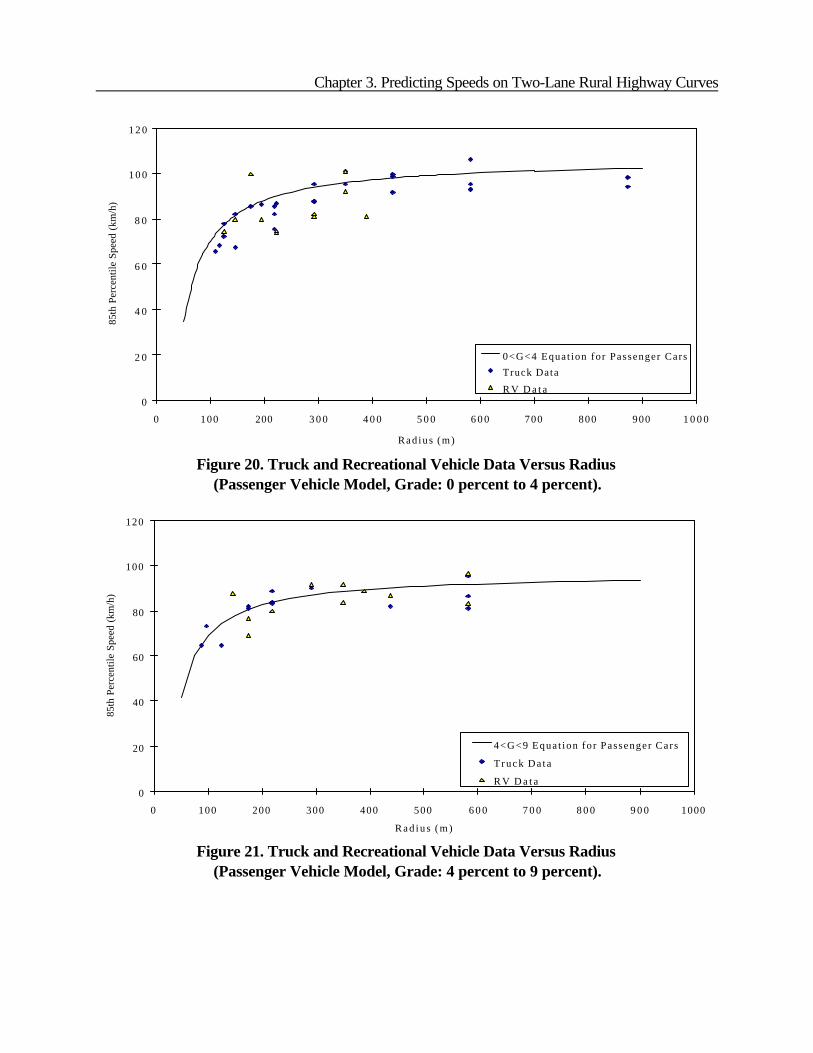
Chapter 3. Predicting Speeds on Two-Lane Rural Highway Curves
0
2 0
4 0
6 0
8 0
1 0 0
1 2 0
0 100 200 3 0 0 4 0 0 5 0 0 6 0 0 700 800 900 1 0 0 0
Rad ius (m)
85th
Per
cent
ile S
peed
(km
/h)
0<G<4 Equat ion for Passenger Cars
Truck Data
R V D a t a
Figure 20. Truck and Recreational Vehicle Data Versus Radius(Passenger Vehicle Model, Grade: 0 percent to 4 percent).
0
20
40
60
80
100
120
0 100 200 300 400 500 6 0 0 7 0 0 8 0 0 9 0 0 1000
R a d i u s ( m )
85th
Per
cent
ile S
peed
(km
/h)
4<G<9 Equa t ion fo r Passenger Cars
Truck Da t a
R V D a t a
Figure 21. Truck and Recreational Vehicle Data Versus Radius(Passenger Vehicle Model, Grade: 4 percent to 9 percent).

Speed Prediction for Two-Lane Rural Highways
0
20
40
60
80
100
120
0 1 0 0 2 0 0 300 400 500 6 0 0 7 0 0 8 0 0 9 0 0 1 0 0 0
Rad ius (m)
85th
Per
cent
ile S
peed
(km
/h)
- 4<G<0 Equat ion for Passenger Cars
Truck Data
RV Data
Figure 22. Truck and Recreational Vehicle Data Versus Radius(Passenger Vehicle Model, Grade: -9 Percent to 0 Percent).
SUMMARY
A primary objective of this research was to develop speed-prediction equations that considercombinations of horizontal and vertical alignment. Regression models were developed for horizontalcurves for different ranges of vertical grade and in combination with sag and limited sight-distance crestvertical curves. They were also developed for limited sight-distance crest vertical curves and sag curveson horizontal tangents. Statistically significant regression equations were not developed for alignmentsthat included non-limited sight-distance crest curves. These findings were based on speed and geometrydata from 103 sites distributed across 6 states (Minnesota, New York, Pennsylvania, Oregon,Washington, and Texas).
Additional objectives of the speed-prediction research were to investigate spiral transitions andother vehicle types. The analyses indicated that spiral transitions did not significantly affect the 85th
percentile speed of vehicles traversing horizontal curves and that any differences between curves withspiral transitions and circular curves were most evident for lower values of curve radius. Because of thelimited amount of data available for truck and recreational vehicles, it is not reasonable to obtainregression equations for these vehicle types for the different alignment conditions. Plots of the truck andRV data compared with plots of the regression equations for passenger cars demonstrated that similartrends exist. Therefore, a design-consistency evaluation method should be based on passenger cars.

4. PREDICTING SPEEDS ON TANGENTSUSING ALIGNMENT INDICES
The objective of this part of this study was to evaluate the applicability of alignment indices asestimators of 85th percentile speeds on long tangents of two-lane rural highways. Alignment indices usethe geometric characteristics of the roadway to provide quantitative measures of the general characterof a roadway’s alignment. It is hypothesized that the previous geometry of the roadway influences thesubsequent speed expectations and desires of motorists. Therefore, these indices, which are based onthe upstream alignment, can possibly reflect the expectancy of motorists when estimating their desiredspeeds on long tangents.
Several approaches have been used to estimate desired speeds on long tangents for speed-based design-consistency evaluations. The most relevant to the current contract is the approach used inthe Australian rural design guide and the approach presented in Report No. FHWA-RD-94-034.(7,57)
McLean performed much of the research that led to the method adopted in the Australiandesign guide for rural roads.(20) McLean was also the first to define desired speed in the way it is usedin this report—“the speed at which drivers choose to travel under free-flow conditions when they arenot constrained by alignment features.”(20) McLean suggested that desired speed was influenced bysuch factors as the purpose of the trip, proximity to urban areas, and the amount of time traffic was onthe road; he also suggested that desired speed was influenced by the geometric characteristics, or theoverall standard of alignment, of the roadway.(20,34) The Australian design guide provides a table ofstandard values for the speed environment of a roadway (i.e., desired speed), based upon McLean’swork, for different terrain types (flat, undulating, hilly, mountainous) and ranges of horizontal curveradii.(57)
Report No. FHWA-RD-94-034 covers attempts to model 85th percentile speeds on longtangents; however, these attempts did not yield a statistically significant model. (7) Independent variablesthat were considered included the travel-way width, total pavement width, characteristics of thepreceding and succeeding curves, tangent length, annual average daily traffic, terrain, and region of thecountry. The only significant difference was between the speeds on long tangents for level terrain inTexas and on long tangents for rolling terrain in the East (New York, Pennsylvania) and West (Oregonand Washington). As a result, the speed-profile model in that publication used a value of 97.9 km/h asthe desired speed on long tangents, the mean of the 85th percentile speeds observed on the 78 longtangents at which data were collected. The use of this mean value does not explain the variability amongobserved 85th percentile speeds at those tangents, which ranged from 85.3 to 112.7 km/h.

Speed Prediction for Two-Lane Rural Highways
CCR 'j ? c%? 1% ? 2
L
PREVIOUS USES OF ALIGNMENT INDICES
While limited research on alignment indices has been performed in the United States, researchefforts on alignment indices have been the focus of other countries, specifically Germany and England.In addition, Polus has examined the issue. These two countries have established methods of usingalignment indices as both a measure of the design consistency and in estimating 85th percentile operatingspeeds.
Germany
In determining the design consistency, Germany uses a parameter for the horizontal alignmentcalled the Curvature Change Rate (CCR). The CCR is the sum of angular changes in the horizontalalignment divided by the length of the highway section. This parameter is used in an attempt to preventunsafe changes in operating speeds and to describe the overall operating characteristics of a road.(19)
The formula below is used to calculate the CCR:(58)
(6)
where: CCR = curvature change rate (deg/km)? C = angular change in circular curve (deg)? 1 = angular change in first transition curve (deg)? 2 = angular change in second transition curve (deg)L = total length of section (km)
In calculating the CCR, the road being examined must be divided into sections that have similaror homogeneous alignments. These sections are determined by plotting the sum of the horizontalcurvature (1/radius) against the length of the entire road. Sections of the alignment that exhibit similarcharacteristics (sections with a similar slope) would be determined subjectively, and the CCR wouldthen be calculated for those sections.(5)
Germany has developed a nomograph that uses the CCR and pavement width to estimate the85th percentile speed over a section of roadway.(22) Extensive investigations have shown that speedcharacteristics on horizontal alignments can be adequately described in terms of the CCR, and thatthere is a strong correlation between the 85th percentile speed of the roadway section and the CCR forall lane widths.(22)
England
England estimates the probable 85th percentile speed on wet pavement conditions based on the

Chapter 4. Predicting Speeds on Tangents Using Alignment Indices
calculated alignment and layout constraints. An estimated 85th percentile speed, which represents acalculated design speed, is inferred from the actual or proposed alignment and cross-section. For newroads, this comparison is used “to identify locations where elements of the trial alignment may berelaxed to achieve cost or environmental savings, or conversely, where the design should be upgraded,according to the calculated design speed.”(59) For existing roadways, this method can be used to determine if and where disparities exist between the design speed stated onroadway plans and probable 85th percentile speeds (which in the English method correspond to acalculated design speed), thereby indicating potential speed inconsistencies.
The alignment constraint measures the degree of constraint imparted by the alignment of theroad and is a function of the bendiness and the harmonic mean visibility. For a two-lane road, thefollowing equation is used to calculate the alignment constraint:(59)
AC = 12 - VISI / 60 + 2B /45 (7)
where:AC = alignment constraintVISI = harmonic mean visibility (m)B = bendiness (deg/km)
Bendiness, identical to the CCR used in Germany, represents the sum of the horizontal angularchanges in the roadway per kilometer. The harmonic mean visibility is the harmonic mean of individualsight-distance observations along the roadway and it should be measured over a minimum sectionlength of 2 km.(59)
The layout constraint measures the degree of constraint imparted by various charac- teristics ofthe roadway and is determined based on roadway type, cross-section width, and access density.(9)
Polus
Polus suggested several alignment indices to quantify the general character of the alignment of aroadway.(60) Indices based on horizontal alignment characteristics included the average curvature indegrees per kilometer, the average radius of curvature, the ratio of the maximum to minimum radius,and two horizontal alignment indices using the radii of curves. Polus also suggested one index based onvertical alignment, the average gradient along a section of roadway. Polus evaluated the correlationbetween these indices and accident rates on 20 segments of roadway in Israel. Among the indicesevaluated, only the ratio of the maximum to the minimum radius was significantly related to the accidentrate. Polus observed that as this value approaches 1, or as the radii of the roads become moreconsistent, a reduced accident rate may be expected.

Speed Prediction for Two-Lane Rural Highways
DEVELOPMENT OF ALIGNMENT INDICES
The hypothesis that alignment indices (representing the character of the preceding alignment)influence drivers’ desired speeds (measured as the 85th percentile speeds on long tangents) wasmotivated by experiences in Australia, Germany, and England. In Australia, desired speeds areestimated based on the terrain and range of the radii of horizontal curvature. In Germany, curvaturechange rate and lane width are used to estimate 85th percentile speeds along a segment of roadway. InEngland, the average speeds along a roadway are estimated based on an alignment constraint(essentially, an alignment index) and a layout constraint (represents the cross-section of the roadway).
Identification of Alignment Indices
The initial step in determining the alignment indices consisted of identifying all possible indicesthat may be useful for this research. Therefore, some of the alignment indices that had been used inother countries or proposed for use were included. In addition, other indices thought to have someworth in estimating the desired speed of motorists on long tangents were developed.
All of these alignment indices could possibly provide an indication of the geometry motoristsexperience upstream on the roadway. Since it is hypothesized that the previous geometry of theroadway influences motorists’ speeds, these indices may be able to quantify the effects of the precedingalignment on the speeds of motorists. A list of the alignment indices that were initially developed for thisstudy is provided in table 18.
Selection of Alignment Indices
As part of this evaluation, some of the proposed alignment indices in table 18 were computedfor a small sample of roadways. After examining these results and the proposed alignment indices moreclosely, it was determined that some of the indices may be more worthwhile for use in estimating thedesired speeds of motorists on long tangents than others. Two other criteria used in determiningwhether the indices should be further evaluated in this study were:
• Alignment indices had to be strictly a function of the geometry of a roadway.• There had to be a reasonable hypothesized relationship between the alignment index and the
85th percentile speeds.
Therefore, those indices that were thought to be better measures were evaluated in this research whilethe others were eliminated from consideration. The rationale used in making these decisions isdescribed in the following sections.

Chapter 4. Predicting Speeds on Tangents Using Alignment Indices
Table 18. Initial Alignment Indices Identified.Horizontal Alignment Indices1. Angular Change in Direction
• Average Deflection Angle per Length(Bendiness or Curvature Change Rate)
• Average Deflection Angle per Curve• Average Degree of Curvature per Length• Average Degree of Curvature per Curve• Ratio of Curve Length to Total Roadway
Length2. Radii Measures
• Average Radius• Average Radius / Minimum Radius• Maximum Radius / Minimum Radius
3. Tangent Length• Average Tangent Length
4. Sight Distance• Harmonic Mean Visibility
Vertical Alignment Indices1. Angular Change in Direction
• Algebraic Difference in Grades / Length(Percent per Kilometer)(Degrees per Kilometer)
• Average Rate of Vertical Curvature2. Elevation Measures
• Average Gradient3. Sight Distance
• Sight Distance
Composite Alignment Indices1. Angular Change in Direction2. Average Highway Speed
Horizontal
The length-based alignment indices for the horizontal angular change in direction were selectedfor further evaluation. Since the length-based indices consider the length of the roadway, it wasassumed that these alignment indices were more representative of the general character of the alignmentof the roadway. The average deflection angle and average degree of curvature per curve were notevaluated further for the horizontal alignment indices using the angular change in direction because theGermans and English both calculate their indices on a per length basis rather than based on the numberof features. Furthermore, using the average radius as an alignment index would provide similarinformation to these feature-based indices. For example, stating that the previous 3 km of roadway hada degree of curvature alignment index value of 12 deg/km describes the angular change motoristsexperience better than simply stating that the average degree of curve for the same distance was 5degrees. A large value for these indices indicates that the road either contains a large number of curvesor there are long or sharp curves in that section. It was expected that an increase in the value of theseindices would decrease the desired speeds of motorists.
Correspondingly, the ratio of curve length to total roadway length was selected because it couldalso provide a good indication of the character of the alignment. This alignment index providesinformation on the proportion of the roadway that is on curved sections. As the road includes morecurves or longer curves, this proportion increases, and the speeds motorists drive would be expected to

Speed Prediction for Two-Lane Rural Highways
decrease.
The horizontal indices that compare the ratio of the average and maximum radii to the minimumradius were not chosen for further evaluation. While these indices appear to provide indications ofdesign consistency rather well (the closer the value is to 1, the more consistent the design), it wasthought that these indices did not quantitatively represent the character of the roadway adequately topredict speeds on tangents. For example, a value of 2 may be the ratio between either a 1,746-m (1-deg) and a 873-m (2-deg) curve or a 350-m (5-deg) and a 175-m (10-deg) curve. It is hypothesizedthat motorists would react differently to each situation, thereby making speed estimation difficult.
The average radius and average tangent length were selected for further study because theycould represent what a driver would typically experience along sections of the previous alignment. Theaverage radius expresses what motorists typically encounter on curved sections of the road. A largeaverage radius would indicate curves that are typically not very sharp. Therefore, it is expected thathigher speeds would exist for these values compared to smaller average radius values. The averagetangent length indicates the length of tangent that is typically available to motorists between curvedsections of the roadway. A large value for this index would indicate that the road has tangent sectionsthat are typically long, therefore, motorists’ speeds would be expected to be higher than for roads witha smaller value.
The use of a sight-distance-based alignment index in the horizontal plane was not consideredfurther because an automated method of calculating the actual sight-distance available to the motoristsfrom roadway design plans was not available. In addition, the amount of sight distance available tomotorists is based on subjective parameters, such as driver eye height and object height. The intent ofthis research was to use alignment indices that were geometry-based.
Table 19 provides a list of the horizontal alignment indices selected for use in this study. Thistable also shows the equations necessary to compute the indices and the indices’units.
Vertical
For the vertical alignment indices, all the indices initially developed were studied further exceptfor vertical sight distance. Sight distance as a vertical alignment index was not selected because anautomated method of calculating the actual sight distance available to the motorists from roadwaydesign plans does not exist. In addition, the sight distance available to motorists is not based on thegeometric parameters of the road, but rather it uses subjective parameters such as driver eye height andobject height.
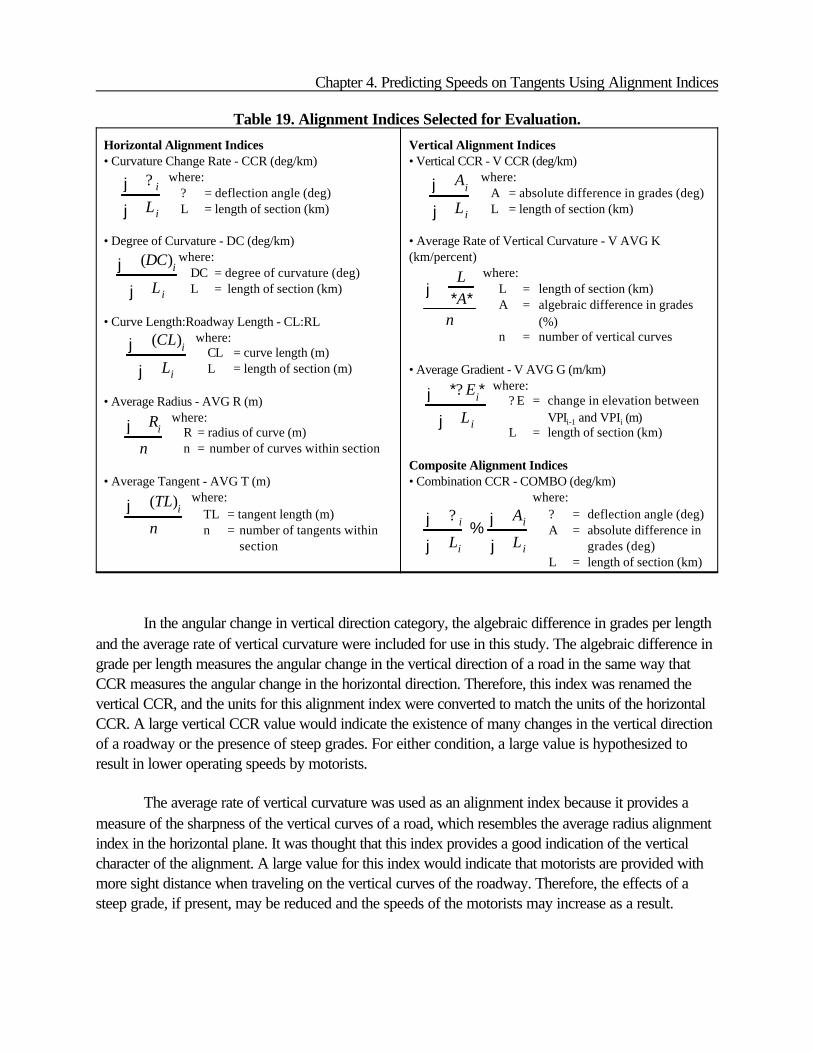
Chapter 4. Predicting Speeds on Tangents Using Alignment Indices
j ? i
j L i
j (DC)i
j L i
j (CL)i
j Li
j Ri
n
j (TL)i
n
j Ai
j L i
j L*A*
n
j *? Ei*
j L i
j ? i
j Li
%j Ai
j L i
Table 19. Alignment Indices Selected for Evaluation.
Horizontal Alignment Indices• Curvature Change Rate - CCR (deg/km)
where:? = deflection angle (deg)L = length of section (km)
• Degree of Curvature - DC (deg/km)where:
DC = degree of curvature (deg)L = length of section (km)
• Curve Length:Roadway Length - CL:RLwhere:
CL = curve length (m)L = length of section (m)
• Average Radius - AVG R (m)where:
R = radius of curve (m)n = number of curves within section
• Average Tangent - AVG T (m)where:
TL = tangent length (m)n = number of tangents within
section
Vertical Alignment Indices• Vertical CCR - V CCR (deg/km)
where:A = absolute difference in grades (deg)L = length of section (km)
• Average Rate of Vertical Curvature - V AVG K(km/percent)
where:L = length of section (km)A = algebraic difference in grades
(%)n = number of vertical curves
• Average Gradient - V AVG G (m/km)where:
? E = change in elevation betweenVPIi-1 and VPIi (m)
L = length of section (km)
Composite Alignment Indices • Combination CCR - COMBO (deg/km)
where:? = deflection angle (deg)A = absolute difference in
grades (deg)L = length of section (km)
In the angular change in vertical direction category, the algebraic difference in grades per lengthand the average rate of vertical curvature were included for use in this study. The algebraic difference ingrade per length measures the angular change in the vertical direction of a road in the same way thatCCR measures the angular change in the horizontal direction. Therefore, this index was renamed thevertical CCR, and the units for this alignment index were converted to match the units of the horizontalCCR. A large vertical CCR value would indicate the existence of many changes in the vertical directionof a roadway or the presence of steep grades. For either condition, a large value is hypothesized toresult in lower operating speeds by motorists.
The average rate of vertical curvature was used as an alignment index because it provides ameasure of the sharpness of the vertical curves of a road, which resembles the average radius alignmentindex in the horizontal plane. It was thought that this index provides a good indication of the verticalcharacter of the alignment. A large value for this index would indicate that motorists are provided withmore sight distance when traveling on the vertical curves of the roadway. Therefore, the effects of asteep grade, if present, may be reduced and the speeds of the motorists may increase as a result.

Speed Prediction for Two-Lane Rural Highways
The average gradient was included for evaluation because this index represented the absolutechange in vertical direction along a roadway. As the average gradient increases in value, this indicatesthat either there is typically a large change in elevation between the vertical point of intersections or thatthe vertical alignment is hilly. It is hypothesized that a large value for this index would result in lowoperating speeds.
Table 19 shows the vertical alignment indices evaluated in this study. The equations used tocalculate the indices and their units are also included. Although Germany and England do not considervertical alignment indices in their design practices, this research attempts to use vertical alignmentindices in estimating the desired speeds of motorists on long tangents. One weakness associated withthese vertical alignment indices is that they treat crest and sag vertical curves equally. This equaltreatment is a concern because each type of vertical curve has a different effect on the speeds ofmotorists. Since crest curves typically limit the sight distance of motorists more so than sag curves, crestvertical curves may have a greater effect on the speeds of motorists. In the evaluation of the verticalalignment indices, these effects must be considered.
Composite
Of the two composite alignment indices identified, the average highway speed was eliminatedfrom consideration because it is based on the design speed of the individual alignment elements of theroadway. While this index uses the geometric characteristics of the road, it also utilizes the design-speed concept. As discussed previously, there are several weaknesses of the design-speed conceptthat hinder its ability to ensure operating-speed consistency, and thus, its ability to estimate speeds ofmotorists on long tangents.
The composite angular change in direction combines the horizontal and vertical angular changein direction of the roadway. This index was termed the combination CCR because it was computed bysimply adding the horizontal CCR value and the vertical CCR value. As the value of the combinationCCR increased, indicating more angular changes in either the horizontal and/or vertical direction of theroadway, it was hypothesized that the speeds of motorists would tend to decrease.
In evaluating this index, it is important to note that the total angular change in the horizontaldirection is much greater than the total angular change in the vertical direction. Therefore, by simplyadding these two effects, greater emphasis is placed on the effect of the horizontal alignment than thevertical alignment. While it is assumed that the horizontal alignment plays a greater role in thedetermination of speeds, the magnitude of this effect is not known. The composite alignment index beingevaluated is shown in table 19. The units for this index and the equation are also shown.

Chapter 4. Predicting Speeds on Tangents Using Alignment Indices
ANALYSIS METHODOLOGY
Identification of Geometric Variables
In addition to the alignment indices, other geometric characteristics thought to influence thedesired speeds of motorists on long tangents were identified. Five independent variables identified forevaluation were vertical grade at the tangent site, total pavement width at the tangent site, roadsidehazard rating, driveway density, and the posted speed limit of the roadway.
The vertical grade on the tangent was examined because the vertical grade of the roadway canhave an effect on the speeds that motorists drive. It was hypothesized that the 85th percentile speedswould be lower for approach tangents to horizontal curves on upgrades compared to tangents ondowngrades. More specifically, the steeper the upgrade, the more reduction in speed is expected.
It was also hypothesized that as the total pavement width at the tangent site increased, thespeeds of motorists would also tend to increase. Wider pavements on the roadway would allowmotorists more room to maneuver their vehicles along the road. Motorists may feel more comfortabledriving faster at locations where extra space exists between them and other vehicles on one side and thepavement edge on the other.
The consequences of running off the road increase in severity as the roadside hazard ratingincreases. Therefore, it was hypothesized that desired speeds would decrease as the roadside hazardrating increased. A seven-point scale was used to describe the roadway surroundings with 1representing a clear roadside and 7 representing severe roadside hazards.
Driveway density is a measure of the roadside friction associated with adjacent landdevelopment. It was hypothesized that desired speeds would decrease as driveway density increases.Since rural areas are characterized by low driveway densities, it was further hypothesized that desiredspeeds would not be sensitive to driveway densities within the range of values at the sites in this study.
A logical relationship exists between the posted speed limit of a roadway and the speedsmotorists want to drive. As the legal speed limits increase, the 85th percentile speeds of motorists areexpected to increase. Motorists tend to drive at or above the speed limit of a roadway.
Because of the relationships described above, these five independent variables were analyzedtogether with the alignment indices to determine their ability to predict desired speeds of motorists. Itwas hypothesized that either one or more of these variables could be used in addition to the alignmentindices in predicting the desired speeds of motorists on long tangents of two-lane rural highways.

Speed Prediction for Two-Lane Rural Highways
The factors mentioned above are only a few of the possible influences on motorists’ desiredspeeds on long tangents of two-lane rural highways. Other characteristics of the roadway may play arole in the speeds motorists drive on tangents. These characteristics include items such as:
• Familiarity of roadway to motorist.• Available sight distance to the motorist.• Available roadside clear distance.
However, these factors are difficult to quantify and were not investigated in this research.
Data Collection and Reduction
For this effort, the spot-speed and roadway alignment data collected for other tasks were used;these data were described in chapter 3. Alignment data were extracted from highway design plansobtained from the corresponding State’s department of transportation and geometric characteristicswere collected in the field. Table 20 shows the data that were required from the roadway plans in orderto compute the alignment indices. The roadway design plans were converted into a computerizedspreadsheet format and were used to efficiently calculate the alignment indices.
Table 20. Alignment Data Required From Highway Design Plans.Horizontal Vertical
Station of PCStation of PTTangent LengthCurve LengthRadiusDegree of CurveDeflection Angle
Station of Vertical PCStation of Vertical PIStation of Vertical PTGradesCurve LengthAlgebraic Difference in GradesRate of Vertical CurvatureElevation of Vertical PI
Alignment indices were computed for only 68 of the 176 sites available. The number of siteswas reduced because the sites had to meet the criteria listed below:
• Available speed data for the horizontal curve site.• Available speed data on the preceding tangent of a horizontal curve site.• Identified tangent had to be considered an independent tangent.• Selected preceding tangent length of curve site must be greater than 200 m.

Chapter 4. Predicting Speeds on Tangents Using Alignment Indices
TLC '2V 2
f & V85 21 & V85 2
2
25.92 a
An independent tangent is classified in the speed-profile model as a tangent that is long enoughfor motorists to accelerate to and maintain their desired speed for some distance. The equation below,which considers the degree of curvature preceding and following the tangent, was developed for use inthe speed-profile model to determine whether a tangent could be considered an independent tangent:(7)
(8)
where: TLc = critical tangent length (m)Vf = 85th percentile desired speed on long tangents = 97.9 km/hV85n = 85th percentile speed on curve n (km/h)a = acceleration/deceleration = 0.85 m/s2
In this equation, the critical tangent length represents the length of tangent necessary formotorists to accelerate to and maintain their desired speed. If the actual tangent lengths were greaterthan the critical tangent length value, then a desired speed could be reached on that particular tangent.The tangents used in this study satisfied this criterion.
In addition to being considered an independent tangent, the length of the tangent had to begreater than 200 m. Two factors influenced the selection of this limiting value. First, a previous study ontangent speeds of two-lane rural highways considered a tangent length of 244 m as an independenttangent.(7) Second, a visual inspection of a plot of 85th percentile tangent speeds against tangent length,shown in figure 23, appeared to reveal that speeds on a tangent became constant after a tangent lengthof 200 m. The slope of a linear regression line using tangent lengths greater than 200 m was notsignificantly different from zero.
Statistical Analysis
Several techniques were utilized in analyzing the data collected for this study. A graphicalanalysis was performed to provide an initial visual indication of any relationships that may exist betweenthe 85th percentile tangent speeds and the alignment indices. After examining the graphical analysisresults, a simple linear regression analysis was performed to determine if one of the alignment indiceswas a significant predictor of desired speeds. This analysis was used to confirm or deny the existence ofrelationships that may have been determined visually through the graphical analysis. Geometric variableswere then introduced to determine if they could be used in combination with alignment indices toestimate the desired speeds of motorists. A correlation analysis was then used in determining if anyrelationships existed among the alignment indices and the geometric variables. The results of thisanalysis were used in the multiple linear regression analysis that followed. If any of the alignment indicesor geometric variables were correlated, then they should not be included as predictors in the same

Speed Prediction for Two-Lane Rural Highways
multiple regression model. The multiple linear regression analysis determined which indices andgeometric variables may be useful in combination to predict the desired speeds of motorists. After allthe possible relationships between the 85th percentile speeds and alignment indices were examined, ananalysis of variance (ANOVA) was performed to determine if there were significant differences in theobserved 85th percentile speeds due to the geometric variables of vertical grade, total pavement width,posted speed, driveway density, and roadside rating. In addition, this analysis was also used todetermine if there were regional differences in the observed 85th percentile tangent speeds. All of thestatistical analyses were performed using SAS® and were tested at a 90-percent confidence interval(i.e., significance level of a = 0.10).
.
0
20
40
60
80
100
120
140
0 200 400 600 800 1000 1200 1400
Preceding Horizontal Tangent Length (meters)
85th
Per
cen
tile
Tan
gen
t S
pee
d (
km/h
)
Figure 23. Observed 85th Percentile Tangent Speeds Versus Preceding HorizontalTangent Length.

Chapter 4. Predicting Speeds on Tangents Using Alignment Indices
RESULTS
Summary of Site Characteristics and Values
There were 68 sites in this study that satisfied the criteria mentioned previously. These siteswere located in six States (see table 21). The geometric and speed characteristics at each tangent sitewere either collected in the field or obtained from roadway design plans. A summary of thesecharacteristics for this study is presented in table 22. Ranges of values for the alignment indices using 5km of the preceding roadway alignment are shown in table 23.
Table 21. Number of Sites by State.State No. of Sites No. of Road Segments
Minnesota 2 2
New York 9 3
Oregon 21 4
Pennsylvania 8 3
Texas 13 7
Washington 15 7
Total 68 26
Table 22. Summary of Site Characteristics.Minimum Maximum Average
Tangent Length (m) 201.4 1368.8 485.0
Preceding Roadway Alignment Available (km) 0.1 23.6 8.2
Grade on Tangent (%) -9.0 8.0 0.6
Total Pavement Width (m) 6.2 12.7 8.0
Posted Speed (km/h) 80.5 112.7 89.3
Observed 85th Percentile Tangent Speed (km/h) 80.0 121.7 96.8
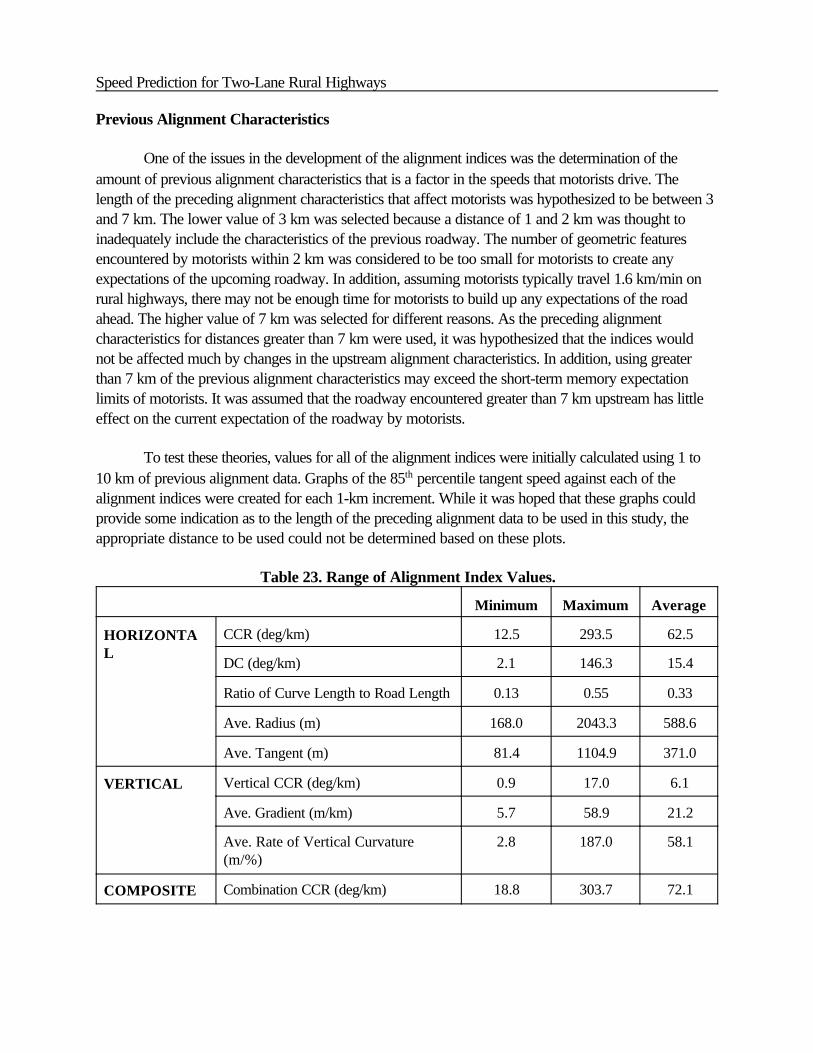
Speed Prediction for Two-Lane Rural Highways
Previous Alignment Characteristics
One of the issues in the development of the alignment indices was the determination of theamount of previous alignment characteristics that is a factor in the speeds that motorists drive. Thelength of the preceding alignment characteristics that affect motorists was hypothesized to be between 3and 7 km. The lower value of 3 km was selected because a distance of 1 and 2 km was thought toinadequately include the characteristics of the previous roadway. The number of geometric featuresencountered by motorists within 2 km was considered to be too small for motorists to create anyexpectations of the upcoming roadway. In addition, assuming motorists typically travel 1.6 km/min onrural highways, there may not be enough time for motorists to build up any expectations of the roadahead. The higher value of 7 km was selected for different reasons. As the preceding alignmentcharacteristics for distances greater than 7 km were used, it was hypothesized that the indices wouldnot be affected much by changes in the upstream alignment characteristics. In addition, using greaterthan 7 km of the previous alignment characteristics may exceed the short-term memory expectationlimits of motorists. It was assumed that the roadway encountered greater than 7 km upstream has littleeffect on the current expectation of the roadway by motorists.
To test these theories, values for all of the alignment indices were initially calculated using 1 to10 km of previous alignment data. Graphs of the 85th percentile tangent speed against each of thealignment indices were created for each 1-km increment. While it was hoped that these graphs couldprovide some indication as to the length of the preceding alignment data to be used in this study, theappropriate distance to be used could not be determined based on these plots.
Table 23. Range of Alignment Index Values.
Minimum Maximum Average
HORIZONTAL
CCR (deg/km) 12.5 293.5 62.5
DC (deg/km) 2.1 146.3 15.4
Ratio of Curve Length to Road Length 0.13 0.55 0.33
Ave. Radius (m) 168.0 2043.3 588.6
Ave. Tangent (m) 81.4 1104.9 371.0
VERTICAL Vertical CCR (deg/km) 0.9 17.0 6.1
Ave. Gradient (m/km) 5.7 58.9 21.2
Ave. Rate of Vertical Curvature(m/%)
2.8 187.0 58.1
COMPOSITE Combination CCR (deg/km) 18.8 303.7 72.1

Chapter 4. Predicting Speeds on Tangents Using Alignment Indices
To adequately determine the effect that the previous alignment data had on the alignmentindices, figure 24 was developed. This figure represents the average change in the horizontal, vertical,and composite alignment indices from the previous 1-km increment. This figure shows that after adistance of 5 km, the values of the alignment indices remain constant; therefore, using alignmentcharacteristics greater than 5 km upstream of the tangent site does not significantly change the value ofthe indices. In addition, analyses of the results using upstream distances of 1 to 10 km were similar tothe results obtained for 5 km of upstream alignment. Therefore, alignment characteristics a distance of 5km upstream of and including the tangent site were used and reported for the remaining analyses in thisstudy. Using this distance, the sample size of tangent sites was reduced from 68 to 40 for the horizontalalignment indices and to 35 for the vertical alignment indices.
The sample size was reduced from the original 68 sites because the length of the precedingalignment data available varied by individual roads. As the amount of preceding alignment distancebeing used increased, the number of available tangent sites decreased. In addition, there were fewertangent sites for the vertical alignment indices because several of the roadway design plans did notcontain any vertical alignment information.
-20
0
20
40
60
80
100
120
140
2 3 4 5 6 7 8 9 10
Distance (km)
Per
cen
t C
han
ge
(%)
HorizontalVerticalComposite
Figure 24. Average Change in Alignment Indices by Distance.

Speed Prediction for Two-Lane Rural Highways
0
20
40
60
80
100
120
140
0 50 100 150 200 250 300
CCR (degrees/km)
85th
Per
cent
ile T
ange
nt S
peed
(km
/h)
Figure 25. 85th Percentile Tangent Speed Versus CCR.
Examination of Alignment Indices as Individual Estimators of Desired Speed
In determining whether any of the alignment indices were able to individually predict 85th
percentile tangent speeds on long tangents of two-lane rural highways, graphical and simple linearregression analyses were used. The graphical analysis was performed initially to assist the regressionanalysis.
Graphical Analysis
The ability of individual alignment indices to predict the 85th percentile tangent speeds was firstexamined graphically. For all nine of the alignment indices, graphs of the observed 85th percentiletangent speeds against the alignment indices were developed. These graphs, which are shown in figures25 through 33, were created in order to visually inspect those indices that may have promise inestimating the desired speeds of motorists on long tangents.

Speed Prediction for Two-Lane Rural Highways
0
20
40
60
80
100
120
140
0 0.1 0.2 0.3 0.4 0.5 0.6
Curve Length:Road Length
85th
Per
cen
tile
Tan
gen
t S
pee
d (
km/h
)
Figure 27. 85th Percentile Tangent Speed Versus Ratio of Curve Length toRoad Length.
0
20
40
60
80
100
120
140
0 500 1000 1500 2000 2500
Average Radius (meters)
85th
Per
cen
tile
Tan
gen
t S
pee
d (
km/h
)
Figure 28. 85th Percentile Tangent Speed Versus Average Radius.

Chapter 4. Predicting Speeds on Tangents Using Alignment Indices
0
20
40
60
80
100
120
140
0 200 400 600 800 1000 1200
Average Tangent (meters)
Figure 29. 85th Percentile Tangent Speed Versus Average Tangent.
0
20
40
60
80
100
120
140
0 2 4 6 8 10 12 14 16 18
Vertical CCR (degrees/km)
85th
Per
cen
tile
Tan
gen
t Sp
eed
(km
/h)
Figure 30. 85th Percentile Tangent Speed Versus Vertical CCR.

Speed Prediction for Two-Lane Rural Highways
0
20
40
60
80
100
120
140
0 20 40 60 80 100 120 140 160 180 200
Average Rate of Vertical Curvature (meters/%)
85th
Per
cen
tile
Tan
gen
t Sp
eed
(km
/h)
Figure 31. 85th Percentile Tangent Speed Versus Average Rate of Vertical Curvature.
0
20
40
60
80
100
120
140
0 10 20 30 40 50 60
Average Gradient (meters/km)
85th
Per
cen
tile
Tan
gen
t S
pee
d (
km/h
)
Figure 32. 85th Percentile Tangent Speed Versus Average Gradient.

Chapter 4. Predicting Speeds on Tangents Using Alignment Indices
0
20
40
60
80
100
120
140
0 50 100 150 200 250 300 350
Combination CCR (degrees/km)
85th
Per
cen
tile
Tan
gen
t S
pee
d (
km/h
)
Figure 33. 85th Percentile Tangent Speed Versus Combination CCR.
From these graphs, there appeared to be a relationship between the 85th percentile speeds andseveral of the alignment indices. The apparent relationships are indicated below:
• As the curvature change rate increased, the 85th percentile tangent speeds decreased.• As the degree of curvature index increased, the 85th percentile tangent speeds decreased.• As the average radius increased, the 85th percentile tangent speeds increased.• As the average tangent increased, the 85th percentile tangent speeds increased.• As the vertical CCR increased, the 85th percentile tangent speeds decreased.• As the combination CCR increased, the 85th percentile tangent speeds decreased.
The relationships that were identified from the graphs were consistent with the hypothesizedrelationships discussed in the development of the alignment indices. However, most of the trendsobserved in these graphs appeared to be slight, indicating that the alignment indices did not have muchof an effect, if any, on the desired speeds of motorists on long tangents. Finally, several of therelationships suggested by these graphs appeared to be influenced by one or more extreme values.
Simple Linear Regression Analysis
To determine whether there was a statistically significant relationship (at a = 0.10) between the85th percentile tangent speeds and these alignment indices as shown in the graphs, simple linearregression analyses were performed. The results of the regression analyses are listed in table 24.
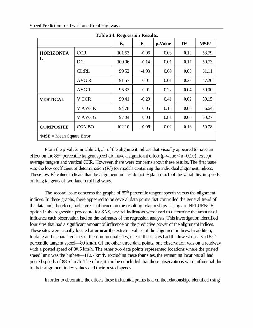
Speed Prediction for Two-Lane Rural Highways
Table 24. Regression Results.
ß0 ß1 p-Value R2 MSEa
HORIZONTAL
CCR 101.53 -0.06 0.03 0.12 53.79
DC 100.06 -0.14 0.01 0.17 50.73
CL:RL 99.52 -4.93 0.69 0.00 61.11
AVG R 91.57 0.01 0.01 0.23 47.20
AVG T 95.33 0.01 0.22 0.04 59.00
VERTICAL V CCR 99.41 -0.29 0.41 0.02 59.15
V AVG K 94.78 0.05 0.15 0.06 56.64
V AVG G 97.04 0.03 0.81 0.00 60.27
COMPOSITE COMBO 102.10 -0.06 0.02 0.16 50.78
aMSE = Mean Square Error
From the p-values in table 24, all of the alignment indices that visually appeared to have aneffect on the 85th percentile tangent speed did have a significant effect (p-value < a=0.10), exceptaverage tangent and vertical CCR. However, there were concerns about these results. The first issuewas the low coefficient of determination (R2) for models containing the individual alignment indices.These low R2-values indicate that the alignment indices do not explain much of the variability in speedson long tangents of two-lane rural highways.
The second issue concerns the graphs of 85th percentile tangent speeds versus the alignmentindices. In these graphs, there appeared to be several data points that controlled the general trend ofthe data and, therefore, had a great influence on the resulting relationships. Using an INFLUENCEoption in the regression procedure for SAS, several indicators were used to determine the amount ofinfluence each observation had on the estimates of the regression analysis. This investigation identifiedfour sites that had a significant amount of influence on the predictive power of the alignment indices.These sites were usually located at or near the extreme values of the alignment indices. In addition,looking at the characteristics of these influential sites, one of these sites had the lowest observed 85th
percentile tangent speed—80 km/h. Of the other three data points, one observation was on a roadwaywith a posted speed of 80.5 km/h. The other two data points represented locations where the postedspeed limit was the highest—112.7 km/h. Excluding these four sites, the remaining locations all hadposted speeds of 88.5 km/h. Therefore, it can be concluded that these observations were influential dueto their alignment index values and their posted speeds.
In order to determine the effects these influential points had on the relationships identified using

Chapter 4. Predicting Speeds on Tangents Using Alignment Indices
these observations, simple linear regression analyses were performed again without including these fourdata points. These analyses were also performed to see whether the results obtained without theinfluential observations were the same as the results obtained including the influential observations.
The results of these simple regression analyses are in table 25. The results show that none of thealignment indices were statistically significant predictors of 85th percentile tangent speeds. In addition,the coefficient of determination was near zero for all of the alignment indices. These results indicate thatat a significance level of a = 0.10, none of the alignment indices were individually able to estimate the85th percentile tangent speeds of motorists.
After further examining the results of the simple linear regression analyses, it was decided thatthe influential observations were to be excluded from the data sets. With such limited data available atthe extreme values, it was difficult to accept with confidence the results that were obtained by includingthese extreme values. Based on the regression results without the influential observations, it wasdetermined that none of the alignment indices were significant predictors of the 85th percentile speeds ofmotorists.
Table 25. Regression Results Without Influential Points.
ß0 ß1 p-Value R2 MSE
HORIZONTAL
CCR 97.18 0.01 0.77 0.00 30.26
DC 99.12 -0.10 0.37 0.02 29.61
CL:RL 93.11 13.59 0.19 0.05 28.79
AVG R 97.03 0.00 0.71 0.00 30.21
AVG T 97.15 0.00 0.76 0.00 30.25
VERTICAL V CCR 98.22 -0.12 0.61 0.01 23.57
V AVG K 96.87 0.01 0.64 0.01 23.60
V AVG G 95.94 0.07 0.35 0.03 23.08
COMPOSITE COMBO 97.12 0.01 0.86 0.00 23.76
Examination of a Multiple Linear Regression Model in Estimating Desired Speed
Since none of the alignment indices were determined to individually predict the 85th percentilespeeds for motorists on tangents in the simple linear regression analyses, the use of a combination ofalignment indices and geometric variables as predictors in a multiple linear regression model wasexamined. However, the use of posted speed as an independent variable was not considered here,

Speed Prediction for Two-Lane Rural Highways
because all the sites had the same posted speed (88.5 km/h). Stepwise multiple linear regressionanalysis was performed to determine if any combination of variables could estimate 85th percentilespeeds. These results are in table 26.
The results provided a multiple linear regression model that appears to be adequate inpredicting the 85th percentile tangent speed of motorists. All of the p-values were significant and themodel R2 of 0.51 was acceptable; however, this suggested model contains independent variables thatwere identified as being highly correlated. The variables in this model that were highly correlated arelisted below and should not be used in the same model:
• Ratio of Curve Length to Road Length and Average Tangent.• Average Tangent and Average Gradient.
Using a combination of the four variables suggested by the stepwise multiple linear regressionresults, and not including the highly correlated variables together in the same model, multiple regressionanalyses were performed again. The results of these analyses are in table 27.
Table 26. Stepwise Multiple Regression Analysis Results.
Model Variable Entered R2 p-Value MSE
Partial Model
1 CL:RL 0.12 0.12 0.05 20.83
2 AVG T 0.19 0.32 0.01 16.79
3 WIDTH 0.13 0.44 0.02 14.18
4 V AVG G 0.06 0.51 0.07 13.04
Only one of these models that used combinations of the four variables was determined to be asignificant estimator of 85th percentile speeds. According to the p-values of the variables, the modelcontaining the ratio of curve length to road length alignment index and the total pavement width wassignificant; however, there were two concerns with using this model to predict speeds. The first concernwas the low R2 value (0.14) associated with this model. The second concern was that the signs of theparameter estimates were counter-intuitive. This model indicates that as motorists drive a higherproportion of curves along the road, their speeds on long tangents will increase; however, a curvilinearalignment is believed to reduce operating speeds. Although once a driver reaches a long tangent after aseries of curves, a higher speed could result because the driver welcomes the opportunity to be able todrive faster. In addition, however, this model indicates that as the total pavement width of the roadwayincreases, the desired speed of motorists on long tangents decreases. In requirements for minimum lane

Chapter 4. Predicting Speeds on Tangents Using Alignment Indices
and shoulder width values for two-lane rural highways, previous research suggests that widerpavements usually result in higher operating speeds by motorists.(60) Due to these concerns, it wasdetermined that a model including only these two variables to estimate desired speeds on long tangentswas not acceptable.
Possible Influences on Desired Speed
The results from the previous sections indicated that none of the alignment indices examinedwere able to predict the desired speeds of motorists on long tangents, even in combination withgeometric variables. Therefore, this section considers other factors and variables that may have aninfluence on the speeds motorists drive on long tangents. In examining these influences, all 68 tangentsites were included unless otherwise stated.
Regional Speed Differences
The mean 85th percentile speeds of the different regions in this study were examined todetermine if there was a difference in the speed characteristics of motorists by region. Regionaldifferences in speed may be attributed to the different alignment and motorist characteristics that arebelieved to exist in different locations across the United States. Table 28 lists the mean 85th percentiletangent speeds from each State.
Table 27. Multiple Regression Analysis Results.
Model CL:RL AVG T V AVG G WIDTH R2 MSE ß0No. of Obs.
1 ß1 13.590.05 28.79 93.11 36
p-value 0.19
2 ß1 17.87 -1.250.14 26.89 101.53 36
p-value 0.08 0.07
3 ß1 18.96 0.050.14 21.27 89.65 31
p-value 0.07 0.54
4 ß1 30.99 0.04 -1.700.28 18.36 98.91 31
p-value 0.01 0.62 0.03
5 ß1 0.0020.00 30.25 97.15 36
p-value 0.76
6 ß1 0.002 -0.960.06 29.45 104.87 36
p-value 0.79 0.17

Speed Prediction for Two-Lane Rural Highways
Table 28. 85th Percentile Speeds on Long Tangents by State.State No. of Sites 85th Percentile Tangent Speed (km/h)
Minnesota 2 99.2
New York 9 93.2
Oregon 21 96.3
Pennsylvania 8 93.1
Texas 13 (9)* 104.3 (103.2)
Washington 15 94.8
* Nine of the Texas sites had posted speeds of 88.5 km/h or less and four hadposted speeds greater than 88.5 km/h.
Performing an analysis of variance on these results, it was determined that the 85th percentilespeeds for long tangents in Texas significantly differed from all of the other States, except Minnesota.These speed differences may be due to the presence of four sites in Texas that had posted speedsgreater than 88.5 km/h. In addition, factors such as the roadside clear zone and the familiarity ofmotorists with the roads are two other possibilities for this speed difference between Texas and theother States.
In a previous study, differences in 85th percentile speeds by region were also examined.(7) Theprevious research used the same States as in this study, with the exception of Minnesota, andinvestigated tangents greater than 244 m in length. Table 29 provides a comparison between theprevious results and this research. In order to provide a fair comparison to the previous research, theresults from this study were grouped into the same regions used in the previous research, and onlytangent lengths greater than 244 m from this current research were used. In addition, only roads withposted speeds of 80.5 km/h and 88.5 km/h from the current research were included, since these werethe posted speeds examined in the previous research.
Table 29. Comparison of Regional Differences in 85th Percentile Tangent Speeds.
Region
Previous Study(7) Current Researcha
Grade Between -5and +5 percent
All GradesGrades Between -5
and +5 percent
Speed (km/h)
Speed(km/h)
No. ofSites
Speed(km/h)
No. ofSites

Chapter 4. Predicting Speeds on Tangents Using Alignment Indices
South 99.8 105.3 7 105.3 7
East and West 96.0 95.5 49 96.4 43
All Regions 97.9 96.7 56 97.7 50a Includes sites with tangent lengths greater than 244 m and posted speeds of 80.5 or 88.5 km/h.
The East and West region combined the results of New York, Oregon, Pennsylvania, andWashington speed data. The South region consisted of speed data in Texas. Based on the results ofthese two studies, it appears that there are State variations in the desired speeds of motorists on longtangents. Analysis of variance of these results confirmed that 85th percentile speeds on long tangents inTexas were significantly greater than the 85th percentile speeds for the other States.
Further comparison of the results of these two studies indicates that the means of the 85th
percentile speeds on long tangents of two-lane rural highways were similar (97.9 and 96.7 km/h). A t-test was performed to compare these two means, and the results indicated no significant difference inthe 85th percentile tangent speeds for these two studies. In addition, including tangents greater than 200m in this study, the mean of the 85th percentile tangent speeds (96.2 km/h) was also not significantlydifferent from the previous research. Therefore, the estimate of the desired speeds of motorists on longtangents used in the speed-profile model (97.9 km/h) should be retained under the following conditions:
• Tangent lengths > 200 m.• Posted speed = 88.5 km/h.
Total Pavement Width
The total pavement width at the tangent sites for this study ranged from 6.2 to 12.7 m. Figure34 is a plot of the 85th percentile tangent speeds against the total pavement width for the 68 tangentsites. For analyzing the pavement width data, the widths were classified into three levels. These levelsdivided the width of the roadways into three categories: narrow, average, and wide. It washypothesized that if there were any differences in speeds, they would exist between the narrowest andwidest pavement widths. These classes of pavement width and their respective means are shown intable 30.
Analysis of variance results indicates that the mean 85th percentile tangent speeds for theseclasses of widths were not significantly different from each other (p-value = 0.2614). Although travel-way width was found to be a significant predictor of 85th percentile speeds on tangents in other studies,this research indicated that total pavement width was not a significant predictor of desired speeds ofmotorists on long tangents of two-lane rural highways.(15,62) A previous study also investigated theeffects of pavement width on speeds on long tangents and concluded that pavement width did not affectmotorists speeds.(7) Therefore, there are mixed results in determining whether total pavement width has

Speed Prediction for Two-Lane Rural Highways
0
20
40
60
80
100
120
140
6 7 8 9 10 11 12 13
Total Pavement Width (m)
85th
Per
cen
tile
Tan
gen
t S
pee
ds
(km
/h)
Figure 34. 85th Percentile Tangent Speed Versus Total Pavement Width.
any effect on the desired speeds ofmotorists.
Table 30. 85th Percentile Speeds by Total Pavement Width.Total Pavement Width
(m)No. ofObs.
85th Percentile TangentSpeed (km/h)
Width # 7.2 26 97.0
7.2 < Width # 8.4 20 98.4
Width > 8.4 22 95.1
Vertical Grade on Tangent

Chapter 4. Predicting Speeds on Tangents Using Alignment Indices
An additional independent variable examined for its effect on 85th percentile tangent speedswas the vertical grade present at the tangent site. A graph of 85th percentile tangent speeds against thevertical grade on tangents can be seen in figure 35. Analysis of variance indicated that a difference in themean 85th percentile speeds existed (p-value = 0.0249) for different vertical grades on tangents.Tukey’s studentized range test identified that the mean 85th percentile speeds for tangents on verticalgrades greater than 4 percent were significantly lower than for tangents on vertical grades between andincluding -4 and +4 percent. While these results are for passenger vehicles only, it is expected that agreater difference in the 85th percentile speeds would exist for heavy trucks and recreational vehicles.Table 31 shows the results of this analysis.
Driveway Density
Driveway density is a measure of the number of driveways per length of roadway. Highdriveway density is believed to cause lower speeds. In this study, it would be preferable to conduct ananalysis of the effects of driveway density on the speeds present at the 68 tangent sites used in thealignment indices study. Data could only be obtained, however, for those States for which video logswere available (Minnesota, Oregon, and Washington). Also, another major limitation was that only siteswith low driveway density were selected. Therefore, most of the sites had no driveways, and only oneof the sites had as many as three driveways.
In total, 41 sites (18 from Oregon, 17 from Washington, and 6 from Minnesota) were availablefor the analysis. Therefore, while not a direct comparison, the findings from the 41 sites could providean appreciation for the effects of driveway density on speed at this project’s study sites. The number ofdriveways was determined from the video logs, and the driveway density was computed by dividing thenumber of driveways by the length of the tangent section. As expected, the number of driveways withinthe study sites was small. At 44 percent of the tangents, there were no driveways. An additional 34percent of the tangents had only one driveway. The maximum number of driveways was three. Becausethe length of many of the tangents and curves was short, however, some of the driveway densities werequite high. For example, one short tangent that had only one driveway had a driveway density of 63driveways per kilometer. Therefore, the analysis looked at the number of driveways rather thandriveway density.

Speed Prediction for Two-Lane Rural Highways
0
20
40
60
80
100
120
140
-10 -8 -6 -4 -2 0 2 4 6 8
Grade on Tangent (%)
85th
Per
cen
tile
Tan
gen
t S
pee
ds
(km
/h)
Figure 35. 85th Percentile Tangent Speed Versus Vertical Grade on Tangent.
Table 31. 85th Percentile Speeds by Vertical Grade on Tangent.Grades (%) No. of
Obs.85th Percentile Tangent
Speed (km/h)
Grade < -4 6 95.3
-4 # Grade < 0 24 97.4
0 < Grade # 4 26 98.9
4 < Grade 12 91.9
Figure 36 is a plot of the 85th percentile speed versus the number of driveways on longtangents. As expected, given the limited range of number of driveways that were observed, norelationship between 85th percentile speed and number of driveways was evident. Regression analysisresults (p-value) corroborate the lack of a significant relationship between these variables.

Chapter 4. Predicting Speeds on Tangents Using Alignment Indices
97
0
20
40
60
80
100
120
140
0 1 2 3
Number of Driveways
85th
Per
cent
ile
Spee
d on
Tan
gent
(km
/h
Figure 36. 85th Percentile Tangent Speed Versus Driveway Density for41 Two-Lane Rural Highway Study Sites.
Roadside Rating
The roadside environment was classified using Zegeer’s seven-point scale.(48) The scaleconsiders the type and proximity of roadside features to the travel lane. A value of 1 representsan open environment, while a value of 7 represents a roadway with roadside features close to thetravel way. Photo logs and video recordings were used by two researchers working independentlywhen determining the roadside rating. The ratings for the 68 long tangents are shown in figure 37.A notable variation in speed exists for each of the roadside ratings. The variable was notsignificant when used within a regression analysis to determine whether it could be used topredict speeds on the 68 long tangents (p-value = 0.1797).

Speed Prediction for Two-Lane Rural Highways
98
6 0
7 0
8 0
9 0
10 0
11 0
12 0
13 0
1 2 3 4 5 6 7R oa dside R ating
85th
Per
cent
ile S
peed
(km
/h)
Figure 37. 85th Percentile Tangent Speed Versus Roadside Rating.
SUMMARY FOR ALIGNMENT INDICES
It was hypothesized that motorists select the speed they drive based on previousalignment characteristics they have encountered. Since alignment indices quantify the generalcharacter of the roadway alignment, they were used in this research to represent the geometrymotorists encounter upstream of a long tangent. Using this principle, the objective of this effortwas to evaluate the applicability of using alignment indices in estimating the desired speeds ofmotorists on long tangents of two-lane rural highways.
Alignment indices were identified and developed using previous research efforts. In orderto compute and evaluate the indices, spot-speed and alignment data were collected from siteslocated in six States across the United States. After the alignment data were entered into acomputerized format, the alignment indices were calculated.
These alignment indices were then compared to the observed 85th percentile speeds onlong tangents. Graphical and statistical analyses were performed to determine if the alignmentindices were significant predictors of the desired speeds of motorists on long tangents of two-lanerural highways. In addition, other possible influences of desired speeds of motorists wereexamined.

Chapter 4. Predicting Speeds on Tangents Using Alignment Indices
99
The findings indicated that combinations of alignment indices and other geometricvariables were not able to significantly predict the 85th percentile speeds of motorists on longtangents of two-lane rural highways. The 85th percentile tangent speeds on two-lane ruralhighways were determined to be affected by the region of the country and the vertical grade ofthe tangent. These results were similar to those obtained in a previous study on speeds of longtangents of two-lane rural highways.(7)

5. VEHICLE PERFORMANCE USING TWOPAS EQUATIONS
Chapter 4 dealt with passenger car speeds primarily for level tangents. However, it has beendemonstrated in table 31 that steep upgrades reduce passenger car speeds. This effect is morepronounced for heavy vehicles, such as trucks and recreational vehicles. The following discussionpresents equations that can be used to represent the effect of grades on the speeds of specific vehicletypes, including passenger cars, trucks, and recreational vehicles.
Upgrades have the effect of limiting the accelerations that vehicles can achieve, thus making itdifficult for drivers to maintain their desired speed. If the grade a vehicle is ascending is steep enough,the vehicle will be forced to decelerate. If the grade is long enough, the vehicle will eventually decelerateto a crawl speed. A vehicle at its crawl speed can continue up the grade at a constant speed withoutdecelerating further, but cannot accelerate. A vehicle’s crawl speed on a specific grade is a function ofthe steepness of the grade and the performance characteristics of the vehicle. The length of gradetraversed until the vehicle reaches its crawl speed is a function of the steepness of the grade and theperformance characteristics of the vehicle, as well as the vehicle’s initial speed as it enters the grade.
This section of the report presents equations that can be used to estimate the speed profiles ofparticular vehicles as they proceed up particular grades. Thus, the equations can be used to predict thespeed of the vehicle at any point on the grade if its initial speed at the entry to the grade is known. Moregenerally, the model can be used to determine the maximum acceleration that a vehicle can achieve atany point on the road. This model can be used, for example, to determine whether vehicle performancecapabilities will limit the rate at which a vehicle can accelerate when moving from a horizontal curve to atangent, not just on an upgrade, but even on the level or on a downgrade. In other words, if a speed-profile model is being applied to any geometry, the equations presented below can be used to checkwhether the speed change projected at any point on the road exceeds the vehicle capability and, thus,whether the acceleration rate (i.e., the magnitude of the speed change per unit time) could be limitedaccordingly.
TWOPAS MODEL
The vehicle performance equations presented below are those used in the TWOPAS model.(63)
TWOPAS is a microscopic simulation model of traffic on two-lane rural highways first developed in themid-1970s and revised most recently in the mid-1980s. The operational analysis procedures for two-lane highways in the current chapter 8 of the Highway Capacity Manual (HCM) are based on anearly version of the TWOPAS model.(49) TWOPAS is currently being improved in NCHRP Project 3-55(3) to serve as the basis for updating the HCM analysis procedures for the next HCM revisionanticipated in 2000. The vehicle performance equations have proven to be very stable over time andare not expected to change as a result of this update. However, the performance-related characteristicsof vehicles used as input data for those equations may well need to be updated. Note that the

Speed Prediction for Two-Lane Rural Highways
a ' a0 1 & VVm
(9)
TWOPAS equations are in English units. After the equations are used to determine vehicle speeds anddistances, the values will need to be converted into metric equivalent values for use in the speed-profilemodel.
Research has also shown that drivers exercise restraint and do not generally use the fullperformance capabilities of their vehicle on grades.(64) Even on level sections or downgrades, driversuse limited acceleration and deceleration rates when accelerating or decelerating toward their desiredspeed. The performance equations presented below include mathematical models to account for suchdriver restraints and preferences, which should also be considered in estimating realistic vehicle-speedprofiles.
VEHICLE-PERFORMANCE EQUATIONS FOR PASSENGER CARS ANDRECREATIONAL VEHICLES
Extensive vehicle performance tests by St. John and Kobett found that passenger car andrecreational vehicle acceleration rates on level terrain vary linearly, but inversely, with speed.(64) Thefollowing equation represents passenger car and recreational vehicle performance:
where: a = acceleration capability of vehicle (ft/s2 [9.81 m/s2]) at speed Va0 = maximum acceleration (ft/s2) at zero speed, i.e., the highest acceleration that can be
achieved by the vehicle at any speedV = current vehicle speed (ft/s)Vm = maximum speed (ft/s) attainable by the vehicle on level terrain
Thus, vehicle performance for passenger cars and recreational vehicles is modeled in equation (9) as afunction of two fundamental vehicle characteristics:
• a0, the vehicle’s maximum acceleration capability (which occurs at zero speed, usingmaximum horsepower when starting from a stop).
• Vm, the vehicle’s maximum speed when using maximum horsepower on level terrain.
These vehicle performance characteristics are often available in, or can be estimated from, tabulatedresults of vehicle performance tests. Figure 38 illustrates the fundamental vehicle performancerelationship. The figure illustrates that the zero-speed acceleration and the maximum speed representthe y-intercept and the x-intercept, respectively, of the vehicle performance curve.

Chapter 5. Vehicle Performance Using TWOPAS Equations
a ' a0 1 & VVm
& gG (10)
Another term must be added to the performance equation to account for grade effects:
where: g = acceleration due to gravity (32.17 ft/s2)G = gradient expressed as a decimal fraction [9.81m/s](i.e., percent grade divided by
100; + for upgrades, - for downgrades)
0.0
1.0
2.0
3.0
4.0
5.0
6.0
7.0
8.0
9.0
10.0
0 20 40 60 80 100 120
Speed (ft/s) 1 ft = 0.305 m
Acc
eler
atio
n (f
t/s
2 )
Vehicle Type 9
Figure 38. Example Passenger Car Performance Curve.
Finally, field studies have shown that drivers do not use the full acceleration capabilities of theirvehicles for sustained periods of time. Drivers generally use, at most, 73 percent of their vehicle’sacceleration capability and will not generally exceed 90 percent of their vehicle’s maximum speed.Vehicle performance under these driver restraints can be modeled as:

Speed Prediction for Two-Lane Rural Highways
a ' 0.73 a0 1 & V0.90 Vm
& gG (11)
Although passenger car drivers generally employ the restraint on their speeds and accelerationsindicated by equation (11), they occasionally do use the larger accelerations for short periods of time.Realistic driver acceleration and speed behavior have been modeled in TWOPAS with an algorithmbased on an interplay between equations (10) and (11) that is described as follows: if a in equation (11)is less than or equal to zero, then the vehicle is constrained to that acceleration; however, when a inequation (11) becomes positive, then the driver will use the larger positive acceleration represented bythe value of a in equation (10).
The algorithm described above is applied sequentially in TWOPAS over a 1-s interval. Thevalue of acceleration (a) resulting from this algorithm represents the maximum acceleration rate that willbe used during each 1-s interval. Where a has a negative value, it represents the largest decelerationrate that the vehicle can use over a 1-s interval. Where a has a positive value, it represents the largestacceleration rate that the vehicle can use over a 1-s interval.
Where vehicle performance limitations govern, the new speed at the end of the 1-s intervalwould be determined as:
Vn ' V % a t (12)
where: Vn = new speed (ft/s) at end of time interval t t = duration of time interval (s) (generally, t=1)
Research has found that even when drivers are not limited by vehicle performance, the driver’spreferred acceleration rate will be limited as a function of the magnitude of the difference between thedriver’s current speed and the desired speed.(64) Such driver preferences generally come into play onlywhen the acceleration rate that would need to be used by the driver in returning to the desired speedexceeds 1.2 ft/s2 (0.4 m/s2). The following three equations represent limitations on the new speed basedon the maximum preferred accelerations (or decelerations) for drivers for three specific cases:
If |Vd - V| # 1.2 then,Vn ' Vd (13)
If |Vd - V| > 1.2 and Vd - V > 0 then,
Vn ' V % (1.2 % 0.108 |Vd & V| ) t (14)

Chapter 5. Vehicle Performance Using TWOPAS Equations
If |Vd - V| > 1.2 and Vd - V < 0 then,
Vn ' V & 1.2 t (15)
where: Vd = driver desired speed (ft/s)
If the new speed based on equation (13), (14), or (15), as appropriate, is lower than the new speedbased on equations (10) through (12), then the lower speed based on equation (13), (14), or (15) willgovern. Maximum acceleration preferences generally govern speed choices on the level, ondowngrades, and on minor upgrades, but not on steep upgrades.
Once the speed at the end of the 1-s interval is known, the acceleration during the interval andthe position at the end of the interval can be computed based on simple kinematic relationships as:
a 'Vn&V
t(16)
Xn ' Xo % Vt % 0.5 a t 2 (17)
where: Xn = position at the end of the time interval of length tXo = position at the beginning of the time interval of length t
As explained above, vehicle performance limitations for passenger cars are a function of twovehicle characteristics, a0 and Vm. Table 32 presents values of a0 and Vm for five passenger cars with arange of performance capabilities. These five vehicles are not intended to represent any particularpassenger car makes or models. Rather, it has been shown that their collective performance, whenpresent in the proportions shown in the table, reproduces the collective performance of the passengercar population on two-lane highways in the mid-1980s. NCHRP Project 3-55(3) has found that theperformance of passenger cars has increased since the mid-1980s and a revised version of table 32 isunder development.
The algorithm presented above, represented by equations (10) through (17) can be applied todetermine the maximum speed of a passenger car traveling through any specified sequence of grades,given an initial speed of that car at the beginning of the section. These equations are applied interactivelyby 1-s intervals so that the predicted speed at the end of any 1-s interval becomes the initial speed atthe beginning of the next 1-s interval.

Speed Prediction for Two-Lane Rural Highways
Table 32. Passenger Car Performance Characteristics.
VehicleTypea
MaximumAcceleration
(ft/s2)bMaximum
Speed (ft/s)c
Percentage ofPassenger CarPopulation (%)
Passenger CarPerformance
9 9.28 109.1 10 lowest
10 9.77 114.9 15
11 10.09 118.7 20
12 10.43 122.7 25
13 11.20 131.8 30 highestaVehicle type identifier used in TWOPAS.bMaximum acceleration at zero speed on level grade using maximum available horsepower.cMaximum speed on level grade using maximum available horsepower.
To illustrate the application of the algorithm presented above, figure 39 presents a speed profilefor a medium-performance passenger car (Vehicle Type 11 in table 32) that enters a constant 5-percent upgrade at a speed of 88 ft/s (60 mph) [96.6 km/h]. The passenger car will decelerate until itreaches a speed of 76.8 ft/s (52.5 mph) [84.5 km/h] and will then continue up the grade at that speed.The passenger car reaches this crawl speed after 48 s and at a distance of 4,200 ft (1,280 m) up thegrade.
Figure 40 shows that a passenger car slowed by a 5-percent upgrade can recover its speedvery quickly when the grade ends. When a level grade follows the 5-percent upgrade of 4,500 ft(1,372 m) in length, the vehicle will return to its desired speed of 88 ft/s (60 mph) [96.6 km/h] within 3s. Table 33 lists a sample of the calculations performed that result in the speed-distance relationshipshown in figure 40. The speeds and accelerations in figures 39 and 40 and in table 33 are computed asshown in table 34.
The algorithm from TWOPAS can be used to supply the effect of vertical geometry on speedprofiles where the effect of horizontal geometry is determined from the speed-profile models. Anyvertical geometric alignment, including straight grades or vertical curves or a mix, can be introduced bymodifying the local grades shown in Column (5). The local grade in Column (5) should be the grade atthe position shown in Column (4). The effects of horizontal curvature can be accounted for by reducingthe desired speed in Column (2) of the tables at appropriate locations along the roadway.Consideration should be given to whether the driver acceleration preferences indicated in equations(13), (14), and (15) agree with driver deceleration/acceleration behavior entering and leaving horizontalcurves observed in the field.

Chapter 5. Vehicle Performance Using TWOPAS Equations
75
80
85
90
0 1000 2000 3000 4000 5000 6000
Distance (ft) 1 ft = 0.305 m
Spee
d (f
t/s)
constant 5 % upgrade
Figure 39. Passenger Car (Vehicle Type 11) on a Constant 5-Percent Upgrade.
75
80
85
90
0 1000 2000 3000 4000 5000 6000
Distance (ft) 1 ft = 0.305 m
Spee
d (f
t/s)
5 % upgrade for 4440 ft, then 0 %
Figure 40. Passenger Car on a 5-Percent Upgrade Followed by a Level Grade.

Speed Prediction for Two-Lane Rural HighwaysT
able
33.
Lim
iting
Acc
eler
atio
ns a
nd S
peed
s fo
r a
Med
ium
Per
form
ance
Pas
seng
er C
ar (V
ehic
le T
ype
11)
on a
Sus
tain
ed 5
-Per
cent
Upg
rade
Fol
low
ed b
y a
Lev
el R
oadw
ay (S
ampl
e of
Dat
a).
(1)
Ela
psed
Tim
e(s
)
(2)
De-
sire
dSp
eed
(ft/s
)
Star
t of 1
-sIn
terv
al(5
)L
ocal
Gra
de(%
)
Lim
itin
g A
ccel
erat
ion
(ft/s
2 )(9
)N
ew S
peed
Bas
ed o
nV
ehic
leP
erfo
rm-
ance
(ft/s
)
Lim
itin
g A
ccel
erat
ion
and
Spee
d B
ased
on
Dri
ver
Pre
fere
nces
(12)
Act
ual
Acc
eler
atio
n(f
t/s2 )
End
of 1
-sIn
terv
al
(3)
Spee
d(f
t/s)
(4)
Pos
itio
n(f
t)
(6)
With
out
Dri
ver
Res
trai
nt
(7)
With
Dri
ver
Res
trai
nt
(8)
Net
(10)
Spee
d(f
t/s)
(11)
Acc
eler
atio
n(f
t/s2 )
(13)
New
Spee
d(f
t/s)
(14)
New
Pos
itio
n(f
t)
088
.088
.0
0.0
5.0
1.00
-0.1
7-0
.17
88.8
88.0
0.00
-0.1
787
.8 8
7.9
188
.087
.7 8
7.8
5.0
1.02
-0.1
6-0
.16
87.7
88.0
0.17
-0.1
687
.717
5.7
288
.087
.417
5.4
5.0
1.03
-0.1
4-0
.14
87.5
88.0
0.32
-0.1
487
.526
3.3
388
.087
.126
2.7
5.0
1.04
-0.1
3-0
.13
87.4
88.0
0.47
-0.1
387
.435
6.7
488
.086
.934
9.7
5.0
1.05
-0.1
2-0
.12
87.3
88.0
0.60
-0.1
287
.343
8.1
588
.086
.643
6.4
5.0
1.06
-0.1
1-0
.11
87.2
88.0
0.72
-0.1
187
.252
5.1
688
.086
.452
3.0
5.0
1.07
-0.1
0-0
.10
87.1
88.0
0.83
-0.1
087
.161
2.4
788
.086
.260
9.3
5.0
1.08
-0.1
0-0
.10
87.0
88.0
0.94
-0.1
087
.069
9.4
888
.086
.069
5.4
5.0
1.09
-0.0
9-0
.09
86.9
88.0
1.03
-0.0
986
.978
6.4
988
.085
.978
1.4
5.0
1.10
-0.0
8-0
.08
86.8
88.0
1.12
-0.0
886
.887
3.2
4988
.085
.842
31.5
5.0
1.18
-0.0
1-0
.01
85.8
87.3
1.43
-0.0
185
.843
17.3
5088
.085
.843
17.3
5.0
1.18
-0.0
1-0
.01
85.8
87.3
1.43
-0.0
185
.844
03.2
5188
.085
.844
03.2
5.0
1.18
-0.0
1-0
.01
85.8
87.3
1.43
-0.0
185
.844
89.0
5288
.085
.844
89.0
0.0
2.79
1.61
2.79
88.6
87.3
1.43
1.43
87.3
4575
.653
88.0
87.3
4575
.60.
02.
671.
502.
6789
.988
.00.
730.
7388
.846
63.2
5488
.088
.046
63.2
0.0
2.61
1.44
2.61
90.6
88.0
0.00
0.00
88.0
4751
.255
88.0
88.0
4751
.20.
02.
611.
442.
6190
.688
.00.
000.
0088
.048
34.2
5688
.088
.048
37.2
0.0
2.61
1.44
2.61
90.6
88.0
0.00
0.00
88.0
4927
.21
ft =
0.30
5 m

Chapter 5. Vehicle Performance Using TWOPAS Equations
Table 34. Speed and Acceleration Computation Procedure.
Column Value(1) Elapsed time (s).(2) Driver desired speed (ft/s), Vd.(3) Vehicle speed (ft/s) at start of 1-s interval, V.(4) Vehicle position at start of 1-s interval.(5) Local grade (%).(6) Acceleration (ft/s2) as limited by vehicle performance without driver restraint, a in equation
(10).(7) Acceleration (ft/s2) as limited by vehicle performance with driver restraint, a in equation
(11).(8) Net acceleration based on vehicle performance limits. If Column (7) is less than or equal to
zero, use Column (7), otherwise, use Column (6).(9) Speed (ft/s) at end of 1-s interval as limited by vehicle performance, based on equation
(12).(10) Speed (ft/s) at end of 1-s interval based on equation (13), (14), or (15), as appropriate.(11) Acceleration rate over 1-s interval based on the difference between the speed shown in
Column (3) to the speed shown in Column (10).(12) Actual acceleration (ft/s2) over the 1-s interval based on the difference between the speed
shown in Column (3) to the speed shown in Column (13). This represents the more criticalof the acceleration rates shown in Columns (8) and (11).
(13) Speed (ft/s) at the end of the 1-s interval. Based on the lower of the speeds in Columns (9)and (10).
(14) New position (ft) at the end of the 1-s interval, based on equation (17).
The same logic shown above can be used to model the speed profiles of recreational vehicles,which are more severely affected than passenger cars by grades. Table 35 presents vehicleperformance characteristics for four recreational vehicles, comparable to those shown for passengercars in table 32, that collectively represent the population of recreational vehicles on two-lane highways.As in table 32, these vehicles do not represent any particular make or model of recreational vehicle, butcollectively, in the proportions shown in the table, they represent the overall performance of therecreational vehicle population. The vehicle characteristics shown in table 35 are based on the work ofWerner during the 1970s.(65) This is considered the definitive study of recreational vehicle performance.NCHRP Project 3-55(3) is updating table 35 based, in part, on the Werner data and in part on theincreased performance of light trucks found during the updating of table 32. The latter approach isappropriate because many recreational vehicles use the same engine and chassis as comparable lighttrucks, although recreational vehicles typically weigh more and have greater aerodynamic drag.

Speed Prediction for Two-Lane Rural Highways
ac ' &0.2445 & 0.0004 VN &0.021 Cde (VN)2
(W/A)&
222.6 Cpe
(W/NHP) VN& gG (18)
The speed of a recreational vehicle on a grade can be determined with the same model as thespeed of a passenger car using the vehicle performance characteristics for recreational vehicles shownin table 35 (or its successor).
Table 35. Recreational Vehicle Performance Characteristics.
VehicleTypea
MaximumAcceleration
(ft/s2)b
MaximumSpeed (ft/s)c
Percentage ofPassenger CarPopulation (%)
RecreationalVehicle
Performance
5 8.22 78.7 1.2 lowest
6 8.64 89.7 48.8
7 8.75 96.0 48.8
8 8.76 97.5 1.2 highestaVehicle type identifier used in TWOPAS.bMaximum acceleration at zero speed on level grade using maximum available horsepower.cMaximum speed on level grade using maximum available horsepower.
VEHICLE-PERFORMANCE EQUATIONS FOR TRUCKS
Modeling of vehicle performance for trucks requires different performance equations becauseadditional vehicle characteristics come into play. In addition to engine performance, gearshift delays andaerodynamic drag are important considerations. Specifically, the truck characteristics that influenceperformance on grades are:
• Weight-to-net-horsepower ratio (lb/hp).
• Weight-to-frontal-area ratio (lb/ft2).
• Elevation correction factor for net horsepower.
• Elevation correction factor for aerodynamic drag.
The performance equations to determine the limiting value of truck acceleration on a grade areas follows:

Chapter 5. Vehicle Performance Using TWOPAS Equations
ae '0.4 VN ap
0.4 VN %1.5 ap
|ap|(ap & ac)
, V $ 10 ft/s(20)
ap '
ac %15368 Cpe
(W/NHP)VN
1 %14080
(W/NHP)(VN)2
(19)
ae '10 ap
10 %1.5 ap
|ap|(ap &ac)
, V < 10 ft/s(21)
where: ac = coasting acceleration (ft/s2) during gear shiftsap = horsepower-limited acceleration (ft/s2)ae = effective acceleration (ft/s2), including an allowance of 1.5 s for gearshift delaysVN = larger of speed at beginning of interval (V) and 10 ft/sCde = correction factor for converting sea-level aerodynamic drag to local elevation =
(1 - 0.000006887E)4.255
Cpe = altitude correction factor for converting sea-level net horsepower to localelevation, equals 1 - 0.00004E for gasoline engines and equals 1 for dieselengines
E = local elevation (ft)W/A = weight to projected frontal area ratio (lb/ft2)W/NHP = weight to net horsepower ratio (lb/hp)
Equation (18) represents the coasting acceleration of the truck. Equation (19) represents theacceleration as limited by engine horsepower. Equations (20) and (21) combine the coasting andhorsepower-limited accelerations into an effective acceleration that allows the truck to use maximumhorsepower except during gearshift delays of 1.5 s, during which the truck is coasting (with no powersupplied by the engine). This model of truck performance is based on Society of Automotive Engineers(SAE) truck-performance equations that were adapted by St. John and Kobett to incorporate gearshiftdelays.(64,66) There are no driver restraints on using maximum acceleration or maximum speed on

Speed Prediction for Two-Lane Rural Highways
upgrades because, unlike passenger car engines, truck engines are designed to operate at full power forsustained periods.
Truck performance is limited on grades where passenger car performance would not be limited.However, where the truck is not performance-limited, the driver acceleration preferences shown inequations (13), (14), and (15) also apply to trucks. The performance-limited speed of the truck ongrade can be determined from the speed at the beginning of the 1-s interval, the limiting speed based onthe performance-limited acceleration rate, and driver acceleration preferences in the same manner asused for passenger cars.
Table 36 presents values of these truck characteristics for four trucks that collectively representthe performance of the truck population on two-lane highways in the mid-1980s. NCHRP Project 3-55(3) has found that truck performance has increased since the mid-1980s. Specifically, theperformance of the lowest performance trucks (such as Vehicle Types 1 and 2 in table 36) hasincreased substantially, while the performance of the highest performance trucks (such as Vehicle Types3 and 4 in table 36) has changed very little. An updated version of table 36 is currently being developedin NCHRP Project 3-55(3).
Table 36. Truck Performance Characteristics.
VehicleTypea
Weight to NetHorsepowerRatio (lb/hp)
Weight toProjected
Frontal AreaRatio (lb/ft)
Altitude Correction Factor for:
Percentageof Truck
Population(%)
NetHorsepower
AerodynamicDrag
1 266 620 1.00 0.957 12.0
2 196 420 1.00 0.957 25.6
3 128 284 1.00 0.957 34.0
4 72 158 1.00 0.957 28.4aVehicle types identified are used in TWOPAS.
Equations (18) through (21) can be applied interactively with equations (13) through (15) todetermine the speed of any specified truck at the end of any specified 1-s interval given the speed of thetruck at the beginning of the 1-s interval and the local grade on which the truck is traveling.
Using TWOPAS for a 128-lb/hp (58.1-kg/hp) truck (Vehicle Type 3 in table 36) ascending aconstant 5-percent grade, the truck decelerates on the 5-percent upgrade from its initial speed of60 mph (96.6 km/h) to a crawl speed of 38.5 mph (62.0 km/h). This deceleration requiresapproximately 120 s and the truck reaches its crawl speed approximately 7,500 ft (2,286 m) up the

Chapter 5. Vehicle Performance Using TWOPAS Equations
grade when it ceases to decelerate (i.e., when its acceleration rate becomes zero). A 196-lb/hp (89.0-kg/hp) truck (Vehicle Type 2 in table 36) is less powerful than a 128-lb/hp (58.1-kg/hp) truck and reaches a lower crawl speed (27.1 mph [43.6 km/h] on a similar 5-percentgrade). Deceleration to the truck’s crawl speed still requires approximately 120 s, but the truck reachesonly about 6,000 ft (1,829 m) up the grade before reaching its crawl speed.
Figure 41 presents the speeds for a 128-lb/hp (58.1-kg/hp) truck moving through rolling terrainalternating every 2,500 ft (762 m) between 2-percent upgrades and 2-percent downgrades. The figureshows that the truck decelerates from 88.0 to 85.5 ft/s (26.8 to 26.1 m/s) on each 2,500-ft (762-m)upgrade, but recovers its speed within 300 ft (91.4 m) on the subsequent downgrade.
75
80
85
90
0 2000 4000 6000 8000 10000 12000
Distance (ft) 1 ft = 0.305m
Spee
d (f
t/s)
Grade: Alternating 2 % upgrade and downgrade every 2500 ft
Time (s) 0 25 50 75 100 125
Figure 41. Truck Speed on Alternating 2-Percent Upgrades and Downgrades.
The truck findings are derived in a manner similar to the passenger car findings except that:
C Column (6): Coasting acceleration (ft/s2), ac, based on equation (18).C Column (7): Horsepower-limited acceleration (ft/s2), ap, based on equation (19).C Column (8): Effective acceleration (ft/s2), ae, based on equations (20) and (21).

Speed Prediction for Two-Lane Rural Highways
The logic shown in the procedure presented above can be used to model truck performance as affectedby vertical and horizontal geometry. Grades and vertical curves can be represented by using theappropriate local gradients in Column (5). The effects of horizontal curvature can be accounted for bymodifying the desired speeds in Column (2) based on the developed speed-profile models.
SUMMARY FOR GRADE EFFECTS
The preceding discussion has shown how the effect of a grade on the speed of a passenger car,recreational vehicle, or truck can be determined. Speeds determined in this manner can be used aslimiting values for tangent speeds determined in chapter 4. For example, if it is established that the 85th
percentile speed for trucks on level tangents in the southern United States is 105 km/h, but the truck inquestion is ascending a grade for which the limiting speed is 82 km/h, then the tangent speed for thattruck should be assumed to be 82 km/h. This same concept could be used to establish limits for speedsfor horizontal curves that are also located on grades.

6. ACCELERATION/DECELERATION MODELING
This chapter discusses the acceleration and deceleration issues involved in the formulation of thespeed-profile model. In the model developed initially under Report No. FHWA-RD-94-034, therewere two basic assumptions employed:(7)
• All acceleration and deceleration occur outside the limits of the horizontal curve.• Acceleration and deceleration rates are constant and equal to 0.85 m/s2.
These two assumptions are examined here using new field data from 21 sites in Texas andPennsylvania. The following sections of the report describe the data collection, statistical analysisprocedures, and results used in the validation of the acceleration/deceleration model assumptions.
ACCELERATION/DECELERATION DATA COLLECTION
The vehicle acceleration and deceleration speed data were collected at 21 sites in 2 States (12in Pennsylvania and 9 in Texas). These sites represent two geographic regions: south and northeast. Thesites were selected based on the general criteria presented previously in table 3. In addition to thesecriteria, some additional constraints were imposed to ensure that the effects of the individual designelement (i.e., the horizontal curve) would be isolated, and thus provide a true measure of accelerationand deceleration rates. Therefore, the approach tangent was a minimum of 244 m and the verticalalignment was limited to ± 5-percent grades. Vertical curves were beyond the scope of theacceleration/deceleration portion of the study. The study site matrix shown in table 37 summarizes thenumber of study sites by site characteristics.
After each site was identified and inspected, a variety of data were collected, includingalignment geometry, width of pavement, width of lanes, cross-section information, weather conditions,traffic control devices, lighting conditions, and terrain/environment description. Table 38 lists the basicgeometric characteristics for the 21 sites.
Table 37. Study Site Matrix.
Horizontal Alignment
Range of Radii > 400 m 300-399 m 200-299 m < 200 m
VerticalAlignment (%
Grade)
0 to +5% 3 sites 5 sites 1 site 1 site
0 to -5% 3 sites 6 sites 1 site 1 site

Speed Prediction for Two-Lane Rural Highways
Table 38. Study Site Characteristics.
Site Deflection Angle (E)
Length of Curve(m)
Radius(m)
Length of ApproachTangent (m)
PA1 18.2 139 437 306
PA2 18.2 139 437 180
PA3 7.0 107 873 283
PA4 7.0 107 873 273
PA5 55.0 243 250 153
PA6 32.9 167 291 153
PA7 16.0 127 437 559
PA8 21.6 164 437 294
PA9 11.1 85 437 461
PA10 32.9 167 291 367
PA11 43.5 531 699 448
PA12 43.5 531 699 378
TX13 40.0 203 291 724
TX14 33.0 260 437 165
TX15 93.4 407 250 675
TX16 60.9 310 291 481
TX17 29.5 257 500 355
TX18 29.5 257 500 504
TX19 60.9 310 291 481
TX20 89.4 273 175 269
TX21 89.4 273 175 537

Speed Prediction for Two-Lane Rural Highways
Vehicle speeds were collected at each site using Light Detection and Ranging (Lidar) guns.Lidar is a multi-purpose tool that has become increasingly popular as an alternative to conventionalradar speed guns. The use of Lidar in speed data collection has two major advantages over radar.First, Lidar can measure distances to a vehicle as well as the speed of the vehicle, while the radar gunscan only measure speed. The second advantage is that the signal transmitted by Lidar travels in astraight line as opposed to the conical patterns of radar transmissions, making it easier to pinpoint thevehicle whose speed is being measured with the Lidar device, and the narrower laser beam is harder todetect by radar/laser detectors. The information that the Lidar devices provide (i.e., both the distanceto, and the speed of the vehicle) enables the speeds of individual vehicles to be measured at knownpoints along the roadway. This information can be translated into acceleration/deceleration rates.
The Kustom-Pro-Laser was used in this data-collection effort. This is the off-the-shelf deviceused by police in speed enforcement. It has the capability of “tracking” a vehicle’s speed over a givendistance and downloading the speed and distance information onto a laptop computer. A computerprogram (Laser-Speed 1.0) developed by the Midwest Research Institute was used to store data in anASCII file.(67) In addition to the speed and distance data collected by Lidar, the user has the capabilityof manually recording additional information, such as the type and color of each vehicle. Thisinformation was recorded and used in the data reduction.
Figure 42 is a sketch of a typical data-collection setup using three Lidars. Each of the Lidarscollected speed and distance data for the areas shown in figure 42. The data collection proceduresusing the Lidar guns began with the determination of the point of curvature (PC), point of tangent (PT),and midpoint for each horizontal curve. After these points were determined, three data collectors set upthe Lidar equipment in a direct line with the entering or exiting tangents and the midpoint of the curve asshown in figure 42.
Prior to the speed data collection, the clocks on the three laptop computers were synchronizedto ensure that each vehicle could be easily identified and tracked through all three zones. Observersthen positioned themselves so that they remained hidden from oncoming traffic in order to minimize theeffects of their presence on the speed data. For the speed data collection, the Lidars were aimed at thevehicles’ most reflective point, preferably the license plate, headlights, or bumper. The vehicle speedmeasurements were collected starting at a minimum of 200 m prior to the PC of the curve. Speedswere then recorded as a vehicle proceeded through the study site. Similarly, on the departure tangent,the vehicle speeds were recorded at a maximum of 200 m beyond the PT.

Chapter 6. Acceleration/Deceleration Modeling
PC
MP
PT
Departure Tangent
Lidar Meter #2
Lidar Meter #1
Lidar Meter #3
Laser Meter #1 - speed measurements from PC to MP
Laser Meter #2 - speed measurements from PC200m to PC, and PT to PT200m
Laser Meter #3 - speed measurements from MP to PT
PC + 200meters
PT + 200 meters
Figure 42. Typical Three-Laser-Meter Acceleration/Deceleration Data Collection Setup.
Vehicles selected for data collection had a minimum of 5 s of headway to ensure that they werenot impeded. Vehicles were classified as passenger cars, pickup trucks, single-unit trucks, tractor-trailers, or recreational vehicles. At each acceleration/deceleration site, speed data were collected for aminimum of 100 passenger cars. For each vehicle, there were a minimum of 30 speed measurementsfrom the approach tangent to the departure tangent. Sketches and pictures of each site were attachedto the data collection forms to assist in data reduction.

Speed Prediction for Two-Lane Rural Highways
Correct Speed ' Measured Speed([1%(1&cos( arcsin cord lengthcurve radius
))] (22)
DATA REDUCTION
The speed-data reduction process consisted mainly of identifying each speed-measurementlocation relative to the horizontal curve, and calibrating it to account for the cosine error. The cosineerror occurs when the speeds are not measured in the direct path of the vehicle. In this case, the ratio ofthe Lidar speed reading to the true forward speed of the vehicle is equal to the cosine of the anglebetween the Lidar and the vehicle’s direction of travel. As long as the location of the Lidar devicerelative to the horizontal curve can be identified, the angle can be determined and a “cosine correction”can be applied to estimate the actual vehicle speed. On tangents, where Lidar can measure speeds in ornear the vehicle path, the cosine error is zero, or negligible. For vehicles on the horizontal curve, theangle between the laser beam and the vehicle’s forward direction increases and is constantly changingthrough the curve. The equation for estimating the correct speed of the target vehicle is as follows:
where the arcsin cord length is measured for each speed/distance reading from the Lidar gun to thevehicle.
After the correction of each speed measurement, point speeds were calculated at each of thelocations shown in figure 43. These locations included the PC and PT points; one-quarter (QP), one-half (midpoint), and three-quarter (3QP) distances within the curve, as well as 50-m increments up to200 m beyond either end of the curve. The calculation at the different locations will allow for dataanalysis at corresponding locations along the alignment for the different curves. Speeds weredetermined at each location by interpolating between the nearest corrected speed measurements oneither side of the location. Acceleration/deceleration rates were also calculated for each of the zonesshown in figure 43.
In calculating acceleration and deceleration rates, two potential approaches wereconsidered.(68) The first approach involved estimating the average acceleration and deceleration rate foreach vehicle over a selected number of zones, and then calculating the 85th percentile rate of theseaverage acceleration/deceleration rates. In the second approach, the acceleration and deceleration ratesare calculated directly from the 85th percentile speed at each location. The second approach wasselected, since it would correspond to the 85th percentile speed profile.
ACCELERATION/DECELERATION ASSUMPTIONS—VALIDATION TESTS
This section describes the statistical procedures and analysis results conducted to evaluate thetwo acceleration and deceleration assumptions previously employed in the speed-profile model.

Chapter 6. Acceleration/Deceleration Modeling
9
1 2 3 4 56
7
8
10
11
12
PT
PC QP
Midpoint
3QP
PC-50PC-100PC-150PC-200
PT+50
PT+100
PT+150
PT+200
Analysis Zones (1 to 12)
Data Analysis Locations (PC-200 to PT+200)
Figure 43. Speed Locations Used for Analysis.
Approach-Tangent Speed Check
Sites were selected to ensure that all drivers could reach their maximum desired speed on theapproach tangent. Thus, the data obtained would include the full range of deceleration, since vehiclesapproaching the horizontal curve would be at their maximum desired speed. The previous speed-profilemodel assumes that the desired 85th percentile speed on approach tangents is equal to 97.9 km/h.(7)
The first step in the data analysis was to determine whether the 85th percentile speed at the first location(PC-200) was equal to this desired speed on approach tangents (97.9 km/h). A t-test was conductedfor the 21 sites to determine whether the average V85 speed of 97.08 km/h was statistically differentfrom the assumed tangent speed of 97.9 km/h. It was concluded that the average V85 speed at PC-200for the sites examined was not significantly different than the assumed speed (p-value=0.73). Thus, theaverage V85 did not start dropping until a point closer than 200 m to the PC. Acceleration/Deceleration Assumptions Validation
This section of the report investigates the assumptions that acceleration and deceleration occuroutside the limits of the curve, and they are both equal to 0.85 m/s2. In estimating average accelerationor deceleration rates, two possible approaches emerged, related to the distances across which theserates are to be measured. The first approach estimates the average acceleration and deceleration ratesoccurring outside the limits of the curve and for 200 m on either side of it. This approach is consistentwith the assumption that the speed through the horizontal curve is constant; it does not consider,however, the possibility that acceleration and/or deceleration may occur over different distances andlocations at each site. For example, drivers may start decelerating before they pass the PC-200 point,or continue decelerating past the PC. The second approach would be to estimate the maximum

Speed Prediction for Two-Lane Rural Highways
acceleration and deceleration rates for each site, regardless of the distance over which these occurred.The second approach would result in higher average acceleration/deceleration rates than the first one.Both approaches were examined, and a total of five tests were conducted:
1. Test whether the rate of deceleration from PC-200 to the PC is significantly different from0.85 m/s2.
2. Test whether the rate of acceleration/deceleration within the curve limits is significantlydifferent from 0.
3. Test whether the rate of acceleration from the PT to PT+200 is significantly different from0.85 m/s2.
4. Test whether the maximum rate of deceleration is significantly different from 0.85 m/s2.
5. Test whether the maximum rate of acceleration is significantly different from 0.85 m/s2.
In conducting these tests, the average acceleration or deceleration value was obtained for all 21sites examined. The assumed rate of 0.85 m/s2 from the Krammes et al. model applies to all sites,regardless of their geometric characteristics.(7) The t-test was selected for performing these analyses,because the sample size of the 85th percentile acceleration/deceleration rates was small (n=21). Theresults of the tests are presented and discussed in the following section.
Deceleration Rate From Approach Tangent to Point of Curvature (PC-200 to PC)
A t-test was performed to test whether the deceleration rate from PC-200 to the PC was equalto 0.85 m/s2. The average deceleration rate within this zone for the 21 sites was 0.1143 m/s2. The testfound that the measured deceleration rate is significantly different from 0.85 m/s2 (p-value < 0.0001).Thus, the statistical results showed that there is a significant difference between the assumeddeceleration rate and the rate observed between PC-200 and the PC. The average rate was estimatedfor all 21 sites studied, and thus includes a variety of estimated deceleration values (from 0.01 to 0.54m/s2), which may be a function of geometric alignment and particularly the horizontal curve radius. Thus,drivers may apply higher deceleration rates for sharper (i.e., smaller radii) curves.
Another statistical test (one-sided t-test) was conducted on whether the observed decelerationrate was less than the assumed 0.85 m/s2. The results of this t-test showed that the deceleration ratewas significantly lower than 0.85 m/s2. Thus, the assumed deceleration rate of 0.85 m/s2 was a liberalestimate for the set of sites included in the study. In other words, the previous speed-profile modelunderestimates the distance used for deceleration between the tangent and the horizontal curve.
Acceleration/Deceleration Within the Horizontal Curve Limits (PC to PT)

Chapter 6. Acceleration/Deceleration Modeling
A t-test was performed to examine whether there is any acceleration/deceleration occurringwithin the limits of the curve. This test showed that there is acceleration and deceleration occurringwithin the limits of the curve (p-value=0.015). The magnitude of this acceleration is, on average, 0.0724m/s2, which is small compared to assumed rates outside the limits of the curve (0.85 m/s2).
Acceleration Rate From the PT Through the Departure Tangent (PT to PT+200)
A t-test was performed next to examine whether the acceleration rate from the PT through thedeparture tangent was significantly different from 0.85 m/s2. The test showed that the acceleration rateis significantly different from 0.85 m/s2 (p-value < 0.0001). The average acceleration rate within thiszone for all 21 sites was 0.0448 m/s2. Similar to estimated deceleration rates, there is a wide range ofacceleration rates observed for the 21 sites (0.01 to 0.32 m/s2), and thus it is possible that theacceleration rate is a function of a variety of geometric elements at each site.
A second t-test (one-sided) was performed to determine if the acceleration rate is significantlylower than 0.85 m/s2. The t-test showed that the acceleration rate was significantly lower than 0.85m/s2. Thus, the assumed acceleration rate of 0.85 m/s2 was a liberal estimate resulting in a shorteracceleration distance than observed in the field.
Maximum Observed Deceleration Rate
A t-test was performed to test whether the maximum deceleration rate observed was equal tothe assumed rate of 0.85 m/s2. The test showed that the maximum deceleration rate is significantlydifferent from 0.85 m/s2 (p-value < 0.0001).
Maximum Observed Acceleration Rate
A t-test was performed to test whether the maximum observed acceleration rate was equal tothe assumed rate of 0.85 m/s2. The test showed that the maximum acceleration rate is significantlydifferent from 0.85 m/s2 (p-value < 0.0001).
Speed Prediction for Two-Lane Rural Highways
Validation Results Summary
The validation results indicate that the acceleration and deceleration assumptions employed inthe existing speed-profile model are not valid for the set of selected study sites. Theacceleration/deceleration values predicted and the acceleration/deceleration values measured in the fieldare statistically different at the 95-percent confidence level. As shown, the assumed rates are too liberalto be applied to all sites. Closer examination of the field data revealed that the only sites withacceleration and deceleration rates which approached 0.85 m/s2 were those with curve radii less than250 m.
As a result of the validation process for the acceleration/deceleration assumptions, it wasconcluded that new acceleration/deceleration models would need to be developed to consider theeffects of the curve radius and potentially other geometric design elements in the vicinity of thehorizontal curve. The following section describes the model formulation process and presents therecommended models developed.
DEVELOPMENT OF ACCELERATION/DECELERATION MODELS
The acceleration/deceleration database was used for developing revised models and rates.First, plots of 85th percentile speed profiles and acceleration/deceleration profiles for each site wereconstructed to observe general trends in the data. Figures 44 through 47 present speed profilesdeveloped for each of the 21 sites, grouped by curve radius. In general, these plots show that speeddrops are smaller for the larger curve radii and become much larger for sites with smaller curve radii. Inaddition, the locations of minimum and maximum speed vary widely from site to site, especially for thelarger curve radii. After observing these plots, three potential analysis scenarios were considered:
Scenario 1—Analysis based on the following two analysis zones:• PC-200 to midpoint of horizontal curve.• Midpoint of horizontal curve to PT-200.
Scenario 2—Analysis based on three analysis zones:• PC-200 to PC. • PC to PT.• PT to PT+200.
Scenario 3—Analysis based on the maximum acceleration and deceleration rates at each site.
Table 39 provides the data for the first two scenarios, while tables 40 and 41 provide theacceleration and deceleration data for the third scenario. Table 39 presents the estimated accelerationand deceleration rates by zone for the two scenarios for each of the 21 sites.

Chapter 6. Acceleration/Deceleration Modeling
50
65
80
95
110
PC -2
00
PC -1
50
PC -1
00
PC -5
0 PC QP
MP
3QP PT
PT+5
0
PT+1
00
PT+1
50
PT+2
00
Location Relative to Horizontal Curve (m)
85th
Per
cent
ile S
peed
(km
/h)
PA 3PA 4PA 11
PA 12
Figure 44. Speed Profile for Curves With Radii Greater Than 600 m.
50
65
80
95
110
PC -2
00
PC -1
50
PC -1
00
PC -5
0
PC QP
MP
3QP PT
PT+5
0
PT+1
00
PT+1
50
PT+2
00
Location Relative to Horizontal Curve (m)
85th
Per
cent
ile S
peed
(km
/h)
PA 1 PA 2 PA 7 PA 8
PA 9 TX 17 TX 18 TX 14
Figure 45. Speed Profile for Curves With Radii Between 437 and 499 m.

Speed Prediction for Two-Lane Rural Highways
50
65
80
95
110
PC -2
00
PC -1
50
PC -1
00
PC -5
0
PC QP
MP
3QP
PT
PT+5
0
PT+1
00
PT+1
50
PT+2
00
Location Relative to Horizontal Curve (m)
85th
Per
cent
ile S
peed
(km
/h)
PA 6 PA 10 TX 13
TX 16 TX 19
Figure 46. Speed Profile for 291-m Radii Curves.
50
65
80
95
110
PC -2
00
PC -1
50
PC -1
00
PC -5
0
PC QP
MP
3QP PT
PT+5
0
PT+1
00
PT+1
50
PT+2
00
Location Relative to Horizontal Curve (m)
85th
Per
cent
ile S
peed
(km
/h)
PA 5
TX 15
TX 20
TX 21
Figure 47. Speed Profile for Curves With Radii Less Than 250 m.

Chapter 6. Acceleration/Deceleration Modeling
Table 39. Acceleration/Deceleration for Scenarios 1 and 2.
SiteScenario 1—Acc/Dec Rates (m/s2) Scenario 2—Acc/Dec Rates (m/s2)
PC-200 toMidpoint
Midpointto PT+200
ApproachTangent
WithinCurve
DepartCurve
PA1 -0.04 0.00 -0.04 0.00 0.00
PA2 0.00 -0.08 -0.01 0.13 -0.20
PA3 -0.01 -0.01 -0.01 -0.02 0.00
PA4 -0.01 0.00 -0.01 -0.02 -0.01
PA5 -0.03 -0.04 -0.01 -0.12 0.00
PA6 -0.08 0.08 -0.04 0.00 0.05
PA7 -0.09 -0.04 -0.11 0.00 -0.05
PA8 0.07 0.08 0.01 0.02 -0.05
PA9 -0.17 -0.01 -0.20 0.00 -0.01
PA10 -0.45 0.01 -0.32 -0.14 0.05
PA11 -0.09 0.00 -0.21 0.00 0.01
PA12 -0.14 -0.01 -0.12 -0.04 0.00
TX13 -1.19 0.19 -0.44 -0.48 0.32
TX14 -0.07 0.01 -0.05 -0.01 0.01
TX15 -0.52 0.06 -0.19 -0.17 0.11
TX16 0.01 0.11 -0.11 0.00 0.04
TX17 -0.06 -0.01 -0.03 -0.05 0.00
TX18 -0.10 0.00 -0.01 0.11 0.11
TX19 -0.11 0.12 -0.19 0.00 0.21
TX20 -0.76 0.19 -0.01 -0.34 0.05
TX21 -1.10 0.37 -0.54 -0.06 0.21
Note: Negative value implies deceleration, while positive value indicates acceleration.
Table 40 presents the locations at which the maximum and minimum speeds were observed ateach site. The maximum deceleration rate, estimated from the maximum and minimum speeds and theirlocations, is also shown. From table 40, it is evident that deceleration may start at different locationsupstream from the PC. Note that for the second site (PA2), the maximum speed occurs at the PT,

Speed Prediction for Two-Lane Rural Highways
because the horizontal curve is not very sharp, and the speed does not fluctuate significantly from theapproach tangent through the horizontal curve. The same can be observed for other, relatively flathorizontal curves, at which speed variations seem to be occurring randomly through the tangent andhorizontal curve. Minimum speeds were also observed at various locations ranging from PC-50 toPT+50. As shown, the 3QP has the highest number of minimum speed occurrences (eight). Table 41presents the minimum and maximum speeds observed and used in estimating the maximum accelerationrates. As for the maximum deceleration rates, there is wide fluctuation observed in the minimum andmaximum speed locations.
Table 40. Scenario 3— Location of Maximum and Minimum 85th PercentileSpeeds and Maximum Deceleration Rates for Sites.
Site No.(Radius [m])
PC-200
PC-150
PC-100
PC-50
PC QP MP 3QP PT PT+50
Max DecRate (m/s2)
PA1 (147) max min -0.04
PA2 (437) max min -0.26
PA3 (873) max min -0.05
PA4 (873) max min -0.01
PA5 (250) max min -0.15
PA6 (291) max min -0.45
PA7 (437) max min -0.14
PA8 (437) max min -0.18
PA9 (437) max min -0.20
PA10 (291) max min -0.45
PA11 (699) max min -0.16
PA12 (699) max min -0.17
TX13 (291) max min -1.44
TX14 (437) max min -0.10
TX15 (250) max min -0.59
TX16 (291) max min -0.17
TX17 (499) max min -0.14
TX18 (499) max min -0.05
TX19 (291) max min -0.33
TX20 (175) max min -1.38
TX21 (175) max min -1.10
Totals—Max
5 5 4 4 1 1 1 20

Chapter 6. Acceleration/Deceleration Modeling
Totals—Min
1 1 2 4 8 3 2 20
Table 41. Scenario 3—Location of Maximum and Minimum 85th Percentile Speedsand Maximum Acceleration Rates for Sites.
Site No.(Radius [m])
PC-50
PC QP MP 3QP PT PT+50
PT+100
PT+150
PT+200
Max Acc.Rate (m/s2)
PA1 (437) N/A N/A N/A N/A N/A N/A N/A N/A N/A N/A 0.00
PA2 (437) min max 0.17
PA3 (873) min max 0.00
PA4 (873) min max 0.00
PA5 (250) min max 0.01
PA6 (291) min max 0.12
PA7 (437) min max 0.08
PA8 (437) min max 0.97
PA9 (437) min max 0.00
PA10 (291) min max 0.10
PA11 (699) min max 0.21
PA12 (699) min max 0.05
TX13 (291) min max 0.57
TX14 (437) min max 0.04
TX15 (250) min max 0.15
TX16 (291) min max 1.77
TX17 (499) min max 0.05
TX18 (499) min max 0.98
TX19 (291) min max 0.27
TX20 (175) min max 0.44
TX21 (175) min max 0.64
Totals—Max 3 1 3 3 5 5 20
Totals—Min 3 3 2 7 4 1 20

Speed Prediction for Two-Lane Rural Highways
After examining these tables, it was concluded that the most appropriate analysis method is Scenario3—maximum acceleration and deceleration rates. As shown in tables 40 and 41, the location at which
drivers start decelerating or accelerating varies by site. The maximum and minimum speeds do notoccur at the same location for each site, and analyzing the data based on only one pre-selected zonewould not capture the actual acceleration and deceleration rates, nor the full effect of the horizontal
curve on speeds.
Acceleration/Deceleration Rates—Model Development
Using the maximum acceleration and deceleration rates (Scenario 3), the following alternatives wereconsidered for developing models to predict acceleration/deceleration rates:
1.Regression models were developed using all curve radii sites.2.Regression models were developed using sites with radii < 436 m and using constant (average) rates
for sites with radii > 436 m.3.Regression models were developed using sites with radii < 291 m and using constant (average) rates
for sites with radii > 291 m.4.Regression models were developed using sites with radii between 175 and 436 m and using constant
(average) rates for sites with radii > 436 m and radii < 175 m.5.Acceleration Rates—Constant average rates for all sites.
Deceleration Rates—Adjusted regression models developed using sites with radii < 436 m andconstant acceleration for sites with radii > 436 m.
Acceleration/Deceleration Rate Recommendations
Based on the results from the alternatives outlined above, it is recommended that for deceleration rates,the linear regression model should be used for curves with radii > 175 m, and assume -1.0 m/s2
deceleration for curves with radii < 175 m and 0 m/s2 for radii > 436 m. The recommendeddeceleration model is shown in figure 48. This model was recommended because of the relatively
seamless transition between the two site groups (curve radii < 175 m and curve radii > 175 and < 436m).
The recommended acceleration model is shown in figure 49. As shown, a step-function isrecommended instead of a regression-type model. Regression analyses resulted in very low R2 for allanalysis alternatives, and thus it is recommended that constant (average) rates for sites based on their
curve radii be used.

Chapter 6. Acceleration/Deceleration Modeling
-0.2
0.0
0.2
0.4
0.6
0.8
1.0
1.2
1.4
1.6
1.8
2.0
0 100 200 300 400 500 600 700 800 900 1000
Radius (m)
Constant Acceleration = 0.54 m/s2
175 m < R < 250 m
Constant Acceleration = 0.0 m/s2
875 m < R
Constant Acceleration = 0.43 m/s2
250 m < R < 436 m
Constant Acceleration = 0.21 m/s2
436 m < R < 875 m
Acc
eler
atio
n R
ate
(m/s
2 )
Figure 49. Constant Acceleration Rates.
-1.6
-1.4
-1.2
-1
-0.8
-0.6
-0.4
-0.2
00 100 200 300 400 500 600 700 800 900
Radius (m)
Dec
eler
atio
n R
ate
(m/s2 )
Modeld = 0.6794 - 295.14/R
r2 = 0.4778MSE = 1.65
Figure 48. Deceleration Rates.

7. VALIDATION OF SPEED-PREDICTION EQUATIONS
This chapter presents the validation results for the speed prediction equations developed inchapter 3 and presented in table 14. The objective of this validation effort is to evaluate the accuracywith which the speed prediction equations developed estimated passenger car speeds along variouscombinations of horizontal and vertical alignment segments.
In the first part of the chapter, we present the validation results for the equations estimating theV85 at the midpoint of the curve. The second part of the chapter includes the validation of the speedchanges predicted between the midpoint of the curve and the midpoint of the preceding tangent. Notethat the validation of the speed changes was conducted prior to the full development of the speed-profile model presented in chapter 8, and thus the results reported in the second part of the chapter arenot a reflection of the accuracy of the final speed-profile model.
Equation Development Database
The V85 speed-prediction equations were developed using data collected in six Statesrepresenting four regions of the country: East (New York and Pennsylvania), South (Texas), Midwest(Minnesota), and West (Oregon and Washington). The database consisted of free-flow passenger carspeeds and various geometric data from 92 horizontal curves/approach tangent pairs. The descriptivestatistics for the variables used in the equation development are shown in table 42. Chapter 3 providesadditional information on data-collection and data-reduction efforts and equation development.
Equation Validation Database
As noted in chapter 3 of this report, data were collected at sites for both equation developmentand validation. Ultimately, 68 sites were used for validation of the 6 speed-prediction equations. Thevalidation data were collected in the four regions as mentioned above. The descriptive statistics for thevalidation database are included in table 43.
VALIDATION OF SPEED-PREDICTION EQUATIONS FOR HORIZONTAL ANDVERTICAL CURVES
This section of the chapter presents the validation results for the following six speed-predictionequations (SPE) listed in table 14, chapter 3:
SPE-1: V85 = 106.3-3595.29/R (23)SPE-2: V85 = 96.46-2744.49/R (24)SPE-3: V85 = 100.87-2720.78/R (25)SPE-4: V85 = 101.90-3283.01/R (26)SPE-5: V85 = 111.07-175.98/K (27)SPE-6: V85 = 100.19-126.07/K (28)

Speed Prediction for Two-Lane Rural Highways
where: V85 = 85th percentile speed at the midpoint of the horizontal/vertical curve (km/h)R = radius of curvature (m)K = rate of vertical curvature (m/%)
These equations estimate the 85th percentile speed at the midpoint of the curve for various horizontaland vertical alignment combinations and for passenger vehicles during daylight and dry pavementconditions.
Table 42. Descriptive Statistics for Variables Used in the Development of Speed-Prediction Equations.
Parameter SPE-1 SPE-2 SPE-3 SPE-4 SPE-5 SPE-6Sites 28 14 22 14 6 5Radius (m), RangeRadius (m), MeanRadius (m), Std. Dev.
87-582298171
87-873306214
87-635249153
125-1164339266
N/AN/AN/A
N/AN/AN/A
Sag VC (m), RangeSag VC (m), MeanSag VC (m), Std. Dev.
45-24311753
N/AN/AN/A
N/AN/AN/A
N/AN/AN/A
N/AN/AN/A
91-43415283
CLSD VC (m), RangeCLSD VC (m), MeanCLSD VC (m), Std. Dev.
N/AN/AN/A
N/AN/AN/A
N/AN/AN/A
61-426180115
61-29013090
N/AN/AN/A
V85th (km/h), RangeV85th (km/h), MeanV85th (km/h), Std. Dev.
63-1008911
65-978410
69-1008610
78-100888
93-1151008
89-12110112
Table 43. Descriptive Statistics for Sites Used in the Validation of Horizontal/VerticalAlignment Equations
Parameter SPE-1 SPE-2 SPE-3 SPE-4 SPE-5 SPE-6Sites 22 10 25 4 4 3
Radius (m), RangeRadius (m), MeanRadius (m), Std. Dev.
116-1747347340
97-582273188
109-873279181
175-499353135
N/AN/AN/A
N/AN/AN/A
Sag VC (m), RangeSag VC (m), MeanSag VC (m), Std. Dev.
61-2449861
N/AN/AN/A
N/AN/AN/A
N/AN/AN/A
N/AN/AN/A
183-435267145
CLSD VC (m), RangeCLSD VC (m), MeanCLSD VC (m), Std. Dev.
N/AN/AN/A
N/AN/AN/A
N/AN/AN/A
61-917618
61-290126110
N/AN/AN/A
V85 (km/h), RangeV85 (km/h), MeanV85 (km/h), Std. Dev.
62-1038910
57-968212
59-1058712
81-103929
82-100948
97-12010613

Chapter 7. Validation of Speed-Prediction Equations
The following analyses were performed for each of the six speed-prediction equations:
1. Calculate the predicted V85 at the midpoint of the curve for each study-site location intable 43 using equations 23 through 28 as appropriate. Plot the predicted V85 versusthe observed V85 at the midpoint of the horizontal curve for all the sites presented intable 43.
2. Calculate the mean squared error, the mean absolute difference, and the mean absolutepercent difference across all validation sites and separately for each of the six equations,defined as follows:
Mean squared error = (variance + bias squared) (29)
Mean absolute difference = Mean of |observedi - predictedi| (30)
Mean absolute percent difference = (31)Mean of observed predicted
predicted
i − i
ix 100%
These statistics are used to describe the discrepancy between the equation-predictedand the observed measurements of speed.
3. Develop box plots of the MSE, the mean absolute difference, and the mean absolutepercent difference across all validation sites. In addition, develop box plots of the meanabsolute percent difference for the six individual equations. These box plots are used toillustrate the distribution of these statistics overall and for the individual equations.
Predicted Versus Observed V85 at the Midpoint of the Curve
A plot of the equation-predicted V85 at the midpoint of the curve versus the field-observed V85
for all 68 sites was developed and is shown in figure 50. Different symbols are used to depict each ofthe six equations and their corresponding alignment conditions. For alignment condition 1 (horizontalcurve on grade between 0 and +4 percent or horizontal curve combined with sag vertical curve), mostpoints are close to the 45-degree line. For alignment condition 2 (horizontal curve on grade +4 percentto +9 percent), the predicted V85 is slightly underestimated in most cases. Finally, alignment condition 6(sag vertical curve on horizontal tangent), includes a site with a relatively high observed speed (120km/h), for which the predicted speed is significantly lower.

Speed Prediction for Two-Lane Rural Highways
60
70
80
90
100
110
120
130
60 70 80 90 100 110 120 130
Observed 85th Percentile Speed (km/h)
Pred
icte
d 85
th P
erce
ntile
Spe
ed (k
m/h
) .
SPE-1: HC, 0 to 4% and HC & SagSPE-2: HC, 4 to 9%
SPE-3: HC, -9 to 0%SPE-4: HC & LSD VCSPE-5: LSD VC
SPE-6: Sag VC
Figure 50. Predicted Versus Observed V85 at Midpoint of Curve.
Statistics for Speed-Prediction Equations
To determine the accuracy of the six equations, the mean squared error (MSE), the meanabsolute difference (MAE), and the mean absolute percent difference (MAPE) for each of theequations were calculated separately and overall. The results are presented in table 44.
Table 44. Statistics for Speed-Prediction Equations.
Overall SPE-1 SPE-2 SPE-3 SPE-4 SPE-5 SPE-6
No. of Sites 68 22 10 25 4 4 3
MSE 47.08 27.31 67.39 44.11 44.19 62.67 236.05
MAE 4.93 3.735 6.13 4.67 4.28 7.30 9.91
MAPE 5.7 4.1 7.8 5.6 4.6 7.3 10.0
?2 Calc. 36.14 6.46 7.10 12.97 1.44 2.45 5.71
?25%
Critical 88.24 33.92 18.31 37.65 9.49 9.49 7.81

Chapter 7. Validation of Speed-Prediction Equations
As shown in table 44, SPE-6 is the equation with the largest errors and with the least number ofsites. The overall performance of the six equations is greatly influenced by the performance of SPE-6.However, it should be taken into account that SPE-4 through SPE-6 had very few sites for validationand SPE-5 and SPE-6 had very few sites for equation development (six and five sites, respectively). Ingeneral, the individual equations range in MAPE from 4.1 to 10.0 percent, while overall, theperformance of the equations results in a MAPE of 5.7 percent.
Chi-Square Test
A Chi-square test was performed to assess the fit of the equations developed to predict V85 atthe midpoint of horizontal/vertical curves. The Chi-square statistic is determined by:
(32)∑=
−=
n
i ipredictedipredictediobserved
1
2)(2χ
If the Chi-square statistic is greater than the critical Chi-square value taken from a standardizedtable, then it can be concluded that there is a significant difference between the observed and predictedV85 at a given confidence interval. From table 44, it can be seen that there is no statistically significantdifference between the observed and predicted V85 at the midpoint of the curve.
Box Plots for the Six Speed-Prediction Equations
Box plots were developed to illustrate the distribution of the absolute percent difference for thesix individual equations as well as the difference, absolute difference, and absolute percent differencefor the entire validation database. Figure 51 includes box plots for the entire data set. A box plotconsists of a box, whiskers, and outliers. The solid line inside the box represents the median. The topand bottom of the box reflects the third and first quartile, respectively. The whiskers are the lines thatextend from the top and bottom of the box to the lowest and highest observations that are still inside acalculated region. The region above the box, for example, is defined as being 1.5 times the differencebetween the values for the first and third quartile (interquartile range) added to the value of the thirdquartile. Outliers are points outside the lower and upper limits and are plotted with asterisks (*).
Figure 51 displays the range of error associated with the equation’s prediction of V85 on thecurve versus the field-observed V85 at the midpoint of the curve. As is shown in figure 51, there arequite a few data points that can be considered outliers (as indicated by the asterisk), with absolutedifferences much greater than 10 km/h. To examine how each of the six equations were performing,box plots were developed for each equation representing the absolute percent difference between fieldobservations and equation-predicted V85 at the midpoint of the curve (see box plots in figure 52).

Speed Prediction for Two-Lane Rural Highways
0
10
20
Abs
. % D
iffer
ence
(c)
-20
-10
0
10
20
Diff
eren
ce (
km/h
)
(a)0
10
20
Abs
. Diff
eren
ce
(b)
(km
/h)
Figure 51. Equations Versus Field Observations (All Data).

Chapter 7. Validation of Speed-Prediction Equations
0
10
20
Abs
. %
Diff
eren
ce
(e) SPE-5
0
10
20
Abs
. %
Diff
eren
ce
(b) SPE-2
0
10
20
Ab
s. %
Diff
eren
ce
(f) SPE-6
0
10
20
Abs
. % D
iffer
ence
(c) SPE-3
0
10
20
Abs
. %
Diff
eren
ce
(a) SPE-1
0
10
20
Abs
. % D
iffer
ence
(d) SPE-4
Figure 52. Absolute Percent Difference for Each Equation.

Speed Prediction for Two-Lane Rural Highways
Figure 52 shows the range of error for the six individual speed-prediction equations. Given thatSPE-1 through -3 had many more validation data points, more information can be gleaned from the boxplots for these equations than for SPE-4 through -6. In figure 52(a), for instance, it can be seen thatthere are two significant outliers and a mean absolute percent error of approximately 3 percent. Also,from this box plot, it can be seen that the absolute percent error is smaller than the error associated withSPE-2 (see figure 52(b)).
VALIDATION OF PREDICTED-SPEED CHANGES
This section of the chapter includes the validation of the speed change predicted between themidpoint of the tangent and the midpoint of the curve for various alignment conditions. As mentionedabove, the method used in this chapter for calculating speed changes is a simplification of the methodused in the final speed profile model presented in chapter 8. Thus, the results reported here are not areflection of the accuracy of the final speed-profile model, but constitute an intermediate step in the finalmodel development. For example, the predicted speed changes used in this chapter do not check todetermine if the tangent length available for speed changes should affect the selected deceleration rate. To model the change in speed between the midpoint of the tangent and midpoint of the horizontal curve,the models developed to estimate V85 at the midpoint of a horizontal curve were utilized. (Note: SPE-1through -4 were for horizontal curves, while SPE-5 and -6 were developed for vertical curves ontangents and thus they were excluded from this analysis.) Next, the appropriate deceleration rate wasused (see chapter 6), along with the tangent length, to calculate the estimated V85 at the midpoint of thetangent. The difference between these two measurements was then compared to the field-measureddifference between V85 at the midpoint of the tangent and V85 at the midpoint of the horizontal curve.The steps taken to estimate speed at the midpoint of the approach tangent are outlined below with anumerical example.
Example for Calculating Speed Change:
Horizontal curve with the following characteristics:Grade = 5 percentRadius = 300 mPreceding tangent length = 500 m
1. Calculate speed at the midpoint of the horizontal curve using the equations in table 14.
Example: Use SPE-2 (equation (24) or second equation in table 14).
V85 = 96.46 – 2744.49/R= 96.46 – 2744.49/300= 87.31 km/h

Chapter 7. Validation of Speed-Prediction Equations
2. Determine the appropriate deceleration rate from chapter 6.
Example: Apply the following equation: +0.6794 – 295.14/R
Deceleration rate = 0.6794 – 295.14/300 = -0.3044 m/s2
3. Apply the following equation to estimate the speed at the midpoint of the tangent:
V f 2 = V 0 2 - 2ad (33)
where:Vf = speed at the midpoint of the horizontal curve (m/s)V0 = speed at the midpoint of the approach tangent (m/s)a = acceleration (deceleration) (m/s2)d = distance (m)
Example:
hkmsm
v
/ 95.97 / 21.27
)5.0500)3044.0(2(2)25.24(0
==
⋅⋅−⋅−=
4. If the estimated speed at the midpoint of the tangent is greater than 100 km/h, substitute thecalculated value with 100 km/h.
The same tasks performed in the first section of this chapter were performed on this data set aswell to test the accuracy of the speed-change models.
Predicted Versus Observed Speed Change in V85 Between Tangent and Curve
Figure 53 contains a plot of the estimated change in V85 speed between the midpoint of the approachtangent and the midpoint of the horizontal curve versus the field-measured change in V85 between thesesame locations. As can be seen in the figure, the predicted change in speed is in most cases greater thanthe observed change in speed between these two locations.
Statistics for Estimated Speed Change
To determine the accuracy of the individual models and overall in predicting the change inspeed between the midpoint of the tangent and the midpoint of horizontal curve, three statistics werecalculated: the mean squared error (MSE), the mean absolute difference (MAE), and the meanabsolute percent difference (MAPE). These statistics are presented in table 45.
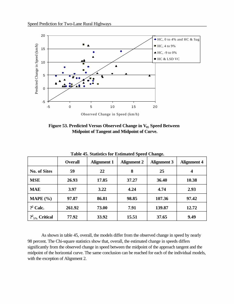
Speed Prediction for Two-Lane Rural Highways
-5
0
5
10
15
20
-5 0 5 10 15 20
Observed Change in Speed (km/h)
Pred
icte
d C
hang
e in
Spe
ed (k
m/h
)HC, 0 to 4% and HC & Sag
HC, 4 to 9%
HC, -9 to 0%
HC & LSD VC
Figure 53. Predicted Versus Observed Change in V85 Speed Between Midpoint of Tangent and Midpoint of Curve.
Table 45. Statistics for Estimated Speed Change.
Overall Alignment 1 Alignment 2 Alignment 3 Alignment 4
No. of Sites 59 22 8 25 4
MSE 26.93 17.85 37.27 36.40 10.38
MAE 3.97 3.22 4.24 4.74 2.93
MAPE (%) 97.87 86.81 98.85 107.36 97.42
?2 Calc. 261.92 73.00 7.91 139.87 12.72
?25% Critical 77.92 33.92 15.51 37.65 9.49
As shown in table 45, overall, the models differ from the observed change in speed by nearly98 percent. The Chi-square statistics show that, overall, the estimated change in speeds differssignificantly from the observed change in speed between the midpoint of the approach tangent and themidpoint of the horizontal curve. The same conclusion can be reached for each of the individual models,with the exception of Alignment 2.

Chapter 7. Validation of Speed-Prediction Equations
Box Plots for Speed-Change Estimates
Box plots were developed to illustrate the distribution of the absolute percent difference for thefour speed-prediction models for horizontal curves (Alignments 1 through 4) as well as the difference,absolute difference, and absolute percent difference for the entire validation database. Figure 54includes box plots for the entire data set. These three box plots display the range of error between themodel-predicted change in V85 (i.e., the difference between the V85 at the midpoint of the approachtangent and the V85 at the midpoint of the horizontal curve) and the field-observed change in V85
between these two points.
As can be seen in figure 54, the models were mostly found to overestimate the change in speedbetween the midpoint of the tangent and the midpoint of the horizontal curve. To evaluate each of thefour alignment conditions, box plots were developed for each model, representing the absolute percentdifference between field observations and model-predicted change in V85 between the midpoint of theapproach tangent and the midpoint of the horizontal curve. As can be seen in figure 55, the change inspeed is greatly overestimated for all alignment conditions.

Speed Prediction for Two-Lane Rural Highways
-10
0
10
Diff
eren
ce (k
m/h
)
(a)0
5
10
15
Abs
. Diff
eren
ce
(b)
(km
/h)
0
100
200
300
Ab
s. %
Diff
eren
ce
(c)
Figure 54. Alignment Model Versus Field Observation (All Data).

Chapter 7. Validation of Speed-Prediction Equations
0
100
200
300
Abs
. %
Diff
eren
ce
(a) Model 10
100
200
300
Ab
s. %
Diff
eren
ce
(b) Model 2
0
100
200
300A
bs. %
Diff
eren
ce
(d) Model 40
100
200
300
Abs
. % D
iffer
ence
(c) Model 3
Figure 55. Absolute Percent Difference for Each Alignment Model.

Speed Prediction for Two-Lane Rural Highways
SUMMARY-VALIDATION OF SPEED-PREDICTION EQUATIONS ANDACCELERATION/DECELERATION MODELS
The validation of the six speed-prediction equations for horizontal and vertical curves wasperformed by comparing the equation-predicted V85 at the midpoint of the curve to the field-observedV85 at the midpoint of the curve. The six speed-prediction equations perform well in that they range inmean absolute percent error between 4.1 percent and 10 percent and have an overall mean absolutepercent error of 5.7 percent. Box plots were developed to demonstrate the range in error between theequations and the field measurements as well as displaying any outliers that may be present in the datasets.
A validation was also conducted for the predicted speed change between the midpoint of theapproach tangent and the midpoint of the horizontal curve. In general, the speed changes predicted bythe simplified method used in this chapter were found to differ from the observed changes in speedbetween the tangent and the horizontal curve by an average of 98 percent. As noted previously, thisdifference is not a reflection of the accuracy of the final speed-profile model presented in the followingchapter.

8. DESIGN-CONSISTENCY EVALUATIONS AND SPEED-PROFILE MODEL
SPEED-PREDICTION EQUATIONS USING ALL AVAILABLE DATA
The equations recommended in chapter 3 used 103 of the 176 study sites. The remaining 73sites were selected for validation of the previous research conducted by Krammes et al. and theequations presented in chapter 3.(7) Based on the validation results of chapter 7 and a desire to use allavailable data, a decision was made to use all collected data to generate equations that would be basedon more study sites than any previous efforts. The following sections discuss the new equations.
Horizontal Curves on Grades
Four different vertical grade conditions were considered in the preliminary evaluation ofhorizontal curves on grades: upgrades (0 to 4 percent), steep upgrades (greater than 4 percent),downgrades (-4 to 0 percent), and steep downgrades (less than 4 percent). The data were analyzedbased on these grade separations. A correlation matrix was developed to identify relationships betweenindependent and dependent variables. Based on the correlation matrix and the statistical findings inchapter 3, the independent variables evaluated in the regression analysis were radius and inverse radius.Figures 56 and 57 show the data for the 94 sites that had a horizontal curve on a grade. Figure 56shows the speed data versus the radius of the horizontal curve, while figure 57 shows the speed dataversus the inverse radius of the horizontal curve. Both of these figures also include plots of thedeveloped equations.
Figure 56 shows that as R increases from 0 to 400 m, the 85th percentile speeds increasenotably for all study locations. For radii greater than 400 m, the increase in speed is not as dramatic.The inverse of the radius was the variable most highly correlated to the 85th percentile speed of all thevariables included within the correlation matrix. The regression model developed to fit the data forhorizontal curves on grades included the single independent variable 1/R. The plot of 1/R versus 85th
percentile in figure 57 shows a linear relationship with speed.
Table 46 lists the equations developed using all available data. Not unexpectedly, some of theR2 values are lower than for the chapter 3 equations. This could be caused by the greater number ofobservations included for each alignment type. The similarity of the magnitude of the Beta valuesbetween the previous equations and the equations using all data for each alignment condition supportsthe validation process of the chapter 3 equations.
Three of the four revised equations have intercept values greater than the 97.9 km/hrecommended by Krammes et al. on long tangents.(7) Therefore, under certain situations, the equations

Speed Prediction for Two-Lane Rural Highways
would predict speeds higher than the assumed speed on a long tangent. Observed speeds on longtangents ranged from 93 to 104 km/h (average 85th percentile speed by State).
50
60
70
80
90
100
110
0 250 500 750 1000
Radius (m)
85th
Per
cent
ile S
peed
(km
/h)
> 4%
0 to 4%0 to -4%< -4%
Equation for > 4%Equation for 0 to 4%
Equation for 0 to -4%Equation for < -4%
Figure 56. Horizontal Curves on Grades: V85 Versus R.
50
60
70
80
90
100
110
0 0.002 0.004 0.006 0.008 0.01 0.012
1/R
85th
Per
cent
ile S
peed
(km
/h)
> 4%0 to 4%0 to < -4%< -4%Equation for > 4%Equation for 0 to 4%Equation for 0 to -4%Equation for < -4%
Figure 57. Horizontal Curves on Grades: V85 Versus 1/R.

Chapter 8. Design-Consistency Evaluations and Speed-Profile Model
Table 46. Parameter Estimates of Horizontal Curves on Grade.
AlignmentCondition
IndependentVariable
BetaParameterEstimate
p-Value Number R2
0%# G < 4%1/R -3574.51 0.0001
25 0.76Intercept 104.82 0.0001
4%# G < 9%1/R -2752.19 0.0001
23 0.53Intercept 96.61 0.0001
-4%# G < 0%1/R -3709.90 0.0001
25 0.76Intercept 105.98 0.0001
-9%# G < -4% 1/R -3077.13 0.000121 0.58
Intercept 102.10 0.0001
Based on the data and engineering judgment, the maximum operating speed on horizontal curves andtangents could be rounded to 100 km/h. Thus, operating speeds on large-radius horizontal curvesshould be truncated to 100 km/h (or to another desired operating speed) when the predicted speedexceeds this value.
Vertical Curves on Horizontal Tangents
Vertical curves on horizontal tangents were divided into three categories: non-limited sight-distance (NLSD) crest curves, limited sight-distance (LSD) crest curves, and sag curves. A combinedtotal of 21 study sites were collected for the vertical curves on tangents: 2 for NLSD crest curves, 10for LSD crest curves, and 9 for sag curves.
Four different correlation matrices were developed for vertical curves on tangents: individualmatrices containing the data for each vertical curve type and one matrix that combined the NLSD andLSD crest curves. The independent variables considered included K and 1/K. Figure 58 shows the85th percentile speed versus K. Of the independent variables, 1/K was most highly correlated to the85th percentile speeds, even though the correlation was low for some conditions. The relationshipbetween 85th percentile speed and 1/K is shown in figure 59. Also included on these figures are thedata from the NCHRP Stopping Sight Distance (SSD) study and the plot of the selected regressionequation for the limited sight-distance condition.(36)

Speed Prediction for Two-Lane Rural Highways
60
70
80
90
100
110
120
130
0.000 0.020 0.040 0.060 0.080 0.100 0.120Inverse K-Value (1/K)
85th
Per
cent
ile S
peed
(km
/h)
NLSDLSD
SSD Data - NLSD
SSD Data- LSD
Sag
Equation for LSD
Figure 59. Vertical Curves on Horizontal Tangents: V85 Versus 1/K.
60
70
80
90
100
110
120
130
0 50 100 150 200 250K-Value (m/%)
85th
Per
cent
ile S
peed
(km
/h)
NLSD
LSD
SSD Data - NLSD
SSD Data- LSD
Sag
Equation for LSD
Figure 58. Vertical Curves on Horizontal Tangents: V85 Versus K.

Chapter 8. Design-Consistency Evaluations and Speed-Profile Model
Based on the small data set for NLSD vertical curves (only two sites), the data from theNCHRP SSD Study for NLSD curves were added to the correlation matrix.(36) The addition of theSSD study data increased the number of study sites to four data points. Based on the small amount ofdata and the wide variability in speeds observed, no statistically significant regression equation wasfound for NLSD curves on horizontal tangents. Therefore, the desired speed for long tangents isassumed for this condition. This recommendation is based on the graphical representation of the foursites and engineering judgment.
Ten study sites were available from the current study and 32 sites from the SSD study for theevaluation of the LSD sites. The review of the correlation matrix found 1/K to be correlated with the85th percentile speeds. Regression analysis showed that 1/K was significant (0.033); however, the R2
value was extremely low (0.10). A possible reason for the low R2 was that there was a study locationwhere the posted speed was 112.7 km/h, resulting in a large variation in 85th percentile speeds. Whileall the SSD sites had a speed limit of 88.5 km/h, the data were collected prior to the repeal of thenationally mandated speed limit and there was an observable difference in the plot of the data. The SSDspeed data were consistently lower then the speed data observed in the current research. Therefore,the SSD data were not included in the final equation development. The equation was developed fromthe nine observations where the posted speed was less than or equal to 88.5 km/h. The parameterestimates are listed in table 47.
Table 47. Parameter Estimates of LSD Crest Curves on Horizontal Tangents.
Independent Variable
ParameterEstimate P-Value Number
of Sites R2
Intercept 105.08 0.00019 0.60
1/K -149.69 0.0134
A total of nine sag curves on horizontal tangents sites were available for the analysis. As withthe crest curves, the scatter plot does not show a clear relationship between the variables (see figure 58or 59). One possible reason for the poor relationship between 85th percentile speed and K or 1/Kcould be due to the different posted speeds where data were collected. Of the nine sites, two of thesites had posted speeds of 112.7 km/h. A statistical test showed these sites to be data outliers and theywere eliminated from the analysis. An equation was developed for the remaining seven sites. Table 48shows the parameter estimates and statistics of the equation. The R2-value for the equation was 0.49;however, the independent variable, 1/K, was not significant. Therefore, based on the plots and theregression analysis, it is recommended that the desired speed on long tangents be used for thisalignment condition. Extreme sag vertical curves where the K-value is less than 15 may result in

Speed Prediction for Two-Lane Rural Highways
reduced operating speeds; however, the available data are too sparse to make a definitive conclusionon the issue.
Table 48. Parameter Estimates of Sag Curves on Horizontal Tangents.
Independent Variable ParameterEstimate P-Value Number of
Sites R2
Intercept 100.21 0.00017 0.49
1/K -106.34 0.0779
Recommend: Use desired speed on long tangent.
Combination of Horizontal and Vertical Curves
The analysis of the combination curves (i.e., sites with both a horizontal curve and a verticalcurve) began with plotting the speed data versus R, 1/R, K, and 1/K. These plots are shown in figures60, 61, 62, and 63, respectively. Initial evaluation of the plots indicated that both R and K couldinfluence the speed along the combination of curves.
For non-limited sight-distance crest vertical curves in combination with horizontal curves, theefforts discussed in chapter 3 did not find a statistically significant regression equation. One of thereasons was that the data used in the analyses were for larger radii curves. Drivers on a combination oflarge horizontal radii and non-limited sight-distance crest curves may not feel the need to reduce theirspeed in response to the geometry. The inclusion of all available data from this study also did notidentify a regression equation with significant variables. All tested models that used variations of R andK had both insignificant variables and very low R2 values. Therefore, engineering judgment must beused to determine the predicted speed for a horizontal curve combined with a non-limited sight-distancecrest vertical curve. Based on a review of the data available for this condition and for similar conditions,the lowest speed predicted using the equation developed for the following conditions is recommended:
• Assumed maximum desired speed on long tangents.• Predicted speed using the horizontal curve radius equation for the upgrade. • Predicted speed using the horizontal curve radius equation for the downgrade.
Using the lowest predicted speed will ensure that the speed predicted along the combined vertical andhorizontal curve will not be better than if just the horizontal curve was present.
Limited sight-distance crest curves combined with horizontal curves were evaluated using the22 study sites available. Regression analysis compared the influence of 1/K, 1/R, and an interaction

Chapter 8. Design-Consistency Evaluations and Speed-Profile Model
term. The analysis demonstrated that only 1/R was significant in predicting 85th percentile speeds. Table49 lists the parameter estimates for the developed equation.

Speed Prediction for Two-Lane Rural Highways
60
70
80
90
100
110
120
130
0 200 400 600 800 1000 1200Radius (m)
85th
Per
cent
ile S
peed
(km
/h)
Combined NLSDCombined LSDCombined SagEquation for Combined LSDEquation for Combined Sag
Figure 60. Combination Curves: V85 Versus R.
60
70
80
90
100
110
120
130
0.000 0.002 0.004 0.006 0.008 0.010 0.012Inverse Radius (1/R)
85th
Per
cent
ile S
peed
(km
/h)
Combined NLSDCombined LSDCombined SagEquation for Combined LSDEquation for Combined Sag
Figure 61. Combination Curves: V85 Versus 1/R.

Chapter 8. Design-Consistency Evaluations and Speed-Profile Model
60
70
80
90
100
110
120
130
0 50 100 150 200 250K-Value (m/%)
85th
Per
cent
ile S
peed
(km
/h)
Combined NLSD
Combined LSD
Combined Sag
Figure 62. Combination Curves: V85 Versus K.
60
70
80
90
100
110
120
130
0.000 0.050 0.100 0.150 0.200Inverse K-Value (1/K)
85th
Per
cent
ile S
peed
(km
/h)
Combined NLSD
Combined LSD
Combined Sag
Figure 63. Combination Curves: V85 Versus 1/K.

Speed Prediction for Two-Lane Rural Highways
Table 49. Parameter Estimates of CombinedHorizontal and LSD Crest Curves.
IndependentVariable
ParameterEstimate P-Value Number
of Sites R2
Intercept 103.24 0.000122 0.74
1/R -3576.51 0.0001
The revised equation developed for the combination of sag vertical curves and horizontal curveshad an additional nine observations included in the analysis. The equation developed with the data fromthe 25 sites revealed that 1/R was the only significant independent variable. Table 50 lists the equationparameter estimates.
Table 50. Parameter Estimates of Combined Horizontal Sag Curves.
IndependentVariable
ParameterEstimate P-Value Number
of Sites R2
Intercept 105.32 0.000125 0.92
1/R -3438.19 0.0001
Comparison of Regression Equations
The equations using radius were tested to determine if there were differences between theslopes of the regression lines. A t-test and indicator variables were used to check pairs of regressionequations. The regression equation for horizontal curves on grades greater than 4 percent was significantly different from the equations for horizontal curves on a 0- to 4-percent grade,horizontal curves on a 0- to -4-percent grade, and horizontal curves combined with sag curves.Observed speeds for upgrades greater than 4 percent were lower than the speeds for the otherhorizontal curves on grade conditions resulting in an equation that was statistically different from theother equations. This difference is apparent in figure 64. Table 51 lists the results of the statisticalevaluations.

Chapter 8. Design-Consistency Evaluations and Speed-Profile Model
5 0
6 0
7 0
8 0
9 0
1 0 0
1 1 0
0 . 0 0 0 0 . 0 0 2 0 . 0 0 4 0 . 0 0 6 0 . 0 0 8 0 . 0 1 0I n v e r s e R a d i u s ( 1 / R )
85th
Per
cent
ile S
peed
(km
/h)
E q u a t i o n f o r > 4 %
Equa t i on fo r 0 t o 4%
E q u a t i o n f o r 0 t o - 4 %
E q u a t i o n f o r < - 4 %
E q u a t i o n f o r C o m b i n e d L S D
E q u a t i o n f o r C o m b i n e d S a g
Figure 64. Plot of Speed-Prediction Equations Using Radius as a Variable.
Table 51. Comparison of Regression Equations.
Equations Compared Number of Sites p-Value for Indicator Variable
0 to 4 % and > 4 %< -4 % 0 to -4 %Combined SagCombined LSD
4846515047
0.0169*0.85850.70710.34470.2523
> 4 % and < -4 % 0 to -4 %Combined SagCombined LSD
44494845
0.0861 0.0139* 0.0018*0.1002
< -4 % and 0 to -4 %Combined SagCombined LSD
474643
0.74000.40800.5626
0 to - 4 % and Combined SagCombined LSD
4148
0.57770.3921
Combined Sag and Combined LSD 47 0.3775
* Indicates a significant difference.

Speed Prediction for Two-Lane Rural Highways
DESIGN-CONSISTENCY EVALUATION AND SPEED-PROFILE MODEL PROCEDURE
The design-consistency evaluation and the speed-profile model consists of several steps asillustrated in figure 65. The following is a discussion of each of these steps:
1. Select desired speed for the alignment.2. Predict speed for each curve using the developed equations.3. Predict grade-limited speed using the TWOPAS equations.4. Select the lowest speed for each element along the alignment.5. Adjust speeds for acceleration and deceleration.6. Perform design-consistency evaluation.7. Complete the speed profile for the alignment.
Select desiredspeed
Predict speed for each curve
Predict grade-limited speedusing TWOPAS equations
Select lowest speed for each element
Adjust speeds for acceleration and deceleration
Complete Speed Profile
PerformDesign
ConsistencyEvaluation
Figure 65. Design-Consistency Evaluation and Speed-Profile ModelFlow Chart.

Speed Prediction for Two-Lane Rural Highways
Select Desired Speed
The initial step is to select the desired speed along the roadway. Desired speed is the speed thatdrivers select when not constrained by the vertical or horizontal alignment. The desired speed for adriver cannot be measured; however, the speeds observed on a tangent beyond the influence ofhorizontal or vertical alignment can serve as an assumed desired speed. Based on the findings reportedin chapter 4, the average 85th percentile speeds on long tangents range between 93 and 104 km/h forthe different States in this study. Therefore, a speed of 100 km/h is a good estimate of the desiredspeed along a two-lane rural roadway when seeking a representative, rounded speed. The long tangentis defined as a tangent that is long enough for a driver to accelerate to and maintain a desired speed forsome distance.
Predict Speed for Each Curve Using the Developed Equations
Several equations were developed to predict speeds for different alignment conditions in thisstudy. Figure 66 illustrates the basic logic for using the speed-prediction equations listed in table 52.The characteristics of the roadway needed for use with the speed-prediction equations are listed at thetop of figure 66 and include the beginning and ending points of the curves, the radius of the horizontalcurve, the vertical grade, and/or the K-value for the vertical curve. This information determines which ofthe three major categories to use: horizontal curve, vertical curve, or tangent section (i.e., no horizontalor vertical curve).
The speeds predicted from the equations represent the speeds measured at the midpoint of thecurve. The model currently assumes that this speed is constant throughout the horizontal or verticalcurve; however, as the data in chapter 6 illustrate, speeds vary throughout the curve. Because a definedpattern of how speed varies through the curve was not present for the 21 horizontal curves (see tables40 and 41), the previous assumption of constant speed for the entire horizontal curve was retained.
Predict Grade-Limited Speed Using the TWOPAS Vehicle Performance Equations
The TWOPAS equations can be used to check the performance-limited speed at every pointon the roadway (upgrade, downgrade, or level). If, at any point, the grade-limited speed is less than thetangent or curve speed predicted using the speed-prediction equations or the assumed desired speed,then the grade-limited speed will govern. Chapter 5 presents the TWOPAS equations and examples ofthe effects of grade on passenger cars and trucks.

Chapter 8. Design-Consistency Evaluations and Speed-Profile Model
S
ag
Eqn
. 8
NL
SD
Eqn
. 9
LSD
Eqn
. 10
Feat
ure
Typ
e
Hor
izon
tal C
urve
On
Gra
de
Ver
tical
Cur
ve
-9 to
-4 %
Eqn.
1
0 to
4 %
Eqn
. 3
4 to
9 %
Eqn.
4
Sag
Eqn.
5
NLS
D
Eqn.
6
Des
ired
Spe
ed
Ver
tical
Cur
veN
o H
C o
r VC
V85
on
HC
V85
on
VC
PT o
f Pre
viou
sC
urve
PC o
f Cur
veR
adiu
sG
rade
VPT
of P
revi
ous
Cur
veV
PC o
f Cur
veK
, App
roac
h G
rade
, Dep
artu
re G
rade
Des
ired
Spee
d
Req
uire
d:
V85
on
Tan
gent
-4 to
0 %
Eqn.
2
LSD
Eqn
. 7
If V
85 >
Des
ired
Spe
ed
T
hen
V
85 =
Des
ired
Spee
d
Not
e: A
lignm
ent-C
ondi
tion
Equa
tions
are
list
ed in
tabl
e 52
.
Figu
re 6
6. S
peed
-Pre
dict
ion
Equ
atio
ns.

Speed Prediction for Two-Lane Rural Highways
Table 52. Speed-Prediction Equations for Passenger Vehicles.AC EQNo. (1) Alignment Condition Equation (2) No. of
Obser.R2 MSE
1.Horizontal Curve on Grade:
-9% # G < -4%21 0.58 51.95V85 ' 102.10 & 3077.13
R
2.Horizontal Curve on Grade:
-4% # G < 0%25 0.76 28.46V85 ' 105.98 & 3709.90
R
3.Horizontal Curve on Grade:
0% # G < 4%25 0.76 24.34V85 ' 104.82 & 3574.51
R
4.Horizontal Curve on Grade:
4% # G < 9%23 0.53 52.54V85 ' 96.61 & 2752.19
R
5.Horizontal Curve Combined With Sag
Vertical Curve25 0.92 10.47V85 ' 105.32 & 3438.19
R
6.Horizontal Curve Combined With
Non-Limited Sight-Distance Crest Vertical Curve
(see note 3) 13 n/a n/a
7.
Horizontal Curve Combined WithLimited Sight-Distance Crest Vertical
Curve (i.e., K # 43 m/%)
V85 ' 103.24 & 3576.51R
(see note 4)
22 0.74 20.06
8.Sag Vertical Curve on Horizontal
TangentV85 = assumed desired
speed7 n/a n/a
9.Vertical Crest Curve With Non-Limited
Sight Distance (i.e., K > 43 m/%) onHorizontal Tangent
V85 = assumed desiredspeed
6 n/a n/a
10.Vertical Crest Curve With Limited Sight
Distance (i.e., K # 43 m/%) on Horizontal Tangent
9 0.60 31.10V85 ' 105.08 & 149.69K

Chapter 8. Design-Consistency Evaluations and Speed-Profile Model
VV
V
V
V
V
V
V
VV
X X
XX
X L S C > L S Ca c
L S C aL S C = Xa c d
L S C > X + XL S C < X + X a n d L S C > X
L S C = X
aa a c d
a
f af a
c d
f df d f sf s
f s
n
n
a
aV n
n + 1
n + 1n + 1
f s f d
c dt d
f a8 5 t h P e r c e n t i le S p e e d8 5 t h P e r c e n t i le S p e e d
8 5 t h P e r c e n t i le S p e e d
D is t a n c e
D is t a n c eD is t a n c e
B e g in o fC u r v e n + 1
B e g in o fC u rv e n + 1B e g in o fC u r v e n + 1
E n d o fC u rv e n
E n d o fC u r v e nE n d o fC u r v e n
AA c c e l e r a t i o n / D e c e l e r a t i o n C o n d i t i o n sB
C
NOTES:1. AC EQ No. = Alignment Condition Equation Number2. Where: V85 = 85th percentile speed of passenger cars (km/h) K = rate of vertical curvature
R = radius of curvature (m) G = grade (%)3. Use lowest speed of the speeds predicted from AC EQ No. 1 or 2 (for the downgrade) and AC EQ No. 3 or 4
(for the upgrade).4. In addition, check the speeds predicted from AC EQ No. 1 or 2 (for the downgrade) and AC EQ No. 3 or 4
(for the upgrade) and use the lowest speed. This will ensure that the speed predicted along the combinedcurve will not be better than if just the horizontal curve was present (i.e., that the inclusion of a limited sight-distance crest vertical curve results in a higher speed).
Select the Lowest Speed for Each Element
The speeds predicted from the previous three methods (assumed desired speed, speedspredicted using the speed-prediction equations, and the speeds from the TWOPAS equations) arecompared and the lowest speed is selected. The speeds for the different alignment features could thenbe compared to identify unacceptable changes in speed between alignment features. For example, adesign-consistency evaluation could be conducted and a flag raised if the speed change from one curveto another is greater than a pre-set number. If a continuous speed profile for the alignment is desired orif the deceleration or acceleration from one curve to another needs to be checked, these lowest speedswould then be used in the following step.
Adjust Speeds for Acceleration and Deceleration
The next step of the design-consistency evaluation is to compare the calculated decelerationand acceleration rates using the lowest speeds determined in the previous step with the recommendedrates present in table 53. In developing a speed-profile model, the next step of the process is toadjusted the speed prior to and departing from a curve. If the speed on a curve is less than the desiredspeed, the driver decelerates when approaching the curve and then accelerates after departing thecurve. Table 53 lists the values determined from either the studies conducted as part of this research(see chapter 6) or the values selected based on engineering judgment and previous research.
The values selected for the speed-profile model are based on the observed speeds at the 21horizontal curves studied in this project (see chapter 6). Three sets of acceleration and decelerationvalues were identified for the design-consistency checks. The range for the initial set, called gooddesign, was selected as being between those observed at the 21 horizontal curves (see chapter 6) andthe value for normal acceleration or deceleration for speed changes between 50 and 60 mph (80.5 and96.6 km/h) as presented in ITE’s Transportation and Traffic Engineering Handbook.(69) The fairdesign range for acceleration was from the normal acceleration rate to the maximum accelerationrate.(69) For deceleration, ITE’s Handbook has a reasonable comfortable rate of 2.46 m/s2; however,only approximately 90 percent of wet pavements provide that level of friction (see figure III-1, part B inAASHTO’s A Policy on Geometric Design of Highways and Streets).(2) To include consideration

Speed Prediction for Two-Lane Rural Highways
for wet pavements, the recommendation is that the fair design range for deceleration be betweennormal deceleration and 2.00 m/s2. Poor design for deceleration would exceed the 2.00-m/s2 valueand for acceleration, it would exceed 1.25 m/s2.
Figure 67 illustrates the different conditions that can occur when evaluating and/or predictingacceleration and deceleration speeds. Six conditions were identified. Supporting equations for theseconditions are listed in table 54.

Chapter 8. Design-Consistency Evaluations and Speed-Profile Model
Table 53. Deceleration and Acceleration Rates.
Deceleration Rate, d (m/s2) Alignment Condition AccelerationRate, a (m/s2)
Speed Profile
Radius, R (m)
R $ 436
d
0.00
1-4 Horizontal Curves on Grade: -9% # G < 9%
Radius, R (m) a
R > 875 0.00
175 # R < 436
R < 175
*% 0.6794 & 295.14R
*
1.00
436 < R # 875 0.21
250 < R # 436 0.43
175 < R # 250 0.54
1.00 5Horizontal Curve Combined
With Sag Vertical Curve0.54
(use rates for Alignment Conditions1 through 4)
6Horizontal Curve Combined
With Non-Limited Sight-Distance Vertical Curve
(use rates forAlignment Conditions
1 through 4)
1.00 7
Horizontal Curve CombinedWith Limited Sight-Distance
Crest Vertical Curve(i.e., K # 43 m/%)
0.54
n/a 8Sag Vertical Curve
on Horizontal Tangentn/a
n/a 9Vertical Crest Curve With Non-Limited Sight Distance (i.e., K >43 m/%) on Horizontal Tangent
n/a
1.00 10
Vertical Crest Curve WithLimited Sight Distance
(i.e., K # 43 m/%) on HorizontalTangent
0.54
where: K = rate of vertical curvature, G = grade (%)
Design Consistency (All Alignment Conditions)
1.00 to 1.48 Good Design 0.54 to 0.89
1.48 to 2.00 Fair Design 0.89 to 1.25
>2.00 Poor Design >1.25

Chapter 8. Design-Consistency Evaluations and Speed-Profile Model
Figure 67. Acceleration/Deceleration Conditions.(See table 54 for variable definitions.)

Speed Prediction for Two-Lane Rural Highways
Figure 67. Acceleration/Deceleration Conditions (continued).
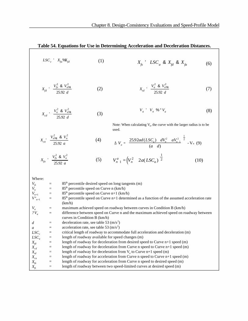
Chapter 8. Design-Consistency Evaluations and Speed-Profile Model
Xfd 'V 2
fs & V 2n%1
25.92 d(2)
LSC c ' Xfa%Xfd (1) Xfs ' LSCa & Xfd & X fa (6)
Xtd 'V 2
a & V 2n%1
25.92 d(7)
Xcd 'V 2
n & V 2n%1
25.92 d(3)
Xca'V 2
n%1 & V 2n
25.92 a(4)
Xfa 'V 2
fs & V 2n
25.92 a(5)
Va ' Vn % ªVa (8)
Table 54. Equations for Use in Determining Acceleration and Deceleration Distances.
Note: When calculating Va, the curve with the larger radius is to beused.
- V (9)∆ Vad LSC dV aV
a daa n n
n=+ +
+
+2592 2
12
12. ( )
( )
( )V V a LSCna
n a+ = +12 2 ( )
12 (10)
Where:Vfs = 85th percentile desired speed on long tangents (m)Vn = 85th percentile speed on Curve n (km/h)Vn+1 = 85th percentile speed on Curve n+1 (km/h)V a
n+1 = 85th percentile speed on Curve n+1 determined as a function of the assumed acceleration rate(km/h)
Va = maximum achieved speed on roadway between curves in Condition B (km/h)?Va = difference between speed on Curve n and the maximum achieved speed on roadway between
curves in Condition B (km/h)d = deceleration rate, see table 53 (m/s2)a = acceleration rate, see table 53 (m/s2)LSCc = critical length of roadway to accommodate full acceleration and deceleration (m)LSCa = length of roadway available for speed changes (m)Xfd = length of roadway for deceleration from desired speed to Curve n+1 speed (m)Xcd = length of roadway for deceleration from Curve n speed to Curve n+1 speed (m)Xtd = length of roadway for deceleration from Va to Curve n+1 speed (m)Xca = length of roadway for acceleration from Curve n speed to Curve n+1 speed (m)Xfa = length of roadway for acceleration from Curve n speed to desired speed (m)Xfs = length of roadway between two speed-limited curves at desired speed (m)

Speed Prediction for Two-Lane Rural Highways
In the previous study, the tangent between horizontal curves was the length of roadway used foracceleration from a curve and deceleration into a curve. If the tangent was sufficiently long, then fullacceleration to the desired speed was achieved. When the tangent length was not sufficient for fullacceleration, other assumptions concerning acceleration were made. This study adds the verticalcomponent to the speed-profile model. While horizontal alignment influences speed in most cases whenvertical and horizontal curves overlap, there are cases when the vertical alignment does affect the speedon the horizontal curve. Also, the vertical alignment can affect speed when no horizontal curvature ispresent. Given that vertical alignment is now considered in the process, the terms and processes used indetermining acceleration and deceleration behavior should be modified from the presentation in theprevious study. The following is a summary of the steps needed to determine the acceleration anddeceleration behavior of vehicles before and after speed-limiting curves.
The distance between speed-limiting curves is termed the “length of roadway available forspeed changes.” This length may be the distance between the end of one horizontal curve to thebeginning of the next horizontal curve (i.e., the tangent length from PT to PC), if the two speed-limitingcurves are horizontal curves. When one of the curves is a vertical curve, then the length of roadway forspeed changes will be from the end of the previous curve to the beginning of the following curve. Thesecurves will be called “Curve n” and “Curve n+1" for this procedure.
The procedure begins with the following:
C Calculate length of roadway available for speed changes, LSCa.C Calculate critical length of roadway needed to accommodate full acceleration and
deceleration, LSCc (see AC EQ #1 in table 54).C Calculate length of roadway for deceleration from desired speed to Curve n+1 speed, Xfd
(AC EQ #2 in table 54).C Calculate length of roadway for deceleration from Curve n speed to Curve n+1 speed, Xcd
(AC EQ #3 in table 54).
The determination of the length of roadway available for speed changes (LSCa) is a criticalcomponent in this process. When one grade-limiting curve immediately follows another similar type ofcurve, then the length of roadway available is the horizontal and/or vertical tangent between the curves.The combination of horizontal and vertical alignment changes that approach. Prior to this, the presenceof a vertical curve between two speed-limiting horizontal curves was ignored. In this procedure, onemust determine whether the curve limits the speed and if it does, then it must be considered whendetermining the available length of roadway. In other words, if a crest vertical curve separates twograde-limited curves (say, a short-radius horizontal curve followed by a sag vertical curve), then thelength of roadway along the crest is available for acceleration and deceleration.

Chapter 8. Design-Consistency Evaluations and Speed-Profile Model
The equations for critical length of roadway and deceleration lengths are listed in table 54. Thecalculated values are then compared to determine which condition exists. If the length of roadwayavailable for speed changes is greater than the critical length of roadway (LSCa >LSCc), then fullacceleration and deceleration occurs. When curves are separated by an adequate distance, theacceleration from the initial curve does not affect the deceleration into the following curve. Basically,each curve is beyond the influence of other curves and drivers reach their desired speed on theroadway between curves. This alignment is shown as Condition A in figure 67.
When the length of roadway is not sufficient to allow full acceleration to desired speed (i.e.,LSCa < LSCc), then the length of roadway needed for deceleration (Xfd) is compared to the availablelength (LSCa). If the length needed for deceleration to Curve n+1 from Curve n is less than the availablelength (i.e., LSCa > Xcd), then some acceleration from the previous curve will occur (see Condition B infigure 67 and the equations listed in table 54). When the distance to decelerate from Curve n to Curven+1 is equal to the available distance (i.e., LSCa = Xcd), vehicles will not accelerate upon departingfrom Curve n. They will begin their deceleration for Curve n+1 upon departing Curve n as shown inCondition C in figure 67.
In some cases, the procedure will determine a deceleration distance from Curve n to Curven+1 that is greater than the available distance (i.e., LSCa < Xcd, see Condition D in figure 67). In these situations, the IHSDM could raise a flag indicating to the user that greaterdeceleration than desirable is occurring between two curves (using the values presented in table 53). Note that the deceleration rates for developing a speed-profile model are based on observedbehavior, while the design-consistency values are based on comfortable values or friction values for wetpavement. Drivers will accept higher values in certain situations and they will begin deceleration prior tothe end of a curve and will continue to decelerate into the next curve. While Condition D should bechecked by the user or include additional checks within IHSDM, it may not be as critical as it initiallyappears.
When the speed on Curve n is less than the speed on Curve n+1, the driver will acceleratebetween the two curves. If the distance available for acceleration is longer than the distance calculatedusing the acceleration rates in table 53, then Condition E in figure 67 applies, otherwise Condition Fapplies. Similar to the deceleration Condition D, the occurrence of Condition F should be checked, butit may not be critical. The acceleration rates listed in table 53 for a speed-profile model were for comfortable, observed levels. Drivers may use higheracceleration rates than shown or they will enter curve n+1 at a speed lower than the value calculatedusing the speed-prediction equations. It would be unusual for a driver to accelerate past a comfortablerate just because of the geometrics (see Va
n+1 in figure 67). The speed-profile model should adjust thedownstream speed to match what a driver will reasonably drive rather than assuming a driver willexceed a given acceleration rate to reach the speed predicted by the equations listed in table 52. If

Speed Prediction for Two-Lane Rural Highways
condition F exists, then the speed on curve n+1 should be adjusted to Van+1 (see figure 67 and table
54).
Perform Design-Consistency Evaluation
One use of the predicted speed values is to perform an evaluation of the consistency betweenfeatures. For example, after the speeds are predicted using the equations listed in table 52, thedifference in speed between curves can be calculated. If the speed change is greater than (or equal to)a preset value, such as 15 km/h, a design inconsistency can be flagged. If greater knowledge of thequality of design is desired, then the following scale (as proposed by Lamm et al.) could beconsidered:(70)
Good Design: ÎV85 # 10 km/hFair Design: 20 km/h $ÎV85 $ 10 km/hPoor Design: ÎV85 $ 20 km/h
The design-consistency evaluation can also be performed after all steps shown in figure 65 arecompleted. This evaluation will allow for consideration of the acceleration and deceleration needs.Consideration of acceleration and deceleration can occur in several forms. For example, if the distanceavailable for acceleration or deceleration is less than desirable (e.g., deceleration and accelerationconditions D or F in figure 67 and values exceeding those listed in table 53), a flag could be raisedinforming the user of the situation. To better represent actual operating conditions when this conditionoccurs, however, IHSDM should include other changes. For example, the current assumption is that allacceleration/deceleration occurs on the tangent; however, observed data demonstrate that someacceleration/deceleration occurs within the curve. Acceptable acceleration/deceleration rates may existif some acceleration/deceleration is assumed to occur on the curves.
The IHSDM could also adjust the curve speed from the speed determined in a previous step toa speed determined using the acceleration/deceleration rates presented in table 53. For example, theprogram may want to raise a flag because the predicted speed on curve n was 90 km/h, the speed on curve n+1 was 100 km/h, and these curves are separated by a very shorttangent (which results in an acceleration rate greater than the value present in table 53). If this conditionexisted in the field, a driver would probably begin accelerating from 90 km/h using an acceptableacceleration rate, would traverse curve n+1 at an increasing speed, and may or may not reach the 100-km/h predicted speed within the curve. If these two curves are closely followed by another curve(curve n+2) with a predicted speed of 85 km/h, then the driver may not try to accelerate to 100 km/hon curve n+1, rather the driver would maintain a speed between 90 and 85 km/h on this middle curve.Incorporating this type of check would also serve to verify that a perceived design inconsistency thatwas flagged because the speed differential between two curves was 15 km/h or greater is really apotential design inconsistency. In the example, the difference in predicted speeds for curve n+1 (100

Chapter 8. Design-Consistency Evaluations and Speed-Profile Model
km/h) and curve n+2 (85 km/h) is 15 km/h, which would raise the design inconsistency flag. Whenacceleration and deceleration are considered, the curve n+1 speed is adjusted to a value between 90and 85 km/h and the speed difference between curve n+1 and curve n+2 is now less than the15-km/hlimit.
Complete the Speed Profile for the Alignment
In this step, the speeds determined from the above steps would be plotted to illustrate thespeed along the alignment. This information is shown within the IHSDM to demonstrate to the users thespeed pattern along the alignment.
SPEED-PROFILE EXAMPLE
The following example illustrates how to apply the model to produce a speed profile. Thegeometry for the sample roadway segment is listed in table 55 and includes three horizontal curves andfour vertical curves. The initial step in the procedure is to select a desired operating speed and in thisexample, a value of 100 km/h was assumed. Next, the geometry of the roadway was used in thespeed-prediction equations (see table 52) to determine the speeds for each curve. The geometry wasreviewed to determine which feature influences speed at a given point. For example, at 1.45 km, thesag vertical curve is controlling the speed. After the sag curve ends at 1.63 km, the speed predicted forthe next feature would normally pass to that assumed for tangents; however, it is determined that thenext feature is close and, therefore, acceleration and/or deceleration (A/D) may influence speed andshould be checked. Following the sag curve at 1.70 km is a combined curve that results in equation (7)(see table 52) being used to predict a speed of 94 km/h for the feature.
Once the speeds are predicted using the equations listed in table 52, TWOPAS was used todetermine locations where speeds are affected by vertical grades for a medium-performance passengercar. The results from the assumed desired speed, the speed-prediction equations, and TWOPAS arethen compared, and the lowest predicted speed is chosen for each feature or grade. Figure 63 showsthe alignment, desired speed, and predicted speeds for the example. The lowest speed for each featurein this example was the speed calculated using the speed-prediction equations.
Figure 68 shows the predicted speeds for the alignment, but does not include acceleration ordeceleration from feature to feature. The acceleration/deceleration rates are calculated based on thealignment and the information in table 53. These rates, along with the predicted speeds, are the inputsinto the equations shown in table 54. The equations determine the distance required to decelerate oraccelerate, which is the distance prior to or following a curve where deceleration or acceleration beginsor ends. Figure 69 shows the speed profile for the sample roadway with the adjustments foracceleration/deceleration.

Chapter 8. Design-Consistency Evaluations and Speed-Profile Model
Table 55. Alignment and Results From Speed-Profile Example.Alignment Speed-Profile Results
Dist.(km)
Descrip-tion
Radius(m)
K(m/%)
Length (m)
ApproachGrade(%)
DepartureGrade(%)
ControllingFeature
EquationNo.a
Speed(km/h)
TangentConditionb
0.00 BEGIN TANGENT TAN 100
0.50 PVC 26 210 3 CREST 10 990.71 PVT -5 A/D A/D 99 C0.85 PC 250 HC 1 901.10 PT TANGENT TAN 100
1.45 PVC 18 175 -5 SAG 8 1001.63 PVT 5 A/D A/D 100 A1.70 PC/PVC 400 40 400 5 COMBINED 7 94
2.10 PT/PVT -5 TANGENT TAN 1002.50 PVC 33 200 -5 SAG 8 1002.70 PVT 1 A/D A/D 100 A2.90 PC 275 HC 3 92
3.18 PT TANGENT TAN 1004.00 END TANGENT TAN 100
a Numbers 1 to 10 = Equations are listed in table 52.A/D = Acceleration and/or deceleration may control on this feature and should be checked.TAN = Assumed desired speed for long tangent controls.
b See figure 67 and tables 53 and 54.

Speed Prediction for Two-Lane Rural Highways
Figure 68. Speed Profile and Alignment.
75
80
85
90
95
100
105
110
0.0 0.5 1.0 1.5 2.0 2.5 3.0 3.5 4.0
Distance (km)
Spee
d (k
m/h
)
TWOPAS SpeedPredicted SpeedDesired Speed
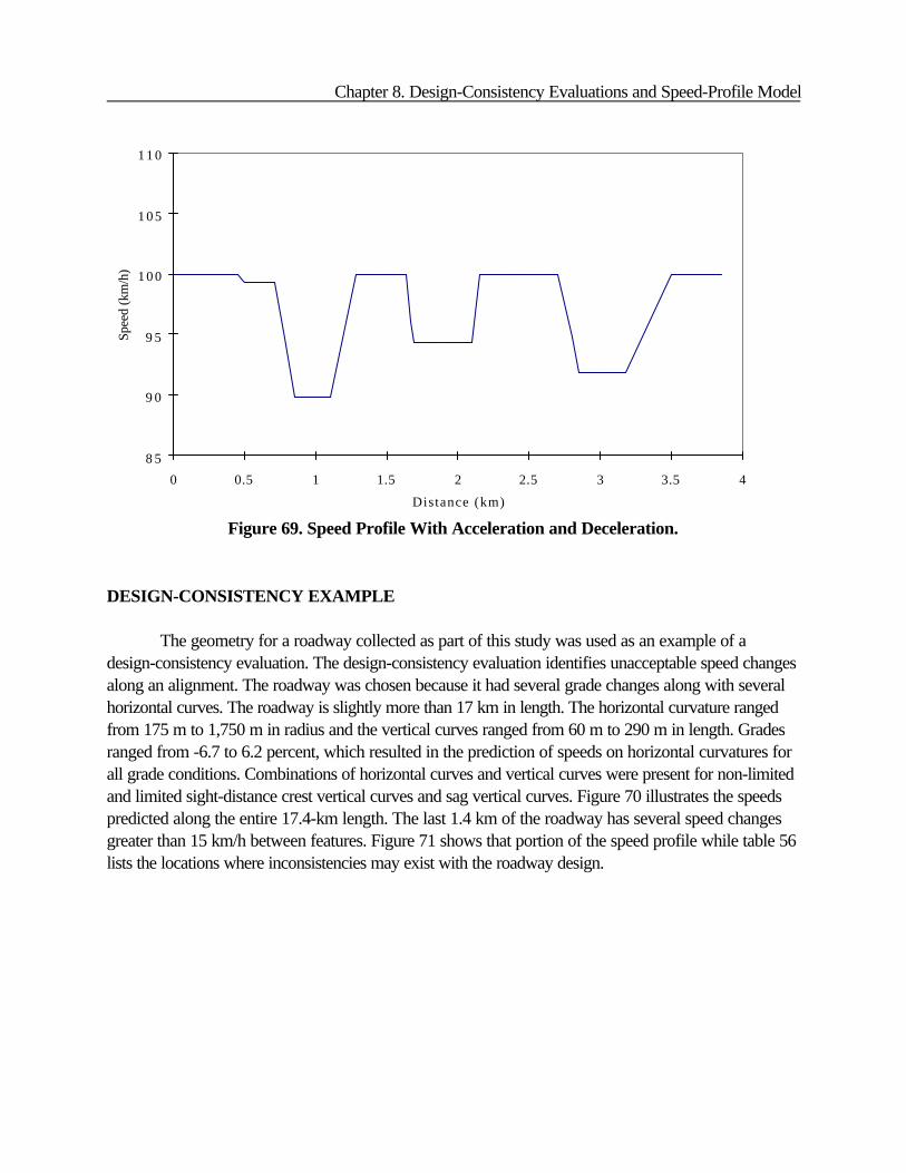
Chapter 8. Design-Consistency Evaluations and Speed-Profile Model
8 5
9 0
9 5
1 0 0
1 0 5
1 1 0
0 0.5 1 1.5 2 2.5 3 3.5 4
Distance (km)
Spee
d (k
m/h
)
Figure 69. Speed Profile With Acceleration and Deceleration.
DESIGN-CONSISTENCY EXAMPLE
The geometry for a roadway collected as part of this study was used as an example of adesign-consistency evaluation. The design-consistency evaluation identifies unacceptable speed changesalong an alignment. The roadway was chosen because it had several grade changes along with severalhorizontal curves. The roadway is slightly more than 17 km in length. The horizontal curvature rangedfrom 175 m to 1,750 m in radius and the vertical curves ranged from 60 m to 290 m in length. Gradesranged from -6.7 to 6.2 percent, which resulted in the prediction of speeds on horizontal curvatures forall grade conditions. Combinations of horizontal curves and vertical curves were present for non-limitedand limited sight-distance crest vertical curves and sag vertical curves. Figure 70 illustrates the speedspredicted along the entire 17.4-km length. The last 1.4 km of the roadway has several speed changesgreater than 15 km/h between features. Figure 71 shows that portion of the speed profile while table 56lists the locations where inconsistencies may exist with the roadway design.

Speed Prediction for Two-Lane Rural Highways
70
75
80
85
90
95
100
105
110
0.0 2.0 4.0 6.0 8.0 10.0 12.0 14.0 16.0 18.0
Distance (km)
Pred
icte
d Sp
eed
(km
/h)
Figure 70. Predicted Speed Profile for Sample Roadway.
70
75
80
85
90
95
100
105
110
16.0 16.2 16.4 16.6 16.8 17.0 17.2 17.4
Dis tance (km)
Pred
icte
d Sp
eed
(km
/h)
P redicted Speeds Using Equations
Design Inconsistency
Figure 71. Closeup of a Portion of the Design-Consistency Evaluation.

Chapter 8. Design-Consistency Evaluations and Speed-Profile Model
Table 56. Location of Design Inconsistency for Sample Roadway.
Location (km) Change in Speed(km/h)
10.7 15
11.0 15
16.4 15
16.6 16
17.1 16
SPEED-PROFILE MODEL ASSUMPTIONS
The speed-profile model developed in this project is to predict the speeds along a continuousalignment using both the vertical and horizontal geometry. The research approach employed to developthe model used either isolated horizontal or vertical curves or, when investigating the horizontal andvertical curve combination, only used curves that overlapped significantly. Data were not collected atsites that did not match the stated criteria. This approach was taken so that a basic understanding couldbe achieved on the relationships between speed and curve geometry. An advantage to the approach isthat we have greater confidence in knowing which elements affect speed along a roadway. Adisadvantage occurs when attempting to determine the changing speed along a complex alignment thatincludes curves that do not fit the criteria developed for the data collection efforts.
The findings from the field-data work were used to develop regression equations to predictspeeds for a given set of conditions. Limitations with regression include using the equation beyond itslimit and the matching of one regression equation to another. For example, questions are raised on thevalidity of the predicted values when the regression equation is used beyond the range of the collecteddata. Another concern is how well regression equations that are developed with different sets of datainteract. For example, in this study, we developed speed-prediction equations based on data collectedalong a set of horizontal curves. We then modified that predicted speed for acceleration anddeceleration performance using a regression equation that was developed from other data. In general,the equations fit well, however, there are cases when adjustments will need to be made because ofthese issues. The following is a discussion on some of the situations identified during the modeldevelopment that need to be considered in using the speed-profile model.
Vertical Curve Type . Vertical curves are categorized into four types. Type I consists ofcurves that have an initial upgrade followed by a downgrade. Type III curves have a downgrade that is

Speed Prediction for Two-Lane Rural Highways
followed by an upgrade. Type I curves are generally viewed as being the “typical” crest vertical curves,while Type III curves are the typical sag vertical curves. Type II curves are also crest vertical curves;however, they are an upgrade followed by a less step upgrade or a downgrade followed by a steeperdowngrade. Type IV curves are sag curves with an upgrade followed by a steeper upgrade or adowngrade followed by a less steep downgrade. This study only collected data at Type I and Type IIIcurves. Therefore, an assumption was made during the model development that all crest curves have asimilar speed relationship as the Type I curves, and that all sag curves have a similar speed relationshipas found for Type III curves.
Speed on Tangent. The previous study suggested that the tangent speed should be assumed tobe 97.9 km/h.(7) This research supported that value and also demonstrated that higher speeds may beobserved on tangents. The desired speed on roadway value was rounded to 100 km/h for use in theexamples.
Maximum Speed on Curves. In some situations, the speeds predicted using the regressionequation are higher than the assumed speed on the tangent. For consistency within the speed-profilemodel, the maximum speed on a curve should be set to the desired speed on the tangent. In theexamples, this speed is 100 km/h. Figure 72 illustrates the plots that would have resulted for the speed-profile example if different desired speeds would have been selected.

Chapter 8. Design-Consistency Evaluations and Speed-Profile Model
75
80
85
90
95
100
105
110
115
120
0 0.5 1 1.5 2 2.5 3 3.5 4
Distance (km)
Spee
d (k
m/h
)
Desired Speed = 110Desired Speed = 105Desired Speed = 100Desired Speed = 95Desired Speed = 90
Figure 72. Effect of Different Assumed Desired Speeds onSpeed-Profile Example.
Minimum Speed on Curves. The smallest radius in the field data set was 100 m. Duringtesting of the model, smaller radii were used to determine how the model would perform. In somecases, the model predicted not only very low speeds, but negative speeds. This is a consequence ofusing a regression equation beyond its limit. To result in a more realistic speed prediction, the minimumpredicted speed is set to 60 km/h when the radius of a horizontal curve is less than 100 m.
Length of Roadway Available for Speed Changes, Formerly Known as TangentLength. Tangent length is a critical portion of an accurate speed-profile model because it is the areawhere all acceleration and/or deceleration is assumed to occur for a curve. In the previous work, thislength was assumed to be from the PT of the previous horizontal curve to the PC of the followinghorizontal curve.(7) Vertical alignment was ignored. This research study was to produce a speed-profilemodel that includes both vertical alignment and horizontal alignment. Given that, one could assume thatthe length is from the end of a curve to the beginning of the next curve, regardless of whether the curveis a vertical curve or a horizontal curve. The findings to date demonstrate that the speed on a non-limited sight-distance crest curve and on sag curves is not influenced by the characteristics of the
vertical curve. Therefore, the determination of the roadway length available for speed changes shouldinclude vertical curves of those types.

Speed Prediction for Two-Lane Rural Highways
Acceleration/Deceleration Rates for Vertical and Vertical/Horizontal Alignment. Themodels developed to predict acceleration and deceleration rates were based on data collected athorizontal curves. Thus, no data were available to predict acceleration/deceleration rates for verticalalignment or for combinations of horizontal/vertical alignment. In these cases, the maximum valuesselected for the sites studied in the project were assumed. In the cases of crest vertical curves withlimited sight distance, the acceleration rate for the departure tangent can be applied starting from theVPI, rather than the VPT, because there the constraint imposed on the driver is removed and the drivercan begin accelerating at that point.
Maximum Acceleration/Deceleration Rates. The models developed provide a maximumacceleration rate of 0.54 m/s2; however, the maximum acceleration observed in the field reached 1.77m/s2. The maximum deceleration rate provided by the models is 1.0 m/s2, while the maximum observeddeceleration rate was 1.44 m/s2. Thus, higher values of acceleration/deceleration may be observed inthe field and are recommended for the design-consistency evaluation.
Acceleration/Deceleration Rates Greater Than Assumed Values. In some situations, thelength available for speed changes is insufficient for the acceleration or deceleration rates listed in table53. There are two possible reasons for this discrepancy: (1) the acceleration/ deceleration modelsdeveloped were based on sites with long approach tangents and horizontal curves only, thus, driversmay apply higher decelerations for more restrictive alignments; and (2) field data showed that there isacceleration and deceleration occurring within the limits of the curve, while the speed-profile modelassumes that all acceleration and deceleration takes place prior or after the horizontal curve.
Overlapping Curves. The speed-profile model is based on the first feature encountered. Thus,if a long horizontal curve is combined with a vertical curve, and the vertical curve begins after the PCand ends before the PT, three predicted speeds will result based on that alignment configuration. Thespeed-profile model examines each feature independently and predicts speeds for the approach grade,the combined curves, and the departure grade based on the horizontal curve radius. If speeds onhorizontal curves are constant throughout the curve, then a method must be incorporated into the speedprofile to check for potential inconsistencies such as the previous example.
A suggested method is to assume that the lowest speed predicted for any condition controlsthroughout the horizontal curve. The speed-profile model would need to check each speed predictedwithin the limits of the horizontal curve to determine the lowest speed. All predicted speeds within thehorizontal curve would then be set to the lower values. Currently, this method is not included in thespeed-profile model because while the method is logical, it may not reflect observed speeds.

9. RELATIONSHIPS OF GEOMETRIC DESIGN-CONSISTENCY MEASURES TO SAFETY
The preceding chapters of this report have developed several geometric design-consistencymeasures of potential value to highway designers in assessing the quality of the horizontal and verticalalignment in the designs they develop. These measures include speed reduction, as determined with thespeed-prediction equations in table 52, and four of the alignment indices presented in table 19.
These geometric design-consistency measures are conceptually attractive and have beencalibrated with actual speed data. However, before a design-consistency methodology is recommendedto geometric designers, it would be valuable to demonstrate that the proposed design-consistencymeasures are, in fact, related to safety. Such a demonstration is presented in this chapter.
The chapter is organized into four major sections. The first section describes the databasedevelopment and analysis methodology. The second section presents the analysis of speed reduction asa design-consistency criterion for horizontal curves. The third section presents the analysis of roadwayalignment indices as design-consistency criteria. The fourth section summarizes the analysis results andpresents the conclusions of the chapter.
ANALYSIS METHODOLOGY/DATABASE DEVELOPMENT
The design-consistency methodology using speed reduction as a measure of geometric designconsistency is based on a series of speed-prediction models developed through regression analysis. The10 speed-prediction equations representing the effects of motorist speeds on both horizontal andvertical alignment have been presented in table 52. Taken together, these models allow the prediction ofspeeds for the sequence of individual features along a two-lane rural highway accounting for the effectsof horizontal and vertical alignment. In particular, the models can be used to evaluate the speedreductions between successive tangents and horizontal curves and between successive (i.e., back-to-back) curves.
Databases were developed to test the relationship to safety of the speed-reduction measure andto evaluate the relationship to safety of the roadway alignment indices. To assemble these databases,data were obtained from the FHWA Highway Safety Information System (HSIS) for State-maintained,two-lane rural highways in Washington State. These databases are clearly representative data setsbecause they include all two-lane rural highways under State jurisdiction in Washington, not just asample. The Washington HSIS data included roadway inventories, traffic volume, horizontal alignment,vertical alignment, and accidents for 3 years (1993-1995).

Speed Prediction for Two-Lane Rural Highways
Selection of Analysis Sites
Because the available database was so comprehensive, a careful review was required to selectsections that were suitable for analysis. A minimum section length of 6.4 km and a maximum sectionlength of 32 km were established for this analysis. These minimum and maximum section lengths wereprimarily intended to make the database appropriate for the analysis of roadway alignment indices.Sections shorter than 6.4 km might not provide enough individual geometric features to compute arepresentative value of the alignment indices. Sections longer than 32 km might be so varied that nosingle value of an alignment index would be representative of the section as a whole (i.e., there is astrong likelihood that any longer section would be non-homogeneous). Following this process, 291highway sections, with a total length of 4,930 km, were available for analysis.
The first step was to review the data for each route and eliminate portions of the roadway withfeatures that might interfere with the analysis. The following types of locations were eliminated fromconsideration:
• All locations within 0.8 km of an intersection, with STOP or signal control for traffic on themajor road (i.e., the State highway) or within 0.8 km of ramps at freeway-arterial orarterial-arterial interchanges.
• All locations within 0.8 km of a tunnel or a railroad grade-crossing.
• All locations within small towns with speed limits less than 80 km/h, including a buffer areaof 0.4 km at either end of the reduced-speed zone.
• All locations within a passing or climbing lane, including a buffer area of 0.4 km at eitherend of the passing or climbing lane.
Sections were also subdivided at intersections with major changes in average daily traffic (ADT). Theremaining sections that were less than 6.4 km in length were then discarded and roadway sections morethan 32 km in length were subdivided.
Roadway and Traffic Data
Roadway inventory and traffic data were obtained from the HSIS files for each of thesesegments. All of the segments analyzed had posted speed limits of 88.5 km/h or more. The trafficvolumes of the study sections ranged from 200 to 18,000 veh/day.
Alignment Data
The Washington HSIS files contain data on the geometrics of each horizontal and vertical curve

Chapter 9. Relationships of Geometric Design-Consistency Measures to Safety
on the highway. For horizontal curves, these data included the location of the point of curvature (PC),the location of the point of tangency (PT), and the radius and length of the curve. For vertical curves,the available data included the approach grade, the departure grade, the algebraic difference in grade, and the length of the curve. The locations of the geometric features weregiven in the same milepost system used to specify accident locations.
The 291 highway sections were subdivided into individual horizontal curves and tangents andthe vertical alignment of each tangent and curve was determined. The predicted 85th percentile speed ofmotorists on each tangent and curve was determined using the speed-profile models in table 52 and thespeed differences between successive features (i.e., tangent/curve, curve/tangent, or curve/curve) weredetermined. These speed differences generally represented a speed reduction in one direction of traveland a speed increase in the other.
The final database included 5,287 horizontal curves for which the speed differences fromadjacent features could be determined.
The alignment data were also used to compute various alignment indices that are discussed laterin this chapter.
Accident Data
The accident data from the HSIS files were used to determine the 3-year accident experienceof each individual tangent and horizontal curve. The accident analysis considered only non-intersectionaccidents that involved: (1) a single vehicle running off the road; (2) a multiple-vehicle collision betweenvehicles traveling in opposite directions; or (3) a multiple-vehicle collision between vehicles traveling inthe same direction. These are the same accident types that Zegeer et al. have identified as being “over-represented on curves as compared to tangents.”(70) All accidents involving parking, turning, or passingmaneuvers; animals in the roadway; or bicycles or motorcycles were excluded.
ANALYSIS OF SPEED REDUCTION AS A DESIGN-CONSISTENCY CRITERION FOR HORIZONTAL CURVES
General Relationship Between Quality of Horizontal Curve Design and Safety
Several guidelines have been recommended for maximum speed reductions from tangents tohorizontal curves and for maximum differentials between design and operating speeds on horizontalcurves. Lamm et al. suggest that the ranges shown in table 57 represent good, fair, and poor designwith respect to the differences among the 85th percentile operating speeds on successive alignmentfeatures.(15)

Speed Prediction for Two-Lane Rural Highways
As a first test of the speed-reduction criterion proposed as a measure of design consistency,5,287 individual horizontal curves from the roadway sections in Washington were classified as good,fair, and poor with respect to design safety using the criteria in table 57. This included all horizontalcurves for which the speed reduction for both directions of travel fell in the same design safety level asdefined by Lamm et al.(15) Table 58 presents a summary of the accident frequencies, exposure, vehicle-kilometers of travel, and accident rates for these 5,287 curves.
The average accident rate is highest for the horizontal curves in the poor category and lowestfor the horizontal curves in the good category. These results provide a first indication that horizontalcurves that require motorists to make greater speed reductions from the approach tangent are likely tohave higher accident rates than horizontal curves requiring lower speed reductions.
Table 57. Design Safety Levels Proposed by Lamm et al. (15)
Design Safety Level
Good Fair Poor
ªV85 # 10 km/h 10 km/h < ªV85 # 20 km/h ªV85 > 20 km/h
ªV85 = difference in 85th percentile speed between successive geometric elements(km/h).
Table 58. Accident Rates at Horizontal Curves by Design Safety Level.
DesignSafety Level
Number ofHorizontal
Curves
3-YearAccident
FrequencyExposure
(million veh-km)
Accident Rate(accidents/
million veh-km)GoodFairPoor
4,518 622 147
1,48321747
3,206.06150.4617.05
0.461.442.76
Combined 5,287 1,747 3,373.57 0.52
Explicit Relationship Between Speed Reduction and Accidents at Horizontal Curves
The initial analysis showed that the quality of design of a horizontal curve does appear to berelated to safety. Therefore, an explicit quantitative relationship between speed reduction and safetywas developed to test its appropriateness as a design-consistency measure.
The 5,287 curves experienced a total of 1,747 accidents over the 3-year period from 1993 to1995, with a mean of 0.11 accidents per curve per year. However, a large proportion of the curves

Chapter 9. Relationships of Geometric Design-Consistency Measures to Safety
(93.2 percent) experienced one or no accident during the 3-year period. The distribution of theseaccidents is shown in table 59 and figure 73.

Speed Prediction for Two-Lane Rural Highways
0%
20%
40%
60%
80%
100%
4,152
775
21584 35 13 10 2 1
Number of accidents in 3 years
Per
cent
of c
urve
s
0 1 2 3 4 5 6 7 8 9 10 11
Table 59. Accident-Frequency Distribution for Horizontal Curves.
Number ofAccidentsin 3 Years
Numberof Curves
Percentageof Curves
01234567
11
4,1527752158435131021
78.53 14.664.071.590.660.250.190.040.02
Figure 73. Accident-Frequency Distribution at Horizontal Curves.

Chapter 9. Relationships of Geometric Design-Consistency Measures to Safety
Using loglinear regression models, the relationship between accident frequencies and exposure,curve geometries, and speed-reduction variables was investigated. Based on the shape of the accidentdistribution, it was decided to use Poisson and negative binomial regression models. This approach hasbeen successfully used previously.(71) The Poisson distribution is an appropriate choice since accidentfrequencies are: (1) integers, (2) relatively small numbers, and (3) necessarily non-negative. However, abasic assumption underlying the use of the Poisson distribution is that its mean and variance are equal.This assumption is not always the case. When this assumption is substantially violated (for example, ifthe distribution has a long tail), then the negative binomial (NB) distribution can provide an improvementover the Poisson distribution. This distribution is chosen whenever the data exhibit either extra variation(overdispersion) or too little variation (underdispersion) relative to that assumed by the Poissondistribution.
The functional relationship between accident frequencies and selected (independent) variableswas investigated. The following variables were included in the Poisson models:
• AADT (veh/day).• Horizontal curve length (km).• Curve radius (m).• Speed reduction (km/h).
Two approaches were used to treat exposure. First, annual average daily traffic (AADT) andcurve length were both included in the model and their coefficients in the regression model wereestimated separately. In this approach, the natural logarithm of AADT and curve length, rather thantheir untransformed values, were used in modeling. This same approach has been taken by otherresearchers where accident counts rather than accidents rates are modeled.
The second approach was to combine AADT and curve length into million vehicle-kilometersof travel, a common exposure measure for roadway sections. In this approach, the exposure measurewas used in the analysis simply as a scale factor (i.e., its coefficient in the model was forced to be equalto 1.0).
Basic statistics for the independent variables included in the models are shown in table 60.

Speed Prediction for Two-Lane Rural Highways
Table 60. Descriptive Statistics for 5,287 Horizontal Curves.
Parameter Minimum Mean Median Maximum
Number of accidents in 3 yearsAADT (veh/day)Horizontal curve length (km)Exposure (million veh-km)Horizontal curve radius (m)Speed reduction (km/h)
0222
0.0160.00619.5
0
0.332,2830.2380.638860.83.91
01,5670.1770.321582.60.3
1118,0052.97719.77715,25032.4
The general functional form selected for this analysis was a multiplicative model relating theexpected accident frequencies (Y) at horizontal curves and the independent variables, X1,ÿ, Xn, asfollows:
Y = exp(ß0) exp(ß1X1) exp(ß2X2) ÿ exp(ßnXn) (34)
In the models evaluated here, X1, X2, and X3 represent log(AADT), log(curve length), and speedreduction, respectively. Models of this type were fitted using the GENMOD procedure of the SASstatistical package.(72)
When modeling 3-year accident frequencies as a function of log(AADT), log(curve length), andspeed reduction, the following statistically significant Poisson regression model was obtained:
Y = exp(-7.1977) AADT0.9224 CL0.8419 exp(0.0662 SR) (35)
where: Y = number of accidents that occurred on the horizontal curve during a 3-yearperiod
AADT = annual average daily traffic volume (veh/day)CL = horizontal curve length (km)SR = speed reduction on horizontal curve from adjacent tangent or curve (km/h)
All three parameters were significant at the 95-percent confidence level. In fact, the significancelevels associated with all three parameters were less than 0.0001. In order of importance of theircontribution explaining the variability in the accident data (as measured by their chi-square value), thethree parameters rank as follows: log(AADT) (?2 = 863), log(CL) (?2 = 638), and SR (?2 = 200).
The overall fit of a Poisson (or NB) model can be assessed using the following goodness-of-fitcriteria: the deviance (a measure of over- or underdispersion of the data, which under ideal conditionsshould be close to 1); the Pearson chi-square (another measure similar to the deviance, which shouldalso be close to 1; generally, a value between 0.8 and 1.2 is an indication that the model can beassumed to be appropriate in modeling the data); the ordinary multiple correlation coefficient (R2); and

Chapter 9. Relationships of Geometric Design-Consistency Measures to Safety
the Freeman-Tukey correlation coefficient (R2FT), each correlation with a maximum of 100 percent. A
discussion of these goodness-of-fit parameters can be found in SAS documentation and in Fridstrom etal.(72-73)
The deviance for this Poisson model was 0.830 and its Pearson ?2 was 1.210. Although thesetwo statistics deviate somewhat from 1.0, the Pearson ?2 is just outside the generally acceptable rangeof 0.8 to 1.2, an indication that the model can be considered appropriate in modeling the data. Themodel, however, could not be improved using the NB distribution and this same set of independentvariables. The two correlation coefficients were R2 = 19.5 percent and R2
FT = 17.9 percent, indicatingthat a large proportion in the variation in accident data among the 5,287 curves is not accounted for bythis Poisson model.
A second Poisson model in which exposure, as defined above, was used as a scale factor,rather than AADT and curve length as separate variables, provided the following significant model:
Y = exp(-0.8571) MVKT exp(0.0780 SR) (36)
where: MVKT = exposure (million veh-km of travel for a 3-year period)
The deviance for this Poisson model was 0.836 and its Pearson ?2 was 1.344; the twocorrelation coefficients were R2 = 15.6 percent and R2
FT = 16.8 percent, indicating that this modelexplains slightly less of the variation in accident data than the previous one.
While neither of the models presented in equations 35 and 36 explains a large proportion of thevariation in accident data, this observation is often the case with regression relationships betweengeometric design elements and safety. A key finding is that both models show a strong relationshipbetween the speed reduction on a horizontal curve and the accident frequency on that curve. In bothrelationships, the speed reduction effect is highly significant, since the significance level in both caseswas less than 0.0001. The direction of both relationships indicates that the greater the speed reductionexperienced by motorists on a horizontal curve, the greater its accident experience. Thus, speedreduction appears very promising as a design-consistency measure.
Table 61 presents a sensitivity analysis of the accident-prediction model in equation 36. Thetable shows the sensitivity of predicted accident experience to speed reduction on a horizontal curve.For the typical range of speed reduction shown in the table, the accident rate varies by a factor of 4.0.More specifically, for the middle 50 percent of the speed-reduction range (based on the 25th and 75th
percentiles of speed reduction from the actual Washington alignment data), the accident rate varies by afactor of 1.5. These results indicate that speed reduction not only has a statistically significantrelationship to accident frequency, but that predicted accident frequency varies with speed reduction ina manner that is realistic and is meaningful in engineering terms. Thus, the sensitivity analysis lendssupport to the use of speed reduction as a design-consistency measure.

Speed Prediction for Two-Lane Rural Highways
Table 61. Sensitivity of Safety Measures for Individual Horizontal Curvesto Speed Reduction.
AADT
CurveLength(km)
SpeedReduction
(km/h)
No. of Accidents
in 3 Yearsa
Accident Rate(per million
veh-km)
Accident Rate(per km per
year)2,000 1 2 1.09 0.50 0.362,000 1 5 1.37 0.63 0.462,000 1 10 2.03 0.93 0.682,000 1 20 4.42 2.02 1.475,000 1 2 2.72 0.50 0.915,000 1 5 3.43 0.63 1.145,000 1 10 5.07 0.93 1.695,000 1 20 11.06 2.02 3.69
10,000 1 2 5.43 0.50 1.8110,000 1 5 6.86 0.63 2.2910,000 1 10 10.14 0.93 3.3810,000 1 20 22.11 2.02 7.37
aBased on the model for Speed Reduction shown in equation (36).
Regression models analogous to equations (35) and (36) were developed using radius ofcurvature rather than speed reduction as an independent variable. Radius of curvature was found to bestatistically significant in these models, but predicted accident experience was much less sensitive toradius of curvature than to speed reduction; for curve radius, accident rate changed by a factor of 1.2to 1.3 as curve radius decreased from its 75th to 25th percentile values, as apposed to a factor of 1.5for a similar change in speed reduction. When both speed reduction and radius of curvature were usedas independent variables in the same models, speed reduction was found to have a stronger associationwith accident rate than curve radius (?2 = 190 vs. ?2 = 18). These findings indicate that there is potentialvalue in improving the safety of proposed highway design, through use of a design-consistencyprocedure based on speed reduction, because speed reduction is a better predictor of accidentexperience than curve radius alone.
ANALYSIS OF ROADWAY ALIGNMENT INDICES AS DESIGN-CONSISTENCY CRITERIA
An alternative method for measuring the design consistency of a roadway alignment is withalignment indices (see chapter 4 and a companion report from this research project).(8) Alignmentindices are quantitative measures of the general character of a roadway segment’s alignment. When thegeneral character of an alignment changes between segments of roadway, geometric inconsistencies

Chapter 9. Relationships of Geometric Design-Consistency Measures to Safety
rise. A common example is where the terrain transitions from level to rolling or mountainous, and thealignment correspondingly changes from gentle to more severe.
Proposed indicators of geometric inconsistency include the following:
• Large increase/decrease in the values of alignment indices for successive roadwaysegments.
• High rate of change in alignment indices over some length of roadway.• Large difference between the individual feature and the average value of the alignment
index.
Alignment indices have several advantages for use in design-consistency evaluations. First, theyare easy for designers to use, understand, and explain. Second, alignment indices are a function ofhorizontal and/or vertical alignment elements. Therefore, they provide a mechanism for quantitativelycomparing successive geometric elements from a system-wide perspective, which is the basis of designconsistency. Third, alignment indices can attempt to quantify the interaction between the horizontal andvertical alignments, a design strategy currently missing from design policy. Under AASHTO designguidelines, horizontal and vertical alignments are usually designed separately to meet certain criteria andthen brought together.
The alignment indices proposed as design-consistency measures for entire sections of roadwayinclude: (1) average radius, (2) ratio of maximum radius to minimum radius, (3) average tangent length,and (4) average rate of vertical curvature.(8)
The following discussion addresses the relationship of each of the above alignment indices tothe safety of a roadway section with a length of 6.4 to 32 km (4 to 20 m). A later section of this chapteraddresses the relationship to safety of alignment indices calculated as ratios of an individual feature tothe alignment index for a roadway section. Each of the alignment indices is defined below.
Average Radius
The average radius expresses the sharpness of the curves that motorists typically encounter ona given section of the roadway. A large average radius would indicate curves that are typically not verysharp. Therefore, it is expected that higher speeds would exist for these values compared to smaller

Speed Prediction for Two-Lane Rural Highways
AR ' j Ri
n(37)
RR 'Rmax
Rmin (38)
average radius values. A small average radius indicates that the curves on a roadway section are quitesharp. The average radius for a roadway section is defined as:where: AR = average radius (m)
Ri = radius of ith curve on the roadway section (m)n = number of curves within the section
Maximum Radius/Minimum Radius
The range of the radii along a roadway can be determined by computing the ratio of themaximum to minimum radii. The assumption behind this alignment index is that this ratio can representthe consistency of the design in terms of the use of similar horizontal radii along the road. As this valueapproaches 1 (i.e., as the consistency of the chosen design radii is increased), a reduced accident ratemay be expected. Thus, a section composed of curves of approximately the same radii might beconsidered a consistent design, even if that curve radius was quite sharp, while an otherwise similarsection with a broad range of curve radii might be considered an inconsistent design.
For each roadway section, the ratio of the maximum radius to the minimum radius of theroadway section is computed as:
where: RR = ratio of maximum radius to minimum radiusRmax = maximum radius for any curve on the roadway section (m)Rmin = minimum radius for any curve on the roadway section (m)
While this alignment index appears to be useful, there are three concerns associated with thismeasure. First, if the maximum radius is much different than all other radii, the curve with the maximumradius may be the inconsistency. Second, ratios have different implications for different situations. Forexample, a value of two for this index may be the ratio between either a 1,840-m and 920-m curve or a320-m and 160-m curve. It is likely that motorists would react differently to each situation, therebymaking it difficult to determine inconsistencies. A possible solution to this problem would be to use thisratio together with the average or minimum radius for the roadway section. Third, this alignment index
does not indicate how many curves are being compared, over what length of roadway, and in what
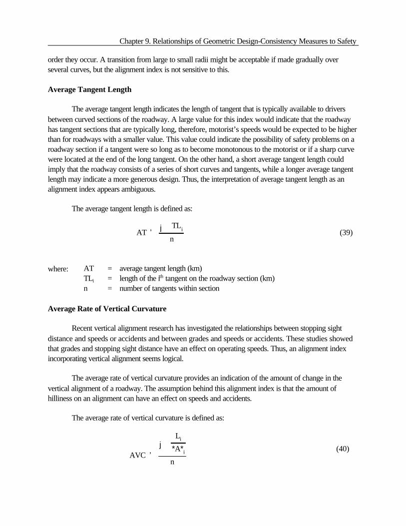
Chapter 9. Relationships of Geometric Design-Consistency Measures to Safety
AT 'j TLi
n(39)
AVC '
jLi
*A*i
n
(40)
order they occur. A transition from large to small radii might be acceptable if made gradually overseveral curves, but the alignment index is not sensitive to this.
Average Tangent Length
The average tangent length indicates the length of tangent that is typically available to driversbetween curved sections of the roadway. A large value for this index would indicate that the roadwayhas tangent sections that are typically long, therefore, motorist’s speeds would be expected to be higherthan for roadways with a smaller value. This value could indicate the possibility of safety problems on aroadway section if a tangent were so long as to become monotonous to the motorist or if a sharp curvewere located at the end of the long tangent. On the other hand, a short average tangent length couldimply that the roadway consists of a series of short curves and tangents, while a longer average tangentlength may indicate a more generous design. Thus, the interpretation of average tangent length as analignment index appears ambiguous.
The average tangent length is defined as:
where: AT = average tangent length (km)TLi = length of the ith tangent on the roadway section (km)n = number of tangents within section
Average Rate of Vertical Curvature
Recent vertical alignment research has investigated the relationships between stopping sightdistance and speeds or accidents and between grades and speeds or accidents. These studies showedthat grades and stopping sight distance have an effect on operating speeds. Thus, an alignment indexincorporating vertical alignment seems logical.
The average rate of vertical curvature provides an indication of the amount of change in thevertical alignment of a roadway. The assumption behind this alignment index is that the amount ofhilliness on an alignment can have an effect on speeds and accidents.
The average rate of vertical curvature is defined as:

Speed Prediction for Two-Lane Rural Highways
where: AVC = average rate of vertical curvature (m/% grade)Li = length of the ith vertical curve on the roadway section (m)|A|i = absolute value of the algebraic difference in grade for the ith vertical curve on
the roadway section (%)n = number of vertical curves within a section
Model Development
Table 62 presents descriptive statistics for the 291 roadway sections evaluated, including the 4alignment indices defined above. The roadway sections include 4,931 km of two-lane rural roadwayswith an average section length of 17 km. A total of 5,824 accidents occurred on these roadwaysections during the 3-year period, ranging from 0 to 42 accidents/year, with an average of 6.7accidents/year.
Figure 74 illustrates the distribution of the accidents on the sections. Only 4.5 percent of theroadway sections (13 out of 291) experienced either zero or one accident during the 3-year period.With this small percentage of sections with low accident frequencies and with a mean accident count of20, the assumption of a Poisson distribution for this distribution would be inappropriate. Figure 74illustrates quite clearly that the shape of the accident distribution is like that of a lognormal distribution;i.e., accident frequencies follow a normal distribution on a logarithmic scale.
Accident frequencies were modeled as a function of exposure (AADT and section length, bothon the logarithmic scale) and each of the four alignment indices—average radius, maximum overminimum radius ratio, average tangent length, and average vertical curvature rate—taken one at a time.The modeling was performed using a standard regression model applied to the log-transformedaccident frequencies. Thus, the general relationship between accident frequencies and exposure anddesign-consistency criterion can be expressed using equation (34), except that the error term of thatmodel has a lognormal rather than a Poisson distribution.

Chapter 9. Relationships of Geometric Design-Consistency Measures to Safety
Table 62. Descriptive Statistics for Roadway Sections.
ParameterNo. of
Sections Minimum Mean Median Maximum
Number of accidents/3 years 291 0 20 15 127
AADT (veh/day) 291 166 2,911 2,061 18,005
Section length (km) 291 6.44 16.95 16.87 32.07
Average radius (m) 282 185 1,099 871 8,591
Maximum radius/minimum radius 282 1.00 13.13 7.92 179.06
Average tangent length (km) 291 0.10 1.66 0.73 26.06
Average vertical curvature rate (m/% grade) 249 23.9 106.5 85.4 456.2
0%
1%
2%
3%
4%
5%
6%
Number of accidents in 3 years
Per
cent
of s
ectio
ns
0 10 20 30 40 50 60 70 80 90 100 110 120
Figure 74. Accident-Frequency Distribution for Roadway Sections.
The results from the four regression models are summarized in table 63. For each of the fourmodels, the table provides the sample size (i.e., number of sections available in the database for whichall required data were available), the intercept and regression coefficients for the three independentvariables in the model, the model R2 (i.e., a measure of goodness of fit of the model), the partial R2 (i.e.,the R2 based only on exposure), and the additional R2 due to adding the alignment index to the model.

Speed Prediction for Two-Lane Rural Highways
As shown in table 63, all of the models are statistically significant at the 95-percent confidencelevel. The R2 values for these models are relatively high for accident-geometric relationships, rangingfrom 67 to 69 percent. While the R2 values for these models are substantially higher than those for themodels in equations (35) and (36), it should be recognized that the dependent variable being predicted(accident frequency for an extended roadway section) does not vary as much as the accident frequencyfor individual geometric features modeled in equations (35) and (36). Although the coefficient of each ofthe four alignment indices is statistically significant, the addition of that criterion to the model only slightlyimproved the fit of the model as shown by the additional R2. These values ranged from 0.66 percent to3.29 percent; thus, most of the variability is explained by AADT and section length, rather than by thealignment index. Nevertheless, all four alignment indices are statistically significant and the effects ofthree of the four alignment indices—average radius, maximum radius/minimum radius, and averagevertical curvature rate—are clearly in the expected direction as indicated in the preceding discussion ofthe individual alignment indices. Thus, these findings support the use of these three alignment indices asdesign-consistency criteria.
Table 63. Lognormal Regression Results for Alignment Indices Appliedto Entire Roadway Sections.
Parameter CoefficientSignificant at95% Level?
Model 1 Y = exp(ß0) AADTß1 Section lengthß2 exp(ß3 AR) 282 sections
Intercept -7.845 Yes
AADT (logscale) 0.995 Yes
Section length (km) (logscale) 1.108 Yes
Average radius (m) -0.000137 Yes
Model R2 (%)a 67.26
Partial R2 (%)b 65.86
Additional R2 (%)c 1.40
Model 2 Y = exp(ß0) AADTß1 Section lengthß2 exp(ß3 RR) 282 sections
Intercept -7.859 Yes
AADT (logscale) 0.988 Yes
Section length (km) (logscale) 1.058 Yes
Maximum radius/minimum radius 0.0043 Yes
Model R2 (%)a 66.51
Partial R2 (%)b 65.86
Additional R2 (%)c 0.66

Chapter 9. Relationships of Geometric Design-Consistency Measures to Safety
Model 3 Y = exp(ß0) AADTß1 Section lengthß2 exp(ß3 AT) 291 sections
Intercept -7.725 Yes
AADT (logscale) 0.978 Yes
Section length (km) (logscale) 1.082 Yes
Average tangent length (km) -0.049 Yes
Model R2 (%)a 68.46
Partial R2 (%)b 66.46
Additional R2 (%)c 2.00
Table 63. Lognormal Regression Results for Alignment Indices Appliedto Entire Roadway Sections (continued).
Model 4 Y = exp(ß0) AADTß1 Section lengthß2 exp(ß3 AVC) 249 sections
Intercept -8.297 Yes
AADT (logscale) 1.052 Yes
Section length (km) (logscale) 1.167 Yes
Average vertical curvature rate -0.0028 Yes
Model R2 (%)a 68.80
Partial R2 (%)b 65.51
Additional R2 (%)c 3.29
a Based on full model.b Based on exposure variables only.c Increase from adding design-consistency criterion.
The fourth alignment index—average tangent length—was found to have a negative correlationto accidents, indicating that accidents decrease as the average tangent length increases. As wasmentioned above, the interpretation of average tangent length as a design-consistency measure isambiguous. It is not clear whether the negative correlation of average tangent length to accidents is inthe appropriate direction or not. Therefore, a decision was reached not to pursue average tangentlength as a design-consistency measure. However, a further analysis presented below addresses theratio between individual tangent lengths and the average tangent length as a possible design-consistencymeasure.
Sensitivity analyses were conducted to examine the sensitivity of predicted accident experienceto three of the alignment indices-average radius, ratio of maximum radius to minimum radius, andaverage rate of vertical curvature.

Speed Prediction for Two-Lane Rural Highways
Table 64 illustrates the sensitivity of predicted accident experience to the average radius ofcurvature of the Washington roadway sections. Over a typical range of average horizontal curve radii,the predicted accident rate varies by a factor of only 1.5, compared to a factor of 4.0 for speedreduction. Similarly, for the range from the 25th to the 75th percentile of average radius, predictedaccident rate varies by a factor of only 1.2, compared to 1.5 for the speed-reduction model. Thisfinding suggests that average radius is not as good a predictor of accidents as speed reduction and,therefore, is not as strong a candidate design-consistency measure as speed reduction.
Table 64. Sensitivity of Safety Measures for Entire Roadway Sectionsto Average Radius of Curvature.
Section Average No. of Accident AccidentLength Radius Accidents Rate (per Rate (per
AADT (km) (m) in 3 Yearsa million veh-km) km peryear)
2,000 1 200 0.73 0.34 0.242,000 1 800 0.68 0.31 0.232,000 1 1,400 0.62 0.28 0.212,000 1 3,000 0.50 0.23 0.175,000 1 200 1.83 0.33 0.615,000 1 800 1.68 0.31 0.565,000 1 1,400 1.55 0.28 0.525,000 1 3,000 1.24 0.23 0.41
10,000 1 200 3.64 0.33 1.2110,000 1 800 3.35 0.31 1.1210,000 1 1,400 3.09 0.28 1.0310,000 1 3,000 2.48 0.23 0.83
a Based on the model for Average Radius (AR) shown in table 63.
Table 64 illustrates the sensitivity of predicted accident experience to the ratio of maximum tominimum radius on a roadway section. For a typical range of ratios, as the ratio of maximum tominimum radius increases, the accident rate increases by a factor of 1.1. Similarly, for the range fromthe 25th to 75th percentile of ratio of maximum to minimum radius, the predicted accident rate increasesby a factor of only 1.03, compared to 1.50 for the speed-reduction model. These results indicate thatalthough the ratio of maximum to minimum radius has a statistically significant relationship to accidentexperience, accident rate is not very sensitive to the value of the ratio. Thus, it appears that the ratio ofmaximum to minimum radius is a very poor candidate design-consistency measure.

Chapter 9. Relationships of Geometric Design-Consistency Measures to Safety
Table 65 illustrates the sensitivity of accidents to the average rate of vertical curvature. For atypical range of average rate of vertical curvature (AVC), as AVC decreases (i.e., as crest and sagvertical curves become sharper), the accident rate increases by a factor of 1.7. Similarly, for the rangefrom the 25th to the 75th percentile of AVC, the accident rate increases by a factor of 1.3, compared to1.5 for the speed-reduction model. Thus, accident rate is less sensitive to AVC than to speed reductionand, therefore, AVC may not be as strong a candidate design-consistency measure.

Speed Prediction for Two-Lane Rural Highways
Table 65. Sensitivity of Safety Measures for Entire Roadway Sectionsto Ratio of Maximum to Minimum Radius of Curvature.
AADTSectionLength(km)
Ratio of Maximum to
Minimum Radius
No. ofAccidentsin 3 Years a
AccidentRate (per
million veh-km)
AccidentRate (per km
per year)2,000 1 4 0.72 0.33 0.242,000 1 8 0.73 0.33 0.242,000 1 15 0.75 0.34 0.252,000 1 30 0.80 0.37 0.275,000 1 4 1.77 0.32 0.595,000 1 8 1.80 0.33 0.605,000 1 15 1.86 0.34 0.625,000 1 30 1.98 0.36 0.66
10,000 1 4 3.52 0.32 1.1710,000 1 8 3.58 0.33 1.1910,000 1 15 3.69 0.34 1.2310,000 1 30 3.93 0.36 1.31
a Based on the model for ratio of maximum radius to minimum radius (RR) shown in table 63.
Table 66. Sensitivity of Safety Measures for Entire Roadway Sectionsto Average Rate of Vertical Curvature.
AADTSectionLength(km)
Average Rateof
VerticalClearance
(m/% grade)
No. ofAccidentsin 3 Yearsa
AccidentRate
(per millionveh-km)
AccidentRate
(per kmper
year) 2,000 1 50 0.64 0.29 0.21 2,000 1 100 0.56 0.26 0.19 2,000 1 150 0.49 0.22 0.16 2,000 1 250 0.37 0.17 0.12 5,000 1 50 1.69 0.31 0.56 5,000 1 100 1.47 0.27 0.49 5,000 1 150 1.28 0.23 0.43 5,000 1 250 0.96 0.18 0.3210,000 1 50 3.50 0.32 1.1710,000 1 100 3.04 0.28 1.0110,000 1 150 2.64 0.24 0.8810,000 1 250 2.00 0.18 0.67
a Based on the model of average rate of vertical curvature (AVC) in table 62.

Chapter 9. Relationships of Geometric Design-Consistency Measures to Safety
CRRi 'Ri
AR(41)
ANALYSIS OF RATIOS BETWEEN INDIVIDUAL DESIGN ELEMENTS ANDALIGNMENT INDICES
The alignment indices considered above characterize the quality of the alignment for entireroadway sections. Another use for alignment indices as design-consistency measures is to characterizethe relationship of individual geometric features to the alignment index for the roadway section as awhole. Two design-consistency measures proposed for application in this way are:
• Ratio of an individual curve radius to the average radius for the roadway section as awhole.
• Ratio of an individual tangent length to the average tangent length for the roadway sectionas a whole.
Each of these measures is discussed below.
Ratio of Curve Radius to Average Radius
The assumption behind this alignment index is that when the radius of a given horizontal curvedeviates greatly from the average radius along the roadway section, that curve may violate driverexpectancy, create a geometric inconsistency, and experience high accident rates. Thus, the radii ofindividual curves were compared with the average radius of a roadway segment in determining whichcurve appears to be in conflict with the general character of the horizontal curves of the alignment.
For each horizontal curve, the ratio of the individual curve radius to the average radius of theroadway section was computed and compared to the accident experience at that curve:
where: CRRi = ratio of radius for an individual horizontal curve to the average radius for theroadway section.
Ratio of Tangent Length to Average Tangent Length
Tangent length influences the necessary speed reduction of motorists as they enter a horizontalcurve. The speed motorists reach on a tangent is largely dependent on the length of the tangent. If atangent is long enough and no conflicting traffic is present, then motorists will drive at their desiredspeed, which is defined as the speed at which drivers choose to travel under free-flow conditions when

Speed Prediction for Two-Lane Rural Highways
RTLi '(TL)i
AT(42)
they are not constrained by alignment features.(20) Therefore, a common geometric design inconsistencyis a long tangent followed by a sharp curve where motorists are driving at a high speed on the tangent and are unable to decrease their speed as needed for the curve.
The assumption behind using this alignment index is that the ratio of tangent length to averagetangent length will alert the designer to those tangents that may be much longer than: (1) what driversexpect to find on that roadway section and (2) are appropriate for the types of curves found on thatroadway section.
where: RTLi = ratio of individual tangent length to average tangent length for the roadwaysection.
Model Development
The relationship between accident frequencies and exposure and the two design criteria—curveradius/average curve radius at curves and tangent length/average section tangent length—wereinvestigated. The distribution of the 1,747 accident/3 years at horizontal curves is shown in figure 73.The distribution of the 4,074 accidents/3 years on tangents is illustrated in figure 74. In figure 74, as infigure 73, the distribution of accident frequencies appears to follow a Poisson distribution. Of the 5,220tangent segments, 67 percent experienced no accidents and an additional 17.5 percent experiencedonly 1 accident in 3 years. An average of 0.78 accidents/3 years occurred on tangents (total length of3,678 km) compared to an average of 0.33 accidents/3 years at curves (total length of 1,232 km).Table 67 provides basic descriptive statistics of curve- and tangent-related variables. The Poissonmodels developed for curves and tangents are discussed next.
Horizontal Curves
All three parameters included in the model for horizontal curves were significant at the 95-percent confidence level. In fact, the significance levels associated with all three parameters wereless than 0.0001. In order of importance of their contribution in explaining the variability in the data (asmeasured by their chi-square value), the three parameters ranked as follows: log(AADT) (?2 = 739),log(curve length) (?2 = 604), and ratio of curve radius to average section curve radius (?2 = 104). Thedeviance for this Poisson model was 0.837 and its Pearson ?2 was 1.296. Although these two statisticsdeviate somewhat from 1, the Pearson ?2 is just outside the generally acceptable range of 0.8 to 1.2, an
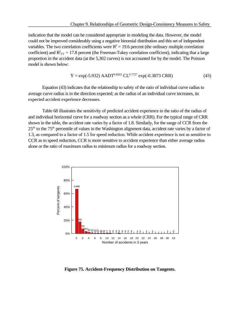
Chapter 9. Relationships of Geometric Design-Consistency Measures to Safety
0%
20%
40%
60%
80%
100%
3,499
916
37216791 52 2321 16 14 7 6 3 3 9 4 4 2 4 1 1 1 1 1 2
Number of accidents in 3 years
Per
cent
of t
ange
nts
0 2 4 6 8 10 12 14 16 18 20 22 24 26 28 30 32
indication that the model can be considered appropriate in modeling the data. However, the modelcould not be improved considerably using a negative binomial distribution and this set of independentvariables. The two correlation coefficients were R2 = 19.6 percent (the ordinary multiple correlationcoefficient) and R2
FT = 17.8 percent (the Freeman-Tukey correlation coefficient), indicating that a largeproportion in the accident data (at the 5,302 curves) is not accounted for by the model. The Poissonmodel is shown below:
Y = exp(-5.932) AADT0.8265 CL0.7727 exp(-0.3873 CRR) (43)
Equation (43) indicates that the relationship to safety of the ratio of individual curve radius toaverage curve radius is in the direction expected; as the radius of an individual curve increases, itsexpected accident experience decreases.
Table 68 illustrates the sensitivity of predicted accident experience to the ratio of the radius ofand individual horizontal curve for a roadway section as a whole (CRR). For the typical range of CRRshown in the table, the accident rate varies by a factor of 1.8. Similarly, for the range of CCR from the25th to the 75th percentile of values in the Washington alignment data, accident rate varies by a factor of1.3, as compared to a factor of 1.5 for speed reduction. While accident experience is not as sensitive toCCR as to speed reduction, CCR is more sensitive to accident experience than either average radiusalone or the ratio of maximum radius to minimum radius for a roadway section.
Figure 75. Accident-Frequency Distribution on Tangents.
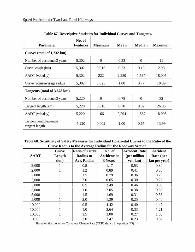
Speed Prediction for Two-Lane Rural Highways
Table 67. Descriptive Statistics for Individual Curves and Tangents.
ParameterNo. of
Features Minimum Mean Median Maximum
Curves (total of 1,232 km)
Number of accidents/3 years 5,302 0 0.33 0 11
Curve length (km) 5,302 0.016 0.23 0.18 2.98
AADT (veh/day) 5,302 222 2,280 1,567 18,005
Curve radius/average radius 5,302 0.025 1.00 0.77 10.89
Tangents (total of 3,678 km)
Number of accidents/3 years 5,220 0 0.78 0 32
Tangent length (km) 5,220 0.016 0.70 0.32 26.06
AADT (veh/day) 5,220 166 2,294 1,567 18,005
Tangent length/average tangent length
5,220 0.002 1.00 0.65 13.99
Table 68. Sensitivity of Safety Measures for Individual Horizontal Curves to the Ratio of theCurve Radius to the Average Radius for the Roadway Section.
AADTCurveLength(km)
Ratio of CurveRadius to
Ave. Radius
No. ofAccidents in
3 Years a
Accident Rate(per million
veh-km)
AccidentRate (per
km per year) 2,000 1 0.5 1.17 0.53 0.39 2,000 1 1.2 0.89 0.41 0.30 2,000 1 1.5 0.79 0.36 0.26 2,000 1 2.0 0.65 0.30 0.22 5,000 1 0.5 2.49 0.46 0.83 5,000 1 1.0 2.05 0.38 0.68 5,000 1 1.5 1.69 0.31 0.56 5,000 1 2.0 1.39 0.25 0.4610,000 1 0.5 4.42 0.40 1.4710,000 1 1.0 3.64 0.33 1.2110,000 1 1.5 3.00 0.27 1.0010,000 1 2.0 2.47 0.23 0.82
a Based on the model for Curvature Change Rate (CCR) shown in equation (43).

Chapter 9. Relationships of Geometric Design-Consistency Measures to Safety
Tangents
Both parameters included in the model for tangents—AADT and ratio of tangent length(RTL)—were statistically significant at the 95-percent confidence level. Indeed, the significance levelfor both parameters was less than 0.0001. In order of importance of their contribution in explaining thevariability in the data (as measured by their chi-square values), the parameters ranked as follows:log(AADT) (?2 = 2,997) and RTL (?2 = 1,567). The deviance for this Poisson model was 1.538 and itsPearson ?2 was 2.413. These goodness-of-fit measures are not satisfactory; other modeling approachesmight improve this model. The two correlation coefficients were R2 = 11.0 percent (the ordinarymultiple correlation coefficient) and R2
FT = 26.6 percent (the Freeman-Tukey correlation coefficient),indicating that only a limited proportion of the variance in the accident data (at the 5,220 tangents) isaccounted for by the two independent variables. The Poisson model is shown below:
Y = exp(-9.0706) AADT1.0786 exp(0.3438 RTL) (44)
While the model in equation (44) would not be very satisfactory as a predictive tool, it does indicatethat the ratio of individual tangent length to average tangent length has a statistically significantrelationship to accident frequency. This relationship indicates that accident frequency increases as anindividual tangent becomes longer relative to the average tangent length. Although RTL is statisticallysignificant in the model in equation (44), RTL is not recommended as a design-consistency measurebecause of the uncertainty in the interpretation of the appropriate direction of its relationship to accidentfrequency.
CONCLUSIONS
The statistical models developed in this chapter are not intended for use as accident predictivemodels, but rather are intended to illustrate the nature of the relationship of candidate design-consistency measures to safety. Of the candidate design-consistency measures, four have relationshipsto accident frequency that are statistically significant and appear to be sensitive enough that they may bepotentially useful in a design-consistency methodology. These four candidate design-consistencymeasures are:
• Predicted speed reduction by motorists on a horizontal curve relative to the precedingcurve or tangent.
• Ratio of an individual curve radius to the average radius for the roadway section as awhole.
• Average rate of vertical curvature on a roadway section.• Average radius of curvature on a roadway section.
Thus, these measures appear promising for assessing the design consistency of roadway alignments.

Speed Prediction for Two-Lane Rural Highways
Of these candidate design-consistency measures, the speed reduction on a horizontal curverelative to the preceding curve or tangent clearly has the strongest and most sensitive relationship toaccident frequency. The evaluation has shown that the speed reduction on a horizontal curve is a betterpredictor of accident frequency than the radius of that curve. This makes a strong case that a design-consistency methodology based on speed reduction provides a better method for anticipating andimproving the potential safety performance of a proposed alignment alternative than a review ofhorizontal curve radii alone.
Accident frequency is not as sensitive to the alignment indices reviewed as it is to the speedreduction for individual horizontal curves. The alignment index that has the greatest sensitivity toaccident frequency is the ratio of an individual curve radius to the average radius for the roadwaysection as a whole. While this alignment index is potentially useful as a design-consistency measure,accident frequency is not as sensitive to it as to the speed reduction for an individual curve. In otherwords, it appears to be more useful to compare the speed on horizontal curves to the speed on itsimmediately adjacent geometric features than to compare its radius to the average radius for theroadway section as a whole.
The average rate of vertical curvature for a roadway section and the average radius ofhorizontal curves for a roadway section also show promise as design-consistency measures. However,neither of these measures appears to be as appropriate a measure of design consistency as the speedreduction for individual horizontal curves.
The remaining alignment indices evaluated do not appear to be appropriate design-consistencymeasures because of their weak or ambiguous relationships to accident frequency. Thus, the followingalignment indices are not recommended as design-consistency measures:
• Ratio of maximum radius of curvature to minimum radius of curvature for all horizontalcurves on a roadway section.
• Average tangent length for a roadway section.
• Ratio of an individual tangent length to the average tangent length for the roadwaysection as a whole.

10. SUMMARY, FINDINGS, CONCLUSIONS,AND RECOMMENDATIONS
SUMMARY
Design consistency refers to the conformance of a highway’s geometry with driver expectancy.Drivers make fewer errors in the vicinity of geometric features that conform with their expectations. Atechnique to evaluate the consistency of a design is to evaluate changes in operating speeds along analignment. If the speed is relatively constant for an alignment with one or more exceptions, such as at ahorizontal curve, then that feature should be evaluated and perhaps redesigned. To use operating speedas a consistency tool requires the ability to accurately predict speeds as a function of the roadwaygeometry. In this research project, several different efforts were undertaken to predict operating speedsfor different conditions, such as on horizontal and vertical curves, on tangent sections, and prior to orafter a horizontal curve. Speed data were collected at more than 211 two-lane rural highway sites foruse in the project (176 simple circular curves, vertical curves, and their approach tangents; 12 spiraledcircular curves and their approach tangents; and 21 simple circular curve sites where detailedacceleration/deceleration measurements were obtained).
The data were used to develop speed-prediction equations for horizontal and verticalalignments, to analyze the effects of spiral curves, and to evaluate whether speed is different at the studysites for different vehicle types. Regression equations were developed for passenger cars for mostcombinations of horizontal and vertical alignment. For some of the combinations, however, sample sizeswere not large enough for the equations to be considered definitive. The analysis of spiral curves foundthat the use of a spiral did not result in a significant difference in speed when compared to similar sitesthat did not have spirals. Because most of the study sites had few spot-speed observations for trucksand recreational vehicles, a limited analysis was performed for those sites with a minimum of 10observations. The limited graphical analysis on trucks and recreational vehicles found similar speedtrends between the different vehicle types. Therefore, a design-consistency evaluation should use theequations based on passenger car data.
The collected data were also used to determine whether alignment indices can accuratelypredict speeds on a tangent. In addition, other possible influences of motorists’ desired speeds wereexamined. The findings of this research indicated that combinations of alignment indices and othergeometric variables were not able to significantly predict the 85th percentile speeds of motorists on longtangents of two-lane rural highways. For those situations when a vehicle is traveling on an upgrade ordowngrade, the equations used in the TWOPAS model can be used to estimate speeds for differentvehicle types. The models can be used to predict the speed of the vehicle at any point on the grade if itsinitial speed at the entry to the grade is known.
Data were collected and analyzed at 21 sites to determine appropriate acceleration anddeceleration values prior to and after a horizontal curve. The acceleration and deceleration assumptions

Speed Prediction for Two-Lane Rural Highways
and rates involved in the formulation of the original model presented in FHWA-RD-94-034 wereexamined. New acceleration/deceleration models were constructed from the data to consider theeffects of the curve radius.
The speed-prediction models developed in a previous FHWA project and in this project werevalidated. The objectives of the validation efforts were to evaluate the assumptions and validate theaccuracy with which the previous and newly developed speed-profile equations accurately predictspeeds as a function of highway geometry; and as necessary, refine, reformulate, and recalibrate themodels. The subtasks involved in the validation efforts include performing internal and externalvalidations to compare equation-estimated and observed values.
Based on the results from the validation efforts and the desire to use as many sites as wereavailable, new speed-prediction equations were developed using all data collected in this study. Theseequations, along with the findings from other tasks, were incorporated into a speed- profile model. Themodel can be used to evaluate the design consistency of the roadway or can be used to develop aspeed profile for an alignment. The model considers both horizontal and vertical curvature and theacceleration or deceleration behavior as a vehicle moves from one feature to another.
Both predicted speed on a facility and alignment indices have been suggested as geometricdesign-consistency measures. This study included a demonstration of the relationship between thesemeasures and safety. Of the candidate design-consistency measures, the predicted-speed reduction ona horizontal curve relative to the preceding curve or tangent clearly has the strongest and most sensitiverelationship to accident frequency.
FINDINGS
The findings from the speed-prediction efforts are subdivided into speeds on curves, alignmentindices, TWOPAS, acceleration and deceleration rates, validation of speed-prediction equations,speed-profile model, and relationship of design-consistency measures to safety. The following are thelist of findings within each of these categories.
Speeds on Curves
Horizontal Curves on Grades
• For passenger vehicles, radius was the only significant independent variable inpredicting 85th percentile speeds for all alignment combinations that included ahorizontal curve on grade. The best form of the independent variable in regressionequations is 1/R.

Chapter 10. Summary, Findings, Conclusions, and Recommendations
• Operating speeds on horizontal curves are very similar to speeds on long tangents whenthe radius is greater than or equal to approximately 800 m. Under this condition, thegrade of the section may control the selection of speeds, and the contribution of thehorizontal radius is negligible.
• Operating speeds on horizontal curves drop sharply when the radius is less than 250 m.
Vertical Curves on Horizontal Tangents
• Passenger vehicle speeds on limited sight-distance vertical curves on horizontal tangentscould be predicted using the rate of vertical curvature as the independent variable. Thebest form of the independent variable in regression equations is 1/K.
• A statistically significant regression equation could not be found for crest curves wherethe sight distance is not limited; therefore, the desired speed for long tangents isassumed.
• For sag curves on horizontal tangents, the plot of the seven available data points and theregression analysis indicate that the desired speed on long tangents should be assumed.
Horizontal Curves Combined With Vertical Curves
• For non-limited sight-distance crest vertical curves in combination with horizontalcurves, the lowest speed of the speeds predicted using the equations developed forhorizontal curves on grades or the assumed desired speed should be used. Thecollected speed data for that condition were generally for large horizontal curve radiiwith several of the speeds being above 100 km/h. Drivers may not have felt the need toreduce their speed in response to the geometry for these large radius horizontal curves.
• For the horizontal curvature combined with either sag or limited sight-distance crestvertical curves, the radius of the horizontal curve was the best predictor of speed.
Spirals
• There is no difference in 85th percentile speeds at the midpoint on circular curves fromthose with spiral transitions.
Other Vehicle Types
• The data for all truck types and recreational vehicles on horizontal curves display ageneral speed behavior that is similar to that of passenger vehicles.
• The influence of grade on trucks and recreational vehicles is similar to, but larger than,the effects observed for passenger vehicles.
Alignment Indices

Speed Prediction for Two-Lane Rural Highways
• None of the alignment indices studied were statistically significant predictors of thedesired speeds of motorists on long tangents of two-lane rural highways.
• There were significant regional differences in the desired speeds of motorists on longtangents of two-lane rural highways.
• Of the geometric variables examined, only the vertical grade at the tangent sitesignificantly affected the desired speeds of motorists on long tangents of two-lane ruralhighways.
TWOPAS Vehicle-Performance Equations
C The TWOPAS vehicle-performance equations can be used to determine the speed forspecific vehicle types at any point on a grade.
Acceleration and Deceleration Rates for a Horizontal Curve
C The validation results indicate that the acceleration and deceleration assumptions employedin the previous speed-profile model are not valid for the set of study sites selected in thisstudy. The speed values predicted and the speed values measured in the field arestatistically different at the 95-percent confidence level.
C The only sites with acceleration and deceleration rates that approached 0.85 m/s2 werethose with curve radii less than 250 m.
C New models were developed to consider the effect of curve radii on theacceleration/deceleration rates. The models were based on maximum acceleration anddeceleration rates observed at the study sites.
Validation of the Speed-Prediction Equations
• The validation of the six speed-prediction equations for horizontal and vertical curves (seetable 14) was performed by comparing the equation predicted V85 to the field observed V85
at the midpoint of the curve. The overall mean absolute percent error for the six equationswas 5.7 percent.
• Validation was also conducted for the predicted speed change between the midpoint of theapproach tangent and the midpoint of the horizontal curve. In general, the models werefound to differ from the observed change in speed between the tangent and the horizontalcurve by an average of 98 percent.
Speed-Profile Model
C A speed-profile model was developed that can be used to evaluate the design consistencyof a facility or to generate a speed profile along an alignment. The design-consistencyevaluation consists of identifying undesirable speed changes between features. The speed-prediction equations are used to predict the speeds for the features, and then the differences

Chapter 10. Summary, Findings, Conclusions, and Recommendations
in speed between successive features would be calculated. To generate a speed profile, thelowest anticipated speed would be obtained by selecting the lowest speed predicted by theselected desired speed on tangent, the speed-prediction equations, and/or the TWOPASmodel. This speed would then be adjusted prior to and departing from curves using theacceleration and deceleration values determined in this project.
• The speed-profile model developed in the research appears to provide a suitable basis forthe IHSDM design-consistency module.
Relationship of Design-Consistency Measures to Safety
C Of the candidate design-consistency measures, four have relationships to accidentfrequency that are statistically significant and appear to be sensitive enough that they may bepotentially useful in a design-consistency methodology. These four candidate design-consistency measures are:S Predicted speed reduction by motorists on a horizontal curve relative to the
preceding curve or tangent.S Ratio of an individual curve radius to the average radius for the roadway
section as a whole.S Average rate of vertical curvature on a roadway section.S Average radius of curvature on a roadway section.
C Of these candidate design-consistency measures, the speed reduction on a horizontal curverelative to the preceding curve or tangent clearly has the strongest and most sensitiverelationship to accident frequency.
CONCLUSIONS
The following general conclusions were developed based on the findings of the study:
• This research produced speed-prediction equations that can be used to calculate theexpected speed along an alignment that includes both horizontal and vertical curvature.
• The alignment indices did not explain the variation in measured speeds on long tangents.

Speed Prediction for Two-Lane Rural Highways
• The average 85th percentile speed per State for long tangents ranged from 93 to 104 km/h.Based on the data and engineering judgment, the operating speeds on tangents and themaximum operating speeds on horizontal curves could be rounded to 100 km/h.
• After establishing that current acceleration and deceleration rates and assumptions are notvalid, at least for the sites selected in this study, new models were developed that predictacceleration and deceleration rates in the vicinity of a horizontal curve as a function of curveradius. Models were not developed for vertical curves or for horizontal/vertical combinedcurves.
• The six speed-prediction equations presented in chapter 3 performed well in the validationeffort with a range of mean absolute percent error between 4.1 percent and 10 percent.The predicted speed difference between the midpoint of the tangent and the horizontalcurve (calculated using the deceleration findings from chapter 6 and the speed-predictionequations presented in chapter 3) did not compare well with the observed speed reduction.The range of mean absolute percent error was 87 percent to 107 percent for the fourconditions studied.
• The various findings from this study were used to develop a speed-profile model. Thismodel can be used to evaluate the design consistency of a facility or to generate a speedprofile along an alignment.
• Of the different alternatives examined, a design-consistency methodology based onpredicted speed reductions was the best identified.
• The IHSDM should contain a design-consistency module based on the speed-profile modeldeveloped in this research.
RECOMMENDATIONS
The following recommendations (listed in order of relative priority) are made based on thefindings and conclusions of this study:
• Additional insight into the influences of speeds on tangent sections of various lengths andgrades is needed. This would greatly enhance the effectiveness of any speed-profile modelbecause it would validate the assumptions currently being made.
• The acceleration and deceleration models developed here were exclusively related to theimpact of the horizontal curve. It is recommended that a similar effort be undertaken toassess the impact of vertical curves, as well as horizontal-vertical combinations onacceleration and deceleration profiles.

Chapter 10. Summary, Findings, Conclusions, and Recommendations
• Further research should be conducted to extend all aspects of this research, such as speed-prediction equations, acceleration/deceleration behavior, and the design-consistencymodule speed-profile model, to roadway types other than two-lane rural highways.
• Further refinements should be made to the IHSDM design-consistency module in futureresearch to include a capability of identifying design inconsistencies based on factors otherthan horizontal and vertical alignment. Such factors might include intersections, driveways,and auxiliary lanes.
• Further research should be conducted on estimating operating speeds of trucks andrecreational vehicles for different horizontal and vertical curves. Additional data arerequired to develop regression models to estimate operating speeds of trucks and RVs.
• Further research is needed on the ability of alignment indices to estimate desired speeds ofmotorists on long tangents of two-lane rural highways. Gaps in the existing databaseincluded roads with posted speeds greater than 88.5 km/h (55 mph) and alignment indicesnear the maximum values of those in this study.
• Because the safety evaluation demonstrated that predicted-speed reduction has thestrongest relationship to accident frequency, speed reduction should be the primarymeasure in design-consistency methodology for horizontal and vertical curvature. Toaccomplish this, better methods to predict speeds need to be investigated. Alignmentindices may be appropriate measures to supplement speed reduction in a design-consistency methodology, but they should not be considered as the primary measure.