Version 1

Special Relativity

Milind V. Purohit (U. of South Carolina)

Abstract

Contents

1 Introduction 2

2 Maxwell’s Equations and Electromagnetic Waves 2

3 Galilean Transformations 3

4 4-vectors and Lorentz Transformations 3

5 Invariants and Time Dilation 5

6 Tensors and the metric 7

7 Contravariant and Covariant Four-Vectors 7

8 Velocity Addition 8

9 The Lorentz Trnasformation Matrix 10

10 Time Dilation and Length Contraction 1110.1 Time Dilation . . . . . . . . . . . . . . . . . . . . . . . . . . . . . . . . . . . 1110.2 Length contraction . . . . . . . . . . . . . . . . . . . . . . . . . . . . . . . . 11

11 *Decay kinematics 1211.1 Two-body decays . . . . . . . . . . . . . . . . . . . . . . . . . . . . . . . . . 1211.2 Two-body phase space . . . . . . . . . . . . . . . . . . . . . . . . . . . . . . 12

12 *Phase Space 1212.1 Lorentz Invariant Phase Space (LIPS) . . . . . . . . . . . . . . . . . . . . . . 1212.2 Transformation of particle distribution functions . . . . . . . . . . . . . . . . 15

13 Rapidity 15

14 *The Electromagnetic Field Tensor 17

15 Covariant form for the Lorentz Force 1715.1 4-Forces . . . . . . . . . . . . . . . . . . . . . . . . . . . . . . . . . . . . . . 17

16 The Action Principle 18

17 *The Spin Vector 1917.1 Introduction . . . . . . . . . . . . . . . . . . . . . . . . . . . . . . . . . . . . 1917.2 The BMT equation . . . . . . . . . . . . . . . . . . . . . . . . . . . . . . . . 20

18 References 21

1

1 Introduction

Special Relativity occupies such a special place in the education and imagination of physicsstudents, that it hardly needs an introduction. We will therefore abbreviate the prefatorymaterial and proceed rapidly to applications of special relativity in particle physics.

Particle physicists deal daily with speeds close to the speed of light. In this high-speedworld, relativity is the rule - not the exception - and we must learn to think in new ways. It isparticularly important for us to know how to transform physical quantities between framesof reference, quantities such as spacetime coordinates, energy-momentum, charge density,current, spin etc.

To do so, we must learn to treat all frames of reference as equivalent, which forces usto create laws that have the same form in all frames of reference (covariance). A practicalaspect of dealing with relativistic speeds is to capitalize on usage of invariant quantities,those which have the same value in all frames of reference.

2 Maxwell’s Equations and Electromagnetic Waves

By the year 1865 Maxwell had codified the laws of electrodynamics into his famous equations(we use units in which c = 1):

~∇× ~E = −∂t~B (1)

~∇× ~B = ∂t~E +~j (2)

~∇ · ~E = ρ (3)

~∇ · ~B = 0 (4)

You know already that equations (1) and (4) are automatically satisfied when the electricand magnetic fields are written in terms of a scalar potential field φ and a vector potentialfield ~A as follows:

~E = −∇φ− ∂t~A (5)

~B = ~∇× ~A (6)

We can form a wave equation for electromagnetic waves in empty space by taking, forinstance, the curl of Eq. 2 and using the vector identity

~∇× ~∇× ~B = ∇(~∇ · ~B)−∇2 ~B (7)

to get, using Eq. (4),

∇2 ~B − 1

c2∂2

t~B = 0 (8)

where we have deliberately displayed c2 to indicate the speed of the wave. Similarly, one cantake the curl of Eq. (1) to find a similar equation for E:

∇2 ~E − 1

c2∂2

t~E = 0 (9)

2

We see thus that the components of ~E and ~B satisfy wave equations. You are familiarat least with the plane wave solutions

~E ∼ ~E0ei(~k·~x−ωt) (10)

~B ∼ ~B0ei(~k·~x−ωt) (11)

When these solutions are plugged into the wave equations (9) and (8) we find the familiarcondition ω = kc for an electromagnetic wave.

3 Galilean Transformations

Soon after the discovery of these equations, it became clear that the wave equations werenot invariant under Galilean transformations. These transformations refer to the usual, non-relativistic, transformations of coordinates between reference frames moving with a uniformvelocity with respect to each other. For instance, if reference frame S ′ is moving at speedv in the x-direction relative to frame S, then the space and time coordinates x′, y′, z′, t′

in this primed frame (S ′) are related to the coordinates in the unprimed frame (S) by theGalilean transformation equations

x′ = x− vt (12)

y′ = y (13)

z′ = z (14)

t′ = t (15)

Notice that the coordinates transverse to the motion, i.e., x and y, do not change, and moreimportantly, notice the concept of absolute time: in the Galilean view time is the same in allframes of reference. (Of course, this is what our intuition tells us, but we know now that ourintuition is wrong!) It is possible to show, see problem ??, that this set of equations does notleave the electromagnetic wave equations invariant. Non-invariance of the wave equation indifferent frames of reference implies that there must be a special frame of reference in whichc is the speed of light.

Indeed, a lot of effort was spent in trying to find this special frame (the frame of thesupposed ether, which was also the medium supposed to carry the electromagnetic waves).One such experiment, carried out in 1887, was the exquisitely sensitive and therefore justlyfamous Michelson-Morley experiment. Interpreting the null result of this experiment (thespeed of light appeared to be the same in all frames of reference) led to numerous ideas.

4 4-vectors and Lorentz Transformations

Many famous physicists tried their hand at interpreting the null result of the Michelson-Morley experiment, including Lorentz, Fitzgerald, Poincare and Larmor. Unfortunately,none of the explanations was satisfactory, although the process did produce the expressionsused today in the Lorentz transformations. It was Einstein who provided the proper in-terpretation, and it is his theory of special relativity that we turn to next. [Note though

3

that Einstein, while aware of the Michelson-Morley experiment, claimed not to be greatlyinfluenced by it.]

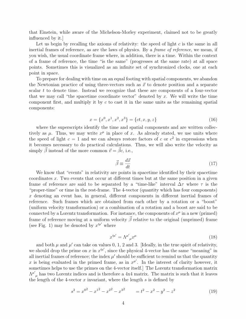
Let us begin by recalling the axioms of relativity: the speed of light c is the same in allinertial frames of reference, as are the laws of physics. By a frame of reference, we mean, ifyou wish, the usual coordinate frame where, in addition, there is a time. Within the contextof a frame of reference, the time “is the same” (progresses at the same rate) at all spacepoints. Sometimes this is visualized as an infinite set of synchronized clocks, one at eachpoint in space.

To prepare for dealing with time on an equal footing with spatial components, we abandonthe Newtonian practice of using three-vectors such as ~x to denote position and a separatescalar t to denote time. Instead we recognize that these are components of a four-vectorthat we may call “the spacetime coordinate vector” denoted by x. We will write the timecomponent first, and multiply it by c to cast it in the same units as the remaining spatialcomponents:

x = x0, x1, x2, x3 = ct, x, y, z (16)

where the superscripts identify the time and spatial components and are written collec-tively as µ. Thus, we may write xµ in place of x. As already stated, we use units wherethe speed of light c = 1 and we can always restore factors of c or c2 in expressions whenit becomes necessary to do practical calculations. Thus, we will also write the velocity assimply ~β instead of the more common ~v = ~βc, i.e.,

~β ≡ d~x

dt(17)

We know that “events” in relativity are points in spacetime identified by their spacetimecoordinates x. Two events that occur at different times but at the same position in a givenframe of reference are said to be separated by a “time-like” interval ∆τ where τ is the“proper-time” or time in the rest-frame. The 4-vector (quantity which has four components)x denoting an event has, in general, different components in different inertial frames ofreference. Such frames which are obtained from each other by a rotation or a “boost”(uniform velocity transformation) or a combination of a rotation and a boost are said to beconnected by a Lorentz transformation. For instance, the components of xµ in a new (primed)

frame of reference moving at a uniform velocity ~β relative to the original (unprimed) frame(see Fig. 1) may be denoted by x′µ′

where

x′µ′= Λµ′

µxµ (18)

and both µ and µ′ can take on values 0, 1, 2 and 3. [Ideally, in the true spirit of relativity,we should drop the prime on x in x′µ′

, since the physical 4-vector has the same “meaning” inall inertial frames of reference; the index µ′ should be sufficient to remind us that the quantityx is being evaluated in the primed frame, as in xµ′

. In the interest of clarity however, itsometimes helps to use the primes on the 4-vector itself.] The Lorentz transformation matrixΛµ′

µ has two Lorentz indices and is therefore a 4x4 matrix. The matrix is such that it leavesthe length of the 4-vector x invariant, where the length s is defined by

s2 = x02 − x12 − x22 − x32= t2 − x2 − y2 − z2 (19)

4

in our units where c = 1. This is similar to ordinary rotations in 3-dimensional spacewhere the components of the 3-vector ~x are transformed by a rotation matrix R in a waythat leaves the length of the vector invariant, except that we define the “length” a littledifferently in 4-dimensional spacetime (notice the minus signs in equation 19).

We may justify Eq. 19 by assuming that the speed of light is the same in all frames ofreference. Consider two frames of reference, a primed frame and an unprimed frame, movingrelative to each other along, say, the x-axis. Consider how we may describe the propagationof a flash of light in the two frames. If we choose the location of the flash to be the originof both frames and ask how the light wavefront propagates in the +x-direction, we see thatboth x and x′ are given by similar equations:

x = ct (20)

and

x′ = ct′ (21)

Generalizing to arbitrary direction leads us to require that the radius of the light wave-front obeys an equation similar to Eq. 19:

x2 + y2 + z2 = c2t2 (22)

and in the primed frame,

x′2 + y′2+ z′

2= c2t′

2. (23)

[We now revert to our convention c = 1.]

5 Invariants and Time Dilation

Let us use the invariance of “length” to deduce an important quantity called γ. In therest frame of a particle an infinitesimal time interval between two events (the particle’s 4-positions) is denoted by dτ . We may relate this to intervals in another frame of referenceusing the invariant length s as follows:

ds2 = dτ 2 = dt2 − dx2 − dy2 − dz2 = dt2(1− β2) (24)

We see thus that the time interval in another frame of reference is always longer thandτ , an effect known as “time dilation”. We conclude that the ratio of these time intervals γis given by

γ ≡ dt

dτ=

1√1− β2

(25)

5

S⁄S

L t

β

Figure 1: We typcally transform physical quantities between frames of reference, labeledS and S ′ in this case. The length L and time t in the unprimed frame of reference willtransform to L′ and t′ in the primed frame.

6

6 Tensors and the metric

In general, we try to use “invariant” quantities like ds, i.e., quantities that are the samein all frames of reference, as often as possible in our thinking and calculations. Further,we define contravariant 4-vectors as those 4-vectors which transform in the same way as xµ

under Lorentz transformations, i.e., as in equation 18. Indeed, objects with more than oneindex which transform like xµ (one transformation matrix per index) are called tensors ofrank-2, rank-3 and so on. For example, the rank-2 tensor T µν will transform as follows:

T ′µ′ν′= Λµ′

µΛν′

νTµν (26)

The invariants we use such as s2 = x2 may be defined using a “metric tensor” called gµν .For the flat Minkowski spacetime of special relativity gµν is also referred to as ηµν and isgiven by

gµν = ηµν =

1 0 0 00 −1 0 00 0 −1 00 0 0 −1

(27)

We define the inverse matrix (gµν)−1 as gµν , which is the same as gµν in our case of specialrelativity.

gµν =

1 0 0 00 −1 0 00 0 −1 00 0 0 −1

(28)

Now, we may define the length “s” of a vector by

s2 = gµνxµxν = x02 − x12 − x22 − x32

(29)

where we adopt the “Einstein summation convention” which says to sum over all repeatedindices.

7 Contravariant and Covariant Four-Vectors

Equation 29 above can also be viewed as expressing the “inner” or “dot” product of xµ andxµ, where the “covariant” vector xµ is formed by “lowering” the index µ:

xµ = gµνxν = t,−x,−y,−z (30)

In general, we use the metric gµν or gµν to “raise” or “lower” indices. Thus our dotproduct above may be written

s2 = x · x = xµxµ = xµxµ = gµνx

µxν = x02 − x12 − x22 − x32(31)

In our case, where gµν is simply ηµν , the only effect of lowering the index is to change thesign of the spatial components. However, you can see how a more complicated gµν would

7

lead to a different result. In general, when a lower and upper index are the same in anexpression, the resulting summation is called a “contraction”.

More important than the sign change due to lowering is the transformation property ofxµ, which is somewhat different from that of xµ.

Let us consider once again the Lorentz transformation given by equation 18 which ex-presses the transformed 4-vector in terms of the original. Of course, we could invert thatrelation to obtain

xµ = Λ µµ′ x′µ′

(32)

where Λ µµ′ is different from and written differently from its inverse Λµ′

µ (the first indexis lower, not the second; see also section 9 below).

s2 = xµxµ = x02 − x12 − x22 − x32(33)

where

xµ = gµνxν (34)

How does the “covariant” vector xµ transform under Lorentz transformations? Using theraising and lowering properties of the metric defined above we see that

x′µ′ = gµ′ν′x′ν′

= gµ′ν′Λν′

νxν = gµ′ν′Λν′

νgµνxµ = Λ µ

µ′ xµ (35)

i.e., xµ transforms according to the inverse Lorentz transformation (for explicit examplesof Λ and its inverse, see Eqn. 49 and Eqn. 50 below). Similarly, we can investigate thetransformation of the derivative with respect to xµ:

∂µ ≡∂

∂xµ(36)

Using equation 32 and the chain rule of differentiation we see that

∂µ′ ≡ ∂

∂x′µ′ =∂

∂xµ

∂xµ

∂x′µ′ = Λ µµ′ ∂µ (37)

This is the same transformation law as for xµ in equation 35 above. Indeed, any vectorthat transforms in the same way as ∂µ, i.e., according to equation 37 is said to be a “covariant”vector.

8 Velocity Addition

As an example of using invariant quantities, let us re-visit the formula for velocity addition,familiar from a first course on special relativity. According to pre-relativistic (Galilean)physics, if particle A is moving along the x-direction with velocity vA and particle B isapproaching A in the opposite direction with velocity −vB, then their relative velocity, i.e.,velocity of B in A’s rest-frame is simply vA + vB. We know that this is not the case inrelativistic physics; let us derive the correct formula. Figure 2 illustrates the problem.

First, we introduce the 4-velocity vµ defined by

8

x

y

A B

Figure 2: In pre-relativistic physics, the velocity of B in A’s rest-frame is simply vA + vB.The correct formula however is equation 44.

vµ ≡ dxµ

dτ= γ, γ~β (38)

where we have used equations 17 and 25. Notice that

vµvµ = 1 (39)

With this definition of 4-velocity, we may write the velocities of A and B as

vµA = γA, γA

~βA (40)

vµB = γB,−γB

~βB (41)

Denoting quantities in A’s rest-frame by primes, we also have

v′µA = 1,~0 (42)

v′µB = γ′B,−γ′

B~β′

B

Now we are in a position to utilize the invariant quantity vA · vB that we may form fromthe velocities of A and B. Since it is an invariant, we may evaluate it in the primed andunprimed frames of reference and equate the two results:

9

vA · vB = v′A · v′BγAγB + γAγBβAβB = γ′

B (43)

Writing each γ in terms of the corresponding β (using equation 25) and solving for β′B

we find that the solution which reduces to the correct non-relativistic expression is

β′B =

βA + βB

1 + βAβB

(44)

9 The Lorentz Trnasformation Matrix

Let us work out explicitly the matrix for a boost. Consider, in particular, the boost shown infigure 1. The origin of the S ′ frame has a velocity ~β in the unprimed S frame, for simplicitywe may assume that ~β is entirely along the negative x-direction: ~β = −βx. We seek todetermine the matrix Λµ′

µ which connects xµ′to xµ via Eqn. 18 or its inverse, Eqn. 32.

Using these equations we see that

xµ′= Λµ′

µxµ = Λµ′

µΛ µµ′ x′µ′

(45)

Since the y and z directions are unaffected, we can look initially for a 2x2 matrix thatrelates x′ and t′ to x and t. This can then become a submatrix of Λµ′

µ. A simple rotationmatrix such as

R =(

cos θ − sin θsin θ cos θ

)(46)

will clearly not do the trick. Why not? Rotation matrices will not work because thesines and cosines they are based on will preserve lengths, such as t2 + x2, using the propertysin2 θ + cos2 θ = 1. Here however, we need to conserve the difference t2 − x2 (see Eq. 19).We can achieve this by the transformation matrix equation(

t′

x′

)=(

γ γβγβ γ

)(tx

)(47)

which can be inverted immediately to give(tx

)=(

γ −γβ−γβ γ

)(t′

x′

). (48)

Finally then, we can write our boost matrices for the boost described by Fig. 1:

Λµ′

µ =

γ 0 0 γβ0 1 0 00 0 1 0

γβ 0 0 γ

(49)

and

10

Λ µµ′ =

γ 0 0 −γβ0 1 0 00 0 1 0

−γβ 0 0 γ

. (50)

It is easy to verify that the determinants of these two transformation matrices are both+1 and that the matrices are the inverse of each other, i.e., that

Λµ′

µΛ µν′ = δµ′

ν′ .

Notice also that the matrices transform into each other when we replace β by −β, as weshould expect.

The Lorentz transformation given by equations (45) and (49) is often written in a moregeneral way to emphasize the directions parallel and perpendicular to the boost:

t′ = γ(t + βx‖) (51)

x′‖ = γ(x‖ + βt) (52)

~x′⊥ = ~x⊥ (53)

10 Time Dilation and Length Contraction

10.1 Time Dilation

Consider a particle at a fixed point ~x in a frame of reference in which it is at rest (knownhereafter as its “rest frame”). If a “proper time” τ elapses in a particle’s rest frame, thenaccording to equation (51) the time elapsed in any other frame of reference will be γτ , i.e.,longer by the relativistic boost factor γ. This effect is known as “time dilation” and isso commonly observed in experiments as to be second nature to every practicing particlephysicist. Without this effect, muons produced in the upper atmosphere by incoming cosmicrays would not live long enough to rain down on us at earth level, and the observation oflarge numbers of short-lived particles would become rather difficult indeed.

10.2 Length contraction

Contrary to the apparent “dilation” (or lengthening) of time, lengths appear to be shorteror “contracted” when viewed from frames of reference in which the object whose length ismeasured is moving. We have to be a bit more careful in deriving this effect though. Letus assume that the primed frame S ′ is moving at speed v in the x-direction relative to theunprimed frame S, in which an object is at rest. The two ends of the object are measured tobe x1 and x2 at time t in the rest frame. In general, we must not ask for the correspondingpoints x′

1 and x′2 in S ′ since these are not measurements at the same time t′. Instead, we

should consider measurements x′1 and x′

2 at the same time t′. We see that since

x1 = γ(x′1 + βt′) (54)

x2 = γ(x′2 + βt′) (55)

11

the length L′ ≡ (x′2 − x′

1) measured in the S ′ frame is shorter than the “proper length”L ≡ (x2−x1) measured in the rest frame. Note that it does not matter that the measurementsx′

1 and x′2 which are required to be simultaneous in the S ′ frame are not so in the rest frame

S; in the rest frame we expect that the measurements of the two ends of the object can takeplace at the same time or at different times with no difference in the result.

11 *Decay kinematics

11.1 Two-body decays

We emphasized that in the rest frame S of the decaying particle of mass M , both decayproducts have the same momentum. The decay products come out back-to-back in thisframe of reference, each with momentum p∗. The angles specifying the decay direction ofone of the particles, let’s call them θ∗ and φ∗ in S, are arbitrary. One should be able tocompute the corresponding angles in the lab frame if the decaying particle has a velocity ~βin the lab frame S ′.

11.2 Two-body phase space

We introduced the Mandelstam variables s, t and u for the case of two-body scattering:

1 + 2 → 3 + 4 (56)

Consider the significance of each of these. It can be shown that√

s is the energy availablein the c.m. frame, while t and u are related to the scattering angle in the c.m. frame. Wediscussed s-, t-, and u-channels.

12 *Phase Space

12.1 Lorentz Invariant Phase Space (LIPS)

The concept of phase space is one we will introduce more clearly later; here we will emphasizeaspects deriving from special relativity. Quantum Field theory tells us that Fermi’s Goldenrule, which gives transition rates in terms of the square of a matrix element times the densityof states can be extended in relativistic processes. The density of states is replaced by a termpopularly called “phase space”, or “Lorentz Invariant Phase Space” (LIPS). This consists ofa product of 1-body momentum space quantities d3p/2E times a delta function embodying 4-momentum conservation in the decay of a particle with 4-momentum P into many particles,each with 4-momentum pi:

LIPS =

[∏i

d3pi

2Ei

]δ(4)(P −

∑i

pi)

Note that there need not be a real decay; the formalism is used even in interactions whereP simply denotes the total available 4-momentum for the “decay” into n particles.

12

We can see that each (d3p/2E) term is Lorentz invariant in a variety of ways; it will beuseful for our understanding to do so. Due to the factors of γ that divide and multiply lengthand time in a Lorentz transformation, we can immediately see that d4x is Lorentz-invariant,as is any other such differential 4-dimensional volume element such as d4p. For any realparticle, the relation E2 = ~p2 +m2 is a constraint that prevents it from occupying any pointin 4-dimensional momentum space; we may impose the constraint and find that

∫d4p δ(p2 −m2) =

d3p

2E

We could also explicitly show that (d3p/2E) is Lorentz invariant as follows. Differentiat-ing the relation E2 = ~p2 + m2 we find that

EdE = pdp (where p refers to the magnitude of the 3-momentum)

If only one component of ~p is allowed to vary, for instance the component parallel to a givenaxis, then EdE = p‖dp‖. Under a Lorentz transformation (d3p/2E) → (d3p′/2E ′).Without loss of generality we can split the 3-momentum into components parallel to (‖)or perpendicular (⊥) to the boost direction. Then, we find (ignoring the perpendicularcomponents which do not change) that

dp′‖2E ′ =

d(γ(p‖ + βE))

γ(E + βp‖)= dp‖(1 + β(p‖/E)) =

dp‖E

[This follows immediately from the fact that the number of particles N(~p)d3p = (E N(~p))(d3p/E)should be Lorentz invariant; therefore E N(~p) is Lorentz invariant.]

We showed that d3p/2E is a Lorentz-invariant element of momentum space for any par-ticle. We used this to derive the two-body and three-body phase space formulas in the restframe of the decaying particle of mass M :

dΦ2 ≡∫ d3p1

2E1

d3p2

2E2

δ(4)(Pf − Pi)

(2π)6

=p1

4M

dΩ1

(2π)6(57)

The important thing here is to recognize that the two-body phase space is proportionalto p1/M , a quantity that can vary between 0 and 0.5. If the final state particles are verylight, phase space is maximized; if the final state particle masses almost add up to the parentmass there is very little phase space.

In the 3-body case, we begin with the LIPS formula below:

dΦ3 ≡∫ d3p1

2E1

d3p2

2E2

d3p3

2E3

δ(4)(Pf − Pi)

(2π)9

=dE1dE2dΩ1dφ12

8(2π)9(58)

13

We see that we can eliminate one of the three momenta, say ~p3, by integrating over thedelta function to obtain

dΦ3 ∝∫ d3p1d

3p2

E1E2E3

δ(E − E1 − E2 − E3)

This time, the integral is a little harder to do because of the energy terms in the denominator.We begin by defining angles for particle 1 relative to some coordinate frame in which theparent particle is at rest. Then, we may write d3p1 as p2

1dp1dΩ1, where Ω1 is the solid anglefor particle 1. For particle 2 however, we may choose the direction of particle 1 as the z-axisand therefore we will express d3p2 as p2

2dp2dΩ12 where the subscript 12 refers to particle 2relative to particle 1. With these definitions we arrive at

dΦ3 ∝∫ p2

1dp1dΩ1p22dp2dΩ12

E1E2E3

δ(E − E1 − E2 − E3)

Now, for fixed momentum magnitudes p1 and p2, we see that ~p1 + ~p2 = −~p3, meaningthat

|~p1|2 + |~p2|2 + 2|~p1||~p2| cos(θ12) = |~p3|2

If we fix the magnitudes of the momenta of particles 1 and 2, we find that

2p1p2d cos(θ12) = 2p3dp3

where we have again dropped the vector symbol to indicate magnitudes of 3-momenta. Thus,we may write

dΦ3 ∝∫ p1dp1dΩ1p2dp2dφ12p3dp3

E1E2E3

δ(E − E1 − E2 − E3)

Using relation ?? we find that

dΦ3 ∝∫

dE1dE2dE3dΩ1dφ12δ(E − E1 − E2 − E3)

Now the integral over energy is trivial leading to

dΦ3 ∝∫

dE1dE2dΩ1dφ12

Often the direction variables are ignored or integrated over. For instance, if the parentparticle is spinless or unpolarized, then the angles are not informative variables and we seethat

dΦ3 ∝∫

dE1dE2 Unpolarized initial state

Finally, we can (as is usually done) cast this equation in terms of invariant mass-squaredsalone. Using, for instance,

m223 ≡ (p2 + p3)

2 = (P − p1)2 = M2 + m2

1 − 2ME1

we see thatdm2

23 = −2MdE1.

14

Using the corresponding expression for dE2, we obtain

dΦ3 ∝∫ dm2

12dm223

M2Unpolarized initial state

It is usual then to plot 3-body decay events in a 2-dimensional plane with, say, m212 on

one axis and m223 on the other. [Needless to add, there is nothing special about this pair -

we could just as easily have chosen to plot m212 and m2

31, or m223 and m2

31 instead.] If therethe matrix element is a constant and not a function of phase space, the kinemtically allowedregion will be uniformly populated. If, on the other hand, it is a function of position, i.e.,there is “physics” in the decay, a non-uniform distribution will result. Fig. ?? shows anexample of this plot, called a “Dalitz plot” after Richard Dalitz (also shown). As is often thecase, a 3-body decay actually proceeds in two steps: first there is a 2-body decay to a oneof the final state particles and to a “resonance” of the other two, and then the “resonance”subsequently decays and we get the final state. Indeed, a number of such decay paths maybe available, and of course all such amplitudes will interfere to give a rather pretty result:the Dalitz plot describing the decay might have sharp interference patterns which are usuallyrendered in color.

12.2 Transformation of particle distribution functions

If we are considering instead the phase space density N(~p, ~x) then, using the fact that d3pd3xis Lorentz invariant, we see immediately that

N ′(~p′, ~x′) = N(~p, ~x) (59)

Using the Lorentz invariance of d3p/2E, we see that the density of momenta N(~p) (whereN(~p)d3p is the number of particles in an element of 3-momentum around ~p) transforms fromframe to frame according to the relation

N ′(~p′) = N(~p)E

E ′ (60)

13 Rapidity

When considering kinematics, particle physicists are used to thinking separately about trans-verse and longitudinal momenta. If a high-energy collision is viewed in the c.m. frame, alldirections may appear equal, but after a boost along the collision axis the longitudinal mo-menta will typically be large, while the transverse momenta remain small. Further, in ac.m. collision with hadrons the quark-level interaction is likely not in its c.m. frame. Butthe longitudinal momenta can be rather large! At the LHC (7 TeV on 7 TeV proton-protoncollisions), a particle may emerge with transverse momenta of approximately 1 GeV, butwith longitudinal momenta of tens, hundreds or even a thousand GeV!

Therefore, it makes sense to have some logarithmic sort of measure of these momenta,and rapidity is typically used. The rapidity y of a particle is defined by

y ≡ 1

2ln

(E + p‖E − p‖

)

15

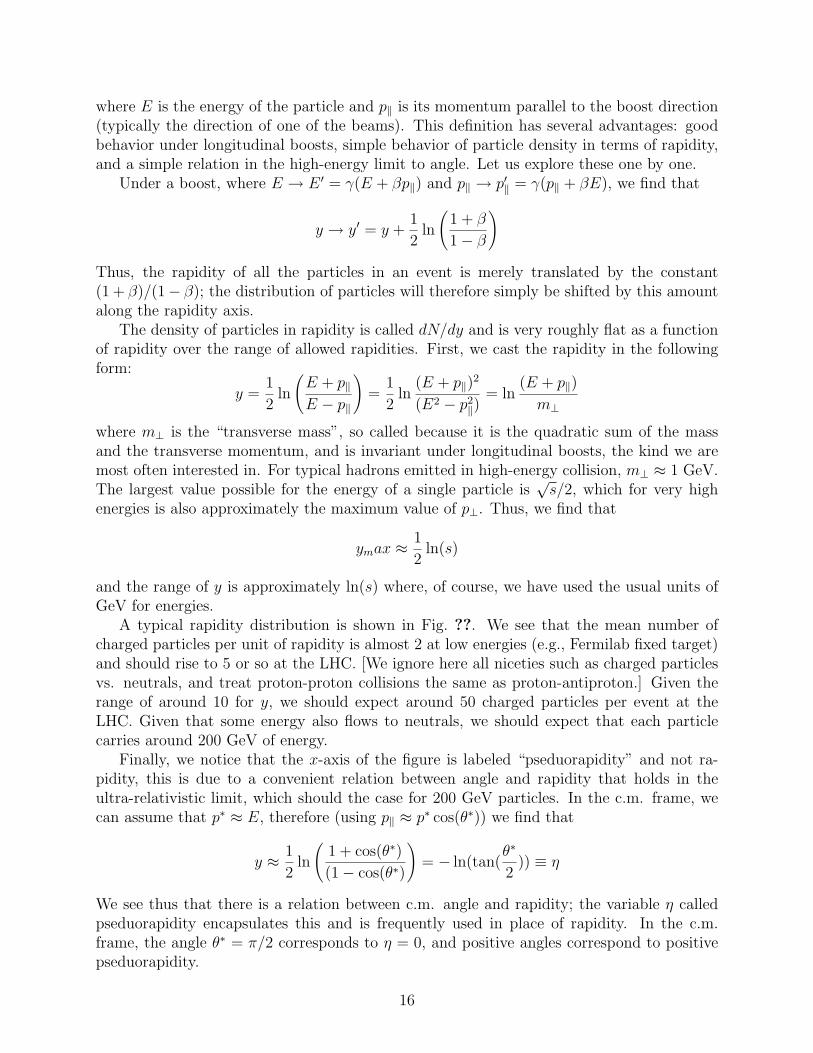
where E is the energy of the particle and p‖ is its momentum parallel to the boost direction(typically the direction of one of the beams). This definition has several advantages: goodbehavior under longitudinal boosts, simple behavior of particle density in terms of rapidity,and a simple relation in the high-energy limit to angle. Let us explore these one by one.

Under a boost, where E → E ′ = γ(E + βp‖) and p‖ → p′‖ = γ(p‖ + βE), we find that

y → y′ = y +1

2ln

(1 + β

1− β

)

Thus, the rapidity of all the particles in an event is merely translated by the constant(1 + β)/(1− β); the distribution of particles will therefore simply be shifted by this amountalong the rapidity axis.

The density of particles in rapidity is called dN/dy and is very roughly flat as a functionof rapidity over the range of allowed rapidities. First, we cast the rapidity in the followingform:

y =1

2ln

(E + p‖E − p‖

)=

1

2ln

(E + p‖)2

(E2 − p2‖)

= ln(E + p‖)

m⊥

where m⊥ is the “transverse mass”, so called because it is the quadratic sum of the massand the transverse momentum, and is invariant under longitudinal boosts, the kind we aremost often interested in. For typical hadrons emitted in high-energy collision, m⊥ ≈ 1 GeV.The largest value possible for the energy of a single particle is

√s/2, which for very high

energies is also approximately the maximum value of p⊥. Thus, we find that

ymax ≈ 1

2ln(s)

and the range of y is approximately ln(s) where, of course, we have used the usual units ofGeV for energies.

A typical rapidity distribution is shown in Fig. ??. We see that the mean number ofcharged particles per unit of rapidity is almost 2 at low energies (e.g., Fermilab fixed target)and should rise to 5 or so at the LHC. [We ignore here all niceties such as charged particlesvs. neutrals, and treat proton-proton collisions the same as proton-antiproton.] Given therange of around 10 for y, we should expect around 50 charged particles per event at theLHC. Given that some energy also flows to neutrals, we should expect that each particlecarries around 200 GeV of energy.

Finally, we notice that the x-axis of the figure is labeled “pseduorapidity” and not ra-pidity, this is due to a convenient relation between angle and rapidity that holds in theultra-relativistic limit, which should the case for 200 GeV particles. In the c.m. frame, wecan assume that p∗ ≈ E, therefore (using p‖ ≈ p∗ cos(θ∗)) we find that

y ≈ 1

2ln

(1 + cos(θ∗)

(1− cos(θ∗)

)= − ln(tan(

θ∗

2)) ≡ η

We see thus that there is a relation between c.m. angle and rapidity; the variable η calledpseduorapidity encapsulates this and is frequently used in place of rapidity. In the c.m.frame, the angle θ∗ = π/2 corresponds to η = 0, and positive angles correspond to positivepseduorapidity.

16

14 *The Electromagnetic Field Tensor

We remind readers that one of the great achievements of special relativity was to cementthe integration of electric and magnetic fields first introduced by Maxwell. Indeed, relativityhas helped us see these two fields as one and the same thing, fields which can be tansformedinto one another via Lorentz transformations. In a properly covariant description of electro-dynamics the fields are replaced with the electromagnetic field tensor F µν which is definedin terms of the 4-potential Aµ = (V, ~A) by the relation

F µν ≡ ∂µAν − ∂νAµ (61)

Recalling that the derivative ∂µ = (∂t,−~∇), we can show that

F µν =

0 −Ex −Ey −Ez

Ex 0 −Bz By

Ey Bz 0 −Bx

Ez −By Bx 0

(62)

Of course, the indices may also be lowered to get

Fµν =

0 Ex Ey Ez

−Ex 0 −Bz By

−Ey Bz 0 −Bx

−Ez −By Bx 0

(63)

Using these expressions, we can derive the transformation properties of the ~E and ~B fieldsunder Lorentz transformations and show that −(1/4)FµνF

µν and εµναβF µνFαβ are Lorentzinvariants.

For now, we will focus on using F µν to obtain a covariant form of the expression for theLorentz force.

15 Covariant form for the Lorentz Force

15.1 4-Forces

The familiar form for the Lorentz force on a moving charged particle is

~F = q( ~E + ~v × ~B)

How do we generalize this expression to be covariant? While there is no “prescription”to convert non-relativistic expressions into relativistic ones, we can be guided by the require-ments of covariance (the equation must have the same form in all frames of reference) andcorrespondence to the known expression in the non-relativistic limit.

The first thing we will do however, is to jettison the left hand side, since the entire conceptof force is mired in conceptual problems. [10] Instead, let’s use d~p/dt as a substitute, sincemomentum is a well-defined quantity that can easily be generalized to spacetime. It seemsnatural then to replace d~p/dt with dpµ/dτ (since the proper time τ is a Lorentz scalar) and

17

try to find expressions for the right hand side which are linear in the electromagnetic fieldand in the velocity, and yield the correct expression in the non-relativistic limit. Althoughseveral terms can be tried, we will display only the accepted covariant result

dpµ

dτ= qF µνvν

Let us first verify that this equation reduces to the well-known Lorentz Force Law (??)in the non-relativistic limit. Recalling that

dpµ

dτ= γ

dpµ

dt

and that vν = γ(1,−~v), we quickly see that the spatial components of this equation are

d~p

dt= q( ~E + ~v × ~B).

Thus, the Lorentz force equation holds even for relativistic motion, and is frequently appliedto describe the path of high-energy particles in magnetic fields. Consider a charged particlein a region of uniform magnetic field alone, with no electric field present, and assume furtherthat the magnetic field is perpendicular to the particle’s velocity. The time component ofequation 15.1 tells us that

dEnergy

dτ= q~v · ~E,

implying that in the absence of an electric field the particle’s energy (and hence the magni-tude of its momentum) does not change. The magnetic field merely changes the directionof the particle, which describes circles around the magnetic field lines. If the particle hasan initial momentum component along the magnetic field direction it will describe a helicalpath around the field direction with the parallel component of momentum unchanged by thefield. Since |~p| does not change with time, we may write

d~p⊥dt

= p⊥ω = qvB

where ω is the angular velocity of revolution around the field direction. If the motion of theparticle is entirely in a plane perpendicular to ~B and the radius of the circle of revolution isR, we know that v = ωR and we get finally

ω =qvB

p=

qvB

mγv=

qB

mγ

This angular velocity is often called the “cyclotron frequency”, ωc.

16 The Action Principle

We showed that the equations of motion for a free particle can be derived from the action Swhere

S =∫

dt L =∫ ∫ ∫ ∫

d4xL (64)

18

and L is the Lagrangian and L is the Lagrangian density. For a free particle, L is simplygiven by

L =mηµνv

µvν

2=

m

2(65)

Varying this action with respect to the path of the particle gives the free particle equationof motion

d2xµ

dτ 2= 0 (66)

Similary, the Langrangian density for an electromagnetic field is given by

L = −1

4FµνF

µν − jµAµ (67)

Once again, invoking the usual Euler-Lagrange equations yields the non-trivial Maxwell’sequations (2) and (3):

∂µFµν = jν (68)

Finally, combining Lagrangian densities, we can write the following expression for L for aparticle of charge q in an electromagnetic field:

L = −1

4FµνF

µν − jµAµ +

m

2(ηµνv

µvν) (69)

to get once again the equation of motion (??) for a particle of charge q in an electromagneticfield.

17 *The Spin Vector

17.1 Introduction

We can generalize the spin vector ~S to a spin 4-vector Sµ. In the particle rest frame, whereit makes sense to talk of the non-relativistic concept of “quantization direction,” we expectthat

Sµ = (0, ~S) (70)

This means thatSµS

µ = −~S2 (71)

In a frame in which the particle is moving with velocity ~β,

Sµ = [γ(~β · ~S), ~S +γ(~β · ~S)

1 + 1/γ~β] (72)

Clearly, this vector changes from the non-relativistic form in Eq. 70 to the extremerelativistic form

Sµ = (~β · ~S)(γ, γ~β) = (~β · ~S)vµ (73)

as β → 1. This extreme relativistic form can be written as

Sµ = hvµ (74)

19

where vµ is the 4-velocity and h is the component of the spin along ~β (known as the“helicity”). Notice that now Sµ is proportional to the momentum 4-vector and that

SµSµ = h2 (75)

Equation (71) for massive particles no longer holds. We see immediately that for amassless particle, which always travels at the speed of light, h2 must be a Lorentz-invariantquantity. If we call S the “spin” of the particle then Equations (73) and (74) imply thath = ±S are the only allowed values for the helicity h, i.e., all the usual (2S+1) values forthe spin are no longer allowed, only +S and −S are allowed.

17.2 The BMT equation

Next, we derive the Bargmann-Michel-Telegdi equation [1]. As with the Lorentz force law,we use as a model the non-relativistic equation

d~S

dt= ~µ× ~B

Since ~µ in turn is proportional to ~S, we seek an equation for the time derivative of ~S thatis linear in the fields, and in S. We should also be mindful of the fact that we cannot contractthe anti-symmetric tensor F µν with symmetric tensors such as vµvν or SµSν . Similarly, wecannot use terms involving pµSµ since that is zero, easily verified in the rest frame of theparticle. Thus, we are forced to consider the equation

As motivation, we recall that the right hand side

dSµ

dτ= aF µνSν + bvµvνFνσS

σ (76)

The constants a and b can be determined by contracting with pµ and by requiring thatthe equation reduces to the NR form ?? in the rest frame of the particle.

We find that a = qg/2m and b = q(g−2)/2m and obtain the “Bargmann-Michel-Telegdi”equation

dSµ

dτ=(

q

m

)(g

2

)F µνSν +

(g − 2

2

)vµvνFνσS

σ

(77)

Let us study the consequences of this equation for g = 2 and for g 6= 2, a situation calledthe “gyromagnetic anomaly”, with the “anomalous excess” of g over the nominal value of 2often being called “a”. We will see that for g = 2 the spin precesses with the momentumin a magnetic field, while the gyromagnetic anomaly drives the extra precession of the spin.This fact is used to measure the anomaly; the muon (g − 2) experiment is described.

20

18 References

References

[1] V. Bargmann, L. Michel, V. L. Telegdi, Phys. Rev. Lett. 2, 435 (1959).

[2] “Classical Electrodynamics” by J. D. Jackson, Wiley (1998).

[3] “A Unified Grand Tour of Theoretical Physics” by Ian D. Lawrie, Institute of PhysicsPublishing; 2nd edition (2001).

[4] “The Classical Theory of Fields : Volume 2” (Course of Theoretical Physics Series) byE. M. Lifshitz and L. D. Landau, Butterworth-Heinemann, 4th Edition (1980).

[5] “Theoretical Concepts in Physics: An Alternative View of Theoretical Reasoning inPhysics” by Malcolm S. Longair, Cambridge University Press, 2nd Edition, 2003.

[6] “The Special Theory of Relativity” (Nature-Macmillan physics series) by H Muirhead,Macmillan (1973).

[7] “Subtle is the Lord ...”, A. Pais, Oxford University Press (1982).

[8] S. Eidelman et al., Physics Letters B592, 1 (2004). [Particle Data Book].

[9] “Understanding Relativity: A Simplified Approach to Einstein’s Theories” by Leo Sar-tori, University of California Press (1996).

[10] See, e.g., discussions by F. Wilczek on forces in “Physics Today”, Oct. and Dec. 2004.

21