special chapters on arti cial intelligencecgatu/csia/res/lecture-06.pdf · special chapters on arti...
TRANSCRIPT

Special Chapters on Artificial IntelligenceLecture 6. Regression variable selection
Cristian Gatu
1Faculty of Computer Science“Alexandru Ioan Cuza” University of Iasi, Romania
MCO, 2018–2019
Content
Variable selection
Effects of deleting variables
Variable selection proceduresForward SelectionBackward SelectionStepwise Selection
Variable selection
I In many regression problems there will be:
1. A fixed sample size to work with.
2. A moderate to large number of potential predictorvariables.
I Generally adding more variables to a regression modelthat already contains a small number of variables willimprove predictive accuracy.
I Continuing to add variables (without adding moresample) will often lead to a deterioration in predictiveaccuracy (over-fitting).
I The goal is to find the best subset of variables:Bias/Variance trade-off.
Variable selection
I There are likely many subsets of variables that are likelyto do well.
I Finding the best subset of variables is often referred asvariable selection.
I For experiments variable selection is done before datacollection as important variables are chosen for studybased on theoretical aspects.
I For observational studies there is little control of howdata is collected. In this case variable selection is doneafter date collection and in the data analysis domain.
Content
Variable selection
Effects of deleting variables
Variable selection proceduresForward SelectionBackward SelectionStepwise Selection
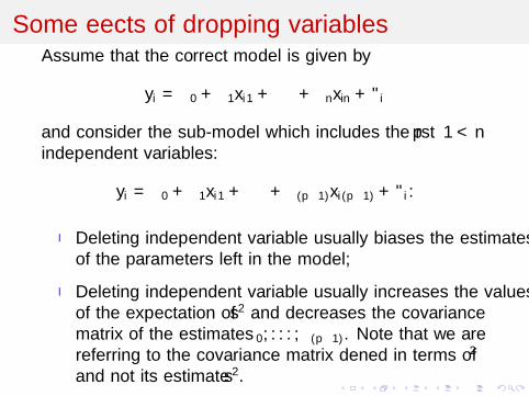
Some effects of dropping variablesAssume that the correct model is given by
yi = β0 + β1xi1 + · · · + βnxin + εi
and consider the sub-model which includes the first p − 1 < nindependent variables:
yi = β0 + β1xi1 + · · · + β(p−1)xi(p−1) + εi .
I Deleting independent variable usually biases the estimatesof the parameters left in the model;
I Deleting independent variable usually increases the valuesof the expectation of s2 and decreases the covariancematrix of the estimates β0, . . . , β(p−1). Note that we arereferring to the covariance matrix defined in terms of σ2
and not its estimate s2.
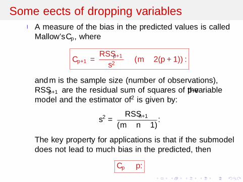
Some effects of dropping variablesI A measure of the bias in the predicted values is called
Mallow’s Cp, where
Cp+1 =RSSp+1
s2− (m − 2(p + 1)).
and m is the sample size (number of observations),RSSp+1 are the residual sum of squares of the p-variablemodel and the estimator of σ2 is given by:
s2 =RSSn+1
(m − n − 1).
The key property for applications is that if the submodeldoes not lead to much bias in the predicted, then
Cp ≈ p.
Some effects of dropping variables
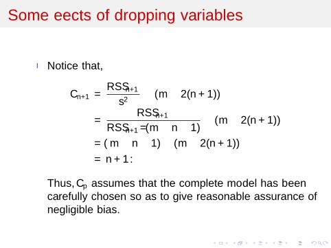
I Notice that,
Cn+1 =RSSn+1
s2− (m − 2(n + 1))
=RSSn+1
RSSn+1/(m − n − 1)− (m − 2(n + 1))
= (m − n − 1) − (m − 2(n + 1))
= n + 1.
Thus, Cp assumes that the complete model has beencarefully chosen so as to give reasonable assurance ofnegligible bias.
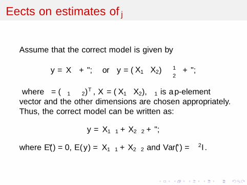
Effects on estimates of βj
Assume that the correct model is given by
y = Xβ + ε, or y = (X1 X2)(β1β2
)+ ε,
where β = (β1 β2)T , X = (X1 X2), β1 is a p-elementvector and the other dimensions are chosen appropriately.Thus, the correct model can be written as:
y = X1β1 + X2β2 + ε,
where E(ε) = 0, E(y) = X1β1 + X2β2 and Var(ε) = σ2I .
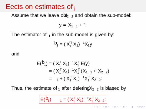
Effects on estimates of βjAssume that we leave out X2β2 and obtain the sub-model:
y = X1β1 + ε.
The estimator of β1 in the sub-model is given by:
β1 = (XT1 X1)−1X1y
and
E(β1) = (XT1 X1)−1XT
1 E(y)
= (XT1 X1)−1XT
1 (X1β1 + X2β2)
= β1 + (XT1 X1)−1XT
1 X2β2.
Thus, the estimate of β1 after deleting X2β2 is biased by
E(β1) − β1 = (XT1 X1)−1XT
1 X2β2.
Effects on estimates of βj
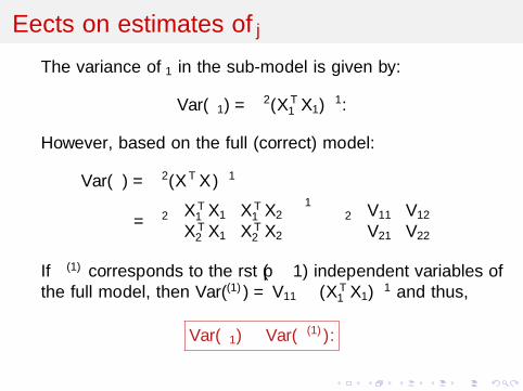
The variance of β1 in the sub-model is given by:
Var(β1) = σ2(XT1 X1)−1.
However, based on the full (correct) model:
Var(β) = σ2(XTX )−1
= σ2
(XT
1 X1 XT1 X2
XT2 X1 XT
2 X2
)−1
≡ σ2
(V11 V12
V21 V22
)If β(1) corresponds to the first (p − 1) independent variables ofthe full model, then Var(β(1)) = V11 ≥ (XT
1 X1)−1 and thus,
Var(β1) ≤ Var(β(1)).
Content
Variable selection
Effects of deleting variables
Variable selection proceduresForward SelectionBackward SelectionStepwise Selection
Variable selection procedures
When presented with a data set containing a large number ofpotential regressors, it can be a formidable task to identify auseful, well fitting and parsimonious regression model. In the1950s and 1960s statisticians spent a lot of time inventingingenious ways of automating variable selection in multiplelinear regression. The four most popular methods are forwardselection, backward selection, stepwise regression and bestsubset regression.
Variable selection procedures
The idea of the first three is to reduce the number of possiblemodels that need to be fitted. Often these methods do notprovide the same models which in most cases are not theoptimal ones1. The fourth procedure generates the bestone-regressor model, the best two-regressor model, the bestthree-regressor model etc. The best of these generated modelis selected based on some criteria (R2, adjusted R2, Cp, etc).Often an exhaustive search (considers all possible submodels)is used for generating all subset models.
1Optimal in the sense that there are better models to be selectedusing the same selection criteria
Content
Variable selection
Effects of deleting variables
Variable selection proceduresForward SelectionBackward SelectionStepwise Selection
Forward Selection
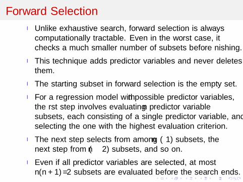
I Unlike exhaustive search, forward selection is alwayscomputationally tractable. Even in the worst case, itchecks a much smaller number of subsets before finishing.
I This technique adds predictor variables and never deletesthem.
I The starting subset in forward selection is the empty set.
I For a regression model with n possible predictor variables,the first step involves evaluating n predictor variablesubsets, each consisting of a single predictor variable, andselecting the one with the highest evaluation criterion.
I The next step selects from among (n − 1) subsets, thenext step from (n − 2) subsets, and so on.
I Even if all predictor variables are selected, at mostn(n + 1)/2 subsets are evaluated before the search ends.
Forward Selection
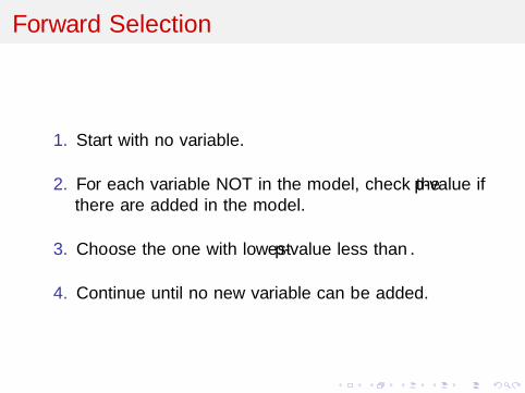
1. Start with no variable.
2. For each variable NOT in the model, check the p-value ifthere are added in the model.
3. Choose the one with lowest p-value less than α.
4. Continue until no new variable can be added.
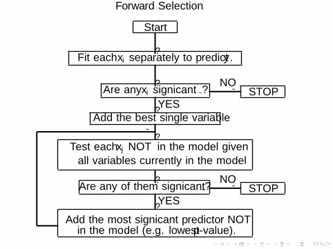
Forward Selection
Start
Fit each xi separately to predict y .
Are any xi significant ? STOP
Add the best single variable
Test each xj NOT in the model given
all variables currently in the model
Are any of them significant ? STOP
Add the most significant predictor NOTin the model (e.g. lowest p-value).
?
?
?
NO-
YES
?
? NO-
YES?
-
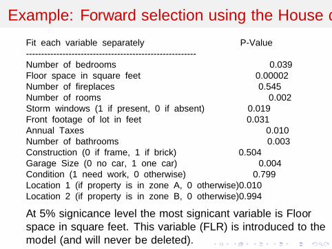
Example: Forward selection using the House data
Fit each variable separately P-Value
--------------------------------------------------------
Number of bedrooms 0.039
Floor space in square feet 0.00002
Number of fireplaces 0.545
Number of rooms 0.002
Storm windows (1 if present, 0 if absent) 0.019
Front footage of lot in feet 0.031
Annual Taxes 0.010
Number of bathrooms 0.003
Construction (0 if frame, 1 if brick) 0.504
Garage Size (0 no car, 1 one car) 0.004
Condition (1 need work, 0 otherwise) 0.799
Location 1 (if property is in zone A, 0 otherwise)0.010
Location 2 (if property is in zone B, 0 otherwise)0.994
At 5% significance level the most significant variable is Floorspace in square feet. This variable (FLR) is introduced to themodel (and will never be deleted).
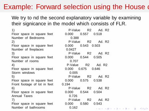
Example: Forward selection using the House data
We try to find the second explanatory variable by examiningtheir significance in the model which consists of FLR.1) P-Value R2 Ad. R2
Floor space in square feet 0.000 0.557 0.518
Number of Bedrooms 0.388
2) P-Value R2 Ad. R2
Floor space in square feet 0.000 0.543 0.503
Number of fireplaces 0.0427
3) P-Value R2 Ad. R2
Floor space in square feet 0.000 0.544 0.505
Number of rooms 0.707
4) P-Value R2 Ad. R2
Floor space in square feet 0.000 0.675 0.646
Storm windows 0.005
5) P-Value R2 Ad. R2
Floor space in square feet 0.000 0.575 0.538
Front footage of lot in feet 0.194
6) P-Value R2 Ad. R2
Floor space in square feet 0.000 0.544 0.504
Annual Taxes 0.726
7) P-Value R2 Ad. R2
Floor space in square feet 0.000 0.580 0.543
Number of bathrooms 0.162
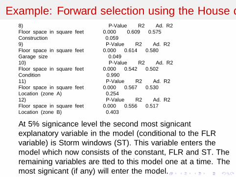
Example: Forward selection using the House data8) P-Value R2 Ad. R2
Floor space in square feet 0.000 0.609 0.575
Construction 0.059
9) P-Value R2 Ad. R2
Floor space in square feet 0.000 0.614 0.580
Garage size 0.049
10) P-Value R2 Ad. R2
Floor space in square feet 0.000 0.542 0.502
Condition 0.990
11) P-Value R2 Ad. R2
Floor space in square feet 0.000 0.567 0.530
Location (zone A) 0.254
12) P-Value R2 Ad. R2
Floor space in square feet 0.000 0.556 0.517
Location (zone B) 0.403
At 5% significance level the second most significantexplanatory variable in the model (conditional to the FLRvariable) is Storm windows (ST). This variable enters themodel which now consists of the constant, FLR and ST. Theremaining variables are fitted to this model one at a time. Themost significant (if any) will enter the model.
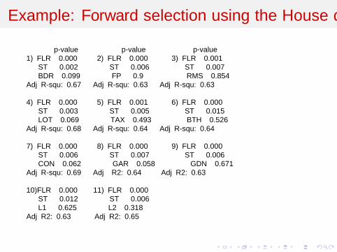
Example: Forward selection using the House data
p-value p-value p-value
1) FLR 0.000 2) FLR 0.000 3) FLR 0.001
ST 0.002 ST 0.006 ST 0.007
BDR 0.099 FP 0.9 RMS 0.854
Adj R-squ: 0.67 Adj R-squ: 0.63 Adj R-squ: 0.63
4) FLR 0.000 5) FLR 0.001 6) FLR 0.000
ST 0.003 ST 0.005 ST 0.015
LOT 0.069 TAX 0.493 BTH 0.526
Adj R-squ: 0.68 Adj R-squ: 0.64 Adj R-squ: 0.64
7) FLR 0.000 8) FLR 0.000 9) FLR 0.000
ST 0.006 ST 0.007 ST 0.006
CON 0.062 GAR 0.058 GDN 0.671
Adj R-squ: 0.69 Adj R2: 0.64 Adj R2: 0.63
10)FLR 0.000 11) FLR 0.000
ST 0.012 ST 0.006
L1 0.625 L2 0.318
Adj R2: 0.63 Adj R2: 0.65
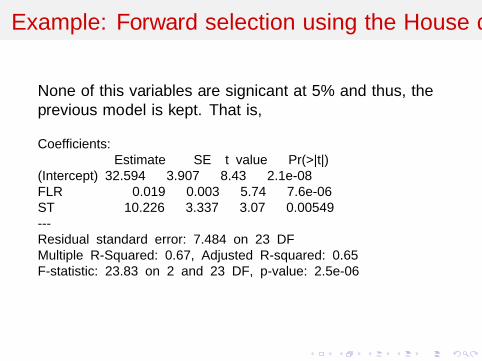
Example: Forward selection using the House data
None of this variables are significant at 5% and thus, theprevious model is kept. That is,
Coefficients:
Estimate SE t value Pr(>|t|)
(Intercept) 32.594 3.907 8.43 2.1e-08
FLR 0.019 0.003 5.74 7.6e-06
ST 10.226 3.337 3.07 0.00549
---
Residual standard error: 7.484 on 23 DF
Multiple R-Squared: 0.67, Adjusted R-squared: 0.65
F-statistic: 23.83 on 2 and 23 DF, p-value: 2.5e-06
Content
Variable selection
Effects of deleting variables
Variable selection proceduresForward SelectionBackward SelectionStepwise Selection
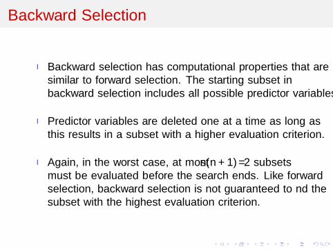
Backward Selection
I Backward selection has computational properties that aresimilar to forward selection. The starting subset inbackward selection includes all possible predictor variables.
I Predictor variables are deleted one at a time as long asthis results in a subset with a higher evaluation criterion.
I Again, in the worst case, at most n(n + 1)/2 subsetsmust be evaluated before the search ends. Like forwardselection, backward selection is not guaranteed to find thesubset with the highest evaluation criterion.
Backward Selection
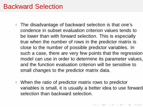
I The disadvantage of backward selection is that one’sconfidence in subset evaluation criterion values tends tobe lower than with forward selection. This is especiallytrue when the number of rows in the predictor matrix isclose to the number of possible predictor variables. Insuch a case, there are very few points that the regressionmodel can use in order to determine its parameter values,and the function evaluation criterion will be sensitive tosmall changes to the predictor matrix data.
I When the ratio of predictor matrix rows to predictorvariables is small, it is usually a better idea to use forwardselection than backward selection.
Backward Selection
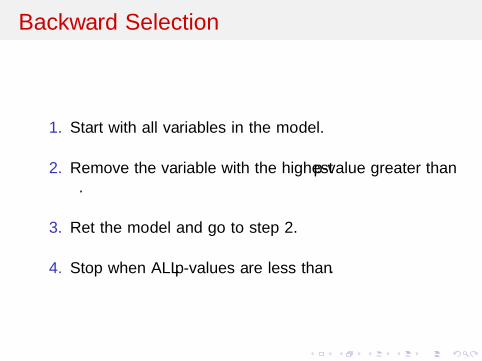
1. Start with all variables in the model.
2. Remove the variable with the highest p-value greater thanα.
3. Refit the model and go to step 2.
4. Stop when ALL p-values are less than α.
Backward Selection
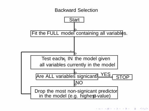
Start
Fit the FULL model containing all variables.
Test each xj IN the model given
all variables currently in the model
Are ALL variables significant ? STOP
Drop the most non-significant predictorin the model (e.g. highest p-value)
?
?
? YES-
NO?
-
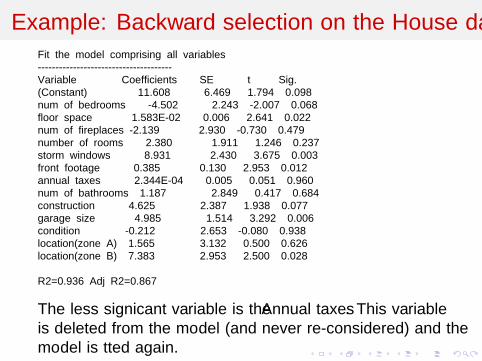
Example: Backward selection on the House dataFit the model comprising all variables
--------------------------------------
Variable Coefficients SE t Sig.
(Constant) 11.608 6.469 1.794 0.098
num of bedrooms -4.502 2.243 -2.007 0.068
floor space 1.583E-02 0.006 2.641 0.022
num of fireplaces -2.139 2.930 -0.730 0.479
number of rooms 2.380 1.911 1.246 0.237
storm windows 8.931 2.430 3.675 0.003
front footage 0.385 0.130 2.953 0.012
annual taxes 2.344E-04 0.005 0.051 0.960
num of bathrooms 1.187 2.849 0.417 0.684
construction 4.625 2.387 1.938 0.077
garage size 4.985 1.514 3.292 0.006
condition -0.212 2.653 -0.080 0.938
location(zone A) 1.565 3.132 0.500 0.626
location(zone B) 7.383 2.953 2.500 0.028
R2=0.936 Adj R2=0.867
The less significant variable is the Annual taxes. This variableis deleted from the model (and never re-considered) and themodel is fitted again.
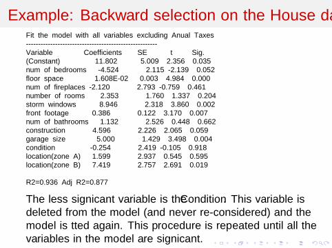
Example: Backward selection on the House dataFit the model with all variables excluding Anual Taxes
------------------------------------------------------
Variable Coefficients SE t Sig.
(Constant) 11.802 5.009 2.356 0.035
num of bedrooms -4.524 2.115 -2.139 0.052
floor space 1.608E-02 0.003 4.984 0.000
num of fireplaces -2.120 2.793 -0.759 0.461
number of rooms 2.353 1.760 1.337 0.204
storm windows 8.946 2.318 3.860 0.002
front footage 0.386 0.122 3.170 0.007
num of bathrooms 1.132 2.526 0.448 0.662
construction 4.596 2.226 2.065 0.059
garage size 5.000 1.429 3.498 0.004
condition -0.254 2.419 -0.105 0.918
location(zone A) 1.599 2.937 0.545 0.595
location(zone B) 7.419 2.757 2.691 0.019
R2=0.936 Adj R2=0.877
The less significant variable is the Condition. This variable isdeleted from the model (and never re-considered) and themodel is fitted again. This procedure is repeated until all thevariables in the model are significant.
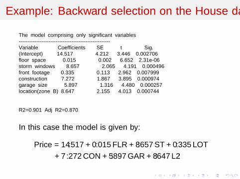
Example: Backward selection on the House data
The model comprising only significant variables
----------------------------------------------------
Variable Coefficients SE t Sig.
(Intercept) 14.517 4.212 3.446 0.002706
floor space 0.015 0.002 6.652 2.31e-06
storm windows 8.657 2.065 4.191 0.000496
front footage 0.335 0.113 2.962 0.007999
construction 7.272 1.867 3.895 0.000974
garage size 5.897 1.316 4.480 0.000257
location(zone B) 8.647 2.155 4.013 0.000744
R2=0.901 Adj R2=0.870
In this case the model is given by:
Price = 14.517 + 0.015 FLR + 8.657 ST + 0.335 LOT
+ 7.272 CON + 5.897 GAR + 8.647 L2.
Content
Variable selection
Effects of deleting variables
Variable selection proceduresForward SelectionBackward SelectionStepwise Selection
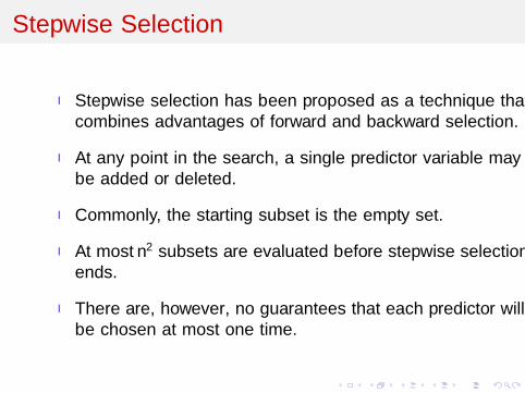
Stepwise Selection
I Stepwise selection has been proposed as a technique thatcombines advantages of forward and backward selection.
I At any point in the search, a single predictor variable maybe added or deleted.
I Commonly, the starting subset is the empty set.
I At most n2 subsets are evaluated before stepwise selectionends.
I There are, however, no guarantees that each predictor willbe chosen at most one time.
Stepwise Selection
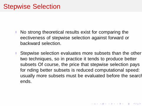
I No strong theoretical results exist for comparing theeffectiveness of stepwise selection against forward orbackward selection.
I Stepwise selection evaluates more subsets than the othertwo techniques, so in practice it tends to produce bettersubsets Of course, the price that stepwise selection paysfor finding better subsets is reduced computational speed:usually more subsets must be evaluated before the searchends.
Stepwise Selection
?
?
YES?
-NO
?
?
YES?
-NO
?
YES?
-NO
�-
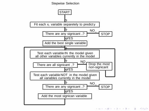
START
Fit each xi variable separetely to predict y
There are any significant ? STOP
Add the best single variable
Test each variable IN the model givenall other variables currently in the model
There are all significant ? Drop the mostnon-significant
Test each variable NOT in the model givenall variables currently in the model
There are any significant ? STOP
Add the most significan variable
Stepwise Selection
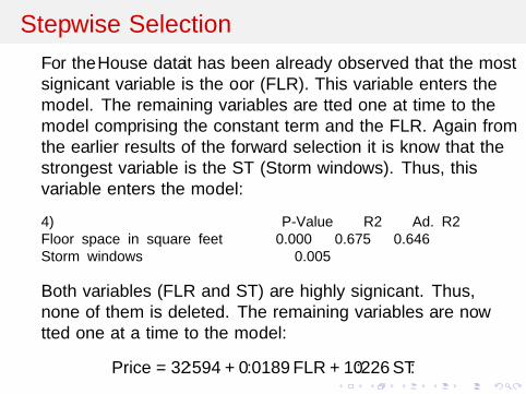
For the House data it has been already observed that the mostsignificant variable is the floor (FLR). This variable enters themodel. The remaining variables are fitted one at time to themodel comprising the constant term and the FLR. Again fromthe earlier results of the forward selection it is know that thestrongest variable is the ST (Storm windows). Thus, thisvariable enters the model:
4) P-Value R2 Ad. R2
Floor space in square feet 0.000 0.675 0.646
Storm windows 0.005
Both variables (FLR and ST) are highly significant. Thus,none of them is deleted. The remaining variables are nowfitted one at a time to the model:
Price = 32.594 + 0.0189 FLR + 10.226 ST.
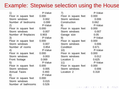
Example: Stepwise selection using the House data1) P-Value
Floor in square feet 0.000
Storm windows 0.002
Number of bedrooms 0.099
2) P-Value
Floor in square feet 0.000
Storm windows 0.007
Number of fireplaces 0.903
3) P-Value
Floor in square feet 0.000
Storm windows 0.007
Number of rooms 0.854
4) P-Value
Floor in square feet 0.000
Storm windows 0.003
Front footage 0.069
5) P-Value
Floor in square feet 0.000
Storm windows 0.005
Annual Taxes 0.493
6) P-Value
Floor in square feet 0.000
Storm windows 0.015
Number of bathrooms 0.526
7) P-Value
Floor in square feet 0.000
Storm windows 0.006
Construction 0.062
8) P-Value
Floor in square feet 0.000
Storm windows 0.007
Garage size 0.05
9) P-Value
Floor in square feet 0.000
Storm windows 0.006
Condition 0.671
10) P-Value
Floor in square feet 0.000
Storm windows 0.012
Location 1 0.625
11) P-Value
Floor in square feet 0.000
Storm windows 0.006
Location 2 0.318
Example: Stepwise selection using the House data
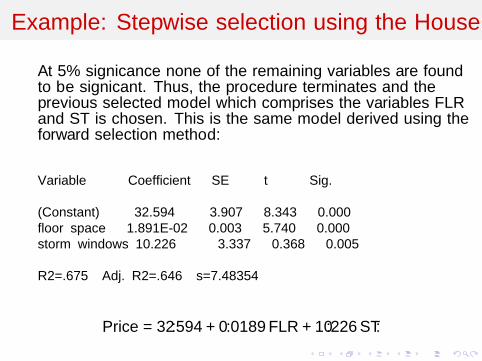
At 5% significance none of the remaining variables are foundto be significant. Thus, the procedure terminates and theprevious selected model which comprises the variables FLRand ST is chosen. This is the same model derived using theforward selection method:
Variable Coefficient SE t Sig.
(Constant) 32.594 3.907 8.343 0.000
floor space 1.891E-02 0.003 5.740 0.000
storm windows 10.226 3.337 0.368 0.005
R2=.675 Adj. R2=.646 s=7.48354
Price = 32.594 + 0.0189 FLR + 10.226 ST.