spe 71335 constraining reservoir facies models to...

Copyright 2001, Society of Petroleum Engineers Inc. This paper was prepared for presentation at the 2001 SPE Annual Technical Conference and Exhibition held in New Orleans, Louisiana, 30 September–3 October 2001. This paper was selected for presentation by an SPE Program Committee following review of information contained in an abstract submitted by the author(s). Contents of the paper, as presented, have not been reviewed by the Society of Petroleum Engineers and are subject to correction by the author(s). The material, as presented, does not necessarily reflect any position of the Society of Petroleum Engineers, its officers, or members. Papers presented at SPE meetings are subject to publication review by Editorial Committees of the Society of Petroleum Engineers. Electronic reproduction, distribution, or storage of any part of this paper for commercial purposes without the written consent of the Society of Petroleum Engineers is prohibited. Permission to reproduce in print is restricted to an abstract of not more than 300 words; illustrations may not be copied. The abstract must contain conspicuous acknowledgment of where and by whom the paper was presented. Write Librarian, SPE, P.O. Box 833836, Richardson, TX 75083-3836, U.S.A., fax 01-972-952-9435.

Abstract This paper presents a new approach to constrain reservoir facies models to dynamic data. This approach is mainly based on the combination of an optimization method called the simplex method and parameterization techniques such as the gradual deformation method.

This parameterization technique is well known for its efficiency in constraining geostatistical models to dynamic data. Originaly developped for continuous Gaussian models, the gradual deformation method was extended to facies models [12] and more recently to any kind of geostatistical model. However, the numerical behavior of the inversion can be strongly affected by discontinuities in the model changes in case of facies-based models. Our approach proposes a robust inversion method coupled with the gradual deformation method for the calibration of facies models.

The methodology we present is directly inspired by the construction of a reservoir facies model. We start by generating a related Gaussian continuous geostatistical model. In a second phase this continuous model is transformed according to the number of facies and their proportions to obtain a consistent facies model. Since a direct parameterization of the facies model does not allow the preservation of the geological properties of the model, we perform the parameterization on the related continuous model and then we proceed to the model truncation. In this manner, we can optimize the deformation parameters involved in the parameterization using the simplex method to obtain an history match.

The efficiency of this approach is illustrated by matching an interference test. The parameterization phase was

performed using the gradual deformation method. Constrained facies models were thus obtained.

A second phase of this study was devoted to quantifying the impact of uncertainty of spatial facies distribution on production forecasts. In an integrated process, we combine the simplex approach with experimental design theory and the joint modeling technique to achieve a probabilistic production forecast which takes into account the uncertainty on spatial facies distribution and classical reservoir parameters while preserving the history match. This application demonstrates the importance of the interference test matching in reducing the uncertainties on production forecasts.

Introduction The quantification of uncertainties on production forecasts is a crucial goal for taking decision in a risk prone environment. Reservoir model characterization becomes one of the most important phase in a reservoir study. All available data should be integrated into the model to provide a more realistic description of the reservoir in order to reduce uncertainties and obtain reliable production forecasts.

Geostatistical simulation is currently widely used to give a realistic reservoir description. Although geostatistics is clearly well suited to model geological information, it leads to an uncertain framework since the geostatistical model properties make it possible to produce not one geological model but a set of equiprobable realizations of the geological model.

Use of geostatistical models leads then clearly to an important problematic: the integration of available dynamic data while quantifying the uncertainty on production forecasts due to this geostatistical modeling.

The task of constraining reservoir facies models is a hard problem since it requires dealing with two main difficulties: - to find an accurate optimization method that minimizes the

objective function which represents the mismatch beetween the dynamic data and the simulated values of the pressure or of the production,

- to find an efficient parameterization method which allows to have a precise description of the facies model while keeping the number of involved parameters as small as possible to ensure a reasonable cost for the matching phase.

SPE 71335

Constraining Reservoir Facies Models to Dynamic Data - Impact of Spatial Distribution Uncertainty on Production Forecasts I. Zabalza-Mezghani, IFP, M. Mezghani, IFP, G. Blanc, IFP

2 I. ZABALZA-MEZGHANI, M. MEZGHANI, G. BLANC SPE 71335

This work presents a new approach for constraining reservoir facies model to dynamic data while quantifying the uncertainty on production forecasts. We suggest the use of the simplex method as an optimization technique since it is well suited to the particular form of the objective function, and the use of the gradual deformation method to parameterize the reservoir facies models. The quantification of uncertainty on production forecasts is performed using experimental design theory.

More precisely, we illustrate our approach with a field case, where we decide to test a water injection scheme. In an integrated process which mixes gradual deformation, simplex method, experimental design and the joint modeling method, we show that the integration of interference test data on reservoir facies models is crucial since it allows an important dicrease of the uncertainties on the expected recovery factor.

Constraining Reservoir Facies Models The objective here is to constrain a reservoir facies model to dynamic data. This consists in finding the model which best fits the dynamic data.

To find this model, a classical procedure consists in building and then minimizing an objective function which quantifies the mismatch between the simulated results and the dynamic data. Thus, the reservoir facies model is updated until finding the one that satisfies the data. This update needs to be able to describe the reservoir facies model with a few set of parameters: it is the goal of the parameterization phase.

Before presenting the parameterization we used: the gradual deformation method, we explain the main principle of a reservoir facies model simulation.

Reservoir Facies Model Simulation. The simulation of a reservoir facies model relies on the simulation of a gaussian white noise. Thus, this white noise is transformed in categories or facies according to a given variogram, a number of facies, facies volume fractions, correlation lengths to obtain a reservoir facies model. Facies models can be obtained using either truncated Gaussian simulations [13] or sequential indicator simulation [14]. In both cases, the gradual deformation method must be performed on the Gaussian white noise, before the transformation. As an example, we illustrate on figure 1 the principle of the truncated Gaussian simulation.

The parameterization:The Gradual Deformation Method. The basic principle of the gradual deformation [4][9][10] method is to generate a process of realizations which evolve smoothly at each step. This can be achieved by introducing a correlation between a new realization and the realization obtained at the previous step.

To apply this principle to continuous geostatistical models, the gradual deformation method propose to generate new realizations as linear combinations of any number of independent initial realizations. Then, if we note {Z1, …, Zn} a set of n independent realizations of a Gaussian random field, a new realization can be expressed as follows:

∑=

=n

i

iiZZ1

α ....................................................................... (1)

where { }nαα ,,1… are n real coefficients between –1 and 1. The geostatistical structure of the model (variogram,

correlation strength, …) is conserved through this linear expression. Moreover, the variance model is unchanged under the following condition:

∑=

=n

i

i

1

2 1α .......................................................................... (2)

A new formulation of equation (1), which takes into account this constraint is:

( ) ( ) ( )∏ ∑ ∏−

=

−

=

−

+=

++=1

1

1

1

1

1

11 cossincosn

i

n

i

n

ij

ijii ZZZ πρπρπρ ................... (3)

As shown in equation (3), the new realization Z can be defined through the set of parameters { }11 ,, −nρρ … .

This parameterization is well-suited for constraining continuous geostatistical models [4]. But it can not be applied directly to facies models, since the categories can not be combined in a consistent way.

To remove this difficulty, L.Y. Hu [12] suggest to apply the gradual deformation method not on the facies model, but on the related gaussian white noise which is involved in the simulation process (figure 1). In this way, we are able to control the facies realizations through a reduced number of parameters { }11 ,, −nρρ … , while preserving the consistency of the resulting reservoir facies models. The optimization Process. An objective function can be defined to assess the match of the dynamic data. We use a least squares formulation which quantifies the errors between the simulation results and the observed data:

( )∑=

−=obsn

i

obsi

simii ddwF

1

2

21 ..................................................... (4)

where dsim are the simulated production results, dobs are the dynamic data, w are weighting coefficients (to traduce the confidence in the data), and nobs is the number of measurements to match.

Deforming the facies model, in updating the parameters { }11 ,, −nρρ … , will change the simulated production results dsim and then the objective function. In this way, the objective function depends on the deformation parameters { }11 ,, −nρρ … , and our goal is to find a set of { }11 ,, −nρρ … which minimizes the objective function, that is to find a reservoir facies model which honors the dynamic data.

The transformation in categories phase in the facies model simulation (figure 3) leads to a non differentiability of the objective function. This specific behavior, due to facies models, forbid the use of classical non-linear optimization algorithm, like Gauss-Newton or Steepest Descent, since they require gradient computation which is not possible in our

CONSTRAINING RESERVOIR FACIES MODELS TO DYNAMIC DATA - IMPACT OF SPATIAL SPE 71335 DISTRIBUTION UNCERTAINTY ON PRODUCTION FORECASTS 3

framework. To bypass this problem, we suggest the use of an optimization algorithm which is based on direct evaluation of the objective function only, without gradient computation. To keep in mind one of our goal: the quantification of uncertainties, we have decided to use an optimization approach which relies on experimental designs: the simplex method.

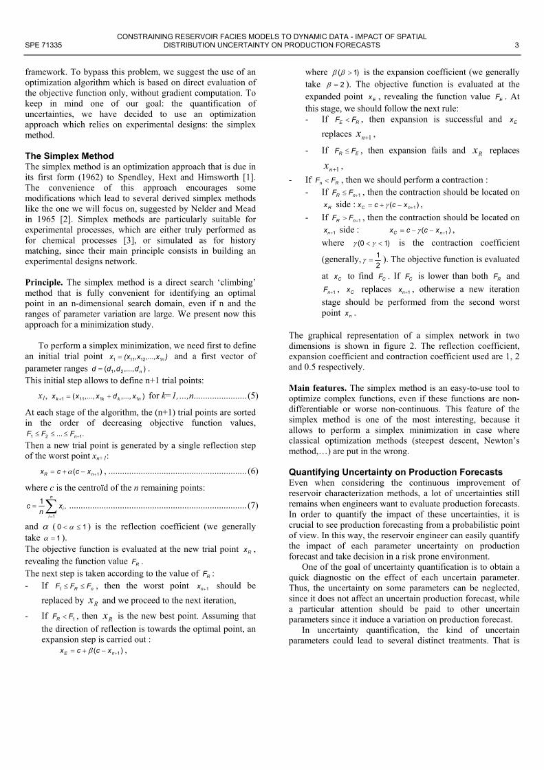
The Simplex Method The simplex method is an optimization approach that is due in its first form (1962) to Spendley, Hext and Himsworth [1]. The convenience of this approach encourages some modifications which lead to several derived simplex methods like the one we will focus on, suggested by Nelder and Mead in 1965 [2]. Simplex methods are particularly suitable for experimental processes, which are either truly performed as for chemical processes [3], or simulated as for history matching, since their main principle consists in building an experimental designs network. Principle. The simplex method is a direct search ‘climbing’ method that is fully convenient for identifying an optimal point in an n-dimensional search domain, even if n and the ranges of parameter variation are large. We present now this approach for a minimization study.

To perform a simplex minimization, we need first to define

an initial trial point ),...,x,x(xx n112111 = and a first vector of parameter ranges ),...,,( 21 ndddd = . This initial step allows to define n+1 trial points:

x1, ),...,,...,( 11111 nkkk xdxxx +=+ for k=1,…,n....................... (5)

At each stage of the algorithm, the (n+1) trial points are sorted in the order of decreasing objective function values,

.... 121 +≤≤≤ nFFF Then a new trial point is generated by a single reflection step of the worst point xn+1:

)( 1+−+= nR xccx α , ............................................................ (6)

where c is the centroïd of the n remaining points:

,1

1∑

=

=n

i

ixnc ............................................................................. (7)

and α ( 10 ≤< α ) is the reflection coefficient (we generally take 1=α ). The objective function is evaluated at the new trial point Rx , revealing the function value RF . The next step is taken according to the value of RF : - If nR FFF ≤≤1 , then the worst point 1+nx should be

replaced by Rx and we proceed to the next iteration,

- If 1FFR < , then Rx is the new best point. Assuming that the direction of reflection is towards the optimal point, an expansion step is carried out : )( 1+−+= nE xccx β ,

where )1( >ββ is the expansion coefficient (we generally take 2=β ). The objective function is evaluated at the expanded point Ex , revealing the function value EF . At this stage, we should follow the next rule: - If RE FF < , then expansion is successful and Ex

replaces 1+nx ,

- If ER FF ≤ , then expansion fails and Rx replaces

1+nx , - If Rn FF < , then we should perform a contraction :

- If 1+≤ nR FF , then the contraction should be located on Rx side : )( 1+−+= nC xccx γ ,

- If 1+> nR FF , then the contraction should be located on 1+nx side : )( 1+−−= nC xccx γ ,

where )10( << γγ is the contraction coefficient

(generally,21

=γ ). The objective function is evaluated

at Cx to find CF . If CF is lower than both RF and 1+nF , Cx replaces 1+nx , otherwise a new iteration

stage should be performed from the second worst point nx .

The graphical representation of a simplex network in two dimensions is shown in figure 2. The reflection coefficient, expansion coefficient and contraction coefficient used are 1, 2 and 0.5 respectively.

Main features. The simplex method is an easy-to-use tool to optimize complex functions, even if these functions are non-differentiable or worse non-continuous. This feature of the simplex method is one of the most interesting, because it allows to perform a simplex minimization in case where classical optimization methods (steepest descent, Newton’s method,…) are put in the wrong.

Quantifying Uncertainty on Production Forecasts Even when considering the continuous improvement of reservoir characterization methods, a lot of uncertainties still remains when engineers want to evaluate production forecasts. In order to quantify the impact of these uncertainties, it is crucial to see production forecasting from a probabilistic point of view. In this way, the reservoir engineer can easily quantify the impact of each parameter uncertainty on production forecast and take decision in a risk prone environment.

One of the goal of uncertainty quantification is to obtain a quick diagnostic on the effect of each uncertain parameter. Thus, the uncertainty on some parameters can be neglected, since it does not affect an uncertain production forecast, while a particular attention should be paid to other uncertain parameters since it induce a variation on production forecast.

In uncertainty quantification, the kind of uncertain parameters could lead to several distinct treatments. That is


why we describe quickly the main kind of parameters involved in a reservoir study.

Uncertain Parameter Description. The first step of an uncertainty quantification (or a risk analysis) consists in listing the possible uncertain parameters whitout any a priori, and then fixing a range of uncertainty for each listed parameter.

In most of reservoir studies, one can distinguish three kinds of uncertain parameters: - "Physical parameters" which are an integral part of the

reservoir, but remain uncertain because of the bad knownledge of the field. Typically, they can be permeabilities, porosities, saturations, facies volume fractions, correlation lengths, … These "Physical parameters" are uncontrolled by engineers, but they have no random effect on production (production is directly correlated with parameter variations).

- "Production parameters" which are involved in the production scheme devlopment. Typically, they can be the perforated length of wells, the flowrates, the well locations, … These "Production parameters" have no random effect on production too, but we should distinguish them form "Physical parameters" since they are controlled by engineers and would thus be optimized to better fit a high production goal.

- "Stochastic parameters" which group together all uncertainties which have a random effect (non smooth) on production. Typically, they can be several geostatistical models with the same properties (only the seed differs), several possible structural maps, several possible fracture networks … This kind of uncertainty will affect the production non-continuously, which require a specific approach to quantify the related uncertainty.

These three kinds of uncertainty can be handle using experimental design theory, but a specific method shall be applied for quantifying "Stochastic Parameters" uncertainty: the Joint Modeling Method [5][7][11]. In the field case study that we present, we consider uncertainties on "physical parameters", such as waterflood residual oil saturation, relative permeability Corey coefficients, …, but also on "stochastic parameters" since we will quantify the impact of the facies spatial distribution uncertainty on a production response (the cumulative oil). In this field case, we show that the integration of an interference test data in a matching phase allowed to reduce the uncertainty on the expected cumulative oil. Experimental Design. This theory [8] allows to study and quantify the impact of uncertain parameters on a given process.

Let us consider a production response of interest, (typically, the cumulative oil production, the recovery factor, the gas-oil ratio), denoted by y, and some uncertain reservoir parameters which can be "Physical parameters" or "Production parameters", denoted by x1, x2, …, xn .

The experimental design theory provides the right set of reservoir simulations to perform to understand the behavior of y as a function of the uncertain parameters x1, x2, …, xn .

Especially, it allows to: - identify the parameters that are actually influent on the

production response y. This step is crucial since it allows to eliminate parameters that have a negligeable impact on the response and to focus on the influent ones.

- build a regression model which links the production response y to the influent uncertain parameters.

The regression model can be seen as an accurate approximation of the production response behavior, and in this way, it quantifies safely the effect of all the uncertainties on the production response. Usually, a polynomial model is sufficient to catch the production response behavior as a function of the uncertain parameters:

2211222110 nnxxxxxy βββββ ++++++≈ …… ......................... (8)

This simple analytical model will bypass the reservoir flow simulator (for the uncertainty quantification) to provide fast evaluation of production forecasts in an uncertain environment. One of the most obvious use of the regression model is clearly the intensive computation, for Monte-Carlo sampling for instance. On the other hand, if the uncertain parameters are "Production parameters", a simple optimization of the regression model will provide the optimal production condition (well locations, flowrates …) to increase the final recovery. The Joint Modeling Method. The Joint Modeling Method [7][11] allows to quantify the impact of both "deterministic" parameters (Production and Physical parameters) and "stochastic" ones. This approach is mainly based on experimental design theory, since it requires to run a set of reservoir simulations to catch the behavior of y as a function of the "deterministic" parameters x1, x2, …, xn , but it allows to characterize the effect of having several possible facies models to describe the reservoir.

In such a case, the production response will be affected by: - the variation of the deterministic parameters (even if we

consider only one possible facies model), - the facies model changes (even if the deterministic

parameters are fixed). To catch this dual variation of the production response,

the Joint Modeling method suggests to model the production response with two regression models (coming from experimental design): - A mean model which allows to describe the production

response as a function of the deterministic parameters, - A dispersion model which allows to describe the

dispersion of the production response due to considering several possible facies models.

These two regression models are linked using specific statistical models (generalized linear models). Then an interaction effect (cumulative effect of both stochastic uncertainty and uncertainty on deterministic parameter ) on the


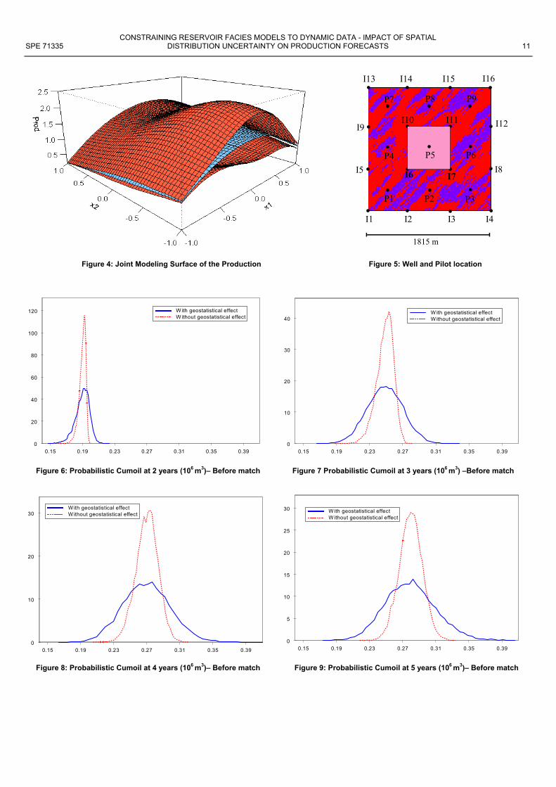
production behavior can be quantified. To illustrate the principle of this methodology, the figure 4 represents the two resulting models for 2 uncertain parameters. The blue surface located in the middle represents the mean behavior of the production as a function of the 2 uncertain parameters, and the 2 orange boundary surfaces represent the dispersion due to geostatistical modeling.

This innovative approach is essential in quantifying uncertainty on production forecasts since the effect of geostatistics is often at least as important as the effect of classical other reservoir parameters.

Field Case Study In this case study, the objective was to highligth the necessity to quantify and reduce uncertainties on production forecast in a field development before decision making.

A synthetic case was used to validate the methodology, and to prove that constraining possible geostatistical models to dynamic data is crucial to dicrease uncertainties on production forecasts. Reservoir Description. In this study we focus on a sector of the reservoir which covers a surface area of 1815 m by 1815 m. The geological model for this sector is a 3D model composed of three layers with a constant thickness of 10 m. It is discretized on a regular grid of 121×121×3 grid blocks of 15 m by 15 m by 10 m. Two distinct facies F1 and F2 are involved in this model. The facies F1 represents 35% of the facies volume and F2 represents 65%. The correlation lengths along the main anisotropy direction are respectively 500m and 100 m horizontaly, and 30 m verticaly. The main anisotropic direction is diagonal with respect to the reservoir grid.

One of the two facies is assumed to be of good reservoir quality, and the other of poorer quality. The permeability and porosity for each facies are homogeneous.

The value of the permeability k1 of the good facies F1 is uncertain, and we assume that it could belong to the following range [800 mD ; 1600 mD]. The porosity of this facies is 0.2. The permeability of the poor facies is 50 mD and its porosity is 0.05. The oil-water relative permeability was modeled using analytical curves which are fully characterized by end points and Corey coefficients. The sector production is accomplished through 16 water injector wells and 9 oil production wells regularly located, as shown on figure 5.

Problematic. The objective of this study was to present a methodology to quantify the impact of uncertainty on production forecasts, and especially to quantify uncertainty due to the geostatistical modeling.

The problematic was to test a water-injection process on the sector, to evaluate the efficiency of the recovery process. Moreover, we have focused on the quantification of the integration of interference test data to reduce the uncertainty on production forecasts.

One of the main difficulty of this feasibility study is the management of uncertainties on reservoir parameters. Then,

the goal of this study is to precisely define the production forecasts in a water-injection scenario while taking into account the fact that the values of several parameters are not well known. One of the most important question in this study is then: does the uncertainty on parameters affect the production forecasts, and if this is the case, in which range could we expect the production to vary ?

Indeed, it is as important to predict the expected value of the recovery process, as the risk which remains around this prediction, and which is due to the uncertainties on parameters.

In a first step, we have decided to test the efficiency of the water-injection process on a pilot area which is located at the center of the field. We will then assume that the behavior of this pilot is fully representative of the total field behavior. To do so, we have proceeded to a risk analysis study, which allows to quantify the impact of uncertainties on production forecasts for this pilot.

Uncertainty on Production Forecasts. The pilot area comprises a producing well P5 surrounded by four injection wells I6, I7, I10 and I11. The objective is to study the behavior of the Cumulative Oil production for P5 at 2 years, 3 years, 4 years and 5 years.

Several uncertainties on the reservoir knownledge should affect the expected recovery on the pilot: - the geostatistical modeling since several equiprobable

realizations could lead to variable production forecasts, - the petrophysical properties. Indeed, the description of some petrophysical properties is uncertain: - the permeability k1 of the good facies F1 could belong to

[800 mD ; 1600 mD], - the Sorw varies in [0.15 ; 0.25] - the end point for the water curve (Krwmax) varies in [0.4

; 0.7] - the Corey coefficient for the water curve varies in [1 ; 3], - the Corey coefficient for the oil curve varies in [3 ; 5]. To quantify the effect of these uncertainties on the behavior of the cumulative oil production, a risk analysis has been performed using experimental design theory and the Joint Modeling method.

The involved experimental design was a Central Composite Design for 5 parameters (k1, Sorw, Krwmax, CorW, CorO) which is composed of 27 distinct combinations of (k1, Sorw, Krwmax, CorW, CorO) values in their range of variation. To catch the uncertainty due to the geostatistical modeling, we have decided to run each of the 27 combinations for five distinct realizations of the geostatistical facies model.

Thus, the resulting simulated values of the production for the pilot were representative of the effect of the uncertainties on petrophysics and also on geostatistics. These simulated production results were then used in a Joint Modeling process to reach an efficient modeling of the cumulative oil production which integrates both the potential uncertainty on the petrophysical parameters and on the geostatistical modeling.


This procedure was performed for 4 times: at 2 years, 3 years, 4 years and 5 years. As an illustration, the equations (9) and (10) shows the joint models for the cumulative oil production at 3 years.

CorO0.0021CorW CorOKrwmax 0.0001 - CorWKrwmax 0.0013 CorOSorw 0.0004

- CorWSorw 0.0002 -Krwmax Sorw 0.0001- CorOk1 0.0003 CorWk1 0.0002 -Krwmax k1 0.0003-Sorw k1 0.0001

- CorO 0.0002-CorW 0.0032 -Krwmax 0.0007 Sorw 0.0004- k1 0.0005 CorO 0.0043 - CorW 0.0135 Krwmax 0.0056-Sorw 0.0058- k1 0.0036- 0.25

22 2

22

×+××+×

×××+×××

++

+≈Cumoil

(9)

CorO)CorW 0.007 CorOKrwmax 0.0055- CorWKrwmax 0.103 CorOSorw 0.005

CorWSorw 0.059Krwmax Sorw 0.034- CorOk1 0.0009 CorWk1 0.099Krwmax k1 0.033-Sorwk1 0.019

- CorO2 0.035- CorW2 0.118- Krwmax2 0.006- Sorw2 0.009- k12 0.03- CorO 0.093 CorW 0.125Krwmax 0.037

-Sorw 0.044 k1 0.026- -7.87exp(

×+××+×+

×+××+×+××

+++≈DispCumoil

(10)

The first model allows to compute at a negligible cost the

mean value of the expected cumulative oil production at 3 years for any values of (k1, Sorw, Krwmax, CorW, CorO) in their range of variation. Thus, using this model, one could perform Monte-Carlo sampling to obtain cheeply a probabilistic distribution of the cumulative oil production with respect to the deterministic parameter variations. On the figures 6, 7, 8 and 9, are represented these distribution as dotted red curves for the four years.

But the innovative concept concerns the second model, which allows to catch the cumulative oil dispersion due to the fact of dealing not only with a unique geostatistical model, but with several equiprobable ones. This model allows to compute easily the expected dispersion of the cumulative oil production (around its mean value) due to the geostatistical modeling. Thus, a Monte-Carlo sampling which involves both models will provide cheeply a probabilistic distribution of the cumulative oil production which takes into account both the effect of "classical" uncertain parameters (in this case petrophysics) and the geostatistical spatial distribution of the facies. The figures 6, 7, 8 and 9 show the resulting probabilistic distribution of the cumulative oil production for the four years on the pilot. The blue solid curves represent the probable cumulative oil production obtained with the Joint Modeling method, that is while taking into account all kinds of uncertainties (classical and geostatistical ones).

The figures show clearly that the quantification of the uncertainty on the geostatistical modeling can not be neglected since this uncertainty increases highly the range of variation of the cumulative oil production. For instance at 3 years, the cumulative oil production is expected to vary beetween: - [0.21 ; 0.27] million m3 in neglecting the geostatistical

context, - [0.18 ; 0.32] million m3 in taking into account the

geostatistical modeling.

It is obvious that taking a decision while neglecting geostatistical effects remains really risked and could re-open the question of the rentability of the project.

The figure 10 shows the variation intervals for the cumulative oil all over the 5 years of simulated production. The production forecasts are quite good, since at 3 years the expected cumulative oil is about 0.25 million m3 , which in comparison with the initial oil in place represents about 38 % of recovery.

As a conclusion to this first part of the study, it appears that a water-injection process leads to a satisfactory recovery coefficient, but an important risk remains, due to the uncertainty on both the petrophysical parameters and the geostatisical modeling. Indeed, for a recovery factor of 38% at 3 years, the uncertainty represents about 8%. This conclusion has motivated us to study the benefit of including dynamic data in order to reduce the uncertainties. A specific focus on the geostatistical model characterization was performed. Indeed, we planned to integrate interference test data to better characterize the spatial distribution of the facies model, and thus to reduce the variability due to the geostatistical modeling.

Interference Test Matching. The main objective of this phase of the study was to quantify the reduction of the geostatistical uncertainty obtained by constraining the model to dynamic data and the impact on the production. An interference test was performed on the pilot. The history of P5 comprises a period of constant production rate at 300 m3/day during 2 days, and a period of pressure buildup (zero rate) during 8 days. The four injection wells I6, I7, I10 and I11 were considered as observation wells. For numerical fluid flow simulations, the regular gridding was gradually refined locally until regular cells of 1 m were obtained around the producing well P5.

Synthetic interference test data were defined by a numerical flow simulation run based on the geostatistical reference model shown on figure 11. The resulting well test data comprise the downhole pressure evolution at the four observation wells, and the downhole pressure evolution and its derivative at the producing well P5.

Matching parameters. The permeability k1 of the good

facies F1 (which was assumed to be in [800 mD ; 1600 mD] until now) is one of the parameters involved in the matching process. Indeed, the interference test allows to reduce the uncertainty on this parameter. As an initial guess for this permeability we chose its lowest value: 800 mD.

The other parameters involved in the matching process are gradual deformation parameters, since our goal in performing an interference test is to better characterize the spatial distribution of the facies. Thus, we randomly pick 10 gaussian white noises to start the matching process, that is, according to equation 3, 9 gradual deformation parameters θi, i=1,…,9.


Matching process. The matching process is performed using the simplex method and the gradual deformation method, as shown on figure 3. The simplex method is in this study particularly efficient (in comparison with gradient based optimization techniques) since, the objective function is non-differentiable due to the truncation phase in the generation of the facies model. Thus, the simplex method, which does not require any gradient computation is in this context clearly well-suited.

To start the matching step, an initial geostatistical model was generated (figure 12). The optimization process (figure 3) was performed until finding a satisfactory match. On figures 13, 14, 15, 16 and 17, we present the result of the match for the 5 wells after 247 single phase flow simulations. The figure 18 presents the resulting optimal facies model.

To deal with the geostatistical context, we did not neglect the fact that several geostatistical realizations can honor the dynamic data. Thus, we decided to perform 4 other matching process starting at each new process with a new initial guess. At the end of this phase, we obtained 5 geostatistical facies model, and 5 values of the permeability k1 (one for each constrained model), which all allow to match the interference test data.

The next step of this study was then to quantify the impact of this matching phase on production forecasts. In other words: has the matching of the interference test data allowed to reduce the uncertainty on production forecasts ?

Reducing Uncertainties. In order to quantify the reduction of uncertainty on production forecasts, the most natural way was to perform again the risk analysis, which comprises experimental design, Joint Modeling and Monte-Carlo sampling, using the 5 geostatistical constrained facies models, and the 5 corresponding values of the permeability k1, which were provided by the matching step.

Thus, we built an experimental design for 4 parameters: - the Sorw which still varies in [0.15 ; 0.25] - Krwmax which still varies in [0.4 ; 0.7] - CorW which still varies in [1 ; 3], - CorO which still varies in [3 ; 5]. The uncertainty on the permeability k1 is no more involved through the experimental design, since it is handled by the fact of taking the 5 values of k1 provided by the matching step.

The resulting experimental design for these 4 parameters was a Central Composite Design which delivers 25 combinations of (Sorw, Krwmax, CorW, CorO). Each combination was run for the five distinct realizations provided by the matching step.

As in the first step of the study, a Joint Modeling was performed at 2, 3, 4 and 5 years of production and as an illustration the equations 11 and 12 present the resulting models for the cumulative oil production after the matching phase at 3 years:

CorO.CorW 0.0034 CorOKrwmax 0.0001 CorW Krwmax 0.001

CorOSorw .00010 CorWSorw 0.0005-Krwmax Sorw 0.0002- CorO 0.0002

CorW 0.003- Krwmax 0.001 Sorw 0.0005- CorO 0.002- CorW 0.018 Krwmax 0.009-Sorw 0.007- 0.238

2

222

×+×+×

+×+××

++

+≈Cumoil

(11)

CorO)CorW 0.154- CorOKrwmax 0.049 CorWKrwmax 0.019

CorOSrow 0.051- CorWSorw 0.007-Krwmax Sorw 0.011 CorO 0.031- CorW 0.003

- Krwmax 0.057- Sorw 0.026- CorO 0.386- CorW 0.33-Krwmax 0.251 0.057Sorw - 11.27- exp(

22

22

××+×+×××+

+≈DispCumoil

(12)

Using these two models, we can rebuild the probabilistic

distribution of the cumulative oil production at 2 years (figure 19), at 3years (figure 20), at 4 years (figure 21), at 5 years (figure 22), while taking into account the effect of the 5 geostatistical constrained models and the petrophysical uncertain parameters (blue solid curves), or while taking into account only the uncertainty on petrophysics and not on geostatistics (red dotted curves).

The important result shown on the figures is that the red dotted curves and the blue curves are now very close. In other words, the matching phase allowed to remove the uncertainty due to the geostatistical modeling.

In terms of ranges of variation of the cumulative oil production, the figure 23 shows that the matching phase has allowed to reduce significantly the uncertainty. The production forecasts are quite good, since at 3 years the expected cumulative oil is about 0.23 million m3 , which in comparison with the initial oil in place represents about 31 % of recovery. Note that the dicrease of the recovery factor is mainly due to the fact that for the constrained facies models the initial oil in place in the trap is higher (and actually closer to the reference model initial oil in place). In terms of uncertainty, the range of variation of the cumulative oil production in comparison with the initial oil in place represents about 2.7% against 8% without history matching.

Conclusions The methodology presented in this paper relies on: - an optimization process to constrain the geostatistical

facies models to dynamic data. This method involves both the simplex method, which is powerfull for constraining facies models and the gradual deformation method which allows to describe a complex geostatistical model with a small number of parameters,

- an innovative risk analysis approach, the Joint Modeling method, which allows to quantify the impact of the classical uncertain parameters (petrophysics, production parameters …), and above all the impact of the geostatistical context.


This case study illustrate clearly the necessity to take into account dynamic data in a risk analysis and especially in a geostatistical framework.

Indeed, the matching process that we have presented in this paper allowed to clearly demonstrate the impact of the spatial distribution of the facies on production forecasts, and the Joint Modeling method demonstrated its efficiency for estimating uncertainties in a geostatistical context. Acknowledgments The authors wish to thank IFP for permission to publish the results of this study. A particular thanks is devoted to Frédéric Roggero and Emmanuel Manceau for their help to built the synthetic case. Part of this work has been performed in the COUGAR consortium, which is an IFP consortium currently sponsored by BHP, ENI-AGIP, GDF, PETROBRAS, PEMEX and REPSOL-YPF. References 1- Spendley, W., Hext, G.R., Himsworth, F.R.:"Sequential

Application of Simplex Designs in Optimization and Evolutionary Operation", Technometrics, n°4, pp.441, 1962.

2- Nelder, J.A., Mead, R.:"A simplex Method for function Optimization", The computer Journal, n°7, pp.308, 1965.

3- Porte, C. , Debreuille, W. , Delacroix, A.:"La méthode simplex et ses dérivées", L'actualité chimique, October1984.

4- Roggero ,F., Hu, L.Y.:"Gradual Deformation of Continuous Geostatistical Models for History Matching", paper SPE 49004 presented at the 1998 SPE Annual Technical Conference & Exhibition, New Orleans, September 27-30.

5- Zabalza , I., Dejean, J.P., Collombier, D., Blanc, G.:"Prediction and Density Estimation of a Horizontal Well Productivity Index using Generalized Linear Models", paper B31 presented at the 1998 ECMOR VI, Peebles, September 8-11.

6- Zabalza-Mezghani , I., Blanc, G., Collombier, D., Mezghani, M.:"Use of Experimental Design in Resolving Inverse Problems – Application to History Matching", paper V1 presented at the 2000 ECMOR VII, Baveno, September 5-8.

7- Zabalza-Mezghani , I., Manceau, E., Roggero, F.:" A new approach for quantifying the impact of geostatistical uncertainty on production forecasts: the Joint Modeling Method. ", paper to be presented at the 2001 IAMG, Cancun, September 6-12.

8- Box G.E.P and Wilson K.B., "On the experimental attainment of optimum conditions", Journal of the Royal Statistical Society, Series B, 13, 1-45

9- Le Ravalec, M., Noettinger, B. and Hu, L. H., "The FFT Moving Average (FFT-MA) Generator: An efficient Numerical Method for Generating and Conditioning Gaussian simulations", Mathematical Geology, Vol. 32, N°6, 2000.

10- Hu, L. Y., "Gradual Deformation and Iterative Calibration of Gaussian-Related Stochastic Models", Mathematical Geology, Vol. 32, N°1, 2000.

11- Zabalza-Mezghani, I., "Analyse Statistique et Planification d’expérience en ingénierie de réservoir", IFP Thesis, 24 May 2000

12- Hu, L.Y., Blanc, G.:"Constraining a reservoir facies model to dynamic data using a gradual deformation method", paper B01 presented at the 1998 ECMOR VI, Peebles, September 8-11.

13- Matheron, G., Beucher, H., Defouquet, C., Galli, A., Ravenne, C., "Conditional simulation of the geometry of the fluvio-deltaic reservoirs", paper SPE 16753 presented at the 1987 SPE Annual Technical Conference & Exhibition, Las Vegas, September 22-25.

14- Deutsch, C.V., Journel, A.G., "GSLIB: geostatistical software library", Oxford University Press, New York ,Oxford, 1992.


CDF of the White Noise Truncation Levels

Resulting Reservoir Facies Model

Facies volume fraction Definition

Facies Volume FractionF1 50 %F2 20 %F3 30 %

Gaussian White Noise Simulation

Gaussian White Noise Truncation

F3 : 30 %

F2 : 20 %

F1 : 50 %

0

0.1

0.2

0.3

0.4

0.5

0.6

0.7

0.8

0.9

1

0 10 20 30 40 50 60 70

maille #

fonc

tion

de ré

parti

tion

0

0.1

0.2

0.3

0.4

0.5

0.6

0.7

0.8

0.9

1

0 10 20 30 40 50 60 70

maille #

fonc

tion

de ré

parti

tion

0

0.1

0.2

0.3

0.4

0.5

0.6

0.7

0.8

0.9

1

0 10 20 30 40 50 60 70

maille #

seui

l

Figure 1: Reservoir Facies Model Simulation Principle in 1D


Worst

Best

ExpansionReflectionCentroid

Contraction

Figure 2: Simplex principle

Selection of an initial guess θ for the Gradual Deformation

Reservoir flow simulation for MFi,Pi(θ) ➨ Simulated Production

Objective function computation f(θ)

End of the matching phase : θopt = θ

Optimal Geostatistical Facies Model

Yes

No Sele

ctio

n of

a n

ew θ

usi

ng th

e Si

mpl

ex

Gradual Deformation to obtain a gaussian white noise G = G(θ)

Geostatistical Facies Modeldefinition :Facies number Fi & volume fractions Pi

G(θ) Τransformation ➨ Geostatistical Facies Model MFi,Pi(θ)

f(θ) minimum?

Figure 3: Optimization Loop for Facies Model constraining using Simplex method


I1 I2 I3 I4

I5 I6 I7I8

I9I10 I11 I12

I16I13 I14 I15

P1 P2 P3

P6P5P4

P7 P8 P9

1815 m

Figure 4: Joint Modeling Surface of the Production Figure 5: Well and Pilot location

0.15 0.19 0.23 0.27 0.31 0.35 0.390

20

40

60

80

100

120 W ith geostatistical effectW ithout geostatistical effect

0.15 0.19 0.23 0.27 0.31 0.35 0.390

10

20

30

40W ith geostatistical effectW ithout geostatistical effect

Figure 6: Probabilistic Cumoil at 2 years (106 m3)– Before match Figure 7 Probabilistic Cumoil at 3 years (106 m3) –Before match

0.15 0.19 0.23 0.27 0.31 0.35 0.390

10

20


0.15 0.19 0.23 0.27 0.31 0.35 0.390

5

10

15

20

25


Figure 8: Probabilistic Cumoil at 4 years (106 m3)– Before match Figure 9: Probabilistic Cumoil at 5 years (106 m3)– Before match


2 3 4 50.15

0.20

0.25

0.30

Cum

oil V

aria

tion

for 5

yea

rs (

106 m3 )

Years

Min

Max

Figure 10: Cumoil forecast variation (106 m3) over the time

TOP Layer MIDDLE Layer BOTTOM Layer

Figure 11: Reference Geostatistical Model


Figure 12: Initial Geostatistical Model for 1 matching process


-0.5

-0.4

-0.3

-0.2

-0.1

0.0

0.1

0 50 100 150 200 250

Time (h)

Pres

sure

(bar

)

Data I6I6 Matched ModelInitial I6

-0.4

-0.3

-0.2

-0.1

0.0

0.1

0 50 100 150 200 250

Time (h)

Pres

sure

(bar

)


Figure 13: Pressure matching for Injection Well I6 Figure 14: Pressure matching for Injection Well I7

-0.5

-0.4

-0.3

-0.2

-0.1

0.0

0.1

0 50 100 150 200 250

Time (h)

Pres

sure

(bar

)


-0.4

-0.3

-0.2

-0.1

0.0

0.1

0 50 100 150 200 250

Time (h)

Pres

sure

(bar

)Data I7I7 Matched ModelInitial I7

Figure 15: Pressure matching for Injection Well I10 Figure 16: Pressure matching for Injection Well I11

0

1

10

100

0.0001 0.001 0.01 0.1 1 10 100 1000

Time (h)

Pres

sure

& D

eriv

ativ

e (b

ar)

Data P5Data Derivative P5P5 Matched ModelP5 Derivative Matched ModelInitial P5Initial Derivative P5

Figure 17: Pressure & Derivative matching for production Well P5



Figure 18: One Optimal Geostatistical Model

0.15 0.19 0.23 0.27 0.31 0.35 0.390

20

40

60

W ith geostatistical effectW ithout geostatistical effect

0.15 0.19 0.23 0.27 0.31 0.35 0.390

10

20

30

W ith geostatistical effectW ithout geostatistical effect

Figure 19: Probabilistic Cumoil at 2 years (106 m3) – After match Figure 20: Probabilistic Cumoil at 3 years (106 m3) – After match

0.15 0.19 0.23 0.27 0.31 0.35 0.390

5

10

15

20


0.15 0.19 0.23 0.27 0.31 0.35 0.390

5

10

15

20


Figure 21: Probabilistic Cumoil at 4 years (106 m3)– After match Figure 22: Probabilistic Cumoil at 5 years (106 m3)– After match


2 3 4 50.15

0.20

0.25

0.30

Time (year)

Unc

erta

inty

on

Cum

ulat

ive

Oil

Fore

cast

Before history matchingAfter history matching

Figure 23: Cumoil forecast variation (106 m3) over the time

spe 71335 constraining reservoir facies models to...

Documents