constraining multiple-point facies models to seismic...

Constraining multiple-point facies models to seismic amplitude data Hugo Caetano1 and Jef Caers2

1 Centre for Modelling Petroleum Reservoirs – CMRP, Instituto Superior Técnico Av. Rovisco Pais, 1049-001 Lisbon, Portugal; e-mail: [email protected] 2 Stanford Center for Reservoir Modeling – SCRF, Stanford University Department of Petroleum Engineering, Stanford, CA 94305-2220, USA; e-mail: [email protected] Introduction In the petroleum industry, an accurate characterization of the reservoir in terms of facies distribution is essential for an optimized exploitation of its resources. At the appraisal stage, the most common sources of data for this characterization are wells and seismic surveys. Several methods for the integration of the seismic data in facies models have been proposed, several of which rely on the construction of a facies probability cube by calibration of the seismic data with wells. If only post-stack seismic data is considered the one typically inverts seismic amplitudes into a 3D acoustic impedance cube, then convert this impedance into a 3D facies probability using a calibration method of choice. This facies probability can then be input into several well-known geostatistical algorithms to create a facies realization. For example, one can use the cube as locally varying mean on indicator kriging or use the tau model (Journel, 2002) in a multi-point simulation to integrate the facies probability cube with spatial continuity information provided by a training image. While this provides satisfactory results in most cases, the resulting facies realization does not necessarily match the original seismic amplitude from which the acoustic impedance was inverted. Indeed, if one would forward simulate, for example a 1D convolution on a single facies realizations, then this procedure does not guarantee that the forward simulated seismic matches the field amplitudes. If additional quality information about the forward seismic model (i.e. the transfer function from high-resolution property model to synthetic seismic) is available then that information is not used to its full extent in this traditional approach. The objective of this paper is to present a geostatistical methodology, based on multi-point technique that generates facies realization compatible with the field seismic

Constraining multiple geostatistical facies models to seismic amplitude data

2

amplitude data. This new methodology is based on the seminal idea presented in Bortoli (1992), however extended to multiple-point geostatistics. Bortoli’s proposed a method for generating a high resolution impedance (and porosity) cube that honors lower-resolution seismic amplitude as well as a variogram of such impedance obtained from well-data. In further papers, his method was termed “geostatistical inversion” since next to inverting amplitude into impedance, a specific, variogram-based continuity constrained was enforced on the inversion results. His method starts by simulating several traces of acoustic impedance at a randomly selected aerial location, with each trace honoring a variogram. The traces are forward simulated into synthetic seismic amplitude traces through convolution, using a wavelet calibrated from wells. These traces are then accepted or rejected based on the correlation between with real seismic amplitude. The next acoustic traces are simulated in the same fashion using sequential Gaussian simulation, every time a trace is accepted, then it is used as hard data for the next traces to be simulated. The method proposed in this paper uses multi-point statistics, whereas in Bortoli’s algorithm only a variogram can be used. Moreover, the acceptance or rejection criterion is used in a local sense to obtain faster convergence without the need to simulate possibly 100s of impedance traces at each location as was proposed by Bortoli. This procedure has therefore two main advantages: (1) matching field seismic amplitude data in a physical sense, not merely in a probabilistic sense and (2) using multi-point statistics, not just the two-point statistics (variogram). The method is applied to part of the Stanford VI dataset, which is introduced first. Stanford VI Case study For the case study the Stanford VI synthetic reservoir (Castro et al., 2005) dataset was used. This synthetic reservoir consists of three geological layers, only the bottom layer is used for testing the proposed algorithm. The training image is shown in Figure 1, consisting of meandering channels, sand vs mud system. In addition local information on the direction and thickness is provided through the concept of regions, shown in Figure 1, each color-coded region has a different channel direction or channel.

Figure 1 – Training image and regions for local channel direction and thickness variations and the generated facies model.

Training Image Facies Cube Rotation Cube Affinity Cube


3

Using this training image, a reference facies model for this layer is generated, as seen in Figure 1. Each facies (sand and mud) is populated with rock impedance, using sequential simulation (left image in Figure 3). The histograms of the rock impedance for sand and mud are shown in Figure 2.

Figure 2 – Histograms of the rock impedance of Sand (left) and Mud (right) To mimic a real seismic inversion, this high resolution rock impedance model is smoothed with a filter to obtain a typical acoustic impedance response. This filter is a low-pass 11x11x11 grid-cell moving average, which was considered most appropriated since it mimics the original acoustic impedance of the bottom layer of Stanford VI (Figure 3). This procedure is necessary because in the proposed methodology a forward modeling is applied, whereas in the traditional approach the acoustic impedance is obtained by means of inverse modeling.

Figure 3 – High resolution rock impedance (left), smoothed rock impedance (middle) and Stanford’s

VI acoustic impedance (right) Moreover, the filtered impedance is then convoluted using a Ricker wavelet with a central frequency of 27 Hz (Figure 4) to obtain a seismic amplitude model.


4

-0.6-0.4-0.20.00.20.40.60.81.0

-30 -20 -10 0 10 20 30

time

ampl

itude

Figure 4 – Wavelet used for the convolution The convoluted amplitude model is considered as reference seismic amplitude (post-stack field seismic amplitude data), Figure 5.

Figure 5 – Forward modeling of the smoothed impedance (left) to seismic amplitude (right) Probabilistic approach First we present the application of a traditional probabilistic modeling on the Stanford VI acoustic impedance, i.e. calibrate acoustic impedance into a 3D facies probability cube, and then use it as soft data constraint for multiple-point geostatistical simulation. Several techniques exist to calibrate one or more seismic attributes with well data, such as PCA, ANN, etc... We use a simple Bayes’ approach as documented in Caumon et al. (2005). In a Bayesian method one uses the histogram of impedance for each facies denoted as

( ) { }fP Imp | facies , f 1,2,...= Equation 1

Using Bayes’ rule we can calculate the probability for each facies for given impedance values as


5

( ) ( ) ( )( )

f ff

P Imp | facies P faciesP facies | Imp

P Imp⋅

= Equation 2

Where P(faciesf) is the global proportion of faciesf and P(Imp) is derived from the histogram of the impedance values. The final result is a cube of probabilities for each facies type based on the acoustic impedance cube. In Figure 6, one can see the product of the application of this method to the case study data.

Figure 6 – Result of the Bayesian approach for the calculus of the probabilities cubes for the case study and the simulated facies model

This probability data can be used by different geostatistical algorithms to create a facies model. In our case the simulated facies are obtained with the multi-point method snesim (Strebelle, 2002), conditioned to the probability cubes previously calculated, to the training image and to the rotation and affinity cubes. A result is shown also in Figure 6. To verify our hypothesis that this facies model does not match the field amplitude, the facies model is forwarded simulated to a synthetic amplitude dataset. We assumed the ideal situation where am exact forward model was available. Figure 7 confirm that the forward modeled amplitude does not match the field data. In fact the co-located correlation coefficient is 0.20.

Figure 7 – “Real” seismic amplitude (left) vs forward modeled amplitude derived from the simulated

facies model using a traditional probabilistic approach (right)

Probability Cubes

Facies 2

Facies 1

Simulated Facies Acoustic Impedance

Wells

Calibration MPS


6

Proposed Procedure In the proposed approach we will design a workflow inspired by Bortoli (1992) but adopted multiple-point geostatistics, not being limited to a variogram-based porosity model. Our method is initialized by simulating N facies models only conditioned to the wells and training images, using snesim (Figure 8). In this case, additional channel azimuth and affinity (as interpreted from seismic or geological understanding) constraints are enforced.

Figure 8 – Initial simulations conditioned only to the training image and rotation/affinity

Each of the N facies models is then populated with rock impedances and convoluted to synthetic seismic amplitude. Starting by calculating the reflection coefficients in each trace of the model (see equation 3), the reflectivity values are convoluted using a wavelet to obtain the synthetic amplitude.

zz

zzzR

ImpImpImpImp

1

1

+−=

+

+ Equation 3

where z is each vertical position of the trace. The mismatch between the synthetic and the field amplitudes is calculated as a simple co-located correlation coefficient. Alternatively, this mismatch could be calculated in the form of a least-square difference between both amplitude cubes. Next, the idea is to iteratively improve the N facies realizations.

MPS Training Image

Affinity N Simulated Facies

Rotation


7

In a first step, each of the N synthetic seismic amplitude cubes is divided into layers, see Figure 9. The choice of number of layers is a tuning parameter of the algorithm. The amount of mismatch between each pair of columns of the synthetic and the real amplitude is calculated and stored in a new cube (Figure 9), termed the mismatch cube. Essentially, this new cube provides information on which locations in the reservoir are fitting the seismic and which need improvement.

Figure 9 – Calculus of the mismatch cube

A mismatch cube is calculated for each of the N facies models using their corresponding synthetic seismic models. The N mismatch cubes are then combined into a single “least mismatch cube” as follows: for each location in this “least mismatch cube”, one selects as entry value the highest correlation coefficient out of the N individual mismatch cubes. Moreover, for that cube j for which one has the highest correlation with the field seismic, a corresponding vertical set of facies indicator values exists. This set of indicators is copied into another cube termed the best facies cube at the same location as in the j-facies cube, see Figure 10.


8

Figure 10 – Process of creating “least mismatch cube” and ”best facies cube” The “least mismatch cube” can be seen as a summary of the least mismatch of all N realizations. The “best facies cube” can be seen as facies model combined from all N facies models that best matches the seismic data. However the “best facies cube” does not have the same geological concept as the training image and may have various artifacts, since it is constructed by copying several columns from independently generated facies models.

Nevertheless the “best facies cube” can be used indirectly to improve the existing N facies models. In order to do this, we use a modification of the probability perturbation method (Caers, 2002). Caers’ method was developed for solving non-linear inverse problem under a prior model constraint. It allows the conditioning of stochastic simulations to any type of non-linear data. The principle of this method relies on perturbing the probabilities models used to generate a chain of realizations that converge to match any type of data. In his methodology the unknown pre-posterior probability – Prob(Aj | C) – is modeled using a single parameter model in the following equation:

( ) ( )( ) ( ) ( ) ( ) ( )0j j C B j C jProb A | C Prob I 1 | C 1 r i r P A , j 1,...., N= = = − × + × =u u

Equation 4 Where A is unknown data, B is well data and previously simulated facies indicators and C will be the “best facies cube”. rC is not dependent on uj and is between [0,1].

( ) ( ){ }0B ji , j 1,..., N=u is an initial realization conditioned to the B-data only.

1b

1a 1c

1d

2a

2b

2c

2d


9

In our methodology this equation is adapted with rC now representing the mismatch between the field and synthetic seismic as summarized with the least-mismatch cube (correlation coefficient), and ( )0

Bi corresponding to the presence of the facies with the least mismatch. This adaptation of equation 4 leads to the following:

( ) ( ) ( ) ( )( ) ( )j C j C jP A | C I 1 P A= ρ × + − ρ ×u u u Equation 5

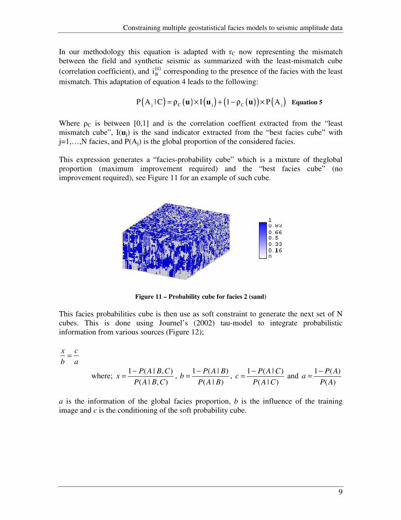
Where �C is between [0,1] and is the correlation coeffient extracted from the “least mismatch cube”, I(uj) is the sand indicator extracted from the “best facies cube” with j=1,…,N facies, and P(Aj) is the global proportion of the considered facies. This expression generates a “facies-probability cube” which is a mixture of theglobal proportion (maximum improvement required) and the “best facies cube” (no improvement required), see Figure 11 for an example of such cube.

Figure 11 – Probability cube for facies 2 (sand) This facies probabilities cube is then use as soft constraint to generate the next set of N cubes. This is done using Journel’s (2002) tau-model to integrate probabilistic information from various sources (Figure 12);

ac

bx =

where; ),|(

),|(1CBAP

CBAPx

−= , )|(

)|(1BAP

BAPb

−= , )|(

)|(1CAP

CAPc

−= and )(

)(1AP

APa

−=

a is the information of the global facies proportion, b is the influence of the training image and c is the conditioning of the soft probability cube.


10

Figure 12 – Next generation of simulations conditioned to the training image, rotation/affinity and probability cubes

This iterative algorithm is run until the global mismatch between the synthetic seismic of the facies model and the field seismic data reach an optimal minimum. In Figure 16 is possible to see a summary of the algorithm. Results To illustrate the method, 6 iterations were computed with N=30 simulations on the Stanford VI dataset. Note that we assume available perfect geological information and a perfect forward model. The algorithm converges as shown by a systematic increase in the global correlation coefficient between model and amplitude data, see Graphic 1. The facies model with the highest correlation out of 30 models in the last iteration has a correlation of 0.88,

N

Simulated Facies

CO-MPS

Training Image

Rotation Affinity

Probability facies 1 Probability facies 2


11

Graphic 1 – Convergence of the algorithm Figure 17 shows the progression of the average of the simulations which shows an increase in certainty (more values close to zero (mud) or one (sand)). The final facies model is shown in Figure 13, and at least visually, does not contain any artifacts, i.e. reproduces well the geological continuity of the training image. To check how well the seismic amplitude data is reproduced we forward simulate the seismic on the best facies model, see Figure 13. Clearly the method matches well the field seismic, particularly when compared with the probabilistic approach

Progress

60.49

24.17

0.17

0.88

0

10

20

30

40

50

60

70

1 2 3 4 5 6

Iterations

Dife

renc

e

0

0.1

0.2

0.3

0.4

0.5

0.6

0.7

0.8

0.9

1

Cor

rela

tion

Best Minimum Diference Best Global Correlation


12

Figure 13 – Comparison between the two methods In Figure 14 some slices of the results are presented, where it is possible to see some similarities between the seismic response of the proposed approach and the reference data seismic amplitude.

Figure 14– Correlation slices For the multi-point simulation we make use of the same training image with rotation and affinity associated as the one with which the reference dataset was created. To test the robustness of the proposed method to lack of knowledge about the spatial model a

Facies Cube Facies Cube

� = 0.88

Facies Cube

� = 0.20

Seismic Amplitude Field Seismic Seismic Amplitude

(Reference Data) (Proposed Approach) (Probabilistic Approach)

Forward Modeling Forward Modeling Forward Modeling

Correlation Correlation

(Reference Data) (Proposed Approach) (Probabilistic Approach)

Seismic Amplitude Seismic Amplitude Seismic Amplitude


13

different training image is used, consisting on the previous training image rotated 90º, and with no rotation and affinity. The same test is re-run. As previously, 6 iterations were computed with 30 simulations. The method still converges, even though the results are not as perfect matching as before: a correlation coefficient with the field seismic of 0.83 (Graphic 2) can be obtained.

Graphic 2 – Convergence of the algorithm with changes in the prior model Although in this facies model the channels are not so independents and identifiable (Figure 15), after applying the low-pass filter the final seismic amplitudes show more similarities to the “real” seismic amplitude. This is due to the fact that different images subject to the same low-pass filter can yield the same result (ill-posed inverse problem).

Progress

62.74

28.99

0.14

0.83

0

10

20

30

40

50

60

70

1 2 3 4 5 6

Iterations

Dife

renc

e

0

0.1

0.2

0.3

0.4

0.5

0.6

0.7

0.8

0.9

Cor

rela

tion

Best Minimum Diference Best Global Correlation


14

Figure 15– Final facies model (left), acoustic impedance (middle) and the forwarded seismic amplitude (right) produced with changes in the prior model

Parameters sensitivity As stated previously, the local minimum depends on the parameters used to calculate the mismatches. In this section some parameters sensitivity is further analysed. Number of iterations In the first iteration the main optimization is obtained, after this the process tends to stabilize (Graphic 3). Hence, without changing any of the other parameters, the number of iterations does not have a big influence on the optimization. Number of facies simulations N per iterations This parameter can have a major influence on the optimization: with numerous simulations the process has a wide variety of possibilities to choose from, and can build a more precise best-facies cube, but if the simulations are very alike, the choice of N will not matter.

Graphic 3 – Influence of different number of iterations (1 to 6) and simulations (20, 30 and 40).


15

Graphic 3 compares the values of correlation and average difference of the simulation model with the best result for different number of facies models N simulated. These values are presented only for the first and last iterations. For the first iteration the difference is not very noticeable, but in the last iteration the correlation value is higher as the number of simulations increases. Criterion of convergence The criterion of differences is more precise than the correlation, since the correlation gives us a value of the similarity between two sets of data, while the difference is more susceptible to different patterns or small variation in the patterns. But to calculate the probabilities the correlations are needed. Size of the columns In the previous test the cubes were divide in 4 layers with 20 values each column. Since the correlation has some sensitivity to the number of data used, the results also change. For a largest column the convergence will tend to be slower, since it is more difficult to match an entire column than piece-wise matching. In general we recommend that the number of layers chosen depends on the vertical resolution of the seismic data, i.e. for lower resolution less layer could be retained. References Bortoli, L.J. (1992) Selection of stochastic reservoir models using iterative forward matching of seismic traces, SCRF 1992. Castro, S., Caers, J and Mukerji Y, “The Stanford VI reservoir”, SCRF 2005. Goovaerts, P., 1977, Geostatistics for Natural Resources Characterization (New York: Oxford University Press) Caers, J., 2003. History matching under training-image based geological model constraints. SPE Journal, v. 7: 218-226. Journel, A.G., “Combining knowledge form diverse information sources: an alternative to Bayesian analysis”. Mathematical Geology, V. 34, No. 5, 573-598, 2002. Strebelle, S.: “Conditioning Simulation of Complex Structures Multiple-Point Statistics”, Mathematical Geology, v. 34, No. 1, January 2002.


16

Figure 16 – Summary of the algorithm

SNESIM

Wavelet

COSNESIM

Iterations until an optimal global

correlation

N simulations

N simulations

Populate the facies

Forward Modeling

Mismatch

Build Probability

Model

Mismatch Cubes

Training Image Facies Cube Impedance Cube Amplitude Cube “Real” Amplitude

Training Image

Probability Models

Best Facies Cube

Best Mismatch Cube

Filter


17

Figure 17 – Average of the 30 simulations for each iteration

Iter. 1 Iter. 2 Iter. 3

Iter. 4 Iter. 5 Iter. 6

sand

mud

constraining multiple-point facies models to seismic...

Documents