Spatiotemporal Pattern Mining for NowcastingExtreme Earthquakes in Southern California

Bo FengIntelligent Systems EngineeringIndiana University Bloomington

Bloomington, Indiana, USAEmail: fengbo@iu.edu

Geoffrey C. FoxIntelligent Systems EngineeringIndiana University Bloomington

Bloomington, Indiana, USAEmail: gcf@indiana.edu

Abstract—Geoscience and seismology have utilized the mostadvanced technologies and equipment to monitor seismic eventsglobally from the past few decades. With the enormous amount ofdata, modern GPU-powered deep learning presents a promisingapproach to analyze data and discover patterns. In recentyears, there are plenty of successful deep learning models forpicking seismic waves. However, forecasting extreme earthquakes,which can cause disasters, is still an underdeveloped topic inhistory. Relevant research in spatiotemporal dynamics miningand forecasting has revealed some successful predictions, a crucialtopic in many scientific research fields. Most studies of them havemany successful applications of using deep neural networks. InGeology and Earth science studies, earthquake prediction is oneof the world’s most challenging problems, about which cutting-edge deep learning technologies may help discover some valuablepatterns. In this project, we propose a deep learning modelingapproach, namely EQPRED, to mine spatiotemporal patternsfrom data to nowcast extreme earthquakes by discovering visualdynamics in regional coarse-grained spatial grids over time. Inthis modeling approach, we use synthetic deep learning neuralnetworks with domain knowledge in geoscience and seismologyto exploit earthquake patterns for prediction using convolutionallong short-term memory neural networks. Our experiments showa strong correlation between location prediction and magnitudeprediction for earthquakes in Southern California. Ablationstudies and visualization validate the effectiveness of the proposedmodeling method.

Index Terms—Spatiotemporal, Convolution, Recurrent NeuralNetwork, LSTM, Temporal Convolution, Nowcasting

I. INTRODUCTION

Spatial and temporal attributes have played an essential rolein addressing scientific issues mathematically and statisticallywith large volumes of data in real problems. A worldwide teamof scientists studied the published datasets from The WorldPopproject (www.worldpop.org) for discovering the spatiotemporalpattern of population in China from 1990 to 2010 [1]. Formodern Geoscience, spatiotemporal modeling has been studiedfor a long time. In this book [2], authors summarized someinitial efforts by utilizing spatiotemporal features for scientificinterpretation and prediction.

Tradition machine learning algorithms like the support vectormachine (SVM) and decision trees perform well on smalldatasets. Optimization methods such as stochastic gradientdescent (SGD) enable the deep learning algorithms can betrained in small batches for extensive data without sacrificing

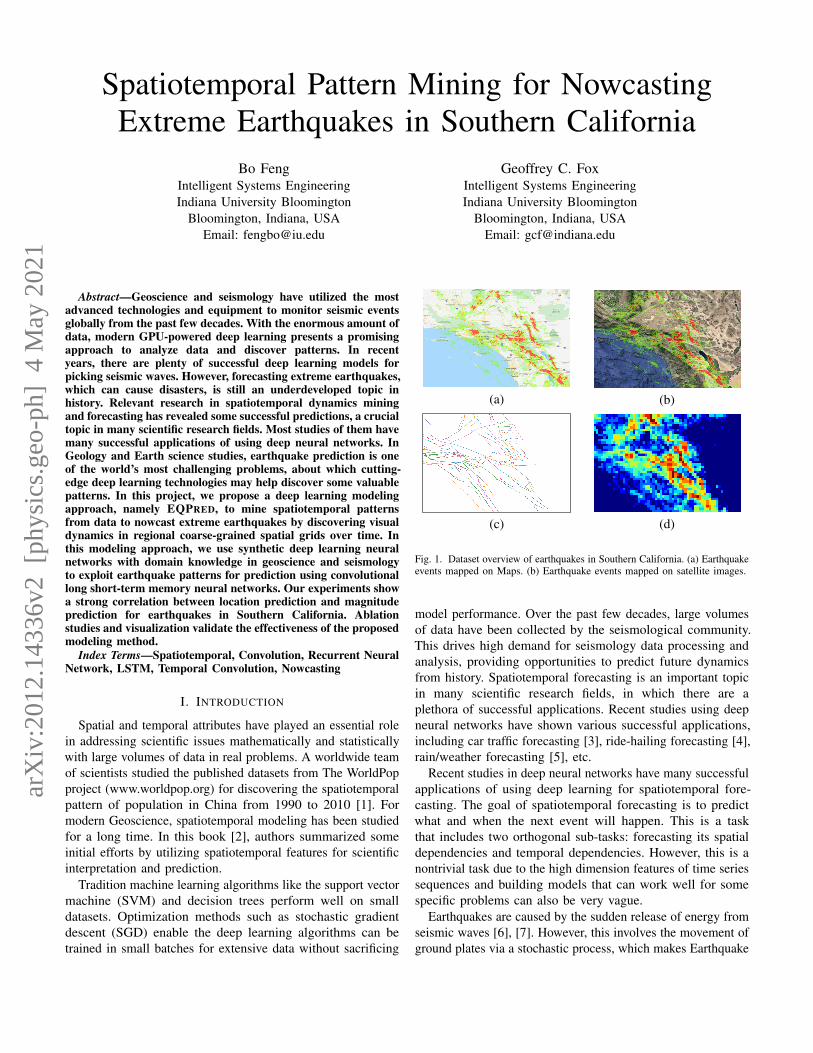
(a)

(c)

(b)

(d)

Fig. 1. Dataset overview of earthquakes in Southern California. (a) Earthquakeevents mapped on Maps. (b) Earthquake events mapped on satellite images.

model performance. Over the past few decades, large volumesof data have been collected by the seismological community.This drives high demand for seismology data processing andanalysis, providing opportunities to predict future dynamicsfrom history. Spatiotemporal forecasting is an important topicin many scientific research fields, in which there are aplethora of successful applications. Recent studies using deepneural networks have shown various successful applications,including car traffic forecasting [3], ride-hailing forecasting [4],rain/weather forecasting [5], etc.

Recent studies in deep neural networks have many successfulapplications of using deep learning for spatiotemporal fore-casting. The goal of spatiotemporal forecasting is to predictwhat and when the next event will happen. This is a taskthat includes two orthogonal sub-tasks: forecasting its spatialdependencies and temporal dependencies. However, this is anontrivial task due to the high dimension features of time seriessequences and building models that can work well for somespecific problems can also be very vague.

Earthquakes are caused by the sudden release of energy fromseismic waves [6], [7]. However, this involves the movement ofground plates via a stochastic process, which makes Earthquake

arX

iv:2

012.

1433

6v2

[ph

ysic

s.ge

o-ph

] 4

May

202

1

forecasting is a worldwide challenging problem. Scientistsaround the world have built an enormous number of detectorsfor picking up earthquake signals. It is a general belief thatearthquakes are predictable under some assumption that quakesare formed underneath the Earth are accumulated stresses ina gradual process over a long time. In this case, it would bepossible to predict earthquake shocks for future activities ofquakes by learning patterns from historical seismic events.

Conventionally, earthquakes are located through a processof detecting signals, picking up arrival time, and estimatingepicenters of events using a velocity model. Efforts have beenmade to filter P-waves and S-waves from the original waveformsignals of earthquakes and seismic noise [7]. In this project,our goal is to utilize the preprocessed seismic signals formingepicenters (location labels) to forecast the probabilities of thesubsequent earthquakes in an area.

Earthquake forecasting consists of three major tasks inmachine learning. The first task is to predict when the nextseismic event will happen in a specific region. The secondtask is to predict whether or not the next seismic event willcome. The third task is to predict the level of magnitude ofthe upcoming seismic events to predict major shocks.

Deep learning neural networks have presented a widelysuccessful approach to capture spatial-temporal dependencies ofproblems to achieve accurate forecasting results. Convolutionalneural networks have achieved convinced success in computervision, image object recognition, etc [8]. Here we test thehypothesis that earthquake patterns can be perceived by learninghistorical seismic events. However, epicenters’ prediction islearned from annotated seismograms. Due to the uncertaintiesof earthquakes, even the ground truth labels that are annotatedby domain experts may be biased. Locations and magnitude ofepicenters are maybe adjusted after the seismic event happeneda long while.

In this project, we propose joint modeling of using a selfsupervised autoencoder (AE) and temporal convolutional neuralnetworks (TCN) [9] for earthquake prediction by modelingspatiotemporal dependencies in Southern California. Addition-ally, EQPRED comprehensively improves the autoencoder andTCN by incorporating skip connections and local temporalattention mechanisms. Compared to conventional recurrentneural networks or a single model, our joint modeling presentssome advantages in predicting major shocks in the area ofstudy. In summary:• We study the earthquake dataset for Southern California

and reconstruct the time series events into a sequence of2D images.

• We model the spatiotemporal dependencies of earthquakesin Southern California with an improved autoencoder andTCN neural networks and show some preliminary butpromising results for nowcasting events in contrast to 11baseline models.

This paper is organized as following: Section II reviewsrelated work in four aspects. In Section III, we propose aspatiotemporal modeling approach, namely EQPRED, andillustrate the how spatial and temporal dynamics are modeled

theoretically. In Section IV, we show the detailed implemen-tation of EQPRED, run analysis on the dataset, and evaluatethe effectiveness. Finally, we conclude in Section V with thediscussion of the limitations and future research directions.

II. RELATED WORK

Four subjects are related to this project: 1) predictingepicenters only with advanced machine learning techniques;2) spatiotemporal modeling in a broad range of applications;3) advanced dynamic pattern mining and prediction in visualapplications; 4) extreme event prediction in other areas ofresearch.

A. Convolutional Methods in Predicting Epicenters

Estimating and predicting the epicenters of earthquakeshas a long history. Scientists from Geophysics, Geology,and Seismology have developed various tools and analyticalfunctions to predict epicenters from datasets. In 1997, Bakunand Wentworth suggested using Modified Mercalli intensitydatasets for Southern California earthquakes to bound theepicenter regions and magnitudes [6]. In 1998, Pulinetsproposed predicting epicenters of strong earthquakes with thehelp of satellite-sounding systems. Scientists from Greece hadillustrated a successful project which predicted the prominentaspects of earthquakes using seismic electric signals [10].Recently, Guangmeng et al. attempted to predict earthquakeswith satellite cloud images and revealed some possibilities ofpredicting earthquakes using geophysics data [11]. Zakaria etal. presented their work of predicting epicenters by monitoringprecursors, such as crustal deformation anomalies and thermalanomalies, with remote sensing techniques [12]. These studieseither used only too little data or too simple analytical models.

B. Spatiotemporal Dynamics and Generative Models

Most recently, it is a prevailing method to make predictionsby modeling the spatiotemporal dynamics for domain scienceproblems. This is because large volumes of data are increasinglycollected in the vast majority of domains including, socialscience, epidemiology, transportation, and geoscience. Cui etal. proposed to use graph convolutional long short-term memoryneural networks to predict traffic via capturing spatial dynamicsfrom the car traffic patterns [13]. Li et al. utilized a seq2seqneural network architecture to capture spatial and temporaldependencies for traffic forecasting by incorporating a diffusionfilter in convolutional recurrent layers [3]. FUNNEL was aproject proposed by Matsubara [14]. It was designed to usean analytical model and a fitting algorithm for discoveringspatial-temporal patterns of epidemiological data.

C. Visual Pattern Prediction

Lotter et al. presented a model to predict video frames withdeep predictive coding networks [15], which was based on theConvLSTM2D network module with specific top-down statesupdating algorithm. [16] is another example in predicting videoframes. The authors of this work presented the effectivenessof modeling object motion via predicting future object pixels.

2

For example, a ball moves and a block falls. These models aresuccessful for predicting contiguous and dense image frames,whereases the earthquake data are very sparse, the extremeshocks are very rare in terms of probability.

D. Extreme rare event prediction

Laptev et al. [17] proposed their modeling to predict rare tripdemands for ride-hailing service. In that paper, they built an end-to-end architecture using joint modeling by combining LSTMautoencoder and LSTM predictor networks. They showed theirforecasting capability on a Uber’s public dataset. Geng etal. [18] proposed another model to forecast the ride-hailingdemand using graph-based recurrent neural networks, in whichgraphs are defined by road networks with Euclidean and non-Euclidean distances. We compared this approach with ourEQPRED, a detailed discussion of which is in Section IV-C.

III. EQPRED MODELING

Earthquakes come with an epicenter which is a point atthe surface on Earth, and the mainshocks of quakes areregarded as the main contribution to significant disasters. Tomodel the spatiotemporal patterns of earthquake shocks, wefirstly consider the data attributes of specialty, which arediscussed in Subsection III-A, then we pre-process the data inSubsection III-B, and then the spatial and temporal dynamicsare modeled in Subsection III-C, III-D respectively.

The proposed prediction model consists of two majorcomponents, an autoencoder which learns the latent spacedistribution from the image-like view of the earthquakes, anda prediction network that learns to predict the likelihood ofthe next main shock happening within the same area.

A. Energy-based Data Models

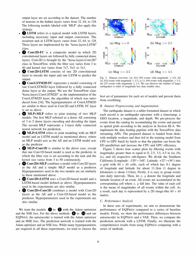
Geographical data are coordinates related. Intuitively, thoseshocks that happened in different Geo terrain may take effectto future shocks unevenly. The earthquake dataset used in thisproject is a tablet formatted catalog containing information onshocks in terms of geo-coordinates and magnitudes. In thisproject, we focus on the time and geolocation of shocks, otherattributes like types of quakes are not included. This datasetcovers all earthquake events in Southern California from theyear 1990 to 2019. The full dataset is used in all the followingexperiments. Figure 1 shows all events plotted in 2D maps,in which hot spots are areas where earthquakes frequentlyhappened or big earthquakes happened in history. Figure 3shows scatter plots of events with magnitudes equal and greaterthan 0, 2.5, 3.5, 4.5, respectively, where extreme cases are order-of-magnitude large quakes pre-defined by a picked thresholdin this project according to the domain knowledge.

Seismometers record seismic events by calibrating thevibrations of waves. Magnitude in the dataset representsmeasured amplitude as a measured seismogram. While theyare discrete data points, accumulating magnitudes by summingthem up by averaging makes the temporal information lossand deemphasizes large earthquakes. In contrast to magnitude,earthquakes release energy can help mitigate this issue by two

folds: 1) accumulated energy value in a region can representthe energy released by the stress of Earth over time; 2) energydata model naturally highlights large events since the energy oflarge events can be an order of magnitude higher than that ofsmall events. The formula of converting earthquake magnitudeto energy defines as:

E = (10Mag)3/2 (1)

in which the magnitude 0 ≤ Mag ∈ R ≤ 10. Earthquakemagnitude value can be even negative for tiny events thatare negligible. This scale is also open-ended, but events withmagnitude values greater than 10 are clipped to 10.

B. Location-aware Data Weaving

As a time-series prediction task, the earthquake catalogcontains locations and magnitudes, which could be usedas target properties. However, it could be more natural toreorganize the vector-valued 1D time-series dataset into a2D sequence dataset by dividing a map region into smallboxes according to longitudes and latitudes and aggregating thereleased energy within a small box per specific time-frequency.

Long short-term memory (LSTM) [19] is an advanced modelof recurrent neural networks suitable for modeling series-like vector-valued data. Compared with the exiting LSTMapproach such as [20], location-aware weaving gives finer-grained geolocations. Besides, 2D convolutional operationscan put a strong prior on locations than the recurrent matrixmultiplication for vector-valued observations in LSTM cells.Furthermore, for earthquakes, the underlying intuition is that2D convolution may capture location-based plate movements,which is considered as the direct cause of earthquakes.

We denote Magtk the value at location k and time t of a

spatially and temporally continuous phenomenon of interest.So each element of the sequence becomes a summation ofall energy released at the grid (i, j), given i ∈ [0,M) andj ∈ [0, N). Then the total energy for each grid element isdefined in Eq 2 , which means Xt has a shape M ×N for Mboxes along the latitude and N boxes along the longitude.

Xti,j =

∑k∈grid[i][j]

((10Magtk)3/2) (2)

Considering this area as a 2D mesh grid, this equation sumsup all energy erupted in every grid for each time interval. Forexample, we can sum up how much energy released within abox region of Longitude from -120 to -119 and Latitude from32 to 33 everyday.

C. Convolutional AutoEncoder for Effective Spatial Modeling

Main shocks with large magnitudes are rare in terms ofstatistics and nature physics. In addition, earthquakes are fullof stochastic processing, resulting in seismic signals are verynoisy. To predict the future mainshocks, we first model thespatial patterns within the southern California area.

We use an autoencoder to mine the spatial pattern changesunder normal circumstances and abnormal circumstances. Asshown in Figure 2, the autoencoder consists of three major

3

Encoder:mlayers Decoder:nlayers

Dilatedcausalconvolutionlayers

Connection1

Connection2

60x4060x4060x40... 60x4060x4060x40 ...

Prediction

Normalimages

AutoEncoderNetworks

PredictionNetworksX0,...,XT X0,...,XT

Reconstructedimages

L

yt+1

Localtemporalattention

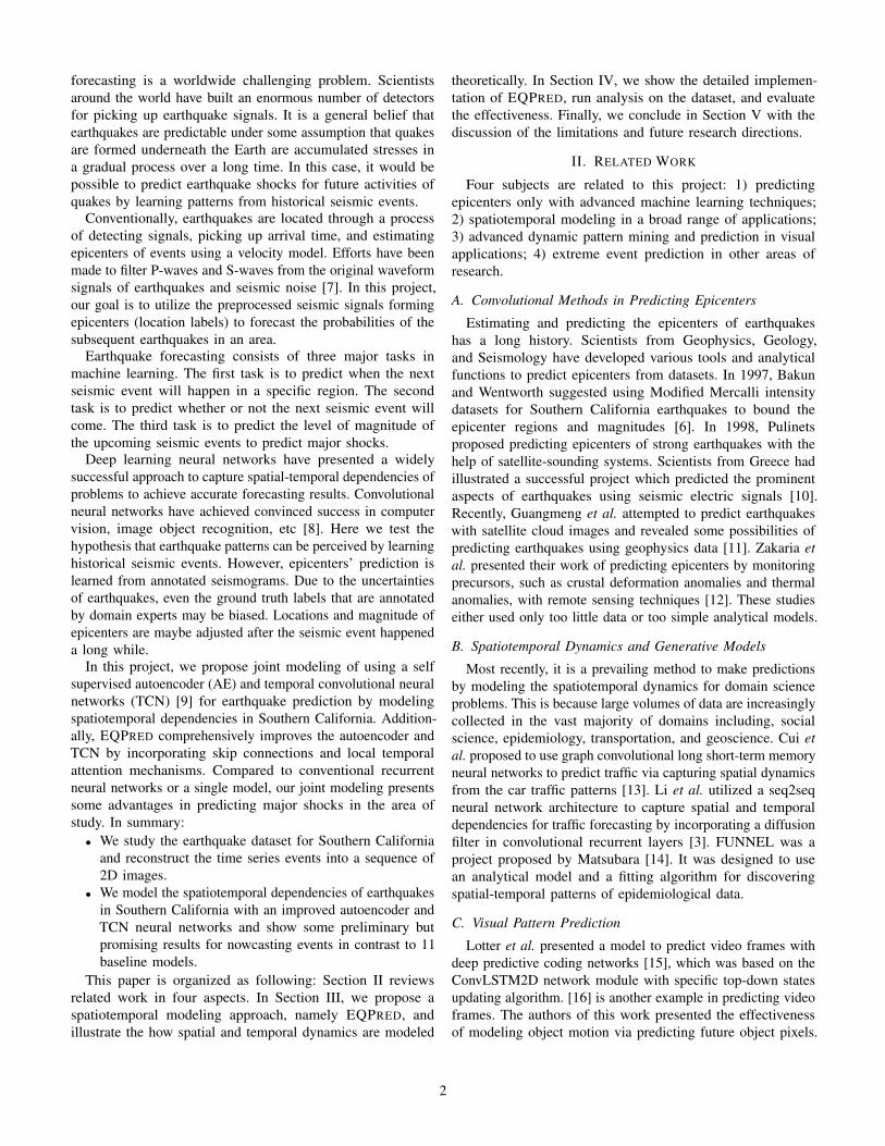
Fig. 2. EQPRED: overview of earthquake prediction networks.

components: 1) a bunch of convolutional layers encodes theinput to 2) the bottleneck layer in green color, and 3) the layersin decoder up-sample the latent variables from the bottlenecklayer to the output. Compared to the variational autoencoder(VAE), we do not assume Gaussian distribution or any otherdistributions for the latent space. In addition, the reconstructedresults from VAE are tended to be noisier. We also make someexperiments for complete comparison in Section IV. Spatialmodeling is a semi-supervised process to train a model thatlearns the representation of earthquake images. We train thismodel by minimizing the following equation.

L(Xnormal, g(f(Xnormal)) + Ω(h,Xnormal) (3)

, where Xnormal are images of earthquakes with magnitudesless than a threshold, f is an encoder function, g is an decoderfunction, and Ω is a function that regularizes or penalizes thecost. This setup enforces the same input and output so that thebottleneck layer can obtain the most critical latent variablesfrom the dataset. Detailed modeling methods used in AE arecovered in the following sub-sections.

1) Spatial modeling: The encoder networks are comprised ofconvolutional layers followed by Batch Normalization with theReLU activation function. The decoder networks are comprisedof de-convolutional layers with the ReLU activation function.After the seismic events are parsed and transformed to 2Dimage-like sequences in Section III-A, we can utilize the spatialdependencies between pixels. Convolutional operations arecommon image feature extraction means. Pixel relationshipscan be easily mapped to geology locations of events. Theencoder component of this model is used to extract the spatialfeatures from images which contribute to convolution layers in adownsampling manner. The downsampled feature maps enablethe network to collect contextual information, which could besurface terrains on Earth. In convolution-base layers with akernel K, the process takes the input X with the followingform:

Si,j =∑m

∑n

X(i+m, j + n)K(m,n) (4)

The decoder component of this model is used for upsamplingvariables from the bottleneck layer by inverse 2D convolutionaloperations. The final reconstructed image denoted as X isproduced by the decoder.

2) Skip connections: We incorporate skip connections inthe AutoEncoder architecture. Skip connections are forwardshortcuts between layers in networks. Skip connections can helprecover the full spatial resolution at the network output to avoidthe gradient vanishing, making fully convolutional methodssuitable for modeling segments on maps. They symmetricallyconnect layers from the encoder and decoder, as shown inFigure 2. This strategy allows long skip connections to passfeatures from the encoder path to the decoder path directly,which can recover spatial information lost due to downsampling,according to [21]. The combination of low-level features andhigh-level features improves the training performance due tolarge gradients and improves accuracy due to complementaryinformation summarized from different levels. Both long andshort connections are used in the model as shown “Connection1” and “Connection 2” in Figure 2.

The AE includes the bottleneck layer and other basicblocks. The design benefits of those are introduced in [22],[21]. For instance [23] includes short skip connections fordetecting salient objects. Skipping some blocks with minimalmodification encourages the information to pass through thenon-linear functions to learn a residual representation from thedirect input information. Similar to the short skip connections inResidual Networks [24], we sum the features from the encoderlayers on the expanding path of decoder layers with long skipconnections symmetrically.

3) Bottleneck layer: Hidden latent variables captured in thebottleneck layer have shown effectiveness in many applications,e.g. [3], [25]. The bottleneck layer in the autoencoder isdeliberately set to a small vector of a size k feature map.This layer creates restrictions in the network to enforce theinformation pertaining to low dimensional space. Firstly, itregularizes the model from overfitting all samples. Secondly, asmall feature map can better differentiate abnormal cases fromnormal cases. We set this k as a hyperparameter in our model.

4

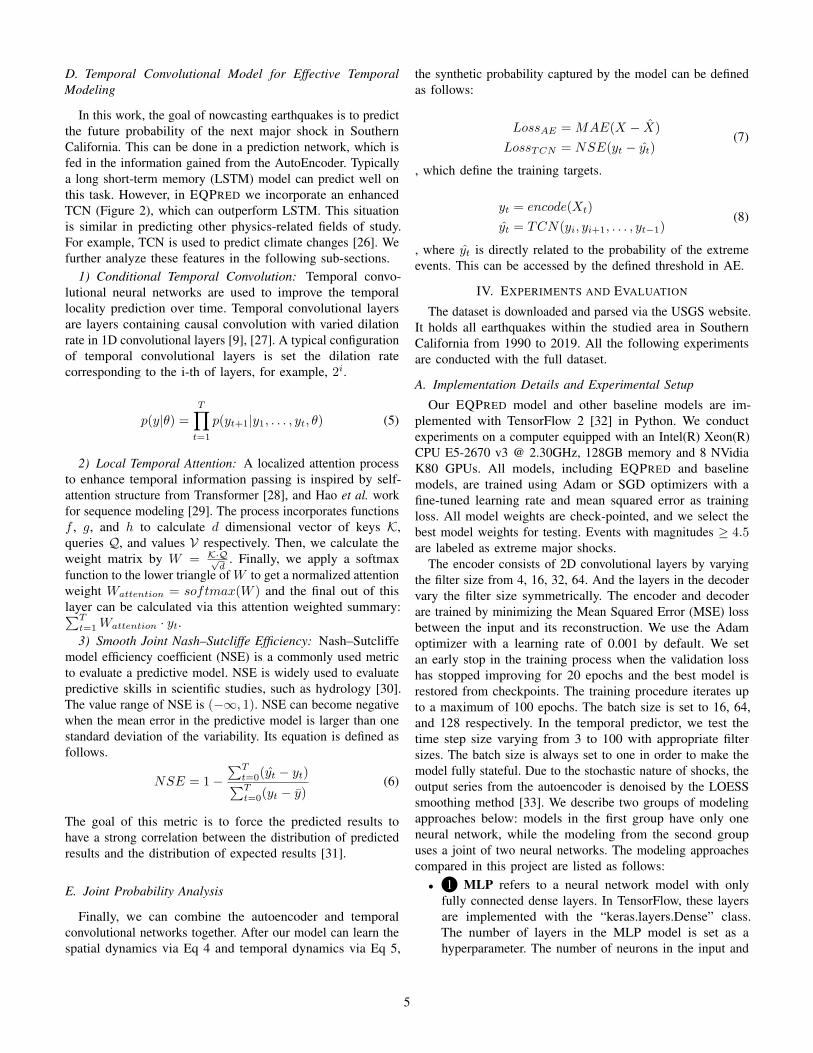
D. Temporal Convolutional Model for Effective TemporalModeling

In this work, the goal of nowcasting earthquakes is to predictthe future probability of the next major shock in SouthernCalifornia. This can be done in a prediction network, which isfed in the information gained from the AutoEncoder. Typicallya long short-term memory (LSTM) model can predict well onthis task. However, in EQPRED we incorporate an enhancedTCN (Figure 2), which can outperform LSTM. This situationis similar in predicting other physics-related fields of study.For example, TCN is used to predict climate changes [26]. Wefurther analyze these features in the following sub-sections.

1) Conditional Temporal Convolution: Temporal convo-lutional neural networks are used to improve the temporallocality prediction over time. Temporal convolutional layersare layers containing causal convolution with varied dilationrate in 1D convolutional layers [9], [27]. A typical configurationof temporal convolutional layers is set the dilation ratecorresponding to the i-th of layers, for example, 2i.

p(y|θ) =

T∏t=1

p(yt+1|y1, . . . , yt, θ) (5)

2) Local Temporal Attention: A localized attention processto enhance temporal information passing is inspired by self-attention structure from Transformer [28], and Hao et al. workfor sequence modeling [29]. The process incorporates functionsf , g, and h to calculate d dimensional vector of keys K,queries Q, and values V respectively. Then, we calculate theweight matrix by W = K·Q√

d. Finally, we apply a softmax

function to the lower triangle of W to get a normalized attentionweight Wattention = softmax(W ) and the final out of thislayer can be calculated via this attention weighted summary:∑T

t=1Wattention · yt.3) Smooth Joint Nash–Sutcliffe Efficiency: Nash–Sutcliffe

model efficiency coefficient (NSE) is a commonly used metricto evaluate a predictive model. NSE is widely used to evaluatepredictive skills in scientific studies, such as hydrology [30].The value range of NSE is (−∞, 1). NSE can become negativewhen the mean error in the predictive model is larger than onestandard deviation of the variability. Its equation is defined asfollows.

NSE = 1−∑T

t=0(yt − yt)∑Tt=0(yt − y)

(6)

The goal of this metric is to force the predicted results tohave a strong correlation between the distribution of predictedresults and the distribution of expected results [31].

E. Joint Probability Analysis

Finally, we can combine the autoencoder and temporalconvolutional networks together. After our model can learn thespatial dynamics via Eq 4 and temporal dynamics via Eq 5,

the synthetic probability captured by the model can be definedas follows:

LossAE = MAE(X − X)

LossTCN = NSE(yt − yt)(7)

, which define the training targets.

yt = encode(Xt)

yt = TCN(yi, yi+1, . . . , yt−1)(8)

, where yt is directly related to the probability of the extremeevents. This can be accessed by the defined threshold in AE.

IV. EXPERIMENTS AND EVALUATION

The dataset is downloaded and parsed via the USGS website.It holds all earthquakes within the studied area in SouthernCalifornia from 1990 to 2019. All the following experimentsare conducted with the full dataset.

A. Implementation Details and Experimental Setup

Our EQPRED model and other baseline models are im-plemented with TensorFlow 2 [32] in Python. We conductexperiments on a computer equipped with an Intel(R) Xeon(R)CPU E5-2670 v3 @ 2.30GHz, 128GB memory and 8 NVidiaK80 GPUs. All models, including EQPRED and baselinemodels, are trained using Adam or SGD optimizers with afine-tuned learning rate and mean squared error as trainingloss. All model weights are check-pointed, and we select thebest model weights for testing. Events with magnitudes ≥ 4.5are labeled as extreme major shocks.

The encoder consists of 2D convolutional layers by varyingthe filter size from 4, 16, 32, 64. And the layers in the decodervary the filter size symmetrically. The encoder and decoderare trained by minimizing the Mean Squared Error (MSE) lossbetween the input and its reconstruction. We use the Adamoptimizer with a learning rate of 0.001 by default. We setan early stop in the training process when the validation losshas stopped improving for 20 epochs and the best model isrestored from checkpoints. The training procedure iterates upto a maximum of 100 epochs. The batch size is set to 16, 64,and 128 respectively. In the temporal predictor, we test thetime step size varying from 3 to 100 with appropriate filtersizes. The batch size is always set to one in order to make themodel fully stateful. Due to the stochastic nature of shocks, theoutput series from the autoencoder is denoised by the LOESSsmoothing method [33]. We describe two groups of modelingapproaches below: models in the first group have only oneneural network, while the modeling from the second groupuses a joint of two neural networks. The modeling approachescompared in this project are listed as follows:• 1 MLP refers to a neural network model with only

fully connected dense layers. In TensorFlow, these layersare implemented with the “keras.layers.Dense” class.The number of layers in the MLP model is set as ahyperparameter. The number of neurons in the input and

5

output layer are set according to the dataset. The numberof neurons in the hidden layers varies from 32, 64, to 128.The following models labeled with ‘MLP’ also apply thisstrategy.

• 2 LSTM refers to a typical model with LSTM layers,including necessary input and output conversion. Therecurrent unit in LSTM layers varies from 32, 64, to 128.These layers are implemented by the “keras.layers.LSTM”class.

• 3 Conv2D-FC is a composite model in which 2Dconvolutional layers are followed by fully connected denselayers. Conv2D is brought by the “keras.layers.Conv2D”class in TensorFlow, while the filter size varies from 3 to40 and kernel size varies from 7x7, 5x5, to 3x3.

• 4 Conv2D-LSTM consists of one 2D convolutionallayer to encode the input and one LSTM to predict theoutput.

• 5 ConvLSTM2D-FC represents a model consisting ofone ConvLSTM2D layer followed by a fully connecteddense layer as the output. We use the TensorFlow class“keras.layers.ConvLSTM2D” as the implementation of theConvLSTM2D layer, the algorithm of which was intro-duced from [34]. The hyperparameters of ConvLSTM2Dare similar to those used in Conv2D and LSTM. FC layeris set as above.

• 6 MLP+MLP refers to joint training of two MLPmodels. The first MLP refereed as a dense AE consistingof 3 to 5 dense layers encoding and decoding the input.The second MLP represents a 3-layer fully connectedneural network for prediction.

• 7 MLP+LSTM refers to joint modeling with an MLPmodel and an LSTM model as mentioned above, wherean MLP model acts as the AE and an LSTM model actsas the predictor.

• 8 MLP+Conv1D is similar to the above case, exceptthat one Conv1D-based model is used as the predictor, inwhich the filter size is set according to the task and thekernel size varies from 3 to 50 continuously.

• 9 Conv2D+MLP combines a model with Conv2D layersas the AE and a simple MLP model as a predictor.Hyperparameters used in the two models are set similarlyto those mentioned above.

• 10 Conv2D+LSTM uses a Conv2D-based model and aLSTM-based model defined as above. Hyperparametersused in the experiments are also similar.

• 11 Conv2D+Conv1D combines a model with Conv2Dlayers as the AE and a Conv1D-based model as thepredictor. Hyperparameters used in the experiments arealso similar.

We train the models 1 to 5 with the Adam optimizerand the NSE loss. For the above methods 6 to 11 and ourEQPRED, the autoencoder is trained with the Adam optimizerand an MSE loss. The prediction network is trained with theAdam optimizer and an NSE loss. While many hyperparametersare required in all these experiments, we tend to choose the

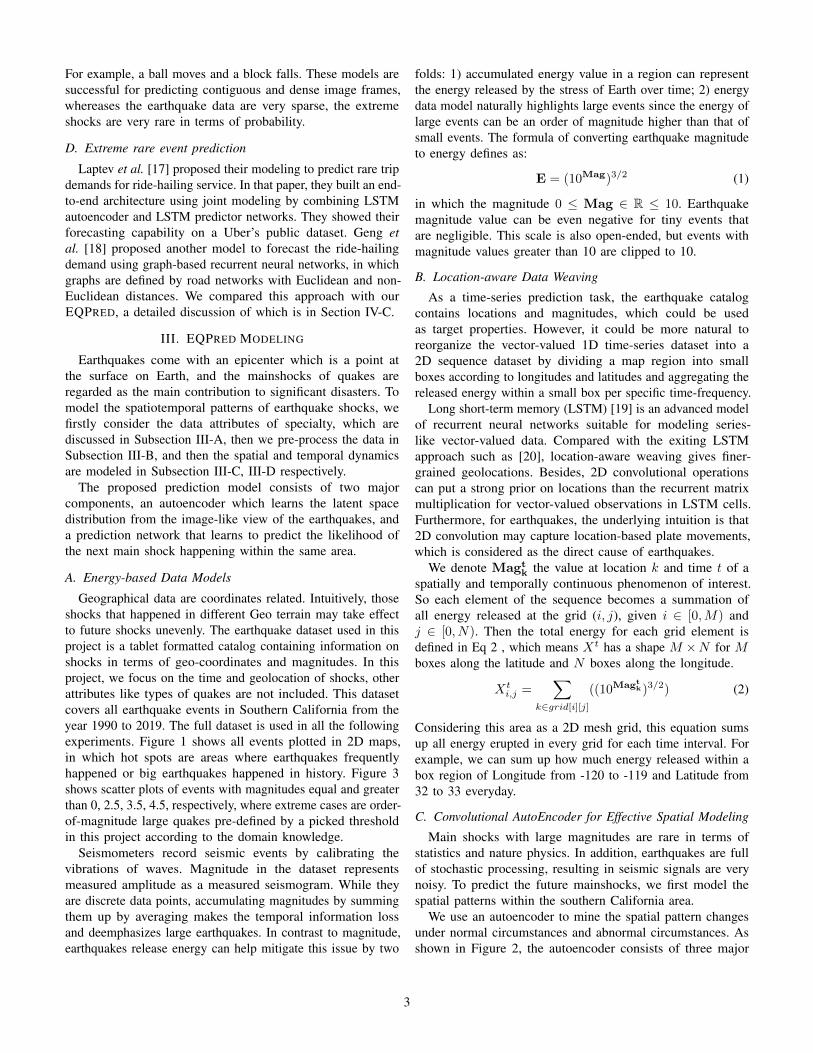
(a) Mag >= 0 (b) Mag >= 2.5

(c) Mag >= 3.5 (d) Mag >= 4.5

Fig. 3. Dataset overview: (a) 444, 589 events with magnitude ≥ 0.0, (b)24, 822 events with magnitude ≥ 2.5, (c) 2, 489 events with magnitude ≥ 3.5,(d) 237 events with magnitude ≥ 4.5. We can observer the number of largerearthquakes is order of magnitude less than smaller ones.

best set of parameters for each set of models and prevent themfrom overfitting.

B. Dataset Preprocessing and Augmentation

The earthquake dataset is a tablet formatted dataset in whicheach record is an earthquake epicenter with a timestamp, aGEO location, a magnitude, and depth. We pre-process theevents from the catalog by accumulating the events and parsedas spatial grids according to the analysis in Section III-A. Weimplement the data feeding pipeline with the TensorFlow datastreaming APIs. The prepared dataset is loaded from diskswith multiple workers and then fed in the training model fromCPU to GPU batch by batch so that the pipeline can boost theI/O parallelism and increase the CPU and GPU efficiency.

Figure 3 shows four scatter plots by filtering events withmagnitudes greater than or equal to 0, 2.5, 3.5, 4.5 in (a), (b),(c), and (d) respective sub-figures. We divide the SouthernCalifornia (Longitude: -120°~-140°, Latitude: +32°~+36°) intoa grid with 60 × 40 cells, each of which has 0.1 degreeof longitude and latitude for about 11.1km (1 degree inkilometers is about 111km). Firstly, it is easy to group eventsinto daily intervals. Then, let x, y denote the longitude andlatitude location of an event. All events are accumulated in thecorresponding cell where x, y fall into. The value of each cellis the mean of magnitudes of all events within the cell. Asa result, each day is represented by a 2D image-like 60× 40matrix.

C. Performance Analysis

In these sets of experiments, we aim to demonstrate theperformance of EQPRED compared to a series of baselinemodels. Firstly, we show the performance differences betweenautoencoder in EQPRED and a VAE. Then, we compare theprediction network with a LSTM. Finally, we illustrate thecomprehensive results from using EQPRED comparing with aseries of methods.

6

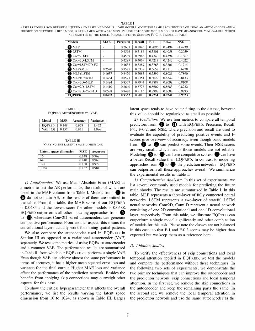
TABLE IRESULTS COMPARISON BETWEEN EQPRED AND BASELINE MODELS. SOME MODELS ADOPT THE SAME ARCHITECTURE OF USING AN AUTOENCODER AND APREDICTION NETWORK. THESE MODELS ARE NAMED WITH A ‘+’ SIGN. PLEASE NOTE SOME MODELS DO NOT HAVE MEANINGFUL MAE VALUES, WHICH

ARE OMITTED IN THE TABLE. PLEASE REFER TO SECTION IV-C FOR MORE DETAILS.

Models MAE Precision Recall F-1 F-0.2 NSE1 MLP - 0.2631 0.2845 0.2096 0.2494 -1.47392 LSTM - 0.4596 0.5186 0.3801 0.4058 -0.20593 Conv2D-FC - 0.4589 0.3963 0.4340 0.4394 -0.18674 Conv2D-LSTM - 0.4299 0.4069 0.4217 0.4243 -0.40225 ConvLSTM2D-FC - 0.4633 0.3289 0.3763 0.3801 -0.17146 MLP+MLP 0.2570 0.7525 0.6338 0.6652 0.7113 0.67787 MLP+LSTM 0.1637 0.8420 0.7085 0.7599 0.8021 0.78908 MLP+Conv1D 0.1484 0.8571 0.9351 0.8029 0.8342 0.81339 Conv2D+MLP 0.1484 0.8577 0.7944 0.7887 0.8098 0.810810 Conv2D+LSTM 0.1410 0.8640 0.8776 0.8609 0.8683 0.822211 Conv2D+Conv1D 0.0588 0.9420 0.9115 0.8998 0.8688 0.9293EQPRED 0.0483 0.9563 0.9016 0.9251 0.9341 0.9323

TABLE IIEQPRED AUTOENCODER VS. VAE.

Model MSE Accuracy VarianceEQPRED 0.148 0.968 1.432VAE [35] 0.157 0.971 1.986

TABLE IIIVARYING THE LATENT SPACE DIMENSION.

Latent space dimension MSE Accuracy16 0.148 0.96864 0.140 0.968128 0.138 0.9721024 0.137 0.984

1) AutoEncoder: We use Mean Absolute Error (MAE) asa metric to test the AE performance, the results of which arelisted in the MAE column from Table I. Models from 1 to6 do not contain AE, so the results of them are omitted in

the table. From this table, the MAE score of our EQPREDis 0.0483 and the lowest score for other models is 0.0588.EQPRED outperforms all other modeling approaches from 6to 11, whereases Conv2D-based autoencoders can generatecompetitive performance. From another aspect, this means theconvolutional layers actually work for mining spatial patterns.

We also compare the autoencoder used in EQPRED inSection III as opposed to a variational autoencoder (VAE)separately. We test some metrics of using EQPRED autoencoderand a common VAE. The performance results are summarizedin Table II, from which our EQPRED outperforms a single VAE.Even though VAE can achieve almost the same performance interms of accuracy, it has a higher mean squared error loss andvariance for the final output. Higher MAE loss and varianceaffect the performance of the prediction network. Besides thebenefits from applying skip connections may outweigh otheraspects for this case.

To show the critical hyperparameter that affects the overallperformance, we list the results varying the latent spacedimension from 16 to 1024, as shown in Table III. Larger

latent space tends to have better fitting to the dataset, howeverthis value should be regularized as small as possible.

2) Prediction: We use four metrics to compare all temporalpredictors from 1 to 11 with EQPRED: Precision, Recall,F-1, F-0.2, and NSE, where precision and recall are used toevaluate the capability of predicting positive events and F-scores give overview of accuracy. Even though basic modelsfrom 1 to 5 can predict some events. Their NSE scoresare very small, which means those models are not reliable.Modeling 6 to 11 can have competitive scores. 11 can havea better Recall value than EQPRED. In contrast to modelingapproaches from 1 to 11, the prediction network in EQPREDcan outperform all these approaches overall. We summarizethe experimental results in Table I.

3) Comprehensive Analysis: In this set of experiments, welist several commonly used models for predicting the futuremain shocks. The results are summarized in Table I. In thistable, MLP represents a three-layer of fully connected neuralnetworks. LSTM represents a two-layer of stateful LSTMneural networks. Conv2D, Conv1D represent a neural networkconsisting of one 2D convolutional and one 1D convolutionallayer, respectively. From this table, we illustrate EQPRED canoutperform a single model significantly and other combinationof models for this task. Please note the classes are not balancedin this case, so that F-1 and F-0.2 scores may be higher thanexpected but we keep them as a reference here.

D. Ablation Studies

To verify the effectiveness of skip connections and localtemporal attention applied in EQPRED, we test the modelsand compare the performance without these techniques. Inthe following two sets of experiments, we demonstrate thetwo primary techniques that can improve the autoencoder andthe prediction network: skip connections and local temporalattention. In the first set, we remove the skip connections inthe autoencoder and keep the remaining parts the same. Inthe second set, we remove the local temporal attention inthe prediction network and use the same autoencoder as the

7

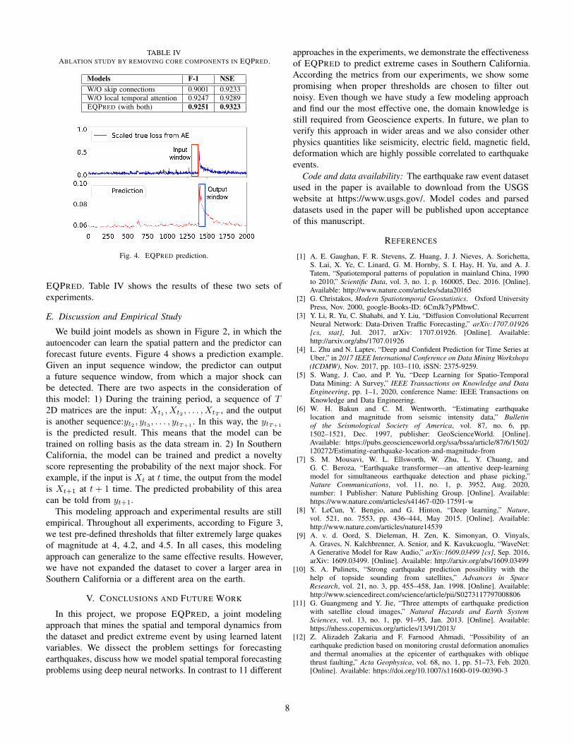
TABLE IVABLATION STUDY BY REMOVING CORE COMPONENTS IN EQPRED.

Models F-1 NSEW/O skip connections 0.9001 0.9233W/O local temporal attention 0.9247 0.9289EQPRED (with both) 0.9251 0.9323

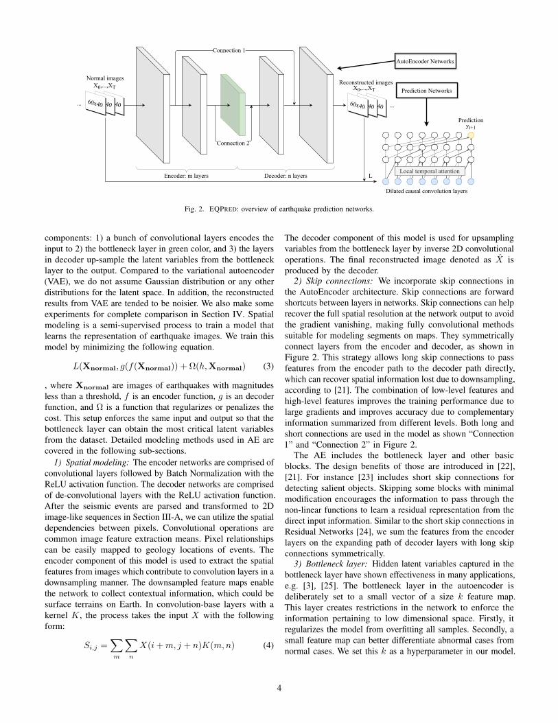
Fig. 4. EQPRED prediction.

EQPRED. Table IV shows the results of these two sets ofexperiments.

E. Discussion and Empirical Study

We build joint models as shown in Figure 2, in which theautoencoder can learn the spatial pattern and the predictor canforecast future events. Figure 4 shows a prediction example.Given an input sequence window, the predictor can outputa future sequence window, from which a major shock canbe detected. There are two aspects in the consideration ofthis model: 1) During the training period, a sequence of T2D matrices are the input: Xt1 , Xt2 , . . . , XtT , and the outputis another sequence:yt2 , yt3 , . . . , ytT+1

. In this way, the ytT+1

is the predicted result. This means that the model can betrained on rolling basis as the data stream in. 2) In SouthernCalifornia, the model can be trained and predict a noveltyscore representing the probability of the next major shock. Forexample, if the input is Xt at t time, the output from the modelis Xt+1 at t+ 1 time. The predicted probability of this areacan be told from yt+1.

This modeling approach and experimental results are stillempirical. Throughout all experiments, according to Figure 3,we test pre-defined thresholds that filter extremely large quakesof magnitude at 4, 4.2, and 4.5. In all cases, this modelingapproach can generalize to the same effective results. However,we have not expanded the dataset to cover a larger area inSouthern California or a different area on the earth.

V. CONCLUSIONS AND FUTURE WORK

In this project, we propose EQPRED, a joint modelingapproach that mines the spatial and temporal dynamics fromthe dataset and predict extreme event by using learned latentvariables. We dissect the problem settings for forecastingearthquakes, discuss how we model spatial temporal forecastingproblems using deep neural networks. In contrast to 11 different

approaches in the experiments, we demonstrate the effectivenessof EQPRED to predict extreme cases in Southern California.According the metrics from our experiments, we show somepromising when proper thresholds are chosen to filter outnoisy. Even though we have study a few modeling approachand find our the most effective one, the domain knowledge isstill required from Geoscience experts. In future, we plan toverify this approach in wider areas and we also consider otherphysics quantities like seismicity, electric field, magnetic field,deformation which are highly possible correlated to earthquakeevents.

Code and data availability: The earthquake raw event datasetused in the paper is available to download from the USGSwebsite at https://www.usgs.gov/. Model codes and parseddatasets used in the paper will be published upon acceptanceof this manuscript.

REFERENCES

[1] A. E. Gaughan, F. R. Stevens, Z. Huang, J. J. Nieves, A. Sorichetta,S. Lai, X. Ye, C. Linard, G. M. Hornby, S. I. Hay, H. Yu, and A. J.Tatem, “Spatiotemporal patterns of population in mainland China, 1990to 2010,” Scientific Data, vol. 3, no. 1, p. 160005, Dec. 2016. [Online].Available: http://www.nature.com/articles/sdata20165

[2] G. Christakos, Modern Spatiotemporal Geostatistics. Oxford UniversityPress, Nov. 2000, google-Books-ID: 6CmJk7yPMbwC.

[3] Y. Li, R. Yu, C. Shahabi, and Y. Liu, “Diffusion Convolutional RecurrentNeural Network: Data-Driven Traffic Forecasting,” arXiv:1707.01926[cs, stat], Jul. 2017, arXiv: 1707.01926. [Online]. Available:http://arxiv.org/abs/1707.01926

[4] L. Zhu and N. Laptev, “Deep and Confident Prediction for Time Series atUber,” in 2017 IEEE International Conference on Data Mining Workshops(ICDMW), Nov. 2017, pp. 103–110, iSSN: 2375-9259.

[5] S. Wang, J. Cao, and P. Yu, “Deep Learning for Spatio-TemporalData Mining: A Survey,” IEEE Transactions on Knowledge and DataEngineering, pp. 1–1, 2020, conference Name: IEEE Transactions onKnowledge and Data Engineering.

[6] W. H. Bakun and C. M. Wentworth, “Estimating earthquakelocation and magnitude from seismic intensity data,” Bulletinof the Seismological Society of America, vol. 87, no. 6, pp.1502–1521, Dec. 1997, publisher: GeoScienceWorld. [Online].Available: https://pubs.geoscienceworld.org/ssa/bssa/article/87/6/1502/120272/Estimating-earthquake-location-and-magnitude-from

[7] S. M. Mousavi, W. L. Ellsworth, W. Zhu, L. Y. Chuang, andG. C. Beroza, “Earthquake transformer—an attentive deep-learningmodel for simultaneous earthquake detection and phase picking,”Nature Communications, vol. 11, no. 1, p. 3952, Aug. 2020,number: 1 Publisher: Nature Publishing Group. [Online]. Available:https://www.nature.com/articles/s41467-020-17591-w

[8] Y. LeCun, Y. Bengio, and G. Hinton, “Deep learning,” Nature,vol. 521, no. 7553, pp. 436–444, May 2015. [Online]. Available:http://www.nature.com/articles/nature14539

[9] A. v. d. Oord, S. Dieleman, H. Zen, K. Simonyan, O. Vinyals,A. Graves, N. Kalchbrenner, A. Senior, and K. Kavukcuoglu, “WaveNet:A Generative Model for Raw Audio,” arXiv:1609.03499 [cs], Sep. 2016,arXiv: 1609.03499. [Online]. Available: http://arxiv.org/abs/1609.03499

[10] S. A. Pulinets, “Strong earthquake prediction possibility with thehelp of topside sounding from satellites,” Advances in SpaceResearch, vol. 21, no. 3, pp. 455–458, Jan. 1998. [Online]. Available:http://www.sciencedirect.com/science/article/pii/S0273117797008806

[11] G. Guangmeng and Y. Jie, “Three attempts of earthquake predictionwith satellite cloud images,” Natural Hazards and Earth SystemSciences, vol. 13, no. 1, pp. 91–95, Jan. 2013. [Online]. Available:https://nhess.copernicus.org/articles/13/91/2013/

[12] Z. Alizadeh Zakaria and F. Farnood Ahmadi, “Possibility of anearthquake prediction based on monitoring crustal deformation anomaliesand thermal anomalies at the epicenter of earthquakes with obliquethrust faulting,” Acta Geophysica, vol. 68, no. 1, pp. 51–73, Feb. 2020.[Online]. Available: https://doi.org/10.1007/s11600-019-00390-3

8

[13] Z. Cui, K. Henrickson, R. Ke, and Y. Wang, “Traffic graph convolutionalrecurrent neural network: A deep learning framework for network-scale traffic learning and forecasting,” IEEE Transactions on IntelligentTransportation Systems, 2019, publisher: IEEE.

[14] Y. Matsubara, Y. Sakurai, W. G. van Panhuis, and C. Faloutsos,“FUNNEL: automatic mining of spatially coevolving epidemics,” inProceedings of the 20th ACM SIGKDD international conference onKnowledge discovery and data mining, ser. KDD ’14. New York, NY,USA: Association for Computing Machinery, Aug. 2014, pp. 105–114.[Online]. Available: https://doi.org/10.1145/2623330.2623624

[15] W. Lotter, G. Kreiman, and D. Cox, “Deep Predictive Coding Networksfor Video Prediction and Unsupervised Learning,” in InternationalConference of Learning Representations (ICLR), Feb. 2017, arXiv:1605.08104. [Online]. Available: http://arxiv.org/abs/1605.08104

[16] C. Finn, I. Goodfellow, and S. Levine, “Unsupervised Learningfor Physical Interaction through Video Prediction,” arXiv:1605.07157[cs], Oct. 2016, arXiv: 1605.07157. [Online]. Available: http://arxiv.org/abs/1605.07157

[17] N. Laptev, J. Yosinski, L. E. Li, and S. Smyl, “Time-series ExtremeEvent Forecasting with Neural Networks at Uber,” p. 5.

[18] X. Geng, Y. Li, L. Wang, L. Zhang, Q. Yang, J. Ye, and Y. Liu,“Spatiotemporal Multi-Graph Convolution Network for Ride-HailingDemand Forecasting,” in Proceedings of the AAAI Conference on ArtificialIntelligence, vol. 33, 2019, pp. 3656–3663.

[19] S. Hochreiter and J. Schmidhuber, “Long short-term memory,” Neuralcomputation, vol. 9, no. 8, pp. 1735–1780, 1997.

[20] Q. Wang, Y. Guo, L. Yu, and P. Li, “Earthquake Prediction Based onSpatio-Temporal Data Mining: An LSTM Network Approach,” IEEETransactions on Emerging Topics in Computing, vol. 8, no. 1, pp. 148–158, Jan. 2020, conference Name: IEEE Transactions on Emerging Topicsin Computing.

[21] K. He, X. Zhang, S. Ren, and J. Sun, “Identity Mappings in DeepResidual Networks,” in Computer Vision – ECCV 2016, ser. LectureNotes in Computer Science, B. Leibe, J. Matas, N. Sebe, and M. Welling,Eds. Cham: Springer International Publishing, 2016, pp. 630–645.

[22] ——, “Deep Residual Learning for Image Recognition,” in 2016 IEEEConference on Computer Vision and Pattern Recognition (CVPR). LasVegas, NV, USA: IEEE, Jun. 2016, pp. 770–778. [Online]. Available:http://ieeexplore.ieee.org/document/7780459/

[23] Q. Hou, M.-M. Cheng, X. Hu, A. Borji, Z. Tu, andP. H. S. Torr, “Deeply Supervised Salient Object DetectionWith Short Connections,” 2017, pp. 3203–3212. [Online].Available: https://openaccess.thecvf.com/content_cvpr_2017/html/Hou_Deeply_Supervised_Salient_CVPR_2017_paper.html

[24] J. Long, E. Shelhamer, and T. Darrell, “Fully ConvolutionalNetworks for Semantic Segmentation,” 2015, pp. 3431–3440. [Online].Available: https://www.cv-foundation.org/openaccess/content_cvpr_2015/html/Long_Fully_Convolutional_Networks_2015_CVPR_paper.html

[30] D. N. Moriasi, J. G. Arnold, M. W. Van Liew, R. L. Bingner, R. D.Harmel, and T. L. Veith, “Model evaluation guidelines for systematicquantification of accuracy in watershed simulations,” Transactions of theASABE, vol. 50, no. 3, pp. 885–900, 2007, publisher: American societyof agricultural and biological engineers.

[25] L. Dong, Y. Gan, X. Mao, Y. Yang, and C. Shen, “Learning DeepRepresentations Using Convolutional Auto-Encoders with SymmetricSkip Connections,” in 2018 IEEE International Conference on Acoustics,Speech and Signal Processing (ICASSP), Apr. 2018, pp. 3006–3010,iSSN: 2379-190X.

[26] J. Yan, L. Mu, L. Wang, R. Ranjan, and A. Y. Zomaya,“Temporal Convolutional Networks for the Advance Prediction ofENSO,” Scientific Reports, vol. 10, no. 1, p. 8055, May 2020,number: 1 Publisher: Nature Publishing Group. [Online]. Available:https://www.nature.com/articles/s41598-020-65070-5

[27] A. Borovykh, S. Bohte, and C. W. Oosterlee, “ConditionalTime Series Forecasting with Convolutional Neural Networks,”arXiv:1703.04691 [stat], Sep. 2018, arXiv: 1703.04691. [Online].Available: http://arxiv.org/abs/1703.04691

[28] A. Vaswani, N. Shazeer, N. Parmar, J. Uszkoreit, L. Jones, A. N. Gomez,\. Kaiser, and I. Polosukhin, “Attention is all you need,” in Advances inneural information processing systems, 2017, pp. 5998–6008.

[29] H. Hao, Y. Wang, Y. Xia, J. Zhao, and F. Shen, “TemporalConvolutional Attention-based Network For Sequence Modeling,”arXiv:2002.12530 [cs], Mar. 2020, arXiv: 2002.12530. [Online].Available: http://arxiv.org/abs/2002.12530

[31] R. H. McCuen, Z. Knight, and A. G. Cutter, “Evaluation of theNash–Sutcliffe Efficiency Index,” Journal of Hydrologic Engineering,vol. 11, no. 6, pp. 597–602, Nov. 2006, publisher: American Society ofCivil Engineers. [Online]. Available: https://ascelibrary.org/doi/abs/10.1061/%28ASCE%291084-0699%282006%2911%3A6%28597%29

[32] M. Abadi, P. Barham, J. Chen, Z. Chen, A. Davis, J. Dean, M. Devin,S. Ghemawat, G. Irving, M. Isard, M. Kudlur, J. Levenberg, R. Monga,S. Moore, D. G. Murray, B. Steiner, P. Tucker, V. Vasudevan, P. Warden,M. Wicke, Y. Yu, and X. Zheng, “TensorFlow: A System for Large-ScaleMachine Learning,” in 12th USENIX Symposium on Operating SystemsDesign and Implementation (OSDI 16), 2016, pp. 265–283. [Online].Available: https://www.usenix.org/conference/osdi16/technical-sessions/presentation/abadi

[33] J. Rojo, R. Rivero, J. Romero-Morte, F. Fernández-González, andR. Pérez-Badia, “Modeling pollen time series using seasonal-trenddecomposition procedure based on LOESS smoothing,” Internationaljournal of biometeorology, vol. 61, no. 2, pp. 335–348, 2017, publisher:Springer.

[34] X. Shi, Z. Chen, H. Wang, D.-Y. Yeung, W.-k. Wong, and W.-c.Woo, “Convolutional LSTM Network: A Machine Learning Approachfor Precipitation Nowcasting,” in Advances in Neural InformationProcessing Systems 28, C. Cortes, N. D. Lawrence, D. D. Lee,M. Sugiyama, and R. Garnett, Eds. Curran Associates, Inc.,2015, pp. 802–810. [Online]. Available: http://papers.nips.cc/paper/5955-convolutional-lstm-network-a-machine-learning-approach-for-precipitation-nowcasting.pdf

[35] D. P. Kingma and M. Welling, “Auto-Encoding Variational Bayes,”arXiv:1312.6114 [cs, stat], Dec. 2013, arXiv: 1312.6114. [Online].Available: http://arxiv.org/abs/1312.6114

9