spatiotemporal models for data-anomaly detection in...
TRANSCRIPT

Spatiotemporal Models for Data-AnomalyDetection in Dynamic Environmental MonitoringCampaigns
Ethan W. Dereszynski and Thomas G. DietterichDepartment of Electrical Engineering and Computer ScienceOregon State University{dereszet,tgd}@eecs.oregonstate.edu
The ecological sciences have benefited greatly from recent advances in wireless sensor technologies.These technologies allow researchers to deploy networks of automated sensors, which can monitora landscape at very fine temporal and spatial scales. However, these networks are subject toharsh conditions, which lead to malfunctions in individual sensors and failures in network com-munications. The resulting data streams often exhibit incorrect data measurements and missingvalues. Identifying and correcting these is time-consuming and error-prone. We present a methodfor real-time automated data quality control (QC) that exploits the spatial and temporal corre-lations in the data to distinguish sensor failures from valid observations. The model adapts toeach deployment site by learning a Bayesian network structure that captures spatial relationshipsbetween sensors, and it extends the structure to a dynamic Bayesian network to incorporate tem-poral correlations. This model is able to flag faulty observations and predict the true values ofthe missing or corrupt readings. The performance of the model is evaluated on data collected bythe SensorScope Project. The results show that the spatiotemporal model demonstrates clear ad-vantages over models that include only temporal or only spatial correlations, and that the modelis capable of accurately imputing corrupted values.
Categories and Subject Descriptors: I.2.6 [Artificial Intelligence]: Learning—Parameter learn-ing; I.5.1 [Pattern Recognition]: Models—Statistical ; structural; G.3 [Mathematics of Com-puting]: Probability and Statistics—Distribution functions; Markov processes; multivariate statis-tics
General Terms: Algorithms, Reliability, VerificationAdditional Key Words and Phrases: Anomaly detection, Bayesian modeling, environmental mon-itoring, quality control, wireless sensor networks
1. INTRODUCTION
The increasing availability (coupled with decreased cost) of lightweight, automatedwireless sensor technologies is changing the way ecosystem scientists collect and dis-
Ethan W. Dereszynski and Thomas G. Dietterich, School of Electrical Engineering and ComputerScience, 1148 Kelley Engineering Center, Oregon State University, Corvallis, OR 97331-5501.This work was supported under the National Science Foundation (NSF) Ecosystem InformaticsIGERT (grant number DGE-0333257) and funding from the EPFL.Permission to make digital/hard copy of all or part of this material without fee for personalor classroom use provided that the copies are not made or distributed for profit or commercialadvantage, the ACM copyright/server notice, the title of the publication, and its date appear, andnotice is given that copying is by permission of the ACM, Inc. To copy otherwise, to republish,to post on servers, or to redistribute to lists requires prior specific permission and/or a fee.© 20YY ACM 0000-0000/20YY/0000-0001 $5.00
ACM Journal Name, Vol. V, No. N, Month 20YY, Pages 1–40.

2 · E. Dereszynski and T. Dietterich
tribute data. Portable sensor stations allow field experts to transport monitoringequipment to sites of interest and observe ecological phenomena at a spatial granu-larity of their choosing. These nonpermanent deployments stand in stark contrastto traditional observatory-like environmental monitoring stations whose initial spa-tial layout remains unchanged over the course of time. However, both approachesare providing researchers with an unprecedented volume of ecological data. Theresultant surge in data has potential to transform ecology from an analytical andcomputational science into a data exploration science [Szalay and Gray 2002].
Temporary sensor deployments, whose durations can range from a single weekto several months, represent a new challenge for data quality control. By nature ofbeing in-situ environmental stations, they are prone to the same technical problemsas long-term deployments, namely damage due to extreme weather, transmissionerrors and loss of signal, calibration errors, and drastic changes in environmentalconditions. Further, it is important to rapidly detect and diagnose a damagedor failing sensor so that it can be repaired. An insufficiently fast diagnosis couldresult in the corruption or loss of data from a given sensor for the duration ofthe deployment; consequently, techniques involving a postmortem analysis of thedata are of little or no value. However, the sheer abundance of data providedby large sensor networks operating at fine time resolutions makes manual analysis(visualizing the data) infeasible for both online and offline quality control. Thisraises the need for efficient automated methods of data “cleaning” that can functionin an online setting and that can readily adapt to dynamic spatial distributions.
The purpose of this article is to provide an example of spatially distributed envi-ronmental monitoring, motivate a need for quality control in this domain throughdocumented examples of sensor failure, and introduce a machine learning approachto automate the data cleaning process. Though we believe our methodology is read-ily extendable to additional environmental phenomena, our work here deals onlywith air temperature data. We propose an adaptive quality control (QC) systemthat exploits both temporal and spatial relationships among multiple environmen-tal sensors at a site. The QC system makes use of a dynamic Bayesian network(DBN, [Dean and Kanazawa 1988]) to correlate sensor readings within a samplingperiod (time step) to readings taken from past sampling periods. Because the setof potential faults is unbounded, it is not practical to approach this as a diagnosisproblem where each fault is modeled separately [Hodge and Austin 2004]. Instead,we employ a general fault model and focus on creating a highly accurate modelof normal behavior, known as the process model. The intuition is that if there isa discrepancy between the current estimate of normal behavior (provided by theprocess model) and the observation taken from the sensor, then the observation islabeled as anomalous. An additional benefit of this approach is that it can imputevalues for the sensor readings during periods of sensor malfunction.
This article is organized as follows. First, we will discuss the current ecologi-cal monitoring campaign, known as SensorScope, that produced the data studiedherein. Second, we describe the nature of the air temperature data and the data-anomaly types encountered, followed by a introduction to hybrid Bayesian networks.Third, we describe our quality control model, including learning the process modeland incorporating a general fault model. Finally, we present the results of theACM Journal Name, Vol. V, No. N, Month 20YY.

Spatiotemporal Models for Data-Anomaly Detection · 3
model applied to temperature data from select SensorScope deployments as well asempirical results on synthetic data. We conclude with a plan for future research.
2. THE SENSORSCOPE SYSTEM
The SensorScope Station, developed at the École Polytechnique Fédérale de Lau-sanne (EPFL) in Switzerland, represents a significant change in traditional toolsfor in-situ data collection and distribution. In place of few, expensive long-term orpermanent monitoring stations deployed sparsely over a heterogeneous spatial area,SensorScope allows field scientists to deploy many light weight, inexpensive stationsat a much higher spatial resolution and monitor at user-specified time granulari-ties. The portability of these stations facilitates dynamic deployments, whereinsensors can be relocated within a deployment to adapt to changing monitoringrequirements.
Component sensors for measuring air temperature, skin (surface) temperature,wind speed, wind direction, humidity, etc. are typically acquired from external man-ufacturers. The SensorScope stations are equipped with a power supply sufficientto host a small set of these sensors (the number dependent on each sensor’s energyrequirement) operating simultaneously, as well as a radio device for communica-tion with nearby stations. Every deployment contains at least one General PacketRadio Service (GPRS) hub that transmits data received from the SensorScope sta-tions to a central server at the EPFL via cellular signal. Once the data reachesthe central server, it is converted from its raw voltage to a value particular to thephenomenon being measured (degrees Celsius in the case of temperatures) via aconversion formula specific to the sensor type. When the data is requested fordownload or plotting via the SensorScope Web site,1 it is filtered automatically bya range checker to remove extreme values associated with sensor malfunctions.
Fig. 1. The Genepi Glacier and FishNet SensorScope deployments (from Google Earth)
Figure 1 (left) shows a 3-D visualization of the Le Genepi Glacier deployment,which was in place from August 27 to November 5 of 2007. The glacial valley,
1http://sensorscope.epfl.ch/index.php/SensorScope_Deployments
ACM Journal Name, Vol. V, No. N, Month 20YY.

4 · E. Dereszynski and T. Dietterich
located approximately 60 kilometers south of the western edge of Lake Geneva,slopes downward toward the northeast and is surrounded by mountains on all othersides. The sensors are placed at an elevation range of 2300 meters to 2500 meters.At the time of the deployment, the northeast corner of the glacier was the onlyarea accessible by cellular signal; therefore, the GPRS (labeled “Base Station 1”)was placed in this location. A total of 16 stations were deployed over the area, whosedimensions can be roughly approximated by a 100 meter by 200 meter rectangle,to allow for a comprehensive analysis incorporating the spatial heterogeneity of therelatively small region.
The right portion of Figure 1 shows a much smaller deployment of six stationsalong a stream, known as the FishNet deployment. The sensors operated from fromAugust 3 to September 4 of 2007. The topographical difference is relatively smallcompared to Le Genepi (the sensors are all located at approximately 600 meters ofelevation), as the deployment was in an agricultural area bordering a forested areato the south. The GPRS station (not shown in the figure) is located approximately100 meters to the west of Station 104, and the length of stream covered by thedeployment is approximately 300 meters.
3. SENSORSCOPE DATA
Each SensorScope station is capable of hosting a changing set of environmentalsensors; hence, there is not a consistent set of phenomena recorded by all stationsacross all deployments. Rather, each station is provided only with those sensorsneeded to measure the variables of interest for a given field campaign and is thenretooled between deployments. As air temperature (the temperature roughly 1.5meters above the surface) is of interest in nearly all campaigns to date, we shallfocus our discussion primarily on this type of data. Air temperature readings aretaken from Sensirion SHT75 sensors mounted on the SensorScope stations [Sensirion2005]. Figures 2 and 3 show two different sets of data streams from the stationsat the FishNet and Le Genepi deployments, respectively. The air temperaturereadings from both sites were sampled at a rate of once every two minutes. Thegraphs show those readings binned and averaged into 10-minute windows.
Nominal air temperature data contains a regular diurnal (day to day) trend thatis dependent on the season and location of the sensor. For example, the FishNethas a more pronounced diurnal signal because the recording period is in the latesummer (August) whereas the the Le Genepi deployment has a suppressed diurnaltrend due to both the time it was observed (October) and its Alpine location. Stormand cloud coverage events occur at irregular intervals but may also suppress diurnalsignal. The FishNet data shows the effect of a storm in days 2 through 4. We havefound the following data-anomaly types present in the air temperature data:
—GPRS Outage. In the case where the GRPS hub becomes inoperative, data forthe entire deployment is lost. The FishNet deployment contains many segmentedperiods of sensor outages among all stations. These outages indicate a failure ofthe GPRS, because they occur simultaneously across all sensor streams. Thefaults are evident between days 15-16 and days 17-20.
—Sensor Outage. A sensor outage occurs when an individual sensor stream is lost.Multiple sensor outages can overlap during a give time period; however, unlike in
ACM Journal Name, Vol. V, No. N, Month 20YY.

Spatiotemporal Models for Data-Anomaly Detection · 5
510
20
data[range, 2]
x101
510
20
data[range, 2]
x102
510
20
data[range, 2]
x103
510
20
data[range, 2]
x104
510
20
data[range, 2]
x105
510
20
data[range, 2]
x106
1 2 3 4 5 6 7 8 9 10 11 12 13 14 15 16 17 18 19 20 21 22 23 24 25 26 27
Air
Tem
pera
ture
(D
egre
es C
elsi
us)
Day Index (From Start of Deployment)
Fig. 2. Air temperature readings from the FishNet SensorScope deployment. Each row representsthe sensor labeled in the corresponding upper right corner. The X axis denotes the day (verticaldashed line depicts midnight) since the deployment began, and the Y axis denotes temperature indegrees ℃. Corresponding station names appear on the right side of the graph next to the streamthey depict.
a GPRS outage, the start, end, and duration of each outage is not synchronized.There are individual sensor outages in the FishNet deployment at stations 101,102, and 103, spanning days 24 and 25.
—Data Anomalies. Data anomalies are characterized as observations from a givensensor that are corrupted due to sensor malfunction. Such anomalous valuesare particularly obvious at station 6 in the Le Genepi deployment (Figure 3),where extremely large temperature values are recorded due to incorrect voltagesgenerated at the sensor. Subtler spikes in temperature occur at station 6 on day41 (Le Genepi) and station 101 on day 17 (FishNet). A flatline in temperatureis created by the temperature sensor reporting a 0-voltage value. The conversionalgorithm maps this value to −1 ℃ value upon storing it into a data base. Anexample of this error is provided in Section 6.2.
Given the correlation between the sensors within a deployment, it is our goal tobe able to identify data anomalies and impute the true temperature values in thecase of both individual sensor outages and sensor malfunctions. Sensor failures thatmanifest themselves as either extraordinarily hot or cold temperatures are simpleto diagnose by means of range checking [Mourad and Bertrand-Krajewski 2002];
ACM Journal Name, Vol. V, No. N, Month 20YY.

6 · E. Dereszynski and T. Dietterich
05
10
data[range, 2]
x2
05
10
data[range, 2]
x3
05
10
data[range, 2]
x4
05
10
data[range, 2]
x6
05
10
data[range, 2]
x7
05
10
data[range, 2]
x8
05
10
data[range, 2]
x10
05
10
data[range, 2]
x11
05
10
data[range, 2]
x12
05
10
data[range, 2]
x20
36 37 38 39 40 41 42
Air
Tem
pera
ture
(D
egre
es C
elsi
us)
Day Index (From Start of Deployment)
Fig. 3. Air temperature readings from one week at the Le Genepi deployment. Each row representsthe sensor labeled in the corresponding upper right corner. The X axis denotes the day (verticaldashed line depicts midnight) since the deployment began, and the Y axis denotes temperature indegrees ℃. Corresponding station names appear on the right side of the graph next to the streamthey depict.
however, malfunctions resulting in flatline values and subtler spikes in temperaturereadings are not detected by extreme value tests. While the values appear anoma-lous in the context of their immediate temporal neighbors, they are not abnormalin the range of temperatures recorded over the full duration of the deployment.
4. HYBRID BAYESIAN NETWORKS
Our probabilistic model of the air temperature domain is a conditional linear-Gaussian network, also known as a hybrid network because it contains both con-tinuous and discrete variables [Lauritzen and Wermuth 1989; Murphy 1998; Pearl1988]. For the sake of computational convenience, we will restrict our networks sothat discrete-valued variables do not have continuous-valued parents and so thatall continuous-valued variables are modeled as Gaussians.
In this section, we describe how the probability distributions for continuous-valued variables are parameterized. We consider three cases: (a) continuous vari-ables with discrete parents, (b) continuous variables with continuous parents, and(c) continuous variables with a mix of discrete and continuous parents.ACM Journal Name, Vol. V, No. N, Month 20YY.

Spatiotemporal Models for Data-Anomaly Detection · 7
4.1 Continuous Variables with Discrete Parents
Consider a single continuous variable, X. For every possible instantiation of valuesfor the discrete parents of X, X takes on a Gaussian distribution with separatevalues for µ and σ2. For example, if X has a single Boolean parent, Y = y ∈{true, false}, then the conditional probability table (CPT) of X would containtwo entries: P (X|y = true) ∼ N
(µt, σ
2t
)and P (X|y = false) ∼ N
(µf , σ
2f
). In
general, let Y = {Y1, Y2, ..., Yn} denote the set of discrete parents of the continuousvariable X. Further, let |Y| = |Y1| × |Y2| × ... × |Yn| be the total size (numberof possible instantiations) of Y. Then, we specify the CPT of X with the |Y|dimensional vector, ~µ =
⟨µ1, µ2, ..., µ|Y|
⟩. Similarly, we specify the set of variances
of X, depending on the parent configuration, as the vector ~σ2 =⟨σ2
1 , σ22 , ..., σ
2|Y|
⟩.
Figure 4 (left) contains an example with binary discrete variables.
X
Y2Y1 Yi Yn-1 Yn… … yi P(Yi=y)true pfalse 1-p
Y1 Y2 …. Yn μ σ2
true true true true μ1 σ21
true true …. false μ2 σ22
… ... false false … …false false false false μ2n σ2
2n
Y
X
Zy P(Y=y)true pfalse 1-p
),(~ 2zzNZ σµ
Y P(X|Y=y, Z=z)true ~N(μ1,x+ w1,z * z, σ2
1)false ~N(μ2,x+ w2,z * z, σ2
2)
Fig. 4. Left: Conditional Gaussian Bayesian Network. Right: Conditional Linear-GaussianBayesian Network
4.2 Continuous Variables with Continuous Parents
Consider a single continuous variable, X, but now with m continuous-valued par-ents. For each continuous-valued parent, Zi ∈ Z = {Z1, Z2, ..., Zm}, X has a weight,wi, such that mean of X is calculated as:
µx = ε+m∑i=1
wizi, (1)
where zi is the value of the parent random variable, Zi, and ε is X’s “interceptterm” in the linear regression formula. An essential requirement for computationaltractability is that the variance of X is specified by a single σ2 parameter andwhich is not conditioned on the parents. Note that this conditional distributionhas exactly the same form as a linear regression model.
4.3 Continuous Variables with a Mix of Discrete and Continuous Parents
If a variable has a mix of continuous and discrete parents, we employ a distinct linearGaussian distribution for each combination of values of the discrete parents. Thisis known as a Conditional Linear Gaussian (CLG) model. Let X be a continuousvariable with a set of discrete parents, Y, and continuous parents, Z. Then X has a
ACM Journal Name, Vol. V, No. N, Month 20YY.

8 · E. Dereszynski and T. Dietterich
separate mean, variance, and set of regression weights for each possible instantiationof Y. We specify a CLG variable by a mean vector, ~µ =
⟨µ1, µ2, ..., µ|Y|
⟩, a variance
vector, ~σ2 =⟨σ2
1 , σ22 , ..., σ
2|Y|
⟩, and a |Y| × |Z| regression matrix:w1,1 w1,2 ... w1,|Z|w2,1 w2,2 ... w2,|Z|w...,1 w...,2 ... w...,|Z|w|Y|,1 w|Y|,2 ... w|Y|,|Z|
. (2)
Figure 4 (right) contains a CLG network with a continuous variable having onediscrete and one continuous parent.
5. DEVELOPING A SPATIOTEMPORAL PROCESS MODEL
In the following sections, we describe our process model as the combination of twoindividual pieces: the spatial component that represents the relationships amongall sensors within a deployment for a given time slice, and a temporal componentthat captures the transition dynamics from one time period (10-minute interval)to the next. The complete process model is represented as a Dynamic BayesianNetwork [Dean and Kanazawa 1988], in which the task of quality control is achievedby inferring the most likely state of the sensors given the current temperatureobservations and those of the immediate past. The procedure for building thecomplete quality control model is summarized in Table I.
5.1 Structure Learning and the Spatial Component
As the geographical layout of stations changes with each deployment, it is desir-able to have the QA routines autonomously learn the spatial relationships for eachnew deployment from the observed data. To this end, we apply Bayesian networkstructure learning algorithms to learn the set of conditional-independence relation-ships among sensors at a given deployment. Recall that though each SensorScopestation is capable of monitoring several environmental variables according to thetype and number of sensors it is hosting, we focus our work to air temperaturedata for purposes of site-to-site continuity and ignore other data types. Further,we assume that each set of air temperature observations corresponding to a single10-minute period is generated from a multivariate Gaussian distribution, and thusa sample from a deployment containing n SensorScope stations is generated froman n-dimensional multivariate Gaussian. Our goal then is to learn the elements ofthe covariance matrix that determine how each dimension (each sensor in a deploy-ment) relates to the others. Our assumptions facilitate the application of a measureknown as BGe (Bayesian metric for Gaussian networks having score equivalence,developed by Geiger and Heckerman [1994]) as a scoring metric for candidate net-works. We summarize the scoring metric, but ask the interested reader to see theaforementioned reference for further details.
A Bayesian network over n Gaussian distributed variables has a joint distributionequal to a n-dimensional multivariate Gaussian. The network structure is referredto as a sparse representation of the multivariate distribution. “Sparse” in thiscontext means that the representative network may not directly correlate eachvariable with all other variables; in graphical terms, less than n(n−1)
2 edges (theACM Journal Name, Vol. V, No. N, Month 20YY.
Spatiotemporal Models for Data-Anomaly Detection · 9
maximum amount of edges for an acyclic graph) are sufficient to represent thecovariance structure among n variables. In general, a lesser degree of connectivityin the graph structure will decrease the time required to perform inference in themodel and reduce the number of parameters to fit once the structure is determined.
The BGe metric assumes the existence of a prior linear Gaussian network whosefull joint distribution represents an initial estimate of the true distribution fromwhich the observations are drawn. This Bayesian network can either be knowledge-engineered by domain experts with information about the deployment or con-structed ad hoc in cases where specific domain knowledge is absent. Geiger andHeckerman parameterize the unknown generative, multivariate distribution with amean vector, ~m, and precision matrix, W = Σ−1. The prior joint distribution onthese parameters is assumed to be a normal-Wishart. Under these assumptions,the joint posterior distribution, given a data set D (containing multivariate ob-servations ~x1, ~x2, ..., ~xl, each of n dimensions), over ~m and W can be divided intothe conditional distribution P (~m|W ) and the marginal P (W ). The conditionaldistribution of P (~m|W ) is given as a multivariate normal
P (~m|W ) ∼ N
(~µl =
v~µ0 + lX̄l
v + l, (v + l)W
)(3)
where v encodes the strength of the prior in terms of an equivalent number of“prior” observations and l is the number of “new” observations in the data set D.The posterior of W is distributed itself as a Wishart (α+ l, Tl), where α specifiesthe degrees of freedom the Wishart distribution (for this reason, α ≥ n must besatisfied). X̄l and Sl are the sample mean and covariance of D, and ~µ0 and Σ0 arethe mean vector and covariance of the prior network structure. The matrices Tland T0 are calculated as
Tl = T0 + Sl +vl
v + l
(~µ0 − X̄l
) (~µ0 − X̄l
)′ (4)
T0 = Σ0v (α− n− 1)
v + 1. (5)
T0 is the precision matrix of the of the prior marginal distribution on W (beforethe observed data D is introduced), given as P (W ) ∼ Wishart (α, T0). The BGemetric scores the likelihood of an hypothesized network structure Bs given a dataset D and the prior ξ as
P (D|Bs, ξ) =n∏
i=1
P (Dxi,Πi |Bcs, ξ)
P (DΠi |Bcs, ξ)
, (6)
where P (Dxi,Πi |Bcs, ξ) is the local score of the data relevant only to variable, xi,
and its parents, Πi. Specifically, we keep only those rows and columns of theT0 and Tl that correspond to variables in xi ∪ Πi in the case of the numeratorin (6). Similarly for the denominator, we keep only those rows and columns inT0 and Tl corresponding to the variables in Πi. The term Bc
s represents a fullyconnected Gaussian Network with edges among all variables. Both the numerator
ACM Journal Name, Vol. V, No. N, Month 20YY.

10 · E. Dereszynski and T. Dietterich
and denominator in (6) are calculated as follows:
P (D|Bs, ξ) = (2π)−nl2
(v
v + l
)n2 c (n, α)
c (n, α+ l)|T0|
α2 |Tl|−
α+l2 (7)
c (n, α) =
[2nα2 π
n(n−1)4
n∏i=1
Γ
(α+ 1− i
2
)]−1
(8)
To score an entire network, the expression in (6) must be evaluated or, equivalently,the expression in (7) must be evaluated for each variable in the domain and theneach resultant value multiplied together. In the case of a nonuniform prior overnetwork structures, an additional weighting of P (Bs|ξ) should be factored into (6).
Provided with a scoring metric for Linear-Gaussian Bayesian Networks, we im-plement a simple hill-climbing algorithm to find a good structure for the networks.The algorithm is initialized with a prior network structure, then it takes one ofthe following actions: (1) add an arc between variables xi and xj if no arc existedalready; (2) remove an existing arc between two variables; or (3) reverse an existingarc between two variables. All three options are undertaken with the constraintthat the resulting structure must remain acyclic. Each of the possible networks cre-ated by taking one of the these actions is evaluated using the BGe metric, and theaction resulting in the highest scoring network is taken. The resultant network thenbecomes the initialization point for another application of this hill-climbing search.The process is repeated until taking a single action (adding, removing, or revers-ing an arc) creates no increase in the score, in which case an optimum has beenreached. Unfortunately, this hill-climbing methodology is subject to local optima,and so the final network is perturbed. This perturbation is achieved by examiningevery existing edge in the current structure and, with some probability, removingthe edge, reversing the direction of the edge (pending no cycle is created), or makingno change. In cases where no edge exists between two variables, we consider addingan edge (pending no introduced cycle) or taking no action. The complete algorithmhalts after performing a user-specified number of perturbations/restarts, and thethe best-scoring network is returned. We outline the aforementioned hill-climbingalgorithm in Algorithm 1.
It is important to note that structure returned from this hill-climbing search maynot be unique relative to its score. The BGe metric demonstrates a property knownas Score Equivalence, which means that it scores network structures belonging to thesame Markov Equivalence Class (MEC) equally. An MEC is the set of graphs thatrepresent the same set of conditional independence relationships between variables.Moreover, the algorithm described above only returns the structure of the network(i.e., the set of parent-child arcs); it does not compute the parameter values for eachvariable (means, variances, and regression weights). In Section 5.4, we describe howwe arrive at these values by computing the Maximum Likelihood Estimates (MLE)for each parameter directly from the data set, D.
The BGe metric is considered a local scoring function because of its decom-position into summing over of node child/parent configurations. Specifically, if weconsider taking the log likelihood of the probability in (6), we arrive at the followingsummation:ACM Journal Name, Vol. V, No. N, Month 20YY.

Spatiotemporal Models for Data-Anomaly Detection · 11
Algorithm 1 Hill-climbing with BGe Metric1: Input: An initial Bayesian Network: Binit
2: Input: Number of perturbations to perform: pturb3:4: CurrentScore = BGe (Binit)5: CurrentNet = Binit
6: BestScore = BGe(Binit)7: BestNet = Binit
8: for i = 1 to pturb do9: LastScore = −∞
10: while CurrentScore > LastScore do11: LastScore = CurrentScore12: AddNet = AddArc(CurrenNet)13: RemNet = RemoveArc(CurrentNet)14: RevNet = ReverseArc(CurrentNet)15: NextNet = argmaxnet [BGe(AddNet), BGe(RemNet), BGe(RevNet)]16: if BGe(NextNet) > CurrentScore then17: CurrentScore = BGe(NextNet)18: CurrentNet = NextNet19: end if20: end while21: if CurrentScore > BestScore then22: BestScore = CurrentScore23: BestNet = CurrentNet24: end if25: CurrentNet = Perturb(CurrentNet)26: CurrentScore = BGe(CurrentNet)27: end for28: return BestNet
logP (D|Bs, ξ) =n∑
i=1
[logP (Dxi,Πi |Bcs, ξ)− logP (DΠi |Bc
s, ξ)]. (9)
We can then compute the log likelihood equivalent of expression Equation 7 tocompute the terms within the summation.
logP (D|Bs, ξ) = log
[(2π)
−nl2
(v
v + l
)n2 c (n, α)
c (n, α+ l)|T0|
α2 |Tl|−
α+l2
](10)
=
[−nl
2log (2π)
]+
[n
2log
(v
v + l
)](11)
+ [log c (n, α)− log c (n, α+ l)] +[α
2log |T0|
](12)
+
[−α+ l
2log |Tl|
](13)
ACM Journal Name, Vol. V, No. N, Month 20YY.

12 · E. Dereszynski and T. Dietterich
Once in summation form, it becomes clear that computing the BGe score for anentire network is only necessary for the initial prior network, Binit. Each subsequentchange in the network structure by adding, removing, or reversing an arc onlyrequires a modification of some factor in the score in (9). For example, if weadd an arc from variable xi to xj , then only the parent set of xi has changed;consequently, we only need to recompute the ith term in (9). The score for theresulting network would be the original network score minus the original ith term(the one not including xj as a parent) plus the new ith term (the one including xjas a parent).
Figure 5 contains a learned structure for the FishNet deployment. The initialprior network assumed complete independence among all six sensor stations atthe site and placed a standard Normal distribution over all sensors (mean of 0and variance of 1.0). The training set is constructed from observations from theSensorScope stations themselves. As we have no ground-truth data for the truetemperature variables (Xi’s), we consider those observations not excluded by thewebsite range-checker or representative of a flatline sensor failure (i.e., consecutive-1 ℃ values) to be the “true” temperature values. The structure was learned usingdata from the first half of the deployment; however, the training set was limited toonly those observations where all sensors reported a value. If a sample missed atleast 1 observation (one sensor failed to report within the 10-minute window), thenit was rejected.
X103
X102
X101
X105
X106
X104
Fig. 5. Left: Top-down view of the FishNet Deployment. Right: Learned dependency relationshipsamong the six sensor stations at the deployment.
5.2 Incorporating a Temporal Model
The spatial model, learned from the methods described in the previous section,captures much of the correlative relationship among multiple sensors within a givendeployment; however, the model suffers from some significant drawbacks. Foremost,the spatial model ignores the transition dynamics present in ecological data – asingle sample taken from all sensors in a time step is considered independent ofall temporally nearby samples (the sample taken 10 minutes ago, 20 minutes ago,etc.). Many types of ecological data are highly autocorrelated. In the case of airtemperature, the diurnal cycle and seasonal cycle mean that data observed 24 hoursand 365 days in the past, respectively, tend to correlate with data observed now.ACM Journal Name, Vol. V, No. N, Month 20YY.

Spatiotemporal Models for Data-Anomaly Detection · 13
Because we generally do not know (or cannot observe due to limited deploymentdurations) the existence of all cycles in the data a priori, we implement only afirst-order Markov relationship in the process model to insure that all stationstransition from the current observation period (10 minutes, for example) to thenext in a consistent manner. This is achieved through the introduction of a parentlag variable for each “true” temperature variable in the spatial model. The lagvariables capture the state of the process in the last time step.
The addition of a Markovian lag changes our model from a static Bayesian net-work into a dynamic Bayesian network. Conceptually, we can now imagine ourlearned spatial model being repeatedly “stamped-out” over the course of l sam-ples in our database. Each stamp, or layer, contains the learned Bayesian networkrepresenting the spatial relationships in addition to a lag variable for each sensor.Figure 6 depicts the temporal model appended to the learned spatial model for theFishNet deployment.
As mentioned in Section 5.1, the spatial component returned by our hill-climbingsearch is not a unique representation of the set of conditional independencies be-tween the temperature variables; it belongs to a Markov Equivalence Class. How-ever, once we append our temporal model to each network in the MEC, the resultantmodels may no longer belong to the same class. To choose the best candidate net-work for the spatial model, we generate all members of this set by using an approachdescribed by Andersson et al. [1995]. Given a directed acyclic graph (DAG), theiralgorithm returns an essential graph that represents the equivalence class and hasdirected or undirected edges in place of all edges in the input graph. Undirectededges represent relationships between variables that can be reversed (parent be-comes the child and visa versa) without changing the overall set of conditionalindependence relationships. We input our learned spatial model to create the es-sential graph representing its MEC. We consider all permutations of orientationsfor the undirected edges in the essential graph such that no cycles are introduced.For each DAG generated in this fashion, we append a set of lag variables, fit theparameters of the combined model as described in Section 5.4, and score the likeli-hood of the training data given this new network. We choose the spatial model thatyields the highest data likelihood when combined with the temporal component.
X103
X102
X101
X105
X106
X104
X103
X102
X101
X105
X106
X104
Time t-1 Time t
Fig. 6. Time slices are designated by the dashed rectangles. Lag variables are appended for eachsensor in the deployment, representing the state of the process in the last time slice.
The first-order Markovian assumption means that we need only consider the stateACM Journal Name, Vol. V, No. N, Month 20YY.
14 · E. Dereszynski and T. Dietterich
of the process in the previous time step and observations in the current time slicewhen inferring the posterior distribution over the current state of the process. Forexample, to compute the posterior of X104 at time t from the DBN in Figure 6, weneed only the distribution over the previous time step and any observations in thecurrent time step
P(Xt
104|X1101, X
2101, ..., X
t−1101 , X
1102, X
2102, ..., X
t−1102 , ..., X
1106, X
2106, ..., X
t−1106
)(14)
= P(Xt
104|Xt−1101 , X
t−1102 , X
t−1103 , X
t−1104 , X
t−1105 , X
t−1106
)(15)
Each variable in our original network now has one additional parent variable andthus one additional parameter (weight associated with the new parent) to estimate.We can still apply our MLE technique for estimating the new parameter values;however, the training set for this model is now a subset of the training set used forour spatial model. This is because we now must place the additional constraint onour training data that it consists of contiguous pairs (two consecutive 10-minuteintervals) where all sensor observations are present. We discuss how we respect thisconstraint in our Experiments and Methodology section.
5.3 Incorporating the Sensor Model
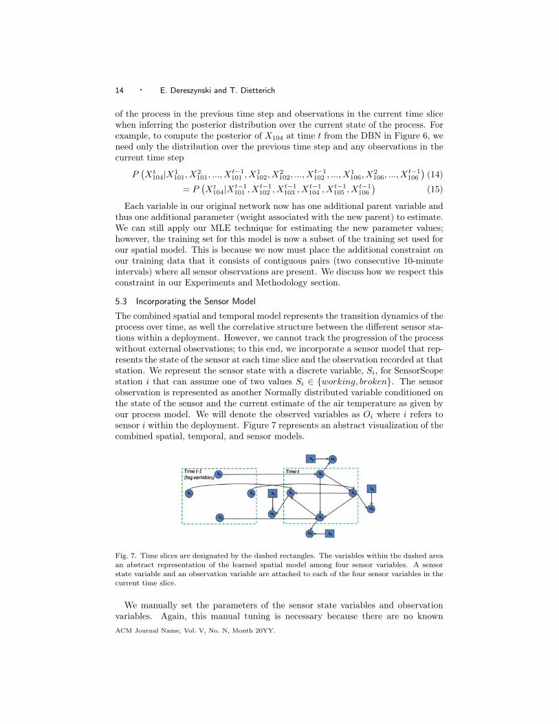
The combined spatial and temporal model represents the transition dynamics of theprocess over time, as well the correlative structure between the different sensor sta-tions within a deployment. However, we cannot track the progression of the processwithout external observations; to this end, we incorporate a sensor model that rep-resents the state of the sensor at each time slice and the observation recorded at thatstation. We represent the sensor state with a discrete variable, Si, for SensorScopestation i that can assume one of two values Si ∈ {working, broken}. The sensorobservation is represented as another Normally distributed variable conditioned onthe state of the sensor and the current estimate of the air temperature as given byour process model. We will denote the observed variables as Oi where i refers tosensor i within the deployment. Figure 7 represents an abstract visualization of thecombined spatial, temporal, and sensor models.
Fig. 7. Time slices are designated by the dashed rectangles. The variables within the dashed areaan abstract representation of the learned spatial model among four sensor variables. A sensorstate variable and an observation variable are attached to each of the four sensor variables in thecurrent time slice.
We manually set the parameters of the sensor state variables and observationvariables. Again, this manual tuning is necessary because there are no knownACM Journal Name, Vol. V, No. N, Month 20YY.
Spatiotemporal Models for Data-Anomaly Detection · 15
labels for the sensor states in any of the SensorScope datasets. For each Si, we setthe P (Si = working) = P (Si = broken) = .5 and for Oi
P (Oi|Si = working,Xi = xi) ∼ N (xi, 0.1) and (16)P (Oi|Si = broken,Xi = xi) ∼ N (.0001xi, 10000.0) . (17)
This parameterization stems from the idea that the sensor state must be able to“explain away” the discrepancy between the observation variable, Oi, and the cur-rent estimate of the true air temperature, Xi. That is, if the sensor is believed to beworking, then the observation value should be equal to that of the process model’sestimate with some small, additional variance (0.1 ℃); contrarily, if the sensor isbelieved to be broken, then the observation has little do with the actual process andso is much noisier (10000.0 ℃ variance). The 0-mean, large variance distributionof the broken state approximates a uniform distribution over the possible range ofobserved sensor values. If we had ground-truth labels for the sensor state in eachobservation, explicitly modeling each fault with a separate distribution would nothelp us identify new anomaly types not seen in the training data. However, we couldestimate P (Si = working) as the ratio of the number of working sensor observationsover the total number of observations (and P (Si = broken) = 1−P (Si = working)).
5.4 Parameter Estimation
Recall that under the assumption of a linear-Gaussian model, a Normally dis-tributed variable, X ∼ N(µx, σ
2x), conditioned on a Normally distributed parent,
Y ∼ N(µy, σ2y), has the following density function (assuming both are univariate):
P (X|Y ) =1
σx√
2πexp− (x− (w1y + µx))
2
2σ2x
(18)
That is, P (X|Y ) ∼ N(µx + w1y, σ2x), where w1 is a scalar weight multiplied with
an input, y, drawn from Y ’s distribution.Once our structure learning algorithm has provided each variable in our domain
with a set of parents (including the temporal lag variables), the MLE approachto estimating the values of the parameters (µi, σ
2i , and wi) reduces to solving a
multiple linear regression problem [Russell and Norvig 2003]. Specifically, we solve
θ̂ =(XTX
)−1
XT ~Y , (19)
where θ̂ represents the mean and associated weights of the target variable (thevariable whose parameters we are currently estimating), X is a matrix containingthe value of the parents of the target variable in the data set across all samples,and ~Y is a vector containing all the values of the target variable corresponding tothe inputs in X.
5.5 Inference
Inference is performed in our models using the Variable Elimination (VE, [Dechter1996]) algorithm adapted for Conditional Linear Gaussian models [Lauritzen 1992;Lauritzen and Wermuth 1989; Murphy 1998]. There are two inference queries madeat each time step, t.
ACM Journal Name, Vol. V, No. N, Month 20YY.

16 · E. Dereszynski and T. Dietterich
Table I. Procedure for Constructing Full QC Model
(1) Begin with initial Bayesian Network structure, Binit, for the input data, D.If no initial network is provided, Binit is a network containing no arcs and eachvariable xi ∈ Binit ∼ N (0, 1.0)
(2) Compute the sample mean and covariance of D, X̄l and Sl.(3) Compute the mean and covariance represented by Binit: ~µ0 and Σ0.(4) Compute T0 and TM using the values from steps (2) and (3) in equations (5)and (4).(5) Perform hill-climbing (Algorithm 1) initialized from Binit. Call the resultantstructure Bpost.(6) Build the Markov Equivalence Set, {Bk|Bk ∈ MEC (Bpost)} and append thetemporal model to each network Bk.(7) Compute MLE parameters for each Bk ∈ MEC (Bpost) from the data, D.(8) Compute Bbest = arg maxBk P (D|Bk).(9) Append Sensor State (Si) and Observation variables (Oi) for each sensorvariable (Xi) in Bbest. The parameters of these variables are manually set.
First, we wish to compute the maximum a posteriori (MAP) assignment of thediscrete sensor variables, ~St, given the set of sensor observations, ~Ot,
P(St
1, St2, ..., S
tn|Ot
1 = ot1, Ot2 = ot2, ..., O
tn = otn
). (20)
This requires marginalization of the the hidden “true” temperatures (continuousvariables) at time t and t − 1. The remaining sensor-state variables (discrete)are contained in a single potential whose distribution is represented by a tablehaving an exponential number of entries. Each entry corresponds to one of the 2n
possible configurations of n sensor-state variables; consequently, construction of thistable occurs in time exponential with the sensor count. The sensor counts in thedeployments discussed herein were not prohibitively large; however, for deploymentscontaining more sensors, we could consider approximate inference algorithms, suchas Gibbs Sampling [Geman and Geman 1984] or other particle filter methods. Thesealgorithms approach the exact solution as the number of samples or particles usedincreases. While each sample can be generated in linear time, the number of samplesrequired to reasonably approximate the true joint posterior may be exponentialin the number of sensors. Alternatively, we could impose a prior on our spatialstructures that would encourage learning disjoint spatial models (i.e. spatial modelswhere one or more of the Xi variables is disconnected from the remainder). In thiscase, exact inference would be exponential in the number of sensors in the largestsubgraph.
Second, we treat the MAP assignment as new evidence for the sensor states attime t and compute the updated estimate of the hidden “true” temperatures, ~Xt,
P(Xt
1, ..., Xtn|St
1 = st1, ..., Stn = stn, O
t1 = ot1, ..., O
tn = otn
). (21)
Because we now observe the sensor states, computing the posterior over the truetemperatures becomes a query over a linear-Gaussian model. Variable EliminationACM Journal Name, Vol. V, No. N, Month 20YY.

Spatiotemporal Models for Data-Anomaly Detection · 17
takes cubic time in the number of sensors for this query and so is tractable toperform exactly. The posterior distribution on the true temperatures is passedforward as a message to be used in inference at time t + 1. The joint posteriordistribution over the true temperature variables can be thought of as an α messagein the forward pass of a filtering algorithm [Rabiner 1990]. If the MAP estimateof the sensors at time t indicates that sensor i is working (Si = working), then weinput its corresponding observation (Oi) for the true temperature’s lag variable attime t+ 1; otherwise, we use the corresponding α message to specify a distributionover the lag’s value. We then repeat this two-step query procedure for time t+ 1.
Our motivation for handling inference in this two-step process is that, in anonline setting, we must make a decision that each sensor at time t is working orbroken rather than postponing this decision and maintaining a “belief state,” thatis, 79% working and 21% broken. Not only is this approximation useful for an onlineQC system, it also exempts us from having to maintain an exact belief state thatincreases in size after each time step. To clarify, the exact belief state at time t wouldbe a 2nt component mixture of n-dimensional multivariate Gaussians. Once we havedetermined the state of each sensor, we need to propagate forward an α messageregarding the true temperatures ~X to time t + 1 (computed in (21)). Thus, ourapproximation is made by considering only the mixture component correspondingto the MAP of the Si variables at each time step.
6. EXPERIMENTS AND METHODOLOGY
Our experiments focus on the validation of our learned spatial models across varyingdeployments and the efficacy of our complete DBN model as a tool for qualitycontrol. We address each issue in turn. We perform the former validation through aseries of hold-one-out prediction tests to determine the relative strength of multiplestations as a predictor for an individual missing station. Second, we provide acomparative analysis of the performance of three different QC models as applied toreal data from the SensorScope project. The three models are the spatial, temporal,and spatiotemporal models already discussed, each augmented with a sensor modelas described in Section 5.3. The experiments reflect the weaknesses and strengthsof each model, and show preliminary justification for pursuing a spatiotemporalapproach. Lastly, we evaluate the performance of our model in terms of type I andtype II error rates. This experiment is performed via the addition of artificial noiseto the original datasets in order to create labels that can be matched against ourpredictions of the sensor variable.
All experiments in this section were performed with a data set spanning from thebeginning of the respective deployment to its end. Because the SensorScope stationsare not necessarily synchronized to sample at the same time, the data was binnedand averaged into 10-minute windows consistent across all stations. A training setand testing set were created for each deployment by roughly splitting the data intohalves, in which the first half (representing the first chronological half) became thetraining data and the second half became the test set. In all experiments, onlytraining samples (10 minute windows) where readings for all of the stations werepresent were used, and so often the training sets are significantly smaller than thetesting sets. For experiments containing a temporal model, only those training
ACM Journal Name, Vol. V, No. N, Month 20YY.

18 · E. Dereszynski and T. Dietterich
samples that had a fully observed preceding sample (the last 10-minute period)were used. Data for the experiments comes from the FishNet and the Grand St.Bernard deployments. Grand St. Bernard was a third deployment located in theGrand St. Bernard Pass between Switzerland and Italy (at an elevation of 2300meters) and was in place from September 13, 2007 to October 26, 2007. All sixsensors were used in the FishNet deployment; however, only a subset comprising 9of the 23 stations were used from the Grand St. Bernard (see Figure 8). Becausewe are only including training samples where all sensor measurements are present,including all stations from the Grand St. Bernard would exclude too many potentialsamples.
Fig. 8. Left: The portion of the Grand St. Bernard deployment on the Italian side of the mountainpass. Right: The Swiss side of the Grand St. Bernard deployment, located approximately 2kilometers east of the Italian deployment. The stations circled in red denote those stations chosenfor purposes of modeling.
6.1 Leave-One-Out Prediction
The leave-one-out experiments are performed by withholding a sensor’s observa-tion and computing the posterior distribution over the hidden sensor value givenall other sensor observations and the learned spatial (Section 5.1) and spatiotempo-ral models (Section 5.2). We report results for the FishNet and Grand St. BernardSensorScope deployments. In both cases, the spatial model is learned and param-eterized using only the first half of the data (approximately 1400 and 440 trainingsamples, respectively).
Once the spatial and spatiotemporal models are trained, we process the testingdata (second half of the collected samples) in an iterative manner. In each iteration,a single observation, representing the measurement taken at one station at one timepoint, is removed. We compute a posterior prediction for the removed value usingthe learned spatial model and the observations from all other stations in the caseof the spatial model, and all other stations in addition to all measurements fromthe previous time step in the case of the spatiotemporal model. We compute themean squared error (MSE) between the predicted value for the withheld observationand its actual value in the test set, as well as the variance in our prediction. LetACM Journal Name, Vol. V, No. N, Month 20YY.

Spatiotemporal Models for Data-Anomaly Detection · 19
t = 1, ..., T denote the time (sample) index, i = 1, ..., n index the “true” temperaturevariable Xi, and xti be the value of the true temperature at station Xi at time t.The MSE and Variance for station Xi is then computed as
MSEi =1
T
T∑t=1
(E [P (Xi|X\Xi)]− xti
)2. (22)
The variance of the posterior estimate of Xi depends only on the set of variablesthat are observed (included in the set X\Xi); not on the exact value of thoseobservations. Thus, we need only examine V ar [P (Xi|X\Xi)] for any one of the tsamples above to determine the variance. The leave-one-out error is also measuredusing cumulative log likelihood (CLL),
CLLi =T∑
t=1
logP (Xi = xti|X\Xi), (23)
and is shown as the dashed horizontal line in Figures 9, 10, and 11. We thenperform a further computation, removing an additional variable’s observation fromthe testing data. We compute the cumulative error over the training data (sum loglikelihood) in predicting our original target variable with one additional sensor’sobservation missing. Using the same notation as above, we compute this as
CLLi,j =T∑
t=1
logP (Xi = xti|X\ {Xi, Xj}). (24)
Each bar in Figures 9, 10, and 11 corresponds to the new CLL value after thevariable Xj has been hidden. The purpose of removing a second variable Xj isto measure the contribution of second variable in predicting the value of the firstremoved variable Xi.
Figure 9 (upper left plot) indicates that station 101 was not only the most difficultto predict (MSE of .56 ℃), but also gained the least from the presence of othersensors. Additionally, removing the observations of station 104 resulted in thelargest increase in error for station 101; however, even this effect was not particularlysignificant in comparison to removing any of the other remaining stations. Thelikely reason for this lack of correlation is due to station 101’s position on thesouth edge of the deployment (Figure 5), near the wooded border. Station 104, itsmost similar station, is also located in close proximity to a wooded, shady region,which may explain its role as the strongest predictor for station 101. This examplehighlights the fact that our “spatial” learning is discovering more correlation thanthose just based on spatial proximity as we might see in a Kriging model [Matheron1963]. Rather, our model is capturing all sources of linear correlation betweensensors at a given time step, without the use of a feature set describing each sensor.
Stations 105 and 106 (bottom center and bottom right plots, respectively) appearto be very highly correlated, as indicated by the dramatic increase in predictionerror when either station is held out while predicting the other. Moreover, we seethat when holding out each station (105 and 106), there is little error in reproducingthe withheld observation given the presence of the other 5 sensors (MSEs of .058 ℃and .074 ℃, respectively). The Sensirion SHT75 documentation reports a measur-
ACM Journal Name, Vol. V, No. N, Month 20YY.

20 · E. Dereszynski and T. Dietterich
x102 x103 x104 x105 x106
050
010
0015
0020
00
MSE: 0.56Var: 0.51
x101 x103 x104 x105 x106
020
040
060
080
010
0012
00
MSE: 0.22Var: 0.13
x101 x102 x104 x105 x106
010
020
030
040
050
060
070
0
MSE: 0.09Var: 0.06
x101 x102 x103 x105 x106
050
010
0015
00
MSE: 0.35Var: 0.40
x101 x102 x103 x104 x106
020
040
060
080
0
MSE: 0.06Var: 0.04
x101 x102 x103 x104 x105
020
040
060
080
010
00 MSE: 0.07Var: 0.04
Err
or (
Cum
ulat
ive
Log
Like
lihoo
d)
Held−out Sensor Variable
Fig. 9. Redundancy Test for FishNet Spatial Model. Dashed line indicates the error in predictingthe individual missing sensor. Each bar along the X axis represents the change in error fromremoving the additional sensor variable corresponding to that bar. The Y axis is the error mea-sured as the cumulative log likelihood over all test cases of the true value given the predicteddistribution.
ing accuracy of ±.35 ℃ in operating conditions of 15.21 ℃ (average temperatureof the FishNet site for the testing period).
Figure 10 conveys a similar analysis performed with nine stations selected fromthe Grand St. Bernard deployment (Figure 8). The top row of bar plots depicts theanalysis of stations 11, 12, and 17, while the bottom row corresponds to stations25, 29, and 31. It is apparent from the plot that stations 17 and 29 are the mostdifficult to predict from the remaining 8 sensors. This stands to reason for station29, for though it is located on the Italian side of the deployment with 25 and 31,it is still separated by a steep hillside dividing the region. We could not ultimatelydiscern the reason for station 17’s discordant behavior from the remaining sites.The Sensirion SHT75 documentation reports a measuring accuracy of ±1.0 ℃ inoperating conditions of 1.83 ℃ (average temperature of the Grand St. Bernard sitefor the testing period).
It is interesting to note in Figure 10 that, in all cases, there exists at least onesensor whose removal actually seems to decrease the amount of error in predictingthe hold-out sensor’s value. This trend suggests that our learned model may haveoverfit the original training data, and thus poorly generalized to the test set. In thecase of air temperature data measured over 1-2 months (especially during seasonaltransitions), data monitored at the beginning of the observation period can differsignificantly from data measured toward the end of the observation period. Thiscompounds the difficulty of our work, as now our underlying assumption of a singlegenerative multivariate distribution creating our training and testing data is nolonger valid. Future work will need to focus on time-series analysis techniques thatcan map the test set to our training set without full knowledge of the trend effectsACM Journal Name, Vol. V, No. N, Month 20YY.

Spatiotemporal Models for Data-Anomaly Detection · 21
x12 x17 x18 x19 x20 x25 x29 x31
050
010
0015
0020
0025
00
MSE: 0.58Var: 0.07
x11 x17 x18 x19 x20 x25 x29 x31
050
010
0015
00 MSE: 0.48Var: 0.08
x11 x12 x18 x19 x20 x25 x29 x31
020
0040
0060
0080
00
MSE: 2.54Var: 0.08
x11 x12 x17 x18 x19 x20 x29 x31
050
010
0015
0020
0025
0030
00 MSE: 0.27
Var: 0.07
x11 x12 x17 x18 x19 x20 x25 x31
010
0020
0030
0040
0050
0060
00
MSE: 5.13Var: 0.21
x11 x12 x17 x18 x19 x20 x25 x29
050
010
0015
0020
0025
00
MSE: 0.22Var: 0.09
Err
or (
Cum
ulat
ive
Log
Like
lihoo
d)
Held−out Sensor Variable
Fig. 10. Redundancy Test for Grand St. Bernard Spatial Model. Dashed line indicates the error inpredicting the individual missing sensor. Each bar along the X-axis represents the change in errorfrom removing the additional sensor variable corresponding to that bar. The Y-axis is the errormeasured as the cumulative log likelihood over all test cases of the true value given the predicteddistribution.
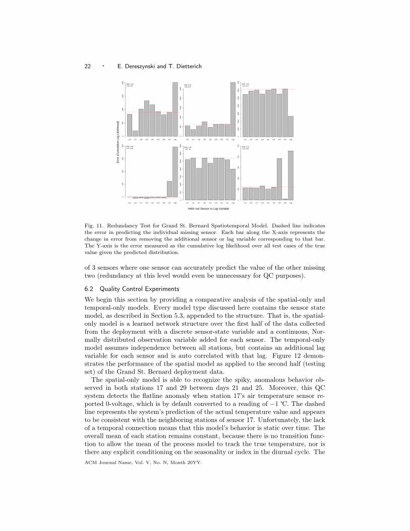
that shape the generative distribution over time.Finally, Figure 11 shows the hold-one-out analysis applied to a spatiotemporal
model learned from the Grand St. Bernard data. Recall that this model is simplythe original spatial model with the relevant lag variables appended to its structure,and the parameters reestimated to account for the additional set of parents. Wenotice that, in all cases, the hold-one-out error decreases with the incorporationof a lag effect. Also significant is that, with the exception of stations 17 and29, the lag effect has the greatest predictive power for every station. This makesintuitive sense, as air temperature is unlikely to change significantly over the courseof 10 minutes (the duration of the lag). Stations 17 and 29 suffer from the sameoverfitting problem in this revised model, as hiding the Markovian variable reduceserror in both cases. In fact, the large magnitude of the gain incurred from hidingthe lag variable from station 17 seems to support the theory that the nature of thecorrelative effect changed drastically between the training and testing periods. Ifit had not, then it is unlikely that the spatiotemporal model would have lent thelag variable such significant weight based on the training data.
In addition to providing some intuition about the values of parameters and net-work structures learned in the spatial component of our QC system, this type ofhold-one-out analysis can be used to identify redundant sensors. For purposes ofquality control, two sensors measuring the same phenomenon (or one able to near-perfectly predict the other’s missing value) is necessary to truly validate recordedobservations; however, for purposes of capturing all the heterogeneity encompassedwithin a site, it may be preferable to relocate any sensor considered redundant.This analysis can be easily generalized to hold-two-out in order to detect clusters
ACM Journal Name, Vol. V, No. N, Month 20YY.
22 · E. Dereszynski and T. Dietterich
x12 x17 x18 x19 x20 x25 x29 x31 Lag
050
010
0015
0020
00
MSE: 0.34Var: 0.07
x11 x17 x18 x19 x20 x25 x29 x31 Lag
050
010
0015
0020
0025
00
MSE: 0.26Var: 0.07
x11 x12 x18 x19 x20 x25 x29 x31 Lag
010
0020
0030
0040
0050
0060
0070
00
MSE: 2.00Var: 0.07
x11 x12 x17 x18 x19 x20 x29 x31 Lag
020
040
060
080
0
MSE: 0.05Var: 0.05
x11 x12 x17 x18 x19 x20 x25 x31 Lag
050
010
0015
0020
0025
0030
0035
00
MSE: 1.98Var: .16
x11 x12 x17 x18 x19 x20 x25 x29 Lag
010
020
030
040
050
0
MSE: 0.10Var: 0.08
Err
or (
Cum
ulat
ive
Log
Like
lihoo
d)
Held−out Sensor or Lag Variable
Fig. 11. Redundancy Test for Grand St. Bernard Spatiotemporal Model. Dashed line indicatesthe error in predicting the individual missing sensor. Each bar along the X-axis represents thechange in error from removing the additional sensor or lag variable corresponding to that bar.The Y-axis is the error measured as the cumulative log likelihood over all test cases of the truevalue given the predicted distribution.
of 3 sensors where one sensor can accurately predict the value of the other missingtwo (redundancy at this level would even be unnecessary for QC purposes).
6.2 Quality Control Experiments
We begin this section by providing a comparative analysis of the spatial-only andtemporal-only models. Every model type discussed here contains the sensor statemodel, as described in Section 5.3, appended to the structure. That is, the spatial-only model is a learned network structure over the first half of the data collectedfrom the deployment with a discrete sensor-state variable and a continuous, Nor-mally distributed observation variable added for each sensor. The temporal-onlymodel assumes independence between all stations, but contains an additional lagvariable for each sensor and is auto correlated with that lag. Figure 12 demon-strates the performance of the spatial model as applied to the second half (testingset) of the Grand St. Bernard deployment data.
The spatial-only model is able to recognize the spiky, anomalous behavior ob-served in both stations 17 and 29 between days 21 and 25. Moreover, this QCsystem detects the flatline anomaly when station 17’s air temperature sensor re-ported 0-voltage, which is by default converted to a reading of −1 ℃. The dashedline represents the system’s prediction of the actual temperature value and appearsto be consistent with the neighboring stations of sensor 17. Unfortunately, the lackof a temporal connection means that this model’s behavior is static over time. Theoverall mean of each station remains constant, because there is no transition func-tion to allow the mean of the process model to track the true temperature, nor isthere any explicit conditioning on the seasonality or index in the diurnal cycle. TheACM Journal Name, Vol. V, No. N, Month 20YY.

Spatiotemporal Models for Data-Anomaly Detection · 23
−10
010
data[range, 2]
| |||||||| ||||||||||||||||||||||||||||||||||| |||||||||||||||||||||||||||||||||||||||||| ||||||||||||| | || |||||| ||||| | ||||||||||||||||||||||||||||||||||||||||||||||||||||||||||||||||| ||||||||||||||||||||||||||||||||||||||||||||||||||||||||||||||||||||||||||||||||||||||||||||||||||||||||||||||||||||| | ||||||||||| ||||||||||||||||||||| ||| ||||||||||||||||||||||||||| |||||||||||||||||||| |||| | |||||||||||||||||||||||||||||||||||||||||||||||||||||||||||| | ||| | || ||| ||
x11
−10
010
data[range, 2]
||||||| ||||| || | | | | ||| |||||||||||||||||||| ||||||||||||||||||||||||||||||||||||||||| || ||||||||||||||||| | ||||||||||| ||||||||||||||||||||| ||||||||||||||||||||||||||| ||||||||||||||||||| |||| | |||||||||||||||||||||||||||||||||||||||||||||||||||||||||||||||| | ||||| |||||||| |||| |||
x12
−10
010
data[range, 2]
|||||||||||||||||||| |||||| | ||| ||||||||||||||||||||||||| |||||||||||||||| ||||||||||||| ||||||| ||||||||||||||||||||||||||||||||||||||||||||||||||||||||||||||| |||||||||||||||||||||||||||||||||||||||||||||||||||||||||||||||||||||||||||||||||||||||||||||||||||||||||||||||||||||| ||||||||||||||||||||||||||||||||||||||||||||||||||||||||||||||||||||||||||||||||||||||||||||||||||||||||||||||| |||||||||||||||||||||||||||||||||||||||||||||||||||||||||||||||||||||||||||||||||||||||||||||||||||||||||||||| |||||||||||||||||||||||||||||||||||||||||||||||||||||||||||||||||||||||||||||||||||||||||||||||||||||||||||||||||||||||||||||||||||||||||||||||||||||||||||||||||||||||||||||||||||||||||||||||||||||||||||||||||||||||||||||||||||||||||||||||||||||||||||||||||||||||||||||||||||||||||||||||||||||||||||||||||||||||||||||||||||||||||||||||||||||||||||||||||||||||||||||||||||||||||||||||||||||||||||||||||||||||||||||||||||||||||||||||||||||||||||||||||||||||||||||||||||||||||||||||||||||||||||||||||||||||||||||||||||||||||||||||||||||||||||||||||||||||||||||||||||||||||||||||||||||||||||||||||||||||||||||||||||||||||||||||||||||| |||||||||||||||||||||||||||| | |||| ||||||||||||||||||||||| ||||||||||||||||||||||||||||||||||| ||||||||||||||||| | || ||||||||||| ||||||||||||||||||||| ||||||||||||||||||||||||||| |||||||||||||||||||| ||||||| |||||||||||||||||||||||||||||||||||||||||||||||||||||||||||| |||| ||| ||| |||||||
x17
−10
010
data[range, 2]
| || ||||| | || ||| |||||| | |||| |||||||||| | | |||| | |||||||| ||||||||||||||||||||||||||||||||||||||||| || ||||||||||||||||||||| | ||||||||||| ||||||||||||||||||||| ||||||||||||||||||||||||||| ||||||||||||||||||| ||||| | ||||||||||||||||||||||||||||||||||||||||||||||||||||||||||||| |||||||| ||| |||
x18
−10
010
data[range, 2]
| | |||| ||||| ||| ||||||||| ||||||||||| |||||||||| |||||||||||||||||||| |||||||||||||||| ||||||| ||||||||| |||| | |||||||| || ||||||||||||||||| || |||||||||||||||||||||||||||||||||||||||||||||||||| ||| |||||||||||||||||||||| ||||||||||||||||||||||||||||||||||||||||||||||||||||||||||||||||||| ||||||||||||||||||||||||| ||||||||||||||||||||||||||| ||||||||||||||||||||| |||||||||| | ||||||||||||||||||||||||||||||||||||||||||||||||||||||||||| ||||| ||||| | ||||
x19
−10
010
data[range, 2]
|| | |||| | ||||||||| ||| | | |||||||||||||| |||||||||||||||||||| ||||||||||||||||| |||||| | ||||||||||| || ||||||||||||||||||||||||||||||||||||||||||||| || ||||||||||||||| || ||||||||||||||||||||||||||||||||||||||||||| || ||||||||||||||||||||||||||||||||||||| | ||||||||||| |||||||||||||||||||||||||||||| ||||||||||||||||||||||||||| |||||||||||||||||||||||||||||||||||||||||||||||||||||| | |||||||||||||||||||||||||||||||||||||||||||||||||||||||||||||||||||||||||||||||||||||||||||||||| | |||||||||
x20
−10
010
data[range, 2]
| |||||||||||||||| ||| | ||| | | || ||||||||||||||||||||||||||||||||||||||||||||||||||||||||||||||||||| ||||||||||| ||||||||||||||||||||| ||||||||||||||||||||||||||| ||||||||||||||||||| ||| | |||||||||||||||||||||||||||||||||||||||||||||||||||||| | |||| ||||||||| | ||| ||||||||||||||||||||||||||||||||||||||||||||||||||||||||||||||||||||||||||||||||||||||||||||||||||||||||||||||||||||||||||||||||||||||||||||||||||||||||||||||||||||||||||||||||||||||||||||||||||||||||||||||||
x25
−10
010
data[range, 2]
| |||||||||||||||||||||||||||||||||||||||||||||||||||||||||||||||||||||||||||||||||||||||||||||||||||||||||||||||||||||||||||||| |||||||| | |||||||||||||||||||||||||||||||||||||||||||||||| | | || || ||| ||| | | ||||| | |||||||||||||||||||||||||||||||||||||||||||||||||||||||||||||||||||||||||| ||||||||||||||||||||||||||||||||||||||||||||||||||||||||||||||||||||||||||||||||||||||||||||||||||||||||||||||||||||||||||||||||||||||||||||||||||||||||||||||||||||||||||||||||||||||||||||||||||||||||||||||||||||||||||||||||||||||||||||||||||||||||||||||||||||||||||||||||||||||||||||||||||||||||||||||||||||||||||||||||||||||||||||||||||||||||||||| || ||||||||||||||||||||||||||||||||||||||||||| ||||||| |||||||||||||||||||||||||||||||||||||||||||||||||||||||||||||||||||||||||||||||||||||||||||||||||||||||||||||||||||||||||||||||||||||||||||||||||||||||||||||||||||||||||||||||||||||||||||||||||||||||||||||||||||||||||||||||||
x29
−10
010
data[range, 2]
| |||||||||||||||| ||| | |||| | | ||||||||||||||||||||||||||||||||||||||||||||||||||||||||||||||||||| ||||||||||| ||||||||||||||||||||| ||||||||||||||||||||||||||| ||||||||||||||||||| ||| | |||||||||||||||||||||||||||||||||||||||||||||||||||||| | |||| ||||||| ||| ||||||||||||||||||||||||||||||||||||||||||||||||||||||||||||||||||||||||||||||||||||||||||||||||||||||||||||||||||||||||||||||||||||||||||||||||||||||||||||||||||||||||||||||||||||||||||||||||||||||||||||||||
x31
21 22 23 24 25 26 27 28 29 30 31 32 33 34 35 36 37 38 39 40 41
Air
Tem
pera
ture
(D
egre
es C
elsi
us)
Day Index (From Start of Deployment)
Fig. 12. Quality Control performance on Grand St. Bernard using the spatial-only model. Solidline indicates the actual temperature recorded at each station. Dashed line indicates the posteriorprediction made for that station. Red hashes at the base of each graph indicate a value labeledas anomalous (i.e., Si = broken) by our system for that time period. The X-axis denotes theday (vertical dashed line depicts midnight) since the deployment began, and the Y-axis denotestemperature in degrees. Corresponding station names appear on the right side of the graph nextto the stream they depict.
end result is that, as the mean of the true temperature begins to decrease to thepoint where it significantly differs from the learned mean in the training data, themodel labels these new values as anomalous. This begins to manifest itself at day35. Each time the average reading from all 9 sensors drops significantly below thetraining data mean, an anomaly is raised and the model imputes the training datamean as the correct value. The large disparity between the model’s prediction andthe actual observations between days 35 and 39 results in most of the observationstherein being misclassified as anomalous, save for daytime high values.
Figure 13 shows the performance of the temporal-only model on the same GrandSt. Bernard data. This model is equivalent to n disjoint Kalman Filter models[Kalman 1960], with an additional discrete sensor-state variable that explains awayany discrepancy between the observation and predicted value of the air tempera-ture. Of immediate note is that the −1 ℃ flatline in station 17 is no longer properlyflagged as anomalous. A few nominal observations near −1 ℃ beginning on day 25confuse the temporal model into tracking this flatline behavior. If the transitionbetween temperature observations over time is gradual enough, the temporal-only
ACM Journal Name, Vol. V, No. N, Month 20YY.

24 · E. Dereszynski and T. Dietterich
−10
010
data[range, 2]
||||||||||||||||||||||||||||||||||| |||||||||||||||||||||||||||||||||||||||||| ||||||||||||| | || | |||||||||||||||||||||||||||||||||||||||||||||||||||||||||||||||||||||||||||||||||||||||||||||||||||||||||||||||||||||||||||||||||||||||||||||||||||||||||||||||||||||||||||||||||||||||||||||||||||||||||||||||||||||||||||||||||||||||||||||||||||||||||||||||||||||||||||||||||||||||||||||||||||||||||||||||||||||||||||||||||||||||||||||||||||||||||||||||||||||||||||||||||||||||||||||||||||||||||||||||||||||||||||||||||||||||||||||||||||||||||||||||||||||||||||||||||||||||||||||||||||||||||||||||||||||||||||||||||||||||||||||||||||||||||||||||||||||||||||||||||||||||||||||||||||||||||||||||||||||||||||||||||||||||||||||||||||||||||||||||||||||||||||||||||||||||||||||||||||||||||||||||||||||||||||||||||||||||||||||||||||||||||||||||||||||||||||||
x11
−10
010
data[range, 2]
||| || ||||| ||||||||||| || ||||
x12
−10
010
data[range, 2]
|| |||||||||||||||||||| |||||| | || |||||||||||||||||||||||||||||||||||||||||||||||||||||||||||||||| || |||||||||| |||| |||||||||||||||||||||||||||||||||||||||||||||||||||||||||||||||||||||||||| || |||||||| || |||| ||| ||||| ||||||||||||||||||||||||| |||||||||||||||||||||||| | |||| | |||||||||||||||||||||||||||||||||||||||||||||||||||||||||||||||||||||||||||||||||||||||||||||||||||||||||||||||||||||||||||||||||||||||||||||||||||||||||||||||||||||||||||||||||||||||||||||||||||||||||||||||||||||||||||||||||||||||||||||||||||||||||||||||||||||||||||||||||||||||||||||||||||||||||||||||||||||||||||||||||||||||||||||||||||||||||||||||||||||||||||||||||||||||||||||||||||||||||||||||||||||||||||||||||||||||||||||||||||||||||||||||||||||||||||||||||||||||||||||||||||||||||||||||||||||||||||||||||||||||||||||||||||||||||||||||||||||||||||||||||||||||||||||||||||||||||||||||||||||||||||||||||||||||||||||||||||||||||||||||||||||||||||||||||||||||||||||||||||||||||||||||||||||||||||||||||||||||||||||||||||||||||||||||||||||||||||||||||||||||||||||||||||||||||||||||||||||||||||||||||||||||||||||||||||||||||||||||||||||||||||||||||||||||||||||||||||||||||||||||||||||||||||||||||||||||||||||||||||||||||||||||||||||||||||||||||||||||||||||||||||||||||||||||||||||||||||||||||||||||||||||||
x17
−10
010
data[range, 2]
|| || ||| | || | |||||| |||||||| | | |||||||| ||||||||||||||||| ||||||||||||||||||||||||||||||||||||||||||||||||||||||||||||||||||||||||||||||||||||||||||||||||||||||||||||||||||||||||||||||||||||||||||||||||||||||||||||||||||||||||||||||||||||||||||||||||||||||||||||||||||||||||||||||||||||||||||||||||||||||||||||||||||||||||||||||||||||||||||||||||||||||||||||||||||||||||||||||||||||||||||||||||||||||||||||||||||||||||||||||||||||||||||||||||||||||||||||||||||||||||||||||||||||||||||||||||||||||||||||||||||||||||||||||||||||||||||||||||||||||||||||||||||
x18
−10
010
data[range, 2]
| ||| | |||||||||| |||||| ||||||||||| ||||||| ||||||||| |||| | |||||||| | ||||||||||||||| ||||| |||||||||||||||||| | || | ||||
x19
−10
010
data[range, 2]
|| ||||||||| | |||||||||||||||||||| ||||||||||||||||||||||||||||||||||||||| | |||||||||||| ||| |
x20
−10
010
data[range, 2]
| || |||||| | | |||||||||||||| ||||||||||||||||||||||||||||||||||||||||||||||||||||||||||||||||||| | ||||||||||||||||||||||||||||||||||||||||||||||||||||||||||||||||||||||||||||||||||||||||||||||||||||||||||||||||||||||||||||||||||||||||||||||||||||||||||||||||||||||||||||||||||||||||||||||||||||||||||||||||
x25
−10
010
data[range, 2]
|||||||||||||||||||||||||||||||||||||||||||||||||||||||||||||||||||||||| ||||||||||||||||| |||||||| || ||||||||||||||||||||||||||||||||||||||||||||||||||||||||||||| | |||||| | ||||||||||||||||||||||||||||||||||||||||||||||||||||||||||||||||||||||||||||||||||||||||||||||||||||||||||||||||||||||||||||||||||||||||||||||||||||||||||||||||||||||||||||||||||||||||||||||||||||||||||||||||||||||||||||||||||||||||||||||||||||||||||||||||||||||||||||||||||||||||||||||||||||||||||||||||||||||||||||||||||||||||||||||||||||||||||||||||||||||||||||||||||||||||||||||||||||||||||||||||||||||||||||||||||||||||||||||||||||||||||||||||||||||||||||||||||||||||||||||||||||||||||||||||||||||||||||||||||||||||||||||||||||||||||||||||||||||||||||||||||||||||||||||||||||||||||||||||||||||||||||||||||||||||||||||||||||||||||||||||||||||||||||||||||||||||||||||||||||||||||||||||||||||||||||||||||||||||||||||||||||||||||||||||||||||||||||||||||||||||||||||||||||||||||||||||||||||||||||||||||||||||||||||||||||||||||||||||||||||||||||||||||||||||||||||||||||||||||||||||||||||||||||||||||||||||||||||||||||||||||||||||||||||||||||||||||||||||||||||||||||||||||||||||||||||||||||
x29
−10
010
data[range, 2]
| ||| ||| || | |||||||||||||||||||||||||||||||||||||||||||||||||||||||||||||||||| | ||||||||||||||||||||||||||||||||||||||||||||||||||||||||||||||||||||||||||||||||||||||||||||||||||||||||||||||||||||||||||||||||||||||||||||||||||||||||||||||||||||||||||||||||||||||||||||||||||||||||||||||||
x31
21 22 23 24 25 26 27 28 29 30 31 32 33 34 35 36 37 38 39 40 41
Air
Tem
pera
ture
(D
egre
es C
elsi
us)
Day Index (From Start of Deployment)
Fig. 13. Quality Control performance on Grand St. Bernard using the temporal-only model. Solidline indicates the actual temperature recorded at each station. Dashed line indicates the posteriorprediction made for that station. Red hashes at the base of each graph indicate a value labeledas anomalous (i.e., Si = broken) by our system for that time period. The X-axis denotes theday (vertical dashed line depicts midnight) since the deployment began, and the Y-axis denotestemperature in degrees. Corresponding station names appear on the right side of the graph nextto the stream they depict.
model will track the temperature signal through periods of anomalous readingscaused by sensor malfunction. Without external observations from correlated sta-tions, the independent sensor cannot differentiate between slow changes in the ob-servations due to a change in the process signal (warming or cooling trends) orthe breakdown of the sensor. In cases where the observed value disagrees with themodel’s predicted value (the model loses tracking), future predictions drift towardthe training data mean. This can be seen at station 11 on day 34 when the signalis completely lost, or station 17 on day 35 when an erratic spike followed by a dropin temperature throws off the model.
The temporal model’s ability to track the process even as it drifts away (albeitslowly) from the trained mean gives it an advantage over the spatial-only model.We can see this in stations 12, 18, 20, 25, and 31, where a slow cooling effect doesnot disrupt the model’s ability to track the process during the second half of thetraining period. Unfortunately, the assumption of complete independence betweenstations means that the model cannot accurately reconstruct the true value of thetemperature at stations diagnosed as broken, as seen in stations 11, 25, 29, and 31.ACM Journal Name, Vol. V, No. N, Month 20YY.
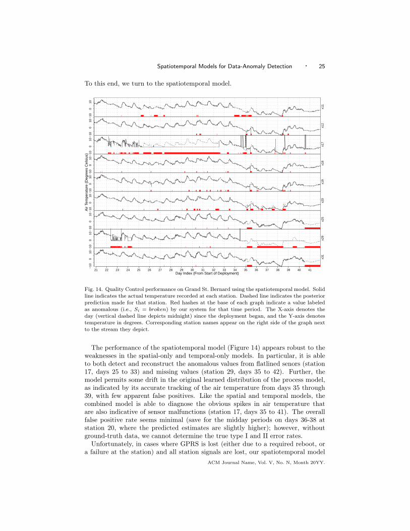
Spatiotemporal Models for Data-Anomaly Detection · 25
To this end, we turn to the spatiotemporal model.−
100
10
data[range, 2]
| ||||||||||||||||||||||||||||||||||| | |||||||||||||||||||||||||||||||||||||||||| ||||||||||||| ||| ||| ||||||||||||||||||||||||||||||||||||||||||||||||||||||||||||||||| ||||||||||||||||||||||||||||||||||||||||||||||||| ||||||| |||||||||||||||||||||||||||||||||||||||||| || ||||||
x11
−10
010
data[range, 2]
|||||||| ||||||||||||||||| | ||||||||||||||||||| ||||||||||| |||||||||||||| ||||||||||||
x12
−10
010
data[range, 2]
||||||||||||||||||||||||| ||||||| | || ||||||||||||||||||||||||||| |||||||||||||||||| ||||||||||||| ||| |||||||||||||||||||||||||||||||||||||||||||||||||||||||||||||||||| ||||||||||||||||||||||||||||||||||||||||||||||||||||||||||||||||||||||||||||||||||||||||||||||||||||||||| ||||||||||||||||||||||||||||||||||||||||||||||||||||||||||||||||||||||||||||||||||||||||||||||||||||||||||||||| ||||||||||||||||||||||||||||||||||||||||||||||||||||||||||||||||||||||||||||||||||||||||||||||||||||||||||||||||||||||||||||||||||||||||||||||||||||||||||||||||||||||||||||||||||||||||||||||||||||||||||||||||||||||||||||||||||||||||||||||||||||||||||||||||||||||||||||||||||||||||||||||||||||||||||||||||||||||||||||||||||||||||||||||||||||||||||||||||||||||||||||||||||||||||||||||||||||||||||||||||||||||||||||||||||||||||||||||||||||||||||||||||||||||||||||||||||||||||||||||||||||||||||||||||||||||||||||||||||||||||||||||||||||||||||||||||||||||||||||||||||||||||||||||||||||||||||||||||||||||||||||||||||||||||||||||||||||||||||||||||||||||||||||||||||||||||||||||||||||||||||||||||||||||||||||||||||||||||||||||||||||||||||||||||||||||||||| |||||||||||||||||||||||| | || ||||||||||||||||||||||||||||||||||||||||||||| ||||||||||||||||| || | | ||||| ||||| |||| |||||||
x17
−10
010
data[range, 2]
| | |||| |||| |||||| ||||| | |||| | |||||||| ||||||||||||||||||| | |||||| ||||
x18
−10
010
data[range, 2]
| ||||||| | |||||||||| |||||| ||||||||||||||||| ||||||| ||||||||| |||| | |||||||| || ||||||||||||||| ||||||||||||||||||||| |||||| || | |||| |||||| ||||| | |||||
x19
−10
010
data[range, 2]
|||| || ||||||||| | ||||||||||||| |||||||||||||||||||| |||||||||| ||||||||||| | ||||||||||||||||||||||||||||||||||||||||||| ||||||||||||| ||||||||||||||||||||| ||||||||||||||||||||||||||||||||||| | |||||||||||||||||||| |||||||||||||||||||||||||||||||||||| | ||||||||||||||||||||||||||||||||||||||
x20
−10
010
data[range, 2]
| | || || || || ||||||||||||||||||||||||||||||||||||||||||||||||||||||||||||||||||| ||||||||||||||||||||||||||||||||||||||||||||||||||||||||||||||||||||||||||||||||||||||||||||||||||||||||||||||||||||||||||||||||||||||||||||||||||||||||||||||||||||||||||||||||||||||||||||||||||||||||||||||||
x25
−10
010
data[range, 2]
||||||||||||||||||||||||||||||||||||||||||||||||||||||||||||||||||||||||||||||||||||||||||||||||||||||||||||||||||||||||||||||||||||||| |||||||| | |||||||||||||||||||||||||||||||||||||||||||||||||||| | ||| | ||||| | ||||||||||||||||||||||||||||||||||||||||||||||||||||||||||||||||||||||| ||||||||||||||||||||||||||||||||||||||||||||||||||||||||||||||||||||||||||||||||||||||||||||||||||||||||||||||||||||||||||||||||||||||||||||||||||||||||||||||||||||||||||||||||||||||||||||||||||||||||||||||||||||||||||||||||||||||||||||||||||||||||||||||||||||||||||||||||||||||||||||||||||||||||||||||||||||||||||||||||||||||||||||||||||||||||||||| ||||||||||||||||||||||||||||||||||||||||||||||||||||| ||||||||||||||||||||||||||||||||||||||||||||||||||||||||||||||||||||||||||||||||||||||||||||||||||||||||||||||||||||||||||||||||||||||||||||||||||||||||||||||||||||||||||||||||||||||||||||||||||||||||||||||||
x29
−10
010
data[range, 2]
| || | |||||||||||||||||||||||||||||||||||||||||||||||||||||||||||||||||| ||||||||||||||||||||||||||||||||||||||||||||||||||||||||||||||||||||||||||||||||||||||||||||||||||||||||||||||||||||||||||||||||||||||||||||||||||||||||||||||||||||||||||||||||||||||||||||||||||||||||||||||||
x31
21 22 23 24 25 26 27 28 29 30 31 32 33 34 35 36 37 38 39 40 41
Air
Tem
pera
ture
(D
egre
es C
elsi
us)
Day Index (From Start of Deployment)
Fig. 14. Quality Control performance on Grand St. Bernard using the spatiotemporal model. Solidline indicates the actual temperature recorded at each station. Dashed line indicates the posteriorprediction made for that station. Red hashes at the base of each graph indicate a value labeledas anomalous (i.e., Si = broken) by our system for that time period. The X-axis denotes theday (vertical dashed line depicts midnight) since the deployment began, and the Y-axis denotestemperature in degrees. Corresponding station names appear on the right side of the graph nextto the stream they depict.
The performance of the spatiotemporal model (Figure 14) appears robust to theweaknesses in the spatial-only and temporal-only models. In particular, it is ableto both detect and reconstruct the anomalous values from flatlined senors (station17, days 25 to 33) and missing values (station 29, days 35 to 42). Further, themodel permits some drift in the original learned distribution of the process model,as indicated by its accurate tracking of the air temperature from days 35 through39, with few apparent false positives. Like the spatial and temporal models, thecombined model is able to diagnose the obvious spikes in air temperature thatare also indicative of sensor malfunctions (station 17, days 35 to 41). The overallfalse positive rate seems minimal (save for the midday periods on days 36-38 atstation 20, where the predicted estimates are slightly higher); however, withoutground-truth data, we cannot determine the true type I and II error rates.
Unfortunately, in cases where GPRS is lost (either due to a required reboot, ora failure at the station) and all station signals are lost, our spatiotemporal model
ACM Journal Name, Vol. V, No. N, Month 20YY.

26 · E. Dereszynski and T. Dietterich
515
25
data[range, 2]
|||||||||||||||||||||||||||||||||||||||||||||||||||||||||||||||||||||||||||||||||||||||||||||||||||||||||||||||||||||||||||||||||| | | | |||||||||||||||||||||||||||||||||||||||||||||||||||||||||||||||||||||||||||||||||||||||||||||||||||||||||| ||||||||||||||||||||||||||||||||||||||||||||||||||||||||||||||||||||||||||||||||||||||||||||||||||||||||||||||||||||||||||||||||||||||||||||||||||||||||||||| |||||||||||||||||||||||||||||||||||||| |||||||||||||||||||||||||||||||||||||||||||||||||||||||| || |||||||||| ||||||||||||||||||||||||||||||||| ||||||||||||||||||||||||||||||||||||||||||||||||||||||| ||||||||||||||||||||||||||||||||| ||||||||||| | || ||| | |||||||||||||||||||||||||| |||||||||||||||||||||||||||||||||||||||||||||||||||||||||
x101
515
25
data[range, 2]
|||||||||||||||||||||||||||||||||||||||||||||||||||||||||||||||||||||||||||||||||||||||||||||||||||||||||||||||||||||||||||||||||| | |||||||||||||||||||||||||||||||||||||||||||||||||||||||||||||||||||||||||||||||||||||||||||||||||||||||||| ||||||||||||||||||||||||||||||||||||||||||||||||||||||||||||||||||||||||||||||||||||||||||||||||||||||||||||||||||||||||||||||||||||||||||||||||||||||||||||| ||||||||||||||||||||||||||||||||||||| ||||||||||||||||||||||||||||||||||||||||||||||||||||||||| |||||||||||| |||||||||||||||||||||||||||||||||||||||||||||| ||||||| |||||||||||||||||| |||||| | ||||||||||||||||||||||||| |||||||||||||||||||||||||||||||||||||||||||||||||||||||
x102
515
25
data[range, 2]
| |||||||||||||||||||||||||||||||||||||||||||||||||||||||||||||||||||||||||||||||||||||||||||||||||||||||||||||||||||||||||||| ||||||||||||||||||||||||||||||||||||||||||||||||||||||||||||||||||||||||||||||||||||||||||||||||||||||||||| |||||||||||||||||||||||||||||||||||||||||||||||||||||||||||||||||||||||||||||||||||||||||||||||||||||||||||||||||||||||||||||||||||||||||||||||||||||||||||| ||||| ||||||| |||||||||||||||||||||||||||||||||||||| ||||||||||||||||||||||||||||||||||||||||||||||||||||||||| | ||||||||||||||||||||||||||||||||||||||| ||||||||||||||||||||||||||||||||||||||||||||||||||||||| | ||||||||||||||||||||||||| ||| ||| | ||||||| ||| |||||||||||| ||||| ||||| || | ||||||||||||||||||||||||| |||||||||||||||||||||||||||||||||||||||||||||||||||||||
x103
515
25
data[range, 2]
| ||||||||||||||||||||||||||||||||||||||||||||||||||||||||||||||||||||||||||||||||||||||||||||||||||||||||||||||||||||||||||||||||||| || |||||||||||||||| ||||||||||||||||||||||||||||||||||||||||||||||||||||||||||||||||||||||||||||||||||||||||||||||||||||||||||| |||||||||||||||||||||||||||||||||||||||||||||||||||||||||||||||||||||||||||||||||||||||||||||||||||||||||||||||||||||||||||||||||||||||||||||||||||||||||||| |||||||||||||| |||||||||||||||||||||||||||||||||||||||||||| |||||||||||||||||||||||||||||||||||||||||||||||||||||||||||||||||||||||||||||||||||||||||||||||||||| |||||||| |||||||||||||||||||||||||| |||||||||||||||||||||||||||||||||||||||||||||||||||||||||||||||
x104
515
25
data[range, 2]
| |||||||||||||||||||||||||||||||||||||||||||||||||||||||||||||||||||||||||||||||||||||||||||||||||||||||||||||||||||||||||||| ||||||||||||||||||||||||||||||||||||||||||||||||||||||||||||||||||||||||||||||||||||||||||||||||||||||||||| |||||||||||||||||||||||||||||||||||||||||||||||||||||||||||||||||||||||||||||||||||||||||||||||||||||||||||||||||||||||||||||||||||||||||||||||||||||||||||||| ||| |||||||||||||||||||||||||||||||||||||| |||||||||||||||||||||||||||||||||||||||||||||||||||||||||||||||||||||||||||||||||||||||||||||||||||| |||||||| ||||||||||||||||||||||||| |||||||||||||||||||||||||||||||||||||||||||||||||||||||||||||||
x105
515
25
data[range, 2]
| |||||||||||||||||||||||||||||||||||||||||||||||||||||||||||||||||||||||||||||||||||||||||||||||||||||||||||||||||||||||||||||| ||||||||||||||||||||||||||||||||||||||||||||||||||||||||||||||||||||||||||||||||||||||||||||||||||||||||||| ||||||||||||||||||||||||||||||||||||||||||||||||||||||||||||||||||||||||||||||||||||||||||||||||||||||||||||||||||||||||||||||||||||||||||||||||||||||||||||||| || | |||| |||||||||||||||||||||||||||||||||||||| |||||||||||||||||||||||||||||||||||||||||||||||||||||||||||||||||||||||||||||||||||||||||||||||||||| |||||||| | |||||||||||||||||||||||||| ||||||||||||||||||||||||||||||||||||||||||||||||||||||||||||||||
x106
15 16 17 18 19 20 21 22 23 24 25 26 27
Air
Tem
pera
ture
(D
egre
es C
elsi
us)
Day Index (From Start of Deployment)
Fig. 15. Quality Control performance on FishNet using the spatiotemporal model. Solid lineindicates the actual temperature recorded at each station. Dashed line indicates the posteriorprediction made for that station. Red hashes at the base of each graph indicate a value labeledas anomalous (i.e., Si = broken by our system for that time period. The X-axis denotes theday (vertical dashed line depicts midnight) since the deployment began, and the Y-axis denotestemperature in degrees. Corresponding station names appear on the right side of the graph nextto the stream they depict.
cannot recreate the missing values. This is apparent in the FishNet dataset, whereGPRS outages were relatively frequent (Figure 15) compared to Grand St. Bernard.In cases where no sensors are providing observations, the variance over the jointposterior of the current process state grows. This is because a lack of evidenceabout the state of the process means that we are becoming increasingly uncertainabout its current value. Eventually, the variance will grow so large that almost anyobserved value will seem likely, and so our process will begin to retrack the observa-tions. When the sensor readings resume, the very first observation is recognized asnonanomalous and causes the spatial and temporal components to shift the processmodel to that observed value for all correlated sensors. For example, during theoutage beginning on day 18.5 and lasting until day 19.75, there is a single obser-vation around day 19.5 that causes the collective temperature prediction for moststations to shift down 4 ℃. Otherwise, during these periods of prolonged GPRSoutage, the prediction will drift toward the mean for each station while variance onthe prediction grows larger.
Without knowledge of neighboring observations within a site or a sufficientlyACM Journal Name, Vol. V, No. N, Month 20YY.

Spatiotemporal Models for Data-Anomaly Detection · 27
high-order Markovian model, there is little the current model can do to correctlytrack the air temperature during periods in which all sensors fail to report. Onepotential solution would be to introduce a baseline calculation that represents priorknowledge about the air temperature at a given site for each time of day andtime of year. In the absence of evidence to correct this baseline estimate, themodel would default to the baseline values. While the baseline may be inaccurategiven the temporal context (warmer/cooler than usual, storm effect, etc.), it wouldlikely guide the process model such that it was closer to the actual signal whenobservations recommenced. Formulation of this baseline and its performance in along-term stationary QC domain is reported in Dereszynski and Dietterich [2007].The problem remains that, in the short-term ecological monitoring setting, it maybe difficult to estimate this baseline in the absence of a full cycle of the observedphenomenon (one year in the case of air temperature).
6.3 Noise Injection Experiments
To obtain a quantitative assessment of the accuracy of our quality control methods,we performed a series of experiments in which we injected noise into the SensorScopedata. Initially, all readings are assigned to be nonanomalous. Then any missingvalues or 10-minute average of exactly -1.0 degrees ℃ are labeled as anomalous.Finally, synthetic faults are introduced by taking each data point and, with prob-ability η, adding a noise value drawn from a normal distribution with zero meanand variance σ2
n. Each synthetic fault is labeled as anomalous.We report the results of the noise injection experiments for both the FishNet and
Grand St. Bernard deployments. The experiments were performed using valuesof σ2
n ranging from 3 ℃ to 30 ℃ in increments of 3 ℃ and values of η rangingfrom 5 to 50 percent in increments of 5 percent. Thus, we evaluate 100 differentvariations on the testing data for each dataset, and record the results in terms ofthe number of true positives (TP , number of anomalous data values classified byour system as such), true negatives (TN , the amount of clean values that werenot flagged by our system as anomalous), false positives (FP , misclassified anoma-lies that were actually clean), and false negatives (FN , values that were actuallyanomalous, but not detected by our system). The results are summarized in termsof Cohen’s κ statistic (the rate of agreement between our classifier and the truelabels correcting for chance agreement [Cohen 1960]), precision (the total numberof true positives divided by the number of true positives plus false positives), andrecall (the total number of true positives divided by the number of true positivesplus false negatives). Cohen’s κ reflects the degree to which our algorithm repro-duces the true labels as created by our noise injection process corrected for chancepredictions [Cohen 1960; Viera and Garrett 2005]. It is calculated as
κ =P (O)− P (E)
1.0− P (E), (25)
P (O) =TP + TN
FN, (26)
P (E) =TN + FP
N× TN + FN
N+FP + TP
N× FN + TP
N, (27)
where P (O) is the observed probability of the classifier agreeing with the true label,ACM Journal Name, Vol. V, No. N, Month 20YY.

28 · E. Dereszynski and T. Dietterich
P (E) is the expected probability of chance or coincidental agreement, and N is thetotal number of samples in our testing data. Regarding the latter two statistics,precision provides a sense of how many of the values we label as anomalous aretruly indicative of sensor faults, while recall summarizes what percent of the totalgenuine sensor faults we detect in the data. In this application, we are interestedin achieving as much precision as possible at high levels of recall. In other words,we want to make sure we detect most of the sensor faults, even if this leads to somefalse alarms (false positives).
Let us consider what results we should expect from injecting noise. First, wewould expect that as the magnitude of the noise (σ2
n) increases, the noise willbecome easier to detect, because it will be clearly distinct from nearby values intime and space. Increasing the amount (η) of noise should not decrease our abilityto detect it; however, fewer non-noisy values will make tracking short-term changesin the air temperature (due to storm effects, cold/warm fronts, etc.) more difficult.For this reason, we expect that larger values η will result in more false positives incases where the model loses tracking and its predictions drift away from the trueair temperature. Ultimately, the best data-anomaly detection performance will beobtained when there is a small amount of very obvious noise in the data (small ηand large σ2
n).
% Noise Injected
Var
ianc
e (D
egre
es C
elsi
us)
FishNet Kappa
5 10 15 20 25 30 35 40 45 50
3
6
9
12
15
18
21
24
27
30
0
0.1
0.2
0.3
0.4
0.5
0.6
0.7
0.8
0.9
1Grand St. Bernard Kappa
% Noise Injected
Var
ianc
e (D
egre
es C
elsi
us)
5 10 15 20 25 30 35 40 45 50
3
6
9
12
15
18
21
24
27
30
0
0.1
0.2
0.3
0.4
0.5
0.6
0.7
0.8
0.9
1
Fig. 16. κ as a function of both noise variance (Y-axis) and percentage of data points modifiedby noise (X-axis). The shade of color associated with each grid cell reflects the degree of κ (on ascale of 0 to 1.0) for that configuration of noise level and saturation.
Figure 16 shows the κ rates of our model applied to the FishNet (left) and GrandSt. Bernard (right) deployments. The value of κ is displayed on a color scale, withhigher values shown in darker shades of red and lower values shown in darker shadesof blue. As expected, larger values of σ2
n resulted in better κ scores for both theFishNet and Grand St. Bernard data sets. Data anomalies drawn from a highervariance distribution are more evident to our classifier; consequently, there is moregenuine agreement. In the of case FishNet, κ increases from .527 to .826 as weincrease σ2
n from 3 to 30, and from .440 to .755 in the case of Grand St. Bernard(at η = 20%). Interesting to note is that more noise in the data does not have anadverse effect on our κ scores until more than 25% to 30% noise is introduced. Infact, the κ scores for both data sets increase up to this point. As more anomalies areACM Journal Name, Vol. V, No. N, Month 20YY.

Spatiotemporal Models for Data-Anomaly Detection · 29
introduced into the data and correctly identified by our algorithm, the likelihood ofcoincidental agreement (P (E)) decreases; however, there appears to be a thresholdat approximately 25% noise where κ begins to decrease. This suggests a tradeoffwhere further abundance of anomalies in the data makes them appear haphazardrather than systematic.
FishNet Precision
% Noise Injected
Var
ianc
e (D
egre
es C
elsi
us)
5 10 15 20 25 30 35 40 45 50
3
6
9
12
15
18
21
24
27
30
0
0.1
0.2
0.3
0.4
0.5
0.6
0.7
0.8
0.9
1Grand St. Bernard Precision
% Noise Injected
Var
ianc
e (D
egre
es C
elsi
us)
5 10 15 20 25 30 35 40 45 50
3
6
9
12
15
18
21
24
27
30
0
0.1
0.2
0.3
0.4
0.5
0.6
0.7
0.8
0.9
1
Fig. 17. Precision as a function of both noise variance (Y-axis) and percentage of data pointsmodified by noise (X-axis). The shade of color associated with each grid cell reflects the degreeof precision (on a scale of 0% to 100%) for that configuration of noise level and saturation.
Precision results in Figure 17 further support our hypothesis regarding the effectof larger values for σ2
n. The true anomalies are more disparate from the normal data,and so the ratio of true positives to false positives increases directly with magnitudeof the noise (fewer false positives result in higher precision scores). Further, as weincrease the amount of noise in the data, any value we classify as anomalous has ahigher chance of actually being so due to a greater proportion of the data containingnoise. When there are few anomalies in the data (5% injected noise), our scoressuffer due to the presence of relatively many false positives. Consider our falsepositive rates (percent of all “good” data missclassified as anomalous) shown inFigure 18. Though we achieve very low false positive rates at this level of noise(average of 1.01% at FishNet and 3.08% at Grand St. Bernard for η = 5%), thereare too few synthetic anomalies in the data, causing the false positive counts todominate the precision scores. In addition, while some of these false positives are“good” values misdiagnosed as anomalies by our system, it is likely that manyof these errors come from suspicious values that we did not pre-flag as existinganomalies due to a lack of domain expertise (for example, sensors 17 and 29 ofGrand St. Bernard on days 22 through 25 in Figure 12). Thus, even though ourmodel is catching these likely faults, each is being labeled as a false positive.
There are cases where poor performance is caused by multiple sensor streamsbeing affected by noisy values simultaneously. Consider the QC model appliedto the noise-injected data in Figure 19 (η = 50, σ2
n = 15). Beginning on day36, a cooling trend affects all stations in the deployment and reduces the true airtemperature below 0 degrees ℃. Incidentally, station 29 flatlines at exactly -1.0degrees ℃ during this period. As the true signal dips below -1.0 degrees ℃, wenotice that all stations begin predicting values hovering near this boundary until
ACM Journal Name, Vol. V, No. N, Month 20YY.

30 · E. Dereszynski and T. Dietterich
FishNet False Positive Rate
% Noise Injected
Var
ianc
e (D
egre
es C
elsi
us)
5 10 15 20 25 30 35 40 45 50
3
6
9
12
15
18
21
24
27
30
0
0.05
0.1
0.15
0.2
0.25
0.3
0.35
0.4
0.45
0.5Grand St. Bernard False Positive Rate
% Noise Injected
Var
ianc
e (D
egre
es C
elsi
us)
5 10 15 20 25 30 35 40 45 50
3
6
9
12
15
18
21
24
27
30
0
0.05
0.1
0.15
0.2
0.25
0.3
0.35
0.4
0.45
0.5
Fig. 18. False Positive rates as a function of both noise variance (Y-axis) and percentage of datapoints modified by noise (X-axis). The shade of color associated with each grid cell reflects thedegree of precision (on a scale of 0% to 50%) for that configuration of noise level and saturation.
the cooling trend ends around day 39. Further, instead of recognizing the valuesreported from station 29 as anomalous for this period (as in Figure 14), these valuesare the only ones labeled as nominal. This behavior occurs because the amount anddegree of injected noised in the data makes it unlikely that a set of observations attime t will be consistent with the spatial component of the QC model, and makes iteven less likely that two sets of contiguous observations (times t and t+ 1) will beconsistent with the temporal transition component. During this period, station 29behaves very consistently from a temporal perspective (its observations are constantfrom day 34.5 to 40.5), and the variance of the injected noise is enough to bringthe observed signal from the other stations within close proximity of the flatlinevalue. The end result is that station 29 becomes the standard for nominal behavioruntil the true temperature deviates from the flatline by a margin larger than themagnitude of added noise.
In the above-mentioned scenario, increased values of both η and σ2n negatively
affect the precision score. As η increases, the likelihood of all sensors encoun-tering noisy values simultaneously also rises. Noisy observations drawn from awide-variance distribution are more likely to strongly disagree with the QC model’spredictions and, as a result, this frequently causes the model to ignore such ob-servations. This kind of scenario becomes more probable in cases where there arerelatively few, highly-correlated sensors that are prone to simultaneous malfunc-tioning.
Recall values, displayed in Figure 20, are largely invariant to changing values ofη. Increasing the amount of noise in the original data has no significant effect onour ability to find all data anomalies. This is unsurprising. As per our discussionof precision, an abundance of anomalous values may introduce tracking problemsthat leads to misclassifying normal values as anomalous; however, false positivevalues do not factor into recall scores. An increase in the magnitude of the noisedistribution directly benefits our recall scores, which is again consistent with ourhypothesis. In both data sets, we are able to achieve greater than .70 recall oncethe variance of the noisy data reaches 15 ℃. For the FishNet deployment, we cansimultaneously reach a precision score of .87 while keeping our false positive rateACM Journal Name, Vol. V, No. N, Month 20YY.

Spatiotemporal Models for Data-Anomaly Detection · 31
−10
010
data[range, 2]
||||||||||||||||||||||||||||||||||||||||||||||||||||||||||||||||||||||||||||||||||||||||||||||||||||||||||||||||||||||||||||||||| |||||||||||||||||||||||||||||||||||||||||||||||||||||||||||||||||||||||||||||||||||||||| | ||||||||||||||||||||||||||||||||||||||||||||||||||||||||||||||||||||||||| |||||||||||||||||||||||||||||||||||||||||||||||||||||||||||||||||||||||||||||||||||| | |||||||||||||||||||||||||||||||||||||||||||||||||||||||||||||||||||||||||||||||||||||||||||||||||||||||||||||||||||||||||||||||||||| ||| |||||||||| ||| |||||||||| |||||||||||||||||||||||||||||||||||||||||||||||||||||||||||||||||||||||||||||||||||||||||||||||||||||||||||||||||||||||||||||||||| |||||||||||||||||||||||||||||| |||||| |||||||||||||||||||||||||||||||||||||||||||||||||||||||||||||||||||||||||||||||||||||||||||| ||||||||||||||||||||||||||||||||||||||||||||||||||||||||||||||||||||||||||||||||||||||||||||||||||||||||||||||||||||||||||||||||||||||||||||||||||||||||||||||||||||||||||||||||||||||||||||||||||||||||||||||||||||||||||||||||||||||||||||||||||||||||||||||||||||||||||||||||||||||||||||||||||||||||||||||||||||||||||||||||||||||||||||||||||||||||||||||||||||||||||||||||||||||||||||||||||||||||||||||||||||||||||||||||||||||||||||||||||||||||||||||||||||||||||||||||||||||||||||||||||||||||||||||||||||||||||||||||||||||||||||||||||| |||||||||||| ||||||| ||||||||||||||||| |||||||||||||||||||||||||||||||||||||||||||||||||||||||||||||||||||||||||||||||||||||||||||||||||||||||| |||||||||||||||||||||||||||||
x11
−10
010
data[range, 2]
||||||||| |||||||||||||||||||||||||||||||||||||||||||||||||||||||||||||||||||||||||||||||||||||||||||||||||| |||||||||||||||||||||||||||||||||||||||||||||||||| | ||||||||||||||||||||||||||||||||||||||||||||||||||||||||||||||||||||||||||||||||||||||||||||||||||||||||||||||||||||||||||||||||||||||| |||||||||||||||||||||||||||||||||||||||||||||| ||||||||||||||||||||||||||| ||||||||||||||||||||||||||||||||||||||||||||||||||||||||||||||||||||||||||||||||||||| ||||||||||||||||||||||||||||||||||||||||||||||||||||||||||||||||||||||||||||||||||||||||||||||||||||||||||||||||||||||||||||||||||||||||||||||||||||||||||||| |||||||||||||||||||||||||||||||||||||||||||||||||||||||||||||||||||||||||||||||||||||||||||||||||||||||||||||||||||||||||||||||||||||||||||||||||||||||||||||||||||||||||||||||||||||||||||||||||||||||||||||||||||||||||||||||||||||||||||||||||||||||||||||||||||||||||||||||||||||||||||||||||||||||||||||||||||||||||||||||||||||||||||||||||||||||||||||||||||||||||||||||||||||||||||||||||||||||||||||||||||||||||||||||||||||||||||||||||||||||||||||||||||||||||||||||||||||||||||||||||||||||||||||||||||||||||||||||||||||||||||||||||||||||||||||||||||||||||||||||||||||||||||||||||||||||||||||||||||||||||||||||||||||||||||||||||||||||||||||||||||||||||||| |||||||||||||||||||||||||||||||||||||||||||||||||||||||||||||||||||||||||||||||||||||||||||||||||||||||||||||||||||||||||||||||| |||||||||||||||||||| ||||||||||||||||||||||||||||||||||||
x12
−10
010
data[range, 2]
||||||||||||||||||||||||||||||||||| ||||||||||||||||||| |||||||||||||||||||||||||||||||||||||||| ||||||||||||||||||||||||||||||||||||||||||||||||||||||||||||||||||||||||||||||||||||||||||||||||| ||||||||||||||||||||||||||||||||||||||||||||||||||||||||||||||||||||||||||||||||||||||||||||||||||||||||||||||||||| ||||||||||||||||||||||||||||||||||||||||||||||||||||||||||||||||||||||||||||||||||||||||||||||||||||||| ||||||||||||||||||||||||||||||||||||||||||||||||||||||||||||||||||||||||||||||||||||||||||||||||||||||||||||||||||||||||||| |||| |||||||||||||||||||||||||||||||||||||||||||||||||||||||||||||||||||||||||||||||||||||||||||||||||||||||||||||||||||||||||||||||||||||||||||||||||||||||||||||||||||||||||||||||||||||||||||||||||||||||||||||||||||||||||||||||||||||||||||||||||||||||||||||||||||||||||||||||||||||||||||||||||||||||||||||||||||||||||||||||||||||||||||||||||||||||||||||||||||||||||||||||||||||||||||||||||||||||||||||||||||||||||||||||||||||||||||||||||||||||||||||||||||||||||||||||||||||||||||||||||||||||||||||||||||||||||||||||||||||||||||||||||||||||||||||||||||||||||||||||||||||||||||||||||||||||||||||||||||||||||||||||||||||||||||||||||||||||||||||||||||||||||||||||||||||||||||||||||||||||||||||||||||||||||||||||||||||||||||||||||||||||||||||||||||||||||||||||||||||||||||||||||||||||||||||||||||||||||||||||||||||||||||||||||||||||||||||||||||||||||||||||||||||||||||| || ||||||||||||||||||||||||||||||||||||||||||||||||||||||||||||||||||||||||||||||||||||||||||||||||||||||||||||||||||||||||||||||||||||||||||||||||||||||||||||||||||||||||||||||||||||||||||||||||||||||||||||||||||||||||||||||||||||||||||||||||||||||||||||||||||||||||||||||||||||||||||||||||||||||||||||||||||||||||||||||||||||||||||||||||||||||||||||||||||||||||||||||||||||||||||||||||||||||||||||||||||||||||||||||||||||||||||||||||||||||||||||||||||||||||||||||||||||||||||||||||||||||||||||||||||||||||||||||||||||||||||||||| ||||||||||||||||||||||||||||||||||||||||||||||||||||||||||||||||||||||||||||||||||||||||||||||||||||||||||||||||||||||||||||||||||||||||||| ||||||||
x17
−10
010
data[range, 2]
||||||||||||||||||||||||||||||||||||||||| ||||||||||||||||||||||||||| |||||||||||||||||||| |||| ||||||||||||||||||||||||||||||||||||||||||||||||||||||||||||||||||||||||||||||||||||||||||||||||||||||||||| ||||||||||||||||||||||||||||||||||||||||||||||| |||||||||||||||||||||||||||||||||||||||||||||||||||||||||||||||||||||||||||||||||||||||||||||||||||||||||||||||| |||||||||||||||||||||||||||||||||||||||||||||||||||||||||||||||||||||||||||||| |||||||||||||||||||||||||||||||||||||||||||||||||||||||||||||||||||||||||||||||||||||||||||||| |||||||||||||||||||||| ||||||||||||||||||||||||||||||||||||||||||||||||||||||||||||||||||||||||||||||||||||||||||||||||||||||||||||||||||||||||||||||| ||||||||||||||||||||||||||||||||||||||||||||||||||||||||||||||||||||||||||||||||||||||||||||||||||||||||||||||||||||||||||||||||||||||||||||||||||||||||||||||||||||||||||||||||||||||||||||||||||||||||||||||||||||||||||||||||||||||||||||||||||||||||||||||||||||||||||||||||||||||||||||||||||||||||||||||||||||||||||||||||||||||||||||||||||||||||||||||||||||||||||||||||||||||||||||||||||||||||||||||||||||||||||||||||||||||||||||||||||||||||||||||||||||||||||||||||||||||||||||||||||||||||||||||||||||||||||||||||||||||||||||||||||||||||||||||||||||||||||||||||||||||||||||||||||||||||||||||||||||||||||||||||||||||||||||||||||||||||||||||||||||||||||||||||||||||||||||||||||||||||||||||||||||||||||||||||||||||||||||||||||||||||||||||||||||||||||||
x18
−10
010
data[range, 2]
||||||||||||||||||||||||||||||||||||||||||||||||||||||||||||||||||||||||||||||||||||||||||||||||||||||||||||||||||||||||||||| |||||||||||||||||||||||||||||||| ||||||||||||||||||||||||||||||||||||||||||||||||||||||||||||||||||||||||||||||||||||||||||||||||||||||||||||||||||||||||||||||||||||||||||||||||||||||||||||||||||| |||||||||||||||||||||||||||||||||||||||||||||||||||||||||||||||||||||||||||||||||||||||||||||||||||||||||||||||||||||||||||||||||| ||||||||||||||||||||||||||||||||||||||||||||||||||||||||||||||||||||||||||||||||||||||||||||||||||||||||||||||||||||||||||||||||||||||||||||||||||||||||||||||||||||||||||||||||||||||||||||||||||||||||||||||| ||| ||||||||||||||||||||||||||||||||||||||||||||||||||||||||||||||||||||||||||||||||||||||||||||||||||||||||||||||||||||||||||||||||||||||||| |||||||||||||||||||||| ||||||||||||||||||||||||||||||||||||||||||||||||||||||||||||||||||||||||||||||||||||||||||||||||||||||||||||||||||||||||||||||||||||||||||||||||||||||||||||||||||||||||||||||||||||||||||||||||||||||||||||||||||||||||||||||||||||||||||||||||||||||||||||||||||||||||||||||||||||||||||||||||||||||||||||||||||||||||||||||||||||||||||||||||||||||||||||||||||||||||||||||||||||||||||||||||||||||||||||||||||||||||||||||||||||||||||||||||||||||||||||||||||||||||||||||||||||||||||||||||||||||||||||||||||||||||||||||||||||||||||||||||||||||||||||||||||||||||||||||||||||||||||||||||||||||||||||||||||||||||||||||||||||||||||||||||||||||||||||||||||||||||||||||||||||||||||||||||||||||||||||||||||||||||||||||||||||||||||||||||||||||||||||||||||||||||||||||||||||||
x19
−10
010
data[range, 2]
|||||||||| ||||||||||||||||||||||||||||||||||||||||||||||||||||||||||||||||||||||| ||||||||||||||||||| |||||||||||||||||||||||||||||||||||||||||||||||||||||||||||||||||||||||||||||||||||||| |||||||||||||||||||||||||||||||||||||||||||||||||||||||||||||||| |||||||||||||||||| ||||| ||||||||||||| ||||||||||||||||||||||||||||||||| |||||||| |||||||||||||||||||||||||||||| |||||||||||||||||||||||||||||||||||||||||||||||||||||||||||||||||||||||||||||||||||||||||||||||||||||||||||||||||||||| |||||||||||||||||||||||||||||||||||||||||||||||||||||||||||||||||||||||||||||||||||||||||||||||||||||||||||||||||||||||||||||||||||||||||||||||||||||||||||||||||||||||||||||||||||||||||||||||||||||||||||||||||||||||||||||||||||||||||||||||||||||||||||||||||||||||||||||||||||||||||||||||||||||||||||||||||||||||||||||||||||||||||||||||||||||||||||||||||||||||||||||||||||||||||||||||||||||||||||||||||||||||||||||||||||||||||||||||||||||||||||||||||||||||||||||||||||||||||||||||||||||||||||||||||||||||||||||||||||||||||||||||||||||||||||||||||||||||||||||||||||||||||||||||||||||||||||||||||||||||||||||||||||||||||||||||||||||||||||||||||||||||||||||||||||||||||||||||||||||||||||||||||||||||||||||||||||||||||||||||||||||||||||||||||||||||||||||||||||||||||||||||||||||||||||||||||||||||||||||||||||||||||||||||||||||||||||||||||||||||||||||||||||||||||||||||||||||||||||||||||||||||||||||||||||||||||||||||||||||||||||||||||||||||||||||||||||||||||||||||||||||||||||||||||||||||||||||||||||||||||||||||||||||||||||||||||| |||||||||||||||||||||||||||||||||||||||||||||||||||||||
x20
−10
010
data[range, 2]
|||||||||||||||||||| ||||||||||||||||||||||||||||||||||||||||||||||||||||||||||||||||||||||||||||||||||||||||||||||||||||| ||||||||||||||||||||||||||||||||||||||||||||||||||||| ||||||||||||||||||||||||||||||||||||||||||||||||||||||||||||||||||||||||||||||||||||||||||| ||||||||||||||||||||||||||||||||||||||||||||||||||||||||||||||||||||||||||||||||||||||||||||||||||||||||||||||||||||||||||||||||||||||||||||||| ||||||||||||||||||||||||| ||||||||||||||||||||||||||||||||||||||||||||||||||||||||||||||||||||||||||||||||||||||||||||||||||||||||||||||||||||||||||||||||||||||| |||||||||||||||||||||||||||||||||||||||||||||||||||||||||||||||||||||||||||||||||||||||||||||||||||||||||||||||||||||||||||||||||||||||||||||||||||||||||||||||||||||||||||||||||||||||||||||||||||||||||||||||||||||||||||||||||||||||||||||||||||||||||||||||||||||||||||||||||||||||||||||||||||||||||||||||||||||||||||||||||||||||||||||||||||||||||||||||||||||||||||||||||||||||||||||||||||||||||||||||||||||||||||||||||||||||||||||||||||||||||||||||||||||||||||||||||||||||||||||||||||||||||||||||||||||||||||||||||||||||||||||||||||||||||||||||||||||||||||||||||||||||||||||||||||||||||||||||||||||||||||||||||||||||||||||||||||||||||||||||||||||||||||| |||||||||||||||||||||| ||||||||||||||||||||||||||||||||||||||||||||||||||||||||||||||||||||||||||||||||||||||||||||||||||||||||||||||||||||||||||||||||||||||||||||||||||||||||||||||||||||||||||||||||||||||||||||||||||||||||||||||||||||||||
x25
−10
010
data[range, 2]
||||||||||||||||||||||||||||||||||||||||||||||||||||||||||||||| ||||||||||||||||||||||||||||||||||||||||||||||||||||||||||||||||||||||||||||||||||||||||||||||||||||||||||||||||||||||||||||||||||||||||||||||||||||||||||||||||||||||||||||||||||||||||||||||||||||||||||||||||||||||||||||||||||||||||||||||||||||||||||||||||||||||||||||||||||||||||||||||||||||||||||||||||||||||||||||||||||||||||||||| |||||||||||||||||||||||||||||||||||||||||||||||| |||||||||||||| |||||||||||||||||||| |||| |||||||||||||||||||||||||||||||||||||||||||||||||||||||||||||||||||| ||||||||||||||||||||||||||||||||||||||||||||||||||||||||||||||| ||||||||||||||||||||||||||||||||||||||||||||||||||||||||||||||||||||||||||||||||||||||||||||||||||||||||||||||||||||||||||||||||||||||| |||||||||| |||||||||| | ||||||||||||||||||||||||||||||||||||||||||||||||||||||||||||||||||||||||||||||||| |||||| |||||||||||||||||||||||||||||||||||||||| ||||||||||||||||||||||||||||||||||||||||||||||||||||||||||||||||||||||||||||||||||||||||||||||||||||||||||||||||||||||||||||||||||||||||||||||||||||||||||||||||||||||||||||||||||||||||||||||||||||||||||||||||
x29
−10
010
data[range, 2]
||||||||||||||||||||||||||||||||||||||||||||||||||||||||| |||||||||||| |||||||||||||||||||||||||||||||||| |||||||||||||||||||||||||||||||||||||||||||||||||||||||||||||||||||| ||||||||||||||| ||||||||||||||||||||||||||||||||||||||||||||||||||||||||||||||||||||||| ||||||||||||||||||||||||||||||||||||||||||||||||||||||||||||||||||||||||||||||||||||||||||||||||||||||||||||||||||||||||||||||||||||||||||||||||||||||||||||||| |||||||||| ||||||| ||||||||||||||||||||||||||||||||||||||||||||||||||||||||||||||||||||||||||||||||||||||||||||||||||||||||||||||||||||||||||||| |||||||||||||||||||||||||||||||||||||||||||| |||||||||||||||||||||||||||||||||||||||||||| ||||||||||||||||||||||||||||| ||||||||||||||||||||||||||||||||||||||||||||||||||||||||||||||||||||||||||||||||||||||||||||||||||||||||||||||||||||||||||||||||||||||||||||||||||||||||||||||||||||||||||||||||||||||||||||||||||||||||||||||||||||||||||||||||||||||||||||||||||||||||||||||||||||||||||||||||||||||||||||||||||||||||||||||||||||||||||||||||||||||||||||||||| |||||||||||||||||||||||||||||||||||||||||||||||||||||||||||||||||||||||||||||||||||||||||||||||||||||||||||||||||| |||||||||||||||||||||||||| |||||||||||||||||||| ||||||||||||||||||||||||||||||||||||||||||||||||||||||||||||||||||||||||||||||||||||||||||||||||||||||||||||||||||||||||||||||||||||||||||||||||||||||||||||||||||||||||||||||||||||||||||||||||||||||||||||||||||||||||||||||||||||||||||||||||||||||||||
x31
21 22 23 24 25 26 27 28 29 30 31 32 33 34 35 36 37 38 39 40 41
Air
Tem
pera
ture
(D
egre
es C
elsi
us)
Day Index (From Start of Deployment)
Fig. 19. QC results for Grand St. Bernard data with 50% added Gaussian noise with variance of15 ℃. Red hash marks depict a sensor diagnosis of broken for that particular value. Correspondingstation names appear on the right side of the graph next to the stream they depict.
at 4.6%. At Grand St. Bernard, we operate at .78 precision with a false positiverate of 7.0%. Again, Grand St. Bernard’s worse performance is partially due tothe presence of suspicious values that we did not preflag as data anomalies beforeinjecting noise.
FishNet Recall
% Noise Injected
Var
ianc
e (D
egre
es C
elsi
us)
5 10 15 20 25 30 35 40 45 50
3
6
9
12
15
18
21
24
27
30
0
0.1
0.2
0.3
0.4
0.5
0.6
0.7
0.8
0.9
1Grand St. Bernard Recall
% Noise Injected
Var
ianc
e (D
egre
es C
elsi
us)
5 10 15 20 25 30 35 40 45 50
3
6
9
12
15
18
21
24
27
30
0
0.1
0.2
0.3
0.4
0.5
0.6
0.7
0.8
0.9
1
Fig. 20. Recall as a function of both noise variance (Y-axis) and percentage of data points modifiedby noise (X-axis). The shade of color associated with each grid cell reflects the degree of recall(on a scale of 0% to 100%) for that configuration of noise level and saturation.
ACM Journal Name, Vol. V, No. N, Month 20YY.

32 · E. Dereszynski and T. Dietterich
Lastly, we provide an individual analysis of the effects of increasing the frequencyand magnitude of noise in each of these datasets. Figure 21 shows the average κ,recall, and precision for the FishNet (left) and Grand St. Bernard (right) deploy-ments, as a function of only η (top) and only σ2
n (bottom). In the case of the topgraphs, each value on the vertical axis represents an averaging over all values forσ2n; likewise, each value on the vertical axis for the bottom graphs is an average
across all values for η.
0 10 20 30 40 50
0.2
0.6
1.0
Percent of Noise
Rat
e (%
)
●●●●●●●●●● ●●●●●●●●●● ●●●●●●●●●● ●●●●●●●●●● ●●●●●●●●●● ●●●●●●●●●● ●●●●●●●●●● ●●●●●●●●●● ●●●●●●●●●● ●●●●●●●●●●
●
KappaPrecisionRecall
0 5 10 15 20 25 30
0.2
0.6
1.0
Variance of Gaussian Noise (Degrees Celsius)
Rat
e (%
)
●●●●●●●●●●
●●●●●●●●●●●●●●●●●●●●
●●●●●●●●●● ●●●●●●●●●● ●●●●●●●●●● ●●●●●●●●●● ●●●●●●●●●● ●●●●●●●●●● ●●●●●●●●●●
●
KappaPrecisionRecall
FishNet
0 10 20 30 40 50
0.2
0.6
1.0
Percent of NoiseR
ate
(%)
●●●●●●●●●● ●●●●●●●●●● ●●●●●●●●●● ●●●●●●●●●● ●●●●●●●●●● ●●●●●●●●●● ●●●●●●●●●● ●●●●●●●●●● ●●●●●●●●●● ●●●●●●●●●●
●
KappaPrecisionRecall
0 5 10 15 20 25 30
0.2
0.6
1.0
Variance of Gaussian Noise (Degrees Celsius)
Rat
e (%
)
●●●●●●●●●●
●●●●●●●●●●●●●●●●●●●●
●●●●●●●●●●●●●●●●●●●● ●●●●●●●●●● ●●●●●●●●●● ●●●●●●●●●● ●●●●●●●●●● ●●●●●●●●●●
●
KappaPrecisionRecall
Grand St. Bernard
Fig. 21. Left: Precision, Recall, and κ for the FishNet noise injection experiments as function ofpercentage of noise (top) and degree of variance (bottom). Right: Precision, Recall, and κ for theGrand St. Bernard noise injection experiments as function of percentage of noise (top) and degreeof variance (bottom).
Increasing the amount (η) of anomalous values in the data resulted in a increase ofprecision for both data sets. The effect seems less pronounced for the FishNet dataset (.778 to .875) compared to Grand St. Bernard (.535 to .833) as η varies from 5%to 50%. Again, this is likely attributable to the existence of many suspicious valuesin the Grand St. Bernard dataset that were not preflagged as data anomalies. Priorto any Gaussian noise being added, these values would appear anomalous to ourmodel and would be classified as data anomalies. When η is small, it is unlikelyour noise injection process will target these observations and turn them into truecases of data anomalies. The end result is these observations become false positives.As η increases, more of these suspicious values are rightly cast as data anomaliesduring noise injection. κ increases initially with more noisy values injected into thedata; however, as discussed with the κ results, we see diminishing returns and aneventual loss in κ as η grows over 25% for both the FishNet and Grand St. Bernarddatasets.
The lower portion of Figure 21 shows a definite gain in overall precision, recall,and κ as the degree of noise in the data (σ2
n) rises from 3 ℃ to 30 ℃. Specifically, κincreases by approximately .3 in both data sets, recall increases by .34 in FishNetand .36 at Grand St. Bernard, and precision increases by .06 at FishNet and .08 atACM Journal Name, Vol. V, No. N, Month 20YY.

Spatiotemporal Models for Data-Anomaly Detection · 33
Grand St. Bernard. In regards to recall and κ, this is because as the added noise inthe data becomes more obvious (higher variance), it becomes easier for our modelto detect it. The increase in precision is less pronounced than the increase in recalland κ, which could be caused by our QC model having too a great a sensitivity toanomalous values (too small of a variance for the sensor observation variable whenthe sensor state is believed to be working).
6.4 Noise Injection & Model Comparison
In this section we use our noise injection methodology to validate that learninga spatial model provides superior performance than arbitrarily choosing a spatialstructure. We examine four spatiotemporal QC models.
—Best : QC model having the highest-scoring (best) spatial structure as returnedfrom the algorithm described in Algorithm 1.
—Worst : QC model having the lowest-scoring (worst) spatial structure with equalconnectivity (smallest vertex cut) to the Best model.
—Full : QC model having a spatial structure that is fully-connected (n(n−1)2 edges
among n sensors).—Empty : QC model having a completely disconnected spatial model. This isidentical to a temporal-only QC model.
These QC systems are compared in terms of their κ, precision, and recall scores asa function of σ2
n as in the bottom portion of Figure 21. The results can be seen inFigure 22.
In both the FishNet and Grand St. Bernard datasets, our learned QC Model(Best model) clearly outperforms the other 3 QC models in κ and precision. Thedifference in performance is most pronounced in the FishNet deployment. Recallscores are comparable for both FishNet and Grand St. Bernard across all levels ofσ2n and all four model types. The Full model performs slightly better than than the
Worst model in κ and precision. This suggests that though there are disadvantagesto assuming full spatial connectivity, assuming a densely connected spatial modelincurs less error than assuming a spatial model with few or no connections (as inthe Empty model). The performance gain of the Best QC model over the Fullmodel is less significant in the Grand St. Bernard dataset. We suspect this stemsfrom the models being trained on data observed in mid September and tested ondata from mid to late October (a seasonal transition period). Both our learnedspatial model and the fully-connected model will fit the test data poorly, becausethe training data has little resemblance to the test data. Thus, neither model hasa clear advantage over the other."
6.5 Discussion
The statistic of principal interest to our quality control problem is recall. If ourmethod can correctly identify and filter out all nonanomalous data points, then theexpert can save time by considering only those points that our model has markedas anomalous. We want to filter out as many existing anomalies from the dataprior to review by a domain expert (in order to save time) and prior to publicationof the data (in order to prevent distribution of invalid measurements). Our noise
ACM Journal Name, Vol. V, No. N, Month 20YY.

34 · E. Dereszynski and T. Dietterich
3 6 9 12 15 18 21 24 27 30
FishNet Kappa
Variance of Gaussian Noise
0.0
0.2
0.4
0.6
0.8
3 6 9 12 15 18 21 24 27 30
FishNet Precision
Variance of Gaussian Noise
0.0
0.2
0.4
0.6
0.8
1.0
3 6 9 12 15 18 21 24 27 30
FishNet Recall
Variance of Gaussian Noise
0.0
0.2
0.4
0.6
0.8
3 6 9 12 15 18 21 24 27 30
Grand St. Bernard Kappa
Variance of Gaussian Noise
0.0
0.2
0.4
0.6
0.8
3 6 9 12 15 18 21 24 27 30
Grand St. Bernard Precision
Variance of Gaussian Noise
0.0
0.2
0.4
0.6
0.8
3 6 9 12 15 18 21 24 27 30
Grand St. Bernard Recall
Variance of Gaussian Noise
0.0
0.2
0.4
0.6
0.8
Best Worst Full Empty
Fig. 22. κ, Precision, and Recall for the FishNet (top) and Grand St. Bernard (bottom) noiseinjection experiments. X-axis refers to the magnitude of the noise injected (variance in degreesCelsius). The Y-axis corresponds to the κ, Precision, or Recall score.
injection experiments confirm that the worst case for recall is when there exist low-variance anomalies in the data. This stands to reason, for if the anomalies we needto detect fall within the range of noise for the non-anomalous data, they will benearly-indistinguishable from the real data. Furthermore, if they are frequent, thenwhen the model is fitted to the data, it will use them to define the normal level ofvariation.
Nevertheless, we have demonstrated that we can obtain recall rates of .70 whenthe average variance of the noise is 15 ℃ and close to .80 for values of σ2
n ≥ 20℃. While this may seem unreasonable in terms of noise levels we should expect toencounter in real-world scenarios, consider that approximately 70% of the additivenoise is less than or equal to one unit of standard deviation (≈ 3.87 ℃ for σ2
n = 15and 4.47 ℃ for σ2
n = 20). In addition, we are maintaining a low false positive rate(4 to 7%) for most values of η. In cases where there are fewer complete sensoroutages and the temperature data in the training distribution more closely matchesthat in the testing distribution, we would expect these values to further improve.
With respect to creating a sparse representation of the joint distribution of Sen-sorScope stations, the applied structure learning algorithm resulted in a savingsof parameters in both FishNet and Grand St. Bernard. Each variable (or station)in a linear-Gaussian model is specified by a scalar mean and variance (2 param-eters) in addition to a weight for every parent (1 parameter for every arc in theACM Journal Name, Vol. V, No. N, Month 20YY.

Spatiotemporal Models for Data-Anomaly Detection · 35
graph). Thus, the total number of parameters for a graphical representation of thejoint distribution is 2n + k where n is the number of variables in the model andk is the number of arcs or edges. The full joint distribution would consist of ann-dimensional mean vector and an n × n covariance matrix, of which n + n(n−1)
2
entries would need to be specified (a total of 2n + n(n−1)2 parameters). The cre-
ated network structure for FishNet contained 12 arcs for a total of 12 + 2 ∗ 6 = 24parameters. The regular full joint distribution would required 2 ∗ 6 + 6(6−1)
2 = 27parameters. The savings in this case was minimal; however, the FishNet stationcovers a relatively small and homogeneous area compared to Grand St. Bernardand thus we expect some measurable correlation among all the sensors at the de-ployment. The Grand St. Bernard network consisted of 24 edges, so the Bayesiannetwork representing this model requires 2×9 + 24 = 42 parameters. The full jointdistribution would require 2∗9+ 9(9−1)
2 = 54 parameters to be completely specified.We see that the savings, in terms of parameters to be estimated, grows very quicklyas the number of sensors increases, and that we can exploit spatial 1heterogeneityto provide a more compact representation. The number of spatial structures weconsidered in determining the best spatial models (size of the MEC for Bpost inTable I) for FishNet and Grand St. Bernard were 3 and 8, respectively. This resultis consistent with empirical data obtained by experiments involving the evaluationof MEC class sizes [Gillispie and Perlman 2002].
Finally, our empirical results also show that sparseness in the spatial model repre-sents a form of regularization. Figure 22 shows that fully connected spatial modelsbehave worse or on par with our learned spatial models, which contain fewer arcs.As we cannot evaluate the entire set of all spatial models for each dataset, we can-not be certain there do not exist even sparser models that perform better. However,we have some evidence from the Worst and Empty models’ performance in Section6.4 that we cannot capture all the necessary correlative relationships with feweredges. The Worst spatial model for FishNet contained 10 edges compared to 12in the learned model, and the Worst spatial structure for Grand St. Bernard con-tained 19 arcs compared to 24 in the learned model; neither performed as well asthe Best model in each dataset. The placement of the edges in the Worst model isan additional contributing factor to its poor performance.
7. RELATED WORK
A simple (though common) approach to data-anomaly detection is to provide avisual representation of the data and allow a domain expert to manually inspect,label, and remove anomalies. In Mourand and Bertrand-Krajewski [2002], thismethod is improved upon through the application of a series of logical tests to pre-screen the data. These tests include range-checks to insure that the observationsfall within reasonable domain limits, similar checks for the signal’s gradient, anddirect comparisons to redundant sensors. The ultimate goal is to reduce the amountof work the domain expert has to do to clean the data, which is consistent with ourapproach.
Temporal methods evaluate a single observation in the context of a time seg-ment (sliding window) of the data stream or previous observations correspondingto similar periods in cyclical time-series data. Reis et al. [2003] use a predictor for
ACM Journal Name, Vol. V, No. N, Month 20YY.

36 · E. Dereszynski and T. Dietterich
daily hospital visits based on multiday filters (linear, uniform, exponential) thatlend varying weight to days in the current sliding window. The motivation for suchan approach is to reduce the effect of isolated noisy events creating false positivesor false negatives in the system, as might occur with a single-observation-basedclassifier. In a similar vein, Wang et al. [2005] construct a periodic autoregressivemodel (PAR, [Chatfield 2000]), which varies the weights of a standard autoregres-sive model according to a set of user-defined periods within the time series. A dailyvisitation count is predicted by the PAR model, and if it matches the observedvalue, then the PAR model is updated with the observation; otherwise, the valueis flagged as anomalous, an alarm is raised, and the observation is replaced with auniformly smoothed value over a window containing the last several observations.A machine-learning based approach was adopted by Wong et al. [2002] wherein thelogical tests, or rules, are learned in an online setting. Past observations (takenfrom set lag periods representative of current temporal context) are mined for rulesstated as reasonable values for individual, pairs, or tuples of attributes. The signif-icance of the rules are determined by Fisher’s Exact Test.
Spatial methods are useful in cases where there exist additional sensors dis-tributed over a geographic area. The intuition is that if an explicit spatial modelexists that can account for the discrepancies between observed values at differentsites, then these sensors can, in effect, be considered redundant. An example ofthis approach can be found in Daly et al. [2005], where each distributed sensor isheld out from the remaining set of sensors, and its recorded observation validatedagainst an interpolated value from the remaining set. Each station’s value in thenetwork is given a weight associated with confidence in its estimate. This confi-dence value is calculated using a set of summary statistics based on that station’slatest observation in the context of its historical record. Unlike our approach, thereis no specific attempt to model the joint distribution between all stations or theoverall correlation between sensors in the network. Moreover, this approach relieson a significant historical record for each station in the network in order to computethe necessary summary statistics for that station.
Belief Networks [Pearl 1988] have been employed for sensor validation and faultdetection in domains such as robotic movement, chemical reactors, and power plantmonitoring [Nicholson and Brady 1992; Mehranbod et al. 2003; Ibarguengoytia et al.1996]. Typically, the uncertainty in these domains is limited to the sensor’s func-tionality under normal and inoperative conditions. That is, the processes in thesedomains function within some specified boundaries with a behavior that can bemodeled by a system of known equations [Isermann 2005; Aradhye 1997]. Eco-logical domains are challenging because accurate process models encompassing allrelevant factors are typically unavailable [Hill and Minsker 2006]; consequently, un-certainty must be incorporated into both the process and sensor models. Eskin[2000] handles this uncertainty with a mixture model over the true and anomalousdata, which is similar to our observation variable once we have marginalized awaythe sensor state. The distribution parameters are learned iteratively over each sam-ple in the dataset. For each value, the change in likelihood of moving that value’smembership from the clean to the anomalous distribution is computed; if the thelikelihood increases, the value changes membership, it becomes anomalous perma-ACM Journal Name, Vol. V, No. N, Month 20YY.

Spatiotemporal Models for Data-Anomaly Detection · 37
nently (it cannot rejoin the clean distribution), and the nonanomalous distributionparameters are updated. Das et al. [2007] use the probabilistic approach in themultivariate setting in which rare co-occurrences of attribute values are not, in andof themselves, indicative of anomalous values. Here, pairs or tuples of attributesare probabilistically scored based on their values; however, they are normalized bylikelihood of the individual values taking on those assignments independently, asdetermined by the training data (to add support to low-frequency events). An en-tire record (consisting of multiple attribute tuples) is then scored according to therarest tuple of attribute values within that record.
Perhaps most related to our own work, Hill et al. [2007] apply a DBN modelto analyze and diagnose anomalous wind velocity data. The authors explore in-dividual sensor models as well as a coupled-DBN model that attempts to modelthe joint distribution of two sensors. The nature of the data-anomaly types in thedata appear to be either short-term or long-term malfunctions in which the windspeed drastically increases or decreases; consequently, a first-order Markov processis sufficient to determine sharp rates of increase or decrease in wind speed. Thejoint distribution is modeled as a multivariate Gaussian conditioned on the jointstate of the respective sensors (represented as a discrete set of state pairs). Ourcurrent approach primarily differs in the scale (number of sensors we are trying tosimultaneously monitor) and that we attempt to discover the correlative structurebetween the sensors. Instead of assuming a full covariance matrix over the jointdistribution of sensors and computing the MLE parameters for that matrix, weapply structure learning to obtain a sparse representation of the joint distribution.
8. CONCLUDING REMARKS AND NOTES ON FUTURE RESEARCH
This article has described a new type of dynamic environmental monitoring basedon short-term wireless sensor deployments, as well as demonstrated an accompa-nying need for adaptive, automated quality control. We have provided backgroundinformation regarding the SensorScope Project and have given examples of the datacollected and the data anomalies contained therein. However, our primary contri-bution has been to offer an initial means of automating QC in this domain. Ourexperimental results thus far demonstrate that a Dynamic Bayesian Network ap-proach, based on a generative model of the deployment site, can diagnose many ofthe data-anomaly types present in ecological data. Further, in all but the severestcase of a complete site outage, the model is able to reconstruct reasonable esti-mates of missing or corrupted data from individual sensors or subsets of sensors.We have shown that structure learning techniques can be successfully applied inthis domain to learn a compact representation of the covariance matrix over thegenerative distribution, and that this sparse matrix performs better or comparableto a fully specified covariance structure.
Thus far we have only applied our method to detect data anomalies present in airtemperature sensor streams. We suspect that other environmental data types mayprovide more challenges to our approach. For example, wind velocity sensors maydemonstrate significantly less temporal and spatial correlation over the relativelysmall geographical areas they are deployed, or surface-temperature data may notbe very spatially correlated if the observation area displays surface heterogeneity.
ACM Journal Name, Vol. V, No. N, Month 20YY.
38 · E. Dereszynski and T. Dietterich
However, a model that examines the correlation across these phenomenon mayovercome these challenges. Other domains that may be difficult to perform QCon exclusively (precipitation, soil moisture, solar radiation) may be leveraged withother correlated phenomena to produce a truly inclusive system for quality control.
With regards to structure learning, the BGe metric and hill-climbing search rep-resent only one prior-based technique for determining the underlying spatial model.In learning a compact form of the covariance matrix, there appear to be two pri-mary methodologies. Standard machine learning approaches focus on the discoveryof some metric to score child/parent configurations and a search algorithm overthe space of DAGs that may penalize nonsparse representations. For example,Tsamardino et al. [2006] attempt to determine a candidate set of neighbors (theMarkov Blanket) using a Max-Min Parents heuristic for each variable in the net-work and then employ hill-climbing over the subset. Schmidt et al. [2007] similarlyattempt to identify a subset of variables to consider as a potential set of neighborsusing L1-Regularization. However, both of these methods were developed to ad-dress very large databases containing thousands of variables (gene expression data,etc.) with relatively few samples – situations in which overfitting is a significantconcern. While ecological sensor networks may include dozens of sensors at a de-ployment, it seems unlikely that the aforementioned techniques would be necessarydue to the quantity and frequency at which data is collected. The second approachfocuses on learning the covariance matrix directly rather than iteratively. Whileperhaps not feasible for domains of high dimension, this method does have theadvantage of performing a more global evaluation of the structure, making it morerobust to local maxima (unlike hill-climbing). The work of Yuan and Li [2007] is anexample of this approach, where Lasso regression is used as part of an optimizationto force off-diagonal elements of the covariance matrix toward 0. The result is anundirected graph representing the covariance structure and, as we are not primarilyinterested in developing causal models of the sensor correlations, this would be suit-able in the current domain. Also of interest would be a way to integrate our fixedtemporal model into the hill-climbing search for an optimal spatial structure. Thatis, we would like the scoring function to take into account that lag variables will beappended to each of variables in the graph in a specific manner when evaluatingcandidate structures.
An additional direction for future work is to extend this model to an onlinelearning scheme, in which the spatial structure and parameterization is refinedover time. Given that the BGe metric requires a prior network structure as aninitialization point for search, one could conceive of an algorithm in which thenetwork learned on incremental batches of observations served as the prior forthe next network. We could begin with a very weak assumption on the generativedistribution (total independence among sensors with each sensor having a univariateNormal distribution over the range of plausible domain values), and use this as ourinitial QC system. Those points not labeled as anomalous by this primitive modelwould then be employed to train a more sophisticated spatial model, and thenthe process could be repeated. On a related note, there may be other metricsfor conditional independence that merit exploration, especially if we are to loosenour assumption on normally distributed generative model or on a linear correlativeACM Journal Name, Vol. V, No. N, Month 20YY.

Spatiotemporal Models for Data-Anomaly Detection · 39
relationship between the variables.
ACKNOWLEDGMENTS
We would like to thank Marc Parlange and the EFLUM Group for hosting and sup-porting this research at the EPFL. We would also like to thank Mounir Krichaneand Guillermo Barrenetxea for providing us with the SensorScope datasets and fortheir technical advice regarding the sensor stations. Finally, we wish to acknowl-edge Marc-Olivier Boldi for his statistical expertise and his contributions to thedevelopment and debugging of our QC model.
REFERENCES
Andersson, S., Madigan, D., and Perlman, M. D. 1995. A characterization of markovequivalence classes for acyclic digraphs. Annals of Statistics 25, 505–541.
Aradhye, H. 1997. Sensor fault detection, isolation, and accommodation using neural networks,fuzzy logick, and bayesian belief networks. M.S. thesis, University of New Mexico, Albuquerque,NM.
Chatfield, C. 2000. Time-Series Forecasting. Chapman & Hall/CRC, New York, NY.Cohen, J. A. 1960. A coefficient of agreement for nominal scales. Educational and PsychologicalMeasurement 20, 37–46.
Daly, C., Redmond, K., Gibson, W., Doggett, M., Smith, J., Taylor, G., Pasteris, P.,and Johnson, G. 2005. Opportunities for improvements in the quality control of climate ob-servations. In 15th AMS Conference on Applied Climatology. American Meteorological Society,Savannah, GA.
Das, K. and Schneider, J. 2007. Detecting anomalous records in categorical datasets. In KDD’07: Proceedings of the 13th ACM SIGKDD international conference on Knowledge discoveryand data mining. ACM, New York, NY, USA, 220–229.
Dean, T. and Kanazawa, K. 1988. Probabilistic temporal reasoning. In Proceedings of theSeventh National Conference on Artificial Intelligence. MIT Press, Cambridge, Massachusetts,524–529.
Dechter, R. 1996. Bucket elimination: A unifying framework for probabilistic inference. InTwelthth Conf. on Uncertainty in Artificial Intelligence, E. Horvitz and F. Jensen, Eds. MorganKaufmann, Portland, Oregon, 211–219.
Dereszynski, E. and Dietterich, T. 2007. A probabilistic model for anomaly detection inremote sensor data streams. In Proceedings of the Twenty-Third Conference on Uncertainty inArtificial Intelligence (UAI 2007), R. Parr and L. van der Gaag, Eds. AUAI Press, Vancouver,B.C., 75–82.
Eskin, E. 2000. Anomaly detection over noisy data using learned probability distributions. InIn Proceedings of the Seventeenth International Conference on Machine Learning, P. Langley,Ed. Morgan Kaufmann, Stanford, CA, 255–262.
Geiger, D. and Heckerman, D. 1994. Learning Gaussian networks. Tech. Rep. MSR-TR-94-10,Microsoft Research, Redmond, WA.
Geman, S. and Geman, D. 1984. Stochastic relaxation, gibbs distributions, and the bayesianrestoration of images. IEEE Transactions on Pattern Analysis and Machine Intelligence 6, 20,721–741.
Gillispie, S. B. and Perlman, M. D. 2002. The size distribution for markov equivalence classesof acyclic digraph models. Artificial Intelligence 141, 1-2, 137 – 155.
Hill, D. J. and Minsker, B. S. 2006. Automated fault detection for in-situ environmentalsensors. In 7th International Conference on Hydroinformatics. Research Publishing, Nice,France.
Hill, D. J., Minsker, B. S., and Amir, E. 2007. Real-time bayesian anomaly detection forenvironmental sensor data. In Proceedings of the 32nd conference of IAHR. InternationalAssociation of Hydraulic Engineering and Research, IAHR, Venice, Italy.
ACM Journal Name, Vol. V, No. N, Month 20YY.

40 · E. Dereszynski and T. Dietterich
Hodge, V. and Austin, J. 2004. A survey of outlier detection methodologies. Artif. Intell.Rev. 22, 2, 85–126.
Ibarguengoytia, P., Sucar, L., and Vadera, S. 1996. A probabilistic model for sensor valida-tion. In Twelthth Conference on Uncertainty in Artificial Intelligence, E. Horvitz and F. Jensen,Eds. Morgan Kaufmann, Portland, Oregon, 332–333.
Isermann, R. 2005. Model-based fault detection and diagnosis: Status and applications. InAnnual Reviews in Control. Vol. 29. Pergamon Press Ltd., St. Petersburg, Russia, 71–85.
Kalman, R. E. 1960. A new approach to linear filtering and prediction problems. Transactionsof the ASME–Journal of Basic Engineering 82, Series D, 35–45.
keen Wong, W., Moore, A., Cooper, G., and Wagner, M. 2002. Rule-based anomalypattern detection for detecting disease outbreaks. In In Proceedings of the 18th NationalConference on Artificial Intelligence, K. Ford, Ed. AAAI Press, Edmonton, Alberta, 217–223.
Lauritzen, S. 1992. Propogation of probabilities, means, and variance in mixed graphical asso-ciation models. Journal of The American Statistical Association 87, 420, 1098–1108.
Lauritzen, S. and Wermuth, N. 1989. Graphical models for associations between variables,some of which are qualitative and some quantitative. The Annals of Statistics 17, 1, 31–57.
Matheron, G. 1963. Principles of geostatistics. Economic Geology 53, 8 (December), 1246–1266.Mehranbod, N., Soroush, M., Piovos, M., and Ogunnaike, B. A. 2003. Probabilistic model
for sensor fault detection and identification. AIChe Journal 49, 7, 1787–1802.Mourad, M. and Bertrand-Krajewski, J. 2002. A method for automatic validation of long
time series of data in urban hydrology. Water Science & Technology 45, 4-5, 263–270.Murphy, K. P. 1998. Inference and learning in hybrid Bayesian networks. Tech. Rep. UCB/CSD-
98-990, University of California, Berkeley, California. January.Nicholson, A. E. and Brady, J. M. 1992. Sensor validation using dynamic belief networks. InProceedings of the Eighth Conference on Uncertainty in Artificial Intelligence. Morgan Kauf-mann Publishers Inc., San Francisco, CA, USA, 207–214.
Pearl, J. 1988. Probabilistic Reasoning in Intelligent Systems: Networks of Plausible Inference.Morgan Kaufmann Publishers Inc., San Francisco, CA, USA.
Rabiner, L. R. 1990. A tutorial on hidden markov models and selected applications in speechrecognition. In Readings in speech recognition. Morgan Kaufmann Publishers Inc., San Fran-cisco, CA, USA, 267–296.
Reis, B. Y., Pagano, M., and Mandl, K. D. 2003. Using temporal context to improvebiosurveillance. Proceedings of the National Academy of Science 100, 4, 1961–1965.
Russell, S. and Norvig, P. 2003. Artificial Intelligence: A Modern Approach. Pearson Edu-cation, Inc., Upper Saddle River, New Jersey.
Schmidt, M., Nicolescu-Mizil, A., and Murphy, K. 2007. Learning graphical model structureusing L1-regularization paths. In Proceedings of the Twenty-Seceond AAAI Conference onArtificial Intelligence. AAAI Press, Vancouver, British Columbia, 1278–1284.
Sensirion 2005. SHT1x / SHT7x Humidity & Temperature Sensor. Sensirion, Sensirion AG,Laubisrütistr. 50, CH-8712 Stäfa ZH, Switzerland.
Szalay, A. and Gray, J. 2002. The world-wide telescope, an archetype for online science. Tech.Rep. MSR-TR-2002-75, MSR.
Tsamardinos, I., Brown, L. E., and Aliferis, C. F. 2006. The max-min hill-climbing Bayesiannetwork structure learning algorithm. Mach. Learn. 65, 1, 31–78.
Viera, A. J. and Garrett, J. M. 2005. Understanding interobserver agreement: The kappastatistic. Family Medicine 37, 5, 360–363.
Wang, L., Ramoni, M. F., Mandl, K. D., and Sebastiani, P. 2005. Factors affecting auto-mated syndromic surveillance. Artificial Intelligence in Medicine 34, 3, 269–278.
Yuan, M. and Lin, Y. 2007. Model selection and estimation in the Gaussian graphical model.Biometrika 94, 1, 19–35.
Received Month Year; Revised Month Year; Accepted Month Year
ACM Journal Name, Vol. V, No. N, Month 20YY.